Ransomware commanded attention from both the media and governments like never before in 2021. It was an unprecedented year of major breaches, astronomical ransom demands, and attacks on businesses of all sizes. And much of what stood out to us towards the end of the year was the seemingly heightened regulatory response to previous quarters’ developments.
New regulations are hopeful signs that people are taking the ransomware threat more seriously, but they’re not enough to stop ransomware operators just yet. If you’re in charge of managing company data, knowing the latest in ransomware developments can help guide the choices and actions you take to protect company assets. Here are five key takeaways based on what we saw over Q4 2021.
This post is a part of our ongoing series on ransomware. Take a look at our other posts for more information on how businesses can defend themselves against a ransomware attack, and more.
1. U.S. State Department Sweetened the Deal for Reporting Cybercrime.
In Q4, we learned that the U.S. State Department put $10 million bounties on two specific ransomware groups—DarkSide and Sodinokibi—as well as $5 million bounties on their affiliates. This follows a statement issued earlier in 2021 that offered $10 million bounties for information on any person who engages in cybercrime. The bounties have proven effective in the past, with the department paying out more than $200 million since 1984 to individuals who provided intelligence that helped address threats to U.S. security.
2. Cyber Insurers Are Taking a More Conservative Stance.
The rise in attacks in 2021 led to a rise in companies seeking out cyber insurance coverage if they hadn’t already, and subsequently, a rise in claims against cyber insurance policies. The cyber insurance dynamics are evolving in response, and companies may need to think about coverage differently. Lloyds of London, for example, will no longer cover losses stemming from nation-state-affiliated criminals, cyber warfare, and “retaliatory” cyber activity. Whether or not ransomware gangs will be fully accepted as nation-state attackers is still up for debate, but the truth is that the cybersecurity community understands that some big name groups are definitely operating in league with their particular locale’s government branches.
3. Governments Named Names.
Also in November, the Ukrainian Security Service disclosed the names and positions of five members of a major cybercrime syndicate. The disclosure revealed the members’ links to the Crimean branch of the Russian Federal Security Service (FSB). They furthermore released recorded telephone conversations where the members discussed attacks and griped about their FSB salaries. According to the Ukrainian Security Service, the group has heavily targeted the Ukrainian government in more than 5,000 cyberattacks. Despite these efforts to dox major players, the group has continued their attacks as tensions between Russia and Ukraine continue to escalate.
4. Sanctions Tightened Ransomware’s Vice Grip.
In October, a ransomware group linked to a sanctioned entity—Evil Corp—posted information allegedly stolen from the National Rifle Association (NRA). While the NRA has not confirmed the attack, if true, it would potentially put them between a rock and a hard place. If they pay the attackers, they could face penalties from the U.S. government.
The sanctions are also changing the behavior of ransomware groups. Sanctioned groups are less likely to be successful in getting victims to pay. One way they get around this is by creating subsidiary brands or spinoff entities that, to an unknowing victim, seem to be unaffiliated with the sanctioned entity. When victims are unaware of affiliations between groups, they’re more likely to pay ransoms and less likely to disclose attacks to the authorities. However, pleading innocence may not be enough for victims to avoid consequences should the attacks be discovered by authorities.
5. Players in the Ransomware Economy Came Under Fire.
The ransomware economy is a murky web of actors that includes entities beyond just the ransomware operators themselves. In December, researchers linked 15+ ransomware-related crypto exchanges to a single prestigious skyscraper in Moscow—the tallest in the city, in fact. The findings provide more fuel for security experts to argue that Russian authorities give ransomware gangs a wide berth.
What This Means for You
While Q4 saw increased scrutiny on some ransomware operations, stopping ransomware is like a game of Whac-A-Mole. When one group gets exposed or dissolved, the operators and resources just reemerge as a new brand. Ransomware isn’t going away anytime soon, and the stakes for companies who fall victim are only higher with new sanctions. All this makes investing in ransomware protection all the more necessary.
Well-maintained free-software projects usually make a point of quickly
fixing known security problems, and the Samba
project, which provides interoperability between Windows and Unix
systems, is no exception. So it is natural to wonder why the fix for CVE-2021-20316,
a symbolic-link vulnerability, was well over two years in coming.
Sometimes, a security bug can be fixed with a simple tweak to the code.
Other times, the fix requires a massive rewrite of much of a projects’s
internal code. This particular vulnerability fell firmly into the latter
category, necessitating a public rewrite of Samba’s virtual filesystem
(VFS) layer to address a non-disclosed vulnerability.
Security updates have been issued by Debian (firefox-esr and openjdk-8), Fedora (phoronix-test-suite and php-laminas-form), Mageia (epiphany, firejail, and samba), Oracle (aide, kernel, kernel-container, and qemu), Red Hat (.NET 5.0 on RHEL 7 and .NET 6.0 on RHEL 7), Scientific Linux (aide), Slackware (mozilla), SUSE (clamav, expat, and xen), and Ubuntu (speex).
Security updates have been issued by Debian (firefox-esr and openjdk-8), Fedora (phoronix-test-suite and php-laminas-form), Mageia (epiphany, firejail, and samba), Oracle (aide, kernel, kernel-container, and qemu), Red Hat (.NET 5.0 on RHEL 7 and .NET 6.0 on RHEL 7), Scientific Linux (aide), Slackware (mozilla), SUSE (clamav, expat, and xen), and Ubuntu (speex).
In the spring of 2018, we launched the Open Data initiative to provide security teams and researchers with access to research data generated from Project Sonar and Project Heisenberg. Our goal for those projects is to understand how the attack surface is evolving, what exposures are most common or impactful, and how attackers are taking advantage of these opportunities. Ultimately, we want to be able to advocate for necessary remediation actions that will reduce opportunities for attackers and advance security. This is also why we publish extensive research reports highlighting key security learnings and mitigation recommendations.
Our goal for Open Data has been to enable others to participate in these efforts, increasing the positive impact across the community. Open Data was an evolution of our participation in the scans.io project, hosted by the University of Michigan. Our hope was that security professionals would apply the research data to their own environments to reduce their exposure and researchers would use the data to uncover insights to help educate the community on security best practices.
Changing times
Since we first launched Open Data, we’ve been mindful that sharing large amounts of raw data may not maximize value for recipients and lead to the best security outcomes. It is efficient for us, as it can be automated, but we have constantly sought more impactful and productive ways to share the data. Where possible, we’ve developed partnerships with key nonprofit organizations and government entities that share our goals and values around advancing security and reducing exposure. We’ve looked for ways to make the information more accessible for internal security teams.
Fast forward to 2021, and wow, what a few years we’ve had. We’ve faced a global pandemic, which has really brought home our increased reliance on connected technologies, and amplified the need for privacy protections and understanding of digital threats. During the past few years, we have also seen an evolving regulatory environment for data protection. Back in 2018, GDPR was just coming into effect, and everyone was trying to figure out its implications. In 2020, we saw California join the party with the introduction of CCPA. It seems likely we will see more privacy regulations follow.
The surprising thing is not this focus on privacy, which we wholeheartedly support, but rather the inclusion and control of IP addresses as personal data or information. We believe security research supports better security outcomes, which in turn enables better privacy. It’s fundamentally challenging to maintain privacy without understanding and addressing security challenges.
Yet IP addresses make up a significant portion of the data being shared in our security research data. While we believe there is absolutely a legitimate interest in processing this kind of data to advance cybersecurity, we also recognize the need to take appropriate balancing controls to protect privacy and ensure that the processing is “necessary and proportionate” — per the language of Recital 49.
Evolving data sharing
So what does this mean? To date, Open Data included two elements:
A free sign-up service that was subject to light vetting and terms of service, and provides access to current and historical research data
Free access (no account required) to a one-month window of recent data from Project Sonar shared on the Rapid7 website
Beginning today, the latter will no longer be available. For the former, we still want to be able to provide data to help security teams and researchers identify and mitigate exposures. Our goals and values on this have not changed in any way since the inception of Open Data. What has evolved — apart from the regulatory landscape — is our thinking on the best ways to do this.
For Rapid7 customers, we launched Project Doppler, a free tool that provides insight into an organization’s external exposures and attack surface. Digging their own specific information out of our mountain of internet-wide scan data is the use case most Rapid7 customers want, so Doppler makes that much, much easier.
We are working on how we might practically extend Project Doppler more broadly to be available for other internal infosec teams, while still protecting privacy in line with regulatory requirements.
For governments, ISACs, and other nonprofits working on security advocacy to reduce opportunities for attackers, please contact us; we believe we share a mission to advance security and want to continue to support you in this. We will continue to provide free access to the data with appropriate balancing controls (such as geo-filtering) and legal agreements (such as for data retention) in place.
For legitimate public research projects, we have a new submission process so you can request access to the Project Sonar data sets for a limited time and subject to conditions for sharing your findings to advance the public good. Please email [email protected] for more information or to make a submission.
While it was not the primary goal or intention behind the Open Data initiative, we recognize that there are also entities using the data for commercial projects. We are not intentionally trying to hinder this, but per privacy regulations, we need to ensure we have more vetting and controls in place. If you are interested in discussing options for incorporating Project Sonar data into a commercial offering, please contact [email protected].
If you have a use case for Project Sonar data that does not fit into one of the categories above, please contact us. We welcome any opportunity to better understand how our data may be useful, and we want to continue to advance security and support the security community as best we can.
More advocacy, better outcomes
While these changes are being triggered by the evolving regulatory landscape, we believe that ultimately they will lead to more productive data sharing and better security outcomes. We’re still not sold on the view that IP addresses should be viewed as personal dataI, but we recognize the value of a more thoughtful and tailored approach to data sharing that both supports data protection values and also promotes more security advocacy and remediation action.
NEVER MISS A BLOG
Get the latest stories, expertise, and news about security today.
Bunnie Huang has created a Plausibly Deniable Database.
Most security schemes facilitate the coercive processes of an attacker because they disclose metadata about the secret data, such as the name and size of encrypted files. This allows specific and enforceable demands to be made: “Give us the passwords for these three encrypted files with names A, B and C, or else…”. In other words, security often focuses on protecting the confidentiality of data, but lacks deniability.
A scheme with deniability would make even the existence of secret files difficult to prove. This makes it difficult for an attacker to formulate a coherent demand: “There’s no evidence of undisclosed data. Should we even bother to make threats?” A lack of evidence makes it more difficult to make specific and enforceable demands.
[…]
Precursor is a device we designed to keep secrets, such as passwords, wallets, authentication tokens, contacts and text messages. We also want it to offer plausible deniability in the face of an attacker that has unlimited access to a physical device, including its root keys, and a set of “broadly known to exist” passwords, such as the screen unlock password and the update signing password. We further assume that an attacker can take a full, low-level snapshot of the entire contents of the FLASH memory, including memory marked as reserved or erased. Finally, we assume that a device, in the worst case, may be subject to repeated, intrusive inspections of this nature.
We created the PDDB (Plausibly Deniable DataBase) to address this threat scenario. The PDDB aims to offer users a real option to plausibly deny the existence of secret data on a Precursor device. This option is strongest in the case of a single inspection. If a device is expected to withstand repeated inspections by the same attacker, then the user has to make a choice between performance and deniability. A “small” set of secrets (relative to the entire disk size, on Precursor that would be 8MiB out of 100MiB total size) can be deniable without a performance impact, but if larger (e.g. 80MiB out of 100MiB total size) sets of secrets must be kept, then archived data needs to be turned over frequently, to foil ciphertext comparison attacks between disk imaging events.
I have been thinking about this sort of thing for many, many years. (Here’s my analysis of one such system.) I have come to realize that the threat model isn’t as simple as Bunnie describes. The goal is to prevent “rubber-hose cryptanalysis,” simply beating the encryption key out of someone. But while a deniable database or file system allows the person to plausibly say that there are no more keys to beat out of them, the perpetrators can never be sure. The value of a normal, undeniable encryption system is that the perpetrators will know when they can stop beating the person — the person can undeniably say that there are no more keys left to reveal.
Suppress unwanted problems during planned maintenance by defining Zabbix maintenance periods.
Planned downtimes due to maintenance are a part of every administrator’s life. Be it updating your software or upgrading the underlying hardware – sooner or later we will need to schedule a planned downtime. We also need to find a way to suppress the problems that these planned maintenance jobs can cause.
Define maintenance periods in Zabbix:
Prevent alert storms during maintenance periods
Define scheduled or one-time downtimes
Define maintenance periods for hosts or host groups
Use tags to suppress only the matching problems
Check out the video to learn how to use Zabbix Sender to send custom metrics to your Zabbix instance.
How to define a Zabbix maintenance period:
Navigate to Configuration → Maintenance
Click on the Create maintenance period button
Type in the maintenance period name
Select the maintenance type and the activity time window
Add a period during which your maintenance will take place
Select hosts and/or host groups
Optionally, specify tags to suppress only the matching problems
Add the maintenance period
Wait until the configuration changes are picked up by the Zabbix server
Navigate to Monitoring → Problems
Confirm if the problems on the host are suppressed
Tips and best practices:
Suppressed problems can be displayed in the problems section by checking the Show suppressed problems checkbox
Host status is switched to/from maintenance only at the start of the minute
If you create a maintenance period with data collection, the triggers are processed as usual, but any related problems are suppressed
If you create a maintenance period with no data collection, no related metrics will be collected during the maintenance period
This post was co-written by Hendrik Schoeneberg, Sr. Global Big Data Architect, The An Binh Nguyen, Product Owner for Cloud Simulation at Continental, Autonomous Mobility – Engineering Platform, Rumeshkrishnan Mohan, Global Big Data Architect, and Junjie Tang, Principal Consultant at AWS Professional Services.
AV/ADAS simulations processing large-scale field sensor data such as radar, lidar, and high-resolution video come with many challenges. Typically, the simulation workloads are spiky with occasional, but high compute demands, so the platform must scale up or down elastically to match the compute requirements. The platform must be flexible enough to integrate specialized ADAS simulation software, use distributed computing or HPC frameworks, and leverage GPU accelerated compute resources where needed.
Solution overview for autonomous driving simulation
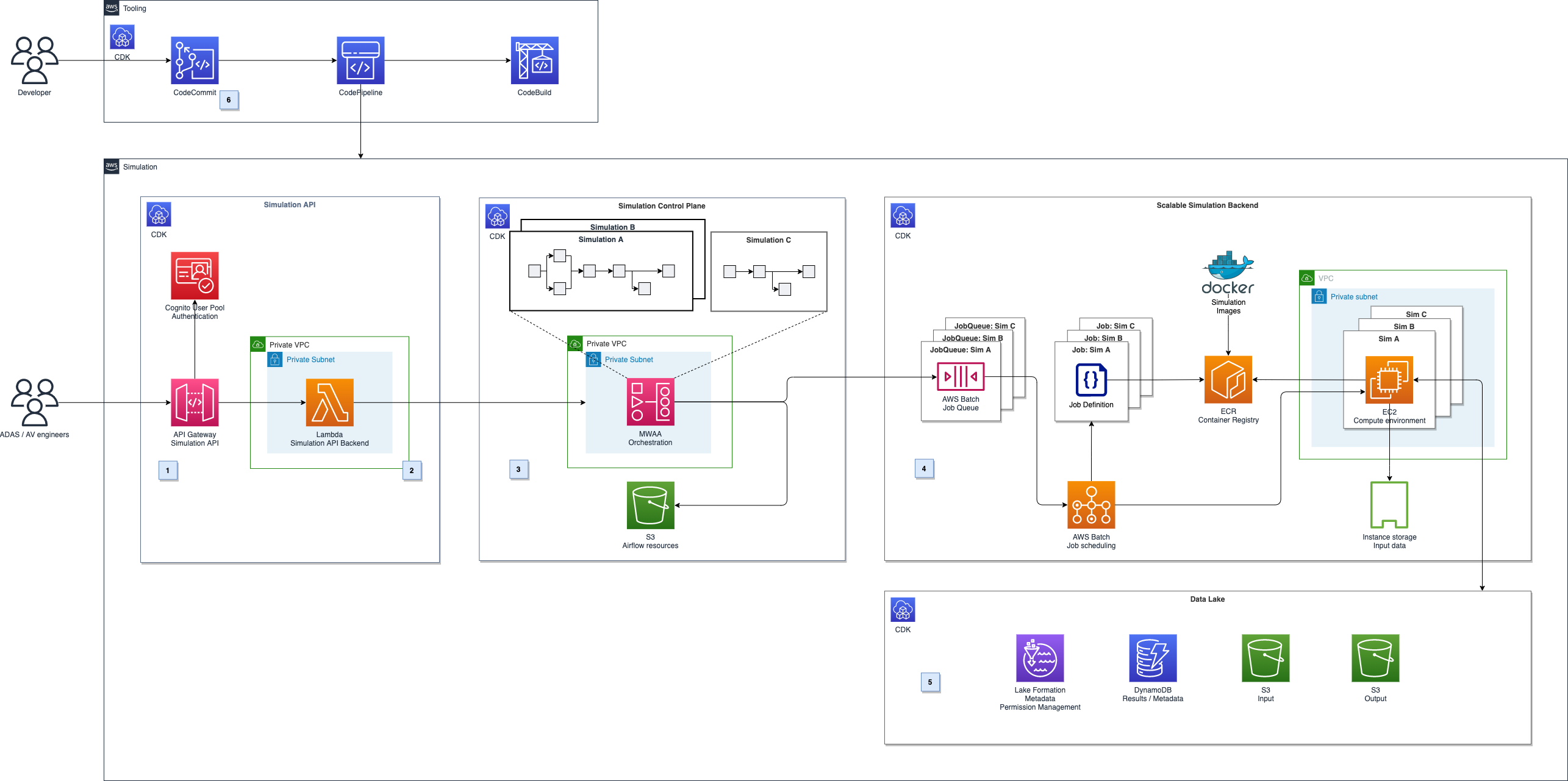
The following diagram shows a high-level overview of this solution.
Figure 1. Architecture diagram for autonomous driving simulation
It can be broken down into five major parts, illustrated in Figure 1.
Simulation API: Amazon API Gateway (label 1) provides a REST API for authenticated users to schedule or monitor simulation. It runs on Amazon Managed Workflows for Apache Airflow (MWAA) using AWS Lambda (label 2).
Simulation control plane: The simulation control plane (label 3) built on MWAA enables users to design and initiate workflows and integrate with AWS services.
Scalable compute backend: We leverage the parallelization and elastic scalability capabilities of AWS Batch to distribute the workload (label 4). Additionally, we want to be able to run proprietary software components as part of the simulation workflows and use highly customizable Amazon EC2 compute environments. For example, we can use GPU acceleration or Graviton-based instances for workloads that must run on ARM, instead of x86 architectures.
Autonomous Driving Data Lake (ADDL) integration: The simulations’ input and output data will be stored in a data lake (label 5) on Amazon S3. To provide efficient read and write access, data gets copied before each simulation run using RAID0 bundled ephemeral instance storage drives. After the simulation, results are written back to the data lake and are ready for reporting and analytics. We use AWS Lake Formation for metadata storage, data cataloging, and permission handling.
Automated deployment: The solution architecture’s deployment is fully automated using a CI/CD pipeline in AWS CodePipeline and AWS CodeBuild (label 6). We can then perform automated testing and deployment to multiple target environments.
In this blog we will focus on the simulation control plane, scalable compute backend, and ADDL integration.
Simulation control plane
In a typical simulation, there are tasks like data movement (copying input data and persisting the results). These steps can require high levels of parallelization or GPU support. In addition, they can involve third-party or proprietary software, specialized runtime environments, or architectures like ARM. To facilitate all task requirements, we will delegate task initiation to the AWS services that best match the requirements. Correct sequence of tasks is achieved by an orchestration layer. Decoupling the simulation orchestration from task initiation follows the key design pattern to separate concerns. This enables the architecture to be adapted to specific requirements.
For the high-level task orchestration, we’ll introduce a simulation control plane built on MWAA. Modeling all simulation tasks in a directed acyclic graph (DAG), MWAA performs scheduling and task initiation in the correct sequence. It also handles the integration with AWS’ services. You can intuitively monitor and debug the progress of a simulation run across different services and networks. For the workflow within CAEdge, we’ll use AWS Batch to run simulations that are packaged as Docker containers.
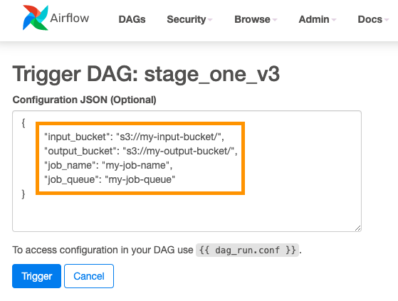
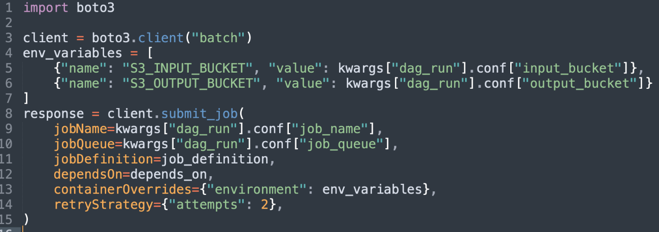
Parameterizable workflows: Airflow supports parameterization of DAGs by providing a JSON object when triggering a DAG run that can be accessed at runtime. This enables us to create a simulation execution framework in which we model the simulation steps. It lets you specify the simulations’ parameters such as which Docker container to execute, runtime configuration, or input and output data locations, see Figures 2 and 3.
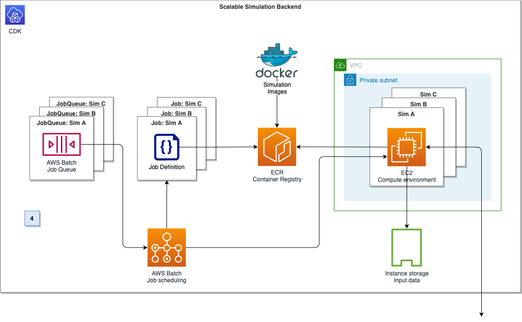
Choosing the compute option:Containers at AWS describes the services options for developers. Various factors can contribute to your decision-making. For the CAEdge platform, we want to run thousands of containers with fine-grained control over the underlying compute instance’s configuration. We also want to run containers in privileged mode, so AWS Batch on EC2 is a great match. Figure 4 outlines the compute backend’s architecture.
Figure 4. Compute backend architecture diagram
To run a Docker container on AWS Batch, we need three components: A job definition, a compute environment, and a job queue. The AWS Batch job definition specifies which job to run and how to run it. For example, we can define the Docker image to use, and specify the vCPU and memory configuration. The job definition will be submitted to a job queue, which in turn is linked to one or more compute environments. The compute environment specifies the compute configuration used to run a containerized workload, in addition to instance types and storage configurations. Creating a compute environment describes this more in detail. In the section ‘ADDL integration,’ we’ll describe how to select and configure the EC2 container instances to maximize network and disk I/O.
The AWS Batch array job feature can spin up thousands of independent, but similarly configured jobs. Instead of submitting a single job for each input file from the simulation control plane, we can instead submit a single array job. This provides the collection of input files as input. AWS Batch can spin up child jobs to process each entry of the collection in parallel, reducing operational overhead drastically.
With these components, we can now submit a job definition to a job queue from the simulation control plane, which will initiate on the corresponding compute environment.
ADDL integration
In the CAEdge platform, all simulation recordings and their metadata are stored and cataloged in the data lake. On average, single recordings are around 100 GB in size with simulation requests containing 100–300 recordings. A simulation request can therefore require 10–30 TB of data movement from S3 to the containers before the simulation starts. The containers’ performance will directly depend on I/O performance, as the input data is read and processed during execution. To provide the highest performance of data transfer and simulation workload, we need data storage options that maximize network and disk I/O throughput.
Choosing the storage option: For CAEdge’s simulation workloads, the storage solution acts as a temporary scratch space for the simulation containers’ input data. It should maximize I/O throughput. These requirements are met in the most cost-efficient way by choosing EC2 instances of the M5d family and their attached instance storage.
The M5d are general-purpose instances with NVMe-based SSDs, which are physically connected to the host server and provide block-level storage coupled to the lifetime of the instance. As described in the previous section, we configured AWS Batch to create compute environments using EC2’s M5d instances. While other storage options like Amazon Elastic File System (EFS) and Amazon Elastic Block Storage (EBS) can scale to match even demanding throughput scenarios, the simulation benefits from a high-performance, temporary storage location that is directly attached to the host.
Bundling the volumes: M5d instances can have multiple NVMe drives attached, depending on their size and storage configuration. To provide a single stable storage location for the simulation containers, bundle all attached NVMe SSDs into a single RAID0 volume during the instance’s launch, using a modified user data script. With this, we can provide a fixed storage location that can be accessed from the simulation containers. Additionally, we are distributing I/O operations evenly across all disks in the RAID0 configuration, which improves the read and write performance.
KPIs used for measurement
The SIL factor tells you how long the simulation takes compared to the duration of the recorded data.
SIL factor example:
For a recording with 60 minutes of data and a simulation duration of 120 minutes, the resulting SIL factor is 120 / 60 = 2. The simulation runs twice as long as real time.
For a recording with 60 minutes of data and a simulation duration of 60 minutes, the resulting SIL factor is 60 / 60 = 1. The simulation runs in real time.
Similarly, the aggregated SIL factor tells you how long the simulation for multiple recordings takes compared to the duration of the recorded data. It also factors in the horizontal scaling capabilities.
Aggregated SIL factor example:
For 3 recordings with 60 minutes of data and an overall simulation duration of 120 minutes, the resulting SIL factor is 120 / 3 * 60 = 0.67. The overall simulation is a third faster than real time.
Performance results
The storage optimizations described in the ADDL integration KPI section preceding, led to an improvement of the overall simulation duration of 50%. To benchmark the overall simulation platform’s performance, we created a simulation run with 15 recordings. The simulation run completed successfully with an aggregated SIL factor of 0.363, or, alternatively put, the simulation was roughly three times faster than real time. During production use, the platform will handle simulation runs with an average of 100-300 recordings. For these runs, the aggregated SIL factor is expected to be even smaller, as more simulations can be processed in parallel.
Conclusion
In this post, we showed how to design a platform for ADAS simulation workloads using the Bring Your Own Software-In-the-Loop (BYO-SIL) concept. We covered the key components including simulation control plane, scalable compute backend, and ADDL integration based on Continental Automotive Edge (CAEdge). We discussed the key performance benefits due to horizontal scalability and how to choose an optimized storage integration pattern. This led to an improvement of the overall simulation duration of 50%.
asset — any business logic code in a raw (e.g. SQL) or compiled (e.g. JAR) form to be executed as part of the user defined data pipeline.
data pipeline — a set of tasks (or jobs) to be executed in a predefined order (a.k.a. DAG) for the purpose of transforming data using some business logic.
Dataflow — Netflix homegrown CLI tool for data pipeline management.
job — a.k.a task, an atomic unit of data transformation logic, a non-separable execution block in the workflow chain.
namespace — unique label, usually representing a business subject area, assigned to a workflow asset to identify it across all other assets managed by Dataflow (e.g. security).
workflow — see “data pipeline”
Intro
The problem of managing scheduled workflows and their assets is as old as the use of cron daemon in early Unix operating systems. The design of a cron job is simple, you take some system command, you pick the schedule to run it on and you are done. Example:
0 0 * * MON /home/alice/backup.sh
In the above example the system would wake up every Monday morning and execute the backup.sh script. Simple right? But what if the script does not exist in the given path, or what if it existed initially but then Alice let Bob access her home directory and he accidentally deleted it? Or what if Alice wanted to add new backup functionality and she accidentally broke existing code while updating it?
The answers to these questions is something we would like to address in this article and propose a clean solution to this problem.
Let’s define some requirements that we are interested in delivering to the Netflix data engineers or anyone who would like to schedule a workflow with some external assets in it. By external assets we simply mean some executable carrying the actual business logic of the job. It could be a JAR compiled from Scala, a Python script or module, or a simple SQL file. The important thing is that this business logic can be built in a separate repository and maintained independently from the workflow definition. Keeping all that in mind we would like to achieve the following properties for the whole workflow deployment:
Versioning: we want both the workflow definition and its assets to be versioned and we want the versions to be tied together in a clear way.
Transparency: we want to know which version of an asset is running along with every workflow instance, so if there are any issues we can easily identify which version caused the problem and to which one we could revert, if necessary.
ACID deployment: for every scheduler workflow definition change, we would like to have all the workflow assets bundled in an atomic, durable, isolated and consistent manner. This way, if necessary, all we need to know is which version of the workflow to roll back to, and the rest would be taken care of for us.
While all the above goals are our North Star, we also don’t want to negatively affect fast deployment, high availability and arbitrary life span of any deployed asset.
Previous solutions
The basic approach to pulling down arbitrary workflow resources during workflow execution has been known to mankind since the invention of cron, and with the advent of “infinite” cloud storage systems like S3, this approach has served us for many years. Its apparent flexibility and convenience can often fool us into thinking that by simply replacing the asset in the S3 location we can, without any hassle, introduce changes to our business logic. This method often proves very troublesome especially if there is more than one engineer working on the same pipeline and they are not all aware of the other folks’ “deployment process”.
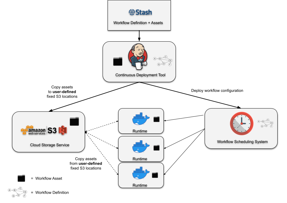
The slightly improved approach is shown on the diagram below.
In Figure 1, you can see an illustration of a typical deployment pipeline manually constructed by a user for an individual project. The continuous deployment tool submits a workflow definition with pointers to assets in fixed S3 locations. These assets are then separately deployed to these fixed locations. At runtime, the assets are retrieved from the defined locations in S3 and executed in the runtime container. Despite requiring users to construct the deployment pipeline manually, often by writing their own scripts from scratch, this design works and has been successfully used by many teams for years. That being said, it does have some drawbacks that are revealed as you try to add any amount of complexity to your deployment logic. Let’s discuss a few of them.
Does not consider branch/PR deployments
In any production pipeline, you want the flexibility of having a “safe” alternative deployment logic. For example, you may want to build your Scala code and deploy it to an alternative location in S3 while pushing a sandbox version of your workflow that points to this alternative location. Something this simple gets very complicated very quickly and requires the user to consider a number of things. Where should this alternative location be in S3? Is a single location enough? How do you set up your deployment logic to know when to deploy the workflow to a test or dev environment? Answers to these questions often end up being more custom logic inside of the user’s deployment scripts.
Cannot rollback to previous workflow versions
When you deploy a workflow, you really want it to encapsulate an atomic and idempotent unit of work. Part of the reason for that is the desire for the ability to rollback to a previous workflow version and knowing that it will always behave as it did in previous runs. There can be many reasons to rollback but the typical one is when you’ve recognized a regression in a recent deployment that was not caught during testing. In the current design, reverting to a previous workflow definition in your scheduling system is not enough! You have to rebuild your assets from source and move them to your fixed S3 location that your workflow points to. To enable atomic rollbacks, you can add more custom logic to your deployment scripts to always deploy your assets to a new location and generate new pointers for your workflows to use, but that comes with higher complexity that often just doesn’t feel worth it. More commonly, teams will opt to do more testing to try and catch regressions before deploying to production and will accept the extra burden of rebuilding all of their workflow dependencies in the event of a regression.
Runtime dependency on user-managed cloud storage locations
At runtime, the container must reach out to a user-defined storage location to retrieve the assets required. This causes the user-managed storage system to be a critical runtime dependency. If we zoom out to look at an entire workflow management system, the runtime dependencies can become unwieldy if it relies on various storage systems that are arbitrarily defined by the workflow developers!
Dataflow deployment with asset management
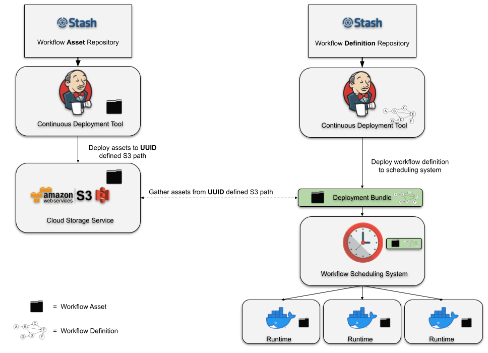
In the attempt to deliver a simple and robust solution to the managed workflow deployments we created a command line utility called Dataflow. It is a Python based CLI + library that can be installed anywhere inside the Netflix environment. This utility can build and configure workflow definitions and their assets during testing and deployment. See below diagram:
Figure 2. Dataflow asset management system.
In Figure 2, we show a variation of the typical manually constructed deployment pipeline. Every asset deployment is released to some newly calculated UUID. The workflow definition can then identify a specific asset by its UUID. Deploying the workflow to the scheduling system produces a “Deployment Bundle”. The bundle includes all of the assets that have been referenced by the workflow definition and the entire bundle is deployed to the scheduling system. At every scheduled runtime, the scheduling system can create an instance of your workflow without having to gather runtime dependencies from external systems.
The asset management system that we’ve created for Dataflow provides a strong abstraction over this deployment design. Deploying the asset, generating the UUID, and building the deployment bundle is all handled automatically by the Dataflow build logic. The user does not need to be aware of anything that’s happening on S3, nor that S3 is being used at all! Instead, the user is given a flexible UUID referencing system that’s layered on top of our scheduling system’s workflow DSL. Later in the article we’ll cover this referencing system in some detail. But first, let’s look at an example of deploying an asset and a workflow.
Deployment of an asset
Let’s walk through an example of a workflow asset build and deployment. Let’s assume we have a repository called stranger-data with the following structure:
Before deploying the assets, and especially if we made any changes to them, we can run unit tests to make sure that we didn’t break anything. In a typical Dataflow configuration this manual testing is optional because Dataflow continuous integration tests will do that for us on any pull-request.
Notice that the test command we use above not only executes unit test suites defined in our Scala and Python sub-projects, but it also renders and statically validates all the workflow definitions in our repo, but more on that later…
Assuming all tests passed, let’s now use the Dataflow command to build and deploy a new version of the Scala and Python assets into the Dataflow asset registry.
stranger-data$ dataflow project deploy
Building Python Assets: -> ./pyspark-workflow/hello_world/setup.py... CREATED ./pyspark-workflow/hello_world/dist/hello_world-0.0.1-py3.7.egg Summary: 1 successful, 0 failed.
The above list could come in handy, for example if we needed to find and access an older version of an asset deployed from a given branch and commit hash.
Deployment of a workflow
Now let’s have a look at the build and deployment of the workflow definition which references the above assets as part of its pipeline DAG.
Let’s list the workflow definitions in our repo again:
You can see from the above snippet that the write job wants to access some version of the JAR from the scala-workflow namespace. A typical workflow definition, written in YAML, does not need any compilation before it is shipped to the Scheduler API, but Dataflow designates a special step called “rendering” to substitute all of the Dataflow variables and build the final version.
The above expression ${dataflow.jar.scala-workflow} means that the workflow will be rendered and deployed with the latest version of the scala-workflow JAR available at the time of the workflow deployment. It is possible that the JAR is built as part of the same repository in which case the new build of the JAR and a new version of the workflow may be coming from the same deployment. But the JAR may be built as part of a completely different project and in that case the testing and deployment of the new workflow version can be completely decoupled.
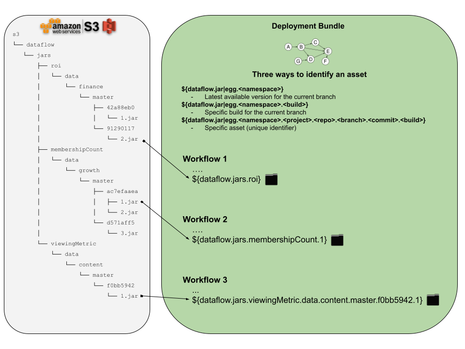
We showed above how one would request the latest asset version available during deployment, but with Dataflow asset management we can distinguish two more asset access patterns. An obvious next one is to specify it by all its attributes: asset type, asset namespace, git repo owner, git repo name, git branch name, commit hash and consecutive build number. There is one more extra method for a middle ground solution to pick a specific build for a given namespace and git branch, which can help during testing and development. All of this is part of the user-interface for determining how the deployment bundle will be created. See below diagram for a visual illustration.
Figure 3. A closer at the Deployment Bundle
In short, using the above variables gives the user full flexibility and allows them to pick any version of any asset in any workflow.
An example of the workflow deployment with the rendering step is shown below:
stranger-data$ dataflow project deploy
...
Building Scheduler Workflows:
 -> ./scala-workflow/main.sch.yaml... CREATED ./.workflows/scala-workflow.main.sch.rendered.yaml
 -> ./pyspark-workflow/main.sch.yaml... CREATED ./.workflows/pyspark-workflow.main.sch.rendered.yaml
Summary: 2 successful, 0 failed.
And here you can see what the workflow definition looks like before it is sent to the Scheduler API and registered as the latest version. Notice the value of the script variable of the write job. In the original code says ${dataflow.jar.scala-workflow} and in the rendered version it is translated to a specific file pointer:
The Infrastructure DSE team at Netflix is responsible for providing insights into data that can help the Netflix platform and service scale in a secure and effective way. Our team members partner with business units like Platform, OpenConnect, InfoSec and engage in enterprise level initiatives on a regular basis.
One side effect of such wide engagement is that over the years our repository evolved into a mono-repo with each module requiring a customized build, testing and deployment strategy packaged into a single Jenkins job. This setup required constant upkeep and also meant every time we had a build failure multiple people needed to spend a lot of time in communication to ensure they did not step on each other.
Last quarter we decided to split the mono-repo into separate modules and adopt Dataflow as our asset orchestration tool. Post deployment, the team relies on Dataflow for automated execution of unit tests, management and deployment of workflow related assets.
By the end of the migration process our Jenkins configuration went from:
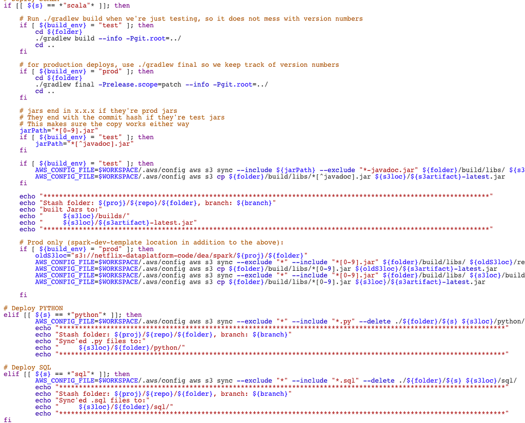
Figure 4. Real example of a deployment script.
to:
cd /dataflow_workspace
dataflow project deploy
The simplicity of deployment enabled the team to focus on the problems they set out to solve while the branch based customization gave us the flexibility to be our most effective at solving them.
Conclusions
This new method available for Netflix data engineers makes workflow management easier, more transparent and more reliable. And while it remains fairly easy and safe to build your business logic code (in Scala, Python, etc) in the same repository as the workflow definition that invokes it, the new Dataflow versioned asset registry makes it easier yet to build that code completely independently and then reference it safely inside data pipelines in any other Netflix repository, thus enabling easy code sharing and reuse.
One more aspect of data workflow development that gets enabled by this functionality is what we call branch-driven deployment. This approach enables multiple versions of your business logic and workflows to be running at the same time in the scheduler ecosystem, and makes it easy, not only for individual users to run isolated versions of the code during development, but also to define isolated staging environments through which the code can pass before it reaches the production stage. Obviously, in order for the workflows to be safely used in that configuration they must comply with a few simple rules with regards to the parametrization of their inputs and outputs, but let’s leave this subject for another blog post.
Credits
Special thanks to Peter Volpe, Harrington Joseph and Daniel Watson for the initial design review.
Though it seems like something out of a sci-fi movie, machine learning (ML) is part of our day-to-day lives. So often, in fact, that we may not always notice it. For example, social networks and mobile applications use ML to assess user patterns and interactions to deliver a more personalized experience.
However, AWS services provide many options for the integration of ML. In this post, we will show you some use cases that can enhance your platforms and integrate ML into your production systems.
Performing A/B testing on production traffic to compare a new ML model with the old model is a recommended step after offline evaluation.
This blog post explains how A/B testing works and how it can be combined with multi-armed bandit testing to gradually send traffic to the more effective variants during the experiment. It will teach you how to build it with AWS Cloud Development Kit (AWS CDK), architect your system for MLOps, and automate the deployment of the solutions for A/B testing.
This diagram shows the iterative process to analyze the performance of ML models in online and offline scenarios
Modularity is a key characteristic for modern applications. You can modularize code, infrastructure, and even architecture.
A modular architecture provides an architecture and framework that allows each development role to work on their own part of the system, and hide the complexity of integration, security, and environment configuration. This blog post provides an approach to building a modular ML workload that is easy to evolve and maintain across multiple teams.
A modular architecture allows you to easily assemble different parts of the system and replace them when needed
The accuracy of ML models can deteriorate over time because of model drift or concept drift. This is a common challenge when deploying your models to production. Have you ever experienced it? How would you architect a solution to address this challenge?
Without metrics and automated actions, maintaining ML models in production can be overwhelming. This blog post shows you how to design an MLOps pipeline for model monitoring to detect concept drift. You can then expand the solution to automatically launch a new training job after the drift was detected to learn from the new samples, update the model, and take into account the changes in the data distribution.
Concept drift happens when there is a shift in the distribution. In this case, the distribution of the newly collected data (in blue) starts differing from the baseline distribution (in green)
Moving from experimentation to production forces teams to move fast and automate their operations. Adopting scalable solutions for MLOps is a fundamental step to successfully create production-oriented ML processes.
This blog post provides an extended walkthrough of the ML lifecycle and explains how to optimize the process using Amazon SageMaker. Starting from data ingestion and exploration, you will see how to train your models and deploy them for inference. Then, you’ll make your operations consistent and scalable by architecting automated pipelines. This post offers a fraud detection use case so you can see how all of this can be used to put ML in production.
The ML lifecycle involves three macro steps: data preparation, train and tuning, and deployment with continuous monitoring
See you next time!
Thanks for reading! We’ll see you in a couple of weeks when we discuss how to secure your workloads in AWS.
Looking for more architecture content?AWS Architecture Center provides reference architecture diagrams, vetted architecture solutions, Well-Architected best practices, patterns, icons, and more!
Amazon processes hundreds of millions of financial transactions each day, including accounts receivable, accounts payable, royalties, amortizations, and remittances, from over a hundred different business entities. All of this data is sent to the eCommerce Financial Integration (eCFI) systems, where they are recorded in the subledger.
Ensuring complete financial reconciliation at this scale is critical to day-to-day accounting operations. With transaction volumes exhibiting double-digit percentage growth each year, we found that our legacy transactional-based financial reconciliation architecture proved too expensive to scale and lacked the right level of visibility for our operational needs.
In this post, we show you how we migrated to a batch processing system, built on AWS, that consumes time-bounded batches of events. This not only reduced costs by almost 90%, but also improved visibility into our end-to-end processing flow. The code used for this post is available on GitHub.
Legacy architecture
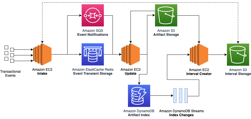
Our legacy architecture primarily utilized Amazon Elastic Compute Cloud (Amazon EC2) to group related financial events into stateful artifacts. However, a stateful artifact could refer to any persistent artifact, such as a database entry or an Amazon Simple Storage Service (Amazon S3) object.
We found this approach resulted in deficiencies in the following areas:
Cost – Individually storing hundreds of millions of financial events per day in Amazon S3 resulted in high I/O and Amazon EC2 compute resource costs.
Data completeness – Different events flowed through the system at different speeds. For instance, while a small stateful artifact for a single customer order could be recorded in a couple of seconds, the stateful artifact for a bulk shipment containing a million lines might require several hours to update fully. This made it difficult to know whether all the data had been processed for a given time range.
Complex retry mechanisms – Financial events were passed between legacy systems using individual network calls, wrapped in a backoff retry strategy. Still, network timeouts, throttling, or traffic spikes could result in some events erroring out. This required us to build a separate service to sideline, manage, and retry problematic events at a later date.
Scalability – Bottlenecks occurred when different events competed to update the same stateful artifact. This resulted in excessive retries or redundant updates, making it less cost-effective as the system grew.
Operational support – Using dedicated EC2 instances meant that we needed to take valuable development time to manage OS patching, handle host failures, and schedule deployments.
The following diagram illustrates our legacy architecture.
Evolution is key
Our new architecture needed to address the deficiencies while preserving the core goal of our service: update stateful artifacts based on incoming financial events. In our case, a stateful artifact refers to a group of related financial transactions used for reconciliation. We considered the following as part of the evolution of our stack:
Stateless and stateful separation
Minimized end-to-end latency
Scalability
Stateless and stateful separation
In our transactional system, each ingested event results in an update to a stateful artifact. This became a problem when thousands of events came in all at once for the same stateful artifact.
However, by ingesting batches of data, we had the opportunity to create separate stateless and stateful processing components. The stateless component performs an initial reduce operation on the input batch to group together related events. This meant that the rest of our system could operate on these smaller stateless artifacts and perform fewer write operations (fewer operations means lower costs).
The stateful component would then join these stateless artifacts with existing stateful artifacts to produce an updated stateful artifact.
As an example, imagine an online retailer suddenly received thousands of purchases for a popular item. Instead of updating an item database entry thousands of times, we can first produce a single stateless artifact that summaries the latest purchases. The item entry can now be updated one time with the stateless artifact, reducing the update bottleneck. The following diagram illustrates this process.
Minimized end-to-end latency
Unlike traditional extract, transform, and load (ETL) jobs, we didn’t want to perform daily or even hourly extracts. Our accountants need to be able to access the updated stateful artifacts within minutes of data arriving in our system. For instance, if they had manually sent a correction line, they wanted to be able to check within the same hour that their adjustment had the intended effect on the targeted stateful artifact instead of waiting until the next day. As such, we focused on parallelizing the incoming batches of data as much as possible by breaking down the individual tasks of the stateful component into subcomponents. Each subcomponent could run independently of each other, which allowed us to process multiple batches in an assembly line format.
Scalability
Both the stateless and stateful components needed to respond to shifting traffic patterns and possible input batch backlogs. We also wanted to incorporate serverless compute to better respond to scale while reducing the overhead of maintaining an instance fleet.
This meant we couldn’t simply have a one-to-one mapping between the input batch and stateless artifact. Instead, we built flexibility into our service so the stateless component could automatically detect a backlog of input batches and group multiple input batches together in one job. Similar backlog management logic was applied to the stateful component. The following diagram illustrates this process.
Current architecture
To meet our needs, we combined multiple AWS products:
AWS Step Functions – Orchestration of our stateless and stateful workflows
Amazon EMR – Apache Spark operations on our stateless and stateful artifacts
AWS Lambda – Stateful artifact indexing and orchestration backlog management
The following diagram illustrates our current architecture.
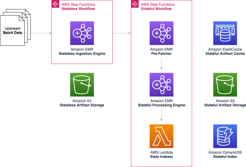
The following diagram shows our stateless and stateful workflow.
The AWS CloudFormation template to render this architecture and corresponding Java code is available in the following GitHub repo.
Stateless workflow
We used an Apache Spark application on a long-running Amazon EMR cluster to simultaneously ingest input batch data and perform reduce operations to produce the stateless artifacts and a corresponding index file for the stateful processing to use.
We chose Amazon EMR for its proven highly available data-processing capability in a production setting and also its ability to horizontally scale when we see increased traffic loads. Most importantly, Amazon EMR had lower cost and better operational support when compared to a self-managed cluster.
Stateful workflow
Each stateful workflow performs operations to create or update millions of stateful artifacts using the stateless artifacts. Similar to the stateless workflows, all stateful artifacts are stored in Amazon S3 across a handful of Apache Spark part-files. This alone resulted in a huge cost reduction, because we significantly reduced the number of Amazon S3 writes (while using the same amount of overall storage). For instance, storing 10 million individual artifacts using the transactional legacy architecture would cost $50 in PUT requests alone, whereas 10 Apache Spark part-files would cost only $0.00005 in PUT requests (based on $0.005 per 1,000 requests).
However, we still needed a way to retrieve individual stateful artifacts, because any stateful artifact could be updated at any point in the future. To do this, we turned to DynamoDB. DynamoDB is a fully managed and scalable key-value and document database. It’s ideal for our access pattern because we wanted to index the location of each stateful artifact in the stateful output file using its unique identifier as a primary key. We used DynamoDB to index the location of each stateful artifact within the stateful output file. For instance, if our artifact represented orders, we would use the order ID (which has high cardinality) as the partition key, and store the file location, byte offset, and byte length of each order as separate attributes. By passing the byte-range in Amazon S3 GET requests, we can now fetch individual stateful artifacts as if they were stored independently. We were less concerned about optimizing the number of Amazon S3 GET requests because the GET requests are over 10 times cheaper than PUT requests.
Overall, this stateful logic was split across three serial subcomponents, which meant that three separate stateful workflows could be operating at any given time.
Pre-fetcher
The following diagram illustrates our pre-fetcher subcomponent.
The pre-fetcher subcomponent uses the stateless index file to retrieve pre-existing stateful artifacts that should be updated. These might be previous shipments for the same customer order, or past inventory movements for the same warehouse. For this, we turn once again to Amazon EMR to perform this high-throughput fetch operation.
Each fetch required a DynamoDB lookup and an Amazon S3 GET partial byte-range request. Due to the large number of external calls, fetches were highly parallelized using a thread pool contained within an Apache Spark flatMap operation. Pre-fetched stateful artifacts were consolidated into an output file that was later used as input to the stateful processing engine.
Stateful processing engine
The following diagram illustrates the stateful processing engine.
The stateful processing engine subcomponent joins the pre-fetched stateful artifacts with the stateless artifacts to produce updated stateful artifacts after applying custom business logic. The updated stateful artifacts are written out across multiple Apache Spark part-files.
Because stateful artifacts could have been indexed at the same time that they were pre-fetched (also called in-flight updates), the stateful processor also joins recently processed Apache Spark part-files.
We again used Amazon EMR here to take advantage of the Apache Spark operations that are required to join the stateless and stateful artifacts.
State indexer
The following diagram illustrates the state indexer.
This Lambda-based subcomponent records the location of each stateful artifact within the stateful part-file in DynamoDB. The state indexer also caches the stateful artifacts in an Amazon ElastiCache for Redis cluster to provide a performance boost in the Amazon S3 GET requests performed by the pre-fetcher.
However, even with a thread pool, a single Lambda function isn’t powerful enough to index millions of stateful artifacts within the 15-minute time limit. Instead, we employ a cluster of Lambda functions. The state indexer begins with a single coordinator Lambda function, which determines the number of worker functions that are needed. For instance, if 100 part-files are generated by the stateful processing engine, then the coordinator might assign five part-files for each of the 20 Lambda worker functions to work on. This method is highly scalable because we can dynamically assign more or fewer Lambda workers as required.
Each Lambda worker then performs the ElastiCache and DynamoDB writes for all the stateful artifacts within each assigned part-file in a multi-threaded manner. The coordinator function monitors the health of each Lambda worker and restarts workers as needed.
Orchestration
We used Step Functions to coordinate each of the stateless and stateful workflows, as shown in the following diagram.
Every time a new workflow step ran, the step was recorded in a DynamoDB table via a Lambda function. This table not only maintained the order in which stateful batches should be run, but it also formed the basis of the backlog management system, which directed the stateless ingestion engine to group more or fewer input batches together depending on the backlog.
We chose Step Functions for its native integration with many AWS services (including triggering by an Amazon CloudWatchscheduled event rule and adding Amazon EMR steps) and its built-in support for backoff retries and complex state machine logic. For instance, we defined different backoff retry rates based on the type of error.
Conclusion
Our batch-based architecture helped us overcome the transactional processing limitations we originally set out to resolve:
Reduced cost – We have been able to scale to thousands of workflows and hundreds of million events per day using only three or four core nodes per EMR cluster. This reduced our Amazon EC2 usage by over 90% when compared with a similar transactional system. Additionally, writing out batches instead of individual transactions reduced the number of Amazon S3 PUT requests by over 99.8%.
Data completeness guarantees – Because each input batch is associated with a time interval, when a batch has finished processing, we know that all events in that time interval have been completed.
Simplified retry mechanisms – Batch processing means that failures occur at the batch level and can be retried directly through the workflow. Because there are far fewer batches than transactions, batch retries are much more manageable. For instance, in our service, a typical batch contains about two million entries. During a service outage, only a single batch needs to be retried, as opposed to two million individual entries in the legacy architecture.
High scalability – We’ve been impressed with how easy it is to scale our EMR clusters on the fly if we detect an increase in traffic. Using Amazon EMR instance fleets also helps us automatically choose the most cost-effective instances across different Availability Zones. We also like the performance achieved by our Lambda-based state indexer. This subcomponent not only dynamically scales with no human intervention, but has also been surprisingly cost-efficient. A large portion of our usage has fallen within the free tier.
Operational excellence – Replacing traditional hosts with serverless components such as Lambda allowed us to spend less time on compliance tickets and focus more on delivering features for our customers.
We are particularly excited about the investments we have made moving from a transactional-based system to a batch processing system, especially our shift from using Amazon EC2 to using serverless Lambda and big data Amazon EMR services. This experience demonstrates that even services originally built on AWS can still achieve cost reductions and improve performance by rethinking how AWS services are used.
Inspired by our progress, our team is moving to replace many other legacy services with serverless components. Likewise, we hope that other engineering teams can learn from our experience, continue to innovate, and do more with less.
Find the code used for this post in the following GitHub repository.
Special thanks to development team: Ryan Schwartz, Abhishek Sahay, Cecilia Cho, Godot Bian, Sam Lam, Jean-Christophe Libbrecht, and Nicholas Leong.
About the Authors
Tom Jin is a Senior Software Engineer for eCommerce Financial Integration (eCFI) at Amazon. His interests include building large-scale systems and applying machine learning to healthcare applications. He is based in Vancouver, Canada and is a fan of ocean conservation.
Karthik Odapally is a Senior Solutions Architect at AWS supporting our Gaming Customers. He loves presenting at external conferences like AWS Re:Invent, and helping customers learn about AWS. His passion outside of work is to bake cookies and bread for family and friends here in the PNW. In his spare time, he plays Legend of Zelda (Link’s Awakening) with his 4 yr old daughter.
The PinePhone is a Linux-based
smartphone made by PINE64 that runs free
and open-source software (FOSS); it is designed to
use a close-to-mainline Linux kernel. While many
smartphones already use the Linux kernel as part of Android, few run
distributions that are actually similar to those used on desktops and
laptops. The PinePhone is different, however; it provides an experience
that is much closer to normal desktop Linux, though it probably cannot
completely replace a full-featured smartphone—at least yet.
Version 2.38 of the GNU Binutils tool set has been released. Changes
include new hardware support (including for the LoongArch architecture),
various Unicode-handling improvements, a new --thin option to ar for the creation of thin archives, and more.
The collective thoughts of the interwebz
Manage Consent
To provide the best experiences, we use technologies like cookies to store and/or access device information. Consenting to these technologies will allow us to process data such as browsing behavior or unique IDs on this site. Not consenting or withdrawing consent, may adversely affect certain features and functions.
Functional
Always active
The technical storage or access is strictly necessary for the legitimate purpose of enabling the use of a specific service explicitly requested by the subscriber or user, or for the sole purpose of carrying out the transmission of a communication over an electronic communications network.
Preferences
The technical storage or access is necessary for the legitimate purpose of storing preferences that are not requested by the subscriber or user.
Statistics
The technical storage or access that is used exclusively for statistical purposes.The technical storage or access that is used exclusively for anonymous statistical purposes. Without a subpoena, voluntary compliance on the part of your Internet Service Provider, or additional records from a third party, information stored or retrieved for this purpose alone cannot usually be used to identify you.
Marketing
The technical storage or access is required to create user profiles to send advertising, or to track the user on a website or across several websites for similar marketing purposes.