Codacy Measures Developer Productivity using AWS Serverless

Post Syndicated from Catarina Gralha original https://aws.amazon.com/blogs/architecture/codacy-measures-developer-productivity-using-aws-serverless/

Codacy is a DevOps insights company based in Lisbon, Portugal. Since its launch in 2012, Codacy has helped software development and engineering teams reduce defects, keep technical debt in check, and ship better code, faster.

Codacy’s latest product, Pulse, is a service that helps understand and improve the performance of software engineering teams. This includes measuring metrics such as deployment frequency, lead time for changes, or mean time to recover. Codacy’s main platform is built on top of AWS products like Amazon Elastic Kubernetes Service (EKS), but they have taken Pulse one step further with AWS serverless.

In this post, we will explore the Pulse’s requirements, architecture, and the services it is built on, including AWS Lambda, Amazon API Gateway, and Amazon DynamoDB.

Pulse prototype requirements

Codacy had three clear requirements for their initial Pulse prototype.

  1. The solution must enable the development team to iterate quickly and have minimal time-to-market (TTM) to validate the idea.
  2. The solution must be easily scalable and match the demands of both startups and large enterprises alike. This was of special importance, as Codacy wanted to onboard Pulse with some of their existing customers. At the time, these customers already had massive amounts of information.
  3. The solution must be cost-effective, particularly during the early stages of the product development.

Enter AWS serverless

Codacy could have built Pulse on top of Amazon EC2 instances. However, this brings the undifferentiated heavy lifting of having to provision, secure, and maintain the instances themselves.

AWS serverless technologies are fully managed services that abstract the complexity of infrastructure maintenance away from developers and operators, so they can focus on building products.

Serverless applications also scale elastically and automatically behind the scenes, so customers don’t need to worry about capacity provisioning. Furthermore, these services are highly available by design and span multiple Availability Zones (AZs) within the Region in which they are deployed. This gives customers higher confidence that their systems will continue running even if one Availability Zone is impaired.

AWS serverless technologies are cost-effective too, as they are billed per unit of value, as opposed to billing per provisioned capacity. For example, billing is calculated by the amount of time a function takes to complete or the number of messages published to a queue, rather than how long an EC2 instance runs. Customers only pay when they are getting value out of the services, for example when serving an actual customer request.

Overview of Pulse’s solution architecture

An event is generated when a developer performs a specific action as part of their day-to-day tasks, such as committing code or merging a pull request. These events are the foundational data that Pulse uses to generate insights and are thus processed by multiple Pulse components called modules.

Let’s take a detailed look at a few of them.

Ingestion module

Figure 1. Pulse ingestion module architecture

Figure 1. Pulse ingestion module architecture

Figure 1 shows the ingestion module, which is the entry point of events into the Pulse platform and is built on AWS serverless applications as follows:

  • The ingestion API is exposed to customers using Amazon API Gateway. This defines REST, HTTP, and WebSocket APIs with sophisticated functionality such as request validation, rate limiting, and more.
  • The actual business logic of the API is implemented as AWS Lambda functions. Lambda can run custom code in a fully managed way. You only pay for the time that the function takes to run, in 1-millisecond increments. Lambda natively supports multiple languages, but customers can also bring their own runtimes or container images as needed.
  • API requests are authorized with keys, which are stored in Amazon DynamoDB, a key-value NoSQL database that delivers single-digit millisecond latency at any scale. API Gateway invokes a Lambda function that validates the key against those stored in DynamoDB (this is called a Lambda authorizer.)
  • While API Gateway provides a default domain name for each API, Codacy customizes it with Amazon Route 53, a service that registers domain names and configures DNS records. Route 53 offers a service level agreement (SLA) of 100% availability.
  • Events are stored in raw format in Pulse’s data lake, which is built on top of AWS’ object storage service, Amazon Simple Storage Service (S3). With Amazon S3, you can store massive amounts of information at low cost using simple HTTP requests. The data is highly available and durable.
  • Whenever a new event is ingested by the API, a message is published in Pulse’s message bus. (More information later in this post.)

Events module

Figure 2. Pulse events module architecture

Figure 2. Pulse events module architecture

The events module handles the aggregation and storage of events for actual consumption by customers, see Figure 2:

  • Events are consumed from the message bus and processed with a Lambda function, which stores them in Amazon Redshift.
  • Amazon Redshift is AWS’ managed data warehouse, and enables Pulse’s users to get insights and metrics by running analytical (OLAP) queries with the highest performance.
  • These metrics are exposed to customers via another API (the public API), which is also built on API Gateway.
  • The business logic for this API is implemented using Lambda functions, like the Ingestion module.

Message bus

Figure 3. Message bus architecture

Figure 3. Message bus architecture

We mentioned earlier that Pulse’s modules communicate messages with each other via the “message bus.” When something occurs at a specific component, a message (event) is published to the bus. At the same time, developers create subscriptions for each module that should receive these messages. This is known as the publisher/subscriber pattern (pub/sub for short), and is a fundamental piece of event-driven architectures.

With the message bus, you can decouple all modules from each other. In this way, a publisher does not need to worry about how many or who their subscribers are, or what to do if a new one arrives. This is all handled by the message bus.

Pulse’s message bus is built like this, shown in Figure 3:

  • Events are published via Amazon Simple Notification Service (SNS), using a construct called a topic. Topics are the basic unit of message publication and consumption. Components are subscribed to this topic, and you can filter out unwanted messages.
  • Developers configure Amazon SNS subscriptions to have the events sent to a queue, which provides a buffering layer from which workers can process messages. At the same time, queues also ensure that messages are not lost if there is an error. In Pulse’s case, these queues are implemented with Amazon Simple Queue Service (SQS).

Other modules

There are other parts of Pulse architecture that also use AWS serverless. For example, user authentication and sign-up are handled by Amazon Cognito, and Pulse’s frontend application is hosted on Amazon S3. This app is served to customers worldwide with low latency using Amazon CloudFront, a content delivery network.

Summary and next steps

By using AWS serverless, Codacy has been able to reduce the time required to bring Pulse to market by staying focused on developing business logic, rather than managing servers. Furthermore, Codacy is confident they can handle Pulse’s growth, as this serverless architecture will scale automatically according to demand.

How to deploy AWS Network Firewall to help protect your network from malware

Post Syndicated from Ajit Puthiyavettle original https://aws.amazon.com/blogs/security/how-to-deploy-aws-network-firewall-to-help-protect-your-network-from-malware/

Protecting your network and computers from security events requires multi-level strategies, and you can use network level traffic filtration as one level of defense. Users need access to the internet for business reasons, but they can inadvertently download malware, which can impact network and data security. This post describes how to use custom Suricata Rules with AWS Network Firewall to add protections that prevent users from downloading malware. You can use your own internal list, or a list from commercial or open-source threat intelligence feeds.

Network Firewall is a managed service that makes it easy to deploy essential network protection for all of your Amazon Virtual Private Cloud (Amazon VPC) Infrastructure. Network Firewall’s flexible rules engine lets you define firewall rules, giving you fine-grained control over network traffic, such as blocking outbound requests to prevent the spread of potential malware.

Features of Network Firewall

This section describes features of Network Firewall that help improve the overall security of your network.

Network Firewall:

  • Is a managed Amazon Web Services (AWS) service, so you don’t have to build and maintain the infrastructure to host the network firewall.
  • Integrates with AWS Firewall Manager, which allows you to centrally manage security policies and automatically enforce mandatory security policies across existing and newly created accounts and virtual private clouds (VPCs).
  • Protects application availability by filtering inbound internet traffic using tools such as access control list (ACL) rules, stateful inspection, protocol detection, and intrusion prevention.
  • Provides URL, IP address, and domain-based outbound traffic filtering to help you meet compliance requirements, stop potential data leaks, and block communication with known malware hosts.
  • Gives you control and visibility of VPC-to-VPC traffic to logically separate networks that host sensitive applications or line-of-business resources.
  • Complements existing network and application security services on AWS by providing control and visibility to layer 3 through 7 network traffic for your entire VPC.

Automating deployment of Network Firewall and management of Network Firewall rules support management at-scale and help in timely response, as Network Firewall is designed to block access to insecure sites before they impact your resources. For the solution in this blog post, you’ll use an AWS CloudFormation template to deploy the network architecture with Network Firewall.

Solution architecture

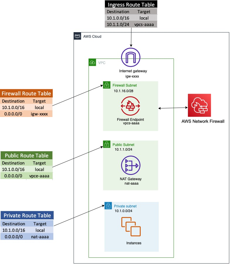
Figure 1 shows a sample architecture to demonstrate how users are able to download malware files, and how you can prevent this using network firewall rules.

Network Firewall is deployed in a single VPC architecture, where it is placed in line with the traffic to and from the internet.

Figure 1. Network architecture diagram

Figure 1. Network architecture diagram

The network architecture shown in Figure 1 includes three subnets:

  1. A network firewall subnet
    Hosts the Network Firewall endpoint interface. All outbound traffic from this network goes through the internet gateway.
  2. A public subnet
    Hosts a NAT gateway. The next hop from the public subnet is the Network Firewall endpoint, where all traffic can be inspected before being forwarded to the internet.
  3. A private network subnet
    Used to host the client instances. All outbound traffic from this network goes to the NAT gateway endpoint.

In the network architecture shown in Figure 1, only one AZ is shown for simplicity, but best practices recommend deploying infrastructure across multiple AZs

To run the CloudFormation deployment template

  1. To set up the architecture shown in Figure 1, launch the provided CloudFormation deployment template using the Launch stack button in step 2 below.
    This CloudFormation template:

    • Sets up VPCs and appropriate subnets as required by the network architecture.
    • Creates a route table with appropriate routes and attaches it to the appropriate subnet (i.e. private subnet, firewall subnet, public subnet).
    • Creates a test instance with appropriate security groups.
    • Deploys Network Firewall with firewall policy.
    • Creates a Rule Group SampleStatefulRulegroupName with Suricata rules, which is not attached to a firewall policy
  2. To launch the stack, click the Launch Stack button below.
  3. Select the Launch Stack button to launch the template

  4. Name the newly created stack (for example, nfw-stack).
  5. The template will also install two sample rules that will be used to protect against accessing two sample malware site URLs, but it will not automatically attach them to a firewall policy
  6. You can see that Network Firewall with firewall policy was deployed as part of the basic CloudFormation deployment. It also created Suricata rules in rule groups, but is not yet attached to the firewall policy.

    Note: Unless you attach the rule to the Network Firewall, it will not provide the required protection.

Example: confirming vulnerability

We have identified two sample URLs that contain malware to use for demonstration.

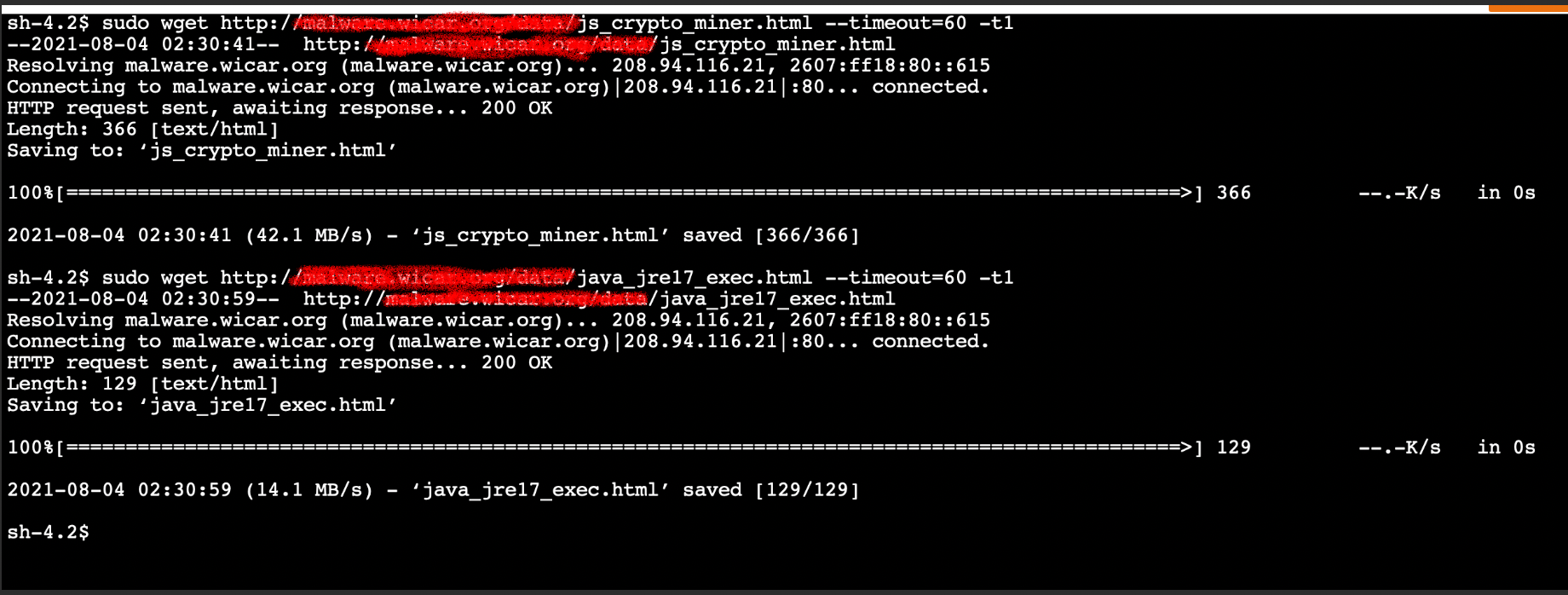
In the example screen shot below, we tested vulnerability by logging into test instance using AWS Session Manager. and at the shell prompt, used wget to access and download a malware file.

Figure 2 that follows is a screenshot of how a user could access and download two different malware files.

Note: Since these URLs contain malware files, we do not recommend users perform this test, but are providing a screenshot as a demonstration. If you wish to actually test ability to download files, use URLs you know are safe for testing.

Figure 2. Insecure URL access

Figure 2. Insecure URL access

Network Firewall policies

Before the template creates the Network Firewall rule group, it creates a Network Firewall policy and attaches it to the Network Firewall. An AWS Network Firewall firewall policy defines the monitoring and protection behavior for a firewall. The details of the behavior are defined in the rule groups that you add to your policy.

Network Firewall rules

A Network Firewall rule group is a reusable set of criteria for inspecting and handling network traffic. You can add one or more rule groups to a firewall policy as part of policy configuration. The included template does this for you.

Network Firewall rule groups are either stateless or stateful. Stateless rule groups evaluate packets in isolation, while stateful rule groups evaluate them in the context of their traffic flow. Network Firewall uses a Suricata rules engine to process all stateful rules.

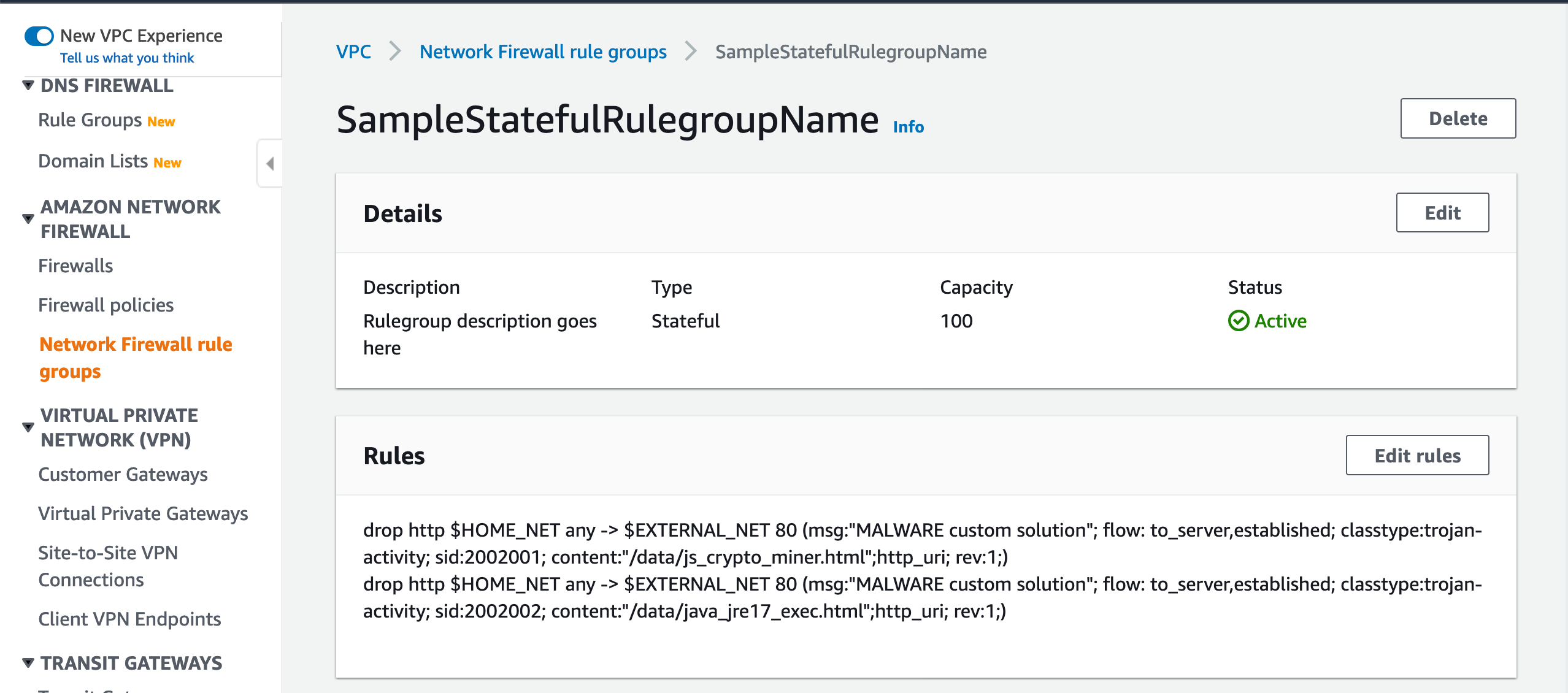
Suricata rules can be used to create a Network Firewall stateful rule to prevent insecure URL access. Figure 3 shows the Suricata rules that the template adds and attaches to the Network Firewall policy in order to block access to the sample malware URLs used in the previous example.

Figure 3. Suricata rules in a Network Firewall rule group

Figure 3. Suricata rules in a Network Firewall rule group

Attach the rule group to the Network Firewall policy

When you launched the CloudFormation template, it automatically created these rules in the rule group. You will now be attaching this rule group to the firewall policy in order to enable the protection. You will need similar rules to block the test URLs that are used for your testing.

Figure 3 shows two Suricata rules that have been configured to block the insecure malware URLs.

To add Suricata rules to Network Firewall

To improve site security and protect against downloading malware, you can add Suricata rules to Network Firewall to secure your site. You’ll do this by:

  1. Creating and attaching a firewall policy to the Network Firewall.
  2. Creating rules as part of rule groups, which are attached to the firewall policy
  3. Testing to verify that access to malware URLs from the instance is blocked.

Let’s review Suricata Rules that are created, which can be attached to Network Firewall.

Suricata rule parts

Each Suricata rule has three parts:

  1. Action
  2. drop action that should be taken

  3. Header
  4. http this is the traffic protocol

    $HOME_NET anywhere $HOME_NET is a Suricata variable. By default it is set to the CIDR range of the VPC where Network Firewall is deployed and any refers to any source port

    $EXTERNAL_NET 80 where $EXTERNAL_NET 80 is a Suricata standard variable that refers to traffic destination, and 80 refers to the destination port

    -> is the direction that tells in which direction the signature has to match

  5. Options
  6. msg “MALWARE custom solution” – gives textual information about the signature and the possible alert

    flow to_server,established – it is used to match on the direction of the flow and established refers to match on established connections

    classtype trojan-activity – gives information about the classification of rules and alerts

    sid:xxxxx gives every signature its own id

    content “xxxx” – This keyword is very important and it identifies the pattern that your signature should match.

    http_uri is a content modifier that helps you match specifically and only on the request URI

    rev:xxx this goes along with sid keyword. It represents the version of the signature

The signatures in the Suricate rule shown in Figure 3 will block traffic that matches the http_uri contents /data/js_crypto_miner.html and /data/java_jre17_exec.html when the traffic is initiated from the VPC to the public network.

To attach a rule group to an existing Network Firewall

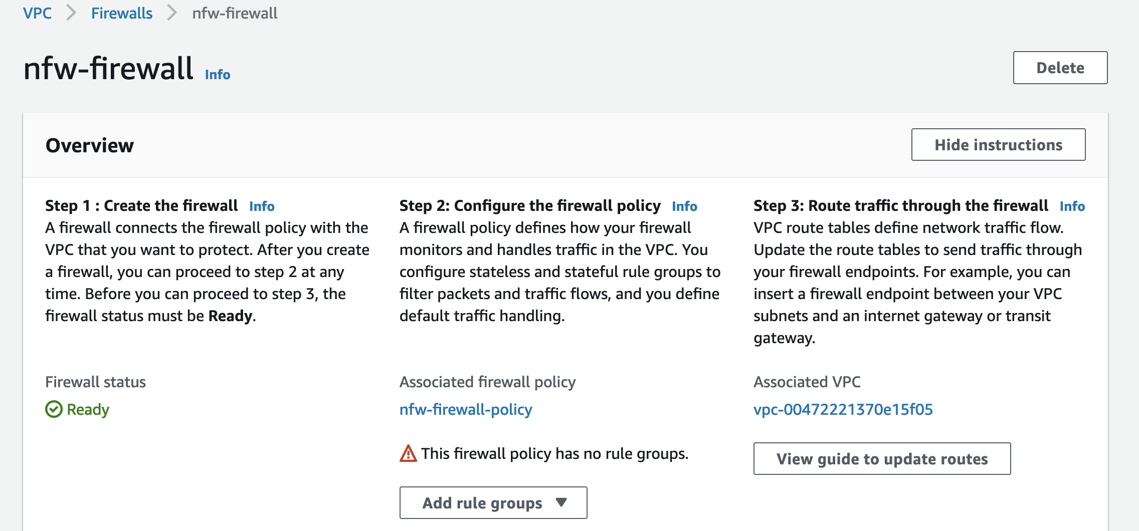
In Figure 4, the Network Firewall has a policy attached. but it does not have a rule group

Figure 4. A policy is attached, but not a rule group

Figure 4. A policy is attached, but not a rule group

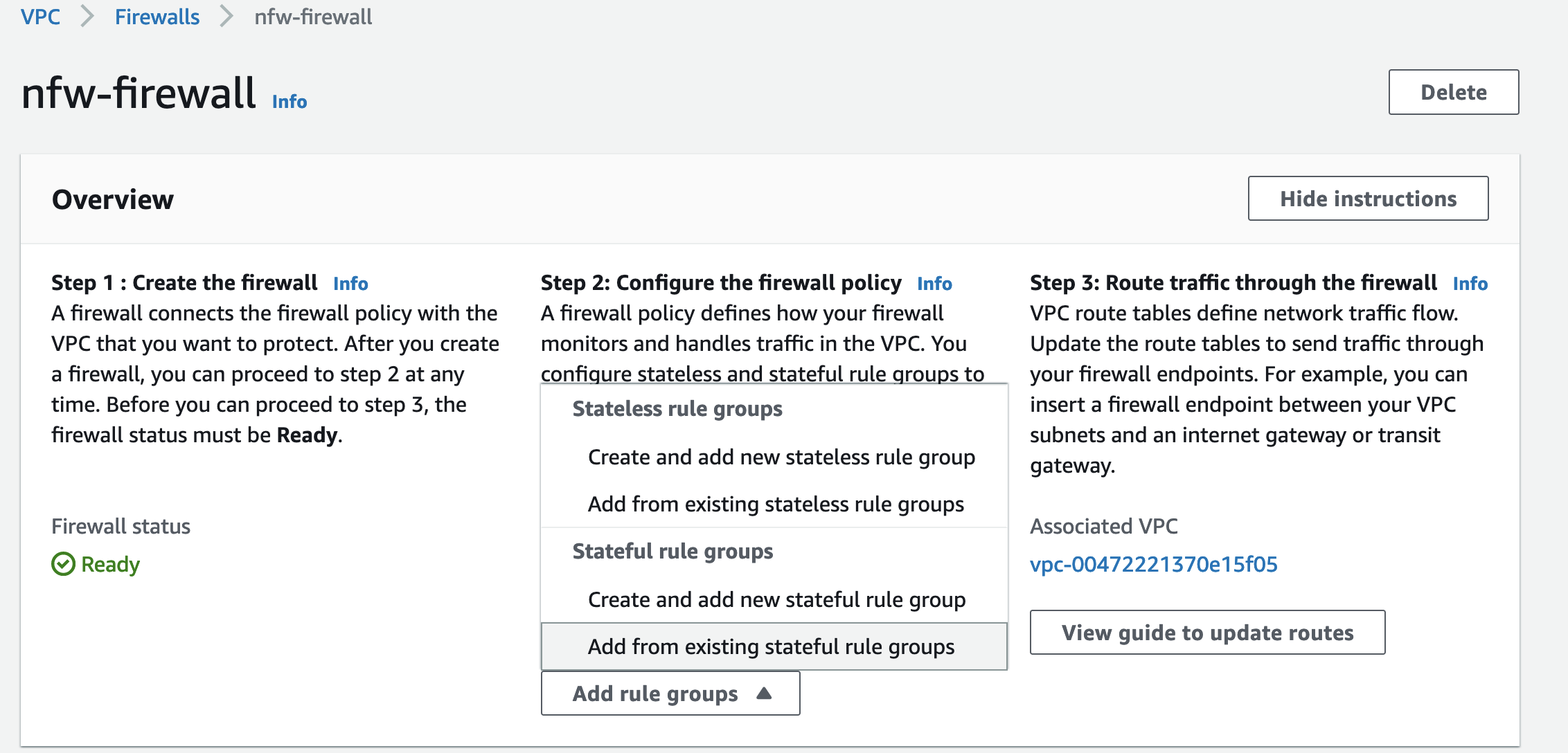
  1. As shown in Figure 5, choose Add rule group to start adding your Suricata rule to the Network Firewall.
  2. Choose Add from existing stateful rule groups to attach an already created Suricata rule group.
  3. Figure 5. Choose Add rule group

    Figure 5. Choose Add rule group

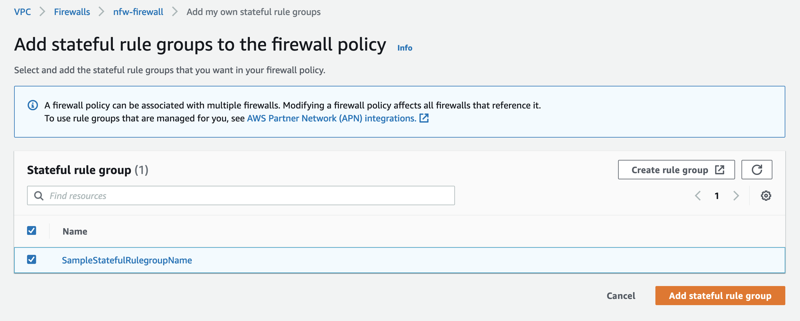
  4. Figure 6 shows the Suriacata rule groups that are already created. SampleStatefulRulegroupName is the rule group created by the CloudFormation template.
  5. Select the rule group and choose Add stateful rule group to finish adding the rule group to Network Firewall.
  6. Figure 6. Review the rule groups that are already created

    Figure 6. Review the rule groups that are already created

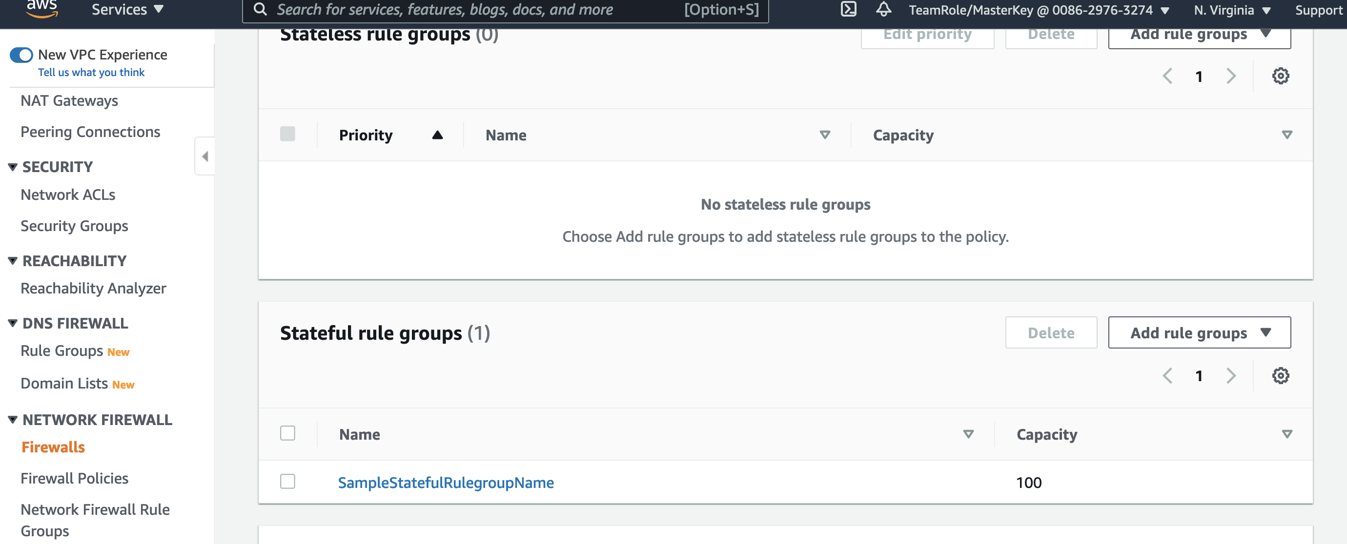
  7. Figure 7 shows that the rule group SampleStatefulRulegroupName is now part of the Stateful rule group section of Network Firewall screen, which completes adding Suricata rules to Network Firewall.
  8. Figure 7. Shows the new rule group is now added

    Figure 7. Shows the new rule group is now added

Example: validating the solution

Your Network Firewall is now configured to block malware URLs that are defined in the rulegroup SampleStatefulRulegroupName.

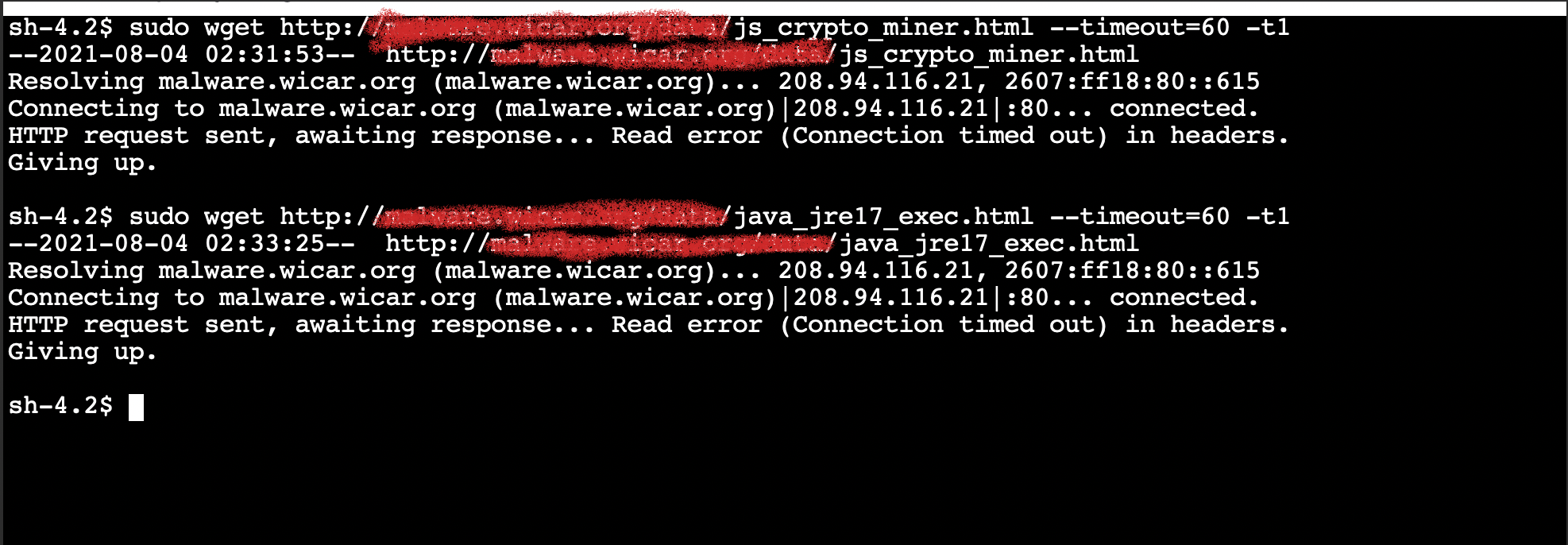
As in the example above where we confirmed vulnerability, Figure 8 shows how to validate that the solution is now protecting your users from accessing malware sites.

Figure 8 shows a user trying to access the same insecure URLs we tested earlier and shows that the URLs are now blocked and the attempted connection times out.

Note: Since these URLs contain malware files, we do not recommend users perform this test, but are providing a screenshot as a demonstration. If you wish to actually test ability to download files, use URLs you know are safe for testing.

Figure 8. Insecure URL access blocked

Figure 8. Insecure URL access blocked

Validating blocking access helps your security team ensure that users or applications on your network cannot download malware. You can add similar rules for any URLs you identify as insecure. SOC operators are typically not familiar with updating CloudFormation templates, but you can use a deployment pipeline where the data required for the rule is stored in Amazon DynamoDB and use AWS Lambda functions to automate updating rules.

Now that you have an example running, you should implement a complete rule set that meets your requirement from a publicly available malware list such as CISSECURITY MALWARE LIST.

Cleanup

AWS resources created for testing can result in additional costs. Since this environment used a CloudFormation template, you can remove all AWS resources associated with the solution by deleting the CloudFormation stack you named previously (for example, nfw-stack).

Conclusion

This blog describes an approach for preventing users from downloading malware. The solution presented uses AWS Network Firewall to secure your environment by blocking access to the specified malware URLs. The supplied CloudFormation template can be used to automate this protection, and to easily set up a test environment to simulate the scenario.

For additional best practice information, see:

If you have feedback about this post, submit comments in the Comments section below. If you have questions about this post, contact AWS Support.

.

Want more AWS Security news? Follow us on Twitter.

Author

Ajit Puthiyavettle

Ajit is a Solution Architect working with enterprise clients, architecting solutions to achieve business outcomes. He is passionate about solving customer challenges with innovative solutions. His experience is with leading DevOps and security teams for enterprise and SaaS (Software as a Service) companies.

Add comparative and cumulative date/time calculations in Amazon QuickSight

Post Syndicated from Emily Zhu original https://aws.amazon.com/blogs/big-data/add-comparative-and-cumulative-date-time-calculations-in-amazon-quicksight/

Amazon QuickSight recently added native support for comparative (e.g., year-over-year) and cumulative (e.g., year-to-date) period functions which allow you to easily introduce these calculations in business reporting, trend analysis and time series analysis. This allows authors in QuickSight to implement advanced calculations without having to use complicated date offsets in calculations to achieve such datetime-aware comparisons.

In this post, we introduce the new period functions and their capabilities, and demonstrate several typical use cases. We also discuss several scenarios to extend the usage of the period functions, which will be useful in more advanced situations.

New period functions

Before we demonstrate use cases, let’s go over the new period function suite and see what new functions we now support. We can divide period functions into two main groups: comparative (period over period) functions and cumulative (period to date) functions.

Comparative (period over period) functions

You can use period over period functions to compare measures at different time periods, such as year, quarter, and month. For example, you can compute a year-over-year increase in sales, or week-over-week percentage revenue changes.

A typical comparative period function has the syntax periodOverPeriodDifference(measure, date, period, offset), with two optional arguments: period and offset.

You can use the period argument in the function to define the period granularity of the calculation. The granularity of YEAR means year-over-year computation, Quarter means quarter-over-quarter, and so on. If the period argument is left empty, the calculation changes based on the period granularity that is chosen (in the field well) to be displayed in the visual.

You can also use the offset argument to specify how many periods apart you want to compute the comparison. For instance, a period of a quarter with an offset of 2 means comparing against the previous two quarters.

Note that period and offset have to be both specified or both left empty. You can’t specify just one of them.

The following table summarizes the three available period over period functions.

Function Name Function Type Description
periodOverPeriodDifference Table Calculation Calculates the difference of a measure over two different time periods as specified by period granularity and offset.
periodOverPeriodLastValue Table Calculation Calculates the last (previous) value of a measure from a previous time period as specified by period granularity and offset.
periodOverPeriodPercentDifference Table Calculation Calculates the percent difference of a measure over two different time periods as specified by period granularity and offset.

Cumulative (period to date) functions

You can use period to date functions to calculate metrics within a given period-to-date window. There are two main types of cumulative functions.

  • “OverTime” functions, which are table calculations and return outputs for each row in the visual.

E.g., you can use periodToDateCountOverTime with WEEK granularity to compute a series of week-to-date new customer counts to track the fluctuation of customer engagement.

  • Aggregation functions, which output an aggregated value for a fixed period-to-date time range.

E.g., periodtoDateSum with YEAR granularity returns a single value for the total of the metric from the beginning of the year to the endDate provided in the formula. If left blank, the default endDate takes now(), which is the moment when users load the dashboard.

The following table summarizes the period to date functions.

Function Name Function Type Description
periodToDateAvgOverTime Table Calculation Calculates the average of a measure for a given time granularity (for instance, a quarter) up to a point in time.
periodToDateCountOverTime Table Calculation Calculates the count of a dimension or measure for a given time granularity (for instance, a quarter) up to a point in time.
periodToDateMaxOverTime Table Calculation Calculates the maximum of a measure or date for a given time granularity (for instance, a quarter) up to a point in time.
periodToDateMinOverTime Table Calculation Calculates the minimum of a measure or date for a given time granularity (for instance, a quarter) up to a point in time.
periodToDateSumOverTime Table Calculation Calculates the sum of a measure for a given time granularity (for instance, a quarter) up to a point in time.
periodToDateAvg Aggregation Averages the set of numbers in the specified measure for a given time granularity (for instance, a quarter) up to a point in time.
periodToDateCount Aggregation Calculates the number of values in a dimension or measure for a given time granularity (for instance, a quarter) up to a point in time, including duplicates.
periodToDateMax Aggregation Returns the maximum value of the specified measure for a given time granularity (for instance, a quarter) up to a point in time.
periodToDateMedian Aggregation Returns the median value of the specified measure for a given time granularity (for instance, a quarter) up to a point in time.
periodToDateMin Aggregation Returns the minimum value of the specified measure or date for a given time granularity (for instance, a quarter) up to a point in time.
periodToDatePercentile Aggregation Calculates the percentile based on the actual numbers in the measure for a given time granularity (for instance, a quarter) up to a point in time.
periodToDatePercentileCont Aggregation Calculates the percentile based on a continuous distribution of the numbers in the measure for a given time granularity (for instance, a quarter) up to a point in time.
periodToDateStDev Aggregation Calculates the standard deviation of the set of numbers in the specified measure for a given time granularity (for instance, a quarter) up to a point in time based on a sample.
periodToDateStDevP Aggregation Calculates the population standard deviation of the set of numbers in the specified measure for a given time granularity (for instance, a quarter) up to a point in time based on a sample.
periodtoDateSum Aggregation Adds the set of numbers in the specified measure for a given time granularity (for instance, a quarter) up to a point in time.
periodToDateVar Aggregation Calculates the sample variance of the set of numbers in the specified measure for a given time granularity (for instance, a quarter) up to a point in time.
periodToDateVarP Aggregation Calculates the population variance of the set of numbers in the specified measure for a given time granularity (for instance, a quarter) up to a point in time.

Use case 1: Using a period over period function to analyze sales growth in fixed and dynamic granularity

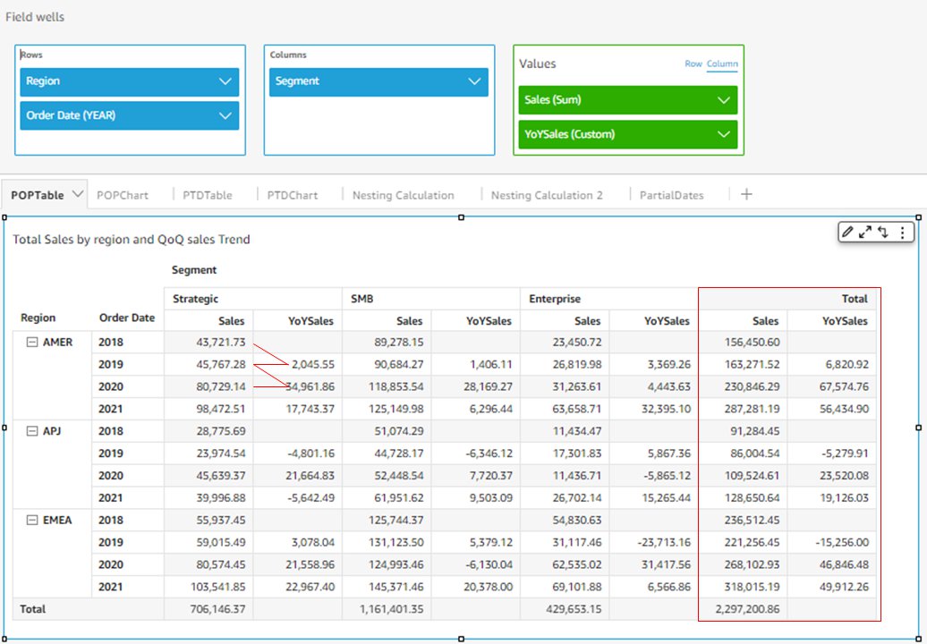
Let’s dive into how period over period functions can support typical business and financial use cases. The following example uses periodOverPeriodDifference to calculate YoY sales growth. Because we have Segment and Region in the visual, the YoY sales is calculated for each segment and region.

We define the measure of YoYSales with the following formula: YoYSales=periodOverPeriodDifference(sum(Sales),{Order Date},YEAR,1)

The first argument, sum(Sales), tells the function to calculate based on this measure. The second argument, Order Date, specifies the date/time column from which Year information is extracted. The third argument, YEAR, fixes the granularity of this calculation. When this optional argument is specified, this measure always returns YoY (not QoQ or MoM) no matter how Order Date is selected (in the field well) to be displayed in the visual. The fourth argument, 1, specifies the offset of the comparison. In this example, it means we want to compare the sales of each order date with the same date of the previous year. The measure returns empty for order dates of 2018, because no previous periods exist to be compared with.

The period functions are working with totals and subtotals. By adding the total for columns into the visual, you can see the total sales and total YoYSales for each region.

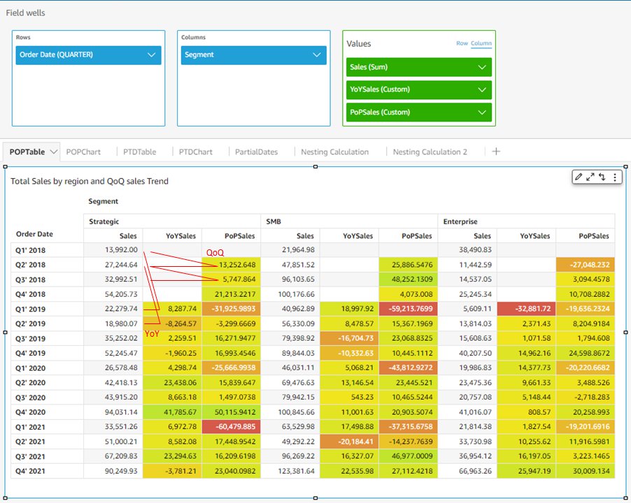
If you leave the optional argument of period granularity empty, meaning change the formula to PoPSales=periodOverPeriodDifference(sum(Sales),{Order Date})as shown in the following example, the time period of the calculation is then determined by the granularity of Order Date displayed on the visual. In the following example, Order Date is chosen to display at quarter level (in the field well), so PoPSales dynamically calculates the QoQ sales growth. Changing Order Date to the monthly level updates the measure to calculate MoM. For PoPSales, only Q1 2018 returns empty because that’s the only quarter that doesn’t have a previous quarter to compare with.

If we add YoYSales from the previous example to this visual, it calculates YoY sales growth at the quarter level (compares sales of Q1 2019 with Q1 2018). This demonstrates the difference between a fixed granularity and a dynamic granularity of period over period functions.

The period over period functions can differentiate between a positive change (increase) and negative change (decrease). Therefore, when we add the conditional formatting to the visual, it’s very straightforward to see the financial performance of each period (green is good, red is bad).

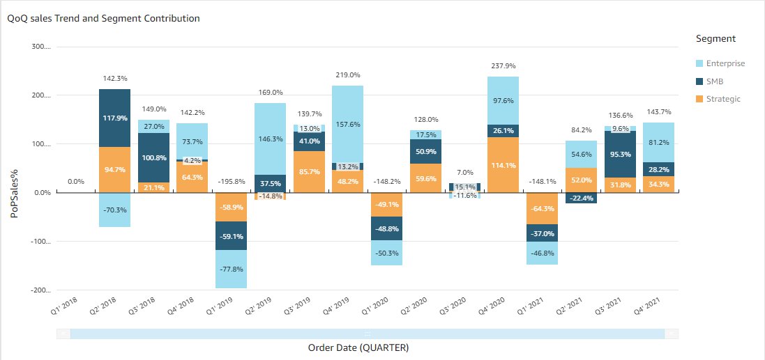
Similarly, you can use periodOverPeriodPercentDifference to calculate relative sales growth over time. You can add dimensions into the visual to dive further into business insights, such as analyzing the breakdown of each business segment’s sales change by quarter, and their contribution to the total sales increase. We use the formula PoPSales%=periodOverPeriodPercentDifference(sum(Sales),{Order Date}).

Use case 2: Using a period to date function to track YTD sales in table calculations and aggregations

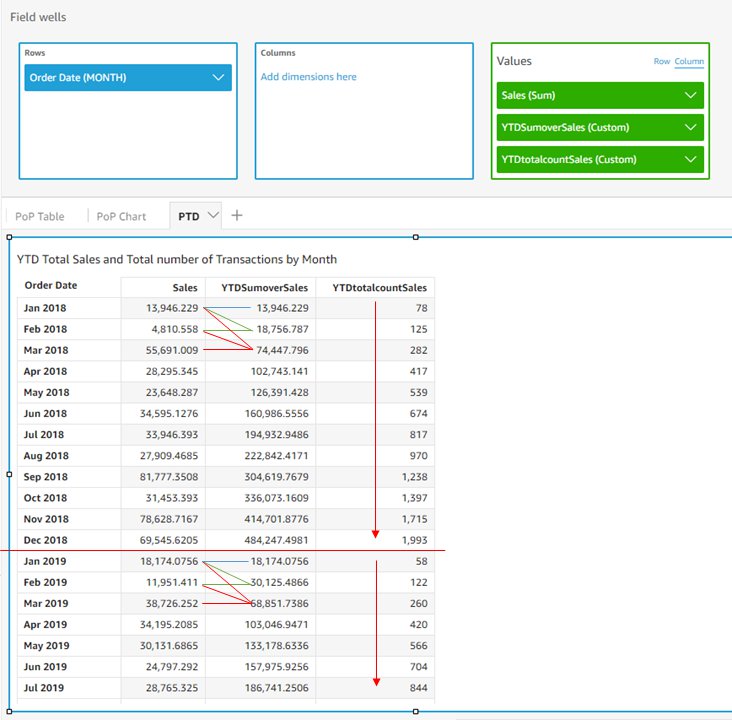
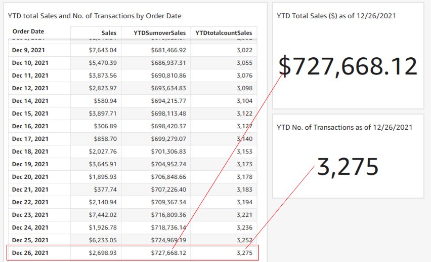
Similar to period over period functions, the period to date function suite provides a quick and easy way to calculate year-to-date (YTD) or quarter-to-date (QTD) metrics. In the following example, we use the formula of YTDSumoverSales=periodToDateSumOverTime(sum(Sales),{Order Date},YEAR), and YTDtotalcountSales=periodToDateSumOverTime(count(Sales),{Order Date},YEAR) to calculate YTD sales and YTD total number of transactions.

Contrary to period over period functions, the third argument of period to date functions, period, isn’t optional. Therefore, the calculation granularity is always fixed. In this example, with the granularity defined as YEAR, this measure always calculates YTD, instead of QTD or MTD. Because Order Date is displayed at the monthly level, this calculation outputs the YTD sales of each month, and starts over again in January for the next year. As shown in the result table, YTDSumoverSales of January 2018 is the monthly sales of January 2018, and YTDSumoverSales of February 2018 is the monthly sales of January 2018 plus that of February 2018. And YTDSumoverSales of January 2019 goes back to the monthly sales of January 2019.

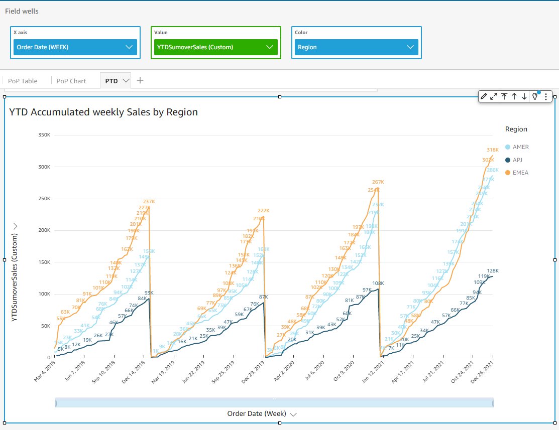
You can further dive into the details by populating the calculations in a line chart, and adding more dimensions into the analysis. The following example shows the YTD weekly sales growth trend for each region along the past four years, and uncovers some interesting sales competition between AMER and EMEA in year 2021.

In addition to the table calculations, the aggregation period functions are particularly useful when you need to build KPI charts to evaluate YTD metrics in a real-time manner. In the following example, we use the aggregation period to date functions to build two KPI charts to track the YTD total sales, and YTD total number of transactions. For the date December 26, 2021, the timestamp results match the corresponding table calculations for the date of December 26, 2021 in the table. The following table summarizes the formulas.

Formula Formula Type
YTDSumoverSales=periodToDateSumOverTime(sum(Sales),{Order Date},YEAR) Table Calculation
YTDtotalcountSales=periodToDateSumOverTime(count(Sales),{Order Date},YEAR) Table Calculation
YTDSumSales=periodToDateSum(Sales,{Order Date},YEAR) Aggregation (KPI chart)
YTDCountSales=periodToDateCount(Sales,{Order Date},YEAR) Aggregation (KPI chart)

Advanced use case 1: Date/time awareness with period functions

Period functions are not only easier to define and read, they’re also date/time-aware, meaning the functions are calculated based on a date/time-based offset instead of a fixed number of rows. It can solve two major problems that were not possible to be addressed before.

Period functions can handle varying period duration

If you want to calculate the daily MoM sales increase, you can’t use a fixed offset on each month because the number of days of each month are different (31 days for January and 28 or 29 days for February).

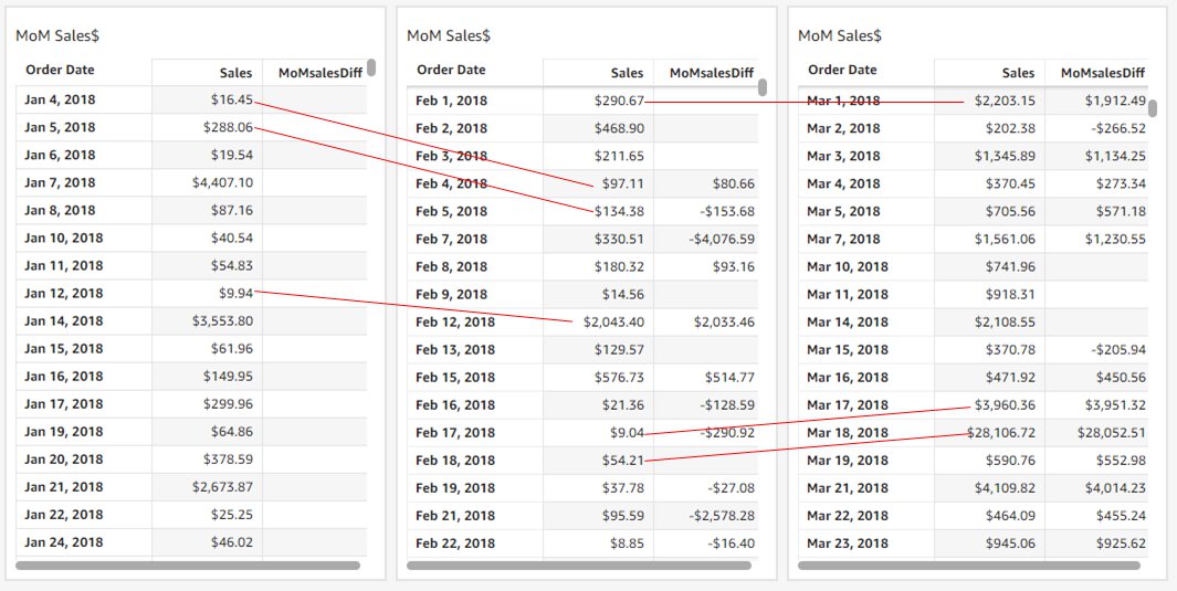
Period functions are calculated based on calendar dates instead of a fixed offset. In the following example, we use the formula MoMsalesDiff=periodOverPeriodDifference(sum(Sales),{Order Date},MONTH,1). The daily MoM increase is calculated correctly based on the day of the month. The sales of the first day of the month are compared with the first day of the previous month, and the same applies to all other days. (Visuals are duplicated for demonstration purposes.)

Period functions can handle sparse (missing) data points

Not all datasets can guarantee a complete set of dates. In the previous example, sales data of January 1, 2018, is missing. Using the workaround based on a fixed offset can cause a problem here because we compare February 1, 2018, with a different date instead of January 1, 2018. Period functions always compare measures by date/time offsets so that only desired dates are compared. In the previous example, MoMsalesDiff shows empty for February 1, 2018, because of the missing data of January 1, 2018.

Advanced use case 2: Nesting period functions with other calculations

Now that we can use period over period and period to date functions to create calculated fields, we can nest these functions with other calculations to drive more advanced analysis.

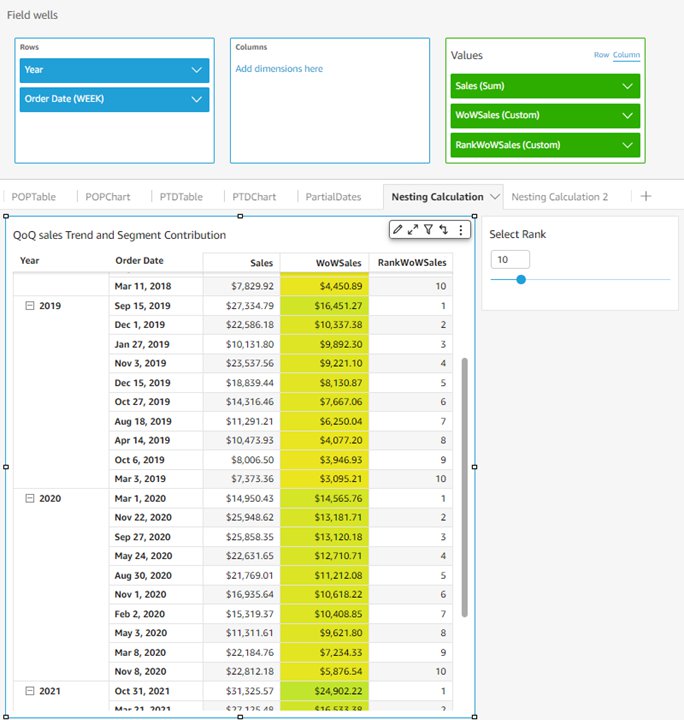
For example, you may want to know for each year, what are the top 10 weeks of the year in regards to week-over-week sales growth. You can do this by calculating WoWSales first: WoWSales=periodOverPeriodDifference(sum(Sales), {Order Date}, WEEK, 1). Then you nest it with the denseRank window function: RankWoWSales=denseRank([WoWSales DESC],[{YEAR}]). This wouldn’t be possible using the fixed-row based workaround, which is implemented using on-visual calculations instead of calculated fields. In the following visual, the top 10 weeks of each year with the highest sales growth are fetched by a simple filter on RankWoWSales.

You can even nest the period functions with other period functions to generate interesting insights. For example, you can calculate a monthly YoY growth based on the monthly YTD number of transactions. The following formula demonstrates the capability of nesting a YTD calculated field inside a YoY calculated field:

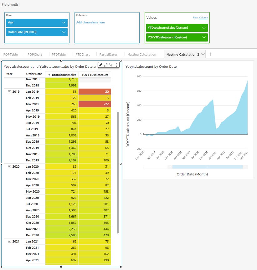
YTDtotalsountSales=periodToDateSumOverTime(count(Sales),{Order Date},YEAR)
YoYYTDSalesCount=periodOverPeriodDifference(YTDtotalcountSales,{Order Date},YEAR,1)

The results in the following visual show a YoY growth based on a YTD accumulated number of transactions instead of the absolute monthly numbers.

Advanced use case 3: Partial period comparisons

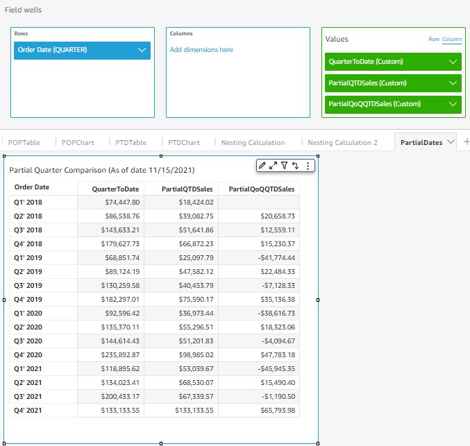
Finally, we discuss a third advanced use case: partial period comparison. Imagine it’s November 15, 2021 (which is the 46th day of the last quarter of 2021), and you want to calculate 4 to compare the performance of this quarter with past quarters, but only using the first 46 days of each quarter instead of the whole quarter. This requires a calculated field using periodOverPeriodDifference nested with the sumIf() window function.

The following example demonstrates using a nested calculated field to address this use case:

QuarterToDate=periodToDateSumOverTime(sum(Sales), {Order Date}, QUARTER)
PartialQTDSales=sumIf(Sales, dateDiff(truncDate("Q", {Order Date}), {Order Date}, "HH") <= dateDiff(truncDate("Q", now()), now(), "HH"))
PartialQoQQTDSales=periodOverPeriodDifference(sumif(Sales, {Order Date} <= addDateTime(dateDiff(truncDate("Q", now()), now(), "HH"), "HH", truncDate("Q", {Order Date}))), {Order Date}, QUARTER, 1)

PartialQTDSales computes how many hours from the beginning of this quarter to the current date and uses sumIf() to calculate the total sales of that period of each quarter. partialQoQQTDSales then nests the periodOverPeriodDifference function with PartialQTDSales to find the partial QoQ differences. Such a comparison based on a partial period isn’t feasible without the new date/time-aware period functions.

Conclusion

In this blog, we introduced new QuickSight period functions which enable quick and powerful date/time-based calculations. We reviewed comparative and cumulative period functions (i.e., period over period and period to date), discussed two major use cases (fixed vs. dynamic granularity and table calculation vs. aggregation), and extended the usage to three advanced use cases. Period functions are now generally available in all supported QuickSight Regions.

Looking forward to your feedback and stories on how you apply these calculations for your business needs.


About the Authors

Emily Zhu is a Senior Product Manager at Amazon QuickSight, AWS’s cloud-native, fully managed SaaS BI service. She leads the development of QuickSight core analytics and calculations capability. Before joining AWS, she was working in the Amazon Prime Air drone delivery program and the Boeing company as senior strategist for several years. Emily is passionate about potentials of cloud-based BI solutions and looks forward to helping customers to advance in their data-driven strategy making.

Rajkumar Haridoss is a Senior Software Development Engineer for AWS QuickSight. He is the lead engineer on the Query Generation team and works on back-end calculations, query planning, and query generation layer in QuickSight. Outside of work, he likes spending quality time with family and 4-year-old.

Protecting Holocaust educational websites

Post Syndicated from Omer Yoachimik original https://blog.cloudflare.com/protecting-holocaust-educational-websites/

Protecting Holocaust educational websites

Protecting Holocaust educational websites

Today is the International Holocaust Remembrance Day. On this day, we commemorate the victims that were murdered by the Nazis and their accomplices.

During the Holocaust, and in the events that led to it, the Nazis exterminated one third of the European Jewish population. Six million Jews, along with countless other members of minority and disability groups, were murdered because the Nazis believed they were inferior.

Cloudflare’s Project Galileo provides free protection to at-risk groups across the world including Holocaust educational and remembrance websites. During the past year alone, Cloudflare mitigated over a quarter of a million cyber threats launched against Holocaust-related websites.

Antisemitism and the Final Solution

In the Second World War and the years leading up to it, antisemitism served as the foundation of racist laws and fueled violent Pogroms against Jews. The tipping point was a night of violence known as the Kristallnacht (“Night of Broken Glass”). Jews and other minority groups were outlawed, dehumanized, persecuted and killed. Jewish businesses were boycotted, Jewish books burned and synagogues destroyed. Jews, Roma and other “enemies of the Reich” were forced into closed ghettos and concentration camps. Finally, as part of the Final Solution for the Jewish Question, Germany outlined a policy to deliberately and systematically exterminate the Jewish race in what came to be known as the Holocaust.

As part of the Final Solution, the Nazis deployed mobile killing units. Jews were taken to forests near their villages, forced to dig mass graves, undress, and then shot — falling into the mass graves they dug. This was the first step. However, this was “inefficient”. More “efficient” solutions were engineered using deadly gas. Eventually, six main extermination camps were established. They were extremely “efficient” at exterminating humans. Initially, the Nazis experimented with gas vans for mass extermination. Later, they built and operated gas chambers which could kill more humans and do it faster. After being gassed, prisoners would load the bodies into ovens in crematoriums to be burned. In one of the larger death camps, Auschwitz-Birkenau, more than one million Jews were murdered — some 865,000 were gassed and burned on arrival.

Fighting racism with education

Seventy-seven years later, sadly, racism and antisemitism are once again on the rise and have gained traction across Europe during the pandemic and across UK university campuses. Earlier this week, United Nations Secretary-General António Guterres decried the resurgence of antisemitism and said that “…the rise in antisemitism — the oldest form of hate and prejudice — has seen new reports of physical attacks, verbal abuse, the desecration of Jewish cemeteries, synagogues vandalized, and last week the hostage-taking of the rabbi and members of Beth Israel Congregation in Colleyville, Texas.”

It is through education that we will defeat bigotry and racism, and we will do our part at Cloudflare — through education and by supporting Holocaust educational organizations.

“Our response to ignorance must be education”
– United Nations Secretary-General António Guterres

Supporting Holocaust educational organizations with Project Galileo

As part of Project Galileo, we currently provide free security and performance products to more than 1,500 organizations in 111 countries. These organizations are targeted by cyber attacks due to their critical work. These groups include human rights defenders, independent media and journalists, and organizations that work in strengthening democracy. Among them are organizations dedicated to educating about the horrors of the Holocaust, and preserving and telling the stories of the victims and survivors of the Holocaust to younger and future generations.

Protecting Holocaust educational websites

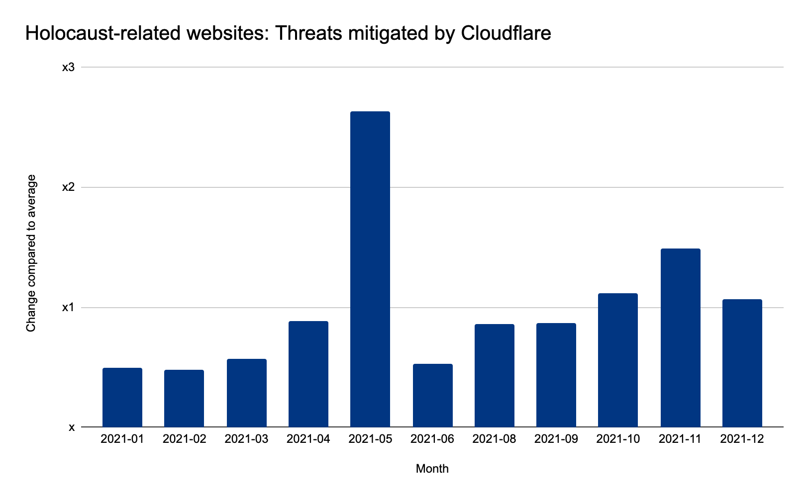
Over the past year, we’ve seen cyber attacks on Holocaust-related websites gradually increase throughout the year. These attacks include mostly application-layer attacks that were automatically detected and mitigated by Cloudflare’s Web Application Firewall and DDoS Protection systems.

In May 2021, cyber attacks on Holocaust-related websites peaked as they increased by 263% compared to their monthly average.

Protecting Holocaust educational websites

Applying to Project Galileo

Cloudflare’s mission is to help build a better Internet. Part of this mission includes protecting free expression online for vulnerable groups.

The Internet can be a powerful tool in this matter. However, organizations often face attacks from powerful and entrenched opponents, yet operate on limited budgets and lack the resources to secure themselves against malicious traffic intended to silence them. If they are silenced, the Internet stops fulfilling its promise.

To combat the threats, Cloudflare’s Project Galileo provides robust security and performance products for at-risk public interest websites at no cost. Application to Project Galileo is open to any vulnerable public interest website. You can apply via our partners or apply directly to Project Galileo if you don’t have any affiliation with our trusted partners.

A note from Cloudflare’s Jewish employees

Many of us, like myself, are descendants of Holocaust survivors. My grandparents fled from Nazi-occupied Poland to survive. Sadly, my grandparents — as other elderly survivors, are no longer with us. Many of us have faced antisemitism in various forms. Together, we are part of Cloudflare’s Employee Resource Group for Cloudflare’s Jewish community: Judeoflare. We have a responsibility to make sure the world remembers and never forgets the atrocities of the Holocaust and what racism and antisemitism can lead to.

Protecting Holocaust educational websites

Making the web better. With blocks!

Post Syndicated from Joel Spolsky original https://www.joelonsoftware.com/2022/01/27/making-the-web-better-with-blocks/

You’ve probably seen web editors based on the idea of blocks. I’m typing this in WordPress, which has a little + button that brings up a long list of potential blocks that you can insert into this page:

This kind of “insert block” user interface concept is showing up in almost every blogging tool, web editor, note-taking app, and content management system. People like it and it makes sense.

We have seem to have standardized on one thing: the / key to insert a new block. Everything else, though, is completely proprietary and non-standard.

I thought, wouldn’t it be cool if blocks were interchangeable and reusable across the web?

Until now, every app that wants blocks has to implement them from scratch. Want a calendar block? Some kind of fancy Kanban board? Something to embed image galleries? Code it up yourself, buddy.

As a result of the non-standardization of blocks, our end-users suffer. If someone is using my blog engine, they can only use those blocks that I had time to implement. Those blocks may be pretty basic or incomplete. Users might want to use a fancier block that they saw in WordPress or Medium or Notion, but my editor doesn’t have it. Blocks can’t be shared or moved around very easily, and our users are limited to the features and capabilities that we had time to re-implement.

To fix this, we’re going to create a protocol called the Block Protocol.

It’s open, free, non-proprietary, we want it to be everywhere on the web.

It’s just a protocol that embedding applications can use to embed blocks. Any block can be used in any embedding application if they all follow the protocol.

Our hope is that this will make life much easier for app developers to support a huge variety of block types. At the same time, anyone can develop a block once and have it work in any blog platform, note-taking app, or content management system. It is all 100% free, open, and any sample code we develop showing how to use the protocol will be open-source.

We’ve released a very early draft of the Block Protocol, and we’ve started building some very simple blocks and a simple editor that can host them.

We’re hoping to foster an open source community that creates a huge open source library of amazing blocks:

What can be a block?

  • Anything that makes sense in a document: a paragraph, list, table, diagram, or a kanban board.
  • Anything that makes sense on the web: an order form, a calendar, a video.
  • Anything that lets you interact with structured or typed data: I’ll get to that in a minute.

If you work on any kind of editor—be it a blogging tool, a note-taking app, a content management system, or anything like that—you should allow your users to embed blocks that conform to the Block Protocol. This way you can write the embedding code once and immediately make your editor able to embed a rich variety of block types with no extra work on your part.

If you work on any kind of custom data type that might make sense to embed in web pages, you should support the Block Protocol. That way anybody with a hosting application that supports the protocol can embed your custom data type.

Because it’s all 100% open, we hope that the Block Protocol will become a web standard and commonly used across the Internet.

That will mean that common block types, from paragraphs and lists to images and videos, will get better and better. But it will also mean that some esoteric block types will be embeddable anywhere. Want to create a block that shows the Great Circle routing for a flight between two airports? Write the code for the block once and it can be embedded anywhere.

Oh, and one more thing. Blocks can be highly structured, that is, they can have types. That means that they magically become machine-readable without screen scraping. For example, if you want to create an event block to represent an event on a calendar, you will be able to specify a schema that describes the event data type in a standard way. That way tools like calendars can instantly parse and understand web pages that contain your event block, reliably.

Over time, it will mean that anyone can easy publish complex, typed data sets on the web that are automatically machine-readable without extra work. (Have you ever seen one of those websites where there’s a link to “download the data set in .XLS format”? Yeah, say goodbye to that.)

We’re going public with this very early in the development process because we need a lot of help!

Everything we have so far is version 0.1. It’s simple and not very good yet and going to need some iteration before it has the hope of truly being a useful web protocol.

This is an open protocol, free and non-proprietary, and it’s going to make the open web much better if widely adopted, so we need to start getting people involved early, giving us feedback, and building new things!

Go read more about the Block Protocol now!

[$] An attic for LibreOffice Online

Post Syndicated from original https://lwn.net/Articles/882460/rss

In mid-December, Thorsten Behrens, a board member for the Document Foundation (TDF),
posted a
seemingly simple proposal
for an “attic” that would become the home of
abandoned projects. No specific projects were named as the first intended
residents of the attic, but the proposal
clearly related to the LibreOffice
Online
(LOOL) project. The following
discussion made it clear that the unhappiness around LOOL has yet to fade
away, and that the Foundation still has some work to do when it comes to
defining its relationship with its corporate members.

Migrating to Cloudflare Email Routing

Post Syndicated from Celso Martinho original https://blog.cloudflare.com/migrating-to-cloudflare-email-routing/

Migrating to Cloudflare Email Routing

A few days ago Google announced that the users from the “G Suite legacy free edition” would need to switch to the paid edition before May 1, 2022, to maintain their services and accounts working. Because of this, many people are now considering alternatives.

One use case for G Suite legacy was handling email for custom domains.

In September, during Birthday Week, we announced Cloudflare Email Routing. This service allows you to create any number of custom email addresses you want on top of the domains you already have with Cloudflare and automatically forward the incoming traffic to any destination inboxes you wish.

Email Routing was designed to be privacy-first, secure, powerful, and very simple to use. Also, importantly, it’s available to all our customers for free.

The closed beta allowed us to keep improving the service and make it even more robust, compliant with all the technical nuances of email, and scalable. Today we’re pleased to report that we have over two hundred thousand zones testing Email Routing in production, and we started the countdown to open beta and global availability.

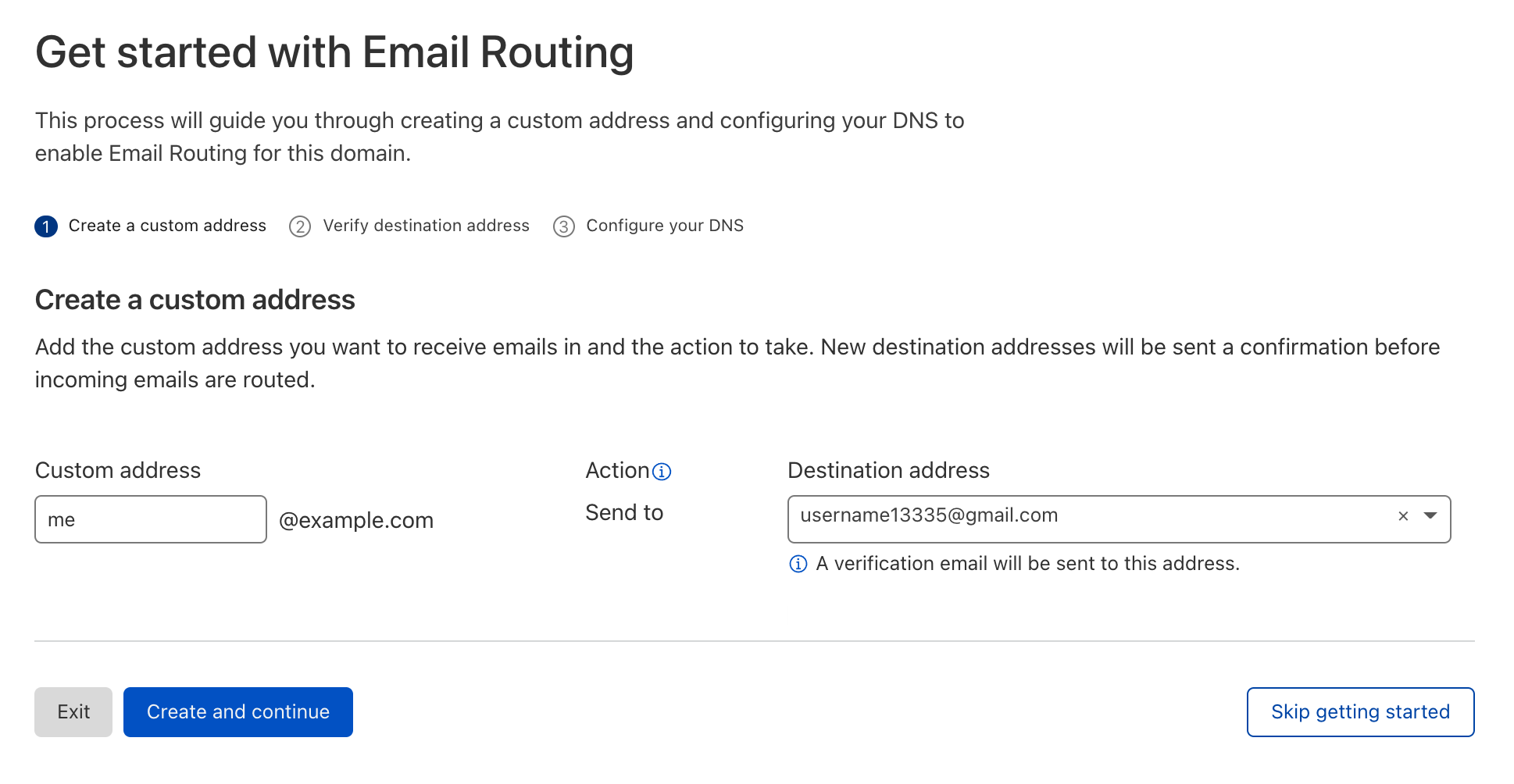
With Email Routing, you can effectively start receiving Emails in any of your domains for any number of custom addresses you want and forward the messages to any existing destination mailboxes. We will automatically set up everything for you, and you can have it running in minutes today, at no cost.

Here’s a step-by-step tutorial on how you can start receiving emails to example.com, forward them to Gmail (or any other email provider) at [email protected].

Using Cloudflare Email Routing with Gmail

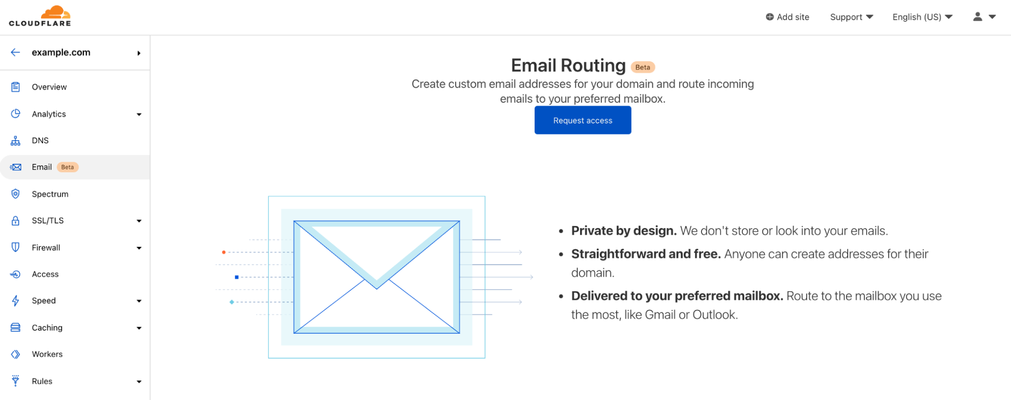
First, login to your Cloudflare Dashboard and select your example.com zone. Click “Email (Beta)” in the left navigation panel, and request to join the Beta program.

Today it still takes a couple of days to get approved into the beta, but feel free to ping us on the Discord server or community forum if you can’t wait.

Migrating to Cloudflare Email Routing

Once you get invited to join Email Routing, we will take you to our three-step easy configuration wizard. The first step is to define the custom address [email protected] and the destination address [email protected]. Don’t worry too much, you can modify or add others later.

Migrating to Cloudflare Email Routing

This step will trigger sending a confirmation email to [email protected] so that we can prove that the destination Inbox is yours. You need to open Gmail and press the verification link.

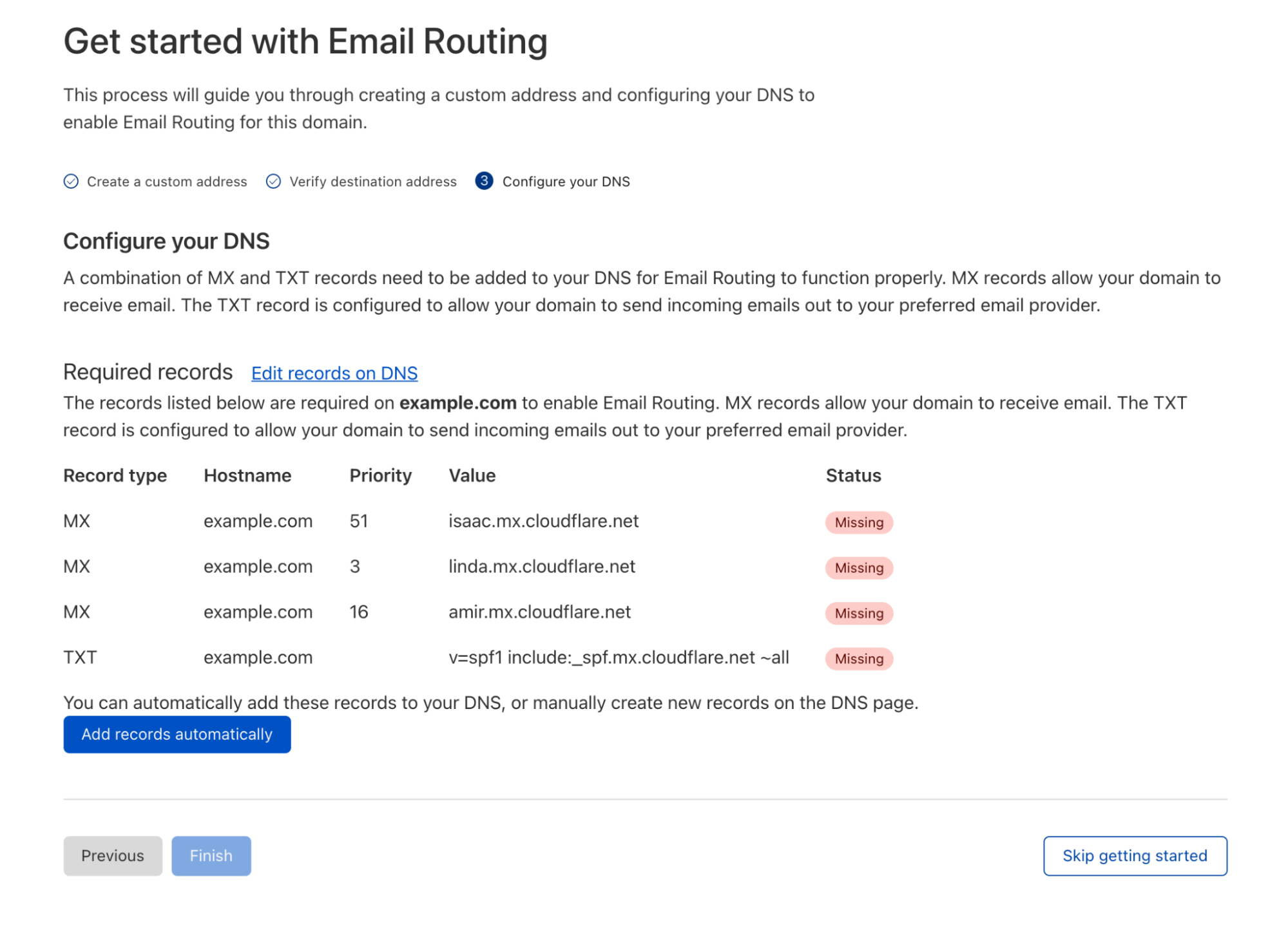
Then, on the last step, you need to configure your zone MX and SPF DNS records. We will do this automatically for you. Just press “Add records automatically“. If you already have MX or SPF configured, we will guide you through the conflicts we find and help you solve them.

Migrating to Cloudflare Email Routing

That’s it, Email Routing is now configured, and you can start sending emails to [email protected] and read them at [email protected] in Gmail.

Migrating to Cloudflare Email Routing

Gmail address conventions

Gmail and G suite, now Google Workspace, support two email address conventions that help organize your messages and fight spam.

The first one is the plus (“+”) sign. If you append a “+” sign and any combination of words after your email address, it will still get delivered to your inbox. For example, you can use [email protected], and it will get delivered at [email protected] and automatically get tagged “finance”. You can then use this to set up filters in Gmail.

The second one is Gmail ignores dots (“.”) in addresses entirely. For instance, sending an email to [email protected], [email protected], or [email protected] is all the same.

If you want to use these conventions with Cloudflare Email Routing, you can. Enable the “Catch-all address” feature and forward every incoming address for which there’s no other rule configured to the verified destination address of your choice ([email protected] in this example).

Migrating to Cloudflare Email Routing

Conclusion

This is only one small example of what you can do with Email Routing today. We hope you find it helpful if you’re looking for a new home for your email. For more information see our documentation pages.

Email needs more innovation. We’re immensely excited about Email Routing and our ideas for it in the roadmap. Expect improved metrics and advanced routing options in our rules engine in the near future.

Feel free to join the Beta today and ping us in our Discord server or community forum if you can’t wait; we’ll do our best to prioritize the community requests before we open the service.

Why Security in Kubernetes Isn’t the Same as in Linux: Part 1

Post Syndicated from Sagi Rosenthal original https://blog.rapid7.com/2022/01/27/why-security-in-kubernetes-isnt-the-same-as-in-linux-part-1/

Why Security in Kubernetes Isn't the Same as in Linux: Part 1

Kubernetes was first presented in 2014, and it almost entirely changed the way technological and even non-tech companies use infrastructure for running their applications. The Kubernetes platform still feels new and exciting — it has awesome features and can fit most use cases.

But hackers find the combination of new technology and user inexperience that’s just right for their malicious activity. Deploying your product on a Kubernetes cluster has a different security cost than on a traditional Linux server.

What are the risks of using Kubernetes?

The risks of a Kubernetes (K8s) deployment are actually the same as in traditional Linux servers. Most of them can be summed up to these 3 targets:

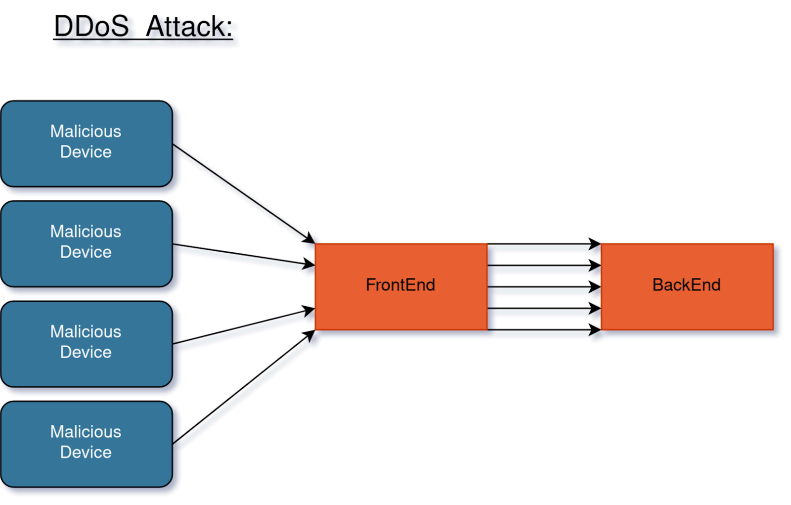
  • Denial of Service (DoS): These kinds of attacks want your service down. They can be caused in many different ways, including distributed denial of service (DDoS) attacks or SQL injections that erase your databases. As there is no direct profit to the attacker, these attacks are of most interest to malicious groups who disagree with your company values or products, or to your competitors.
Why Security in Kubernetes Isn't the Same as in Linux: Part 1
  • Information exfiltration: Another type of attack targets the information you hold. These attacks can collect your information, like your profits, source codes, names of employees, and so on. Or they can collect private data about your customers and users — who they are, their credit card numbers, health state, financial assets, and everything you know about them. None of this is data you want to be known outside the company.
  • Hardware hijack: A hardware hijack is any type of attack that runs a malicious code on your compute resources and causes them to operate in a way that you did not program or intend them to run. Most of these attacks are related to cryptocurrency. They typically either turn your CPU/GPU to Bitcoin miner or conduct a ransomware attack by encrypting your file system and requesting you to pay ransom (usually in Bitcoin) to unencrypt it. As the important point here for attackers is profit, not the identity of the victim, these attacks usually originate from bots or automatic scripts, rather than with dedicated special operations of malicious groups or individuals.

How can you defend yourself?

Securing deployments and identifying malicious activity on Kubernetes clusters is similar to how it’s done on traditional Linux servers. Most of the differences are in the implementation itself. But there are some distinctions worth mentioning. Let’s focus in on the operating system aspects of security.

Processes and system calls

“The system call is the fundamental interface between an application and the Linux kernel.” —Linux manual page

Linux has over 400 different system calls. These can be used for requesting to read a file, executing another program, sending a network message, and more. As you’ve probably guessed, these operations can be risky when used by unwanted programs.

The Linux Kernel has security mechanisms against malware, but it isn’t fully protected. So system calls may seem legitimate even when they aren’t. Tracking these system calls can give good insight on what a process does. In native Linux, it can be easy to track these down from a single point on the server. However, in K8s Linux nodes, the distribution, dynamics, and containerization makes this mission a very complex task.

Network security

The internet connection is your face for the customers, but it’s also the entry point for various malicious software into your infrastructure. Luckily, the big cloud providers and most of the internet-facing frameworks are well-protected against these attacks. But nothing is 100% safe. Moreover, some of the images you are using may contain security holes themselves. These can cause a malicious program to initiate from inside your cluster.

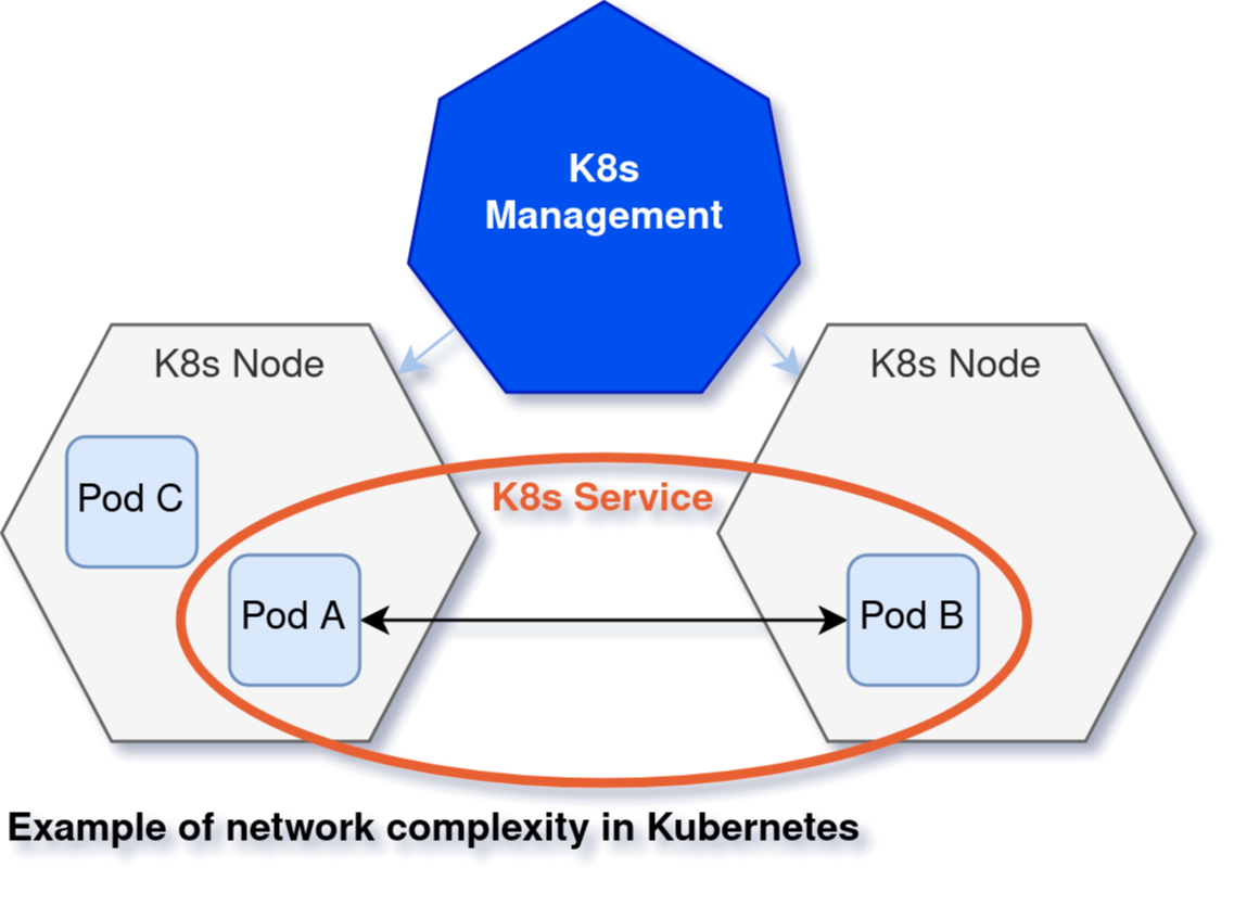
Tracking the network from the inside out can give you a lot of information on malicious activity. But you also have to consider the “east-to-west” traffic inside your infrastructure — the internal communication. In traditional Linux servers and VMs, you know exactly which microservices exist and define firewall services accordingly. However, in Kubernetes, the dynamic nature of the pods and resources makes it hard to track this traffic, so it can be difficult to find the network holes.

Why Security in Kubernetes Isn't the Same as in Linux: Part 1

File system

It may seem easy to detect new files and file changes in order to determine unwanted changes, but tracking and analyzing your whole file system can be a large, complex task in Linux servers. They can have terabytes of storage, and reading them — especially from a magnetic hard disk — isn’t fast enough to detect malicious activity when it happens. However, the containerization concept of Kubernetes can be to our advantage here, as container images are usually small, lightweight, and repetitive. Looking inside the containers files should have highly expected results.

More to come

This is one of two articles covering the detective resources that can help us identify unwanted activity in your Kubernetes clusters. In this first part, we saw that both Kubernetes and traditional Linux servers have vulnerabilities that originate in the processes, network, or file system. However, there are differences in how to monitor malicious activity in Kubernetes versus Linux. Some vulnerabilities may seem harder to defend in Kubernetes, but most of them are actually easier.

InsightCloudSec, Rapid7’s cloud-native security platform, covers these differences and ensures your on-premises server farm is secured.

The next article will explain further about the unique aspects of Kubernetes security that do not exist in traditional Linux servers. Stay tuned!

Additional reading

Kubernetes Guardrails: Bringing DevOps and Security Together on Cloud

Stay Ahead of Threats With Cloud Workload Protection

Make Room for Cloud Security in Your 2022 Budget

Time to Act: Bridging the Gap in Cloud Automation Adoption

NEVER MISS A BLOG

Get the latest stories, expertise, and news about security today.

Security updates for Thursday

Post Syndicated from original https://lwn.net/Articles/882882/rss

Security updates have been issued by CentOS (polkit), Debian (uriparser), Fedora (cryptsetup, flatpak, flatpak-builder, and polkit), Gentoo (polkit), Mageia (virtualbox), Red Hat (httpd24-httpd, httpd:2.4, and parfait:0.5), SUSE (clamav, log4j, python-numpy, and strongswan), and Ubuntu (vim).

The Roots project: Implementing culturally responsive computing teaching in schools in England

Post Syndicated from Sue Sentance original https://www.raspberrypi.org/blog/culturally-responsive-computing-teaching-schools-england-roots-research-project/

Since last year, we have been investigating culturally relevant pedagogy and culturally responsive teaching in computing education. This is an important part of our research to understand how to make computing accessible to all young people. We are now continuing our work in this area with a new project called Roots, bridging our research team here at the Foundation and the team at the Raspberry Pi Computing Education Research Centre, which we jointly created with the University of Cambridge in its Department of Computer Science and Technology.

Across both organisations, we’ve got great ambitions for the Centre, and I’m delighted to have been appointed as its Director. It’s a great privilege to lead this work. 

What do we mean by culturally relevant pedagogy?

Culturally relevant pedagogy is a framework for teaching that emphasises the importance of incorporating and valuing all learners’ knowledge, ways of learning, and heritage. It promotes the development of learners’ critical consciousness of the world and encourages them to ask questions about ethics, power, privilege, and social justice. Culturally relevant pedagogy emphasises opportunities to address issues that are important to learners and their communities.

Culturally responsive teaching builds on the framework above to identify a range of teaching practices that can be implemented in the classroom. These include:

  • Drawing on learners’ cultural knowledge and experiences to inform the curriculum
  • Providing opportunities for learners to choose personally meaningful projects and express their own cultural identities
  • Exploring issues of social justice and bias

The story so far

The overall objective of our work in this area is to further our understanding of ways to engage underrepresented groups in computing. In 2021, funded by a Special Projects Grant from ACM’s Special Interest Group in Computer Science Education (SIGCSE), we established a working group of teachers and academics who met up over the course of three months to explore and discuss culturally relevant pedagogy. The result was a collaboratively written set of practical guidelines about culturally relevant and responsive teaching for classroom educators.

The video below is an introduction for teachers who may not be familiar with the topic, showing the perspectives of three members of the working group and their students. You can also find other resources that resulted from this first phase of the work, and read our Special Projects Report.

We’re really excited that, having developed the guidelines, we can now focus on how culturally responsive computing teaching can be implemented in English schools through the Roots project, a new, related project supported by funding from Google. This funding continues Google’s commitment to grow the impact of computer science education in schools, which included a £1 million donation to support us and other organisations to develop online courses for teachers.

The next phase of work: Roots

In our new Roots project, we want to learn from practitioners how culturally responsive computing teaching can be implemented in classrooms in England, by supporting teachers to plan activities, and listening carefully to their experiences in school. Our approach is similar to the Research-Practice-Partnership (RPP) approach used extensively in the USA to develop research in computing education; this approach hasn’t yet been used in the UK. In this way, we hope to further develop and improve the guidelines with exemplars and case studies, and to increase our understanding of teachers’ motivations and beliefs with respect to culturally responsive computing teaching.

The pilot phase of the Roots project starts this month and will run until December 2022. During this phase, we will work with a small group of schools around London, Essex, and Cambridgeshire. Longer-term, we aim to scale up this work across the UK.

The project will be centred around two workshops held in participating teachers’ schools during the first half of the year. In the first workshop, teachers will work together with facilitators from the Foundation and the Raspberry Pi Computing Education Research Centre to discuss culturally responsive computing teaching and how to make use of the guidelines in adapting existing lessons and programmes of study. The second workshop will take place after the teachers have implemented the guidelines in their classroom, and it will be structured around a discussion of the teachers’ experiences and suggestions for iteration of the guidelines. We will also be using a visual research methodology to create a number of videos representing the new knowledge gleaned from all participants’ experiences of the project. We’re looking forward to sharing the results of the project later on in the year. 

We’re delighted that Dr Polly Card will be leading the work on this project at the Raspberry Pi Computing Education Research Centre, University of Cambridge, together with Saman Rizvi in the Foundation’s research team and Katie Vanderpere-Brown, Assistant Headteacher, Saffron Walden County High School, Essex and Computing Lead of the NCCE London, Hertfordshire and Essex Computing Hub.

More about equity, diversity, and inclusion in computing education

We hold monthly research seminars here at the Foundation, and in the first half of 2021, we invited speakers who focus on a range of topics relating to equity, diversity, and inclusion in computing education.

As well as holding seminars and building a community of interested people around them, we share the insights from speakers and attendees through video recordings of the sessions, blog posts, and the speakers’ presentation slides. We also publish a series of seminar proceedings with referenced chapters written by the speakers.

You can download your copy of the proceedings of the equity, diversity, and inclusion series now.  

The post The Roots project: Implementing culturally responsive computing teaching in schools in England appeared first on Raspberry Pi.

New – Amazon EC2 X2iezn Instances Powered by the Fastest Intel Xeon Scalable CPU for Memory-Intensive Workloads

Post Syndicated from Channy Yun original https://aws.amazon.com/blogs/aws/new-amazon-ec2-x2iezn-instances-powered-by-the-fastest-intel-xeon-scalable-cpu-for-memory-intensive-workloads/

Electronic Design Automation (EDA) workloads require high computing performance and a large memory footprint. These workloads are sensitive to faster CPU performance and higher clock speeds since the faster performance allows more jobs to be completed on the lower number of cores. At AWS re:Invent 2020, we launched Amazon EC2 M5zn instances which use second-generation Intel Xeon Scalable (Cascade Lake) processors with an all-core turbo clock frequency of up to 4.5 GHz, which is the fastest of any cloud instance.

Our customers have enjoyed the high single-threaded performance, high-speed networking, and balanced memory-to-vCPU ratio of EC2 M5zn instances. They have asked for instances that will leverage these features while also providing them a greater memory footprint per vCPU.

Today, we are launching Amazon EC2 X2iezn instances, which use the same Intel Xeon Scalable processors as M5zn instances, with an all-core turbo clock frequency of 4.5 GHz and up to 1.5 TiB of memory, which is the fastest of any cloud instance for EDA workloads. These instances are capable of delivering up to 55 percent better price-performance per vCPU compared to X1e instances.

X2iezn instances offer 32 GiB of memory per vCPU and will support up to 48 vCPUs and 1536 GiB of memory. Built on the AWS Nitro, they deliver up to 100 Gbps of networking bandwidth and 19 Gbps of dedicated Amazon EBS bandwidth to improve performance for EDA applications.

You might have noticed that we’re now using the “i” suffix in the instance type to specify that the instances are using an Intel processor, “e” in the memory-optimized instance family to indicate extended memory, “z” which indicates high-frequency processors, and “n” to support higher network bandwidth up to 100 Gbps.

X2iezn instances are VPC only, HVM-only, and EBS-Optimized, with support for Optimize vCPU. As you can see, the memory-to-vCPU ratio on these instances is the same as that of previous-generation X1e instances:

Instance Name vCPUs RAM (GiB) Network Bandwidth (Gbps) EBS-Optimized Bandwidth (Gbps)
x2iezn.2xlarge 8 256 Up to 25 3.170
x2iezn.4xlarge 16 512 Up to 25 4.750
x2iezn.6xlarge 24 768 50 9.5
x2iezn.8xlarge 32 1024 75 12
x2iezn.12xlarge 48 1536 100 19
x2iezn.metal 48 1536 100 19

Many customers will be able to benefit from using X2iezn instances to improve performance and efficiency for their EDA workloads. Here are some examples:

  • Annapurna Labs tested the X2iezn instances with Calibre’s Design Rule Checking, which has shown a 40 percent faster runtime compared to X1e instances, and a 25 percent faster runtime over R5d instances.
  • Astera Labs is a fabless, cloud-based semiconductor company developing purpose-built CXL, PCIe, and Ethernet connectivity solutions for data-centric systems. They were able to see performance gains of up to 25 percent compared to similar EDA workloads running on R5 instances.
  • Cadence tested the X2iezn instances using their Pegasus True Cloud feature, which allows designers to run physical verification jobs on the cloud and observed a 50 percent performance improvement over R5 instances. They see X2iezn instances as an excellent environment for testing EDA workloads.
  • NXP Semiconductors worked with AWS to run their Calibre and Spectre workloads on Amazon EC2 X2iezn instances, which measured 10-15 percent higher performance using X2iezn instances compared to their on-premises, Xeon Gold 6254 with max turbo frequency of 4.0GHz.
  • Siemens EDA worked with AWS to test the new Amazon EC2 X2iezn HPC/EDA focused instances with the industry performance and sign-off leader Calibre evaluating advanced node DRC workloads. They were pleased to demonstrate performance improvements of up to 14% using the 4.5 GHz all core turbo frequency of X2iezn instances for all VMs in the run. Additionally, they successfully demonstrated the use of a heterogeneous server configuration using the X2iezn as the primary node and other lower memory VMs for remote compute – providing an 11% speed up and attractive value. These results confirmed the X2iezn is a good fit for primary server EDA workloads for Calibre Physical and Circuit verification applications.
  • Synopsys IC Validator provides highly scalable high-performance physical verification signoff. They achieved 15 percent performance improvement, scalability to 1000s of cores, and 30 percent better efficiency using IC Validator’s unique elastic CPU management technology versus R5d instances.

Things to Know
Here are some fun facts about the X2iezn instances:

Optimizing CPU—You can disable Intel Hyper-Threading Technology for workloads that perform well with single-threaded CPUs, like some HPC applications.

NUMA—You can make use of non-uniform memory access (NUMA) on x2iezn.12xlarge instances. This advanced feature is worth exploring if you have a deep understanding of your application’s memory access patterns.

Available Now
Amazon EC2 X2iezn instances are now available in the US East (N. Virginia), US West (Oregon), Asia Pacific (Tokyo), and Europe (Ireland) Regions. You can use On-Demand Instances, Reserved Instances, Savings Plan, and Spot Instances. Dedicated Instances and Dedicated Hosts are also available.

To learn more, visit our EC2 X2i Instances page, and please send feedback to the AWS forum for EC2 or through your usual AWS Support contacts.

– Channy

[$] Goodbye FLoC, hello Topics

Post Syndicated from original https://lwn.net/Articles/882607/rss

Back in May, we looked at a Google proposal
to replace third-party
cookies
with something called the
“Federated Learning of Cohorts”
(FLoC). Third-party cookies were once used to track users all over the web
so that advertisers could, supposedly, target their ads better, but, of the
major browsers, only Google’s Chrome browser fails to block them today. Google
took a fair amount of flak for FLoC, since it was not perceived to be much
of a win for users’ privacy—and was mostly a sop to the (Google-dominated)
web-advertising industry. Now the company is back with a different
proposal that could, eventually, replace third-party cookies in Chrome: Topics.

Incorrect proxying of 24 hostnames on January 24, 2022

Post Syndicated from Jeremy Hartman original https://blog.cloudflare.com/incorrect-proxying-of-24-hostnames-on-january-24-2022/

Incorrect proxying of 24 hostnames on January 24, 2022

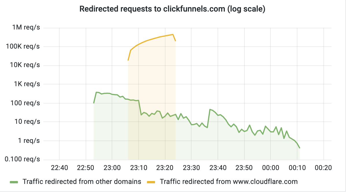
On January 24, 2022, as a result of an internal Cloudflare product migration, 24 hostnames (including www.cloudflare.com) that were actively proxied through the Cloudflare global network were mistakenly redirected to the wrong origin. During this incident, traffic destined for these hostnames was passed through to the clickfunnels.com origin and may have resulted in a clickfunnels.com page being displayed instead of the intended website. This was our doing and clickfunnels.com was unaware of our error until traffic started to reach their origin.

API calls or other expected responses to and from these hostnames may not have responded properly, or may have failed completely. For example, if you were making an API call to api.example.com, and api.example.com was an impacted hostname, you likely would not have received the response you would have expected.

Here is what happened:

At 2022-01-24 22:24 UTC we started a migration of hundreds of thousands of custom hostnames to the Cloudflare for SaaS product. Cloudflare for SaaS allows SaaS providers to manage their customers’ websites and SSL certificates at scale – more information is available here. This migration was intended to be completely seamless, with the outcome being enhanced features and security for our customers. The migration process was designed to read the custom hostname configuration from a database and migrate it from SaaS v1 (the old system) to SaaS v2 (the current version) automatically.

To better understand what happened next, it’s important to explain a bit more about how custom hostnames are configured.

First, Cloudflare for SaaS customers can configure any hostname; but before we will proxy traffic to them, they must prove (via DNS validation) that they actually are allowed to handle that hostname’s traffic.

When the Cloudflare for SaaS customer first configures the hostname, it is marked as pending until DNS validation has occurred. Pending hostnames are very common for Cloudflare for SaaS customers as the hostname gets provisioned, and then the SaaS provider will typically work with their customer to put in place the appropriate DNS validation that proves ownership.

Once a hostname passes DNS validation, it moves from a pending state to an active state and can be proxied. Except in one case: there’s a special check for whether the hostname is marked as blocked within Cloudflare’s system. A blocked hostname is one that can’t be activated without manual approval by our Trust & Safety team. Some scenarios that could lead to a hostname being blocked include when the hostname is a Cloudflare-owned property, a well known brand, or a hostname in need of additional review for a variety of reasons.

During this incident, a very small number of blocked hostnames were erroneously moved to the active state while migrating clickfunnels.com’s customers. Once that occurred, traffic destined for those previously blocked hostnames was then processed by a configuration belonging to clickfunnels.com, sending traffic to the clickfunnels.com’s origin. One of those hostnames was www.cloudflare.com. Note that it was www.cloudflare.com and not cloudflare.com, so subdomains like dash.cloudflare.com, api.cloudflare.com, cdnjs.cloudflare.com, and so on were unaffected by this problem.

As the migration process continued down the list of hostnames, additional traffic was re-routed to the clickfunnels.com origin. At 23:06 UTC www.cloudflare.com was affected. At 23:15 UTC an incident was declared internally. Since the first alert we received was for www.cloudflare.com, we started our investigation there. In the next 19 minutes, the team restored www.cloudflare.com to its correct origin, determined the breadth of the impact and the root cause of the incident, and began remediation for the remaining affected hostnames.

By 2022-01-25 00:13 UTC, all custom hostnames had been restored to their proper configuration and the incident was closed. We have contacted all the customers who were affected by this error. We have worked with ClickFunnels to delete logs of this event to ensure that no data erroneously sent to the clickfunnels.com’s origin is retained by them and are very grateful for their speedy assistance.

Here is a graph (on a log scale) of requests to clickfunnels.com during the event. Out of a total of 268,430,157 requests redirected, 268,220,296 (99.92%) were for www.cloudflare.com:

Incorrect proxying of 24 hostnames on January 24, 2022

At Cloudflare, we take these types of incidents very seriously, dedicating massive amounts of resources in preventative action and in follow-up engineering. In this case, there are both procedural and technical follow-ups to prevent reoccurrence. Here are our next steps:

  • No more blocked hostname overrides. All blocked hostname changes will route through our verification pipeline as part of the migration process.
  • All migrations will require explicit validation and approval from SaaS customers for a blocked hostname to be considered for activation.
  • Additional monitoring will be added to the hostnames being migrated to spot potential erroneous traffic patterns and alert the migration team.
  • Additional monitoring added for www.cloudflare.com.
  • Stage hostname activations on non-production elements prior to promoting to production will enable the ability to verify the new hostname state is expected. This will allow us to catch issues before they hit production traffic.

Conclusion

This event exposed previously unknown gaps in our process and technology that directly impacted our customers. We are truly sorry for the disruption to our customers and any potential visitor to the impacted properties. Our commitment is to provide fully reliable and secure products, and we will continue to make every effort possible to deliver just that for our customers and partners.

Let’s Architect! Architecture and Sustainability

Post Syndicated from Luca Mezzalira original https://aws.amazon.com/blogs/architecture/lets-architect-1-architecture-and-sustainability/

We often read news about sustainability and how governments and large corporations are working to build a better world for the future. But, have you ever asked yourself what you can do? As a software architect, how can you make a difference by addressing sustainability challenges?

In this first post of Let’s Architect!, a series of posts that gathers content to help software architects and tech leaders explore new ideas, case studies, and technical approaches, we provide materials to help you design sustainable architectures and create awareness on sustainability.

Optimizing your AWS Infrastructure for Sustainability

How do you optimize the compute layer of your environment from a sustainability perspective? An idle server still consumes power, and regulating its power consumption is one way to improve environmental impact. But, the cloud offers many other metrics and features to monitor and optimize your system.

This blog post shows you how to analyze the utilization of your compute resources, explains the main features to automatically scale based on demand, and highlights how serverless can optimize your resource utilization. Knowing how to use your resources efficiently will help reduce the amount of energy spent by your workload.

The shared responsibility model for sustainability shows how it is a shared responsibility between AWS and customers

The shared responsibility model for sustainability shows how it is a shared responsibility between AWS and customers

Building Sustainably on AWS

This talk provides several best practices you can follow as to design more sustainable architectures. It gives different tips to integrate sustainable practices throughout business operations and provides some guardrails that could help you achieve your organization’s sustainability goals more quickly.

Luke Hargreaves explaining how to build sustainably on AWS

Luke Hargreaves explaining how to build sustainably on AWS

Moving to event-driven architectures

An efficient architecture is typically a more sustainable architecture. This video explains how Amazon.com approaches event-driven architectures.

Event-driven architectures use events to communicate across different microservices. This architectural pattern works to reduce bandwidth consumption and CPU utilization and potentially lower cost. By choosing a serverless event-driven architecture, you’ll optimize your overall resource utilization because the code is run in response to events.

Tim Bray presenting how to move to an event-driven architecture at re:Invent 2019

Tim Bray presenting how to move to an event-driven architecture at re:Invent 2019

Supporting climate model simulations to accelerate climate science

This blog post discusses how collaborating research teams use the data generated through climate model simulations to study impacts on Earth and human systems—including agriculture, drought, flooding, and human health—in various parts of the world.
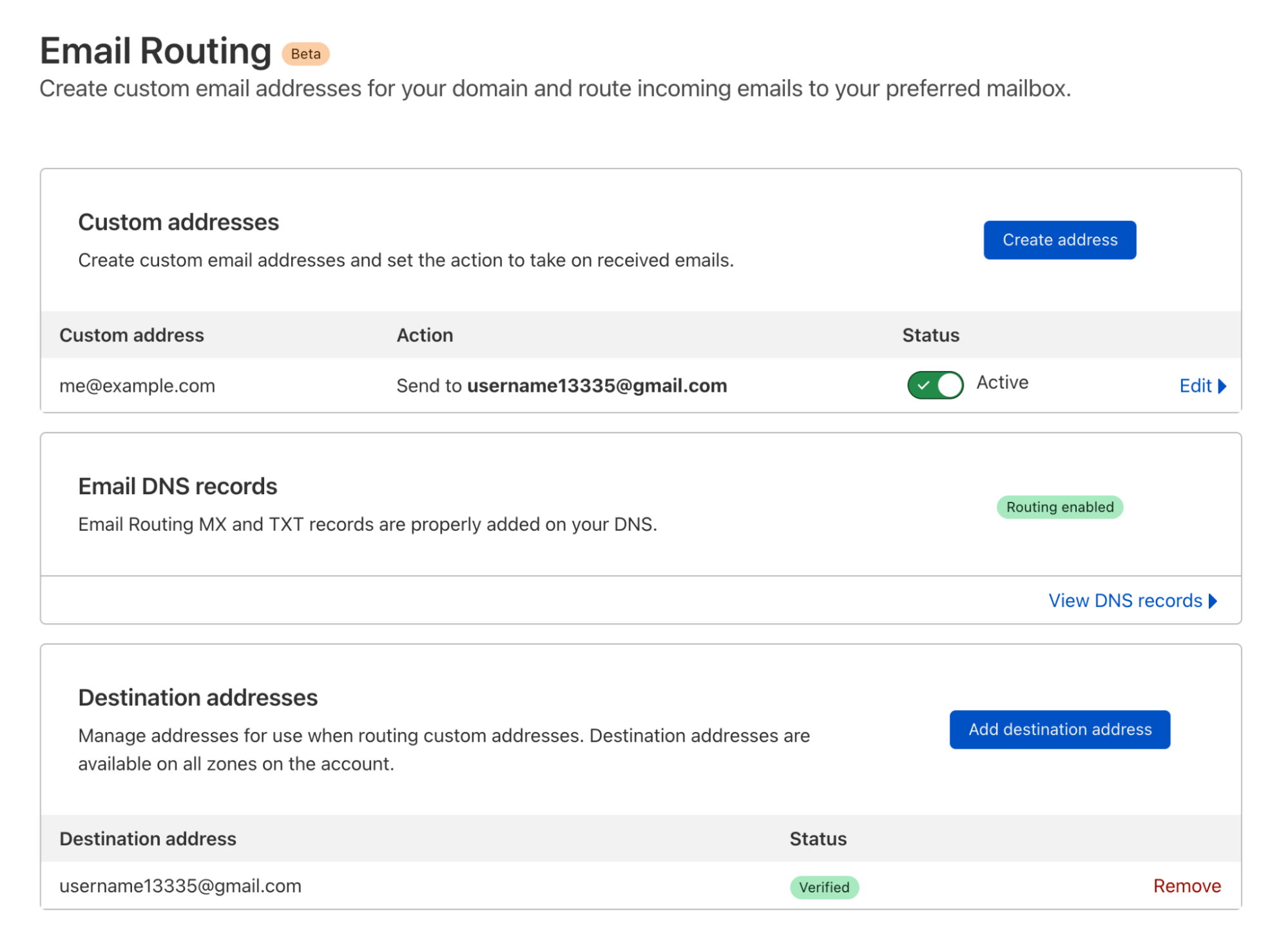
These studies will advance understanding of near-term climate and climate-intervention responses, and accelerate progress on a time-sensitive problem for humanity.

This architecture built on AWS Parallel Cluster supports weather and climate modeling workloads

This architecture built on AWS ParallelCluster supports weather and climate modeling workloads

See you next time!

Thanks for reading! If you want to deep dive into the topic of sustainability even more, don’t miss the Architecture Monthly edition on Sustainability.

See you in a couple of weeks when we discuss novel ways to use machine learning and artificial intelligence!

Looking for more architecture content? AWS Architecture Center provides reference architecture diagrams, vetted architecture solutions, Well-Architected best practices, patterns, icons, and more!

New DeadBolt Ransomware Targets NAT Devices

Post Syndicated from Bruce Schneier original https://www.schneier.com/blog/archives/2022/01/new-deadbolt-ransomware-targets-nat-devices.html

There’s a new ransomware that targets NAT devices made by QNAP:

The attacks started today, January 25th, with QNAP devices suddenly finding their files encrypted and file names appended with a .deadbolt file extension.

Instead of creating ransom notes in each folder on the device, the QNAP device’s login page is hijacked to display a screen stating, “WARNING: Your files have been locked by DeadBolt”….

[…]

BleepingComputer is aware of at least fifteen victims of the new DeadBolt ransomware attack, with no specific region being targeted.
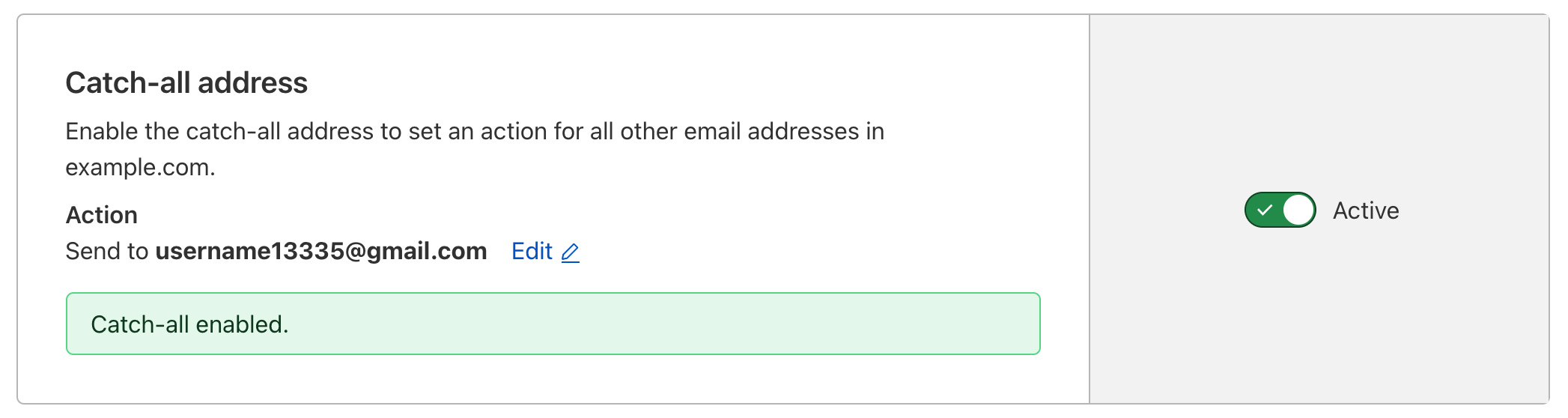
As with all ransomware attacks against QNAP devices, the DeadBolt attacks only affect devices accessible to the Internet.

As the threat actors claim the attack is conducted through a zero-day vulnerability, it is strongly advised that all QNAP users disconnect their devices from the Internet and place them behind a firewall.

Security updates for Wednesday

Post Syndicated from original https://lwn.net/Articles/882724/rss

Security updates have been issued by CentOS (httpd), Debian (libxfont, lrzsz, nss, openjdk-17, policykit-1, webkit2gtk, and wpewebkit), Mageia (polkit), openSUSE (expat, json-c, kernel, polkit, qemu, rust1.55, rust1.57, thunderbird, unbound, and webkit2gtk3), Oracle (httpd:2.4, java-11-openjdk, and polkit), Red Hat (httpd:2.4, OpenShift Container Platform 3.11.570, polkit, and Red Hat OpenStack Platform 16.1 (etcd)), Scientific Linux (polkit), Slackware (polkit), SUSE (aide, expat, firefox, json-c, kernel, polkit, qemu, rust, rust1.55, rust1.57, thunderbird, unbound, and webkit2gtk3), and Ubuntu (policykit-1 and xorg-server).

The collective thoughts of the interwebz