Stream data from relational databases to Amazon Redshift with upserts using AWS Glue streaming jobs

Post Syndicated from Noritaka Sekiyama original https://aws.amazon.com/blogs/big-data/stream-data-from-relational-databases-to-amazon-redshift-with-upserts-using-aws-glue-streaming-jobs/

Traditionally, read replicas of relational databases are often used as a data source for non-online transactions of web applications such as reporting, business analysis, ad hoc queries, operational excellence, and customer services. Due to the exponential growth of data volume, it became common practice to replace such read replicas with data warehouses or data lakes to have better scalability and performance. In most real-world use cases, it’s important to replicate the data from a source relational database to the target in real time. Change data capture (CDC) is one of the most common design patterns to capture the changes made in the source database and relay them to other data stores.

AWS offers a broad selection of purpose-built databases for your needs. For analytic workloads such as reporting, business analysis, and ad hoc queries, Amazon Redshift is powerful option. With Amazon Redshift, you can query and combine exabytes of structured and semi-structured data across your data warehouse, operational database, and data lake using standard SQL.

To achieve CDC from Amazon Relational Database Service (Amazon RDS) or other relational databases to Amazon Redshift, the simplest solution is to create an AWS Database Migration Service (AWS DMS) task from the database to Amazon Redshift. This approach works well for simple data replication. To have more flexibility to denormalize, transform, and enrich the data, we recommend using Amazon Kinesis Data Streams and AWS Glue streaming jobs between AWS DMS tasks and Amazon Redshift. This post demonstrates how this second approach works in a customer scenario.

Example use case

For our example use case, we have a database that stores data of a fictional organization that holds sports events. We have three dimension tables: sport_event, ticket, and customer, and one fact table: ticket_activity. The table sport_event stores sport type (such as baseball or football), date, and location. The table ticket stores seat level, location, and ticket policy for the target sport event. The table customer stores individual customer names, email addresses, and phone numbers, which are sensitive information. When a customer buys a ticket, the activity (e.g. who purchased the ticket) is recorded in the table ticket_activity. One record is inserted into the table ticket_activity every time a customer buys a ticket, so new records are being ingested into this fact table continuously. The records ingested into the table ticket_activity are only updated when needed, when an administrator maintains the data.

We assume a persona, a data analyst, who is responsible for analyzing trends of the sports activity from this continuous data in real time. To use Amazon Redshift as a primary data mart, the data analyst needs to enrich and clean the data so that users like business analysts can understand and utilize the data easily.

The following are examples of the data in each table.

The following is the dimension table sport_event.

event_id sport_type start_date location
1 35 Baseball 9/1/2021 Seattle, US
2 36 Baseball 9/18/2021 New York, US
3 37 Football 10/5/2021 San Francisco, US

The following is the dimension table ticket (the field event_id is the foreign key for the field event_id in the table sport_event).

ticket_id event_id seat_level seat_location ticket_price
1 1315 35 Standard S-1 100
2 1316 36 Standard S-2 100
3 1317 37 Premium P-1 300

The following is the dimension table customer.

customer_id name email phone
1 222 Teresa Stein [email protected] +1-296-605-8486
2 223 Caleb Houston [email protected] 087-237-9316×2670
3 224 Raymond Turner [email protected] +1-786-503-2802×2357

The following is the fact table ticket_activity (the field purchased_by is the foreign key for the field customer_id in the table customer).

ticket_id purchased_by created_by updated_by
1 1315 222 8/15/2021 8/15/2021
2 1316 223 8/30/2021 8/30/2021
3 1317 224 8/31/2021 8/31/2021

To make the data easy to analyze, the data analyst wants to have only one table that includes all the information instead of joining all four tables every time they want to analyze. They also want to mask the field phone_number and tokenize the field email_address as sensitive information. To meet this requirement, we merge these four tables into one table and denormalize, tokenize, and mask the data.

The following is the destination table for analysis, sport_event_activity.

ticket_id event_id sport_type start_date location seat_level seat_location ticket_price purchased_by name email_address phone_number created_at updated_at
1 1315 35 Baseball 9/1/2021 Seattle, USA Standard S-1 100 222 Teresa Stein 990d081b6a420d04fbe07dc822918c7ec3506b12cd7318df7eb3af6a8e8e0fd6 +*-***-***-**** 8/15/2021 8/15/2021
2 1316 36 Baseball 9/18/2021 New York, USA Standard S-2 100 223 Caleb Houston c196e9e58d1b9978e76953ffe0ee3ce206bf4b88e26a71d810735f0a2eb6186e ***-***-****x**** 8/30/2021 8/30/2021
3 1317 37 Football 10/5/2021 San Francisco, US Premium P-1 300 224 Raymond Turner 885ff2b56effa0efa10afec064e1c27d1cce297d9199a9d5da48e39df9816668 +*-***-***-****x**** 8/31/2021 8/31/2021

Solution overview

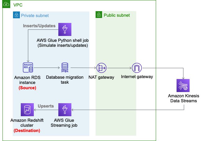
The following diagram depicts the architecture of the solution that we deploy using AWS CloudFormation.

We use an AWS DMS task to capture the changes in the source RDS instance, Kinesis Data Streams as a destination of the AWS DMS task CDC replication, and an AWS Glue streaming job to read changed records from Kinesis Data Streams and perform an upsert into the Amazon Redshift cluster. In the AWS Glue streaming job, we enrich the sports-event records.

Set up resources with AWS CloudFormation

This post includes a CloudFormation template for a quick setup. You can review and customize it to suit your needs.

The CloudFormation template generates the following resources:

  • An Amazon RDS database instance (source).
  • An AWS DMS replication instance, used to replicate the table ticket_activity to Kinesis Data Streams.
  • A Kinesis data stream.
  • An Amazon Redshift cluster (destination).
  • An AWS Glue streaming job, which reads from Kinesis Data Streams and the RDS database instance, denormalizes, masks, and tokenizes the data, and upserts the records into the Amazon Redshift cluster.
  • Three AWS Glue Python shell jobs:
    • rds-ingest-data-initial-<CloudFormation Stack name> creates four source tables on Amazon RDS and ingests the initial data into the tables sport_event, ticket, and customer. Sample data is automatically generated at random by Faker library.
    • rds-ingest-data-incremental-<CloudFormation Stack name> ingests new ticket activity data into the source table ticket_activity on Amazon RDS continuously. This job simulates customer activity.
    • rds-upsert-data-<CloudFormation Stack name> upserts specific records in the source table ticket_activity on Amazon RDS. This job simulates administrator activity.
  • AWS Identity and Access Management (IAM) users and policies.
  • An Amazon VPC, a public subnet, two private subnets, an internet gateway, a NAT gateway, and route tables.
    • We use private subnets for the RDS database instance, AWS DMS replication instance, and Amazon Redshift cluster.
    • We use the NAT gateway to have reachability to pypi.org to use MySQL Connector for Python from the AWS Glue Python shell jobs. It also provides reachability to Kinesis Data Streams and an Amazon Simple Storage Service (Amazon S3) API endpoint.

The following diagram illustrates this architecture.
To set up these resources, you must have the following prerequisites:

To launch the CloudFormation stack, complete the following steps:

  1. Sign in to the AWS CloudFormation console.
  2. Choose Launch Stack:
  3. Choose Next.
  4. For S3BucketName, enter the name of your new S3 bucket.
  5. For VPCCIDR, enter the CIDR IP address range that doesn’t conflict with your existing networks.
  6. For PublicSubnetCIDR, enter the CIDR IP address range within the CIDR you gave in VPCCIDR.
  7. For PrivateSubnetACIDR and PrivateSubnetBCIDR, enter the CIDR IP address range within the CIDR you gave for VPCCIDR.
  8. For SubnetAzA and SubnetAzB, choose the subnets you want to use.
  9. For DatabaseUserName, enter your database user name.
  10. For DatabaseUserPassword, enter your database user password.
  11. Choose Next.
  12. On the next page, choose Next.
  13. Review the details on the final page and select I acknowledge that AWS CloudFormation might create IAM resources with custom names.
  14. Choose Create stack.

Stack creation can take about 20 minutes.

Ingest new records

In this section, we walk you through the steps to ingest new records.

Set up an initial source table

To set up an initial source table in Amazon RDS, complete the following steps:

  1. On the AWS Glue console, choose Jobs.
  2. Select the job rds-ingest-data-initial-<CloudFormation stack name>.
  3. On the Actions menu, choose Run job.
  4. Wait for the Run status to show as SUCCEEDED.

This AWS Glue job creates a source table event on the RDS database instance.

Start data ingestion to the source table on Amazon RDS

To start data ingestion to the source table on Amazon RDS, complete the following steps:

  1. On the AWS Glue console, choose Triggers.
  2. Select the trigger periodical-trigger-<CloudFormation stack name>.
  3. On the Actions menu, choose Activate trigger.
  4. Choose Enable.

This trigger runs the job rds-ingest-data-incremental-<CloudFormation stack name> to ingest one record every minute.

Start data ingestion to Kinesis Data Streams

To start data ingestion from Amazon RDS to Kinesis Data Streams, complete the following steps:

  1. On the AWS DMS console, choose Database migration tasks.
  2. Select the task rds-to-kinesis-<CloudFormation stack name> .
  3. On the Actions menu, choose Restart/Resume.
  4. Wait for the Status to show as Load complete, replication ongoing.

The AWS DMS replication task ingests data from Amazon RDS to Kinesis Data Streams continuously.

Start data ingestion to Amazon Redshift

Next, to start data ingestion from Kinesis Data Streams to Amazon Redshift, complete the following steps:

  1. On the AWS Glue console, choose Jobs.
  2. Select the job streaming-cdc-kinesis2redshift-<CloudFormation stack name>.
  3. On the Actions menu, choose Run job.
  4. Choose Run job again.

This AWS Glue streaming job is implemented based on the guidelines in Updating and inserting new data. It performs the following actions:

  • Creates a staging table on the Amazon Redshift cluster using the Amazon Redshift Data API
  • Reads from Kinesis Data Streams, and creates a DataFrame with filtering only INSERT and UPDATE records
  • Reads from three dimension tables on the RDS database instance
  • Denormalizes, masks, and tokenizes the data
  • Writes into a staging table on the Amazon Redshift cluster
  • Merges the staging table into the destination table
  • Drops the staging table

After about 2 minutes from starting the job, the data should be ingested into the Amazon Redshift cluster.

Validate the ingested data

To validate the ingested data in the Amazon Redshift cluster, complete the following steps:

  1. On the Amazon Redshift console, choose EDITOR in the navigation pane.
  2. Choose Connect to database.
  3. For Connection, choose Create a new connection.
  4. For Authentication, choose Temporary credentials.
  5. For Cluster, choose the Amazon Redshift cluster cdc-sample-<CloudFormation stack name>.
  6. For Database name, enter dev.
  7. For Database user, enter the user that was specified in the CloudFormation template (for example, dbmaster).
  8. Choose Connect.
  9. Enter the query SELECT * FROM sport_event_activity and choose Run.

Now you can see the ingested records in the table sport_event_activity on the Amazon Redshift cluster. Let’s note the value of ticket_id from one of the records. For this post, we choose 1317 as an example.

Update existing records

Your Amazon Redshift cluster now has the latest data ingested from the tables on the source RDS database instance. Let’s update the data in the source table ticket_activity on the RDS database instance to see that the updated records are replicated to the Amazon Redshift cluster side.

The CloudFormation template creates another AWS Glue job. This job upserts the data with specific IDs on the source table event. To upsert the records in the source table, complete the following steps:

  1. On the AWS Glue console, choose Jobs.
  2. Choose the job rds-upsert-data-<CloudFormation stack name>.
  3. On the Actions menu, choose Edit job.
  4. Under Security configuration, script libraries, and job parameters (optional), for Job parameters, update the following parameters:
    1. For Key, enter --ticket_id_to_be_updated.
    2. For Value, replace 1 with one of the ticket IDs you observed on the Amazon Redshift console.
  5. Choose Save.
  6. Choose the job rds-upsert-data-<CloudFormation stack name>.
  7. On the Actions menu, choose Run job.
  8. Choose Run job.

This AWS Glue Python shell job simulates a customer activity to buy a ticket. It updates a record in the source table ticket_activity on the RDS database instance using the ticket ID passed in the job argument --ticket_id_to_be_updated. It automatically selects one customer, updates the field purchased_by with the customer ID, and updates the field updated_at with the current timestamp.

To validate the ingested data in the Amazon Redshift cluster, run the same query SELECT * FROM sport_event_activity. You can filter the record with the ticket_id value you noted earlier.

According to the rows returned to the query, the record ticket_id=1317 has been updated. The field updated_at has been updated from 2021-08-16 06:05:01 to 2021-08-16 06:53:52, and the field purchased_by has been updated from 449 to 14. From this result, you can see that this record has been successfully updated on the Amazon Redshift cluster side as well. You can also choose Queries in the left pane to see past query runs.

Clean up

Now to the final step, cleaning up the resources.

  1. Stop the AWS DMS replication task rds-to-kinesis-<CloudFormation stack name>.
  2. Stop the AWS Glue streaming job streaming-cdc-kinesis2redshift-<CloudFormation stack name>.
  3. Delete the CloudFormation stack.

Conclusion

In this post, we demonstrated how you can stream data—not only new records, but also updated records from relational databases—to Amazon Redshift. With this approach, you can easily achieve upsert use cases on Amazon Redshift clusters. In the AWS Glue streaming job, we demonstrated the common technique to denormalize, mask, and tokenize data for real-world use cases.


About the Authors

Noritaka Sekiyama is a Principal Big Data Architect on the AWS Glue team. He enjoys collaborating with different teams to deliver results like this post. In his spare time, he enjoys playing video games with his family.

Roman Gavrilov is an Engineering Manager at AWS Glue. He has over a decade of experience building scalable Big Data and Event-Driven solutions. His team works on Glue Streaming ETL to allow near real time data preparation and enrichment for machine learning and analytics.

Announcing Rust 1.56.0 and Rust 2021

Post Syndicated from original https://lwn.net/Articles/873655/rss

The Rust language project has announced the release of stable version 1.56.0 and the Rust 2021 edition.

We wrote about plans for the Rust 2021 Edition in May. Editions are a mechanism for opt-in changes that may otherwise pose backwards compatibility risk. See the edition guide for details on how this is achieved. This is a smaller edition, especially compared to 2018, but there are still some nice quality-of-life changes that require an edition opt-in to avoid breaking some corner cases in existing code.

See the detailed
release notes for 1.56.0 for lots more information on the release.

Swiftly Search Metadata with an Amazon S3 Serverless Architecture

Post Syndicated from Jiwan Panjiker original https://aws.amazon.com/blogs/architecture/swiftly-search-metadata-with-an-amazon-s3-serverless-architecture/

As you increase the number of objects in Amazon Simple Storage Service (Amazon S3), you’ll need the ability to search through them and quickly find the information you need.

In this blog post, we offer you a cost-effective solution that uses a serverless architecture to search through your metadata. Using a serverless architecture helps you reduce operational costs because you only pay for what you use.

Our solution is built with Amazon S3 event notifications, AWS Lambda, AWS Glue Catalog, and Amazon Athena. These services allow you to search thousands of objects in an S3 bucket by filenames, object metadata, and object keys. This solution maintains an index in an Apache Parquet file, which optimizes Athena queries to search Amazon S3 metadata. Using this approach makes it straightforward to run queries as needed without the need to ingest data or manage any servers.

Using Athena to search Amazon S3 objects

Amazon S3 stores and retrieves objects for a range of use cases, such as data lakes, websites, cloud-native applications, backups, archive, machine learning, and analytics. When you have an S3 bucket with thousands of files in it, how do you search for and find what you need? The object search box within the Amazon S3 user interface allows you to search by prefix, or you can search using Amazon S3 API’s LIST operation, which only returns 1,000 objects at a time.

A common solution to this issue is to build an external index and search for Amazon S3 objects using the external index. The Indexing Metadata in Amazon Elasticsearch Service Using AWS Lambda and Python and Building and Maintaining an Amazon S3 Metadata Index without Servers blog posts show you how to build this solution with Amazon OpenSearch Service or Amazon DynamoDB.

Our solution stores the external index in Amazon S3 and uses Athena to search the index. Athena makes it straightforward to search Amazon S3 objects without the need to manage servers or introduce another data repository. In the next section, we’ll talk about a few use cases where you can apply this solution.

Metadata search use cases

When your clients upload files to their S3 buckets, you’ll sometimes need to verify the files that were uploaded. You must validate whether you have received all the required information, including metadata such as customer identifier, category, received date, etc. The following examples will make use of this metadata:

  • Searching for a file from a specific date (or) date range
  • Finding all objects uploaded by a given customer identifier
  • Reviewing files for a particular category

The next sections outline how to build a serverless architecture to apply to use cases like these.

Building a serverless file metadata search on AWS

Let’s go through layers that are involved in our serverless architecture solution:

  1. Data ingestion: Set object metadata when objects are uploaded into Amazon S3. This layer uploads objects using the Amazon S3 console, AWS SDK, REST API, and AWS CLI.
  2. Data processing: Integrate Amazon S3 event notifications with Lambda to process S3 events. The AWS Data Wrangler library within Lambda will transform and build the metadata index file.
  3. Data catalog: Use AWS Glue Data Catalog as a central repository to store table definition and add/update business-relevant attributes of the metadata index. AWS Data Wrangler API creates the Apache Parquet files to maintain the AWS Glue Catalog.
  4. Metadata search: Define tables for your metadata and run queries using standard SQL with Athena to get started faster.

Reference architecture

Figure 1 illustrates our approach to implementing serverless file metadata search, which consists of the following steps:

  1. When you create new objects/files in an S3 bucket, the source bucket is configured with Amazon S3 Event Notification events (put, post, copy, etc.). Amazon S3 events provide the metadata information required for further processing and building the metadata index file on the destination bucket.
  2. The S3 event is sent to a Lambda function with necessary permissions on Amazon S3 using a resource-based policy. The Lambda function processes the event with metadata and converts it into an Apache Parquet file, which is then written into a target bucket. The AWS Data Wrangler API transforms and builds the metadata index file. The Lambda layer configures AWS Data Wrangler library for necessary transformations.
  3. AWS Data Wrangler also creates and stores metadata in the AWS Glue Data Catalog. DataFrames are then written into target S3 buckets in Apache Parquet format. The AWS Glue Data Catalog is then updated with necessary metadata. The following example code snippet writes into an example table with columns for year, month, and date for an S3 object.

wr.s3.to_parquet(df=df, path=path, dataset=True, mode="append", partition_cols=["year","month","date"],database="example_database", table="example_table")

  1. With the AWS Glue Data Catalog built, Athena will use AWS Glue crawlers to automatically infer schemas and partitions of the metadata search index. Athena makes it easy to run interactive SQL queries directly into Amazon S3 by using the schema-on-read approach.


Serverless S3 metadata search

Figure 1. Serverless S3 metadata search

Athena charges based on the amount of data scanned for the query. The data being in columnar format and data partitioning will save costs as well as improve performance. Figure 2 provides a sample metadata query result from Athena.

Athena sample metadata query results

Figure 2. Athena sample metadata query results

Conclusion

This blog post shows you how to create a robust metadata index using serverless components. This solution allows you to search files in an S3 bucket by filenames, metadata, and keys.

We showed you how to set up Amazon S3 Event Notifications, Lambda, AWS Glue Catalog, and Athena. You can use this approach to maintain an index in an Apache Parquet file, store it in Amazon S3, and use Athena queries to search S3 metadata.

Our solution requires minimal administration effort. It does not require administration and maintenance of Amazon Elastic Compute Cloud (Amazon EC2) instances, DynamoDB tables, or Amazon OpenSearch Service clusters. Amazon S3 provides scalable storage, high durability, and availability at a low cost. Plus, this solution does not require in-depth knowledge of AWS services. When not in use, it will only incur cost for Amazon S3 and possibly for AWS Glue Data Catalog storage. When needed, this solution will scale out effortlessly.

Ready to get started? Read more and get started on building Amazon S3 Serverless file metadata search:

How to Add Object Lock to Your IT Security Policy

Post Syndicated from Molly Clancy original https://www.backblaze.com/blog/how-to-add-object-lock-to-your-it-security-policy/

Object Lock is a powerful backup protection tool that makes data immutable. It allows you to store objects using a Write Once, Read Many (WORM) model, meaning after it’s written, data cannot be modified or deleted for a defined period of time. Any attempts to manipulate, copy, encrypt, change, or delete the file will fail during that time. The files may be accessed, but no one can change them, including the file owner or whoever set the Object Lock.

This makes Object Lock a great tool as part of a robust cybersecurity program. However, when Object Lock is used inconsistently, it can consume unnecessary storage resources. For example, if you set a retention period of one year, but you don’t end up needing to keep the data that long, you’re out of luck. Once the file is locked, it cannot be deleted. That’s why it’s important to develop a consistent approach.

In this post, we’ll outline five different use cases for Object Lock and explain how to add Object Lock to your IT security policies to ensure your company gets all the protection Object Lock offers while managing your storage footprint.

When to Use Object Lock: Five Use Cases

There are at least five situations where Object Lock is helpful. Keep in mind that these requirements may change over time. Compliance requirements, for example, might be relatively simple today. However, those requirements may become more complex if your company onboards customers in a highly regulated sector like finance or health care.

1. Reducing Cybersecurity Risk

Cybersecurity threats are increasing. In 2015, there were approximately 1,000 ransomware attacks per day, but this figure has increased to more than 4,000 per day since 2016, according to the U.S. government. To be clear, using Object Lock does not prevent a ransomware attack. Instead, data protected by Object Lock is immutable. In the event of a ransomware attack, it cannot be altered by malicious software. Ultimately, your organization may be able to recover from a cyber attack more quickly by restoring data protected by Object Lock.

2. Meet Compliance Requirements With Object Lock

Some industries have extensive record retention requirements. Preserving digital records with Object Lock is one way to fulfill those expectations. Several regulatory and legal requirements direct companies to retain records for a certain period of time.

  • Banks insured by FDIC generally must retain account records for five years after the “account is closed or becomes dormant.” Beyond FDIC, there are many other state and federal compliance requirements on the financial industry. Preserving data with Object Lock can be helpful in these situations.
  • In the health care field, requirements vary across the country. The American Health Information Management Association points out that retaining health records for up to 10 years or longer may be needed.
  • You may also have to retain data for tax purposes. The IRS generally suggests keeping tax-related records for up to seven years. However, there are nuances to these requirements (i.e., shorter retention periods in some cases and potentially longer retention periods for property records).

3. Fulfilling a Legal Hold

When a company is sued, preserving all relevant records is wise. An article published by the American Bar Association points out that failing to preserve records may “undermine a litigant’s claims and defenses.” Given that many companies keep many (if not all) of their records in digital form, preserving digital records is essential. In this situation, using Object Lock to preserve records may be beneficial.

4. Meeting a Retention Period for Other Needs

Higher-risk business activities may benefit from preserving data with Object Lock. For example, an engineering company working on designing a bridge might use Object Lock to maintain records during the project. In software development, new versions of software may become unstable. Restoring to a previous version of the software, preserved from tampering or accidental deletion with Object Lock, can be valuable.

5. Replacing an LTO Tape System

In an LTO tape system, data immutability is conferred by a physical “air gap,” meaning there’s a literal gap of air between production data and backups stored on tape—the two are not physically connected in any way. Object Lock creates a virtual air gap, replacing the need for expensive physical infrastructure.

Two Factor Verification via Auth Apps

How to Add Object Lock to Your Security Policy

No matter the reason for implementing Object Lock, consistent usage is key. To encourage consistent usage, consider adding Object Lock as an option in your company’s security policy. Use the following tips as a guide on when and how to use Object Lock.

  • Set Up Object Lock Governance: Assign responsibility to a single manager in IT or IT security to develop Object Lock governance policies. Then, periodically review Object Lock governance and update retention policies as necessary as the security landscape evolves.
  • Evaluate the Application of Object Lock in Your Context: Are you subject to retention regulations? Do you have certain data you need to keep for an extended period of time? Take an inventory of your data and any specific retention considerations you may want to keep in mind when implementing Object Lock.
  • Document Object Lock Requirements: There are different ways to explain and communicate Object Lock guidelines. If your IT security policy focuses on high-level principles, consider adding Object Lock to a data management procedure instead.
  • Add Object Lock to Your Policy for Cloud Tools: Review your cloud solutions to see which providers support Object Lock. Only a few storage platforms currently offer the feature, but if your provider is one of them, you can enable Object Lock and specify the length of time an object should be locked in the storage provider’s user interface, via your backup software, or by using API calls.
  • Use Change Management to Promote the Change to the Policy Internally: Writing Object Lock into your policy is a good step, but it is not the end of the process. You also need to communicate the change internally and ensure employees who need to use Object Lock are trained on the Object Lock policies and procedures.
  • Testing and Monitoring: Periodically review if Object Lock is being used per the established policies and if data is being properly protected as outlined. As a starting point, review Object Lock usage quarterly and spot check data to ensure it’s locked.

Adding Object Lock to Your Security Tool Kit

Object Lock is a helpful way to protect data from being changed. It can help your organization meet records retention requirements and make it easier to recover from a cyber attack. It’s one tool that can strengthen a robust IT security practice, but you first need a well-developed backup program to keep your company operating in the event of a disruption. To find out more about emerging backup strategies, check out our explainer, “What’s the Diff: 3-2-1 vs. 4-3-2-1-0 vs. 4-3-2” to keep your valuable company data safe. And, for a comprehensive ransomware prevention playbook, check out our Complete Guide to Ransomware.

The post How to Add Object Lock to Your IT Security Policy appeared first on Backblaze Blog | Cloud Storage & Cloud Backup.

Notes from the 2021 Git Contributors’ Summit

Post Syndicated from original https://lwn.net/Articles/873629/rss

For those who are curious about where the development of Git is headed:
Johannes Schindelin has posted an
extensive set of notes
from the just-concluded Git Contributors’
Summit.

We held our second all-virtual Summit over the past two days. It was the
traditional unconference style meeting, with topics being proposed and
voted on right before the introduction round. It was really good to see
the human faces behind those email addresses.

32 contributors participated, and we spanned the timezones from PST to
IST.

Be sure to go into the thread for the full notes.

[$] Controlling the CPU scheduler with BPF

Post Syndicated from original https://lwn.net/Articles/873244/rss

While the BPF virtual machine has been supported by Linux for most of
the kernel’s existence, its role for much of that time was limited to, as
its full
name (Berkeley packet filter) would suggest, filtering packets. That began to change in 2012 with the introduction
of seccomp() filtering, and the pace picked up in 2014 with the arrival
of the extended BPF virtual machine. At this point, BPF hooks have found their
way into many kernel subsystems. One area that has remained BPF-free,
though, is the CPU scheduler; that could change if some version of
this patch
set
from Roman Gushchin finds its way into the mainline.

Hands-On IoT Hacking: Rapid7 at DefCon IoT Village, Part 1

Post Syndicated from Deral Heiland original https://blog.rapid7.com/2021/10/21/hands-on-iot-hacking-rapid7-at-defcon-iot-village-pt-1/

Hands-On IoT Hacking: Rapid7 at DefCon IoT Village, Part 1

This year, Rapid7 participated at the IoT Village during DefCon29 by running a hands-on hardware hacking exercise, with the goal of exposing attendees to concepts and methods for IoT hacking. Over the years, these exercises have covered several different embedded device topics, including how to use a Logic Analyzer, extracting firmware, and gaining root access to an embedded IoT device.

This year’s exercise focused on the latter and covered the following aspects:

  • Interaction with Universal Asynchronous Receiver Transmitter (UART)
  • Escaping the boot process to gain access to a U-Boot console
  • Modification of U-Boot environment variables
  • Monitoring system console during boot process for information
  • Accessing failsafe (single-user mode)
  • Mounting UBIFS partitions
  • Modifying file system for root access

While at DefCon, we had many IoT Village attendees request a copy of our exercise manual, so I decided to create a series of in-depth write-ups about the exercise we ran there, with better explanation of several of these key topic areas. Over the course of four posts, we’ll detail the exercise and add some expanded context to answer several questions and expand on the discussion we had with attendees at this year’s DefCon IoT Village.

The device we used in our exercise was a Luma Mesh WiFi device. The only change I made to the Luma devices for the exercise was to modify the U-Boot environment variables and add console=off to the bootargs variable to disable the console. I did this to add more complexity to the exercise and show a state that is often encountered.

Identify UART

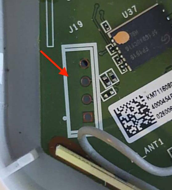
One of the first steps in gaining root access to an IoT device is to identify possible entry points, such as a UART connection. In the case of our exercise, we performed this ahead of time by locating the UART connection and soldering a 2.54 mm header onto the board. This helped streamline the exercise, so attendees could complete it in a reasonable timeframe. However, the typical method to do this is to examine the device’s circuit board looking for an empty header, as in the example shown in Figure 1:

Hands-On IoT Hacking: Rapid7 at DefCon IoT Village, Part 1
Figure 1: Common 4 port 2.54mm header

This example shows 4 port headers. Although 4 port headers are common for UART, it is not always the rule. UART connections can be included in larger port headers or may not even have an exposed header. So, when you find a header that you believe to be UART, you’ll need to validate it.

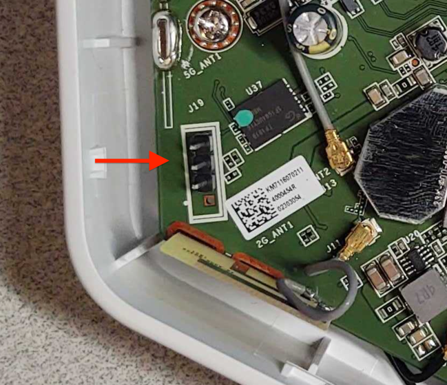
To do this, we first recommend soldering male pins into the exposed socket. This will allow easier connectivity of test equipment. An example of this is shown in Figure 2:

Hands-On IoT Hacking: Rapid7 at DefCon IoT Village, Part 1
Figure 2: Soldered 2.54mm header

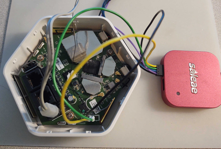
Once you’ve installed a header, I recommend using a logic analyzer to examine the connection for UART data. There are many different logic analyzers available on the market, which range in value from $12 or $15 to hundreds of dollars. In my case, I prefer using a Saleae logic analyzer.

The next step is to identify if any of the header pins are ground. To do this, first make sure the device is powered off. Then, you can use a multimeter set on continuity check and attach the ground lead “Black” to one of the metal shields covering various components on the circuit board, or one of the screws used to hold the circuit board in the cases — both often are found to be electrical ground.

Next, touch each pin in the header with the positive lead “Red” until the multimeter makes a ringing noise. This will indicate which pin is electrically ground. Once you’ve identified ground, you can attach the Logic Analyzer ground to that header pin and then connect the logic channel leads to the remaining pins, as shown in Figure 3:

Hands-On IoT Hacking: Rapid7 at DefCon IoT Village, Part 1
Figure 3: Logic Analyzer hooked up

Once hooked up, make sure the appropriate analyzer software is installed and running. In my case, I used Saleae’s Logic2. You can then power on the device and capture data on this header to analyze and identify:

  • Whether or not this header is UART
  • What the baud rate is
  • Which pin is transmit
  • Which pin is receive

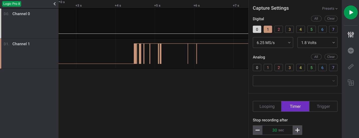
As shown in the capture example in Figure 4, I captured 30 seconds of data during power-up of the device for channel 0 and 1. Here, we can see that data is shown on pin 1, which in this case indicates that channel 1, if determined to be UART, is most likely connected to the transmit pin. Since we are not sending any data to the device, channel 0 should show nothing, indicating it is most likely the receive pin.

Hands-On IoT Hacking: Rapid7 at DefCon IoT Village, Part 1
Figure 4: Logic-2 Capture 30 seconds

The next step is to make a final determination as to whether this is a UART header? If so, what is the baud rate?

We’ll cover this and the subsequent steps in our next post. Check back next week for more!

NEVER MISS A BLOG

Get the latest stories, expertise, and news about security today.

Security updates for Thursday

Post Syndicated from original https://lwn.net/Articles/873601/rss

Security updates have been issued by Debian (python-babel, squashfs-tools, and uwsgi), Fedora (gfbgraph and rust-coreos-installer), Mageia (aom, libslirp, redis, and vim), openSUSE (fetchmail, go1.16, go1.17, mbedtls, ncurses, python, squid, and ssh-audit), Red Hat (java-1.8.0-openjdk and java-11-openjdk), Scientific Linux (java-1.8.0-openjdk and java-11-openjdk), SUSE (fetchmail, git, go1.16, go1.17, ncurses, postgresql10, python, python36, and squid), and Ubuntu (linux, linux-aws, linux-aws-hwe, linux-azure, linux-azure-4.15, linux-dell300x, linux-gcp, linux-gcp-4.15, linux-hwe, linux-kvm, linux-raspi2, linux-snapdragon, linux, linux-bluefield, linux-gcp-5.4, linux-hwe-5.4, linux-kvm, linux-oem-5.10, and linux-oem-5.13).

Creating AWS Serverless batch processing architectures

Post Syndicated from James Beswick original https://aws.amazon.com/blogs/compute/creating-aws-serverless-batch-processing-architectures/

This post is written by Reagan Rosario, AWS Solutions Architect and Mark Curtis, Solutions Architect, WWPS.

Batch processes are foundational to many organizations and can help process large amounts of information in an efficient and automated way. Use cases include file intake processes, queue-based processing, and transactional jobs, in addition to heavy data processing jobs.

This post explains a serverless solution for batch processing to implement a file intake process. This example uses AWS Step Functions for orchestration, AWS Lambda functions for on-demand instance compute, Amazon S3 for storing the data, and Amazon SES for sending emails.

Overview

This post’s example takes a common use-case of a business’s need to process data uploaded as a file. The test file has various data fields such as item ID, order date, order location. The data must be validated, processed, and enriched with related information such as unit price. Lastly, this enriched data may need to be sent to a third-party system.

Step Functions allows you to coordinate multiple AWS services in fully managed workflows to build and update applications quickly. You can also create larger workflows out of smaller workflows by using nesting. This post’s architecture creates a smaller and modular Chunk processor workflow, which is better for processing smaller files.

As the file size increases, the size of the payload passed between states increases. Executions that pass large payloads of data between states can be stopped if they exceed the maximum payload size of 262,144 bytes.

To process large files and to make the workflow modular, I split the processing between two workflows. One workflow is responsible for splitting up a larger file into chunks. A second nested workflow is responsible for processing records in individual chunk files. This separation of high-level workflow steps from low-level workflow steps also allows for easier monitoring and debugging.

Splitting the files in multiple chunks can also improve performance by processing each chunk in parallel. You can further improve the performance by using dynamic parallelism via the map state for each chunk.

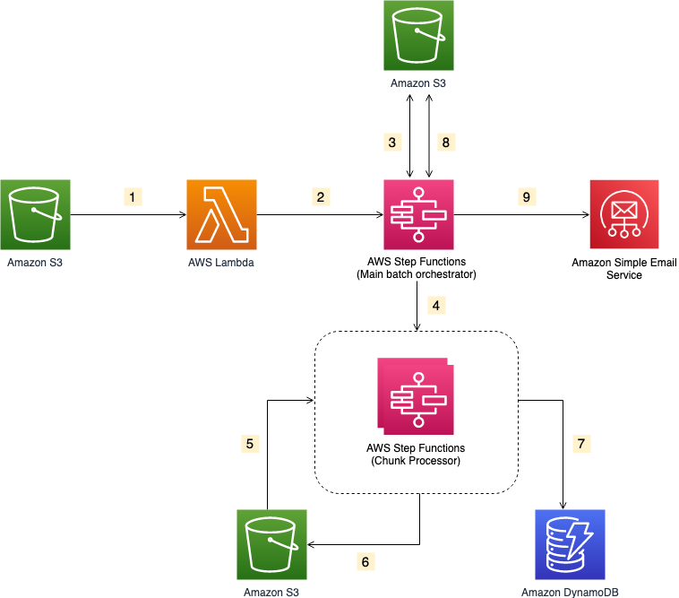
Solution architecture

  1. The file upload to an S3 bucket triggers the S3 event notification. It invokes the Lambda function asynchronously with an event that contains details about the object.
  2. Lambda function calls the Main batch orchestrator workflow to start the processing of the file.
  3. Main batch orchestrator workflow reads the input file and splits it into multiple chunks and stores them in an S3 bucket.
  4. Main batch orchestrator then invokes the Chunk Processor workflow for each split file chunk.
  5. Each Chunk processor workflow execution reads and processes a single split chunk file.
  6. Chunk processor workflow writes the processed chunk file back to the S3 bucket.
  7. Chunk processor workflow writes the details about any validation errors in an Amazon DynamoDB table.
  8. Main batch orchestrator workflow then merges all the processed chunk files and saves it to an S3 bucket.
  9. Main batch orchestrator workflow then emails the consolidated files to the intended recipients using Amazon Simple Email Service.

Step Functions workflow

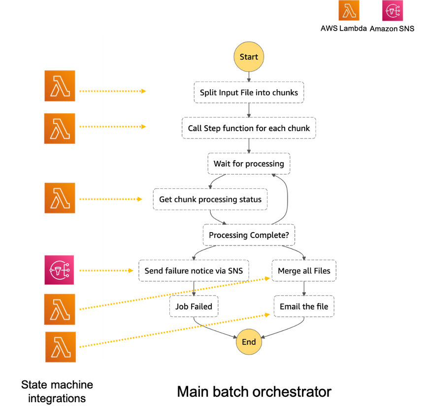
  1. The Main batch orchestrator workflow orchestrates the processing of the file.
    1. The first task state Split Input File into chunks calls a Lambda function. It splits the main file into multiple chunks based on the number of records and stores each chunk into an S3 bucket.
    2. The next task state Call Step Functions for each chunk invokes a Lambda function. It triggers a workflow for each chunk of the file. It passes information such as the name of bucket and the key where the chunk file to be processed is present.
    3. Then we wait for all the child workflow executions to complete.
    4. Once all the child workflows are processed successfully, the next task state is Merge all Files. This combines all the processed chunks into a single file and then stores the file back to the S3 bucket.
    5. The next task state Email the file takes the output file. It generates an S3 presigned URL for the file and sends an email with the S3 presigned URL.Chunk processor workflow
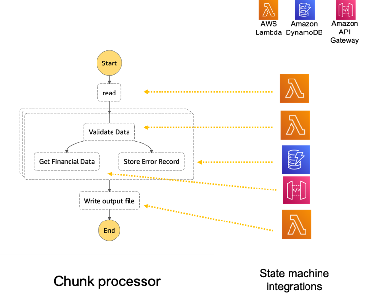
  2. The Chunk processor workflow is responsible for processing each row from the chunk file that was passed.
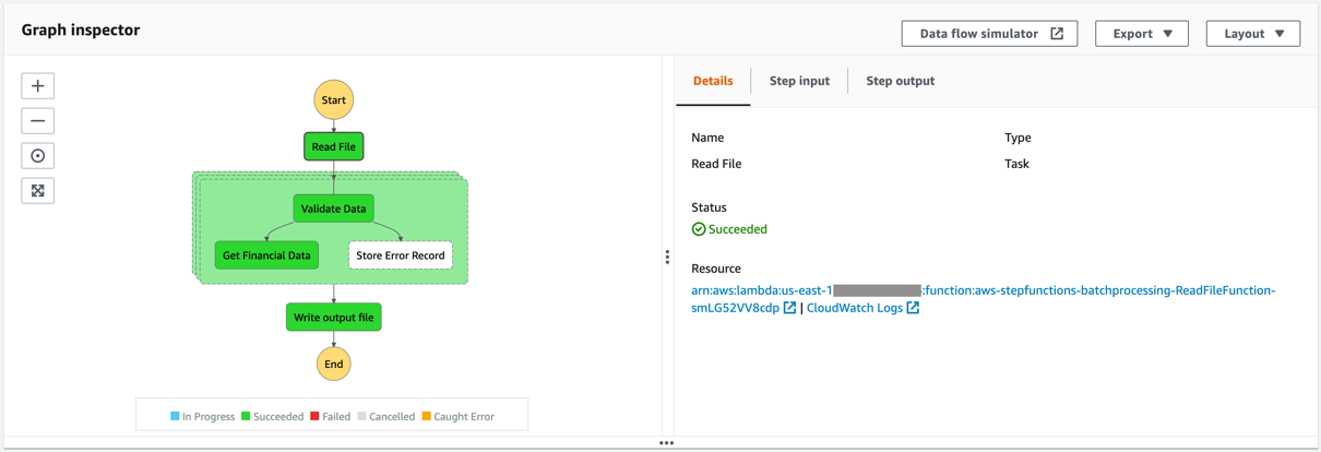
    1. The first task state Read reads the chunked file from S3 and converts it to an array of JSON objects. Each JSON object represents a row in the chunk file.
    2. The next state is a map state called Process messages (not shown in the preceding visual workflow). It runs a set of steps for each element of an input array. The input to the map state is an array of JSON objects passed by the previous task.
    3. Within the map state, Validate Data is the first state. It invokes a Lambda function that validates each JSON object using the rules that you have created. Records that fail validation are stored in an Amazon DynamoDB table.
    4. The next state Get Financial Data invokes Amazon API Gateway endpoints to enrich the data in the file with data from a DynamoDB table.
    5. When the map state iterations are complete, the Write output file state triggers a task. It calls a Lambda function, which converts the JSON data back to CSV and writes the output object to S3.

Prerequisites

Deploying the application

  1. Clone the repository.
  2. Change to the directory and build the application source:
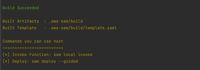
    sam build
    sam build
  3. Package and deploy the application to AWS. When prompted, input the corresponding parameters as shown below:
    sam deploy –guided
    sam deployNote the template parameters:
    • SESSender: The sender email address for the output file email.
    • SESRecipient: The recipient email address for the output file email.
    • SESIdentityName: An email address or domain that Amazon SES users use to send email.
    • InputArchiveFolder: Amazon S3 folder where the input file will be archived after processing.
    • FileChunkSize: Size of each of the chunks, which is split from the input file.
    • FileDelimiter: Delimiter of the CSV file (for example, a comma).
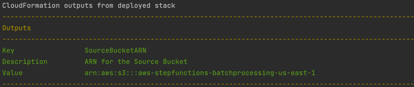
  4. After the stack creation is complete, you see the source bucket created in Outputs.
    Outputs
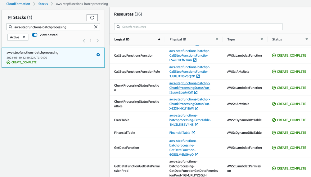
  5. Review the deployed components in the AWS CloudFormation Console.
    CloudFormation console

Testing the solution

  1. Before you can send an email using Amazon SES, you must verify each identity that you’re going to use as a “From”, “Source”, “Sender”, or “Return-Path” address to prove that you own it. Refer Verifying identities in Amazon SES for more information.
  2. Locate the S3 bucket (SourceBucket) in the Resources section of the CloudFormation stack. Choose the physical ID.
    s3 bucket ID
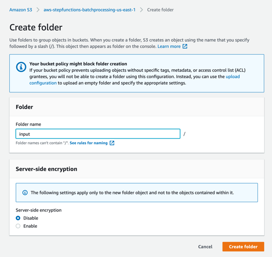
  3. In the S3 console for the SourceBucket, choose Create folder. Name the folder input and choose Create folder.
    Create folder
  4. The S3 event notification on the SourceBucket uses “input” as the prefix and “csv” as the suffix. This triggers the notification Lambda function. This is created as a part of the custom resource in the AWS SAM template.
    Event notification
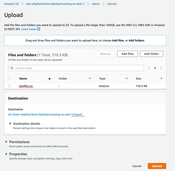
  5. In the S3 console for the SourceBucket, choose the Upload button. Choose Add files and browse to the input file (testfile.csv). Choose Upload.
    Upload dialog
  6. Review the data in the input file testfile.csv.
    Testfile.csv
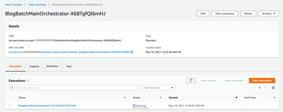
  7. After the object is uploaded, the event notification triggers the Lambda Function. This starts the main orchestrator workflow. In the Step Functions console, you see the workflow is in a running state.
    Step Functions console
  8. Choose an individual state machine to see additional information.
    State machine
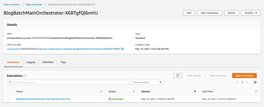
  9. After a few minutes, both BlogBatchMainOrchestrator and BlogBatchProcessChunk workflows have completed all executions. There is one execution for the BlogBatchMainOrchestrator workflow and multiple invocations of the BlogBatchProcessChunk workflow. This is because the BlogBatchMainOrchestrator invokes the BlogBatchProcessChunk for each of the chunked files.
    Workflow #1Workflow #2

Checking the output

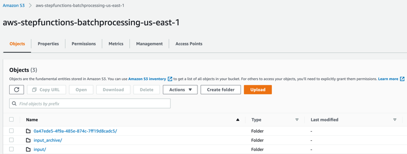
  1. Open the S3 console and verify the folders created after the process has completed.
    S3 folders
    The following subfolders are created after the processing is complete:
    – input_archive – Folder for archival of the input object.
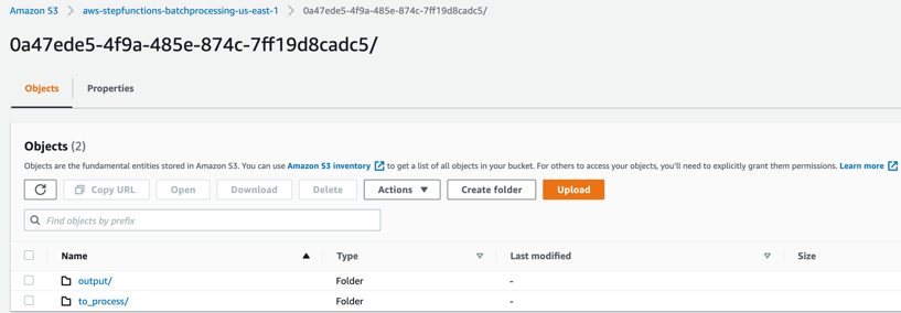
    – 0a47ede5-4f9a-485e-874c-7ff19d8cadc5 – Subfolder with a unique UUID in the name. This is created for storing the objects generated during batch execution.
  2. Select the folder 0a47ede5-4f9a-485e-874c-7ff19d8cadc5.
    Folder contents
    output – This folder contains the completed output objects, some housekeeping files, and processed chunk objects.
    Output folderto_process – This folder contains all the split objects from the original input file.
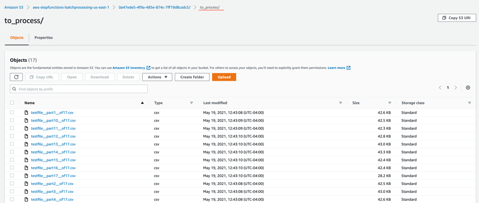
    to_process folder
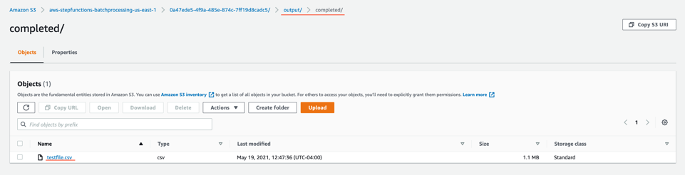
  3. Open the processed object from the output/completed folder.
    Processed object
    Inspect the output object testfile.csv. It is enriched with additional data (columns I through N) from the DynamoDB table fetched through an API call.Output testfile.csv

Viewing a completed workflow

Open the Step Functions console and browse to the BlogBatchMainOrchestrator and BlogBatchProcessChunk state machines. Choose one of the executions of each to locate the Graph Inspector. This shows the execution results for each state.

BlogBatchMainOrchestrator:

BlogBatchMainOrchestrator

BlogBatchProcessChunk:

BlogBatchProcessChunk

Batch performance

For this use case, this is the time taken for the batch to complete, based on the number of input records:

No. of records Time for batch completion
10 k 5 minutes
100 k 7 minutes

The performance of the batch depends on other factors such as the Lambda memory settings and data in the file. Read more about Profiling functions with AWS Lambda Power Tuning.

Conclusion

This blog post shows how to use Step Functions’ features and integrations to orchestrate a batch processing solution. You use two Steps Functions workflows to implement batch processing, with one workflow splitting the original file and a second workflow processing each chunk file.

The overall performance of our batch processing application is improved by splitting the input file into multiple chunks. Each chunk is processed by a separate state machine. Map states further improve the performance and efficiency of workflows by processing individual rows in parallel.

Download the code from this repository to start building a serverless batch processing system.

Additional Resources:

For more serverless learning resources, visit Serverless Land.

Без държава за бъдеще и капачките са бъдеще

Post Syndicated from original https://bivol.bg/%D0%B1%D0%B5%D0%B7-%D0%B4%D1%8A%D1%80%D0%B6%D0%B0%D0%B2%D0%B0-%D0%B7%D0%B0-%D0%B1%D1%8A%D0%B4%D0%B5%D1%89%D0%B5-%D0%B8-%D0%BA%D0%B0%D0%BF%D0%B0%D1%87%D0%BA%D0%B8%D1%82%D0%B5-%D1%81%D0%B0-%D0%B1%D1%8A.html

четвъртък 21 октомври 2021


Сега, на пръв поглед нещата са кристално ясни. Всички знаем, че българското здравеопазване е бездънна каца, в която се набутват едни милиарди, а те изчезват яко дим, без какъвто и…

Problems with Multifactor Authentication

Post Syndicated from Bruce Schneier original https://www.schneier.com/blog/archives/2021/10/problems-with-multifactor-authentication.html

Roger Grimes on why multifactor authentication isn’t a panacea:

The first time I heard of this issue was from a Midwest CEO. His organization had been hit by ransomware to the tune of $10M. Operationally, they were still recovering nearly a year later. And, embarrassingly, it was his most trusted VP who let the attackers in. It turns out that the VP had approved over 10 different push-based messages for logins that he was not involved in. When the VP was asked why he approved logins for logins he was not actually doing, his response was, “They (IT) told me that I needed to click on Approve when the message appeared!”

And there you have it in a nutshell. The VP did not understand the importance (“the WHY”) of why it was so important to ONLY approve logins that they were participating in. Perhaps they were told this. But there is a good chance that IT, when implementinthe new push-based MFA, instructed them as to what they needed to do to successfully log in, but failed to mention what they needed to do when they were not logging in if the same message arrived. Most likely, IT assumed that anyone would naturally understand that it also meant not approving unexpected, unexplained logins. Did the end user get trained as to what to do when an unexpected login arrived? Were they told to click on “Deny” and to contact IT Help Desk to report the active intrusion?

Or was the person told the correct instructions for both approving and denying and it just did not take? We all have busy lives. We all have too much to do. Perhaps the importance of the last part of the instructions just did not sink in. We can think we hear and not really hear. We can hear and still not care.

Hello World’s first-ever special edition is here!

Post Syndicated from Gemma Coleman original https://www.raspberrypi.org/blog/hello-world-big-book-of-computing-pedagogy/

Hello World, our free magazine for computing and digital making educators, has just published its very first special edition: The Big Book of Computing Pedagogy!

“When I started to peruse the draft for The Big Book of Computing Pedagogy, I was simply stunned.”

Monica McGill, founder & CEO of CSEDResearch.org

Cover of The Big Book of Computing Pedagogy.

This special edition focuses on practical approaches to teaching computing in the classroom, and includes some of our favourite pedagogically themed articles from previous issues of Hello World, as well as a few never-seen-before pieces. It is structured around twelve pedagogical principles, first developed by us as part of our work related to the National Centre for Computing Education in England. These twelve principles are based on up-to-date research around the best ways of approaching the teaching and learning of computing.

A girl doing a physical computing project with Raspberry Pi hardware.

Grounded in research and practice

Computing education is still relatively new, and it’s a field that’s constantly changing and adapting. Despite leaving school less than ten years ago, I remember my days in the computer lab being limited to learning about how to add animations on PowerPoints and trying out basic Excel formulas (and yes, there was still the odd mouse with a ball knocking about!).

A tweet praising The Big Book of Computing Pedagogy.
The Big Book of Computing Pedagogy — a big hit with educators!

Computing education research is even younger, and we are proud to be an important part of this growing space. As an organisation, we engage in rigorous original research around computing education and learning for young people, and we share all of our research work through blogs, reports, research seminars, and academic publications. We’re particularly proud to have partnered with the University of Cambridge to establish the Raspberry Pi Computing Education Research Centre. 

12 principles of computing pedagogy: lead with concepts; structure lessons; make concrete; unplug, unpack, repack; work together; read and explore code first; foster program comprehension; model everything; challenge misconceptions; create projects; get hands-on; add variety.
Our special edition of Hello World is organised around twelve pedagogical principles.

The Big Book of Computing Pedagogy represents another way in which we bring research and practice to computing educators in an accessible and engaging way. The book aims to be an educator’s companion to learning about tried and tested approaches to teaching computing.

A tweet praising The Big Book of Computing Pedagogy.
The perfect morning read for computing educators.

It includes articles on techniques for fostering program comprehension, advice for bringing physical computing to your classroom, and introductions to frameworks for structuring your computing lessons. As with all Hello World content, we’re bridging the gap between research and practice by giving you accessible chunks of research, followed by stories of trusty educators who have tried out the approaches in their classroom or educational space.

A tweet praising The Big Book of Computing Pedagogy.
Teachers are jumping for joy at this special edition.

Monica McGill, founder and CEO of CSEDResearch.org, says about Hello World’s latest offering, “When I started to peruse the draft for The Big Book of Computing Pedagogy, I was simply stunned. I found the ready-to-consume content to be solidly based on research evidence and tried-and-true best practices from teachers themselves. This resource provides valuable insights into introducing computing to students via unplugged activities, integrating the Predict–Run–Investigate–Modify–Make (PRIMM) pedagogical model, and introducing physical devices for computing — all written in a way that teachers can adopt and use in their own classrooms.”

We’ve been thrilled to see the reaction of educators to this special edition, with many teachers already using it as a reference guide and for a spot of CPD. Why not join them and download it for free today?

Subscribe now to get each new Hello World — whether regular issue or special edition — straight to your digital inbox, for free! And if you’re based in the UK and do paid or unpaid work in education, you can subscribe for free print issues.

PS Have you listened to our Hello World podcast yet? A new episode has just come out, and it’s great! Listen and subscribe wherever you get your podcasts.

The post Hello World’s first-ever special edition is here! appeared first on Raspberry Pi.

Designing products and services based on Jobs to be Done

Post Syndicated from Grab Tech original https://engineering.grab.com/designing-products-and-services-based-on-jtbd

Introduction

In 2016, Clayton Christensen, a Harvard Business School professor, wrote a book called Competing Against Luck. In his book, he talked about the kind of jobs that exist in our everyday life and how we can uncover hidden jobs through the act of non-consumption. Non-consumption is the inability for a consumer to fulfil an important Job to be Done (JTBD).

JTBD is a framework; it is a different way of looking at consumer goals and is based on the notion that people buy products and services to get a job done. In this article, we will walk through what the JTBD framework is, look at an example of a popular JTBD, and look at how we use the JTBD framework in one of Grab’s services.

JTBD framework

In his book, Clayton Christensen gives the example of the milkshake, as a JTBD example. In the mid-90s, a fast food chain was trying to understand how to improve the milkshakes they were selling and how they could sell more milkshakes. To sell more, they needed to improve the product. To understand the job of the milkshake, they interviewed their customers. They asked their customers why they were buying the milkshakes, and what progress the milkshake would help them make.

Job 1: To fill their stomachs

One of the key insights was the first job, the customers wanted something that could fill their stomachs during their early morning commute to the office. Usually, these car drives would take one to two hours, so they needed something to keep them awake and to keep themselves full.

In this scenario, the competition could be a banana, but think about the properties of a banana. A banana could fill your stomach but your hands get dirty and sticky after peeling it. Bananas cannot do a good job here. Another competitor could be a Snickers bar, but it is rather unhealthy, and depending on how many bites you take, you could finish it in one minute.

By understanding the job the milkshake was performing, the restaurant now had a specific way of improving the product. The milkshake could be made milkier so it takes time to drink through a straw. The customer can then enjoy the milkshake throughout the journey; the milkshake is optimised for the job.

Search data flow
Milkshake

Job 2: To make children happy

As part of the study, they also interviewed parents who came to buy milkshakes in the afternoon, around 3:00 PM. They found out that the parents were buying the milkshakes to make their children happy.

By knowing this, they were able to optimise the job by offering a smaller version of the milkshake which came in different flavours like strawberry and chocolate. From this milkshake example, we learn that multiple jobs can exist for one product. From that, we can make changes to a product to meet those different jobs.

JTBD at GrabFood

A team at GrabFood wanted to prioritise which features or products to build, and performed a prioritisation exercise. However, there was a lack of fundamental understanding of why our consumers were using GrabFood or any other food delivery services. To gain deeper insights on this, we conducted a JTBD study.

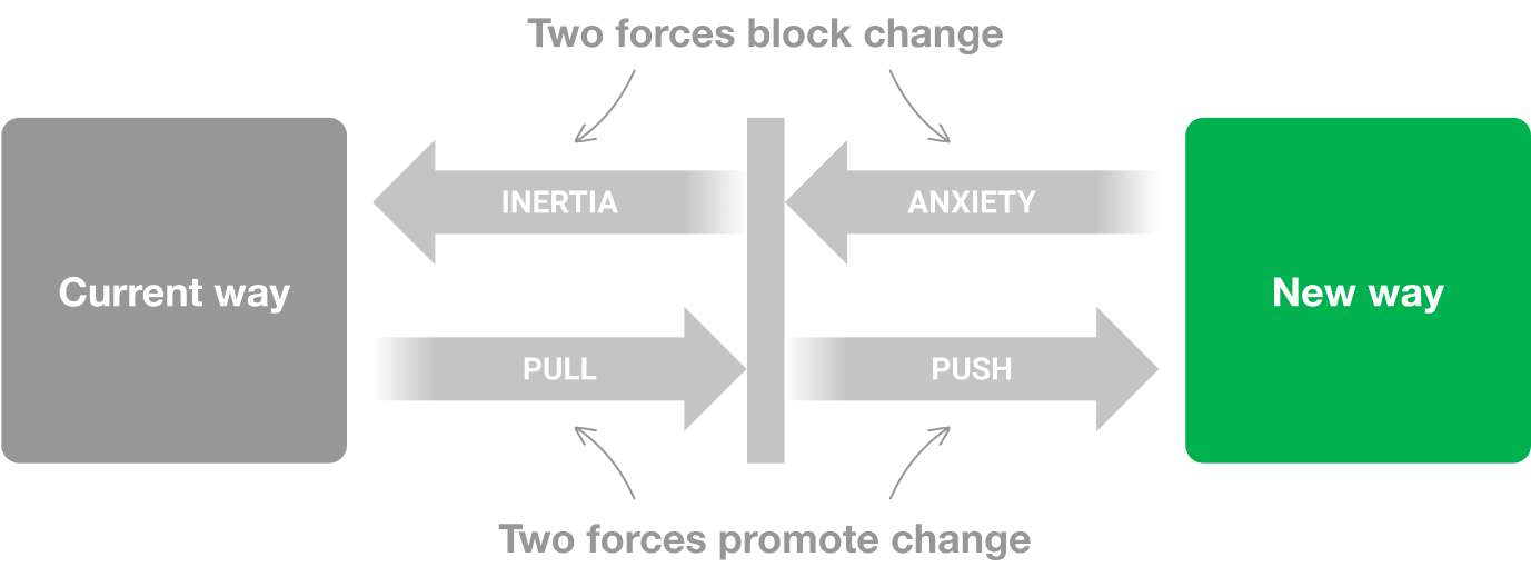
We applied the JTBD framework in our research investigation. We used the force diagram framework to find out what job a consumer wanted to achieve and the corresponding push and pull factors driving the consumer’s decision. A job here is defined as the progress that the consumer is trying to make in a particular context.

Search data flow
Force diagram

There were four key points in the force diagram:

  • What jobs are people using GrabFood for?
  • What did people use prior to GrabFood to get the jobs done?
  • What pushed them to seek a new solution? What is attractive about this new solution?
  • What are the things that will make them go back to the old product? What are the anxieties of the new product?

By applying this framework, we progressively asked these questions in our interview sessions:

  • Can you remind us of the last time you used GrabFood? — This was to uncover the situation or the circumstances.
  • Why did you order this food? — This was to get down to the core of the need.
  • Can you tell us, before GrabFood, what did you use to get the same job done?

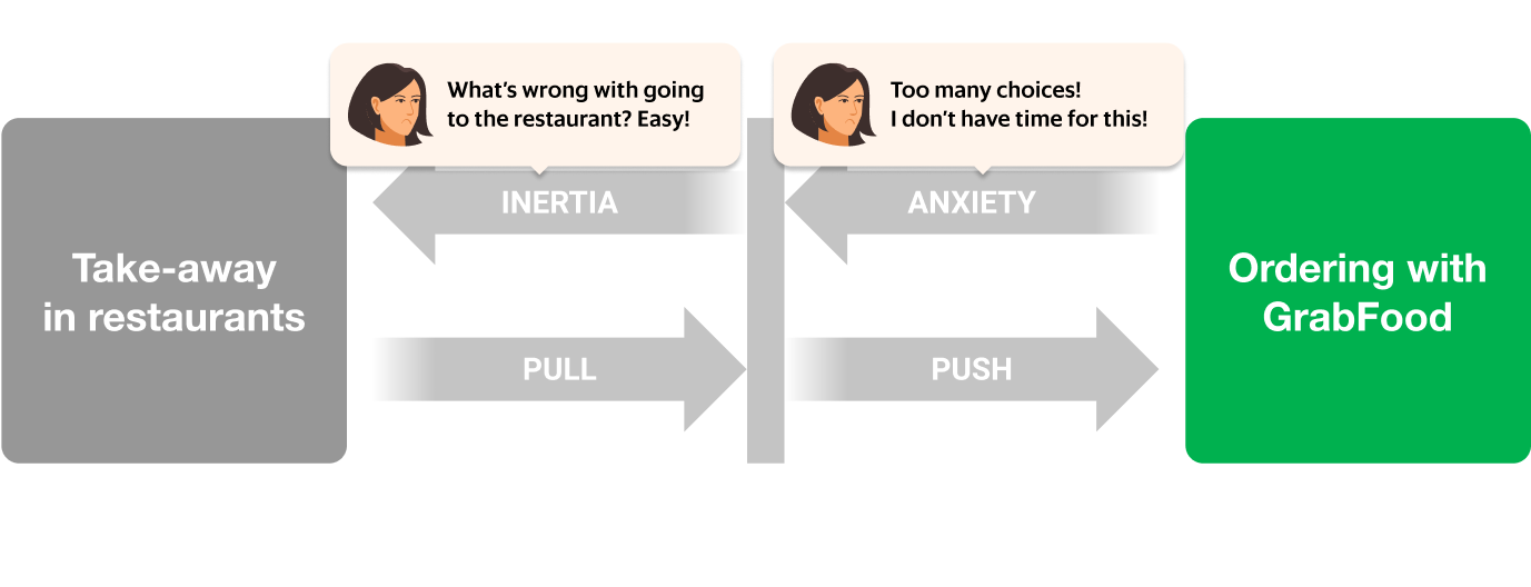
From the interview sessions, we were able to uncover a number of JTBDs, one example was working parents buying food for their families. Before GrabFood, most of them were buying from food vendors directly, but that is a time consuming activity and it adds additional friction to an already busy day. This led them in search of a new solution and GrabFood provided that solution.

Let’s look at this JTBD in more depth. One anxiety that parents had when ordering GrabFood was the sheer number of choices they had to make in order to check out their order:

Search data flow
Force diagram – inertia, anxiety

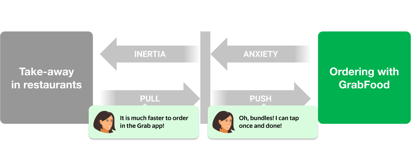
There was already a solution for this problem: bundles! Food bundles is a well-known concept from the food and beverage industry; items that complement each other are bundled together for a more efficient checkout experience.

Search data flow
Force diagram – pull, push

However, not all GrabFood merchants created bundles to solve this problem for their consumers. This was an untapped opportunity for the merchants to solve a critical problem for their consumers. Eureka! We knew that we needed to help merchants create bundles in an efficient way to solve for the consumer’s JTBD.

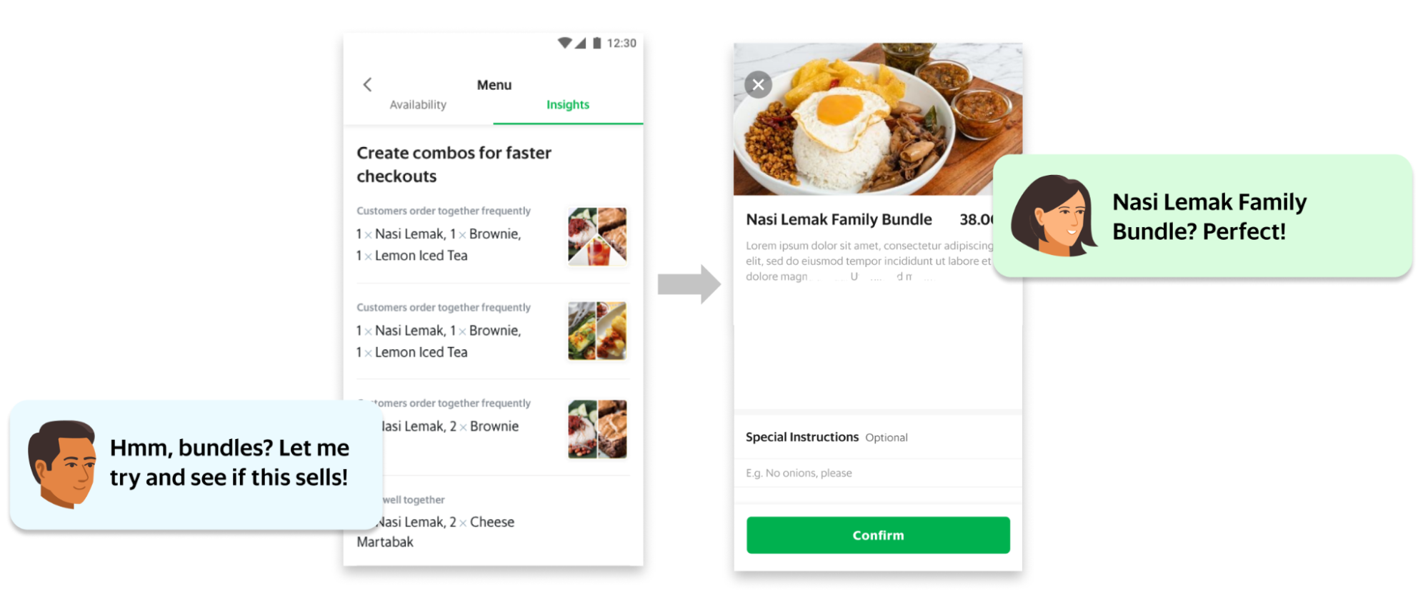
We decided to add a functionality to the GrabMerchant app that allowed merchants to create bundles. We built an algorithm that matched complementary items and automatically suggested these bundles to merchants. The merchant only had to tap a button to create a bundle instantly.

Search data flow
Bundle

The feature was released and thousands of restaurants started adding bundles to their menu. Our JTBD analysis proved to be correct: food and beverage entrepreneurs were now equipped with an essential tool to drive growth and we removed an obstacle for parents to choose GrabFood to solve for their JTBD.

Conclusion

At Grab, we understand the importance of research. We educate designers and other non-researcher employees to conduct research studies. We also encourage the sharing of research findings, and we ensure that research insights are consumable. By using the JTBD framework and asking questions specifically to understand the job of our consumers and partners, we are able to gain fundamental understanding of why our consumers are using our products and services. This helps us improve our products and services, and optimise it for the jobs that need to be done throughout Southeast Asia.

This article was written based on an episode of the Grab Design Podcast – a conversation with Grab Lead Researcher Soon Hau Chua. Want to listen to the Grab Design Podcast? Join the team, we’re hiring!


Special thanks to Amira Khazali and Irene from Tech Learning.


Join us

Grab is a leading superapp in Southeast Asia, providing everyday services that matter to consumers. More than just a ride-hailing and food delivery app, Grab offers a wide range of on-demand services in the region, including mobility, food, package and grocery delivery services, mobile payments, and financial services across over 400 cities in eight countries.

Powered by technology and driven by heart, our mission is to drive Southeast Asia forward by creating economic empowerment for everyone. If this mission speaks to you, join our team today!

Making the Web safer and more secure for everyone

Post Syndicated from Let's Encrypt original https://letsencrypt.org/2021/10/21/celebrating-encryption-globally.html

The Internet Society has supported our work toward a 100% encrypted Web since before we’d even issued our first certificate. Their commitment to helping us execute our vision has been a substantial help over the years. Today, I’m excited to invite Christine Runnegar, Senior Director at The Internet Society and member of ISRG’s Board of Directors, to share her thoughts.

-Josh Aas, Executive Director, ISRG & Let’s Encrypt

Today, across the world, communities, organizations, and individuals are celebrating Global Encryption Day. Organized by the Global Encryption Coalition (GEC), it’s a day to take stock of the crucial role that encryption plays in securing our communications on the Internet.

The Internet Society is a GEC Steering Committee member because access to encryption is a key tool for us to realize our mission of keeping the Internet a force for good. That’s why the Internet Society is also a proud financial sponsor of Internet Security Research Group (ISRG), which founded and operates Let’s Encrypt. Let’s Encrypt provides digital certificates to more than 260 million websites, making a more secure and privacy-respecting Web for users all over the world. In just five years, the percentage of Web pages loaded over HTTPS has risen from under 50% to more than 85% and climbing, principally because of the community that has coalesced around the importance of encryption everywhere. Encrypted Web traffic protects the confidentiality and integrity of information users share with, or learn from, websites. It makes us all safer online.

Let’s Encrypt is a great success story, and an outstanding example of how supporting public interest infrastructure, such as a certificate authority operated for the public’s benefit, helps ensure everyone has access to the benefits of encryption.

We depend on contributions from our community of users and supporters in order to provide our services. If your company or organization would like to sponsor Let’s Encrypt please email us at [email protected]. We ask that you make an individual contribution if it is within your means.

[$] Empowering users of GPL software

Post Syndicated from original https://lwn.net/Articles/873415/rss

A new style of GPL-enforcement lawsuit was
filed
on October 19 by Software Freedom Conservancy (SFC)
against television maker Vizio. Unlike previous GPL-enforcement suits, which
have been pursued on behalf of the developers and copyright holders of
GPL-licensed code, this suit has been filed on behalf of owners of the TVs
in question. The idea that owners of devices that contain code under the
GPL have the right to access that code seems clearly embodied in the
license, but it remains to be seen if the courts will decide that those
owners have the legal standing to sue for relief.

Traffic Sequence: Which Product Runs First?

Post Syndicated from Sam Marsh original https://blog.cloudflare.com/traffic-sequence-which-product-runs-first/

Traffic Sequence: Which Product Runs First?

Traffic Sequence: Which Product Runs First?

“Which came first, the chicken or the egg?” It’s one of life’s great questions. There are hundreds of articles published which conclude with eggs predating chickens by millions of years. Unfortunately, Cloudflare users don’t have New Scientist on hand to answer similar questions.

Which runs first, Firewall Rules or Workers? Page Rules or Transform Rules? Whilst not as philosophically challenging, the answers to these questions are key to setting up your Cloudflare zone correctly. Answering them has become increasingly difficult as more and more functionality is added, thanks to our incredible rate of shipping products. What was once a relatively easy to understand traffic flow exploded in complexity with the introduction of products such as Workers, Load Balancing Rules and Transform Rules. And this big bang of product announcements is only accelerating each year.

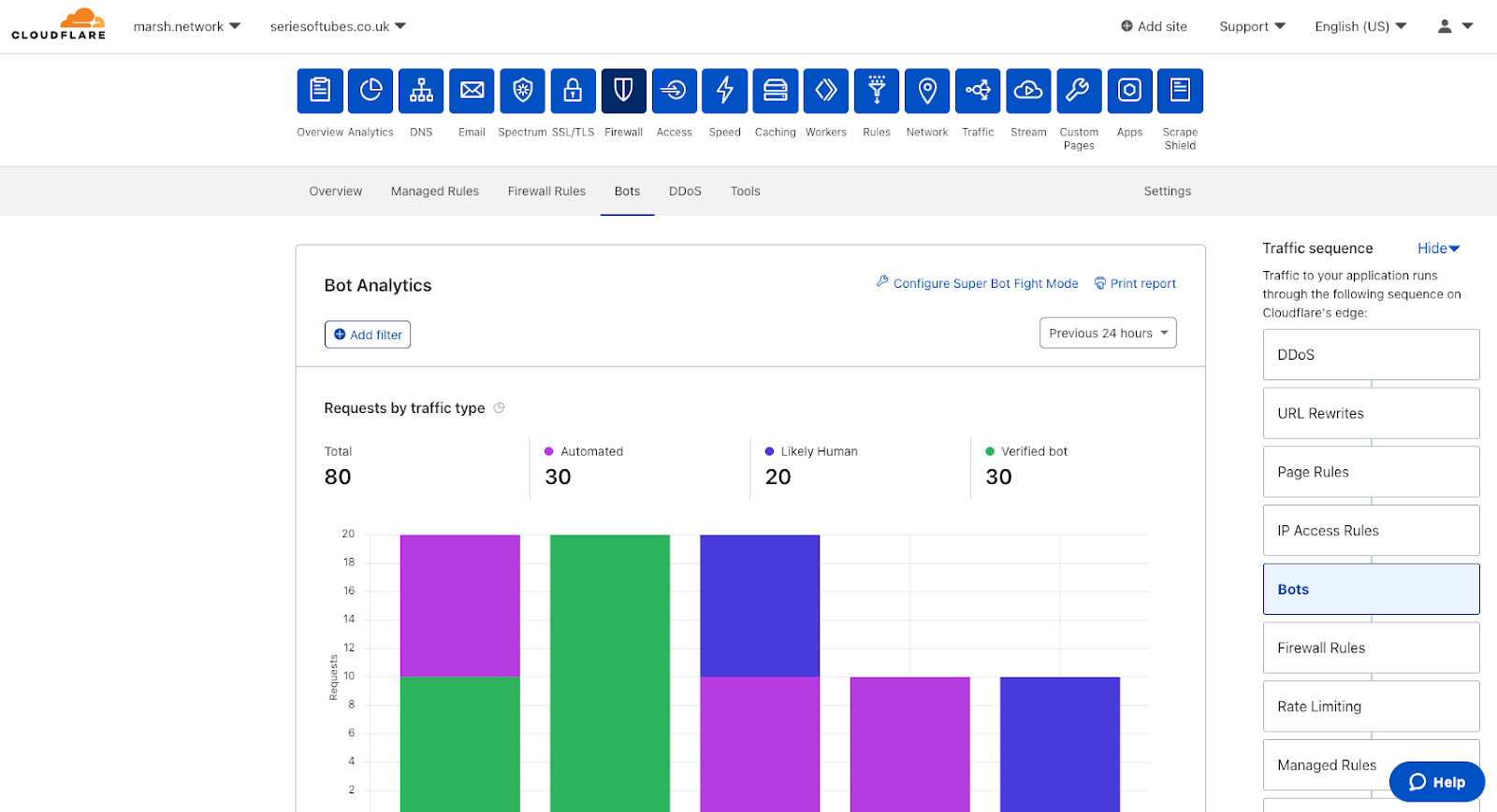
To begin addressing this problem, we developed Traffic Sequence. Traffic Sequence is a simple dashboard illustration which shows a default, high-level overview of how Cloudflare products interact. Think of this as your atlas, rather than your black cab driver’s “Knowledge”. This helps you understand that London is in the south east of the UK, but not that it’s quicker to walk than use the London Underground between Leicester Square and Covent Garden.

Traffic Sequence: Which Product Runs First?

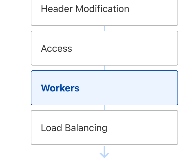
Traffic Sequence is now enabled for all zones by default, appearing on ten product pages within the dashboard. Traffic Sequence highlights in blue the product area you are currently configuring, showing where within the HTTP request lifecycle the specific product sits. This provides context and allows users to understand which products will see the impact of changes here, and which products will not.

Traffic Sequence is designed to make Cloudflare’s edge clearer to our customers, allowing users to understand how products fit together and understand how HTTP requests flow between each.

Dear Cloudflare, which runs first?

Understanding how traffic is routed through Cloudflare has been one of the most common questions from both Cloudflare staff and customers alike.

But why does it matter? Let’s go through a simple example.

Released in April 2021, “Transform Rules” lets users rewrite URLs of HTTP requests as they proxy through their zone — for example, rewriting /login.php to /super/secret/login-page.php, all invisible to the end user.

In this scenario, the administrator also has a Firewall Rule blocking requests to the URI Path /login.php when the visitor is coming from a country other than the United States. What they would see, however, is that visitors from these other countries are still reaching the /login.php page on their servers. Why is this?

This is because URL rewrites happen before Firewall Rules, meaning the Firewall Rules product won’t see a URI Path of /login.php. Instead it will see HTTP requests with the rewritten URI path of /super/secret/login-page.php. Thus, when Firewall Rules evaluates the customers rule it checks:

  1. Is this from a country that is not the USA? Yes
  2. AND – Is this request going to a URI Path of /login.php? No.

As both criteria are not evaluated as ‘true’,  the rule does not match and the traffic is allowed on its journey.

This is why it is so important to know how Cloudflare’s products interoperate to get the most out of your plan, and achieve your goals without having to dig through mountains of documentation.

In an alternate timeline, Traffic Sequence is used to highlight that Firewall Rules run after URL rewriting occurs, and therefore see’s the rewritten value in the URI Path. With this information the customer can then configure a Firewall Rule to look for the rewritten value in URI Path and accomplish their desired setup.

From napkin to working prototype

Traffic Sequence was originally borne out of a “back of the napkin” idea during the creation of Transform Rules and URL Normalization, in an attempt to show where these transformations were happening:

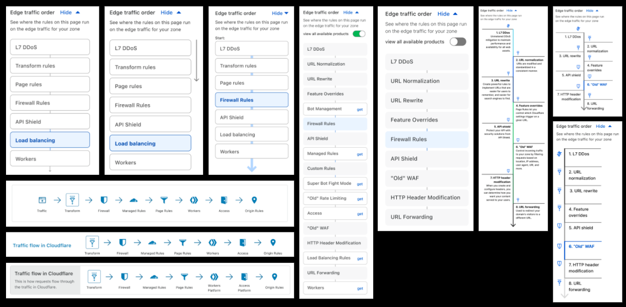
Traffic Sequence: Which Product Runs First?

The idea might have started from a need of our own, but it ended up addressing well known customer and internal problems: whenever we build a new product everyone wants to understand how it fits into the big picture. So we pushed the idea further, proposing it to other teams and soliciting feedback.

This project was a great example of how bringing the right level of fidelity of thinking to the table can be evolved into an opportunity to ship to learn. Something that was initially meant as an explainer diagram for one rule type has become an almost bespoke experience of the dashboard, as it is unique to each customer’s Cloudflare environment, displaying only the products available for use in that zone. We offer many options and routes to products, but we didn’t have a straightforward flow of information that customers can rely on, focusing only on what they have set up and have access to.

As part of the design process, we try to focus on asking lots of questions rather than just finding an answer. Some of the considerations we had were:

  • What if we show customers a product they aren’t using?
  • What if we show customers a product they aren’t entitled to on their plan level?
  • Why aren’t we showing “this product”?
  • Do we have this visualisation on by default?

After gaining internal momentum to flesh out this project, we decided to focus on three areas:

  1. Simplifying a complex ecosystem – what is a useful simplification?
  2. Value that this will add beyond this first application
  3. Opportunity to test out different navigation and mental models.

After all, this is not just a map of our system, but a new way of navigating it entirely.

Positive early internal feedback not only aligned with our goals, but allowed us to iterate on points that needed improvement. We knew that this could be a game-changer for promoting clarity, improving discoverability and saving time with navigation: going for one click instead of three for most items.

Traffic Sequence: Which Product Runs First?

A couple of iterations later, we were ready to put this in the hands of our users for early testing:


Thanks to our incredible community we had a high level of interest in the first week, providing insight into how this feature would be used in the real world, and answering the ultimate question of this experiment: “Does this solve the problem of understanding how Cloudflare handles HTTP requests?”  via our Traffic Sequence survey form:

  • “I didn’t know where my requests were going… until now.”
  • “It’s always been confusing which products/features affect which other products/features.”
  • “It’s really handy to be able to explain the ordering that these are happening in, and I like the deeplink into the relevant area.”

These were all a great reminder that what triggered this work was ingrained in real customer needs.

Other feedback was rapidly incorporated into the prototype; specifically splitting Transform Rules into two separate sections to highlight that URL rewrites and header modifications occur at different parts of the request flow. We also added features which our users deemed important for clarity, such as IP Access Rules.

Traffic Sequence for all

Thanks to the great feedback and participation of all testers, both internal and external, we are now in a position where we are comfortable to take the covers off and make Traffic Sequence available to all users.

Traffic Sequence: Which Product Runs First?

The visualisation can be hidden easily by clicking on the “hide” button, and the display automatically hides to preserve critical whitespace when needed:

Traffic Sequence: Which Product Runs First?

When new products are added, or updates to products occur which modify the traffic order, this diagram will be updated accordingly.

Evolving Traffic Sequence

We know this is a high level, generic overview of how Cloudflare products interact. There is a level of nuance underneath, and a number of products and features not shown in the Traffic Sequence illustration which play an important part in keeping users safe and secure.

In the future we have aspirations to build “the other side of the coin”. Traffic Sequence provides a simple to understand view of how the products work by default at a high level. We also want to create a detailed, almost traceroute-like feature which allows users to see exactly what happens to their traffic — which products it goes via and what happens within those products, and potentially a lot more. Stay tuned!

Try it now

This feature is now enabled by default on all customer zones, and is visible within the dashboard locations outlined above.

Please do try it out and let us know what you think via the Cloudflare Community

Build operational metrics for your enterprise AWS Glue Data Catalog at scale

Post Syndicated from Sachin Thakkar original https://aws.amazon.com/blogs/big-data/build-operational-metrics-for-your-enterprise-aws-glue-data-catalog-at-scale/

Over the last several years, enterprises have accumulated massive amounts of data. Data volumes have increased at an unprecedented rate, exploding from terabytes to petabytes and sometimes exabytes of data. Increasingly, many enterprises are building highly scalable, available, secure, and flexible data lakes on AWS that can handle extremely large datasets. After data lakes are productionized, to measure the efficacy of the data lake and communicate the gaps or accomplishments to the business groups, enterprise data teams need tools to extract operational insights from the data lake. Those insights help answer key questions such as:

  • The last time a table was updated
  • The total table count in each database
  • The projected growth of a given table
  • The most frequently queried table vs. least queried tables

In this post, I walk you through a solution to build an operational metrics dashboard (like the following screenshot) for your enterprise AWS Glue Data Catalog on AWS.

Solution overview

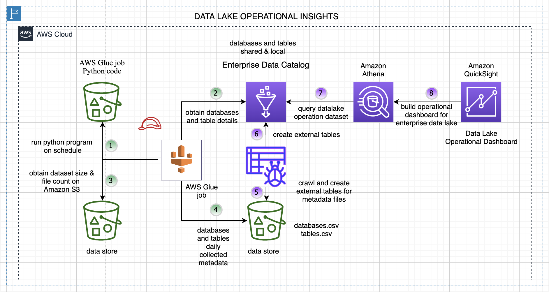
This post shows you how to collect metadata information from your data lake’s AWS Glue Data Catalog resources (databases and tables) and build an operational dashboard on this data.

The following diagram illustrates the overall solution architecture and steps.

The steps are as follows:

  1. A data collector Python program runs on a schedule and collects metadata details about databases and tables from the enterprise Data Catalog.
  2. The following key data attributes are collected for each table and database in your AWS Glue Data Catalog.
Table Data Database Data
TableName DatabaseName
DatabaseName CreateTime
Owner SharedResource
CreateTime SharedResourceOwner
UpdateTime SharedResourceDatabaseName
LastAccessTime Location
TableType Description
Retention
CreatedBy
IsRegisteredWithLakeFormation
Location
SizeInMBOnS3
TotalFilesonS3
  1. The program reads each table’s file location and computes the number of files on Amazon Simple Storage Service (Amazon S3) and the size in MB.
  2. All the data for the tables and databases is stored in an S3 bucket for downstream analysis. The program runs every day and creates new files partitioned by year, month, and day on Amazon S3.
  3. We crawl the data created in Step 4 using an AWS Glue crawler.
  4. The crawler creates an external database and tables for our generated dataset for downstream analysis.
  5. We can query the extracted data with Amazon Athena.
  6. We use Amazon QuickSight to build our operational metrics dashboard and gain insights into our data lake content and usage.

For simplicity, this program crawls and collects data from the Data Catalog for the us-east-1 Region only.

Walkthrough overview

The walkthrough includes the following steps:

  1. Configure your dataset.
  2. Deploy the core solution resources with an AWS CloudFormation template, and set up and trigger the AWS Glue job.
  3. Crawl the metadata dataset and create external tables in the Data Catalog.
  4. Build a view and query the data through Athena.
  5. Set up and import data into QuickSight to create an operational metrics dashboard for the Data Catalog.

Configure your dataset

We use the AWS COVID-19 data lake for analysis. This data lake is comprised of data in a publicly readable S3 bucket.

To make the data from the AWS COVID-19 data lake available in your AWS account, create a CloudFormation stack using the following template. If you’re signed in to your AWS account, the following link fills out most of the stack creation form for you. Make sure to change the Region to us-east-1. For instructions on creating a CloudFormation stack, see Get started.

This template creates a COVID-19 database in your Data Catalog and tables that point to the public AWS COVID-19 data lake. You don’t need to host the data in your account, and you can rely on AWS to refresh the data as datasets are updated through AWS Data Exchange.

For more information about the COVID-19 dataset, see A public data lake for analysis of COVID-19 data.

Your environment may already have existing datasets in the Data Catalog. The program collects the aforementioned attributes for those datasets as well, which can be used for analysis.

Deploy your resources

To make it easier to get started, we created a CloudFormation template that automatically sets up a few key components of the solution:

  • An AWS Glue job (Python program) that is triggered based on a schedule
  • The AWS Identity and Access Management (IAM) role required by the AWS Glue job so the job can collect and store details about databases and tables in the Data Catalog
  • A new S3 bucket for the AWS Glue job to store the data files
  • A new database in the Data Catalog for storing our metrics data tables

The source code for the AWS Glue job and the CloudFormation template are available in the GitHub repo.

You must first download the AWS Glue Python code from GitHub and upload it to an existing S3 bucket. The path of this file needs to be provided when running the CloudFormation stack.

  1. Launch the stack:
  2. Provide values for your parameters as shown in the following screenshot.

After the stack is deployed successfully, you can check the resources created on the stack’s Resources tab.

You can verify and check the AWS Glue job setup and trigger, which is scheduled as per your specified time.

Now that we have verified that the stack is successfully set up, we can run our AWS Glue job manually and collect key attributes for our analysis.

  1. On the AWS Glue console, choose AWS Glue Studio in the navigation pane.
  2. In the AWS Glue Studio Console, click on Jobs and select the DataCollector job and Run the job.

The AWS Glue job collects data and stores it in the S3 bucket created for us through AWS CloudFormation. The job creates separate folders for database and table data, as shown in the following screenshot.

Crawl and set up external tables for the metrics data

Follow these steps to create tables in the database by using AWS Glue crawlers on the data stored on Amazon S3. Note that the database has been created for us using the CloudFormation stack.

  1. On the AWS Glue console, under Databases in the navigation pane, choose Tables.
  2. Choose Add tables.
  3. Choose Add tables using a crawler.
  4. Enter a name for the crawler and choose Next.
  5. For Add crawler, choose Create source type.
  6. Specify the crawler source type by choosing Data stores and choose Next.
  7. In the Add a data store section, for Choose a data store, choose S3.
  8. For Crawl data in, select Specified path.
  9. For Include path, enter the path to the tables folder generated by the AWS Glue job: s3://<data bucket created using CFN>/datalake/tables/.
  10. When asked if you want to create another data store, select No and then choose Next.
  11. On the Choose an IAM Role page, select Choose an Existing IAM Role.
  12. For IAM role, choose the IAM role created through the CloudFormation stack.
  13. Choose Next.
  14. On the Output page, for Database, choose the AWS Glue database you created earlier.
  15. Choose Next.
  16. Review your selections and choose Finish.
  17. Select the crawler you just created and choose Run crawler.

The crawler should take only a few minutes to complete. While it’s running, status messages may appear, informing you that the system is attempting to run the crawler and then is actually running the crawler. You can choose the refresh icon to check on the current status of the crawler.

  1. In the navigation pane, choose Tables.

The table called tables, which was created by the crawler, should be listed.

Query data with Athena

This section demonstrates how to query these tables using Athena. Athena is a serverless, interactive query service that makes it easy to analyze the data in the AWS COVID-19 data lake. Athena supports SQL, a common language that data analysts use for analyzing structured data. To query the data, complete the following steps:

  1. Sign in to the Athena console.
  2. If this is your first time using Athena, you must specify a query result location on Amazon S3.
  3. On the drop-down menu, choose the datalake360db database.
  4. Enter your queries and explore the datasets.

Set up and import data into QuickSight and create an operational metrics dashboard

Set up QuickSight before you import the dataset, and make sure that you have at least 512 MB of SPICE capacity. For more information, see Managing SPICE Capacity.

Before proceeding, make sure your QuickSight account has IAM permissions to access Athena (see Authorizing Connections to Amazon Athena) and Amazon S3.

Let’s first create our datasets.

  1. On the QuickSight console, choose Datasets in the navigation pane.
  2. Choose New dataset.
  3. Choose Athena from the list of data sources.
  4. For Data source name, enter a name.
  5. For Database, choose the database that you set up in the previous step (datalake360db).
  6. For Tables, select databases.
  7. Finish creating your dataset..
  8. Repeat same steps to create a tables dataset.

Now you edit the databases dataset.

  1. From the datasets list, choose the databases dataset.
  2. Choose Edit dataset.
  3. Change the createtime field type from string to date.
  4. Enter the date format as yy/MM/dd HH:mm:ss.
  5. Choose Update.
  6. Similarly, change the tables dataset fields createtime, updatetime, and lastaccessedtime to the date type.
  7. Choose Save and Publish to save the changes to the dataset.

Next, we add calculated fields for the count of databases and tables.

  1. For the tables dataset, choose Add calculation.
  2. Add the calculated field tablesCount as distinct_count({tablename}.
  3. Similarly, add a new calculated field databasesCount as distinct_count({databasename}.

Now let’s create a new analysis.

  1. In the navigation pane, choose Analysis.
  2. Choose the tables dataset.
  3. Choose Create analysis.

Let’s create our first visual for the count of number of databases and tables in our data lake Data Catalog.

  1. Create a new visual and add databasesCount from the fields list.

This provides us with a count of databases in our Data Catalog.

  1. Similarly, add a visual to display the total number of tables using the tablesCount field.

Let’s create second visual for the total number of files on Amazon S3 and total storage size on Amazon S3.

  1. Similar to the previous step, we add a new visual and choose the totalfilesons3 and sizeinmbons3 fields to display Amazon S3-related storage details.

Let’s create another visual to check which are the least used datasets.

  1. Add a visual using the LastAccessTime data element.

Finally, let’s create one more visual to check if databases are shared resources from different accounts.

  1. Select the databases dataset.
  2. We create a table visual type and add databasename, sharedresource, and description fields.

Now you have an idea of what types of visuals are possible using this data. The following screenshot is one example of a finished dashboard.

Clean up

To avoid ongoing charges, delete the CloudFormation stacks and output files in Amazon S3 that you created during deployment. You have to delete the data in the S3 buckets before you can delete the buckets.

Conclusion

In this post, we showed how you can set up an operational metrics dashboard for your Data Catalog. We set up our program to collect key data elements about our tables and databases from the AWS Glue Data Catalog. We then used this dataset to build our operational metrics dashboard and gained insights on our data lake.


About the Authors

Sachin Thakkar is a Senior Solutions Architect at Amazon Web Services, working with a leading Global System Integrator (GSI). He brings over 22 years of experience as an IT Architect and as Technology Consultant for large institutions. His focus area is on Data & Analytics. Sachin provides architectural guidance and supports the GSI partner in building strategic industry solutions on AWS

Configure single sign-on authentication for Amazon Athena with Azure AD integrated to on-premises AD

Post Syndicated from Niraj Kumar original https://aws.amazon.com/blogs/big-data/configure-single-sign-on-authentication-for-amazon-athena-with-azure-ad-integrated-to-on-premises-ad/

Amazon Athena is an interactive query service that makes it easier to analyze data directly in Amazon Simple Storage Service (Amazon S3) using standard SQL. Cloud operation teams can use AWS Identity and Access Management (IAM) federation to centrally manage access to Athena. This simplifies administration by allowing a governing team to control user access to Athena workgroups from a centrally managed Azure AD connected to an on-premise Active Directory. This setup reduces the overhead experience by cloud operation teams when managing IAM users. Athena supports federation with Active Directory Federation Service (ADFS), PingFederate, Okta, and Microsoft Azure Active Directory (Azure AD) federation.

For more information on how to use ADFS with Athena, see Enabling Federated Access to the Athena API. .

This blog post illustrates how to set up AWS IAM federation with Azure AD connected to on-premises AD and configure Athena workgroup- level access for different users. We are going to cover two scenarios:

  1. Azure AD managed users and groups, and on-premises AD.
  2. On-prem Active directory managed users and groups synchronized to Azure AD.

We don’t cover how to setup synchronization between on-premises AD and Azure AD with the help of Azure AD connect. For more information on how to integrate Azure AD with an AWS Managed AD , see Enable Office 365 with AWS Managed Microsoft AD without user password synchronization and how to integrate Azure AD with an on-premises AD , see Microsoft article Custom installation of Azure Active Directory Connect.

Solution overview

This solution helps you configure IAM federation with Azure AD connected to on-premises AD and configure Athena workgroup-level access for users. You can control access to the workgroup by either an on-premises AD group or Azure AD group. The solution consists of four sections:

  1. Set up Azure AD as your identity provider (IdP):
    1. Set up Azure AD as your SAML IdP for an AWS single-account app.
    2. Configure the Azure AD app with delegated permissions.
  2. Set up your IAM IdP and roles:
    1. Set up an IdP trusting Azure AD.
    2. Set up an IAM user with read role permission.
    3. Set up an IAM role and policies for each Athena workgroup.
  3. Set up user access in Azure AD:
    1. Set up automatic IAM role provisioning.
    2. Set up user access to the Athena workgroup role.
  4. Access Athena:
    1. Access Athena using the web-based Microsoft My Apps portal.
    2. Access Athena using SQL Workbench/J a free, DBMS-independent, cross-platform SQL query tool.

The following diagram illustrates the architecture of the solution.

The solution workflow includes the following steps:

  1. The developer workstation connects to Azure AD via a SQL Workbench/j JDBC Athena driver to request a SAML token (two-step OAuth process).
  2. Azure AD sends authentication traffic back to on-premises via an Azure AD pass-through agent or ADFS.
  3. The Azure AD pass-through agent or ADFS connects to on-premises DC and authenticates the user.
  4. The pass-through agent or ADFS sends a success token to Azure AD.
  5. Azure AD constructs a SAML token containing the assigned IAM role and sends it to the client.
  6. The client connects to AWS Security Token Service (AWS STS) and presents the SAML token to assume the Athena role and generates temporary credentials.
  7. AWS STS sends temporary credentials to the client.
  8. The client uses the temporary credentials to connect to Athena.

Prerequisites

You must meet the following requirements prior to configuring the solution:

  • On the Azure AD side, complete the following:
    • Set up the Azure AD Connect server and sync with on-premises AD
    • Set up the Azure AD pass-through or Microsoft ADFS federation between Azure AD and on-premises AD
    • Create three users (user1, user2, user3) and three groups (athena-admin-adgroup, athena-datascience-adgroup, athena-developer-adgroup) for three respective Athena workgroups
  • On the Athena side, create three Athena workgroups: athena-admin-workgroup, athena-datascience-workgroup, athena-developer-workgroup

For more information on using sample Athena workgroups, see A public data lake for analysis of COVID-19 data.

Set up Azure AD

In this section we will cover Azure AD configuration details for Athena in Microsoft Azure subscription. Mainly we will register an app, configure federation, delegate app permission and generate App secret.

Set Azure AD as SAML IdP for an AWS single-account app

To set up Azure AD as your SAML IdP, complete the following steps:

  1. Sign in to the Azure Portal with Azure AD global admin credentials.
  2. Choose Azure Active Directory.
  3. Choose Enterprise applications.
  4. Choose New application.
  5. Search for Amazon in the search bar.
  6. Choose AWS Single-Account Access.
  7. For Name, enter Athena-App.
  8. Choose Create.
  9. In the Getting Started section, under Set up single sign on, choose Get started.
  10. For Select a single sign-on method, choose SAML.
  11. For Basic SAML Configuration, choose Edit.

  12. For Identifier (Entity ID), enter https://signin.aws.amazon.com/saml#1.
  13. Choose Save.
  14. Under SAML Signing Certificate, for Federation Metadata XML, choose Download.

This file is required to configure your IAM IdP in the next section. Save this file on your local machine to use later when configuring IAM on AWS.

Configure your Azure AD app with delegated permissions

To configure your Azure AD app, complete the following steps:

  1. Choose Azure Active Directory.
  2. Choose App registrations and All Applications.
  3. Search for and choose Athena-App.
  4. Note the values for Application (client) ID and Directory (tenant) ID.

You need these values in the JDBC connection when you connect to Athena.

  1. Under API Permissions, choose Add a permission.
  2. Choose Microsoft Graph and Delegated permissions.
  3. For Select permissions, search for user.read.
  4. For User, choose User.Read.
  5. Choose Add permission.
  6. Choose Grant admin consent and Yes.
  7. Choose Authentication and Add a platform.
  8. Choose Mobile and Desktop applications.
  9. Under Custom redirect URIs, enter http://localhost/athena.
  10. Choose Configure.
  11. Choose Certificates & secrets and New client secret.
  12. Enter a description.
  13. For Expires, choose 24 months.
  14. Copy the client secret value to use when configuring the JDBC connection.

Set up the IAM IdP and roles

In this section we will cover IAM configuration in AWS account. Mainly we will create an IAM user, Roles and policies.

Set up an IdP trusting Azure AD

To set up your IdP trusting Azure AD, complete the following steps:

  1. On the IAM console, choose Identity providers in the navigation pane.
  2. Choose Add provider.
  3. For Provider Type, choose SAML.
  4. For Provider Name, enter AzureADAthenaProvider.
  5. For Metadata Document, upload the file downloaded from Azure Portal.
  6. Choose Add provider.

Set up an IAM user with read role permission

To set up your IAM user, complete the following steps:

  1. On the IAM console, choose Users in the navigation pane.
  2. Choose Add user.
  3. For User name, enter ReadRoleUser.
  4. For Access type, select Programmatic access.
  5. Choose Next: Permissions.
  6. For Set permissions, choose Attach existing policies directly.
  7. Choose Create policy.
  8. Select JSON and enter the following policy, which gives read access to enumerate roles in IAM:
    {
        "Version": "2012-10-17",
        "Statement": [
            {
                "Effect": "Allow",
                "Action": [
                    "iam:ListRoles"
                ],
                "Resource": "*"
            }
        ]
    }
    

  9. Choose Next: Tags.
  10. Choose Next: Review.
  11. For Name, enter readrolepolicy.
  12. Choose Create policy.
  13. On the Add User tab, search for and choose the role readrole.
  14. Choose Next: tags.
  15. Choose Next: Review.
  16. Choose Create user.
  17. Download the .csv file containing the access key ID and secret access key.

We use these when configuring Azure AD automatic provisioning.

Set up an IAM role and policies for each Athena workgroup

To set up IAM roles and policies for your Athena workgroups, complete the following steps:

  1. On the IAM console, choose Roles in the navigation pane.
  2. Choose Create role.
  3. For Select type of trusted entity, choose SAML 2.0 federation.
  4. For SAML provider, choose AzureADAthenaProvider.
  5. Choose Allow programmatic and AWS Management Console access.
  6. Under Condition, choose Key.
  7. Select SAML:aud.
  8. For Condition, select StringEquals.
  9. For Value, enter http://localhost/athena.
  10. Choose Next: Permissions.
  11. Choose Create policy.
  12. Choose JSON and enter the following policy (provide the ARN of your workgroup):
{
    "Version": "2012-10-17",
    "Statement": [
        {
            "Effect": "Allow",
            "Action": [
                "athena:ListEngineVersions",
                "athena:ListWorkGroups",
                "athena:ListDataCatalogs",
                "athena:ListDatabases",
                "athena:GetDatabase",
                "athena:ListTableMetadata",
                "athena:GetTableMetadata"
            ],
            "Resource": "*"
        },
        {
            "Effect": "Allow",
            "Action": [
                "athena:BatchGetQueryExecution",
                "athena:GetQueryExecution",
                "athena:ListQueryExecutions",
                "athena:StartQueryExecution",
                "athena:StopQueryExecution",
                "athena:GetQueryResults",
                "athena:GetQueryResultsStream",
                "athena:CreateNamedQuery",
                "athena:GetNamedQuery",
                "athena:BatchGetNamedQuery",
                "athena:ListNamedQueries",
                "athena:DeleteNamedQuery",
                "athena:CreatePreparedStatement",
                "athena:GetPreparedStatement",
                "athena:ListPreparedStatements",
                "athena:UpdatePreparedStatement",
                "athena:DeletePreparedStatement"
            ],
            "Resource": [
                "arn:aws:athena:xxxx:xxxxxx:xxx/xxxx"
            ]
        },
        {
            "Effect": "Allow",
            "Action": [
                "athena:DeleteWorkGroup",
                "athena:UpdateWorkGroup",
                "athena:GetWorkGroup",
                "athena:CreateWorkGroup"
            ],
            "Resource": [
                "arn:aws:athena:xxxx:xxxxxx:xxx/xxxx"
            ]
        },
        {
            "Effect": "Allow",
            "Action": [
                "glue:CreateDatabase",
                "glue:DeleteDatabase",
                "glue:GetDatabase",
                "glue:GetDatabases",
                "glue:UpdateDatabase",
                "glue:CreateTable",
                "glue:DeleteTable",
                "glue:BatchDeleteTable",
                "glue:UpdateTable",
                "glue:GetTable",
                "glue:GetTables",
                "glue:BatchCreatePartition",
                "glue:CreatePartition",
                "glue:DeletePartition",
                "glue:BatchDeletePartition",
                "glue:UpdatePartition",
                "glue:GetPartition",
                "glue:GetPartitions",
                "glue:BatchGetPartition"
            ],
            "Resource": [
                "*"
            ]
        },
        {
            "Effect": "Allow",
            "Action": [
                "s3:GetBucketLocation",
                "s3:GetObject",
                "s3:ListBucket",
                "s3:ListBucketMultipartUploads",
                "s3:ListMultipartUploadParts",
                "s3:AbortMultipartUpload",
                "s3:CreateBucket",
                "s3:PutObject",
                "s3:PutBucketPublicAccessBlock"
            ],
            "Resource": [
                "*"
            ]
        },
        {
            "Effect": "Allow",
            "Action": [
                "s3:GetObject",
                "s3:ListBucket"
            ],
            "Resource": [
                "*"
            ]
        },
        {
            "Effect": "Allow",
            "Action": [
                "s3:ListBucket",
                "s3:GetBucketLocation",
                "s3:ListAllMyBuckets"
            ],
            "Resource": [
                "*"
            ]
        },
        {
            "Effect": "Allow",
            "Action": [
                "sns:ListTopics",
                "sns:GetTopicAttributes"
            ],
            "Resource": [
                "*"
            ]
        },
        {
            "Effect": "Allow",
            "Action": [
                "cloudwatch:PutMetricAlarm",
                "cloudwatch:DescribeAlarms",
                "cloudwatch:DeleteAlarms"
            ],
            "Resource": [
                "*"
            ]
        },
        {
            "Effect": "Allow",
            "Action": [
                "lakeformation:GetDataAccess"
            ],
            "Resource": [
                "*"
            ]
        }
    ]
}

The policy grants full access to Athena workgroup. It’s based on the AWS managed policy AmazonAthenaFullAccess and workgroup example policies.

  1. Choose Next: Tags.
  2. Choose Next: Review.
  3. For Name, enter athenaworkgroup1policy.
  4. Choose Create policy.
  5. On the Create role tab, search for athenaworkgroup1policy and select the policy.
  6. Choose Next: Tags.
  7. Choose Next: Review.
  8. Choose Create role.
  9. For Name, enter athenaworkgroup1role.
  10. Choose Create role.

Set up user access in Azure AD

In this section we will setup Automatic provisioning and assign users to app from Microsoft Azure portal.

Set up automatic IAM role provisioning

To set up automatic IAM role provisioning, complete the following steps:

  1. Sign in to the Azure Portal with Azure AD global admin credentials.
  2. Choose Azure Active Directory.
  3. Choose Enterprise Applications and choose Athena-App.
  4. Choose Provision User Accounts.
  5. In the Provisioning section, choose Get started.
  6. For Provisioning Mode, choose Automatic.
  7. Expand Admin credentials and populate clientsecret and Secret Token with the access key ID and secret access key of ReadRoleUser, respectively.
  8. Choose Test Connection and Save.
  9. Choose Start provisioning.

The initial cycle can take some time to complete, after which the IAM roles are populated in Azure AD.

Set up user access to the Athena workgroup role

To set up user access to the workgroup role, complete the following steps:

  1. Sign in to Azure Portal with Azure AD global admin credentials.
  2. Choose Azure Active Directory.
  3. Choose Enterprise Applications and choose Athena-App.
  4. Choose Assign users and groups and Add user/group.
  5. Under Users and groups, select the group that you want to assign Athena permission to. For this post, we use athena-admin-adgroup; alternatively, you can select user1.
  6. Choose Select.
  7. For Select a role, select the role athenaworkgroup1role.
  8. Choose Select.
  9. Choose Assign.

Access Athena

In this section we will demonstrate how to access Athena from AWS console and developer tool SQL Workbench/J

Access Athena using the web-based Microsoft My Apps portal

To use the Microsoft My Apps portal to access Athena, complete the following steps:

  1. Sign in to Azure Portal with Azure AD global admin credentials.
  2. Choose Azure Active Directory
  3. Choose Enterprise Applications and choose Athena-App.
  4. Choose
  5. Properties.
  6. Copy the value for User access URL.
  7. Open a web browser and enter the URL.

The link redirects you to an Azure login page.

  1. Log in with the on-premises user credentials.

You’re redirected to the AWS Management Console.

Access Athena using SQL Workbench/J

In highly regulated organizations, internal users aren’t allowed to use the console to access Athena. In such cases, you can use SQL Workbench/J, an open-source tool that enables connectivity to Athena using a JDBC driver.

  1. Download the latest Athena JDBC driver (choose the appropriate driver based on your Java version).
  2. Download and install SQL Workbench/J.
  3. Open SQL Workbench/J.
  4. On the File menu, choose Connect Window.
  5. Choose Manage Drivers.
  6. For Name, enter a name for your driver.
  7. Browse to the folder location where you downloaded and unzipped the driver.
  8. Choose OK.

Now that we configured the Athena driver, it’s time to connect to Athena. You need to fill out the connection URL, user name, and password.

Use the following connection string to connect to Athena with a user account without MFA (provide the values collected earlier in the post):

jdbc:awsathena://AwsRegion=xxxx;AwsCredentialsProviderClass=com.simba.athena.iamsupport.plugin.AzureCredentialsProvider;tenant_id=xxxx;client_id=xxxx;Workgroup=xxxx;client_secret=xxxx

To connect using a user account with MFA enabled, use the browser Azure AD Credentials Provider. You need to construct the connection URL and fill out the user name Username and password

Use the following connection string to connect to Athena with a user account that has MFA enabled (provide the values you collected earlier):

jdbc:awsathena://AwsRegion=xxxx;AwsCredentialsProviderClass=com.simba.athena.iamsupport.plugin.BrowserAzureCredentialsProvider;tenant_id=xxxx;client_id=xxxx;Workgroup=xxxx;

Replace text in red with details collected earlier in the article.

When the connection is established, you can run queries against Athena.

Proxy configuration

If you’re connecting to Athena through a proxy server, make sure that the proxy server allows port 444. The result set streaming API uses port 444 on the Athena server for outbound communications. Set the ProxyHost property to the IP address or host name of your proxy server. Set the ProxyPort property to the number of the TCP port that the proxy server uses to listen for client connections. See the following code:

jdbc:awsathena://AwsRegion=xxxx;AwsCredentialsProviderClass=com.simba.athena.iamsupport.plugin.BrowserAzureCredentialsProvider;tenant_id=xxxx;client_id=xxxx;Workgroup=xxxx;ProxyHost=xxxx;ProxyPort=xxxx

Summary

In this post, we configured IAM federation with Azure AD connected to on-premises AD and set up granular access to an Athena workgroup. We also looked at how to access Athena through the console using the Microsoft My Apps web portal and SQL Workbench/J tool. We also discussed how the connection works over a proxy. The same federation infrastructure can also be leveraged for ODBC driver configuration. You can also use the instructions in this post to set up SAML-based Azure IdP to enable federated access to Athena Workgroups.


About the Author

Niraj Kumar is a Principal Technical Account Manager for financial services at AWS, where he helps customers design, architect, build, operate, and support workloads on AWS in a secure and robust manner. He has over 20 years of diverse IT experience in the fields of enterprise architecture, cloud and virtualization, security, IAM, solution architecture, and information systems and technologies. In his free time, he enjoys mentoring, coaching, trekking, watching documentaries with his son, and reading something different every day.

The collective thoughts of the interwebz