Тези дни ми сигнализираха, че е въведено ограничение в свалянето на отворените данни в кадастъра. През януари 2025 писах, че заедно с новата им система са въведени отворени данни включващи всички поземлени имоти, сгради и самостоятелни обекти заедно с анонимизирани данни за собствеността. Скоро след това писах за някои недостатъци на предоставената информация и причината за тях. От тогава тези данни са крайъгълен камък на десетки анализи и визуализации, които съм правил аз и много други. В това число данните за държавните имоти с отпаднала необходимост и имотите на вероизповеданията.
Както писах преди две години обаче свалянето на данните не е лесно. Разделени са на по шест архива с пространствени данни или такива за собственост за всяко село или град в България. Не всички населени места имат всички данни за всички обекти. Някои всъщност нямат никакви използваеми данни, защото просто не са нанесени в кадастъра, а има фиктивен „парцел“ обхващащ цялото село.
Така за да получите всичко за България, трябва да свалите над 23 хилядиархива. Отделно, за да разберете кои населени места какви данни имат и как се казват файловете, трябва да свалите още 5407 индекс файла. За целта направих скрипт, който използвам веднъж в месеца, за да получа последните промени. След това обръща формата на кадастъра (SHP) в по-лесен за използване във визуализации (geojson и csv) и събира всички данни за собствеността в един общ архив. В ZIP индексът е 3.4 Мб. Таблицата със собствеността е около 800 Мб. Очертанията на всички обекти в пространствени данни са 2.2Гб. Държа ги в три ZIP файла. За да ги получа се налага да сваля над 28 хиляди файла с общ размер от 6.5 Гб от кадастъра.
Нови ограничения
Последно свалих данните на 15-ти октомври. Скоро след това разбрах, че е въведено ограничение. Проверих на 21-ви и наистина е така. След известна активност блокират всеки, който се опитва да свали отворените данни. Ограничението е временно, но достатъчно, за да направи още по-труден достъпа от преди.
Попитах ги за причините, какви са измеренията на натоварването и дали е временно докато въведат друго решение. Всъщност, още в началото на 2025-та предупредих, че начинът на публикуване ще им създаде проблеми. Нищо не пречи да пакетират данните в 28 архива за всяка област. Всеки ще е от няколко стотин Мб и ще трябват 28 заявки към сървъра, а не 28 хиляди. Отделно създаването на нов архив при всяка промяна изисква същите ресурси за обновяване на няколко файла в един голям архив.
Когато го предложих тогава един аргумент беше, че при обновяване на данните за едно населено място ще се обнови само архива за него и съответно при желание всеки ще има нужда да сваля само обновените. Това звучи логично, но практиката показва друго. За да се разбере кои файлове са обновени пак трябва да се направят няколко стотин запитвания към индекс файловете и доста по-сложна логика. Т.е. някой трябва да прави програма или скрипт като моя специално за това. Най-вече обаче видяхме, че практически всички общини имат промени в рамките на даден месец и така или иначе повечето информация трябва да се сваля наново.
Казано иначе, чисто технически не пречи да се групират данните в 28 архива и отказът им да го направят е причината за трудностите, с които се аргументират в момента. Отделно, че съдейки по обществената поръчка, ако са получили сървърите, за които са платили, не би трябвало да имат затруднения дори със сегашното положение.
Когато някой бъде блокиран така, на страницата се показва мейл адрес. Очаквам все още отговор на мейла, който писах до него. Междувременно получих отговор на Fb страницата им по същата тема. Надявам се техническите лица да дадат по-смислена информация.
Най-вече се надявам да махнат ограничението и да направят свалянето на отворените данни практично. Както съм казвал много пъти в интервюта и лекции, ключова характеристика на отворените данни е не само, че са в подходящ формат, добре описани и изчерпателни, но и че са свободни за сваляне и използване. Това означава техническа и юридическа възможност и достъпност. Сайтът на министерството – както и твърде много обществени органи – все още има лиценз с „всички права запазени“, което е абсурдно юридически за държавна институция. В случая обаче спъват и техническата достъпност.
Давал съм данните на кадастъра многократно като положителен пример за критични данни, които подпомагат на разследвания, визуализации и инструменти, които нашумяха много в последните две години. Първият случай да ги спомена мисля, че беше е лекцията ми за Ratio. С това просто техническо недомислие обаче тръгват в обратната посока. Това изглежда се явява системен проблем в действията на този кабинет.
Ново заснемане на България
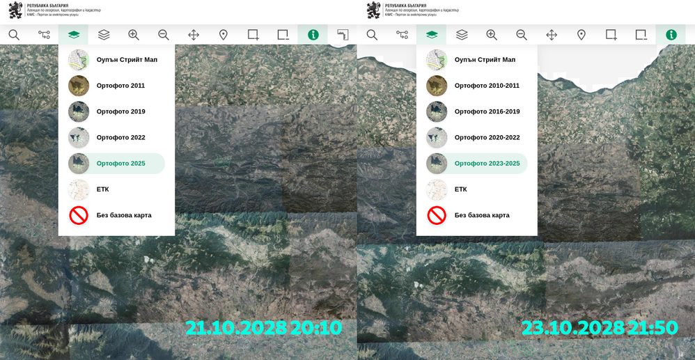
Междувременно МРРБ обявиха, че са добавили нов слой с ортофото заснемане на България. Това е аналогично на добре познатите сателитни снимки на картите на Google, Apple и много други. В случая обаче е поръчано от български институции и се прави независимо от големите доставчици. Обновяването е добре, защото последните данни бяха на четири години. Странното обаче е, че беше представено както иновация и разширяване на възможностите при условие, че съществува като функционалност в различни формати от 15 години.
Разгледах го подробно и забелязах нещо странно. Заснемането беше представено в изказванията като актуално към 2026 г. В самата карта беше маркирано като направено през 2025 г. Разгледах София специално търсейки конкретни строежи, за които знам кога са започнали и на каква фаза са били в последните години. Видях, че на заснемането бул. Филип Кутев не е бил дори завършен. Това значи, че поне южна София е била заснета през лятото на 2023 г. и новите снимки са на поне три години.
После се оказа, че всъщност са имали предвид, че МРРБ са получили данните през март 2026 г., а заснемането е било в периода между 2023 и 2025 г. Това е нормално предвид, че България е голяма и не могат да я заснемат със самолети за няколко месеца или да използват сателитни снимки без облачна покривка за кратък период от време. След коментара ми във Fb забелязах, че са променили заглавията на слоевете с по-точна информация, което приветствам.
Новото заснемане определено е полезно, макар и не актуално и не някаква нова функционалност. Снимките са по-нови от тези на Google Maps, както и 3D заснемането, което използвам във визуализацията на застрояването. Специално за София има публично по-ново заснемане от 2024 г., което е достъпно на iSofMap. Знам, че и други градове в България имат подобни. Така получаваме доста интересна снимка през година от различни източници.
Much of an organization’s most valuable knowledge sits in documents such as contracts, product manuals, research reports, support runbooks, and financial filings. This content is stored in Amazon Simple Storage Service (Amazon S3) as structured data (JSON, NDJSON, and JSON array) and unstructured data (PDF, Word, text, and Markdown). Generative AI applications, Retrieval Augmented Generation (RAG) assistants, and enterprise search experiences are only as good as their access to this content. Yet it’s often the hardest data to make discoverable and searchable. To extract this data, customers must run complex ingestion pipelines with multiple steps:
Running a document parser that extracts text while keeping the layout, reading order, and tables.
Extracting and interpreting the charts, diagrams, and screenshots inside those documents.
Chunking and processing the extracted text through an embedding model and writing the results into a vector index.
Each layer brings its own infrastructure, scaling decisions, and failure modes. The complexity compounds, and many organizations spend weeks to make it work end to end.
Today, we’re excited to announce Amazon OpenSearch intelligent ingestion, a fully managed and serverless ingestion capability in Amazon OpenSearch Serverless (NextGen). You start from your collection, point to your data in Amazon S3, and choose how it should be processed. Intelligent ingestion then handles the rest: it discovers your content from S3, parses the documents, describes the images, chunks the content, generates vector embeddings, and indexes the results. There are no pipelines to configure, no document processing infrastructure to operate, and no capacity to size ahead of time.
With intelligent ingestion, you can:
Go from raw documents to semantic search without manual pipelines. Ingest PDF, Word, and Markdown files, parsed with their layout and tables intact, into indexes ready for semantic and hybrid search.
Make visual content searchable. When documents contain charts, diagrams, screenshots, or photos, a vision-language model writes detailed text descriptions. You can then find information that only appears in images.
Ingest structured data without pipeline code. Load JSON, NDJSON, and CSV data and apply transformations during ingestion, with optional semantic search enrichment.
Choose one-time or continuous ingestion streams. Use Ingestion Jobs for one-time or periodic loads such as migrations and backfills. Use Ingestion Streams to keep your index continuously in sync as new objects arrive in your bucket.
Pay only for active processing. Capacity scales automatically with your workload, and you aren’t charged for idle ingestion capacity.
In this post, we explain how intelligent ingestion works and when to use Ingestion Jobs or Ingestion Streams. We then walk through ingesting a batch of unstructured documents from Amazon S3 and processing their contents into RAG-ready intelligence in Amazon OpenSearch Serverless (NextGen). You can ingest logs and structured data with the same workflow. Load JSON, NDJSON, and JSON array data, such as application logs, audit trails, or product catalogs, from Amazon S3 and apply transformations during ingestion, with optional semantic enrichment. Your RAG knowledge base and your log analytics can share a single ingestion experience.
Solution overview
Intelligent ingestion runs inside Amazon OpenSearch Serverless (NextGen) collections and manages the whole path from your S3 bucket to your index. When you create an Ingestion Job or an Ingestion Stream, you only need to specify two things:
The source – An Amazon S3 bucket and prefix that contain your data.
The destination – The index in your Amazon OpenSearch Serverless (NextGen) collection where the processed data lands.
From there, intelligent ingestion runs the following steps for you.
Data discovery: Intelligent ingestion automatically scans the objects under your S3 prefix. For Ingestion Streams, it detects new objects as they arrive using Amazon Simple Queue Service (Amazon SQS) notifications.
Document parsing: When PDF and Word files are detected, intelligent ingestion automatically parses them into structured content, keeping headings, reading order, and tables.
Image understanding: When it detects images in the PDF and Word files, it generates rich text descriptions so visual content can be indexed alongside the surrounding text.
Chunking and embedding: Intelligent ingestion splits content into chunks sized for retrieval and generates vector embeddings using OpenSearch Automatic Semantic Enrichment.
Indexing: Intelligent ingestion writes the chunks, sparse embeddings, and metadata into your index and scales capacity up and down for the workload, within your predefined OpenSearch Compute Unit (OCU) limits for the collection group.
Ingestion Jobs or Ingestion Streams
Ingestion Jobs
Ingestion Streams
Use when
You have a fixed dataset to load once
Your data keeps arriving or changing
Typical scenarios
Initial loads, migrations, backfills, proofs of concept
Knowledge bases that grow, continuously updated document libraries
Behavior
Ingests all objects under the prefix, then completes
Keeps the index in sync as new objects arrive
Prerequisites
To follow along with this post, you need:
An AWS account with permissions to create and manage Amazon OpenSearch Serverless (NextGen) collections.
An Amazon S3 bucket containing your data.
An AWS Identity and Access Management (IAM) role and the permissions required for intelligent ingestion to read from Amazon S3.
How it works
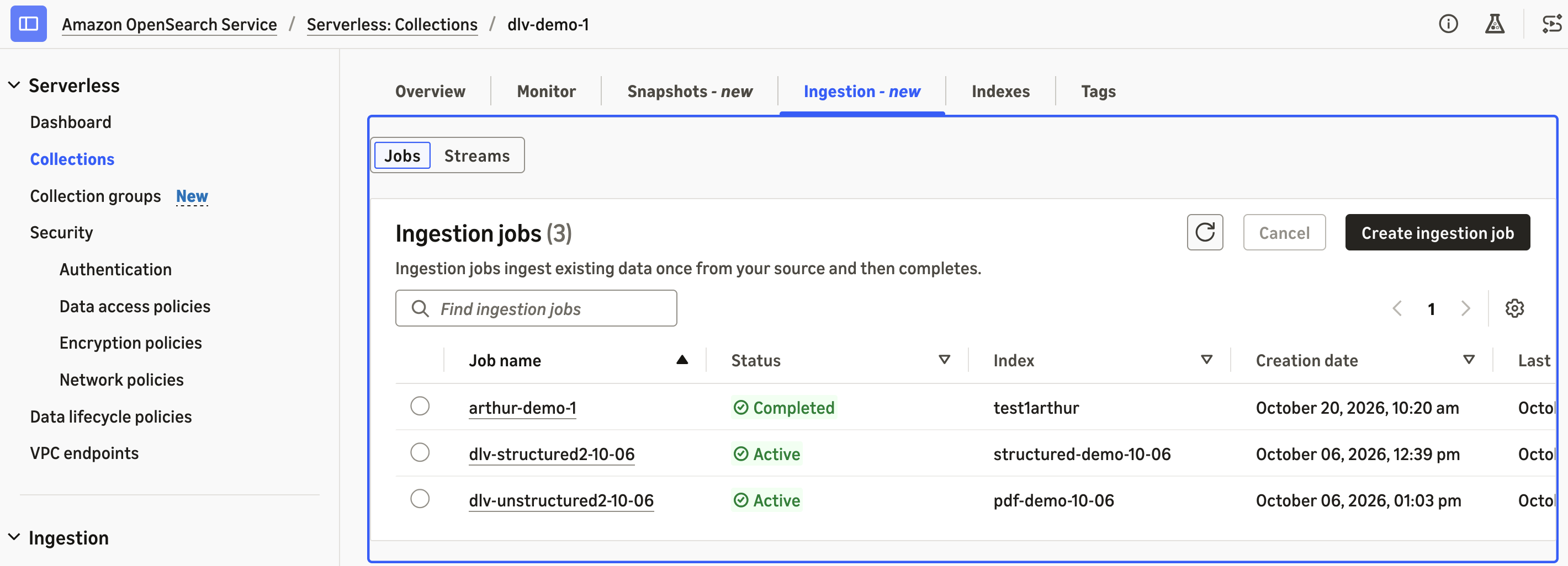
Starting from the AWS Management Console page for Amazon OpenSearch Serverless, you can now see a new Ingestion tab. You can start by choosing Create ingestion job, or review the existing jobs on this tab.
Figure 1: The Ingestion tab on the Amazon OpenSearch Service console
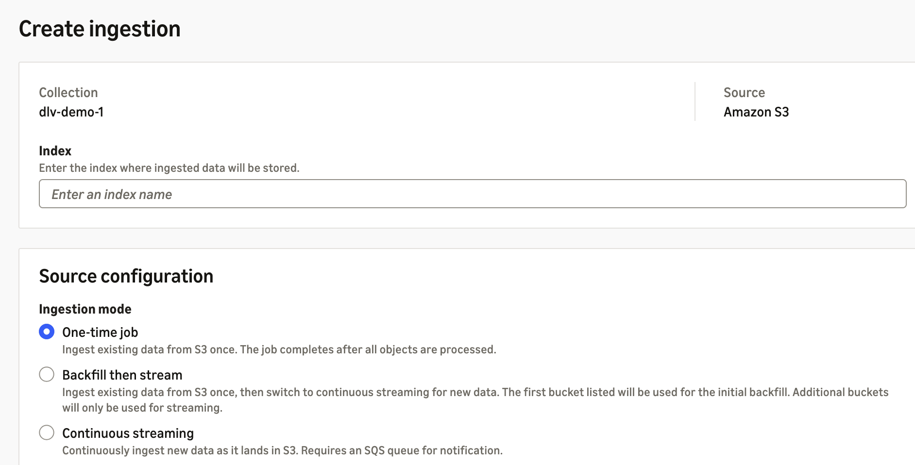
Intelligent ingestion supports three modes for different source configurations. For a static dataset on Amazon S3, select One-time batch to ingest it once, and the ingestion job automatically terminates after completion.
Figure 2: Selecting the One-time batch ingestion mode
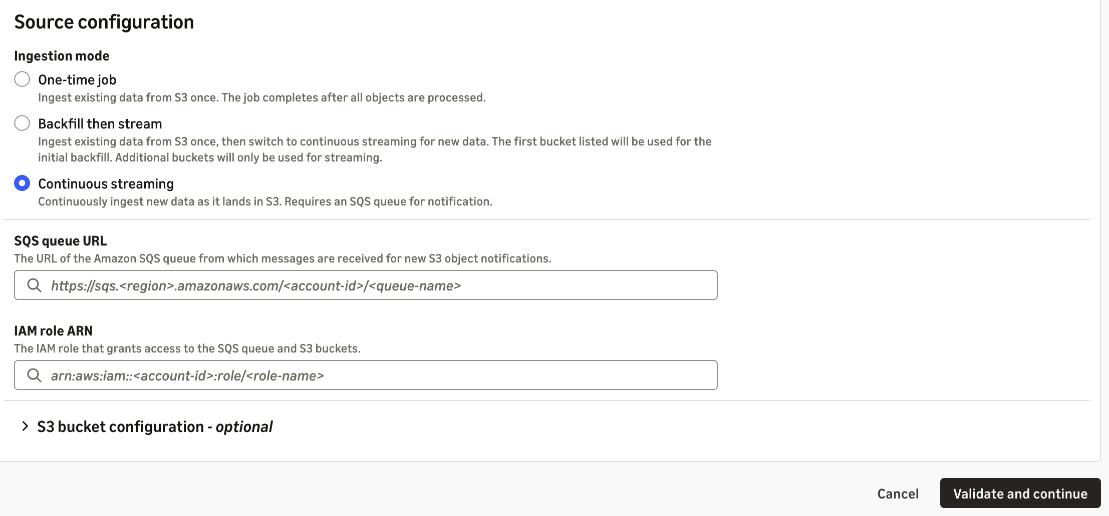
For new S3 buckets that are about to receive new data input, select Continuous streaming to continuously monitor notifications and ingest when new data becomes available. If the S3 bucket already has some data in it, select Batch then stream to ingest the existing data and then switch to continuous streaming mode. For both scenarios, intelligent ingestion relies on your Amazon SQS queue to receive Amazon S3 object notifications, and requires the Amazon Resource Name (ARN) of an IAM role to assume and operate it for data ingestion.
Figure 3: Configuring continuous streaming with an Amazon SQS queue and IAM role
Backfill then stream works as a combination of the other two modes. You can specify one bucket for the initial backfill and additional buckets for streaming new data.
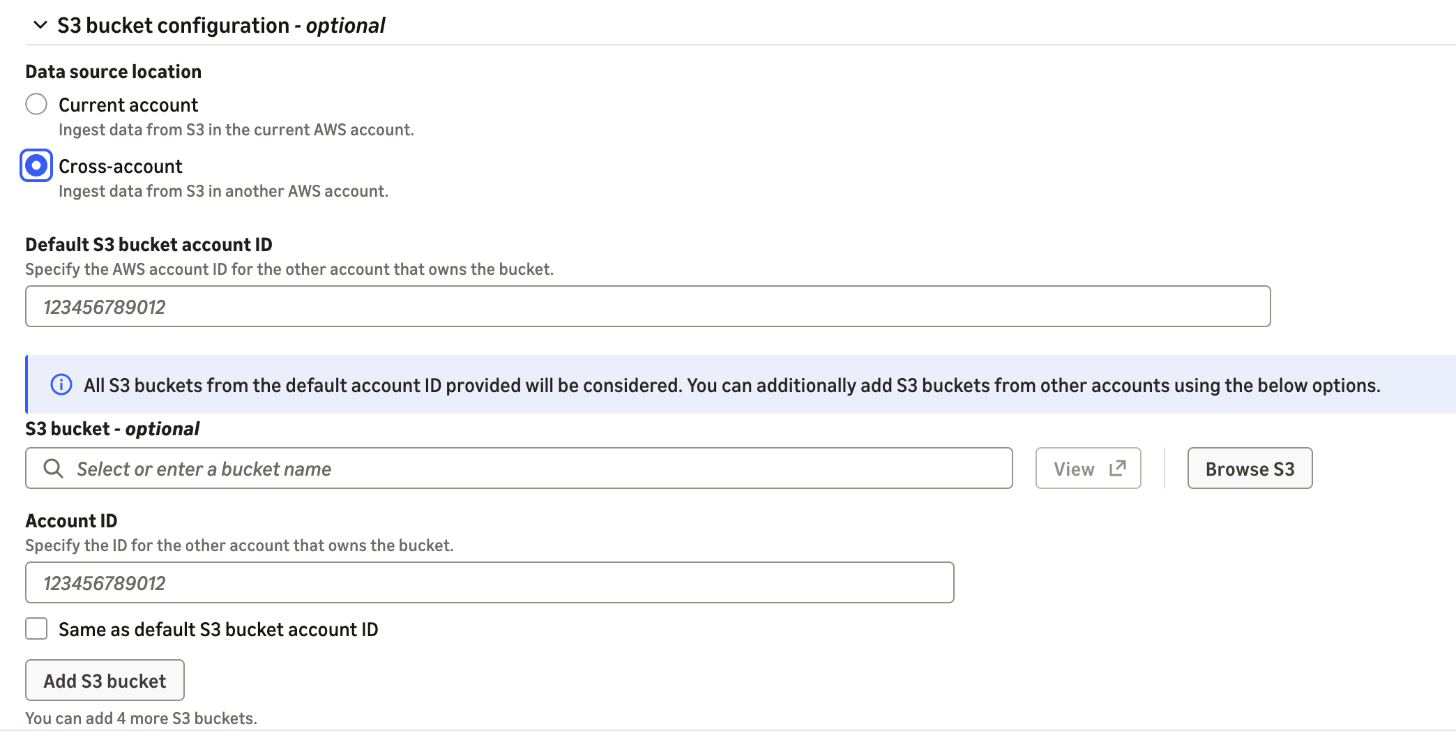
The intelligent ingestion feature works automatically with S3 buckets within the same AWS account. You can browse for the S3 bucket within this page, and optionally define a prefix to specify which folders or files within the bucket should be ingested. Intelligent ingestion also works with S3 buckets in a different AWS account. For cross-account, you need to provide the other AWS account ID, along with the Amazon S3 bucket, IAM role ARN, and optionally Amazon SQS in that account to access both resources.
Figure 4: Selecting an Amazon S3 bucket and optional cross-account access
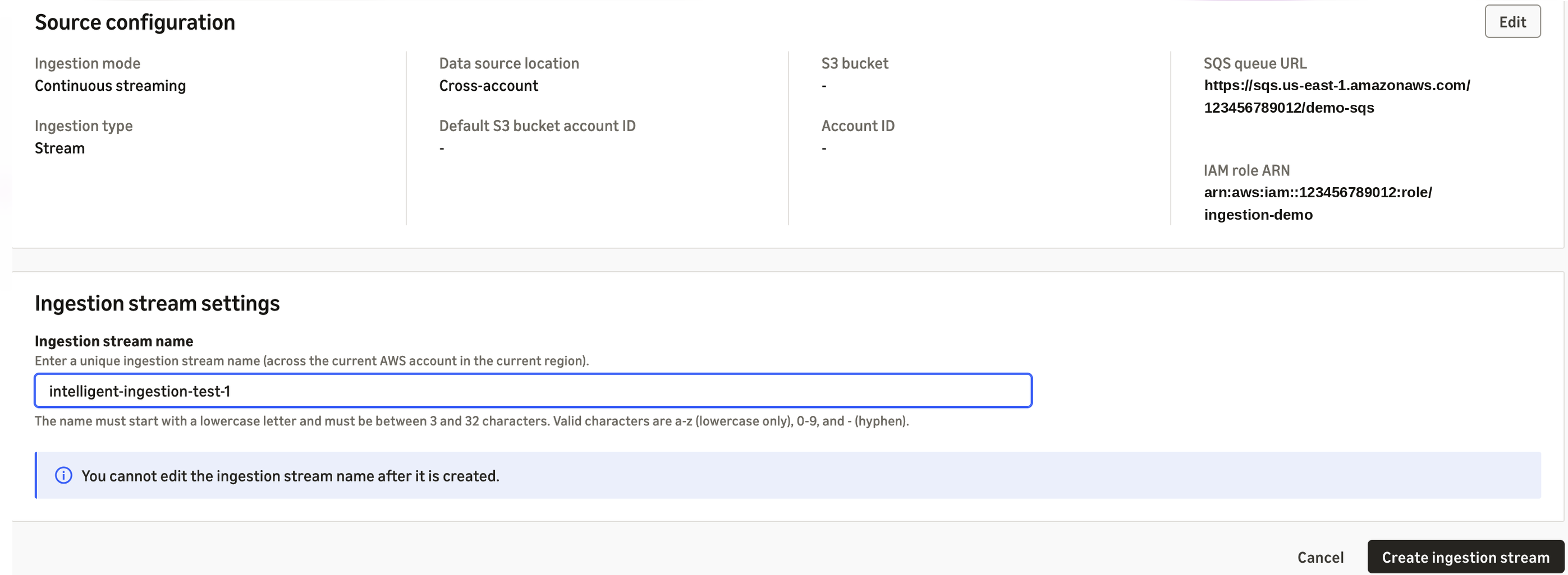
To get started, choose Create ingestion job and complete the configuration, and then choose Validate and continue. On this page, review the configuration, enter a name for the ingestion job or stream, and start the ingestion. The ingestion job or stream then appears on the Ingestion tab of the Amazon OpenSearch Serverless (NextGen) collection for a managerial view.
Figure 5: Reviewing and naming the ingestion job before starting
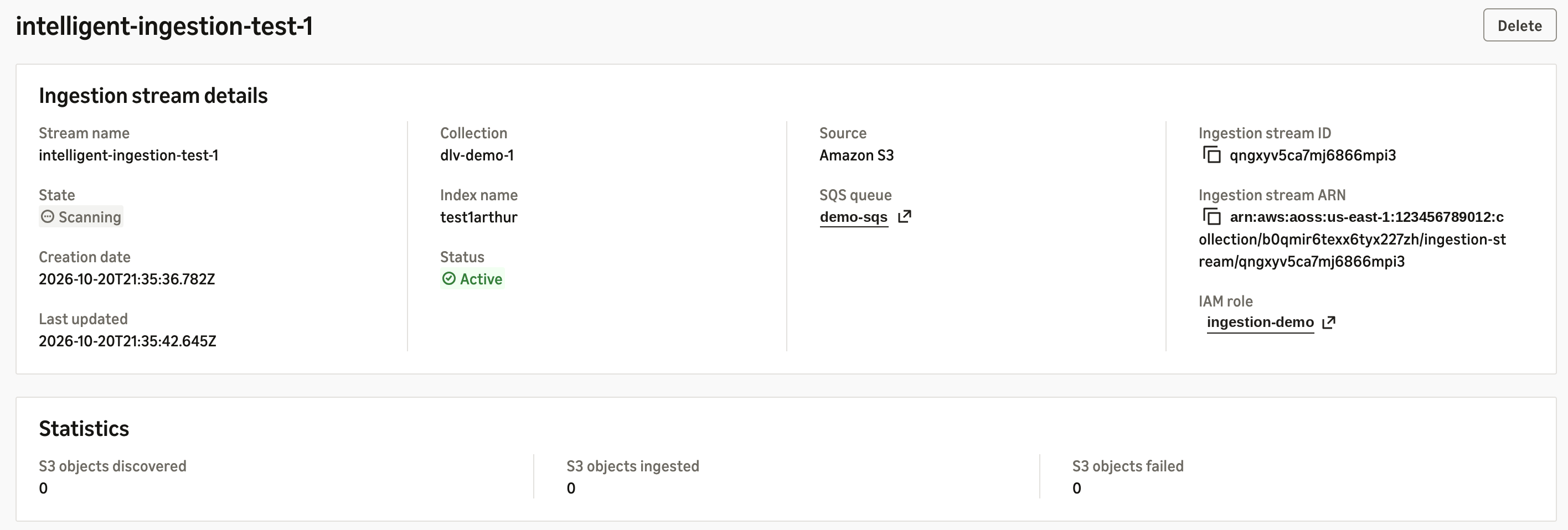
After it’s started, intelligent ingestion first scans the S3 bucket for data types and determines the processing mechanism for the content (structured data, unstructured data, or data with images). Intelligent ingestion automatically handles the tasks for the ingestion. You can monitor the number of documents it has scanned and indexed on the same page. Your data is now searchable in Amazon OpenSearch Serverless.
Figure 6: Monitoring documents scanned and indexed
Cost
Intelligent ingestion charges only for what you actually use.
Structured data such as JSON can be processed and ingested directly to OpenSearch Serverless for indexing. You pay for the standard OCU for each data ingestion worker while it is actively running. After the ingestion job completes, it automatically terminates and stops the billing.
Unstructured data such as PDF and Word documents requires additional parsing, chunking, and in some cases image understanding. Intelligent ingestion can automatically use the serverless indexing OCU (within your predefined limits) to extract text and chunk the pages into structured data. It charges the standard OCU rate, for example $0.24 per hour in US East (N. Virginia). This incurs an additional charge on top of structured data ingestion. Based on our internal testing, the one additional OCU can process 600 PDF pages per hour, which is $0.40 per 1,000 PDF pages processed and ready for ingestion. Intelligent ingestion uses Amazon Nova 2 Lite to translate the images within the PDF and Word files into semantic meanings. The Amazon Bedrock model inference cost is exactly the same as the public rates on Amazon Bedrock for Nova 2 Lite: $0.30 per 1M input tokens and $2.50 per 1M output tokens. Based on our internal testing, every 1,000 images consumes 0.5M input tokens on average, and 0.5M output tokens on average. You pay around $1.40 to process 1,000 images.
Clean up
To avoid future charges, delete the resources you created for this walkthrough. Delete any Ingestion Streams you created, then delete the OpenSearch collection and the sample documents in your S3 bucket if you no longer need them. Ingestion Jobs stop consuming capacity after they complete.
Conclusion
In this post, we showed how Amazon OpenSearch intelligent ingestion turns enterprise documents in Amazon S3 into RAG-ready intelligence without an ingestion pipeline to manage. You choose a source, a processing behavior, and a destination. Intelligent ingestion then parses your documents, describes their images, chunks the content, generates vector embeddings, and indexes the results. It scales with your workload and charges only for active processing. What once took weeks of pipeline engineering now takes only a few clicks or one API call, so your team can focus on the search and generative AI experiences your users need. Intelligent ingestion is available today for Amazon OpenSearch Serverless (NextGen) collections, with Amazon S3 as the data source, in six supported AWS Regions.
В неделя избираме седмия президент на България, което звучи почти митологично. Седмият син на седмия син се ражда с особени способности – лекува, вижда невидимото, предсказва бъдещето, в някои фолклорни традиции прави чудеса.
За седмия ни президент изискванията са по-скромни. Трябва просто да бъде избран. Но понеже сме в България и всичките до един сме синове на юнашко племе, успяваме и простото да направим сложно.
На 25 октомври гласуването е задължително (както впрочем и на всички избори от 26 май 2016 г. насам, нищо че не сте разбрали, понеже никой не ви е санкционирал, когато не сте гласували). За победа още на първия тур обаче не стига просто някоя от кандидатпрезидентските двойки да получи повече гласове от другите. Не. Трябва да е получила повече от половината действителни гласове и освен това в изборите да са участвали повече от половината избиратели (ама нали са задължителни изборите, не трябва ли да участват всички избиратели, питат неразбралите от задния ред). Ако това не стане, седмица по-късно двойките с най-много гласове отиват на балотаж.
Тоест в неделя избираме президент. Но по всяка вероятност всъщност ще избираме между кого ще избираме другата неделя.
Така или иначе избираме.
И понеже изборите са утре, вижте пък ние какво сме ви избрали за четене в „Тоест“ тази седмица.
Александър Драганов в „Кафе, боб и предизборни прогнози“ се захваща с любимото упражнение на политолози и социолози преди всеки вот – прогнозиране. Прави го, разбира се, с необходимата доза самоирония и с ясното съзнание, че между социологическо проучване, политически анализ, гледане на кафе и хвърляне на боб понякога разликата се установява чак след изборите.
Емилия Милчева пък гледа една стъпка по-нататък – към вероятния балотаж, защото игрите около него надхвърлят самия избор за президент. Кой срещу кого, кой зад кого, кой за кого и най-вече кой какво печели от подреждането. Самият факт, че ГЕРБ и ДПС нямат кандидати, но се говори, че за балотажа стягат редиците по тъчлинията с подкрепа за една конкретна кандидатка, която не е Ваня Великова, говори достатъчно.
А докато всички гледаме кой зад кого ще застане след изборите, тази седмица видяхме и кой застава между журналист и политик. В четвъртък вечер служител на НСО повали на земята Соня Колтуклиева, след като тя отвори вратата на автомобила на председателката на Народното събрание Михаела Доцова, за да ѝ зададе въпрос. Каквото и да мислим за журналистическите методи на ПИК и конкретно на Колтуклиева, физическата сила срещу журналист не става по-приемлива според това дали харесваме журналиста. Чак не ми се вярва, че доживях целият ми либерално-жълтопаветен балон да е Je suis Соня Колтуклиева, но такива са обратите на демокрацията.
А понеже обратите напоследък не са само вътрешнополитически, Искрен Иванов гледа към Черно море. В анализа си „България между член 4 и страха от Русия“ той поставя въпроса докъде може да стигне войната, без формално да е стигнала до нас. Русия няма непременно нужда от пряк сблъсък с НАТО. Достатъчна е някаква провокация, виждали сме го и друг път. Важно е обаче ние как ще реагираме и дали изобщо имаме готовност за реакция.
От геополитическия страх преминаваме ведро към телевизионния ужас „Ергенът“, който изгрява по екраните ни всяка пролет и есен. В текста си „Любов в ада“ Вера Краузе пита какво става, когато насилието, мизогинията и ксенофобията се превърнат в телевизионен формат, а прекрачването на граници – в зрителско очакване. Къде свършва забавлението, чия е отговорността и колко пъти трябва да видим нещо, за да спрем да го гледаме.
За щастие, има и други екрани. В рубриката „Игромислие“ Миглена Николчина този път събира поезията и видеоигрите. На пръв поглед странна двойка. На втори – не чак толкова. Оказва се, че стихотворението може да бъде ключ към играта, книгата – магически предмет, а поезията – съвсем буквално част от света, който трябва да разчетем, за да продължим напред.
Още една редовна рубрика имаме тези седмица – „Тези хора“, в която Ина Иванова разговаря с Мирослава Кацарова за музиката, стила, вкуса, Пловдив, приятелството, ските и свободата. „В музиката се откриваш като свободен човек“, казва Мирослава. Не е лошо да започнем да се търсим малко повече, че да вземем да се намерим най-накрая и да се даврандисаме.
От търсене какво да прави по време на пандемията, Стефан Иванов попада в съда като съдебен заседател. От известно време ни обещава, че ще ни разкаже за този период, и ето, дойде моментът. В няколко текста ще прочетем за професията съдебен заседател, която всъщност не е професия. Поредицата е личен разказ отвътре за институция, която познаваме отлично от американските филми и изумително слабо от нашата действителност. Българските съдебни заседатели всъщност имат права, равни на тези на съдиите. Решават за вината, за наказанието, а понякога даже могат да надделеят над съдията.
И на финала нещо важно: „Тоест“ съществува, защото го четете. Но съществува и защото част от вас го подкрепят финансово. За да можем да продължим да правим медия, в която никой не казва „айде, пускай да върви“, имаме нужда от вас. За всекидневната ни журналистическа работа няма проектно финансиране, няма голям собственик, няма спасител. И уви, няма седми син на седми син. Имаме си вас, нашите читатели.
Ако четете „Тоест“ редовно и можете да си го позволите, подкрепете ни с малко месечно дарение.
И в неделя гласувайте, а също така, като излезете от секцията, призовете своя вътрешен Доналд Тръмп, помахайте ведро и козирувайте тържествено на въображаеми хора някъде наоколо в живота.
Organizations that store analytics data on AWS often need two things at once. The first is fine-grained access control that limits each person to only the data they are authorized to see. The second is auditability down to the individual user level so that every query is traceable to the person who ran it rather than to a shared AWS Identity and Access Management (IAM) role.
AWS IAM Identity Center Trusted Identity Propagation (TIP) meets both requirements. A user signs in once, and that identity propagates from the client application through the query engine to Lake Formation and the storage layer, so that every request is authorized as the actual user and every query is logged in AWS CloudTrail.
AWS now extends TIP across Regions: IAM Identity Center replicates its identity objects such as users, groups, and session information to every AWS Region that you choose, so services across the stack can recognize the same user identity even when they span different Regions.
In this post, the producer shares data from the Asia Pacific (Sydney) Region (ap-southeast-2) and the consumer queries it from the South America (São Paulo) Region (sa-east-1) as themselves. We cover two cases that follow the same pattern. In Case 1, you share Amazon Simple Storage Service (Amazon S3) data governed by Lake Formation, queried from Amazon SageMaker Unified Studio (Athena). In Case 2, you share Amazon Redshift data through a datashare registered to the AWS Glue Data Catalog, queried from Amazon Redshift Serverless.
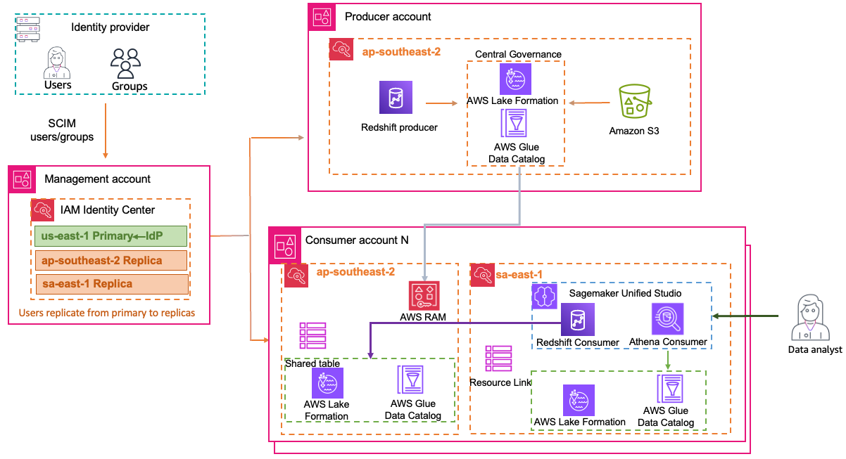
Figure 1: Cross-Region and cross-account architecture
Starting on the left of the diagram, your identity provider syncs users and groups into AWS IAM Identity Center through the System for Cross-domain Identity Management (SCIM) protocol. Running as an organization instance in the management account, IAM Identity Center replicates those identities to every Region in use. In the center, the producer account in Sydney uses AWS Lake Formation to centrally govern both Amazon S3 and Amazon Redshift data. When the producer shares a table or database, that share flows to the consumer account in São Paulo, shown on the right, where a resource link makes the shared data queryable as if it were local. On the right, the data analyst signs in to Amazon SageMaker Unified Studio with corporate credentials. With Trusted Identity Propagation enabled, the analyst’s identity travels with every request to Lake Formation. Lake Formation authorizes each query based on who the user is rather than which IAM role they assumed.
The example uses three accounts across three Regions. The producer account runs Amazon S3, AWS Glue Data Catalog, Lake Formation, and Amazon Redshift Serverless in ap-southeast-2 (Sydney). The consumer account queries from sa-east-1 (São Paulo) using SageMaker Unified Studio or Amazon Redshift. IAM Identity Center runs in us-east-1 (Virginia) in the management account.
Cross-account sharing through Lake Formation can span AWS Organizations, but the TIP integration adds a tighter requirement. For the user’s identity to propagate, the producer and consumer accounts must be in the same organization and share the same organization instance of IAM Identity Center. You can repeat the consumer steps to add more accounts or Regions. With this launch, you can query that shared data from a different Region while Lake Formation authorizes every request as the actual user.
How the pieces fit together
Four capabilities underpin this architecture. IAM Identity Center provides a single identity plane across Regions, so the same users and groups are available in every account. Each service in the stack supports Trusted Identity Propagation, so the user’s identity flows from the client application to Lake Formation without falling back to IAM roles. Corporate sign-in through IAM Identity Center makes that identity available across Regions and accounts within the organization. Finally, AWS Resource Access Manager (AWS RAM) shares and resource links bridge the Region gap so the consumer can query data cataloged in the producer’s Region.
Prerequisites
Before you begin, make sure that you have the following in place:
The producer account and consumer account are in the same organization.
An organization instance of IAM Identity Center, with users and groups provisioned.
You have permissions to administer AWS Lake Formation, AWS Glue, AWS RAM, Amazon Simple Storage Service (Amazon S3), Amazon SageMaker Unified Studio, and Amazon Redshift in the relevant accounts.
In the producer Lake Formation Data catalog settings, the Use only IAM access control options should be cleared.
The AWS services used in this post are integrated with AWS IAM Identity Center in both the producer and consumer accounts, across the Regions used in this walkthrough. See Trusted identity propagation use cases for more information.
Case 1: Share S3 data (Lake Formation)
In this case, the S3 data and its catalog stay in the producer’s account and Region the whole time, with Lake Formation governing them in Sydney (ap-southeast-2). What crosses Regions is the query itself. The consumer, in a different account, connects from São Paulo (sa-east-1) and queries that same data through Amazon Athena (through SageMaker Unified Studio). This is a federated query pattern: the data stays in place, and only the query crosses Regions. That split (catalog and data in one Region, client and query in another) is what makes this genuinely cross-Region, not just cross-account.
Part 1: Producer account (Sydney, ap-southeast-2)
Region note: the walkthrough uses ap-southeast-2 (producer) and sa-east-1 (consumer and query). Substitute your own Regions and account IDs where you see placeholders. All cross-account Lake Formation grants must be made in the producer Region. The only exception is the resource link and its Describe grant, which are created in the consumer’s query Region.
Step 1.1: Create the sample data file
Create a file named customers.csv with the following content.
Open the Amazon S3 console in the producer account (ap-southeast-2).
Choose Create bucket, enter a unique name (for example, amzn-s3-demo-sydney-lakehouse-bucket), and choose Create bucket.
Open the bucket, create a folder named customers, and upload customers.csv into it.
Step 1.3: Create the Lake Formation registration role (with sts:SetContext)
Create an IAM role that Lake Formation assumes to read the S3 bucket. This role is used when registering the data lake location and for vending credentials, including for TIP. Don’t use the Lake Formation service-linked role. It doesn’t include sts:SetContext.
Open the IAM console, choose Roles, then Create role.
For Trusted entity type, choose Custom trust policy and paste the following trust policy.
Choose Next, skip attaching managed policies, and choose Next.
Name the role (for example, LakeFormation-DataLocation-role) and choose Create role.
Open the role, choose Add permissions, then Create inline policy, and paste the following permissions policy.
Name the inline policy (for example, LF-S3Access) and save it.
Note: The sts:SetContext action in the trust policy is required for TIP. The Lake Formation service-linked role doesn’t include it, which is why a custom role is required here.
Step 1.4: Register the S3 location in Lake Formation
Under Data Catalog, choose Tables, Add table, then Add table manually.
For Table name, enter customers.
For Database, choose sydney_lakehouse.
For the data store, choose Amazon S3 and set the location to s3://amzn-s3-demo-sydney-lakehouse-bucket/customers/.
For the data format, choose CSV with comma (,) as the delimiter.
Define the schema using the following columns.
Add the table property skip.header.line.count with value 1 to skip the CSV header row.
Review and choose Create.
Column name
Data type
customer_id
string
first_name
string
last_name
string
email
string
city
string
state
string
signup_date
string
When you create the table as CSV on the console, define all columns as string. The CSV serializer/deserializer used for this table doesn’t parse typed columns such as date or bigint reliably. Cast values in your queries as needed (for example, CAST(signup_date AS date)).
Step 1.7: Grant DATABASE permission to the external (consumer) account
Under Principals, choose External accounts and enter the consumer account ID (<CONSUMER_ACCOUNT_ID>).
Choose Named Data Catalog resources. For Databases, choose your database, in this post sydney_lakehouse.
For Database permissions, select Describe, and select Describe under Grantable permissions.
Choose Grant.
Step 1.8: Grant TABLE permission to the external (consumer) account
Choose Permissions, Data lake permissions, then Grant.
Under Principals, choose External accounts and enter <CONSUMER_ACCOUNT_ID>.
Choose Named Data Catalog resources. For Databases choose sydney_lakehouse. For Tables choose customers.
For Table permissions, select Select and Describe, and select the same under Grantable permissions.
Choose Grant.
Step 1.9: Grant DATABASE permission to the IAM Identity Center group/user
Choose Permissions, Data lake permissions, then Grant.
Under Principals, choose IAM Identity Center and select the group or user (for example, admin).
Choose Named Data Catalog resources. For Databases choose your database, in this post sydney_lakehouse.
For Database permissions, select Describe.
Choose Grant.
Step 1.10: Grant TABLE permission to the IAM Identity Center group/user
Choose Permissions, Data lake permissions, then Grant.
Under Principals, choose IAM Identity Center and select the group or user (for example, admin).
Choose Named Data Catalog resources. For Databases choose your database and table, in this post sydney_lakehouse and for Tables choose customers.
For Table permissions, select Select and Describe.
Choose Grant.
Note: Because the accounts share one organization instance of IAM Identity Center, the producer can grant the IAM Identity Center group directly on the underlying table. The consumer only grants Describe on the local resource link (Step 2.3).
At this point, the producer side is complete. You have the necessary Lake Formation permissions for both the consumer account and your users. To verify, open Data lake permissions in the Lake Formation console and confirm you see four grants covering the database and table.
Part 2: Consumer account
In this part, you switch to the consumer account to accept the AWS RAM share, create a resource link that points back to the shared database, and grant your users access to it. After these steps, the consumer account is ready to query the producer’s data from a different Region.
Step 2.1: Accept the AWS RAM share (Sydney Region)
Open the AWS RAM console and switch to ap-southeast-2 (Sydney).
Under Shared with me, choose Resource shares.
Select the resource share from the producer account and choose Accept resource share.
Step 2.2: Create the resource link (sa-east-1 Region)
Under Data catalog, choose Databases, then Create resource link.
For Resource link name, enter a name, for example rl_sydney_s3_datalake.
For Shared database’s Region, choose Asia Pacific (Sydney)ap-southeast-2.
For Shared database, choose your database. In this post the database is called sydney_lakehouse.
Shared database’s catalog ID populates automatically (the producer account).
Choose Create.
Step 2.3: Grant Describe on the resource link to the IAM Identity Center group/user
In the Lake Formation console (sa-east-1), choose Permissions, Data lake permissions, then Grant.
Under Principals, choose IAM Identity Center and select the group or user (for example, admin).
Choose Named Data Catalog resources. For Databases choose rl_sydney_s3_datalake.
For Resource link permissions, select Describe.
Choose Grant.
Part 3: SageMaker Unified Studio (sa-east-1)
With the producer and consumer accounts configured, you now set up SageMaker Unified Studio in the query Region and run the cross-Region query.
Step 3.1: Create the SageMaker Unified Studio domain
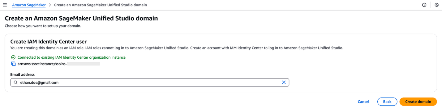
Open the Amazon SageMaker console in sa-east-1, choose Unified Studio, then Create domain. See the SageMaker Unified Studio administration guide for the quick setup. Because your IAM Identity Center integration is already complete, you can specify an IAM Identity Center user in the domain configuration settings.
Figure 2: Adding an SSO user in the Amazon SageMaker Unified Studio domain
To enable Trusted Identity Propagation (TIP) in SageMaker Unified Studio, refer to the following sections in this post:
Enable TIP in SageMaker Unified Studio.
Enable user access for SageMaker Unified Studio domain.
Add project members.
Create a SQL analytics project in Unified Studio. For this post, we use the project name my_project_idc.
Step 3.2: Enable TIP
Sign in to the SageMaker Unified Studio portal by choosing Sign in with SSO as an IAM Identity Center user.
Figure 3: Sign in with SSO in Amazon SageMaker Unified Studio
Open the project (my_project_idc) and go to the Query Editor.
Under Catalogs, choose AwsDataCatalog.
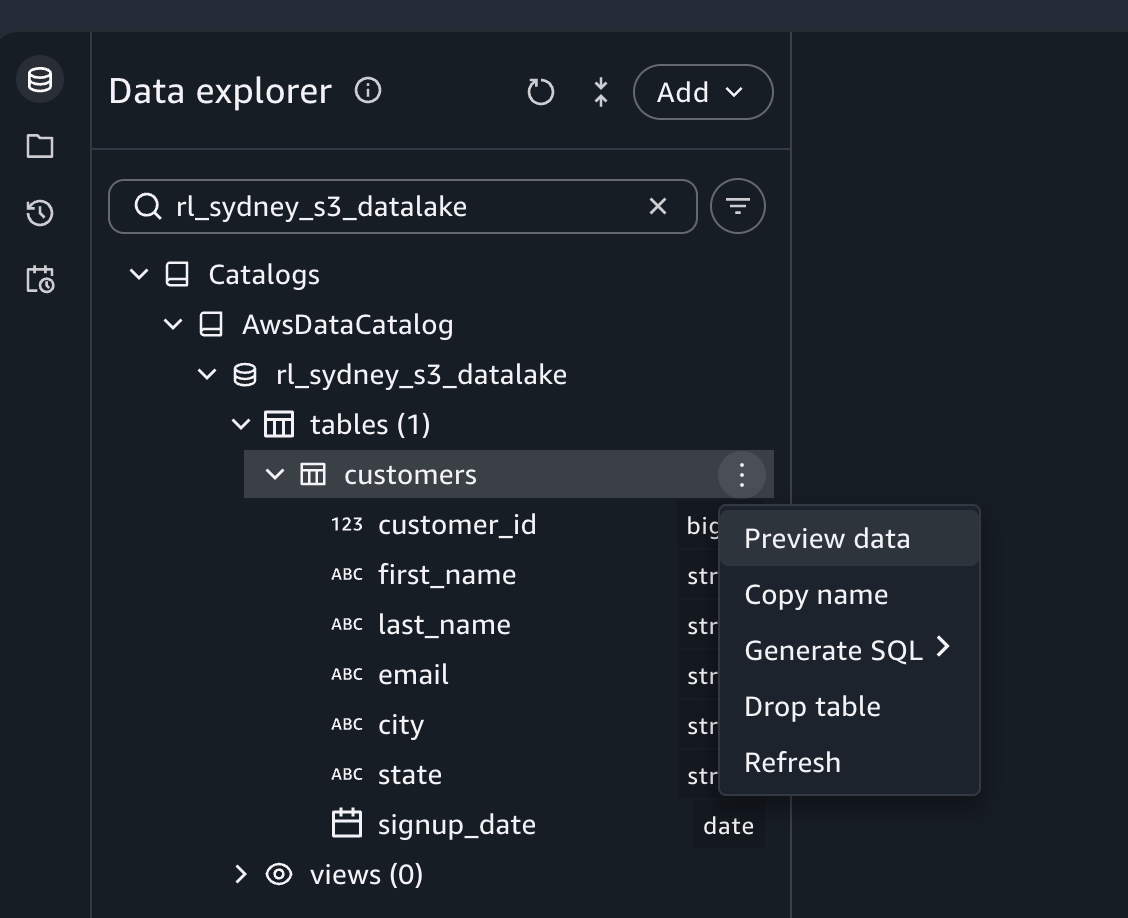
Choose rl_sydney_s3_datalake, then tables, and then select customers.
Choose the three dots next to the customers table and choose Preview data.
Figure 4: Access Amazon S3 data in Amazon SageMaker Unified Studio
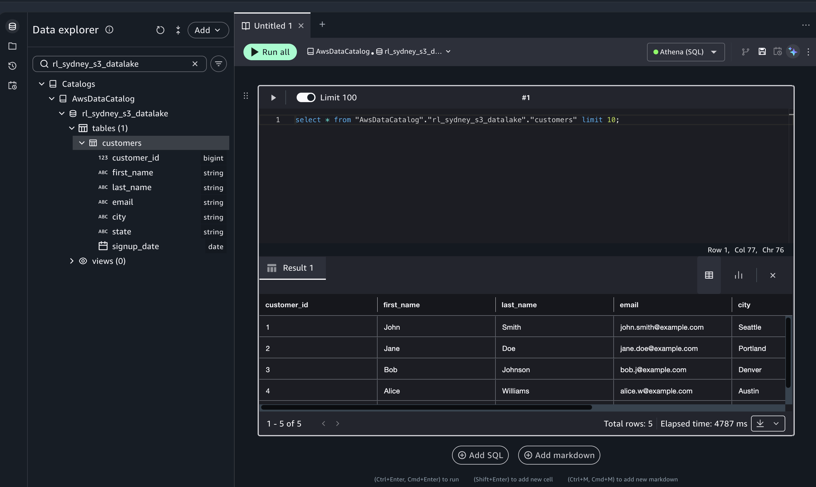
The query auto-runs using the Athena compute, as shown in the following screenshot:
SELECT * FROM "AwsDataCatalog"."rl_sydney_s3_datalake"."customers" LIMIT 10;
Figure 5: Preview Amazon S3 data in Amazon SageMaker Unified Studio
The customer data from the producer S3 bucket in Sydney is returned, governed by Lake Formation and accessed through the resource link in sa-east-1, with the user identity propagated through TIP.
Case 2: Share Amazon Redshift data using AWS Glue federated catalog
This case follows the same centralized-catalog pattern as Case 1, but the consumer queries the data with Amazon Redshift Serverless instead of Athena. The analyst runs these queries from SageMaker Unified Studio using its Amazon Redshift query experience.
Part 1: Producer account (Sydney, ap-southeast-2)
Make sure that your Amazon Redshift consumer cluster is configured with IAM Identity Center in both ap-southeast-2 and sa-east-1 Regions. If you need to review the procedure, see Integrate Identity Provider (IdP) with Amazon Redshift Query Editor V2 using AWS IAM Identity Center for seamless Single Sign-On.
Step 1.1: Register a serverless namespace to the AWS Glue Data Catalog
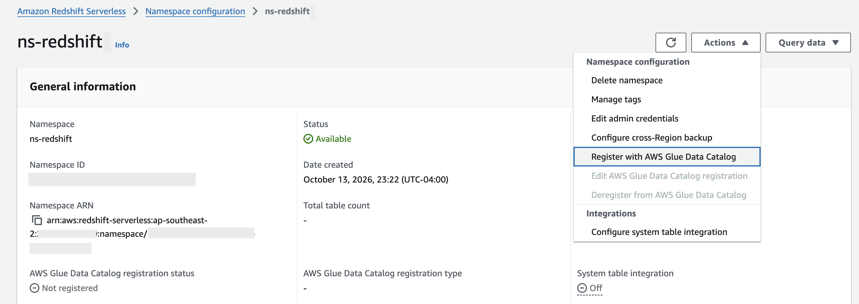
On the navigation menu, choose Redshift Serverless. The Namespaces / Workgroups section shows your namespaces and workgroups for the current Region.
Choose the name of the namespace you want to register.
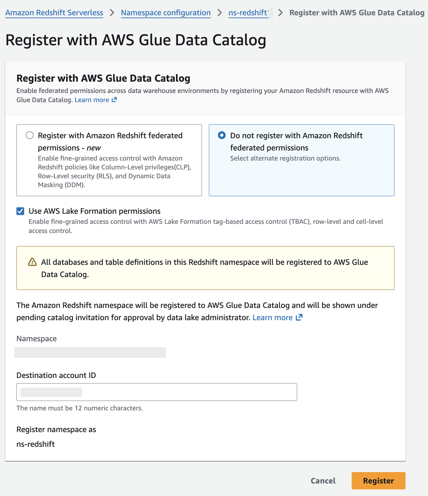
From Actions, choose Register to AWS Glue Data Catalog.
Figure 6: Amazon Redshift Serverless namespace to register with the AWS Glue Data Catalog
Choose Do not register with Amazon Redshift federated permissions.
Select Use AWS Lake Formation permissions.
For Destination account ID, enter the producer account ID (<PRODUCER_ACCOUNT_ID>), the account that will hold the catalog.
Choose Register. You are taken to the AWS Lake Formation console.
Figure 7: Register the Amazon Redshift Serverless namespace with the AWS Glue Data Catalog
Follow the catalog creation process in Lake Formation. See Creating Amazon Redshift federated catalogs and follow these steps:
Review a namespace invitation and accept it.
Create a federated catalog.
Step 1.2: Grant DATABASE permission to the external (consumer) account
In the Lake Formation console (ap-southeast-2), choose Permissions, Data lake permissions, then Grant.
Under Principals, choose External accounts and enter <CONSUMER_ACCOUNT_ID>.
Choose Named Data Catalog resources. For Catalogs/Databases, choose the federated database (for example, ns-redshift/dev, schema sales_schema).
For Database permissions, select Describe (and Describe under Grantable permissions).
Choose Grant.
Step 1.3: Grant TABLE permission to the external (consumer) account
Choose Permissions, Data lake permissions, then Grant.
Under Principals, choose External accounts and enter <CONSUMER_ACCOUNT_ID>.
Choose Named Data Catalog resources and select the shared table (for example, store_sales).
For Table permissions, select Select and Describe (and the same under Grantable permissions).
Choose Grant.
Step 1.4: Grant DATABASE permission to the IAM Identity Center group/user
Choose Permissions, Data lake permissions, then Grant.
Under Principals, choose IAM Identity Center and select the group or user.
Choose Named Data Catalog resources and select the federated database (schema).
For Database permissions, select Describe.
Choose Grant.
Step 1.5: Grant TABLE permission to the IAM Identity Center group/user
Choose Permissions, Data lake permissions, then Grant.
Under Principals, choose IAM Identity Center and select the group or user.
Choose Named Data Catalog resources and select the shared table (for example, store_sales).
For Table permissions, select Select and Describe.
Choose Grant.
Part 2: Consumer account
At this point, the producer side for Case 2 is complete. To verify, open Data lake permissions in the Lake Formation console and confirm you see four grants covering the federated database and shared table.
In this part, you switch to the consumer account to accept the AWS RAM share, configure the IAM role for cross-Region Amazon Redshift access, and set up TIP so that users can query the producer’s Amazon Redshift data from a different Region.
Step 2.1: Accept the AWS RAM share (Sydney Region)
Select the resource share from the producer account and choose Accept resource share.
Step 2.2: Update the trust relationship for the IAM role
Navigate to the IAM role (IAMIDCRedshiftRole) created in this post.
Make sure the trust policy includes Amazon Redshift and Amazon Redshift Serverless for sts:AssumeRole and sts:SetContext, as shown in the following policy:
Note: These actions require "Resource": "*" because they are used for catalog-level discovery, which does not support resource-scoped permissions. Lake Formation column-level and row-level grants still enforce least-privilege access to the underlying data.
Step 2.4: Set up cross-Region Trusted Identity Propagation (TIP) access in Amazon Redshift
Sign in to the Amazon Redshift console using the admin role.
Navigate to Query Editor V2.
Choose the options menu (three dots) next to the cluster and choose Create connection.
Connect as the admin user and run the following command to create an external schema that points to your cross-Region AWS Glue Data Catalog:
Syntax:
CREATE EXTERNAL SCHEMA <schema_name>
FROM DATA CATALOG
DATABASE '<glue_db_name>'
REGION '<producer region where glue Data Catalog lives>'
CATALOG_ID '<catalog_name>';
Example:
CREATE EXTERNAL SCHEMA redshift_cross_region_tip
FROM DATA CATALOG
DATABASE 'sales_schema'
REGION 'ap-southeast-2'
CATALOG_ID '123456789012:ns-producer-redshift-syd/dev';
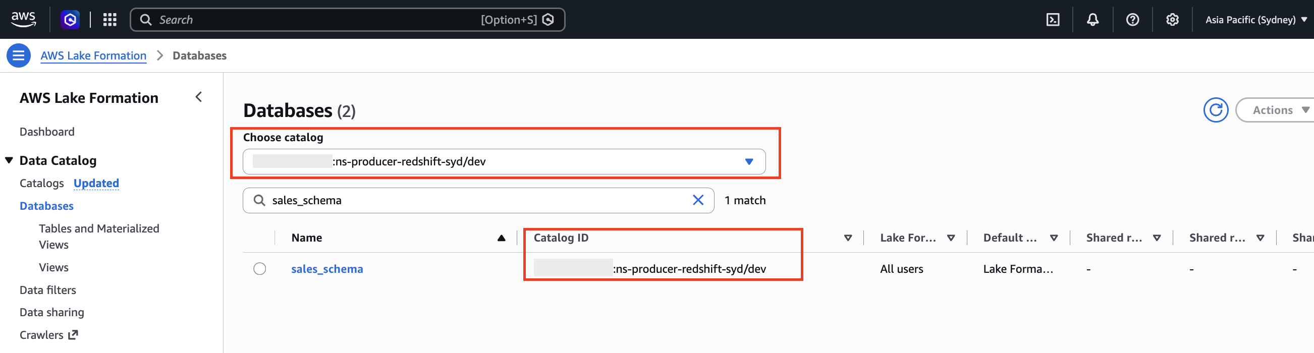
You can get this catalog_name information from the producer account Lake Formation in the Sydney Region. Navigate to Databases on the left and choose the respective Amazon Redshift catalog ID from the drop-down.
Figure 8: AWS Lake Formation showing the catalog ID of the Amazon Redshift namespace registered with the AWS Glue Data Catalog
Grant the IAM Identity Center group access to the external schema.
GRANT USAGE ON schema redshift_cross_region_tip TO ROLE "AWSIDC:admin";
Step 2.5: Query the data from Amazon Redshift Query Editor V2
In Query Editor V2, choose the options menu (three dots) next to the cluster and choose Edit connection, and for authentication, select IAM Identity Center.
A pop-up redirects you to your IdP login page. Enter your IdP credentials.
After successful authentication, you are redirected to Query Editor V2 as an IAM Identity Center user.
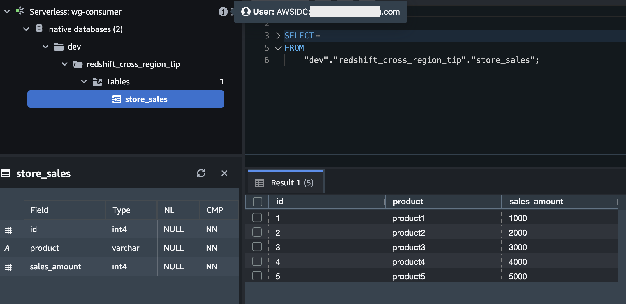
Run the following query.
SELECT * FROM "dev"."redshift_cross_region_tip"."store_sales";
Figure 9: Query cross-Region, cross-account data using Amazon Redshift Query Editor V2
Step 2.6: Query the data from SageMaker Unified Studio
For a consumer cluster to use in SageMaker Unified Studio, you need to tag the Amazon Redshift cluster or workgroup with one of the following options. Choose one before proceeding.
Option 1 – Add a tag to allow only a specific SageMaker Unified Studio project to access it: AmazonDataZoneProject=<projectID>
Option 2 – Add a tag to allow all SageMaker Unified Studio projects in this account to access it: for-use-with-all-datazone-projects=true
After the Amazon Redshift cluster or workgroup has a tag, continue with the following steps.
Sign in to the SageMaker Unified Studio portal by choosing Sign in with SSO as an IAM Identity Center user.
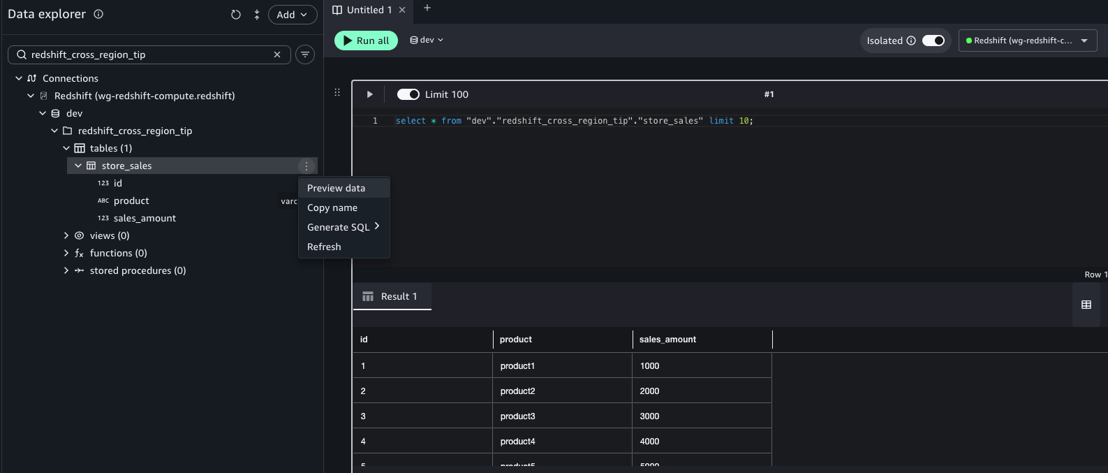
In SageMaker Unified Studio, navigate to Query Editor and expand Connections.
Choose redshift_cross_region_tip, then tables, and then select store_sales.
Choose the three dots next to the store_sales table and choose Preview data. The query auto-runs using the Amazon Redshift compute, as shown in the following screenshot:
Figure 10: Query data using Amazon Redshift compute in Amazon SageMaker Unified Studio
The Amazon Redshift data shared from the producer in Sydney is returned. It is governed and centralized in one account and Region (ap-southeast-2) using Lake Formation and accessed from the consumer account in a second Region (sa-east-1), with the user identity propagated through TIP.
Both cases use the same Region split. The catalog and the data stay in the producer Region (Sydney), and only the client and the query run from the consumer Region (São Paulo). They differ only in the query engine. Case 1 uses Amazon Athena, and Case 2 uses Amazon Redshift Serverless. That difference in engine is also what changes their cross-Region behavior. With Athena (Case 1), queries work cross-Region without additional constraints. However, if you use an Amazon Redshift datashare, the Amazon Redshift query engine must be in the same Region as the Amazon Redshift namespace.
Clean up
To avoid ongoing charges, remove the resources that you created.
Consumer account:
Delete the SageMaker Unified Studio project and domain (Case 1).
Delete the Amazon Redshift Serverless workgroup and namespace (Case 2).
In Lake Formation (sa-east-1), delete the resource links (rl_sydney_s3_datalake, rl_redshift_cross_db_tip).
Revoke any Lake Formation grants you created and, if applicable, leave/deny the AWS RAM share.
Producer account:
Revoke the Lake Formation grants to the consumer account and to the IAM Identity Center group.
Revoke the AWS RAM share.
Deregister the S3 data lake location, and delete the customers table and the sydney_lakehouse database.
Empty and delete the S3 bucket.
Deregister the Amazon Redshift namespace from the AWS Glue Data Catalog and delete the federated catalog (Case 2).
Delete the IAM roles you created (LakeFormation-DataLocation-role, IAMIDCRedshiftRole).
Conclusion
In this post, you configured AWS Lake Formation Trusted Identity Propagation so that data governed and shared in one Region (Sydney) can be queried from another Region (São Paulo). Lake Formation cross-account grants are made in the producer Region, and the consumer reaches the shared data from the query Region in the way that fits each engine. For Amazon S3 data queried through Amazon Athena (Case 1), the consumer creates a resource link in the query Region that points back to the shared database. For Amazon Redshift data shared through a datashare and AWS Glue federated catalog (Case 2), the consumer instead creates an external schema in Amazon Redshift that references the producer’s Glue Data Catalog directly in the producer Region. No resource link is required. In both cases, because access is authorized against the user’s IAM Identity Center identity rather than a shared role, you get least-privilege access, per-user auditability in AWS CloudTrail, and a single place to manage permissions.
To add more consumer accounts or query Regions, repeat the consumer-side steps for the relevant case: accept the AWS RAM share in the producer Region, then either create a resource link in the query Region and grant Describe on it to your IAM Identity Center principals (Amazon S3 and Athena), or create an external schema that references the producer’s Glue catalog and grant usage to your IAM Identity Center principals for Amazon Redshift.
As a next step, review the Trusted Identity Propagation supported applications and services to plan which services in your stack to enable with TIP, using the Lake Formation cross-account sharing documentation as a reference.
Quasar connects a proposed API change with observed references in consumer repositories, giving the producer evidence for a release decision
At Netflix, shared Java libraries support applications developed across a large, independently evolving repository ecosystem. A library change begins in one repository, but its impact can reach many others. Producers can see the API diff in front of them. What they often cannot see is who still depends on the symbols that changed.
The need for that visibility grows as coding agents take on more of the software development lifecycle. An agent can accelerate a local edit, but without cross-repository context it cannot judge downstream risk or help plan consumer migrations. The evidence a producer uses to assess a change can also guide the agent working on it.
Consider a common case: removing a deprecated API. Deprecated entry points expand the surface producers must test, document, and support, and they can constrain how a library evolves.
Suppose a replacement has been available for several releases and the old method cannot express options required by new behavior. The library’s tests pass, and a compatibility checker flags the removal. The producer still cannot answer the questions that determine what to do next:
Does any consumer still call this method?
Are consumers concentrated on one version or spread across several generations?
Does another library implement or wrap the API, multiplying its impact?
Is direct coordination sufficient, or does this require a deprecation and migration campaign?
At small scale, producers can ask nearby teams or search a handful of repositories. Across many repositories, it is harder to find every caller of a method and the library version each one uses. Those answers are scattered across consumer codebases and builds.
Without that evidence, a producer may release a breaking change and discover the impact through consumer failures, or preserve an old API indefinitely because the risk is unknown. Libraries need to evolve, and their producers need evidence that helps them do so intentionally.
We built Quasar to index symbol definitions and references across Netflix repositories. For library producers, that shared index helps answer two questions:
What changed in the library’s public API?
Which repositories use the exact symbols that changed?
The first identifies a potentially incompatible change. The second estimates its observed blast radius. Together, they turn a generic compatibility warning into evidence a producer can act on before merging or releasing.
From API Changes to Consumer Impact
Existing techniques each see a different part of the problem. Binary and source compatibility tools identify contract changes, but cannot tell who uses the changed API. Dependency graphs show declared reach, but cannot prove that code calls a particular method. Text search may miss overloads, inheritance, or the artifact version behind a call. Consumer builds provide strong validation, but running them across the fleet is expensive.
Quasar builds on SCIP, an open interchange format for semantic code intelligence. Language-specific indexers encode definitions, references, and relationships using stable symbol identifiers. Quasar retains API definitions for library versions and commits alongside references from consumer repositories. That shared identity lets it connect an API change in one repository to exact usages elsewhere, even when those repositories were indexed independently.
On each enrolled CI build, language-specific indexers submit SCIP indexes to Quasar’s ingestion service. It writes API definitions and consumer references as Parquet in Amazon S3, retaining the symbol identity, dependency version, and source location needed to investigate a change.
During pull-request review, Quasar compares indexed base and head definitions and counts direct consumer references with Amazon Athena. Quasar exposes those findings through its REST and GraphQL APIs and MCP server; follow-up usage queries provide dependency-version breakdowns and source locations. A separate compatibility-impact assessment can also follow implementations and their callers when a producer supplies a changed JVM symbol.
Consider this simplified API change:
public interface Client {
- Result getLegacyValue(Request request);
+ Result getValue(Request request, Options options);
}
For a detailed compatibility-impact assessment of this removal, a producer-side tool supplies the old method descriptor. Quasar constructs its canonical symbol identity. This abridged excerpt from the direct-reference portion of Quasar’s Amazon Athena query shows the essential match:
SELECT c.change_id, 'DIRECT_REFERENCE' AS evidence_kind,
       r.scm_type, r.org, r.repo, r.dep_version, r.file_path
FROM requested_changes c
JOIN quasar.symbol_refs r
  ON r.symbol_canonical = c.target_canonical
requested_changes contains the API changes submitted by the producer. The SQL excerpt finds repositories that call the removed method. Quasar also checks implementations and calls through them, so it can count each affected repository once. It returns sample dependency versions and file locations to help investigate the result.
For the Client change, this tells the producer which repositories still use getLegacyValue, which versions they use, and where some of those calls occur. That helps the producer decide whether to coordinate a migration before removing the method.
Bringing the Analysis Before Release
Version-to-version comparison is valuable when planning an upgrade or writing a migration guide. Producers benefit even more when feedback arrives during code review.
For pull-request analysis, Quasar stores API definition snapshots keyed by commit. Given a base and head commit, it classifies symbols as added, removed, or signature-modified. Removals and modifications then become candidates for consumer-impact analysis.
An incompatible change is not automatically a high-risk change. Quasar reports the observed impact so the producer can decide what to do; it does not enforce a release policy. “No references observed” means only that Quasar found none in the indexed population. Reflection, configuration, dynamic loading, stale branches, or incomplete indexing can hide consumers. The result needs to show whether the requested commits were indexed, how fresh the consumer indexes are, and whether evidence was truncated.
Pull-request review requires indexed snapshots for the exact base and head commits. If either is unavailable, Quasar reports that it cannot compare them; it does not substitute a default-branch snapshot. This keeps a missing comparison from looking like a clean API diff.
Return to our Client change. This illustrative report brings together signals available through Quasar's API comparison, consumer-usage queries, and library-level criticality. It is not a literal response from one API:
An impact report shows 137 affected repositories distributed across library versions 4.2.1, 4.1.7, and 3.9.4.
The repository count is symbol-specific: in this example, 137 indexed repositories refer to the removed method. The version distribution reveals a dominant cohort on 4.2.1 and a smaller long tail still on 3.9.4. A producer can inspect affected repositories and retrieve indexed file paths, with line numbers where the index provides them. The JSON shows only two sample locations to keep the example readable. The filePath and lines shape mirrors Quasar's query contract. The tier is broader context about the library, inherited from its highest-criticality downstream application; it does not imply that all 137 callers are Tier 1.
Together, those signals change the producer’s plan. Instead of merging the removal and waiting for failures, the producer can retain and deprecate the old method, publish a migration path, coordinate a broader migration, and track the long-tail versions before removal. File paths and available line numbers turn that scope into a concrete work list for engineers or coding agents. The same API diff paired with weak or stale evidence would lead to a different action: refresh the indexes before deciding. The value is not merely detecting the removal; it is choosing a proportionate next step.
A pre-release workflow enriches API changes with consumer impact and evidence quality before the producer decides how to proceed
A Polyglot Foundation with SCIP
The shared SCIP format also lets Quasar index several language ecosystems. Each language indexer resolves its own code, while Quasar can use the resulting symbol identities to find references across repositories.
Conceptually, client-lib indexes Client#getLegacyValue(Request) as a definition, while checkout-service indexes a reference to the same symbol. Quasar can then connect the library API to its consumer across repositories.
Language-specific indexers emit SCIP definitions, references, and relationships into Quasar’s shared semantic graph.
Relationships are especially useful when generated code separates the API a producer owns from the symbols consumers invoke. For example, Quasar can trace a Protobuf definition through its generated Java members to the repositories that use them, even when consumer code never names the .proto element.
SCIP records symbols and their references; it does not determine whether an API change violates an ecosystem’s compatibility rules. Today, Quasar compares indexed JVM and Protobuf API definitions and traces Protobuf changes through generated Java to find affected repositories. A separate JVM compatibility-impact path uses breaks identified by a producer-side tool to query affected repositories. Go, Python, JavaScript/TypeScript, and Rust support usage queries, but Quasar does not yet assess their breaking API changes.
Moving Risk Assessment Earlier
Today, Quasar surfaces API-change findings on pull requests, including observed consumer counts and confidence. Producers can use its other queries to inspect dependency versions and source locations, with library criticality as broader context. Together, those signals support a decision before merge.
We want to move that context earlier. An agent writing library code should recognize when it is changing a public symbol and consult Quasar before the change becomes a pull request. Quasar’s APIs and Model Context Protocol (MCP) integration provide an access path, but access alone does not create awareness. The coding workflow must also recognize public API edits so the agent knows when to query impact and when to involve the producer.
Today Quasar assesses risk on a pull request. The future workflow gives agents consumer-impact context while they write code, before the pull request is opened.
Earlier guidance will not replace pull-request analysis. The PR assessment will still verify the concrete diff and catch changes that were not recognized during coding. Coverage, freshness, ambiguity, unsupported platforms, and truncation must travel through both checks in machine-readable form. An agent should not turn “no observed usages in the available index” into “safe to remove.”
Today, agents can query Quasar through MCP when prompted. We are working toward making that context part of the coding workflow, then using identified call sites to prepare migration changes. Quasar supplies semantic evidence, an agent reduces migration toil, and the library producer remains responsible for API and release decisions.
What We Learned
Building this workflow led us to four practical lessons.
Separate compatibility from reach. A removed method can break the API contract even when Quasar finds no callers. A list of affected repositories and their library versions shows the migration work ahead. Producers need both signals to choose a release path.
Make the evidence inspectable. A repository count is more useful with sample call sites and a version breakdown. The result also needs to show which commits were indexed, how fresh the consumer indexes are, and whether evidence was truncated. Otherwise, “no usage found” can be mistaken for proof that nobody is affected.
Keep usage and compatibility separate across languages. SCIP lets Quasar find symbol references in several ecosystems. Deciding whether an API change is breaking requires compatibility rules or a trusted producer-side signal for that ecosystem.
Bring evidence to the producer while choices are open. Pull-request findings can prompt a producer to retain an API, publish a migration path, or coordinate consumers before merge. Moving the same evidence into the coding workflow could shape the edit earlier. After release, it still helps locate consumers that need to migrate.
Today, Quasar indexes JVM, Go, Python, JavaScript/TypeScript, and Rust code for cross-repository usage analysis. It compares JVM APIs and traces Protobuf changes through generated Java. Producers can review change findings through Quasar’s REST and GraphQL APIs or its MCP server, then investigate affected repositories and call sites. We are extending this foundation toward more ecosystem-specific compatibility checks, deeper code-review integration, and agent-assisted consumer migrations that keep release approval with the producer.
Quasar is internal to Netflix, but the pattern is portable: index code semantically, retain API definitions, compare them at the point of change, query affected consumers, and report the quality of the evidence. Library producers need more than a compatibility verdict. They need to know who may be affected and have enough time to act before release.
A huge thank you to the Java Platform team at Netflix. Their expertise, collaboration, and support made this work possible
A video player seeking to the middle of a movie asks for a few megabytes. Under our old range caching, that one request could make Cloudflare pull 128 MiB from the origin and move it between data centers, sometimes after the viewer had already left. Range requests are how large files get delivered, and caching them naively easily leads to wasted network bandwidth and wasted disk operations when running a CDN at scale.
So we rebuilt how our cache handles them. For R2, Cloudflare's object storage, p99 time to first byte dropped by about half, and a follow-up improvement cut tiered cache traffic for R2 and similar workloads by about 6%.
Today, we're making that new implementation available as Origin Range Requests, a self-service feature on all plans. There's no range size to tune and no need to contact support. Turn it on with a Cache Rule, and Cloudflare handles the rest.
A request for part of a file
An HTTP range request asks for part of a resource instead of the whole resource. The client sends a normal GET with a Range header:
GET /movie.mp4 HTTP/1.1
Host: example.com
Range: bytes=1048576-2097151
If the server supports the request, it returns 206 Partial Content and identifies the returned bytes with Content-Range:
Range requests are common for large objects. A video player can request bytes around a seek position instead of the whole file. A download manager can resume after an interruption. A package manager can fetch part of an artifact. A client can inspect the end of a file without downloading everything before it.
The client decides whether to request a range, and Cloudflare does not change that request. Instead, Origin Range Requests changes how Cloudflare satisfies it.
The range-size problem
Cloudflare has supported range-request caching for years via static zone configuration.
The previous implementation resembled the cache-slicing described in an nginx blog post: each client request was mapped to fixed-size ranges of the file, with the range size and file extensions configured per zone.
The size of each range created a tradeoff: small ranges led to many small origin requests and memory pressure on Cloudflare from coalescing all of the requests in-memory, while large ranges caused Cloudflare to download much more data than the client requested. Updates to the range size itself would invalidate cache entries, since the size was part of the cache key.
This design also meant people requesting content through our network could have unpleasant experiences accessing these files. Concurrent requests that fell inside the same range, no matter how far apart each client’s requested range was, could block each other. Our nginx-based cache also couldn’t combine range caching with concurrent streaming, a feature we built to let multiple clients read a file from cache while it's still being written. Turning both on together cut responses short, so each range had to be fully downloaded before anyone could read it, and popular files needed a separate origin fetch for every range.
The extra bytes could also cross several parts of our distributed cache: from the origin to one data center, between cache tiers, and then toward the client. Every hop multiplied the waste. No value works equally well for a small seek, a sequential download, a large media file, and every origin and cache topology.
Our internal cache limitations were directly exposed to customers, who should not need to understand our capabilities in-depth to have files served efficiently.
Fortunately, our transition from nginx to a Pingora-based caching server created an opportunity to address the implementation problems that had forced a hard-to-use setting onto customers.
Fixed-size cache chunks
The fix came from something Pingora was already doing. To make it easy to resume interrupted downloads, it stores every cached file on disk in fixed-size chunks. If the cache already thinks in chunks, the range size doesn't need to be a setting at all, it can just be the chunk!
For a range request, Cloudflare checks which requested bytes are already cached. It serves those bytes directly. For missing bytes, it fetches origin ranges aligned to the cache's fixed-sized-chunk boundaries, stores the result in the same chunks used for ordinary cache storage, and returns only the bytes requested by the client.
For example, a request for bytes 150-250 can cause Cloudflare to fetch the aligned chunk containing those bytes. The downstream response still contains only 150-250.
This does not eliminate extra work for requests smaller than our chunk size — such a request can still require fetching the whole chunk containing it. We also are taking on the cost of more work for non-aligned ranges. The difference is that the extra work is bounded and predictable, and no longer determined by a customer-selected range size that can cause unpredictable effects on us and origins.
Coordinating cached and in-flight data
Parsing the Range header is straightforward. The harder problem is producing one correct response when the requested bytes are split across cached data, an origin response, and downloads already in progress.
At a high level, the edge:
Looks up the asset headers and range-coverage metadata.
Reads whatever part of the asset it can from disk or streaming in memory.
Fetches missing coverage from the origin using aligned ranges.
Writes the new bytes and records the completed range in metadata.
Combines the pieces and sets Content-Range and Content-Length for the client response.
This is a coordinator, not a single cache lookup. One request can use a cached prefix, an in-flight download, and a newly fetched suffix. The internal origin response can be larger than the downstream response, but the downstream status and headers describe only the requested range.
If an existing download covers another request's bytes, the second request can attach to that download instead of starting another origin fetch. This shares work during bursts for popular large files.
The design uses the existing cache data model. Headers identify the asset version, the body is stored in bounded chunks, and metadata records which ranges were written successfully.
Validate before composing
Composed range responses are valid only when all bytes belong to the same representation. The coordinator checks that each origin response matches the requested range, that the total asset size is stable, and that the entity tag remains consistent across subrequests.
The If-Range header lets a client request a range only if the representation still matches a known validator. If it does not match, Cloudflare returns the full representation instead of combining bytes from different versions.
Cloudflare also avoids composing ranges for a representation it is about to decompress because the range over a set of compressed bytes would be different from those selected by the range in a decompressed response. In these cases, Cloudflare serves the transformed full response rather than advertising a range it cannot honor correctly.
The resulting behavior is standard HTTP:
A satisfiable range receives 206 Partial Content with an accurate Content-Range.
An unsatisfiable range receives 416 Range Not Satisfiable.
A response that cannot safely be ranged is served as the complete representation.
What changed in production
Before opening Origin Range Requests to everyone, we moved existing users of the old range-caching feature onto the new implementation, starting with the workloads that hurt us most.
Those workloads had a lot of concurrent range requests against very large files, often on very spiky traffic. Configured range sizes on the old system ran from tens of kilobytes to tens of gigabytes. With a large range size, a request that wouldn't fill a floppy disk could make us download a few DVDs' worth of data from the origin and move it across several data centers, sometimes after the client had already given up and gone elsewhere. With a small range size, one request turned into a long line of tiny origin requests, each holding memory while it waited. Both patterns caused real operational incidents for us.
R2 was the largest internal user. Its configured range size was 64 MiB, so a small read that crossed a range boundary could cost us 128 MiB of transfer between data centers. After moving R2 to the new implementation, we saw:
Faster responses. Across R2's storage regions, p99 time to first byte dropped by roughly half on both cache hits and misses.
Fewer bytes on our network. Our most recent change taught the coordinator to combine bytes already on disk with bytes fetched from upstream in a single response. Before, a request was served either entirely from cache or entirely from upstream. After we turned this on for R2, tiered cache traffic for R2 and similar workloads dropped about 6% week over week, which is petabytes less data moving between our data centers every day.
Getting started
Once the cache no longer depended on a customer-selected range size, the product configuration could not be simpler. Customers select matching traffic through Cache Rules. Cloudflare handles the chunking and cache coordination.
Origin Range Requests is intended for traffic where clients naturally request parts of a large cacheable object:
Progressive and seekable video such as MP4
Resumable large downloads
Software distributions and package repositories
Disk images, archives, and other multi-gigabyte objects
AI training and inference workloads that transfer large model files or fetch selected regions of model artifacts
Clients that fetch metadata or a small region of a larger file
We intend to make this the default way certain file types are served on our network, modifiable by cache rules.
This feature does not change normal cache eligibility. Enabling it does not make an otherwise uncacheable response cacheable. The origin also needs to support byte ranges for partial origin fetches to be useful.
To turn it on, create a Cache Rule that matches your large-file traffic and set Origin Range Requests to On. You can do this in the dashboard under Caching > Cache Rules, or through the API with origin_range_requests: { "mode": "on" }. Customers choose the traffic; the edge handles the cache coordination and correctness requirements.
Today, Cloudflare is launching a post-quantum geographically restricted key manager in support of our Data Localization Suite (DLS) in closed beta. This new PQ GeoKey Manager is a cornerstone of Cloudflare’s data sovereignty solutions, making sure that a customer's decryption keys are only accessible in their chosen geography. GeoKey Manager implements this by wrapping each decryption key such that it can only be decrypted by Cloudflare servers that are located in the allowed geography.
While general availability (GA) is planned for Q1 2027, today’s launch is an important milestone on our journey to support our customers’ data sovereignty goals while also migrating all Cloudflare products to post-quantum (PQ) cryptography.
Governments, financial institutions, healthcare providers, and defense organizations process highly sensitive data that can remain sensitive for years or decades after it is produced. Encryption is often required to protect this data. When classical, public-key encryption is used, adversaries do not immediately need a quantum computer today to put that data at risk: they can store the ciphertext and retain them until quantum computers can break the public key cryptography protecting it — an attack strategy known as harvest now, decrypt later.
For organizations with geographic requirements, resisting that threat is only half the challenge. At Cloudflare's scale, high availability requires replicating customer data across many servers across our global network. However, many data sovereignty regulations require that certain types of data be processed only within a given geographical region. We must therefore ensure the data is end-to-end encrypted such that only servers within the region have access to the plaintext. In this post, we describe the system that makes this work.
The evolution of GeoKey Manager
Cloudflare pioneered the concept of geo-restricted transport layer security (TLS) keys back in 2017 with GeoKey Manager. This gave customers control over the locations where their private TLS keys could be unwrapped on Cloudflare’s anycast network to provide stronger technical guarantees of which region their requests are decrypted into. For instance, a customer could choose to only unwrap their private keys in India. So instead of allowing decryption across Cloudflare’s entire global network, GeoKey Manager makes sure TLS signing for each customer request happens in our India network.
GeoKey Manager evolved again in 2022 with ciphertext policy attribute based encryption (ABE). Instead of tying encrypted keys to a fixed set of data centers, ABE expressed geographic requirements using attributes such as country or region, like “region = European Union” or “region = Canada + United States + Mexico”. Newly authorized servers could receive matching decryption capabilities without rewrapping every customer key.
That flexibility created a challenge and opportunity for the post-quantum transition. No production-ready post-quantum ABE scheme is available today, and customers do not need a large number of regions. A simpler design meets the requirement and is easier to maintain and operate. Cloudflare therefore uses hybrid ML-KEM-768 and X25519 protection with two kinds of keys, out of which ML-KEM-768 is a NIST standard that also opens doors to highly sensitive customers. A regional root key is a symmetric secret tied to one region, and an application-specific key pair is derived from it for a single service, such as Gateway or Tunnel. This protects private-key material against harvest now, decrypt later while preserving regional key-use boundaries.
Global ciphertext, regional key unwrapping
In its new form, GeoKey Manager is the key foundation for Cloudflare’s data sovereignty solutions. It controls which region protected decryption keys can be used from and when. Separate workstreams determine where tunnels terminate, where traffic is inspected, how it is routed, and where plaintext processing occurs. But all of them depend on the region where a customer’s private key can be unwrapped, because TLS traffic can only be decrypted where that key is available.
During initialization, the edge key service (the component on each Cloudflare edge server that unwraps customer private keys and uses them to serve requests) verifies that it has loaded every regional root key required by its configuration. If a configured key is missing or malformed, the service does not start. After initialization, an individual request also fails closed (Cloudflare rejects it rather than risk unwrapping a key out of region) if its metadata identifies a regional root key that is not locally available. If a request for Germany was somehow trying to decrypt in Spain or France it would fail, since neither Spain nor France have the regional root key for Germany. This guarantees that a regional root key never leaves its region, no matter what.
Cloudflare needs to maintain high performance while keeping our customers’ regionalized data secure at scale. This is where the next version of GeoKey Manager comes in. We are enabling fast performance while logically separating our network by using post-quantum cryptography to restrict where customers’ private keys are unwrapped. Most of our regions will be available for customers to regionalize their workflow, and there may be product specific caveats. Customers select a region and Cloudflare manages everything else needed to unwrap their private keys within the region’s boundary.
How GeoKey Manager ensures that keys are only available in a region
GeoKey Manager controls where wrapped private keys can be unwrapped and used on the data plane. It does not control where requests are forwarded or routed (that’s Regional Services), where tunnels terminate, or where traffic inspection happens (also Regional Services).
GeoKey Manager separates globally distributed wrapped private keys from the regional root key required to unwrap it. Quicksilver, our global configuration distribution system, distributes wrapped private keys and its metadata across our network. It does not distribute regional root keys; that happens through a separate provisioning service that stores regional root keys and delivers them only to edge servers authorized for each region. Regional root keys follow a separate, controlled path. On the data plane, a node’s regional configuration, which region a node belongs to, determines which nodes can receive which regional root keys.
Defining key hierarchy and application-specific keys
Every wrapped customer private key carries metadata identifying its service context, regional boundary, and epoch.
The service context is the Cloudflare service that uses the key, such as Tunnel or Gateway. The regional boundary is the approved set of Cloudflare data centers where the key may be unwrapped and used, such as data centers in Germany or the European Union. The epoch identifies which generation of the regional root key the key belongs to; each rotation creates a new epoch.
For example, Acme Co. might have one key for Tunnel in Germany (acme0001) and another for Gateway in Germany (acme0002). Road Runner Inc. might have one key for Tunnel in Germany (runner0001) and another for Gateway in the European Union (runner0002).
Keys with the same service context, regional boundary, and epoch use the same application-specific key pair. Therefore, compromising the Tunnel-Germany application-specific private key could expose both acme0001 and runner0001, but not the Gateway keys. Compromising the Germany regional root key could affect every application-specific key derived from that root for the same epoch, including acme0001, acme0002, and runner0001.
In the current architecture, the application-specific key pair is asymmetric. The public component wraps the customer's private key material, while the private component is required to unwrap it. The resulting wrapped private key is distributed with its service context (Access, Gateway, Tunnel, Cloudflare One client), region, and epoch.
Provisioning regional root keys
When Cloudflare/Admin configures a region for a CF1 use case, key management service (which also derives application-specific key pairs and wraps customer private keys) creates a regional root key and associates it with a regional boundary and epoch and sends it to provisioning service for storage and distribution which under the hood uses Vault, which is managed by us on-premises.
Authorizing edge servers for a region
Before an edge server can receive a regional root key, provisioning service evaluates three inputs:
Trusted Platform Module (TPM) proves that the server possesses a registered hardware identity
Zinc, Cloudflare's server inventory system, maps that identity to a data center and location
Provisioning service determines which regional root keys the server may access
Zinc updates its membership records for each edge server. This asynchronous process adds new servers as the network grows and removes servers when they are decommissioned. As Cloudflare performs maintenance on data centers in Germany, the definition of which data centers belong in Germany changes in Zinc. That definition is swiftly propagated through our network with Quicksilver so that our edge is up to date. The reverse also works. As we add capacity to our network, the definition of Germany, or any other region, is updated in Zinc and that is also swiftly propagated through our network with Quicksilver.
Zinc also associates a registered hardware identity with a server and physical location, which supports FIPS 140-3 compliance. TPM-backed identity, server inventory data, and regional configurations determine which region an edge server belongs to and what regional root keys it can access.
Each edge server calls the control plane’s provisioning service, and provides its registered hardware identity. After verifying the server’s hardware identity and regional membership, the provisioning service issues a token that permits the server to retrieve only the regional root keys authorized for its location. Each edge server receives its token and uses it to fetch the regional root keys.
Authorized edge servers load regional root keys into the kernel keyring rather than persisting them on disk. Process level access controls limit which services can use them. Because this memory is volatile, a machine restart removes the keys and the server must authenticate and provision them again. This adds operational complexity in exchange for reducing persistent key material which could be an attack vector for adversaries.
Wrapping private keys for global distribution
When the key-management service receives a customer's private key material with a service context and regional boundary, it will use the request’s regional boundary to get the regional root key and its latest configured epoch. It will then derive the corresponding asymmetric application key pair and use its public component to wrap the private key. The result is a wrapped private key and its metadata.
Quicksilver will then distribute the wrapped private key and metadata across our network. Since the wrapped key requires the specified region to decrypt, global wrapped key distribution does not grant edge servers global access to the private key because unwrapping still requires the corresponding regional root key and service context.
Unwrapping using application-specific keys on the data plane
Why we chose this cryptographic design
Symmetric roots with asymmetric key wrapping
Regional root keys are 256-bit symmetric secrets. GeoKey Manager derives application-specific keys from each regional root key. For the current Cloudflare One path, the control plane’s key management service derives an application-specific Hybrid Public Key Encryption (HPKE) key pair.
HPKE with hybrid post-quantum KEM
The Cloudflare One path uses HPKE, as defined in RFC 9180. Its key-encapsulation mechanism (KEM) combines ML-KEM-768 with X25519, while HKDF-SHA-256 provides key derivation and AES-256-GCM provides authenticated encryption. Combining post-quantum and classical components preserves confidentiality as long as at least one component remains secure.
Designing for rotation
The validated design supports two types of key rotation: soft rotation and hard rotation.
A soft rotation creates a new epoch for the regional root key while retaining controlled access to a limited number of previous regional root-key epochs — let’s say one previous generation, as an example. The customer’s new private-key material is wrapped using the latest epoch, while older wrapped private keys are still usable during the transition. This is a similar concept to when a credit card company allows you to use a previous version of your credit card for recurring payments from an authorized retailer. In this case, the number of epochs we support determine how many generations of previously wrapped private keys — credit cards — are usable. This allows customers to preserve their service uptime while they transition.
A hard rotation instead rewraps affected customers’ wrapped private keys under a replacement epoch so access to the previous epoch can be removed. In this case, it would be like the credit card company not allowing you to use the previous credit card for a transaction under any circumstances.
Security and availability tradeoffs
Failing closed is a very intentional design choice. Failing open would mean unwrapping a customer’s private key outside its allowed region rather than rejecting the request. We never do that: if any required check fails (service context, region, epoch, etc.), the request is rejected. At startup, each edge’s key service loads every configured regional root key from its Linux kernel keyring. Missing or malformed root keys prevent the edge key service from initializing. Once running, the edge key service uses in-memory copies so that it can’t be tampered with, preventing out of region or cross-region unwrapping. In practice, an edge server serves requests for a region only once its configuration and key provisioning are complete.
The trust boundary (all services that can access the regional root key) includes the key-management service, the provisioning service, and authorized edge key services because each can access regional root keys. The key-management service uses them to derive application-specific keys, the provisioning service stores and distributes them, and edge key services use locally authorized copies of them. Quicksilver remains outside this boundary because it receives only wrapped private keys and associated metadata.
Operating GeoKey Manager
Cloudflare’s network is constantly changing. As servers enter or leave service, Cloudflare’s fleet inventory updates regional membership. This means the list of data centers that make up a region like Spain is not static. GeoKey Manager’s provisioning layer refreshes that membership several times each day, granting or removing access to regional root keys as the network changes. This process is separate from key rotation and requires no customer action.
When regional membership changes, the provisioning service immediately synchronizes the server’s Linux kernel keyring with the latest authorized regional root keys. The edge key service caches these keys in process memory until it restarts or the cache expires. It then reloads the current authorized set from the kernel keyring.
What’s next: Cloudflare One integration and CDN
GeoKey Manager is the basis for an improved Regional Services offering for Cloudflare One; these new capabilities will be announced in a few months.
Older versions of GeoKey Manager already provide geographic controls for private keys associated with CDN certificates. We are developing a separate integration that will bring this new post-quantum GeoKey Manager described here to that existing CDN capability. We will share testing and transition details when that work is ready.
Getting started
If you are a current DLS customer who is regionalizing CDN traffic, you can register intent to test this feature before it’s generally available for CDN traffic here.
Thank you to everyone who made this product a reality. It was a huge effort across the Data Localization Suite, Cloudflare One, and Cloudflare Research teams.
Не защото не искам някой друг, а защото искам точно те двамата да са президент и вицепрезидент. Знам какви са правомощията им, каква е пряката и непряката роля на поста. Вярвам, че са правилните хора за тези позиции и ще върнат президентската институция от политически инструмент за заграбване на власт в нещо, което всъщност работи за България. Вярвам, че са хора с план, а не със схема и са го показали през кариерата си.
„Не съм гуру, не съм водач“, заявява Жан-Люк Меланшон през 2017 г., когато го притискат да каже за кого да гласуват близо седемте милиона французи, подкрепили кандидатурата му за президент. Самият той, останал на четвърто място на първия тур тогава, гласува на балотажа между Еманюел Макрон и Марин Льо Пен, но не разкри избора си. Защото след президентските избори идваха парламентарни, а той нямаше намерение да подарява политическото си влияние на друг кандидат.
Девет години по-късно Меланшон отново се бори за президентския пост. Социолозите вече разглеждат възможността самият той да се изправи срещу Льо Пен на балотаж идната пролет и тогава ще му е нужна помощ.
Кой всъщност печели повече от подкрепата на балотажа – кандидатът, който я получава, или политикът, който я дава?
В България този въпрос ще тежи особено много на 1 ноември, когато се очаква да бъде избран седмият президент на републиката.
Истинската битка за властта обаче е отвъд Президентството. Изборите за държавен глава ще покажат дали България върви към ново политическо противопоставяне, или ще се затвърди прехвърлянето на влияние и ресурси от старите към новите управляващи – и още повече силата на Румен Радев.
Залогът
Няма избори, за които да не се сключват политически сделки, и предстоящите не правят изключение. Две от парламентарно представените формации нямат свои кандидати за президент – ГЕРБ с над 430 хиляди гласа зад гърба си на последните парламентарни избори през април т.г. и ДПС с над 230 хиляди. Техните избиратели или голяма част от тях все пак ще участват в предстоящия вот, а социологическите агенции ще покажат как се е разпределил той.
Според Димитър Ганев от агенция „Тренд“ на президентските избори ще гласуват едва 150–200 хиляди избиратели на ГЕРБ и не повече от 60–70 хиляди на ДПС. Той свързва неучастието на ГЕРБ със състоянието на партийната организация и риска от демобилизация преди местните избори през 2027 г.
В студиото на „24 часа“ Геновева Петрова от „Алфа Рисърч“ посочи, че по техни данни на старта на кампанията половината от избирателите на ГЕРБ и половината от тези на ДПС няма да гласуват на първия тур. А след последните акции срещу знакови кметове на ДПС отливът може да е и по-голям.
За лидерите на ГЕРБ Бойко Борисов и на ДПС Делян Пеевски залогът е да съхранят влиянието си – поне частично, за Румен Радев – да го разшири, а за „Продължаваме промяната“ и „Демократична България“ – да останат силна опозиция и политически фактор.
Битката за властта обаче продължава след президентския балотаж.
Предстоят местните избори през 2027 г., а също и изборът на нов състав на Висшия съдебен съвет (ВСС), който трябва да приключи три седмици след балотажа – на 21 ноември. Новият ВСС ще трябва да избере главен прокурор и председател на Върховния административен съд (ВАС) – два ключови поста, от които зависи бъдещото разпределение на влияние в съдебната власт.
Президентът има роля в назначаването на главния прокурор и председателите на ВАС и на Върховния касационен съд, които утвърждава с указ – включително правото да откаже първото предложение на ВСС. Законът обаче му дава право само на еднократно вето, не и на окончателно блокиране на кандидатура чрез втори отказ. Затова пък не е длъжен да подпише указа за назначението в определен срок.
Докато партиите пресмятат цената на подкрепата си за президент,
Пеевски получи сигнал, че собствените му позиции вече не са неприкосновени.
Дни преди първия тур на президентските избори трима кметове, двама от които са и зам.-председатели на ДПС, станаха обект на полицейски акции. Доскоро подобни действия срещу хора от най-близкото политическо обкръжение на олигарха изглеждаха немислими.
В рамките на три дни кметовете на Сунгурларе Димитър Гавазов и на Белица Радослав Ревански бяха задържани и обвинени в престъпен сговор за търговия с влияние. Полицейските действия стигнаха и до Кърджали, където за разпит беше отведен кметът Ерол Мюмюн, но по-късно бе пуснат на свобода. Оставка пък подаде друг кмет, свързан с Пеевски – Николай Рашков, избран с листата на неизвестната ПП „Пряка демокрация“.
Арестите и разпитите на високопоставени лица в ДПС променят картината за първия тур – но и за балотажа. Пеевски трябва да реши кого да подкрепи в момент, когато самият той е изправен пред въпроса колко власт и влияние му остават. А политическата подкрепа струва толкова, колкото тежи този, който я предлага.
Съвпадението на акциите с последните дни на президентската кампания няма как да бъде приписано на приключени точно в този момент разследвания.
Още по-показателно е, че самият премиер Румен Радев побърза да направи политически прочит. От Министерския съвет той обяви, че Борисов и Пеевски губят контрол върху финансовите потоци, а техните „лейтенанти“ вече не определят обществените поръчки. Радев посочи задържането на кмета на Сунгурларе като пример и заяви, че досега усилията на МВР и ДАНС са се проваляли в прокуратурата, но вече се намират прокурори, готови да действат.
Така министър-председателят свърза конкретно наказателно разследване с преразпределението на политическото и икономическото влияние. Прокуратурата започва ли да се освобождава от политическите зависимости, или се обръща по посоката, в която духа вятърът на прогреса? Първото би било добра новина за правовата държава. Второто би означавало, че зависимостите остават, но се сменят онези, които се възползват от тях.
Злоупотребите с обществени поръчки не са единствено в общини, контролирани от ДПС. Корупцията в България не е етнически оцветена, нито е запазена територия на една партия. А и къде е Борисов, след като няма свързан с ГЕРБ управник в последните акции, макар че партията е монополист в местната власт?
Политическите сметки изпускат обаче непредвиденото.
Три дни преди първия тур служител на Националната служба за охрана (НСО) блъсна на земята журналистката Соня Колтуклиева, след като тя отвори вратата на служебния автомобил на председателката на парламента Михаела Доцова. Лимузината потегли и никой не помогна на Колтуклиева, която остана да лежи по гръб на тротоара. Видеото обиколи социалните мрежи и предизвика лавина от коментари и искания за оставка на Доцова от опозицията и от граждани.
Инцидентът пред централата на „Прогресивна България“ предизвика бърза реакция от президентката Илияна Йотова, която осъди действията на охранителя като „недопустима и прекомерна реакция“. Тя поиска и оставката на шефа на НСО генерал-майор Емил Тонев, а самата служба започна проверка и сезира Военната прокуратура. Гардът Мартин Варадинов е арестуван, след като е отишъл доброволно във Военната прокуратура да даде показания.
Този случай поставя неудобни за управляващите въпроси не само за демонстрацията на сила, но и за това
как председател на парламента може да не забележи насилието, извършено от собствената му охрана,
и да се извини едва след като видеото предизвика обществено възмущение. Доцова се оправда, че не е видяла какво е извършил гардът. Реалността я опровергава – и това се вижда от видеото. В парламента ГЕРБ събра подписи за свикване на извънредно заседание за нейната оставка.
Този случай ще окаже влияние върху резултатите от първия тур, но никой не се наема да прогнозира с колко. На финала на кампанията последни данни показват, че дистанцията се скъсява, макар разликата да остава двуцифрена. Преднината на Йотова пред Гюров спадна до под 13%, установи проучване на „Алфа Рисърч“, направено преди инцидента със Соня Колтуклиева.
Борисов и гласовете, които не притежава
Отказът на ГЕРБ да издигне собствена кандидатпрезидентска двойка спести на Борисов риска от поредна изборна загуба. Но го постави пред друг риск – да се окаже, че вече не може да разполага с гласовете на собствените си избиратели така, както е свикнал. Дори да обяви подкрепа за един от двамата претенденти на балотажа, няма гаранция, че избирателите на ГЕРБ ще го последват.
Проучването на „Алфа Рисърч“ от началото на октомври не само показа, че близо половината симпатизанти на ГЕРБ няма да гласуват. От останалите близо 30% предпочитат Андрей Гюров, а двойно по-малко – Илияна Йотова. При избирателите на ДПС съотношението е в полза на Йотова.
Борисов вече обяви Йотова за свой идеологически противник, но отказа да даде непоискана подкрепа на Гюров. Самият Гюров очаква подкрепа от симпатизанти на ГЕРБ, но не иска да я договаря с партийната централа. Така Борисов се оказва в необичайно положение: иска подкрепата му да бъде поискана, но не е ясно с колко гласа може да „тежи“ в подобни преговори.
Политическите сметки на Пеевски
Председателят на ДПС каза, че няма да подкрепя кандидат на първия тур, а за балотажа ще решава впоследствие. Междувременно атакува правителството на Румен Радев с обвинения в корупция и неспособност да управлява, но намери повод да похвали Илияна Йотова за свикването на Консултативния съвет за национална сигурност.
Възможно е поведението му да е не само предизборно позициониране, а опит да запази пространство за договаряне с новата власт. Тогава предметът на евентуалната сделка няма да бъдат единствено гласовете за Йотова, а и кръгът на влияние на ДПС – особено в общините, където местните избори през 2027 г. ще покажат дали партията успява да запази позициите си. Те обаче очевидно ерозират, а свързаните с предишния кръг на Доган с нетърпение очакват реабилитацията си. Техни кадри бяха назначени в няколко министерства.
Останалите
След първия тур решения ще трябва да вземат не само Борисов и Пеевски, но и останалите кандидати, които няма да стигнат до балотажа. Гласовете за тях няма как да бъдат автоматично прибавени към Йотова или Гюров.
Най-голям е залогът за лидера на „Възраждане“ Костадин Костадинов. Според последни проучвания председателят на „Възраждане“, чийто кандидат за вицепрезидент е евродепутатът Петър Волгин, събира 9–11% подкрепа. Другите двама партийни лидери и също кандидати за президентския пост – Радостин Василев (МЕЧ) и Ивелин Михайлов („Величие“), остават значително след него.
За тези формации президентските избори са възможност да измерят собствената си подкрепа преди местния вот догодина.
Появата на „Прогресивна България“ изцеди „Възраждане“, но несъмнено част от избирателите на Костадинов ще подкрепят Йотова. Василев и Михайлов са хлъзгави – от една страна, те градят политическата си идентичност върху противопоставянето на статуквото и модела Пеевски–Борисов, а от друга, споделят немалко от евроскептичните и благосклонни към Москва позиции на „Възраждане“, без да афишират открито проруска идентичност.
Лидерите на МЕЧ и на „Величие“ избягват ясното назоваване на Русия като агресор във войната срещу Украйна, оспорват европейската политика по отношение на Москва и представят дистанцирането от общите позиции на ЕС като защита на българския национален интерес. Така те си оставят пространство да привличат избиратели от различни политически лагери, без да поемат ясни ангажименти към нито един от тях.
За Румен Радев президентските избори са възможност да затвърди политическото си влияние и извън изпълнителната и законодателната власт. Победа на Йотова би означавала политически близък държавен глава, с когото управляващото мнозинство комфортно ще съжителства през следващите години.
За Андрей Гюров и подкрепящите го ПП и ДБ балотажът е изпитание с двоен залог.
Те трябва да привлекат избиратели отвъд собствената си политическа общност, без да превръщат подкрепата на Борисов или Пеевски в бъдещо задължение. Защото има разлика между гласовете на симпатизантите на ГЕРБ и ДПС и политическа сделка с техните лидери. Първите могат да бъдат спечелени, за втората ще трябва да се плати висока цена.
Няколко събития показват, че ГЕРБ може да помогне за резултата на балотажа. Заедно с още трима бивши премиери – Иван Костов, Кирил Петков и Николай Денков, Бойко Борисов подписа писмо с призив за категорична позиция, която да потвърди евроатлантическата принадлежност на България. А в декларация, одобрена от ЕП, евродепутатите на ГЕРБ в Европейската народна партия заедно с колегата си Радан Кънев, както и Илхан Кючук от либералите на АЛДЕ поискаха София да отговори на руската заплаха в Черно море.
През 2002 г. част от френските леви избиратели отидоха на балотажа с щипки за пране на носа и с гумени ръкавици. Не понасяха Жак Ширак, но гласуваха за него, за да спрат крайнодесния Жан-Мари Льо Пен. Двайсет и четири години по-късно българските избиратели не просто ще решат кой да е президент, а дали да съсредоточат цялата власт в едни и същи ръце. Големият залог за този вот е посоката на България, но също и границите на властта.
Защото кой иначе ще възпира властта, когато тя започне да не забелязва кого е проснала на земята, за да защити себе си?
The compromised eMudhra keys were defective at a level that’s challenging the imagination of many of the engineers studying the incident. A normal size for a NIST P-384 elliptic curve cryptography private key contains roughly 384 bits of entropy, a size allowing almost 2384, or a number with 116 digits, different possibilities. The private key sizes of the compromised keys ranged from 3 to 8 bits. Astonishingly, the private keys were 4, 56, 66, 115, 155, 156, 230, 237.
“That is extremely in the ‘this should not be possible’ category,” Valdorda said. “Maybe some horribly dangerous key generation interface has a ‘size’ parameter and they set it to 1 by mistake???”
Ben Cartwright-Cox, director of BGP.tools, said: “My guess is that it’s example code that accidentally leaked to production, but hard to know. But it’s bonkers that no one noticed.”
At this early stage, the most immediate threat appears to be for those using VPNs, especially in countries with governments likely to maliciously intercept traffic. There are likely many other cases for concern. End users largely have no recourse other than to hold off using many non-browser forms of TLS communication until they receive assurances updates are in place.
The whole certificate regime has long been a mess:
The incident is the latest to expose a fatal flaw in the TLS regimen. It’s only as strong as its weakest link, which in this case was eMudhra. Fortunately, transparency logs account for much of that failure, but this measure requires parties to actively monitor massive feeds and works only after unauthorized certificates have been issued. eMudhra representatives weren’t immediately available to answer questions.
One caveat: exploiting compromised certificates requires an active adversary-in-the-middle attack, meaning the attacker must act as a proxy between two TLS parties and receive encrypted traffic, decrypt it, reencrypt it, and send it to the other party. Such capabilities, in some cases, are usually limited to only the most well-resourced attackers. People with control of a local networkat a coffee shop, university, or other organizationface much less of a challenge.
Cleanup of this is going to be another mess—and it’s right on top of the PHP vulnerabilities.
В неделя 25-ти октомври българите живеещи зад граница, тези на почивка или в командировка ще могат да гласуват в 613 секции на 556 места по света. 280 от тях са с машинно гласуване. Призовавам всички да излязат да гласуват рано. Секциите отварят в 7:00. Споделете къде ще гласувате с близки и познати, за да им припомните, че имат тази възможност. Много хора все още не знаят, че имат това право без да са подавали заявление или че могат в друга секция от тази в заявлени
В последната седмица около 30 секции в чужбина бяха с нов адрес. Изпратих допълнителен мейл с промяната на всеки засегнат. Все пак, препоръчвам да сверите секцията си преди деня на вота. След като гласувате може да отбележите с бутоните на картата дали е било натоварено. Напомням, че този път декларациите, че не сме гласували другаде, се попълват лично пред самата комисия. Повече за процеса на гласуване ще намерите в мейла ми преди две седмици или в тази статия. Още информация ще намерите на сайта на ЦИК, МВнР, както и в предишните ми статии.
Този път ще има доста машини в страната и в чужбина, но все пак много секции ще са само с хартиено гласуване. Ако искате да помогнете със засичане на нередности с броенето на тези, има време да се включите в инициативата на Ти Броиш.
You click play on a Friday night, and in the second that follows, dozens of services answer in milliseconds. Most of them run on Titus, our internal container platform. Titus is, in essence, a Kubernetes-based container hosting platform: we keep both the control plane and the data plane (the container hosts that actually run containers) patched and up to date, so application teams get a consistent and reliable container experience. They hand us a container, and we run it, with no host, cluster, or kernel to own. Titus launches millions of containers every week across tens of thousands of EC2 instances in multiple AWS regions. It is multi-tenant by default: many containers from many teams share each host. That density is what makes container compute efficient, and it is why Titus has been the default home for so much of Netflix’s compute for years.
For most workloads, sharing a host works well. For a few, it does not, and those few include some of the most demanding real-time systems we run. This post is about them, and about single-tenant Titus, a mode that gives a task its own virtual machine while keeping everything else about Titus the same: the API, the deployment path, and the managed experience where the Compute/Platform team, not the application team, owns the host.
We will walk through why shared-kernel isolation runs out of road for certain workloads, how we measure isolation rather than asserting it, the options we weighed (microVMs, gVisor, EC2, and more shared-kernel tuning) and why a dedicated VM inside Titus won, how the mode is built on the Titus federation layer and autoscaling, and what we have seen along three axes: isolation, fleet efficiency, and the operational cost of keeping the fleet patched.
The cost of good neighbors
Multi-tenancy is a tradeoff. Packing many containers onto a large bare-metal instance keeps utilization high, but it also means those containers share a single Linux kernel and the underlying hardware. Titus isolates them with the tools the kernel provides: cgroups cap CPU, memory, and disk; namespaces give each container its own view of the system; seccomp and AppArmor restrict the system calls a container can make; the Completely Fair Scheduler divides CPU time; the iocost controller meters disk IO; and traffic shaping meters each container’s slice of the network. Each container also gets its own identity, IAM role, and security groups, so tenants are isolated for security and resource management.
These mechanisms provide isolation for what the kernel can partition. They cannot fully partition what is shared in hardware. A group of cores shares a last-level cache and a path to memory, so a container that suddenly pulls a lot of data from RAM evicts a neighbor’s cache lines and slows it down, even when both stay inside their CPU limits. There is no cgroup for memory bandwidth or cache residency, as there is for CPU shares. The interference is real, it is hardware, and it does not show up as either container exceeding its quota.
A noisy neighbor and a co-located app each stay within their cgroup CPU and memory limits, but both draw on a shared last-level cache and memory bandwidth that lack cgroup fences. The noisy neighbor takes most of it, so the co-located app stalls and its tail latency rises even though no one exceeded a quota.
We have written about this before. Predictive CPU isolation of containers at Netflix moved some placement decisions out of the kernel and into a service that forecasts each container’s CPU demand and re-pins containers to cores to reduce cache interference, formulated as a combinatorial optimization solved every minute. Noisy Neighbor Detection with eBPF instruments the kernel scheduler to surface per-container run-queue latency, so we can see a victim being starved in close to real time. And Mount Mayhem traced container-startup slowness to a global kernel lock amplified by modern CPU cache topology. Each of these raised the floor for everyone on the platform, and we are continuing that work.
A decade of shared-kernel isolation, at Netflix and across the industry, has not made co-tenancy invisible, because a noisy neighbor is not one problem but a family of them. Almost every physical resource a host shares is its own axis of interference, and a cgroup can fence very few of them:
CPU performance indeterminacy. Co-located threads contend for the run queue, so scheduling latency rises even while a container remains within its CPU quota. Separately, a neighbor with a large working set evicts a tenant’s last-level cache lines and saturates memory bandwidth, neither of which a CPU share can partition.
Network bandwidth and packets per second. Per-container shaping competes for link bandwidth, and receives processing runs in softirq context, charging one container’s packet work to whatever CPU a neighbor is running on. A flood of small packets exhausts a core’s softirq budget long before any bandwidth cap is reached.
Storage bandwidth and IOPS. A neighbor saturating a device’s queue serializes everyone’s I/O, and on cloud block storage, the per-volume and per-instance throughput ceilings are a shared budget in their own right.
Long tail. Page-cache reclaim, NUMA and cross-socket interconnect traffic, TLB-shootdown interrupts, PCIe and GPU contention, package-level power and thermal throttling, and contention on kernel global locks (the class of problem behind Mount Mayhem) each degrade neighbors in their own way.
What unites them is that they are physical, shared, and below the level a quota can reach. A platform can cap how much CPU time or memory a container is granted; it cannot hand each tenant its own slice of the memory bus, its own softirq budget, or its own portion of the last-level cache.
Of these, the network dimension has bitten hardest in our experience. Per-container bandwidth shaping uses a hierarchical token bucket (HTB) queueing discipline that serializes traffic with a global lock to account for each container’s bytes and packets. Under a flood of small packets from a single container, contention for that lock can burn kernel CPU and starve co-located containers of the time they need to process their own traffic, resulting in TCP retransmits and tail-latency spikes on services that did nothing wrong. The mechanism meant to prevent noisy neighbors becomes one.
The workloads most exposed to this are stateful, high-throughput streaming jobs: real-time data pipelines and stream processors that continuously move large volumes of data and maintain in-memory state. When one of these is perturbed, recovery is not cheap. A stream processor that falls behind or loses its place may have to restore from a checkpoint and pause processing for many minutes to catch up. For these jobs, intermittent interference from a neighbor is not a small slowdown that averages out; it is a stop-the-world event that pages an on-call engineer. The same teams report, accurately, that they never saw this on a plain EC2 instance.
Why we kept coming back to the VM
Full VM isolation, where a workload gets its own host and kernel, is the standard our customers are already happy with. The question was not whether VM isolation works; it was how to offer it without giving up what makes Titus worth using. We weighed four paths.
Keep improving shared-kernel isolation. This helps every workload on the platform, needs no opt-in, and we are still investing in it (more on the roadmap below). Its limitation is structural. Each round of tuning narrows the gap without closing it, because the underlying hardware remains shared. Cache, memory bandwidth, and the kernel’s own shaping and scheduling locks are not things a container boundary can fully contain. Shared-kernel isolation is the right default and the wrong promise for a workload that cannot tolerate a bad minute.
microVMs (Firecracker, Kata Containers). Lightweight VMs boot in about 150 milliseconds by emulating far less hardware than traditional VMs, which is why they power serverless platforms. They were the most appealing alternative on paper, and we carefully reviewed them. Three things made the cost hard to justify. First, the hardware virtualization they rely on is available only on bare-metal instances or through nested virtualization, and nested virtualization was not ready on the instance types we run at Netflix at the time, so adopting microVMs broadly would have constrained us to a narrow slice of the fleet. Second, there is no managed microVM service we could build on, which means we would have to run and maintain a virtualization layer ourselves: patching the hypervisor, live-migrating guests, and qualifying emulated devices. That is exactly the kind of operational surface we prefer not to own when we can avoid it. Third, even setting those aside, microVMs add virtualization overhead on CPU- and IO-bound work and do not support GPUs. Excellent isolation, but at a price in flexibility and operational load we were not willing to pay.
gVisor. A user-space kernel that intercepts system calls provides sandbox-grade isolation without a hypervisor, thereby avoiding the bare-metal constraint. The catch is performance and dependency. Intercepting syscalls in user space adds overhead on IO-heavy paths, which are precisely the workloads we most need to protect, and the open-source project lags behind its internal counterpart in fixes and is effectively maintained by a single vendor. The isolation we would gain came with a throughput tax on the exact jobs we were trying to help.
Move the workload to EC2. It is possible to run containers directly on EC2 instances. The problem is that the application team takes back the operational load that Titus exists to carry: choosing instance types, patching hosts, and sizing and scaling the fleet. For a team that came to Titus precisely to avoid those things, this is a regression in the experience, and the move between Titus and EC2 has historically been a one-way door that teams are reluctant to cross.
Spectrum of isolation options from lighter and more shared to stronger isolation: shared-kernel containers, then gVisor, then microVMs (Firecracker or Kata), then a full VM as used by single-tenant Titus, which is highlighted. Each option is annotated with its launch latency, overhead, and the entity that operates it; single-tenant Titus is a dedicated EC2 instance with no additional virtualization overhead.
There is also a question of what kind of isolation we actually need. microVMs and gVisor are built for security isolation between mutually distrusting tenants, the case where one tenant might actively try to attack or escape into another. Among Netflix teams, that threat model is more than the situation warrants. What these workloads need is resource and performance isolation: a guarantee that a neighbor cannot steal their CPU, cache, memory bandwidth, or network, not protection from a hostile co-tenant. A dedicated EC2 VM delivers exactly that, with hardware we do not have to emulate and a kernel we do not have to sandbox. We pay for the isolation we need rather than for a stronger security boundary.
microVMs and gVisor asked for a large, bespoke investment with real risk in order to approximate something we could get directly: a VM. Using EC2 to run containers provides the VM, but takes away the managed experience. So we took the direct route and brought single-tenant VM isolation into Titus itself, under the existing API and the existing shared-responsibility model.
How single-tenant Titus works
The idea is simple to state: a single-tenant task runs on its own EC2 instance, sized to fit it, with nothing else scheduled alongside. That instance is still a Titus container host that the Compute/Platform team owns and patches. The team running the workload sees the same Titus API and the same deployment path. Nothing about how they package or ship the job changes.
Side-by-side anatomy of a multi-tenant Titus, where multiple teams’ containers share one Linux kernel and the hardware beneath it and contend with one another, versus a single-tenant node where one task plus its platform sidecars owns the whole machine with no co-tenants.
Most of the work happens in the federation layer, the part of Titus that decides where a job runs (which cell, which capacity) before it is scheduled onto a node.
When a job is eligible for single tenancy, three things happen.
Federation decides eligibility and the envelope. Eligibility is governed by an allowlist maintained by the Compute/Platform team; a team opts in by targeting a single-tenant workload group rather than flipping a flag in the public API. For an eligible task, federation tags it as single-tenant and records the set of instance families it may run on, ensuring consistent performance across the workload. Consolidating this decision in federation follows the same principle we use for routing in general: placement intelligence belongs in one place, above the individual cells, where it can account for capacity and availability across the region.
Autoscaling provisions a dedicated node. Given a pending single-tenant task, our autoscaling implementation launches the smallest instance that satisfies the task’s requested CPU, memory, and GPU from the allowed families for the task just in time. Taking the tightest fit keeps the unused remainder of each dedicated node small. The next section covers this in detail.
The scheduler enforces one task per node. Single-tenant pods are configured with pod anti-affinity to prevent colocation with other pods, along with a priority class that exempts the task from preemption. Single-tenant nodes are also tainted to prevent unrelated workloads from being placed there, with only single-tenant workloads tolerating this taint. We also disable defragmentation/repacking for these nodes, so a single-tenant task is never relocated to repack the fleet. Together, these mean a single-tenant task has its host to itself for its entire life, undisturbed by a neighbor or by the platform’s own bin-packing.
Two design choices are worth dwelling on. First, single tenancy is allowlisted on purpose. If it were a free checkbox in the API, most teams would tick it, because who wouldn’t want a quieter host? And the efficiency that multi-tenancy exists to provide would erode across the fleet. Keeping the Compute/Platform team in control lets us direct dedicated isolation to workloads that need it and steer the rest toward shared capacity, while keeping the public API surface small as we learn. Second, we do not silently resize anyone’s job to fill its node. The job keeps the resources it requested; we recommend sizing it close to a node shape so the dedicated instance is well utilized, while keeping the workload portable and running identically whether in single-tenant mode or not, regardless of the host’s dimensions. Moving in and out of the mode is a configuration change, not a rewrite.
A few perpetrators, a lot of collateral damage
Noisy-neighbor pain is not spread evenly. In practice, a small number of workloads cause most of the disruption: a job that floods the host with small packets, churns the page cache, or saturates memory bandwidth degrades the performance of every other container unlucky enough to share its host. Some of these are also among the workloads most affected by contention, because a job can be both a source of interference and sensitive to it. The shape of the problem is a few perpetrators and many victims.
That shape is what makes single tenancy a precise lever rather than a blunt one. We do not need to give every workload its own machine. We need to pull the handful of perpetrators and the most disruption-sensitive victims onto dedicated nodes. Doing so protects their former neighbors directly and removes the reason the platform was spreading sensitive workloads apart with anti-affinity placement in the first place. The hosts left behind are quieter, and because they no longer have to be kept partly empty to honor spread rules, they pack more densely.
Before-and-after view of the Titus fleet. Before: a few red perpetrators are scattered across shared hosts, the amber workloads beside them are disrupted, and anti-affinity spreading leaves dashed stranded capacity. After: each perpetrator runs on its own dedicated single-tenant node, the remaining shared hosts are fully loaded with healthy workloads, and one host’s worth of capacity is reclaimed.
On the left is the fleet before: perpetrators sit on shared hosts, the workloads next to them suffer, and anti-affinity rules leave gaps that cannot be filled. On the right is the same fleet after: each perpetrator has its own right-sized node where it can be as noisy as it likes, with no one to disturb; the remaining hosts run full of undisturbed workloads; and the capacity that used to be stranded comes back. A few dedicated nodes buy isolation for the perpetrators and a calmer, denser fleet for everyone else.
Provisioning many small nodes
Single tenancy trades fewer large, shared instances for more small, dedicated ones, and that shift has consequences across the stack.
The first is the control-plane load. More nodes mean more for the Titus control plane to track and more VM launches against the EC2 control plane, the latter mattering most during a regional failover, when we scale up the fastest and can least afford a throttle. Titus is already a federated system: each region is divided into independent cells, which limit how large any single control plane can get, and let us add capacity by adding cells rather than growing a single stack without limit. We migrate workloads in stages rather than all at once, and we exercise the launch-rate path under controlled load on a schedule rather than discovering its limits during an incident.
The second consequence is capacity management, where the design changed the most. With one task per node, the fleet now spans many instance shapes whose demand shifts continuously as jobs come and go. Pre-staging static pools of every shape would be slow to manage and wasteful, so we instead provision single-tenant nodes on demand. It handles provisioning end-to-end, and several of its features line up with exactly what single tenancy needs:
Just-in-time, right-sized provisioning. Single-tenant jobs are configured with a list of supported instance families based on their performance requirements. At launch, they are mapped to the best-fit node size by comparing requested resources against the selected instance families. New nodes of that instance type are brought up by the autoscaler to meet the pending demand. Single-tenant pods are configured with anti-affinity to all other pods, so the scheduler naturally lands one pod per autoscaled node. Newly vacated nodes may be reused by any pending deploys before they’re automatically torn down. The node pools themselves are shared across single-tenant workloads and describe a catalog of available instance families and sizes.
Single tenant node pools. Single tenant may run in separate clusters or be shared with multitenant clusters. The pools are configured with a list of supported instance-type permutations and are pinned to a Titus container host AMI. This is where the managed experience lives: the host image and its configuration are ours, declared once and applied to every node created.
Consolidation management. In multi-tenant environments, we default to a repack/defrag behavior that periodically relocates workloads. This doesn’t apply in single tenant, where nodes are explicitly each running at most one workload. We therefore reclaim only nodes vacated by workloads that have scaled in or terminated. Node termination is performed in two stages, allowing nodes to be reused for pending workloads before they are fully terminated.
Drift-based patching. When we publish a new container host AMI, we support a “mutable” deploy to existing nodes without affecting any hosted containers, and an “immutable” deploy that updates the target AMI for newly created nodes. This means that many node upgrades don’t require disrupting workloads, but we reserve the right to roll the fleet with our users if needed.
The launch-latency tax, and why warm pools are harder here
Provisioning on demand does not make a node appear instantly, and launch latency is the tradeoff single tenancy asks us to manage most carefully. Bringing a single-tenant task to the point where it can serve traffic has two parts: standing the node up (booting a fresh EC2 instance, then pulling and extracting the container image, which is the largest part of host setup for most jobs) and the application’s own startup (a JVM loading and JIT-compiling its classes, a cache filling, and so on). A fresh instance takes tens of seconds before the image pull even begins.
In multi-tenant Titus, most of this is hidden. A new task usually lands on a Titus container host that is already running and already has the image layers cached, so starting it takes only a few seconds rather than minutes; the host boot was paid for once, long ago, and amortized across every task that has run there since. Single tenancy gives up that hiding place. Every single-tenant task waits for its own machine to boot and pull its image.
The usual remedy is a warm pool: keep some instances booted and idle so a pending task lands on one immediately. This works well for the multi-tenant fleet precisely because that fleet is close to homogeneous. A handful of large shapes cover almost everything, since any task can be packed onto a big shared host. A small amount of warm capacity in a few shapes gives a high hit rate, and its cost is spread across the many tasks that will use it.
Single tenancy inverts those economics, and this is the part worth being explicit about.
Press enter or click to view image in full size
Because every task gets a right-sized node, the fleet spans many instance shapes (several families across many sizes), and a warm instance only helps a pending task whose shape matches it. A warm r7i.2xlarge does nothing for a task that needs an m7a.8xlarge. To achieve a good hit rate, we would need to hold idle capacity in every family-and-size bucket, and idle capacity in a bucket with no task to fill is pure cost. The very property that makes single tenancy efficient at steady state, tight best-fit sizing, works against warm-pool reuse: more distinct shapes mean more buckets and a lower hit rate per dollar of standing capacity. And the pressure peaks exactly when it is least welcome. During a regional failover or a live event, when many tasks need fresh nodes at once, a thin warm pool spread across many shapes drains immediately, and the rest of the demand pays the full cold-boot cost.
So we treat warm capacity as a small, targeted lever rather than a default. We keep a little pre-warmed capacity for the most latency-sensitive single-tenant starts, and we deliberately narrow the menu of shapes to a curated set of sizes rather than the full continuum, so warm capacity concentrates into fewer buckets and trades a little best-fit efficiency for a better hit rate. Everything else provisions just-in-time and accepts the boot.
The more durable wins are in cutting the launch cost itself rather than pre-paying for it, and they help both single- and multi-tenant nodes, which is the better place to spend the effort:
Faster image distribution. The image pull dominates the host setup, so newer OCI image formats and lazy-pulling snapshotters such as stargz and SOCI, which fetch only the bytes a container actually reads at startup rather than the whole image up front, reduce the largest component of the gap.
Checkpoint and restore. For processes that are slow to initialize, snapshotting a warmed-up application with a tool like CRIU and restoring it, rather than cold-starting it, removes most of the second half of launch latency.
Instance type selection. In multitenant configurations, we have historically used metal instances, which offer slightly better performance but come with a slower startup time. In a single-tenant configuration, node startup latency is more important, so we have moved away from these instances.
Scheduling optimization. Through regular stress testing of fleet scaling, we found a scheduling bottleneck caused by Kubernetes preemption logic, leading to nodes being scaled up quickly but then left idle while waiting for workloads to be scheduled on them. This was ultimately unnecessary, as our single-tenant pools do not run preemptible workloads. Disabling preemption greatly improved scheduling performance when under strain.
None of this makes the tradeoff disappear, and it is worth stating plainly: a single-tenant node is slower to stand up than a slot on an already-warm shared host, and hiding that with warm pools costs more per node here than it does on the multi-tenant fleet, because the warm pool cannot be as homogeneous. But for the long-running services that single tenancy targets, paying that cost once at launch in exchange for a quiet life afterward is a trade these teams are glad to make.
Measuring the difference
Isolation claims are easy to assert and hard to trust, so we measure them with a repeatable benchmark and a single score.
The method is a differential one. We run a reference container, a healthy and representative application, and record its throughput and tail latency while it runs alone. Then we run it again next to a havoc container engineered to be a bad neighbor: a UDP flood through XDP to stress the network-shaping path, pointer-chasing and STREAM to pollute the last-level cache and saturate memory bandwidth, fsync storms against the disk, stress-ng to abuse the scheduler, and GPU-burn to monopolize an accelerator. We only trust a run once the host has reached a steady state, which we confirm with the kernel’s Pressure Stall Information: we wait until cpu_some or mem_some shows that tasks are actually stalling on a contended resource, not merely that the resource is busy. Each scenario is run many times with fixed seeds, and we report the median with a bootstrapped confidence interval, because noisy-neighbor distributions are heavy-tailed and a simple average can mask the spikes that matter.
From the reference container’s numbers, we derive a simple measure of how well isolation held. Throughput efficiency is the fraction of operations per second the app retains under attack; latency efficiency is the ratio of its undisturbed P99 to its P99 under pressure. A neighbor that doubles the reference app’s P99 drops the latency efficiency. As an illustration, a reference app whose P99 latency goes down next to a havoc container achieves a certain latency efficiency, and one whose throughput falls from a to b operations per second achieves a certain throughput efficiency. The composite score is a weighted blend of the two, with a latency-sensitive preset that gives greater weight to tail latency for interactive and streaming-path services. A perfectly isolated system scores 100%, and a single hard failure invalidates the run regardless of the average.
Noisy-neighbor isolation
cgroups container isolation isn’t perfect, and applications may experience worse performance due to sharing a machine with a determined neighbor. This could extend to disk and/or network IO where the same volumes or interfaces may be shared across workloads. For a distributed workload, this can lead to measurable inconsistencies in performance depending on where the replicas are placed. For more sensitive workloads, this variance can mean the difference between stability and getting paged.
The single-tenant option makes it possible to better isolate workloads that cause problems for their neighbors and/or are more sensitive to such problems. This can be used as a stopgap until the specific regression problem is resolved and consistency is restored, or kept permanent for load patterns that aren’t worth supporting in a shared environment.
Efficiency
The second effect is fleet efficiency, and it is the one people expect to go the wrong way. Dedicating a node to a single task consumes that node’s slack, so the naive expectation is that utilization falls. In aggregate, it can move the other way, for a reason related to how we dealt with poor isolation before single tenancy existed.
To protect sensitive workloads on shared hosts, the platform used anti-affinity placement, scattering them across the fleet to reduce colocation of the same workload on the same nodes. Spreading fights bin-packing: it strains capacity, because a host kept partly empty to honor an anti-affinity rule cannot be filled by a workload that would otherwise have fit there. When isolation-sensitive workloads move to dedicated nodes, the need for spreading and fragmentation goes away, and the remaining multi-tenant fleet can pack more densely.
Another source of fragmentation is services that are sensitive to disruption. These are typically stateful services where recovery is expensive. As these services become more common in a given population, they can lead to nodes being held up by pods with strict disruption requirements. This can lead to an inability to defrag and recompact the pool during off-peak times. The symptoms and resulting drop in fleet efficiency caused by disruption-sensitive workloads mirror what’s observed for workloads with anti-affinity rules.
Depending on the magnitude of the anti-affinity and/or disruption budget problem, moving such workloads to single-tenant pools can result in equivalent or even improved placement when all costs have been accounted for. It also becomes easier to quantify the cost to end-users. Rather than trying to attribute fleet-wide fragmentation to individual workloads, we can directly quantify waste as single-tenant node overhead.
The theory and the practice diverge here, and it was the practice that decided it. In principle, the efficiency ceiling is higher for multi-tenant bin-packing: pack enough tasks together, and a host fills almost completely. We do not reach that ceiling. AWS offers a discrete set of instance sizes, so a large shared host rarely matches the exact sum of the requests we place on it, and the gap between a host’s capacity and what we can actually pack onto it is a bin-packing hole we cannot fill. At the granularity of large instances, those holes are sizable. Right-sizing an instance to a single workload, picking the closest fit from many shapes instead of draping many workloads over one big host, captured more of the available efficiency in our experience than the higher theoretical ceiling ever delivered. The clean theory favored multi-tenancy; our measured fleet favored right-sizing.
Container-host maintenance
The third effect is operational, and it shows up in how we keep the fleet patched. A multi-tenant host is hard to take down for maintenance precisely because it is full: draining it means relocating many tenants at once, several of which carry disruption budgets that limit how fast they can move, so a routine patch becomes a careful, coordinated evacuation. A single-tenant host runs exactly one task, with consolidation and defragmentation turned off, so draining it means relocating only the one workload, and we can automatically handle that when a new AMI ships. The remaining multi-tenant hosts are easier to maintain, too, because the workloads that were most sensitive to disruption are no longer stranded on them.
What it changes, and what it doesn’t
Single-tenant mode is a configuration, not a migration. A team moves a workload onto a dedicated node, and back, with a labeling change, without rewriting anything and without leaving Titus. That turns the isolation decision into a reversible setting, which is the opposite of the one-way door between Titus and EC2 that teams used to face. A team can try single tenancy for a quarter, measure it, and step back if the trade-off isn’t worth it for them.
What does not change is the contract. The Compute/Platform team still selects the instance type, patches the host, and sizes and scales the fleet underneath. The application team still uses the Titus API, the same delivery pipeline, and the same observability. Single tenancy is a new point on the isolation axis offered within the existing managed experience, not a separate product that the team has to learn and operate.
When a dedicated node is the wrong call
A dedicated node is a real cost, and single tenancy is not free isolation. Two things are worth weighing before reaching for it.
First, a single-tenant task does not get the whole machine; it gets the machine minus overhead. Every Titus container host, dedicated or shared, runs the platform sidecars, system services, the kubelet, and the host environment itself, and that overhead is a roughly fixed slice of CPU and a few gigabytes of memory. On a shared host, that slice is paid once and amortized across the many tasks running there. On a dedicated node, a single task handles it. Because the cost is fixed rather than proportional, it is punishing as a fraction of a small instance and negligible on a large one: a small dedicated node can lose tens of percent of its resources to overhead, while on the largest shapes it rounds to a couple of percent.
Second, because a task is placed on the smallest instance that fits it, there is usually a gap between what the task asked for and the next available shape, and on a dedicated node, that gap is pure waste, with no neighbors to soak it up. The two effects compound: fixed overhead plus the best-fit remainder set a ceiling on how much of a dedicated node a workload can actually use, and that ceiling is lowest exactly where people are tempted to reach for isolation casually, on small instances. However, this sizing waste can be reduced through coordination with the service owner as needed.
The guidance follows from the arithmetic. Single tenancy pays off for large, long-running, performance-sensitive, disruption-sensitive workloads, sized close to a node shape and run as fewer, larger replicas rather than many small ones. It is the wrong call for small, bursty, or highly elastic workloads, where the overhead fraction is high, the dedicated node sits mostly idle, and multi-tenant packing is both cheaper and faster to scale. This is also why the mode is allowlisted rather than a self-serve checkbox: the platform can keep workloads on the side of that line where they belong, and leave the ones that would gain little from a node of their own on the shared fleet, where they are cheaper to run.
Who’s using it
The first adopters are the workloads that motivated the work: real-time data infrastructure. Managed Apache Flink stream processing, streaming data connectors, and telemetry and logging pipelines were both the most frequent sources of network contention and the most damaged by it, because their recovery is expensive and their disruption budgets are tight. These are stateful, high-throughput jobs where a few seconds of starvation can cascade into minutes of catch-up, and where the platform’s own repacking used to be a source of disruption in its own right.
Moving them onto dedicated nodes removed the class of problem rather than mitigating it. The teams running them report stable operation, having previously seen intermittent, hard-to-attribute interference, and their jobs are no longer relocated by fleet repacking, removing a second, self-inflicted source of disruption. Latency-sensitive serving paths and a handful of GraphQL and edge services have followed for the same reason: a predictable tail matters more to them than a few points of bin-packing efficiency.
This is an ongoing rollout, not a finished one. We are widening the set of eligible workloads as we learn, using the largest production jobs as the stress test for the platform’s scaling assumptions, and watching the control-plane and EC2 launch-rate metrics as the count of small nodes grows. We have also been running periodic stress tests to exercise scaling ahead of real user workload, and making improvements to autoscaling and scheduling logic along the way.
What’s next
We are not done on either side of the tradeoff. On single tenancy, we are reducing launch latency with smarter pre-warming of common shapes, broadening the allowlist as scaling data holds up, and extending the model beyond long-running services as cost attribution and capacity stories mature. On the multi-tenant side, which remains the right default for most workloads, we are addressing the dimensions that hurt the most. The largest is the network: replacing HTB’s global-lock shaping with an eBPF-based Expected Departure Time approach that rate-limits by timestamping packets rather than contending on a lock, and pairing it with a lower-overhead container network device. We are also evaluating hardware cache and memory-bandwidth partitioning (Intel RDT and AMD PQoS) to give the kernel a real lever on the last-level cache, hardware GPU partitioning (NVIDIA MIG) for accelerator isolation, and continued work on the cgroup v2 IO controller for disk. This isolation benchmark lets us rank these by return on effort rather than by intuition, and show customers, in the numbers, that the shared fleet is getting quieter over time.
Single-tenant Titus is also a step toward something larger. Netflix’s Platform teams offer two ways to get compute: virtual machines on EC2 & containers on Titus. We want to replace that with a single Compute API that takes intent rather than mechanism into account: how much isolation a workload needs, how quickly it must launch, how long it can run without disruption, and what business domain it belongs to. The platform then makes placement and runtime choices, and can make globally optimal ones because it sees the whole picture.
Conclusion
Multi-tenancy is the right default for a container platform, and we will keep making it better for everyone. But the right default is not right for everything. Single-tenant Titus gives the workloads that need it the isolation of a dedicated VM, provisioned and patched by our existing node management, under the same API and the same managed experience, without taking away the freedom to change their mind. We can now point to the difference rather than describe it: a tail that stops moving under a noisy neighbor, a fleet that packs more densely once spreading is retired, and hosts that are faster and safer to patch. For the streaming and data systems at the heart of Netflix’s real-time platform, a room of one’s own turned out to be the feature that mattered.
Today, we’re announcing the general availability of AWS Continuum for code vulnerabilities. AWS Continuum is a security service that finds and validates code vulnerabilities, then delivers fixes as patches you can automate or as pull requests in your repositories. AWS Continuum for code vulnerabilities confirms which findings are exploitable in your environment, ranks the resulting issues by business impact, and proposes a fix for each one. Every remediation starts in a mode where Continuum proposes the fix and a person approves it before it ships. In the future, you will be able to decide which actions Continuum can take on its own, within the guardrails you define.
Using frontier artificial intelligence (AI) models, threat actors can turn a vulnerability disclosure into working exploit code in minutes, and the same tools that speed up development also increase the volume of findings your teams must process. If your organization runs a large application estate, your scanners likely produce thousands of findings a day, and many of them need no action. A finding can be unreachable, unexploitable, or already mitigated by a runtime control. Generic severity scores don’t tell you which resources a threat actor can actually reach, so a critical score on a dev-only utility looks the same as a medium score on a service one step away from a payments database. Previously, confirming whether a finding was exploitable took hours of manual investigation, and shipping a fix with confidence took days of coordination across security, infrastructure, and application teams, because the blast radius of a change is hard to assess without business context. To close that gap, Continuum proves which findings are exploitable and bounds the risk of each fix it proposes.
Continuum builds a context graph from two primary sources: your code repositories and your AWS environment. For AWS, you set up a collector in the account and Region where your code runs. The collector gathers resource details such as AWS Config resources and network configuration so Continuum can judge whether a vulnerability is reachable over the network and what a threat actor could reach from it. From this graph, Continuum learns which systems are business-critical, who owns them, how services depend on one another, and which data each one touches. It uses that picture to identify your highest-value systems, such as customer data stores, payment pipelines, and authentication services, and then ranks each resulting issue by how close its attack path runs to those systems.
Continuum analyzes each finding against your code and its environment context and assigns an evidence level, such as a verdict proven by static analysis of the vulnerable code path. For findings it can reproduce, Continuum runs the exploit in an isolated sandbox and attaches proof-of-concept code with the reproduction steps. It produces the attack path, the supporting source analysis, and a blast radius assessment instead of a risk score alone. It also evaluates whether your existing defenses would detect and stop the validated path.
For each confirmed issue, Continuum generates a fix (a code patch, a dependency upgrade, or a configuration change) and opens it as a pull request in your connected repository, ready to review. Every fix requires human approval: you review and merge the pull request, so the final decision stays with your team. In the future, you will be able to build confidence in specific remediation classes and let Continuum apply those fixes automatically once its confidence gates pass, such as test coverage, scope bounds, and historical success rate.
AWS Continuum for code vulnerabilities in action To show how this works, I open AWS Continuum in the console and go to Code vulnerabilities. Before I can review issues, I set up an environment. I connect a code source, either a GitHub integration or an Amazon S3 bucket, and then create an environment that scans it on a schedule I choose. An Amazon S3 source has a couple of prerequisites: the bucket sits in the same account and AWS Region where I turn on AWS Continuum, and I grant access through an AWS Identity and Access Management (IAM) role that AWS Continuum assumes. I can optionally add AWS infrastructure context by setting up an AWS Continuum collector in the account and Region where my code runs and authorizing my environment to use it. For the full requirements and steps, see the AWS Continuum User Guide.
The Overview page brings these pieces together in one place, showing my Code integrations, the Environments built on them, and the status of any AWS collector that supplies AWS resource context.
I open one of my environments. The Issues tab lists validated, prioritized issues rather than raw scanner output, each with a severity, a status, and the time it was created. I choose one of the issues.
The Overview rates it High severity, with the status Completed and the remediation already Delivered to GitHub. The Risk assessment explains why. Continuum rates its Exploitability as Exploitable, with an evidence level of Static proven and a validation run status of Completed. Likelihood is High, since the service is reachable from an attacker, requires no authentication, and needs no user interaction. Impact is Moderate, which means an attacker gains the ability to modify business data, with a blast radius reaching other users in the same tenant. A Proof section includes the source analysis behind the verdict.
The Remediation section shows a fix already delivered as a pull request in GitHub, changing four files, with 50 lines added and 24 removed across the cart service. Continuum opens the fix as a pull request titled Continuum fix, and I choose View pull request to open it in GitHub. The console is explicit that a generated patch does not mean the issue is fixed. I still review and merge it, which keeps the final decision with my team. A Contributing findings section lists the specific scanner finding this issue was built from.
The pull request description carries the same risk assessment, remediation summary, and proof from the console, so whoever reviews it in GitHub sees the evidence without leaving their workflow.
The Findings tab lists the raw scanner findings across the environment, the evidence that issues are built from.
The Scans tab shows the history of each scan with its status, origin, and request and completion times, and I use Configure scan frequency to change the cadence or Queue scan to run one on demand. The Configuration tab is where I manage the environment: the code and context sources it reads from, its code integrations, environment settings such as whether Continuum creates remediation patches, and the AWS collectors it uses for AWS context.
In a single workflow, I work through the validated issues in priority order with each scan, reviewing the evidence and scope behind each one before I approve and merge the fixes I trust. Every fix waits for my approval, so the backlog keeps shrinking while my team keeps control of what ships.
Now available AWS Continuum for code vulnerabilities is available today in US East (N. Virginia) and US West (Oregon) Regions. For pricing, visit the pricing page.
To provide the best experiences, we use technologies like cookies to store and/or access device information. Consenting to these technologies will allow us to process data such as browsing behavior or unique IDs on this site. Not consenting or withdrawing consent, may adversely affect certain features and functions.
Functional
Always active
The technical storage or access is strictly necessary for the legitimate purpose of enabling the use of a specific service explicitly requested by the subscriber or user, or for the sole purpose of carrying out the transmission of a communication over an electronic communications network.
Preferences
The technical storage or access is necessary for the legitimate purpose of storing preferences that are not requested by the subscriber or user.
Statistics
The technical storage or access that is used exclusively for statistical purposes.The technical storage or access that is used exclusively for anonymous statistical purposes. Without a subpoena, voluntary compliance on the part of your Internet Service Provider, or additional records from a third party, information stored or retrieved for this purpose alone cannot usually be used to identify you.
Marketing
The technical storage or access is required to create user profiles to send advertising, or to track the user on a website or across several websites for similar marketing purposes.