Post Syndicated from The History Guy: History Deserves to Be Remembered original https://www.youtube.com/watch?v=PVCc3U5X_yo
Какво по-хубаво от лошото време
Post Syndicated from Александър Нуцов original https://www.toest.bg/kakvo-po-hubavo-ot-loshoto-vreme/

Може би мнозина не си дават сметка колко много електричество се генерира благодарение на лошото време. Става въпрос за вятърната енергия, и по-специално за офшорната в Северно море, чието производство тепърва ще се развива. Лошото време по едни критерии всъщност може да се окаже много хубаво по други. Още по-интересното е, че именно това „лошо“ и ветровито време се превръща в геополитически фактор, който тласка икономиката, енергетиката и иновациите в Европа напред. Но в коя посока? Войната в Украйна принуди Европейския съюз да преосмисли дългогодишните си отношения с агресора Русия, основаващи се на спорната идея за разбирателство и мир чрез тясно сътрудничество в сферата на енергетиката.
Добрите перспективи пред лошото време на Севера
След като сътрудничеството се изроди в зависимост, която Русия използва, за да утоли външнополитическите си апетити, ЕС ускори прехода към климатична неутралност, търсейки нови маршрути и източници за диверсификация на газовите и петролните доставки, но и заместители на изкопаемите горива. Постепенно се засили и процесът по замяна на традиционния тръбен пренос на енергоизточници с доставки по море и по изграждане на съответната инфраструктура, като терминали за втечнен природен газ, което драстично повиши стратегическото значение на морските пътища.
Моретата стават още по-важни с развитието на технологиите за производство на енергия от възобновяеми източници (най-вече от вятър). Затова европейската енергетика търси пристан в едно от местата с най-лошо време на континента – Севера. През последните години Северно море се превърна в едно от енергийните недра на ЕС. Това се дължи не само на традиционните петролни и газови залежи, но и на суровите метеорологични условия, благоприятни за изграждане на офшорни вятърни турбини, които снабдяват страните от Западна и Северна Европа с чиста електроенергия.
Най-активните играчи в региона са Великобритания и страните от т.нар. Северноморско енергийно сътрудничество (СЕС) – Германия, Белгия, Дания, Франция, Ирландия, Люксембург, Нидерландия, Норвегия и Швеция. Въпреки Брекзит кооперацията между СЕС и Великобритания се засили в края на 2022 г. с подписването на Меморандум за разбирателство в сферата на офшорната вятърна енергия. Споразумението е в съзвучие с целите на ЕС – 60 GW офшорни вятърни мощности до 2030 г. и 300 GW до 2050 г.
Няколко месеца по-рано енергийните министри на страните от СЕС декларираха изключително амбициозните намерения да изградят заедно офшорни инсталации с капацитет от 76 GW до 2030 г., 194 GW до 2040 г. и 260 GW до 2050 г. Както става ясно от тази заявка, деветте страни около Северно море планират да покрият почти самостоятелно общите цели на ЕС в това отношение. Изместването на европейската геополитическа тежест на север обаче зависи не само от количеството зелена енергия, а и от новите технологии. В момента в Северно море се развиват едни от най-иновативните проекти за производство, пренос и съхранение на енергия.
Белгия например е все по-близо до реализирането на първия в света изкуствен офшорен енергиен остров. В края на миналия месец приключи конкурсът за възлагане на строителството на съоръжението, спечелен от белгийския консорциум TM EDISON, който се състои от две от компаниите с най-голям опит в областта – DEME Group и Jan De Nul Group. По първоначални планове строителството ще започне през 2024 г. и ще продължи до август 2026 г., а окончателното изграждане на остров Принцеса Елизабет с прилежащата му енергийна инфраструктура ще приключи през 2030 г.
Белгийското правителство пък ще съфинансира проекта с около 100 млн. евро по Плана за възстановяване и устойчивост. Приоритет на съоръжението е да свърже вятърните паркове в белгийската офшорна зона и да осъществи преноса на генерираната електроенергия от морето до мрежата на белгийския системен оператор. Чрез изграждането на допълнителни високотехнологични интерконектори островът ще свърже Белгия с Великобритания и Дания. Така в още по-дългосрочен план иновативната инфраструктура трябва да превърне съоръжението в енергиен хъб, свързващ както големи офшорни вятърни паркове, така и страните от региона, улеснявайки обмена на електроенергия между тях.
През 2022 г. едно от най-големите дружества в света за управление на фондове в сферата на възобновяемата енергия – Copenhagen Infrastructure Partners (CIP), предложи изграждането на първия по рода си изкуствен офшорен водороден остров. Проектът с името BrintØ ще бъде реализиран в плитчината Догер в Северно море. Идеята е чрез електролиза да се произвежда зелен водород от офшорната енергия. Впоследствие водородът ще се транспортира чрез тръбопроводи до съседни държави, като Германия, Нидерландия и Белгия. По предварителни изчисления на CIP в пълния си работен капацитет съоръжението ще генерира около един милион тона зелен водород годишно, което отговаря на 7% от очакваното потребление на водород в ЕС през 2030 г.
И отново в Дания – след конкурс властите издадоха първите лицензи за съхранение на въглероден диоксид в Северно море. Победители са френската TotalEnergies и консорциумът между британската INEOS E&P и немската Wintershall Dea. Целта тук е уловеният въглероден диоксид от индустриални предприятия да се транспортира чрез тръбопроводи или специални кораби, след което да се складира в изчерпани газови и нефтени находища или в солени водоносни формации на дълбочина между един и два километра под морското дъно. Конкретните проекти за съхранение трябва да бъдат одобрени от Датската енергийна агенция преди окончателното им реализиране.
Междувременно шотландската SAE Renewables обяви, че проектът ѝ MeyGen, който генерира електричество от силата на приливите и отливите, е произвел 50 GWh електроенергия от създаването му през 2017 г. Това възлиза на повече от 50% от електроенергията, произведена по същата технология в световен мащаб. Инсталациите се намират в пролуката между северните брегове на континентална Шотландия и необитаемия остров Строма, където се образува естествен канал за ускоряване на водообмена между Северно море и Атлантика. Макар и все още маргинална, тази технология е поредният пример за иновациите в региона.
Газът и войната в Украйна
Освен заради технологиите и огромното производство на зелена енергия, геополитическата роля на Северно море нарасна и заради желанието и нуждата на европейските държави да скъсат със зависимостта от руски тръбен газ след инвазията в Украйна. Германия например, която е и най-големият консуматор на природен газ в ЕС, повиши вноса от Норвегия и доставките на втечнен природен газ (LNG) през Северно море.
В рамките на малко повече от половин година страната, която до този момент нямаше собствена инфраструктура за съхранение и регазификация на LNG, успя да се сдобие с три временни плаващи LNG терминала, два от които с пряк достъп до Северно море. Единият от тях се намира на северноморското пристанище Вилхелмсхафен, а другият – в малкото индустриално пристанищно градче Брунсбютел в близост до Хамбург.
Освен че Германия ще покрива част от нуждите за индустрията и домакинствата си чрез доставки на LNG през Северно море, страната изрази готовност да подпомага страните от Централна Европа без излаз на море, като Чехия, Словакия и Австрия, които бяха силно зависими от руските доставки.
Солидарността се оказа първостепенният принцип в отношенията между страните от ЕС след руската агресия в Украйна. Сътрудничеството по отношение на газовите доставки е нормативно уредено в Регламент (ЕС) 2017/1938, на който стъпват двустранните договори между Германия и Дания (2020 г.) и Германия и Австрия (2021 г.). Споразуменията целят създаването на аварийни механизми за споделяне на газ между съседни държави при нарушаване или спиране на доставките. Германия води преговори и с Чехия и други страни от региона.
А колкото повече нараства ролята на Германия като газов хъб, толкова по-важни стратегически стават морските маршрути за внос на LNG. И въпреки че природният газ ще бъде само преходно гориво по пътя към въглеродна неутралност, а с това търсенето и потреблението му ще намаляват през следващите години, стратегическото значение на Северно море в дългосрочен план ще се запази заради прилагането на нови технологии, прехода към производство и пренос на зелен водород и генерирането на огромни количества зелена енергия.
Ядрената енергия
Развитието на Северноморския регион може да се разглежда и в контекста на отношенията между лагерите в Европа с различна визия за климатичния преход. За разлика от Германия, която се отказва от въглищните и атомните си централи, разчитайки на зелена енергия и газ за прехода към зелен водород, Франция се фокусира предимно върху добре развитата си ядрена енергетика.
Един от недостатъците на възобновяемите източници е, че количеството генерирана енергия зависи от наличието на слънце или вятър при все още скъпи и недоразвити технологии за съхранение, които биха могли да балансират мрежата при вариращите дневни нива на потребление. Това предполага необходимостта от базови мощности, каквито са атомните централи, за да се гарантират постоянното производство и подаване на електричество.
В този ред на мисли, след последното неформално заседание на енергийните министри на ЕС, Франция и още десет страни (сред които и България) обявиха създаването на „ядрен алианс“. Участниците в него ще си сътрудничат в развитието на ядрени проекти, обучението на кадри и управлението на маршрутите за доставка, защитавайки ядрената енергия като важен източник на производство с нисък въглероден отпечатък.
Коалицията, водена от Германия и Австрия обаче, от години е против приравняването на ядрената енергия с тази от възобновяеми източници. Това неглижира опитите за класифицирането ѝ като „зелена“ в таксономията на ЕС и блокира финансирането на ядрени проекти (включително производството на водород от ядрена енергия) по ключови европейски инструменти, като Фонда за справедлив преход, механизма InvestEU и плана REPowerEU.
Отвореният въпрос относно ролята на ядрената енергетика за постигане на климатична неутралност е важен поради необходимостта от намиране на най-ползотворния баланс между базова и зелена енергия, приоритизирането на определени технологии и разпределението на ресурсите и инвестициите, за спечелването на които ще си съперничат различни проекти.
Изглежда, че Северно море ще се превърне в един от двигателите за развитие на европейските иновации, енергетика и икономика по пътя към климатична неутралност. Това, от една страна, ще окаже влияние върху динамиката на взаимоотношенията между страните в Европейския съюз. От друга, Северно море ще дърпа геополитическия център на Европа към себе си, което ще рефлектира и върху външнополитическите и икономическите отношения със страни от мащаба на САЩ, Китай и Русия, а това заслужава специално внимание в отделен анализ.
Снимка: Jesse De Meulenaere / Unsplash
Вятърни турбини, произвеждащи възобновяема и зелена енергия в офшорната зона на белгийската част на Северно море.
Another Malware with Persistence
Post Syndicated from Bruce Schneier original https://www.schneier.com/blog/archives/2023/03/another-malware-with-persistence.html
Here’s a piece of Chinese malware that infects SonicWall security appliances and survives firmware updates.
On Thursday, security firm Mandiant published a report that said threat actors with a suspected nexus to China were engaged in a campaign to maintain long-term persistence by running malware on unpatched SonicWall SMA appliances. The campaign was notable for the ability of the malware to remain on the devices even after its firmware received new firmware.
“The attackers put significant effort into the stability and persistence of their tooling,” Mandiant researchers Daniel Lee, Stephen Eckels, and Ben Read wrote. “This allows their access to the network to persist through firmware updates and maintain a foothold on the network through the SonicWall Device.”
To achieve this persistence, the malware checks for available firmware upgrades every 10 seconds. When an update becomes available, the malware copies the archived file for backup, unzips it, mounts it, and then copies the entire package of malicious files to it. The malware also adds a backdoor root user to the mounted file. Then, the malware rezips the file so it’s ready for installation.
“The technique is not especially sophisticated, but it does show considerable effort on the part of the attacker to understand the appliance update cycle, then develop and test a method for persistence,” the researchers wrote.
Radians Are Cursed
Post Syndicated from original https://xkcd.com/2748/

Enhance your analytics embedding experience with the new Amazon QuickSight JavaScript SDK
Post Syndicated from Raj Jayaraman original https://aws.amazon.com/blogs/big-data/enhance-your-analytics-embedding-experience-with-the-new-amazon-quicksight-javascript-sdk/
Amazon QuickSight is a fully managed, cloud-native business intelligence (BI) service that makes it easy to connect to your data, create interactive dashboards and reports, and share these with tens of thousands of users, either within QuickSight or embedded in your application or website.
QuickSight recently launched a new major version of its Embedding SDK (v2.0) to improve developer experience when embedding QuickSight in your application or website. The QuickSight SDK v2.0 adds several customization improvements such as an optional preloader and new external hooks for managing undo, redo, print options, and parameters. Additionally, there are major rewrites to deliver developer-focused improvements, including static type checking, enhanced runtime validation, strong consistency in call patterns, and optimized event chaining.
The new SDK supports improved code completion when integrated with IDEs through its adoption of TypeScript and the newly introduced frameOptions and contentOptions, which segment embedding options into parameters unified for all embedding experiences and parameters unique for each embedding experience, respectively. Additionally, SDK v2.0 offers increased visibility by providing new experience-specific information and warnings within the SDK. This increases transparency, and developers can monitor and handle new content states.
The QuickSight SDK v2.0 is modernized by using promises for all actions, so developers can use async and await functions for better event management. Actions are further standardized to return a response for both data requesting and non-data requesting actions, so developers have full visibility to the end-to-end application handshake.
In addition to the new SDK, we are also introducing state persistence for user-based dashboard and console embedding. The GenerateEmbedUrlForRegisteredUser API is updated to support this feature and improves end-user experience and interactivity on embedded content.
SDK Feature overview
The QuickSight SDK v2.0 offers new functionalities along with elevating developers’ experience. The following functionalities have been added in this version:
- Dashboard undo, redo, and reset actions can now be invoked from the application
- A loading animation can be added to the dashboard container while the contents of the dashboard are loaded
- Frame creation, mounting, and failure are communicated as change events that can be used by the application
- Actions
getParameter()values andsetParameter()values are unified, eliminating additional data transformations
Using the new SDK
The embed URL obtained using the GenerateEmbedUrlForRegisteredUser or GenerateEmbedUrlForAnonymousUser APIs can be consumed in the application using the embedDashboard experience in SDK v2.0. This method takes two parameters:
- frameOptions – This is a required parameter, and its properties determine the container options to embed a dashboard:
- url – The embed URL generated using
GenerateEmbedUrlForRegisteredUserorGenerateEmbedUrlForAnonymousUserAPIs - container – The parent
HTMLElementto embed the dashboard
- url – The embed URL generated using
- contentOptions – This is an optional parameter that controls the dashboard locale and captures events from the SDK.
The following sample code uses the preceding parameters to embed a dashboard:
Render a loading animation while the dashboard loads
SDK v2.0 allows an option to render a loading animation in the iFrame container while the dashboard loads. This improves user experience by suggesting resource loading is in progress and where it will appear, and eliminates any perceived latency.
You can enable a loading animation by using the withIframePlaceholder option in the frameOption parameter:
This option is supported by all embedding experiences.
Monitor changes in SDK code status
SDK v2.0 supports a new callback onChange, which returns eventNames along with corresponding eventCodes to indicate errors, warnings, or information from the SDK.
You can use the events returned by the callback to monitor frame creation status and code status returned by the SDK. For example, if the SDK returns an error when an invalid embed URL is used, you can use a placeholder text or image in place of the embedded experience to notify the user.
The following eventNames and eventCodes are returned as part of the onChange callback when there is a change in the SDK code status.
| eventName | eventCode |
| ERROR | FRAME_NOT_CREATED: Invoked when the creation of the iframe element failed |
NO_BODY: Invoked when there is no body element in the hosting HTML |
|
NO_CONTAINER: Invoked when the experience container is not found |
|
NO_URL: Invoked when no URL is provided in the frameOptions |
|
INVALID_URL: Invoked when the URL provided is not a valid URL for the experience |
|
| INFO | FRAME_STARTED: Invoked just before the iframe is created |
FRAME_MOUNTED: Invoked after the iframe is appended into the experience container |
|
FRAME_LOADED: Invoked after the iframe element emitted the load event |
|
| WARN | UNRECOGNIZED_CONTENT_OPTIONS: Invoked when the content options for the experience contain unrecognized properties |
UNRECOGNIZED_EVENT_TARGET: Invoked when a message with an unrecognized event target is received |
See the following code:
Monitor interactions in embedded dashboards
Another callback supported by SDK v2.0 is onMessage, which returns information about specific events within an embedded experience. The eventName returned depends on the type of embedding experience used and allows application developers to invoke custom code for specific events.
For example, you can monitor if an embedded dashboard is fully loaded or invoke a custom function that logs the parameter values end-users set or change within the dashboard. Your application can now work seamlessly with SDK v2.0 to track and react to interactions within an embedded experience.
The eventNames returned are specific to the embedding experience used. The following eventNames are for the dashboard embedding experience. For additional eventNames, visit the GitHub repo.
CONTENT_LOADEDERROR_OCCURREDPARAMETERS_CHANGEDSELECTED_SHEET_CHANGEDSIZE_CHANGEDMODAL_OPENED
See the following code:
Initiate dashboard print from the application
The new SDK version supports initiating undo, redo, reset, and print from the parent application, without having to add the native embedded QuickSight navbar. This allows developers flexibility to add custom buttons or application logic to control and invoke these options.
For example, you can add a standalone button in your application that allows end-users to print an embedded dashboard, without showing a print icon or navbar within the embedded frame. This can be done using the initiatePrint action:
The following code sample shows a loading animation, SDK code status, and dashboard interaction monitoring, along with initiating dashboard print from the application:
State persistence
In addition to the new SDK, QuickSight now supports state persistence for dashboard and console embedding. State Persistance means when readers slice and dice embedded dashboards with filters, QuickSight will persist filter selection until they return to the dashboard. Readers can pick up where they left off and don’t have to re-select filters.
State persistence is currently supported only for the user-based (not anonymous) dashboard and console embedding experience.
You can enable state persistence using the FeatureConfigurations parameter in the GenerateEmbedUrlForRegisteredUser API. FeatureConfigurations contains StatePersistence structure that can be customized by setting Enabled as true or false.
The API structure is below:
The following code disables state persistence for QuickSight console embedding:
Considerations
Note the following when using these features:
- For dashboard embedding, state persistence is disabled by default. To enable this feature, set
Enabledparameter inStatePersistenceto true. - For console embedding, state persistence is enabled by default. To disable this feature, set
Enabledparameter inStatePersistenceto false.
Conclusion
With the latest iteration of the QuickSight Embedding SDK, you can indicate when an embedded experience is loading, monitor and respond to errors from the SDK, observe changes and interactivity, along with invoking undo, redo, reset, and print actions from application code.
Additionally, you can enable state persistence to persist filter selection for readers and allow them to pick up where they left off when revisiting an embedded dashboard.
For more detailed information about the SDK and experience-specific options, visit the GitHub repo.
About the authors
 Raj Jayaraman is a Senior Specialist Solutions Architect for Amazon QuickSight. Raj focuses on helping customers develop sample dashboards, embed analytics and adopt BI design patterns and best practices.
 Mayank Agarwal is a product manager for Amazon QuickSight, AWS’ cloud-native, fully managed BI service. He focuses on account administration, governance and developer experience. He started his career as an embedded software engineer developing handheld devices. Prior to QuickSight he was leading engineering teams at Credence ID, developing custom mobile embedded device and web solutions using AWS services that make biometric enrollment and identification fast, intuitive, and cost-effective for Government sector, healthcare and transaction security applications.
 Rohit Pujari is the Head of Product for Embedded Analytics at QuickSight. He is passionate about shaping the future of infusing data-rich experiences into products and applications we use every day. Rohit brings a wealth of experience in analytics and machine learning from having worked with leading data companies, and their customers. During his free time, you can find him lining up at the local ice cream shop for his second scoop.
Simplify data loading into Type 2 slowly changing dimensions in Amazon Redshift
Post Syndicated from Vaidy Kalpathy original https://aws.amazon.com/blogs/big-data/simplify-data-loading-into-type-2-slowly-changing-dimensions-in-amazon-redshift/
Thousands of customers rely on Amazon Redshift to build data warehouses to accelerate time to insights with fast, simple, and secure analytics at scale and analyze data from terabytes to petabytes by running complex analytical queries. Organizations create data marts, which are subsets of the data warehouse and usually oriented for gaining analytical insights specific to a business unit or team. The star schema is a popular data model for building data marts.
In this post, we show how to simplify data loading into a Type 2 slowly changing dimension in Amazon Redshift.
Star schema and slowly changing dimension overview
A star schema is the simplest type of dimensional model, in which the center of the star can have one fact table and a number of associated dimension tables. A dimension is a structure that captures reference data along with associated hierarchies, while a fact table captures different values and metrics that can be aggregated by dimensions. Dimensions provide answers to exploratory business questions by allowing end-users to slice and dice data in a variety of ways using familiar SQL commands.
Whereas operational source systems contain only the latest version of master data, the star schema enables time travel queries to reproduce dimension attribute values on past dates when the fact transaction or event actually happened. The star schema data model allows analytical users to query historical data tying metrics to corresponding dimensional attribute values over time. Time travel is possible because dimension tables contain the exact version of the associated attributes at different time ranges. Relative to the metrics data that keeps changing on a daily or even hourly basis, the dimension attributes change less frequently. Therefore, dimensions in a star schema that keeps track of changes over time are referred to as slowly changing dimensions (SCDs).
Data loading is one of the key aspects of maintaining a data warehouse. In a star schema data model, the central fact table is dependent on the surrounding dimension tables. This is captured in the form of primary key-foreign key relationships, where the dimension table primary keys are referred by foreign keys in the fact table. In the case of Amazon Redshift, uniqueness, primary key, and foreign key constraints are not enforced. However, declaring them will help the optimizer arrive at optimal query plans, provided that the data loading processes enforce their integrity. As part of data loading, the dimension tables, including SCD tables, get loaded first, followed by the fact tables.
SCD population challenge
Populating an SCD dimension table involves merging data from multiple source tables, which are usually normalized. SCD tables contain a pair of date columns (effective and expiry dates) that represent the record’s validity date range. Changes are inserted as new active records effective from the date of data loading, while simultaneously expiring the current active record on a previous day. During each data load, incoming change records are matched against existing active records, comparing each attribute value to determine whether existing records have changed or were deleted or are new records coming in.
In this post, we demonstrate how to simplify data loading into a dimension table with the following methods:
- Using Amazon Simple Storage Service (Amazon S3) to host the initial and incremental data files from source system tables
- Accessing S3 objects using Amazon Redshift Spectrum to carry out data processing to load native tables within Amazon Redshift
- Creating views with window functions to replicate the source system version of each table within Amazon Redshift
- Joining source table views to project attributes matching with dimension table schema
- Applying incremental data to the dimension table, bringing it up to date with source-side changes
Solution overview
In a real-world scenario, records from source system tables are ingested on a periodic basis to an Amazon S3 location before being loaded into star schema tables in Amazon Redshift.
For this demonstration, data from two source tables, customer_master and customer_address, are combined to populate the target dimension table dim_customer, which is the customer dimension table.
The source tables customer_master and customer_address share the same primary key, customer_id, and will be joined on the same to fetch one record per customer_id along with attributes from both tables. row_audit_ts contains the latest timestamp at which the particular source record was inserted or last updated. This column helps identify the change records since the last data extraction.
rec_source_status is an optional column that indicates if the corresponding source record was inserted, updated, or deleted. This is applicable in cases where the source system itself provides the changes and populates rec_source_status appropriately.
The following figure provides the schema of the source and target tables.

Let’s look closer at the schema of the target table, dim_customer. It contains different categories of columns:
- Keys – It contains two types of keys:
customer_skis the primary key of this table. It is also called the surrogate key and has a unique value that is monotonically increasing.customer_idis the source primary key and provides a reference back to the source system record.
- SCD2 metadata –
rec_eff_dtandrec_exp_dtindicate the state of the record. These two columns together define the validity of the record. The value inrec_exp_dtwill be set as‘9999-12-31’for presently active records. - Attributes – Includes
first_name,last_name,employer_name,email_id,city, andcountry.
Data loading into a SCD table involves a first-time bulk data loading, referred to as the initial data load. This is followed by continuous or regular data loading, referred to as an incremental data load, to keep the records up to date with changes in the source tables.
To demonstrate the solution, we walk through the following steps for initial data load (1–7) and incremental data load (8–12):
- Land the source data files in an Amazon S3 location, using one subfolder per source table.
- Use an AWS Glue crawler to parse the data files and register tables in the AWS Glue Data Catalog.
- Create an external schema in Amazon Redshift to point to the AWS Glue database containing these tables.
- In Amazon Redshift, create one view per source table to fetch the latest version of the record for each primary key (
customer_id) value. - Create the
dim_customertable in Amazon Redshift, which contains attributes from all relevant source tables. - Create a view in Amazon Redshift joining the source table views from Step 4 to project the attributes modeled in the dimension table.
- Populate the initial data from the view created in Step 6 into the
dim_customertable, generatingcustomer_sk. - Land the incremental data files for each source table in their respective Amazon S3 location.
- In Amazon Redshift, create a temporary table to accommodate the change-only records.
- Join the view from Step 6 and
dim_customerand identify change records comparing the combined hash value of attributes. Populate the change records into the temporary table with anI,U, orDindicator. - Update
rec_exp_dtindim_customerfor allUandDrecords from the temporary table. - Insert records into
dim_customer, querying allIandUrecords from the temporary table.
Prerequisites
Before you get started, make sure you meet the following prerequisites:
- Have an AWS account.
- Create an S3 bucket where the data files that will be loaded into Amazon Redshift are stored.
- Create an Amazon Redshift cluster or endpoint. For instructions, refer to Getting started with Amazon Redshift.
- When your environment is ready, open Amazon Redshift Query Editor v2.0 (see the following screenshot) and connect to your Amazon Redshift cluster or endpoint.

Land data from source tables
Create separate subfolders for each source table in an S3 bucket and place the initial data files within the respective subfolder. In the following image, the initial data files for customer_master and customer_address are made available within two different subfolders. To try out the solution, you can use customer_master_with_ts.csv and customer_address_with_ts.csv as initial data files.

It’s important to include an audit timestamp (row_audit_ts) column that indicates when each record was inserted or last updated. As part of incremental data loading, rows with the same primary key value (customer_id) can arrive more than once. The row_audit_ts column helps identify the latest version of such records for a given customer_id to be used for further processing.
Register source tables in the AWS Glue Data Catalog
We use an AWS Glue crawler to infer metadata from delimited data files like the CSV files used in this post. For instructions on getting started with an AWS Glue crawler, refer to Tutorial: Adding an AWS Glue crawler.
Create an AWS Glue crawler and point it to the Amazon S3 location that contains the source table subfolders, within which the associated data files are placed. When you’re creating the AWS Glue crawler, create a new database named rs-dimension-blog. The following screenshots show the AWS Glue crawler configuration chosen for our data files.


Note that for the Set output and scheduling section, the advanced options are left unchanged.

Running this crawler should create the following tables within the rs-dimension-blog database:
customer_addresscustomer_master
Create schemas in Amazon Redshift
First, create an AWS Identity and Access Management (IAM) role named rs-dim-blog-spectrum-role. For instructions, refer to Create an IAM role for Amazon Redshift.
The IAM role has Amazon Redshift as the trusted entity, and the permissions policy includes AmazonS3ReadOnlyAccess and AWSGlueConsoleFullAccess, because we’re using the AWS Glue Data Catalog. Then associate the IAM role with the Amazon Redshift cluster or endpoint.
Instead, you can also set the IAM role as the default for your Amazon Redshift cluster or endpoint. If you do so, in the following create external schema command, pass the iam_role parameter as iam_role default.
Now, open Amazon Redshift Query Editor V2 and create an external schema passing the newly created IAM role and specifying the database as rs-dimension-blog. The database name rs-dimension-blog is the one created in the Data Catalog as part of configuring the crawler in the preceding section. See the following code:
Check if the tables registered in the Data Catalog in the preceding section are visible from within Amazon Redshift:
Each of these queries will return 10 rows from the respective Data Catalog tables.
Create another schema in Amazon Redshift to host the table, dim_customer:
Create views to fetch the latest records from each source table
Create a view for the customer_master table, naming it vw_cust_mstr_latest:
The preceding query uses row_number, which is a window function provided by Amazon Redshift. Using window functions enables you to create analytic business queries more efficiently. Window functions operate on a partition of a result set, and return a value for every row in that window. The row_number window function determines the ordinal number of the current row within a group of rows, counting from 1, based on the ORDER BY expression in the OVER clause. By including the PARTITION BY clause as customer_id, groups are created for each value of customer_id and ordinal numbers are reset for each group.
Create a view for the customer_address table, naming it vw_cust_addr_latest:
Both view definitions use the row_number window function of Amazon Redshift, ordering the records by descending order of the row_audit_ts column (the audit timestamp column). The condition rnum=1 fetches the latest record for each customer_id value.
Create the dim_customer table in Amazon Redshift
Create dim_customer as an internal table in Amazon Redshift within the rs_dim_blog schema. The dimension table includes the column customer_sk, that acts as the surrogate key column and enables us to capture a time-sensitive version of each customer record. The validity period for each record is defined by the columns rec_eff_dt and rec_exp_dt, representing record effective date and record expiry date, respectively. See the following code:
Create a view to consolidate the latest version of source records
Create the view vw_dim_customer_src, which consolidates the latest records from both source tables using left outer join, keeping them ready to be populated into the Amazon Redshift dimension table. This view fetches data from the latest views defined in the section “Create views to fetch the latest records from each source table”:
At this point, this view fetches the initial data for loading into the dim_customer table that we are about to create. In your use-case, use a similar approach to create and join the required source table views to populate your target dimension table.
Populate initial data into dim_customer
Populate the initial data into the dim_customer table by querying the view vw_dim_customer_src. Because this is the initial data load, running row numbers generated by the row_number window function will suffice to populate a unique value in the customer_sk column starting from 1:
In this query, we have specified ’2022-07-01’ as the value in rec_eff_dt for all initial data records. For your use-case, you can modify this date value as appropriate to your situation.
The preceding steps complete the initial data loading into the dim_customer table. In the next steps, we proceed with populating incremental data.
Land ongoing change data files in Amazon S3
After the initial load, the source systems provide data files on an ongoing basis, either containing only new and change records or a full extract containing all records for a particular table.
You can use the sample files customer_master_with_ts_incr.csv and customer_address_with_ts_incr.csv, which contain changed as well as new records. These incremental files need to be placed in the same location in Amazon S3 where the initial data files were placed. Please see section “Land data from source tables”. This will result in the corresponding Redshift Spectrum tables automatically reading the additional rows.
If you used the sample file for customer_master, after adding the incremental files, the following query shows the initial as well as incremental records:

In case of full extracts, we can identify deletes occurring in the source system tables by comparing the previous and current versions and looking for missing records. In case of change-only extracts where the rec_source_status column is present, its value will help us identify deleted records. In either case, land the ongoing change data files in the respective Amazon S3 locations.
For this example, we have uploaded the incremental data for the customer_master and customer_address source tables with a few customer_id records receiving updates and a few new records being added.
Create a temporary table to capture change records
Create the temporary table temp_dim_customer to store all changes that need to be applied to the target dim_customer table:
Populate the temporary table with new and changed records
This is a multi-step process that can be combined into a single complex SQL. Complete the following steps:
- Fetch the latest version of all customer attributes by querying the view
vw_dim_customer_src:
Amazon Redshift offers hashing functions such as sha2, which converts a variable length string input into a fixed length character output. The output string is a text representation of the hexadecimal value of the checksum with the specified number of bits. In this case, we pass a concatenated set of customer attributes whose change we want to track, specifying the number of bits as 512. We’ll use the output of the hash function to determine if any of the attributes have undergone a change. This dataset will be called newver (new version).
Because we landed the ongoing change data in the same location as the initial data files, the records retrieved from the preceding query (in newver) include all records, even the unchanged ones. But because of the definition of the view vw_dim_customer_src, we get only one record per customerid, which is its latest version based on row_audit_ts.
- In a similar manner, retrieve the latest version of all customer records from
dim_customer, which are identified byrec_exp_dt=‘9999-12-31’. While doing so, also retrieve thesha2value of all customer attributes available indim_customer:
This dataset will be called oldver (old or existing version).
- Identify the current maximum surrogate key value from the
dim_customertable:
This value (maxval) will be added to the row_number before being used as the customer_sk value for the change records that need to be inserted.
- Perform a full outer join of the old version of records (
oldver) and the new version (newver) of records on thecustomer_idcolumn. Then compare the old and new hash values generated by thesha2function to determine if the change record is an insert, update, or delete:
We tag the records as follows:
- If the
customer_idis non-existent in theoldverdataset (oldver.customer_id is null), it’s tagged as an insert (‘I'). - Otherwise, if the
customer_idis non-existent in thenewverdataset (newver.customer_id is null), it’s tagged as a delete (‘D'). - Otherwise, if the old
hash_valueand newhash_valueare different, these records represent an update (‘U'). - Otherwise, it indicates that the record has not undergone any change and therefore can be ignored or marked as not-to-be-processed (
‘N').
Make sure to modify the preceding logic if the source extract contains rec_source_status to identify deleted records.
Although sha2 output maps a possibly infinite set of input strings to a finite set of output strings, the chances of collision of hash values for the original row values and changed row values are very unlikely. Instead of individually comparing each column value before and after, we compare the hash values generated by sha2 to conclude if there has been a change in any of the attributes of the customer record. For your use-case, we recommend you choose a hash function that works for your data conditions after adequate testing. Instead, you can compare individual column values if none of the hash functions satisfactorily meet your expectations.
- Combining the outputs from the preceding steps, let’s create the INSERT statement that captures only change records to populate the temporary table:
Expire updated customer records
With the temp_dim_customer table now containing only the change records (either ‘I’, ‘U’, or ‘D’), the same can be applied on the target dim_customer table.
Let’s first fetch all records with values ‘U’ or ‘D’ in the iud_op column. These are records that have either been deleted or updated in the source system. Because dim_customer is a slowly changing dimension, it needs to reflect the validity period of each customer record. In this case, we expire the presently active recorts that have been updated or deleted. We expire these records as of yesterday (by setting rec_exp_dt=current_date-1) matching on the customer_id column:
Insert new and changed records
As the last step, we need to insert the newer version of updated records along with all first-time inserts. These are indicated by ‘U’ and ‘I’, respectively, in the iud_op column in the temp_dim_customer table:
Depending on the SQL client setting, you might want to run a commit transaction; command to verify that the preceding changes are persisted successfully in Amazon Redshift.
Check the final output
You can run the following query and see that the dim_customer table now contains both the initial data records plus the incremental data records, capturing multiple versions for those customer_id values that got changed as part of incremental data loading. The output also indicates that each record has been populated with appropriate values in rec_eff_dt and rec_exp_dt corresponding to the record validity period.
For the sample data files provided in this article, the preceding query returns the following records. If you’re using the sample data files provided in this post, note that the values in customer_sk may not match with what is shown in the following table.

In this post, we only show the important SQL statements; the complete SQL code is available in load_scd2_sample_dim_customer.sql.
Clean up
If you no longer need the resources you created, you can delete them to prevent incurring additional charges.
Conclusion
In this post, you learned how to simplify data loading into Type-2 SCD tables in Amazon Redshift, covering both initial data loading and incremental data loading. The approach deals with multiple source tables populating a target dimension table, capturing the latest version of source records as of each run.
Refer to Amazon Redshift data loading best practices for further materials and additional best practices, and see Updating and inserting new data for instructions to implement updates and inserts.
About the Author
 Vaidy Kalpathy is a Senior Data Lab Solution Architect at AWS, where he helps customers modernize their data platform and defines end to end data strategy including data ingestion, transformation, security, visualization. He is passionate about working backwards from business use cases, creating scalable and custom fit architectures to help customers innovate using data analytics services on AWS.
Ann Hiatt – Bet on Yourself #shorts
Post Syndicated from Talks at Google original https://www.youtube.com/watch?v=hB4JBr_nZ0c
Meet the Newest AWS Heroes – March 2023
Post Syndicated from Taylor Jacobsen original https://aws.amazon.com/blogs/aws/meet-the-newest-aws-heroes-march-2023/
The AWS Heroes are passionate AWS experts who are dedicated to sharing their in-depth knowledge within the community. They inspire, uplift, and motivate the global AWS community, and today, we’re excited to announce and recognize the newest Heroes in 2023!
Aidan Steele – Melbourne, Australia
 Serverless Hero Aidan Steele is a Senior Engineer at Nightvision. He is an avid AWS user, and has been using the first platform and EC2 since 2008. Fifteen years later, EC2 still has a special place in his heart, but his interests are in containers and serverless functions, and blurring the distinction between them wherever possible. He enjoys finding novel uses for AWS services, especially when they have a security or network focus. This is best demonstrated through his open source contributions on GitHub, where he shares interesting use cases via hands-on projects.
Ananda Dwi Rahmawati – Yogyakarta, Indonesia
 Container Hero Ananda Dwi Rahmawati is a Sr. Cloud Infrastructure Engineer, specializing in system integration between cloud infrastructure, CI/CD workflows, and application modernization. She implements solutions using powerful services provided by AWS, such as Amazon Elastic Kubernetes Service (EKS), combined with open source tools to achieve the goal of creating reliable, highly available, and scalable systems. She is a regular technical speaker who delivers presentations using real-world case studies at several local community meetups and conferences, such as Kubernetes and OpenInfra Days Indonesia, AWS Community Day Indonesia, AWS Summit ASEAN, and many more.
Wendy Wong – Sydney, Australia
 Data Hero Wendy Wong is a Business Performance Analyst at Service NSW, building data pipelines with AWS Analytics and agile projects in AI. As a teacher at heart, she enjoys sharing her passion as a Data Analytics Lead Instructor for General Assembly Sydney, writing technical blogs on dev.to. She is both an active speaker for AWS analytics and an advocate of diversity and inclusion, presenting at a number of events: AWS User Group Malaysia, Women Who Code, AWS Summit Australia 2022, AWS BuildHers, AWS Innovate Modern Applications, and many more.
Learn More
If you’d like to learn more about the new Heroes or connect with a Hero near you, please visit the AWS Heroes website or browse the AWS Heroes Content Library.
— Taylor
NTS: Reliable Device Testing at Scale
Post Syndicated from Netflix Technology Blog original https://netflixtechblog.com/nts-reliable-device-testing-at-scale-43139ae05382
By Benson Ma, ZZ Zimmerman
With contributions from Alok Ahuja, Shravan Heroor, Michael Krasnow, Todor Minchev, Inder Singh
Introduction
At Netflix, we test hundreds of different device types every day, ranging from streaming sticks to smart TVs, to ensure that new version releases of the Netflix SDK continue to provide the exceptional Netflix experience that our customers expect. We also collaborate with our Partners to integrate the Netflix SDK onto their upcoming new devices, such as TVs and set top boxes. This program, known as Partner Certification, is particularly important for the business because device expansion historically has been crucial for new Netflix subscription acquisitions. The Netflix Test Studio (NTS) platform was created to support Netflix SDK testing and Partner Certification by providing a consistent automation solution for both Netflix and Partner developers to deploy and execute tests on “Netflix Ready” devices.
Over the years, both Netflix SDK testing and Partner Certification have gradually transitioned upstream towards a shift-left testing strategy. This requires the automation infrastructure to support large-scale CI, which NTS was not originally designed for. NTS 2.0 addresses this very limitation of NTS, as it has been built by taking the learnings from NTS 1.0 to re-architect the system into a platform that significantly improves reliable device testing at scale while maintaining the NTS user experience.
Background
The Test Workflow in NTS
We first describe the device testing workflow in NTS at a high level.
Tests: Netflix device tests are defined as scripts that run against the Netflix application. Test authors at Netflix write the tests and register them into the system along with information that specifies the hardware and software requirements for the test to be able to run correctly, since tests are written to exercise device- and Netflix SDK-specific features which can vary.
One feature that is unique to NTS as an automation system is the support for user interactions in device tests, i.e. tests that require user input or action in the middle of execution. For example, a test might ask the user to turn the volume button up, play an audio clip, then ask the user to either confirm the volume increase or fail the assertion. While most tests are fully automated, these semi-manual tests are often valuable in the device certification process, because they help us verify the integration of the Netflix SDK with the Partner device’s firmware, which we have no control over, and thus cannot automate.
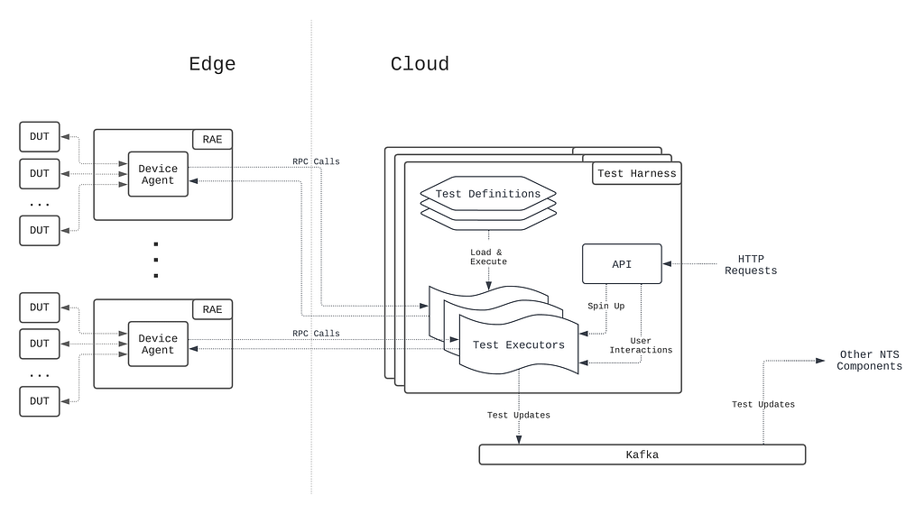
Test Target: In both the Netflix SDK and Partner testing use cases, the test targets are generally production devices, meaning they may not necessarily provide ssh / root access. As such, operations on devices by the automation system may only be reliably carried out through established device communication protocols such as DIAL or ADB, instead of through hardware-specific debugging tools that the Partners use.
Test Environment: The test targets are located both internally at Netflix and inside the Partner networks. To normalize the diversity of networking environments across both the Netflix and Partner networks and create a consistent and controllable computing environment on which users can run certification testing on their devices, Netflix provides a customized embedded computer to Partners called the Reference Automation Environment (RAE). The devices are in turn connected to the RAE, which provides access to the testing services provided by NTS.
Device Onboarding: Before a user can execute tests, they must make their device known to NTS and associate it with their Netflix Partner account in a process called device onboarding. The user achieves this by connecting the device to the RAE in a plug-and-play fashion. The RAE collects the device properties and publishes this information to NTS. The user then goes to the UI to claim the newly-visible device so that its ownership is associated with their account.
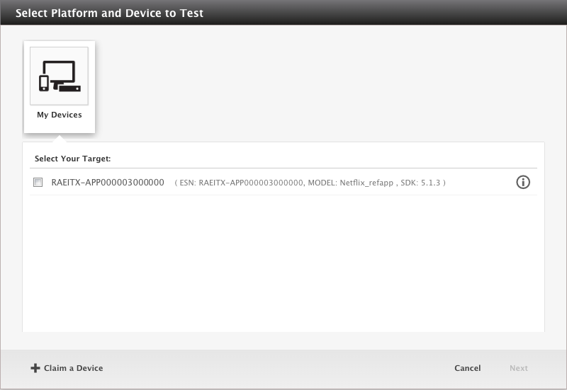
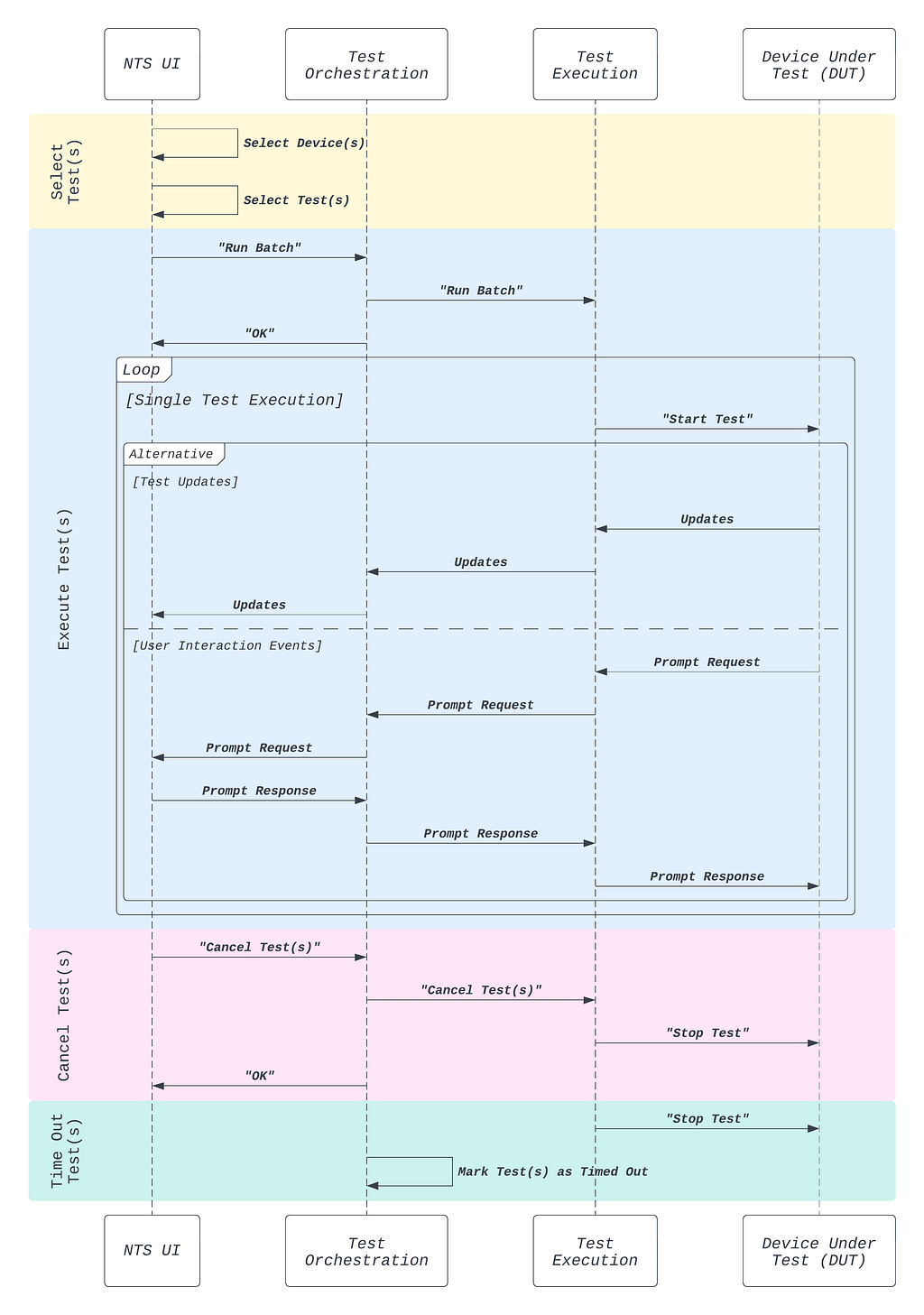
Device and Test Selection: To run tests, the user first selects from the browser-based web UI (the “NTS UI”) a target device from the list of devices under their ownership (Figure 1).
After a device has been selected, the user is presented with all tests that are applicable to the device being developed (Figure 2). The user then selects the subset of tests they are interested in running, and submits them for execution by NTS.

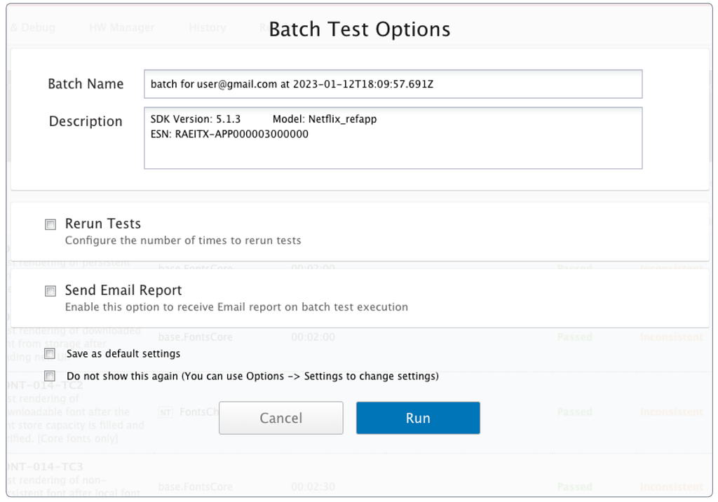
Tests can be executed as a single test run or as part of a batch run. In the latter case, additional execution options are available, such as the option to run multiple iterations of the same test or re-run tests on failure (Figure 3).
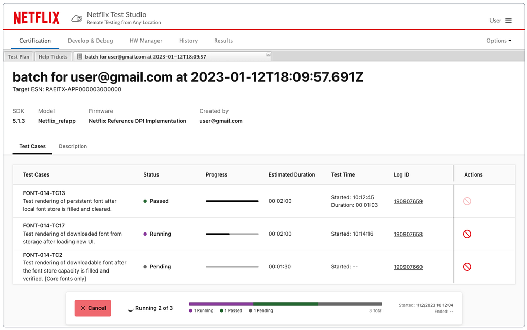
Test Execution: Once the tests are launched, the user will get a view of the tests being run, with a live update of their progress (Figure 4).
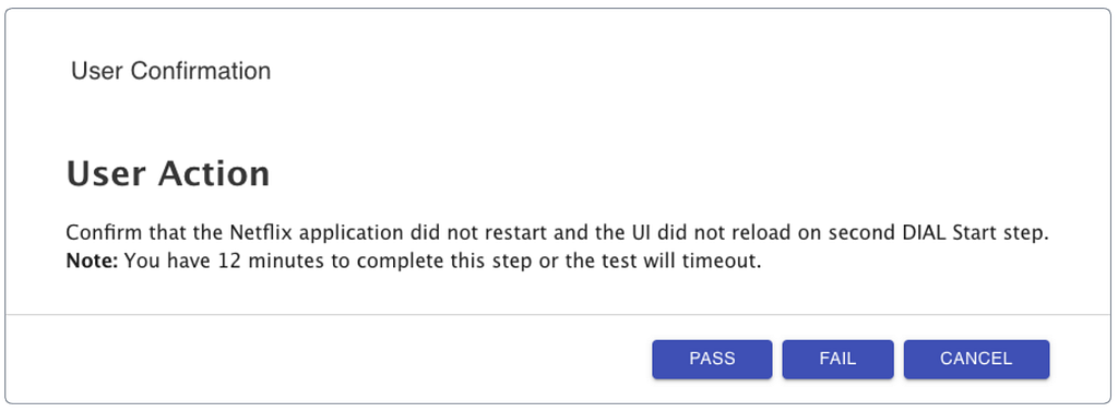
If the test is a manual test, prompts will appear in the UI at certain points during the test execution (Figure 5). The user follows the instructions in the prompt and clicks on the prompt buttons to notify the test to continue.
Defining the Stakeholders
To better define the business and system requirements for NTS, we must first identify who the stakeholders are and what their roles are in the business. For the purposes of this discussion, the major stakeholders in NTS are the following:
System Users: The system users are the Partners (system integrators) and the Partner Engineers that work with them. They select the certification targets, run tests, and analyze the results.
Test Authors: The test authors write the test cases that are to be run against the certification targets (devices). They are generally a subset of the system users, and are familiar or involved with the development of the Netflix SDK and UI.
System Developers: The system developers are responsible for developing the NTS platform and its components, adding new features, fixing bugs, maintaining uptime, and evolving the system architecture over time.
From the Use Cases to System Requirements
With the business workflows and stakeholders defined, we can articulate a set of high level system requirements / design guidelines that NTS should in theory follow:
Scheduling Non-requirement: The devices that are used in NTS form a pool of heterogeneous resources that have a diverse range of hardware constraints. However, NTS is built around the use case where users come in with a specific resource or pool of similar resources in mind and are searching for a subset of compatible tests to run on the target resource(s). This contrasts with test automation systems where users come in with a set of diverse tests, and are searching for compatible resources on which to run the tests. Resource sharing is possible, but it is expected to be manually coordinated between the users because the business workflows that use NTS often involve physical ownership of the device anyway. For these reasons, advanced resource scheduling is not a user requirement of this system.
Test Execution Component: Similar to other workflow automation systems, running tests in NTS involve performing tasks external to the target. These include controlling the target device, keeping track of the device state / connectivity, setting up test accounts for the test execution, collecting device logs, publishing test updates, validating test input parameters, and uploading test results, just to name a few. Thus, there needs to be a well-defined test execution stack that sits outside of the device under test to coordinate all these operations.
Proper State Management: Test execution statuses need to be accurately tracked, so that multiple users can follow what is happening while the test is running. Furthermore, certain tests require user interactions via prompts, which necessitate the system keeping track of messages being passed back and forth from the UI to the device. These two use cases call for a well-defined data model for representing test executions, as well as a system that provides consistent and reliable test execution state management.
Higher Level Execution Semantics: As noted from the business workflow description, users may want to run tests in batches, run multiple iterations of a test case, retry failing tests up to a given number of times, cancel tests in single or at the batch level, and be notified on the completion of a batch execution. Given that the execution of a single test case is already complex as is, these user features call for the need to encapsulate single test executions as the unit of abstraction that we can then use to define higher level execution semantics for supporting said features in a consistent manner.
Automated Supervision: Running tests on prototype hardware inherently comes with reliability issues, not to mention that it takes place in a network environment which we do not necessarily control. At any point during a test execution, the target device can run into any number of errors stemming from either the target device itself, the test execution stack, or the network environment. When this happens, the users should not be left without test execution updates and incomplete test results. As such, multiple levels of supervision need to be built into the test system, so that test executions are always cleaned up in a reliable manner.
Test Orchestration Component: The requirements for proper state management, higher level execution semantics, and automated supervision call for a well-defined test orchestration stack that handles these three aspects in a consistent manner. To clearly delineate the responsibilities of test orchestration from those of test execution, the test orchestration stack should be separate from and sit on top of the test execution component abstraction (Figure 6).
System Scalability: Scalability in NTS has different meaning for each of the system’s stakeholders. For the users, scalability implies the ability to always be able to run and interact with tests, no matter the scale (notwithstanding genuine device unavailability). For the test authors, scalability implies the ease of defining, extending, and debugging certification test cases. For the system developers, scalability implies the employment of distributed system design patterns and practices that scale up the development and maintenance velocities required to meet the needs of the users.
Adherence to the Paved Path: At Netflix, we emphasize building out solutions that use paved-path tooling as much as possible (see posts here and here). JVM and Kafka support are the most relevant components of the paved-path tooling for this article.
The Evolution of NTS
With the system requirements properly articulated, let us do a high-level walkthrough of the NTS 1.0 as implemented and examine some of its shortcomings with respect to meeting the requirements.
Test Execution Stack
In NTS 1.0, the test execution stack is partitioned into two components to address two orthogonal concerns: maintaining the test environment and running the actual tests. The RAE serves as the foundation for addressing the first concern. On the RAE sits the first component of the test execution stack, the device agent. The device agent is a monolithic daemon running on the RAE that manages the physical connections to the devices under test (DUTs), and provides an RPC API abstraction over physical device management and control.
Complementing the device agent is the test harness, which manages the actual test execution. The test harness accepts HTTP requests to run a single test case, upon which it will spin off a test executor instance to drive and manage the test case’s execution through RPC calls to the device agent managing the target device (see the NTS 1.0 blog post for details). Throughout the lifecycle of the test execution, the test harness publishes test updates to a message bus (Kafka in this case) that other services consume from.
Because the device agent provides a hardware abstraction layer for device control, the business logic for executing tests that resides in the test harness, from invoking device commands to publishing test results, is device-independent. This provides freedom for the component to be developed and deployed as a cloud-native application, so that it can enjoy the benefits of the cloud application model, e.g. write once run everywhere, automatic scalability, etc. Together, the device agent and the test harness form what is called the Hybrid Execution Context (HEC), i.e. the test execution is co-managed by a cloud and edge software stack (Figure 7).
Because the test harness contains all the common test execution business logic, it effectively acts as an “SDK” that device tests can be written on top of. Consequently, test case definitions are packaged as a common software library that the test harness imports on startup, and are executed as library methods called by the test executors in the test harness. This development model complements the write once run everywhere development model of test harness, since improvements to the test harness generally translate to test case execution improvements without any changes made to the test definitions themselves.
As noted earlier, executing a single test case against a device consists of many operations involved in the setup, runtime, and teardown of the test. Accordingly, the responsibility for each of the operations was divided between the device agent and test harness along device-specific and non-device-specific lines. While this seemed reasonable in theory, oftentimes there were operations that could not be clearly delegated to one or the other component. For example, since relevant logs are emitted by both software inside and outside of the device during a test, test log collection becomes a responsibility for both the device agent and test harness.
Presentation Layer
While the test harness publishes test events that eventually make their way into the test results store, the test executors and thus the intermediate test execution states are ephemeral and localized to the individual test harness instances that spun them. Consequently, a middleware service called the test dispatcher sits in between the users and the test harness to handle the complexity of test executor “discovery” (see the NTS 1.0 blog post for details). In addition to proxying test run requests coming from the users to the test harness, the test dispatcher most importantly serves materialized views of the intermediate test execution states to the users, by building them up through the ingestion of test events published by the test harness (Figure 8).

This presentation layer that is offered by the test dispatcher is more accurately described as a console abstraction to the test execution, since users rely on this service to not just follow the latest updates to a test execution, but also to interact with the tests that require user interaction. Consequently, bidirectionality is a requirement for the communications protocol shared between the test dispatcher service and the user interface, and as such, the WebSocket protocol was adopted due to its relative simplicity of implementation for both the test dispatcher and the user interface (web browsers in this case). When a test executes, users open a WebSocket session with the test dispatcher through the UI, and materialized test updates flow to the UI through this session as they are consumed by the service. Likewise, test prompt responses / cancellation requests flow from the UI back to the test dispatcher via the same session, and the test dispatcher forwards the message to the appropriate test executor instance in the test harness.
Batch Execution Stack
In NTS 1.0, the unit of abstraction for running tests is the single test case execution, and both the test execution stack and presentation layer was designed and implemented with this in mind. The construct of a batch run containing multiple tests was introduced only later in the evolution of NTS, being motivated by a set of related user-demanded features: the ability to run and associate multiple tests together, the ability to retry tests on failure, and the ability to be notified when a group of tests completes. To address the business logic of managing batch runs, a batch executor was developed, separate from both the test harness and dispatcher services (Figure 9).

Similar to the test dispatcher service, the batch execution service proxies batch run requests coming from the users, and is ultimately responsible for dispatching the individual test runs in the batch through the test harness. However, the batch execution service maintains its own data model of the test execution that is separate from and thus incompatible with that materialized by the test dispatcher service. This is a necessary difference considering the unit of abstraction for running tests using the batch execution service is the batch run.
Examining the Shortcomings of NTS 1.0
Having described the major system components at a high level, we can now analyze some of the shortcomings of the system in detail:
Inconsistent Execution Semantics: Because batch runs were introduced as an afterthought, the semantics of batch executions in relation to those of the individual test executions were never fully clarified in implementation. In addition, the presence of both the test dispatcher and batch executor created a bifurcation in test executions management, where neither service alone satisfied the users’ needs. For example, a single test that is kicked off as part of a batch run through the batch executor must be canceled through the test dispatcher service. However, cancellation is only possible if the test is in a running state, since the test dispatcher has no information about tests prior to their execution. Behaviors such as this often resulted in the system appearing inconsistent and unintuitive to the users, while presenting a knowledge overhead for the system developers.
Test Execution Scalability and Reliability: The test execution stack suffered two technical issues that hampered its reliability and ability to scale. The first is in the partitioning of the test execution stack into two distinct components. While this division had emerged naturally from the setup of the business workflow, the device agent and test harness are fundamentally two pieces of a common stack separated by a control plane, i.e. the network. The conditions of the network at the Partner sites are known to be inconsistent and sometimes unreliable, as there might be traffic congestion, low bandwith, or unique firewall rules in place. Furthermore, RPC communications between the device agent and test harness are not direct, but go through a few more system components (e.g. gateway services). For these reasons, test executions in practice often suffer from a host of stability, reliability, and latency issues, most of which we cannot take action upon.
The second technical issue is in the implementation of the test executors hosted by the test harness. When a test case is run, a full thread is spawned off to manage its execution, and all intermediate test execution state is stored in thread-local memory. Given that much of the test execution lifecycle is involved with making blocking RPC calls, this choice of implementation in practice limits the number of tests that can effectively be run and managed per test harness instance. Moreover, the decision to maintain intermediate test execution state only in thread-local memory renders the test harness fragile, as all test executors running on a given test harness instance will be lost along with their data if the instance goes down. Operational issues stemming from the brittle implementation of the test executors and from the partitioning of the test execution stack frequently exacerbate each other, leading to situations where test executions are slow, unreliable, and prone to infrastructure errors.
Presentation Layer Scalability: In theory, the dispatcher service’s WebSocket server can scale up user sessions to the maximum number of HTTP connections allowed by the service and host configuration. However, the service was designed to be stateless so as to reduce the codebase size and complexity. This meant that the dispatcher service had to initialize a new Kafka consumer, read from the beginning of the target partition, filter for the relevant test updates, and build the intermediate test execution state on the fly each time a user opened a new WebSocket session with the service. This was a slow and resource-intensive process, which limited the scalability of the dispatcher service as an interactive test execution console for users in practice.
Test Authoring Scalability: Because the common test execution business logic was bundled with the test harness as a de facto SDK, test authors had to actually be familiar with the test harness stack in order to define new test cases. For the test authors, this presented a huge learning curve, since they had to learn a large codebase written in a programming language and toolchain that was completely different from those used in Netflix SDK and UI. Since only the test harness maintainers can effectively contribute test case definitions and improvements, this became a bottleneck as far as development velocity was concerned.
Unreliable State Management: Each of the three core services has a different policy with respect to test execution state management. In the test harness, state is held in thread-local memory, while in the test dispatcher, it is built on the fly by reading from Kafka with each new console session. In the batch executor, on the other hand, intermediate test execution states are ignored entirely and only test results are stored. Because there is no persistence story with regards to intermediate test execution state, and because there is no data model to represent test execution states consistently across the three services, it becomes very difficult to coordinate and track test executions. For example, two WebSocket sessions to the same test execution are generally not reproducible if user interactions such as prompt responses are involved, since each session has its own materialization of the test execution state. Without the ability to properly model and track test executions, supervision of test executions is consequently non-existent.
Moving To an Intentional Architecture
The evolution of NTS can best be described as that of an emergent system architecture, with many features added over time to fulfill the users’ ever-increasing needs. It became apparent that this model brought forth various shortcomings that prevented it from satisfying the system requirements laid out earlier. We now discuss the high-level architectural changes we have made with NTS 2.0, which was built with an intentional design approach to address the system requirements of the business problem.
Decoupling Test Definitions
In NTS 2.0, tests are defined as scripts against the Netflix SDK that execute on the device itself, as opposed to library code that is dependent on and executes in the test harness. These test definitions are hosted on a separate service where they can be accessed by the Netflix SDK on devices located in the Partner networks (Figure 10).

This change brings several distinct benefits to the system. The first is that the new setup is more aligned with device certification, where ultimately we are testing the integration of the Netflix SDK with the target device’s firmware. The second is that we are able to consolidate instrumentation and logging onto a single stack, which simplifies the debugging process for the developers. In addition, by having tests be defined using the same programming language and toolchain used to develop the Netflix UI, the learning curve for writing and maintaining tests is significantly reduced for the test authors. Finally, this setup strongly decouples test definitions from the rest of the test execution infrastructure, allowing for the two to be developed separately in parallel with improved velocity.
Defining the Job Execution Model
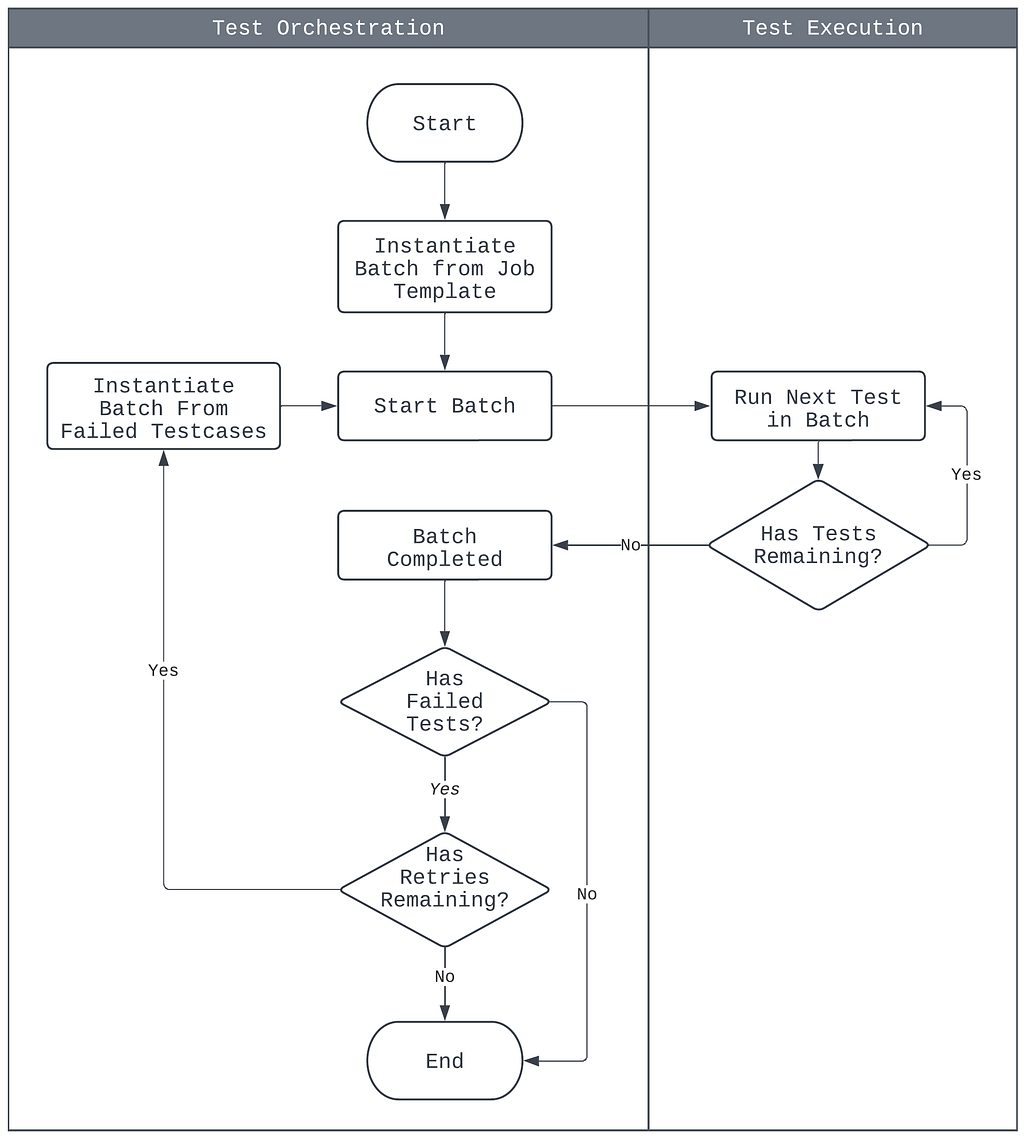
A proper job execution model with concise semantics has been defined in NTS 2.0 to address the inconsistent semantics between single test and batch executions (Figure 11). The model is summarized as follows:
- The base unit of test execution is the batch. A batch consists of one or more test cases to be run sequentially on the target device.
- The base unit of test orchestration is the job. A job is a template containing a list of test cases to be run, configurations for test retries and job notifications, and information on the target device.
- All test run requests create a job template, from which batches are instantiated for execution. This includes single test run requests.
- Upon batch completion, a new batch may be instantiated from the source job, but containing only the subset of the test cases that failed earlier. Whether or not this occurs depends on the source job’s test retries configuration.
- A job is considered finished when its instantiated batches and subsequent retries have completed. Notifications may then be sent out according to the job’s configuration.
- Cancellations are applicable to either the single test execution level or the batch execution level. Jobs are considered canceled when its current batch instantiation is canceled.
The newly-defined job execution model thoroughly clarifies the semantics of single test and batch executions while remaining consistent with all existing use cases of the system, and has informed the re-architecting of both the test execution and orchestration components, which we will discuss in the next few sections.
Replacement of the Control Plane
In NTS 1.0, the device agent at the edge and the test harness in the cloud communicate to each other via RPC calls proxied by intermediate gateway services. As noted in great detail earlier, this setup brought many stability, reliability, and latency issues that were observed in test executions. With NTS 2.0, this point-to-point-based control plane is replaced with a message bus-based control plane that is built on MQTT and Kafka (Figure 12).
MQTT is an OASIS standard messaging protocol for the Internet of Things (IoT) and was designed as a highly lightweight yet reliable publish/subscribe messaging transport that is ideal for connecting remote devices with a small code footprint and minimal network bandwidth. MQTT clients connect to the MQTT broker and send messages prefixed with a topic. The broker is responsible for receiving all messages, filtering them, determining who is subscribed to which topic, and sending the messages to the subscribed clients accordingly. The key features that make MQTT highly appealing to us are its support for request retries, fault tolerance, hierarchical topics, client authentication and authorization, per-topic ACLs, and bi-directional request/response message patterns, all of which are crucial for the business use cases around NTS.
Since the paved-path solution at Netflix supports Kafka, a bridge is established between the two protocols to allow cloud-side services to communicate with the control plane (Figure 12). Through the bridge, MQTT messages are converted directly to Kafka records, where the record key is set to be the MQTT topic that the message was assigned to. We take advantage of this construction by having test execution updates published on MQTT contain the test_id in the topic. This forces all updates for a given test execution to effectively appear on the same Kafka partition with a well-defined message order for consumption by NTS component cloud services.
The introduction of the new control plane has enabled communications between different NTS components to be carried out in a consistent, scalable, and reliable manner, regardless of where the components were located. One example of its use is described in our earlier blog post about reliable devices management. The new control plane sets the foundations for the evolution of the test execution stack in NTS 2.0, which we discuss next.
Migration from a Hybrid to Local Execution Context
The test execution component is completely migrated over from the cloud to the edge in NTS 2.0. This includes functionality from the batch execution stack in NTS 1.0, since batch executions are the new base unit of test execution. The migration immediately addresses the long standing problems of network reliability and latency in test executions, since the entire test execution stack now sits together in the same isolated environment, the RAE, instead of being partitioned by a control plane.

During the migration, the test harness and the device agent components were modularized, as each aspect of test execution management — device state management, device communications protocol management, batch executions management, log collection, etc — was moved into a dedicated system service running on the RAE that communicated with the other components via the new control plane (Figure 12). Together with the new control plane, these new local modules form what is called the Local Execution Context (LEC). By consolidating test execution management onto the edge and thus in close proximity to the device, the LEC becomes largely immune from the many network-related scalability, reliability, and stability issues that the HEC model frequently encounters. Alongside with the decoupling of test definitions from the test harness, the LEC has significantly reduced the complexity of the test execution stack, and has paved the way for its development to be parallelized and thus scalable.
Proper State Modeling with Event Sourcing
Test orchestration covers many aspects: support for the established job execution model (kicking off and running jobs), consistent state management for test executions, reconciliation of user interaction events with test execution state, and overall job execution supervision. These functions were divided amongst the three core services in NTS 1.0, but without a consistent model of the intermediate execution states that they can rely upon for coordination, test orchestration as defined by the system requirements could not be reliably achieved. With NTS 2.0, a unified data schema for test execution updates is defined according to the job execution model, with the data itself persisted in storage as an append-only log. In this state management model, all updates for a given test execution, including user interaction events, are stored as a totally-ordered sequence of immutable records ordered by time and grouped by the test_id. The append-only property here is a very powerful feature, because it gives us the ability to materialize a test execution state at any intermediate point in time simply by replaying the append-only log for the test execution from the beginning up until the given timestamp. Because the records are immutable, state materializations are always fully reproducible.
Since the test execution stack continuously publishes test updates to the control plane, state management at the test orchestration layer simply becomes a matter of ingesting and storing these updates in the correct order in accordance with the Event Sourcing Pattern. For this, we turn to the solution provided by Alpakka-Kafka, whose adoption we have previously pioneered in the implementation of our devices management platform (Figure 13). To summarize here, we chose Alpakka-Kafka as the basis of the test updates ingestion infrastructure because it fulfilled the following technical requirements: support for per-partition in-order processing of events, back-pressure support, fault tolerance, integration with the paved-path tooling, and long-term maintainability. Ingested updates are subsequently persisted into a log store backed by CockroachDB. CockroachDB was chosen as the backing store because it is designed to be horizontally scalable and it offers the SQL capabilities needed for working with the job execution data model.

With proper event sourcing in place and the test execution stack fully migrated over to the LEC, the remaining functionality in the three core services is consolidated into dedicated single service in NTS 2.0, effectively replacing and improving upon the former three in all areas where test orchestration was concerned. The scalable state management solution provided by this test orchestration service becomes the foundation for scalable presentation and job supervision in NTS 2.0, which we discuss next.
Scaling Up the Presentation Layer
The new test orchestration service serves the presentation layer, which, as with NTS 1.0, provides a test execution console abstraction implemented using WebSocket sessions. However, for the console abstraction to be truly reliable and functional, it needs to fulfill several requirements. The first and foremost is that console sessions must be fully reproducible, i.e. two users interacting with the same test execution should observe the exact same behavior. This was an area that was particularly problematic in NTS 1.0. The second is that console sessions must scale up with the number of concurrent users in practice, i.e. sessions should not be resource-intensive. The third is that communications between the session console and the user should be minimal and efficient, i.e. new test execution updates should be delivered to the user only once. This requirement implies the need for maintaining session-local memory to keep track of delivered updates. Finally, the test orchestration service itself needs to be able to intervene in console sessions, e.g. send session liveness updates to the users on an interval schedule or notify the users of session termination if the service instance hosting the session is shutting down.
To handle all of these requirements in a consistent yet scalable manner, we turn to the Actor Model for inspiration. The Actor Model is a concurrency model in which actors are the universal primitive of concurrent computation. Actors send messages to each other, and in response to incoming messages, they can perform operations, create more actors, send out other messages, and change their future behavior. Actors also maintain and modify their own private state, but they can only affect each other’s states indirectly through messaging. In-depth discussions of the Actor Model and its many applications can be found here and here.

The Actor Model naturally fits the mental model of the test execution console, since the console is fundamentally a standalone entity that reacts to messages (e.g. test updates, service-level notifications, and user interaction events) and maintains internal state. Accordingly, we modeled test execution sessions as such using Akka Typed, a well-known and highly-maintained actor system implementation for the JVM (Figure 14). Console sessions are instantiated when a WebSocket connection is opened by the user to the service, and upon launch, the console begins fetching new test updates for the given test_id from the data store. Updates are delivered to the user over the WebSocket connection and saved to session-local memory as record to keep track of what has already been delivered, while user interaction events are forwarded back to the LEC via the control plane. The polling process is repeated on a cron schedule (every 2 seconds) that is registered to the actor system’s scheduler during console instantiation, and the polling’s data query pattern is designed to be aligned with the service’s state management model.
Putting in Job Supervision
As a distributed system whose components communicate asynchronously and are involved with prototype embedded devices, faults frequently occur throughout the NTS stack. These faults range from device loops and crashes to the RAE being temporarily disconnected from the network, and generally result in missing test updates and/or incomplete test results if left unchecked. Such undefined behavior is a frequent occurrence in NTS 1.0 that impedes the reliability of the presentation layer as an accurate view of test executions. In NTS 2.0, multiple levels of supervision are present across the system to address this class of issues. Supervision is carried out through checks that are scheduled throughout the job execution lifecycle in reaction to the job’s progress. These checks include:
- Handling response timeouts for requests sent from the test orchestration service to the LEC.
- Handling test “liveness”, i.e. ensuring that updates are continuously present until the test execution reaches a terminal state.
- Handling test execution timeouts.
- Handling batch execution timeouts.
When these faults occur, the checks will discover them and automatically clean up the faulting test execution, e.g. marking test results as invalid, releasing the target device from reservation, etc. While some checks exist in the LEC stack, job-level supervision facilities mainly reside in the test orchestration service, whose log store can be reliably used for monitoring test execution runs.
Discussion
System Behavioral Reliability
The importance of understanding the business problem space and cementing this understanding through proper conceptual modeling cannot be underscored enough. Many of the perceived reliability issues in NTS 1.0 can be attributed to undefined behavior or missing features. These are an inevitable occurrence in the absence of conceptual modeling and thus strongly codified expectations of system behavior. With NTS 2.0, we properly defined from the very beginning the job execution model, the data schema for test execution updates according to the model, and the state management model for test execution states (i.e. the append-only log model). We then implemented various system-level features that are built upon these formalisms, such as event-sourcing of test updates, reproducible test execution console sessions, and job supervision. It is this development approach, along with the implementation choices made along the way, that empowers us to achieve behavioral reliability across the NTS system in accordance with the business requirements.
System Scalability
We can examine how each component in NTS 2.0 addresses the scalability issues that are present in its predecessor:
LEC Stack: With the consolidation of the test execution stack fully onto the RAE, the challenge of scaling up test executions is now broken down into two separate problems:
- Whether or not the LEC stack can support executing as many tests simultaneously as the maximum number of devices that can be connected to the RAE.
- Whether or not the communications between the edge and the cloud can scale with the number of RAEs in the system.
The first problem is naturally resolved by hardware-imposed limitations on the number of connected devices, as the RAE is an embedded appliance. The second refers to the scalability of the NTS control plane, which we will discuss next.
Control Plane: With the replacement of the point-to-point RPC-based control plane with a message bus-based control plane, system faults stemming from Partner networks have become a rare occurrence and RAE-edge communications have become scalable. For the MQTT side of the control plane, we used HiveMQ as the cloud MQTT broker. We chose HiveMQ because it met all of our business use case requirements in terms of performance and stability (see our adoption report for details), and came with the MQTT-Kafka bridging support that we needed.
Event Sourcing Infrastructure: The event-sourcing solution provided by Alpakka-Kafka and CockroachDB has already been demonstrated to be very performant, scalable, and fault tolerant in our earlier work on reliable devices management.
Presentation Layer: The current implementation of the test execution console abstraction using actors removed the practical scaling limits of the previous implementation. The real advantage of this implementation model is that we can achieve meaningful concurrency and performance without having to worry about the low-level details of thread pool management and lock-based synchronization. Notably, systems built on Akka Typed have been shown to support roughly 2.5 million actors per GB of heap and relay actor messages at a throughput of nearly 50 million messages per second.
To be thorough, we performed basic load tests on the presentation layer using the Gatling load-testing framework to verify its scalability. The simulated test scenario per request is as follows:
- Open a test execution console session (i.e. WebSocket connection) in the test orchestration service.
- Wait for 2 to 3 minutes (randomized), during which the session will be polling the data store at 2 second intervals for test updates.
- Close the session.
This scenario is comparable to the typical NTS user workflow that involves the presentation layer. The load test plan is as follows:
- Burst ramp-up requests to 1000 over 5 seconds.
- Add 80 new requests per second for 10 minutes.
- Wait for all requests to complete.
We observed that, in load tests of a single client machine (2.4 GHz, 8-Core, 32 GB RAM) running against a small cluster of 3 AWS m4.xlarge instances, we were able to peg the client at over 10,900 simultaneous live WebSocket connections before the client’s limits were reached (Figure 15). On the server side, neither CPU nor memory utilization appeared significantly impacted for the duration of the tests, and the database connection pool was able to handle the query load from all the data store polling (Figures 16–18). We can conclude from these load test results that scalability of the presentation layer has been achieved with the new implementation.
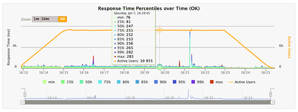


Job Supervision: While the actual business logic may be complex, job supervision itself is a very lightweight process, as checks are reactively scheduled in response to events across the job execution cycle. In implementation, checks are scheduled through the Akka scheduler and run using actors, which have been shown above to scale very well.
Development Velocity
The design decisions we have made with NTS 2.0 have simplified the NTS architecture and in the process made the platform run tests observably much faster, as there are simply a lot less moving components to work with. Whereas it used to take roughly 60 seconds to run through a “Hello, World” device test from setup to teardown, now it takes less than 5 seconds. This has translated to increased development velocity for our users, who can now iterate their test authoring and device integration / certification work much more frequently.
In NTS 2.0, we have thoroughly added multiple levels of observability across the stack using paved-path tools, from contextual logging to metrics to distributed tracing. Some of these capabilities were previously not available in NTS 1.0 because the component services were built prior to the introduction of paved-path tooling at Netflix. Combined with the simplification of the NTS architecture, this has increased development velocity for the system maintainers by an order of magnitude, as user-reported issues in general can now be tracked down and fixed within the same day as they were reported, for example.
Costs Reduction
Though our discussion of NTS 1.0 focused on the three core services, in reality there are many auxiliary services in between that coordinate different aspects of a test execution, such as RPC requests proxying from cloud to edge, test results collection, etc. Over the course of building NTS 2.0, we have deprecated a total of 10 microservices whose roles have been either obsolesced by the new architecture or consolidated into the LEC and test orchestration service. In addition, our work has paved the way for the eventual deprecation of 5 additional services and the evolution of several others. The consolidation of component services along with the increase in development and maintenance velocity brought about by NTS 2.0 has significantly reduced the business costs of maintaining the NTS platform, in terms of both compute and developer resources.
Conclusion
Systems design is a process of discovery and can be difficult to get right on the first iteration. Many design decisions need to be considered in light of the business requirements, which evolve over time. In addition, design decisions must be regularly revisited and guided by implementation experience and customer feedback in a process of value-driven development, while avoiding the pitfalls of an emergent model of system evolution. Our in-field experience with NTS 1.0 has thoroughly informed the evolution of NTS into a device testing solution that better satisfies the business workflows and requirements we have while scaling up developer productivity in building out and maintaining this solution.
Though we have brought in large changes with NTS 2.0 that addressed the systemic shortcomings of its predecessor, the improvements discussed here are focused on only a few components of the overall NTS platform. We have previously discussed reliable devices management, which is another large focus domain. The overall reliability of the NTS platform rests on significant work made in many other key areas, including devices onboarding, the MQTT-Kafka transport, authentication and authorization, test results management, and system observability, which we plan to discuss in detail in future blog posts. In the meantime, thanks to this work, we expect NTS to continue to scale with increasing workloads and diversity of workflows over time according to the needs of our stakeholders.
![]()
NTS: Reliable Device Testing at Scale was originally published in Netflix TechBlog on Medium, where people are continuing the conversation by highlighting and responding to this story.
Ultimate UST Projector Screen Comparison – 8 CLR/ALR Screens Tested and Reviewed
Post Syndicated from The Hook Up original https://www.youtube.com/watch?v=2b8PXZtL1q8
Lenovo ThinkStation PX Dual SPR and the Xeon W Duo P7 and P5 Launched
Post Syndicated from Cliff Robinson original https://www.servethehome.com/lenovo-thinkstation-px-dual-spr-and-the-xeon-w-duo-p7-and-p5-launched/
The Lenovo ThinkStation PX workstation houses dual 4th Gen Intel Xeon processors while the P7 uses a Xeon W-3400 and the P5 has a Xeon W-2400
The post Lenovo ThinkStation PX Dual SPR and the Xeon W Duo P7 and P5 Launched appeared first on ServeTheHome.
Establishing a data perimeter on AWS: Allow only trusted resources from my organization
Post Syndicated from Laura Reith original https://aws.amazon.com/blogs/security/establishing-a-data-perimeter-on-aws-allow-only-trusted-resources-from-my-organization/
Companies that store and process data on Amazon Web Services (AWS) want to prevent transfers of that data to or from locations outside of their company’s control. This is to support security strategies, such as data loss prevention, or to comply with the terms and conditions set forth by various regulatory and privacy agreements. On AWS, a resource perimeter is a set of AWS Identity and Access Management (IAM) features and capabilities that you can use to build your defense-in-depth protection against unintended data transfers. In this third blog post of the Establishing a data perimeter on AWS series, we review the benefits and implementation considerations when you define your resource perimeter.
The resource perimeter is one of the three perimeters in the data perimeter framework on AWS and has the following two control objectives:
- My identities can access only trusted resources – This helps to ensure that IAM principals that belong to your AWS Organizations organization can access only the resources that you trust.
- Only trusted resources can be accessed from my network – This helps to ensure that only resources that you trust can be accessed through expected networks, regardless of the principal that is making the API call.
Trusted resources are the AWS resources, such as Amazon Simple Storage Service (Amazon S3) buckets and objects or Amazon Simple Notification Service (Amazon SNS) topics, that are owned by your organization and in which you store and process your data. Additionally, there are resources outside your organization that your identities or AWS services acting on your behalf might need to access. You will need to consider these access patterns when you define your resource perimeter.
Security risks addressed by the resource perimeter
The resource perimeter helps address three main security risks.
Unintended data disclosure through use of corporate credentials — Your developers might have a personal AWS account that is not part of your organization. In that account, they could configure a resource with a resource-based policy that allows their corporate credentials to interact with the resource. For example, they could write an S3 bucket policy that allows them to upload objects by using their corporate credentials. This could allow the intentional or unintentional transfer of data from your corporate environment — your on-premises network or virtual private cloud (VPC) — to their personal account. While you advance through your least privilege journey, you should make sure that access to untrusted resources is prohibited, regardless of the permissions granted by identity-based policies that are attached to your IAM principals. Figure 1 illustrates an unintended access pattern where your employee uses an identity from your organization to move data from your on-premises or AWS environment to an S3 bucket in a non-corporate AWS account.
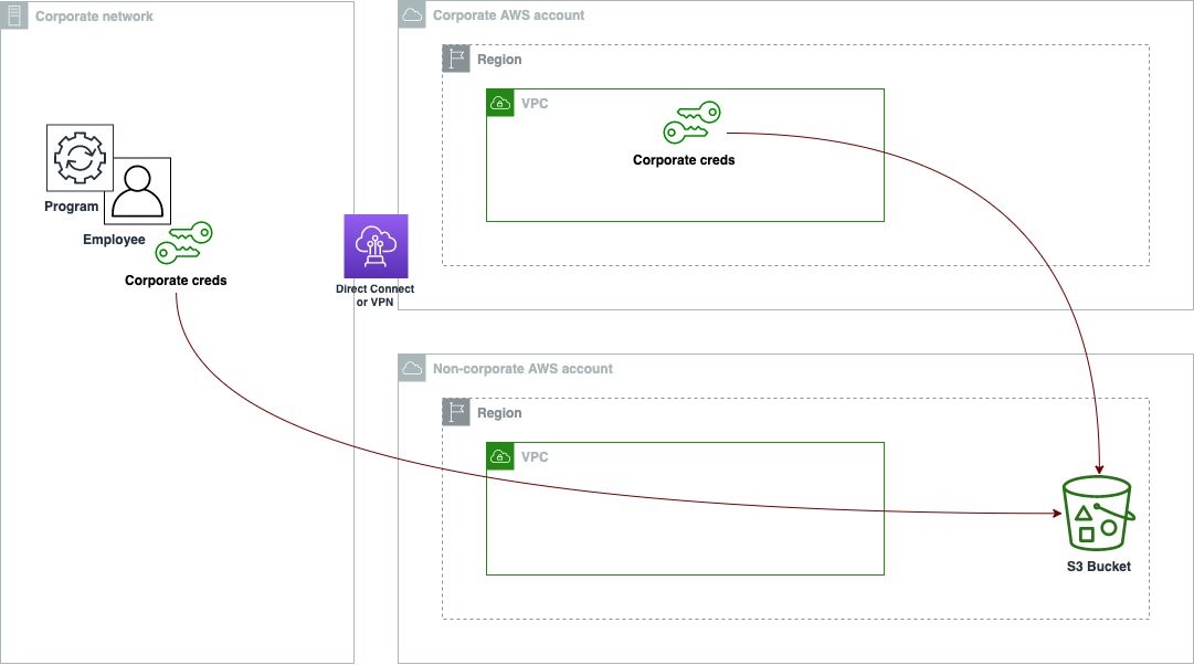
Figure 1: Unintended data transfer to an S3 bucket outside of your organization by your identities
Unintended data disclosure through non-corporate credentials usage — There is a risk that developers could introduce personal IAM credentials to your corporate network and attempt to move company data to personal AWS resources. We discussed this security risk in a previous blog post: Establishing a data perimeter on AWS: Allow only trusted identities to access company data. In that post, we described how to use the aws:PrincipalOrgID condition key to prevent the use of non-corporate credentials to move data into an untrusted location. In the current post, we will show you how to implement resource perimeter controls as a defense-in-depth approach to mitigate this risk.
Unintended data infiltration — There are situations where your developers might start the solution development process using commercial datasets, tooling, or software and decide to copy them from repositories, such as those hosted on public S3 buckets. This could introduce malicious components into your corporate environment, your on-premises network, or VPCs. Establishing the resource perimeter to only allow access to trusted resources from your network can help mitigate this risk. Figure 2 illustrates the access pattern where an employee with corporate credentials downloads assets from an S3 bucket outside of your organization.

Figure 2: Unintended data infiltration
Implement the resource perimeter
To achieve the resource perimeter control objectives, you can implement guardrails in your AWS environment by using the following AWS policy types:
- Service control policies (SCPs) – Organization policies that are used to centrally manage and set the maximum available permissions for your IAM principals. SCPs help you ensure that your accounts stay within your organization’s access control guidelines. In the context of the resource perimeter, you will use SCPs to help prevent access to untrusted resources from AWS principals that belong to your organization.
- VPC endpoint policy – An IAM resource-based policy that is attached to a VPC endpoint to control which principals, actions, and resources can be accessed through a VPC endpoint. In the context of the resource perimeter, VPC endpoint policies are used to validate that the resource the principal is trying to access belongs to your organization.
The condition key used to constrain access to resources in your organization is aws:ResourceOrgID. You can set this key in an SCP or VPC endpoint policy. The following table summarizes the relationship between the control objectives and the AWS capabilities used to implement the resource perimeter.
| Control objective | Implemented by using | Primary IAM capability |
| My identities can access only trusted resources | SCPs | aws:ResourceOrgID |
| Only trusted resources can be accessed from my network | VPC endpoint policies | aws:ResourceOrgID |
In the next section, you will learn how to use the IAM capabilities listed in the preceding table to implement each control objective of the resource perimeter.
My identities can access only trusted resources
The following is an example of an SCP that limits all actions to only the resources that belong to your organization. Replace <MY-ORG-ID> with your information.
In this policy, notice the use of the negated condition key StringNotEqualsIfExists. This means that this condition will evaluate to true and the policy will deny API calls if the organization identifier of the resource that is being accessed differs from the one specified in the policy. It also means that this policy will deny API calls if the resource being accessed belongs to a standalone account, which isn’t part of an organization. The negated condition operators in the Deny statement mean that the condition still evaluates to true if the key is not present in the request; however, as a best practice, I added IfExists to the end of the StringNotEquals operator to clearly express the intent in the policy.
Note that for a permission to be allowed for a specific account, a statement that allows access must exist at every level of the hierarchy of your organization.
Only trusted resources can be accessed from my network
You can achieve this objective by combining the SCP we just reviewed with the use of aws:PrincipalOrgID in your VPC endpoint policies, as shown in the Establishing a data perimeter on AWS: Allow only trusted identities to access company data blog post. However, as a defense in depth, you can also apply resource perimeter controls on your networks by using aws:ResourceOrgID in your VPC endpoint policies.
The following is an example of a VPC endpoint policy that allows access to all actions but limits access to only trusted resources and identities that belong to your organization. Replace <MY-ORG-ID> with your information.
The preceding VPC endpoint policy uses the StringEquals condition operator. To invoke the Allow effect, the principal making the API call and the resource they are trying to access both need to belong to your organization. Compared to the SCP example that we reviewed earlier, your intent for this policy is different — you want to make sure that the Allow condition evaluates to true only if the specified key exists in the request. Additionally, VPC endpoint policies apply to principals, as long as their request flows through the VPC endpoint.
In VPC endpoint policies, you do not grant permissions; rather, you define the maximum allowed access through the network. Therefore, this policy uses an Allow effect.
Extend your resource perimeter
The previous two policies help you ensure that your identities and networks can only be used to access AWS resources that belong to your organization. However, your company might require that you extend your resource perimeter to also include AWS owned resources — resources that do not belong to your organization and that are accessed by your principals or by AWS services acting on your behalf. For example, if you use the AWS Service Catalog in your environment, the service creates and uses Amazon S3 buckets that are owned by the service to store products. To allow your developers to successfully provision AWS Service Catalog products, your resource perimeter needs to account for this access pattern. The following statement shows how to account for the service catalog access pattern. Replace <MY-ORG-ID> with your information.
Note that the EnforceResourcePerimeter statement in the SCP was modified to exclude s3:GetObject, s3:PutObject, and s3:PutObjectAcl actions from its effect (NotAction element). This is because these actions are performed by the Service Catalog to access service-owned S3 buckets. These actions are then restricted in the ExtendResourcePerimeter statement, which includes two negated condition keys. The second statement denies the previously mentioned S3 actions unless the resource that is being accessed belongs to your organization (StringNotEqualsIfExists with aws:ResourceOrgID), or the actions are performed by Service Catalog on your behalf (ForAllValues:StringNotEquals with aws:CalledVia). The aws:CalledVia condition key compares the services specified in the policy with the services that made requests on behalf of the IAM principal by using that principal’s credentials. In the case of the Service Catalog, the credentials of a principal who launches a product are used to access S3 buckets that are owned by the Service Catalog.
It is important to highlight that we are purposely not using the aws:ViaAWSService condition key in the preceding policy. This is because when you extend your resource perimeter, we recommend that you restrict access to only calls to buckets that are accessed by the service you are using.
You might also need to extend your resource perimeter to include the third-party resources of your partners. For example, you could be working with business partners that require your principals to upload or download data to or from S3 buckets that belong to their account. In this case, you can use the aws:ResourceAccount condition key in your resource perimeter policy to specify resources that belong to the trusted third-party account.
The following is an example of an SCP that accounts for access to the Service Catalog and third-party partner resources. Replace <MY-ORG-ID> and <THIRD-PARTY-ACCOUNT> with your information.
To account for access to trusted third-party account resources, the condition StringNotEqualsIfExists in the ExtendResourcePerimeter statement now also contains the condition key aws:ResourceAccount. Now, the second statement denies the previously mentioned S3 actions unless the resource that is being accessed belongs to your organization (StringNotEqualsIfExists with aws:ResourceOrgID), to a trusted third-party account (StringNotEqualsIfExists with aws:ResourceAccount), or the actions are performed by Service Catalog on your behalf (ForAllValues:StringNotEquals with aws:CalledVia).
The next policy example demonstrates how to extend your resource perimeter to permit access to resources that are owned by your trusted third parties through the networks that you control. This is required if applications running in your VPC or on-premises need to be able to access a dataset that is created and maintained in your business partner AWS account. Similar to the SCP example, you can use the aws:ResourceAccount condition key in your VPC endpoint policy to account for this access pattern. Replace <MY-ORG-ID>, <THIRD-PARTY-ACCOUNT>, and <THIRD-PARTY-RESOURCE-ARN> with your information.
The second statement, AllowRequestsByOrgsIdentitiesToThirdPartyResources, in the updated VPC endpoint policy allows s3:GetObject, s3:PutObject, and s3:PutObjectAcl actions on trusted third-party resources (StringEquals with aws:ResourceAccount) by principals that belong to your organization (StringEquals with aws:PrincipalOrgID).
Note that you do not need to modify your VPC endpoint policy to support the previously discussed Service Catalog operations. This is because calls to Amazon S3 made by Service Catalog on your behalf originate from the Service Catalog service network and do not traverse your VPC endpoint. However, you should consider access patterns that are similar to the Service Catalog example when defining your trusted resources. To learn about services with similar access patterns, see the IAM policy samples section later in this post.
Deploy the resource perimeter at scale
For recommendations on deploying a data perimeter at scale, see the Establishing a data perimeter on AWS: Allow only trusted identities to access company data blog post. The section titled Deploying the identity perimeter at scale provides the details on how to achieve this for your organization.
IAM policy samples
Our GitHub repository contains policy examples that illustrate how to implement perimeter controls for a variety of AWS services. The policy examples in the repository are for reference only. You will need to tailor them to suit the specific needs of your AWS environment.
Conclusion
In this blog post, you learned about the resource perimeter, the control objectives achieved by the perimeter, and how to write SCPs and VPC endpoint policies that help achieve these objectives for your organization. You also learned how to extend your perimeter to include AWS service-owned resources and your third-party partner-owned resources.
For additional learning opportunities, see the Data perimeters on AWS page. This information resource provides additional materials such as a data perimeter workshop, blog posts, whitepapers, and webinar sessions.
If you have questions, comments, or concerns, contact AWS Support or browse AWS re:Post. If you have feedback about this post, submit comments in the Comments section below.
Want more AWS Security news? Follow us on Twitter.
How GitHub Docs’ new search works
Post Syndicated from Peter Bengtsson original https://github.blog/2023-03-09-how-github-docs-new-search-works/
Until recently, the site-search on GitHub Docs was an in-memory solution. While it was a great starting point, we ultimately needed a solution that would scale with our growing needs, so we rewrote it in Elasticsearch. In this blog post, we share how the implementation works and how you can impress users with your site-search by doing the same.
How it started
Our previous solution couldn’t scale because it required loading all of the records into memory (the Node.js code that Express.js runs). This means that we’d need to scrape all the searchable text—title, headings, breadcrumbs, content, etc.—and store that data somewhere so it could quickly be loaded in the Node process runtime. To store the data, we used the Git repository itself, so when we built the Docker image run in Azure, it would have access to all the searchable text from disk.
It would take a little while to load in all the searchable text, so we generated a serialized index from the searchable text, and stored that on disk too. This solution is OKish if your data is small, but we have eight languages and five different versions per language.
Running Elasticsearch locally
The reason we picked Elasticsearch over other alternatives is a story for another day, but one compelling argument is that it’s possible to run it locally on your laptop. For the majority of contributors who make copy edits, the task of installing Elasticsearch locally isn’t necessary. So by default, our /api/search Express.js middleware looks something like this:
if (process.env.ELASTICSEARCH_URL) {
  router.use('/search', search)
} else {
  router.use(
    '/search',
    createProxyMiddleware({
      target: 'https://docs.github.com',
  ...
When someone uses http://localhost:4000/api/search on their laptop (or Codespaces) it simply forwards the Elasticsearch stuff to our production server. That way, engineers (like myself) who are debugging the search engine locally can start an Elasticsearch on http://localhost:9200 and set that in their .env file. Now engineers can quickly try new search query techniques entirely with their own local Elasticsearch.
The search implementation
A core idea in our search implementation is that we make only one single query to Elasticsearch, which contains our entire specification for how we want results ranked. Rather than sending a single request, we could try a more specific search query first, then, if there are too few results, we could attempt a second, less defined search query:
// NOTE! This is NOT what we do.

let result = await client.search({ index, body: searchQueryStrict })
if (result.hits.length === 0) {
  // nothing found when being strict, try again with a loose query
  result = await client.search({ index, body: searchQueryLoose })
}
To ensure we get the most exact results, we use boosts and a matrix of various matching techniques. In somewhat pseudo code it looks like this:
If the query is multiple terms (we’ll explain what _explicit means later):
[
  { match_phrase: { title_explicit: [Object] } },
  { match_phrase: { title: [Object] } },
  { match_phrase: { headings_explicit: [Object] } },
  { match_phrase: { headings: [Object] } },
  { match_phrase: { content: [Object] } },
  { match_phrase: { content_explicit: [Object] } },
  { match: { title_explicit: [Object] } },
  { match: { headings_explicit: [Object] } },
  { match: { content_explicit: [Object] } },
  { match: { title: [Object] } },
  { match: { headings: [Object] } },
  { match: { content: [Object] } },
  { match: { title_explicit: [Object] } },
  { match: { headings_explicit: [Object] } },
  { match: { content_explicit: [Object] } },
  { match: { title: [Object] } },
  { match: { headings: [Object] } },
  { match: { content: [Object] } },
  { fuzzy: { title: [Object] } }
]
If the query is a single term:
[
  { match: { title_explicit: [Object] } },
  { match: { headings_explicit: [Object] } },
  { match: { content_explicit: [Object] } },
  { match: { title: [Object] } },
  { match: { headings: [Object] } },
  { match: { content: [Object] } },
  { fuzzy: { title: [Object] } }
]
Sure, it can look like a handful of queries, but Elasticsearch is fast. Most of the total time is the network time to send the query and receive the results. In fact, the time it takes to execute the entire search query (excluding the networking) hovers quite steadily at 20 milliseconds on our Elasticsearch server.
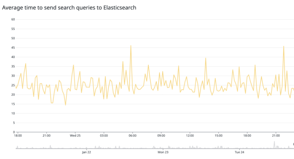
About 55% of all searches on docs.github.com are multi-term queries, for example, actions rest. Meaning that in roughly half the cases, we can use the simplified queries because we can omit things like the match_phrase parts of the total query.
Before getting into the various combinations of searches, there’s a section later about what “explicit” means. Essentially, each field is indexed twice. E.g. title and title_explicit. It’s the same content underneath but it’s tokenized differently, which affects how it matches to queries—and that difference is exploited by having different boostings.
The nodes that make up the matrix are:
Fields:
title(the<h1>text)headings(the<h2>texts)content(the bulk of the article text)
Analyzer:
- explicit (no stemming and no synonyms)
- regular (full Snowball stemming and possibly synonyms)
Matches: (on multi-term queries)
match_phrasematchwithOR(docs that contain “foo” OR “bar”)matchwithAND(docs that contain “foo” AND “bar”)
Each of these combinations has a unique boost number, which boosts the ranking of the matched result. The actual number doesn’t matter much, but what matters is that the boost numbers are different from each other. For example, a match on the title has a slightly higher boost than a match on the content. And a match where all words are present has a slightly higher boost than when only some of the words match. Another example: if the search term is docker action, the users would prefer to see “Creating a Docker container action” ahead of “Publishing Docker images” or “Metadata syntax for GitHub Actions.”
Each of the above nodes has a boost calculation that looks something like this:
const BOOST_PHRASE = 10.0
const BOOST_TITLE = 4.0
const BOOST_HEADINGS = 3.0
const BOOST_CONTENT = 1.0
const BOOST_AND = 2.5
const BOOST_EXPLICIT = 3.5

...
match_phrase: { title_explicit: { boost: BOOST_EXPLICIT * BOOST_PHRASE * BOOST_TITLE, query } },
match: { headings: { boost: BOOST_HEADINGS * BOOST_AND, query, operator: 'AND' } },
...
If you exclusively print out what the boost value becomes for each node in the matrix you get:
[
  { match_phrase: { title_explicit: 140 } },
  { match_phrase: { title: 40 } },
  { match_phrase: { headings_explicit: 105 } },
  { match_phrase: { headings: 30 } },
  { match_phrase: { content: 10 } },
  { match_phrase: { content_explicit: 35 } },
  { match: { title_explicit: 35, operator: 'AND' } },
  { match: { headings_explicit: 26.25, operator: 'AND' } },
  { match: { content_explicit: 8.75, operator: 'AND' } },
  { match: { title: 10, operator: 'AND' } },
  { match: { headings: 7.5, operator: 'AND' } },
  { match: { content: 2.5, operator: 'AND' } },
  { match: { title_explicit: 14 } },
  { match: { headings_explicit: 10.5 } },
  { match: { content_explicit: 3.5 } },
  { match: { title: 4 } },
  { match: { headings: 3 } },
  { match: { content: 1 } },
  { fuzzy: { title: 0.1 } }
]
So that’s what we send to Elasticsearch. It’s like a complex wishlist saying, “I want a bicycle for Christmas. But if you have a pink one, even better. And a pink one with blue stripes is even better still. Actually, bestest would be a pink one with blue stripes and a brass bell.”
What’s important, in terms of an ideal implementation and search result for users, is that we use our human and contextual intelligence to define these parameters. Some of it is fairly obvious and some is more subtle. For example, we think a phrase match on the title without the need for stemming is the best possible match, so that gets the highest boost.
Why explicit boost is important
If someone types “creating repositories” it should definitely match a title like “Create a private GitHub repository” because of the stems creating => creat <= create and repositories => repository <= repository. We should definitely include those matches that take stemming into account. But if there’s an article that explicitly uses the words that match what the user typed, like “Creating private GitHub repositories,” then we want to boost that article’s ranking because we think that’s more relevant to the searcher.
Another good example of this is the special keyword working-directory which is an actual exact term that can appear inside the content. If someone searches for working-directory, we don’t want to let an (example) title like “Directories that work” overpower the rankings when working-directory and “Directories that work” are both deconstructed to the same two stems [ 'work', 'directori' ].
The solution we rely on is to make two matches: one with stemming and one without. Each one has a different boost. It’s similar to saying, “I’m looking for a ‘Peter’ but if there’s a ‘Petter’ or ‘Pierre’ or ‘Piotr’ that’ll also do. But ideally, ‘Peter’ first and foremost. In fact, give me all the results, but ‘Peter’ first.” So this is what we do. The stemming is great but it can potentially “overpower” search results. This helps with specific keywords that might appear to be English prose. For example “working-directory” even looks like a regular English expression but it’s actually a hardcoded specific keyword.
In terms of code, it looks like this:
// Creating the index...
await client.indices.create({
  mappings: {
    properties: {
      url: { type: 'keyword' },
      title: { type: 'text', analyzer: 'text_analyzer', norms: false },
      title_explicit: { type: 'text', analyzer: 'text_analyzer_explicit', norms: false },
      content: { type: 'text', analyzer: 'text_analyzer' },
      content_explicit: { type: 'text', analyzer: 'text_analyzer_explicit' },
      // ...snip...
      },
    },
    // ...snip...
  })
// Searching...
matchQueries.push(
  ...[
    { match: { title_explicit: { boost: BOOST_EXPLICIT * BOOST_TITLE, query } } },
    { match: { content_explicit: { boost: BOOST_EXPLICIT * BOOST_CONTENT, query } } },
    { match: { title: { boost: BOOST_TITLE, query } } },
    { match: { content: { boost: BOOST_CONTENT, query } } },
    // ...snip...
])
Ranking is not that easy
Search is quickly becoming an art. It’s not enough to just match the terms and display a list of documents that match the terms of the input. For starters, the ranking is crucially important. This is especially true when a search term yields tens or hundreds of matching documents. Years of depending on Google has taught us all to expect the first search result to be the one we want.
To make this a great experience, we try to infer which document the user is genuinely looking for by using pageview metrics as a way to determine which page is most popular. Sure, if the most popular one is offered first, and gets the clicks, it’ll just get even more popular, but it’s a start. We get a lot of pageviews from users Googling something. But we also get regular pageview metrics from users simply navigating themselves to the pages they have figured out has the best information for them.
At the moment, we gather pageview metrics for the top 1,000 most popular URLs. Then we rank them and normalize it to a number between (and including) 0.0 to 1.0. Whatever the number is we add +1.0 and then we multiply this number in Elasticsearch with the match score.
Suppose a search query finds two documents that match, and their match score is 15.6 and 13.2 based on the search implementation mentioned above. Now, suppose that match of 13.2 is on a popular page, its popularity number might be 0.75, so it becomes 13.2 * (1 + 0.75) = 23.1. And the other one that matched a little bit better, has a popularity number of 0.44, so its final number becomes 15.6 * (1 + 0.44) = 22.5, which is less. In conclusion, it gives documents that might not be term-for-term as “matchy” as others a chance to rise above. This also ensures that a hugely popular document that only matched vaguely in the content won’t “overpower” other matches that might have matched in the title.
It’s a tricky challenge, but that’s what makes it so much fun. You have to bake in some human touch to the code as a way of trying to think like your users. It’s also an algorithm that will never reach perfection because even with more and better metrics, the landscape of users and where they come from, is constantly changing. But we’ll try to keep up.
What’s next?
Elasticsearch has a functionality where you can define aliases for words, which they call synonyms. (For example, repo = repository.) The challenge with this feature is how it’s managed and maintained by writers in a convenient and maintainable way.
Currently at GitHub, we base our popularity numbers by pageview metrics. It would be interesting to dig deeper into which page the user lands on. As an example, suppose the reader isn’t sure how to find what they need, so they start on a product landing page (we have about 20 of those) and slowly make their way deeper into the content and finally arrive on the page that supplied the knowledge or answer they want. This process would give each page an equal measure, and that’s not great.
Another exciting idea is to record all the times a search result URL is not clicked on, especially when it shows up higher in the ranking. That would decrease the risk of popular listings only getting more popular. If you record when something is “corrected” by humans, that could be a very powerful signal.
You could also tailor the underlying search based on other contextual variables. For example, if a user is currently inside the REST API docs you could infer that REST API-related docs are slightly preferred when searching for something ambiguous like “billing” (i.e. prefer REST API “About billing” not Billing and payments “Setting your billing email.”).
What are you looking for next? Have you tried the search on https://docs.github.com recently and found that it wasn’t giving you the best search result? Please let us know and get in touch.
[$] An EEVDF CPU scheduler for Linux
Post Syndicated from original https://lwn.net/Articles/925371/
The kernel’s completely fair scheduler
(CFS) has the job of managing the allocation of CPU time for most of
the processes running on most Linux systems. CFS was merged for the 2.6.23
release in 2007 and has, with numerous ongoing tweaks, handled the job
reasonably well ever since. CFS is not perfect, though, and there are some
situations it does not handle as well as it should. The EEVDF
scheduler, posted by Peter Zijlstra, offers the possibility of
improving on CFS while reducing its dependence on often-fragile heuristics.
[The Lost Bots] S03E01: Tech stack consolidation and bacon
Post Syndicated from Amy Hunt original https://blog.rapid7.com/2023/03/09/the-lost-bots-s03e01-tech-stack-consolidation-and-bacon/
![]()
It’s 2023, and according to Gartner, ESG, and everybody else, the vendor consolidation trend continues. Throwing tools at the problem isn’t working well, and creates problems of its own.
So, this season of “Lost Bots” starts with Jeffrey Gardner, Detection and Response Practice Advisor and Stephen Davis, Lead D&R Sales Technical Advisor, talking the many upsides of consolidation—deals, integration, one throat to choke—and what they call the “gotchas” too.
At the 4:00 mark, there’s a good discussion of consolidation of layers vs. function. Pay attention: some consolidation decisions can actually increase your risk. And because these guys are more than valuable fonts of free tips, the episode is packed with air quotes, bacon, and other surprises.
Rust 1.68.0 released
Post Syndicated from original https://lwn.net/Articles/925732/
Version
1.68.0 of the Rust language has been released. Changes include the
stabilization of the “sparse” Cargo protocol, the ability for (some)
applications to recover from memory-allocation failures, and “local Pin
construction”:
The new pin! macro constructs a
Pin<&mut T> from a T expression,
anonymously captured in local state. This is often called
stack-pinning, but that “stack” could also be the captured state of
an async fn or block.
Security updates for Thursday
Post Syndicated from original https://lwn.net/Articles/925723/
Security updates have been issued by CentOS (kernel, pesign, samba, and zlib), Oracle (kernel), Slackware (httpd), SUSE (emacs, libxslt, nodejs12, nodejs14, nodejs16, openssl, poppler, python-py, python-wheel, xen, and xorg-x11-server), and Ubuntu (linux-gcp-5.4, linux-gkeop, opusfile, and samba).
The SSD Edition: 2022 Drive Stats Review
Post Syndicated from original https://www.backblaze.com/blog/ssd-edition-2022-drive-stats-review/
Welcome to the 2022 SSD Edition of the Backblaze Drive Stats series. The SSD Edition focuses on the solid state drives (SSDs) we use as boot drives for the data storage servers in our cloud storage platform. This is opposed to our traditional Drive Stats reports which focus on our hard disk drives (HDDs) used to store customer data.
We started using SSDs as boot drives beginning in Q4 of 2018. Since that time, all new storage servers and any with failed HDD boot drives have had SSDs installed. Boot drives in our environment do much more than boot the storage servers. Each day they also read, write, and delete log files and temporary files produced by the storage server itself. The workload is similar across all the SSDs included in this report.
In this report, we look at the failure rates of the SSDs that we use in our storage servers for 2022, for the last 3 years, and for the lifetime of the SSDs. In addition, we take our first look at the temperature of our SSDs for 2022, and we compare SSD and HDD temperatures to see if SSDs really do run cooler.
Overview
As of December 31, 2022, there were 2,906 SSDs being used as boot drives in our storage servers. There were 13 different models in use, most of which are considered consumer grade SSDs, and we’ll touch on why we use consumer grade SSDs a little later. In this report, we’ll show the Annualized Failure Rate (AFR) for these drive models over various periods of time, making observations and providing caveats to help interpret the data presented.
The dataset on which this report is based is available for download on our Drive Stats Test Data webpage. The SSD data is combined with the HDD data in the same files. Unfortunately, the data itself does not distinguish between SSD and HDD drive types, so you have to use the model field to make that distinction. If you are just looking for SSD data, start with Q4 2018 and go forward.
2022 Annual SSD Failure Rates
As noted, at the end of 2022, there were 2,906 SSDs in operation in our storage servers. The table below shows data for 2022. Later on we’ll compare the 2022 data to previous years.

Observations and Caveats
- For 2022, seven of the 13 drive models had no failures. Six of the seven models had a limited number of drive days—less than 10,000—meaning that there is not enough data to make a reliable projection about the failure rates of those drive models.
- The Dell SSD (model: DELLBOSS VD) has zero failures for 2022 and has over 100,000 drive days for the year. The resulting AFR is excellent, but this is an M.2 SSD mounted on a PCIe card (half-length and half-height form factor) meant for server deployments, and as such it may not be generally available. By the way, BOSS stands for Boot Optimized Storage Solution.
- Besides the Dell SSD, three other drive models have over 100,000 drive days for the year, so there is sufficient data to consider their failure rates. Of the three, the Seagate (model: ZA250CM10003, aka: Seagate BarraCuda 120 SSD ZA250CM10003) has the lowest AFR at 0.73%, with the Crucial (model: CT250MX500SSD1) coming in next with an AFR of 1.04% and finally, the Seagate (model: ZA250CM10002, aka: Seagate BarraCuda SSD ZA250CM10002) delivers an AFR of 1.98% for 2022.
Annual SSD Failure Rates for 2020, 2021, and 2022
The 2022 annual chart above presents data for events that occurred in just 2022. Below we compare the 2022 annual data to the 2020 and 2021 (respectively) annual data where the data for each year represents just the events which occurred during that period.
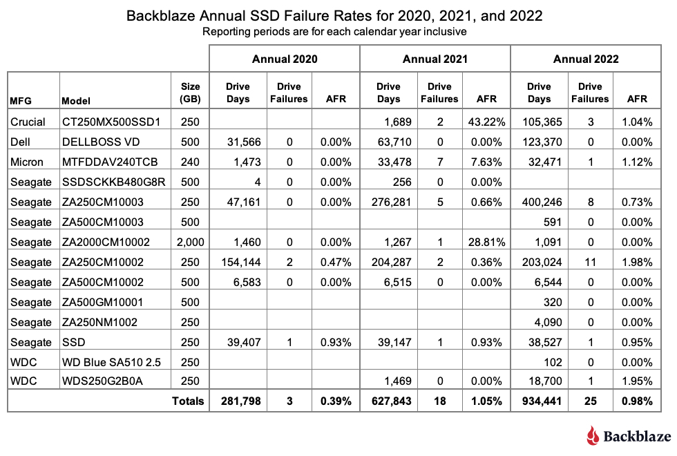
Observations and Caveats
- As expected, the Crucial drives (model: CT250MX500SSD1) recovered nicely in 2022 after having a couple of early failures in 2021. We expect that trend to continue.
- Four new models were introduced in 2022, although none have a sufficient number of drive days to discern any patterns even though none of the four models have experienced a failure as of the end of 2022.
- Two of the 250GB Seagate drives have been around all three years, but they are going in different directions. The Seagate drive (model: ZA250CM10003) has delivered a sub-1% AFR over all three years. While the AFR for the Seagate drive (model: ZA250CM10002) slipped in 2022 to nearly 2%. Model ZA250CM10003 is the newer model of the two by about a year. There is little difference otherwise except the ZA250CM10003 uses less idle power, 116mW versus 185mW for the ZA250CM10002. It will be interesting to see how the younger model fares over the next year. Will it follow the trend of its older sibling and start failing more often, or will it chart its own course?
SSD Temperature and AFR: A First Look
Before we jump into the lifetime SSD failure rates, let’s talk about SSD SMART stats. Here at Backblaze, we’ve been wrestling with SSD SMART stats for several months now, and one thing we have found is there is not much consistency on the attributes, or even the naming, SSD manufacturers use to record their various SMART data. For example, terms like wear leveling, endurance, lifetime used, life used, LBAs written, LBAs read, and so on are used inconsistently between manufacturers, often using different SMART attributes, and sometimes they are not recorded at all.
One SMART attribute that does appear to be consistent (almost) is drive temperature. SMART 194 (raw value) records the internal temperature of the SSD in degrees Celsius. We say almost, because the Dell SSD (model: DELLBOSS VD) does not report raw or normalized values for SMART 194. The chart below shows the monthly average temperature for the remaining SSDs in service during 2022.
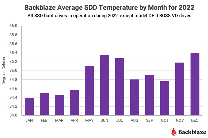
Observations and Caveats
- There were an average of 67,724 observations per month, ranging from 57,015 in February to 77,174 in December. For 2022, the average temperature varied only one degree Celsius from the low of 34.4 degrees Celsius to the high of 35.4 degrees Celsius over the period.
- For 2022, the average temperature was 34.9 degrees Celsius. The average temperature of the hard drives in the same storage servers over the same period was 29.1 degrees Celsius. This difference seems to fly in the face of conventional wisdom that says SSDs run cooler than HDDs. One possible reason is that, in all of our storage servers, the boot drives are further away from the cool aisle than the data drives. That is, the data drives get the cool air first. If you have any thoughts, let us know in the comments.
- The temperature variation across all drives for 2022 ranged from 20 degrees Celsius (four observations) to 61 degrees Celsius (one observation). The chart below shows the observations for the SSD’s across that temperature range.

The shape of the curve should look familiar: it’s a bell curve. We’ve seen the same type of curve when plotting the temperature observations of the storage server hard drives. The SSD curve is for all operational SSD drives, except the Dell SSDs. We attempted to plot the same curve for the failed SSDs, but with only 25 failures in 2022, the curve was nonsense.
Lifetime SSD Failure Rates
The lifetime failure rates are based on data from the entire time the given drive model has been in service in our system. This data goes back as far as Q4 2018, although most of the drives were put in service in the last three years. The table below shows the lifetime AFR for all of the SSD drive models in service as of the end of 2022.

Observations and Caveats
- The overall Lifetime AFR was 0.89% as of the end of 2022. This is lower than the Lifetime AFR 1.04% as of the end of 2021.
- There are several very large confidence intervals. That is due to the limited amount of data (drive days) for those drive models. For example, there are only 104 drive days for the WDC model WD Blue SA510 2.5. As we accumulate more data, those confidence intervals should become more accurate.
- We like to see a confidence interval of 1.0% or less for a given drive model. Only three drive models met this criteria:
- Dell model DELLBOSS VD: lifetime AFR–0.00%
- Seagate model ZA250CM10003: lifetime AFR–0.66%
- Seagate model ZA250CM10002: lifetime AFR–0.96%
- The Dell SSD, as noted earlier in this report, is an M.2 SSD mounted on a PCIe card and may not be generally available. The two Seagate drives are consumer level SSDs. In our case, a less expensive consumer level SSD works for our needs as there is no customer data on a boot drive, just boot files as well as log and temporary files. More recently as we have purchased storage servers from Supermicro and Dell, they bundle all of the components together into a unit price per storage server. If that bundle includes enterprise class SSDs or an M.2 SSD on a PCIe card, that’s fine with us.
The SSD Stats Data
We acknowledge that 2,906 SSDs is a relatively small number of drives on which to perform our analysis, and while this number does lead to wider than desired confidence intervals, it’s a start. Of course we will continue to add SSD boot drives to the study group, which will improve the fidelity of the data presented. In the meantime, we expect our readers will apply their usual skeptical lens to the data presented and use it accordingly.
The complete dataset used to create the information used in this review is available on our Hard Drive Test Data page. As noted earlier you’ll find SSD and HDD data in the same files, and you’ll have to use the model number to distinguish one record from another. You can download and use this data for free for your own purpose. All we ask are three things: 1) you cite Backblaze as the source if you use the data, 2) you accept that you are solely responsible for how you use the data, and 3) you do not sell this data to anyone; it is free.
Good luck, and let us know if you find anything interesting.
The post The SSD Edition: 2022 Drive Stats Review appeared first on Backblaze Blog | Cloud Storage & Cloud Backup.
Building serverless Java applications with the AWS SAM CLI
Post Syndicated from James Beswick original https://aws.amazon.com/blogs/compute/building-serverless-java-applications-with-the-aws-sam-cli/
This post was written by Mehmet Nuri Deveci, Sr. Software Development Engineer, Steven Cook, Sr.Solutions Architect, and Maximilian Schellhorn, Solutions Architect.
When using Java in the serverless environment, the AWS Serverless Application Model Command Line Interface (AWS SAM CLI) offers an easier way to build and deploy AWS Lambda functions. You can either use the default AWS SAM build mechanism or tailor the build behavior to your application needs.
Since Java offers a variety of plugins and tools for building your application, builders usually have custom requirements for their build setup. In addition, when targeting GraalVM or non-LTS versions of the JVM, the build behavior requires additional configuration to build a Lambda custom runtime.
This blog post provides an overview of the common ways to build Java applications for Lambda with the AWS SAM CLI. This allows you to make well-informed decisions based on your projects’ requirements. This post focuses on Apache Maven, however the same concepts apply for Gradle.
You can find the source code for these examples in the GitHub repo.
Overview
The following diagram provides an overview of the build and deployment process with AWS SAM CLI. The default behavior includes the following steps:
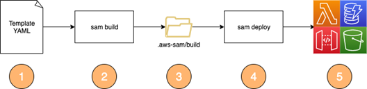
- Define your infrastructure resources such as Lambda functions, Amazon DynamoDB Tables, Amazon S3 buckets, or an Amazon API Gateway endpoint in a template.yaml file.
- The CLI command “sam build” builds the application based on the chosen runtime and configuration within the template.
- The sam build command populates the .aws-sam/build folder with the built artifacts (for example, class files or jars).
- The sam deploy command uploads your template and function code from the .aws-sam/build folder and starts an AWS CloudFormation deployment.
- After a successful deployment, you can find the provisioned resources in your AWS account.
Using the default Java build mechanism in AWS SAM CLI
AWS SAM CLI supports building Serverless Java functions with Maven or Gradle. You must use one of the supported Java runtimes (java8, java8.al2, java11) and your function’s resource CodeUri property must point to a source folder.

AWS SAM CLI ships with default build mechanisms provided by the aws-lambda-builders project. It is therefore not required to package or build your application in advance and any customized build steps in pom.xml will not be used. For example, by default the AWS SAM Maven Lambda Builder triggers the following steps:
- mvn clean install to build the function.
- mvn dependency:copy-dependencies -DincludeScope=runtime -Dmdep.prependGroupId=true to prepare dependency jar files.
- Class files in target/classes and dependency jar archives in target/dependency are copied to the final build artifact location in .aws-sam/build/{ResourceLogicalId}.
Start the build process by running the following command from the directory where the template.yaml resides:
sam buildThis results in the following outputs:

The .aws-sam build folder contains the necessary classes and libraries to run your application. The transformed template.yaml file points to the build artifacts directory (instead of pointing to the original source directory).
Run the following command to deploy the resources to AWS:
sam deploy --guidedThis zips the HelloWorldFunction directory in .aws-sam/build and uploads it to the Lambda service.
Building Uber-Jars with AWS SAM CLI
A popular way for building and packaging Java projects, especially when using frameworks such as Micronaut, Quarkus and Spring Boot is to create an Uber-jar or Fat-jar. This is a jar file that contains the application class files with all the dependency class files within a single jar file. This simplifies the deployment and management of the application artifact.
Frameworks typically provide a Maven or Gradle setup that produces an Uber-jar by default. For example, by using the Apache Maven Shade plugin for Maven, you can configure Uber-jar packaging:
<build>
  <plugins>
    <plugin>
      <groupId>org.apache.maven.plugins</groupId>
      <artifactId>maven-shade-plugin</artifactId>
      <version>3.4.1</version>
      <executions>
 	 <execution>
 	   <phase>package</phase>
 	     <goals>
 	       <goal>shade</goal>
 	     </goals>
 	 </execution>
      </executions>
     </plugin>
  </plugins>
</build>
The maven-shade-plugin modifies the package phase of the Maven build to produce the Uber-jar file in the target directory.
To build and package an Uber-jar with AWS SAM, you must customize the AWS SAM CLI build process. You can do this by using a Makefile to replace the default steps discussed earlier. Within the template.yaml, declare a Metadata resource attribute with a BuildMethod entry. The sam build process then looks for a Makefile within the CodeUri directory.

The Makefile is responsible for building the artifacts required by AWS SAM to deploy the Lambda function. AWS SAM runs the target in the Makefile. This is an example Makefile:
build-HelloWorldFunctionUberJar:
 	mvn clean package
 	mkdir -p $(ARTIFACTS_DIR)/lib
 	cp ./target/HelloWorld*.jar $(ARTIFACTS_DIR)/lib/
The Makefile runs the Maven clean and package goals that build Uber-jar in the target directory via the Apache Maven Plugin. As the Lambda Java runtime loads jar files from the lib directory, you can copy the uber-jar file to the $ARTIFACTS_DIR/lib directory as part of the build steps.
To build the application, run:
sam buildThis triggers the customized build step and creates the following output resources:

The deployment step is identical to the previous example.
Running the build process inside a container
AWS SAM provides a mechanism to run the application build process inside a Docker container. This provides the benefit of not requiring your build dependencies (such as Maven and Java) to be installed locally or in your CI/CD environment.
To run the build process inside a container, use the command line options –use-container and optionally –build-image. The following diagram outlines the modified build process with this option:

- Similar to the previous examples, the directory with the application sources or the Makefile is referenced.
- To run the build process inside a Docker container, provide the command line option:
sam build –-use-container - By default, AWS SAM uses images for container builds that are maintained in the GitHub repo aws/aws-sam-build-images. AWS SAM pulls the container image depending on the defined runtime. For this example, it pulls the public.ecr.aws/sam/build-java11 image, which has prerequisites such as Maven and Java11 pre-installed to build the application. In addition, the source code folder is mounted in the container and the Makefile target or default build mechanism is run within the container.
- The final artifacts are delivered to the.aws-sam/build directory on the local file system. If you are using a Makefile, you can copy the final artifact to the $ARTIFACTS_DIR.
- The sam deploy command uploads the template and function code from the .aws-sam/build directory and starts a CloudFormation deployment.
- After a successful deployment, you can find the provisioned resources in your AWS account.
To test the behavior, run the previous examples with the –use-container option. No additional changes are needed.
Using your own base build images for creating custom runtimes
When you are targeting a non-supported Lambda runtime, such as a non-LTS Java version or natively compiled GraalVM native images, you can create your own build image with the necessary dependencies installed.
For example, to build a native image with GraalVM, you must have GraalVM and the native image tool installed when building your application.
To create a custom image:
- Create a Dockerfile with the needed dependencies:
#Use the official AWS SAM base image or Amazon Linux 2 as a starting point FROM public.ecr.aws/sam/build-java11:latest-x86_64 #Install GraalVM dependencies ENV GRAAL_VERSION 22.2.0 ENV GRAAL_FOLDERNAME graalvm-ce-java11-${GRAAL_VERSION} ENV GRAAL_FILENAME graalvm-ce-java11-linux-amd64-${GRAAL_VERSION}.tar.gz RUN curl -4 -L https://github.com/graalvm/graalvm-ce-builds/releases/download/vm-22.2.0/graalvm-ce-java11-linux-amd64-22.2.0.tar.gz | tar -xvz RUN mv $GRAAL_FOLDERNAME /usr/lib/graalvm RUN rm -rf $GRAAL_FOLDERNAME #Install Native Image dependencies RUN /usr/lib/graalvm/bin/gu install native-image RUN ln -s /usr/lib/graalvm/bin/native-image /usr/bin/native-image RUN ln -s /usr/lib/maven/bin/mvn /usr/bin/mvn #Set GraalVM as default ENV JAVA_HOME /usr/lib/graalvm - Build your image locally or upload it to a container registry:
docker build . -t sam/custom-graal-image - Use AWS SAM build with the build image argument to provide your custom image:
sam build --use-container --build-image sam/custom-graal-image
You can find the source code and an example Dockerfile, Makefile, and pom.xml for GraalVM native images in the GitHub repo.
When you use the official AWS SAM build images as a base image, you have all the necessary tooling such as Maven, Java11 and the Lambda builders installed. If you want to use a more customized approach and use a different base image, you must install these dependencies.
For an example, check the GraalVM with Java 17 cookiecutter template. In addition, there are multiple additional components involved when building custom runtimes, which are outlined in “Build a custom Java runtime for AWS Lambda”.
To avoid providing the command line options on every build, include them in the samconfig.toml file:
[default.build.parameters]
use_container = true
build_image = ["public.ecr.aws/sam/build-java11:latest-x86_64"]
For additional information, refer to the official AWS SAM CLI documentation.
Deploying the application without building with AWS SAM
There might be scenarios where you do not want to rely on the build process offered by AWS SAM. For example, when you have highly customized or established build processes, or advanced dependency caching or visibility requirements.
In this case, you can still use the AWS SAM CLI commands such as sam local and sam deploy. But you must point your CodeUri property directly to the pre-built artifact (instead of the source code directory):
HelloWorldFunctionSkipBuild:
  Type: AWS::Serverless::Function
  Properties:
    CodeUri: HelloWorldFunction/target/HelloWorld-1.0.jar
    Handler: helloworld.App::handleRequest
In this case, there is no need to use the sam build command, since the build logic is outside of AWS SAM CLI:

Here, the sam build command fails because it looks for a source folder to build the application. However, there might be cases where you have a mixed setup that includes some functions that point to pre-built artifacts and others that are built by AWS SAM CLI. In this scenario, you can mark those functions to explicitly skip the build process by adding the following SkipBuild flag in the Metadata section of your resource definition:
HelloWorldFunctionSkipBuild:
  Type: AWS::Serverless::Function
  Properties:
    CodeUri: HelloWorldFunction/target/HelloWorld-1.0.jar
    Handler: helloworld.App::handleRequest
    Runtime: java11
  Metadata:
    SkipBuild: True
Conclusion
This blog post shows how to build Java applications with the AWS SAM CLI. You learnt about the default build mechanisms, and how to customize the build behavior and abstract the build process inside a container environment. Visit the GitHub repository for the example code templates referenced in the examples.
To learn more, dive deep into the AWS SAM documentation. For more serverless learning resources, visit Serverless Land.
Server-side rendering micro-frontends – UI composer and service discovery
Post Syndicated from James Beswick original https://aws.amazon.com/blogs/compute/server-side-rendering-micro-frontends-ui-composer-and-service-discovery/
This post is written by Luca Mezzalira, Principal Specialist Solutions Architect, Serverless.
The previous blog post describes the architecture for creating a server-side rendering micro-frontend in AWS. This and subsequent posts explain the different parts that compose this architecture in detail. The code for the example is available on a AWS Samples GitHub repository.
For context, this post covers the infrastructure related to the UI composer, and why you need an Amazon S3 bucket for storing static assets:
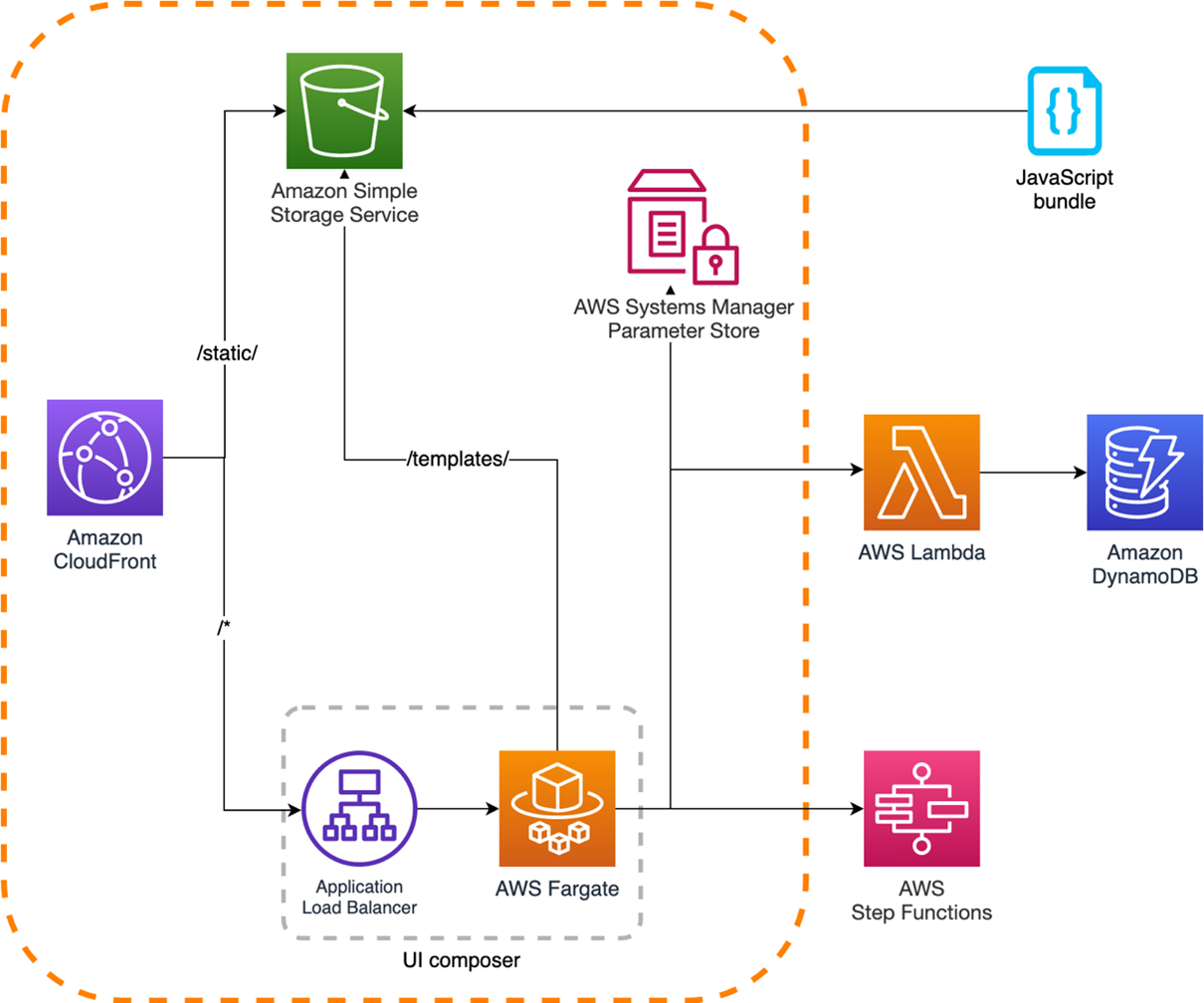
The rest of the series explores the micro-frontends composition, how to design micro-frontends using serverless services, different caching and performance optimization strategies, and the organization structure implications associated with frontend distributed systems.
A user’s request journey
The best way to navigate through this distributed system is by simulating a user request that touches all the parts implemented in the architecture.
The application example shows a product details page of a hypothetical ecommerce platform:

When a user selects an article from the catalog page, the DNS resolves the URL to an Amazon CloudFront distribution that is the reference CDN for this project.
The request is immediately fulfilled if the page is cached. Therefore, no additional logic is requested by the cloud infrastructure and the response is fast (less than the 500 ms shown in this example).
When the page is not available in the CloudFront points of presence (PoPs), the request is forwarded to the Application Load Balancer (ALB). It arrives at the AWS Fargate cluster where the UI Composer generates the page for fulfilling the request.
Using CloudFront in the architecture
CDNs are known for accelerating application delivery thanks to caching static files from nearby PoPs. CloudFront can also accelerate uncacheable content such as dynamic APIs or personalized content.
With a network of over 450 points of presence, CloudFront terminates user TCP/TLS connections within 20-30 milliseconds on average. Traffic to origin servers is carried over the AWS global network instead of the public internet. This infrastructure is a purpose-built, highly available, and low-latency private infrastructure built on a global, fully redundant, metro fiber network that is linked via terrestrial and trans-oceanic cables across the world. In addition to terminating connections close to users, CloudFront accelerates dynamic content thanks to modern internet protocols such as QUIC and TLS1.3, and persisting TCP connections to the origin servers.
CloudFront also has security benefits, offering protection in AWS against infrastructure DDoS attacks. It integrates with AWS Web Application Firewall and AWS Shield Advanced, giving you controls to block application-level DDoS attacks. CloudFront also offers native security controls such as HTTP to HTTPS redirections, CORS management, geo-blocking, tokenization, and managing security response headers.
UI Composer application logic
When the request is not fulfilled by the CloudFront cache, it is routed to the Fargate cluster. Here, multiple tasks compute and serve the page requested.
This example uses Fastify, a fast Node.js framework that is gaining popularity among the Node.js community. When the web server initializes, it loads external parameters and the template for composing a page.
const start = async () => {
  try {
    //load parameters
    MFElist = await init();
    //load catalog template
    catalogTemplate = await loadFromS3(MFElist.template, MFElist.templatesBucket)
    await fastify.listen({ port: PORT, host: '0.0.0.0' })
  } catch (err) {
    fastify.log.error(err)
    process.exit(1)
  }
}
To maintain team independence and avoid redeploying the UI composer for every application change, the HTML templates are loaded from an S3 bucket. All teams responsible for micro-frontends in the same page can position their micro-frontends into the right place of the HTML template and delegate the composition task to the UI composer.
In this demo, the initial parameters and the catalog template are retrieved once. However, in a real scenario, it’s more likely you retrieve the parameters at initialization and at a regular cadence. The template might be loaded at runtime for every request or have another background routine fetching the initialization parameters in a similar way.
When the request reaches the product details route, the web application logic calls a transformTemplate function. It passes the catalog template, retrieved from the S3 bucket at the server initialization. It returns a 200 response if the page is composed without any issues.
fastify.get('/productdetails', async(request, reply) => {
  try{
    const catalogDetailspage = await transformTemplate(catalogTemplate)
    responseStream(catalogDetailspage, 200, reply)
  } catch(err){
    console.log(err)
    throw new Error(err)
  }
})
The page composition is the key responsibility of the UI composer. There are several viable approaches for composing micro-frontends in a server-side rendering system, covered in the next post.
Micro-frontends discovery
To decouple workloads for multiple teams, you must use architectural patterns that support it. In a microservices architecture, a pattern that allows independent evolution of a service without coupling the DNS or IP to any microservice is the service discovery pattern.
In this example, AWS System Managers Parameters Store acts as a services registry. Every micro-frontend available in the workload registers itself once the infrastructure is provisioned.
In this way, the UI composer can request the micro-frontend ID found inside the HTML template. It can retrieve the correct way to consume the micro-frontend API using an ARN or a remote HTTP URL, for instance.

Using ARN over HTTP requests inside the workload network can help you to reduce the latency thanks to fewer network hops. Moreover, the security is delegated to IAM policies providing a robust security implementation.
The UI composer takes care to retrieve the micro-frontends endpoints at runtime before loading them into the HTML template. This is a simpler yet powerful approach for maintaining the boundaries within your organization and allowing independent teams to evolve their architecture autonomously.
Micro-frontends discovery evolution
Using Parameter Store as a service discovery system, you can deploy a new micro-frontend by adding a new key-value into the service discovery.
A more sophisticated option could be creating a service that acts as a registry and also shapes the traffic towards different micro-frontends versions using deployment strategies like canary releases or blue/green deployments.
You can start iteratively with a simple key-value store system and evolve the architecture with a more complex approach when the workload requires, providing a robust way to roll out micro-frontends services in your system.
When this is in place, it’s likely to increase the release cadence of your micro-frontends. This is because developers often feel safer releasing in production without affecting the entire user base and they can run tests alongside real traffic.
Performance considerations
This architecture uses Fargate for composing the micro-frontends instead of Lambda functions. This allows incremental rendering offered by browsers, displaying the HTML page partially before it’s completely returned.
Consider a scenario where a micro-frontend takes longer to render due to a downstream dependency or a faulty version deployed into production. Without the streaming capability, you must wait until all the micro-frontends responses arrive, buffer them in memory, compose the page and then send the final output to the browser.
Instead, by using the streaming API offered by Node.js frameworks, you can send a partial HTML page (for example, the head tag and subsequently the rest of the page), to be rendered by a browser.
Streaming also improves server overhead, because the servers don’t have to buffer entire pages. By incrementally flushing data to browsers, servers keep memory pressure low, which lets them process more requests and save overhead costs.
However, in case your workload doesn’t require these capabilities, one or multiple Lambda functions might be suitable for your project as well, reducing the infrastructure management complexity to handle.
Conclusion
This post looks at how to use the UI Composer and micro-frontends discoverability. Once this part is developed, it won’t need to change regularly. This represents the foundation for building server-side rendering micro-frontends using HTML-over-the-wire. There might be other approaches to follow for other frameworks such as Next.js due to the architectural implementation of the framework itself.
The next post will cover how the UI composer includes micro-frontends output inside an HTML template.
For more serverless learning resources, visit Serverless Land.