It’s always been the case that specific industries are subject to their own security standards when it comes to protecting sensitive data. You’ve probably heard of the complex rules and regulations around personal health information and credit card data, for example. Law enforcement agencies do some of the most specialized work possible, so the entire world of criminal justice is subject to its own policies and procedures. Here’s what you need to know about Criminal Justice Information Services and the CJIS Security Policy.
The History of Criminal Justice Information Services
Criminal Justice Information Services (CJIS) is the largest division of the FBI. It was originally established in 1992 to give law enforcement agencies, national security teams, and the intelligence community shared access to a huge repository of highly sensitive data like fingerprints and active case reports. The CJIS Security Policy exists to safeguard that information by defining protocols for the entire data life cycle wherever it exists, both at rest and in transit. It’s easy to see how important it is for law enforcement agencies to need quick and secure access to this case critical data, but it’s also clear just how detrimental that data could be if it got into the wrong hands.
What Is Criminal Justice Information?
To get a better sense of the CJIS Security Policy and how it works, let’s start by looking at the data it covers. These are the five types of data that qualify as criminal justice information (CJI):
Biometric data: Data points that can be used to identify a unique individual, like fingerprints, palm prints, iris scans, and facial recognition data.
Identity history data: A text record of an individual’s civil or criminal history that can be tied to the biometric data that identifies them.
Biographic data: Information about individuals associated with a particular case, even without unique identifiers or biometric data attached.
Property data: Information about vehicles or physical property associated with a particular case and accompanied by personally identifiable information.
Case/Incident history: Data about the history of criminal incidents.
How Does CJIS Compliance Work?
The sensitivity of the types of data that qualify as CJI explains just how complicated the CJIS Security Policy is. To complicate matters further, CJIS (under the FBI and in turn the U.S. Department of Justice) issues regular updates to the Security Policy. The complexity inherent in the national policy, in combination with the pressure of keeping pace with constant changes, has meant that many law enforcement, national security, and intelligence agencies opt not to share data between agencies in lieu of taking the necessary steps to keep it safe in compliance with CJIS.
Each individual government agency is responsible for managing their own CJIS compliance. And the Security Policy applies to anyone interacting with that data, regardless of what system they use to do so or how they are associated with the agency that owns it. That means law enforcement representatives, lawyers, contractors, and private entities, for example, are all subject to the rules laid out in the CJIS Security Policy. What’s more, state governments and their respective CJIS Security Officers are responsible for managing the application of the Security Policy at the state level.
How To Achieve CJIS Compliance
Despite all this complexity, CJIS doesn’t issue any official compliance certifications. Instead, compliance with the Security Policy falls under the purview of each individual organization, agency, or government body. Having the right technical controls in place to satisfy all standardized areas of the policy—and managing those controls on an ongoing basis—is the best (and the only) way to achieve CJIS compliance. These are the 13 key areas listed in the Security Policy:
Area 1: Information Exchange Agreements
Before an agency or organization shares CJI with any other entity, both parties must establish and mutually sign a formal information exchange agreement to certify that everyone involved is in CJIS compliant.
Area 2: Awareness & Training
Any individuals interacting with CJI have to participate in annual specialized training about how they are expected to comply with the Security Policy.
Area 3: Incident Response
Every agency interacting with CJI must have an Incident Response Plan (IRP) in place to ensure their ability to identify security incidents when they occur. IRPs also outline plans to contain and remediate damage as quickly and efficiently as possible.
Area 4: Auditing & Accountability
Organizations have to monitor who accesses CJI, when they access it, and what they do with it. Establishing visibility into interactions like file access, login attempts, password changes, etc. helps dissuade bad actors from accessing data they shouldn’t and also gives agencies the forensic information they need to investigate incidents if breaches do occur.
Area 5: Access Control
Another way to ensure that only authorized users interact with CJI is to limit access based on specific attributes like job title, location, and IP address. Implementing role-based access controls helps limit the availability of CJI, so only the people who need to use that data can access it (and only when absolutely necessary).
Area 6: Identification & Authentication
Because of the rules around auditing & accountability and access control, the Security Policy also stipulates the importance of authenticating every user’s identity. CJIS’ identification & authentication rules include the use of multifactor authentication, regular password resets, and revoked credentials after five unsuccessful login attempts.
Area 7: Configuration Management
Only authorized users should be allowed to change the configuration of the systems that store CJI. This includes simple tasks like performing software updates, but it also extends to the hardware realm, for example when it comes to adding or removing devices from a network.
Area 8: Media Protection
Compliant agencies must establish policies to protect all forms of media, including putting procedures in place for the secure disposal of that media once it is no longer in use.
Area 9: Physical Protection
Any physical spaces (like on-premises server rooms, for example) should be locked, monitored by camera equipment, and equipped with alarms to prevent unauthorized access.
Area 10: System & Communications Protection
Cybersecurity best practices should be in place, including perimeter protection measures like Intrusion Prevention Systems, firewalls, and anti-virus solutions. In the category of encryption, FIPS 140-2 certification and a minimum of 128 bit strength are required.
Area 11: Formal Audits
Although the CJIS doesn’t issue compliance certifications, agencies still have to be available for formal audits by CJIS representatives (like the CJIS Audit Unit and the CJIS Systems Agency) at least once every three years.
Area 12: Personnel Security
Any personnel with access to CJI have to undergo a screening process and background checks (including fingerprinting) to ensure their fitness to handle sensitive data.
Area 13: Mobile Devices
In order to remain in compliance, organizations have to develop acceptable use policies that govern how mobile devices are used, how they connect to the internet, what applications they can have on them, and even what websites they can access. In this case, mobile devices include smartphones, tablets, and laptops that can access CJI. When representatives use mobile devices to access CJI, those devices (and that access) are subject to all the areas of the Security Policy.
How Backblaze Supports CJIS Compliance
For any organization to achieve CJIS compliance, any partner or vendor that accesses, interacts with, or stores their CJI also needs to comply with the same Security Policy standards. You guessed it: that means cloud storage providers too. It’s your job to ensure that your organization is CJIS-compliant before transmitting your data to any cloud storage provider. At Backblaze, we follow the same security standards outlined in the CJIS Security Policy so that you can trust that your CJI is protected and your agency is in compliance even while it’s being stored in Backblaze B2 Cloud Storage or via our Business Backup product.
If you own a domain that you use for email, you want to maintain the reputation and goodwill of your domain’s brand. Several industry-standard mechanisms can help prevent your domain from being used as part of a phishing attack. In this post, we’ll show you how to deploy three of these mechanisms, which visually authenticate emails sent from your domain to users and verify that emails are encrypted in transit. It can take as little as 15 minutes to deploy these mechanisms on Amazon Web Services (AWS), and the result can help to provide immediate and long-term improvements to your organization’s email security.
Phishing through email remains one of the most common ways that bad actors try to compromise computer systems. Incidents of phishing and related crimes far outnumber the incidents of other categories of internet crime, according to the most recent FBI Internet Crime Report. Phishing has consistently led to large annual financial losses in the US and globally.
Brand Indicators for Message Identification (BIMI) – This standard allows you to associate a logo with your email domain, which some email clients will display to users in their inbox. Visit the BIMI Group’s Where is my BIMI Logo Displayed? webpage to see how logos are displayed in the user interfaces of BIMI-supporting mailbox providers; Figure 1 shows a mock-up of a typical layout that contains a logo.
Mail Transfer Agent Strict Transport Security (MTA-STS) – This standard helps ensure that email servers always use TLS encryption and certificate-based authentication when they send messages to your domain, to protect the confidentiality and integrity of email in transit.
SMTP TLS reporting – This reporting allows you to receive reports and monitor your domain’s TLS security posture, identify problems, and learn about attacks that might be occurring.
Figure 1: A mock-up of how BIMI enables branded logos to be displayed in email user interfaces
These three standards require your Domain Name System (DNS) to publish specific records, for example by using Amazon Route 53, that point to web pages that have additional information. You can host this information without having to maintain a web server by storing it in Amazon Simple Storage Service (Amazon S3) and delivering it through Amazon CloudFront, secured with a certificate provisioned from AWS Certificate Manager (ACM).
Note: This AWS solution works for DKIM, BIMI, and DMARC, regardless of what you use to serve the actual email for your domains, which services you use to send email, and where you host DNS. For purposes of clarity, this post assumes that you are using Route 53 for DNS. If you use a different DNS hosting provider, you will manually configure DNS records in your existing hosting provider.
Solution architecture
The architecture for this solution is depicted in Figure 2.
Figure 2: The architecture diagram showing how the solution components interact
As described in more detail in the BIMI section of this blog post, the Verified Mark Certificate is obtained from a BIMI-qualified certificate authority and stored in the S3 bucket.
When an external email system receives a message claiming to be from your domain, it looks up BIMI records for your domain in DNS. As depicted in the diagram, a DNS request is sent to Route 53.
To retrieve the BIMI logo image and Verified Mark Certificate, the external email system will make HTTPS requests to a URL published in the BIMI DNS record. In this solution, the URL points to the CloudFront distribution, which has a TLS certificate provisioned with ACM.
A few important warnings
Email is a complex system of interoperating technologies. It is also brittle: a typo or a missing DNS record can make the difference between whether an email is delivered or not. Pay close attention to your email server and the users of your email systems when implementing the solution in this blog post. The main indicator that something is wrong is the absence of email. Instead of seeing an error in your email server’s log, users will tell you that they’re expecting to receive an email from somewhere and it’s not arriving. Or they will tell you that they sent an email, and their recipient can’t find it.
The DNS uses a lot of caching and time-out values to improve its efficiency. That makes DNS records slow and a little unpredictable as they propagate across the internet. So keep in mind that as you monitor your systems, it can be hours or even more than a day before the DNS record changes have an effect that you can detect.
This solution uses AWS Cloud Development Kit (CDK) custom resources, which are supported by AWS Lambda functions that will be created as part of the deployment. These functions are configured to use CDK-selected runtimes, which will eventually pass out of support and require you to update them.
Prerequisites
You will need permission in an AWS account to create and configure the following resources:
An Amazon S3 bucket to store the files and access logs
A CloudFront distribution to publicly deliver the files from the S3 bucket
A TLS certificate in ACM
An origin access identity in IAM that CloudFront will use to access files in Amazon S3
Lambda functions, IAM roles, and IAM policies created by CDK custom resources
You might also want to enable these optional services:
Amazon Route 53 for setting the necessary DNS records. If your domain is hosted by another DNS provider, you will set these DNS records manually.
Amazon SES or an Amazon WorkMail organization with a single mailbox. You can configure either service with a subdomain (for example, [email protected]) such that the existing domain is not disrupted, or you can create new email addresses by using your existing email mailbox provider.
BIMI has some additional requirements:
BIMI requires an email domain to have implemented a strong DMARC policy so that recipients can be confident in the authenticity of the branded logos. Your email domain must have a DMARC policy of p=quarantine or p=reject. Additionally, the domain’s policy cannot have sp=none or pct<100.
Note: Do not adjust the DMARC policy of your domain without careful testing, because this can disrupt mail delivery.
You must have your brand’s logo in Scaled Vector Graphics (SVG) format that conforms to the BIMI standard. For more information, see Creating BIMI SVG Logo Files on the BIMI Group website.
Purchase a Verified Mark Certificate (VMC) issued by a third-party certificate authority. This certificate attests that the logo, organization, and domain are associated with each other, based on a legal trademark registration. Many email hosting providers require this additional certificate before they will show your branded logo to their users. Others do not currently support BIMI, and others might have alternative mechanisms to determine whether to show your logo. For more information about purchasing a Verified Mark Certificate, see the BIMI Group website.
Note: If you are not ready to purchase a VMC, you can deploy this solution and validate that BIMI is correctly configured for your domain, but your branded logo will not display to recipients at major email providers.
What gets deployed in this solution?
This solution deploys the DNS records and supporting files that are required to implement BIMI, MTA-STS, and SMTP TLS reporting for an email domain. We’ll look at the deployment in more detail in the following sections.
Brand Indicators for Message Identification (BIMI) permits Domain Owners to coordinate with Mail User Agents (MUAs) to display brand-specific Indicators next to properly authenticated messages. There are two aspects of BIMI coordination: a scalable mechanism for Domain Owners to publish their desired Indicators, and a mechanism for Mail Transfer Agents (MTAs) to verify the authenticity of the Indicator. This document specifies how Domain Owners communicate their desired Indicators through the BIMI Assertion Record in DNS and how that record is to be interpreted by MTAs and MUAs. MUAs and mail-receiving organizations are free to define their own policies for making use of BIMI data and for Indicator display as they see fit.
If your organization has a trademark-protected logo, you can set up BIMI to have that logo displayed to recipients in their email inboxes. This can have a positive impact on your brand and indicates to end users that your email is more trustworthy. The BIMI Group shows examples of how brand logos are displayed in user inboxes, as well as a list of known email service providers that support the display of BIMI logos.
As a domain owner, you can implement BIMI by publishing the relevant DNS records and hosting the relevant files. To have your logo displayed by most email hosting providers, you will need to purchase a Verified Mark Certificate from a BIMI-qualified certificate authority.
This solution will deploy a valid BIMI record in Route 53 (or tell you what to publish in the DNS if you’re not using Route 53) and will store your provided SVG logo and Verified Mark Certificate files in Amazon S3, to be delivered through CloudFront with a valid TLS certificate from ACM.
To support BIMI, the solution makes the following changes to your resources:
A DNS record of type TXT is published at the following host: default._bimi.<your-domain>. The value of this record is: v=BIMI1; l=<url-of-your-logo> a=<url-of-verified-mark-certificate>. The value of <your-domain> refers to the domain that is used in the From header of messages that your organization sends.
The logo and optional Verified Mark Certificate are hosted publicly at the HTTPS locations defined by <url-of-your-logo> and <url-of-verified-mark-certificate>, respectively.
SMTP (Simple Mail Transport Protocol) MTA Strict Transport Security (MTA-STS) is a mechanism enabling mail service providers to declare their ability to receive Transport Layer Security (TLS) secure SMTP connections and to specify whether sending SMTP servers should refuse to deliver to MX hosts that do not offer TLS with a trusted server certificate.
Put simply, MTA-STS helps ensure that email servers always use encryption and certificate-based authentication when sending email to your domains, so that message integrity and confidentiality are preserved while in transit across the internet. MTA-STS also helps to ensure that messages are only sent to authorized servers.
This solution will deploy a valid MTA-STS policy record in Route 53 (or tell you what value to publish in the DNS if you’re not using Route 53) and will create an MTA-STS policy document to be hosted on S3 and delivered through CloudFront with a valid TLS certificate from ACM.
To support MTA-STS, the solution makes the following changes to your resources:
A DNS record of type TXT is published at the following host: _mta-sts.<your-domain>. The value of this record is: v=STSv1; id=<unique value used for cache invalidation>.
The MTA-STS policy document is hosted at and obtained from the following location: https://mta-sts.<your-domain>/.well-known/mta-sts.txt.
The value of <your-domain> in both cases is the domain that is used for routing inbound mail to your organization and is typically the same domain that is used in the From header of messages that your organization sends externally. Depending on the complexity of your organization, you might receive inbound mail for multiple domains, and you might choose to publish MTA-STS policies for each domain.
Is it ever bad to encrypt everything?
In the example MTA-STS policy file provided in the GitHub repository and explained later in this post, the MTA-STS policy mode is set to testing. This means that your email server is advertising its willingness to negotiate encrypted email connections, but it does not require TLS. Servers that want to send mail to you are allowed to connect and deliver mail even if there are problems in the TLS connection, as long as you’re in testing mode. You should expect reports when servers try to connect through TLS to your mail server and fail to do so.
Be fully prepared before you change the MTA-STS policy to enforce. After this policy is set to enforce, servers that follow the MTA-STS policy and that experience an enforceable TLS-related error when they try to connect to your mail server will not deliver mail to your mail server. This is a difficult situation to detect. You will simply stop receiving email from servers that comply with the policy. You might receive reports from them indicating what errors they encountered, but it is not guaranteed. Be sure that the email address you provide in SMTP TLS reporting (in the following section) is functional and monitored by people who can take action to fix issues. If you miss TLS failure reports, you probably won’t receive email. If the TLS certificate that you use on your email server expires, and your MTA-STS policy is set to enforce, this will become an urgent issue and will disrupt the flow of email until it is fixed.
A number of protocols exist for establishing encrypted channels between SMTP Mail Transfer Agents (MTAs), including STARTTLS, DNS-Based Authentication of Named Entities (DANE) TLSA, and MTA Strict Transport Security (MTA-STS). These protocols can fail due to misconfiguration or active attack, leading to undelivered messages or delivery over unencrypted or unauthenticated channels. This document describes a reporting mechanism and format by which sending systems can share statistics and specific information about potential failures with recipient domains. Recipient domains can then use this information to both detect potential attacks and diagnose unintentional misconfigurations.
As you gain the security benefits of MTA-STS, SMTP TLS reporting will allow you to receive reports from other internet email providers. These reports contain information that is valuable when monitoring your TLS security posture, identifying problems, and learning about attacks that might be occurring.
This solution will deploy a valid SMTP TLS reporting record on Route 53 (or provide you with the value to publish in the DNS if you are not using Route 53).
To support SMTP TLS reporting, the solution makes the following changes to your resources:
A DNS record of type TXT is published at the following host: _smtp._tls.<your-domain>. The value of this record is: v=TLSRPTv1; rua=mailto:<report-receiver-email-address>
The value of <report-receiver-email-address> might be an address in your domain or in a third-party provider. Automated systems that process these reports must be capable of processing GZIP compressed files and parsing JSON.
Deploy the solution with the AWS CDK
In this section, you’ll learn how to deploy the solution to create the previously described AWS resources in your account.
Clone the following GitHub repository:
git clone https://github.com/aws-samples/serverless-mail
 cd serverless-mail/email-security-records
Edit CONFIG.py to reflect your desired settings, as follows:
If no Verified Mark Certificate is provided, set VMC_FILENAME = None.
If your DNS zone is not hosted on Route 53, or if you do not want this app to manage Route 53 DNS records, set ROUTE_53_HOSTED = False. In this case, you will need to set TLS_CERTIFICATE_ARN to the Amazon Resource Name (ARN) of a certificate hosted on ACM in us-east-1. This certificate is used by CloudFront and must support two subdomains: mta-sts and your configured BIMI_ASSET_SUBDOMAIN.
Finalize the preparation, as follows:
Place your BIMI logo and Verified Mark Certificate files in the assets folder.
Create an MTA-STS policy file at assets/.well-known/mta-sts.txt to reflect your mail exchange (MX) servers and policy requirements. An example file is provided at assets/.well-known/mta-sts.txt.example
Deploy the solution, as follows:
Open a terminal in the email-security-records folder.
(Recommended) Create and activate a virtual environment by running the following commands. python3 -m venv .venv source .venv/bin/activate
Install the Python requirements in your environment with the following command. pip install -r requirements.txt
Assume a role in the target account that has the permissions outlined in the Prerequisites section of this post.
Using AWS CDK version 2.17.0 or later, deploy the bootstrap in the target account by running the following command. To learn more, see Bootstrapping in the AWS CDK Developer Guide. cdk bootstrap
Run the following command to synthesize the CloudFormation template. Review the output of this command to verify what will be deployed. cdk synth
Run the following command to deploy the CloudFormation template. You will be prompted to accept the IAM changes that will be applied to your account. cdk deploy
Note: If you use Route53, these records are created and activated in your DNS zones as soon as the CDK finishes deploying. As the records propagate through the DNS, they will gradually start affecting the email in the affected domains.
If you’re not using Route53 and instead are using a third-party DNS provider, create the CNAME and TXT records as indicated. In this case, your email is not affected by this solution until you create the records in DNS.
Testing and troubleshooting
After you have deployed the CDK solution, you can test it to confirm that the DNS records and web resources are published correctly.
BIMI
Query the BIMI DNS TXT record for your domain by using the dig or nslookup command in your terminal.
In your web browser, open the URL from that response (for example, https://bimi-assets.<your-domain.example>/logo.svg) to verify that the logo is available and that the HTTPS certificate is valid.
The BIMI group provides a tool to validate your BIMI configuration. This tool will also validate your VMC if you have purchased one.
MTA-STS
Query the MTA-STS DNS TXT record for your domain.
dig +short TXT _mta-sts.<your-domain.example>
The value of this record is as follows:
v=STSv1; id=<unique value used for cache invalidation>
You can load the MTA-STS policy document using your web browser. For example, https://mta-sts.<your-domain.example>/.well-known/mta-sts.txt
You can also use third party tools to examine your MTA-STS configuration, such as MX Toolbox.
TLS reporting
Query the TLS reporting DNS TXT record for your domain.
dig +short TXT _smtp._tls.<your-domain.example>
Verify the response. For example:
"v=TLSRPTv1; rua=mailto:<your email address>"
You can also use third party tools to examine your TLS reporting configuration, such as Easy DMARC.
Depending on which domains you communicate with on the internet, you will begin to see TLS reports arriving at the email address that you have defined in the TLS reporting DNS record. We recommend that you closely examine the TLS reports, and use automated analytical techniques over an extended period of time before changing the default testing value of your domain’s MTA-STS policy. Not every email provider will send TLS reports, but examining the reports in aggregate will give you a good perspective for making changes to your MTA-STS policy.
Cleanup
To remove the resources created by this solution:
Open a terminal in the cdk-email-security-records folder.
Assume a role in the target account with permission to delete resources.
Run cdk destroy.
Note: The asset and log buckets are automatically emptied and deleted by the cdk destroy command.
Conclusion
When external systems send email to or receive email from your domains they will now query your new DNS records and will look up your domain’s BIMI, MTA-STS, and TLS reporting information from your new CloudFront distribution. By adopting the email domain security mechanisms outlined in this post, you can improve the overall security posture of your email environment, as well as the perception of your brand.
If you have feedback about this post, submit comments in the Comments section below. If you have questions about this post, contact AWS Support.
Want more AWS Security news? Follow us on Twitter.
While the 6.3 kernel has gained more support for the Rust language, it
still remains true that there is little that can be done in Rust beyond the
creation of a “hello world” module. That functionality was already
available in C, of course, with a level of safety similar to what Rust can
provide. Interest is growing, though, in merging actually useful modules
written in Rust; that will require some more capable infrastructure than is
currently present. A recent discussion on the handling of time values in
Rust demonstrates the challenges — and opportunities — inherent in this
effort.
Building applications on Cloudflare Workers has always been fun. Workers applications have low latency response times by default, and easy developer ergonomics thanks to Wrangler. It’s no surprise that for years now, developers have been going from idea to production with Workers in just a few minutes.
Internally, we’re no different. When a member of our team has a project idea, we often reach for Workers first, and not just for the MVP stage, but in production, too. Workers have been a secret ingredient to Cloudflare’s innovation for some time now, allowing us to build products like Access, Stream and Workers KV. Even better, when we have new ideas and we can use new Cloudflare products to build them, it’s a great way to give feedback on those products.
We’ve discussed this in the past on the Cloudflare blog – in May last year, I wrote how we rebuilt Cloudflare’s developer documentation using many of the tools that had recently been released in the Workers ecosystem: Cloudflare Pages for hosting, and Bulk Redirects for the redirect rules. In November, we released a new version of our API documentation, which again used Pages for hosting, and Pages functions for intelligent caching and transformation of our API schema.
In this blog post, I’m excited to show off some of the new tools in Cloudflare’s developer arsenal, D1 and Queues, to prototype and ship an internal tool for our SEO experts at Cloudflare. We’ve made this project, which we’re calling Prospector, open-source too – check it out in our cloudflare/templates repo on GitHub. Whether you’re a developer looking to understand how to use multiple parts of Cloudflare’s developer stack together, or an SEO specialist who may want to deploy the tool in production, we’ve made it incredibly easy to get up and running.
What we’re building
Prospector is a tool that allows Cloudflare’s SEO experts to monitor our blog and marketing site for specific keywords. When a keyword is matched on a page, Prospector will notify an email address. This allows our SEO experts to stay informed of any changes to our website, and take action accordingly.
Using MailChannels’ integration with Workers, we can quickly and easily send emails from our application using a single API call. This allows us to focus on the core functionality of the application, and not worry about the details of sending emails.
Prospector uses Cloudflare Workers as the user-facing API for the application. It uses D1 to store and retrieve data in real-time, and Queues to handle the fetching of all URLs and the notification process. We’ve also included an intuitive user interface for the application, which is built with HTML, CSS, and JavaScript.
Why we built it
It is widely known in SEO that both internal and external links help Google and other search engines understand what a website is about, which impacts keyword rankings. Not only do these links guide readers to additional helpful information, they also allow web crawlers for search engines to discover and index content on the site.
Acquiring external links is often a time-consuming process and at the discretion of third parties, whereas website owners typically have much more control over internal links. As a result, internal linking is one of the most useful levers available in SEO.
In an ideal world, every piece of content would be fully formed upon publication, replete with helpful internal links throughout the piece. However, this is often not the case. Many times, content is edited after the fact or additional pieces of relevant content come along after initial publication. These situations result in missed opportunities for internal linking.
Like other large organizations, Cloudflare has published thousands of blogs and web pages over the years. We share new content every time a product/technology is introduced and improved. Ultimately, that also means it’s become more challenging to identify opportunities for internal linking in a timely, automated fashion. We needed a tool that would allow us to identify internal linking opportunities as they appear, and speed up the time it takes to identify new internal linking opportunities.
Although we tested several tools that might solve this problem, we found that they were limited in several ways. First, some tools only scanned the first 2,000 characters of a web page. Any opportunities found beyond that limit would not be detected. Next, some tools did not allow us to limit searches to certain areas of the site and resulted in many false positives. Finally, other potential solutions required manual operation, leaving the process at the mercy of human memory.
To solve our problem (and ultimately, improve our SEO), we needed an automated tool that could discover and notify us of new instances of targeted phrases on a specified range of pages.
How it works
Data model
First, let’s explore the data model for Prospector. We have two main tables: notifiers and urls. The notifiers table stores the email address and keyword that we want to monitor. The urls table stores the URL and sitemap that we want to scrape. The notifiers table has a one-to-many relationship with the urls table, meaning that each notifier can have many URLs associated with it.
In addition, we have a sitemaps table that stores the sitemap URLs that we’ve scraped. Many larger websites don’t just have a single sitemap: the Cloudflare blog, for instance, has a primary sitemap that contains four sub-sitemaps. When the application is deployed, a primary sitemap is provided as configuration, and Prospector will parse it to find all of the sub-sitemaps.
Finally, notifier_matches is a table that stores the matches between a notifier and a URL. This allows us to keep track of which URLs have already been matched, and which ones still need to be processed. When a match has been found, the notifier_matches table is updated to reflect that, and “matches” for a keyword are no longer processed. This saves our SEO experts from a crowded inbox, and allows them to focus and act on new matches.
Connecting the pieces with Cloudflare Queues Cloudflare Queues acts as the work queue for Prospector. When a new notifier is added, a new job is created for it and added to the queue. Behind the scenes, Queues will distribute the work across multiple Workers, allowing us to scale the application as needed. When a job is processed, Prospector will scrape the URL and check for matches. If a match is found, Prospector will send an email to the notifier’s email address.
Using the Cron Triggers functionality in Workers, we can schedule the scraping process to run at a regular interval – by default, once a day. This allows us to keep our data up-to-date, and ensures that we’re always notified of any changes to our website. It also allows the end-user to configure when they receive emails in case they want to receive them more or less frequently, or at the beginning of their workday.
The Module Workers syntax for Workers makes accessing the application bindings – the constants available in the application for querying D1, Queues, and other services – incredibly easy. src/index.ts, the entrypoint for the application, looks like this:
With this syntax, we can see where the various events incoming to the application – the fetch event, the queue event, and the scheduled event – are handled. The fetch event is the main entrypoint for the application, and is where we handle all of the API routes. The queue event is where we handle the work that’s been added to the queue, and the scheduled event is where we handle the scheduled scraping process.
Central to the application, of course, is Workers – acting as the API gateway and coordinator. We’ve elected to use the popular open-source framework Hono, an Express-style API for Workers, in Prospector. With Hono, we can quickly map out a REST API in just a few lines of code. Here’s an example of a few API routes and how they’re defined with Hono:
With these bindings, we can define the types for our environment variables, and use them in our application. Here’s an example of the Env type, which defines the environment variables that we use in the application:
Notice the types of the DB and QUEUE bindings – D1Database and Queue, respectively. These types are automatically generated, complete with type signatures for each method inside of the D1 and Queue APIs. This means that we can be sure that we’re using the correct methods, and that we’re passing the correct arguments to them, directly from our text editor – without having to refer to the documentation.
How to use it
One of my favorite things about Workers is that deploying applications is quick and easy. Using `wrangler.toml` and some simple build scripts, we can deploy a fully-functional application in just a few minutes. Prospector is no different. With just a few commands, we can create the necessary D1 database and Queues instance, and deploy the application to our account.
First, you’ll need to clone the repository from our cloudflare/templates repository:
git clone $URL
If you haven’t installed wrangler yet, you can do so by running:
npm install @cloudflare/wrangler -g
With Wrangler installed, you can login to your account by running:
wrangler login
After you’ve done that, you’ll need to create a new D1 database, as well as a Queues instance. You can do this by running the following commands:
Next, you can run the bin/migrate script to create the tables in your database:
bin/migrate
This will create all the needed tables in your database, both in development (locally) and in production. Note that you’ll even see the creation of a honest-to-goodness .sqlite3 file in your project directory – this is the local development database, which you can connect to directly using the same SQLite CLI that you’re used to:
Finally, you can deploy the application to your account:
npm run deploy
With a deployed application, you can visit your Workers URL to see the user interface. From there, you can add new notifiers and URLs, and see the results of your scraping process. When a new keyword match is found, you’ll receive an email with the details of the match instantly:
Conclusion
For some time, there have been a great deal of applications that were hard to build on Workers without relational data or background task tooling. Now, with D1 and Queues, we can build applications that seamlessly integrate between real-time user interfaces, geographically distributed data, background processing, and more, all using the same developer ergonomics and low latency that Workers is known for.
D1 has been crucial for building this application. On larger sites, the number of URLs that need to be scraped can be quite large. If we were to use Workers KV, our key-value store, for storing this data, we would quickly struggle with how to model, retrieve, and update the data needed for this use-case. With D1, we can build relational data models and quickly query just the data we need for each queued processing task.
Using these tools, developers can build internal tools and applications for their companies that are more powerful and more scalable than ever before. With the integration of Cloudflare’s Zero Trust suite, developers can make these applications secure by default, and deploy them to Cloudflare’s global network. This allows developers to build applications that are fast, secure, and reliable, all without having to worry about the underlying infrastructure.
Prospector is a great example of how easy it is to build applications on Cloudflare Workers. With the recent addition of D1 and Queues, we’ve been able to build fully-functional applications that require real-time data and background processing in just a few hours. We’re excited to share the open-source code for Prospector, and we’d love to hear your feedback on the project.
If you have any questions, feel free to reach out to us on Twitter at @cloudflaredev, or join us in the Cloudflare Workers Discord community, which recently hit 20k members and is a great place to ask questions and get help from other developers.
In this blog post, we are proud to introduce Oxy – our modern proxy framework, developed using the Rust programming language. Oxy is a foundation of several Cloudflare projects, including the Zero Trust Gateway, the iCloud Private Relay second hop proxy, and the internal egress routing service.
Oxy leverages our years of experience building high-load proxies to implement the latest communication protocols, enabling us to effortlessly build sophisticated services that can accommodate massive amounts of daily traffic.
We will be exploring Oxy in greater detail in upcoming technical blog posts, providing a comprehensive and in-depth look at its capabilities and potential applications. For now, let us embark on this journey and discover what Oxy is and how we built it.
What Oxy does
We refer to Oxy as our “next-generation proxy framework”. But what do we really mean by “proxy framework”? Picture a server (like NGINX, that reader might be familiar with) that can proxy traffic with an array of protocols, including various predefined common traffic flow scenarios that enable you to route traffic to specific destinations or even egress with a different protocol than the one used for ingress. This server can be configured in many ways for specific flows and boasts tight integration with the surrounding infrastructure, whether telemetry consumers or networking services.
Now, take all of that and add in the ability to programmatically control every aspect of the proxying: protocol decapsulation, traffic analysis, routing, tunneling logic, DNS resolution, and so much more. And this is what Oxy proxy framework is: a feature-rich proxy server tightly integrated with our internal infrastructure that’s customizable to meet application requirements, allowing engineers to tweak every component.
This design is in line with our belief in an iterative approach to development, where a basic solution is built first and then gradually improved over time. With Oxy, you can start with a basic solution that can be deployed to our servers and then add additional features as needed, taking advantage of the many extensibility points offered by Oxy. In fact, you can avoid writing any code, besides a few lines of bootstrap boilerplate and get a production-ready server with a wide variety of startup configuration options and traffic flow scenarios.
High-level Oxy architecture
For example, suppose you’d like to implement an HTTP firewall. With Oxy, you can proxy HTTP(S) requests right out of the box, eliminating the need to write any code related to production services, such as request metrics and logs. You simply need to implement an Oxy hook handler for HTTP requests and responses. If you’ve used Cloudflare Workers before, then you should be familiar with this extensibility model.
Similarly, you can implement a layer 4 firewall by providing application hooks that handle ingress and egress connections. This goes beyond a simple block/accept scenario, as you can build authentication functionality or a traffic router that sends traffic to different destinations based on the geographical information of the ingress connection. The capabilities are incredibly rich, and we’ve made the extensibility model as ergonomic and flexible as possible. As an example, if information obtained from layer 4 is insufficient to make an informed firewall decision, the app can simply ask Oxy to decapsulate the traffic and process it with HTTP firewall.
The aforementioned scenarios are prevalent in many products we build at Cloudflare, so having a foundation that incorporates ready solutions is incredibly useful. This foundation has absorbed lots of experience we’ve gained over the years, taking care of many sharp and dark corners of high-load service programming. As a result, application implementers can stay focused on the business logic of their application with Oxy taking care of the rest. In fact, we’ve been able to create a few privacy proxy applications using Oxy that now serve massive amounts of traffic in production with less than a couple of hundred lines of code. This is something that would have taken multiple orders of magnitude more time and lines of code before.
As previously mentioned, we’ll dive deeper into the technical aspects in future blog posts. However, for now, we’d like to provide a brief overview of Oxy’s capabilities. This will give you a glimpse of the many ways in which Oxy can be customized and used.
On-ramps
On-ramp defines a combination of transport layer socket type and protocols that server listeners can use for ingress traffic.
Oxy supports a wide variety of traffic on-ramps:
HTTP 1/2/3 (including various CONNECT protocols for layer 3 and 4 traffic)
TCP and UDP traffic over Proxy Protocol
general purpose IP traffic, including ICMP
With Oxy, you have the ability to analyze and manipulate traffic at multiple layers of the OSI model – from layer 3 to layer 7. This allows for a wide range of possibilities in terms of how you handle incoming traffic.
One of the most notable and powerful features of Oxy is the ability for applications to force decapsulation. This means that an application can analyze traffic at a higher level, even if it originally arrived at a lower level. For example, if an application receives IP traffic, it can choose to analyze the UDP traffic encapsulated within the IP packets. With just a few lines of code, the application can tell Oxy to upgrade the IP flow to a UDP tunnel, effectively allowing the same code to be used for different on-ramps.
The application can even go further and ask Oxy to sniff UDP packets and check if they contain HTTP/3 traffic. In this case, Oxy can upgrade the UDP traffic to HTTP and handle HTTP/3 requests that were originally received as raw IP packets. This allows for the simultaneous processing of traffic at all three layers (L3, L4, L7), enabling applications to analyze, filter, and manipulate the traffic flow from multiple perspectives. This provides a robust toolset for developing advanced traffic processing applications.
Multi-layer traffic processing in Oxy applications
Off-ramps
Off-ramp defines a combination of transport layer socket type and protocols that proxy server connectors can use for egress traffic.
Oxy offers versatility in its egress methods, supporting a range of protocols including HTTP 1 and 2, UDP, TCP, and IP. It is equipped with internal DNS resolution and caching, as well as customizable resolvers, with automatic fallback options for maximum system reliability. Oxy implements happy eyeballs for TCP, advanced tunnel timeout logic and has the ability to route traffic to internal services with accompanying metadata.
Additionally, through collaboration with one of our internal services (which is an Oxy application itself!) Oxy is able to offer geographical egress — allowing applications to route traffic to the public Internet from various locations in our extensive network covering numerous cities worldwide. This complex and powerful feature can be easily utilized by Oxy application developers at no extra cost, simply by adjusting configuration settings.
Tunneling and request handling
We’ve discussed Oxy’s communication capabilities with the outside world through on-ramps and off-ramps. In the middle, Oxy handles efficient stateful tunneling of various traffic types including TCP, UDP, QUIC, and IP, while giving applications full control over traffic blocking and redirection.
Additionally, Oxy effectively handles HTTP traffic, providing full control over requests and responses, and allowing it to serve as a direct HTTP or API service. With built-in tools for streaming analysis of HTTP bodies, Oxy makes it easy to extract and process data, such as form data from uploads and downloads.
In addition to its multi-layer traffic processing capabilities, Oxy also supports advanced HTTP tunneling methods, such as CONNECT-UDP and CONNECT-IP, using the latest extensions to HTTP 3 and 2 protocols. It can even process HTTP CONNECT request payloads on layer 4 and recursively process the payload as HTTP if the encapsulated traffic is HTTP.
Recursive processing of HTTP CONNECT body payload in HTTP pipeline
TLS
The modern Internet is unimaginable without traffic encryption, and Oxy, of course, provides this essential aspect. Oxy’s cryptography and TLS are based on BoringSSL, providing both a FIPS-compliant version with a limited set of certified features and the latest version that supports all the currently available TLS features. Oxy also allows applications to switch between the two versions in real-time, on a per-request or per-connection basis.
Oxy’s TLS client is designed to make HTTPS requests to upstream servers, with the functionality and security of a browser-grade client. This includes the reconstruction of certificate chains, certificate revocation checks, and more. In addition, Oxy applications can be secured with TLS v1.3, and optionally mTLS, allowing for the extraction of client authentication information from x509 certificates.
Oxy has the ability to inspect and filter HTTPS traffic, including HTTP/3, and provides the means for dynamically generating certificates, serving as a foundation for implementing data loss prevention (DLP) products. Additionally, Oxy’s internal fork of BoringSSL, which is not FIPS-compliant, supports the use of raw public keys as an alternative to WebPKI, making it ideal for internal service communication. This allows for all the benefits of TLS without the hassle of managing root certificates.
Gluing everything together
Oxy is more than just a set of building blocks for network applications. It acts as a cohesive glue, handling the bootstrapping of the entire proxy application with ease, including parsing and applying configurations, setting up an asynchronous runtime, applying seccomp hardening and providing automated graceful restarts functionality.
With built-in support for panic reporting to Sentry, Prometheus metrics with a Rust-macro based API, Kibana logging, distributed tracing, memory and runtime profiling, Oxy offers comprehensive monitoring and analysis capabilities. It can also generate detailed audit logs for layer 4 traffic, useful for billing and network analysis.
To top it off, Oxy includes an integration testing framework, allowing for easy testing of application interactions using TypeScript-based tests.
Extensibility model
To take full advantage of Oxy’s capabilities, one must understand how to extend and configure its features. Oxy applications are configured using YAML configuration files, offering numerous options for each feature. Additionally, application developers can extend these options by leveraging the convenient macros provided by the framework, making customization a breeze.
Suppose the Oxy application uses a key-value database to retrieve user information. In that case, it would be beneficial to expose a YAML configuration settings section for this purpose. With Oxy, defining a structure and annotating it with the #[oxy_app_settings] attribute is all it takes to accomplish this:
///Application’s key-value (KV) database settings
#[oxy_app_settings]
pub struct MyAppKVSettings {
    /// Key prefix.
    pub prefix: Option<String>,
    /// Path to the UNIX domain socket for the appropriate KV
    /// server instance.
    pub socket: Option<String>,
}
Oxy can then generate a default YAML configuration file listing available options and their default values, including those extended by the application. The configuration options are automatically documented in the generated file from the Rust doc comments, following best Rust practices.
Moreover, Oxy supports multi-tenancy, allowing a single application instance to expose multiple on-ramp endpoints, each with a unique configuration. But, sometimes even a YAML configuration file is not enough to build a desired application, this is where Oxy’s comprehensive set of hooks comes in handy. These hooks can be used to extend the application with Rust code and cover almost all aspects of the traffic processing.
To give you an idea of how easy it is to write an Oxy application, here is an example of basic Oxy code:
struct MyApp;

// Defines types for various application extensions to Oxy's
// data types. Contexts provide information and control knobs for
// the different parts of the traffic flow and applications can extend // all of them with their custom data. As was mentioned before,
// applications could also define their custom configuration.
// It’s just a matter of defining a configuration object with
// `#[oxy_app_settings]` attribute and providing the object type here.
impl OxyExt for MyApp {
    type AppSettings = MyAppKVSettings;
    type EndpointAppSettings = ();
    type EndpointContext = ();
    type IngressConnectionContext = MyAppIngressConnectionContext;
    type RequestContext = ();
    type IpTunnelContext = ();
    type DnsCacheItem = ();

}

#[async_trait]
impl OxyApp for MyApp {
    fn name() -> &'static str {
        "My app"
    }

    fn version() -> &'static str {
        env!("CARGO_PKG_VERSION")
    }

    fn description() -> &'static str {
        "This is an example of Oxy application"
    }

    async fn start(
        settings: ServerSettings<MyAppSettings, ()>
    ) -> anyhow::Result<Hooks<Self>> {
        // Here the application initializes various hooks, with each
        // hook being a trait implementation containing multiple
        // optional callbacks invoked during the lifecycle of the
        // traffic processing.
        let ingress_hook = create_ingress_hook(&settings);
        let egress_hook = create_egress_hook(&settings);
        let tunnel_hook = create_tunnel_hook(&settings);
        let http_request_hook = create_http_request_hook(&settings);
        let ip_flow_hook = create_ip_flow_hook(&settings);

        Ok(Hooks {
            ingress: Some(ingress_hook),
            egress: Some(egress_hook),
            tunnel: Some(tunnel_hook),
            http_request: Some(http_request_hook),
            ip_flow: Some(ip_flow_hook),
            ..Default::default()
        })
    }
}

// The entry point of the application
fn main() -> OxyResult<()> {
    oxy::bootstrap::<MyApp>()
}
Technology choice
Oxy leverages the safety and performance benefits of Rust as its implementation language. At Cloudflare, Rust has emerged as a popular choice for new product development, and there are ongoing efforts to migrate some of the existing products to the language as well.
Rust offers memory and concurrency safety through its ownership and borrowing system, preventing issues like null pointers and data races. This safety is achieved without sacrificing performance, as Rust provides low-level control and the ability to write code with minimal runtime overhead. Rust’s balance of safety and performance has made it popular for building safe performance-critical applications, like proxies.
We intentionally tried to stand on the shoulders of the giants with this project and avoid reinventing the wheel. Oxy heavily relies on open-source dependencies, with hyper and tokio being the backbone of the framework. Our philosophy is that we should pull from existing solutions as much as we can, allowing for faster iteration, but also use widely battle-tested code. If something doesn’t work for us, we try to collaborate with maintainers and contribute back our fixes and improvements. In fact, we now have two team members who are core team members of tokio and hyper projects.
At the beginning of our journey, we set out to implement a proof-of-concept for an HTTP firewall using Rust for what would eventually become Zero Trust Gateway product. This project was originally part of the WARP service repository. However, as the PoC rapidly advanced, it became clear that it needed to be separated into its own Gateway proxy for both technical and operational reasons.
Later on, when tasked with implementing a relay proxy for iCloud Private Relay, we saw the opportunity to reuse much of the code from the Gateway proxy. The Gateway project could also benefit from the HTTP/3 support that was being added for the Private Relay project. In fact, early iterations of the relay service were forks of the Gateway server.
It was then that we realized we could extract common elements from both projects to create a new framework, Oxy. The history of Oxy can be traced back to its origins in the commit history of the Gateway and Private Relay projects, up until its separation as a standalone framework.
Since our inception, we have leveraged the power of Oxy to efficiently roll out multiple projects that would have required a significant amount of time and effort without it. Our iterative development approach has been a strength of the project, as we have been able to identify common, reusable components through hands-on testing and implementation.
Our small core team is supplemented by internal contributors from across the company, ensuring that the best subject-matter experts are working on the relevant parts of the project. This contribution model also allows us to shape the framework’s API to meet the functional and ergonomic needs of its users, while the core team ensures that the project stays on track.
Although Pingora, another proxy server developed by us in Rust, shares some similarities with Oxy, it was intentionally designed as a separate proxy server with a different objective. Pingora was created to serve traffic from millions of our client’s upstream servers, including those with ancient and unusual configurations. Non-UTF 8 URLs or TLS settings that are not supported by most TLS libraries being just a few such quirks among many others. This focus on handling technically challenging unusual configurations sets Pingora apart from other proxy servers.
The concept of Pingora came about during the same period when we were beginning to develop Oxy, and we initially considered merging the two projects. However, we quickly realized that their objectives were too different to do that. Pingora is specifically designed to establish Cloudflare’s HTTP connectivity with the Internet, even in its most technically obscure corners. On the other hand, Oxy is a multipurpose platform that supports a wide variety of communication protocols and aims to provide a simple way to develop high-performance proxy applications with business logic.
Conclusion
Oxy is a proxy framework that we have developed to meet the demanding needs of modern services. It has been designed to provide a flexible and scalable solution that can be adapted to meet the unique requirements of each project and by leveraging the power of Rust, we made it both safe and fast.
Looking forward, Oxy is poised to play one of the critical roles in our company’s larger effort to modernize and improve our architecture. It provides a solid block in foundation on which we can keep building the better Internet.
As the framework continues to evolve and grow, we remain committed to our iterative approach to development, constantly seeking out new opportunities to reuse existing solutions and improve our codebase. This collaborative, community-driven approach has already yielded impressive results, and we are confident that it will continue to drive the future success of Oxy.
Stay tuned for more tech savvy blog posts on the subject!
Since 2008, Former colonel of the Ministry of Internal Affairs (MIA) of the Russian Federation, Andrey Valeryevich Kashtanov, has held a passport of the Republic of Bulgaria under the notorious…
My worst experiences are with sites that have artificial complexity requirements that cause my personal password-generation systems to fail. Some of the systems on the list are even worse: when they fail they don’t tell you why, so you just have to guess until you get it right.
Бивш полковник на Министерството на вътрешните работи (МВР) на Руската Федерация Андрей Валериевич Каштанов от 2008 г. притежава паспорт на Република България по скандалната програма “Гражданство срещу инвестиции”. „Биволъ“ писа…
Malaysia in the Works Today I am happy to announce that we are working on an AWS region in Malaysia. This region will give AWS customers the ability to run workloads and store data that must remain in-country.
The region will include three Availability Zones (AZs), each one physically independent of the others in the region yet far enough apart to minimize the risk that an AZ-level event will have on business continuity. The AZs will be connected to each other by high-bandwidth, low-latency network connections over dedicated, fully-redundant fiber.
AWS in Malaysia We are planning to invest at least $6 Billion (25.5 billion Malaysian ringgit) in Malaysia by 2037.
Here’s a small sample of some of the exciting and innovative work that our customers are doing in Malaysia:
Johor Corporation (JCorp) is the principal development institution that drives the growth of the state of Johor’s economy through its operations in the agribusiness, wellness, food and restaurants, and real estate and infrastructure sectors. To power JCorp’s digital transformation and achieve the JCorp 3.0 reinvention plan goals, the company is leveraging the AWS cloud to manage its data and applications, serving as a single source of truth for its business and operational knowledge, and paving the way for the company to tap on artificial intelligence, machine learning and blockchain technologies in the future.
Radio Televisyen Malaysia (RTM), established in 1946, is the national public broadcaster of Malaysia, bringing news, information, and entertainment programs through its six free-to-air channels and 34 radio stations to millions of Malaysians daily. Bringing cutting-edge AWS technologies closer to RTM in Malaysia will accelerate the time it takes to develop new media services, while delivering a better viewer experience with lower latency.
Bank Islam, Malaysia’s first listed Islamic banking institution, provides end-to-end financial solutions that meet the diverse needs of their customers. The bank taps AWS’ expertise to power its digital transformation and the development of Be U digital bank through its Centre of Digital Experience, a stand-alone division that creates cutting-edge financial services on AWS to enhance customer experiences.
Malaysian Administrative Modernization Management Planning Unit (MAMPU) encourages public sector agencies to adopt cloud in all ICT projects in order to accelerate emerging technologies application and increase the efficiency of public service. MAMPU believes the establishment of the AWS Region in Malaysia will further accelerate digitalization of the public sector, and bolster efforts for public sector agencies to deliver advanced citizen services seamlessly.
The Python-packaging discussions continued in January and February; they
show no sign of abating in March either. This time around, we look (again)
at tools for packaging, including a brand new Rust-based entrant. There is
also a proposal to have interested parties create Python Enhancement
Proposals (PEPs) for packaging solutions that would be judged by a panel of
PEP delegates in order to try to choose something that the whole community
can rally around—without precluding the existence of other options. As
always, it is all a difficult balancing act.
In February, we experienced three incidents that resulted in degraded performance across GitHub services. This report also sheds light into a January incident that resulted in degraded performance for GitHub Packages and GitHub Pages and another January incident that impacted Git users.
January 30 21:31 UTC (lasting 35 minutes)
On January 30 at 21:36 UTC, our alerting system detected a 500 error response increase in requests made to the Container registry. As a result, most builds on GitHub Pages and requests to GitHub Packages failed during the incident.
Upon investigation, we found that a change was made to the Container registry Redis configuration at 21:30 UTC to enforce authentication on Redis connections. There was an issue with the Container registry production deployment file where client connections were unable to authenticate due to a hard coded connection string, resulting in errors and preventing successful connections.
At 22:12 UTC, we reverted the configuration change for Redis authentication. Container registry began recovering two minutes later, and GitHub Pages was considered healthy again by 22:21 UTC.
To help prevent future incidents, we improved management of secrets in the Container registry’s Redis deployment configurations and added extra test coverage for authenticated Redis connections.
January 30 18:35 UTC (lasting 7 hours)
On January 30 at 18:35 UTC, GitHub deployed a change which slightly altered the compression settings on source code downloads. This change altered the checksums of the resulting archive files, resulting in unforeseen consequences for a number of communities. The contents of these files were unchanged, but many communities had come to rely on the precise layout of bytes also being unchanged. When we realized the impact we reverted the change and communicated with affected communities.
We did not anticipate the broad impact this change would have on a number of communities and are implementing new procedures to prevent future incidents. This includes working through several improvements in our deployment of Git throughout GitHub and adding a checksum validation to our workflow.
February 7 21:30 UTC (lasting 20 hours and 35 minutes)
On February 7 at 21:30 UTC, our monitors detected failures creating, starting, and connecting to GitHub Codespaces in the Southeast Asia region, caused by a datacenter outage of our cloud provider. To reduce the impact to our customers during this time, we redirected codespace creations to a secondary location, allowing new codespaces to be used. Codespaces in that region recovered automatically when the datacenter recovered, allowing existing codespaces in the region to be restarted. Codespaces in other regions were not impacted during this incident.
Based on learnings from this incident, we are evaluating expanding our regional redundancy and have started making architectural changes to better handle temporary regional and datacenter outages, including more regularly exercising our failover capabilities.
February 18 02:36 UTC (lasting 2 hours and 26 minutes)
On February 18 at 02:36 UTC, we became aware of errors in our application code pointing to connectivity issues to our MySQL databases. Upon investigation, we believe these errors were due to a few unhealthy deployments of our sharding middleware. At 03:30 UTC, we performed a re-deployment of the database infrastructure in an effort to remediate. Unfortunately, this propagated the issue to all Kubernetes pods, leading to system-wide errors. As a result, multiple services returned 500 error responses and GitHub users were experiencing issues signing in to GitHub.com.
At 04:30 UTC, we found that the database topology in 30% of our deployments was corrupted, which prevented applications from connecting to the database. We applied a copy of the correct database topology to all deployments, which resolved the errors across services by 05:00 UTC. Users were then able to sign in to GitHub.com.
To help prevent future incidents, we added a monitor to detect database topology errors so we can identify this well in advance of these changes impacting production systems. We have also improved our observability around topology reloads, both successful and erroneous ones. We are also doing a deeper review of the contributing factors to this incident to learn and improve both our architecture and operations to prevent a recurrence.
February 28 16:05 UTC (lasting 1 hour and 26 minutes)
On February 28 at 16:05 UTC, we were notified of degraded performance for GitHub Codespaces. We resolved the incident at 17:31 UTC.
Due to the recency of this incident, we are still investigating the contributing factors and will provide a more detailed update in next month’s report.
Please follow our status page for real-time updates on status changes. To learn more about what we’re working on, check out the GitHub Engineering Blog.
Finding similar columns in a data lake has important applications in data cleaning and annotation, schema matching, data discovery, and analytics across multiple data sources. The inability to accurately find and analyze data from disparate sources represents a potential efficiency killer for everyone from data scientists, medical researchers, academics, to financial and government analysts.
Conventional solutions involve lexical keyword search or regular expression matching, which are susceptible to data quality issues such as absent column names or different column naming conventions across diverse datasets (for example, zip_code, zcode, postalcode).
In this post, we demonstrate a solution for searching for similar columns based on column name, column content, or both. The solution uses approximate nearest neighbors algorithms available in Amazon OpenSearch Service to search for semantically similar columns. To facilitate the search, we create features representations (embeddings) for individual columns in the data lake using pre-trained Transformer models from the sentence-transformers library in Amazon SageMaker. Finally, to interact with and visualize results from our solution, we build an interactive Streamlit web application running on AWS Fargate.
We include a code tutorial for you to deploy the resources to run the solution on sample data or your own data.
Solution overview
The following architecture diagram illustrates the two-stage workflow for finding semantically similar columns. The first stage runs an AWS Step Functions workflow that creates embeddings from tabular columns and builds the OpenSearch Service search index. The second stage, or the online inference stage, runs a Streamlit application through Fargate. The web application collects input search queries and retrieves from the OpenSearch Service index the approximate k-most-similar columns to the query.
Figure 1. Solution architecture
The automated workflow proceeds in the following steps:
The user uploads tabular datasets into an Amazon Simple Storage Service (Amazon S3) bucket, which invokes an AWS Lambda function that initiates the Step Functions workflow.
The workflow begins with an AWS Glue job that converts the CSV files into Apache Parquet data format.
A SageMaker Processing job creates embeddings for each column using pre-trained models or custom column embedding models. The SageMaker Processing job saves the column embeddings for each table in Amazon S3.
A Lambda function creates the OpenSearch Service domain and cluster to index the column embeddings produced in the previous step.
Finally, an interactive Streamlit web application is deployed with Fargate. The web application provides an interface for the user to input queries to search the OpenSearch Service domain for similar columns.
You can download the code tutorial from GitHub to try this solution on sample data or your own data. Instructions on the how to deploy the required resources for this tutorial are available on Github.
Prerequistes
To implement this solution, you need the following:
In this post, we build a search index to include over 400 columns from over 25 tabular datasets. The datasets originate from the following public sources:
For the the full list of the tables included in the index, see the code tutorial on GitHub.
You can bring your own tabular dataset to augment the sample data or build your own search index. We include two Lambda functions that initiate the Step Functions workflow to build the search index for individual CSV files or a batch of CSV files, respectively.
Transform CSV to Parquet
Raw CSV files are converted to Parquet data format with AWS Glue. Parquet is a column-oriented format file format preferred in big data analytics that provides efficient compression and encoding. In our experiments, the Parquet data format offered significant reduction in storage size compared to raw CSV files. We also used Parquet as a common data format to convert other data formats (for example JSON and NDJSON) because it supports advanced nested data structures.
Create tabular column embeddings
To extract embeddings for individual table columns in the sample tabular datasets in this post, we use the following pre-trained models from the sentence-transformers library. For additional models, see Pretrained Models.
The SageMaker Processing job runs create_embeddings.py(code) for a single model. For extracting embeddings from multiple models, the workflow runs parallel SageMaker Processing jobs as shown in the Step Functions workflow. We use the model to create two sets of embeddings:
column_name_embeddings – Embeddings of column names (headers)
column_content_embeddings – Average embedding of all the rows in the column
For more information about the column embedding process, see the code tutorial on GitHub.
An alternative to the SageMaker Processing step is to create a SageMaker batch transform to get column embeddings on large datasets. This would require deploying the model to a SageMaker endpoint. For more information, see Use Batch Transform.
Index embeddings with OpenSearch Service
In the final step of this stage, a Lambda function adds the column embeddings to a OpenSearch Service approximate k-Nearest-Neighbor (kNN) search index. Each model is assigned its own search index. For more information about the approximate kNN search index parameters, see k-NN.
Online inference and semantic search with a web app
The second stage of the workflow runs a Streamlit web application where you can provide inputs and search for semantically similar columns indexed in OpenSearch Service. The application layer uses an Application Load Balancer, Fargate, and Lambda. The application infrastructure is automatically deployed as part of the solution.
The application allows you to provide an input and search for semantically similar column names, column content, or both. Additionally, you can select the embedding model and number of nearest neighbors to return from the search. The application receives inputs, embeds the input with the specified model, and uses kNN search in OpenSearch Service to search indexed column embeddings and find the most similar columns to the given input. The search results displayed include the table names, column names, and similarity scores for the columns identified, as well as the locations of the data in Amazon S3 for further exploration.
The following figure shows an example of the web application. In this example, we searched for columns in our data lake that have similar Column Names (payload type) to district (payload). The application used all-MiniLM-L6-v2 as the embedding model and returned 10 (k) nearest neighbors from our OpenSearch Service index.
The application returned transit_district, city, borough, and location as the four most similar columns based on the data indexed in OpenSearch Service. This example demonstrates the ability of the search approach to identify semantically similar columns across datasets.
Figure 3: Web application user interface
Clean up
To delete the resources created by the AWS CDK in this tutorial, run the following command:
cdk destroy --all
Conclusion
In this post, we presented an end-to-end workflow for building a semantic search engine for tabular columns.
Get started today on your own data with our code tutorial available on GitHub. If you’d like help accelerating your use of ML in your products and processes, please contact the Amazon Machine Learning Solutions Lab.
About the Authors
Kachi Odoemene is an Applied Scientist at AWS AI. He builds AI/ML solutions to solve business problems for AWS customers.
Taylor McNally is a Deep Learning Architect at Amazon Machine Learning Solutions Lab. He helps customers from various industries build solutions leveraging AI/ML on AWS. He enjoys a good cup of coffee, the outdoors, and time with his family and energetic dog.
Austin Welch is a Data Scientist in the Amazon ML Solutions Lab. He develops custom deep learning models to help AWS public sector customers accelerate their AI and cloud adoption. In his spare time, he enjoys reading, traveling, and jiu-jitsu.
Amazon Managed Streaming for Apache Kafka (Amazon MSK) is an event streaming platform that you can use to build asynchronous applications by decoupling producers and consumers. Monitoring of different Amazon MSK metrics is critical for efficient operations of production workloads. Amazon MSK gathers Apache Kafka metrics and sends them to Amazon CloudWatch, where you can view them. You can also monitor Amazon MSK with Prometheus, an open-source monitoring application. Many of our customers use such open-source monitoring tools like Prometheus and Grafana, but doing it in self-managed environment comes with its own challenges regarding manageability, availability, and security.
In this post, we show how you can build an AWS Cloud native monitoring platform for Amazon MSK using the fully managed, highly available, scalable, and secure services Amazon Managed service for Prometheus and Amazon Managed Grafana for better operational insights.
Why is Kafka monitoring critical?
As a critical component of the IT infrastructure, it is necessary to track Amazon MSK clusters’ operations and their efficiencies. Amazon MSK metrics helps monitor critical tasks while operating applications. You can not only troubleshoot problems that have already occurred, but also discover anomalous behavior patterns and prevent problems from occurring in the first place.
Some customers currently use various third-party monitoring solutions like lenses.io, AppDynamics, Splunk, and others to monitor Amazon MSK operational metrics. In the context of cloud computing, customers are looking for an AWS Cloud native service that offers equivalent or better capabilities but with the added advantage of being highly scalable, available, secure, and fully managed.
Amazon MSK clusters emit a very large number of metrics via JMX, many of which can be useful for tuning the performance of your cluster, producers, and consumers. However, that large volume brings complexity with monitoring. By default, Amazon MSK clusters come with CloudWatch monitoring of your essential metrics. You can extend your monitoring capabilities by using open-source monitoring with Prometheus. This feature enables you to scrape a Prometheus friendly API to gather all the JMX metrics and work with the data in Prometheus.
This solution provides a simple and easy observability platform for Amazon MSK along with much needed insights into various critical operational metrics that yields the following organizational benefits for your IT operations or application teams:
You can quickly drill down to various Amazon MSK components (broker level, topic level, or cluster level) and identify issues that need investigation
You can investigate Amazon MSK issues after the event using the historical data in Amazon Managed Service for Prometheus
You can shorten or eliminate long calls that waste time questioning business users on Amazon MSK issues
In this post, we set up Amazon Managed Service for Prometheus, Amazon Managed Grafana, and a Prometheus server running as container on Amazon Elastic Compute Cloud (Amazon EC2) to provide a fully managed monitoring solution for Amazon MSK.
The solution provides an easy-to-configure dashboard in Amazon Managed Grafana for various critical operation metrics, as demonstrated in the following video.
Solution overview
Amazon Managed Service for Prometheus reduces the heavy lifting required to get started with monitoring applications across Amazon MSK, Amazon Elastic Kubernetes Service (Amazon EKS), Amazon Elastic Container Service (Amazon ECS), and AWS Fargate, as well as self-managed Kubernetes clusters. The service also seamlessly integrates with Amazon Managed Grafana to simplify data visualization, team management authentication, and authorization.
The following diagram demonstrates the solution architecture. This solution deploys a Prometheus server running as a container within Amazon EC2, which constantly scrapes metrics from the MSK brokers and remote write metrics to an Amazon Managed Service for Prometheus workspace. As of this writing, Amazon Managed Service for Prometheus is not able to scrape the metrics directly, therefore a Prometheus server is necessary to do so. We use Amazon Managed Grafana to query and visualize the operational metrics for the Amazon MSK platform.
The following are the high-level steps to deploy the solution:
You download three CloudFormation template files along with the Prometheus configuration file (prometheus.yml), targets.json file (you need this to update the MSK broker DNS later on), and three JSON files for creating a dashboard within Amazon Managed Grafana.
Make sure internet connection is allowed to download docker image of Prometheus from within Prometheus server
1. Create an EC2 key pair
To create your EC2 key pair, complete the following steps:
On the Amazon EC2 console, under Network & Security in the navigation pane, choose Key Pairs.
Choose Create key pair.
For Name, enter DemoMSKKeyPair.
For Key pair type¸ select RSA.
For Private key file format, choose the format in which to save the private key:
To save the private key in a format that can be used with OpenSSH, select .pem.
To save the private key in a format that can be used with PuTTY, select .ppk.
The private key file is automatically downloaded by your browser. The base file name is the name that you specified as the name of your key pair, and the file name extension is determined by the file format that you chose.
Save the private key file in a safe place.
2. Configure your Amazon MSK cluster and associated resources.
Using the following options to configure an existing Amazon MSK cluster or create a new one.
2.a Modify an existing Amazon MSK cluster
If you want to create a new Amazon MSK cluster for this solution, skip to the section – 2.b.Create a new Amazon MSK cluster, otherwise complete the steps in this section to modify an existing cluster.
Validate cluster monitoring settings
We must enable enhanced partition-level monitoring (available at an additional cost) and open monitoring with Prometheus. Note that open monitoring with Prometheus is only available for provisioned mode clusters.
Sign in to the account where the Amazon MSK cluster is that you want to monitor.
Open your Amazon MSK cluster.
On the Properties tab, navigate to Monitoring metrics.
Check the monitoring level for Amazon CloudWatch metrics for this cluster, and choose Edit to edit the cluster.
Select Enhance partition-level monitoring.
Check the monitoring label for Open monitoring with Prometheus, and choose Edit to edit the cluster.
Select Enable open monitoring for Prometheus.
Under Prometheus exporters, select JMX Exporter and Note Exporter.
Under Broker log delivery, select Deliver to Amazon CloudWatch Logs.
For Log group, enter your log group for Amazon MSK.
Choose Save changes.
Deploy CloudFormation stack
Now we deploy the CloudFormation stack Prometheus_Cloudformation.yml that we downloaded earlier.
On the AWS CloudFormation console, choose Stacks in the navigation pane.
Choose Create stack.
For Prepare template, select Template is ready.
For Template source, select Upload a template.
Upload the Prometheus_Cloudformation.yml file, then choose Next.
For Stack name, enter Prometheus.
VPCID – Provide the VPC ID where your Amazon MSK cluster is deployed (mandatory)
VPCCIdr – Provide the VPC CIDR where your Amazon MSK Cluster is deployed (mandatory)
SubnetID – Provide any one of the subnets ID where your existing Amazon MSK cluster is deployed (mandatory)
MSKClusterName – Provide the name your existing Amazon MSK Cluster
Leave Cloud9InstanceType, KeyName, and LatestAmild as default.
Choose Next.
On the Review page, select I acknowledge that AWS CloudFormation might create IAM resources.
Choose Create stack.
You’re redirected to the AWS CloudFormation console, and can see the status as CREATE_IN_PROGRESSS. Wait until the status changes to COMPLETE.
On the stack’s Outputs tab, note the values for the following keys (if you don’t see anything under Outputs tab, click on refresh icon):
PrometheusInstancePrivateIP
PrometheusSecurityGroupId
Update the Amazon MSK cluster security group
Complete the following steps to update the security group of the existing Amazon MSK cluster to allow communication from the Kafka client and Prometheus server:
On the Amazon MSK console, navigate to your Amazon MSK cluster.
On the Properties tab, under Network settings, open the security group.
Choose Edit inbound rules.
Choose Add rule and create your rule with the following parameters:
Type – Custom TCP
Port range – 11001–11002
Source – The Prometheus server security group ID
Set up your AWS Cloud9 environment
To configure your AWS Cloud9 environment, complete the following steps:
On the AWS Cloud9 console, choose Environments in the navigation pane.
Select Cloud9EC2Bastion and choose Open in Cloud9.
Close the Welcome tab and open a new terminal tab
Create an SSH key file with the contents from the private key file DemoMSKKeyPair using the following command:
touch /home/ec2-user/environment/EC2KeyMSKDemo
Run the following command to list the newly created key file
ls -ltr
Open the file, enter the contents of the private key file DemoMSKKeyPair, then save the file.
Change the permissions of the file using the following command:
Once you’re logged in, check if the Docker service is up and running using the following command:
systemctl status docker
To exit the server, enter exit and press Enter.
2.b Create a new Amazon MSK cluster
If you don’t have an Amazon MSK cluster running in your environment, or you don’t want to use an existing cluster for this solution, complete the steps in this section.
As part of these steps, your cluster will have the following properties:
Complete the following steps to deploy the CloudFormation stack MSKResource_Cloudformation.yml:
On the AWS CloudFormation console, choose Stacks in the navigation pane.
Choose Create stack.
For Prepare template, select Template is ready.
For Template source, select Upload a template.
Upload the MSKResource_Cloudformation.yml file, then choose Next.
For Stack name, enter MSKDemo.
Network Configuration – Generic (mandatory)
Stack to be deployed in NEW VPC? (true/false) – if false, you MUST provide VPCCidr and other details under Existing VPC section (Default is true)
VPCCidr – Default is 10.0.0.0/16 for a new VPC. You can have any valid values as per your environment. If deploying in an existing VPC, provide the CIDR for the same
Network Configuration – For New VPC
PrivateSubnetMSKOneCidr (Default is 10.0.1.0/24)
PrivateSubnetMSKTwoCidr (Default is 10.0.2.0/24)
PrivateSubnetMSKThreeCidr (Default is 10.0.3.0/24)
PublicOneCidr (Default is 10.0.0.0/24)
Network Configuration – For Existing VPC (You need at least 4 subnets)
VpcId – Provide the value if you are using any existing VPC to deploy the resources else leave it blank(default)
SubnetID1 – Any one of the existing subnets from the given VPCID
SubnetID2 – Any one of the existing subnets from the given VPCID
SubnetID3 – Any one of the existing subnets from the given VPCID
PublicSubnetID – Any one of the existing subnets from the given VPCID
Leave the remaining parameters as default and choose Next.
On the Review page, select I acknowledge that AWS CloudFormation might create IAM resources.
Choose Create stack.
You’re redirected to the AWS CloudFormation console, and can see the status as CREATE_IN_PROGRESSS. Wait until the status changes to COMPLETE.
On the stack’s Outputs tab, note the values for the following (if you don’t see anything under Outputs tab, click on refresh icon):
KafkaClientPrivateIP
PrometheusInstancePrivateIP
Set up your AWS Cloud9 environment
Follow the steps as outlined in the previous section to configure your AWS Cloud9 environment.
Retrieve the cluster broker list
To get your MSK cluster broker list, complete the following steps:
On the Amazon MSK console, navigate to your cluster.
In the Cluster summary section, choose View client information.
In the Bootstrap servers section, copy the private endpoint.
You need this value to perform some operations later, such as creating an MSK topic, producing sample messages, and consuming those sample messages.
Choose Done.
On the Properties tab, in the Brokers details section, note the endpoints listed.
These need to be updated in the targets.json file (used for Prometheus configuration in a later step).
3. Enable IAM Identity Center
Before you deploy the CloudFormation stack for Amazon Managed Service for Prometheus and Amazon Managed Grafana, make sure to enable IAM Identity Center.
If IAM Identity Center is currently enabled/configured in another region, you don’t need to enable in your current region.
Complete the following steps to enable IAM Identity Center:
On the IAM Identity Center console, under Enable IAM Identity Center, choose Enable.
Choose Create AWS organization.
4. Configure Amazon Managed Grafana and Amazon Managed Service for Prometheus
Complete the steps in this section to set up Amazon Managed Service for Prometheus and Amazon Managed Grafana.
Deploy CloudFormation template
Complete the following steps to deploy the CloudFormation stack AMG_AMP_Cloudformation:
On the AWS CloudFormation console, choose Stacks in the navigation pane.
Choose Create stack.
For Prepare template, select Template is ready.
For Template source, select Upload a template.
Upload the AMG_AMP_Cloudformation.yml file, then choose Next.
For Stack name, enter ManagedPrometheusAndGrafanaStack, then choose Next.
On the Review page, select I acknowledge that AWS CloudFormation might create IAM resources.
Choose Create stack.
You’re redirected to the AWS CloudFormation console, and can see the status as CREATE_IN_PROGRESSS. Wait until the status changes to COMPLETE.
On the stack’s Outputs tab, note the values for the following (if you don’t see anything under Outputs tab, click on refresh icon):
GrafanaWorkspaceURL – This is Amazon Managed Grafana URL
PrometheusEndpointWriteURL – This is the Amazon Managed Service for Prometheus write endpoint URL
Create a user for Amazon Managed Grafana
Complete the following steps to create a user for Amazon Managed Grafana:
On the IAM Identity Center console, choose Users in the navigation pane.
Choose Add user.
For Username, enter grafana-admin.
Enter and confirm your email address to receive a confirmation email.
Skip the optional steps, then choose Add user.
A success message appears at the top of the console.
In the confirmation email, choose Accept invitation and set your user password.
On the Amazon Managed Grafana console, choose Workspaces in the navigation pane.
Open the workspace Amazon-Managed-Grafana.
Make a note of the Grafana workspace URL.
You use this URL to log in to view your Grafana dashboards.
On the Authentication tab, choose Assign new user or group.
Select the user you created earlier and choose Assign users and groups.
On the Action menu, choose what kind of user to make it: admin, editor, or viewer.
Note that your Grafana workspace needs as least one admin user.
Navigate to the Grafana URL you copied earlier in your browser.
Choose Sign in with AWS IAM Identity Center.
Log in with your IAM Identity Center credentials.
5. Configure Prometheus and start the service
When you cloned the GitHub repo, you downloaded two configuration files: prometheus.yml and targets.json. In this section, we configure these two files.
Use any IDE (Visual Studio Code or Notepad++) to open prometheus.yml.
In the remote_write section, update the remote write URL and Region.
Use any IDE to open targets.json.
Update the targets with the broker endpoints you obtained earlier.
In your AWS Cloud9 environment, choose File, then Upload Local Files.
Choose Select Files and upload targets.json and prometheus.yml from your local machine.
In the AWS Cloud9 environment, run the following command using the key file you created earlier:
Press CTRL+C to stop the producer/consumer service.
Kafka metrics dashboards on Amazon Managed Grafana
You can now view your Kafka metrics dashboards on Amazon Managed Grafana:
Cluster overall health – Configured using Amazon Managed Service for Prometheus as the data source:
Critical metrics
Amazon MSK cluster overview – Configured using Amazon Managed Service for Prometheus as the data source:
Critical metrics
Cluster throughput (broker-level metrics)
Cluster metrics (JVM)
Kafka cluster operation metrics – Configured using CloudWatch as the data source:
General overall stats
CPU and Memory metrics
Clean up
You will continue to incur costs until you delete the infrastructure that you created for this post. Delete the CloudFormation stack you used to create the respective resources.
If you used an existing cluster, make sure to remove the inbound rules you updated in the security group (otherwise the stack deletion will fail).
On the Amazon MSK console, navigate to your existing cluster.
On the Properties tab, in the Networking settings section, open the security group you applied.
Choose Edit inbound rules.
Choose Delete to remove the rules you added.
Choose Save rules.
Now you can delete your CloudFormation stacks.
On the AWS CloudFormation console, choose Stacks in the navigation pane.
Select ManagedPrometheusAndGrafana and choose Delete.
If you used an existing Amazon MSK cluster, delete the stack Prometheus.
If you created a new Amazon MSK cluster, delete the stack MSKDemo.
Conclusion
This post showed how you can deploy a fully managed, highly available, scalable, and secure monitoring system for Amazon MSK using Amazon Managed Service for Prometheus and Amazon Managed Grafana, and use Grafana dashboards to gain deep insights into various operational metrics. Although this post only discussed using Amazon Managed Service for Prometheus and CloudWatch as the data sources in Amazon Managed Grafana, you can enable various other data sources, such as AWS IoT SiteWise, AWS X-Ray, Redshift, and Amazon Athena, and build a dashboard on top of those metrics. You can use these managed services for monitoring any number of Amazon MSK platforms. Metrics are available to query in Amazon Managed Grafana or Amazon Managed Service for Prometheus in near-real time.
You can use this post as prescriptive guidance and deploy an observability solution for a new or an existing Amazon MSK cluster, identify the metrics that are important for your applications and then create a dashboard using Amazon Managed Grafana and Prometheus.
About the Authors
Anand Mandilwar is an Enterprise Solutions Architect at AWS. He works with enterprise customers helping customers innovate and transform their business in AWS. He is passionate about automation around Cloud operation , Infrastructure provisioning and Cloud Optimization. He also likes python programming. In his spare time, he enjoys honing his photography skill especially in Portrait and landscape area.
Ajit Puthiyavettle is a Solution Architect working with enterprise clients, architecting solutions to achieve business outcomes. He is passionate about solving customer challenges with innovative solutions. His experience is with leading DevOps and security teams for enterprise and SaaS (Software as a Service) companies. Recently he is focussed on helping customers with Security, ML and HCLS workload.
Unstructured data can make up to 80 percent of data in the day-to-day business of financial organizations. For example, these organizations typically store and read PDFs and images for claim processing, underwriting, and know your customer (KYC). Organizations need to make this ingested data accessible and searchable across different entities while logically separating data access according to role requirements.
In this two-part series, we use AWS services to build an end-to-end content repository for storing and processing unstructured data with the following features:
Dynamic access control-based logic over unstructured data
Multilingual semantic search capabilities
In part 1, we build the architectural foundation for the content repository, including the resource access control logic and a web UI to upload and list documents.
Solution overview
The content repository includes four building blocks:
Frontend and interaction: For this function, we use AWS Amplify, which is a set of purpose-built tools and features to help frontend web and mobile developers quickly build full-stack applications on AWS. The React application uses the AWS Amplify authentication feature to quickly set up a complete authentication flow integrated into Amazon Cognito. Amplify also hosts the frontend application.
Authentication and authorization: Implementing dynamic resource access control with a combination of roles and attributes is fundamental to your content repository security. Amazon Cognito provides a managed, scalable user directory, user sign-up and sign-in flows, and federation capabilities through third-party identity providers. We use Amazon Cognito user pools as the source of user identity for the content repository. You can work with user pool groups to represent different types of user collection, and you can manage their permissions using a group-associated AWS Identity and Access Management (IAM) role.
Users authenticate against the Amazon Cognito user pool. The web app will exchange the user pool tokens for AWS credentials through an Amazon Cognito identity pool in the content repository. You can complement the IAM role-based authorization model by mapping your relevant attributes to principal tags that will be evaluated as part of IAM permission policies. This allows a dynamic and flexible authorization strategy. For use cases that need federation with third-party identity providers, you can base your user collection on existing user group attributes, such as Active Directory group membership.
Backend and business logic: Authenticated users are redirected to the Amazon API Gateway. API Gateway provides managed publishing for application programming interfaces (APIs) that act as the repository’s “front door.” API Gateway also interacts with the repository’s backend through RESTful APIs. This makes the business logic of the content repository extensible for future use cases, such as transcription and translation. We use AWS Lambda as a serverless, event-driven compute service to run specific business logic code, such as uploading a document to the content repository.
Content storage: Amazon Simple Storage Service (Amazon S3) provides virtually unlimited scalability and high durability. With Amazon S3, you can cost-effectively store unstructured documents in their native formats and make it accessible in a secure and scalable way. Enriching the uploaded documents with tags simplifies data governance with fine-grained access control.
Technical architecture
The technical architecture of the content repository with these four components can be found in Figure 1.
Figure 1. Technical architecture of the content repository
Let’s explore the architecture step by step.
The frontend uses the Amplify JS library to add the authentication UI component to your React app, allowing authenticated users to sign in.
Once the user provides their sign-in credentials, they are redirected to Amazon Cognito user pools to be authenticated.
Once the authentication is successful, Amazon Cognito invokes a pre-token generation Lambda function. This function customizes the identity (ID) token with a new claim called department. This new claim is the Amazon Cognito group name from the cognito:preferred_role claim.
Amazon Cognito returns the identity, access, and refresh token in JSON format to the frontend.
The Amplify client library stores the tokens and handles refreshes using the refresh token while the React frontend application calls the API Gateway with the ID token. Note: Usually, you would use the access token to grant access to authorized resources. For this architecture, we use the ID token because we have enriched it with the custom claim during step 3.
API Gateway uses its native integration with Amazon Cognito and validates the ID token’s signature and expiration using Amazon Cognito user pool authorizer. For more complex authorization scenarios, you can use API Gateway Lambda authorizer with the AWS JSON Web Token (JWT) Verify library for verifying JWTs signed by Amazon Cognito.
After successful validation, API Gateway passes the ID token to the backend Lambda function, which can verify and authorize upon it for access control.
Upon document upload action, the backend Lambda function calls the Amazon Cognito identity pool to exchange the ID token for the temporary AWS credentials associated with the cognito:preferred_role claim.
The document upload Lambda function returns a pre-signed URL with the custom department claim in the Amazon S3 path prefix as well as the object tag. The Amazon S3 pre-signed URL is used for the document upload from the frontend application directly to Amazon S3.
Upon document list action, similar to step 8, the backend Lambda function exchanges the ID token for the temporary AWS credentials. The Lambda function returns only the documents based on the user’s preferred group and associated custom department claim.
Prerequisites
You must have the following prerequisites for this solution:
Once you deploy the CDK stacks in your AWS account, follow these steps:
1. Access the frontend application:
a. Copy the amplifyHostedAppUrl value shown in the AWS CDK output from the content-repo-stack.
b. Use the URL with your web browser to access the frontend application.
c. A temporary page displays until the automated build and deployment of the React application completes after 4-5 minutes.
2. Application sign-in and role-based access control (RBAC):
a. The React webpage prompts you to sign in and then change the temporary password.
b. The content repository provides two demo users with credentials as part of the demo-data-stack in the AWS CDK output. In this walkthrough, we use the sales-user user, which belongs to the sales department group to validate RBAC.
3. Upload a document to the content repository:
a. Authenticate as sales-user.
b. Select upload to upload your first document to the content repository.
c. The repository provides sample documents in the assets sub-folder.
4. List your uploaded document:
a. Select list to show the uploaded sales content.
b. To verify the dynamic access control, repeat steps 2 and 3 for the marketing-user user, which belongs to the marketing department group.
c. Sign-in to the AWS Management Console and navigate to the Amazon S3 bucket with the prefix content-repo-stack-s3sourcebucket to confirm that all the uploaded content exists.
Implementation notes
Frontend deployment and cross-origin access
The content-repo-stack contains an AwsCustomResource construct. This construct uses the Amplify API to start the release job of the Amplify hosted frontend application. The preBuild step of the Amplify application build specification dynamically configures its backend for the Amazon Cognito-based authentication. The required Amazon Cognito configuration parameters are retrieved from the AWS Systems Manager Parameter Store during build time. Similarly, the Amplify application postBuild step updates the Amazon S3 cross-origin resource sharing (CORS) rule for the Amazon S3 bucket to only allow cross-origin access from the Amplify-hosted URL of the frontend application.
Application sign-in and access control
The Amazon Cognito identity pool configuration is set to Choose role from token for authenticated users, as in Figure 2. This setup permits authenticated users to pass the roles in the ID token that the Amazon Cognito user pool assigned. Backend Lambda functions use the roles that appear in the cognito:roles and cognito:preferred_role claims in the ID token for RBAC.
Figure 2. Amazon Cognito identity pool configuration – using tokens to assign roles to authenticated users
In the attributes for access control section, we configured a custom mapping from the augmented department token claim to a tag key, as in Figure 3. The backend logic uses the tag key to match the PrincipalTag condition in IAM policies to control access to AWS resources.
Figure 3. Amazon Cognito identity pool configuration – custom mapping from claim names to tag keys
Document upload
The presigned_url.py Lambda function generates a pre-signed Amazon S3 URL using the department token claim as the key. This function automatically organizes the uploaded document into a logical structure in the Amazon S3 source bucket. Accordingly, the cognito:preferred_role used for the Amazon S3 client credentials in the Lambda function has a permission policy using the PrincipalTag department to dynamically limit access to the Amazon S3 key, as in Figure 4.
Figure 4. Permission policy using PrincipalTag to upload documents to Amazon S3
Document listing
The list functionality only shows the uploaded content belonging to the preferred group of authenticated Amazon Cognito user pool user. To only list the files that a specific user (for example, sales-user) has access to, use the PrincipalTag s3:prefix condition, as in Figure 5.
Figure 5. Permission policy using s3:prefix condition with session tags to list documents
Cleanup
In the backend-cdk subdirectory, delete the deployed resources:
cdk destroy --all
Conclusion
In this blog, we demonstrated how to build a content repository with an easy-to-use web application for unstructured data that ingests documents while maintaining dynamic access control for users within departments. These steps provide a foundation to build your own content repository to store and process documents. As next steps, based on your organization’s security requirements, you can implement more complex access control use cases by balancing IAM role and principal tags. For example, you can use Amazon Cognito user pool custom attributes for additional dimensions such as document “clearance” with optional modification in the pre-token generation Lambda.
In the next part of this blog series, we will enrich the content repository with multi-lingual semantic search features while maintaining the access control fundamentals we’ve already implemented. For additional information on how you can build a solution to search for information across multiple scanned documents, PDFs, and images with compliance capabilities, please refer our Document Understanding Solution from AWS Solutions Library.
Konstantin Ryabitsev has a
request for anybody who is using mutt for kernel work:
At some point in the recent past, mutt changed the way it generates Message-ID header values. Instead of the perfectly good
old way of doing it, the developers switched to using
base64-encoded random bytes. The base64 dictionary contains the / character, which causes unnecessary difficulties when
linking to these messages on lore.kernel.org, since the /
character needs to be escaped as %2F for everything to
work properly.
The post includes a simple workaround for the problem.
Преди доста години ми попадна видео за една организация, която работи с хора със зависимости в Канада. Бях много впечатлена от липсата на натиск и очакване хората да прекратят употребата на наркотици възможно най-бързо. Сградата имаше три етажа. На първия се намираше дневен център, посещаван от хората, които в момента употребяват незаконни вещества. Там те можеха да се нахранят, да си починат, да получат помощ от социални работници, медицинско лице, психолози. В дневния център се провеждаха обучения за превенция на свръхдоза и кръвнопреносими инфекции, предлагаха се тестове, а също така бяха осигурени инструменти за безопасна употреба. Експертите там оставяха достатъчно време на посетителите да намерят себе си и да решат да се качат на следващия етаж.
За тези, които имаха желание да променят нещо повече в ежедневието си, беше предвиден въпросният втори етаж, където можеха да живеят. Настанилите се там разполагаха с малка стая и работа според квалификацията и възможностите си. Спазваха се ясни правила, а експертите съдействаха да се достигне моментът, в който тези хора ще пожелаят изцяло да спрат употребата на наркотици.
На третия етаж беше терапевтичната общност, където хората получаваха подкрепа за пълно прекратяване на употребата, ресоциализация и пълноценно завръщане към „нормалния“ живот.
Всичко беше толкова разумно преценено и измислено, толкова ненасилствено, че този модел се превърна в еталон за мен.
И така, в един слънчев априлски ден на 2019 година за първи път отидох в къща „Посока“. Това беше името на едно място, управлявано от наши колеги, които три пъти в седмицата за по няколко часа осигуряваха храна, пералня и подкрепа за хора, които вземаха наркотици. Целта им беше да мотивират посетителите на къщата да се включат в терапевтичната програма на Асоциация „Солидарност“.
Дотук всичко изглеждаше прекрасно, като изключим дребния факт, че дневният център на асоциацията не получаваше никаква държавна подкрепа.
Както добре знаем, в България пари за хора със зависимости почти не се планират и не се отпускат.
Терапията, предлагана в къщата, беше платена, а ползващите услугите там не разполагаха със средства.
Седяхме си на слънце, разговаряхме с колегите, представяхме си какво можем да направим, как да подобрим нещата в сферата, как да овластим хора от общността, за да се погрижат сами за себе си, когато чухме телефона да звъни. Уж позвъняване като всяко друго, а преобърна и нашия свят, и света на посетителите на къщата. Оказа се, че са хазяите и се обаждат да уточнят ден, в който къщата да бъде освободена. Асоциацията нямаше средства да продължи да плаща наем и да поддържа мястото.
Само това имахме, вече и него го няма. Никой не ни иска. Така ще си умрем.
Това са думите, които тогава чух и които цял живот ще помня. В тях нямаше гняв и обида. Само мъка. Ужасно много мъка. Сега, когато се връщам отново там, изпитвам същата болка. Но и много ясно си спомням гласа, който изкрещя в главата ми:
Направи нещо! Престъпление е да не опиташ!
Обърнах се към колегата и го попитах дали би останал да работи, ако намерим пари.
В Управителния съвет на Центъра за хуманни политики за минути взехме решение, че ще пробваме. Нямахме никакви средства за подобна дейност, а това, което искахме да направим, беше съвсем различно от всичко правено в България до онзи момент. Вероятно беше неразумна идея, но когато притеснено описах във Facebook какво се случва, и съобщих, че събираме средства, за да осигурим място за хората със зависимости, където те да се чувстват приети, това се прие неочаквано добре от наистина много хора.
Призивът се разпространи като пожар: известни хора споделиха статуса, Бояна Петкова направи кампания за събиране на средства в „Платформата“ (защото ние още нямахме профил, а трябваше да се действа много бързо), звъняха ни журналисти, приятели, напълно непознати. И в сметката започнаха да пристигат пари. След няколко часа се събра сумата от 700 лв. – толкова беше първият ни наем тогава. С Бояна крещяхме като деца от щастие. На следващия ден вече имахме нужните 1400 лв., за да сключим договор за наем и да запазим мястото. В същото време колегите от „Солидарност“ ни дариха цялото оборудване на къщата. Работещите там решиха, че остават. Хората, които я посещаваха, бяха на върха на щастието и когато ги попитахме как биха искали да се казва, си избраха „Розовата къща“.
По същото време бях поканена да говоря на форум „Ключ“ и направо побърках организаторите на събитието, когато им заявих, че напълно променям концепцията на изказването си и презентацията си – три дни преди самото събитие. Мисля, че този „Ключ“ също даде силен тласък на разпространението на новината и на кампанията за събиране на средства.
И Розовата къща тръгна по собствения си път. Потърси ме художничка, която предложи да направи лого. Когато се обадихме да поръчаме балони за откриването, от магазина отказаха да им платим, бяха разбрали за нас и искаха да помогнат. Хора от ресторантьорския бизнес ни подариха хапки за събитието. Обаждаха ни се всякакви хора, които искаха да помогнат с каквото могат.
Чак когато първата вълна на ентусиазъм и адреналин отмина, когато сключихме договора за наем и се заехме с осигуряването на документите, които да легитимират работата ни, си дадох сметка какво сме направили. Бяхме сложили
началото на нещо, което имаше потенциал да развие цялостна нова концепция за работа с хора със зависимости.
Ненасилствена, отнасяща се с уважение към личността и нуждите на всеки отделен човек. Модел, за който бяхме мечтали през годините, но не вярвахме, че е възможно да осъществим.
Първата ни работа беше да променим работното време и така къщата заработи всеки делничен ден. Всеки ден по няколко часа хората имаха къде да се подслонят, да се нахранят, да погледат филм или да послушат музика, да споделят едни с други за живота си, за света си. В онези предковидни времена купувахме хляб, сирене и лютеница; посетителите заедно приготвяха сандвичите си, режеха салата и плодове, смееха се, превръщаха къщата в дом. Едно от момчетата обичаше, като дойде, да излъска цялата къща, а после да се изкъпе, да си облече чисти дрехи и да си сложи пантофи.
Снимки: архив, Розовата къща
В началото имаше няколко редовни посетители. После започнаха да водят приятели, приятелите доведоха своите приятели. Появиха се първите ни доброволци, някои от колегите си тръгнаха, дойдоха нови. Екипът се стикова и заработи като добре смазана машина. Хората започнаха да търсят подкрепа за повече неща – за издаване на лични документи, за придружаване до лекари, правна помощ и какво ли още не.
Малко по малко къщата се напълни, но пък точно тогава дойде първата карантина.
Наложи се да затворим за две седмици. Това беше най-тежкото време, което преживяхме. Навън все още беше студено, хората нямаше къде да отидат, как да се нахранят. Приютите напълно затвориха, моловете също – нямаше къде да се влезе на топло поне за малко.
Усещането, че за пореден път всички ги изоставихме, беше унищожително. Не издържахме дълго и по време на най-драконовските мерки решихме да отворим достъпа до къщата. Беше много тежко да пускаме по трима-четирима души, а останалите да стоят навън на студа, докато изгоним постоплилите се и пуснем следващата група… но беше по-добре от нищо. Изискванията покрай пандемията повишиха и цената на издръжката на къщата. Храната вече трябваше да е опакована, а ресторантите (самите те в криза) сменяха правилата през ден.
И когато изглеждаше, че може и да не успеем, спечелихме финансиране от Дарителския форум и нещата отново се наредиха. Обадиха ни се и страхотните хора от CoKitchen, които и преди бяха дарявали, но сега пожелаха да осигуряват ежедневно топла храна срещу минимално заплащане, колкото да покрият цената на продуктите. Имало е случаи, когато не сме им плащали с месеци, но те никога не ни се разсърдиха… Благодарение на тях
и до днес сме единственото място в София, където има топла храна всеки работен ден.
Със затоплянето на времето нещата тръгнаха по обичайния начин. С нас се свързаха от Българската хранителна банка, за да предложат да работим заедно. Тогава нямахме кола, но приятели от Фондация П.У.Л.С. протегнаха ръка и се заеха да ни доставят невероятни вкуснотии със своя бус. А от „Каритас“ започнаха да ни посещават, за да превързват нуждаещите се и да правят тестове за кръвнопреносими инфекции.
През 2021 г. успяхме да осигурим проектни средства и къщата заработи по цял ден. Елмира Нешева пое ежедневните грижи за всичко в нея. Приятели ни подариха кола, така че вече можехме сами да получаваме храната, а Ивайло Веселинов стана и шофьор. Илияна Иванова започна да работи индивидуално с някои от посетителите и постигна неочаквано високи резултати. По това време адвокат Наташа Добрева вече отдавна защитаваше правата на нашите хора и имаше спечелени дела, а сега ни свърза и с Камелия Димитрова, заедно с която организираха няколко срещи за превенция на трафика на хора. Александра Иванова се захвана да преподава български на хората, които не можеха да пишат. Илияна започна да ходи в следствието, за да помага на колегите си да работят с някои от арестуваните, които познавахме. В началото на 2022 г. отново успяхме да осигурим проектни средства и към екипа се присъедини и Велислава Иванова.
И така, стъпка по стъпка,
Розовата къща се превърна в пристан за около 400 души.
Някои от тях спряха да идват, други успяха да се преборят със света и сега не употребяват наркотици, имат дом и живот.
Но на мен все ми се струва, че Розовата къща е опора не само за хората, които идват физически всеки ден, но и за онези хиляди, които ни подкрепиха през годините, онези, които правят България добро и смислено място.
А аз виждам вече осъществената мечта да имаме онзи първи етаж от страхотния канадски модел. Но сега вече на дневен ред идва вторият етаж.
The collective thoughts of the interwebz
Manage Consent
To provide the best experiences, we use technologies like cookies to store and/or access device information. Consenting to these technologies will allow us to process data such as browsing behavior or unique IDs on this site. Not consenting or withdrawing consent, may adversely affect certain features and functions.
Functional
Always active
The technical storage or access is strictly necessary for the legitimate purpose of enabling the use of a specific service explicitly requested by the subscriber or user, or for the sole purpose of carrying out the transmission of a communication over an electronic communications network.
Preferences
The technical storage or access is necessary for the legitimate purpose of storing preferences that are not requested by the subscriber or user.
Statistics
The technical storage or access that is used exclusively for statistical purposes.The technical storage or access that is used exclusively for anonymous statistical purposes. Without a subpoena, voluntary compliance on the part of your Internet Service Provider, or additional records from a third party, information stored or retrieved for this purpose alone cannot usually be used to identify you.
Marketing
The technical storage or access is required to create user profiles to send advertising, or to track the user on a website or across several websites for similar marketing purposes.


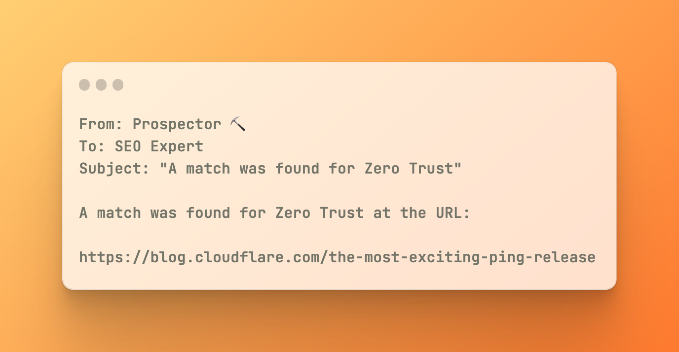
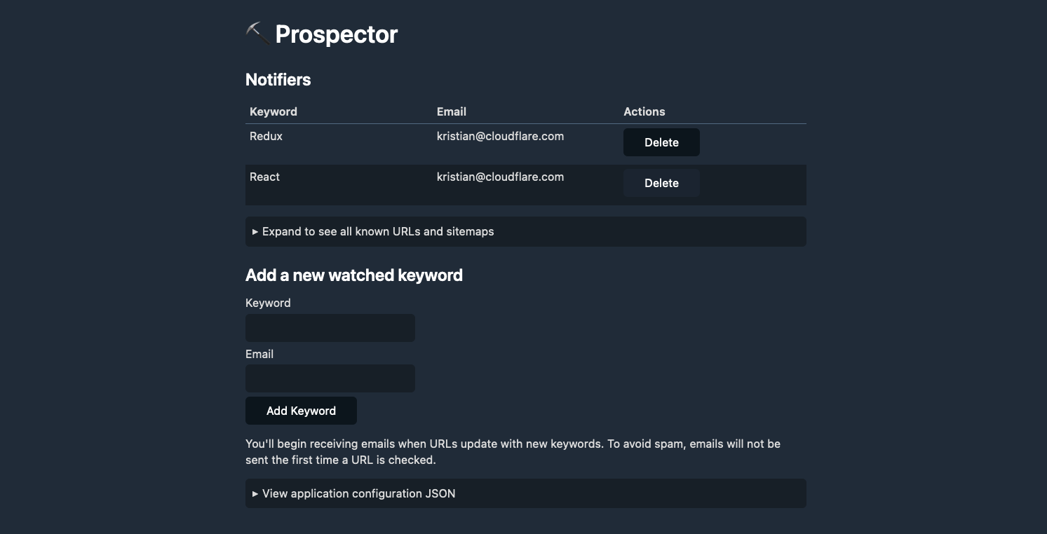
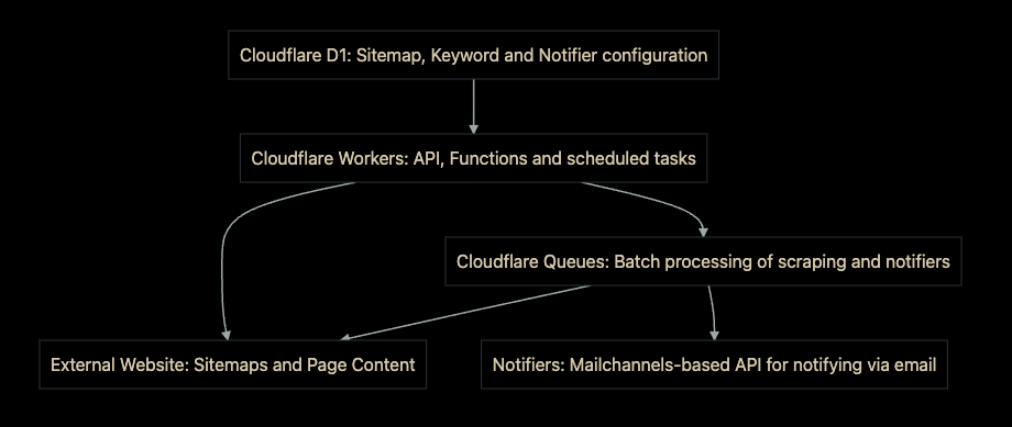
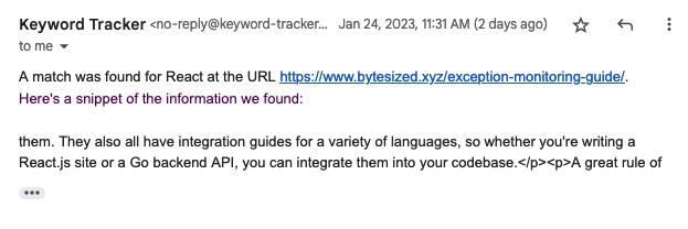


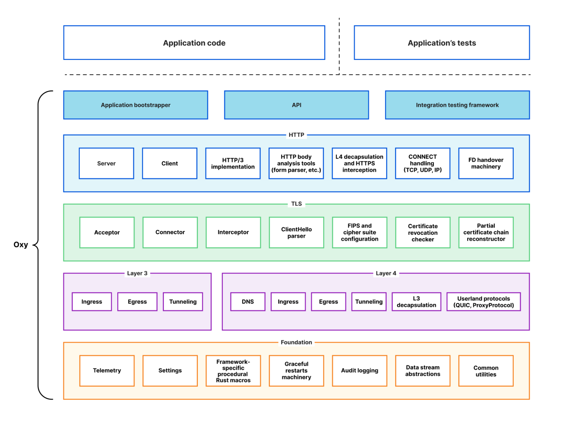
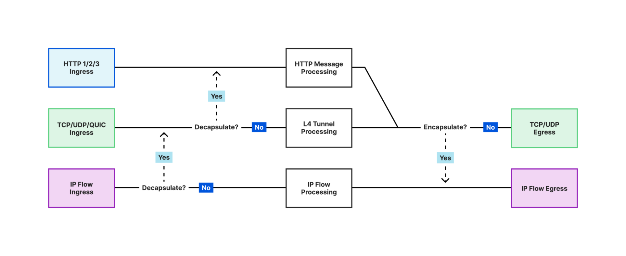
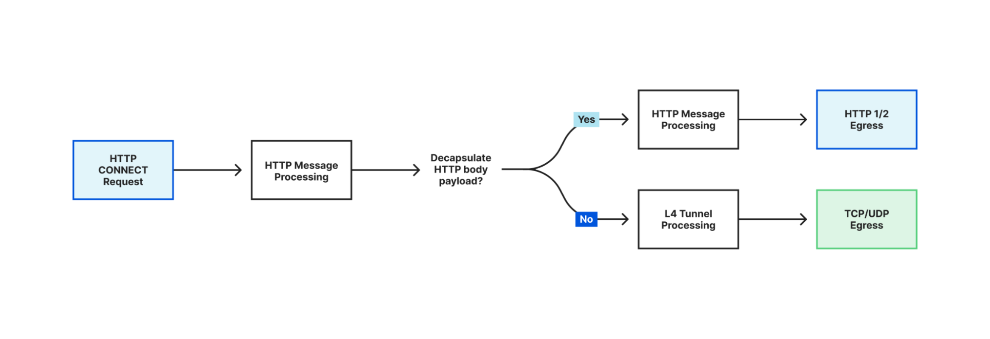


 Kachi Odoemene is an Applied Scientist at AWS AI. He builds AI/ML solutions to solve business problems for AWS customers.
 Taylor McNally is a Deep Learning Architect at Amazon Machine Learning Solutions Lab. He helps customers from various industries build solutions leveraging AI/ML on AWS. He enjoys a good cup of coffee, the outdoors, and time with his family and energetic dog.
 Austin Welch is a Data Scientist in the Amazon ML Solutions Lab. He develops custom deep learning models to help AWS public sector customers accelerate their AI and cloud adoption. In his spare time, he enjoys reading, traveling, and jiu-jitsu.


 Ajit Puthiyavettle is a Solution Architect working with enterprise clients, architecting solutions to achieve business outcomes. He is passionate about solving customer challenges with innovative solutions. His experience is with leading DevOps and security teams for enterprise and SaaS (Software as a Service) companies. Recently he is focussed on helping customers with Security, ML and HCLS workload.