Tag Archives: Analytics

Amazon OpenSearch Service Under the Hood: Multi-AZ with standby

Post Syndicated from Rohin Bhargava original https://aws.amazon.com/blogs/big-data/amazon-opensearch-service-under-the-hood-multi-az-with-standby/

Amazon OpenSearch Service recently announced Multi-AZ with standby, a new deployment option for managed clusters that enables 99.99% availability and consistent performance for business-critical workloads. With Multi-AZ with standby, clusters are resilient to infrastructure failures like hardware or networking failure. This option provides improved reliability and the added benefit of simplifying cluster configuration and management by enforcing best practices and reducing complexity.

In this post, we share how Multi-AZ with standby works under the hood to achieve high resiliency and consistent performance to meet the four 9s.

Background

One of the principles in designing highly available systems is that they need to be ready for impairments before they happen. OpenSearch is a distributed system, which runs on a cluster of instances that have different roles. In OpenSearch Service, you can deploy data nodes to store your data and respond to indexing and search requests, you can also deploy dedicated cluster manager nodes to manage and orchestrate the cluster. To provide high availability, one common approach for the cloud is to deploy infrastructure across multiple AWS Availability Zones. Even in the rare case that a full zone becomes unavailable, the available zones continue to serve traffic with replicas.

When you use OpenSearch Service, you create indexes to hold your data and specify partitioning and replication for those indexes. Each index is comprised of a set of primary shards and zero to many replicas of those shards. When you additionally use the Multi-AZ feature, OpenSearch Service ensures that primary shards and replica shards are distributed so that they’re in different Availability Zones.

When there is an impairment in an Availability Zone, the service would scale up in other Availability Zones and redistribute shards to spread out the load evenly. This approach was reactive at best. Additionally, shard redistribution during failure events causes increased resource utilization, leading to increased latencies and overloaded nodes, further impacting availability and effectively defeating the purpose of fault-tolerant, multi-AZ clusters. A more effective, statically stable cluster configuration requires provisioning infrastructure to the point where it can continue operating correctly without having to launch any new capacity or redistribute any shards even if an Availability Zone becomes impaired.

Designing for high availability

OpenSearch Service manages tens of thousands of OpenSearch clusters. We’ve gained insights into which cluster configurations like hardware (data or cluster-manager instance types) or storage (EBS volume types), shard sizes, and so on are more resilient to failures and can meet the demands of common customer workloads. Some of these configurations have been included in Multi-AZ with standby to simplify configuring the clusters. However, this alone is not enough. A key ingredient in achieving high availability is maintaining data redundancy.

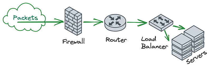
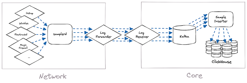
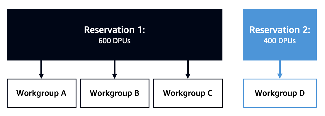
When you configure a single replica (two copies) for your indexes, the cluster can tolerate the loss of one shard (primary or replica) and still recover by copying the remaining shard. A two-replica (three copies) configuration can tolerate failure of two copies. In the case of a single replica with two copies, you can still sustain data loss. For example, you could lose data if there is a catastrophic failure in one Availability Zone for a prolonged duration, and at the same time, a node in a second zone fails. To ensure data redundancy at all times, the cluster enforces a minimum of two replicas (three copies) across all its indexes. The following diagram illustrates this architecture.

The Multi-AZ with standby feature deploys infrastructure in three Availability Zones, while keeping two zones as active and one zone as standby. The standby zone offers consistent performance even during zonal failures by ensuring same capacity at all times and by using a statically stable design without any capacity provisioning or data movements during failure. During normal operations, the active zone serves coordinator traffic for read and write requests and shard query traffic, and only replication traffic goes to the standby zone. OpenSearch uses synchronous replication protocol for write requests, which by design has zero replication lag, enabling the service to instantaneously promote a standby zone to active in the event of any failure in an active zone. This event is referred to as a zonal failover. The previously active zone is demoted to the standby mode and recovery operations to bring the state back to healthy begin.

Why zonal failover is critical but hard to do right

One or more nodes in an Availability Zone can fail due to a wide variety of reasons, like hardware failures, infrastructure failures like fiber cuts, power or thermal issues, or inter-zone or intra-zone networking problems. Read requests can be served by any of the active zones, whereas write requests need to be synchronously replicated to all copies across multiple Availability Zones. OpenSearch Service orchestrates two modes of failovers: read failovers and the write failovers.

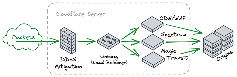
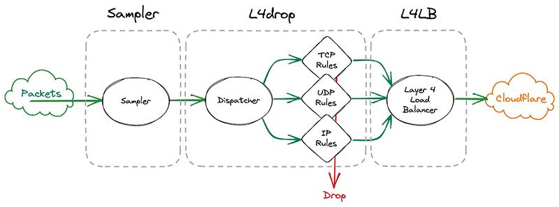
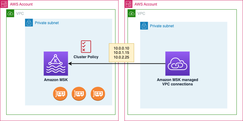
The primarily goals of read failovers are high availability and consistent performance. This requires the system to constantly monitor for faults and shift traffic away from the unhealthy nodes in the impacted zone. The system takes care of handling the failovers gracefully, allowing all in-flight requests to finish while simultaneously shifting new incoming traffic to a healthy zone. However, it’s also possible for multiple shard copies across both active zones to be unavailable in cases of two node failures or one zone plus one node failure (often referred to as double faults), which poses a risk to availability. To solve this challenge, the system uses a fail-open mechanism to serve traffic off the third zone while it may still be in a standby mode to ensure the system remains highly available. The following diagram illustrates this architecture.

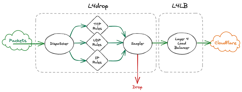
An impaired network device impacting inter-zone communication can cause write requests to significantly slow down, owing to the synchronous nature of replication. In such an event, the system orchestrates a write failover to isolate the impaired zone, cutting off all ingress and egress traffic. Although with write failovers the recovery is immediate, it results in all nodes along with its shards being taken offline. However, after the impacted zone is brought back after network recovery, shard recovery should still be able to use unchanged data from its local disk, avoiding full segment copy. Because the write failover results in the shard copy to be unavailable, we exercise write failovers with extreme caution, neither too frequently nor during transient failures.

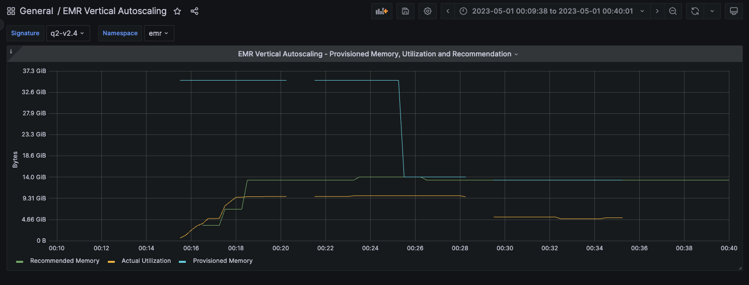
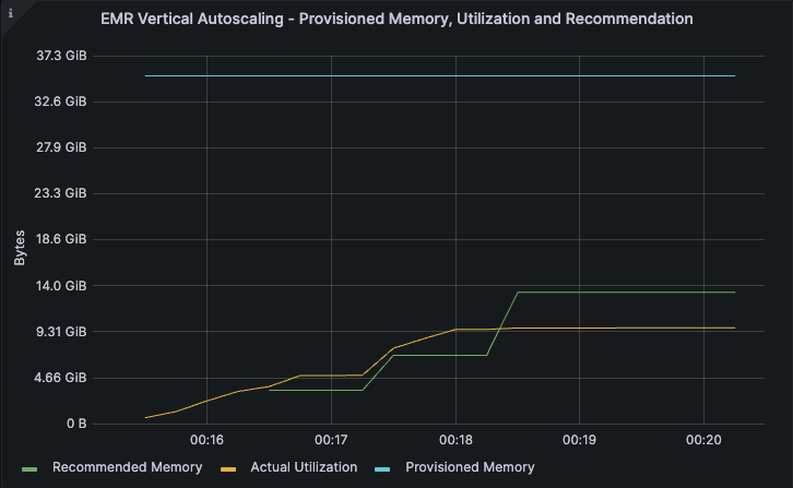
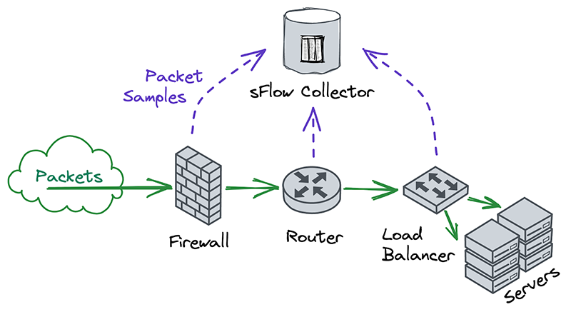
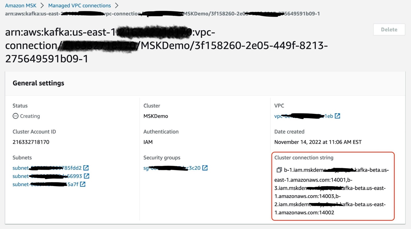
The following graph depicts that during a zonal failure, automatic read failover prevents any impact to availability.

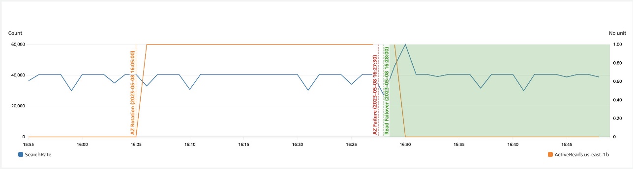
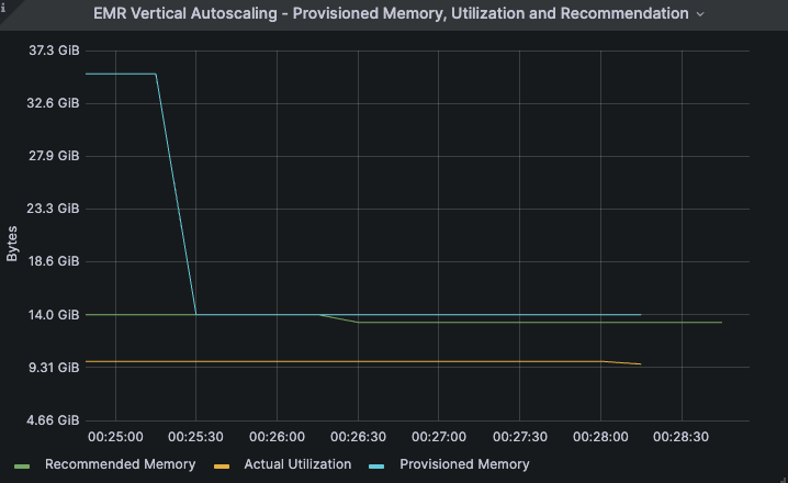
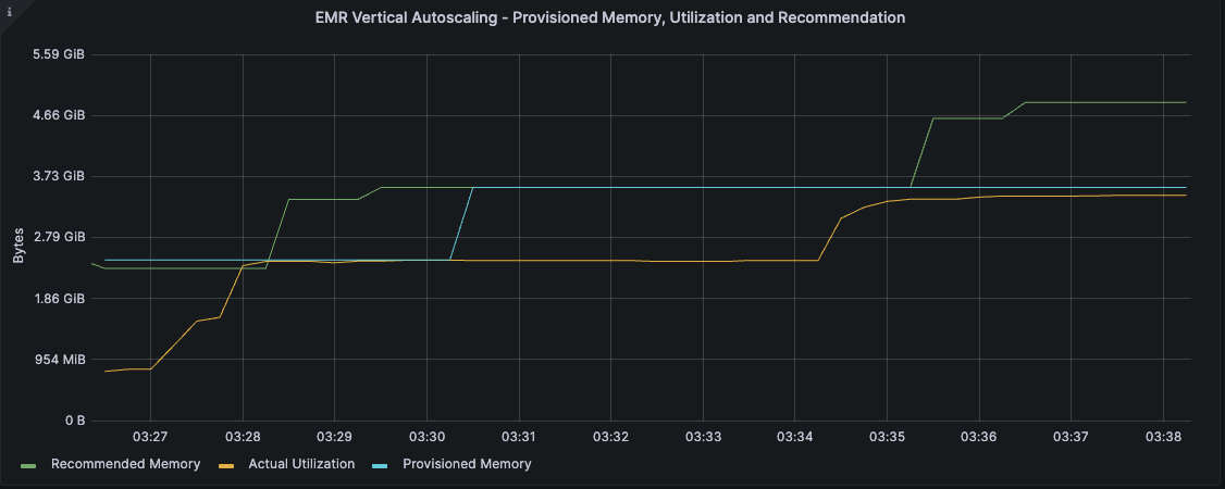
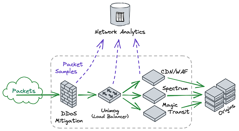
The following depicts that during a networking slowdown in a zone, write failover helps recover availability.

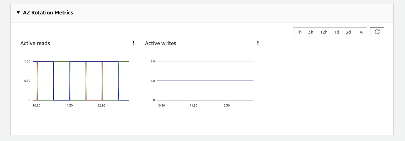
To ensure that the zonal failover mechanism is predictable (able to seamlessly shift traffic during an actual failure event), we regularly exercise failovers and keep rotating active and standby zones even during steady state. This not only verifies all network paths, ensuring we don’t hit surprises like clock skews, stale credentials, or networking issues during failover, but it also keeps gradually shifting caches to avoid cold starts on failovers, ensuring we deliver consistent performance at all times.

Improving the resiliency of the service

OpenSearch Service uses several principles and best practices to increase reliability, like automatic detection and faster recovery from failure, throttling excess requests, fail fast strategies, limiting queue sizes, quickly adapting to meet workload demands, implementing loosely coupled dependencies, continuously testing for failures, and more. We discuss a few of these methods in this section.

Automatic failure detection and recovery

All faults get monitored at a minutely granularity, across multiple sub-minutely metrics data points. Once detected, the system automatically triggers a recovery action on the impacted node. Although most classes of failures discussed so far in this post refer to binary failures where the failure is definitive, there is another kind of failure: non-binary failures, termed gray failures, whose manifestations are subtle and usually defy quick detection. Slow disk I/O is one example, which causes performance to be adversely impacted. The monitoring system detects anomalies in I/O wait times, latencies, and throughput, to detect and replace a node with slow I/O. Faster and effective detection and quick recovery is our best bet for a wide variety of infrastructure failures beyond our control.

Effective workload management in a dynamic environment

We’ve studied workload patterns that cause the system either to be overloaded with too many requests, maxing out CPU/memory, or a few rogue queries that can that either allocate huge chunks of memory or runaway queries that can exhaust multiple cores, either degrading the latencies of other critical requests or causing multiple nodes to fail due to the system’s resources running low. Some of the improvements in this direction are being done as a part of search backpressure initiatives, starting with tracking the request footprint at various checkpoints that prevents accommodating more requests and cancels the ones already running if they breach the resource limits for a sustained duration. To supplement backpressure in traffic shaping, we use admission control, which provides capabilities to reject a request at the entry point to avoid doing non-productive work (requests either time out or get cancelled) when the system is already run high on CPU and memory. Most of the workload management mechanisms have configurable knobs. No one size fits all workloads, therefore we use Auto-Tune to control them more granularly.

The cluster manager performs critical coordination tasks like metadata management and cluster formation, and orchestrates a few background operations like snapshot and shard placement. We added a task throttler to control the rate of dynamic mapping updates, snapshot tasks, and so on to prevent overwhelming it and to let critical operations run deterministically all the time. But what happens when there is no cluster manager in the cluster? The next section covers how we solved this.

Decoupling critical dependencies

In the event of cluster manager failure, searches continue as usual, but all write requests start to fail. We concluded that allowing writes in this state should still be safe as long as it doesn’t need to update the cluster metadata. This change further improves the write availability without compromising data consistency. Other service dependencies were evaluated to ensure downstream dependencies can scale as the cluster grows.

Failure mode testing

Although it’s hard to mimic all kinds of failures, we rely on AWS Fault Injection Simulator (AWS FIS) to inject common faults in the system like node failures, disk impairment, or network impairment. Testing with AWS FIS regularly in our pipelines helps us improve our detection, monitoring, and recovery times.

Contributing to open source

OpenSearch is an open-source, community-driven software. Most of the changes including the high availability design to support active and standby zones have been contributed to open source; in fact, we follow an open-source first development model. The fundamental primitive that enables zonal traffic shift and failover is based on a weighted traffic routing policy (active zones are assigned weights as 1 and standby zones are assigned weights as 0). Write failovers use the zonal decommission action, which evacuates all traffic from a given zone. Resiliency improvements for search backpressure and cluster manager task throttling are some of the ongoing efforts. If you’re excited to contribute to OpenSearch, open up a GitHub issue and let us know your thoughts.

Summary

Efforts to improve reliability is a never-ending cycle as we continue to learn and improve. With the Multi-AZ with standby feature, OpenSearch Service has integrated best practices for cluster configuration, improved workload management, and achieved four 9s of availability and consistent performance. OpenSearch Service also raised the bar by continuously verifying availability with zonal traffic rotations and automated tests via AWS FIS.

We are excited to continue our efforts into improving the reliability and fault tolerance even further and to see what new and existing solutions builders can create using OpenSearch Service. We hope this leads to a deeper understanding of the right level of availability based on the needs of your business and how this offering achieves the availability SLA. We would love to hear from you, especially about your success stories achieving high levels of availability on AWS. If you have other questions, please leave a comment.


About the authors

Bukhtawar Khan is a Principal Engineer working on Amazon OpenSearch Service. He is interested in building distributed and autonomous systems. He is a maintainer and an active contributor to OpenSearch.

Gaurav Bafna is a Senior Software Engineer working on OpenSearch at Amazon Web Services. He is fascinated about solving problems in distributed systems. He is a maintainer and an active contributor to OpenSearch.

Murali Krishna is a Senior Principal Engineer at AWS OpenSearch Service. He has built AWS OpenSearch Service and AWS CloudSearch. His areas of expertise include Information Retrieval, Large scale distributed computing, low latency real time serving systems etc. He has vast experience in designing and building web scale systems for crawling, processing, indexing and serving text and multimedia content. Prior to Amazon, he was part of Yahoo!, building crawling and indexing systems for their search products.

Ranjith Ramachandra is a Senior Engineering Manager working on Amazon OpenSearch Service. He is passionate about highly scalable distributed systems, high performance and resilient systems.

Rohin Bhargava is a Sr. Product Manager with the Amazon OpenSearch Service team. His passion at AWS is to help customers find the correct mix of AWS services to achieve success for their business goals.

Scale your AWS Glue for Apache Spark jobs with new larger worker types G.4X and G.8X

Post Syndicated from Noritaka Sekiyama original https://aws.amazon.com/blogs/big-data/scale-your-aws-glue-for-apache-spark-jobs-with-new-larger-worker-types-g-4x-and-g-8x/

Hundreds of thousands of customers use AWS Glue, a serverless data integration service, to discover, prepare, and combine data for analytics, machine learning (ML), and application development. AWS Glue for Apache Spark jobs work with your code and configuration of the number of data processing units (DPU). Each DPU provides 4 vCPU, 16 GB memory, and 64 GB disk. AWS Glue manages running Spark and adjusts workers to achieve the best price performance. For workloads such as data transforms, joins, and queries, you can use G.1X (1 DPU) and G.2X (2 DPU) workers, which offer a scalable and cost-effective way to run most jobs. With exponentially growing data sources and data lakes, customers want to run more data integration workloads, including their most demanding transforms, aggregations, joins, and queries. These workloads require higher compute, memory, and storage per worker.

Today we are pleased to announce the general availability of AWS Glue G.4X (4 DPU) and G.8X (8 DPU) workers, the next series of AWS Glue workers for the most demanding data integration workloads. G.4X and G.8X workers offer increased compute, memory, and storage, making it possible for you to vertically scale and run intensive data integration jobs, such as memory-intensive data transforms, skewed aggregations, and entity detection checks involving petabytes of data. Larger worker types not only benefit the Spark executors, but also in cases where the Spark driver needs larger capacity—for instance, because the job query plan is quite large.

This post demonstrates how AWS Glue G.4X and G.8X workers help you scale your AWS Glue for Apache Spark jobs.

G.4X and G.8X workers

AWS Glue G.4X and G.8X workers give you more compute, memory, and storage to run your most demanding jobs. G.4X workers provide 4 DPU, with 16 vCPU, 64 GB memory, and 256 GB of disk per node. G.8X workers provide 8 DPU, with 32 vCPU, 128 GB memory, and 512 GB of disk per node. You can enable G.4X and G.8X workers with a single parameter change in the API, AWS Command Line Interface (AWS CLI), or visually in AWS Glue Studio. Regardless of the worker used, all AWS Glue jobs have the same capabilities, including auto scaling and interactive job authoring via notebooks. G.4X and G.8X workers are available with AWS Glue 3.0 and 4.0.

The following table shows compute, memory, disk, and Spark configurations per worker type in AWS Glue 3.0 or later.

AWS Glue Worker Type DPU per Node vCPU Memory (GB) Disk (GB) Number of Spark Executors per Node Number of Cores per Spark Executor
G.1X 1 4 16 64 1 4
G.2X 2 8 32 128 1 8
G.4X (new) 4 16 64 256 1 16
G.8X (new) 8 32 128 512 1 32

To use G.4X and G.8X workers on an AWS Glue job, change the setting of the worker type parameter to G.4X or G.8X. In AWS Glue Studio, you can choose G 4X or G 8X under Worker type.

In the AWS API or AWS SDK, you can specify G.4X or G.8X in the WorkerType parameter. In the AWS CLI, you can use the --worker-type parameter in a create-job command.

To use G.4X and G.8X on an AWS Glue Studio notebook or interactive sessions, set G.4X or G.8X in the %worker_type magic:

Performance characteristics using the TPC-DS benchmark

In this section, we use the TPC-DS benchmark to showcase performance characteristics of the new G.4X and G.8X worker types. We used AWS Glue version 4.0 jobs.

G.2X, G.4X, and G.8X results with the same number of workers

Compared to the G.2X worker type, the G.4X worker has 2 times the DPUs and the G.8X worker has 4 times the DPUs. We ran over 100 TPC-DS queries against the 3 TB TPC-DS dataset with the same number of workers but on different worker types. The following table shows the results of the benchmark.

Worker Type Number of Workers Number of DPUs Duration (minutes) Cost at $0.44/DPU-hour ($)
G.2X 30 60 537.4 $236.46
G.4X 30 120 264.6 $232.85
G.8X 30 240 122.6 $215.78

When running jobs on the same number of workers, the new G.4X and G.8x workers achieved roughly linear vertical scalability.

G.2X, G.4X, and G.8X results with the same number of DPUs

We ran over 100 TPC-DS queries against the 10 TB TPC-DS dataset with the same number of DPUs but on different worker types. The following table shows the results of the experiments.

Worker Type Number of Workers Number of DPUs Duration (minutes) Cost at $0.44/DPU-hour ($)
G.2X 40 80 1323 $776.16
G.4X 20 80 1191 $698.72
G.8X 10 80 1190 $698.13

When running jobs on the same number of total DPUs, the job performance stayed mostly the same with new worker types.

Example: Memory-intensive transformations

Data transformations are an essential step to preprocess and structure your data into an optimal form. Bigger memory footprints are consumed in some transformations such as aggregation, join, your own custom logic using user-defined functions (UDFs), and so on. The new G.4X and G.8X workers enable you to run larger memory-intensive transformations at scale.

The following example reads large JSON files compressed in GZIP from an input Amazon Simple Storage Service (Amazon S3) location, performs groupBy, calculates groups based on K-means clustering using a Pandas UDF, then shows the results. Note that this UDF-based K-means is used just for illustration purposes; it’s recommended to use native K-means clustering for production purposes.

With G.2X workers

When an AWS Glue job runs on 12 G.2X workers (24 DPU), it failed due to a No space left on device error. On the Spark UI, the Stages tab for the failed stage shows that there were multiple failed tasks in the AWS Glue job due to the error.

The Executor tab shows failed tasks per executor.

Generally, G.2X workers can process memory-intensive workload well. This time, we used a special Pandas UDF that consumes a significant amount of memory, and it caused a failure due to a large amount of shuffle writes.

With G.8X workers

When an AWS Glue job runs on 3 G.8X workers (24 DPU), it succeeded without any failures, as shown on the Spark UI’s Jobs tab.

The Executors tab also explains that there were no failed tasks.

From this result, we observed that G.8X workers processed the same workload without failures.

Conclusion

In this post, we demonstrated how AWS Glue G.4X and G.8X workers can help you vertically scale your AWS Glue for Apache Spark jobs. G.4X and G.8X workers are available today in US East (Ohio), US East (N. Virginia), US West (Oregon), Asia Pacific (Singapore), Asia Pacific (Sydney), Asia Pacific (Tokyo), Canada (Central), Europe (Frankfurt), Europe (Ireland), and Europe (Stockholm). You can start using the new G.4X and G.8X worker types to scale your workload from today. To get started with AWS Glue, visit AWS Glue.


About the authors

Noritaka Sekiyama is a Principal Big Data Architect on the AWS Glue team. He works based in Tokyo, Japan. He is responsible for building software artifacts to help customers. In his spare time, he enjoys cycling with his road bike.

Tomohiro Tanaka is a Senior Cloud Support Engineer on the AWS Support team. He’s passionate about helping customers build data lakes using ETL workloads. In his free time, he enjoys coffee breaks with his colleagues and making coffee at home.

Chuhan LiuChuhan Liu is a Software Development Engineer on the AWS Glue team. He is passionate about building scalable distributed systems for big data processing, analytics, and management. In his spare time, he enjoys playing tennis.

Matt Su is a Senior Product Manager on the AWS Glue team. He enjoys helping customers uncover insights and make better decisions using their data with AWS Analytic services. In his spare time, he enjoys skiing and gardening.

New scatter plot options in Amazon QuickSight to visualize your data

Post Syndicated from Bhupinder Chadha original https://aws.amazon.com/blogs/big-data/new-scatter-plot-options-in-amazon-quicksight-to-visualize-your-data/

Are you looking to understand the relationships between two numerical variables? Scatter plots are a powerful visual type that allow you to identify patterns, outliers, and strength of relationships between variables. In this post, we walk you through the newly launched scatter plot features in Amazon QuickSight, which will help you take your correlation analysis to the next level.

Feature overview

The scatter plot is undoubtedly one of the most effective visualizations for correlation analysis, helping to identify patterns, outliers, and the strength of the relationship between two or three variables (using a bubble chart). We have improved the performance and versatility of our scatter plots, supporting five additional use cases. The following functionalities have been added in this release:

  • Display unaggregated values – Previously, when there was no field placed on Color, QuickSight displayed unaggregated values, and when a field was placed on Color, the metrics would be aggregated and grouped by that dimension. Now, you can choose to plot unaggregated values even if you’re using a field on Color by using the new aggregate option called None from the field menu, in addition to aggregation options like Sum, Min, and Max. If one value is set to be aggregated, the other value will be automatically set as aggregated, and the same applies to unaggregated scenarios. Mixed aggregation scenarios are not supported, meaning that one value can’t be set as aggregated while the other is unaggregated. It’s worth noting that the unaggregated scenario (the None option) is only supported for numerical values, whereas categorical values (like dates and dimensions) will only display aggregate values such as Count and Count distinct.
  • Support for an additional Label field – We’re introducing a new field well called Label alongside the existing Color field. This will allow you to color by one field and label by another, providing more flexibility in data visualization.
  • Faster load time – The load time is up to six times faster, which impacts both new and existing use cases. Upon launch, you’ll notice that scatter plots render noticeably faster, especially when dealing with larger datasets.

Explore advanced scatter plot use cases

You can choose to set both X and Y values to either aggregated or unaggregated (the None option) from the X and Y axis field menus. This will define if values will be aggregated by dimensions in the Color and Label field wells or not. To get started, add the required fields and choose the appropriate aggregation based on your use case.

Unaggregated use cases

The following screenshot shows an example of unaggregated X and Y value with Color.

The following screenshot shows an example of unaggregated X and Y with Label.

The following screenshot shows an example of unaggregated X and Y with Color and Label.

Aggregated use cases

The following screenshot shows an example of X and Y aggregated by Color.

The following screenshot shows an example of X and Y aggregated by Label.

The following screenshot shows an example of X and Y aggregated by Color and Label.

Conclusion

In summary, our enhanced scatter plots offer users greater performance and versatility, catering to a wider range of use cases than before. The ability to display unaggregated values and support for additional label fields gives users the flexibility they need to visualize the data they want. For further details, refer to Amazon QuickSight Scatterplot. Try out the new scatter plot updates and let us know your feedback in the comments section.


About the authors

Bhupinder Chadha is a senior product manager for Amazon QuickSight focused on visualization and front end experiences. He is passionate about BI, data visualization and low-code/no-code experiences. Prior to QuickSight he was the lead product manager for Inforiver, responsible for building a enterprise BI product from ground up. Bhupinder started his career in presales, followed by a small gig in consulting and then PM for xViz, an add on visualization product.

Single sign-on with Amazon Redshift Serverless with Okta using Amazon Redshift Query Editor v2 and third-party SQL clients

Post Syndicated from Maneesh Sharma original https://aws.amazon.com/blogs/big-data/single-sign-on-with-amazon-redshift-serverless-with-okta-using-amazon-redshift-query-editor-v2-and-third-party-sql-clients/

Amazon Redshift Serverless makes it easy to run and scale analytics in seconds without the need to set up and manage data warehouse clusters. With Redshift Serverless, users such as data analysts, developers, business professionals, and data scientists can get insights from data by simply loading and querying data in the data warehouse.

Customers use their preferred SQL clients to analyze their data in Redshift Serverless. They want to use an identity provider (IdP) or single sign-on (SSO) credentials to connect to Redshift Serverless to reuse existing using credentials and avoid additional user setup and configuration. When you use AWS Identity and Access Management (IAM) or IdP-based credentials to connect to a serverless data warehouse, Amazon Redshift automatically creates a database user for the end-user. You can simplify managing user privileges by using role-based access control. Admins can use a database-role mapping for SSO with the IAM roles that users are assigned to get their database privileges automatically. With this integration, organizations can simplify user management because they no longer need to create users and map them to database roles manually. You can define the mapped database roles as a principal tag for the IdP groups or IAM role, so Amazon Redshift database roles and users who are members of those IdP groups are granted to the database roles automatically.

In this post, we focus on Okta as the IdP and provide step-by-step guidance to integrate Redshift Serverless with Okta using the Amazon Redshift Query Editor V2 and with SQL clients like SQL Workbench/J. You can use this mechanism with other IdP providers such as Azure Active Directory or Ping with any applications or tools using Amazon’s JDBC/ODBC/Python driver.

Solution overview

The following diagram illustrates the authentication flow of Okta with Redshift Serverless using federated IAM roles and automatic database-role mapping.

The workflow contains the following steps:

  1. Either the user chooses an IdP app in their browser, or the SQL client initiates a user authentication request to the IdP (Okta).
  2. Upon a successful authentication, Okta submits a request to the AWS federation endpoint with a SAML assertion containing the PrincipalTags.
  3. The AWS federation endpoint validates the SAML assertion and invokes the AWS Security Token Service (AWS STS) API AssumeRoleWithSAML. The SAML assertion contains the IdP user and group information that is stored in the RedshiftDbUser and RedshiftDbRoles principal tags, respectively. Temporary IAM credentials are returned to the SQL client or, if using the Query Editor v2, the user’s browser is redirected to the Query Editor v2 console using the temporary IAM credentials.
  4. The temporary IAM credentials are used by the SQL client or Query Editor v2 to call the Redshift Serverless GetCredentials API. The API uses the principal tags to determine the user and database roles that the user belongs to. An associated database user is created if the user is signing in for the first time and is granted the matching database roles automatically. A temporary password is returned to the SQL client.
  5. Using the database user and temporary password, the SQL client or Query Editor v2 connects to Redshift Serverless. Upon login, the user is authorized based on the Amazon Redshift database roles that were assigned in Step 4.

To set up the solution, we complete the following steps:

  1. Set up your Okta application:
    • Create Okta users.
    • Create groups and assign groups to users.
    • Create the Okta SAML application.
    • Collect Okta information.
  2. Set up AWS configuration:
    • Create the IAM IdP.
    • Create the IAM role and policy.
  3. Configure Redshift Serverless role-based access.
  4. Federate to Redshift Serverless using the Query Editor V2.
  5. Configure the SQL client (for this post, we use SQL Workbench/J).
  6. Optionally, implement MFA with SQL Client and Query Editor V2.

Prerequisites

You need the following prerequisites to set up this solution:

Set up Okta application

In this section, we provide the steps to configure your Okta application.

Create Okta users

To create your Okta users, complete the following steps:

  1. Sign in to your Okta organization as a user with administrative privileges.
  2. On the admin console, under Directory in the navigation pane, choose People.
  3. Choose Add person.
  4. For First Name, enter the user’s first name.
  5. For Last Name, enter the user’s last name.
  6. For Username, enter the user’s user name in email format.
  7. Select I will set password and enter a password.
  8. Optionally, deselect User must change password on first login if you don’t want the user to change their password when they first sign in. Choose Save.

Create groups and assign groups to users

To create your groups and assign them to users, complete the following steps:

  1. Sign in to your Okta organization as a user with administrative privileges.
  2. On the admin console, under Directory in the navigation pane, choose Groups.
  3. Choose Add group.
  4. Enter a group name and choose Save.
  5. Choose the recently created group and then choose Assign people.
  6. Choose the plus sign and then choose Done.
  7. Repeat Steps 1–6 to add more groups.

In this post, we create two groups: sales and finance.

Create an Okta SAML application

To create your Okta SAML application, complete the following steps:

  1. Sign in to your Okta organization as a user with administrative privileges.
  2. On the admin console, under Applications in the navigation pane, choose Applications.
  3. Choose Create App Integration.
  4. Select SAML 2.0 as the sign-in method and choose Next.
  5. Enter a name for your app integration (for example, redshift_app) and choose Next.
  6. Enter following values in the app and leave the rest as is:
    • For Single Sign On URL, enter https://signin.aws.amazon.com/saml.
    • For Audience URI (SP Entity ID), enter urn:amazon:webservices.
    • For Name ID format, enter EmailAddress.
  7. Choose Next.
  8. Choose I’m an Okta customer adding an internal app followed by This is an internal app that we have created.
  9. Choose Finish.
  10. Choose Assignments and then choose Assign.
  11. Choose Assign to groups and then select Assign next to the groups that you want to add.
  12. Choose Done.

Set up Okta advanced configuration

After you create the custom SAML app, complete the following steps:

  1. On the admin console, navigate to General and choose Edit under SAML settings.
  2. Choose Next.
  3. Set Default Relay State to the Query Editor V2 URL, using the format https://<region>.console.aws.amazon.com/sqlworkbench/home. For this post, we use https://us-west-2.console.aws.amazon.com/sqlworkbench/home.
  4. Under Attribute Statements (optional), add the following properties:
    • Provide the IAM role and IdP in comma-separated format using the Role attribute. You’ll create this same IAM role and IdP in a later step when setting up AWS configuration.
    • Set user.login for RoleSessionName. This is used as an identifier for the temporary credentials that are issued when the role is assumed.
    • Set the DB roles using PrincipalTag:RedshiftDbRoles. This uses the Okta groups to fill the principal tags and map them automatically with the Amazon Redshift database roles. Its value must be a colon-separated list in the format role1:role2.
    • Set user.login for PrincipalTag:RedshiftDbUser. This uses the user name in the directory. This is a required tag and defines the database user that is used by Query Editor V2.
    • Set the transitive keys using TransitiveTagKeys. This prevents users from changing the session tags in case of role chaining.

The preceding tags are forwarded to the GetCredentials API to get temporary credentials for your Redshift Serverless instance and map automatically with Amazon Redshift database roles. The following table summarizes their attribute statements configuration.

Name Name Format Format Example
https://aws.amazon.com/SAML/Attributes/Role Unspecified arn:aws:iam::<yourAWSAccountID>:role/role-name,arn:aws:iam:: <yourAWSAccountID>:saml-provider/provider-name arn:aws:iam::112034567890:role/oktarole,arn:aws:iam::112034567890:saml-provider/oktaidp
https://aws.amazon.com/SAML/Attributes/RoleSessionName Unspecified user.login user.login
https://aws.amazon.com/SAML/Attributes/PrincipalTag:RedshiftDbRoles Unspecified String.join(":", isMemberOfGroupName("group1") ? 'group1' : '', isMemberOfGroupName("group2") ? 'group2' : '') String.join(":", isMemberOfGroupName("sales") ? 'sales' : '', isMemberOfGroupName("finance") ? 'finance' : '')
https://aws.amazon.com/SAML/Attributes/PrincipalTag:RedshiftDbUser Unspecified user.login user.login
https://aws.amazon.com/SAML/Attributes/TransitiveTagKeys Unspecified Arrays.flatten("RedshiftDbUser", "RedshiftDbRoles") Arrays.flatten("RedshiftDbUser", "RedshiftDbRoles")
  1. After you add the attribute claims, choose Next followed by Finish.

Your attributes should be in similar format as shown in the following screenshot.

Collect Okta information

To gather your Okta information, complete the following steps:

  1. On the Sign On tab, choose View SAML setup instructions.
  2. For Identity Provider Single Sign-on URL, Use this URL when connecting with any third-party SQL client such as SQL Workbench/J.
  3. Use the IdP metadata in block 4 and save the metadata file in .xml format (for example, metadata.xml).

Set up AWS configuration

In this section, we provide the steps to configure your IAM resources.

Create the IAM IdP

To create your IAM IdP, complete the following steps:

  1. On the IAM console, under Access management in the navigation pane, choose Identity providers.
  2. Choose Add provider.
  3. For Provider type¸ select SAML.
  4. For Provider name¸ enter a name.
  5. Choose Choose file and upload the metadata file (.xml) you downloaded earlier.
  6. Choose Add provider.

Create the IAM Amazon Redshift access policy

To create your IAM policy, complete the following steps:

  1. On the IAM console, choose Policies.
  2. Choose Create policy.
  3. On the Create policy page, choose the JSON tab.
  4. For the policy, enter the JSON in following format:
    {
        "Version": "2012-10-17",
        "Statement": [
            {
                "Sid": "VisualEditor0",
                "Effect": "Allow",
                "Action": "redshift-serverless:GetCredentials",
                "Resource": "<Workgroup ARN>"
            },
            {
                "Sid": "VisualEditor1",
                "Effect": "Allow",
                "Action": "redshift-serverless:ListWorkgroups",
                "Resource": "*"
            }
        ]
    }

The workgroup ARN is available on the Redshift Serverless workgroup configuration page.

The following example policy includes only a single Redshift Serverless workgroup; you can modify the policy to include multiple workgroups in the Resource section:

{
    "Version": "2012-10-17",
    "Statement": [
        {
            "Sid": "VisualEditor0",
            "Effect": "Allow",
            "Action": "redshift-serverless:GetCredentials",
            "Resource": "arn:aws:redshift-serverless:us-west-2:123456789012:workgroup/4a4f12vc-123b-2d99-fd34-a12345a1e87f"
        },
        {
            "Sid": "VisualEditor1",
            "Effect": "Allow",
            "Action": "redshift-serverless:ListWorkgroups",
            "Resource": "*"
        }
    ]
}

  1. Choose Next: Tags.
  2. Choose Next: Review.
  3. In the Review policy section, for Name, enter the name of your policy; for example, OktaRedshiftPolicy.
  4. For Description, you can optionally enter a brief description of what the policy does.
  5. Choose Create policy.

Create the IAM role

To create your IAM role, complete the following steps:

  1. On the IAM console, choose Roles in the navigation pane.
  2. Choose Create role.
  3. For Trusted entity type, select SAML 2.0 federation.
  4. For SAML 2.0-based provider, choose the IdP you created earlier.
  5. Select Allow programmatic and AWS Management Console access.
  6. Choose Next.
  7. Choose the policy you created earlier.
  8. Also, add the policy AmazonRedshiftQueryEditorV2ReadSharing.
  9. Choose Next.
  10. In the Review section, for Role Name, enter the name of your role; for example, oktarole.
  11. For Description, you can optionally enter a brief description of what the role does.
  12. Choose Create role.
  13. Navigate to the role that you just created and choose Trust Relationships.
  14. Choose Edit trust policy and choose TagSession under Add actions for STS.

When using session tags, trust policies for all roles connected to the IdP passing tags must have the sts:TagSession permission. For roles without this permission in the trust policy, the AssumeRole operation fails.

  1. Choose Update policy.

The following screenshot shows the role permissions.

The following screenshot shows the trust relationships.

Update the advanced Okta Role Attribute

Complete the following steps:

  1. Switch back to Okta.com.
  2. Navigate to the application which you created earlier.
  3. Navigate to General and click Edit under SAML settings.
  4. Under Attribute Statements (optional), update the value for the attribute – https://aws.amazon.com/SAML/Attributes/Role, using the actual role and identity provider arn values from the above step. For example, arn:aws:iam::123456789012:role/oktarole,arn:aws:iam::123456789012:saml-provider/oktaidp.

Configure Redshift Serverless role-based access

In this step, we create database roles in Amazon Redshift based on the groups that you created in Okta. Make sure the role name matches with the Okta Group name.

Amazon Redshift roles simplify managing privileges required for your end-users. In this post, we create two database roles, sales and finance, and grant them access to query tables with sales and finance data, respectively. You can download this sample SQL Notebook and import into Redshift Query Editor v2 to run all cells in the notebook used in this example. Alternatively, you can copy and enter the SQL into your SQL client.

The following is the syntax to create a role in Redshift Serverless:

create role <IdP groupname>;

For example:

create role sales;
create role finance;

Create the sales and finance database schema:

create schema sales_schema;
create schema finance_schema;

Create the tables:

CREATE TABLE IF NOT EXISTS finance_schema.revenue
(
account INTEGER   ENCODE az64
,customer VARCHAR(20)   ENCODE lzo
,salesamt NUMERIC(18,0)   ENCODE az64
)
DISTSTYLE AUTO
;

insert into finance_schema.revenue values (10001, 'ABC Company', 12000);
insert into finance_schema.revenue values (10002, 'Tech Logistics', 175400);
insert into finance_schema.revenue values (10003, 'XYZ Industry', 24355);
insert into finance_schema.revenue values (10004, 'The tax experts', 186577);

CREATE TABLE IF NOT EXISTS sales_schema.store_sales
(
ID INTEGER   ENCODE az64,
Product varchar(20),
Sales_Amount INTEGER   ENCODE az64
)
DISTSTYLE AUTO
;

Insert into sales_schema.store_sales values (1,'product1',1000);
Insert into sales_schema.store_sales values (2,'product2',2000);
Insert into sales_schema.store_sales values (3,'product3',3000);
Insert into sales_schema.store_sales values (4,'product4',4000);

The following is the syntax to grant permission to the Redshift Serverless role:

GRANT { { SELECT | INSERT | UPDATE | DELETE | DROP | REFERENCES } [,...]| ALL [ PRIVILEGES ] } ON { [ TABLE ] table_name [, ...] | ALL TABLES IN SCHEMA schema_name [, ...] } TO role <IdP groupname>;

Grant relevant permission to the role as per your requirements. In the following example, we grant full permission to the role sales on sales_schema and only select permission on finance_schema to the role finance:

grant usage on schema sales_schema to role sales;
grant select on all tables in schema sales_schema to role sales;

grant usage on schema finance_schema to role finance;
grant select on all tables in schema finance_schema to role finance;

Federate to Redshift Serverless using Query Editor V2

The RedshiftDbRoles principal tag and DBGroups are both mechanisms that can be used to integrate with an IdP. However, federating with the RedshiftDbRoles principal has some clear advantages when it comes to connecting with an IdP because it provides automatic mapping between IdP groups and Amazon Redshift database roles. Overall, RedshiftDbRoles is more flexible, easier to manage, and more secure, making it the better option for integrating Amazon Redshift with your IdP.

Now you’re ready to connect to Redshift Serverless using the Query Editor V2 and federated login:

  1. Use the SSO URL you collected earlier and log in to your Okta account with your user credentials. For this demo, we log in with user Ethan.
  2. In the Query Editor v2, choose your Redshift Serverless instance (right-click) and choose Create connection.
  3. For Authentication, select Federated user.
  4. For Database, enter the database name you want to connect to.
  5. Choose Create Connection.

User Ethan will be able to access sales_schema tables. If Ethan tries to access the tables in finance_schema, he will get a permission denied error.

Configure the SQL client (SQL Workbench/J)

To set up SQL Workbench/J, complete the following steps:

  1. Create a new connection in SQL Workbench/J and choose Redshift Serverless as the driver.
  2. Choose Manage drivers and add all the files from the downloaded AWS JDBC driver pack .zip file (remember to unzip the .zip file).
  3. For Username and Password, enter the values that you set in Okta.
  4. Capture the values for app_id, app_name, and idp_host from the Okta app embed link, which can be found on the General tab of your application.
  5. Set the following extended properties:
    • For app_id, enter the value from app embed link (for example, 0oa8p1o1RptSabT9abd0/avc8k7abc32lL4izh3b8).
    • For app_name, enter the value from app embed link (for example, dev-123456_redshift_app_2).
    • For idp_host, enter the value from app embed link (for example, dev-123456.okta.com).
    • For plugin_name, enter com.amazon.redshift.plugin.OktaCredentialsProvider. The following screenshot shows the SQL Workbench/J extended properties.

      1. Choose OK.
      2. Choose Test from SQL Workbench/J to test the connection.
      3. When the connection is successful, choose OK.
      4. Choose OK to sign in with the users created.

User Ethan will be able to access the sales_schema tables. If Ethan tries to access the tables in the finance_schema, he will get a permission denied error.

Congratulations! You have federated with Redshift Serverless and Okta with SQL Workbench/J using RedshiftDbRoles.

[Optional] Implement MFA with SQL Client and Query Editor V2

Implementing MFA poses an additional challenge because the nature of multi-factor authentication is an asynchronous process between initiating the login (the first factor) and completing the login (the second factor). The SAML response will be returned to the appropriate listener in each scenario; the SQL Client or the AWS console in the case of QEV2. Depending on which login options you will be giving your users, you may need an additional Okta application. See below for the different scenarios:

  1. If you are ONLY using QEV2 and not using any other SQL client, then you can use MFA with Query Editor V2 with the above application. There are no changes required in the custom SAML application which we have created above.
  2. If you are NOT using QEV2 and only using third party SQL client (SQL Workbench/J etc), then you need to modify the above custom SAML app as mentioned below.
  3. If you want to use QEV2 and third-party SQL Client with MFA, then you need create an additional custom SAML app as mentioned below.

Prerequisites for MFA

Each identity provider (IdP) has step for enabling and managing MFA for your users. In the case of Okta, see the following guides on how to enable MFA using the Okta Verify application and by defining an authentication policy.

Steps to create/update SAML application which supports MFA for a SQL Client

  1. If creating a second app, follow all the steps which are described under section 1 (Create Okta SAML application).
  2. Open the custom SAML app and select General.
  3. Select Edit under SAML settings
  4. Click Next in General Settings
  5. Under General, update the Single sign-on URL to http://localhost:7890/redshift/
  6. Select Next followed by Finish.

Below is the screenshot from the MFA App after making above changes:

Configure SQL Client for MFA

To set up SQL Workbench/J, complete the following steps:

  1. Follow all the steps which are described under (Configure the SQL client (SQL Workbench/J))
  2. Modify your connection updating the extended properties:
    • login_url – Get the Single Sign-on URL as shown in section -Collect Okta information. (For example, https://dev-123456.okta.com/app/dev-123456_redshiftapp_2/abc8p6o5psS6xUhBJ517/sso/saml)
    • plugin_name – com.amazon.redshift.plugin.BrowserSamlCredentialsProvider
  3. Choose OK
  4. Choose OK from SQL Workbench/J. You’re redirected to the browser to sign in with your Okta credentials.
  5. After that, you will get prompt for MFA. Choose either Enter a code or Get a push notification.
  6. Once authentication is successful, log in to be redirected to a page showing the connection as successful.
  7. With this connection profile, run the following query to return federated user name.

Troubleshooting

If your connection didn’t work, consider the following:

  • Enable logging in the driver. For instructions, see Configure logging.
  • Make sure to use the latest Amazon Redshift JDBC driver version.
  • If you’re getting errors while setting up the application on Okta, make sure you have admin access.
  • If you can authenticate via the SQL client but get a permission issue or can’t see objects, grant the relevant permission to the role, as detailed earlier in this post.

Clean up

When you’re done testing the solution, clean up the resources to avoid incurring future charges:

  1. Delete the Redshift Serverless instance by deleting both the workgroup and the namespace.
  2. Delete the IAM roles, IAM IdPs, and IAM policies.

Conclusion

In this post, we provided step-by-step instructions to integrate Redshift Serverless with Okta using the Amazon Redshift Query Editor V2 and SQL Workbench/J with the help of federated IAM roles and automatic database-role mapping. You can use a similar setup with any other SQL client (such as DBeaver or DataGrip) or business intelligence tool (such as Tableau Desktop). We also showed how Okta group membership is mapped automatically with Redshift Serverless roles to use role-based authentication seamlessly.

For more information about Redshift Serverless single sign-on using database roles, see Defining database roles to grant to federated users in Amazon Redshift Serverless.


About the Authors

Maneesh Sharma is a Senior Database Engineer at AWS with more than a decade of experience designing and implementing large-scale data warehouse and analytics solutions. He collaborates with various Amazon Redshift Partners and customers to drive better integration.

Debu-PandaDebu Panda is a Senior Manager, Product Management at AWS. He is an industry leader in analytics, application platform, and database technologies, and has more than 25 years of experience in the IT world.

Mohamed ShaabanMohamed Shaaban is a Senior Software Engineer in Amazon Redshift and is based in Berlin, Germany. He has over 12 years of experience in the software engineering. He is passionate about cloud services and building solutions that delight customers. Outside of work, he is an amateur photographer who loves to explore and capture unique moments.

Rajiv Gupta is Sr. Manager of Analytics Specialist Solutions Architects based out of Irvine, CA. He has 20+ years of experience building and managing teams who build data warehouse and business intelligence solutions.

Amol Mhatre is a Database Engineer in Amazon Redshift and works on Customer & Partner engagements. Prior to Amazon, he has worked on multiple projects involving Database & ERP implementations.

Ning Di is a Software Development Engineer at Amazon Redshift, driven by a genuine passion for exploring all aspects of technology.

Harsha Kesapragada is a Software Development Engineer for Amazon Redshift with a passion to build scalable and secure systems. In the past few years, he has been working on Redshift Datasharing, Security and Redshift Serverless.

How Encored Technologies built serverless event-driven data pipelines with AWS

Post Syndicated from Younggu Yun original https://aws.amazon.com/blogs/big-data/how-encored-technologies-built-serverless-event-driven-data-pipelines-with-aws/

This post is a guest post co-written with SeonJeong Lee, JaeRyun Yim, and HyeonSeok Yang from Encored Technologies.

Encored Technologies (Encored) is an energy IT company in Korea that helps their customers generate higher revenue and reduce operational costs in renewable energy industries by providing various AI-based solutions. Encored develops machine learning (ML) applications predicting and optimizing various energy-related processes, and their key initiative is to predict the amount of power generated at renewable energy power plants.

In this post, we share how Encored runs data engineering pipelines for containerized ML applications on AWS and how they use AWS Lambda to achieve performance improvement, cost reduction, and operational efficiency. We also demonstrate how to use AWS services to ingest and process GRIB (GRIdded Binary) format data, which is a file format commonly used in meteorology to store and exchange weather and climate data in a compressed binary form. It allows for efficient data storage and transmission, as well as easy manipulation of the data using specialized software.

Business and technical challenge

Encored is expanding their business into multiple countries to provide power trading services for end customers. The amount of data and the number of power plants they need to collect data are rapidly increasing over time. For example, the volume of data required for training one of the ML models is more than 200 TB. To meet the growing requirements of the business, the data science and platform team needed to speed up the process of delivering model outputs. As a solution, Encored aimed to migrate existing data and run ML applications in the AWS Cloud environment to efficiently process a scalable and robust end-to-end data and ML pipeline.

Solution overview

The primary objective of the solution is to develop an optimized data ingestion pipeline that addresses the scaling challenges related to data ingestion. During its previous deployment in an on-premises environment, the time taken to process data from ingestion to preparing the training dataset exceeded the required service level agreement (SLA). One of the input datasets required for ML models is weather data supplied by the Korea Meteorological Administration (KMA). In order to use the GRIB datasets for the ML models, Encored needed to prepare the raw data to make it suitable for building and training ML models. The first step was to convert GRIB to the Parquet file format.

Encored used Lambda to run an existing data ingestion pipeline built in a Linux-based container image. Lambda is a compute service that lets you run code without provisioning or managing servers. Lambda runs your code on a high-availability compute infrastructure and performs all of the administration of the compute resources, including server and operating system maintenance, capacity provisioning and automatic scaling, and logging. AWS Lambda is triggered to ingest and process GRIB data files when they are uploaded to Amazon Simple Storage Service (Amazon S3). Once the files are processed, they are stored in Parquet format in the other S3 bucket. Encored receives GRIB files throughout the day, and whenever new files arrive, an AWS Lambda function runs a container image registered in Amazon Elastic Container Registry (ECR). This event-based pipeline triggers a customized data pipeline that is packaged in a container-based solution. Leveraging Amazon AWS Lambda, this solution is cost-effective, scalable, and high-performing.Encored uses Python as their preferred language.

The following diagram illustrates the solution architecture.

Lambda-data-pipeline

For data-intensive tasks such as extract, transform, and load (ETL) jobs and ML inference, Lambda is an ideal solution because it offers several key benefits, including rapid scaling to meet demand, automatic scaling to zero when not in use, and S3 event triggers that can initiate actions in response to object-created events. All this contributes to building a scalable and cost-effective data event-driven pipeline. In addition to these benefits, Lambda allows you to configure ephemeral storage (/tmp) between 512–10,240 MB. Encored used this storage for their data application when reading or writing data, enabling them to optimize performance and cost-effectiveness. Furthermore, Lambda’s pay-per-use pricing model means that users only pay for the compute time in use, making it a cost-effective solution for a wide range of use cases.

Prerequisites

For this walkthrough, you should have the following:

Build your application required for your Docker image

The first step is to develop an application that can ingest and process files. This application reads the bucket name and object key passed from a trigger added to Lambda function. The processing logic involves three parts: downloading the file from Amazon S3 into ephemeral storage (/tmp), parsing the GRIB formatted data, and saving the parsed data to Parquet format.

The customer has a Python script (for example, app.py) that performs these tasks as follows:

import os
import tempfile
import boto3
import numpy as np
import pandas as pd
import pygrib

s3_client = boto3.client('s3')
def handler(event, context):
    try:
        # Get trigger file name
        bucket_name = event["Records"][0]["s3"]["bucket"]["name"]
        s3_file_name = event["Records"][0]["s3"]["object"]["key"]

        # Handle temp files: all temp objects are deleted when the with-clause is closed
        with tempfile.NamedTemporaryFile(delete=True) as tmp_file:
            # Step1> Download file from s3 into temp area
            s3_file_basename = os.path.basename(s3_file_name)
            s3_file_dirname = os.path.dirname(s3_file_name)
            local_filename = tmp_file.name
            s3_client.download_file(
                Bucket=bucket_name,
                Key=f"{s3_file_dirname}/{s3_file_basename}",
                Filename=local_filename
            )

            # Step2> Parse – GRIB2 
            grbs = pygrib.open(local_filename)
            list_of_name = []
            list_of_values = []
            for grb in grbs:
                list_of_name.append(grb.name)
                list_of_values.append(grb.values)
            _, lat, lon = grb.data()
            list_of_name += ["lat", "lon"]
            list_of_values += [lat, lon]
            grbs.close()

            dat = pd.DataFrame(
                np.transpose(np.stack(list_of_values).reshape(len(list_of_values), -1)),
                columns=list_of_name,
            )

        # Step3> To Parquet
        s3_dest_uri = S3path
        dat.to_parquet(s3_dest_uri, compression="snappy")

    except Exception as err:
        print(err)

Prepare a Docker file

The second step is to create a Docker image using an AWS base image. To achieve this, you can create a new Dockerfile using a text editor on your local machine. This Dockerfile should contain two environment variables:

  • LAMBDA_TASK_ROOT=/var/task
  • LAMBDA_RUNTIME_DIR=/var/runtime

It’s important to install any dependencies under the ${LAMBDA_TASK_ROOT} directory alongside the function handler to ensure that the Lambda runtime can locate them when the function is invoked. Refer to the available Lambda base images for custom runtime for more information.

FROM public.ecr.aws/lambda/python:3.8

# Install the function's dependencies using file requirements.txt
# from your project folder.

COPY requirements.txt  .
RUN pip3 install -r requirements.txt --target "${LAMBDA_TASK_ROOT}"

# Copy function code
COPY app.py ${LAMBDA_TASK_ROOT}

# Set the CMD to your handler (could also be done as a parameter override outside of the Dockerfile)
CMD [ "app.handler" ]

Build a Docker image

The third step is to build your Docker image using the docker build command. When running this command, make sure to enter a name for the image. For example:

docker build -t process-grib .

In this example, the name of the image is process-grib. You can choose any name you like for your Docker image.

Upload the image to the Amazon ECR repository

Your container image needs to reside in an Amazon Elastic Container Registry (Amazon ECR) repository. Amazon ECR is a fully managed container registry offering high-performance hosting, so you can reliably deploy application images and artifacts anywhere. For instructions on creating an ECR repository, refer to Creating a private repository.

The first step is to authenticate the Docker CLI to your ECR registry as follows:

aws ecr get-login-password --region ap-northeast-2 | docker login --username AWS --password-stdin 123456789012.dkr.ecr.ap-northeast-2.amazonaws.com 

The second step is to tag your image to match your repository name, and deploy the image to Amazon ECR using the docker push command:

docker tag  hello-world:latest 123456789012.dkr.ecr. ap-northeast-2.amazonaws.com/hello-world:latest
docker push 123456789012.dkr.ecr. ap-northeast-2.amazonaws.com/hello-world:latest     

Deploy Lambda functions as container images

To create your Lambda function, complete the following steps:

  1. On the Lambda console, choose Functions in the navigation pane.
  2. Choose Create function.
  3. Choose the Container image option.
  4. For Function name, enter a name.
  5. For Container image URI, provide a container image. You can enter the ECR image URI or browse for the ECR image.
  6. Under Container image overrides, you can override configuration settings such as the entry point or working directory that are included in the Dockerfile.
  7. Under Permissions, expand Change default execution role.
  8. Choose to create a new role or use an existing role.
  9. Choose Create function.

Key considerations

To handle a large amount of data concurrently and quickly, Encored needed to store GRIB formatted files in the ephemeral storage (/tmp) that comes with Lambda. To achieve this requirement, Encored used tempfile.NamedTemporaryFile, which allows users to create temporary files easily that are deleted when no longer needed. With Lambda, you can configure ephemeral storage between 512 MB–10,240 MB for reading or writing data, allowing you to run ETL jobs, ML inference, or other data-intensive workloads.

Business outcome

Hyoseop Lee (CTO at Encored Technologies) said, “Encored has experienced positive outcomes since migrating to AWS Cloud. Initially, there was a perception that running workloads on AWS would be more expensive than using an on-premises environment. However, we discovered that this was not the case once we started running our applications on AWS. One of the most fascinating aspects of AWS services is the flexible architecture options it provides for processing, storing, and accessing large volumes of data that are only required infrequently.”

Conclusion

In this post, we covered how Encored built serverless data pipelines with Lambda and Amazon ECR to achieve performance improvement, cost reduction, and operational efficiency.

Encored successfully built an architecture that will support their global expansion and enhance technical capabilities through AWS services and the AWS Data Lab program. Based on the architecture and various internal datasets Encored has consolidated and curated, Encored plans to provide renewable energy forecasting and energy trading services.

Thanks for reading this post and hopefully you found it useful. To accelerate your digital transformation with ML, AWS is available to support you by providing prescriptive architectural guidance on a particular use case, sharing best practices, and removing technical roadblocks. You’ll leave the engagement with an architecture or working prototype that is custom fit to your needs, a path to production, and deeper knowledge of AWS services. Please contact your AWS Account Manager or Solutions Architect to get started. If you don’t have an AWS Account Manager, please contact Sales.

To learn more about ML inference use cases with Lambda, check out the following blog posts:

These resources will provide you with valuable insights and practical examples of how to use Lambda for ML inference.


About the Authors

leeSeonJeong Lee is the Head of Algorithms at Encored. She is a data practitioner who finds peace of mind from beautiful codes and formulas.

yimJaeRyun Yim is a Senior Data Scientist at Encored. He is striving to improve both work and life by focusing on simplicity and essence in my work.

yangHyeonSeok Yang is the platform team lead at Encored. He always strives to work with passion and spirit to keep challenging like a junior developer, and become a role model for others.

youngguYounggu Yun works at AWS Data Lab in Korea. His role involves helping customers across the APAC region meet their business objectives and overcome technical challenges by providing prescriptive architectural guidance, sharing best practices, and building innovative solutions together.

Improve reliability and reduce costs of your Apache Spark workloads with vertical autoscaling on Amazon EMR on EKS

Post Syndicated from Rajkishan Gunasekaran original https://aws.amazon.com/blogs/big-data/improve-reliability-and-reduce-costs-of-your-apache-spark-workloads-with-vertical-autoscaling-on-amazon-emr-on-eks/

Amazon EMR on Amazon EKS is a deployment option offered by Amazon EMR that enables you to run Apache Spark applications on Amazon Elastic Kubernetes Service (Amazon EKS) in a cost-effective manner. It uses the EMR runtime for Apache Spark to increase performance so that your jobs run faster and cost less.

Apache Spark allows you to configure the amount of Memory and vCPU cores that a job will utilize. However, tuning these values is a manual process that can be complex and ripe with pitfalls. For example, allocating too little memory can result in out-of-memory exceptions and poor job reliability. On the other hand, too much can result in over-spending on idle resources, poor cluster utilization and high costs. Moreover, it’s hard to right-size these settings for some use cases such as interactive analytics due to lack of visibility into future requirements. In the case of recurring jobs, keeping these settings up to date taking into account changing load patterns (due to external seasonal factors for instance) remains a challenge.

To address this, Amazon EMR on EKS has recently announced support for vertical autoscaling, a feature that uses the Kubernetes Vertical Pod Autoscaler (VPA) to automatically tune the memory and CPU resources of EMR Spark applications to adapt to the needs of the provided workload, simplifying the process of tuning resources and optimizing costs for these applications. You can use vertical autoscaling’s ability to tune resources based on historic data to keep memory and CPU settings up to date even when the profile of the workload varies over time. Additionally, you can use its ability to react to real-time signals to enable applications recover from out-of-memory (OOM) exceptions, helping improve job reliability.

Vertical autoscaling vs existing autoscaling solutions

Vertical autoscaling complements existing Spark autoscaling solutions such as Dynamic Resource Allocation (DRA) and Kubernetes autoscaling solutions such as Karpenter.

Features such as DRA typically work on the horizontal axis, where an increase in load results in an increase in the number of Kubernetes pods that will process the load. In the case of Spark, this results in data being processed across additional executors. When DRA is enabled, Spark starts with an initial number of executors and scales this up if it observes that there are tasks sitting and waiting for executors to run on. DRA works at the pod level and would need an underlying cluster-level auto-scaler such as Karpenter to bring in additional nodes or scale down unused nodes in response to these pods getting created and deleted.

However, for a given data profile and a query plan, sometimes the parallelism and the number of executors can’t be easily changed. As an example, if you’re attempting to join two tables that store data already sorted and bucketed by the join keys, Spark can efficiently join the data by using a fixed number of executors that equals the number of buckets in the source data. Since the number of executors cannot be changed, vertical autoscaling can help here by offering additional resources or scaling down unused resources at the executor level. This has a few advantages:

  • If a pod is optimally sized, the Kubernetes scheduler can efficiently pack in more pods in a single node, leading to better utilization of the underlying cluster.
  • The Amazon EMR on EKS uplift is charged based on the vCPU and memory resources consumed by a Kubernetes pod.This means an optimally sized pod is cheaper.

How vertical autoscaling works

Vertical autoscaling is a feature that you can opt into at the time of submitting an EMR on EKS job. When enabled, it uses VPA to track the resource utilization of your EMR Spark jobs and derive recommendations for resource assignments for Spark executor pods based on this data. The data, fetched from the Kubernetes Metric Server, feeds into statistical models that VPA constructs in order to build recommendations. When new executor pods spin up belonging to a job that has vertical autoscaling enabled, they’re autoscaled based on this recommendation, ignoring the usual sizing done via Spark’s executor memory configuration (controlled by the spark.executor.memory Spark setting).

Vertical autoscaling does not impact pods that are running, since in-place resizing of pods remains unsupported as of Kubernetes version 1.26, the latest supported version of Kubernetes on Amazon EKS as of this writing. However, it’s useful in the case of a recurring job where we can perform autoscaling based on historic data as well as scenarios when some pods go out-of-memory and get re-started by Spark, where vertical autoscaling can be used to selectively scale up the re-started pods and facilitate automatic recovery.

Data tracking and recommendations

To recap, vertical autoscaling uses VPA to track resource utilization for EMR jobs. For a deep-dive into the functionality, refer to the VPA Github repo. In short, vertical autoscaling sets up VPA to track the container_memory_working_set_bytes metric for the Spark executor pods that have vertical autoscaling enabled.

Real-time metric data is fetched from the Kubernetes Metric Server. By default, vertical autoscaling tracks the peak memory working set size for each pod and makes recommendations based on the p90 of the peak with a 40% safety margin added in. It also listens to pod events such as OOM events and reacts to these events. In the case of OOM events, VPA automatically bumps up the recommended resource assignment by 20%.

The statistical models, which also represent historic resource utilization data are stored as custom resource objects on your EKS cluster. This means that deleting these objects also purges old recommendations.

Customized recommendations through job signature

One of the major use-cases of vertical autoscaling is to aggregate usage data across different runs of EMR Spark jobs to derive resource recommendations. To do so, you need to provide a job signature. This can be a unique name or identifier that you configure at the time of submitting your job. If your job recurs at a fixed schedule (such as daily or weekly), it’s important that your job signature doesn’t change for each new instance of the job in order for VPA to aggregate and compute recommendations across different runs of the job.

A job signature can be the same even across different jobs if you believe they’ll have similar resource profiles. You can therefore use the signature to combine tracking and resource modeling across different jobs that you expect to behave similarly. Conversely, if a job’s behavior is changing at some point in time, such as due to a change in the upstream data or the query pattern, you can easily purge the old recommendations by either changing your signature or deleting the VPA custom resource for this signature (as explained later in this post).

Monitoring mode

You can use vertical autoscaling in a monitoring mode where no autoscaling is actually performed. Recommendations are reported to Prometheus if you have that setup on your cluster and you can monitor the recommendations through Grafana dashboards and use that to debug and make manual changes to the resource assignments. Monitoring mode is the default but you can override and use one of the supported autoscaling modes as well at the time of submitting a job. Refer to documentation for usage and a walkthrough on how to get started.

Monitoring vertical autoscaling through kubectl

You can use the Kubernetes command-line tool kubectl to list active recommendations on your cluster, view all the job signatures that are being tracked as well as purge resources associated with signatures that aren’t relevant anymore. In this section, we provide some example code to demonstrate listing, querying, and deleting recommendations.

List all vertical autoscaling recommendations on a cluster

You can use kubectl to get the verticalpodautoscaler resource in order to view the current status and recommendations. The following sample query lists all resources currently active on your EKS cluster:

kubectl get verticalpodautoscalers \
-o custom-columns='NAME:.metadata.name,'\
'SIGNATURE:.metadata.labels.emr-containers\.amazonaws\.com/dynamic\.sizing\.signature,'\
'MODE:.spec.updatePolicy.updateMode,'\
'MEM:.status.recommendation.containerRecommendations[0].target.memory' \
--all-namespaces

This produces output similar to the following

NAME               SIGNATURE           MODE      MEM
ds-<some-id>-vpa   <some-signature>    Off       930143865
ds-<some-id>-vpa   <some-signature>    Initial   14291063673

Query and delete a recommendation

You can also use kubectl to purge recommendation for a job based on the signature. Alternately, you can use the --all flag and skip specifying the signature to purge all the resources on your cluster. Note that in this case you’ll actually be deleting the EMR vertical autoscaling job-run resource. This is a custom resource managed by EMR, deleting it automatically deletes the associated VPA object that tracks and stores recommendations. See the following code:

kubectl delete jobrun -n emr \
-l='emr-containers.amazonaws.com/dynamic.sizing.signature=<some-signature>'
jobrun.dynamicsizing.emr.services.k8s.aws "ds-<some-id>" deleted

You can use the --all and --all-namespaces to delete all vertical autoscaling related resources

kubectl delete jobruns --all --all-namespaces
jobrun.dynamicsizing.emr.services.k8s.aws "ds-<some-id>" deleted

Monitor vertical autoscaling through Prometheus and Grafana

You can use Prometheus and Grafana to monitor the vertical autoscaling functionality on your EKS cluster. This includes viewing recommendations that evolve over time for different job signatures, monitoring the autoscaling functionality etc. For this setup, we assume Prometheus and Grafana are already installed on your EKS cluster using the official Helm charts. If not, refer to the Setting up Prometheus and Grafana for monitoring the cluster section of the Running batch workloads on Amazon EKS workshop to get them up and running on your cluster.

Modify Prometheus to collect vertical autoscaling metrics

Prometheus doesn’t track vertical autoscaling metrics by default. To enable this, you’ll need to start gathering metrics from the VPA custom resource objects on your cluster. This can be easily done by patching your Helm chart with the following configuration:

helm upgrade -f prometheus-helm-values.yaml prometheus prometheus-community/prometheus -n prometheus

Here, prometheus-helm-values.yaml is the vertical autoscaling specific customization that tells Prometheus to gather vertical autoscaling related recommendations from the VPA resource objects, along with the minimal required metadata such as the job’s signature.

You can verify if this setup is working by running the following Prometheus queries for the newly created custom metrics:

  • kube_customresource_vpa_spark_rec_memory_target
  • kube_customresource_vpa_spark_rec_memory_lower
  • kube_customresource_vpa_spark_rec_memory_upper

These represent the lower bound, upper bound and target memory for EMR Spark jobs that have vertical autoscaling enabled. The query can be grouped or filtered using the signature label similar to the following Prometheus query:

kube_customresource_vpa_spark_rec_memory_target{signature=”<some-signature>”}

Use Grafana to visualize recommendations and autoscaling functionality

You can use our sample Grafana dashboard by importing the EMR vertical autoscaling JSON model into your Grafana deployment. The dashboard visualizes vertical autoscaling recommendations alongside the memory provisioned and actually utilized by EMR Spark applications as shown in the following screenshot.

Grafana Dashboard

Results are presented categorized by your Kubernetes namespace and job signature. When you choose a certain namespace and signature combination, you’re presented with a pane. The pane represents a comparison of the vertical autoscaling recommendations for jobs belonging to the chosen signature, compared to the actual resource utilization of that job and the amount of Spark executor memory provisioned to the job. If autoscaling is enabled, the expectation is that the Spark executor memory would track the recommendation. If you’re in monitoring mode however, the two won’t match but you can still view the recommendations from this dashboard or use them to better understand the actual utilization and resource profile of your job.

Illustration of provisioned memory, utilization and recommendations

To better illustrate vertical autoscaling behavior and usage for different workloads, we executed query 2 of the TPC-DS benchmark for 5 iterations — The first two iterations in monitoring mode and the last 3 in autoscaling mode and visualized the results in the Grafana dashboard shared in the previous section.

Monitoring mode

This particular job was provisioned to run with 32GB of executor memory (the blue line in the image) but the actual utilization hovered at around the 10 GB mark (amber line). Vertical autoscaling computes a recommendation of approximately 14 GB based on this run (the green line). This recommendation is based on the actual utilization with a safety margin added in.

Cost optimization example 1

The second iteration of the job was also run in the monitoring mode and the utilization and the recommendations remained unchanged.

cost optimization example 2

Autoscaling mode

Iterations 3 through 5 were run in autoscaling mode. In this case, the provisioned memory drops from 32GB to match the recommended value of 14GB (the blue line).

cost optimization example 3

The utilization and recommendations remained unchanged for subsequent iterations in the case of this example. Furthermore, we observed that all the iterations of the job completed in around 5 minutes, both with and without autoscaling. This example illustrates the successful scaling down of the job’s executor memory allocation by about 56% (a drop from 32GB to approximately 14 GB) which also translates to an equivalent reduction in the EMR memory uplift costs of the job, with no impact to the job’s performance.

Automatic OOM recovery

In the earlier example, we didn’t observe any OOM events as a result of autoscaling. In the rare occasion where autoscaling results in OOM events, jobs should usually be scaled back up automatically. On the other hand, if a job that has autoscaling enabled is under-provisioned and as a result experiences OOM events, vertical autoscaling can scale up resources to facilitate automatic recovery.

In the following example, a job was provisioned with 2.5 GB of executor memory and experienced OOM exceptions during its execution. Vertical autoscaling responded to the OOM events by automatically scaling up failed executors when they were re-started. As seen in the following image, when the amber line representing memory utilization started approaching the blue line representing the provisioned memory, vertical autoscaling kicked in to increase the amount of provisioned memory for the re-started executors, allowing the automatic recovery and successful completion of the job without any intervention. The recommended memory converged to approximately 5 GB before the job completed.

OOM recovery example

All subsequent runs of jobs with the same signature will now start-up with the recommended settings computed earlier, preventing OOM events right from the start.

Cleanup

Refer to documentation for information on cleaning up vertical autoscaling related resources from your cluster. To cleanup your EMR on EKS cluster after trying out the vertical autoscaling feature, refer to the clean-up section of the EMR on EKS workshop.

Conclusion

You can use vertical autoscaling to easily monitor resource utilization for one or more EMR on EKS jobs without any impact to your production workloads. You can use standard Kubernetes tooling including Prometheus, Grafana and kubectl to interact with and monitor vertical autoscaling on your cluster. You can also autoscale your EMR Spark jobs using recommendations that are derived based on the needs of your job, allowing you to realize cost savings and optimize cluster utilization as well as build resiliency to out-of-memory errors. Additionally, you can use it in conjunction with existing autoscaling mechanisms such as Dynamic Resource Allocation and Karpenter to effortlessly achieve optimal vertical resource assignment. Looking ahead, when Kubernetes fully supports in-place resizing of pods, vertical autoscaling will be able to take advantage of it to seamlessly scale your EMR jobs up or down, further facilitating optimal costs and cluster utilization.

To learn more about EMR on EKS vertical autoscaling and getting started with it, refer to documentation. You can also use the EMR on EKS Workshop to try out the EMR on EKS deployment option for Amazon EMR.


About the author

Rajkishan Gunasekaran is a Principal Engineer for Amazon EMR on EKS at Amazon Web Services.

Process price transparency data using AWS Glue

Post Syndicated from Hari Thatavarthy original https://aws.amazon.com/blogs/big-data/process-price-transparency-data-using-aws-glue/

The Transparency in Coverage rule is a federal regulation in the United States that was finalized by the Center for Medicare and Medicaid Services (CMS) in October 2020. The rule requires health insurers to provide clear and concise information to consumers about their health plan benefits, including costs and coverage details. Under the rule, health insurers must make available to their members a list of negotiated rates for in-network providers, as well as an estimate of the member’s out-of-pocket costs for specific health care services. This information must be made available to members through an online tool that is accessible and easy to use. The Transparency in Coverage rule also requires insurers to make available data files that contain detailed information on the prices they negotiate with health care providers. This information can be used by employers, researchers, and others to compare prices across different insurers and health care providers. Phase 1 implementation of this regulation, which went into effect on July 1, 2022, requires that payors publish machine-readable files publicly for each plan that they offer. CMS (Center for Medicare and Medicaid Services) has published a technical implementation guide with file formats, file structure, and standards on producing these machine-readable files.

This post walks you through the preprocessing and processing steps required to prepare data published by health insurers in light of this federal regulation using AWS Glue. We also show how to query and derive insights using Amazon Athena.

AWS Glue is a serverless data integration service that makes it straightforward to discover, prepare, move, and integrate data from multiple sources for analytics, machine learning (ML), and application development. Athena is a serverless, interactive analytics service built on open-source frameworks, supporting open-table and file formats. Athena provides a simplified, flexible way to analyze petabytes of data.

Challenges processing these machine-readable files

The machine-readable files published by these payors vary in size. A single file can range from a few megabytes to hundreds of gigabytes. These files contain large JSON objects that are deeply nested. Unlike NDJSON and JSONL formats, where each line in the file is a JSON object, these files contain a single large JSON object that can span across multiple lines. The following figure represents the schema of an in_network rate file published by a major health insurer on their website for public access. This file, when uncompressed, is about 20 GB in size, contains a single JSON object, and is deeply nested. The following figure represents the schema of this JSON object when printed using the Spark printSchema() function. Each highlighted box in red is a nested array structure.

JSON Schema

Loading a 20 GB deeply nested JSON object requires a machine with a large memory footprint. Data when loaded into memory is 4–10 times its size on disk. A 20 GB JSON object may need a machine with up to 200 GB memory. To process workloads larger than 20 GB, these machines need to be scaled vertically, thereby significantly increasing hardware costs. Vertical scaling has its limits, and it’s not possible to scale beyond a certain point. Analyzing this data requires unnesting and flattening of deeply nested array structures. These transformations explode the data at an exponential rate, thereby adding to the need for more memory and disk space.

You can use an in-memory distributed processing framework such as Apache Spark to process and analyze such large volumes of data. However, to load this single large JSON object as a Spark DataFrame and perform an action on it, a worker node needs enough memory to load this object in full. When a worker node tries to load this large deeply nested JSON object and there isn’t enough memory to load it in full, the processing job will fail with out-of-memory issues. This calls for splitting the large JSON object into smaller chunks using some form of preprocessing logic. Once preprocessed, these smaller files can then be further processed in parallel by worker nodes without running into out-of-memory issues.

Solution overview

The solution involves a two-step approach. The first is a preprocessing step, which takes the large JSON object as input and splits it to multiple manageable chunks. This is required to address the challenges we mentioned earlier. The second is a processing step, which prepares and publishes data for analysis.

The preprocessing step uses an AWS Glue Python shell job to split the large JSON object into smaller JSON files. The processing step unnests and flattens the array items from these smaller JSON files in parallel. It then partitions and writes the output as Parquet on Amazon Simple Storage Service (Amazon S3). The partitioned data is cataloged and analyzed using Athena. The following diagram illustrates this workflow.

Solution Overview

Prerequisites

To implement the solution in your own AWS account, you need to create or configure the following AWS resources in advance:

  • An S3 bucket to persist the source and processed data. Download the input file and upload it to the path s3://yourbucket/ptd/2023-03-01_United-HealthCare-Services—Inc-_Third-Party-Administrator_PS1-50_C2_in-network-rates.json.gz.
  • An AWS Identity and Access Management (IAM) role for your AWS Glue extract, transform, and load (ETL) job. For instructions, refer to Setting up IAM permissions for AWS Glue. Adjust the permissions to ensure AWS Glue has read/write access to Amazon S3 locations.
  • An IAM role for Athena with AWS Glue Data Catalog permissions to create and query tables.

Create an AWS Glue preprocessing job

The preprocessing step uses ijson, an open-source iterative JSON parser to extract items in the outermost array of top-level attributes. By streaming and iteratively parsing the large JSON file, the preprocessing step loads only a portion of the file into memory, thereby avoiding out-of-memory issues. It also uses s3pathlib, an open-source Python interface to Amazon S3. This makes it easy to work with S3 file systems.

To create and run the AWS Glue job for preprocessing, complete the following steps:

  1. On the AWS Glue console, choose Jobs under Glue Studio in the navigation pane.
  2. Create a new job.
  3. Select Python shell script editor.
  4. Select Create a new script with boilerplate code.
    Python Shell Script Editor
  5. Enter the following code into the editor (adjust the S3 bucket names and paths to point to the input and output locations in Amazon S3):
import ijson
import json
import decimal
from s3pathlib import S3Path
from s3pathlib import context
import boto3
from io import StringIO

class JSONEncoder(json.JSONEncoder):
    def default(self, obj):
        if isinstance(obj, decimal.Decimal):
            return float(obj)
        return json.JSONEncoder.default(self, obj)
        
def upload_to_s3(data, upload_path):
    data = bytes(StringIO(json.dumps(data,cls=JSONEncoder)).getvalue(),encoding='utf-8')
    s3_client.put_object(Body=data, Bucket=bucket, Key=upload_path)
        
s3_client = boto3.client('s3')

#Replace with your bucket and path to JSON object on your bucket
bucket = 'yourbucket'
largefile_key = 'ptd/2023-03-01_United-HealthCare-Services--Inc-_Third-Party-Administrator_PS1-50_C2_in-network-rates.json.gz'
p = S3Path(bucket, largefile_key)


#Replace the paths to suit your needs
upload_path_base = 'ptd/preprocessed/base/base.json'
upload_path_in_network = 'ptd/preprocessed/in_network/'
upload_path_provider_references = 'ptd/preprocessed/provider_references/'

#Extract top the values of the following top level attributes and persist them on your S3 bucket
# -- reporting_entity_name
# -- reporting_entity_type
# -- last_updated_on
# -- version

base ={
    'reporting_entity_name' : '',
    'reporting_entity_type' : '',
    'last_updated_on' :'',
    'version' : ''
}

with p.open("r") as f:
    obj = ijson.items(f, 'reporting_entity_name')
    for evt in obj:
        base['reporting_entity_name'] = evt
        break
    
with p.open("r") as f:
    obj = ijson.items(f, 'reporting_entity_type')
    for evt in obj:
        base['reporting_entity_type'] = evt
        break
    
with p.open("r") as f:
    obj = ijson.items(f, 'last_updated_on')
    for evt in obj:
        base['last_updated_on'] = evt
        break
    
with p.open("r") as f:
    obj = ijson.items(f,'version')
    for evt in obj:
        base['version'] = evt
        break
        
upload_to_s3(base,upload_path_base)

#Seek the position of JSON key provider_references 
#Iterate through items in provider_references array, and for every 1000 items create a JSON file on S3 bucket
with p.open("r") as f:
    provider_references = ijson.items(f, 'provider_references.item')
    fk = 0
    lst = []
    for rowcnt,row in enumerate(provider_references):
        if rowcnt % 1000 == 0:
            if fk > 0:
                dest = upload_path_provider_references + path
                upload_to_s3(lst,dest)
            lst = []
            path = 'provider_references_{0}.json'.format(fk)
            fk = fk + 1

        lst.append(row)

    path = 'provider_references_{0}.json'.format(fk)
    dest = upload_path_provider_references + path
    upload_to_s3(lst,dest)
    
#Seek the position of JSON key in_network
#Iterate through items in in_network array, and for every 25 items create a JSON file on S3 bucket
with p.open("r") as f:
    in_network = ijson.items(f, 'in_network.item')
    fk = 0
    lst = []
    for rowcnt,row in enumerate(in_network):
        if rowcnt % 25 == 0:
            if fk > 0:
                dest = upload_path_in_network + path
                upload_to_s3(lst,dest)
            lst = []
            path = 'in_network_{0}.json'.format(fk)
            fk = fk + 1

        lst.append(row)


    path = 'in_network_{0}.json'.format(fk)
    dest = upload_path_in_network + path
    upload_to_s3(lst,dest)
  1. Update the properties of your job on the Job details tab:
    1. For Type, choose Python Shell.
    2. For Python version, choose Python 3.9.
    3. For Data processing units, choose 1 DPU.

For Python shell jobs, you can allocate either 0.0625 or 1 DPU. The default is 0.0625 DPU. A DPU is a relative measure of processing power that consists of 4 vCPUs of compute capacity and 16 GB of memory.

python shell job config

The Python libraries ijson and s3pathlib are available in pip and can be installed using the AWS Glue job parameter --additional-python-modules. You can also choose to package these libraries, upload them to Amazon S3, and refer to them from your AWS Glue job. For instructions on packaging your library, refer to Providing your own Python library.

  1. To install the Python libraries, set the following job parameters:
    • Key--additional-python-modules
    • Valueijson,s3pathlibinstall python modules
  2. Run the job.

The preprocessing step creates three folders in the S3 bucket: base, in_network and provider_references.

s3_folder_1

Files in in_network and provider_references folders contains array of JSON objects. Each of these JSON objects represents an element in the outermost array of the original large JSON object.

s3_folder_2

Create an AWS Glue processing job

The processing job uses the output of the preprocessing step to create a denormalized view of data by extracting and flattening elements and attributes from nested arrays. The extent of unnesting depends on the attributes we need for analysis. For example, attributes such as negotiated_rate, npi, and billing_code are essential for analysis and extracting values associated with these attributes requires multiple levels of unnesting. The denormalized data is then partitioned by the billing_code column, persisted as Parquet on Amazon S3, and registered as a table on the AWS Glue Data Catalog for querying.

The following code sample guides you through the implementation using PySpark. The columns used to partition the data depends on query patterns used to analyze the data. Arriving at a partitioning strategy that is in line with the query patterns will improve overall query performance during analysis. This post assumes that the queries used for analyzing data will always use the column billing_code to filter and fetch data of interest. Data in each partition is bucketed by npi to improve query performance.

To create your AWS Glue job, complete the following steps:

  1. On the AWS Glue console, choose Jobs under Glue Studio in the navigation pane.
  2. Create a new job.
  3. Select Spark script editor.
  4. Select Create a new script with boilerplate code.
  5. Enter the following code into the editor (adjust the S3 bucket names and paths to point to the input and output locations in Amazon S3):
import sys
from pyspark.context import SparkContext
from pyspark.sql import SparkSession
sc = SparkContext.getOrCreate()
spark = SparkSession(sc)
from pyspark.sql.functions import explode

#create a dataframe of base objects - reporting_entity_name, reporting_entity_type, version, last_updated_on
#using the output of preprocessing step

base_df = spark.read.json('s3://yourbucket/ptd/preprocessed/base/')

#create a dataframe over provider_references objects using the output of preprocessing step
prvd_df = spark.read.json('s3://yourbucket/ptd/preprocessed/provider_references/')

#cross join dataframe of base objects with dataframe of provider_references 
prvd_df = prvd_df.crossJoin(base_df)

#create a dataframe over in_network objects using the output of preprocessing step
in_ntwrk_df = spark.read.json('s3://yourbucket/ptd/preprocessed/in_network/')

#unnest and flatten negotiated_rates and provider_references from in_network objects
in_ntwrk_df2 = in_ntwrk_df.select(
 in_ntwrk_df.billing_code, in_ntwrk_df.billing_code_type, in_ntwrk_df.billing_code_type_version,
 in_ntwrk_df.covered_services, in_ntwrk_df.description, in_ntwrk_df.name,
 explode(in_ntwrk_df.negotiated_rates).alias('exploded_negotiated_rates'),
 in_ntwrk_df.negotiation_arrangement)


in_ntwrk_df3 = in_ntwrk_df2.select(
 in_ntwrk_df2.billing_code, in_ntwrk_df2.billing_code_type, in_ntwrk_df2.billing_code_type_version,
 in_ntwrk_df2.covered_services, in_ntwrk_df2.description, in_ntwrk_df2.name,
 in_ntwrk_df2.exploded_negotiated_rates.negotiated_prices.alias(
 'exploded_negotiated_rates_negotiated_prices'),
 explode(in_ntwrk_df2.exploded_negotiated_rates.provider_references).alias(
 'exploded_negotiated_rates_provider_references'),
 in_ntwrk_df2.negotiation_arrangement)

#join the exploded in_network dataframe with provider_references dataframe
jdf = prvd_df.join(
 in_ntwrk_df3,
 prvd_df.provider_group_id == in_ntwrk_df3.exploded_negotiated_rates_provider_references,"fullouter")

#un-nest and flatten attributes from rest of the nested arrays.
jdf2 = jdf.select(
 jdf.reporting_entity_name,jdf.reporting_entity_type,jdf.last_updated_on,jdf.version,
 jdf.provider_group_id, jdf.provider_groups, jdf.billing_code,
 jdf.billing_code_type, jdf.billing_code_type_version, jdf.covered_services,
 jdf.description, jdf.name,
 explode(jdf.exploded_negotiated_rates_negotiated_prices).alias(
 'exploded_negotiated_rates_negotiated_prices'),
 jdf.exploded_negotiated_rates_provider_references,
 jdf.negotiation_arrangement)

jdf3 = jdf2.select(
 jdf2.reporting_entity_name,jdf2.reporting_entity_type,jdf2.last_updated_on,jdf2.version,
 jdf2.provider_group_id,
 explode(jdf2.provider_groups).alias('exploded_provider_groups'),
 jdf2.billing_code, jdf2.billing_code_type, jdf2.billing_code_type_version,
 jdf2.covered_services, jdf2.description, jdf2.name,
 jdf2.exploded_negotiated_rates_negotiated_prices.additional_information.
 alias('additional_information'),
 jdf2.exploded_negotiated_rates_negotiated_prices.billing_class.alias(
 'billing_class'),
 jdf2.exploded_negotiated_rates_negotiated_prices.billing_code_modifier.
 alias('billing_code_modifier'),
 jdf2.exploded_negotiated_rates_negotiated_prices.expiration_date.alias(
 'expiration_date'),
 jdf2.exploded_negotiated_rates_negotiated_prices.negotiated_rate.alias(
 'negotiated_rate'),
 jdf2.exploded_negotiated_rates_negotiated_prices.negotiated_type.alias(
 'negotiated_type'),
 jdf2.exploded_negotiated_rates_negotiated_prices.service_code.alias(
 'service_code'), jdf2.exploded_negotiated_rates_provider_references,
 jdf2.negotiation_arrangement)

jdf4 = jdf3.select(jdf3.reporting_entity_name,jdf3.reporting_entity_type,jdf3.last_updated_on,jdf3.version,
 jdf3.provider_group_id,
 explode(jdf3.exploded_provider_groups.npi).alias('npi'),
 jdf3.exploded_provider_groups.tin.type.alias('tin_type'),
 jdf3.exploded_provider_groups.tin.value.alias('tin'),
 jdf3.billing_code, jdf3.billing_code_type,
 jdf3.billing_code_type_version, jdf3.covered_services,
 jdf3.description, jdf3.name, jdf3.additional_information,
 jdf3.billing_class, jdf3.billing_code_modifier,
 jdf3.expiration_date, jdf3.negotiated_rate,
 jdf3.negotiated_type, jdf3.service_code,
 jdf3.negotiation_arrangement)

#repartition by billing_code. 
#Repartition changes the distribution of data on spark cluster. 
#By repartition data we will avoid writing too many small files.
jdf5=jdf4.repartition("billing_code")
 
datasink_path = "s3://yourbucket/ptd/processed/billing_code_npi/parquet/"

#persist dataframe as parquet on S3 and catalog it
#Partition the data by billing_code. This enables analytical queries to skip data and improve performance of queries
#Data is also bucketed and sorted npi to improve query performance during analysis

jdf5.write.format('parquet').mode("overwrite").partitionBy('billing_code').bucketBy(2, 'npi').sortBy('npi').saveAsTable('ptdtable', path = datasink_path)
  1. Update the properties of your job on the Job details tab:
    1. For Type, choose Spark.
    2. For Glue version, choose Glue 4.0.
    3. For Language, choose Python 3.
    4. For Worker type, choose G 2X.
    5. For Requested number of workers, enter 20.

Arriving at the number of workers and worker type to use for your processing job depends on factors such as the amount of data being processed, the speed at which it needs to be processed, and the partitioning strategy used. Repartitioning of data can result in out-of-memory issues, especially when data is heavily skewed on the column used to repartition. It’s possible to reach Amazon S3 service limits if too many workers are assigned to the job. This is because tasks running on these worker nodes may try to read/write from the same S3 prefix, causing Amazon S3 to throttle the incoming requests. For more details, refer to Best practices design patterns: optimizing Amazon S3 performance.

processing job config

Exploding array elements creates new rows and columns, thereby exponentially increasing the amount of data that needs to be processed. Apache Spark splits this data into multiple Spark partitions on different worker nodes so that it can process large amounts of data in parallel. In Apache Spark, shuffling happens when data needs to be redistributed across the cluster. Shuffle operations are commonly triggered by wide transformations such as join, reduceByKey, groupByKey, and repartition. In case of exceptions due to local storage limitations, it helps to supplement or replace local disk storage capacity with Amazon S3 for large shuffle operations. This is possible with the AWS Glue Spark shuffle plugin with Amazon S3. With the cloud shuffle storage plugin for Apache Spark, you can avoid disk space-related failures.

  1. To use the Spark shuffle plugin, set the following job parameters:
    • Key--write-shuffle-files-to-s3
    • Valuetrue
      spark shuffle plugin

Query the data

You can query the cataloged data using Athena. For instructions on setting up Athena, refer to Setting up.

On the Athena console, choose Query editor in the navigation pane to run your query, and specify your data source and database.

sql query

To find the minimum, maximum, and average negotiated rates for procedure codes, run the following query:

SELECT
billing_code,
round(min(negotiated_rate),2) as min_price,
round(avg(negotiated_rate),2) as avg_price,
round(max(negotiated_rate),2) as max_price,
description
FROM "default"."ptdtable"
group by billing_code, description
limit 10;

The following screenshot shows the query results.

sql query results

Clean up

To avoid incurring future charges, delete the AWS resources you created:

  1. Delete the S3 objects and bucket.
  2. Delete the IAM policies and roles.
  3. Delete the AWS Glue jobs for preprocessing and processing.

Conclusion

This post guided you through the necessary preprocessing and processing steps to query and analyze price transparency-related machine-readable files. Although it’s possible to use other AWS services to process such data, this post focused on preparing and publishing data using AWS Glue.

To learn more about the Transparency in Coverage rule, refer to Transparency in Coverage. For best practices for scaling Apache Spark jobs and partitioning data with AWS Glue, refer to Best practices to scale Apache Spark jobs and partition data with AWS Glue. To learn how to monitor AWS Glue jobs, refer to Monitoring AWS Glue Spark jobs.

We look forward to hearing any feedback or questions.


About the Authors

hari thatavarthyHari Thatavarthy is a Senior Solutions Architect on the AWS Data Lab team. He helps customers design and build solutions in the data and analytics space. He believes in data democratization and loves to solve complex data processing-related problems. In his spare time, he loves to play table tennis.

Krishna MaddiletiKrishna Maddileti is a Senior Solutions Architect on the AWS Data Lab team. He partners with customers on their AWS journey and helps them with data engineering, data lakes, and analytics. In his spare time, he enjoys spending time with his family and playing video games with his 7-year-old.

yadukishore tatavartiYadukishore Tatavarthi is a Senior Partner Solutions Architect at AWS. He works closely with global system integrator partners to enable and support customers moving their workloads to AWS.

Manish KolaManish Kola is a Solutions Architect on the AWS Data Lab team. He partners with customers on their AWS journey.

Noritaki SakayamiNoritaka Sekiyama is a Principal Big Data Architect on the AWS Glue team. He is responsible for building software artifacts to help customers. In his spare time, he enjoys cycling with his new road bike.

Amazon OpenSearch Service now supports 99.99% availability using Multi-AZ with Standby

Post Syndicated from Prashant Agrawal original https://aws.amazon.com/blogs/big-data/amazon-opensearch-service-now-supports-99-99-availability-using-multi-az-with-standby/

Customers use Amazon OpenSearch Service for mission-critical applications and monitoring. But what happens when OpenSearch Service itself is unavailable? If your ecommerce search is down, for example, you’re losing revenue. If you’re monitoring your application with OpenSearch Service, and it becomes unavailable, your ability to detect, diagnose, and repair issues with your application is diminished. In these cases, you may suffer lost revenue, customer dissatisfaction, reduced productivity, or even damage to your organization’s reputation.

OpenSearch Service offers an SLA of three 9s (99.9%) availability when following best practices. However, following those practices is complicated, and can require knowledge of and experience with OpenSearch’s data deployment and management, along with an understanding of how OpenSearch Service interacts with AWS Availability Zones and networking, distributed systems, OpenSearch’s self-healing capabilities, and its recovery methods. Furthermore, when an issue arises, such as a node becoming unresponsive, OpenSearch Service recovers by recreating the missing shards (data), causing a potentially large movement of data in the domain. This data movement increases resource usage on the cluster, which can impact performance. If the cluster is not sized properly, it can experience degraded availability, which defeats the purpose of provisioning the cluster across three Availability Zones.

Today, AWS is announcing the new deployment option Multi-AZ with Standby for OpenSearch Service, which helps you offload some of that heavy lifting in terms of high frequency monitoring, fast failure detection, and quick recovery from failure, and keeps your domains available and performant even in the event of an infrastructure failure. With Multi-AZ with Standby, you get 99.99% availability with consistent performance for a domain.

In this post, we discuss the benefits of this new option and how to configure your OpenSearch cluster with Multi-AZ with Standby.

Solution overview

The OpenSearch Service team has incorporated years of experience running tens of thousands of domains for our customers into the Multi-AZ with Standby feature. When you adopt Multi-AZ with Standby, OpenSearch Service creates a cluster across three Availability Zones, with each Availability Zone containing a complete copy of data in the cluster. OpenSearch Service then puts one Availability Zone into standby mode, routing all queries to the other two Availability Zones. When it detects a hardware-related failure, OpenSearch Service promotes nodes from the standby pool to become active in less than a minute. When you use Multi-AZ with Standby, OpenSearch Service doesn’t need to redistribute or recreate data from missing nodes. As a result, cluster performance is unaffected, removing the risk of degraded availability.

Prerequisites

Multi-AZ with Standby requires the following prerequisites:

  • The domain needs to run on OpenSearch 1.3 or above
  • The domain is deployed across three Availability Zones
  • The domain has three (or a multiple of three) data notes
  • You must use three dedicated cluster manager (master) nodes

Refer to Sizing Amazon OpenSearch Service domains for guidance on sizing your domain and dedicated cluster manager nodes.

Configure your OpenSearch cluster using Multi-AZ with Standby

You can use Multi-AZ with Standby when you create a new domain, or you can add it to an existing domain. If you’re creating a new domain using the AWS Management Console, you can create it with Multi-AZ with Standby by either selecting the new Easy create option or the traditional Standard create option. You can update existing domains to use Multi-AZ with Standby by editing their domain configuration.

The Easy create option, as the name suggests, makes creating a domain easier by defaulting to best practice choices for most of the configuration (the majority of which can be altered later). The domain will be set up for high availability from the start and deployed as Multi-AZ with Standby.

While choosing the data nodes, you should choose three (or a multiple of three) data nodes so that they are equally distributed across each of the Availability Zones. The Data nodes table on the OpenSearch Service console provides a visual representation of the data notes, showing that one of the Availability Zones will be put on standby.

Similarly, while selecting the cluster manager (master) node, consider the number of data nodes, indexes, and shards that you plan to have before deciding the instance size.

After the domain is created, you can check its deployment type on the OpenSearch Service console under Cluster configuration, as shown in the following screenshot.

While creating an index, make sure that the number of copies (primary and replica) are multiples of three. If you don’t specify the number of replicas, the service will default to two. This is important so that there is at least one copy of the data in each Availability Zone. We recommend using an index template or similar for logs workloads.

OpenSearch Service distributes the nodes and data copies equally across the three Availability Zones. During normal operations, the standby nodes don’t receive any search requests. The two active Availability Zones respond to all the search requests. However, data is replicated to these standby nodes to ensure you have a full copy of the data in each Availability Zone at all times.

Response to infrastructure failure events

OpenSearch Service continuously monitors the domain for events like node failure, disk failure, or Availability Zone failure. In the event of an infrastructure failure like an Availability Zone failure, OpenSearch Services promotes the standby nodes to active while the impacted Availability Zone recovers. Impact (if any) is limited to the in-flight requests as traffic is weighed away from the impacted Availability Zone in less a minute.

You can check the status of the domain, data node metrics for both active and standby, and Availability Zone rotation metrics on the Cluster health tab. The following screenshots show the cluster health and metrics for data nodes such as CPU utilization, JVM memory pressure, and storage.

The following screenshot of the AZ Rotation Metrics section (you can find this under Cluster health tab) shows the read and write status of the Availability Zones. OpenSearch Service rotates the standby Availability Zone every 30 minutes to ensure the system is running and ready to respond to events. Availability Zones responding to traffic have a read value of 1, and the standby Availability Zone has a value of 0.

Considerations

Several improvements and guardrails have been made for this feature that offer higher availability and maintain performance. Some static limits have been applied that are specifically related to the number of shards per node, number of shards for a domain, and the size of a shard. OpenSearch Service also enables Auto-Tune by default. Multi-AZ with Standby restricts the storage to GP3- or SSD-backed instances for the most cost-effective and performant storage options. Additionally, we’re introducing an advanced traffic shaping mechanism that will detect rogue queries, which further enhances the reliability of the domain.

We recommend evaluating your domain infrastructure needs based on your workload to achieve high availability and performance.

Conclusion

Multi-AZ with Standby is now available on OpenSearch Service in all AWS Regions globally where OpenSearch service is available, except US West (N. California), and AWS GovCloud (US-Gov-East, US-Gov-West). Try it out and send your feedback to AWS re:Post for Amazon OpenSearch Service or through your usual AWS support contacts.


About the authors

Prashant Agrawal is a Sr. Search Specialist Solutions Architect with Amazon OpenSearch Service. He works closely with customers to help them migrate their workloads to the cloud and helps existing customers fine-tune their clusters to achieve better performance and save on cost. Before joining AWS, he helped various customers use OpenSearch and Elasticsearch for their search and log analytics use cases. When not working, you can find him traveling and exploring new places. In short, he likes doing Eat → Travel → Repeat.

Rohin Bhargava is a Sr. Product Manager with the Amazon OpenSearch Service team. His passion at AWS is to help customers find the correct mix of AWS services to achieve success for their business goals.

Build, deploy, and run Spark jobs on Amazon EMR with the open-source EMR CLI tool

Post Syndicated from Damon Cortesi original https://aws.amazon.com/blogs/big-data/build-deploy-and-run-spark-jobs-on-amazon-emr-with-the-open-source-emr-cli-tool/

Today, we’re pleased to introduce the Amazon EMR CLI, a new command line tool to package and deploy PySpark projects across different Amazon EMR environments. With the introduction of the EMR CLI, you now have a simple way to not only deploy a wide range of PySpark projects to remote EMR environments, but also integrate with your CI/CD solution of choice.

In this post, we show how you can use the EMR CLI to create a new PySpark project from scratch and deploy it to Amazon EMR Serverless in one command.

Overview of solution

The EMR CLI is an open-source tool to help improve the developer experience of developing and deploying jobs on Amazon EMR. When you’re just getting started with Apache Spark, there are a variety of options with respect to how to package, deploy, and run jobs that can be overwhelming or require deep domain expertise. The EMR CLI provides simple commands for these actions that remove the guesswork from deploying Spark jobs. You can use it to create new projects or alongside existing PySpark projects.

In this post, we walk through creating a new PySpark project that analyzes weather data from the NOAA Global Surface Summary of Day open dataset. We’ll use the EMR CLI to do the following:

  1. Initialize the project.
  2. Package the dependencies.
  3. Deploy the code and dependencies to Amazon Simple Storage Service (Amazon S3).
  4. Run the job on EMR Serverless.

Prerequisites

For this walkthrough, you should have the following prerequisites:

  • An AWS account
  • An EMR Serverless application in the us-east-1 Region
  • An S3 bucket for your code and logs in the us-east-1 Region
  • An AWS Identity and Access Management (IAM) job role that can run EMR Serverless jobs and access S3 buckets
  • Python version >= 3.7
  • Docker

If you don’t already have an existing EMR Serverless application, you can use the following AWS CloudFormation template or use the emr bootstrap command after you’ve installed the CLI.

BDB-2063-launch-cloudformation-stack

Install the EMR CLI

You can find the source for the EMR CLI in the GitHub repo, but it’s also distributed via PyPI. It requires Python version >= 3.7 to run and is tested on macOS, Linux, and Windows. To install the latest version, use the following command:

pip3 install emr-cli

You should now be able to run the emr --help command and see the different subcommands you can use:

❯ emr --help                                                                                                
Usage: emr [OPTIONS] COMMAND [ARGS]...                                                                      
                                                                                                            
  Package, deploy, and run PySpark projects on EMR.                                                         
                                                                                                            
Options:                                                                                                    
  --help  Show this message and exit.                                                                       
                                                                                                            
Commands:                                                                                                   
  bootstrap  Bootstrap an EMR Serverless environment.                                                       
  deploy     Copy a local project to S3.                                                                    
  init       Initialize a local PySpark project.                                                            
  package    Package a project and dependencies into dist/                                                  
  run        Run a project on EMR, optionally build and deploy                                              
  status 

If you didn’t already create an EMR Serverless application, the bootstrap command can create a sample environment for you and a configuration file with the relevant settings. Assuming you used the provided CloudFormation stack, set the following environment variables using the information on the Outputs tab of your stack. Set the Region in the terminal to us-east-1 and set a few other environment variables we’ll need along the way:

export AWS_REGION=us-east-1
export APPLICATION_ID=<YOUR_EMR_SERVERLESS_APPLICATION_ID>
export JOB_ROLE_ARN=<YOUR_EMR_SERVERLESS_JOB_ROLE_ARN>
export S3_BUCKET=<YOUR_S3_BUCKET_NAME>

We use us-east-1 because that’s where the NOAA GSOD data bucket is. EMR Serverless can access S3 buckets and other AWS resources in the same Region by default. To access other services, configure EMR Serverless with VPC access.

Initialize a project

Next, we use the emr init command to initialize a default PySpark project for us in the provided directory. The default templates create a standard Python project that uses pyproject.toml to define its dependencies. In this case, we use Pandas and PyArrow in our script, so those are already pre-populated.

❯ emr init my-project
[emr-cli]: Initializing project in my-project
[emr-cli]: Project initialized.

After the project is initialized, you can run cd my-project or open the my-project directory in your code editor of choice. You should see the following set of files:

my-project  
├── Dockerfile  
├── entrypoint.py  
├── jobs  
│ └── extreme_weather.py  
└── pyproject.toml

Note that we also have a Dockerfile here. This is used by the package command to ensure that our project dependencies are built on the right architecture and operating system for Amazon EMR.

If you use Poetry to manage your Python dependencies, you can also add a --project-type poetry flag to the emr init command to create a Poetry project.

If you already have an existing PySpark project, you can use emr init --dockerfile to create the Dockerfile necessary to package things up.

Run the project

Now that we’ve got our sample project created, we need to package our dependencies, deploy the code to Amazon S3, and start a job on EMR Serverless. With the EMR CLI, you can do all of that in one command. Make sure to run the command from the my-project directory:

emr run \
--entry-point entrypoint.py \
--application-id ${APPLICATION_ID} \
--job-role ${JOB_ROLE_ARN} \
--s3-code-uri s3://${S3_BUCKET}/tmp/emr-cli-demo/ \
--build \
--wait

This command performs several actions:

  1. Auto-detects the type of Spark project in the current directory.
  2. Initiates a build for your project to package up dependencies.
  3. Copies your entry point and resulting build files to Amazon S3.
  4. Starts an EMR Serverless job.
  5. Waits for the job to finish, exiting with an error status if it fails.

You should now see the following output in your terminal as the job begins running in EMR Serverless:

[emr-cli]: Job submitted to EMR Serverless (Job Run ID: 00f8uf1gpdb12r0l)
[emr-cli]: Waiting for job to complete...
[emr-cli]: Job state is now: SCHEDULED
[emr-cli]: Job state is now: RUNNING
[emr-cli]: Job state is now: SUCCESS
[emr-cli]: Job completed successfully!

And that’s it! If you want to run the same code on Amazon EMR on Amazon Elastic Compute Cloud (Amazon EC2), you can replace --application-id with --cluster-id j-11111111. The CLI will take care of sending the right spark-submit commands to your EMR cluster.

Now let’s walk through some of the other commands.

emr package

PySpark projects can be packaged in numerous ways, from a single .py file to a complex Poetry project with various dependencies. The EMR CLI can help consistently package your projects without having to worry about the details.

For example, if you have a single .py file in your project directory, the package command doesn’t need to do anything. If, however, you have multiple .py files in a typical Python project style, the emr package command will zip these files up as a package that can later be uploaded to Amazon S3 and provided to your PySpark job using the --py-files option. If you have third party dependencies defined in pyproject.toml, emr package will create a virtual environment archive and start your EMR job with the spark.archive option.

The EMR CLI also supports Poetry for dependency management and packaging. If you have a Poetry project with a corresponding poetry.lock file, there’s nothing else you need to do. The emr package command will detect your poetry.lock file and automatically build the project using the Poetry Bundle plugin. You can use a Poetry project in two ways:

  • Create a project using the emr init command. The commands take a --project-type poetry option that create a Poetry project for you:
    ❯ emr init --project-type poetry emr-poetry  
    [emr-cli]: Initializing project in emr-poetry  
    [emr-cli]: Project initialized.
    ❯ cd emr-poetry
    ❯ poetry install

  • If you have a pre-existing project, you can use the emr init --dockerfile option, which creates a Dockerfile that is automatically used when you run emr package.

Finally, as noted earlier, the EMR CLI provides you a default Dockerfile based on Amazon Linux 2 that you can use to reliably build package artifacts that are compatible with different EMR environments.

emr deploy

The emr deploy command takes care of copying the necessary artifacts for your project to Amazon S3, so you don’t have to worry about it. Regardless of how the project is packaged, emr deploy will copy the resulting files to your Amazon S3 location of choice.

One use case for this is with CI/CD pipelines. Sometimes you want to deploy a specific version of code to Amazon S3 to be used in your data pipelines. With emr deploy, this is as simple as changing the --s3-code-uri parameter.

For example, let’s assume you’ve already packaged your project using the emr package command. Most CI/CD pipelines allow you to access the git tag. You can use that as part of the emr deploy command to deploy a new version of your artifacts. In GitHub actions, this is github.ref_name, and you can use this in an action to deploy a versioned artifact to Amazon S3. See the following code:

emr deploy \
    --entry-point entrypoint.py \
    --s3-code-uri s3://<BUCKET_NAME>/<PREFIX>/${{github.ref_name}}/

In your downstream jobs, you could then update the location of your entry point files to point to this new location when you’re ready, or you can use the emr run command discussed in the next section.

emr run

Let’s take a quick look at the emr run command. We’ve used it before to package, deploy, and run in one command, but you can also use it to run on already-deployed artifacts. Let’s look at the specific options:

❯ emr run --help                                                                                            
Usage: emr run [OPTIONS]                                                                                    
                                                                                                            
  Run a project on EMR, optionally build and deploy                                                         
                                                                                                            
Options:                                                                                                    
  --application-id TEXT     EMR Serverless Application ID                                                   
  --cluster-id TEXT         EMR on EC2 Cluster ID                                                           
  --entry-point FILE        Python or Jar file for the main entrypoint                                      
  --job-role TEXT           IAM Role ARN to use for the job execution                                       
  --wait                    Wait for job to finish                                                          
  --s3-code-uri TEXT        Where to copy/run code artifacts to/from                                        
  --job-name TEXT           The name of the job                                                             
  --job-args TEXT           Comma-delimited string of arguments to be passed                                
                            to Spark job                                                                    
                                                                                                            
  --spark-submit-opts TEXT  String of spark-submit options                                                  
  --build                   Package and deploy job artifacts                                                
  --show-stdout             Show the stdout of the job after it's finished                                  
  --help                    Show this message and exit.

If you want to run your code on EMR Serverless, the emr run command takes an --application-id and --job-role parameters. If you want to run on EMR on EC2, you only need the --cluster-id option.

Required for both options are --entry-point and --s3-code-uri. --entry-point is the main script that will be called by Amazon EMR. If you have any dependencies, --s3-code-uri is where they get uploaded to using the emr deploy command, and the EMR CLI will build the relevant spark-submit properties pointing to these artifacts.

There are a few different ways to customize the job:

  • –job-name – Allows you to specify the job or step name
  • –job-args – Allows you to provide command line arguments to your script
  • –spark-submit-opts – Allows you to add additional spark-submit options like --conf spark.jars or others
  • –show-stdout – Currently only works with single-file .py jobs on EMR on EC2, but will display stdout in your terminal after the job is complete

As we’ve seen before, --build invokes both the package and deploy commands. This makes it easier to iterate on local development when your code still needs to run remotely. You can simply use the same emr run command over and over again to build, deploy, and run your code in your environment of choice.

Future updates

The EMR CLI is under active development. Updates are currently in progress to support Amazon EMR on EKS and allow for the creation of local development environments to make local iteration of Spark jobs even easier. Feel free to contribute to the project in the GitHub repository.

Clean up

To avoid incurring future charges, stop or delete your EMR Serverless application. If you used the CloudFormation template, be sure to delete your stack.

Conclusion

With the release of the EMR CLI, we’ve made it easier for you to deploy and run Spark jobs on EMR Serverless. The utility is available as open source on GitHub. We’re planning a host of new functionalities; if there are specific requests you have, feel free to file an issue or open a pull request!


About the author

Damon is a Principal Developer Advocate on the EMR team at AWS. He’s worked with data and analytics pipelines for over 10 years and splits his team between splitting service logs and stacking firewood.

How SOCAR handles large IoT data with Amazon MSK and Amazon ElastiCache for Redis

Post Syndicated from Younggu Yun original https://aws.amazon.com/blogs/big-data/how-socar-handles-large-iot-data-with-amazon-msk-and-amazon-elasticache-for-redis/

This is a guest blog post co-written with SangSu Park and JaeHong Ahn from SOCAR. 

As companies continue to expand their digital footprint, the importance of real-time data processing and analysis cannot be overstated. The ability to quickly measure and draw insights from data is critical in today’s business landscape, where rapid decision-making is key. With this capability, businesses can stay ahead of the curve and develop new initiatives that drive success.

This post is a continuation of How SOCAR built a streaming data pipeline to process IoT data for real-time analytics and control. In this post, we provide a detailed overview of streaming messages with Amazon Managed Streaming for Apache Kafka (Amazon MSK) and Amazon ElastiCache for Redis, covering technical aspects and design considerations that are essential for achieving optimal results.

SOCAR is the leading Korean mobility company with strong competitiveness in car-sharing. SOCAR wanted to design and build a solution for a new Fleet Management System (FMS). This system involves the collection, processing, storage, and analysis of Internet of Things (IoT) streaming data from various vehicle devices, as well as historical operational data such as location, speed, fuel level, and component status.

This post demonstrates a solution for SOCAR’s production application that allows them to load streaming data from Amazon MSK into ElastiCache for Redis, optimizing the speed and efficiency of their data processing pipeline. We also discuss the key features, considerations, and design of the solution.

Background

SOCAR operates about 20,000 cars and is planning to include other large vehicle types such as commercial vehicles and courier trucks. SOCAR has deployed in-car devices that capture data using AWS IoT Core. This data was then stored in Amazon Relational Database Service (Amazon RDS). The challenge with this approach included inefficient performance and high resource usage. Therefore, SOCAR looked for purpose-built databases tailored to the needs of their application and usage patterns while meeting the future requirements of SOCAR’s business and technical requirements. The key requirements for SOCAR included achieving maximum performance for real-time data analytics, which required storing data in an in-memory data store.

After careful consideration, ElastiCache for Redis was selected as the optimal solution due to its ability to handle complex data aggregation rules with ease. One of the challenges faced was loading data from Amazon MSK into the database, because there was no built-in Kafka connector and consumer available for this task. This post focuses on the development of a Kafka consumer application that was designed to tackle this challenge by enabling performant data loading from Amazon MSK to Redis.

Solution overview

Extracting valuable insights from streaming data can be a challenge for businesses with diverse use cases and workloads. That’s why SOCAR built a solution to seamlessly bring data from Amazon MSK into multiple purpose-built databases, while also empowering users to transform data as needed. With fully managed Apache Kafka, Amazon MSK provides a reliable and efficient platform for ingesting and processing real-time data.

The following figure shows an example of the data flow at SOCAR.

solution overview

This architecture consists of three components:

  • Streaming data – Amazon MSK serves as a scalable and reliable platform for streaming data, capable of receiving and storing messages from a variety of sources, including AWS IoT Core, with messages organized into multiple topics and partitions
  • Consumer application – With a consumer application, users can seamlessly bring data from Amazon MSK into a target database or data storage while also defining data transformation rules as needed
  • Target databases – With the consumer application, the SOCAR team was able to load data from Amazon MSK into two separate databases, each serving a specific workload

Although this post focuses on a specific use case with ElastiCache for Redis as the target database and a single topic called gps, the consumer application we describe can handle additional topics and messages, as well as different streaming sources and target databases such as Amazon DynamoDB. Our post covers the most important aspects of the consumer application, including its features and components, design considerations, and a detailed guide to the code implementation.

Components of the consumer application

The consumer application comprises three main parts that work together to consume, transform, and load messages from Amazon MSK into a target database. The following diagram shows an example of data transformations in the handler component.

consumer-application

The details of each component are as follows:

  • Consumer – This consumes messages from Amazon MSK and then forwards the messages to a downstream handler.
  • Loader – This is where users specify a target database. For example, SOCAR’s target databases include ElastiCache for Redis and DynamoDB.
  • Handler – This is where users can apply data transformation rules to the incoming messages before loading them into a target database.

Features of the consumer application

This connection has three features:

  • Scalability – This solution is designed to be scalable, ensuring that the consumer application can handle an increasing volume of data and accommodate additional applications in the future. For instance, SOCAR sought to develop a solution capable of handling not only the current data from approximately 20,000 vehicles but also a larger volume of messages as the business and data continue to grow rapidly.
  • Performance – With this consumer application, users can achieve consistent performance, even as the volume of source messages and target databases increases. The application supports multithreading, allowing for concurrent data processing, and can handle unexpected spikes in data volume by easily increasing compute resources.
  • Flexibility – This consumer application can be reused for any new topics without having to build the entire consumer application again. The consumer application can be used to ingest new messages with different configuration values in the handler. SOCAR deployed multiple handlers to ingest many different messages. Also, this consumer application allows users to add additional target locations. For example, SOCAR initially developed a solution for ElastiCache for Redis and then replicated the consumer application for DynamoDB.

Design considerations of the consumer application

Note the following design considerations for the consumer application:

  • Scale out – A key design principle of this solution is scalability. To achieve this, the consumer application runs with Amazon Elastic Kubernetes Service (Amazon EKS) because it can allow users to increase and replicate consumer applications easily.
  • Consumption patterns – To receive, store, and consume data efficiently, it’s important to design Kafka topics depending on messages and consumption patterns. Depending on messages consumed at the end, messages can be received into multiple topics of different schemas. For example, SOCAR has many different topics that are consumed by different workloads.
  • Purpose-built database – The consumer application supports loading data into multiple target options based on the specific use case. For example, SOCAR stored real-time IoT data in ElastiCache for Redis to power real-time dashboard and web applications, while storing recent trip information in DynamoDB that didn’t require real-time processing.

Walkthrough overview

The producer of this solution is AWS IoT Core, which sends out messages into a topic called gps. The target database of this solution is ElastiCache for Redis. ElastiCache for Redis a fast in-memory data store that provides sub-millisecond latency to power internet-scale, real-time applications. Built on open-source Redis and compatible with the Redis APIs, ElastiCache for Redis combines the speed, simplicity, and versatility of open-source Redis with the manageability, security, and scalability from Amazon to power the most demanding real-time applications.

The target location can be either another database or storage depending on the use case and workload. SOCAR uses Amazon EKS to operate the containerized solution to achieve scalability, performance, and flexibility. Amazon EKS is a managed Kubernetes service to run Kubernetes in the AWS Cloud. Amazon EKS automatically manages the availability and scalability of the Kubernetes control plane nodes responsible for scheduling containers, managing application availability, storing cluster data, and other key tasks.

For the programming language, the SOCAR team decided to use the Go Programming language, utilizing both the AWS SDK for Go and a Goroutine, a lightweight logical or virtual thread managed by the Go runtime, which makes it easy to manage multiple threads. The AWS SDK for Go simplifies the use of AWS services by providing a set of libraries that are consistent and familiar for Go developers.

In the following sections, we walk through the steps to implement the solution:

  1. Create a consumer.
  2. Create a loader.
  3. Create a handler.
  4. Build a consumer application with the consumer, loader, and handler.
  5. Deploy the consumer application.

Prerequisites

For this walkthrough, you should have the following:

Create a consumer

In this example, we use a topic called gps, and the consumer includes a Kafka client that receives messages from the topic. SOCAR created a struct and built a consumer (called NewConsumer in the code) to make it extendable. With this approach, any additional parameters and rules can be added easily.

To authenticate with Amazon MSK, SOCAR uses IAM. Because SOCAR already uses IAM to authenticate other resources, such as Amazon EKS, it uses the same IAM role (aws_msk_iam_v2) to authenticate clients for both Amazon MSK and Apache Kafka actions.

The following code creates the consumer:

type Consumer struct {
	logger      *zerolog.Logger
	kafkaReader *kafka.Reader
}

func NewConsumer(logger *zerolog.Logger, awsCfg aws.Config, brokers []string, consumerGroupID, topic string) *Consumer {
	return &Consumer{
		logger: logger,
		kafkaReader: kafka.NewReader(kafka.ReaderConfig{
			Dialer: &kafka.Dialer{
				TLS:           &tls.Config{MinVersion: tls.VersionTLS12},
				Timeout:       10 * time.Second,
				DualStack:     true,
				SASLMechanism: aws_msk_iam_v2.NewMechanism(awsCfg),
			},
			Brokers:     brokers, //
			GroupID:     consumerGroupID, //
			Topic:       topic, //
			StartOffset: kafka.LastOffset, //
		}),
	}
}

func (consumer *Consumer) Close() error {
	var err error = nil
	if consumer.kafkaReader != nil {
		err = consumer.kafkaReader.Close()
		consumer.logger.Info().Msg("closed kafka reader")
	}
	return err
}

func (consumer *Consumer) Consume(ctx context.Context) (kafka.message, error) {
	return consumer.kafkaReader.Readmessage(ctx)
}

Create a loader

The loader function, represented by the Loader struct, is responsible for loading messages to the target location, which in this case is ElastiCache for Redis. The NewLoader function initializes a new instance of the Loader struct with a logger and a Redis cluster client, which is used to communicate with the ElastiCache cluster. The redis.NewClusterClient object is initialized using the NewRedisClient function, which uses IAM to authenticate the client for Redis actions. This ensures secure and authorized access to the ElastiCache cluster. The Loader struct also contains the Close method to close the Kafka reader and free up resources.

The following code creates a loader:

type Loader struct {
	logger      *zerolog.Logger
	redisClient *redis.ClusterClient
}

func NewLoader(logger *zerolog.Logger, redisClient *redis.ClusterClient) *Loader {
	return &Loader{
		logger:      logger,
		redisClient: redisClient,
	}
}

func (consumer *Consumer) Close() error {
	var err error = nil
	if consumer.kafkaReader != nil {
		err = consumer.kafkaReader.Close()
		consumer.logger.Info().Msg("closed kafka reader")
	}
	return err
}

func (consumer *Consumer) Consume(ctx context.Context) (kafka.Message, error) {
	return consumer.kafkaReader.ReadMessage(ctx)
}

func NewRedisClient(ctx context.Context, awsCfg aws.Config, addrs []string, replicationGroupID, username string) (*redis.ClusterClient, error) {
	redisClient := redis.NewClusterClient(&redis.ClusterOptions{
		NewClient: func(opt *redis.Options) *redis.Client {
			return redis.NewClient(&redis.Options{
				Addr: opt.Addr,
				CredentialsProvider: func() (username string, password string) {
					token, err := BuildRedisIAMAuthToken(ctx, awsCfg, replicationGroupID, opt.Username)
					if err != nil {
						panic(err)
					}
					return opt.Username, token
				},
				PoolSize:    opt.PoolSize,
				PoolTimeout: opt.PoolTimeout,
				TLSConfig:   &tls.Config{InsecureSkipVerify: true},
			})
		},
		Addrs:       addrs,
		Username:    username,
		PoolSize:    100,
		PoolTimeout: 1 * time.Minute,
	})
	pong, err := redisClient.Ping(ctx).Result()
	if err != nil {
		return nil, err
	}
	if pong != "PONG" {
		return nil, fmt.Errorf("failed to verify connection to redis server")
	}
	return redisClient, nil
}

Create a handler

A handler is used to include business rules and data transformation logic that prepares data before loading it into the target location. It acts as a bridge between a consumer and a loader. In this example, the topic name is cars.gps.json, and the message includes two keys, lng and lat, with data type Float64. The business logic can be defined in a function like handlerFuncGpsToRedis and then applied as follows:

type (
	handlerFunc    func(ctx context.Context, loader *Loader, key, value []byte) error
	handlerFuncMap map[string]handlerFunc
)

var HandlerRedis = handlerFuncMap{
	"cars.gps.json":   handlerFuncGpsToRedis
}

func GetHandlerFunc(funcMap handlerFuncMap, topic string) (handlerFunc, error) {
	handlerFunc, exist := funcMap[topic]
	if !exist {
		return nil, fmt.Errorf("failed to find handler func for '%s'", topic)
	}
	return handlerFunc, nil
}

func handlerFuncGpsToRedis(ctx context.Context, loader *Loader, key, value []byte) error {
	// unmarshal raw data to map
	data := map[string]interface{}{}
	err := json.Unmarshal(value, &data)
	if err != nil {
		return err
	}

	// prepare things to load on redis as geolocation
	name := string(key)
	lng, err := getFloat64ValueFromMap(data, "lng")
	if err != nil {
		return err
	}
	lat, err := getFloat64ValueFromMap(data, "lat")
	if err != nil {
		return err
	}

	// add geolocation to redis
	return loader.RedisGeoAdd(ctx, "cars#gps", name, lng, lat)
}

Build a consumer application with the consumer, loader, and handler

Now you have created the consumer, loader, and handler. The next step is to build a consumer application using them. In a consumer application, you read messages from your stream with a consumer, transform them using a handler, and then load transformed messages into a target location with a loader. These three components are parameterized in a consumer application function such as the one shown in the following code:

type Connector struct {
	ctx    context.Context
	logger *zerolog.Logger

	consumer *Consumer
	handler  handlerFuncMap
	loader   *Loader
}

func NewConnector(ctx context.Context, logger *zerolog.Logger, consumer *Consumer, handler handlerFuncMap, loader *Loader) *Connector {
	return &Connector{
		ctx:    ctx,
		logger: logger,

		consumer: consumer,
		handler:  handler,
		loader:   loader,
	}
}

func (connector *Connector) Close() error {
	var err error = nil
	if connector.consumer != nil {
		err = connector.consumer.Close()
	}
	if connector.loader != nil {
		err = connector.loader.Close()
	}
	return err
}

func (connector *Connector) Run() error {
	wg := sync.WaitGroup{}
	defer wg.Wait()
	handlerFunc, err := GetHandlerFunc(connector.handler, connector.consumer.kafkaReader.Config().Topic)
	if err != nil {
		return err
	}
	for {
		msg, err := connector.consumer.Consume(connector.ctx)
		if err != nil {
			if errors.Is(context.Canceled, err) {
				break
			}
		}

		wg.Add(1)
		go func(key, value []byte) {
			defer wg.Done()
			err = handlerFunc(connector.ctx, connector.loader, key, value)
			if err != nil {
				connector.logger.Err(err).Msg("")
			}
		}(msg.Key, msg.Value)
	}
	return nil
}

Deploy the consumer application

To achieve maximum parallelism, SOCAR containerizes the consumer application and deploys it into multiple pods on Amazon EKS. Each consumer application contains a unique consumer, loader, and handler. For example, if you need to receive messages from a single topic with five partitions, you can deploy five identical consumer applications, each running in its own pod. Similarly, if you have two topics with three partitions each, you should deploy two consumer applications, resulting in a total of six pods. It’s a best practice to run one consumer application per topic, and the number of pods should match the number of partitions to enable concurrent message processing. The pod number can be specified in the Kubernetes deployment configuration

There are two stages in the Dockerfile. The first stage is the builder, which installs build tools and dependencies, and builds the application. The second stage is the runner, which uses a smaller base image (Alpine) and copies only the necessary files from the builder stage. It also sets the appropriate user permissions and runs the application. It’s also worth noting that the builder stage uses a specific version of the Golang image, while the runner stage uses a specific version of the Alpine image, both of which are considered to be lightweight and secure images.

The following code is an example of the Dockerfile:

# builder
FROM golang:1.18.2-alpine3.16 AS builder
RUN apk add build-base
WORKDIR /usr/src/app
COPY go.mod go.sum ./
RUN go mod download
COPY . .
RUN go build -o connector .

# runner
FROM alpine:3.16.0 AS runner
WORKDIR /usr/bin/app
RUN apk add --no-cache tzdata
RUN addgroup --system app && adduser --system --shell /bin/false --ingroup app app
COPY --from=builder /usr/src/app/connector .
RUN chown -R app:app /usr/bin/app
USER app
ENTRYPOINT ["/usr/bin/app/connector"]

Conclusion

In this post, we discussed SOCAR’s approach to building a consumer application that enables IoT real-time streaming from Amazon MSK to target locations such as ElastiCache for Redis. We hope you found this post informative and useful. Thank you for reading!


About the Authors

SangSu Park is the Head of Operation Group at SOCAR. His passion is to keep learning, embrace challenges, and strive for mutual growth through communication. He loves to travel in search of new cities and places.

jaehongJaeHong Ahn is a DevOps Engineer in SOCAR’s cloud infrastructure team. He is dedicated to promoting collaboration between developers and operators. He enjoys creating DevOps tools and is committed to using his coding abilities to help build a better world. He loves to cook delicious meals as a private chef for his wife.

bdb-2857-youngguYounggu Yun works at AWS Data Lab in Korea. His role involves helping customers across the APAC region meet their business objectives and overcome technical challenges by providing prescriptive architectural guidance, sharing best practices, and building innovative solutions together.

What’s new with Amazon MWAA support for Apache Airflow version 2.4.3

Post Syndicated from Parnab Basak original https://aws.amazon.com/blogs/big-data/whats-new-with-amazon-mwaa-support-for-apache-airflow-version-2-4-3/

Amazon Managed Workflows for Apache Airflow (Amazon MWAA) is a managed orchestration service for Apache Airflow that makes it simple to set up and operate end-to-end data pipelines in the cloud at scale. Amazon MWAA supports multiple versions of Apache Airflow (v1.10.12, v2.0.2, and v2.2.2). Earlier in 2023, we added support for Apache Airflow v2.4.3 so you can enjoy the same scalability, availability, security, and ease of management with Airflow’s most recent improvements. Additionally, with Apache Airflow v2.4.3 support, Amazon MWAA has upgraded to Python v3.10.8, which supports newer Python libraries like OpenSSL 1.1.1 as well as major new features and improvements.

In this post, we provide an overview of the features and capabilities of Apache Airflow v2.4.3 and how you can set up or upgrade your Amazon MWAA environment to accommodate Apache Airflow v2.4.3 as you orchestrate using workflows in the cloud at scale.

New feature: Data-aware scheduling using datasets

With the release of Apache Airflow v2.4.0, Airflow introduced datasets. An Airflow dataset is a stand-in for a logical grouping of data that can trigger a Directed Acyclic Graph (DAG) in addition to regular DAG triggering mechanisms such as cron expressions, timedelta objects, and Airflow timetables. The following are some of the attributes of a dataset:

  • Datasets may be updated by upstream producer tasks, and updates to such datasets contribute to scheduling downstream consumer DAGs.
  • You can create smaller, more self-contained DAGs, which chain together into a larger data-based workflow using datasets.
  • You have an additional option now to create inter-DAG dependencies using datasets besides ExternalTaskSensor or TriggerDagRunOperator. You should consider using this dependency if you have two DAGs related via an irregular dataset update. This type of dependency also provides you with increased observability into the dependencies between your DAGs and datasets in the Airflow UI.

How data-aware scheduling works

You need to define three things:

  • A dataset, or multiple datasets
  • The tasks that will update the dataset
  • The DAG that will be scheduled when one or more datasets are updated

The following diagram illustrates the workflow.

The producer DAG has a task that creates or updates the dataset defined by a Uniform Resource Identifier (URI). Airflow schedules the consumer DAG after the dataset has been updated. A dataset will be marked as updated only if the producer task completes successfully—if the task fails or if it’s skipped, no update occurs, and the consumer DAG will not be scheduled. If your updates to a dataset triggers multiple subsequent DAGs, then you can use the Airflow metric max_active_tasks_per_dag to control the parallelism of the consumer DAG and reduce the chance of overloading the system.

Let’s demonstrate this with a code example.

Prerequisites to build a data-aware scheduled DAG

You must have the following prerequisites:

  • An Amazon Simple Storage Service (Amazon S3) bucket to upload datasets in. This can be a separate prefix in your existing S3 bucket configured for your Amazon MWAA environment, or it can be a completely different S3 bucket that you identify to store your data in.
  • An Amazon MWAA environment configured with Apache Airflow v2.4.3. The Amazon MWAA execution role should have access to read and write to the S3 bucket configured to upload datasets. The latter is only needed if it’s a different bucket than the Amazon MWAA bucket.

The following diagram illustrates the solution architecture.

The workflow steps are as follows:

  1. The producer DAG makes an API call to a publicly hosted API to retrieve data.
  2. After the data has been retrieved, it’s stored in the S3 bucket.
  3. The update to this dataset subsequently triggers the consumer DAG.

You can access the producer and consumer code in the GitHub repo.

Test the feature

To test this feature, run the producer DAG. After it’s complete, verify that a file named test.csv is generated in the specified S3 folder. Verify in the Airflow UI that the consumer DAG has been triggered by updates to the dataset and that it runs to completion.

There are two restrictions on the dataset URI:

  • It must be a valid URI, which means it must be composed of only ASCII characters
  • The URI scheme can’t be an Airflow scheme (this is reserved for future use)

Other notable changes in Apache Airflow v2.4.3:

Apache Airflow v2.4.3 has the following additional changes:

  1. Deprecation of schedule_interval and timetable arguments. Airflow v2.4.0 added a new DAG argument schedule that can accept a cron expression, timedelta object, timetable object, or list of dataset objects.
  2. Removal of experimental Smart Sensors. Smart Sensors were added in v2.0 and were deprecated in favor of deferrable operators in v2.2, and have now been removed. Deferrable operators are not yet supported on Amazon MWAA, but will be offered in a future release.
  3. Implementation of ExternalPythonOperator that can help you run some of your tasks with a different set of Python libraries than other tasks (and other than the main Airflow environment).

For detailed release documentation with sample code, visit the Apache Airflow v2.4.0 Release Notes.

New feature: Dynamic task mapping

Dynamic task mapping was a new feature introduced in Apache Airflow v2.3, which has also been extended in v2.4. Dynamic task mapping lets DAG authors create tasks dynamically based on current data. Previously, DAG authors needed to know how many tasks were needed in advance.

This is similar to defining your tasks in a loop, but instead of having the DAG file fetch the data and do that itself, the scheduler can do this based on the output of a previous task. Right before a mapped task is run, the scheduler will create n copies of the task, one for each input. The following diagram illustrates this workflow.

It’s also possible to have a task operate on the collected output of a mapped task, commonly known as map and reduce. This feature is particularly useful if you want to externally process various files, evaluate multiple machine learning models, or extraneously process a varied amount of data based on a SQL request.

How dynamic task mapping works

Let’s see an example using the reference code available in the Airflow documentation.

The following code results in a DAG with n+1 tasks, with n mapped invocations of count_lines, each called to process line counts, and a total that is the sum of each of the count_lines. Here n represents the number of input files uploaded to the S3 bucket.

With n=4 files uploaded, the resulting DAG would look like the following figure.

Prerequisites to build a dynamic task mapped DAG

You need the following prerequisites:

  • An S3 bucket to upload files in. This can be a separate prefix in your existing S3 bucket configured for your Amazon MWAA environment, or it can be a completely different bucket that you identify to store your data in.
  • An Amazon MWAA environment configured with Apache Airflow v2.4.3. The Amazon MWAA execution role should have access to read to the S3 bucket configured to upload files. The latter is only needed if it’s a different bucket than the Amazon MWAA bucket.

You can access the code in the GitHub repo.

Test the feature

Upload the four sample text files from the local data folder to an S3 bucket data folder. Run the dynamic_task_mapping DAG. When it’s complete, verify from the Airflow logs that the final sum is equal to the sum of the count lines of the individual files.

There are two limits that Airflow allows you to place on a task:

  • The number of mapped task instances that can be created as the result of expansion
  • The number of mapped tasks that can run at once

For detailed documentation with sample code, visit the Apache Airflow v2.3.0 Release Notes.

New feature: Upgraded Python version

With Apache Airflow v2.4.3 support, Amazon MWAA has upgraded to Python v3.10.8, providing support for newer Python libraries, features, and improvements. Python v3.10 has slots for data classes, match statements, clearer and better Union typing, parenthesized context managers, and structural pattern matching. Upgrading to Python v3.10 should also help you align with security standards by mitigating the risk of older versions of Python such as 3.7, which is fast approaching its end of security support.

With structural pattern matching in Python v3.10, you can now use switch-case statements instead of using if-else statements and dictionaries to simplify the code. Prior to Python v3.10, you might have used if statements, isinstance calls, exceptions and membership tests against objects, dictionaries, lists, tuples, and sets to verify that the structure of the data matches one or more patterns. The following code shows what an ad hoc pattern matching engine might have looked like prior to Python v3.10:

def http_error(status):
        if status == 200:
           return 'OK'
        elif status == 400:
            return 'Bad request'
 	    elif status == 401:
      	    return 'Not allowed'
	    elif status == 403:
      	    return 'Not allowed'
 	    elif status == 404:
      	    return 'Not allowed'
 	    else:
	        return 'Something is wrong'

With structural pattern matching in Python v3.10, the code is as follows:

def http_error(status):
    match status:
        case 200:
            return 'OK'
        case 400:
            return 'Bad request'
        case 401 | 403 | 404:
            return 'Not allowed'
        case _:
            return 'Something is wrong'

Python v3.10 also carries forward the performance improvements introduced in Python v3.9 using the vectorcall protocol. vectorcall makes many common function calls faster by minimizing or eliminating temporary objects created for the call. In Python 3.9, several Python built-ins—range, tuple, set, frozenset, list, dict—use vectorcall internally to speed up runs. The second big performance enhancer is more efficient in the parsing of Python source code using the new parser for the CPython runtime.

For a full list of Python v3.10 release highlights, refer to What’s New In Python 3.10.

The code is available in the GitHub repo.

Set up a new Apache Airflow v2.4.3 environment

You can set up a new Apache Airflow v2.4.3 environment in your account and preferred Region using either the AWS Management Console, API, or AWS Command Line Interface (AWS CLI). If you’re adopting infrastructure as code (IaC), you can automate the setup using either AWS CloudFormation, the AWS Cloud Development Kit (AWS CDK), or Terraform.

When you have successfully created an Apache Airflow v2.4.3 environment in Amazon MWAA, the following packages are automatically installed on the scheduler and worker nodes along with other provider packages:

  • apache-airflow-providers-amazon==6.0.0
  • python==3.10.8

For a complete list of provider packages installed, refer to Apache Airflow provider packages installed on Amazon MWAA environments. Note that some imports and operator names have changed in the new provider package in order to standardize the naming convention across the provider package. For a complete list of provider package changes, refer to the package changelog.

Upgrade from Apache Airflow v2.0.2 or v2.2.2 to Apache Airflow v2.4.3

Currently, Amazon MWAA doesn’t support in-place upgrades of existing environments for older Apache Airflow versions. In this section, we show how you can transfer your data from your existing Apache Airflow v2.0.2 or v2.2.2 environment to Apache Airflow v2.4.3:

  1. Create a new Apache Airflow v2.4.3 environment.
  2. Copy your DAGs, custom plugins, and requirements.txt resources from your existing v2.0.2 or v2.2.2 S3 bucket to the new environment’s S3 bucket.
    • If you use requirements.txt in your environment, you need to update the --constraint to v2.4.3 constraints and verify that the current libraries and packages are compatible with Apache Airflow v2.4.3
    • With Apache Airflow v2.4.3, the list of provider packages Amazon MWAA installs by default for your environment has changed. Note that some imports and operator names have changed in the new provider package in order to standardize the naming convention across the provider package. Compare the list of provider packages installed by default in Apache Airflow v2.2.2 or v2.0.2, and configure any additional packages you might need for your new v2.4.3 environment. It’s advised to use the aws-mwaa-local-runner utility to test out your new DAGs, requirements, plugins, and dependencies locally before deploying to Amazon MWAA.
  3. Test your DAGs using the new Apache Airflow v2.4.3 environment.
  4. After you have confirmed that your tasks completed successfully, delete the v2.0.2 or v2.2.2 environment.

Conclusion

In this post, we talked about the new features of Apache Airflow v2.4.3 and how you can get started using it in Amazon MWAA. Try out these new features like data-aware scheduling, dynamic task mapping, and other enhancements along with Python v.3.10.


About the authors

Parnab Basak is a Solutions Architect and a Serverless Specialist at AWS. He specializes in creating new solutions that are cloud native using modern software development practices like serverless, DevOps, and analytics. Parnab works closely in the analytics and integration services space helping customers adopt AWS services for their workflow orchestration needs.

How we built Network Analytics v2

Post Syndicated from Alex Forster original http://blog.cloudflare.com/building-network-analytics-v2/

How we built Network Analytics v2

How we built Network Analytics v2

Network Analytics v2 is a fundamental redesign of the backend systems that provide real-time visibility into network layer traffic patterns for Magic Transit and Spectrum customers. In this blog post, we'll dive into the technical details behind this redesign and discuss some of the more interesting aspects of the new system.

To protect Cloudflare and our customers against Distributed Denial of Service (DDoS) attacks, we operate a sophisticated in-house DDoS detection and mitigation system called dosd. It takes samples of incoming packets, analyzes them for attacks, and then deploys mitigation rules to our global network which drop any packets matching specific attack fingerprints. For example, a simple network layer mitigation rule might say “drop UDP/53 packets containing responses to DNS ANY queries”.

In order to give our Magic Transit and Spectrum customers insight into the mitigation rules that we apply to their traffic, we introduced a new reporting system called "Network Analytics" back in 2020. Network Analytics is a data pipeline that analyzes raw packet samples from the Cloudflare global network. At a high level, the analysis process involves trying to match each packet sample against the list of mitigation rules that dosd has deployed, so that it can infer whether any particular packet sample was dropped due to a mitigation rule. Aggregated time-series data about these packet samples is then rolled up into one-minute buckets and inserted into a ClickHouse database for long-term storage. The Cloudflare dashboard queries this data using our public GraphQL APIs, and displays the data to customers using interactive visualizations.

What was wrong with v1?

This original implementation of Network Analytics delivered a ton of value to customers and has served us well. However, in the years since it was launched, we have continued to significantly improve our mitigation capabilities by adding entirely new mitigation systems like Advanced TCP Protection (otherwise known as flowtrackd) and Magic Firewall. The original version of Network Analytics only reports on mitigations created by dosd, which meant we had a reporting system that was showing incomplete information.

Adapting the original version of Network Analytics to work with Magic Firewall would have been relatively straightforward. Since firewall rules are “stateless”, we can tell whether a firewall rule matches a packet sample just by looking at the packet itself. That’s the same thing we were already doing to figure out whether packets match dosd mitigation rules.

However, despite our efforts, adapting Network Analytics to work with flowtrackd turned out to be an insurmountable problem. flowtrackd is “stateful”, meaning it determines whether a packet is part of a legitimate connection by tracking information about the other packets it has seen previously. The original Network Analytics design is incompatible with stateful systems like this, since that design made an assumption that the fate of a packet can be determined simply by looking at the bytes inside it.

Rethinking our approach

Rewriting a working system is not usually a good idea, but in this case it was necessary since the fundamental assumptions made by the old design were no longer true. When starting over with Network Analytics v2, it was clear to us that the new design not only needed to fix the deficiencies of the old design, it also had to be flexible enough to grow to support future products that we haven’t even thought of yet. To meet this high bar, we needed to really understand the core principles of network observability.

In the world of on-premise networks, packets typically chain through a series of appliances that each serve their own special purposes. For example, a packet may first pass through a firewall, then through a router, and then through a load balancer, before finally reaching the intended destination. The links in this chain can be thought of as independent “network functions”, each with some well-defined inputs and outputs.

How we built Network Analytics v2

A key insight for us was that, if you squint a little, Cloudflare’s software architecture looks very similar to this. Each server receives packets and chains them through a series of independent and specialized software components that handle things like DDoS mitigation, firewalling, reverse proxying, etc.

How we built Network Analytics v2

After noticing this similarity, we decided to explore how people with traditional networks monitor them. Universally, the answer is either Netflow or sFlow.

How we built Network Analytics v2

Nearly all on-premise hardware appliances can be configured to send a stream of Netflow or sFlow samples to a centralized flow collector. Traditional network operators tend to take these samples at many different points in the network, in order to monitor each device independently. This was different from our approach, which was to take packet samples only once, as soon as they entered the network and before performing any processing on them.

Another interesting thing we noticed was that Netflow and sFlow samples contain more than just information about packet contents. They also contain lots of metadata, such as the interface that packets entered and exited on, whether they were passed or dropped, which firewall or ACL rule they hit, and more. The metadata format is also extensible, so that devices can include information in their samples which might not make sense for other samples to contain. This flexibility allows flow collectors to offer rich reporting without necessarily having to understand the functions that each device performs on a network.

The more we thought about what kind of features and flexibility we wanted in an analytics system, the more we began to appreciate the elegance of traditional network monitoring. We realized that we could take advantage of the similarities between Cloudflare’s software architecture and “network functions” by having each software component emit its own packet samples with its own context-specific metadata attached.

How we built Network Analytics v2

Even though it seemed counterintuitive for our software to emit multiple streams of packet samples this way, we realized through taking inspiration from traditional network monitoring that doing so was exactly how we could build the extensible and future-proof observability that we needed.

Design & implementation

The implementation of Network Analytics v2 could be broken down into two separate pieces of work. First, we needed to build a new data pipeline that could receive packet samples from different sources, then normalize those samples and write them to long-term storage. We called this data pipeline samplerd – the “sampler daemon”.

The samplerd pipeline is relatively small and straightforward. It implements a few different interfaces that other software can use to send it metadata-rich packet samples. It then normalizes these samples and forwards them for postprocessing and insertion into a ClickHouse database.

How we built Network Analytics v2

The other, larger piece of work was to modify existing Cloudflare systems and make them send packet samples to samplerd. The rest of this post will cover a few interesting technical challenges that we had to overcome to adapt these systems to work with samplerd.

l4drop

The first system that incoming packets enter is our xdp daemon, called xdpd. In a few words, xdpd manages the installation of multiple XDP programs: a packet sampler, l4drop and L4LB. l4drop is where many types of attacks are mitigated. Mitigations done at this level are very cheap, because they happen so early in the network stack.

Before introducing samplerd, these XDP programs were organized like this:

How we built Network Analytics v2

An incoming packet goes through a sampler that will emit a packet sample for some packets. It then enters l4drop, a set of programs that will decide the fate of a particular packet. Finally, L4LB is in charge of layer 4 load balancing.

It’s critical that the samples are emitted even for packets that get dropped further down in the pipeline, because that provides visibility into what’s dropped. That’s useful both from a customer perspective to have a more comprehensive view in dashboards but also to continuously adapt our mitigations as attacks change.

In l4drop’s original configuration, a packet sample is emitted prior to the mitigation decision. Thus, that sample can’t record the mitigation action that’s taken on that particular packet.

samplerd wants packet samples to include the mitigation outcome and other metadata that indicates why a particular mitigation decision was taken. For instance, a packet may be dropped because it matched an attack mitigation signature. Or it may pass because it matched a rate limiting rule and it was under the threshold for that rule. All of this is valuable information that needs to be shown to customers.

Given this requirement, the first idea we had was to simply move the sampler after l4drop and have l4drop just mark the packet as “to be dropped”, along with metadata for the reason why. The sampler component would then have all the necessary details to emit a sample with the final fate of the packet and its associated metadata. After emitting the sample, the sampler would drop or pass the packet.

However, this requires copying all the metadata associated with the dropping decision for every single packet, whether it will be sampled or not. The cost of this copying proved prohibitive considering that every packet entering Cloudflare goes through the xdpd programs.

So we went back to the drawing board. What we actually need to know when making a sampling decision is whether we need to copy the metadata. We only need to copy the metadata if a particular packet will be sampled. That’s why it made sense to effectively split the sampler into two parts by sandwiching the programs that make the mitigation decision together. First, we make the mitigation decision, then we go through the mitigation decision programs. These programs can then decide to copy metadata only when a packet will be sampled. They will however always mark a packet with a DROP or PASS mark. Then the sampler will check the mark for sampling and the DROP/PASS mark. Based on those marks, they’ll build a sample if necessary and drop or pass the packet.

Given how tightly the sampler is now coupled with the rest of l4drop, it’s not a standalone part of xdpd anymore and the final result looks like this:

How we built Network Analytics v2

iptables

Another of our mitigation layers is iptables. We use it for some types of mitigations that we can’t perform in l4drop, like stateful connection tracking. iptables mitigations are organized as a list of rules that an incoming packet will be evaluated against. It’s also possible for a rule to jump to another rule when some conditions are met. Some of these rules will perform rate limiting, which will only drop packets beyond a certain threshold. For instance, we might drop all packets beyond a 10 packet-per-second threshold.

Prior to the introduction of samplerd, our typical rules would match on some characteristics of the packet – say, the IP and port – and make a decision whether to immediately drop or pass the packet.

To adapt our iptables rules to samplerd, we need to make them emit annotated samples, so that we can know why a decision was taken. To this end, one idea would be to just make the rules which drop packets also emit a nflog sample with a certain probability. One of the issues with that approach has to do with rate limiting rules. A packet may match such a rule, but the packet may be under the threshold and so that packet gets passed further down the line. That doesn’t work because we also want to sample those passed packets too, since it’s important for a customer to know what was passed and dropped by the rate limiter. But since a packet that passes the rate limiter may be dropped by further rules down the line, it’ll have multiple chances to be sampled, causing oversampling of some parts of the traffic. That would introduce statistical distortions in the sampled data.

To solve this, we can once again separate these steps like we did in l4drop, and make several sets of rules. First, the sampling decision is made by the first set of rules. Then, the pass-or-drop decision is made by the second set of rules. Finally, the sample can be emitted (if necessary), and then the packet can be passed or dropped by the third set of rules.

To communicate between rules we use Linux packet markings. For instance, a mark will be placed on a packet to signal that the packet will be sampled, and another mark will signify that the packet matched a particular rule and that it needs to be dropped.

For incoming packets, the rule in charge of the random sampling decision is evaluated first. Then the mitigation rules are evaluated next, in a specific order. When one of those rules decides to drop a packet, it jumps straight to the last set of rules, which will emit a sample if necessary before dropping. If no mitigation rule matches, eventually packets fall through to the last set of rules, where they will match a generic pass rule. That rule will emit a sample if necessary and pass the packet down the stack for further processing. By organizing rules in stages this way, we won’t ever double-sample packets.

ClickHouse & GraphQL

Once the samplerd daemon has the samples from the various mitigation systems, it does some light processing and ships those samples to be stored in ClickHouse. This inserter further enriches the metadata present in the sample, for instance by identifying the account associated with a particular destination IP. It also identifies ongoing attacks and adds a unique attack ID to each sample that is part of an attack.

We designed the inserters so that we’ll never need to change the data once it has been written, so that we can sustain high levels of insertion. Part of how we achieved this was by using ClickHouse’s MergeTree table engine. However, for improved performance, we have also used a less common ClickHouse table engine, called AggregatingMergeTree. Let’s dive into this using a simplified example.

Each packet sample is stored in a table that looks like the below:

Attack ID Dest IP Dest Port Sample Interval (SI)
abcd 1.1.1.1 53 1000
abcd 1.0.0.1 53 1000

The sample interval is the number of packets that went through between two samples, as we are using ABR.

These tables are then queried through the GraphQL API, either directly or by the dashboard. This required us to build a view of all the samples for a particular attack, to identify (for example) a fixed destination IP. These attacks may span days or even weeks and so these queries could potentially be costly and slow. For instance, a naive query to know whether the attack “abcd” has a fixed destination port or IP may look like this:

SELECT if(uniq(dest_ip) == 1, any(dest_ip), NULL), if(uniq(dest_port) == 1, any(dest_port), NULL)
FROM samples
WHERE attack_id = ‘abcd’

In the above query, we ask ClickHouse for a lot more data than we should need. We only really want to know whether there is one value or multiple values, yet we ask for an estimation of the number of unique values. One way to know if all values are the same (for values that can be ordered) is to check whether the maximum value is equal to the minimum. So we could rewrite the above query as:

SELECT if(min(dest_ip) == max(dest_ip), any(dest_ip), NULL), if(min(dest_port) == max(dest_port), any(dest_port), NULL)
FROM samples
WHERE attack_id = ‘abcd’

And the good news is that storing the minimum or the maximum takes very little space, typically the size of the column itself, as opposed to keeping the state that uniq() might require. It’s also very easy to store and update as we insert. So to speed up that query, we have added a precomputed table with running minimum and maximum using the AggregatingMergeTree engine. This is the special ClickHouse table engine that can compute and store the result of an aggregate function on a particular key. In our case, we will use the attackID as the key to group on, like this:

Attack ID min(Dest IP) max(Dest IP) min(Dest Port) max(Dest Port) sum(SI)
abcd 1.0.0.1 1.1.1.1 53 53 2000

Note: this can be generalized to many aggregating functions like sum(). The constraint on the function is that it gives the same result whether it’s given the whole set all at once or whether we apply the function to the value it returned on a subset and another value from the set.

Then the query that we run can be much quicker and simpler by querying our small aggregating table. In our experience, that table is roughly 0.002% of the original data size, although admittedly all columns of the original table are not present.

And we can use that to build a SQL view that would look like this for our example:

SELECT if(min_dest_ip == max_dest_ip, min_dest_ip, NULL), if(min_dest_port == max_dest_port, min_dest_port, NULL)
FROM aggregated_samples
WHERE attack_id = ‘abcd’

Attack ID Dest IP Dest Port Σ
abcd 53 2000

Implementation detail: in practice, it is possible that a row in the aggregated table gets split on multiple partitions. In that case, we will have two rows for a particular attack ID. So in production we have to take the min or max of all the rows in the aggregating table. That’s usually only three to four rows, so it’s still much faster than going over potentially thousands of samples spanning multiple days. In practice, the query we use in production is thus closer to:

SELECT if(min(min_dest_ip) == max(max_dest_ip), min(min_dest_ip), NULL), if(min(min_dest_port) == max(max_dest_port), min(min_dest_port), NULL)
FROM aggregated_samples
WHERE attack_id = ‘abcd’

Takeaways

Rewriting Network Analytics was a bet that has paid off. Customers now have a more accurate and higher fidelity view of their network traffic. Internally, we can also now troubleshoot and fine tune our mitigation systems much more effectively. And as we develop and deploy new mitigation systems in the future, we are confident that we can adapt our reporting in order to support them.

Real-time anomaly detection via Random Cut Forest in Amazon Kinesis Data Analytics

Post Syndicated from Daren Wong original https://aws.amazon.com/blogs/big-data/real-time-anomaly-detection-via-random-cut-forest-in-amazon-kinesis-data-analytics/

Real-time anomaly detection describes a use case to detect and flag unexpected behavior in streaming data as it occurs. Online machine learning (ML) algorithms are popular for this use case because they don’t require any explicit rules and are able to adapt to a changing baseline, which is particularly useful for continuous streams of data where incoming data changes continuously over time.

Random Cut Forest (RCF) is one such algorithm widely used for anomaly detection use cases. In typical setups, we want to be able to run the RCF algorithm on input data with large throughput, and streaming data processing frameworks can help with that. We are excited to share that RCF is possible with Amazon Kinesis Data Analytics for Apache Flink. Apache Flink is a popular open-source framework for real-time, stateful computations over data streams, and can be used to run RCF on input streams with large throughput.

This post demonstrates how we can use Kinesis Data Analytics for Apache Flink to run an online RCF algorithm for anomaly detection.

Solution overview

The following diagram illustrates our architecture, which consists of three components: an input data stream using Amazon Kinesis Data Streams, a Flink job, and an output Kinesis data stream. In terms of data flow, we use a Python script to generate anomalous sine wave data into the input data stream, the data is then processed by RCF in a Flink job, and the resultant anomaly score is delivered to the output data stream.

The following graph shows an example of our expected result, which indicates that the anomaly score peaked when the sine wave data source anomalously dropped to constant -17.

We can implement this solution in three simple steps:

  1. Set up AWS resources via AWS CloudFormation.
  2. Set up a data generator to produce data into the source data stream.
  3. Run the RCF Flink Java code on Kinesis Data Analytics.

Set up AWS resources via AWS CloudFormation

The following CloudFormation stack will create all the AWS resources we need for this tutorial, including two Kinesis data streams, a Kinesis Data Analytics app, and an Amazon Simple Storage Service (Amazon S3) bucket.

Sign in to your AWS account, then choose Launch Stack:

BDB-2063-launch-cloudformation-stack

Follow the steps on the AWS CloudFormation console to create the stack.

Set up a data generator

Run the following Python script to populate the input data stream with the anomalous sine wave data:

import json
import boto3
import math 

STREAM_NAME = "ExampleInputStream-RCF"


def get_data(time):
    rad = (time/100)%360
    val = math.sin(rad)*10 + 10

    if rad > 2.4 and rad < 2.6:
        val = -17

    return {'time': time, 'value': val}

def generate(stream_name, kinesis_client):
    time = 0

    while True:
        data = get_data(time)
        kinesis_client.put_record(
            StreamName=stream_name,
            Data=json.dumps(data),
            PartitionKey="partitionkey")

        time += 1


if __name__ == '__main__':
    generate(STREAM_NAME, boto3.client('kinesis', region_name='us-west-2'))

Run the RCF Flink Java code on Kinesis Data Analytics

The CloudFormation stack automatically downloaded and packaged the RCF Flink job JAR file for you. Therefore, you can simply go to the Kinesis Data Analytics console to run your application.

That’s it! We now have a running Flink job that continuously reads in data from an input Kinesis data stream and calculates the anomaly score for each new data point given the previous data points it has seen.

The following sections explain the RCF implementation and Flink job code in more detail.

RCF implementation

Numerous RCF implementations are publicly available. For this tutorial, we use the AWS implementation by wrapping it around a custom wrapper (RandomCutForestOperator) to be used in our Flink job.

RandomCutForestOperator is implemented as an Apache Flink ProcessFunction, which is a function that allows us to write custom logic to process every element in the stream. Our custom logic starts with a data transformation via inputDataMapper.apply, followed by getting the anomaly score by calling the AWS RCF library via rcf.getAnomalyScore. The code implementation of RandomCutForestOperator can be found on GitHub.

RandomCutForestOperatorBuilder requires two main types of parameters:

  • RandomCutForestOperator hyperparameters – We use the following:
    • Dimensions – We set this to 1 because our input data is a 1-dimensional sine wave consisting of the float data type.
    • ShingleSize – We set this to 1, which means our RCF algorithm will take into account the previous and current data points in anomaly score deduction. Note that this can be increased to account for seasonality in data.
    • SampleSize – We set this to 628, which means a maximum of 628 data points is kept in the data sample for each tree.
  • DataMapper parameters for input and output processing – We use the following:
    • InputDataMapper – We use RandomCutForestOperator.SIMPLE_FLOAT_INPUT_DATA_MAPPER to map input data from float to float[].
    • ResultMapper – We use RandomCutForestOperator.SIMPLE_TUPLE_RESULT_DATA_MAPPER, which is a BiFunction that joins the anomaly score with the corresponding sine wave data point into a tuple.

Flink job code

The following code snippet illustrates the core streaming structure of our Apache Flink streaming Java code. It first reads in data from the source Kinesis data stream, then processes it using the RCF algorithm. The computed anomaly score is then written to an output Kinesis data stream.

DataStream<Float> sineWaveSource = createSourceFromStaticConfig(env);

sineWaveSource
        .process(
                RandomCutForestOperator.<Float, Tuple2<Float, Double>>builder()
                        .setDimensions(1)
                        .setShingleSize(1)
                        .setSampleSize(628)
                        .setInputDataMapper(RandomCutForestOperator.SIMPLE_FLOAT_INPUT_DATA_MAPPER)
                        .setResultMapper(RandomCutForestOperator.SIMPLE_TUPLE_RESULT_DATA_MAPPER)
                        .build(),
                TupleTypeInfo.getBasicTupleTypeInfo(Float.class, Double.class))
       .addSink(createSinkFromStaticConfig());

In this example, our baseline input data is a sine wave. As shown in the following screenshot, a low anomaly score is returned when the data is regular. However, when there is an anomaly in the data (when the sine wave input data drops to a constant), a high anomaly score is returned. The anomaly score is delivered into an output Kinesis data stream. You can visualize this result by creating a Kinesis Data Analytics Studio app; for instructions, refer to Interactive analysis of streaming data.

Because this is an unsupervised algorithm, you don’t need to provide any explicit rules or labeled datasets for this operator. In short, only the input data stream, data conversions, and some hyperparameters were provided. The RCF algorithm itself determined the expected baseline based on the input data and identified any unexpected behavior.

Furthermore, this means the model will continuously adapt even if the baseline changes over time. As such, minimal retraining cadence is required. This is powerful for anomaly detection on streaming data because the data will often drift slowly over time due seasonal trends, inflation, equipment calibration drift, and so on.

Clean up

To avoid incurring future charges, complete the following steps:

  1. On the Amazon S3 console, empty the S3 bucket created by the CloudFormation stack.
  2. On the AWS CloudFormation console, delete the CloudFormation stack.

Conclusion

This post demonstrated how to perform anomaly detection on input streaming data with RCF, an online unsupervised ML algorithm using Kinesis Data Analytics. We also showed how this algorithm learns the data baseline on its own, and can adapt to changes in the baseline over time. We hope you consider this solution for your real-time anomaly detection use cases.


About the Authors

Daren Wong is a Software Development Engineer in AWS. He works on Amazon Kinesis Data Analytics, the managed offering for running Apache Flink applications on AWS.

Aleksandr Pilipenko is a Software Development Engineer in AWS. He works on Amazon Kinesis Data Analytics, the managed offering for running Apache Flink applications on AWS.

Hong Liang Teoh is a Software Development Engineer in AWS. He works on Amazon Kinesis Data Analytics, the managed offering for running Apache Flink applications on AWS.

Introducing Athena Provisioned Capacity

Post Syndicated from Sébastien Stormacq original https://aws.amazon.com/blogs/aws/introducing-athena-provisioned-capacity/

Today we launch the ability to provision capacity to run your Amazon Athena queries.

Athena is a query service that makes it simple to analyze data in Amazon Simple Storage Service (Amazon S3) data lakes and 30 different data sources, including on-premises data sources or other cloud systems, using standard SQL queries. Athena is serverless, so there is no infrastructure to manage, and–until today–you pay only for the queries that you run. Starting today, you can get dedicated capacity for your queries and use new workload management features to prioritize, control, and scale your most important queries, paying only for the capacity you provision.

At AWS, 90 percent of the new services and features are driven by your direct feedback. Many of you Athena customers told us that, when running a large volume of queries, you sometimes experience queuing, which might slow down some applications or business processes. To work around this, you typically create a query prioritization mechanism to prioritize mission-critical queries over less critical, interactive, or exploratory queries. This prioritization mechanism helps to get the highest priority queries run first, at the price of building and maintaining code or business processes outside of Athena itself. You also told us it is difficult to forecast your Athena costs. Athena charges by the volume of data scanned, which is often difficult to predict as it depends on the size of your data set, the construction of the user queries, and the storage format for the data.

We heard this feedback, and today, we introduce the capability to provision dedicated query processing capacity at scale. With provisioned capacity, you provision a dedicated set of compute resources to run your queries. This always-on capacity can serve your business-critical queries with near-zero latency and no queuing. It gives you control over workload performance characteristics such as cost, concurrency, and query prioritization. Similar to provisioned capacity for other AWS services, you pay only for the capacity provisioned, not for the actual usage. With provisioned capacity, your Athena bills are predictable, and you do not have to limit user queries to stay within your monthly budget. I’ll share more about the billing model down below.

Behind the scenes, Athena maintains a large pool of compute in each AWS Region that it operates in. You can think of this as one large pool of compute, divided logically across customers. When you reserve capacity in Athena, the capacity is held for your exclusive use. You can choose which queries run on the capacity you provisioned and which run on Athena’s multi-tenant, on-demand capacity. Multiple queries can share the capacity you provisioned. You may add additional capacity units at any time, based on your evolving business requirements. You may also adjust the provisioned capacity down after a minimum period of time of 8 hours.

The unit of capacity is a Data Processing Unit (DPU). A single DPU is equivalent to four vCPU and 16 Gb RAM. The minimum capacity you may provision is 24 DPU for 8 hours. This new provisioned capacity for Athena is ideal for those of you running any volume of queries, but the sweet spot to start using provisioned capacity is when you spend $100 or more per month on Athena.

The number of DPUs you need depends on your goals and analysis patterns. For example, if you need queries to start immediately and without queuing, you should provision enough DPUs to meet your peak concurrent query demand. Provisioning fewer DPUs than your peak demand is allowed, but may result in queuing. When this occurs, queries are held in a queue and executed when capacity is available. If your goal is to run queries within a fixed budget, you can use the AWS Pricing Calculator to determine the number of DPUs that meets your budget. Lastly, remember that data size, storage format, and query construction influence the number of DPU a query requires. You can increase query performance by compressing, partitioning, and converting your data into columnar formats. Athena’s documentation provides you with guidelines to determine how much capacity you might require to run multiple queries at the same time.

How Does It Work?
Getting started is a three-step process. I navigate to the Athena page in the AWS Management Console and select Capacity Reservations on the left-side navigation menu.
(The console you see on this demo is based on the new Cloudscape open-source design system, yours might still see the traditional design on your AWS account.)

Athena Capacity Reservation landing page in the console

I select the Create capacity reservation button at the top right of the page.

On the Create capacity reservation page, I enter a Capacity reservation name and the number of DPUs I want to provision.

Athena Capacity Reservation - Create Reservation

I select Review to review my choices, and I select Create capacity reservation to create my reservation. After a brief period of time, the capacity reservation status becomes ✅ Active.

Athena Capacity Reservation - Status

The third and last step is to create a workgroup and assign the workgroup to the provisioned capacity. A workgroup is an Athena mechanism allowing you to separate users, teams, applications, or workloads to set limits on the amount of data each query or the entire workgroup can process and to track costs.

Queries belonging to the assigned workgroup will run on the capacity you provisioned. Capacity may be shared with multiple workgroups as long as they all use the same Athena engine version. This concept, depicted in the diagram below, is surfaced through a capacity allocation policy, which defines how capacity is assigned over workgroups. This gives you the flexibility to run queries with more or less capacity, depending on your business needs.

Athena Capacity Reservation - shared workgroups

To create a workgroup, I navigate to the Workgroups section of the Athena page. Then, I select Create workgroup.

Athena Capacity Reservation - Create Workgroup

I make sure the analytics engine selected in the reservation matches the one in the workgroup.

Athena Capacity Reservation - select analytic engineThen, I go back to the capacity reservation I just created, and I select Add workgroups to add the workgroup I just created.

Athena Capacity Reservation - Add workgroup

That’s it! Now that the configuration is ready, I can run my queries. Existing queries will run on the provisioned capacity unmodified. I make sure to select the workgroup I just created when I run queries. I choose a workgroup on the top right side of the query editor, or use the --work-group argument on the AWS command line, such as:

aws athena start-query-execution --work-group AWSNewsBlog

Athena Capacity Reservation - Select workgroup

Availability and Pricing
As I explained in the introduction, we charge for the number of DPUs you provisioned and the duration. The minimum duration is 8 hours, and after that, billing is per minute. You can release the provisioned capacity at any time. Cancellations within the minimum duration period are billed for the full term, and capacity is deallocated as soon as all currently running queries are terminated.

Queries run from a workgroup assigned to a provisioned capacity are not billed for the amount of data scanned. You effectively pay a flat rate depending on the provisioned capacity, not the usage. If you have excess capacity, you can reduce the number of DPUs you provisioned or add workgroups to consume the excess capacity.

As usual, the Athena pricing page has all the details.

Athena provisioned capacity is available today in US East (Ohio, N. Virginia), US West (Oregon), Asia Pacific (Singapore, Sydney, Tokyo), and Europe (Ireland, Stockholm) AWS Regions.

Go and provision your Athena capacity today!

— seb

Connect Kafka client applications securely to your Amazon MSK cluster from different VPCs and AWS accounts

Post Syndicated from Ali Alemi original https://aws.amazon.com/blogs/big-data/connect-kafka-client-applications-securely-to-your-amazon-msk-cluster-from-different-vpcs-and-aws-accounts/

You can now use Amazon Managed Streaming for Apache Kafka (Amazon MSK) multi-VPC private connectivity (powered by AWS PrivateLink) and cluster policy support for MSK clusters to simplify connectivity of your Kafka clients to your brokers. Amazon MSK is a fully managed service that makes it easy for you to build and run applications that use Kafka to process streaming data. When you create an MSK cluster, the cluster resources are available to clients within the same Amazon VPC. This allows you to launch the cluster within specific subnets of the VPC, associate it with security groups, and attach IP addresses from your VPC’s address space through elastic network interfaces (ENIs). Network traffic between clients and the cluster stays within the AWS network, with internet access to the cluster not possible by default.

If you have workloads segmented across several VPCs and AWS accounts, there may be scenarios in which you need to make your MSK brokers accessible to Kafka clients across VPCs. With the launch of Amazon MSK multi-VPC private connectivity, you can now privately access your MSK brokers from your client applications in another VPC within the same AWS account or another AWS account without enabling public access or creating and managing your own networking infrastructure for private connectivity. A cluster policy is an AWS Identity and Access Management (IAM) resource-based policy, which is defined for your MSK cluster to provide cross-account IAM principals permissions to set up private connectivity to the cluster.

This post introduces Amazon MSK multi-VPC connectivity and how you can privately access your MSK clusters from your clients in other VPCs. It also shows how to define a cluster policy for your MSK clusters. These new two capabilities simplify configuring cross-VPC network access and setting up permissions needed for Kafka clients to privately connect to MSK brokers in a different account.

Before Amazon MSK multi-VPC connectivity

Before Amazon MSK multi-VPC connectivity, the network admin needed to choose one of the following secure connectivity patterns. Admins had to repeat certain steps for each broker in the cluster.

  • Amazon VPC peering is the simplest networking construct that enables bidirectional connectivity between two VPCs. In this approach, the network admin had to update each VPC with the IP addresses of each broker in the routing tables of all subnets. You can’t use this connectivity pattern when there are overlapping IPv4 or IPv6 CIDR blocks in the VPCs.
  • AWS Transit Gateway provides a highly available and scalable design for connecting VPCs. In this approach, the network admin constantly had to update the routing tables attached to each transit gateway. Unlike VPC peering that can go cross-Region, AWS Transit Gateway is a regional service, but you can use inter-Region peering between transit gateways to route traffic across regions. AWS Transit Gateway has the maximum bandwidth (burst) per Availability Zone per VPC connection (50 Gbps). This could become a challenge for some workloads.
  • AWS PrivateLink is an AWS networking service that provides private access to a specific service instead of all resources within a VPC and without traversing the public internet. It also eliminates the need to expose the entire VPC or subnet, and prevents issues like having to deal with overlapping CIDR blocks between the VPC that hosts the MSK cluster ENIs and the Kafka client VPC. AWS PrivateLink can scale to an unlimited number of VPCs and unlike the other options, traffic here is unidirectional. Because of these benefits, AWS PrivateLink is a popular choice to manage private connectivity. However, this connectivity pattern comes with additional complexity. It requires creating multiple Network Load Balancers (NLBs) per cluster and creating private service endpoints per NLB in the service account. Furthermore, admins had to create private endpoints per private service endpoint, and an Amazon Route 53 alias record per private endpoint in every client account.

The following diagram illustrates the architecture of customer-managed VPC endpoints between different VPCs in different AWS accounts with IAM authentication.

Before multi-vpc connectivity

After Amazon MSK multi-VPC connectivity and cluster policy

You can now enable multi-VPC and cross-account connectivity for your MSK clusters in a few simple steps and pay for what you use. This eliminates the overhead of creating and managing AWS PrivateLink infrastructure. When new brokers are added to a cluster, private connectivity is maintained without the need to make configuration changes, saving you from the overhead and complexity of managing the underlying network infrastructure.

The following diagram illustrates this updated architecture of using Amazon MSK multi-VPC connectivity to connect a client from a different AWS account.

after multi-vpc connectivity

Solution overview

Establishing multi-VPC private connectivity involves turning on this feature for the cluster and configuring the Kafka clients to connect privately to the cluster.

The following are the high-level steps to configure the cluster:

  1. Enable the multi-VPC private connectivity feature for a subset of authentication schemes that are enabled for your MSK cluster.
  2. If a Kafka client is in an AWS account that is different than the cluster, attach a resource-based policy to the MSK cluster to authorize IAM principals for creating cross-account connectivity.
  3. Share the cluster ARN with the IAM principal associated with the Kafka client that needs to create the cross-account access to MSK cluster.

The following are the high-level steps to configure the clients:

  1. Create a managed VPC endpoint for the client VPC that needs to connect privately to the MSK cluster.
  2. Update the VPC endpoint’s security group settings to enable outbound connectivity to the MSK cluster.
  3. Set up the client to use the cluster’s connection string to connect privately to the cluster.

Cluster setup

In this post, we only show the steps for enabling Amazon MSK multi-VPC connectivity for a provisioned cluster.

  1. To enable Amazon MSK multi-VPC connectivity on your existing cluster, choose Turn on multi-VPC connectivity on the Amazon MSK console.
    turn on multi-vpc connectivity
    Note that multi-VPC connectivity cannot be turned on with a cluster that allows unauthenticated access. This is to prevent unauthenticated access from different VPCs.
  2. Select the authentication methods that you allow clients in other VPCs to use.
    The list of authentication methods is populated based on your cluster’s security configuration.
  3. Review the settings and choose Turn on selection. After the multi-VPC connectivity is enabled on your cluster, Amazon MSK will create the NLB and VPC endpoint service infrastructure required for private connectivity. Amazon MSK will vend a new set of bootstrap broker strings that can be used for private connectivity. These can be accessed using the View client info option on the Amazon MSK console. The next step is to provide the IAM principals associated with your clients the permissions to connect privately to your cluster. To do this, you need to attach a cluster policy to the cluster. Turn on selection
  4. Choose Edit cluster policy in the Security section of the cluster details page on the Amazon MSK console.
    The new cluster policy allows for defining a Basic or Advanced cluster policy. With the Basic option, you can simply enter AWS account IDs of your client’s VPCs. This policy allows all allowed principals in those AWS accounts to perform CreateVPCConnection, GetBootstrapBrokers, DescribeCluster, and DescribeClusterV2 actions that are required for creating the cross-VPC connectivity to your cluster. However, in other cases, you may need a more complex policy that allows for additional actions, or principals other than AWS accounts, such as IAM roles, role sessions, IAM users, and more. You can author a cluster policy according to IAM JSON policy guidance and provide that to the cluster in Advanced mode.
  5. Define your cluster policy and choose Save changes.cluster policy

Client setup

On the client side, first you need to attach an identity policy to the IAM principal who wants to create a managed VPC connection. The identity policy must provide permission for creating a managed VPC connection. The necessary permissions are part of the AWS managed policy AmazonMSKFullAccess.

  1. In the other AWS account with the IAM principal you configured, use the new Managed VPC connection page on the Amazon MSK console to create Amazon MSK managed VPC connections.
    A managed VPC connection maps to an AWS PrivateLink endpoint under the hood, and Amazon MSK uses the managed VPC connection to orchestrate private connectivity to the cluster. You simply need to create the managed VPC connection and pay standard AWS PrivateLink charges for the underlying endpoint.Create a connection
  2. Enter the AWS Resource Name (ARN) of the cluster that you want to connect to.
  3. Choose Verify to verify the cluster information and its minimum requirements for cross-connectivity.
  4. Select an authentication method from the provided values.
  5. Choose the VPC ID where your Kafka clients are located, and choose their subnet IDs. You can add more subnets using the Add subnet option.
    The specified client subnet must have Availability Zone IDs that match the cluster’s Availability Zone IDs. This makes sure the clients are located in a same physical Availability Zone as the cluster brokers. Amazon MSK uses the port range 14001:14100 for all authentication methods. You need to select a security group that allows outbound traffic to this port. The following screenshot shows an example.
  6. Review the settings and choose Create connection.Review and create a connection
    The process will take a few minutes.
  7. When it’s complete, you can obtain the clients’ connection string from the details page of your connection.
  8. The next step is to update the outbound rules for the VPC endpoint security group to allow communication to the port range 14001:14100.client setup review

Use the Amazon MSK-managed VPC connection

After you create the managed VPC connection, connecting privately to the cluster is easy. Simply use the new connection string to connect to the cluster. For example, you may connect from an Amazon Elastic Compute Cloud (Amazon EC2) instance on your client VPC. Then run the following command to verify if you can connect and perform actions against the topics in the MSK cluster:

export MSK_VPC=<YOUR CLIENT CONNECTION STRING GOES HERE>
bin/kafka-topics.sh --bootstrap-server $MSK_VPC -command-config /home/ec2-user/kafka/config/client-config.properties –list

console results

IAM authentication

Before the launch of Amazon MSK multi-VPC connectivity, Kafka clients in other AWS accounts who opted in IAM authentication, needed to assume another IAM role in the cluster’s account. To facilitate this, admins had to create multiple IAM roles and write a trust policy that allows authenticated principals from the client’s accounts to assume corresponding roles through the sts:AssumeRole API call. This approach was challenging to scale when the number of VPCs or AWS accounts grew. With the launch of this cluster policy, cross-account access control is now simplified because you can attach a cluster policy to your clusters to specify which cross-account clients have what permissions on resources within the cluster.

This capability allows you to manage all access to the cluster and topics in one place. For example, you can control which IAM principals have write access to certain topics, and which principals can only read from them. Users who are using IAM client authentication can also add permissions for required kafka-cluster actions in the cluster resource policy.

Availability and pricing

You can now use Amazon MSK multi-VPC connectivity in all commercial Regions where Amazon MSK is offered, including China and GovCloud (US) Regions.

You pay $0.006 per GB data processed for private connectivity and $0.0225 per private connectivity hour per authentication scheme in US East (Ohio). Refer to our Pricing page for more details.

Conclusion

With Amazon MSK multi-VPC private connectivity, you can now privately access your MSK brokers from your client applications in another VPC within the same AWS account or another AWS account, with minimal configuration. You no longer have to create, manage, and update multiple networking resources in multiple VPCs, or make Amazon MSK configuration changes to connect your Kafka clients across VPCs and accounts. Amazon MSK creates and manages the resources for you. With Cluster policy support, you can easily provide your cross-account client principals permissions to connect privately to your MSK cluster. Further, if you are using IAM client authentication, you can also leverage the cluster policy to centrally control clients’ permissions to perform operations on the cluster. Use the Amazon MSK multi-VPC connectivity and the cluster policy feature today to simplify your secure connectivity infrastructure.

For further reading on Amazon MSK, visit the official product page and our AWS Documentation.


About the authors

Ali Alemi is a Streaming Specialist Solutions Architect at AWS. Ali advises AWS customers with architectural best practices and helps them design real-time analytics data systems that are reliable, secure, efficient, and cost-effective. He works backward from customers’ use cases and designs data solutions to solve their business problems. Prior to joining AWS, Ali supported several public sector customers and AWS consulting partners in their application modernization journey and migration to the cloud.

Rajeev Chakrabarti is a Kinesis specialist solutions architect.

Use the Amazon Redshift Data API to interact with Amazon Redshift Serverless

Post Syndicated from Debu Panda original https://aws.amazon.com/blogs/big-data/use-the-amazon-redshift-data-api-to-interact-with-amazon-redshift-serverless/

Amazon Redshift is a fast, scalable, secure, and fully managed cloud data warehouse that makes it simple and cost-effective to analyze all your data using standard SQL and your existing ETL (extract, transform, and load), business intelligence (BI), and reporting tools. Tens of thousands of customers use Amazon Redshift to process exabytes of data per day and power analytics workloads such as BI, predictive analytics, and real-time streaming analytics. Amazon Redshift Serverless makes it convenient for you to run and scale analytics without having to provision and manage data warehouses. With Redshift Serverless, data analysts, developers, and data scientists can now use Amazon Redshift to get insights from data in seconds by loading data into and querying records from the data warehouse.

As a data engineer or application developer, for some use cases, you want to interact with the Redshift Serverless data warehouse to load or query data with a simple API endpoint without having to manage persistent connections. With the Amazon Redshift Data API, you can interact with Redshift Serverless without having to configure JDBC or ODBC. This makes it easier and more secure to work with Redshift Serverless and opens up new use cases.

This post explains how to use the Data API with Redshift Serverless from the AWS Command Line Interface (AWS CLI) and Python. If you want to use the Data API with Amazon Redshift clusters, refer to Using the Amazon Redshift Data API to interact with Amazon Redshift clusters.

Introducing the Data API

The Data API enables you to seamlessly access data from Redshift Serverless with all types of traditional, cloud-native, and containerized serverless web service-based applications and event-driven applications.

The following diagram illustrates this architecture.

The Data API simplifies data access, ingest, and egress from programming languages and platforms supported by the AWS SDK such as Python, Go, Java, Node.js, PHP, Ruby, and C++.

The Data API simplifies access to Amazon Redshift by eliminating the need for configuring drivers and managing database connections. Instead, you can run SQL commands to Redshift Serverless by simply calling a secured API endpoint provided by the Data API. The Data API takes care of managing database connections and buffering data. The Data API is asynchronous, so you can retrieve your results later. Your query results are stored for 24 hours. The Data API federates AWS Identity and Access Management (IAM) credentials so you can use identity providers like Okta or Azure Active Directory or database credentials stored in Secrets Manager without passing database credentials in API calls.

For customers using AWS Lambda, the Data API provides a secure way to access your database without the additional overhead for Lambda functions to be launched in an Amazon VPC. Integration with the AWS SDK provides a programmatic interface to run SQL statements and retrieve results asynchronously.

Relevant use cases

The Data API is not a replacement for JDBC and ODBC drivers, and is suitable for use cases where you don’t need a persistent connection to a serverless data warehouse. It’s applicable in the following use cases:

  • Accessing Amazon Redshift from custom applications with any programming language supported by the AWS SDK. This enables you to integrate web service-based applications to access data from Amazon Redshift using an API to run SQL statements. For example, you can run SQL from JavaScript.
  • Building a serverless data processing workflow.
  • Designing asynchronous web dashboards because the Data API lets you run long-running queries without having to wait for them to complete.
  • Running your query one time and retrieving the results multiple times without having to run the query again within 24 hours.
  • Building your ETL pipelines with AWS Step Functions, Lambda, and stored procedures.
  • Having simplified access to Amazon Redshift from Amazon SageMaker and Jupyter notebooks.
  • Building event-driven applications with Amazon EventBridge and Lambda.
  • Scheduling SQL scripts to simplify data load, unload, and refresh of materialized views.

The Data API GitHub repository provides examples for different use cases for both Redshift Serverless and provisioned clusters.

Create a Redshift Serverless workgroup

If you haven’t already created a Redshift Serverless data warehouse, or want to create a new one, refer to the Getting Started Guide. This guide walks you through the steps of creating a namespace and workgroup with their names as default. Also, ensure that you have created an IAM role and make sure that the IAM role you attach to your Redshift Serverless namespace has AmazonS3ReadOnlyAccess permission. You can use the AWS Management Console to create an IAM role and assign Amazon Simple Storage Service (Amazon S3) privileges (refer to Loading in data from Amazon S3). In this post, we create a table and load data using the COPY command.

Prerequisites for using the Data API

You must be authorized to access the Data API. Amazon Redshift provides the RedshiftDataFullAccess managed policy, which offers full access to Data API. This policy also allows access to Redshift Serverless workgroups, Secrets Manager, and API operations needed to authenticate and access a Redshift Serverless workgroup by using IAM credentials.

You can also create your own IAM policy that allows access to specific resources by starting with RedshiftDataFullAccess as a template.

The Data API allows you to access your database either using your IAM credentials or secrets stored in Secrets Manager. In this post, we use IAM credentials.

When you federate your IAM credentials to connect with Amazon Redshift, it automatically creates a database user for the IAM user that is being used. It uses the GetCredentials API to get temporary database credentials. If you want to provide specific database privileges to your users with this API, you can use an IAM role with the tag name RedshiftDBRoles with a list of roles separated by colons. For example, if you want to assign database roles such as sales and analyst, you can have a value sales:analyst assigned to RedshiftDBRoles.

Use the Data API from the AWS CLI

You can use the Data API from the AWS CLI to interact with the Redshift Serverless workgroup and namespace. For instructions on configuring the AWS CLI, see Setting up the AWS CLI. The Amazon Redshift Serverless CLI (aws redshift-serverless) is a part of AWS CLI that lets you manage Amazon Redshift workgroups and namespaces, such as creating, deleting, setting usage limits, tagging resource, and more. The Data API provides a command line interface to the AWS CLI (aws redshift-data) that allows you to interact with the databases in Redshift Serverless.

You can invoke help using the following command:

aws redshift-data help

The following table shows you the different commands available with the Data API CLI.

Command Description
list-databases Lists the databases in a workgroup.
list-schemas Lists the schemas in a database. You can filter this by a matching schema pattern.
list-tables Lists the tables in a database. You can filter the tables list by a schema name pattern, a matching table name pattern, or a combination of both.
describe-table Describes the detailed information about a table including column metadata.
execute-statement Runs a SQL statement, which can be SELECT, DML, DDL, COPY, or UNLOAD.
batch-execute-statement Runs multiple SQL statements in a batch as a part of single transaction. The statements can be SELECT, DML, DDL, COPY, or UNLOAD.
cancel-statement Cancels a running query. To be canceled, a query must not be in the FINISHED or FAILED state.
describe-statement Describes the details of a specific SQL statement run. The information includes when the query started, when it finished, the number of rows processed, and the SQL statement.
list-statements Lists the SQL statements in the last 24 hours. By default, only finished statements are shown.
get-statement-result Fetches the temporarily cached result of the query. The result set contains the complete result set and the column metadata. You can paginate through a set of records to retrieve the entire result as needed.

If you want to get help on a specific command, run the following command:

aws redshift-data list-tables help

Now we look at how you can use these commands.

List databases

Most organizations use a single database in their Amazon Redshift workgroup. You can use the following command to list the databases in your Serverless endpoint. This operation requires you to connect to a database and therefore requires database credentials.

aws redshift-data list-databases --database dev --workgroup-name default

List schemas

Similar to listing databases, you can list your schemas by using the list-schemas command:

aws redshift-data list-schemas --database dev --workgroup-name default

If you have several schemas that match demo (demo, demo2, demo3, and so on), you can optionally provide a pattern to filter your results matching to that pattern:

aws redshift-data list-schemas --database dev --workgroup-name default --schema-pattern "demo%"

List tables

The Data API provides a simple command, list-tables, to list tables in your database. You might have thousands of tables in a schema; the Data API lets you paginate your result set or filter the table list by providing filter conditions.

You can search across your schema with table-pattern; for example, you can filter the table list by a table name prefix across all your schemas in the database or filter your tables list in a specific schema pattern by using schema-pattern.

The following is a code example that uses both:

aws redshift-data list-tables --database dev --workgroup-name default --schema-pattern "demo%" --table-pattern “orders%”

Run SQL commands

You can run SELECT, DML, DDL, COPY, or UNLOAD commands for Amazon Redshift with the Data API. You can optionally specify the –with-event option if you want to send an event to EventBridge after the query run, then the Data API will send the event with queryId and final run status.

Create a schema

Let’s use the Data API to see how you can create a schema. The following command lets you create a schema in your database. You don’t have to run this SQL if you have pre-created the schema. You have to specify –-sql to specify your SQL commands.

aws redshift-data execute-statement --database dev --workgroup-name default \
--sql "CREATE SCHEMA demo;"

The following shows an example output of execute-statement:

{
    "CreatedAt": "2023-04-07T17:14:43.038000+00:00",
    "Database": "dev",
    "DbUser": "IAMR:Admin",
    "Id": "8e4e5af3-9af9-4567-8e70-7849515b3a79",
    "WorkgroupName": "default"
}

We discuss later in this post how you can check the status of a SQL that you ran with execute-statement.

Create a table

You can use the following command to create a table with the CLI:

aws redshift-data execute-statement --database dev --workgroup-name default  \
   --sql "CREATE TABLE demo.green_201601( \
  vendorid                VARCHAR(4), \
  pickup_datetime         TIMESTAMP, \
  dropoff_datetime        TIMESTAMP, \
  store_and_fwd_flag      VARCHAR(1), \
  ratecode                INT, \
  pickup_longitude        FLOAT4, \
  pickup_latitude         FLOAT4, \
  dropoff_longitude       FLOAT4, \
  dropoff_latitude        FLOAT4, \
  passenger_count         INT, \
  trip_distance           FLOAT4, \
  fare_amount             FLOAT4, \
  extra                   FLOAT4, \
  mta_tax                 FLOAT4, \
  tip_amount              FLOAT4, \
  tolls_amount            FLOAT4, \
  ehail_fee               FLOAT4, \
  improvement_surcharge   FLOAT4, \
  total_amount            FLOAT4, \
  payment_type            VARCHAR(4),\
  trip_type               VARCHAR(4));" 

Load sample data

The COPY command lets you load bulk data into your table in Amazon Redshift. You can use the following command to load data into the table we created earlier:

aws redshift-data execute-statement --database dev --workgroup-name default --sql "COPY demo.green_201601 \
FROM 's3://us-west-2.serverless-analytics/NYC-Pub/green/green_tripdata_2016-01' \
IAM_ROLE default \
DATEFORMAT 'auto' \
IGNOREHEADER 1 \
DELIMITER ',' \
IGNOREBLANKLINES \
REGION 'us-west-2';" 

Retrieve data

The following query uses the table we created earlier:

aws redshift-data execute-statement --database dev --workgroup-name default --sql "SELECT ratecode,  \
COUNT(*) FROM demo.green_201601 WHERE \
trip_distance > 5 GROUP BY 1 ORDER BY 1;"

The following shows an example output:

{
    "CreatedAt": "2023-04-07T17:25:16.030000+00:00",
    "Database": "dev",
    "DbUser": "IAMR:Admin",
    "Id": "cae88c08-0bb4-4279-8845-d5a8fefafade",
    "WorkgroupName": "default"
}

You can fetch results using the statement ID that you receive as an output of execute-statement.

Check the status of a statement

You can check the status of your statement by using describe-statement. The output for describe-statement provides additional details such as PID, query duration, number of rows in and size of the result set, and the query ID given by Amazon Redshift. You have to specify the statement ID that you get when you run the execute-statement command. See the following command:

aws redshift-data describe-statement --id cae88c08-0bb4-4279-8845-d5a8fefafade \

The following is an example output:

{
     "CreatedAt": "2023-04-07T17:27:15.937000+00:00",
     "Duration": 2602410468,
     "HasResultSet": true,
     "Id": "cae88c08-0bb4-4279-8845-d5a8fefafade",
     "QueryString": " SELECT ratecode, COUNT(*) FROM 
     demo.green_201601 WHERE
     trip_distance > 5 GROUP BY 1 ORDER BY 1;",
     "RedshiftPid": 1073815670,
     "WorkgroupName": "default",
     "UpdatedAt": "2023-04-07T17:27:18.539000+00:00"
}

The status of a statement can be STARTED, FINISHED, ABORTED, or FAILED.

Run SQL statements with parameters

You can run SQL statements with parameters. The following example uses two named parameters in the SQL that is specified using a name-value pair:

aws redshift-data execute-statement --database dev --workgroup-name default --sql "select sellerid,sum(pricepaid) totalsales from sales where eventid >= :eventid and sellerid > :selrid group by sellerid"  --parameters "[{\"name\": \"selrid\", \"value\": \"100\"},{\"name\": \"eventid\", \"value\": \"100\"}]"

The describe-statement returns QueryParameters along with QueryString.

You can map the name-value pair in the parameters list to one or more parameters in the SQL text, and the name-value parameter can be in random order. You can’t specify a NULL value or zero-length value as a parameter.

Cancel a running statement

If your query is still running, you can use cancel-statement to cancel a SQL query. See the following command:

aws redshift-data cancel-statement --id 39a0de2f-e85e-45ff-a0d7-cd074c348120

Fetch results from your query

You can fetch the query results by using get-statement-result. The query result is stored for 24 hours. See the following command:

aws redshift-data get-statement-result --id 7b61da88-1b11-4ade-956a-21085a29118d

The output of the result contains metadata such as the number of records fetched, column metadata, and a token for pagination.

Run multiple SQL statements

You can run multiple SELECT, DML, DDL, COPY, or UNLOAD commands for Amazon Redshift in a single transaction with the Data API. The batch-execute-statement enables you to create tables and run multiple COPY commands or create temporary tables as part of your reporting system and run queries on that temporary table. See the following code:

aws redshift-data batch-execute-statement --database dev --workgroup-name default \
--sqls "create temporary table mysales \
(firstname, lastname, total_quantity ) as \
SELECT firstname, lastname, total_quantity \
FROM   (SELECT buyerid, sum(qtysold) total_quantity \
        FROM  sales  \
        GROUP BY buyerid \
        ORDER BY total_quantity desc limit 10) Q, users \
WHERE Q.buyerid = userid \ 
ORDER BY Q.total_quantity desc;" "select * from mysales limit 100;"

The describe-statement for a multi-statement query shows the status of all sub-statements:

{

{
"CreatedAt": "2023-04-10T14:01:11.257000-07:00",
"Duration": 30564173,
"HasResultSet": true,
"Id": "23d99d7f-fd13-4686-92c8-e2c279715c21",
"RedshiftPid": 1073922185,
"RedshiftQueryId": 0,
"ResultRows": -1,
"ResultSize": -1,
"Status": "FINISHED",
"SubStatements": [
{
"CreatedAt": "2023-04-10T14:01:11.357000-07:00",
"Duration": 12779028,
"HasResultSet": false,
"Id": "23d99d7f-fd13-4686-92c8-e2c279715c21:1",
"QueryString": "create temporary table mysales (firstname, lastname,
total_quantity ) as \nSELECT firstname, lastname, total_quantity \nFROM (SELECT
buyerid, sum(qtysold) total_quantity\nFROM sales\nGROUP BY
buyerid\nORDER BY total_quantity desc limit 10) Q, users\nWHERE Q.buyerid =
userid\nORDER BY Q.total_quantity desc;",
"RedshiftQueryId": 0,
"ResultRows": 0,
"ResultSize": 0,
"Status": "FINISHED",
"UpdatedAt": "2023-04-10T14:01:11.807000-07:00"
},
{
"CreatedAt": "2023-04-10T14:01:11.357000-07:00",
"Duration": 17785145,
"HasResultSet": true,
"Id": "23d99d7f-fd13-4686-92c8-e2c279715c21:2",
"QueryString": ""select *\nfrom mysales limit 100;",
"RedshiftQueryId": 0,
"ResultRows": 40,
"ResultSize": 1276,
"Status": "FINISHED",
"UpdatedAt": "2023-04-10T14:01:11.911000-07:00"
}
],
"UpdatedAt": "2023-04-10T14:01:11.970000-07:00",
"WorkgroupName": "default"
}

In the preceding example, we had two SQL statements and therefore the output includes the ID for the SQL statements as 23d99d7f-fd13-4686-92c8-e2c279715c21:1 and 23d99d7f-fd13-4686-92c8-e2c279715c21:2. Each sub-statement of a batch SQL statement has a status, and the status of the batch statement is updated with the status of the last sub-statement. For example, if the last statement has status FAILED, then the status of the batch statement shows as FAILED.

You can fetch query results for each statement separately. In our example, the first statement is a SQL statement to create a temporary table, so there are no results to retrieve for the first statement. You can retrieve the result set for the second statement by providing the statement ID for the sub-statement:

aws redshift-data get-statement-result --id 23d99d7f-fd13-4686-92c8-e2c279715c21:2

Use the Data API with Secrets Manager

The Data API allows you to use database credentials stored in Secrets Manager. You can create a secret type as Other type of secret and then specify username and password. Note you can’t choose an Amazon Redshift cluster because Redshift Serverless is different than a cluster.

Let’s assume that you created a secret key for your credentials as defaultWG. You can use the secret-arn parameter to pass your secret key as follows:

aws redshift-data list-tables --database dev --workgroup-name default --secret-arn defaultWG --region us-west-1

Export the data

Amazon Redshift allows you to export from database tables to a set of files in an S3 bucket by using the UNLOAD command with a SELECT statement. You can unload data in either text or Parquet format. The following command shows you an example of how to use the data lake export with the Data API:

aws redshift-data execute-statement --database dev --workgroup-name default --sql "unload ('select * from demo.green_201601') to '<your-S3-bucket>' iam_role '<your-iam-role>'; " 

You can use batch-execute-statement if you want to use multiple statements with UNLOAD or combine UNLOAD with other SQL statements.

Use the Data API from the AWS SDK

You can use the Data API in any of the programming languages supported by the AWS SDK. For this post, we use the AWS SDK for Python (Boto3) as an example to illustrate the capabilities of the Data API.

We first import the Boto3 package and establish a session:

import botocore.session as bc
import boto3

def get_client(service, endpoint=None, region="us-west-2"):
    session = bc.get_session()
    s = boto3.Session(botocore_session=session, region_name=region)
    if endpoint:
        return s.client(service, endpoint_url=endpoint)
    return s.client(service)

Get a client object

You can create a client object from the boto3.Session object and using RedshiftData:

rsd = get_client('redshift-data')

If you don’t want to create a session, your client is as simple as the following code:

import boto3
client = boto3.client('redshift-data')

Run a statement

The following example code uses the Secrets Manager key to run a statement. For this post, we use the table we created earlier. You can use DDL, DML, COPY, and UNLOAD in the SQL parameter:

resp = rsd.execute_statement(
    WorkgroupName ="default",
Database = "dev",
Sql = "SELECT ratecode, COUNT(*) totalrides FROM demo.green_201601 WHERE trip_distance > 5 GROUP BY 1 ORDER BY 1;" 
)

As we discussed earlier, running a query is asynchronous; running a statement returns an ExecuteStatementOutput, which includes the statement ID.

If you want to publish an event to EventBridge when the statement is complete, you can use the additional parameter WithEvent set to true:

resp = rsd.execute_statement(
    Database="dev",
    WorkgroupName="default",
    Sql="SELECT ratecode, COUNT(*) totalrides FROM demo.green_201601 WHERE trip_distance > 5 GROUP BY 1 ORDER BY 1;",
WithEvent=True
)

Describe a statement

You can use describe_statement to find the status of the query and number of records retrieved:

id=resp['Id']
desc = rsd.describe_statement(Id=id)
if desc["Status"] == "FINISHED":
    print(desc["ResultRows"])

Fetch results from your query

You can use get_statement_result to retrieve results for your query if your query is complete:

if desc and desc["ResultRows"]  > 0:
    result = rsd.get_statement_result(Id=qid)

The get_statement_result command returns a JSON object that includes metadata for the result and the actual result set. You might need to process the data to format the result if you want to display it in a user-friendly format.

Fetch and format results

For this post, we demonstrate how to format the results with the Pandas framework. The post_process function processes the metadata and results to populate a DataFrame. The query function retrieves the result from a database in an Amazon Redshift cluster. See the following code:

import pandas as pd

def post_process(meta, records):
    columns = [k["name"] for k in meta]
    rows = []
    for r in records:
        tmp = []
        for c in r:
            tmp.append(c[list(c.keys())[0]])
        rows.append(tmp)
    return pd.DataFrame(rows, columns=columns)

def query(sql, workgroup="default ", database="dev"):
    resp = rsd.execute_statement(
        Database=database,
        WorkgroupName=workgroup,
        Sql=sql
    )
    qid = resp["Id"]
    print(qid)
    desc = None
    while True:
        desc = rsd.describe_statement(Id=qid)
        if desc["Status"] == "FINISHED" or desc["Status"] == "FAILED":
            break
    	print(desc["ResultRows"])
    if desc and desc["ResultRows"]  > 0:
        result = rsd.get_statement_result(Id=qid)
        rows, meta = result["Records"], result["ColumnMetadata"]
        return post_process(meta, rows)

pf=query("select * from demo.customer_activity limit 100;")
print(pf)

In this post, we demonstrated using the Data API with Python with Redshift Serverless. However, you can use the Data API with other programming languages supported by the AWS SDK. You can read how Roche democratized access to Amazon Redshift data using the Data API with Google Sheets. You can also address this type of use case with Redshift Serverless.

Best practices

We recommend the following best practices when using the Data API:

  • Federate your IAM credentials to the database to connect with Amazon Redshift. Redshift Serverless allows users to get temporary database credentials with GetCredentials. Redshift Serverless scopes the access to the specific IAM user and the database user is automatically created.
  • Use a custom policy to provide fine-grained access to the Data API in the production environment if you don’t want your users to use temporary credentials. You have to use Secrets Manager to manage your credentials in such use cases.
  • Don’t retrieve a large amount of data from your client and use the UNLOAD command to export the query results to Amazon S3. You’re limited to retrieving only 100 MB of data with the Data API.
  • Don’t forget to retrieve your results within 24 hours; results are stored only for 24 hours.

Conclusion

In this post, we introduced how to use the Data API with Redshift Serverless. We also demonstrated how to use the Data API from the Amazon Redshift CLI and Python using the AWS SDK. Additionally, we discussed best practices for using the Data API.

To learn more, refer to Using the Amazon Redshift Data API or visit the Data API GitHub repository for code examples.


About the authors

Debu Panda is a Senior Manager, Product Management at AWS, is an industry leader in analytics, application platform, and database technologies, and has more than 25 years of experience in the IT world. Debu has published numerous articles on analytics, enterprise Java, and databases and has presented at multiple conferences such as re:Invent, Oracle Open World, and Java One. He is lead author of the EJB 3 in Action (Manning Publications 2007, 2014) and Middleware Management (Packt).

Fei Peng is a Software Dev Engineer working in the Amazon Redshift team.

How Novo Nordisk built distributed data governance and control at scale

Post Syndicated from Jonatan Selsing original https://aws.amazon.com/blogs/big-data/how-novo-nordisk-built-distributed-data-governance-and-control-at-scale/

This is a guest post co-written with Jonatan Selsing and Moses Arthur from Novo Nordisk.

This is the second post of a three-part series detailing how Novo Nordisk, a large pharmaceutical enterprise, partnered with AWS Professional Services to build a scalable and secure data and analytics platform. The first post of this series describes the overall architecture and how Novo Nordisk built a decentralized data mesh architecture, including Amazon Athena as the data query engine. The third post will show how end-users can consume data from their tool of choice, without compromising data governance. This will include how to configure Okta, AWS Lake Formation, and a business intelligence tool to enable SAML-based federated use of Athena for an enterprise BI activity.

When building a scalable data architecture on AWS, giving autonomy and ownership to the data domains are crucial for the success of the platform. By providing the right mix of freedom and control to those people with the business domain knowledge, your business can maximize value from the data as quickly and effectively as possible. The challenge facing organizations, however, is how to provide the right balance between freedom and control. At the same time, data is a strategic asset that needs to be protected with the highest degree of rigor. How can organizations strike the right balance between freedom and control?

In this post, you will learn how to build decentralized governance with Lake Formation and AWS Identity and Access Management (IAM) using attribute-based access control (ABAC). We discuss some of the patterns we use, including Amazon Cognito identity pool federation using ABAC in permission policies, and Okta-based SAML federation with ABAC enforcement on role trust policies.

Solution overview

In the first post of this series, we explained how Novo Nordisk and AWS Professional Services built a modern data architecture based on data mesh tenets. This architecture enables data governance on distributed data domains, using an end-to-end solution to create data products and providing federated data access control. This post dives into three elements of the solution:

  • How IAM roles and Lake Formation are used to manage data access across data domains
  • How data access control is enforced at scale, using a group membership mapping with an ABAC pattern
  • How the system maintains state across the different layers, so that the ecosystem of trust is configured appropriately

From the end-user perspective, the objective of the mechanisms described in this post is to enable simplified data access from the different analytics services adopted by Novo Nordisk, such as those provided by software as a service (SaaS) vendors like Databricks, or self-hosted ones such as JupyterHub. At the same time, the platform must guarantee that any change in a dataset is immediately reflected at the service user interface. The following figure illustrates at a high level the expected behavior.

High-level data platform expected behavior

Following the layer nomenclature established in the first post, the services are created and managed in the consumption layer. The domain accounts are created and managed in the data management layer. Because changes can occur from both layers, continuous communication in both directions is required. The state information is kept in the virtualization layer along with the communication protocols. Additionally, at sign-in time, the services need information about data resources required to provide data access abstraction.

Managing data access

The data access control in this architecture is designed around the core principle that all access is encapsulated in isolated IAM role sessions. The layer pattern that we described in the first post ensures that the creation and curation of the IAM role policies involved can be delegated to the different data management ecosystems. Each data management platform integrated can use their own data access mechanisms, with the unique requirement that the data is accessed via specific IAM roles.

To illustrate the potential mechanisms that can be used by data management solutions, we show two examples of data access permission mechanisms used by two different data management solutions. Both systems utilize the same trust policies as described in the following sections, but have a completely different permission space.

Example 1: Identity-based ABAC policies

The first mechanism we discuss is an ABAC role that provides access to a home-like data storage area, where users can share within their departments and with the wider organization in a structure that mimics the organizational structure. Here, we don’t utilize the group names, but instead forward user attributes from the corporate Active Directory directly into the permission policy through claim overrides. We do this by having the corporate Active Directory as the identity provider (IdP) for the Amazon Cognito user pool and mapping the relevant IdP attributes to user pool attributes. Then, in the Amazon Cognito identity pool, we map the user pool attributes to session tags to use them for access control. Custom overrides can be included in the claim mapping, through the use of a pre token generation Lambda trigger. This way, claims from AD can be mapped to Amazon Cognito user pool attributes and then ultimately used in the Amazon Cognito identity pool to control IAM role permissions. The following is an example of an IAM policy with sessions tags:

{
    "Version": "2012-10-17",
    "Statement": [
        {
            "Condition": {
                "StringLike": {
                    "s3:prefix": [
                        "",
                        "public/",
                        "public/*",
                        "home/",
                        "home/${aws:PrincipalTag/initials}/*",
                        "home/${aws:PrincipalTag/department}/*"
                    ]
                }
            },
            "Action": "s3:ListBucket",
            "Resource": [
                "arn:aws:s3:::your-home-bucket"
            ],
            "Effect": "Allow"
        },
        {
            "Action": [
                "s3:GetObject*",
                "s3:PutObject*",
                "s3:DeleteObject*"
            ],
            "Resource": [
                "arn:aws:s3:::your-home-bucket/home/${aws:PrincipalTag/initials}",
                "arn:aws:s3:::your-home-bucket/home/${aws:PrincipalTag/initials}/*",
                "arn:aws:s3:::your-home-bucket/public/${aws:PrincipalTag/initials}",
                "arn:aws:s3:::your-home-bucket/public/${aws:PrincipalTag/initials}/*",
                "arn:aws:s3:::your-home-bucket/home/${aws:PrincipalTag/department}",
                "arn:aws:s3:::your-home-bucket/home/${aws:PrincipalTag/department}/*",
                "arn:aws:s3:::your-home-bucket/public/${aws:PrincipalTag/department}",
                "arn:aws:s3:::your-home-bucket/public/${aws:PrincipalTag/department}/*"
            ],
            "Effect": "Allow"
        },
        {
            "Action": "s3:GetObject*",
            "Resource": [
                "arn:aws:s3:::your-home-bucket/public/",
                "arn:aws:s3:::your-home-bucket/public/*"
            ],
            "Effect": "Allow"
        }
    ]
}

This role is then embedded in the analytics layer (together with the data domain roles) and assumed on behalf of the user. This enables users to mix and match between data domains—as well as utilizing private and public data paths that aren’t necessarily tied to any data domain. For more examples of how ABAC can be used with permission policies, refer to How to scale your authorization needs by using attribute-based access control with S3.

Example 2: Lake Formation name-based access controls

In the data management solution named Novo Nordisk Enterprise Datahub (NNEDH), which we introduced in the first post, we use Lake Formation to enable standardized data access. The NNEDH datasets are registered in the Lake Formation Data Catalog as databases and tables, and permissions are granted using the named resource method. The following screenshot shows an example of these permissions.

Lakeformation named resource method for permissions management

In this approach, data access governance is delegated to Lake Formation. Every data domain in NNEDH has isolated permissions synthesized by NNEDH as the central governance management layer. This is a similar pattern to what is adopted for other domain-oriented data management solutions. Refer to Use an event-driven architecture to build a data mesh on AWS for an example of tag-based access control in Lake Formation.

These patterns don’t exclude implementations of peer-to-peer type data sharing mechanisms, such as those that can be achieved using AWS Resource Access Manager (AWS RAM), where a single IAM role session can have permissions that span across accounts.

Delegating role access to the consumption later

The following figure illustrates the data access workflow from an external service.

Data access workflow from external service

The workflow steps are as follows:

  1. A user authenticates on an IdP used by the analytics tool that they are trying to access. A wide range of analytics tools are supported by Novo Nordisk platform, such as Databricks and JupyterHub, and the IdP can be either SAML or OIDC type depending on the capabilities of the third-party tool. In this example, an Okta SAML application is used to sign into a third-party analytics tool, and an IAM SAML IdP is configured in the data domain AWS account to federate with the external IdP. The third post of this series describes how to set up an Okta SAML application for IAM role federation on Athena.
  2. The SAML assertion obtained during the sign-in process is used to request temporary security credentials of an IAM role through the AssumeRole operation. In this example, the SAML assertion is used onAssumeRoleWithSAMLoperation. For OpenID Connect-compatible IdPs, the operationAssumeRoleWithWebIdentitymust be used with the JWT. The SAML attributes in the assertion or the claims in the token can be generated at sign-in time, to ensure that the group memberships are forwarded, for the ABAC policy pattern described in the following sections.
  3. The analytics tool, such as Databricks or JupyterHub, abstracts the usage of the IAM role session credentials in the tool itself, and data can be accessed directly according to the permissions of the IAM role assumed. This pattern is similar in nature to IAM passthrough as implemented by Databricks, but in Novo Nordisk it’s extended across all analytics services. In this example, the analytics tool accesses the data lake on Amazon Simple Storage Service (Amazon S3) through Athena queries.

As the data mesh pattern expands across domains covering more downstream services, we need a mechanism to keep IdPs and IAM role trusts continuously updated. We come back to this part later in the post, but first we explain how role access is managed at scale.

Attribute-based trust policies

In previous sections, we emphasized that this architecture relies on IAM roles for data access control. Each data management platform can implement its own data access control method using IAM roles, such as identity-based policies or Lake Formation access control. For data consumption, it’s crucial that these IAM roles are only assumable by users that are part of Active Directory groups with the appropriate entitlements to use the role. To implement this at scale, the IAM role’s trust policy uses ABAC.

When a user authenticates on the external IdP of the consumption layer, we add in the access token a claim derived from their Active Directory groups. This claim is propagated by theAssumeRoleoperation into the trust policy of the IAM role, where it is compared with the expected Active Directory group. Only users that belong to the expected groups can assume the role. This mechanism is illustrated in the following figure.

Architecture of the integration with the identity provider

Translating group membership to attributes

To enforce the group membership entitlement at the role assumption level, we need a way to compare the required group membership with the group memberships that a user comes with in their IAM role session. To achieve this, we use a form of ABAC, where we have a way to represent the sum of context-relevant group memberships in a single attribute. A single IAM role session tag value is limited to 256 characters. The corresponding limit for SAML assertions is 100,000 characters, so for systems where a very large number of either roles or group-type mappings are required, SAML can support a wider range of configurations.

In our case, we have opted for a compression algorithm that takes a group name and compresses it to a 4-character string hash. This means that, together with a group-separation character, we can fit 51 groups in a single attribute. This gets pushed down to approximately 20 groups for OIDC type role assumption due to the PackedPolicySize, but is higher for a SAML-based flow. This has shown to be sufficient for our case. There is a risk that two different groups could hash to the same character combination; however, we have checked that there are no collisions in the existing groups. To mitigate this risk going forward, we have introduced guardrails in multiples places. First, before adding new groups entitlements in the virtualization layer, we check if there’s a hash collision with any existing group. When a duplicated group is attempted to be added, our service team is notified and we can react accordingly. But as stated earlier, there is a low probability of clashes, so the flexibility this provides outweighs the overhead associated with managing clashes (we have not had any yet). We additionally enforce this at SAML assertion creation time as well, to ensure that there are no duplicated groups in the users group list, and in cases of duplication, we remove both entirely. This means malicious actors can at most limit the access of other users, but not gain unauthorized access.

Enforcing audit functionality across sessions

As mentioned in the first post, on top of governance, there are strict requirements around auditability of data accesses. This means that for all data access requests, it must be possible to trace the specific user across services and retain this information. We achieve this by setting (and enforcing) a source identity for all role sessions and make sure to propagate enterprise identity to this attribute. We use a combination of Okta inline hooks and SAML session tags to achieve this. This means that the AWS CloudTrail logs for an IAM role session have the following information:

{
    "eventName": "AssumeRoleWithSAML",
    "requestParameters": {
        "SAMLAssertionlD": "id1111111111111111111111111",
        "roleSessionName": "[email protected]",
        "principalTags": {
            "nn-initials": "user",
            "department": "NNDepartment",
            "GroupHash": "xxxx",
            "email": "[email protected]",
            "cost-center": "9999"
        },
        "sourceIdentity": "[email protected]",
        "roleArn": "arn:aws:iam::111111111111:role/your-assumed-role",
        "principalArn": "arn:aws:iam,111111111111:saml-provider/your-saml-provider",
        ...
    },
    ...
}

On the IAM role level, we can enforce the required attribute configuration with the following example trust policy. This is an example for a SAML-based app. We support the same patterns through OpenID Connect IdPs.

We now go through the elements of an IAM role trust policy, based on the following example:

{
    "Version": "2008-10-17",
    "Statement": {
        "Effect": "Allow",
        "Principal": {
            "Federated": [SAML_IdP_ARN]
        },
        "Action": [
            "sts:AssumeRoleWithSAML",
            "sts:TagSession",
            "sts:SetSourceIdentity"
        ],
        "Condition": {
            "StringEquals": {
                "SAML:aud": "https://signin.aws.amazon.com/saml"
            },
            "StringLike": {
                "sts:SourceIdentity": "*@novonordisk.com",
                "aws:RequestTag/GroupHash": ["*xxxx*"]
            },
            "StringNotLike": {
                "sts:SourceIdentity": "*"
            }
        }
    }
}

The policy contains the following details:

  • ThePrincipalstatement should point to the list of apps that are served through the consumption layer. These can be Azure app registrations, Okta apps, or Amazon Cognito app clients. This means that SAML assertions (in the case of SAML-based flows) minted from these applications can be used to run the operationAssumeRoleWithSamlif the remaining elements are also satisfied.
  • TheActionstatement includes the required permissions for theAssumeRolecall to succeed, including adding the contextual information to the role session.
  • In the first condition, the audience of the assertion needs to be targeting AWS.
  • In the second condition, there are twoStringLikerequirements:
    • A requirement on the source identity as the naming convention to follow at Novo Nordisk (users must come with enterprise identity, following our audit requirements).
    • Theaws:RequestTag/GroupHashneeds to bexxxx, which represents the hashed group name mentioned in the upper section.
  • Lastly, we enforce that sessions can’t be started without setting the source identity.

This policy enforces that all calls are from recognized services, include auditability, have the right target, and enforces that the user has the right group memberships.

Building a central overview of governance and trust

In this section, we discuss how Novo Nordisk keeps track of the relevant group-role relations and maps these at sign-in time.

Entitlements

In Novo Nordisk, all accesses are based on Active Directory group memberships. There is no user-based access. Because this pattern is so central, we have extended this access philosophy into our data accesses. As mentioned earlier, at sign-in time, the hooks need to be able to know which roles to assume for a given user, given this user’s group membership. We have modeled this data in Amazon DynamoDB, where just-in-time provisioning ensures that only the required user group memberships are available. By building our application around the use of groups, and by having the group propagation done by the application code, we avoid having to make a more general Active Directory integration, which would, for a company the size of Novo Nordisk, severely impact the application, simply due to the volume of users and groups.

The DynamoDB entitlement table contains all relevant information for all roles and services, including role ARNs and IdP ARNs. This means that when users log in to their analytics services, the sign-in hook can construct the required information for the Roles SAML attribute.

When new data domains are added to the data management layer, the data management layer needs to communicate both the role information and the group name that gives access to the role.

Single sign-on hub for analytics services

When scaling this permission model and data management pattern to a large enterprise such as Novo Nordisk, we ended up creating a large number of IAM roles distributed across different accounts. Then, a solution is required to map and provide access for end-users to the required IAM role. To simplify user access to multiple data sources and analytics tools, Novo Nordisk developed a single sign-on hub for analytics services. From the end-user perspective, this is a web interface that glues together different offerings in a unified system, making it a one-stop tool for data and analytics needs. When signing in to each of the analytical offerings, the authenticated sessions are forwarded, so users never have to reauthenticate.

Common for all the services supported in the consumption layer is that we can run a piece of application code at sign-in time, allowing sign-in time permissions to be calculated. The hooks that achieve this functionality can, for instance, be run by Okta inline hooks. This means that each of the target analytics services can have custom code to translate relevant contextual information or provide other types of automations for the role forwarding.

The sign-in flow is demonstrated in the following figure.

Sign-in flow

The workflow steps are as follows:

  1. A user accesses an analytical service such as Databricks in the Novo Nordisk analytics hub.
  2. The service uses Okta as the SAML-based IdP.
  3. Okta invokes an AWS Lambda-based SAML assertion inline hook.
  4. The hook uses the entitlement database, converting application-relevant group memberships into role entitlements.
  5. Relevant contextual information is returned from the entitlement database.
  6. The Lambda-based hook adds new SAML attributes to the SAML assertion, including the hashed group memberships and other contextual information such as source identity.
  7. A modified SAML assertion is used to sign users in to the analytical service.
  8. The user can now use the analytical tool with active IAM role sessions.

Synchronizing role trust

The preceding section gives an overview of how federation works in this solution. Now we can go through how we ensure that all participating AWS environments and accounts are in sync with the latest configuration.

From the end-user perspective, the synchronization mechanism must ensure that every analytics service instantiated can access the data domains assigned to the groups that the user belongs to. Also, changes in data domains—such as granting data access to an Active Directory group—must be effective immediately to every analytics service.

Two event-based mechanisms are used to maintain all the layers synchronized, as detailed in this section.

Synchronize data access control on the data management layer with changes to services in the consumption layer

As describe in the previous section, the IAM roles used for data access are created and managed by the data management layer. These IAM roles have a trust policy providing federated access to the external IdPs used by the analytics tools of the consumption layer. It implies that for every new analytical service created with a different IDP, the IAM roles used for data access on data domains must be updated to trust this new IdP.

Using NNEDH as an example of a data management solution, the synchronization mechanism is demonstrated in the following figure.

Synchronization mechanism in a data management solution

Taking as an example a scenario where a new analytics service is created, the steps in this workflow are as follows:

  1. A user with access to the administration console of the consumption layer instantiates a new analytics service, such as JupyterHub.
  2. A job running on AWS Fargate creates the resources needed for this new analytics service, such as an Amazon Elastic Compute Cloud (Amazon EC2) instance for JupyterHub, and the IdP required, such as a new SAML IdP.
  3. When the IdP is created in the previous step, an event is added in an Amazon Simple Notification Service (Amazon SNS) topic with its details, such as name and SAML metadata.
  4. In the NNEDH control plane, a Lambda job is triggered by new events on this SNS topic. This job creates the IAM IdP, if needed, and updates the trust policy of the required IAM roles in all the AWS accounts used as data domains, adding the trust on the IdP used by the new analytics service.

In this architecture, all the update steps are event-triggered and scalable. This means that users of new analytics services can access their datasets almost instantaneously when they are created. In the same way, when a service is removed, the federation to the IdP is automatically removed if not used by other services.

Propagate changes on data domains to analytics services

Changes to data domains, such as the creation of a new S3 bucket used as a dataset, or adding or removing data access to a group, must be reflected immediately on analytics services of the consumption layer. To accomplish it, a mechanism is used to synchronize the entitlement database with the relevant changes made in NNEDH. This flow is demonstrated in the following figure.

Changes propagation flow

Taking as an example a scenario where access to a specific dataset is granted to a new group, the steps in this workflow are as follows:

  1. Using the NNEDH admin console, a data owner approves a dataset sharing request that grants access on a dataset to an Active Directory group.
  2. In the AWS account of the related data domain, the dataset components such as the S3 bucket and Lake Formation are updated to provide data access to the new group. The cross-account data sharing in Lake Formation uses AWS RAM.
  3. An event is added in an SNS topic with the current details about this dataset, such as the location of the S3 bucket and the groups that currently have access to it.
  4. In the virtualization layer, the updated information from the data management layer is used to update the entitlement database in DynamoDB.

These steps make sure that changes on data domains are automatically and immediately reflected on the entitlement database, which is used to provide data access to all the analytics services of the consumption layer.

Limitations

Many of these patterns rely on the analytical tool to support a clever use of IAM roles. When this is not the case, the platform teams themselves need to develop custom functionality at the host level to ensure that role accesses are correctly controlled. This, for example, includes writing custom authenticators for JupyterHub.

Conclusion

This post shows an approach to building a scalable and secure data and analytics platform. It showcases some of the mechanisms used at Novo Nordisk and how to strike the right balance between freedom and control. The architecture laid out in the first post in this series enables layer independence, and exposes some extremely useful primitives for data access and governance. We make heavy use of contextual attributes to modulate role permissions at the session level, which provide just-in-time permissions. These permissions are propagated at a scale, across data domains. The upside is that a lot of the complexity related to managing data access permission can be delegated to the relevant business groups, while enabling the end-user consumers of data to think as little as possible about data accesses and focus on providing value for the business use cases. In the case of Novo Nordisk, they can provide better outcomes for patients and acceleration innovation.

The next post in this series describes how end-users can consume data from their analytics tool of choice, aligned with the data access controls detailed in this post.


About the Authors

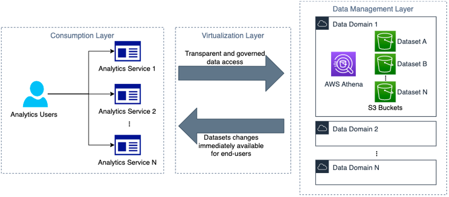
Jonatan Selsing is former research scientist with a PhD in astrophysics that has turned to the cloud. He is currently the Lead Cloud Engineer at Novo Nordisk, where he enables data and analytics workloads at scale. With an emphasis on reducing the total cost of ownership of cloud-based workloads, while giving full benefit of the advantages of cloud, he designs, builds, and maintains solutions that enable research for future medicines.

Hassen Riahi is a Sr. Data Architect at AWS Professional Services. He holds a PhD in Mathematics & Computer Science on large-scale data management. He works with AWS customers on building data-driven solutions.

Alessandro Fior is a Sr. Data Architect at AWS Professional Services. He is passionate about designing and building modern and scalable data platforms that accelerate companies to extract value from their data.

Moses Arthur comes from a mathematics and computational research background and holds a PhD in Computational Intelligence specialized in Graph Mining. He is currently a Cloud Product Engineer at Novo Nordisk, building GxP-compliant enterprise data lakes and analytics platforms for Novo Nordisk global factories producing digitalized medical products.

Anwar RizalAnwar Rizal is a Senior Machine Learning consultant based in Paris. He works with AWS customers to develop data and AI solutions to sustainably grow their business.

Kumari RamarKumari Ramar is an Agile certified and PMP certified Senior Engagement Manager at AWS Professional Services. She delivers data and AI/ML solutions that speed up cross-system analytics and machine learning models, which enable enterprises to make data-driven decisions and drive new innovations.

Top strategies for high volume tracing with Amazon OpenSearch Ingestion

Post Syndicated from Muthu Pitchaimani original https://aws.amazon.com/blogs/big-data/top-strategies-for-high-volume-tracing-with-amazon-opensearch-ingestion/

Amazon OpenSearch Ingestion is a serverless, auto-scaled, managed data collector that receives, transforms, and delivers data to Amazon OpenSearch Service domains or Amazon OpenSearch Serverless collections. OpenSearch Ingestion is powered by Data Prepper, an open-source, streaming ETL (extract, transform, and load) solution that’s part of the OpenSearch project. When you use OpenSearch Ingestion, you don’t need to maintain self-managed data pipelines to ingest logs, traces, metrics, and other data with OpenSearch Service. Amazon OpenSearch Ingestion responds to changing volumes of data, automatically scaling your ingest pipeline.

Distributed tracing is the leading way to locate, alert on, and remediate problems with your application and infrastructure. Distributed tracing is part of a broader observability solution, often combined with metrics and log data. OpenSearch Service gives you a native toolset to store and analyze large volumes of log, metric, and trace data. However, moving these large volumes of data is non-trivial to set up, monitor, and maintain.

In this post, we outline steps to set up a trace pipeline and strategies to deal with high volume tracing with Amazon OpenSearch Ingestion.

Solution overview

There is now a new option on the OpenSearch Service console called Pipelines under Ingestion in the navigation pane. We use this feature to create a trace pipeline.

You can also use the AWS Command Line Interface (AWS CLI), AWS CloudFormation, or AWS APIs to create a trace pipeline.

Prerequisites

Refer to Security in OpenSearch Ingestion to set up the permissions you need to create a pipeline and write to a pipeline, and the permissions the pipeline needs to write to a sink.

Create a trace pipeline

To create a trace pipeline, complete the following steps:

  1. On the OpenSearch Service console, choose Pipelines under Ingestion in the navigation pane.
  2. Choose Create pipeline.

Amazon OpenSearch Ingestion, powered by Data Prepper, uses pipelines as a mechanism to move the data from a source to a sink, with optional processors to mutate, route, sample, and detect anomalies for the data in the pipe. For more information, refer to Data Prepper. When you use Data Prepper, you build a YAML configuration file. When you use OpenSearch Ingestion, you upload your YAML configuration to the service. If you’re using the OpenSearch Service console, you can use one of the configuration blueprints that we provide. For distributed tracing, you will use an otel_trace_source and an OpenSearch Service domain as the sink.

  1. On the Configuration blueprints menu, choose AWS-TraceAnalyticsPipeline.

Choosing this blueprint will create a sample pipeline with otel_trace_source, an OpenSearch sink, along with span-pipeline and service-map-pipeline.

  1. Enter a name for this pipeline along with a minimum (1) and maximum (96) capacity value for Ingestion-OCUs.

Amazon OpenSearch Ingestion will scale automatically between these values to suit the volume of data you are ingesting.

  1. Edit the configuration’s hosts, aws.sts_role_arn, and region fields of the OpenSearch Service sink.
  2. Follow rest of the steps to complete the trace pipeline creation.

Sample trace pipeline

The following code shows the components of a sample trace pipeline:

version: "2"
entry-pipeline: 
  source:
    otel_trace_source:
      path: "/${pipelineName}/v1/traces"
  processor:
    - trace_peer_forwarder:
  sink:
    - pipeline:
        name: "span-pipeline"
    - pipeline:
        name: "service-map-pipeline"
span-pipeline:
  source:
    pipeline:
      name: "entry-pipeline"
  processor:
    - otel_trace_raw:
  sink:
    - opensearch:
        hosts: [ "https://search-mydomain-1a2a3a4a5a6a7a8a9a0a9a8a7a.us-east-1.es.amazonaws.com" ]
        aws:
          sts_role_arn: "arn:aws:iam::123456789012:role/Example-Role"
          region: "us-east-1"
        index_type: "trace-analytics-raw"
service-map-pipeline:
  source:
    pipeline:
      name: "entry-pipeline"
  processor:
    - service_map_stateful:
  sink:
    - opensearch:
        hosts: [ "https://search-mydomain-1a2a3a4a5a6a7a8a9a0a9a8a7a.us-east-1.es.amazonaws.com" ]
        aws:
          sts_role_arn: "arn:aws:iam::123456789012:role/Example-Role"
          region: "us-east-1"
        index_type: "trace-analytics-service-map"

The sample trace pipeline has three sub-pipelines in its configuration. These are entry-pipeline, span-pipeline, and service-map-pipeline. The following diagram illustrates the workflow.

entry-pipeline specifies the source of data as otel_trace_source, which creates an HTTP listener for receiving OpenTelemetry traces at the ingestion URL for the pipeline. You use a trace_peer_forwarder processor to eliminate duplicate HTTP requests and forward the data to the span-pipeline and service-map pipelines. span-pipeline gets the raw trace data from entry-pipeline and uses the otel_trace_raw processor to complete trace group-related fields for the incoming span records. You use the service_map_stateful processor to have Data Prepper create the distributed service map for visualization in OpenSearch Dashboards. After the sample trace pipeline is created, it’s ready to receive OpenTelemetry traces at its ingestion URL!

Reduce your storage footprint and optimize for cost

The volume of traces collected from instrumenting a modern production enterprise application can reach tens or hundreds of terabytes very quickly, especially when you store every trace from every request. The problem of managing the storage footprint becomes important. In this section, we discuss strategies for reducing your storage footprint and optimizing for cost.

Use storage tiering

OpenSearch Service has three storage tiers: hot, UltraWarm, and cold. You use the hot tier to store frequently accessed data for quick reading and writing, the UltraWarm tier for infrequently used, read-only data backed by Amazon Simple Storage Service (Amazon S3) for lower cost, and the cold tier to maintain re-attachable data at near-Amazon S3 cost. By adjusting relative retention periods between these tiers, you can store a high volume of traces. For example, instead of storing 1 weeks’ worth of traces in the hot tier, you can store 2 days of traces in the hot tier and 15 days in the UltraWarm tier.

Extract metrics without storing traces

You can also use Data Prepper’s aggregation process to extract metrics in the pipeline to avoid delivering all of your data to OpenSearch Service. For example, you may want to analyze request, error, and duration (RED) metrics of your traces to know the current state of your services. OpenSearch Ingestion can calculate these metrics in the pipeline, aggregating them and storing them in separate indexes for analysis, reducing the ingestion and storage footprint of your traces. The following pipeline configuration snippet shows how to use the aggregate processor to calculate a histogram of the duration metric:

...
  processor:
    - aggregate:
        identification_keys: ["serviceName", "traceId"]
        action:
          histogram:
            key: "durationInNanos"
            record_minmax: true
            units: "nanoseconds"
            buckets: [1000000000, 1500000000, 2000000000]
        group_duration: "20s"
   sink:
    - opensearch:
        hosts: ...
        aws_sts_role_arn: ...
        aws_region: ...
        aws_sigv4: true
        index: "red_metrics_from_traces"
  ...

Use sampling

When your application is running without issues, the proportion of error traces is just a small percentage of your overall trace volume. Storing all of the traces for successful requests increases the cost substantially, while offering low value. To reduce cost, you can sample your trace data, reducing the number of traces you store in OpenSearch Service. There are generally two techniques for sampling:

  • Head sampling – When you do head sampling, you ask OpenSearch Ingestion to make a sampling decision without looking at the whole trace. Head sampling is easy to configure and is efficient, but has a downside of possibly missing important traces.
  • Tail sampling – Tail sampling is where you analyze the entirety of the trace and then decide whether to sample the trace or not. This accurately captures all the needed traces at the cost of complexity in configuring and implementing.

The following configuration snippet shows an example of the percent_sampler, from the aggregate processor. In this example, you send only 25% of your traces to OpenSearch Service, based on head sampling:

  ...
  processor:
    - aggregate:
        identification_keys: ["serviceName"]
        action:
          percent_sampler:
            percent: 25
        group_duration: "30s"
  sink:
    - opensearch:
        hosts: ...
        aws_sts_role_arn: ...
        aws_region: ...
        aws_sigv4: true
        index: "sampled-traces"
  ...

Use conditional routing with sampling

Head sampling using the percentage_sampler is simple and straightforward, but is a blunt tool. A better way to sample would be to gather, for example, 10% of successful responses, and 100% of failed responses or 100% high duration traces. To solve this, use conditional routing. Routes define conditions that can be used within processors and sinks to direct the data flowing through different parts of pipeline. For example, the following configuration snippet routes traces whose status code indicates a failure to the error_trace pipeline. You forward 100% of the data in that pipe. You route traces whose duration metric is more than 1 second to the high_latency pipeline where you sample them at 80%. Other normal traces are only sampled at 20%.

  processor:
    - otel_trace_raw:
  route:
    - error_traces: "/traceGroupFields/statusCode == 2"
    - high_latency_traces: '/durationInNanos >= 1000000000'
    - normal_traces: '/traceGroupFields/statusCode!= 2 and /durationInNanos < 1000000000'
  sink:
    - pipeline:
        name: "trace-error-pipeline"
        routes:
          - error_traces
    - pipeline: 
        name: "trace-high-latency-metrics-pipeline"
        routes: 
          - high_latency_traces
    - pipeline: 
        name: "trace-normal-pipeline"
        routes: 
          - normal_traces
  ...

Conclusion

In this post, you learned how to configure an OpenSearch Ingestion pipeline and several strategies to keep in mind that help minimize cost while supporting a large-scale production system for distributed tracing. As next step, refer to the Amazon OpenSearch Developer Guide to explore logs and metric pipelines that you can use to build a scalable observability solution for your enterprise applications.


About the author

Muthu Pitchaimani is a Search Specialist with Amazon OpenSearch Service. He builds large-scale search applications and solutions. Muthu is interested in the topics of networking and security, and is based out of Austin, Texas.

Perform upserts in a data lake using Amazon Athena and Apache Iceberg

Post Syndicated from Ranjit Rajan original https://aws.amazon.com/blogs/big-data/perform-upserts-in-a-data-lake-using-amazon-athena-and-apache-iceberg/

Amazon Athena supports the MERGE command on Apache Iceberg tables, which allows you to perform inserts, updates, and deletes in your data lake at scale using familiar SQL statements that are compliant with ACID (Atomic, Consistent, Isolated, Durable). Apache Iceberg is an open table format for data lakes that manages large collections of files as tables. It supports modern analytical data lake operations such as create table as select (CTAS), upsert and merge, and time travel queries. Athena also supports the ability to create views and perform VACUUM (snapshot expiration) on Apache Iceberg tables to optimize storage and performance. With these features, you can now build data pipelines completely in standard SQL that are serverless, more simple to build, and able to operate at scale. This enables developers to:

  • Focus on writing business logic and not worry about setting up and managing the underlying infrastructure
  • Perform data transformations with Athena
  • Help comply with certain data deletion requirements
  • Apply change data capture (CDC) from sources databases

With data lakes, data pipelines are typically configured to write data into a raw zone, which is an Amazon Simple Storage Service (Amazon S3) bucket or folder that contains data as is from source systems. Data is accumulated in this zone, such that inserts, updates, or deletes on the sources database appear as records in new files as transactions occur on the source. Although the raw zone can be queried, any downstream processing or analytical queries typically need to deduplicate data to derive a current view of the source table. For example, if a single record is updated multiple times in the source database, these be need to be deduplicated and the most recent record selected.

Typically, data transformation processes are used to perform this operation, and a final consistent view is stored in an S3 bucket or folder. Data transformation processes can be complex requiring more coding, more testing and are also error prone. This was a challenge because data lakes are based on files and have been optimized for appending data. Previously, you had to overwrite the complete S3 object or folder, which was not only inefficient but also interrupted users who were querying the same data. With the evolution of frameworks such as Apache Iceberg, you can perform SQL-based upsert in-place in Amazon S3 using Athena, without blocking user queries and while still maintaining query performance.

In this post, we demonstrate how you can use Athena to apply CDC from a relational database to target tables in an S3 data lake.

Overview of solution

For this post, consider a mock sports ticketing application based on the following project. We use a single table in that database that contains sporting events information and ingest it into an S3 data lake on a continuous basis (initial load and ongoing changes). This data ingestion pipeline can be implemented using AWS Database Migration Service (AWS DMS) to extract both full and ongoing CDC extracts. With CDC, you can determine and track data that has changed and provide it as a stream of changes that a downstream application can consume. Most databases use a transaction log to record changes made to the database. AWS DMS reads the transaction log by using engine-specific API operations and captures the changes made to the database in a nonintrusive manner.

Specifically, to extract changed data including inserts, updates, and deletes from the database, you can configure AWS DMS with two replication tasks, as described in the following workshop. The first task performs an initial copy of the full data into an S3 folder. The second task is configured to replicate ongoing CDC into a separate folder in S3, which is further organized into date-based subfolders based on the source databases’ transaction commit date. With full and CDC data in separate S3 folders, it’s easier to maintain and operate data replication and downstream processing jobs. To enable this, you can apply the following extra connection attributes to the S3 endpoint in AWS DMS, (refer to S3Settings for other CSV and related settings):

  • TimestampColumnName – AWS DMS adds a column that you name with timestamp information for the commit of that row in the source database.
  • includeOpForFullLoad – AWS DMS adds a column named Op to every file to indicate if the record is an I (INSERT), U (UPDATE), or D (DELETE).
  • DatePartitionEnabled, DatePartitionSequence, DatePartitionDelimiter – These settings are used to configure AWS DMS to write changed data to date/time-based folders in the data lake. By partitioning folders, you can better manage S3 objects and optimize data lake queries for subsequent downstream processing.

We use the support in Athena for Apache Iceberg tables called MERGE INTO, which can express row-level updates. Apache Iceberg supports MERGE INTO by rewriting data files that contain rows that need to be updated. After the data is merged, we demonstrate how to use Athena to perform time travel on the sporting_event table, and use views to abstract and present different versions of the data to end-users. Finally, to simplify table maintenance, we demonstrate performing VACUUM on Apache Iceberg tables to delete older snapshots, which will optimize latency and cost of both read and write operations.

The following diagram illustrates the solution architecture.

The solution workflow consists of the following steps:

  • Data ingestion:
    • Steps 1 and 2 use AWS DMS, which connects to the source database to load initial data and ongoing changes (CDC) to Amazon S3 in CSV format. For this post, we have provided sample full and CDC datasets in CSV format that have been generated using AWS DMS.
    • Step 3 is comprised of the following actions:
      • Create an external table in Athena pointing to the source data ingested in Amazon S3.
      • Create an Apache Iceberg target table and load data from the source table.
      • Merge CDC data into the Apache Iceberg table using MERGE INTO.
  • Data access:
    • In Step 4, create a view on the Apache Iceberg table.
    • Use the view to query data using standard SQL.

Prerequisites

Before getting started, make sure you have the required permissions to perform the following in your AWS account:

Create tables on the raw data

First, create a database for this demo.

  1. Navigate to the Athena console and choose Query editor.
    If this is your first time using the Athena query editor, you need to configure and specify an S3 bucket to store the query results.
  2. Create a database with the following code:
    CREATE DATABASE raw_demo;

  3. Next, create a folder in an S3 bucket that you can use for this demo. Name this folder sporting_event_full.
  4. Upload LOAD00000001.csv into the folder.
  5. Switch to the raw_demo database and create a table to point to the raw input data:
    CREATE EXTERNAL TABLE raw_demo.sporting_event(
      op string,
      cdc_timestamp timestamp, 
      id bigint, 
      sport_type_name string, 
      home_team_id int, 
      away_team_id int, 
      location_id smallint, 
      start_date_time timestamp, 
      start_date date, 
      sold_out smallint)
    ROW FORMAT DELIMITED 
      FIELDS TERMINATED BY ',' 
    STORED AS INPUTFORMAT 'org.apache.hadoop.mapred.TextInputFormat' 
    OUTPUTFORMAT 'org.apache.hadoop.hive.ql.io.HiveIgnoreKeyTextOutputFormat'
    LOCATION 's3://<your bucket>/sporting_event_full/'
      ;

  6. Run the following query to review the data:
    SELECT * FROM raw_demo.sporting_event LIMIT 5;

  7. Next, create another folder in the same S3 bucket called sporting_event_cdc.
  8. Within this folder, create three subfolders in a time hierarchy folder structure such that the final S3 folder URI looks like s3://<your-bucket>/sporting_event_cdc/2022/09/22/.
  9. Upload 20220922-184314489.csv into this folder.This folder structure is similar to how AWS DMS stores CDC data when you enable date-based folder partitioning.
  10. Create a table to point to the CDC data. This table also includes a partition column because the source data in Amazon S3 is organized into date-based folders.
    CREATE EXTERNAL TABLE raw_demo.sporting_event_cdc(
    op string,
    cdc_timestamp timestamp,
    id bigint,
    sport_type_name string,
    home_team_id int,
    away_team_id int,
    location_id smallint,
    start_date_time timestamp,
    start_date date,
    sold_out smallint)
    PARTITIONED BY (partition_date string)
    ROW FORMAT DELIMITED
    FIELDS TERMINATED BY ','
    STORED AS INPUTFORMAT 'org.apache.hadoop.mapred.TextInputFormat'
    OUTPUTFORMAT 'org.apache.hadoop.hive.ql.io.HiveIgnoreKeyTextOutputFormat'
    LOCATION 's3://<your-bucket>/sporting_event_cdc/'
    ;

  11. Next, alter the table to add new partitions. Because the data is stored in non-Hive style format by AWS DMS, to query this data, add this partition manually or use an AWS Glue crawler. As data accumulates, continue to add new partitions to query this data.
    ALTER TABLE raw_demo.sporting_event_cdc ADD PARTITION (partition_date='2022-09-22') location 's3://<your-bucket>/sporting_event_cdc/2022/09/22/'

  12. Run the following query to review the CDC data:
    SELECT * FROM raw_demo.sporting_event_cdc;

There are two records with IDs 1 and 11 that are updates with op code U. The record with ID 21 has a delete (D) op code, and the record with ID 5 is an insert (I).

cdc data

Use CTAS to create the target Iceberg table in Parquet format

CTAS statements create new tables using standard SELECT queries. The resultant table is added to the AWS Glue Data Catalog and made available for querying.

  1. First, create another database to store the target table:
    CREATE DATABASE curated_demo;

  2. Next, switch to this database and run the CTAS statement to select data from the raw input table to create the target Iceberg table (replace the location with an appropriate S3 bucket in your account):
    CREATE TABLE curated_demo.sporting_event
    WITH (table_type='ICEBERG',
    location='s3://<your-bucket>/curated/sporting_event',
    format='PARQUET',
    is_external=false)
    AS SELECT
    id,
    sport_type_name,
    home_team_id,
    away_team_id,
    cast(location_id as int) as location_id,
    cast(start_date_time as timestamp(6)) as start_date_time,
    start_date,
    cast(sold_out as int) as sold_out
    FROM raw_demo.sporting_event
    ;

  3. Run the following query to review data in the Iceberg table:
    SELECT * FROM curated_demo.sporting_event LIMIT 5;

iceberg data

Use MERGE INTO to insert, update, and delete data into the Iceberg table

The MERGE INTO command updates the target table with data from the CDC table. The following statement uses a combination of primary keys and the Op column in the source data, which indicates if the source row is an insert, update, or delete. We use the id column as the primary key to join the target table to the source table, and we use the Op column to determine if a record needs to be deleted.

MERGE INTO curated_demo.sporting_event t
USING (SELECT op,
cdc_timestamp,
id,
sport_type_name,
home_team_id,
away_team_id,
location_id,
start_date_time,
start_date,
sold_out
FROM raw_demo.sporting_event_cdc
WHERE partition_date ='2022-09-22') s
ON t.id = s.id
WHEN MATCHED AND s.op = 'D' THEN DELETE
WHEN MATCHED THEN
UPDATE SET
sport_type_name = s.sport_type_name,
home_team_id = s.home_team_id,
location_id = s.location_id,
start_date_time = s.start_date_time,
start_date = s.start_date,
sold_out = s.sold_out
WHEN NOT MATCHED THEN
INSERT (id,
sport_type_name,
home_team_id,
away_team_id,
location_id,
start_date_time,
start_date)
VALUES
(s.id,
s.sport_type_name,
s.home_team_id,
s.away_team_id,
s.location_id,
s.start_date_time,
s.start_date)

Run the following query to verify data in the Iceberg table:

SELECT * FROM curated_demo.sporting_event WHERE id in (1, 5, 11, 21);

The record with ID 21 has been deleted, and the other records in the CDC dataset have been updated and inserted, as expected.

merge and delete

Create a view that contains the previous state

When you write to an Iceberg table, a new snapshot or version of a table is created each time.

A snapshot represents the state of a table at a point in time and is used to access the complete set of data files in the table. Time travel queries in Athena query Amazon S3 for historical data from a consistent snapshot as of a specified date and time or a specified snapshot ID. However, this requires knowledge of a table’s current snapshots. To abstract this information from users, you can create views on top of Iceberg tables:

CREATE VIEW curated_demo.v_sporting_event_previous_snapshot AS
SELECT id,
sport_type_name,
home_team_id,
away_team_id,
location_id,
cast(start_date_time as timestamp(3)) as start_date_time,
start_date,
sold_out
FROM curated_demo.sporting_event
FOR TIMESTAMP AS OF current_timestamp + interval '-5' minute;

Run the following query using this view to retrieve the snapshot of data before the CDC was applied:

SELECT * FROM curated_demo.v_sporting_event_previous_snapshot WHERE id = 21;

You can see the record with ID 21, which was deleted earlier.

view data

Compliance with privacy regulations may require that you permanently delete records in all snapshots. To accomplish this, you can set properties for snapshot retention in Athena when creating the table, or you can alter the table:

ALTER TABLE curated_demo.sporting_event SET TBLPROPERTIES (
'vacuum_min_snapshots_to_keep'='1',
'vacuum_max_snapshot_age_seconds'='1'
)

This instructs Athena to store only one version of the data and not maintain any transaction history. After a table has been updated with these properties, run the VACUUM command to remove the older snapshots and clean up storage:

VACUUM curated_demo.sporting_event;

Run the following query again:

SELECT * FROM curated_demo.v_sporting_event_previous_snapshot WHERE id = 21;

The record with ID 21 has been permanently deleted.

final validation

Considerations

As data accumulates in the CDC folder of your raw zone, older files can be archived to Amazon S3 Glacier. Subsequently, the MERGE INTO statement can also be run on a single source file if needed by using $path in the WHERE condition of the USING clause:

MERGE INTO curated_demo.sporting_event t
USING (SELECT op, cdc_timestamp,id,sport_type_name, home_team_id, away_team_id, location_id, start_date_time, start_date, sold_out FROM raw_demo.sporting_event_cdc WHERE partition_date='2022-09-22' AND regexp_like("$path", ‘/sporting_event_cdc/2022/09/22/20220922-184314489.csv')
………..

This results in Athena scanning all files in the partition’s folder before the filter is applied, but can be minimized by choosing fine-grained hourly partitions. With this approach, you can trigger the MERGE INTO to run on Athena as files arrive in your S3 bucket using Amazon S3 event notifications. This could enable near-real-time use cases where users need to query a consistent view of data in the data lake as soon it is created in source systems.

Clean up

To avoid incurring ongoing costs, complete the following steps to clean up your resources:

  1. Run the following SQL to drop the tables and views:
    DROP TABLE raw_demo.sporting_event;
    DROP TABLE raw_demo.sporting_event_cdc;
    DROP TABLE curated_demo.sporting_event;
    DROP VIEW curated_demo.v_sporting_event_previous_snapshot;

    Because Iceberg tables are considered managed tables in Athena, dropping an Iceberg table also removes all the data in the corresponding S3 folder.

  2. Run the following SQL to drop the databases:
    DROP DATABASE raw_demo;
    DROP DATABASE curated_demo;

  3. Delete the S3 folders and CSV files that you had uploaded.

Conclusion

This post showed you how to apply CDC to a target Iceberg table using CTAS and MERGE INTO statements in Athena. You can perform bulk load using a CTAS statement. When new data or changed data arrives, use the MERGE INTO statement to merge the CDC changes. To optimize storage and improve performance of queries, use the VACUUM command regularly.

As next steps, you can orchestrate these SQL statements using AWS Step Functions to implement end-to-end data pipelines for your data lake. For more information, refer to Build and orchestrate ETL pipelines using Amazon Athena and AWS Step Functions.


About the Authors

Ranjit Rajan is a Principal Data Lab Solutions Architect with AWS. Ranjit works with AWS customers to help them design and build data and analytics applications in the cloud.

Kannan Iyer is a Senior Data Lab Solutions Architect with AWS. Kannan works with AWS customers to help them design and build data and analytics applications in the cloud.

Alexandre Rezende is a Data Lab Solutions Architect with AWS. Alexandre works with customers on their Business Intelligence, Data Warehouse, and Data Lake use cases, design architectures to solve their business problems, and helps them build MVPs to accelerate their path to production.

How the BMW Group analyses semiconductor demand with AWS Glue

Post Syndicated from Göksel SARIKAYA original https://aws.amazon.com/blogs/big-data/how-the-bmw-group-analyses-semiconductor-demand-with-aws-glue/

This is a guest post co-written by Maik Leuthold and Nick Harmening from BMW Group.

The BMW Group is headquartered in Munich, Germany, where the company oversees 149,000 employees and manufactures cars and motorcycles in over 30 production sites across 15 countries. This multinational production strategy follows an even more international and extensive supplier network.

Like many automobile companies across the world, the BMW Group has been facing challenges in its supply chain due to the worldwide semiconductor shortage. Creating transparency about BMW Group’s current and future demand of semiconductors is one key strategic aspect to resolve shortages together with suppliers and semiconductor manufacturers. The manufacturers need to know BMW Group’s exact current and future semiconductor volume information, which will effectively help steer the available worldwide supply.

The main requirement is to have an automated, transparent, and long-term semiconductor demand forecast. Additionally, this forecasting system needs to provide data enrichment steps including byproducts, serve as the master data around the semiconductor management, and enable further use cases at the BMW Group.

To enable this use case, we used the BMW Group’s cloud-native data platform called the Cloud Data Hub. In 2019, the BMW Group decided to re-architect and move its on-premises data lake to the AWS Cloud to enable data-driven innovation while scaling with the dynamic needs of the organization. The Cloud Data Hub processes and combines anonymized data from vehicle sensors and other sources across the enterprise to make it easily accessible for internal teams creating customer-facing and internal applications. To learn more about the Cloud Data Hub, refer to BMW Group Uses AWS-Based Data Lake to Unlock the Power of Data.

In this post, we share how the BMW Group analyzes semiconductor demand using AWS Glue.

Logic and systems behind the demand forecast

The first step towards the demand forecast is the identification of semiconductor-relevant components of a vehicle type. Each component is described by a unique part number, which serves as a key in all systems to identify this component. A component can be a headlight or a steering wheel, for example.

For historic reasons, the required data for this aggregation step is siloed and represented differently in diverse systems. Because each source system and data type have its own schema and format, it’s particularly difficult to perform analytics based on this data. Some source systems are already available in the Cloud Data Hub (for example, part master data), therefore it’s straightforward to consume from our AWS account. To access the remaining data sources, we need to build specific ingest jobs that read data from the respective system.

The following diagram illustrates the approach.

The data enrichment starts with an Oracle Database (Software Parts) that contains part numbers that are related to software. This can be the control unit of a headlight or a camera system for automated driving. Because semiconductors are the basis for running software, this database builds the foundation of our data processing.

In the next step, we use REST APIs (Part Relations) to enrich the data with further attributes. This includes how parts are related (for example, a specific control unit that will be installed into a headlight) and over which timespan a part number will be built into a vehicle. The knowledge about the part relations is essential to understand how a specific semiconductor, in this case the control unit, is relevant for a more general part, the headlight. The temporal information about the use of part numbers allows us to filter out outdated part numbers, which will not be used in the future and therefore have no relevance in the forecast.

The data (Part Master Data) can directly be consumed from the Cloud Data Hub. This database includes attributes about the status and material types of a part number. This information is required to filter out part numbers that we gathered in the previous steps but have no relevance for semiconductors. With the information that was gathered from the APIs, this data is also queried to extract further part numbers that weren’t ingested in the previous steps.

After data enrichment and filtering, a third-party system reads the filtered part data and enriches the semiconductor information. Subsequently, it adds the volume information of the components. Finally, it provides the overall semiconductor demand forecast centrally to the Cloud Data Hub.

Applied services

Our solution uses the serverless services AWS Glue and Amazon Simple Storage Service (Amazon S3) to run ETL (extract, transform, and load) workflows without managing an infrastructure. It also reduces the costs by paying only for the time jobs are running. The serverless approach fits our workflow’s schedule very well because we run the workload only once a week.

Because we’re using diverse data source systems as well as complex processing and aggregation, it’s important to decouple ETL jobs. This allows us to process each data source independently. We also split the data transformation into several modules (Data Aggregation, Data Filtering, and Data Preparation) to make the system more transparent and easier to maintain. This approach also helps in case of extending or modifying existing jobs.

Although each module is specific to a data source or a particular data transformation, we utilize reusable blocks inside of every job. This allows us to unify each type of operation and simplifies the procedure of adding new data sources and transformation steps in the future.

In our setup, we follow the security best practice of the least privilege principle, to ensure the information is protected from accidental or unnecessary access. Therefore, each module has AWS Identity and Access Management (IAM) roles with only the necessary permissions, namely access to only data sources and buckets the job deals with. For more information regarding security best practices, refer to Security best practices in IAM.

Solution overview

The following diagram shows the overall workflow where several AWS Glue jobs are interacting with each other sequentially.

As we mentioned earlier, we used the Cloud Data Hub, Oracle DB, and other data sources that we communicate with via the REST API. The first step of the solution is the Data Source Ingest module, which ingests the data from different data sources. For that purpose, AWS Glue jobs read information from different data sources and writes into the S3 source buckets. Ingested data is stored in the encrypted buckets, and keys are managed by AWS Key Management Service (AWS KMS).

After the Data Source Ingest step, intermediate jobs aggregate and enrich the tables with other data sources like components version and categories, model manufacture dates, and so on. Then they write them into the intermediate buckets in the Data Aggregation module, creating comprehensive and abundant data representation. Additionally, according to the business logic workflow, the Data Filtering and Data Preparation modules create the final master data table with only actual and production-relevant information.

The AWS Glue workflow manages all these ingestion jobs and filtering jobs end to end. An AWS Glue workflow schedule is configured weekly to run the workflow on Wednesdays. While the workflow is running, each job writes execution logs (info or error) into Amazon Simple Notification Service (Amazon SNS) and Amazon CloudWatch for monitoring purposes. Amazon SNS forwards the execution results to the monitoring tools, such as Mail, Teams, or Slack channels. In case of any error in the jobs, Amazon SNS also alerts the listeners about the job execution result to take action.

As the last step of the solution, the third-party system reads the master table from the prepared data bucket via Amazon Athena. After further data engineering steps like semiconductor information enrichment and volume information integration, the final master data asset is written into the Cloud Data Hub. With the data now provided in the Cloud Data Hub, other use cases can use this semiconductor master data without building several interfaces to different source systems.

Business outcome

The project results provide the BMW Group a substantial transparency about their semiconductor demand for their entire vehicle portfolio in the present and in the future. The creation of a database with that magnitude enables the BMW Group to establish even further use cases to the benefit of more supply chain transparency and clearer and deeper exchange with first-tier suppliers and semiconductor manufacturers. It helps not only to resolve the current demanding market situation, but also to be more resilient in the future. Therefore, it’s one major step to a digital, transparent supply chain.

Conclusion

This post describes how to analyze semiconductor demand from many data sources with big data jobs in an AWS Glue workflow. A serverless architecture with minimal diversity of services makes the code base and architecture simple to understand and maintain. To learn more about how to use AWS Glue workflows and jobs for serverless orchestration, visit the AWS Glue service page.


About the authors

Maik Leuthold is a Project Lead at the BMW Group for advanced analytics in the business field of supply chain and procurement, and leads the digitalization strategy for the semiconductor management.

Nick Harmening is an IT Project Lead at the BMW Group and an AWS certified Solutions Architect. He builds and operates cloud-native applications with a focus on data engineering and machine learning.

Göksel Sarikaya is a Senior Cloud Application Architect at AWS Professional Services. He enables customers to design scalable, cost-effective, and competitive applications through the innovative production of the AWS platform. He helps them to accelerate customer and partner business outcomes during their digital transformation journey.

Alexander Tselikov is a Data Architect at AWS Professional Services who is passionate about helping customers to build scalable data, analytics and ML solutions to enable timely insights and make critical business decisions.

Rahul Shaurya is a Senior Big Data Architect at Amazon Web Services. He helps and works closely with customers building data platforms and analytical applications on AWS. Outside of work, Rahul loves taking long walks with his dog Barney.