Post Syndicated from Danilo Poccia original https://aws.amazon.com/blogs/aws/amazon-nova-multimodal-embeddings-now-available-in-amazon-bedrock/
Today, we’re introducing Amazon Nova Multimodal Embeddings, a state-of-the-art multimodal embedding model for agentic retrieval-augmented generation (RAG) and semantic search applications, available in Amazon Bedrock. It is the first unified embedding model that supports text, documents, images, video, and audio through a single model to enable crossmodal retrieval with leading accuracy.
Embedding models convert textual, visual, and audio inputs into numerical representations called embeddings. These embeddings capture the meaning of the input in a way that AI systems can compare, search, and analyze, powering use cases such as semantic search and RAG.
Organizations are increasingly seeking solutions to unlock insights from the growing volume of unstructured data that is spread across text, image, document, video, and audio content. For example, an organization might have product images, brochures that contain infographics and text, and user-uploaded video clips. Embedding models are able to unlock value from unstructured data, however traditional models are typically specialized to handle one content type. This limitation drives customers to either build complex crossmodal embedding solutions or restrict themselves to use cases focused on a single content type. The problem also applies to mixed-modality content types such as documents with interleaved text and images or video with visual, audio, and textual elements where existing models struggle to capture crossmodal relationships effectively.
Nova Multimodal Embeddings supports a unified semantic space for text, documents, images, video, and audio for use cases such as crossmodal search across mixed-modality content, searching with a reference image, and retrieving visual documents.
Evaluating Amazon Nova Multimodal Embeddings performance
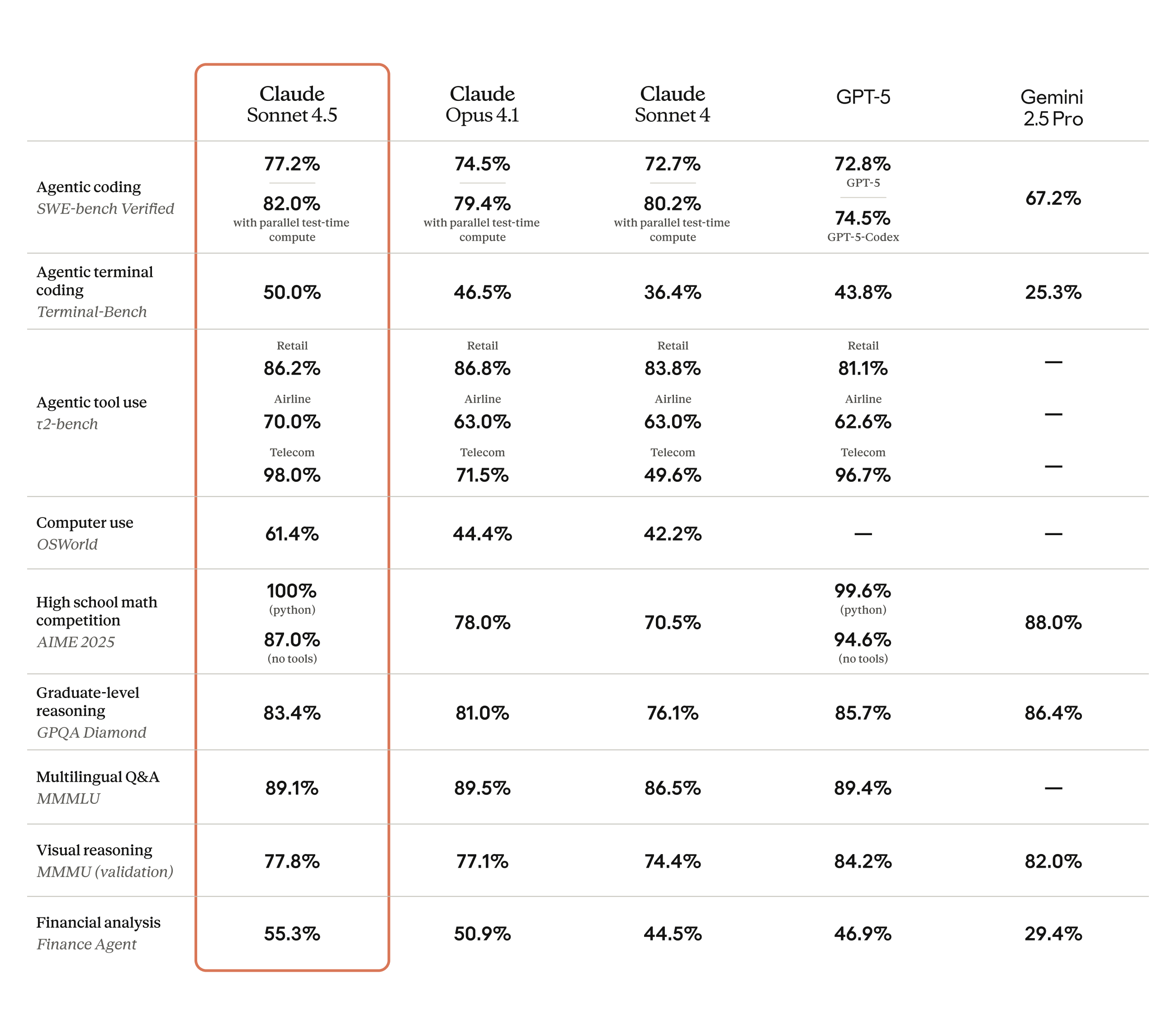
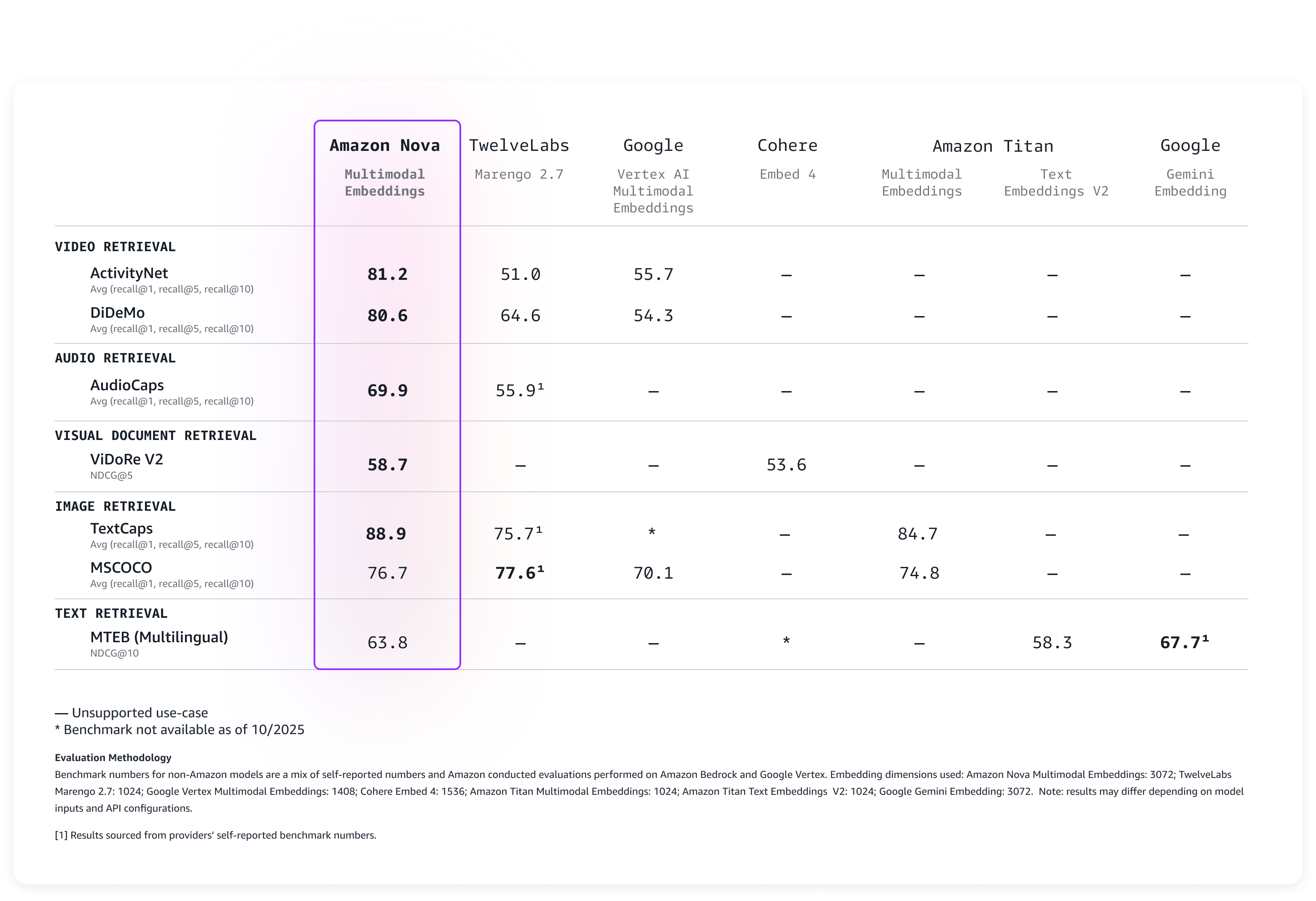
We evaluated the model on a broad range of benchmarks, and it delivers leading accuracy out-of-the-box as described in the following table.

Nova Multimodal Embeddings supports a context length of up to 8K tokens, text in up to 200 languages, and accepts inputs via synchronous and asynchronous APIs. Additionally, it supports segmentation (also known as “chunking”) to partition long-form text, video, or audio content into manageable segments, generating embeddings for each portion. Lastly, the model offers four output embedding dimensions, trained using Matryoshka Representation Learning (MRL) that enables low-latency end-to-end retrieval with minimal accuracy changes.
Let’s see how the new model can be used in practice.
Using Amazon Nova Multimodal Embeddings
Getting started with Nova Multimodal Embeddings follows the same pattern as other models in Amazon Bedrock. The model accepts text, documents, images, video, or audio as input and returns numerical embeddings that you can use for semantic search, similarity comparison, or RAG.
Here’s a practical example using the AWS SDK for Python (Boto3) that shows how to create embeddings from different content types and store them for later retrieval. For simplicity, I’ll use Amazon S3 Vectors, a cost-optimized storage with native support for storing and querying vectors at any scale, to store and search the embeddings.
Let’s start with the fundamentals: converting text into embeddings. This example shows how to transform a simple text description into a numerical representation that captures its semantic meaning. These embeddings can later be compared with embeddings from documents, images, videos, or audio to find related content.
To make the code easy to follow, I’ll show a section of the script at a time. The full script is included at the end of this walkthrough.
import json
import base64
import time
import boto3
MODEL_ID = "amazon.nova-2-multimodal-embeddings-v1:0"
EMBEDDING_DIMENSION = 3072
# Initialize Amazon Bedrock Runtime client
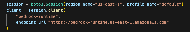
bedrock_runtime = boto3.client("bedrock-runtime", region_name="us-east-1")
print(f"Generating text embedding with {MODEL_ID} ...")
# Text to embed
text = "Amazon Nova is a multimodal foundation model"
# Create embedding
request_body = {
"taskType": "SINGLE_EMBEDDING",
"singleEmbeddingParams": {
"embeddingPurpose": "GENERIC_INDEX",
"embeddingDimension": EMBEDDING_DIMENSION,
"text": {"truncationMode": "END", "value": text},
},
}
response = bedrock_runtime.invoke_model(
body=json.dumps(request_body),
modelId=MODEL_ID,
contentType="application/json",
)
# Extract embedding
response_body = json.loads(response["body"].read())
embedding = response_body["embeddings"][0]["embedding"]
print(f"Generated embedding with {len(embedding)} dimensions")
Now we’ll process visual content using the same embedding space using a photo.jpg file in the same folder as the script. This demonstrates the power of multimodality: Nova Multimodal Embeddings is able to capture both textual and visual context into a single embedding that provides enhanced understanding of the document.
Nova Multimodal Embeddings can generate embeddings that are optimized for how they are being used. When indexing for a search or retrieval use case, embeddingPurpose can be set to GENERIC_INDEX. For the query step, embeddingPurpose can be set depending on the type of item to be retrieved. For example, when retrieving documents, embeddingPurpose can be set to DOCUMENT_RETRIEVAL.
# Read and encode image
print(f"Generating image embedding with {MODEL_ID} ...")

with open("photo.jpg", "rb") as f:
    image_bytes = base64.b64encode(f.read()).decode("utf-8")

# Create embedding
request_body = {
    "taskType": "SINGLE_EMBEDDING",
    "singleEmbeddingParams": {
        "embeddingPurpose": "GENERIC_INDEX",
        "embeddingDimension": EMBEDDING_DIMENSION,
        "image": {
            "format": "jpeg",
            "source": {"bytes": image_bytes}
        },
    },
}

response = bedrock_runtime.invoke_model(
    body=json.dumps(request_body),
    modelId=MODEL_ID,
    contentType="application/json",
)

# Extract embedding
response_body = json.loads(response["body"].read())
embedding = response_body["embeddings"][0]["embedding"]

print(f"Generated embedding with {len(embedding)} dimensions")
To process video content, I use the asynchronous API. That’s a requirement for videos that are larger than 25MB when encoded as Base64. First, I upload a local video to an S3 bucket in the same AWS Region.
aws s3 cp presentation.mp4 s3://my-video-bucket/videos/
This example shows how to extract embeddings from both visual and audio components of a video file. The segmentation feature breaks longer videos into manageable chunks, making it practical to search through hours of content efficiently.
# Initialize Amazon S3 client
s3 = boto3.client("s3", region_name="us-east-1")

print(f"Generating video embedding with {MODEL_ID} ...")

# Amazon S3 URIs
S3_VIDEO_URI = "s3://my-video-bucket/videos/presentation.mp4"
S3_EMBEDDING_DESTINATION_URI = "s3://my-embedding-destination-bucket/embeddings-output/"

# Create async embedding job for video with audio
model_input = {
    "taskType": "SEGMENTED_EMBEDDING",
    "segmentedEmbeddingParams": {
        "embeddingPurpose": "GENERIC_INDEX",
        "embeddingDimension": EMBEDDING_DIMENSION,
        "video": {
            "format": "mp4",
            "embeddingMode": "AUDIO_VIDEO_COMBINED",
            "source": {
                "s3Location": {"uri": S3_VIDEO_URI}
            },
            "segmentationConfig": {
                "durationSeconds": 15  # Segment into 15-second chunks
            },
        },
    },
}

response = bedrock_runtime.start_async_invoke(
    modelId=MODEL_ID,
    modelInput=model_input,
    outputDataConfig={
        "s3OutputDataConfig": {
            "s3Uri": S3_EMBEDDING_DESTINATION_URI
        }
    },
)

invocation_arn = response["invocationArn"]
print(f"Async job started: {invocation_arn}")

# Poll until job completes
print("\nPolling for job completion...")
while True:
    job = bedrock_runtime.get_async_invoke(invocationArn=invocation_arn)
    status = job["status"]
    print(f"Status: {status}")

    if status != "InProgress":
        break
    time.sleep(15)

# Check if job completed successfully
if status == "Completed":
    output_s3_uri = job["outputDataConfig"]["s3OutputDataConfig"]["s3Uri"]
    print(f"\nSuccess! Embeddings at: {output_s3_uri}")

    # Parse S3 URI to get bucket and prefix
    s3_uri_parts = output_s3_uri[5:].split("/", 1)  # Remove "s3://" prefix
    bucket = s3_uri_parts[0]
    prefix = s3_uri_parts[1] if len(s3_uri_parts) > 1 else ""

    # AUDIO_VIDEO_COMBINED mode outputs to embedding-audio-video.jsonl
    # The output_s3_uri already includes the job ID, so just append the filename
    embeddings_key = f"{prefix}/embedding-audio-video.jsonl".lstrip("/")

    print(f"Reading embeddings from: s3://{bucket}/{embeddings_key}")

    # Read and parse JSONL file
    response = s3.get_object(Bucket=bucket, Key=embeddings_key)
    content = response['Body'].read().decode('utf-8')

    embeddings = []
    for line in content.strip().split('\n'):
        if line:
            embeddings.append(json.loads(line))

    print(f"\nFound {len(embeddings)} video segments:")
    for i, segment in enumerate(embeddings):
        print(f"  Segment {i}: {segment.get('startTime', 0):.1f}s - {segment.get('endTime', 0):.1f}s")
        print(f"    Embedding dimension: {len(segment.get('embedding', []))}")
else:
    print(f"\nJob failed: {job.get('failureMessage', 'Unknown error')}")
With our embeddings generated, we need a place to store and search them efficiently. This example demonstrates setting up a vector store using Amazon S3 Vectors, which provides the infrastructure needed for similarity search at scale. Think of this as creating a searchable index where semantically similar content naturally clusters together. When adding an embedding to the index, I use the metadata to specify the original format and the content being indexed.
# Initialize Amazon S3 Vectors client
s3vectors = boto3.client("s3vectors", region_name="us-east-1")

# Configuration
VECTOR_BUCKET = "my-vector-store"
INDEX_NAME = "embeddings"

# Create vector bucket and index (if they don't exist)
try:
    s3vectors.get_vector_bucket(vectorBucketName=VECTOR_BUCKET)
    print(f"Vector bucket {VECTOR_BUCKET} already exists")
except s3vectors.exceptions.NotFoundException:
    s3vectors.create_vector_bucket(vectorBucketName=VECTOR_BUCKET)
    print(f"Created vector bucket: {VECTOR_BUCKET}")

try:
    s3vectors.get_index(vectorBucketName=VECTOR_BUCKET, indexName=INDEX_NAME)
    print(f"Vector index {INDEX_NAME} already exists")
except s3vectors.exceptions.NotFoundException:
    s3vectors.create_index(
        vectorBucketName=VECTOR_BUCKET,
        indexName=INDEX_NAME,
        dimension=EMBEDDING_DIMENSION,
        dataType="float32",
        distanceMetric="cosine"
    )
    print(f"Created index: {INDEX_NAME}")

texts = [
    "Machine learning on AWS",
    "Amazon Bedrock provides foundation models",
    "S3 Vectors enables semantic search"
]

print(f"\nGenerating embeddings for {len(texts)} texts...")

# Generate embeddings using Amazon Nova for each text
vectors = []
for text in texts:
    response = bedrock_runtime.invoke_model(
        body=json.dumps({
            "taskType": "SINGLE_EMBEDDING",
            "singleEmbeddingParams": {
                "embeddingDimension": EMBEDDING_DIMENSION,
                "text": {"truncationMode": "END", "value": text}
            }
        }),
        modelId=MODEL_ID,
        accept="application/json",
        contentType="application/json"
    )

    response_body = json.loads(response["body"].read())
    embedding = response_body["embeddings"][0]["embedding"]

    vectors.append({
        "key": f"text:{text[:50]}",  # Unique identifier
        "data": {"float32": embedding},
        "metadata": {"type": "text", "content": text}
    })
    print(f"  ✓ Generated embedding for: {text}")

# Add all vectors to store in a single call
s3vectors.put_vectors(
    vectorBucketName=VECTOR_BUCKET,
    indexName=INDEX_NAME,
    vectors=vectors
)

print(f"\nSuccessfully added {len(vectors)} vectors to the store in one put_vectors call!")
This final example demonstrates the capability of searching across different content types with a single query, finding the most similar content regardless of whether it originated from text, images, videos, or audio. The distance scores help you understand how closely related the results are to your original query.
# Text to query
query_text = "foundation models"

print(f"\nGenerating embeddings for query '{query_text}' ...")

# Generate embeddings
response = bedrock_runtime.invoke_model(
    body=json.dumps({
        "taskType": "SINGLE_EMBEDDING",
        "singleEmbeddingParams": {
            "embeddingPurpose": "GENERIC_RETRIEVAL",
            "embeddingDimension": EMBEDDING_DIMENSION,
            "text": {"truncationMode": "END", "value": query_text}
        }
    }),
    modelId=MODEL_ID,
    accept="application/json",
    contentType="application/json"
)

response_body = json.loads(response["body"].read())
query_embedding = response_body["embeddings"][0]["embedding"]

print(f"Searching for similar embeddings...\n")

# Search for top 5 most similar vectors
response = s3vectors.query_vectors(
    vectorBucketName=VECTOR_BUCKET,
    indexName=INDEX_NAME,
    queryVector={"float32": query_embedding},
    topK=5,
    returnDistance=True,
    returnMetadata=True
)

# Display results
print(f"Found {len(response['vectors'])} results:\n")
for i, result in enumerate(response["vectors"], 1):
    print(f"{i}. {result['key']}")
    print(f"   Distance: {result['distance']:.4f}")
    if result.get("metadata"):
        print(f"   Metadata: {result['metadata']}")
    print()
Crossmodal search is one of the key advantages of multimodal embeddings. With crossmodal search, you can query with text and find relevant images. You can also search for videos using text descriptions, find audio clips that match certain topics, or discover documents based on their visual and textual content. For your reference, the full script with all previous examples merged together is here:
import json
import base64
import time
import boto3

MODEL_ID = "amazon.nova-2-multimodal-embeddings-v1:0"
EMBEDDING_DIMENSION = 3072

# Initialize Amazon Bedrock Runtime client
bedrock_runtime = boto3.client("bedrock-runtime", region_name="us-east-1")

print(f"Generating text embedding with {MODEL_ID} ...")

# Text to embed
text = "Amazon Nova is a multimodal foundation model"

# Create embedding
request_body = {
    "taskType": "SINGLE_EMBEDDING",
    "singleEmbeddingParams": {
        "embeddingPurpose": "GENERIC_INDEX",
        "embeddingDimension": EMBEDDING_DIMENSION,
        "text": {"truncationMode": "END", "value": text},
    },
}

response = bedrock_runtime.invoke_model(
    body=json.dumps(request_body),
    modelId=MODEL_ID,
    contentType="application/json",
)

# Extract embedding
response_body = json.loads(response["body"].read())
embedding = response_body["embeddings"][0]["embedding"]

print(f"Generated embedding with {len(embedding)} dimensions")
# Read and encode image
print(f"Generating image embedding with {MODEL_ID} ...")

with open("photo.jpg", "rb") as f:
    image_bytes = base64.b64encode(f.read()).decode("utf-8")

# Create embedding
request_body = {
    "taskType": "SINGLE_EMBEDDING",
    "singleEmbeddingParams": {
        "embeddingPurpose": "GENERIC_INDEX",
        "embeddingDimension": EMBEDDING_DIMENSION,
        "image": {
            "format": "jpeg",
            "source": {"bytes": image_bytes}
        },
    },
}

response = bedrock_runtime.invoke_model(
    body=json.dumps(request_body),
    modelId=MODEL_ID,
    contentType="application/json",
)

# Extract embedding
response_body = json.loads(response["body"].read())
embedding = response_body["embeddings"][0]["embedding"]

print(f"Generated embedding with {len(embedding)} dimensions")
# Initialize Amazon S3 client
s3 = boto3.client("s3", region_name="us-east-1")

print(f"Generating video embedding with {MODEL_ID} ...")

# Amazon S3 URIs
S3_VIDEO_URI = "s3://my-video-bucket/videos/presentation.mp4"

# Amazon S3 output bucket and location
S3_EMBEDDING_DESTINATION_URI = "s3://my-video-bucket/embeddings-output/"

# Create async embedding job for video with audio
model_input = {
    "taskType": "SEGMENTED_EMBEDDING",
    "segmentedEmbeddingParams": {
        "embeddingPurpose": "GENERIC_INDEX",
        "embeddingDimension": EMBEDDING_DIMENSION,
        "video": {
            "format": "mp4",
            "embeddingMode": "AUDIO_VIDEO_COMBINED",
            "source": {
                "s3Location": {"uri": S3_VIDEO_URI}
            },
            "segmentationConfig": {
                "durationSeconds": 15  # Segment into 15-second chunks
            },
        },
    },
}

response = bedrock_runtime.start_async_invoke(
    modelId=MODEL_ID,
    modelInput=model_input,
    outputDataConfig={
        "s3OutputDataConfig": {
            "s3Uri": S3_EMBEDDING_DESTINATION_URI
        }
    },
)

invocation_arn = response["invocationArn"]
print(f"Async job started: {invocation_arn}")

# Poll until job completes
print("\nPolling for job completion...")
while True:
    job = bedrock_runtime.get_async_invoke(invocationArn=invocation_arn)
    status = job["status"]
    print(f"Status: {status}")

    if status != "InProgress":
        break
    time.sleep(15)

# Check if job completed successfully
if status == "Completed":
    output_s3_uri = job["outputDataConfig"]["s3OutputDataConfig"]["s3Uri"]
    print(f"\nSuccess! Embeddings at: {output_s3_uri}")

    # Parse S3 URI to get bucket and prefix
    s3_uri_parts = output_s3_uri[5:].split("/", 1)  # Remove "s3://" prefix
    bucket = s3_uri_parts[0]
    prefix = s3_uri_parts[1] if len(s3_uri_parts) > 1 else ""

    # AUDIO_VIDEO_COMBINED mode outputs to embedding-audio-video.jsonl
    # The output_s3_uri already includes the job ID, so just append the filename
    embeddings_key = f"{prefix}/embedding-audio-video.jsonl".lstrip("/")

    print(f"Reading embeddings from: s3://{bucket}/{embeddings_key}")

    # Read and parse JSONL file
    response = s3.get_object(Bucket=bucket, Key=embeddings_key)
    content = response['Body'].read().decode('utf-8')

    embeddings = []
    for line in content.strip().split('\n'):
        if line:
            embeddings.append(json.loads(line))

    print(f"\nFound {len(embeddings)} video segments:")
    for i, segment in enumerate(embeddings):
        print(f"  Segment {i}: {segment.get('startTime', 0):.1f}s - {segment.get('endTime', 0):.1f}s")
        print(f"    Embedding dimension: {len(segment.get('embedding', []))}")
else:
    print(f"\nJob failed: {job.get('failureMessage', 'Unknown error')}")
# Initialize Amazon S3 Vectors client
s3vectors = boto3.client("s3vectors", region_name="us-east-1")

# Configuration
VECTOR_BUCKET = "my-vector-store"
INDEX_NAME = "embeddings"

# Create vector bucket and index (if they don't exist)
try:
    s3vectors.get_vector_bucket(vectorBucketName=VECTOR_BUCKET)
    print(f"Vector bucket {VECTOR_BUCKET} already exists")
except s3vectors.exceptions.NotFoundException:
    s3vectors.create_vector_bucket(vectorBucketName=VECTOR_BUCKET)
    print(f"Created vector bucket: {VECTOR_BUCKET}")

try:
    s3vectors.get_index(vectorBucketName=VECTOR_BUCKET, indexName=INDEX_NAME)
    print(f"Vector index {INDEX_NAME} already exists")
except s3vectors.exceptions.NotFoundException:
    s3vectors.create_index(
        vectorBucketName=VECTOR_BUCKET,
        indexName=INDEX_NAME,
        dimension=EMBEDDING_DIMENSION,
        dataType="float32",
        distanceMetric="cosine"
    )
    print(f"Created index: {INDEX_NAME}")

texts = [
    "Machine learning on AWS",
    "Amazon Bedrock provides foundation models",
    "S3 Vectors enables semantic search"
]

print(f"\nGenerating embeddings for {len(texts)} texts...")

# Generate embeddings using Amazon Nova for each text
vectors = []
for text in texts:
    response = bedrock_runtime.invoke_model(
        body=json.dumps({
            "taskType": "SINGLE_EMBEDDING",
            "singleEmbeddingParams": {
                "embeddingPurpose": "GENERIC_INDEX",
                "embeddingDimension": EMBEDDING_DIMENSION,
                "text": {"truncationMode": "END", "value": text}
            }
        }),
        modelId=MODEL_ID,
        accept="application/json",
        contentType="application/json"
    )

    response_body = json.loads(response["body"].read())
    embedding = response_body["embeddings"][0]["embedding"]

    vectors.append({
        "key": f"text:{text[:50]}",  # Unique identifier
        "data": {"float32": embedding},
        "metadata": {"type": "text", "content": text}
    })
    print(f"  ✓ Generated embedding for: {text}")

# Add all vectors to store in a single call
s3vectors.put_vectors(
    vectorBucketName=VECTOR_BUCKET,
    indexName=INDEX_NAME,
    vectors=vectors
)

print(f"\nSuccessfully added {len(vectors)} vectors to the store in one put_vectors call!")
# Text to query
query_text = "foundation models"

print(f"\nGenerating embeddings for query '{query_text}' ...")

# Generate embeddings
response = bedrock_runtime.invoke_model(
    body=json.dumps({
        "taskType": "SINGLE_EMBEDDING",
        "singleEmbeddingParams": {
            "embeddingPurpose": "GENERIC_RETRIEVAL",
            "embeddingDimension": EMBEDDING_DIMENSION,
            "text": {"truncationMode": "END", "value": query_text}
        }
    }),
    modelId=MODEL_ID,
    accept="application/json",
    contentType="application/json"
)

response_body = json.loads(response["body"].read())
query_embedding = response_body["embeddings"][0]["embedding"]

print(f"Searching for similar embeddings...\n")

# Search for top 5 most similar vectors
response = s3vectors.query_vectors(
    vectorBucketName=VECTOR_BUCKET,
    indexName=INDEX_NAME,
    queryVector={"float32": query_embedding},
    topK=5,
    returnDistance=True,
    returnMetadata=True
)

# Display results
print(f"Found {len(response['vectors'])} results:\n")
for i, result in enumerate(response["vectors"], 1):
    print(f"{i}. {result['key']}")
    print(f"   Distance: {result['distance']:.4f}")
    if result.get("metadata"):
        print(f"   Metadata: {result['metadata']}")
    print()
For production applications, embeddings can be stored in any vector database. Amazon OpenSearch Service offers native integration with Nova Multimodal Embeddings at launch, making it straightforward to build scalable search applications. As shown in the examples before, Amazon S3 Vectors provides a simple way to store and query embeddings with your application data.
Things to know
Nova Multimodal Embeddings offers four output dimension options: 3,072, 1,024, 384, and 256. Larger dimensions provide more detailed representations but require more storage and computation. Smaller dimensions offer a practical balance between retrieval performance and resource efficiency. This flexibility helps you optimize for your specific application and cost requirements.
The model handles substantial context lengths. For text inputs, it can process up to 8,192 tokens at once. Video and audio inputs support segments of up to 30 seconds, and the model can segment longer files. This segmentation capability is particularly useful when working with large media files—the model splits them into manageable pieces and creates embeddings for each segment.
The model includes responsible AI features built into Amazon Bedrock. Content submitted for embedding goes through Amazon Bedrock content safety filters, and the model includes fairness measures to reduce bias.
As described in the code examples, the model can be invoked through both synchronous and asynchronous APIs. The synchronous API works well for real-time applications where you need immediate responses, such as processing user queries in a search interface. The asynchronous API handles latency insensitive workloads more efficiently, making it suitable for processing large content such as videos.
Availability and pricing
Amazon Nova Multimodal Embeddings is available today in Amazon Bedrock in the US East (N. Virginia) AWS Region. For detailed pricing information, visit the Amazon Bedrock pricing page.
To learn more, see the Amazon Nova User Guide for comprehensive documentation and the Amazon Nova model cookbook on GitHub for practical code examples.
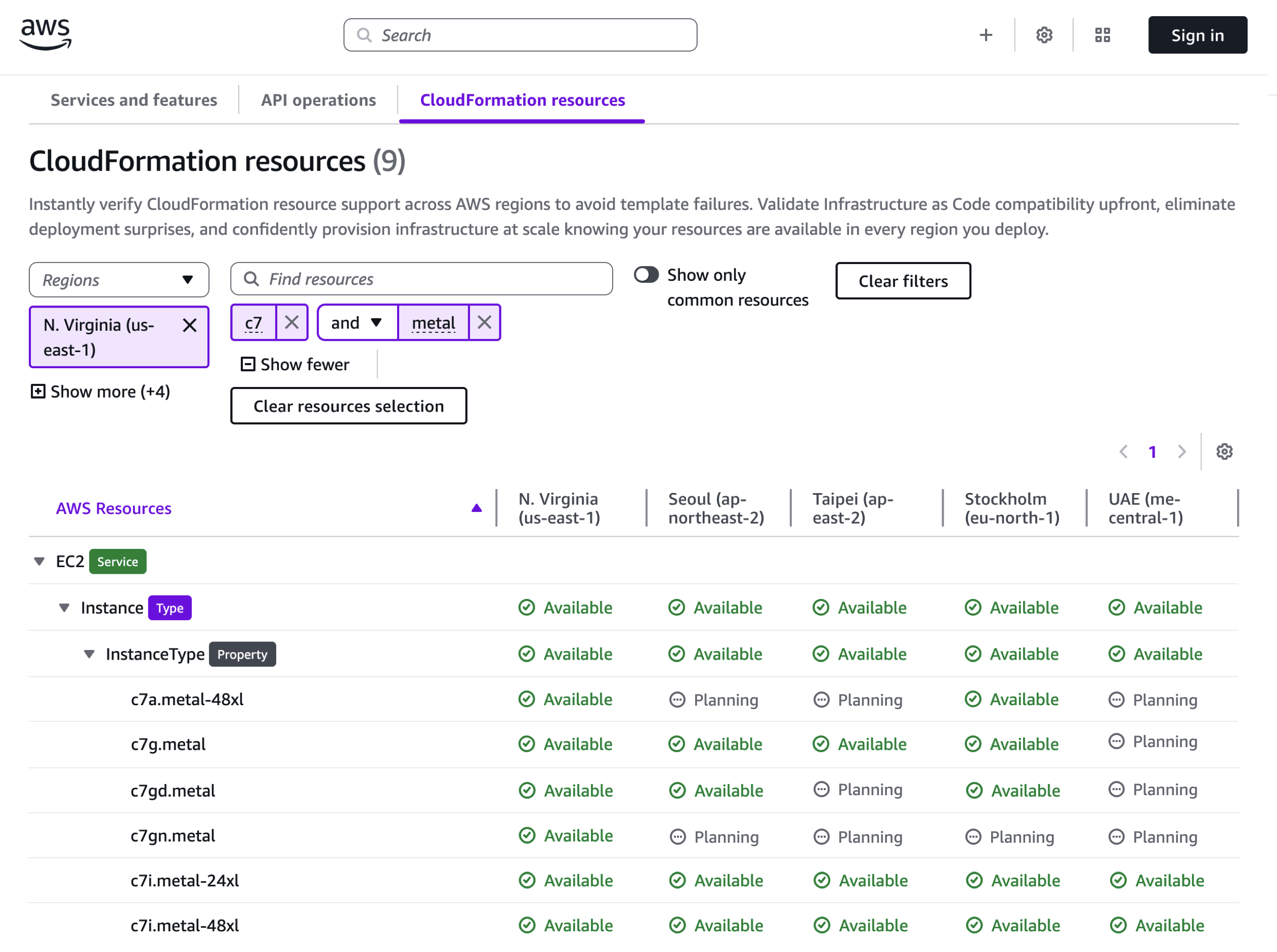
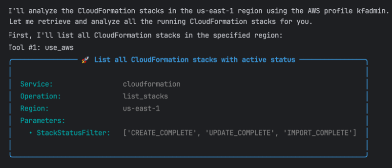
If you’re using an AI–powered assistant for software development such as Amazon Q Developer or Kiro, you can set up the AWS API MCP Server to help the AI assistants interact with AWS services and resources and the AWS Knowledge MCP Server to provide up-to-date documentation, code samples, knowledge about the regional availability of AWS APIs and CloudFormation resources.
Start building multimodal AI-powered applications with Nova Multimodal Embeddings today, and share your feedback through AWS re:Post for Amazon Bedrock or your usual AWS Support contacts.
— Danilo


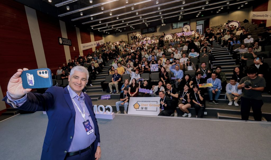 Last week I met Jeff Barr at the
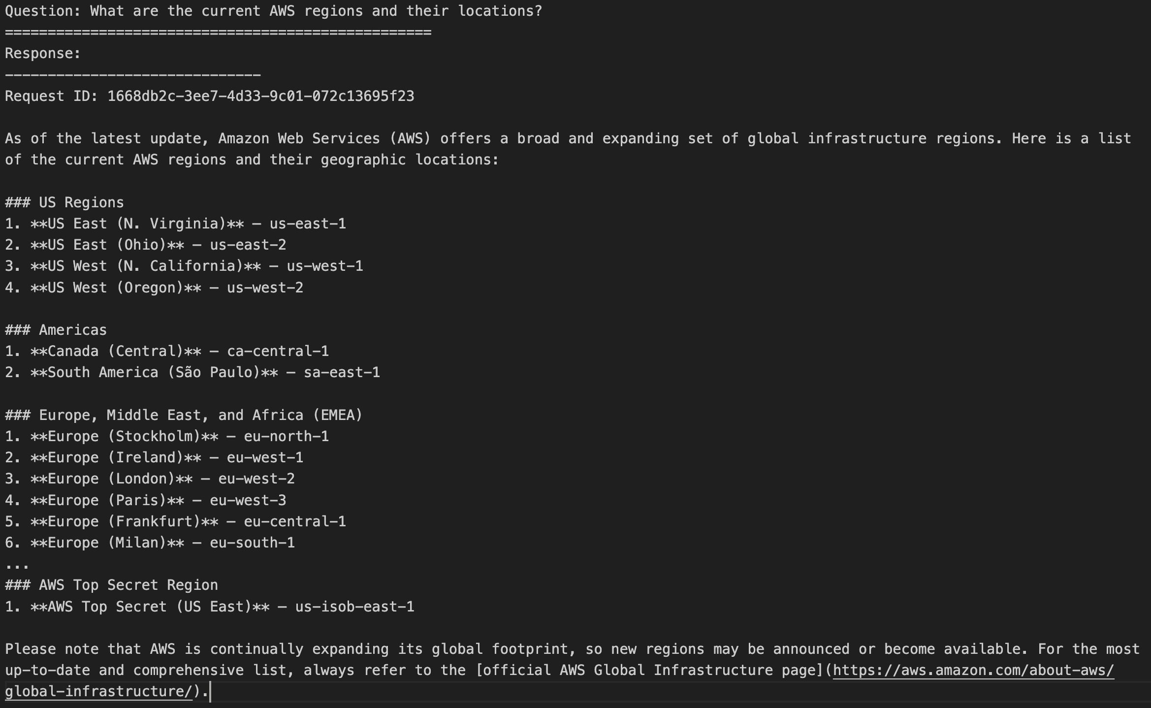


 This announcement builds upon two significant storage integration milestones we achieved in the past year. In December 2024, we introduced