Tag Archives: Amazon DocumentDB

Vector search for Amazon DocumentDB (with MongoDB compatibility) is now generally available

Post Syndicated from Channy Yun original https://aws.amazon.com/blogs/aws/vector-search-for-amazon-documentdb-with-mongodb-compatibility-is-now-generally-available/

Today, we are announcing the general availability of vector search for Amazon DocumentDB (with MongoDB compatibility), a new built-in capability that lets you store, index, and search millions of vectors with millisecond response times within your document database.

Vector search is an emerging technique used in machine learning (ML) to find similar data points to given data by comparing their vector representations using distance or similarity metrics. Vectors are numerical representation of unstructured data created from large language models (LLM) hosted in Amazon Bedrock, Amazon SageMaker, and other open source or proprietary ML services. This approach is useful in creating generative artificial intelligence (AI) applications, such as intuitive search, product recommendation, personalization, and chatbots using Retrieval Augmented Generation (RAG) model approach. For example, if your data set contained individual documents for movies, you could semantically search for movies similar to Titanic based on shared context such as “boats”, “tragedy”, or “movies based on true stories” instead of simply matching keywords.

With vector search for Amazon DocumentDB, you can effectively search the database based on nuanced meaning and context without spending time and cost to manage a separate vector database infrastructure. You also benefit from the fully managed, scalable, secure, and highly available JSON-based document database that Amazon DocumentDB provides.

Getting started with vector search on Amazon DocumentDB
The vector search feature is available on your Amazon DocumentDB 5.0 instance-based clusters. To implement a vector search application, you generate vectors using embedding models for fields inside your document and store vectors side by side your source data inside Amazon DocumentDB.

Next, you create a vector index on a vector field that will help retrieve similar vectors and can search the Amazon DocumentDB database using semantic search. Finally, user-submitted queries are converted to vectors using the same embedding model to get semantically similar documents and return them to the client.

Let’s look at how to implement a simple semantic search application using vector search on Amazon DocumentDB.

Step 1. Create vector embeddings using the Amazon Titan Embeddings model
Let’s use the Amazon Titan Embeddings model to create an embedding vector. Amazon Titan Embeddings model is available in Amazon Bedrock, a serverless generative AI service. You can easily access it using a single API and without managing any infrastructure.

prompt = "I love dog and cat."
response = bedrock_runtime.invoke_model(
    body= json.dumps({"inputText": prompt}), 
    modelId='amazon.titan-embed-text-v1', 
    accept='application/json', 
    contentType='application/json'
)
response_body = json.loads(response['body'].read())
embedding = response_body.get('embedding')

The returned vector embedding will look similar to this:

[0.82421875, -0.6953125, -0.115722656, 0.87890625, 0.05883789, -0.020385742, 0.32421875, -0.00078201294, -0.40234375, 0.44140625, ...]

Step 2. Insert vector embeddings and create a vector index
You can add generated vector embeddings using the insertMany( [{},...,{}] ) operation with a list of the documents that you want added to your collection in Amazon DocumentDB.

db.collection.insertMany([
    {sentence: "I love a dog and cat.", vectorField: [0.82421875, -0.6953125,...]},
    {sentence: "My dog is very cute.", vectorField: [0.05883789, -0.020385742,...]},
    {sentence: "I write with a pen.", vectorField: [-0.020385742, 0.32421875,...]},
  ...
]);

You can create a vector index using the createIndex command. Amazon DocumentDB performs an approximate nearest neighbor (ANN) search using the inverted file with flat compression (IVFFLAT) vector index. The feature supports three distance metrics: euclidean, cosine, and inner product. We will use the euclidean distance, a measure of the straight-line distance between two points in space. The smaller the euclidean distance, the closer the vectors are to each other.

db.collection.createIndex (
   { vectorField: "vector" },
   { "name": "index name",
     "vectorOptions": {
        "dimensions": 100, // the number of vector data dimensions
        "similarity": "euclidean", // Or cosine and dotProduct
        "lists": 100 
      }
   }
);

Step 3.  Search vector embeddings from Amazon DocumentDB
You can now search for similar vectors within your documents using a new aggregation pipeline operator within $search. The example code to search “I like pets” is as follows:

db.collection.aggregate ({
  $search: {
    "vectorSearch": {
      "vector": [0.82421875, -0.6953125,...], // Search for ‘I like pets’
      "path": vectorField,
      "k": 5,
      "similarity": "euclidean", // Or cosine and dotProduct
      "probes": 1 // the number of clusters for vector search
      }
     }
   });

This returns search results such as “I love a dog and cat.” which is semantically similar.

To learn more, see Amazon DocumentDB documentation. To see a more practical example—a semantic movie search with Amazon DocumentDB—find the Python source codes and data-sets in the GitHub repository.

Now available
Vector search for Amazon DocumentDB is now available at no additional cost to all customers using Amazon DocumentDB 5.0 instance-based clusters in all AWS Regions where Amazon DocumentDB is available. Standard compute, I/O, storage, and backup charges will apply as you store, index, and search vector embeddings on Amazon DocumentDB.

To learn more, see the Amazon DocumentDB documentation and send feedback to AWS re:Post for Amazon DocumentDB or through your usual AWS Support contacts.

Channy

Serverless ICYMI Q1 2023

Post Syndicated from Julian Wood original https://aws.amazon.com/blogs/compute/serverless-icymi-q1-2023/

Welcome to the 21st edition of the AWS Serverless ICYMI (in case you missed it) quarterly recap. Every quarter, we share all the most recent product launches, feature enhancements, blog posts, webinars, live streams, and other interesting things that you might have missed!

ICYMI2023Q1

In case you missed our last ICYMI, check out what happened last quarter here.

Artificial intelligence (AI) technologies, ChatGPT, and DALL-E are creating significant interest in the industry at the moment. Find out how to integrate serverless services with ChatGPT and DALL-E to generate unique bedtime stories for children.

Example notification of a story hosted with Next.js and App Runner

Example notification of a story hosted with Next.js and App Runner

Serverless Land is a website maintained by the Serverless Developer Advocate team to help you build serverless applications and includes workshops, code examples, blogs, and videos. There is now enhanced search functionality so you can search across resources, patterns, and video content.

SLand-search

ServerlessLand search

AWS Lambda

AWS Lambda has improved how concurrency works with Amazon SQS. You can now control the maximum number of concurrent Lambda functions invoked.

The launch blog post explains the scaling behavior of Lambda using this architectural pattern, challenges this feature helps address, and a demo of maximum concurrency in action.

Maximum concurrency is set to 10 for the SQS queue.

Maximum concurrency is set to 10 for the SQS queue.

AWS Lambda Powertools is an open-source library to help you discover and incorporate serverless best practices more easily. Lambda Powertools for .NET is now generally available and currently focused on three observability features: distributed tracing (Tracer), structured logging (Logger), and asynchronous business and application metrics (Metrics). Powertools is also available for Python, Java, and Typescript/Node.js programming languages.

To learn more:

Lambda announced a new feature, runtime management controls, which provide more visibility and control over when Lambda applies runtime updates to your functions. The runtime controls are optional capabilities for advanced customers that require more control over their runtime changes. You can now specify a runtime management configuration for each function with three settings, Automatic (default), Function update, or manual.

There are three new Amazon CloudWatch metrics for asynchronous Lambda function invocations: AsyncEventsReceived, AsyncEventAge, and AsyncEventsDropped. You can track the asynchronous invocation requests sent to Lambda functions to monitor any delays in processing and take corrective actions if required. The launch blog post explains the new metrics and how to use them to troubleshoot issues.

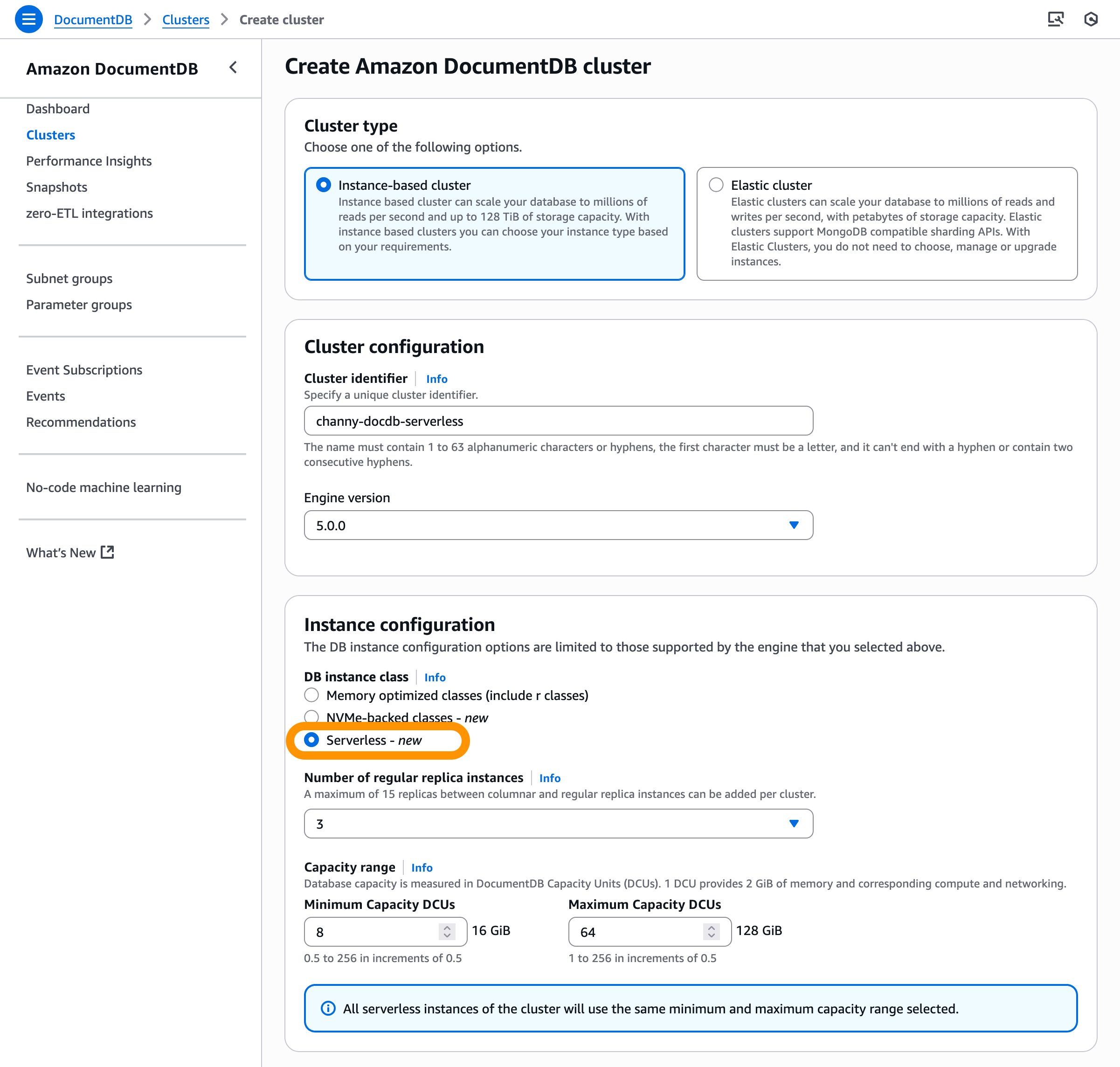
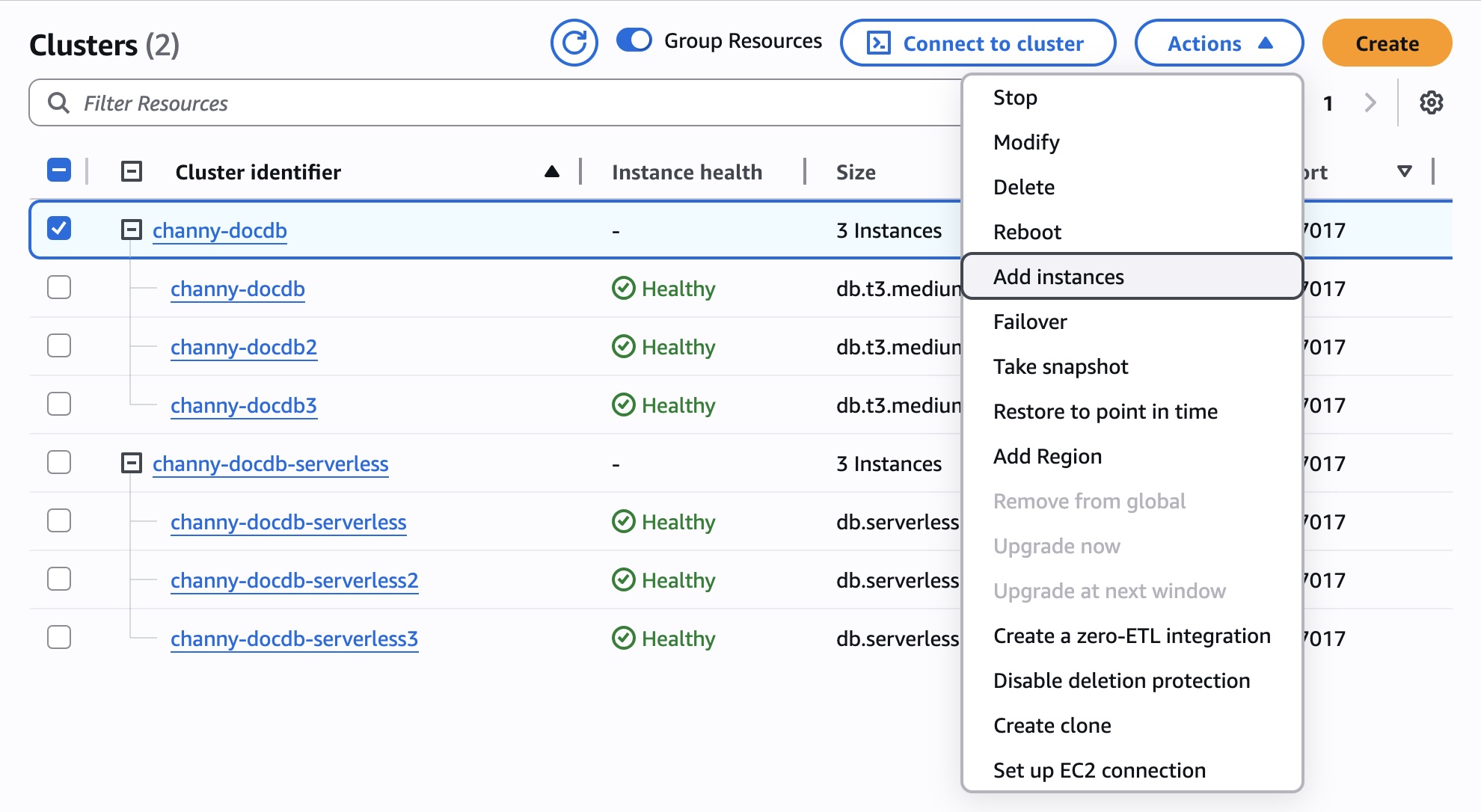
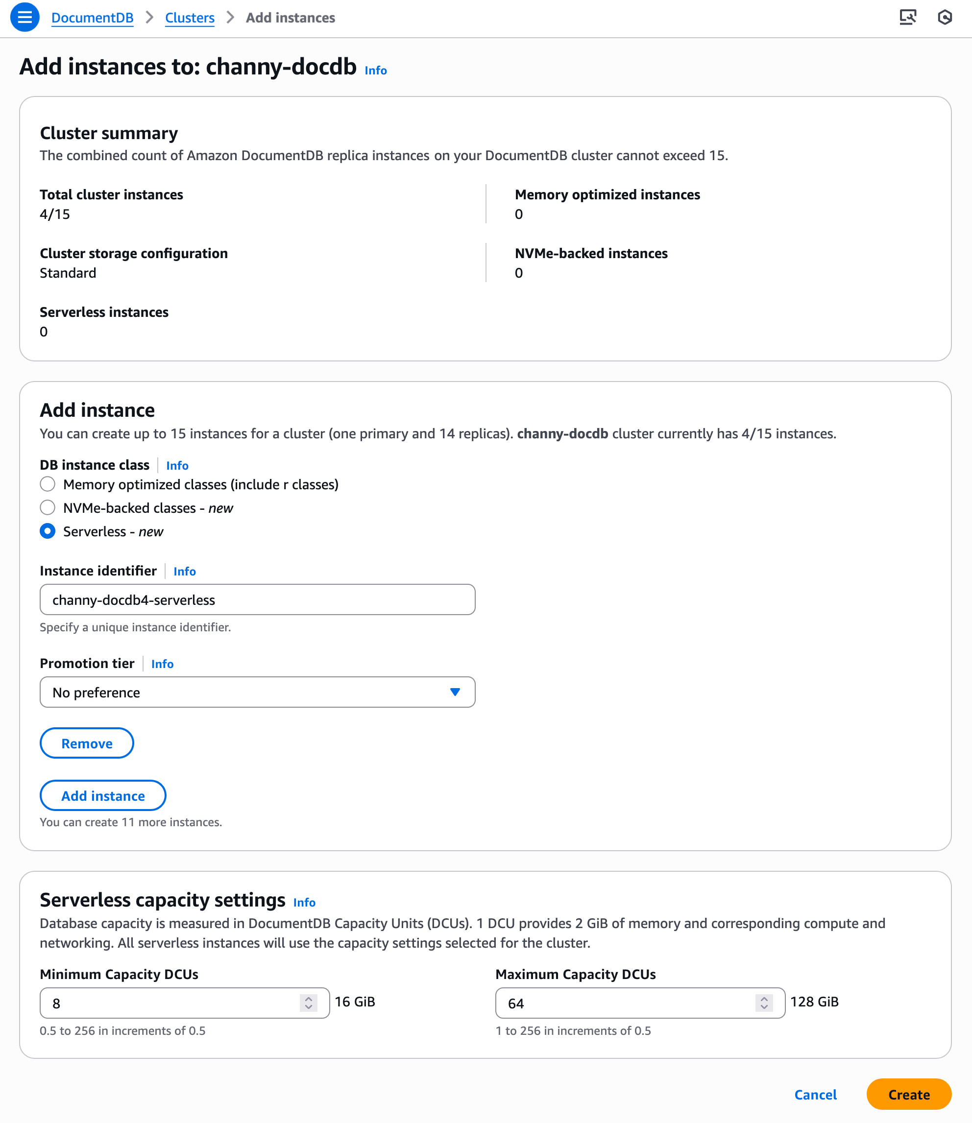
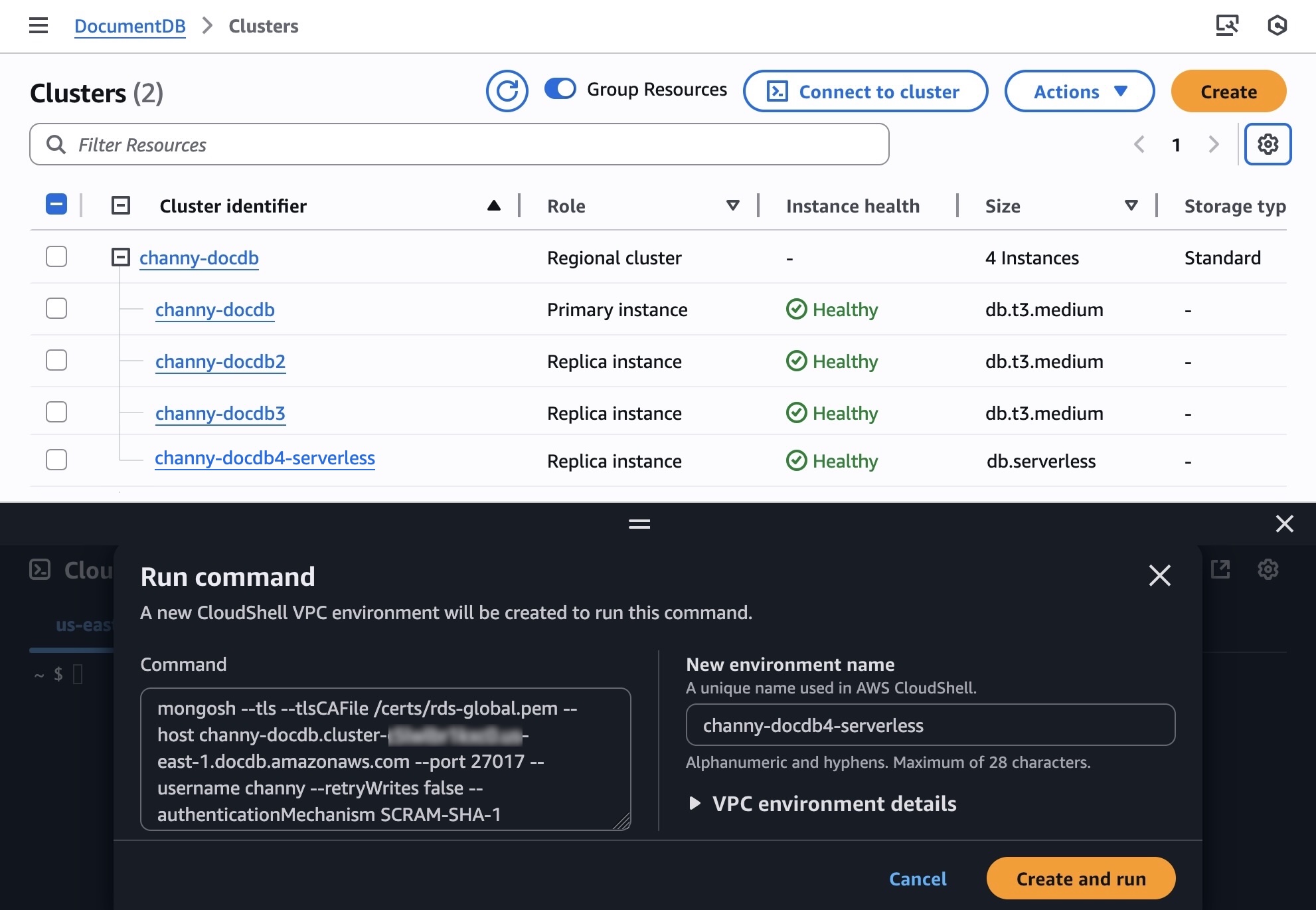
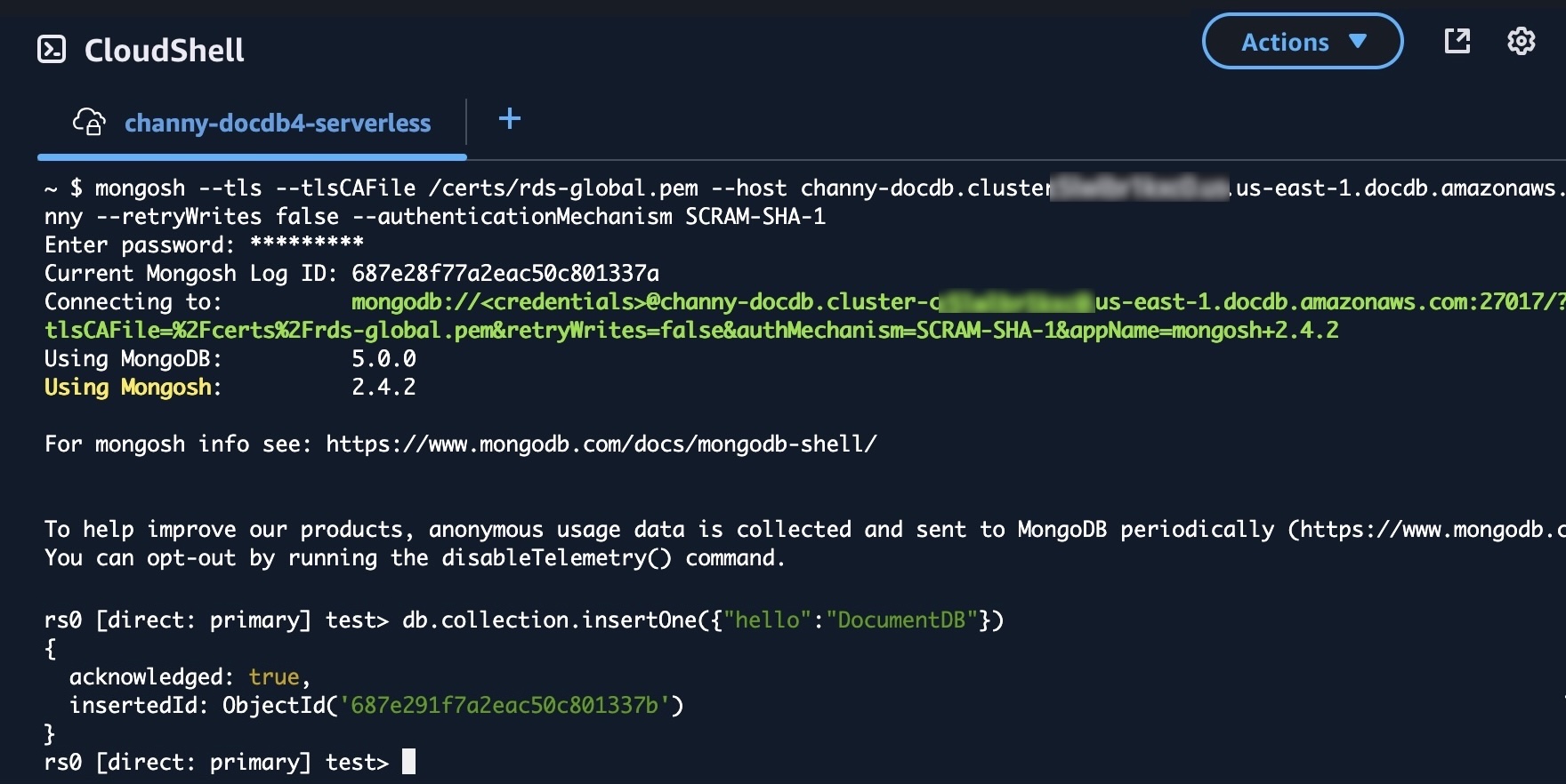
Lambda now supports Amazon DocumentDB change streams as an event source. You can use Lambda functions to process new documents, track updates to existing documents, or log deleted documents. You can use any programming language that is supported by Lambda to write your functions.

There is a helpful blog post suggesting best practices for developing portable Lambda functions that allow you to port your code to containers if you later choose to.

AWS Step Functions

AWS Step Functions has expanded its AWS SDK integrations with support for 35 additional AWS services including Amazon EMR Serverless, AWS Clean Rooms, AWS IoT FleetWise, AWS IoT RoboRunner and 31 other AWS services. In addition, Step Functions also added support for 1000+ new API actions from new and existing AWS services such as Amazon DynamoDB and Amazon Athena. For the full list of added services, visit AWS SDK service integrations.

Amazon EventBridge

Amazon EventBridge has launched the AWS Controllers for Kubernetes (ACK) for EventBridge and Pipes . This allows you to manage EventBridge resources, such as event buses, rules, and pipes, using the Kubernetes API and resource model (custom resource definitions).

EventBridge event buses now also support enhanced integration with Service Quotas. Your quota increase requests for limits such as PutEvents transactions-per-second, number of rules, and invocations per second among others will be processed within one business day or faster, enabling you to respond quickly to changes in usage.

AWS SAM

The AWS Serverless Application Model (SAM) Command Line Interface (CLI) has added the sam list command. You can now show resources defined in your application, including the endpoints, methods, and stack outputs required to test your deployed application.

AWS SAM has a preview of sam build support for building and packaging serverless applications developed in Rust. You can use cargo-lambda in the AWS SAM CLI build workflow and AWS SAM Accelerate to iterate on your code changes rapidly in the cloud.

You can now use AWS SAM connectors as a source resource parameter. Previously, you could only define AWS SAM connectors as a AWS::Serverless::Connector resource. Now you can add the resource attribute on a connector’s source resource, which makes templates more readable and easier to update over time.

AWS SAM connectors now also support multiple destinations to simplify your permissions. You can now use a single connector between a single source resource and multiple destination resources.

In October 2022, AWS released OpenID Connect (OIDC) support for AWS SAM Pipelines. This improves your security posture by creating integrations that use short-lived credentials from your CI/CD provider. There is a new blog post on how to implement it.

Find out how best to build serverless Java applications with the AWS SAM CLI.

AWS App Runner

AWS App Runner now supports retrieving secrets and configuration data stored in AWS Secrets Manager and AWS Systems Manager (SSM) Parameter Store in an App Runner service as runtime environment variables.

AppRunner also now supports incoming requests based on HTTP 1.0 protocol, and has added service level concurrency, CPU and Memory utilization metrics.

Amazon S3

Amazon S3 now automatically applies default encryption to all new objects added to S3, at no additional cost and with no impact on performance.

You can now use an S3 Object Lambda Access Point alias as an origin for your Amazon CloudFront distribution to tailor or customize data to end users. For example, you can resize an image depending on the device that an end user is visiting from.

S3 has introduced Mountpoint for S3, a high performance open source file client that translates local file system API calls to S3 object API calls like GET and LIST.

S3 Multi-Region Access Points now support datasets that are replicated across multiple AWS accounts. They provide a single global endpoint for your multi-region applications, and dynamically route S3 requests based on policies that you define. This helps you to more easily implement multi-Region resilience, latency-based routing, and active-passive failover, even when data is stored in multiple accounts.

Amazon Kinesis

Amazon Kinesis Data Firehose now supports streaming data delivery to Elastic. This is an easier way to ingest streaming data to Elastic and consume the Elastic Stack (ELK Stack) solutions for enterprise search, observability, and security without having to manage applications or write code.

Amazon DynamoDB

Amazon DynamoDB now supports table deletion protection to protect your tables from accidental deletion when performing regular table management operations. You can set the deletion protection property for each table, which is set to disabled by default.

Amazon SNS

Amazon SNS now supports AWS X-Ray active tracing to visualize, analyze, and debug application performance. You can now view traces that flow through Amazon SNS topics to destination services, such as Amazon Simple Queue Service, Lambda, and Kinesis Data Firehose, in addition to traversing the application topology in Amazon CloudWatch ServiceLens.

SNS also now supports setting content-type request headers for HTTPS notifications so applications can receive their notifications in a more predictable format. Topic subscribers can create a DeliveryPolicy that specifies the content-type value that SNS assigns to their HTTPS notifications, such as application/json, application/xml, or text/plain.

EDA Visuals collection added to Serverless Land

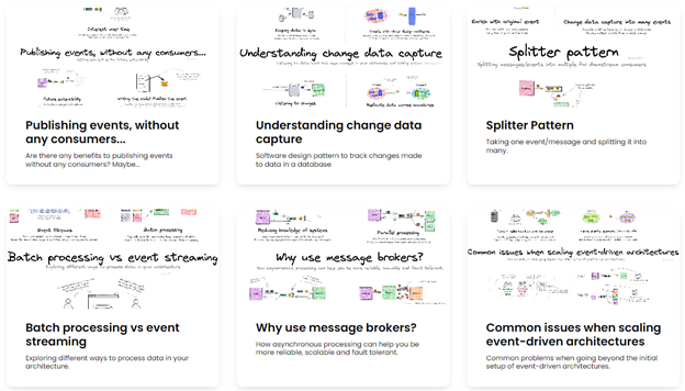
The Serverless Developer Advocate team has extended Serverless Land and introduced EDA visuals. These are small bite sized visuals to help you understand concept and patterns about event-driven architectures. Find out about batch processing vs. event streaming, commands vs. events, message queues vs. event brokers, and point-to-point messaging. Discover bounded contexts, migrations, idempotency, claims, enrichment and more!

EDA-visuals

EDA Visuals

To learn more:

Serverless Repos Collection on Serverless Land

There is also a new section on Serverless Land containing helpful code repositories. You can search for code repos to use for examples, learning or building serverless applications. You can also filter by use-case, runtime, and level.

Serverless Repos Collection

Serverless Repos Collection

Serverless Blog Posts

January

Jan 12 – Introducing maximum concurrency of AWS Lambda functions when using Amazon SQS as an event source

Jan 20 – Processing geospatial IoT data with AWS IoT Core and the Amazon Location Service

Jan 23 – AWS Lambda: Resilience under-the-hood

Jan 24 – Introducing AWS Lambda runtime management controls

Jan 24 – Best practices for working with the Apache Velocity Template Language in Amazon API Gateway

February

Feb 6 – Previewing environments using containerized AWS Lambda functions

Feb 7 – Building ad-hoc consumers for event-driven architectures

Feb 9 – Implementing architectural patterns with Amazon EventBridge Pipes

Feb 9 – Securing CI/CD pipelines with AWS SAM Pipelines and OIDC

Feb 9 – Introducing new asynchronous invocation metrics for AWS Lambda

Feb 14 – Migrating to token-based authentication for iOS applications with Amazon SNS

Feb 15 – Implementing reactive progress tracking for AWS Step Functions

Feb 23 – Developing portable AWS Lambda functions

Feb 23 – Uploading large objects to Amazon S3 using multipart upload and transfer acceleration

Feb 28 – Introducing AWS Lambda Powertools for .NET

March

Mar 9 – Server-side rendering micro-frontends – UI composer and service discovery

Mar 9 – Building serverless Java applications with the AWS SAM CLI

Mar 10 – Managing sessions of anonymous users in WebSocket API-based applications

Mar 14 –
Implementing an event-driven serverless story generation application with ChatGPT and DALL-E

Videos

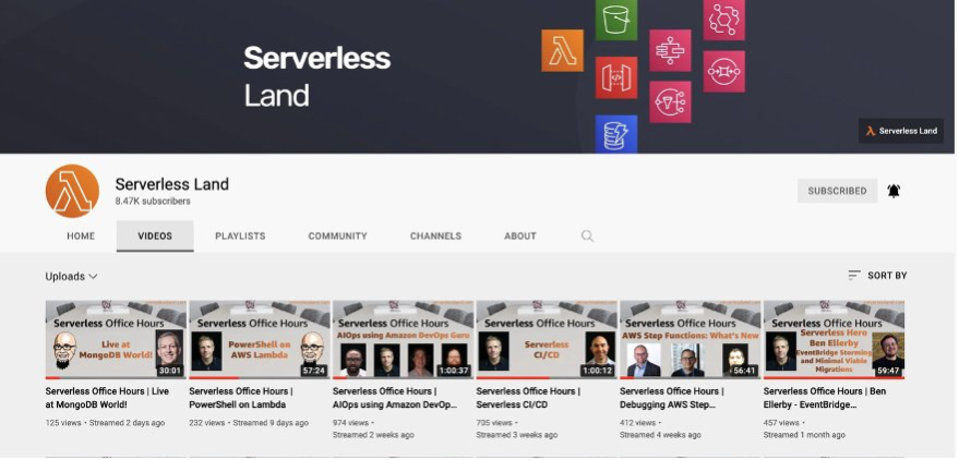
Serverless Office Hours – Tues 10AM PT

Weekly office hours live stream. In each session we talk about a specific topic or technology related to serverless and open it up to helping you with your real serverless challenges and issues. Ask us anything you want about serverless technologies and applications.

January

Jan 10 – Building .NET 7 high performance Lambda functions

Jan 17 – Amazon Managed Workflows for Apache Airflow at Scale

Jan 24 – Using Terraform with AWS SAM

Jan 31 – Preparing your serverless architectures for the big day

February

Feb 07- Visually design and build serverless applications

Feb 14 – Multi-tenant serverless SaaS

Feb 21 – Refactoring to Serverless

Feb 28 – EDA visually explained

March

Mar 07 – Lambda cookbook with Python

Mar 14 – Succeeding with serverless

Mar 21 – Lambda Powertools .NET

Mar 28 – Server-side rendering micro-frontends

FooBar Serverless YouTube channel

Marcia Villalba frequently publishes new videos on her popular serverless YouTube channel. You can view all of Marcia’s videos at https://www.youtube.com/c/FooBar_codes.

January

Jan 12 – Serverless Badge – A new certification to validate your Serverless Knowledge

Jan 19 – Step functions Distributed map – Run 10k parallel serverless executions!

Jan 26 – Step Functions Intrinsic Functions – Do simple data processing directly from the state machines!

February

Feb 02 – Unlock the Power of EventBridge Pipes: Integrate Across Platforms with Ease!

Feb 09 – Amazon EventBridge Pipes: Enrichment and filter of events Demo with AWS SAM

Feb 16 – AWS App Runner – Deploy your apps from GitHub to Cloud in Record Time

Feb 23 – AWS App Runner – Demo hosting a Node.js app in the cloud directly from GitHub (AWS CDK)

March

Mar 02 – What is Amazon DynamoDB? What are the most important concepts? What are the indexes?

Mar 09 – Choreography vs Orchestration: Which is Best for Your Distributed Application?

Mar 16 – DynamoDB Single Table Design: Simplify Your Code and Boost Performance with Table Design Strategies

Mar 23 – 8 Reasons You Should Choose DynamoDB for Your Next Project and How to Get Started

Sessions with SAM & Friends

SAMFiends

AWS SAM & Friends

Eric Johnson is exploring how developers are building serverless applications. We spend time talking about AWS SAM as well as others like AWS CDK, Terraform, Wing, and AMPT.

Feb 16 – What’s new with AWS SAM

Feb 23 – AWS SAM with AWS CDK

Mar 02 – AWS SAM and Terraform

Mar 10 – Live from ServerlessDays ANZ

Mar 16 – All about AMPT

Mar 23 – All about Wing

Mar 30 – SAM Accelerate deep dive

Still looking for more?

The Serverless landing page has more information. The Lambda resources page contains case studies, webinars, whitepapers, customer stories, reference architectures, and even more Getting Started tutorials.

You can also follow the Serverless Developer Advocacy team on Twitter to see the latest news, follow conversations, and interact with the team.

Announcing Amazon DocumentDB Elastic Clusters

Post Syndicated from Veliswa Boya original https://aws.amazon.com/blogs/aws/announcing-amazon-documentdb-elastic-clusters/

Amazon DocumentDB (with MongoDB compatibility) is a scalable, highly durable, and fully managed database service for operating mission-critical JSON workloads. It is one of AWS fast-growing services with customers including BBC, Dow Jones, and Samsung relying on Amazon DocumentDB to run their JSON workloads at scale.

Today I am excited to announce the general availability of Amazon DocumentDB Elastic Clusters. Elastic Clusters enables you to elastically scale your document database to handle virtually any number of writes and reads, with petabytes of storage capacity. Elastic Clusters simplifies how customers interact with Amazon DocumentDB by automatically managing the underlying infrastructure and removing the need to create, remove, upgrade, or scale instances.

A Few Concepts about Elastic Clusters
Sharding – A popular database concept also known as partitioning, sharding splits large data sets into smaller data sets across multiple nodes enabling customers to scale out their database beyond vertical scaling limits. Elastic Clusters uses sharding to partition data across Amazon DocumentDB’s distributed storage system. 

Elastic Clusters – Elastic Clusters is Amazon DocumentDB clusters that allow you to scale your workload’s throughput to millions of writes/reads per second and storage to petabytes. Elastic Clusters comprises one or more shards each of which has its own compute and storage volume. It is highly available across three Availability Zones (AZs) by default, with six copies of your data replicated across these three AZs. You can create Elastic Clusters using the Amazon DocumentDB API, AWS SDK, AWS CLI, AWS CloudFormation, or the AWS console.

Scale Workloads with Little to No Impact – With Elastic Clusters, your database can scale to millions of operations with little to no downtime or performance impact.

Integration with Other AWS Services – Elastic Clusters integrates with other AWS services in the same way Amazon DocumentDB does today. First, you can monitor the health and performance of your Elastic Clusters using Amazon CloudWatch. Second, you can set up authentication and authorization for resources such as clusters through AWS Identity and Access Management (IAM) users and roles and use Amazon Virtual Private Cloud (Amazon VPC) for secure VPC-only connections. Last, you can use AWS Glue to import and export data from and to other AWS services such as Amazon Simple Storage Service (Amazon S3), Amazon Redshift, and Amazon OpenSearch Service.

Getting Started with Elastic Clusters
Previously, I mentioned that you can use either the AWS console, AWS CLI, or AWS SDK to create Elastic Clusters. In the examples below, we will look at how you can create a cluster, scale up or out, and scale in or down using the AWS CLI:

Create a Cluster
When creating a cluster, you will specify the vCPUs that you want for your Elastic Clusters at provisioning. With the size of vCPUs that you provision, you will also get a proportionate amount of memory, expressed in vCPUs. Elastic Clusters automatically provisions the necessary infrastructure (shards and instances) on your behalf.
aws docdb-elastic create-cluster
--cluster-name foo
--shard-capacity 2
--shard-count 4
--auth-type PLAIN_TEXT
--admin-user-name docdbelasticadmin
--admin-user-password password

Scale Up or Out
If you need more compute and storage to handle an increase in traffic, modify the shard-count parameter. Elastic Clusters scales the underlying infrastructure up or out to give you additional compute and storage capacity.
aws docdb-elastic update-cluster
--cluster-arn foo-arn
--shard-count 8

Scale In or Down
If you no longer need the compute and storage that you currently have provisioned, either due to a decline in database traffic or the fact that you originally over-provisioned, modify the shard-count parameter. Elastic Clusters scales the underlying infrastructure in or down.
aws docdb-elastic update-cluster
--cluster-arn foo-arn
--shard-count 4

General Availability of Elastic Clusters for Amazon DocumentDB
Amazon DocumentDB Elastic Clusters is now available in all AWS Regions where Amazon DocumentDB is available, except China and AWS GovCloud. To learn more, visit the Amazon DocumentDB page.

Veliswa x

Creating a Multi-Region Application with AWS Services – Part 2, Data and Replication

Post Syndicated from Joe Chapman original https://aws.amazon.com/blogs/architecture/creating-a-multi-region-application-with-aws-services-part-2-data-and-replication/

In Part 1 of this blog series, we looked at how to use AWS compute, networking, and security services to create a foundation for a multi-Region application.

Data is at the center of many applications. In this post, Part 2, we will look at AWS data services that offer native features to help get your data where it needs to be.

In Part 3, we’ll look at AWS application management and monitoring services to help you build, monitor, and maintain a multi-Region application.

Considerations with replicating data

Data replication across the AWS network can happen quickly, but we are still limited by the speed of light. For this reason, data consistency must be considered when building a multi-Region application. Generally speaking, the longer a physical distance is, the longer it will take the data to get there.

When building a distributed system, consider the consistency, availability, partition tolerance (CAP) theorem. This theorem states that an application can only pick 2 out of the 3, and tradeoffs should be considered.

  • Consistency – all clients always have the same view of data
  • Availability – all clients can always read and write data
  • Partition Tolerance – the system will continue to work despite physical partitions

CAP diagram

Achieving consistency and availability is common for single-Region applications. For example, when an application connects to a single in-Region database. However, this becomes more difficult with multi-Region applications due to the latency added by transferring data over long distances. For this reason, highly distributed systems will typically follow an eventual consistency approach, favoring availability and partition tolerance.

Replicating objects and files

To ensure objects are in multiple Regions, Amazon Simple Storage Service (Amazon S3) can be set up to replicate objects across AWS Regions automatically with one-way or two-way replication. A subset of objects in an S3 bucket can be replicated with S3 replication rules. If low replication lag is critical, S3 Replication Time Control can help meet requirements by replicating 99.99% of objects within 15 minutes, and most within seconds. To monitor the replication status of objects, Amazon S3 events and metrics will track replication and can send an alert if there’s an issue.

Traditionally, each S3 bucket has its own single, Regional endpoint. To simplify connecting to and managing multiple endpoints, S3 Multi-Region Access Points create a single global endpoint spanning multiple S3 buckets in different Regions. When applications connect to this endpoint, it will route over the AWS network using AWS Global Accelerator to the bucket with the lowest latency. Failover routing is also automatically handled if the connectivity or availability to a bucket changes.

For files stored outside of Amazon S3, AWS DataSync simplifies, automates, and accelerates moving file data across Regions and accounts. It supports homogeneous and heterogeneous file migrations across Elastic File System (Amazon EFS), Amazon FSx, AWS Snowcone, and Amazon S3. It can even be used to sync on-premises files stored on NFS, SMB, HDFS, and self-managed object storage to AWS for hybrid architectures.

File and object replication should be expected to be eventually consistent. The rate at which a given dataset can transfer is a function of the amount of data, I/O bandwidth, network bandwidth, and network conditions.

Copying backups

Scheduled backups can be set up with AWS Backup, which automates backups of your data to meet business requirements. Backup plans can automate copying backups to one or more AWS Regions or accounts. A growing number of services are supported, and this can be especially useful for services that don’t offer real-time replication to another Region such as Amazon Elastic Block Store (Amazon EBS) and Amazon Neptune.

Figure 1 shows how these data transfer services can be combined for each resource.

Storage replication services

Figure 1. Storage replication services

Spanning non-relational databases across Regions

Amazon DynamoDB global tables provide multi-Region and multi-writer features to help you build global applications at scale. A DynamoDB global table is the only AWS managed offering that allows for multiple active writers in a multi-Region topology (active-active and multi-Region). This allows for applications to read and write in the Region closest to them, with changes automatically replicated to other Regions.

Global reads and fast recovery for Amazon DocumentDB (with MongoDB compatibility) can be achieved with global clusters. These clusters have a primary Region that handles write operations. Dedicated storage-based replication infrastructure enables low-latency global reads with a lag of typically less than one second.

Keeping in-memory caches warm with the same data across Regions can be critical to maintain application performance. Amazon ElastiCache for Redis offers global datastore to create a fully managed, fast, reliable, and secure cross-Region replica for Redis caches and databases. With global datastore, writes occurring in one Region can be read from up to two other cross-Region replica clusters – eliminating the need to write to multiple caches to keep them warm.

Spanning relational databases across Regions

For applications that require a relational data model, Amazon Aurora global database provides for scaling of database reads across Regions in Aurora PostgreSQL-compatible and MySQL-compatible editions. Dedicated replication infrastructure utilizes physical replication to achieve consistently low replication lag that outperforms the built-in logical replication database engines offer, as shown in Figure 2.

SysBench OLTP (write-only) stepped every 600 seconds on R4.16xlarge

Figure 2. SysBench OLTP (write-only) stepped every 600 seconds on R4.16xlarge

With Aurora global database, one primary Region is designated as the writer, and secondary Regions are dedicated to reads. Aurora MySQL supports write forwarding, which forwards write requests from a secondary Region to the primary Region to simplify logic in application code. Failover testing can happen by utilizing managed planned failover, which will change the active write cluster to another Region while keeping the replication topology intact. All databases discussed in this post employ eventual consistency when used across Regions, but Aurora PostgreSQL has an option to set the maximum a replica lag allowed with managed recovery point objective (managed RPO).

Logical replication, which utilizes a database engine’s built-in replication technology, can be set up for Amazon Relational Database Service (Amazon RDS) for MariaDB, MySQL, Oracle, PostgreSQL, and Aurora databases. A cross-Region read replica will receive these changes from the writer in the primary Region. For applications built on RDS for Microsoft SQL Server, cross-Region replication can be achieved by utilizing the AWS Database Migration Service. Cross-Region replicas allow for quicker local reads and can reduce data loss and recovery times in the case of a disaster by being promoted to a standalone instance.

For situations where a longer RPO and recovery time objective (RTO) are acceptable, backups can be copied across Regions. This is true for all of the relational and non-relational databases mentioned in this post, except for ElastiCache for Redis. Amazon Redshift can also automatically do this for your data warehouse. Backup copy times will vary depending on size and change rates.

A purpose-built database strategy offers many benefits, Figure 3 forms a purpose-built global database architecture.

Purpose-built global database architecture

Figure 3. Purpose-built global database architecture

Summary

Data is at the center of almost every application. In this post, we reviewed AWS services that offer cross-Region data replication to get your data where it needs to be quickly. Whether you need faster local reads, an active-active database, or simply need your data durably stored in a second Region, we have a solution for you. In the 3rd and final post of this series, we’ll cover application management and monitoring features.

Ready to get started? We’ve chosen some AWS Solutions, AWS Blogs, and Well-Architected labs to help you!

Related posts

Exploring Data Transfer Costs for AWS Managed Databases

Post Syndicated from Dennis Schmidt original https://aws.amazon.com/blogs/architecture/exploring-data-transfer-costs-for-aws-managed-databases/

When selecting managed database services in AWS, it’s important to understand how data transfer charges are calculated – whether it’s relational, key-value, document, in-memory, graph, time series, wide column, or ledger.

This blog will outline the data transfer charges for several AWS managed database offerings to help you choose the most cost-effective setup for your workload.

This blog illustrates pricing at the time of publication and assumes no volume discounts or applicable taxes and duties. For demonstration purposes, we list the primary AWS Region as US East (Northern Virginia) and the secondary Region is US West (Oregon). Always refer to the individual service pricing pages for the most up-to-date pricing.

Data transfer between AWS and internet

There is no charge for inbound data transfer across all services in all Regions. When you transfer data from AWS resources to the internet, you’re charged per service, with rates specific to the originating Region. Figure 1 illustrates data transfer charges that accrue from AWS services discussed in this blog out to the public internet in the US East (Northern Virginia) Region.

Data transfer to the internet

Figure 1. Data transfer to the internet

The remainder of this blog will focus on data transfer within AWS.

Data transfer with Amazon RDS

Amazon Relational Database Service (Amazon RDS) makes it straightforward to set up, operate, and scale a relational database in the cloud. Amazon RDS provides six database engines to choose from: Amazon Aurora, MySQL, MariaDB, Oracle, SQL Server, and PostgreSQL.

Let’s consider an application running on Amazon Elastic Compute Cloud (Amazon EC2) that uses Amazon RDS as a data store.

Figure 2 illustrates where data transfer charges apply. For clarity, we have left out connection points to the replica servers – this is addressed in Figure 3.

Amazon RDS data transfer

Figure 2. Amazon RDS data transfer

In this setup, you will not incur charges for:

  • Data transfer to or from Amazon EC2 in the same Region, Availability Zone, and virtual private cloud (VPC)

You will accrue charges for data transfer between:

  • Amazon EC2 and Amazon RDS across Availability Zones within the same VPC, charged at Amazon EC2 and Amazon RDS ($0.01/GB in and $0.01/GB out)
  • Amazon EC2 and Amazon RDS across Availability Zones and across VPCs, charged at Amazon EC2 only ($0.01/GB in and $0.01/GB out). For Aurora, this is charged at Amazon EC2 and Aurora ($0.01/GB in and $0.01/GB out)
  • Amazon EC2 and Amazon RDS across Regions, charged on both sides of the transfer ($0.02/GB out)

Figure 3 illustrates several features that are available within Amazon RDS to show where data transfer charges apply. These include multi-Availability Zone deployment, read replicas, and cross-Region automated backups. Not all database engines support all features, consult the product documentation to learn more.

Amazon RDS features

Figure 3. Amazon RDS features

In this setup, you will not incur data transfer charges for:

In addition to the charges you will incur when you transfer data to the internet, you will accrue data transfer charges for:

  • Data replication to read replicas deployed across Regions ($0.02/GB out)
  • Regional transfers for Amazon RDS snapshot copies or automated cross-Region backups ($0.02/GB out)

Refer to the following pricing pages for more detail:

Data transfer with Amazon DynamoDB

Amazon DynamoDB is a key-value and document database that delivers single-digit millisecond performance at any scale. Figures 4 and 5 illustrate an application hosted on Amazon EC2 that uses DynamoDB as a data store and includes DynamoDB global tables and DynamoDB Accelerator (DAX).

DynamoDB with global tables

Figure 4. DynamoDB with global tables

DynamoDB without global tables

Figure 5. DynamoDB without global tables

You will not incur data transfer charges for:

  • Inbound data transfer to DynamoDB
  • Data transfer between DynamoDB and Amazon EC2 in the same Region
  • Data transfer between Amazon EC2 and DAX in the same Availability Zone

In addition to the charges you will incur when you transfer data to the internet, you will accrue charges for data transfer between:

  • Amazon EC2 and DAX across Availability Zones, charged at the EC2 instance ($0.01/GB in and $0.01/GB out)
  • Global tables for cross-Region replication or adding replicas to tables that contain data in DynamoDB, charged at the source Region, as shown in Figure 4 ($0.02/GB out)
  • Amazon EC2 and DynamoDB across Regions, charged on both sides of the transfer, as shown in Figure 5 ($0.02/GB out)

Refer to the DynamoDB pricing page for more detail.

Data transfer with Amazon Redshift

Amazon Redshift is a cloud data warehouse that makes it fast and cost-effective to analyze your data using standard SQL and your existing business intelligence tools. There are many integrations and services available to query and visualize data within Amazon Redshift. To illustrate data transfer costs, Figure 6 shows an EC2 instance running a consumer application connecting to Amazon Redshift over JDBC/ODBC.

Amazon Redshift data transfer

Figure 6. Amazon Redshift data transfer

You will not incur data transfer charges for:

  • Data transfer within the same Availability Zone
  • Data transfer to Amazon S3 for backup, restore, load, and unload operations in the same Region

In addition to the charges you will incur when you transfer data to the internet, you will accrue charges for the following:

  • Across Availability Zones, charged on both sides of the transfer ($0.01/GB in and $0.01/GB out)
  • Across Regions, charged on both sides of the transfer ($0.02/GB out)

Refer to the Amazon Redshift pricing page for more detail.

Data transfer with Amazon DocumentDB

Amazon DocumentDB (with MongoDB compatibility) is a database service that is purpose-built for JSON data management at scale. Figure 7 illustrates an application hosted on Amazon EC2 that uses Amazon DocumentDB as a data store, with read replicas in multiple Availability Zones and cross-Region replication for Amazon DocumentDB Global Clusters.

Amazon DocumentDB data transfer

Figure 7. Amazon DocumentDB data transfer

You will not incur data transfer charges for:

  • Data transfer between Amazon DocumentDB and EC2 instances in the same Availability Zone
  • Data transferred for replicating multi-Availability Zone deployments of Amazon DocumentDB between Availability Zones in the same Region

In addition to the charges you will incur when you transfer data to the internet, you will accrue charges for the following:

  • Between Amazon EC2 and Amazon DocumentDB in different Availability Zones within a Region, charged at Amazon EC2 and Amazon DocumentDB ($0.01/GB in and $0.01/GB out)
  • Across Regions between Amazon DocumentDB instances, charged at the source Region ($0.02/GB out)

Refer to the Amazon DocumentDB pricing page for more details.

Tips to save on data transfer costs to your databases

  • Review potential data transfer charges on both sides of your communication channel. Remember that “Data Transfer In” to a destination is also “Data Transfer Out” from a source.
  • Use Regional and global readers or replicas where available. This can reduce the amount of cross-Availability Zone or cross-Region traffic.
  • Consider data transfer tiered pricing when estimating workload pricing. Rate tiers aggregate usage for data transferred out to the Internet across Amazon EC2, Amazon RDS, Amazon Redshift, DynamoDB, Amazon S3, and several other services. See the Amazon EC2 On-Demand pricing page for more details.
  • Understand backup or snapshots requirements and how data transfer charges apply.
  • AWS offers various purpose-built, managed database offerings. Selecting the right one for your workload can optimize performance and cost.
  • Review your application and query design. Look for ways to reduce the amount of data transferred between your application and data store. Consider designing your application or queries to use read replicas.

Conclusion/next steps

AWS offers purpose-built databases to support your applications and data models, including relational, key-value, document, in-memory, graph, time series, wide column, and ledger databases. Each database has different deployment options, and understanding different data transfer charges can help you design a cost-efficient architecture.

This blog post is intended to help you make informed decisions for designing your workload using managed databases in AWS. Note that service charges and charges related to network topology, such as AWS Transit Gateway, VPC Peering, and AWS Direct Connect, are out of scope for this blog but should be carefully considered when designing any architecture.

Looking for more cost saving tips and information? Check out the Overview of Data Transfer Costs for Common Architectures blog post.

Zurich Spain: Managing millions of documents with AWS

Post Syndicated from Miguel Guillot original https://aws.amazon.com/blogs/architecture/zurich-spain-managing-millions-of-documents-with-aws/

This post was cowritten with Oscar Gali, Head of Technology and Architecture for GI in Zurich, Spain

About Zurich Spain

Zurich Spain is part of Zurich Insurance Group (Zurich), known for its financial soundness and solvency. With more than 135 years of history and over 2,000 employees, it is a leading company in the Spanish insurance market.

Introduction

Enterprise Content Management (ECM) is a key capability for business operations in Insurance, due to the number of documents that must be managed every day. In our digital world, managing and storing business documents and images (such as policies or claims) in a secure, available, scalable, and performant platform is critical.

Zurich Spain decided to use AWS to streamline management of their underlying infrastructure, in addition to the pay-as-you-go pricing model and advanced analytics services. All of these service features create a huge advantage for the company.

The challenge

Zurich Spain was managing all documents for non-life insurance on an on-premises proprietary solution. This was based on an ECM market standard product and specific storage infrastructure. That solution over time had several pain points: cost, scalability, and flexibility. This platform has become obsolete and was an obstacle for covering future analytical needs.

After considering different alternatives, Zurich Spain decided to base their new ECM platform on AWS, leveraging many of the managed services. AWS Managed Services helps to reduce your operational overhead and risk. AWS Managed Services automates common activities, such as change requests, monitoring, patch management, security, and backup services. It provides full lifecycle services to provision, run, and support your infrastructure.

Although the architecture design was clear, the challenge was huge. Zurich Spain had to integrate all the existing business applications with the new ECM platform. Concurrently, the company needed to migrate up to 150 million documents including metadata, in less than 6 months.

The Platform

Functionally, features provided by ECM are:

ECM Features

ECM Features

  • Authentication: every request must come from an authenticated user (OpenID Connect JWT).
  • Authorization: on every request, appropriate user permissions are validated.
  • Documentation Services: exposed API that allows interaction with documents (CRUD). For example:
    • The ability to Ingest a document either synchronously (attaching the document to the request) or asynchronously (providing a link to the requester that can be used to attach a document when required).
    • Upload operation stores documents onto Amazon Simple Storage Service (S3) and its metadata, which is saved using Amazon DocumentDB.
    • Documents Retrieve, similarly to the upload operation, can be obtained either synchronously or asynchronously. The latter provides a link to be used to download the document within a time range.
    • ECM has been developed to give the users the ability to search among all the documents uploaded into it.
  • Metadata: every document has technical and business metadata. This gives Zurich Spain the ability to enrich every single document with all the information that is relevant for their business, for example: Customers, Author, Date of creation.
  • Record Management: policies to manage documents lifecycle.
  • Audit: every transaction is logged into the system.
  • Observability: capabilities to monitor and operate all services involved: logging, performance metrics and transactions traceability.

The Architecture

The ECM platform uses AWS services such as Amazon S3 to store documents. In addition, it uses Amazon DocumentDB to store document metadata and audit trail.

The rationale for choosing these services was:

  • Amazon S3 delivers strong read-after-write consistency automatically for all applications, without changes to performance or availability. With strong consistency, Amazon S3 simplifies the migration of on-premises analytics workloads by removing the need to update applications. This reduces costs by removing the need for extra infrastructure to provide strong consistency.
  • Amazon DocumentDB is a NoSQL document-oriented database where its schema flexibility accommodates the different metadata needs. It was key to design the index strategy in advance to ensure the right query performance, considering the volume of data.

A microservices layer has been built on top to provide the right services for the business applications. These include access control, storing or retrieving documents, metadata, and more.

These microservices are built using Thunder, the internal framework and technology stack for digital applications of Zurich Spain. Thunder leverages AWS and provides a K8s environment based on Amazon Elastic Kubernetes Service (Amazon EKS) for microservice deployment.

Zurich Spain Architecture

Figure 2 – Zurich Spain Architecture

Zurich Spain uses AWS Direct Connect to connect from their data center to AWS. With AWS Direct Connect, Zurich Spain can connect to all their AWS resources in an AWS Region. They can transfer their business-critical data directly from their data center into and from AWS. This enables them to bypass their internet service provider and remove network congestion.

Amazon EKS gives Zurich Spain the flexibility to start, run, and scale Kubernetes applications in the AWS Cloud or on-premises. Amazon EKS is helping Zurich Spain to provide highly available and secure clusters while automating key tasks such as patching, node provisioning, and updates. Zurich Spain is also using Amazon Elastic Container Registry (Amazon ECR) to store, manage, share, and deploy container images and artifacts across their environment.

Some interesting metrics of the migration and platform:

  • Volume: 150+ millions (25 TB) of documents migrated
  • Duration: migration took 4 months due to the limited extraction throughput of the old platform
  • Activity: 50,000+ documents are ingested and 25,000+ retrieved daily
  • Average response time:
    • 550 ms to upload a document
    • 300 ms for retrieving a document hosted in the platform

Conclusion

Zurich Spain successfully replaced a market standard ECM product with a new flexible, highly available, and scalable ECM. This resulted in a 65% run cost reduction, improved performance, and enablement of AWS analytical services.

In addition, Zurich Spain has taken advantage of many benefits that AWS brings to their customers. They’ve demonstrated that Thunder, the new internal framework developed using AWS technology, provides fast application development with secure and frequent deployments.

Building AWS Glue Spark ETL jobs using Amazon DocumentDB (with MongoDB compatibility) and MongoDB

Post Syndicated from Naresh Gautam original https://aws.amazon.com/blogs/big-data/building-aws-glue-spark-etl-jobs-using-amazon-documentdb-with-mongodb-compatibility-and-mongodb/

AWS Glue is a fully managed extract, transform, and load (ETL) service that makes it easy to prepare and load your data for analytics. AWS Glue has native connectors to connect to supported data sources on AWS or elsewhere using JDBC drivers. Additionally, AWS Glue now supports reading and writing to Amazon DocumentDB (with MongoDB compatibility) and MongoDB collections using AWS Glue Spark ETL jobs. This feature enables you to connect and read, transform, and load (write) data from and to Amazon DocumentDB and MongoDB collections into services such as Amazon Simple Storage Service (Amazon S3) and Amazon Redshift for downstream analytics. For more information, see Connection Types and Options for ETL in AWS Glue.

This post shows how to build AWS Glue ETL Spark jobs and set up connections with Amazon DocumentDB or MongoDB to read and load data using ConnectionType. The following diagram illustrates the three components of the solution architecture:

The following diagram illustrates the three components of the solution architecture:

Prerequisites

Before getting started, you must complete the following prerequisites:

  1. Create an AWS Identity and Access Management (IAM) user with sufficient permissions to interact with the AWS Management Console. Your IAM permissions must also include access to create IAM roles and policies created by the AWS CloudFormation template provided in this post.
  2. Create an IAM policy for AWS Glue.
  3. Save the following code as DocumentDB-Glue-ETL.py in your S3 bucket.
    import sys
    from awsglue.transforms import *
    from awsglue.utils import getResolvedOptions
    from pyspark.context import SparkContext, SparkConf
    from awsglue.context import GlueContext
    from awsglue.job import Job
    import time
    
    ## @params: [JOB_NAME]
    args = getResolvedOptions(sys.argv, ['JOB_NAME'])
    
    sc = SparkContext()
    glueContext = GlueContext(sc)
    spark = glueContext.spark_session
    
    job = Job(glueContext)
    job.init(args['JOB_NAME'], args)
    
    output_path = "s3://<bucket>/<folder>/" + str(time.time()) + "/"
    documentdb_uri = "mongodb://<host name>:27017"
    documentdb_write_uri = "mongodb://<host name>:27017"
    
    read_docdb_options = {
        "uri": documentdb_uri,
        "database": "test",
        "collection": "profiles",
        "username": "<username>",
        "password": "<password>",
        "ssl": "true",
        "ssl.domain_match": "false",
        "partitioner": "MongoSamplePartitioner",
        "partitionerOptions.partitionSizeMB": "10",
        "partitionerOptions.partitionKey": "_id"
    }
    
    write_documentdb_options = {
        "uri": documentdb_write_uri,
        "database": "test",
        "collection": "collection1",
        "username": "<username>",
        "password": "<password>",
        "ssl": "true",
        "ssl.domain_match": "false",
        "partitioner": "MongoSamplePartitioner",
        "partitionerOptions.partitionSizeMB": "10",
        "partitionerOptions.partitionKey": "_id"
    }
    
    # Get DynamicFrame from DocumentDB
    dynamic_frame2 = glueContext.create_dynamic_frame.from_options(connection_type="documentdb",
                                                                   connection_options=read_docdb_options)
    
    # Write DynamicFrame to DocumentDB
    glueContext.write_dynamic_frame.from_options(dynamic_frame2, connection_type="documentdb",
                                                 connection_options=write_documentdb_options)
    
    job.commit()

  1. Save the following code as MongoDB-Glue-ETL.py in your S3 bucket.
    import sys
    from awsglue.transforms import *
    from awsglue.utils import getResolvedOptions
    from pyspark.context import SparkContext, SparkConf
    from awsglue.context import GlueContext
    from awsglue.job import Job
    import time
    
    ## @params: [JOB_NAME]
    args = getResolvedOptions(sys.argv, ['JOB_NAME'])
    
    sc = SparkContext()
    glueContext = GlueContext(sc)
    spark = glueContext.spark_session
    
    job = Job(glueContext)
    job.init(args['JOB_NAME'], args)
    
    output_path = "s3://<bucket>/<folder>/" + str(time.time()) + "/"
    mongo_uri = "mongodb://<host name or IP>:27017"
    write_uri = "mongodb://<host name or IP>:27017"
    
    read_mongo_options = {
        "uri": mongo_uri,
        "database": "test",
        "collection": "profiles",
        "username": "<username>",
        "password": "<password>",
        "partitioner": "MongoSamplePartitioner",
        "partitionerOptions.partitionSizeMB": "10",
        "partitionerOptions.partitionKey": "_id"}
    
    write_mongo_options = {
        "uri": write_uri,
        "database": "test",
        "collection": "collection1",
        "username": "<username>",
        "password": "<password>"
    }
    
    
    # Get DynamicFrame from MongoDB
    dynamic_frame = glueContext.create_dynamic_frame.from_options(connection_type="mongodb",
                                                                  connection_options=read_mongo_options)
    # Write DynamicFrame to MongoDB 
    glueContext.write_dynamic_frame.from_options(dynamic_frame, connection_type="mongodb", connection_options=write_mongo_options)
    
    job.commit()

Provisioning resources with AWS CloudFormation

For this post, we provide CloudFormation templates for you to review and customize to your needs. Some of the resources deployed by this stack incur costs as long as they remain in use, such as Amazon DocumentDB and Amazon EC2.

For instructions on launching your stacks, see Launching an Amazon DocumentDB AWS CloudFormation Stack and MongoDB on the AWS Cloud: Quick Start Reference Deployment.

The Amazon DocumentDB stack creation can take up to 15 minutes, and MongoDB stack creation can take up 60 minutes.

When stack creation is complete, go to the Outputs tab for the stack on the AWS CloudFormation console and note down the following values (you use these in later steps):

  • DocumentDB CloudFormation – ClusterEndpoint and ClusterPort
  • MongoDB CloudFormation – PrimaryReplicaNodeIp

Preparing your collection

When the CloudFormation stack is complete, use an EC2 instance to connect to your Amazon DocumentDB cluster. For instructions, see Install the mongo shell, Connect to your Amazon DocumentDB cluster, and Insert and query data.

For instructions on accessing Amazon DocumentDB from Amazon EC2 in the same VPC, see Connect Using Amazon EC2.

For more information about MongoDB, see Connect to MongoDB nodes and Testing MongoDB.

Before creating your AWS Glue ETL job, use the mongo shell to insert a few entries into a collection titled profiles. See the following code:

s0:PRIMARY> use test
s0:PRIMARY> db.profiles.insertMany([
            { "_id" : 1, "name" : "Matt", "status": "active", "level": 12, "score":202},
            { "_id" : 2, "name" : "Frank", "status": "inactive", "level": 2, "score":9},
            { "_id" : 3, "name" : "Karen", "status": "active", "level": 7, "score":87},
            { "_id" : 4, "name" : "Katie", "status": "active", "level": 3, "score":27}
            ])

You’re now ready to configure AWS Glue ETL jobs using Amazon DocumentDB and MongoDB ConnectionType.

Setting up AWS Glue connections

You set up two separate connections for Amazon DocumentDB and MongoDB when the databases are in two different VPCs (or if you deployed the databases using the provided CloudFormation template). Complete the following steps for both connections. We first walk you through the Amazon DocumentDB connection.

  1. On the AWS Glue console, under Databases, choose Connections.
  2. Choose Add connection.
  3. For Connection name, enter a name for your connection.
  4. If you have SSL enabled on your Amazon DocumentDB cluster (which is what the CloudFormation template in this post used), select Require SSL connection.
  5. For Connection Type, choose Amazon DocumentDB or MongoDB.
  6. Choose Next.

Choose Next.

  1. For Amazon DocumentDB URL, enter a URL using the output from the CloudFormation stack, such as mongodb://host:port/databasename (use the default port, 27017).
  2. For Username and Password, enter the credentials you entered as parameters when creating the CloudFormation stack.
  3. For VPC, choose the VPC in which you created databases (Amazon DocumentDB and MongoDB).
  4. For Subnet, choose the subnet within your VPC.
  5. For Security groups, select your security group.
  6. Choose Next.

Choose Next.

  1. Review the connection details and choose Finish.

Review the connection details and choose Finish.

Similarly, add the connection for MongoDB with the following changes to the steps:

  • If you used the CloudFormation template in this post, don’t select Require SSL connection for MongoDB
  • For Connection Type, choose MongoDB
  • For MongoDB URL, enter a URL using the output from the CloudFormation stack, such as mongodb://host:port/databasename (use the default port, 27017)

Creating an AWS Glue endpoint, S3 endpoint, and security group

Before testing the connections, make sure you create an AWS Glue endpoint and S3 endpoint in the VPC in which the databases are created. Complete the following steps for both Amazon DocumentDB and MongoDB instances separately:

  1. To create your AWS Glue endpoint, on the Amazon VPC console, choose Endpoints.
  2. Choose Create endpoint.
  3. For Service Name, choose AWS Glue.
  4. Search for and select com.amazonaws.<region>.glue (for example, com.amazonaws.us-west-2.glue). Enter the appropriate Region where the database instance was created.
  5. For VPC, choose the VPC of the Amazon DocumentDB

For VPC, choose the VPC of the Amazon DocumentDB

  1. For Security group, select the security groups of the Amazon DocumentDB cluster.
  2. Choose Create endpoint.

Choose Create endpoint.

  1. To create your S3 endpoint, on the Amazon VPC console, choose Endpoints.
  2. Choose Create endpoint.
  3. For Service Name, choose Amazon S3.
  4. Search for and select com.amazonaws.<region>.s3 (for example, com.amazonaws.us-west-2.s3). Enter the appropriate Region.
  5. For VPC, choose the VPC of the Amazon DocumentDB
  6. For Configure route tables, select the route table ID of the associated subnet of the database.

13. For Configure route tables, select the route table ID of the associated subnet of the database.

  1. Choose Create endpoint.

Choose Create endpoint.

Similarly, add an AWS Glue endpoint and S3 endpoint for MongoDB with the following changes:

  • Choose the VPC of the Amazon MongoDB instance

The Amazon security group must include itself as a source in its inbound rules. Complete the following steps for both Amazon DocumentDB and MongoDB instances separately:

  1. On the Security Groups page, choose Edit Inbound Rules.
  2. Choose Add rule.
  3. For Type, choose All traffic.
  4. For Source, choose the same security group.
  5. Choose Save rules.

Choose Save rules.

The objective of setting up a connection is to establish private connections between the Amazon DocumentDB and MongoDB instances in the VPC and AWS Glue via the S3 endpoint, AWS Glue endpoint, and security group. It’s not required to test the connection because that connection is established by the AWS Glue job when you run it. At the time of writing, testing an AWS Glue connection is not supported for Amazon DocumentDB connections.

Code for building the AWS Glue ETL job

The following sample code sets up a read connection with Amazon DocumentDB for your AWS Glue ETL job (PySpark):

read_docdb_options = {
    "uri": documentdb_uri,
    "database": "test",
    "collection": "profiles",
    "username": "<username>",
    "password": "<password>",
    "ssl": "true",
    "ssl.domain_match": "false",
    "partitioner": "MongoSamplePartitioner",
    "partitionerOptions.partitionSizeMB": "10",
    "partitionerOptions.partitionKey": "_id"
}

The following sample code sets up a write connection with Amazon DocumentDB for your AWS Glue ETL job (PySpark):

write_documentdb_options = {
    "uri": documentdb_write_uri,
    "database": "test",
    "collection": "collection1",
    "username": "<username>",
    "password": "<password>",
    "ssl": "true",
    "ssl.domain_match": "false",
    "partitioner": "MongoSamplePartitioner",
    "partitionerOptions.partitionSizeMB": "10",
    "partitionerOptions.partitionKey": "_id"
}

The following sample code creates an AWS Glue DynamicFrame by using the read and write connections for your AWS Glue ETL job (PySpark):

# Get DynamicFrame from DocumentDB
dynamic_frame2 = glueContext.create_dynamic_frame.from_options(connection_type="documentdb",
                                                               connection_options=read_docdb_options)

# Write DynamicFrame to DocumentDB
glueContext.write_dynamic_frame.from_options(dynamic_frame2, connection_type="documentdb",
                                             connection_options=write_documentdb_options)

Setting up AWS Glue ETL jobs

You’re now ready to set up your ETL job in AWS Glue. Complete the following steps for both Amazon DocumentDB and MongoDB instances separately:

  1. On the AWS Glue console, under ETL, choose Jobs.
  2. Choose Add job.
  3. For Job Name, enter a name.
  4. For IAM role, choose the IAM role you created as a prerequisite.
  5. For Type, choose Spark.
  6. For Glue Version, choose Python (latest version).
  7. For This job runs, choose An existing script that you provide.
  8. Choose the Amazon S3 path where the script (DocumentDB-Glue-ETL.py) is stored.
  9. Under Advanced properties, enable Job bookmark.

Job bookmarks help AWS Glue maintain state information and prevent the reprocessing of old data.

  1. Keep the remaining settings at their defaults and choose Next.
  2. For Connections, choose the Amazon DocumentDB connection you created.
  3. Choose Save job and edit scripts.
  4. Edit the following parameters:
    1. documentdb_uri or mongo_uri
    2. documentdb_write_uri or write_uri
    3. user
    4. password
    5. output_path
  5. Choose Run job.

When the job is finished, validate the data loaded in the collection.

Similarly, add the job for MongoDB with the following changes:

  • Choose the Amazon S3 path where the script (MongoDB-Glue-ETL.py) is stored
  • For Connections, choose the Amazon MongoDB connection you created
  • Change the parameters applicable to MongoDB (mongo_uri and write_uri)

Cleaning up

After you finish, don’t forget to delete the CloudFormation stack, because some of the AWS resources deployed by the stack in this post incur a cost as long as you continue to use them.

You can delete the CloudFormation stack to delete all AWS resources created by the stack.

  1. On the AWS CloudFormation console, on the Stacks page, select the stack to delete. The stack must be currently running.
  2. On the stack details page, choose Delete.
  3. Choose Delete stack when prompted.

Additionally, delete the AWS Glue endpoint, S3 endpoint, AWS Glue connections, and AWS Glue ETL jobs.

Summary

In this post, we showed you how to build AWS Glue ETL Spark jobs and set up connections using ConnectionType for Amazon DocumentDB and MongoDB databases using AWS CloudFormation. You can use this solution to read data from Amazon DocumentDB or MongoDB, and transform it and write to Amazon DocumentDB or MongoDB or other targets like Amazon S3 (using Amazon Athena to query), Amazon Redshift, Amazon DynamoDB, Amazon Elasticsearch Service (Amazon ES), and more.

If you have any questions or suggestions, please leave a comment.


About the Authors

Naresh Gautam is a Sr. Analytics Specialist Solutions Architect at AWS. His role is helping customers architect highly available, high-performance, and cost-effective data analytics solutions to empower customers with data-driven decision-making. In his free time, he enjoys meditation and cooking.


Srikanth Sopirala is a Sr. Analytics Specialist Solutions Architect at AWS. He is a seasoned leader with over 20 years of experience, who is passionate about helping customers build scalable data and analytics solutions to gain timely insights and make critical business decisions. In his spare time, he enjoys reading, spending time with his family and road biking.

Building a Controlled Environment Agriculture Platform

Post Syndicated from Ashu Joshi original https://aws.amazon.com/blogs/architecture/building-a-controlled-environment-agriculture-platform/

This post was co-written by Michael Wirig, Software Engineering Manager at Grōv Technologies.

A substantial percentage of the world’s habitable land is used for livestock farming for dairy and meat production. The dairy industry has leveraged technology to gain insights that have led to drastic improvements and are continuing to accelerate. A gallon of milk in 2017 involved 30% less water, 21% less land, a 19% smaller carbon footprint, and 20% less manure than it did in 2007 (US Dairy, 2019). By focusing on smarter water usage and sustainable land usage, livestock farming can grow to provide sustainable and nutrient-dense food for consumers and livestock alike.

Grōv Technologies (Grōv) has pioneered the Olympus Tower Farm, a fully automated Controlled Environment Agriculture (CEA) system. Unique amongst vertical farming startups, Grōv is growing cattle feed to improve that sustainable use of land for livestock farming while increasing the economic margins for dairy and beef producers.

The challenges of CEA

The set of growing conditions for a CEA is called a “recipe,” which is a combination of ingredients like temperature, humidity, light, carbon dioxide levels, and water. The optimal recipe is dynamic and is sensitive to its ingredients. Crops must be monitored in near-real time, and CEAs should be able to self-correct in order to maintain the recipe. To build a system with these capabilities requires answers to the following questions:

  • What parameters are needed to measure for indoor cattle feed production?
  • What sensors enable the accuracy and price trade-offs at scale?
  • Where do you place the sensors to ensure a consistent crop?
  • How do you correlate the data from sensors to the nutrient value?

To progress from a passively monitored system to a self-correcting, autonomous one, the CEA platform also needs to address:

  • How to maintain optimum crop conditions
  • How the system can learn and adapt to new seed varieties
  • How to communicate key business drivers such as yield and dry matter percentage

Grōv partnered with AWS Professional Services (AWS ProServe) to build a digital CEA platform addressing the challenges posed above.

Olympus Tower - Grov Technologies

Tower automation and edge platform

The Olympus Tower is instrumented for measuring recipe ingredients by combining the mechanical, electrical, and domain expertise of the Grōv team with the IoT edge and sensor expertise of the AWS ProServe team. The teams identified a primary set of features such as height, weight, and evenness of the growth to be measured at multiple stages within the Tower. Sensors were also added to measure secondary features such as water level, water pH, temperature, humidity, and carbon dioxide.

The teams designed and developed a purpose-built modular and industrial sensor station. Each sensor station has sensors for direct measurement of the features identified. The sensor stations are extended to support indirect measurement of features using a combination of Computer Vision and Machine Learning (CV/ML).

The trays with the growing cattle feed circulate through the Olympus Tower. A growth cycle starts on a tray with seeding, circulates through the tower over the cycle, and returns to the starting position to be harvested. The sensor station at the seeding location on the Olympus Tower tags each new growth cycle in a tray with a unique “Grow ID.” As trays pass by, each sensor station in the Tower collects the feature data. The firmware, jointly developed for the sensor station, uses AWS IoT SDK to stream the sensor data along with the Grow ID and metadata that’s specific to the sensor station. This information is sent every five minutes to an on-site edge gateway powered by AWS IoT Greengrass. Dedicated AWS Lambda functions manage the lifecycle of the Grow IDs and the sensor data processing on the edge.

The Grōv team developed AWS Greengrass Lambda functions running at the edge to ingest critical metrics from the operation automation software running the Olympus Towers. This information provides the ability to not just monitor the operational efficiency, but to provide the hooks to control the feedback loop.

The two sources of data were augmented with site-level data by installing sensor stations at the building level or site level to capture environmental data such as weather and energy consumption of the Towers.

All three sources of data are streamed to AWS IoT Greengrass and are processed by AWS Lambda functions. The edge software also fuses the data and correlates all categories of data together. This enables two major actions for the Grōv team – operational capability in real-time at the edge and enhanced data streamed into the cloud.

Grov Technologies - Architecture

Cloud pipeline/platform: analytics and visualization

As the data is streamed to AWS IoT Core via AWS IoT Greengrass. AWS IoT rules are used to route ingested data to store in Amazon Simple Sotrage Service (Amazon S3) and Amazon DynamoDB. The data pipeline also includes Amazon Kinesis Data Streams for batching and additional processing on the incoming data.

A ReactJS-based dashboard application is powered using Amazon API Gateway and AWS Lambda functions to report relevant metrics such as daily yield and machine uptime.

A data pipeline is deployed to analyze data using Amazon QuickSight. AWS Glue is used to create a dataset from the data stored in Amazon S3. Amazon Athena is used to query the dataset to make it available to Amazon QuickSight. This provides the extended Grōv tech team of research scientists the ability to perform a series of what-if analyses on the data coming in from the Tower Systems beyond what is available in the react-based dashboard.

Data pipeline - Grov Technologies

Completing the data-driven loop

Now that the data has been collected from all sources and stored it in a data lake architecture, the Grōv CEA platform established a strong foundation for harnessing the insights and delivering the customer outcomes using machine learning.

The integrated and fused data from the edge (sourced from the Olympus Tower instrumentation, Olympus automation software data, and site-level data) is co-related to the lab analysis performed by Grōv Research Center (GRC). Harvest samples are routinely collected and sent to the lab, which performs wet chemistry and microbiological analysis. Trays sent as samples to the lab are associated with the results of the analysis with the sensor data by corresponding Grow IDs. This serves as a mechanism for labeling and correlating the recipe data with the parameters used by dairy and beef producers – dry matter percentage, micro and macronutrients, and the presence of myco-toxins.

Grōv has chosen Amazon SageMaker to build a machine learning pipeline on its comprehensive data set, which will enable fine tuning the growing protocols in near real-time. Historical data collection unlocks machine learning use cases for future detection of anomalous sensors readings and sensor health monitoring, as well.

Because the solution is flexible, the Grōv team plans to integrate data from animal studies on their health and feed efficiency into the CEA platform. Machine learning on the data from animal studies will enhance the tuning of recipe ingredients that impact the animals’ health. This will give the farmer an unprecedented view of the impact of feed nutrition on the end product and consumer.

Conclusion

Grōv Technologies and AWS ProServe have built a strong foundation for an extensible and scalable architecture for a CEA platform that will nourish animals for better health and yield, produce healthier foods and to enable continued research into dairy production, rumination and animal health to empower sustainable farming practices.