Tag Archives: Media & Entertainment

Introducing AWS RTB Fabric for real-time advertising technology workloads

Post Syndicated from Betty Zheng (郑予彬) original https://aws.amazon.com/blogs/aws/introducing-aws-rtb-fabric-for-real-time-advertising-technology-workloads/

Today, we’re announcing AWS RTB Fabric, a fully managed service purpose built for real-time bidding (RTB) advertising workloads. The service helps advertising technology (AdTech) companies seamlessly connect with their supply and demand partners, such as Amazon Ads, GumGum, Kargo, MobileFuse, Sovrn, TripleLift, Viant, Yieldmo and more, to run high-volume, latency-sensitive RTB workloads on Amazon Web Services (AWS) with consistent single-digit millisecond performance and up to 80% lower networking costs compared to standard networking costs.

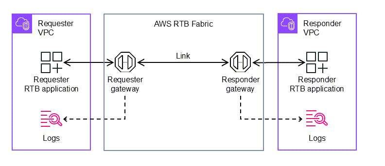
AWS RTB Fabric provides a dedicated, high-performance network environment for RTB workloads and partner integrations without requiring colocated, on-premises infrastructure or upfront commitments. The following diagram shows the high-level architecture of RTB Fabric.

AWS RTB Fabric also includes modules, a capability that helps customers bring their own and partner applications securely into the compute environment used for real-time bidding. Modules support containerized applications and foundation models (FMs) that can enhance transaction efficiency and bidding effectiveness. At launch, AWS RTB Fabric includes modules for optimizing traffic management, improving bid efficiency, and increasing bid response rates, all running inline within the service for consistent low-latency execution.

The growth of programmatic advertising has created a need for low-latency, cost-efficient infrastructure to support RTB workloads. AdTech companies process millions of bid requests per second across publishers, supply-side platforms (SSPs), and demand-side platforms (DSPs). These workloads are highly sensitive to latency because most RTB auctions must complete within 200–300 milliseconds and require reliable, high-speed exchange of OpenRTB requests and responses among multiple partners. Many companies have addressed this by deploying infrastructure in colocation data centers near key partners, which reduces latency but adds operational complexity, long provisioning cycles, and high costs. Others have turned to cloud infrastructure to gain elasticity and scale, but they often face complex provisioning, partner-specific connectivity, and long-term commitments to achieve cost efficiency. These gaps add operational overhead and limit agility. AWS RTB Fabric solves these challenges by providing a managed private network built for RTB workloads that delivers consistent performance, simplifies partner onboarding, and achieves predictable cost efficiency without the burden of maintaining colocation or custom networking setups.

Key capabilities
AWS RTB Fabric introduces a managed foundation for running RTB workloads at scale. The service provides the following key capabilities:

  • Simplified connectivity to AdTech partners – When you register an RTB Fabric gateway, the service automatically generates secure endpoints that can be shared with selected partners. Using the AWS RTB Fabric API, you can create optimized, private connections to exchange RTB traffic securely across different environments. External Links are also available to connect with partners who aren’t using RTB Fabric, such as those operating on premises or in third-party cloud environments. This approach shortens integration time and simplifies collaboration among AdTech participants.
  • Dedicated network for low-latency advertising transactions – AWS RTB Fabric provides a managed, high-performance network layer optimized for OpenRTB communication. It connects AdTech participants such as SSPs, DSPs, and publishers through private, high-speed links that deliver consistent single-digit millisecond latency. The service automatically optimizes routing paths to maintain predictable performance and reduce networking costs, without requiring manual peering or configuration.
  • Pricing model aligned with RTB economics – AWS RTB Fabric uses a transaction-based pricing model designed to align with programmatic advertising economics. Customers are billed per billion transactions, providing predictable infrastructure costs that align with how advertising exchanges, SSPs, and DSPs operate.
  • Built-in traffic management modules – AWS RTB Fabric includes configurable modules that help AdTech workloads operate efficiently and reliably. Modules such as Rate Limiter, OpenRTB Filter, and Error Masking help you control request volume, validate message formats, and manage response handling directly in the network path. These modules execute inline within the AWS RTB Fabric environment, maintaining network-speed performance without adding application-level latency. All configurations are managed through the AWS RTB Fabric API, so you can define and update rules programmatically as your workloads scale.

Getting started
Today, you can start building with AWS RTB Fabric using the AWS Management Console, AWS Command Line Interface (AWS CLI), or infrastructure-as-code (IaC) tools such as AWS CloudFormation and Terraform.

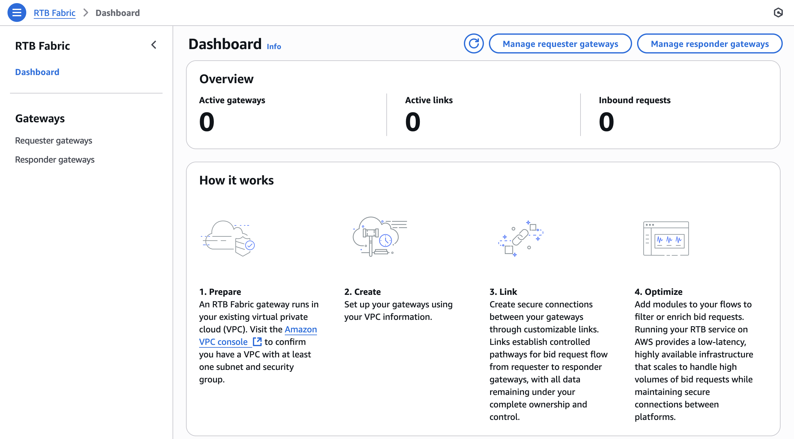
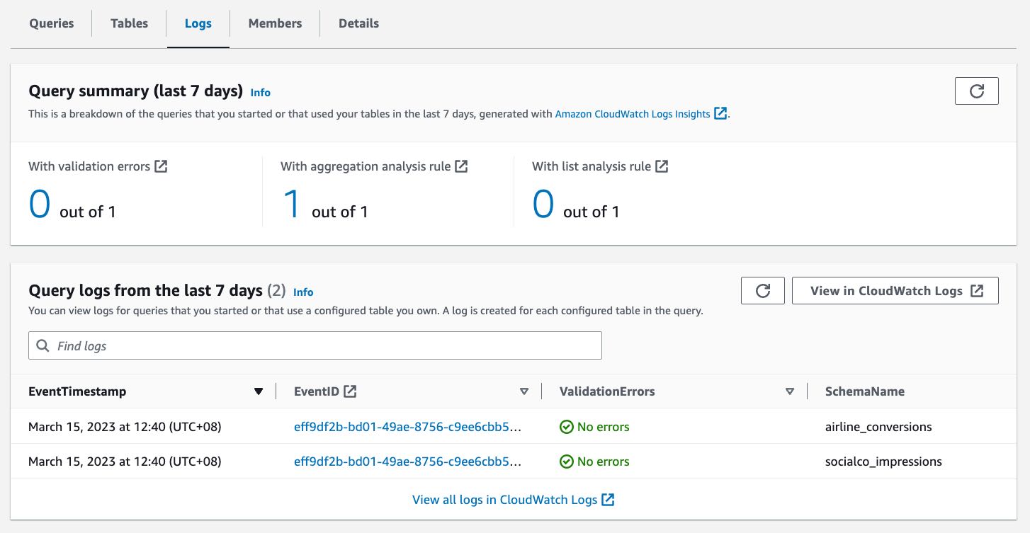
The console provides a visual entry point to view and manage RTB gateways and links, as shown on the Dashboard of the AWS RTB Fabric console.

You can also use the AWS CLI to configure gateways, create links, and manage traffic programmatically. When I started building with AWS RTB Fabric, I used the AWS CLI to configure everything from gateway creation to link setup and traffic monitoring. The setup ran inside my Amazon Virtual Private Cloud (Amazon VPC) endpoint while AWS managed the low-latency infrastructure that connected workloads.

To begin, I created a requester gateway to send bid requests and a responder gateway to receive and process bid responses. These gateways act as secure communication points within the AWS RTB Fabric.

# Create a requester gateway with required parameters
aws rtbfabric create-requester-gateway \
  --description "My RTB requester gateway" \
  --vpc-id vpc-12345678 \
  --subnet-ids subnet-abc12345 subnet-def67890 \
  --security-group-ids sg-12345678 \
  --client-token "unique-client-token-123"
# Create a responder gateway with required parameters
aws rtbfabric create-responder-gateway \
  --description "My RTB responder gateway" \
  --vpc-id vpc-01f345ad6524a6d7 \
  --subnet-ids subnet-abc12345 subnet-def67890 \
  --security-group-ids sg-12345678 \
  --dns-name responder.example.com \
  --port 443 \
  --protocol HTTPS

After both gateways were active, I created a link from the requester to the responder to establish a private, low-latency communication path for OpenRTB traffic. The link handled routing and load balancing automatically.

# Requester account creating a link from requester gateway to a responder gateway
aws rtbfabric create-link \
  --gateway-id rtb-gw-requester123 \
  --peer-gateway-id rtb-gw-responder456 \
  --log-settings '{"applicationLogs:{"sampling":"errorLog":10.0,"filterLog":10.0}}'
# Responder account accepting a link from requester gateway to responder gateway
aws rtbfabric accept-link \
  --gateway-id rtb-gw-responder456 \
  --link-id link-reqtoresplink789 \
  --log-settings '{"applicationLogs:{"sampling":"errorLog":10.0,"filterLog":10.0}}'

I also connected with external partners using External Links, which extended my RTB workloads to on-premises or third-party environments while maintaining the same latency and security characteristics.

# Create an inbound external link endpoint for an external partner to send bid requests to
aws rtbfabric create-inbound-external-link \
  --gateway-id rtb-gw-responder456
# Create an outbound external link for sending bid requests to an external partner
aws rtbfabric create-outbound-external-link \
  --gateway-id rtb-gw-requester123 \
  --public-endpoint "https://my-external-partner-responder.com"

To manage traffic efficiently, I added modules directly into the data path. The Rate Limiter module controlled request volume, and the OpenRTB Filter validated message formats inline at network speed.

# Attach a rate limiting module
aws rtbfabric update-link-module-flow \
  --gateway-id rtb-gw-responder456 \
  --link-id link-toresponder789 \
  --modules '{"name":"RateLimiter":"moduleParameters":{"rateLimiter":{"tps":10000}}}'

Finally, I used Amazon CloudWatch to monitor throughput, latency, and module performance, and I exported logs to Amazon Simple Storage Service (Amazon S3) for auditing and optimization.

All configurations can also be automated with AWS CloudFormation or Terraform, allowing consistent, repeatable deployment across multiple environments. With RTB Fabric, I could focus on optimizing bidding logic while AWS maintained predictable, single-digit millisecond performance across my AdTech partners.

For more details, refer to the AWS RTB Fabric User Guide.

Now available
AWS RTB Fabric is available today in the following AWS Regions: US East (N. Virginia), US West (Oregon), Asia Pacific (Singapore), Asia Pacific (Tokyo), Europe (Frankfurt), and Europe (Ireland).

AWS RTB Fabric is continually evolving to address the changing needs of the AdTech industry. The service expands its capabilities to support secure integration of advanced applications and AI-driven optimizations in real-time bidding workflows that help customers simplify operations and improve performance on AWS. To learn more about AWS RTB Fabric, visit the AWS RTB Fabric page.

Betty

Analyze media content using AWS AI services

Post Syndicated from Jack Bradham original https://aws.amazon.com/blogs/architecture/analyze-media-content-using-aws-ai-services/

Organizations managing large audio and video archives face significant challenges in extracting value from their media content. Consider a radio network with thousands of broadcast hours across multiple stations and the challenges they face to efficiently verify ad placements, identify interview segments, and analyze programming patterns.

In this post, we demonstrate how you can automatically transform unstructured media files into searchable, analyzable content. By combining Amazon Transcribe, Amazon Bedrock, Amazon QuickSight, and Amazon Q, organizations can achieve the following:

  • Process and transcribe media files upon upload
  • Identify commercials, interviews, and program segments
  • Extract insights using foundation models (FMs)
  • Create a searchable knowledge base
  • Generate rich visualizations for decision-making
  • Enable natural language queries across their media archive
  • Visualize complex information with intuitive graphics

In the following sections, we explore how these AWS services work together to help organizations unlock the full potential of their media content, whether for advertising compliance, content analysis, or discovering specific segments within thousands of hours of recordings.

Solution overview

This solution provides an event-driven media analysis pipeline that transforms how you manage and extract value from your content:

  • Streamline content management – Automatically process media files the moment they’re uploaded, saving time and reducing manual work
  • Unlock deeper insights – Generate accurate transcriptions that capture not just words, but the full context of your content—including speakers, timing, and key moments
  • Harness AI – Automatically extract meaningful insights and uncover hidden patterns in your media without extensive manual review
  • Build a searchable knowledge base – Turn scattered media files into a discoverable catalog that your entire team can use
  • Build a customizable interface – Create a customizable UI to search the catalog
  • Create powerful visualizations – Bring your insights to life with intuitive visualizations that make complex information immediately understandable

The following diagram illustrates our architecture.

Media Analysis Architecture

This event-driven architecture automatically processes and analyzes multimedia content using AWS services. The workflow consists of the following steps:

  1. A user uploads media files to an Amazon Simple Storage Service (Amazon S3) bucket. A “New Media” event triggers the first AWS Step Functions workflow. This workflow handles the initial cataloging based on values in the file name and launches the transcription process.
  2. Amazon Transcribe converts the audio into accurate, readable text. The transcribed content is securely saved to an S3 bucket for further analysis. A “Transcription Complete” event triggers the next step.
  3. A second Step Functions workflow processes the transcription. Using predefined prompts, Amazon Bedrock analyzes the transcripts to extract meaningful information. Key insights extracted from the transcript are stored in an S3 data lake.
  4. The processed results are organized systematically, structured by date (year/month/day) and tagged with relevant attributes. This organized data enables natural language queries through Amazon Q when used as a knowledge base, interactive visualizations using QuickSight, and straightforward content discovery and analysis.
  5. Amazon Athena serves as the data exploration tool to query the data lake. Athena is used as the data source in QuickSight, which turns complex data into clear, compelling visuals.

This architecture automatically transforms raw media content into searchable, analyzable data while maintaining an organized hierarchy for efficient access and analysis. The event-driven design provides automatic processing of new content as it arrives, and the combination of AWS AI services enables deep content understanding and insight extraction. Each AWS service plays a crucial role in transforming your media content:

  • Amazon Bedrock – Reviews content after transcription for insights and entity extraction:
    • Uses advanced FMs to analyze transcripts
    • Identifies commercials, interviews, and program segments
    • Extracts meaningful insights from content
  • Amazon EventBridge – Triggers actions in the cataloging workflow:
    • Monitors for new media files and completed transcriptions
    • Automatically triggers Step Functions workflows
  • AWS Lambda – Handles custom code actions needed in the workflow:
    • Facilitates interaction with Amazon Bedrock
    • Executes custom prompts on transcripts
    • Enables flexible, scalable processing
  • Amazon Q – Serves as the frontend and Retrieval Augmented Generation (RAG) engine:
    • Addresses enterprise generative AI needs by providing a turnkey solution with built-in security features like single sign-on (SSO) integration and responsible AI governance policies
    • Allows businesses to quickly deploy AI assistance while maintaining compliance, data privacy, and security standards
    • Enables natural language queries across the media archive
    • Links results to the source media files
    • Provides conversational access to content
  • Amazon QuickSight – Turns insights in beautiful visualization for better consumption:
    • Creates interactive dashboards and visualizations
    • Displays comprehensive media analytics
    • Helps track advertising, programming, and content patterns
  • Amazon S3 – Stores assets and the catalog:
    • Securely stores raw media files, transcripts, and processed data
    • Automatically triggers processing when new content is uploaded
  • AWS Step Functions – Orchestrates the entire content processing workflow:
    • Manages transcription and AI analysis steps
    • Provides robust error handling and automatic retries
  • Amazon Transcribe – Converts speech to accurate, readable text:
    • Identifies speakers and timestamps
    • Provides accurate transcriptions of audio content

Security considerations

Although this post focuses on the technical implementation of media content analysis, it’s important to acknowledge that production deployments should include comprehensive security measures:

  • Data storage security (Amazon S3):
    • Enable server-side encryption using AWS Key Management Service (AWS KMS) keys
    • Apply bucket policies restricting access to authorized principals only
    • Enable Amazon S3 Block Public Access at account and bucket levels
    • Enable versioning for data recovery
    • Implement lifecycle policies for data retention
    • Enable S3 access logging
    • Use presigned URLs for temporary access
  • Identity and Access Management (IAM):
    • Create dedicated service roles with minimum required permissions for:
      • Step Functions execution
      • Amazon Transcribe jobs
      • Amazon Bedrock API calls
      • Athena queries
    • Implement role-based access control
    • Regularly rotate credentials
    • Enable multi-factor authentication (MFA) for all users
    • Use AWS Organizations for multi-account management
  • Network security:
    • Deploy virtual private cloud (VPC) endpoints for:
      • Amazon S3
      • Athena
      • QuickSight
    • Implement network access control lists (ACLs) and security groups
    • Enable VPC Flow Logs
    • Use AWS PrivateLink where applicable
    • Configure route tables to control traffic flow
  • Data encryption:
    • Implement AWS KMS encryption for S3 objects
    • Use TLS 1.2+ for all API communications
    • Enable automatic key rotation in AWS KMS
    • Implement envelope encryption for sensitive data
  • Monitoring and detection:
    • Enable AWS CloudTrail for API activity logging
    • Configure Amazon GuardDuty for threat detection
    • Set up Amazon CloudWatch:
      • Metrics for service health
      • Alarms for security events
      • Log groups for application logs
    • Enable S3 server access logging
    • Configure VPC Flow Logs
  • Access controls:
    • Implement fine-grained access controls for:
      • Amazon Bedrock model access
      • Athena query permissions
      • QuickSight dashboard sharing
    • Conduct regular access reviews

Additionally, compliance requirements and data governance policies might impact how you implement this solution in your environment.

These security considerations are crucial but beyond the scope of this post. We recommend consulting AWS security best practices and working with your security team to implement appropriate measures for your specific use case. For more information on AWS security best practices, refer to Best Practices for Security, Identity, & Compliance.

The following sections walk you through setting up each component of the architecture to help you transform raw media into actionable insights.

Prerequisites

The following are the prerequisites to follow along this post:

Create S3 buckets

For this solution, we create three distinct buckets to support the media analytics workflow:

  • Raw media bucket for incoming files
  • Transcription outputs bucket
  • Processed insights bucket

For instructions on creating buckets, refer to Creating a general purpose bucket.

Configure EventBridge

You can enable event notifications on the raw media bucket to trigger your automated workflow through EventBridge. Establish your automation backbone by monitoring S3 bucket activities. When new media arrives or transcription completes, EventBridge will trigger the appropriate workflow, providing continuous processing. For further instructions, refer to Creating rules that react to events in Amazon EventBridge.

The following are two example triggers that can be used to filter events and trigger Step Functions workflows. The following is an example filter for new media files:

{
  "source": ["aws.s3"],
  "detail-type": ["Object Created"],
  "detail": {
    "bucket": {
      "name": ["rawinputbucket"]
    }
  }
}

The following is an example filter for new transcripts added to the data lake:

{
  "source": ["aws.s3"],
  "detail-type": ["Object Created"],
  "detail": {
    "bucket": {
      "name": ["business-data-lake"]
    },
    "object": {
      "key": [{
        "suffix": ".transcription"
      }]
    }
  }
}

Create Step Functions workflows

We design the orchestration layer with two key workflows. The first handles media intake and transcription, and the second manages AI analysis. Each workflow includes safeguards for potential failures and retry mechanisms. For further instructions, refer to Learn how to get started with Step Functions.

The following diagram shows an example of processing new media uploads for indexing and transcription.

Media Analysis - Step Function Example

The following diagram shows an example of the Step Functions workflow that analyzes the transcription.

Set up Amazon Transcribe

To create an Amazon Transcribe job, you need permissions to do so. You can implement a speech-to-text conversion with powerful features like language detection, speaker identification, and custom vocabulary support to provide accurate transcription of your media content. For further instructions, refer to How Amazon Transcribe works.

Configure Amazon Bedrock

You can power your AI analysis engine by setting up precise prompts that extract meaningful insights. Amazon Bedrock processes transcripts to identify key segments, speakers, and topics, transforming raw text into structured data. For instructions, refer to Design a prompt.

The following is a sample prompt:

You will be reviewing a radio transcription to identify advertisements and extract relevant details. Your task is to analyze the provided transcript and output the results in a specific JSON format based on a given schema.
Please follow these steps to complete the task:
1. Carefully read through the entire transcript.
2. Identify all advertisements within the transcript. Look for clear indicators such as product mentions, promotional language, or transitions from regular content to commercial content.
3. For each advertisement you identify, determine the following information:
    - Company: The name of the company being advertised
    - Start time: The timestamp in the transcript where the ad begins
    - End time: The timestamp in the transcript where the ad ends
    - Product: The specific product or service being advertised
4. Format your findings into a JSON object that follows the provided schema. Each advertisement should be a separate object within an array.
5. Ensure these fields in your response are provided for each advertisement.. All are required fields: company, starttime, endtime, product. 
6. Use precise timestamps for start and end times. If exact times are not available, make a best estimate based on the transcript's context.
7. If a particular field is unclear or not explicitly mentioned in the transcript, you may use "Unknown" as the value.
8. Only respond with json and nothing else. Do not provide comments or explain your answer. 
9. Surround the JSON response with standard ```json markers
Here's an example of how your output should be formatted:
{
"advertisements": [
        {
            "company": "TechGadgets Inc.",
            "starttime": "00:05:30",
            "endtime": "00:06:15",
            "product": "SmartHome Hub"
        },
        {
            "company": "FreshFoods Market",
            "starttime": "00:15:45",
            "endtime": "00:16:30",
            "product": "Organic Produce Delivery Service"
        }
    ]
}
Do not add any fields that are not specified in the schema, and ensure all required fields are present for each advertisement.

Create a structured data lake

We create a hierarchical data organization strategy that enables efficient access and analysis. You can use AWS Glue crawlers to automatically discover and catalog your media metadata. For instructions, refer to Using crawlers to populate the Data Catalog. Configure Athena tables to enable SQL-based querying of your media insights:

CREATE OR REPLACE VIEW "commercials_view" AS 
SELECT
  metadata.market market
, metadata.station_call station_call
, metadata.format_type format_type
, CAST(metadata.timestamp AS timestamp) timestamp
, ads.company adCompany
, ads.product adProduct
, ads.starttime
, ads.endtime
FROM
  (commercials
CROSS JOIN UNNEST(advertisements) t (ads))

Set Up Amazon Q

You can enable natural language interaction with your media archive using Amazon Q Business. Configure the knowledge base and metadata to make your content searchable and accessible through conversational queries. Use the processed insights S3 buckets to configure the knowledge base. For instructions, refer to Getting started with Amazon Q Business.

The following screenshot shows example conversations with an AI assistant.

Build QuickSight dashboards

With QuickSight, you can create visual analytics that bring your data to life. Connect to Athena views to display advertising patterns, content analysis, and performance metrics in interactive dashboards. For more information, refer to Tutorial: Create an Amazon QuickSight dashboard.

The following screenshots are a few examples of dashboards created for a fictitious radio station as part of our use case.

Validate and optimize your media analytics solution

After you implement your media analytics architecture, follow these critical steps to achieve robust performance and alignment with your organization’s needs. First, configure a comprehensive testing approach. Imagine you’re preparing to launch your media analysis solution. Your testing journey begins with accuracy validation:

  • Compare transcription outputs against original media
  • Verify AI-generated insights for precision
  • Use representative sample sets from your content library

You start by taking a recently processed radio show and comparing its transcription against the original broadcast. Your team meticulously reviews the AI-generated insights, checking if key moments like ad transitions or interview segments are correctly identified. To make sure your system works across all content types, you select diverse samples from your library—perhaps a morning talk show, an evening news segment, and a weekend sports broadcast. Next, you delve into performance benchmarking:

  • Measure processing time for different media types
  • Evaluate resource utilization across AWS services
  • Identify potential bottlenecks in the workflow

Time how long it takes to process different types of media files, from short commercial segments to lengthy program recordings. As you watch how your AWS services respond under various loads, you can monitor resource consumption patterns. This helps you identify processing bottlenecks—for instance, you might discover that certain file types take longer to transcribe or that concurrent processing needs optimization. Finally, you put yourself in your users’ shoes for a thorough user experience assessment:

  • Test natural language queries with Amazon Q
  • Validate search result relevance
  • Gather feedback from potential end-users

Team members can interact with Amazon Q, asking questions they would naturally pose when searching for specific content. For example, you can test whether searching for “interviews about climate change last week” returns relevant results. Gathering feedback from potential users—perhaps a content manager with different needs than a compliance officer—provides invaluable insights. Their real-world experiences guide your refinements and make sure the system serves its intended purpose. This comprehensive testing approach, combining structured evaluation with real-world scenarios, sets the stage for a robust and user-friendly media analysis solution. As your media analysis solution moves from initial deployment to production, optimizing its performance becomes crucial for both cost-efficiency and user satisfaction. A radio network processing thousands of hours of content weekly might find that even small improvements in transcription accuracy or processing speed can lead to significant cost savings and better content discoverability. Similarly, a marketing team analyzing ad placements across multiple stations needs precise insights to make data-driven decisions about advertising effectiveness. With these business imperatives in mind, consider the following configuration optimization strategies:

  • Transcription refinement:
    • Adjust language models for domain-specific terminology
    • Fine-tune speaker identification settings
    • Implement custom vocabularies for improved accuracy
  • AI insight generation:
    • Refine prompts for more targeted analysis
    • Experiment with different AI models
    • Align extraction parameters with business objectives
  • Scalability considerations:
    • Test workflow performance with increasing media volumes
    • Implement appropriate auto scaling configurations
    • Monitor cost-effectiveness of your architecture
  • Continuous improvement:
    • Establish regular review cycles
    • Track key performance metrics
    • Iterate on your solution based on real-world usage

We recommend starting with a pilot implementation and gradually expanding your media analytics capabilities.

Clean up

To avoid incurring ongoing charges, clean up the resources you created as part of this solution:

  1. Delete QuickSight resources:
    1. Delete dashboards created for media analytics.
    2. Delete the datasets connected to Athena.
    3. If no longer needed, delete the QuickSight Enterprise subscription.
  2. Delete S3 buckets:
    1. Empty and delete the raw media bucket, transcription outputs bucket, and processed insights bucket.
  3. Remove EventBridge rules:
    1. Delete the rules created for monitoring S3 bucket activities.
    2. Remove targets associated with these rules.
  4. Delete Step Functions workflows:
    1. Delete the media intake and transcription workflow.
    2. Delete the AI analysis workflow.
  5. Remove Lambda functions:
    1. Delete Lambda functions created for interaction with Amazon Bedrock.
    2. Remove associated IAM roles and policies.
  6. Clean up data lake components:
    1. Delete Athena views and tables.
    2. Remove AWS Glue crawlers and databases.
    3. Delete stored query results.
  7. Remove Amazon Q configurations:
    1. Delete knowledge bases created.
    2. Remove custom configurations.
  8. Remove Amazon Bedrock settings:
    1. Remove custom prompts.
    2. Disable access to FMs if no longer needed.
  9. Delete Amazon Transcribe settings:
    1. Remove custom vocabularies.
    2. Delete stored transcription jobs.
  10. Remove IAM resources:
    1. Delete custom IAM roles created for this solution.
    2. Remove associated IAM policies.
  11. Complete additional cleanup:
    1. Delete CloudWatch Logs groups associated with Lambda functions.
    2. Remove CloudWatch alarms or metrics created for monitoring.
    3. Delete saved queries in Athena.

Common use cases

Organizations in different sectors can use this architecture to unlock value from their audio and video content. You can adapt this solution to meet your specific needs, such as managing broadcast media, corporate communications, educational materials, and more. Let’s explore how different industries might apply this technology:

  • Media and broadcasting:
    • Track advertising compliance
    • Verify media placement accuracy
    • Analyze broadcast content at scale
  • Corporate and enterprise:
    • Convert meeting recordings into searchable knowledge bases
    • Identify key decisions and action items
    • Enhance organizational knowledge management
  • Education and training:
    • Create comprehensive, topic-based course catalogs
    • Index training materials for quick retrieval
    • Support continuous learning initiatives
  • Legal services:
    • Generate precise, timestamped transcripts
    • Develop searchable legal proceeding archives
    • Improve document review efficiency
  • Healthcare:
    • Extract critical medical insights from consultations
    • Categorize patient interaction data
    • Support clinical documentation processes
  • Government and public sector:
    • Build comprehensive public meeting archives
    • Implement automated topic categorization
    • Enhance transparency and accessibility
  • Customer service:
    • Analyze call recordings for quality improvement
    • Identify service trends and customer pain points
    • Drive continuous customer experience enhancement

This media analytics architecture demonstrates notable versatility. By using AI, organizations can transform raw audio and video content into structured, meaningful insights that drive decision-making across industries.

Conclusion

In this post, we demonstrated how to use AWS services to convert unstructured media content into actionable intelligence. By combining Amazon Transcribe, Amazon Bedrock, QuickSight, and Amazon Q, you can create a scalable, automated solution for media analysis that adapts to your organizational needs.

This solution offers the following key architectural advantages:

  • Automated media file processing at scale
  • AI-powered insight generation
  • Natural language search capabilities
  • Interactive decision-making visualizations
  • Flexible, maintainable infrastructure

Organizations can now convert content into searchable knowledge, extract insights automatically, develop data-driven content strategies, and enhance operational efficiency through automation.

As audio and video content generation continues to accelerate, the ability to efficiently process and extract value becomes increasingly critical. This architecture provides a robust foundation for current needs while remaining adaptable to future technological innovations.

We invite you to explore how this media analytics solution can address your organization’s unique challenges. Consider your specific use cases and unlock the insights waiting to be discovered in your media archives.


About the authors

How SmugMug Increased Data Modeling Productivity with Amazon Q Developer

Post Syndicated from Will Matos original https://aws.amazon.com/blogs/devops/how-smugmug-increased-data-modeling-productivity-with-amazon-q-developer/

This post is co-written with Dr. Geoff Ryder, Manager, at SmugMug.

Introduction

SmugMug operates two very large online photo platforms: SmugMug and Flickr. These platforms enable more than 100 million customers to safely store, search, share, and sell tens of billions of photos every day. However, the data science and engineering team at SmugMug and Flickr often faces complex data modeling challenges that require significant time to resolve.

These challenges arise due to several factors. First, the team has to contend with diverse datasets from different sources. Additionally, the database schema and tables are highly complex, and the team needs to quickly understand application (PHP) code and database table structures in order to generate the necessary complex database queries. Specifically, SmugMug uses Amazon Redshift as its cloud data warehouse to analyze patterns in petabyte-scale data stored in Amazon S3, as well as transactional data in Amazon Aurora and Amazon DynamoDB. This allows them to generate dozens of business reports daily.

However, the complexity increases further as many database tables also need to be imported from third-party organizations into Amazon Redshift, where they are joined with SmugMug and Flickr’s internal tables. In extreme cases, properly modeling all these database tables and handling issues like granularity, cardinality, timestamps and missing data could take years – an impractical timeline for the business. We are excited to walk through SmugMug’s data modeling use cases and how SmugMug uses Amazon Q Developer to improve the data science and engineering team’s productivity.

Discovering Amazon Q Developer

SmugMug was one of the first customers to pilot Amazon Q Developer (previously Amazon CodeWhisperer), the most capable AI-powered assistant for software development that re-imagines the experience across the entire software development lifecycle, making it easier and faster to build, secure, manage, optimize, operate, and transform applications on AWS. There are multiple Amazon Q Developer use cases at SmugMug and Flickr, such as using Amazon Q Developer agent (/dev) for software development (i.e. generating implementation plans and the accompanying code), generating inline code suggestions, asking Amazon Q Developer in chat about AWS services and best practices, and analyzing AWS usage and costs for Cloud Financial Management (CFM) needs. For the data science and engineering team specifically, the key feature is chatting with Amazon Q Developer in integrated development environments (IDEs) like Intellij DataGrip. The data analysts and data scientists at SmugMug and Flickr ask questions in Amazon Q Developer chat to analyze database schemas, generate data model diagrams from DDL (Data Definition Language) statements, convert queries between languages, automatically generate complex database queries for data analysis, generate code to validate table contents, and predict trends using ML (Machine Learning).

Implementing Amazon Q Developer

To solve the data modeling challenges SmugMug faced, the team collaborated closely with their AWS Account Team, AWS Professional Services, and the Amazon Q Developer service team to create and test a data modeling assistant solution using Amazon Q Developer.

As a first step, the data modeler needs to bring the right metadata to bear. For simpler cases, the commands “show view myschema.v” or “show table myschema.t“ retrieve DDL schema information about the specified view or table from Amazon Redshift into the IDE console.

Here’s an example using simulated data for a hypothetical company. For this typical company that handles orders for products, the result of typing “show table sample.orderinfo” and “show table sample.skuinfo”might be:

Image of SQL statement generated by the show table statement. "CREATE TABLE sample.skuinfo ( sku_id bigint ENCODE raw, sku_vendor bigint ENCODE az64, sku_category character varying(18) ENCODE lzo, sku_description character varying(255) ENCODE lzo, date_sku_created timestamp without time zone ENCODE az64, date_sku_updated timestamp without time zone ENCODE az64, pipeline_inserted_at timestamp without time zone ENCODE az64 ) DISTSTYLE KEY SORTKEY ( sku_id );"

Image of SQL statement generated by the show table statement. "CREATE TABLE sample.orderinfo ( order_id bigint ENCODE raw, shipper_id bigint ENCODE az64 distkey, product_id bigint ENCODE az64, quantity_ordered integer ENCODE az64, date_order_placed timestamp without time zone ENCODE az64 ) DISTSTYLE KEY SORTKEY ( order_id );"

This DDL text is now in the open tab. By selecting the text to highlight it, that DDL text becomes part of the context that Amazon Q Developer sees. The modeler can start asking questions about them in the Amazon Q Developer chat window in the IDE.

Diagram showing what is considered part of the context included in a request including the RAG query result, related documents when using the at-workspace key word, the highlighted text in the IDE open tab,the chat history, and the prompt.

In complex scenarios, establishing the correct modeling context requires a combination of schema information, legacy SQL, application source code in various programming languages, sample values, and natural language documentation. Amazon Q Developer addresses this by creating a local index of relevant files and content. When a question is asked using @workspace, this index is consulted to identify and include pertinent sections of code and information in the request. (See this article for additional details on workspace). The prompt plays a crucial role in measuring similarity, so providing comprehensive context within it is essential. To optimize this process, the IDE settings feature a tunable workspace index function, allowing for enhanced performance in identifying and incorporating relevant context.

Image showing the Amazon Q Settings window where you enable the Workspace feature by checking the "Workspace index" box. You can also change the number of worker threads used, and the maximum workspace index size in MB.

Workspace Index Settings

By adopting Amazon Q Developer as a team, we are able to jointly develop and share proprietary prompt text to address the four steps in our modeling process, as follows.

Step 1. Define the goal for the data modeling project

From prior knowledge, sketch a high-level goal for a data model. Gather the data for it manually, or by e.g. querying a vector database and adding its documents to the project.

For this example, we choose as the goal to compute aggregated metrics from a new table or view composed of two existing tables, sample.orderinfo and sample.skuinfo. These contain simulated data about product sales that are common to many companies. The order table is in the style of a fact table that logs customer orders, and the stock keeping unit (SKU) table is a dimension table that provides additional data points of interest about each order. The order and SKU information need to be combined by a join operation before we can compute the metrics. We would like Amazon Q Developer to tell us how to write that SQL join statement.

Step 2. Conduct an exploratory analysis and generate candidates

Next, prompt Amazon Q Developer for candidate foreign keys to join the tables, and for SQL code to execute those joins. Generate an entity-relationship diagram (ERD) as a visual aid. Prompts do not have to be complicated. For example:

@workspace What columns of database tables sample.orderinfo and sample.skuinfo 
would be best to join the two tables? Provide SQL code for the join. Draw an 
entity relationship diagram that shows the joins between the two tables, and 
includes only the fields involved in the join. Add a crow's foot cardinality 
marker to indicate a 1:many relationship, and add it next to the high 
cardinality table.

Image with the first part of the response to the prompt with the following text: "Based on the table schemas, sku_id is the appropriate column to join these tables. The relationship is likely one-to-many (1:M) where one SKU can appear in multiple orders. Here's the SQL join: SELECT o.order_id, o.sku_id, s.sku_description FROM sample.orderinfo o JOIN sample.skuinfo s ON o.sku_id = s.sku_id;

Image with the second part of the response to the prompt with the ASCII relationship diagram showing the join relationship.

Each time tables are joined together, new aggregated metrics become available to drive business insights. Now, for instance, we can find the top selling SKUs in October thanks to our results:

Image shows the top 5 results from the prior query showing the top skus in October.

Sometimes we need to look at code written in languages other than SQL to complete the data model. For example, the names of some vendors this company works with happen to appear in application PHP code as human readable strings, but are saved in the application database as numbers. The analytics data staged in Redshift only contain the numbers. So, we pull a copy of the PHP text file into @workspace, and ask Amazon Q Developer to translate the relevant string-integer mappings into a SQL case statement.

Image shows the selected PHP code with a switch statement mapping Vendor Ids to Vendor Names.

PHP Switch statement showing the mapping of Vendor Ids to String Names.

I am a Redshift database administrator and I am working on a data modeling 
problem. I would like to write SQL statements to join tables sample.orderinfo 
and sample.skuinfo. Please write that SQL to join the two tables. Also, I 
would like to write a SQL case statement to recover all string values defined 
in PHP that are represented as integer values in the database table.

The output of that prompt is shown below.

Image showing the updated SQL query that maps the Vendor Id to the Vendor Name.

Amazon Q Developer automatically detected the PHP switch case statement, converted to SQL, and added it to the final query. Many other programming languages are supported, and modelers should try this technique with other kinds of source code. Note that data scientists and analysts may not know where to look in complex application code for these details, so this discovery-plus-code translation step is a net new benefit to our company that is only possible thanks to Amazon Q Developer.

Step 3. Create code to test the analysis

Now we request SQL source code for a battery of small test queries. These can return cardinality, grain, arithmetic, and null count results.

Please write a short SQL test to compute counts of the key fields that are used 
in the joins, which will verify the cardinality assignments indicated in the 
entity relationship diagram above. The SQL test should compare distinct counts 
to total counts and null counts when it verifies the cardinality.

Image of resulting SQL queries to check cardinality.

Step 4. Validate the results of the analysis

Run the test queries to see if the candidate solution from step 2 meets our goals. The “Insert at cursor” button at the bottom of the response is handy for this. The data modeler can easily spot an error in the join logic and ERD from inspecting the output of the test query. (Or, if it’s hard to interpret the results, keep making the test queries simpler.) If errors arise from the AI misinterpreting or miscalculating a result, or from a vaguely worded prompt, simply adjust the prompt in step 2 to fix the known errors, and repeat steps 2 – 4.

Image showing the query results from the cardinality query.

After a few iterations, taking from seconds to at most tens of minutes each, the modeling errors have been worked out and we arrive at a valid production query.

Key Benefits and Results

With this Amazon Q Developer powered solution and iterative approach, SmugMug has achieved highly accurate data modeling results across numerous database tables. Once the correct modeling configuration is established, various useful outputs may become available.

We already described production SQL, unit tests, and ERDs for documentation. By the end of the process, because Amazon Q Developer has a good understanding of the data it just modeled in its chat history, it will also generate useful Python machine learning programs to predict business trends. Here is a prompt for that, and a partial screenshot of the Python output:

Please write Python code to implement a linear regression that predicts the 
quantity_ordered value based on other fields in the data set. Choose predictor 
variables that are less likely to cause multi-collinearity problems.

Image showing the python code generated to predict quantity_ordered value.

This only shows the model training step, but the full response included all library imports, a Redshift query, feature engineering steps, ML performance metrics, and code for plotting the metrics. And the AI can produce other types of predictive models. For example, you can try:

Please write Python code to implement an XGBoost model that predicts the 
quantity_ordered value based on other fields in the data set.

Ultimately, the solution has improved team productivity for both existing and new team members, while maintaining legacy knowledge needed to onboard new team members more efficiently. Key benefits include:

  1. Reducing SmugMug data analyst and scientist’s time spent on data modeling tasks from days to hours, allowing them to reallocate this time to other high-priority projects.
  2. Automating the generation of BI documentation and predictive ML, also saving crucial time.
  3. Providing net new value by translating application code constant definitions into SQL. Due to organizational boundaries, we would not have achieved this without an assist from the AI.

Future Plans and Expansion

SmugMug conducted the initial data modeling use case testing with over a dozen data science team members and analysts. We are moving on to analyze more complex tables and data schemas, and generating Python code in Amazon SageMaker for ML tasks like data preparation, training, inference, and MLOps. From our experience, Amazon Q Developer has become a preferred internal tool for development that has a data modeling component, and its use continues to expand to different groups around the company.

For SmugMug’s data modeling projects, we continue to enhance the four-step process described above. In order to gather the most relevant context to solve a problem, we build vector database collections to pull from schemas, older SQL code, application source code, BI tool content, and curated documentation. The vector search operation surfaces the right content, and spares data modelers from manually searching in different code archives. We use ChromaDB to do the searches, and bring the results from ChromaDB into the workspace as additional files.

Conclusion

Using Amazon Q Developer for data modeling use cases, SmugMug has managed to increase data science and engineering team productivity by up to 100% when compared to prior workflows. To explore how Amazon Q Developer can benefit your organization, get started here. If you have questions or suggestions, please leave a comment below.

About the Authors

Image of Dr. Geoffrey Ryder

Dr. Geoffrey Ryder

Dr. Geoff Ryder serves as the Manager of Data Science and Engineering at SmugMug, where he leads Team Prophecy in managing the company’s cloud-based data warehouse and analytics platforms. With a focus on leveraging the best AI tools, his team empowers photography clients to enhance their sales of both physical and digital photographic products. Geoff brings over two decades of experience in technical and business roles across Silicon Valley companies, and holds a PhD in Computer Engineering from UC-Santa Cruz.

Will Matos

Will Matos is a Principal Specialist Solutions Architect at AWS, revolutionizing developer productivity through Generative AI, AI-powered chat interfaces, and code generation. With 25 years of tech experience, and over 9 years with AWS, he collaborates with product teams to create intelligent solutions that streamline workflows and accelerate software development cycles. A thought leader engaging early adopters, Will bridges innovation and real-world needs.

Sreenivas Adiki

Sreenivas Adiki is a Sr. Customer Delivery Architect in ProServe, with a focus on data and analytics. He ensures success in designing, building, optimizing, and transforming in the area of Big Data/Analytics. Ensuring solutions are well-designed for successful deployment, Sreenivas participates in deep architectural discussions and design exercises. He has also published several AWS assets, such as whitepapers and proof-of-concept papers.

Kevin Bell

Kevin Bell is a Sr. Solutions Architect at AWS based in Seattle. He has been building things in the cloud for about 10 years. You can find him online as @bellkev on GitHub.

Corey Keane

Corey Keane is a Media and Entertainment (M&E) Sr. Account Manager at AWS. Corey has held a number of positions at Amazon and AWS throughout his 8 years with the company across M&E—including technical business development for strategic partnerships with international game developers, in addition to his current role managing AWS customers in the Media vertical. He leans on his pan-Amazon experience from working on other teams to identify new partnerships between our customers and other Amazon businesses to bring disruptive products to market.

AWS Clean Rooms Differential Privacy enhances privacy protection of your users data (preview)

Post Syndicated from Donnie Prakoso original https://aws.amazon.com/blogs/aws/aws-clean-rooms-differential-privacy-enhances-privacy-protection-of-your-users-data-preview/

Starting today, you can use AWS Clean Rooms Differential Privacy (preview) to help protect the privacy of your users with mathematically backed and intuitive controls in a few steps. As a fully managed capability of AWS Clean Rooms, no prior differential privacy experience is needed to help you prevent the reidentification of your users.

AWS Clean Rooms Differential Privacy obfuscates the contribution of any individual’s data in generating aggregate insights in collaborations so that you can run a broad range of SQL queries to generate insights about advertising campaigns, investment decisions, clinical research, and more.

Quick overview on differential privacy
Differential privacy is not new. It is a strong, mathematical definition of privacy compatible with statistical and machine learning based analysis, and has been used by the United States Census Bureau as well as companies with vast amounts of data.

Differential privacy helps with a wide variety of use cases involving large datasets, where adding or removing a few individuals has a small impact on the overall result, such as population analyses using count queries, histograms, benchmarking, A/B testing, and machine learning.

The following illustration shows how differential privacy works when it is applied to SQL queries.

When an analyst runs a query, differential privacy adds a carefully calibrated amount of error (also referred to as noise) to query results at run-time, masking the contribution of individuals while still keeping the query results accurate enough to provide meaningful insights. The noise is carefully fine-tuned to mask the presence or absence of any possible individual in the dataset.

Differential privacy also has another component called privacy budget. The privacy budget is a finite resource consumed each time a query is run and thus controls the number of queries that can be run on your datasets, helping ensure that the noise cannot be averaged out to reveal any private information about an individual. When the privacy budget is fully exhausted, no more queries can be run on your tables until it is increased or refreshed.

However, differential privacy is not easy to implement because this technique requires an in-depth understanding of mathematically rigorous formulas and theories to apply it effectively. Configuring differential privacy is also a complex task because customers need to calculate the right level of noise in order to preserve the privacy of their users without negatively impacting the utility of query results.

Customers also want to enable their partners to conduct a wide variety of analyses including highly complex and customized queries on their data. This requirement is hard to support with differential privacy because of the intricate nature of the calculations involved in calibrating the noise while processing various query components such as aggregations, joins, and transformations.

We created AWS Clean Rooms Differential Privacy to help you protect the privacy of your users with mathematically backed controls in a few clicks.

How differential privacy works in AWS Clean Rooms
While differential privacy is quite a sophisticated technique, AWS Clean Rooms Differential Privacy makes it easy for you to apply it and protect the privacy of your users with mathematically backed, flexible, and intuitive controls. You can begin using it with just a few steps after starting or joining an AWS Clean Rooms collaboration as a member with abilities to contribute data.

You create a configured table, which is a reference to your table in the AWS Glue Data Catalog, and choose to turn on differential privacy while adding a custom analysis rule to the configured table.

Next, you associate the configured table to your AWS Clean Rooms collaboration and configure a differential privacy policy in the collaboration to make your table available for querying. You can use a default policy to quickly complete the setup or customize it to meet your specific requirements. As part of this step, you will configure the following:

Privacy budget
Quantified as a value that we call epsilon, the privacy budget controls the level of privacy protection. It is a common, finite resource that is applied for all of your tables protected with differential privacy in the collaboration because the goal is to preserve the privacy of your users whose information can be present in multiple tables. The privacy budget is consumed every time a query is run on your tables. You have the flexibility to increase the privacy budget value any time during the collaboration and automatically refresh it each calendar month.

Noise added per query
Measured in terms of the number of users whose contributions you want to obscure, this input parameter governs the rate at which the privacy budget is depleted.

In general, you need to balance your privacy needs against the number of queries you want to permit and the accuracy of those queries. AWS Clean Rooms makes it easy for you to complete this step by helping you understand the resulting utility you are providing to your collaboration partner. You can also use the interactive examples to understand how your chosen settings would impact the results for different types of SQL queries.

Now that you have successfully enabled differential privacy protection for your data, let’s see AWS Clean Rooms Differential Privacy in action. For this demo, let’s assume I am your partner in the AWS Clean Rooms collaboration.

Here, I’m running a query to count the number of overlapping customers and the result shows there are 3,227,643 values for tv.customer_id.

Now, if I run the same query again after removing records about an individual from coffee_customers table, it shows a different result, 3,227,604 tv.customer_id. This variability in the query results prevents me from identifying the individuals from observing the difference in query results.

I can also see the impact of differential privacy, including the remaining queries I can run.

Available for preview
Join this preview and start protecting the privacy of your users with AWS Clean Rooms Differential Privacy. During this preview period, you can use AWS Clean Rooms Differential Privacy wherever AWS Clean Rooms is available. To learn more on how to get started, visit the AWS Clean Rooms Differential Privacy page.

Happy collaborating!
Donnie

AWS Clean Rooms ML helps customers and partners apply ML models without sharing raw data (preview)

Post Syndicated from Donnie Prakoso original https://aws.amazon.com/blogs/aws/aws-clean-rooms-ml-helps-customers-and-partners-apply-ml-models-without-sharing-raw-data-preview/

Today, we’re introducing AWS Clean Rooms ML (preview), a new capability of AWS Clean Rooms that helps you and your partners apply machine learning (ML) models on your collective data without copying or sharing raw data with each other. With this new capability, you can generate predictive insights using ML models while continuing to protect your sensitive data.

During this preview, AWS Clean Rooms ML introduces its first model specialized to help companies create lookalike segments for marketing use cases. With AWS Clean Rooms ML lookalike, you can train your own custom model, and you can invite partners to bring a small sample of their records to collaborate and generate an expanded set of similar records while protecting everyone’s underlying data.

In the coming months, AWS Clean Rooms ML will release a healthcare model. This will be the first of many models that AWS Clean Rooms ML will support next year.

AWS Clean Rooms ML helps you to unlock various opportunities for you to generate insights. For example:

  • Airlines can take signals about loyal customers, collaborate with online booking services, and offer promotions to users with similar characteristics.
  • Auto lenders and car insurers can identify prospective auto insurance customers who share characteristics with a set of existing lease owners.
  • Brands and publishers can model lookalike segments of in-market customers and deliver highly relevant advertising experiences.
  • Research institutions and hospital networks can find candidates similar to existing clinical trial participants to accelerate clinical studies (coming soon).

AWS Clean Rooms ML lookalike modeling helps you apply an AWS managed, ready-to-use model that is trained in each collaboration to generate lookalike datasets in a few clicks, saving months of development work to build, train, tune, and deploy your own model.

How to use AWS Clean Rooms ML to generate predictive insights
Today I will show you how to use lookalike modeling in AWS Clean Rooms ML and assume you have already set up a data collaboration with your partner. If you want to learn how to do that, check out the AWS Clean Rooms Now Generally Available — Collaborate with Your Partners without Sharing Raw Data post.

With your collective data in the AWS Clean Rooms collaboration, you can work with your partners to apply ML lookalike modeling to generate a lookalike segment. It works by taking a small sample of representative records from your data, creating a machine learning (ML) model, then applying the particular model to identify an expanded set of similar records from your business partner’s data.

The following screenshot shows the overall workflow for using AWS Clean Rooms ML.

By using AWS Clean Rooms ML, you don’t need to build complex and time-consuming ML models on your own. AWS Clean Rooms ML trains a custom, private ML model, which saves months of your time while still protecting your data.

Eliminating the need to share data
As ML models are natively built within the service, AWS Clean Rooms ML helps you protect your dataset and customer’s information because you don’t need to share your data to build your ML model.

You can specify the training dataset using the AWS Glue Data Catalog table, which contains user-item interactions.

Under Additional columns to train, you can define numerical and categorical data. This is useful if you need to add more features to your dataset, such as the number of seconds spent watching a video, the topic of an article, or the product category of an e-commerce item.

Applying custom-trained AWS-built models
Once you have defined your training dataset, you can now create a lookalike model. A lookalike model is a machine learning model used to find similar profiles in your partner’s dataset without either party having to share their underlying data with each other.

When creating a lookalike model, you need to specify the training dataset. From a single training dataset, you can create many lookalike models. You also have the flexibility to define the date window in your training dataset using Relative range or Absolute range. This is useful when you have data that is constantly updated within AWS Glue, such as articles read by users.

Easy-to-tune ML models
After you create a lookalike model, you need to configure it to use in AWS Clean Rooms collaboration. AWS Clean Rooms ML provides flexible controls that enable you and your partners to tune the results of the applied ML model to garner predictive insights.

On the Configure lookalike model page, you can choose which Lookalike model you want to use and define the Minimum matching seed size you need. This seed size defines the minimum number of profiles in your seed data that overlap with profiles in the training data.

You also have the flexibility to choose whether the partner in your collaboration receives metrics in Metrics to share with other members.

With your lookalike models properly configured, you can now make the ML models available for your partners by associating the configured lookalike model with a collaboration.

Creating lookalike segments
Once the lookalike models have been associated, your partners can now start generating insights by selecting Create lookalike segment and choosing the associated lookalike model for your collaboration.

Here on the Create lookalike segment page, your partners need to provide the Seed profiles. Examples of seed profiles include your top customers or all customers who purchased a specific product. The resulting lookalike segment will contain profiles from the training data that are most similar to the profiles from the seed.

Lastly, your partner will get the Relevance metrics as the result of the lookalike segment using the ML models. At this stage, you can use the Score to make a decision.

Export data and use programmatic API
You also have the option to export the lookalike segment data. Once it’s exported, the data is available in JSON format and you can process this output by integrating with AWS Clean Rooms API and your applications.

Join the preview
AWS Clean Rooms ML is now in preview and available via AWS Clean Rooms in US East (Ohio, N. Virginia), US West (Oregon), Asia Pacific (Seoul, Singapore, Sydney, Tokyo), and Europe (Frankfurt, Ireland, London). Support for additional models is in the works.

Learn how to apply machine learning with your partners without sharing underlying data on the AWS Clean Rooms ML page.

Happy collaborating!
— Donnie

New — Deliver Interactive Real-Time Live Streams with Amazon IVS

Post Syndicated from Donnie Prakoso original https://aws.amazon.com/blogs/aws/new-deliver-interactive-real-time-live-streams-with-amazon-ivs/

Live streaming is becoming an increasingly popular way to connect customers with their favorite influencers and brands through interactive live video experiences. Our customers, DeNA and Rooter, rely on Amazon Interactive Video Service (Amazon IVS), a fully managed live streaming solution, to build engaging live stream and interactive video experiences for their audiences.

In March we introduced Amazon IVS support for multiple hosts in live streams to further provide flexibility in building interactive experiences, by using a resource called stage. A stage is a virtual space where participants can exchange audio and video in real time.

However, latency is still a critical component to engaging audiences and enriching the overall experience. The lower the latency, the better it is to connect with live audiences in a direct and personal way. Previously, Amazon IVS supported real-time live streaming for up to 12 hosts via stages with around 3–5 seconds latency for viewers via channels. This latency gap restricts the ability to build interactive experiences with direct engagement for wider audiences.

Introducing Amazon IVS Real-Time Streaming
Today, I’m excited to share that with Amazon IVS Real-Time Streaming, you now can deliver real-time live streams to 10,000 viewers with up to 12 hosts from a stage, with latency that can be under 300 milliseconds from host to viewer.

This feature unlocks the opportunity for you to build interactive video experiences for social media applications or for latency sensitive use cases like auctions.

Now you will no longer have to compromise to achieve real-time latency for viewers. You can avoid such workarounds as using multiple AWS services or external tools. Instead, you can simply use Amazon IVS as a centralized service to deliver real-time interactive live streams, and you don’t even need to enable anything on your account to start using this feature.

Deliver Real-time Streams with The Amazon IVS Broadcast SDK
To deliver real-time streams, you need to interact with a stage resource and use the Amazon IVS Broadcast SDK available on iOS, Android, and web. With a stage, you can create a virtual space for participants to join as either viewers or hosts with real-time latency that can be under 300 ms.

You can use a stage to build an experience where hosts and viewers can go live together. For example, inviting viewers to become hosts and join other hosts in a Q&A session, delivering a singing competition, or having multiple guests in a talk show.

We published an overview on how to get started with a stage resource on the Add multiple hosts to live streams with Amazon IVS page. Let me do a quick refresher for the overall flow and how to interact with a stage resource.

First, you need to create a stage. You can do this via the console or programmatically using the Amazon IVS API. The following command is an example of how to create a stage using the create-stage API and AWS CLI.

$ aws ivs-realtime create-stage \
    --region us-east-1 \
    --name demo-realtime \
{
    "stage": {
        "arn": "arn:aws:ivs:us-east-1:xyz:stage/mEvTj9PDyBwQ",
        "name": "demo-realtime",
        "tags": {}
    }
}

A key concept for a stage resource that enables participants to join as a host or a viewer is a participation token. A participant token is an authorization token that lets your participants publish or subscribe to a stage. When you’re using the create-stage API, you can also generate a participation token and add additional information by using attributes, including custom user IDs and their display names. The API responds with stage details and participant tokens.

$ aws ivs-realtime create-stage \
    --region us-east-1 \
    --name demo-realtime \
    --participant-token-configurations userId=test-1,capabilities=PUBLISH,SUBSCRIBE,attributes={demo-attribute=test-1}

{
    "participantTokens": [
        {
            "attributes": {
                "demo-attribute": "test-1"
            },
            "capabilities": [
                "PUBLISH",
                "SUBSCRIBE"
            ],
            "participantId": "p7HIfs3v9GIo",
            "token": "TOKEN",
            "userId": "test-1"
        }
    ],
    "stage": {
        "arn": "arn:aws:ivs:us-east-1:xyz:stage/mEvTj9PDyBwQ",
        "name": "demo-realtime",
        "tags": {}
    }
}

In addition to the create-stage API, you can also programmatically generate participant tokens using the API. Currently, there are two capability values for a participant token, PUBLISH and SUBSCRIBE. If you need to invite a participant to host, you need to add a PUBLISH capability while creating the participant token. With the PUBLISH attribute, you can include video and audio of your host into a stream.

Here is an example on how you can generate a participant token.

$ aws ivs-realtime create-participant-token \
    --region us-east-1 \
	--capabilities PUBLISH \
	--stage-arn ARN \
	--user-id test-2

{
    "participantToken": {
        "capabilities": [
            "PUBLISH"
        ],
        "expirationTime": "2023-07-23T23:48:57+00:00",
        "participantId": "86KGafGbrXpK",
        "token": "TOKEN",
        "userId": "test-2"
    }
}

Once you have generated a participant token, you need to distribute it to your respective clients using, for example, a WebSocket message. Then, within your client applications using Amazon IVS Broadcast SDK, you can use this participant token to let the your users join the stage as hosts or viewers. To learn more on how you can interact with a stage resource, you can see and review the sample demo for iOS or Android, and the supporting serverless applications for real-time demo.

At this point, you’re able to deliver real-time live streams using a stage to 10,000 viewers. If you need to extend the stream to a wider audience, you can use your stage as the input for a channel and use the Amazon IVS Low-Latency Streaming capability. With a channel, you can deliver high concurrency video from a single source with low latency that can be under 5 seconds to millions of viewers. You can learn more on how to publish a stage to a channel on the Amazon IVS Broadcast SDK documentation page, which includes information for iOS, Android, and web.

Layered Encoding Feature for Amazon IVS Real-Time Streaming Capability
End users prefer a live stream with good quality. However, the quality of the live stream depends on various factors, such as the health of their network connections and device performance.

The most common scenario is that viewers will receive a single version of video that is above their optimum viewing configuration. For example, if the host can produce high-quality video, the live stream can be enjoyed by viewers with good connections, but viewers with slower connections would experience loading delays or even an inability to watch the videos. However, if the host can only produce low-quality video, viewers with good connections will get less optimal video, while viewers with slower connections will have a better experience.

To address the issue, with this announcement we also released the layered encoding feature for Amazon IVS Real-Time Streaming capability. With layered encoding (also known as simulcast) when you publish to a stage, Amazon IVS will automatically send multiple variations of video and audio. This ensures your viewers can continue to enjoy the stream at the best quality they can receive based on their network conditions.

Customer Voices
During the private preview period, we heard lots of feedback from our customers about Amazon IVS Real-Time Streaming.

Whatnot is a live stream shopping platform and marketplace that allows collectors and enthusiasts to connect with their community to buy and sell products they’re passionate about. “Scaling live video auctions to our global community is one of our major engineering challenges. Ensuring real-time latency is fundamental to maintaining the integrity and excitement of our auction experience. By leveraging Amazon IVS Real-Time Streaming, we can confidently scale our operations worldwide, assuring a seamless and high-quality real-time video experience across our entire user base, whether on web or mobile platforms.”, Ludo Antonov, VP of Engineering.

Available Now
Amazon IVS Real-Time Streaming is available in all AWS Regions where Amazon IVS is available. To use Amazon IVS Real-Time Streaming, you pay an hourly rate for the duration that you have hosts or viewers connected to the stage resource as a participant.

Learn more about benefits, use cases, how to get started, and pricing details for Amazon IVS’s Real-Time Streaming and Low-Latency Streaming capabilities on the Amazon IVS page.

Happy streaming!
Donnie

Streaming Android games from cloud to mobile with AWS Graviton-based Amazon EC2 G5g instances

Post Syndicated from Sheila Busser original https://aws.amazon.com/blogs/compute/streaming-android-games-from-cloud-to-mobile-with-aws-graviton-based-amazon-ec2-g5g-instances/

This blog post is written by Vincent Wang, GCR EC2 Specialist SA, Compute.

Streaming games from the cloud to mobile devices is an emerging technology that allows less powerful and less expensive devices to play high-quality games with lower battery consumption and less storage capacity. This technology enables a wider audience to enjoy high-end gaming experiences from their existing devices, such as smartphones, tablets, and smart TVs.

To load games for streaming on AWS, it’s necessary to use Android environments that can utilize GPU acceleration for graphics rendering and optimize for network latency. Cloud-native products, such as the Anbox Cloud Appliance or Genymotion available on the AWS Marketplace, can provide a cost-effective containerized solution for game streaming workloads on Amazon Elastic Compute Cloud (Amazon EC2).

For example, Anbox Cloud’s virtual device infrastructure can run games with low latency and high frame rates. When combined with the AWS Graviton-based Amazon EC2 G5g instances, which offer a cost reduction of up to 30% per-game stream per-hour compared to x86-based GPU instances, it enables companies to serve millions of customers in a cost-efficient manner.

In this post, we chose the Anbox Cloud Appliance to demonstrate how you can use it to stream a resource-demanding game called Genshin Impact. We use a G5g instance along with a mobile phone to run the streamed game inside of a Firefox browser application.

Overview

Graviton-based instances utilize fewer compute resources than x86-based instances due to the 64-bit architecture of Arm processors used in AWS Graviton servers. As shown in the following diagram, Graviton instances eliminate the need for cross-compilation or Android emulation. This simplifies development efforts and reduces time-to-market, thereby lowering the cost-per-stream. With G5g instances, customers can now run their Android games natively, encode CPU or GPU-rendered graphics, and stream the game over the network to multiple mobile devices.

Architecture difference when running Android on X86-based instance and Graviton-based instance.

Figure 1: Architecture difference when running Android on X86-based instance and Graviton-based instance.

Real-time ray-traced rendering is required for most modern games to deliver photorealistic objects and environments with physically accurate shadows, reflections, and refractions. The G5g instance, which is powered by AWS Graviton2 processors and NVIDIA T4G Tensor Core GPUs, provides a cost-effective solution for running these resource-intensive games.

Architecture

Architecture of Android Streaming Game.

Figure 2: Architecture of Android Streaming Game.

When streaming games from a mobile device, only input data (touchscreen, audio, etc.) is sent over the network to the game streaming server hosted on a G5g instance. Then, the input is directed to the appropriate Android container designated for that particular client. The game application running in the container processes the input and updates the game state accordingly. Then, the resulting rendered image frames are sent back to the mobile device for display on the screen. In certain games, such as multiplayer games, the streaming server must communicate with external game servers to reflect the full game state. In these cases, additional data is transferred to and from game servers and back to the mobile client. The communication between clients and the streaming server is performed using the WebRTC network protocol to minimize latency and make sure that users’ gaming experience isn’t affected.

The Graviton processor handles compute-intensive tasks, such as the Android runtime and I/O transactions on the streaming server. However, for resource-demanding games, the Nvidia GPU is utilized for graphics rendering. To scale effortlessly, the Anbox Cloud software can be utilized to manage and execute several game sessions on the same instance.

Prerequisites

First, you need an Ubuntu single sign-on (SSO) account. If you don’t have one yet, you may create one from Ubuntu One website. Then you need an Android mobile phone with Firefox or Chrome browser installed to play the streaming games.

Setup

We can install Anbox Cloud Appliance in the AWS Marketplace. Select the Arm variant so that it works on Graviton-based instances. If the subscription doesn’t work on the first try, then you receive an email which guides you to a page where you can try again.

Figure 3: Subscribe Anbox Cloud Appliance in AWS Marketplace.

Figure 3: Subscribe Anbox Cloud Appliance in AWS Marketplace.

In this demonstration, we select G5g.xlarge in the Instance type section and leave all settings with default values, except the storage as per the following:

  1. A root disk with minimum 50 GB (required)
  2. An additional Amazon Elastic Block Store (Amazon EBS) volume with at least 100 GB (recommended)

For the Genshin Impact demo, we recommend a specific amount of storage. However, when deploying your Android applications, you must select an appropriate storage size based on the package size. Additionally, you should choose an instance size based on the resources that you plan to utilize for your gaming sessions, such as CPU, memory, and networking. In our demo, we launched only one session from a single mobile device.

Launch the instance and wait until it reaches running status. Then you can secure shell (SSH) to the instance to configure the Android environment.

Install Anbox cloud

To make sure of the security and reliability of some of the package repositories used, we update the CUDA Linux GPG Repository Key. View this Nvidia blog post for more details on this procedure.

$ sudo apt-key del 7fa2af80

$ wget

https://developer.download.nvidia.com/compute/cuda/repos/ubuntu2004/sbsa/cuda keyring_1.0-1_all.deb

$ sudo dpkg -i cuda-keyring_1.0-1_all.deb

As the Android in Anbox Cloud Appliance is running in an LXD container environment, upgrade LXD to the latest version.

  $ sudo snap refresh –channel=5.0/stable lxd

Install the Anbox Cloud Appliance software using the following command and selecting the default answers:

  $ sudo anbox-cloud-appliance init

Watch the status page at https://$(ec2_public_DNS_name) for progress information.

Figure 4: The status of deploying Anbox Cloud.

Figure 4: The status of deploying Anbox Cloud.

The initialization process takes approximately 20 minutes. After it’s complete, register the Ubuntu SSO account previously created, then follow the instructions provided to finalize the process.

  $ anbox-cloud-appliance dashboard register <your Ubuntu SSO email address>

Stream an Android game application

Use the sample from the following repo to setup the service on the streaming server:

  $ git clone https://github.com/anbox-cloud/cloud-gaming-demo.git

Build the Flutter web UI:

$ sudo snap install flutter –classic

$ cd cloud-gaming-demo/ui && flutter build web && cd ..

$ mkdir -p backend/service/static

$ cp -av ui/build/web/* backend/service/static

Then build the backend service which processes requests and interacts with the Anbox Stream Gateway to create instances of game applications. Start by preparing the environment:

$ sudo apt-get install python3-pip

$ sudo pip3 install virtualenv

$ cd backend && virtualenv venv

Create the configuration file for the backend service so that it can access the Anbox Stream Gateway. There are two parameters to set: gateway-URL and gateway-token. The gateway token can be obtained from the following command:

$ anbox-cloud-appliance gateway account create <account-name>

Create a file called config.yaml that contains the two values:

gateway-url: https:// <EC2 public DNS name>

gateway-token: <gateway_token>

Add the following line to the activate hook in the backend/venv/bin/ directory so that the backend service can read config.yaml on its startup:

$ export CONFIG_PATH=<path_to_config_yaml>

Now we can launch the backend service which will be served by default on TCP port 8002.

$./run.sh

In the next steps, we download a game and build it via Anbox Cloud. We need an Android APK and a configuration file. Create a folder under the HOME directory and create a manifest.yaml file in the folder. In this example, we must add the following details in the file. You can refer to the Anbox Cloud documentation for more information on the format.

name: genshin

instance-type: g10.3

resources:

cpus: 10

memory: 25GB

disk-size: 50GB

gpu-slots: 15

features: [“enable_virtual_keyboard”]

Select an APK for the arm64-v8a architecture which is natively supported on Graviton. In this example, we download Genshin Impact, an action role-playing game developed and published by miHoYo. You must supply your own Android APK if you want to try these steps. Download the APK into the folder and rename it to app.apk. Overall, the final layout of the game folder should look as follows:

.

├── app.apk

└── manifest.yaml

Run the following command from the folder to create the application:

$ amc application create  .

Wait until the application status changes to ready. You can monitor the status with the following command:

$ amc application ls

Edit the following:

  1. Update the gameids variable defined in the ui/lib/homepage.dart file to include the name of the game (as declared in the manifest file).
  2. Insert a new key/value pair to the static appNameMap and appDesMap variables defined in the lib/api/application.dart file.
  3. Provide a screenshot of the game (in jpeg format), rename it to <game-name>.jpeg, and put it into the ui/lib/assets directory.

Then, re-build the web UI, copy the contents from the ui/build/web folder to the backend/service/static directory, and refresh the webpage.

Test the game

Using your mobile phone, open the Firefox browser or another browser that supports WebRTC. Type the public DNS name of the G5g instance with the 8002 TCP port, and you should see something similar to the following:

Figure 5: The webpage of the Android streaming game portal.

Figure 5: The webpage of the Android streaming game portal.

Select the Play now button, wait a moment for the application to be setup on the server side, and then enjoy the game.

Figure 6: The screen capture of playing Android streaming game.

Figure 6: The screen capture of playing Android streaming game.

Clean-up

Please cancel the subscription of the Anbox Cloud Appliance in the AWS Marketplace, you can follow the AWS Marketplace Buyer Guide for more details, then terminate the G5g.xlarge instance to avoid incurring future costs.

Conclusion

In this post, we demonstrated how a resource-intensive Android game runs natively on a Graviton-based G5g instance and is streamed to an Arm-based mobile device. The benefits include better price-performance, reduced development effort, and faster time-to-market. One way to run your games efficiently on the cloud is through software available on the AWS Marketplace, such as the Anbox Cloud Appliance, which was showcased as an example method.

To learn more about AWS Graviton, visit the official product page and the technical guide.

AWS Clean Rooms Now Generally Available — Collaborate with Your Partners without Sharing Raw Data

Post Syndicated from Donnie Prakoso original https://aws.amazon.com/blogs/aws/aws-clean-rooms-now-generally-available/

Companies across multiple industries, such as advertising and marketing, retail, consumer packaged goods (CPG), travel and hospitality, media and entertainment, and financial services, increasingly look to supplement their data with data from business partners, to build a complete view of their business.

Let’s take a marketing use case as an example. Brands, publishers, and their partners need to collaborate using datasets that are stored across many channels and applications to improve the relevance of their campaigns and better engage with consumers. At the same time, they also want to protect sensitive consumer information and eliminate the sharing of raw data. Data clean rooms can help solve this challenge by allowing multiple companies to analyze their collective data in a private environment.

However, it’s difficult to build data clean rooms. It requires complex privacy controls, specialized tools to protect each collaborator’s data, and months of development time customizing analytics tools. The effort and complexity grows when a new collaborator is added, or a different type of analysis is needed, as companies have to spend even more development time. Finally, companies prefer to limit data movement as much as possible, usually leading to less collaboration and missed opportunities to generate new business insights.

Introducing AWS Clean Rooms
Today, I’m excited to announce the general availability of AWS Clean Rooms which we first announced at AWS re:Invent 2022 and released the preview of in January 2023. AWS Clean Rooms is an analytics service of AWS Applications that helps companies and their partners more easily and securely analyze and collaborate on their collective datasets without sharing or copying each other’s data. AWS Clean Rooms enables customers to generate unique insights about advertising campaigns, investment decisions, clinical research, and more, while helping them protect data.

Now, with AWS Clean Rooms, companies are able to easily create a secure data clean room on the AWS Cloud in minutes and collaborate with their partners. They can use a broad set of built-in, privacy-enhancing controls for clean rooms. These controls allow companies to customize restrictions on the queries run by each clean room participant, including query controls, query output restrictions, and query logging. AWS Clean Rooms also includes advanced cryptographic computing tools that keep data encrypted—even as queries are processed—to help comply with stringent data handling policies.

Key Features of AWS Clean Rooms
Let me share with you the key features and how easy it is to collaborate with AWS Clean Rooms.

Create Your Own Clean Rooms
AWS Clean Rooms helps you to start a collaboration in minutes and then select the other companies you want to collaborate with. You can collaborate with any of your partners that agree to participate in your clean room collaboration. You can create a collaboration by following several steps.

After creating a collaboration in AWS Clean Rooms, you can select additional collaboration members who can contribute. Currently, AWS Clean Rooms supports up to five collaboration members, including you as the collaboration creator.

The next step is to define which collaboration member can perform a query in collaboration with the member abilities setting.

Then, collaboration members will get notifications in their accounts, see detailed info from a collaboration, and decide whether to join the collaboration by selecting Create membership in their AWS Clean Rooms dashboard.

Collaborate without Moving Data Outside AWS
AWS Clean Rooms works by analyzing Amazon S3 data in place. This eliminates the need for companies to copy and load their data into destinations outside their respective AWS environments of the collaboration members or using third-party services.

Each collaboration member can create configured tables, an AWS Clean Rooms resource that contains reference to the AWS Glue catalog with underlying data that define how that data can be used. The configured table can be used across many collaborations.

Protecting Data
AWS Clean Rooms provides you with a broad set of privacy-enhancing controls to protect your customers’ and partners’ data. Each collaboration member has the flexibility to determine what columns can be accessed in a collaboration.

In addition to column-level privacy controls, as in the example above, AWS Clean Rooms also provides fine-grained query controls called analysis rules. With built-in and flexible analysis rules, customers can tailor queries to specific business needs. AWS Clean Rooms provides two types of analysis rules for customers to use:

  • Aggregation analysis rules allows queries that aggregate analysis without revealing user-level information using COUNT, SUM, and AVG functions along optional dimensions.
  • List analysis rules allow queries that output user-level attribute analysis of the overlap between the customer’s table and the tables of the member who can query.

Both analysis rule types allow data owners to require a join between their datasets and the datasets of the collaborator running the query. This limits the results to just their intersection of the collaborators datasets.

After defining the analysis rules, the member who can query and receive results can start writing queries according to the restrictions defined by each participating collaboration member. The following is an example query in the collaboration.

Analysis rules allow collaboration members to restrict the types of queries that can be performed against their datasets and the usable output of the query results. The following screenshot is an example of a query that will not be successful because it does not satisfy the analysis rule since the hashed_email column cannot be used in SELECT queries.

Full Programmatic Access
Any functionality offered by AWS Clean Rooms can also be accessed via the API using AWS SDKs or AWS CLI. This makes it easier for you to integrate AWS Clean Rooms into your products or workflows. This programmatic access also unlocks the opportunity for you to host clean rooms for your customers with your own branding.

Query Logging
This feature allows collaboration members to review and audit the queries that use their datasets to make sure data is being used as intended. With query logging, collaboration members who have query control and other members whose data is part of the query, can receive logs if they enable query logging.

If this feature is enabled, query logs are written to Amazon CloudWatch Logs in each collaboration member’s account. You can access the summary of the log queries in the last 7 days from the collaboration dashboard.

Cryptographic Computing
With this feature, you have the option to perform client-side encryption for sensitive data with cryptographic computing. You can encrypt your dataset to add a protection layer, and the data will use a cryptographic computing protocol called private-set intersection to keep data encrypted even as the query runs.

To use the cryptographic computing feature, you need to download and use the Cryptographic Computing for Clean Rooms (C3R) encryption client to encrypt and decrypt your data. C3R keeps your data cryptographically protected while in use in AWS Clean Rooms. C3R supports a subset of SQL queries, including JOIN, SELECT, GROUP BY, COUNT, and other supported statements on cryptographically protected data.

The following image shows how you can enable cryptographic computing when creating a collaboration:

Customer Voices
During the preview period, we heard lots of feedback from our customers about AWS Clean Rooms. Here’s what our customers say:

Comscore is a measurement and analytics company that brings trust and transparency to media. Brian Pugh, Chief Information Officer at Comscore, said, “As advertisers and marketers adapt to deliver relevant campaigns leveraging their combined datasets while protecting consumer data, Comscore’s Media Metrix suite, powered by Unified Digital Measurement 2.0 and Campaign Ratings services, will continue to support critical measurement and planning needs with services like AWS Clean Rooms. AWS Clean Rooms will enable new methods of collaboration among media owners, brands, or agency customers through customized data access controls managed and set by each data owner without needing to share underlying data.”

DISH Media is a leading TV provider that offers over-the-top IPTV service. “At DISH Media, we empower brands and agencies to run their own analyses of prior campaigns to allow for flexibility, visibility, and ease in optimizing future campaigns to reach DISH Media’s 31 million consumers. With AWS Clean Rooms, we believe advertisers will benefit from the ease of use of these services with their analysis, including data access and security controls,” said Kemal Bokhari, Head of Data, Measurement, and Analytics at DISH Media.

Fox Corporation is a leading producer and distributor of ad-supported content through its sports, news, and entertainment brands. Lindsay Silver, Senior Vice President of Data and Commercial Technology at Fox Corporation, said, “It can be challenging for our advertising clients to figure out how to best leverage more data sources to optimize their media spend across their combined portfolio of entertainment, sports, and news brands which reach 200 million monthly viewers. We are excited to use AWS Clean Rooms to enable data collaborations easily and securely in the AWS Cloud that will help our advertising clients unlock new insights across every Fox brand and screen while protecting consumer data.”

Amazon Marketing Cloud (AMC) is a secure, privacy-safe clean room application from Amazon Ads that supports thousands of marketers with custom analytics and cross-channel analysis.

“Providing marketers with greater control over their own signals while being able to analyze them in conjunction with signals from Amazon Ads is crucial in today’s marketing landscape. By migrating AMC’s compute infrastructure to AWS Clean Rooms under the hood, marketers can use their own signals in AMC without storing or maintaining data outside of their AWS environment. This simplifies how marketers can manage their signals and enables AMC teams to focus on building new capabilities for brands,” said Paula Despins, Vice President of Ads Measurement at Amazon Ads.

Watch this video to learn more about AWS Clean Rooms:

Availability
AWS Clean Rooms is generally available in the following AWS Regions: US East (Ohio), US East (N. Virginia), US West (Oregon), Asia Pacific (Seoul), Asia Pacific (Singapore), Asia Pacific (Sydney), Asia Pacific (Tokyo), Europe (Frankfurt), Europe (Ireland), Europe (London), and Europe (Stockholm).

Pricing & Free Tier
AWS Clean Rooms measures compute capacity in Clean Rooms Processing Units (CRPUs). You only pay the compute capacity of queries that you run in CRPU-hours on a per-second basis (with a 60-second minimum charge). AWS Clean Rooms automatically scales up or down to meet your query workload demands and shuts down during periods of inactivity, saving you administration time and costs. AWS Clean Rooms free tier provides a tier of 9 CRPU-hours per month for the first 12 months per new customer.

AWS Clean Rooms helps companies and their partners more easily and securely analyze and collaborate on their collective datasets without sharing or copying each other’s data. Learn more about benefits, use cases, how to get started, and pricing details on the AWS Clean Rooms page.

Happy collaborating!

Donnie

How BookMyShow saved 80% in costs by migrating to an AWS modern data architecture

Post Syndicated from Mahesh Vandi Chalil original https://aws.amazon.com/blogs/big-data/how-bookmyshow-saved-80-in-costs-by-migrating-to-an-aws-modern-data-architecture/

This is a guest post co-authored by Mahesh Vandi Chalil, Chief Technology Officer of BookMyShow.

BookMyShow (BMS), a leading entertainment company in India, provides an online ticketing platform for movies, plays, concerts, and sporting events. Selling up to 200 million tickets on an annual run rate basis (pre-COVID) to customers in India, Sri Lanka, Singapore, Indonesia, and the Middle East, BookMyShow also offers an online media streaming service and end-to-end management for virtual and on-ground entertainment experiences across all genres.

The pandemic gave BMS the opportunity to migrate and modernize our 15-year-old analytics solution to a modern data architecture on AWS. This architecture is modern, secure, governed, and cost-optimized architecture, with the ability to scale to petabytes. BMS migrated and modernized from on-premises and other cloud platforms to AWS in just four months. This project was run in parallel with our application migration project and achieved 90% cost savings in storage and 80% cost savings in analytics spend.

The BMS analytics platform caters to business needs for sales and marketing, finance, and business partners (e.g., cinemas and event owners), and provides application functionality for audience, personalization, pricing, and data science teams. The prior analytics solution had multiple copies of data, for a total of over 40 TB, with approximately 80 TB of data in other cloud storage. Data was stored on‑premises and in the cloud in various data stores. Growing organically, the teams had the freedom to choose their technology stack for individual projects, which led to the proliferation of various tools, technology, and practices. Individual teams for personalization, audience, data engineering, data science, and analytics used a variety of products for ingestion, data processing, and visualization.

This post discusses BMS’s migration and modernization journey, and how BMS, AWS, and AWS Partner Minfy Technologies team worked together to successfully complete the migration in four months and saving costs. The migration tenets using the AWS modern data architecture made the project a huge success.

Challenges in the prior analytics platform

  • Varied Technology: Multiple teams used various products, languages, and versions of software.
  • Larger Migration Project: Because the analytics modernization was a parallel project with application migration, planning was crucial in order to consider the changes in core applications and project timelines.
  • Resources: Experienced resource churn from the application migration project, and had very little documentation of current systems.
  • Data : Had multiple copies of data and no single source of truth; each data store provided a view for the business unit.
  • Ingestion Pipelines: Complex data pipelines moved data across various data stores at varied frequencies. We had multiple approaches in place to ingest data to Cloudera, via over 100 Kafka consumers from transaction systems and MQTT(Message Queue Telemetry Transport messaging protocol) for clickstreams, stored procedures, and Spark jobs. We had approximately 100 jobs for data ingestion across Spark, Alteryx, Beam, NiFi, and more.
  • Hadoop Clusters: Large dedicated hardware on which the Hadoop clusters were configured incurring fixed costs. On-premises Cloudera setup catered to most of the data engineering, audience, and personalization batch processing workloads. Teams had their implementation of HBase and Hive for our audience and personalization applications.
  • Data warehouse: The data engineering team used TiDB as their on-premises data warehouse. However, each consumer team had their own perspective of data needed for analysis. As this siloed architecture evolved, it resulted in expensive storage and operational costs to maintain these separate environments.
  • Analytics Database: The analytics team used data sourced from other transactional systems and denormalized data. The team had their own extract, transform, and load (ETL) pipeline, using Alteryx with a visualization tool.

Migration tenets followed which led to project success:

  • Prioritize by business functionality.
  • Apply best practices when building a modern data architecture from Day 1.
  • Move only required data, canonicalize the data, and store it in the most optimal format in the target. Remove data redundancy as much possible. Mark scope for optimization for the future when changes are intrusive.
  • Build the data architecture while keeping data formats, volumes, governance, and security in mind.
  • Simplify ELT and processing jobs by categorizing the jobs as rehosted, rewritten, and retired. Finalize canonical data format, transformation, enrichment, compression, and storage format as Parquet.
  • Rehost machine learning (ML) jobs that were critical for business.
  • Work backward to achieve our goals, and clear roadblocks and alter decisions to move forward.
  • Use serverless options as a first option and pay per use. Assess the cost and effort for rearchitecting to select the right approach. Execute a proof of concept to validate this for each component and service.

Strategies applied to succeed in this migration:

  • Team – We created a unified team with people from data engineering, analytics, and data science as part of the analytics migration project. Site reliability engineering (SRE) and application teams were involved when critical decisions were needed regarding data or timeline for alignment. The analytics, data engineering, and data science teams spent considerable time planning, understanding the code, and iteratively looking at the existing data sources, data pipelines, and processing jobs. AWS team with partner team from Minfy Technologies helped BMS arrive at a migration plan after a proof of concept for each of the components in data ingestion, data processing, data warehouse, ML, and analytics dashboards.
  • Workshops – The AWS team conducted a series of workshops and immersion days, and coached the BMS team on the technology and best practices to deploy the analytics services. The AWS team helped BMS explore the configuration and benefits of the migration approach for each scenario (data migration, data pipeline, data processing, visualization, and machine learning) via proof-of-concepts (POCs). The team captured the changes required in the existing code for migration. BMS team also got acquainted with the following AWS services:
  • Proof of concept – The BMS team, with help from the partner and AWS team, implemented multiple proofs of concept to validate the migration approach:
    • Performed batch processing of Spark jobs in Amazon EMR, in which we checked the runtime, required code changes, and cost.
    • Ran clickstream analysis jobs in Amazon EMR, testing the end-to-end pipeline. Team conducted proofs of concept on AWS IoT Core for MQTT protocol and streaming to Amazon S3.
    • Migrated ML models to Amazon SageMaker and orchestrated with Amazon MWAA.
    • Created sample QuickSight reports and dashboards, in which features and time to build were assessed.
    • Configured for key scenarios for Amazon Redshift, in which time for loading data, query performance, and cost were assessed.
  • Effort vs. cost analysis – Team performed the following assessments:
    • Compared the ingestion pipelines, the difference in data structure in each store, the basis of the current business need for the data source, the activity for preprocessing the data before migration, data migration to Amazon S3, and change data capture (CDC) from the migrated applications in AWS.
    • Assessed the effort to migrate approximately 200 jobs, determined which jobs were redundant or need improvement from a functional perspective, and completed a migration list for the target state. The modernization of the MQTT workflow code to serverless was time-consuming, decided to rehost on Amazon Elastic Compute Cloud (Amazon EC2) and modernization to Amazon Kinesis in to the next phase.
    • Reviewed over 400 reports and dashboards, prioritized development in phases, and reassessed business user needs.

AWS cloud services chosen for proposed architecture:

  • Data lake – We used Amazon S3 as the data lake to store the single truth of information for all raw and processed data, thereby reducing the copies of data storage and storage costs.
  • Ingestion – Because we had multiple sources of truth in the current architecture, we arrived at a common structure before migration to Amazon S3, and existing pipelines were modified to do preprocessing. These one-time preprocessing jobs were run in Cloudera, because the source data was on-premises, and on Amazon EMR for data in the cloud. We designed new data pipelines for ingestion from transactional systems on the AWS cloud using AWS Glue ETL.
  • Processing – Processing jobs were segregated based on runtime into two categories: batch and near-real time. Batch processes were further divided into transient Amazon EMR clusters with varying runtimes and Hadoop application requirements like HBase. Near-real-time jobs were provisioned in an Amazon EMR permanent cluster for clickstream analytics, and a data pipeline from transactional systems. We adopted a serverless approach using AWS Glue ETL for new data pipelines from transactional systems on the AWS cloud.
  • Data warehouse – We chose Amazon Redshift as our data warehouse, and planned on how the data would be distributed based on query patterns.
  • Visualization – We built the reports in Amazon QuickSight in phases and prioritized them based on business demand. We discussed with business users their current needs and identified the immediate reports required. We defined the phases of report and dashboard creation and built the reports in Amazon QuickSight. We plan to use embedded reports for external users in the future.
  • Machine learning – Custom ML models were deployed on Amazon SageMaker. Existing Airflow DAGs were migrated to Amazon MWAA.
  • Governance, security, and compliance – Governance with Amazon Lake Formation was adopted from Day 1. We configured the AWS Glue Data Catalog to reference data used as sources and targets. We had to comply to Payment Card Industry (PCI) guidelines because payment information was in the data lake, so we ensured the necessary security policies.

Solution overview

BMS modern data architecture

The following diagram illustrates our modern data architecture.

The architecture includes the following components:

  1. Source systems – These include the following:
    • Data from transactional systems stored in MariaDB (booking and transactions).
    • User interaction clickstream data via Kafka consumers to DataOps MariaDB.
    • Members and seat allocation information from MongoDB.
    • SQL Server for specific offers and payment information.
  2. Data pipeline – Spark jobs on an Amazon EMR permanent cluster process the clickstream data from Kafka clusters.
  3. Data lake – Data from source systems was stored in their respective Amazon S3 buckets, with prefixes for optimized data querying. For Amazon S3, we followed a hierarchy to store raw, summarized, and team or service-related data in different parent folders as per the source and type of data. Lifecycle polices were added to logs and temp folders of different services as per teams’ requirements.
  4. Data processing – Transient Amazon EMR clusters are used for processing data into a curated format for the audience, personalization, and analytics teams. Small file merger jobs merge the clickstream data to a larger file size, which saved costs for one-time queries.
  5. Governance – AWS Lake Formation enables the usage of AWS Glue crawlers to capture the schema of data stored in the data lake and version changes in the schema. The Data Catalog and security policy in AWS Lake Formation enable access to data for roles and users in Amazon Redshift, Amazon Athena, Amazon QuickSight, and data science jobs. AWS Glue ETL jobs load the processed data to Amazon Redshift at scheduled intervals.
  6. Queries – The analytics team used Amazon Athena to perform one-time queries raised from business teams on the data lake. Because report development is in phases, Amazon Athena was used for exporting data.
  7. Data warehouse – Amazon Redshift was used as the data warehouse, where the reports for the sales teams, management, and third parties (i.e., theaters and events) are processed and stored for quick retrieval. Views to analyze the total sales, movie sale trends, member behavior, and payment modes are configured here. We use materialized views for denormalized tables, different schemas for metadata, and transactional and behavior data.
  8. Reports – We used Amazon QuickSight reports for various business, marketing, and product use cases.
  9. Machine learning – Some of the models deployed on Amazon SageMaker are as follows:
    • Content popularity – Decides the recommended content for users.
    • Live event popularity – Calculates the popularity of live entertainment events in different regions.
    • Trending searches – Identifies trending searches across regions.

Walkthrough

Migration execution steps

We standardized tools, services, and processes for data engineering, analytics, and data science:

  • Data lake
    • Identified the source data to be migrated from Archival DB, BigQuery, TiDB, and the analytics database.
    • Built a canonical data model that catered to multiple business teams and reduced the copies of data, and therefore storage and operational costs. Modified existing jobs to facilitate migration to a canonical format.
    • Identified the source systems, capacity required, anticipated growth, owners, and access requirements.
    • Ran the bulk data migration to Amazon S3 from various sources.
  • Ingestion
    • Transaction systems – Retained the existing Kafka queues and consumers.
    • Clickstream data – Successfully conducted a proof of concept to use AWS IoT Core for MQTT protocol. But because we needed to make changes in the application to publish to AWS IoT Core, we decided to implement it as part of mobile application modernization at a later time. We decided to rehost the MQTT server on Amazon EC2.
  • Processing
  • Listed the data pipelines relevant to business and migrated them with minimal modification.
  • Categorized workloads into critical jobs, redundant jobs, or jobs that can be optimized:
    • Spark jobs were migrated to Amazon EMR.
    • HBase jobs were migrated to Amazon EMR with HBase.
    • Metadata stored in Hive-based jobs were modified to use the AWS Glue Data Catalog.
    • NiFi jobs were simplified and rewritten in Spark run in Amazon EMR.
  • Amazon EMR clusters were configured one persistent cluster for streaming the clickstream and personalization workloads. We used multiple transient clusters for running all other Spark ETL or processing jobs. We used Spot Instances for task nodes to save costs. We optimized data storage with specific jobs to merge small files and compressed file format conversions.
  • AWS Glue crawlers identified new data in Amazon S3. AWS Glue ETL jobs transformed and uploaded processed data to the Amazon Redshift data warehouse.
  • Datawarehouse
    • Defined the data warehouse schema by categorizing the critical reports required by the business, keeping in mind the workload and reports required in future.
    • Defined the staging area for incremental data loaded into Amazon Redshift, materialized views, and tuning the queries based on usage. The transaction and primary metadata are stored in Amazon Redshift to cater to all data analysis and reporting requirements. We created materialized views and denormalized tables in Amazon Redshift to use as data sources for Amazon QuickSight dashboards and segmentation jobs, respectively.
    • Optimally used the Amazon Redshift cluster by loading last two years data in Amazon Redshift, and used Amazon Redshift Spectrum to query historical data through external tables. This helped balance the usage and cost of the Amazon Redshift cluster.
  • Visualization
    • Amazon QuickSight dashboards were created for the sales and marketing team in Phase 1:
      • Sales summary report – An executive summary dashboard to get an overview of sales across the country by region, city, movie, theatre, genre, and more.
      • Live entertainment – A dedicated report for live entertainment vertical events.
      • Coupons – A report for coupons purchased and redeemed.
      • BookASmile – A dashboard to analyze the data for BookASmile, a charity initiative.
  • Machine learning
    • Listed the ML workloads to be migrated based on current business needs.
    • Priority ML processing jobs were deployed on Amazon EMR. Models were modified to use Amazon S3 as source and target, and new APIs were exposed to use the functionality. ML models were deployed on Amazon SageMaker for movies, live event clickstream analysis, and personalization.
    • Existing artifacts in Airflow orchestration were migrated to Amazon MWAA.
  • Security
    • AWS Lake Formation was the foundation of the data lake, with the AWS Glue Data Catalog as the foundation for the central catalog for the data stored in Amazon S3. This provided access to the data by various functionalities, including the audience, personalization, analytics, and data science teams.
    • Personally identifiable information (PII) and payment data was stored in the data lake and data warehouse, so we had to comply to PCI guidelines. Encryption of data at rest and in transit was considered and configured in each service level (Amazon S3, AWS Glue Data Catalog, Amazon EMR, AWS Glue, Amazon Redshift, and QuickSight). Clear roles, responsibilities, and access permissions for different user groups and privileges were listed and configured in AWS Identity and Access Management (IAM) and individual services.
    • Existing single sign-on (SSO) integration with Microsoft Active Directory was used for Amazon QuickSight user access.
  • Automation
    • We used AWS CloudFormation for the creation and modification of all the core and analytics services.
    • AWS Step Functions was used to orchestrate Spark jobs on Amazon EMR.
    • Scheduled jobs were configured in AWS Glue for uploading data in Amazon Redshift based on business needs.
    • Monitoring of the analytics services was done using Amazon CloudWatch metrics, and right-sizing of instances and configuration was achieved. Spark job performance on Amazon EMR was analyzed using the native Spark logs and Spark user interface (UI).
    • Lifecycle policies were applied to the data lake to optimize the data storage costs over time.

Benefits of a modern data architecture

A modern data architecture offered us the following benefits:

  • Scalability – We moved from a fixed infrastructure to the minimal infrastructure required, with configuration to scale on demand. Services like Amazon EMR and Amazon Redshift enable us to do this with just a few clicks.
  • Agility – We use purpose-built managed services instead of reinventing the wheel. Automation and monitoring were key considerations, which enable us to make changes quickly.
  • Serverless – Adoption of serverless services like Amazon S3, AWS Glue, Amazon Athena, AWS Step Functions, and AWS Lambda support us when our business has sudden spikes with new movies or events launched.
  • Cost savings – Our storage size was reduced by 90%. Our overall spend on analytics and ML was reduced by 80%.

Conclusion

In this post, we showed you how a modern data architecture on AWS helped BMS to easily share data across organizational boundaries. This allowed BMS to make decisions with speed and agility at scale; ensure compliance via unified data access, security, and governance; and to scale systems at a low cost without compromising performance. Working with the AWS and Minfy Technologies teams helped BMS choose the correct technology services and complete the migration in four months. BMS achieved the scalability and cost-optimization goals with this updated architecture, which has set the stage for innovation using graph databases and enhanced our ML projects to improve customer experience.


About the Authors

Mahesh Vandi Chalil is Chief Technology Officer at BookMyShow, India’s leading entertainment destination. Mahesh has over two decades of global experience, passionate about building scalable products that delight customers while keeping innovation as the top goal motivating his team to constantly aspire for these. Mahesh invests his energies in creating and nurturing the next generation of technology leaders and entrepreneurs, both within the organization and outside of it. A proud husband and father of two daughters and plays cricket during his leisure time.

Priya Jathar is a Solutions Architect working in Digital Native Business segment at AWS. She has more two decades of IT experience, with expertise in Application Development, Database, and Analytics. She is a builder who enjoys innovating with new technologies to achieve business goals. Currently helping customers Migrate, Modernise, and Innovate in Cloud. In her free time she likes to paint, and hone her gardening and cooking skills.

Vatsal Shah is a Senior Solutions Architect at AWS based out of Mumbai, India. He has more than nine years of industry experience, including leadership roles in product engineering, SRE, and cloud architecture. He currently focuses on enabling large startups to streamline their cloud operations and help them scale on the cloud. He also specializes in AI and Machine Learning use cases.

Deep Dive on Amazon EC2 VT1 Instances

Post Syndicated from Rick Armstrong original https://aws.amazon.com/blogs/compute/deep-dive-on-amazon-ec2-vt1-instances/

This post is written by:  Amr Ragab, Senior Solutions Architect; Bryan Samis, Principal Elemental SSA; Leif Reinert, Senior Product Manager

Introduction

We at AWS are excited to announce that new Amazon Elastic Compute Cloud (Amazon EC2) VT1 instances are now generally available in the US-East (N. Virginia), US-West (Oregon), Europe (Ireland), and Asia Pacific (Tokyo) Regions. This instance family provides dedicated video transcoding hardware in Amazon EC2 and offers up to 30% lower cost per stream as compared to G4dn GPU based instances or 60% lower cost per stream as compared to C5 CPU based instances. These instances are powered by Xilinx Alveo U30 media accelerators with up to eight U30 media accelerators per instance in the vt1.24xlarge. Each U30 accelerator comes with two XCU30 Zynq UltraScale+ SoCs, totaling 16 addressable devices in the vt1.24xlarge instance with H.264/H.265 Video Codec Units (VCU) cores.

Each U30 accelerator card comes with two XCU30 Zynq UltraScale+ SoCs

Currently, the VT1 family consists of three sizes, as summarized in the following:

Instance Type vCPUs RAM U30 accelerator cards Addressable XCU30 SoCs 
vt1.3xlarge 12 24 1 2
vt1.6xlarge 24 48 2 8
vt1.24xlarge 96 182 8 16

Each addressable XCU30 SoC device supports:

  • Codec: MPEG4 Part 10 H.264, MPEG-H Part 2 HEVC H.265
  • Resolutions: 128×128 to 3840×2160
  • Flexible rate control: Constant Bitrate (CBR), Variable Bitrate(VBR), and Constant Quantization Parameter(QP)
  • Frame Scan Types: Progressive H.264/H.265
  • Input Color Space: YCbCr 4:2:0, 8-bit per color channel.

The following table outlines the number of transcoding streams per addressable device and instance type:

Transcoding Each XCU30 SoC vt1.3xlarge vt1.6xlarge vt1.24xlarge
3840x2160p60 1 2 4 16
3840x2160p30 2 4 8 32
1920x1080p60 4 8 16 64
1920x1080p30 8 16 32 128
1280x720p30 16 32 64 256
960x540p30 24 48 92 384

Each XCU30 SoC can support the following stream densities: 1x 4kp60, 2x 4kp30, 4x 1080p60, 8x 1080p30, 16x 720p30

Customers with applications such as live broadcast, video conferencing and just-in-time transcoding can now benefit from a dedicated instance family devoted to video encoding and decoding with rescaling optimizations at the lowest cost per stream. This dedicated instance family lets customers run batch, real-time, and faster than real-time transcoding workloads.

Deployment and Quick Start

To get started, you launch a VT1 instance with prebuilt VT1 Amazon Machine Images (AMIs), available on the AWS Marketplace. However, if you have AMI hardening requirements or other requirements that require you to install the Xilinx software stack, you can reference the Xilinx Video SDK documentation for VT1.

The software stack utilizes a driver suite that is a combination of the driver stack as well as management and client tools. The following terminology will be used in this instance family:

  • XRT – Xilinx Runtime Library
  • XRM – Xilinx Runtime Management Library
  • XCDR – Xilinx Video Transcoding SDK
  • XMA – Xilinx Media Accelerator API and Samples
  • XOCL – Xilinx driver (xocl)

To run workloads directly on Amazon EC2 instances, you must load both the XRT and XRM stack. These are conveniently provided by loading the XCDR environment. To load the devices, run the following:

source /opt/xilinx/xcdr/setup.sh

With the output:

-----Source Xilinx U30 setup files-----
XILINX_XRT        : /opt/xilinx/xrt
PATH              : /opt/xilinx/xrt/bin:/usr/local/sbin:/sbin:/bin:/usr/sbin:/usr/bin:/root/bin
LD_LIBRARY_PATH   : /opt/xilinx/xrt/lib:
PYTHONPATH        : /opt/xilinx/xrt/python:
XILINX_XRM      : /opt/xilinx/xrm
PATH            : /opt/xilinx/xrm/bin:/opt/xilinx/xrt/bin:/usr/local/sbin:/sbin:/bin:/usr/sbin:/usr/bin:/root/bin
LD_LIBRARY_PATH : /opt/xilinx/xrm/lib:/opt/xilinx/xrt/lib:
Number of U30 devices found : 16  

Running Containerized Workloads on Amazon ECS and Amazon EKS

To help build AMIs for Amazon Linux2, Ubuntu 18/20, Amazon ECS and Amazon Elastic Kubernetes Service (Amazon EKS), we have provided a Github project in order to simplify the build process utilizing Packer:

https://github.com/aws-samples/aws-vt-baseami-pipeline

At the time of writing, Xilinx does not have an officially supported container runtime. However, it is possible to pass the specific devices in the docker run ... stanza, and in order to set this environment download this specific script. The following example is the output for vt1.24xlarge:

[ec2-user@ip-10-0-254-236 ~]$ source xilinx_aws_docker_setup.sh
XILINX_XRT : /opt/xilinx/xrt
PATH : /opt/xilinx/xrt/bin:/usr/local/bin:/usr/bin:/usr/local/sbin:/usr/sbin:/home/ec2-user/.local/bin:/home/ec2-user/bin
LD_LIBRARY_PATH  : /opt/xilinx/xrt/lib:
PYTHONPATH : /opt/xilinx/xrt/python:
XILINX_AWS_DOCKER_DEVICES : --device=/dev/dri/renderD128:/dev/dri/renderD128
--device=/dev/dri/renderD129:/dev/dri/renderD129
--device=/dev/dri/renderD130:/dev/dri/renderD130
--device=/dev/dri/renderD131:/dev/dri/renderD131
--device=/dev/dri/renderD132:/dev/dri/renderD132
--device=/dev/dri/renderD133:/dev/dri/renderD133
--device=/dev/dri/renderD134:/dev/dri/renderD134
--device=/dev/dri/renderD135:/dev/dri/renderD135
--device=/dev/dri/renderD136:/dev/dri/renderD136
--device=/dev/dri/renderD137:/dev/dri/renderD137
--device=/dev/dri/renderD138:/dev/dri/renderD138
--device=/dev/dri/renderD139:/dev/dri/renderD139
--device=/dev/dri/renderD140:/dev/dri/renderD140
--device=/dev/dri/renderD141:/dev/dri/renderD141
--device=/dev/dri/renderD142:/dev/dri/renderD142
--device=/dev/dri/renderD143:/dev/dri/renderD143
--mount type=bind,source=/sys/bus/pci/devices/0000:00:1d.0,target=/sys/bus/pci/devices/0000:00:1d.0 --mount type=bind,source=/sys/bus/pci/devices/0000:00:1e.0,target=/sys/bus/pci/devices/0000:00:1e.0

Once the devices have been enumerated, start the workload by running:

docker run -it $XILINX_AWS_DOCKER_DEVICES <image:tag>

Amazon EKS Setup

To launch an EKS cluster with VT1 instances, create the AMI from the scripts provided in the repo earlier.

https://github.com/aws-samples/aws-vt-baseami-pipeline

Once the AMI is created, launch an EKS cluster:

eksctl create cluster --region us-east-1 --without-nodegroup --version 1.19 \
       --zones us-east-1c,us-east-1d

Once the cluster is created, substitute the values for the cluster name, subnets, and AMI IDs in the following template.

apiVersion: eksctl.io/v1alpha5
kind: ClusterConfig

metadata:
  name: <cluster-name>
  region: us-east-1

vpc:
  id: vpc-285eb355
  subnets:
    public:
      endpoint-one:
        id: subnet-5163b237
      endpoint-two:
        id: subnet-baff22e5

managedNodeGroups:
  - name: vt1-ng-1d
    instanceType: vt1.3xlarge
    volumeSize: 200
    instancePrefix: vt1-ng-1d-worker
    ami: <ami-id>
    iam:
      withAddonPolicies:
        imageBuilder: true
        autoScaler: true
        ebs: true
        fsx: true
        cloudWatch: true
    ssh:
      allow: true
      publicKeyName: amrragab-aws
    subnets:
    - endpoint-one
    minSize: 1
    desiredCapacity: 1
    maxSize: 4
    overrideBootstrapCommand: |
      #!/bin/bash
      /etc/eks/bootstrap.sh <cluster-name>

Save this file, and then deploy the nodegroup.

eksctl create nodegroup -f vt1-managed-ng.yaml

Once deployed, apply the FPGA U30 device plugin. The daemonset container is available on the Amazon Elastic Container Registry (ECR) public gallery. You can also access the daemonset deployment file.

kubectl apply -f xilinx-device-plugin.yml

Confirm that the Xilinx U30 device(s) are seen by K8s API server and can be allocatable in your job.

Capacity:
  attachable-volumes-aws-ebs:                  39
  cpu:                                         12
  ephemeral-storage:                           209702892Ki
  hugepages-1Gi:                               0
  hugepages-2Mi:                               0
  memory:                                      23079768Ki
  pods:                                        15
  xilinx.com/fpga-xilinx_u30_gen3x4_base_1-0:  1
Allocatable:
  attachable-volumes-aws-ebs:                  39
  cpu:                                         11900m
  ephemeral-storage:                           192188443124
  hugepages-1Gi:                               0
  hugepages-2Mi:                               0
  memory:                                      22547288Ki
  pods:                                        15
  xilinx.com/fpga-xilinx_u30_gen3x4_base_1-0:  1

Video Quality Analysis

The video quality produced by the U30 is roughly equivalent to the “faster” profile in the x264 and x265 codecs, or the “p4” preset using the nvenc codec on G4dn. For example, in the following test we encoded the same UHD (4K) video at multiple bitrates into H264, and then compared Video Multimethod Assessment Fusion (VMAF) scores:

Plotting VMAF and bitrate we see comparable quality across x264 faster, h264_nvenc p4 and u30

Stream Density and Encoding Performance

To illustrate the VT1 instance family stream density and encoding performance, let’s look at the smallest instance, the vt1.3xlarge, which can encode up to eight simultaneous 1080p60 streams into H.264. We chose a set of similar instances at a close price point, and then compared how many 1080p60 H264 streams they could encode simultaneously to an equivalent quality:

Column 1 Column 2 Column 3 Column 4 Column 5
Instance Codec us-east-1 Hourly Price* 1080p60 Streams / Instance Hourly Cost / Stream
c5.4xlarge x264 $0.680 2 $0.340
c6g.4xlarge x264 $0.544 2 $0.272
c5a.4xlarge x264 $0.616 3 $0.205
g4dn.xlarge nvenc $0.526 4 $0.132
vt1.3xlarge xma $0.650 8 $0.081

* Prices accurate as of the publishing date of this article.

As you can see, the vt1.3xlarge instance can encode four times as many streams as the c5.4xlarge, and at a lower hourly cost. It can also encode two times the number of streams as a g4dn.xlarge instance. Thus, yielding in this example a cost per stream reduction of up to 76% over c5.4xlarge, and up to 39% compared to g4dn.xlarge.

Faster than Real-time Transcoding

In addition to encoding multiple live streams in parallel, VT1 instances can also be utilized to encode file-based content at faster-than-real-time performance. This can be done by over-provisioning resources on a single XCU30 device so that more resources are dedicated to transcoding than are necessary to maintain real-time.

For example, running the following command (specifying -cores 4) will utilize all resources on a single XCU30 device, and yield an encode speed of approximately 177 FPS, or 2.95 times faster than real-time for a 60 FPS source:

$ ffmpeg -c:v mpsoc_vcu_h264 -i input_1920x1080p60_H264_8Mbps_AAC_Stereo.mp4 -f mp4 -b:v 5M -c:v mpsoc_vcu_h264 -cores 4 -slices 4 -y /tmp/out.mp4
frame=43092 fps=177 q=-0.0 Lsize= 402721kB time=00:11:58.92 bitrate=4588.9kbits/s speed=2.95x

To maximize FPS further, utilize the “split and stitch” operation to break the input file into segments, and then transcode those in parallel across multiple XCU30 chips or even multiple U30 cards in an instance. Then, recombine the file at the output. For more information, see the Xilinx Video SDK documentation on Faster than Real-time transcoding.

Using the provided example script on the same 12-minute source file as the preceding example on a vt1.3xlarge, we can utilize both addressable devices on the U30 card at once in order to yield an effective encode speed of 512 fps, or 8.5 times faster than real-time.

$ python3 13_ffmpeg_transcode_only_split_stitch.py -s input_1920x1080p60_H264_8Mbps_AAC_Stereo.mp4 -d /tmp/out.mp4 -i h264 -o h264 -b 5.0

There are 1 cards, 2 chips in the system
...
Time from start to completion : 84 seconds (1 minute and 24 seconds)
This clip was processed 8.5 times faster than realtime

This clip was effectively processed at 512.34 FPS

Conclusion

We are excited to launch VT1, our first EC2 instance with dedicated hardware acceleration for video transcoding, which provides up to 30% lower cost per stream as compared to G4dn or 60% lower cost per stream as compared to G5. With up to eight Xilinx Alveo U30 media accelerators, you can parallelize up to 16 4K UHD streams, for batch, real-time, and faster than real-time transcoding. If you have any questions, reach out to your account team. Now, go power up your video transcoding workloads with Amazon EC2 VT1 instances.