Post Syndicated from The Atlantic original https://www.youtube.com/watch?v=3clRU9XnD40
Yearly Archives: 2024
How to make debugging a positive experience for secondary school students
Post Syndicated from Bonnie Sheppard original https://www.raspberrypi.org/blog/debugging-positive-experience-secondary-school-students/
Artificial intelligence (AI) continues to change many areas of our lives, with new AI technologies and software having the potential to significantly impact the way programming is taught at schools. In our seminar series this year, we’ve already heard about new AI code generators that can support and motivate young people when learning to code, AI tools that can create personalised Parson’s Problems, and research into how generative AI could improve young people’s understanding of program error messages.

At times, it can seem like everything is being automated with AI. However, there are some parts of learning to program that cannot (and probably should not) be automated, such as understanding errors in code and how to fix them. Manually typing code might not be necessary in the future, but it will still be crucial to understand the code that is being generated and how to improve and develop it.
As important as debugging might be for the future of programming, it’s still often the task most disliked by novice programmers. Even if program error messages can be explained in the future or tools like LitterBox can flag bugs in an engaging way, actually fixing the issues involves time, effort, and resilience — which can be hard to come by at the end of a computing lesson in the late afternoon with 30 students crammed into an IT room.
But what is it about debugging that young people find so hard, even when they’re given enough time to do it? And how can we make debugging a more motivating experience for young people? These are two of the questions that Laurie Gale, a PhD student at the Raspberry Pi Computing Education Research Centre, focused on in our July seminar.
Why do students find debugging hard?
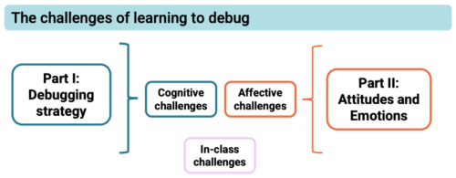
Laurie has spent the past two years talking to teachers and students and developing tools (a visualiser of students’ programming behaviour and PRIMMDebug, a teaching process and tool for debugging) to understand why many secondary school students struggle with debugging. It has quickly become clear through his research that most issues are due to problematic debugging strategies and students’ negative experiences and attitudes.

When students first start learning how to program, they have to remember a vast amount of new information, such as different variables, concepts, and program designs. Utilising this knowledge is often challenging because they’re already busy juggling all the content they’ve previously learnt and the challenges of the programming task at hand. When error messages inevitably appear that are confusing or misunderstood, it can become extremely difficult to debug effectively.
Given this information overload, students often don’t develop efficient strategies for debugging. When Laurie analysed the debugging efforts of 12- to 14-year-old secondary school students, he noticed some interesting differences between students who were more and less successful at debugging. While successful students generally seemed to make less frequent and more intentional changes, less successful students tinkered frequently with their broken programs, making one- or two-character edits before running the program again. In addition, the less successful students often ran the program soon after beginning the debugging exercise without allowing enough time to actually read the code and understand what it was meant to do.
The issue with these behaviours was that they often resulted in students adding errors when changing the program, which then compounded and made debugging increasingly difficult with each run. 74% of students also resorted to spamming, pressing ‘run’ again and again without changing anything. This strategy resonated with many of our seminar attendees, who reported doing the same thing after becoming frustrated.
Educators need to be aware of the negative consequences of students’ exasperating and often overwhelming experiences with debugging, especially if students are less confident in their programming skills to begin with. Even though spending 15 minutes on an exercise shows a remarkable level of tenaciousness and resilience, students’ attitudes to programming — and computing as a whole — can quickly go downhill if their strategies for identifying errors prove ineffective. Debugging becomes a vicious circle: if a student has negative experiences, they are less confident when having to bug-fix again in the future, which can lead to another set of unsuccessful attempts, which can further damage their confidence, and so on. Avoiding this downward spiral is essential.
Approaches to help students engage with debugging
Laurie stresses the importance of understanding the cognitive challenges of debugging and using the right tools and techniques to empower students and support them in developing effective strategies.
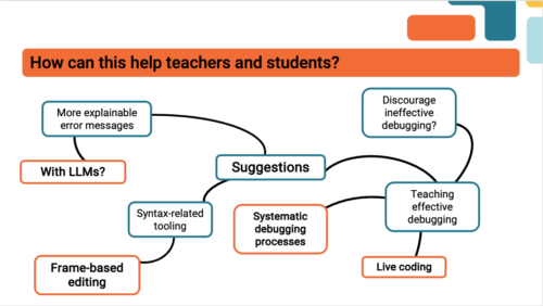
Some ideas of how to improve debugging skills that were mentioned by Laurie and our attendees included:
- Using frame-based editing tools for novice programmers because such tools encourage students to focus on logical errors rather than accidental syntax errors, which can distract them from understanding the issues with the program. Teaching debugging should also go hand in hand with understanding programming syntax and using simple language. As one of our attendees put it, “You wouldn’t give novice readers a huge essay and ask them to find errors.”
- Making error messages more understandable, for example, by explaining them to students using Large Language Models.
- Teaching systematic debugging processes. There are several different approaches to doing this. One of our participants suggested using the scientific method (forming a hypothesis about what is going wrong, devising an experiment that will provide information to see whether the hypothesis is right, and iterating this process) to methodically understand the program and its bugs.
Most importantly, debugging should not be a daunting or stressful experience. Everyone in the seminar agreed that creating a positive error culture is essential.
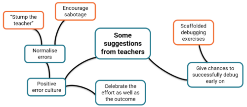
Some ideas you could explore in your classroom include:
- Normalising errors: Stress how normal and important program errors are. Everyone encounters them — a professional software developer in our audience said that they spend about half of their time debugging.
- Rewarding perseverance: Celebrate the effort, not just the outcome.
- Modelling how to fix errors: Let your students write buggy programs and attempt to debug them in front of the class.
In a welcoming classroom where students are given support and encouragement, debugging can be a rewarding experience. What may at first appear to be a failure — even a spectacular one — can be embraced as a valuable opportunity for learning. As a teacher in Laurie’s study said, “If something should have gone right and went badly wrong but somebody found something interesting on the way… you celebrate it. Take the fear out of it.”
Watch the recording of Laurie’s presentation:
Join our next seminar
In our current seminar series, we are exploring how to teach programming with and without AI.
Join us at our next seminar on Tuesday, 12 November at 17:00–18:30 GMT to hear Nicholas Gardella (University of Virginia) discuss the effects of using tools like GitHub Copilot on the motivation, workload, emotion, and self-efficacy of novice programmers. To sign up and take part in the seminar, click the button below — we’ll then send you information about joining. We hope to see you there.
The schedule of our upcoming seminars is online. You can catch up on past seminars on our previous seminars and recordings page.
The post How to make debugging a positive experience for secondary school students appeared first on Raspberry Pi Foundation.
Comic for 2024.10.15 – Grandpa
Post Syndicated from Explosm.net original https://explosm.net/comics/grandpa
New Cyanide and Happiness Comic
The Last Bonaparte Emperor
Post Syndicated from The History Guy: History Deserves to Be Remembered original https://www.youtube.com/watch?v=OBWRrSQ-OGA
Learn how to deploy Falcon 2 11B on Amazon EC2 c7i instances for model Inference
Post Syndicated from Anusha Jampala original https://aws.amazon.com/blogs/compute/learn-how-to-deploy-falcon-2-11b-on-amazon-ec2-c7i-instances-for-model-inference/
This post is written by Paul Tran, Senior Specialist SA; Asif Mujawar, Specialist SA Leader; Abdullatif AlRashdan, Specialist SA; and Shivagami Gugan, Enterprise Technologist.
Technology Innovation Institute (TII) has developed Falcon 2 11B foundation model (FM), a next-generation AI model that can be now deployed on Amazon Elastic Compute Cloud (Amazon EC2) c7i instances, which support Intel Advanced Matrix Extensions (Intel AMX). Intel AMX is designed to accelerate matrix operations on a CPU, which is fundamental for deep learning and AI workloads.
This post walks through the concept of model quantization and why quantization is vital for real-time use cases. You will be able to reproduce this process and run the model on a CPU at the end of this post.
Open source developers and customers can now use the EC2 C7i instance family to run their AI-powered applications using the Falcon 2 11B model on a CPU, offering a cost-effective alternative to the traditional GPU route to build cost-efficient solutions. It also unlocks deployment of the large language model (LLM) on widely available hardware that enables deployment of efficient and scalable AI applications.
Falcon 2 11B model
Falcon 2 11B is the first FM model from TII’s newly released Falcon 2 series. It is a more efficient and accessible LLM that was trained on a massive dataset of 5.5 trillion tokens consisting of web data from RefinedWeb. The model is built on causal decoder-only architecture with 11 billion trainable parameters, making it powerful for autoregressive tasks. It’s equipped with multilingual capabilities and can seamlessly tackle tasks in English, French, Spanish, German, Portuguese, and other languages for diverse scenarios. The new Falcon 2 Series, trained on Amazon SageMaker, widens the capabilities of Falcon by making it more efficient and multilingual. More detailed information on the previous generation of Falcon models can be found at RefinedWeb, Falcon 40B foundation model from TII available on SageMaker JumpStart, and Falcon 180B foundation model from TII is now available via Amazon SageMaker JumpStart.
Falcon 2 11B is supported by the Amazon SageMaker Text Generation Inference (TGI) Deep Learning Container (DLC), an open source, purpose-built solution for deploying and serving LLMs that enables high performance text generation using tensor parallelism and dynamic batching. The model is available under the TII Falcon License 2.0, the permissive Apache 2.0-based software license, which includes an acceptable use policy that promotes the responsible use of AI. In addition, Falcon 2 11B is now available on Amazon SageMaker JumpStart.
INT8 and INT4 quantization
For real-time applications such as Retrieval Augmented Generation (RAG) or code generation, reducing the latency for generating the first token is crucial, and minimizing the time between generating subsequent tokens promotes a seamless experience. These benefits are essential for applications that require real-time interaction, where even minor delays could disrupt the user experience and hinder productivity.
The OpenVINO framework enables INT8 and INT4 quantization and weight compression. This optimizes performance by reducing the model size and computational demands, making generative AI more cost-effective. These optimizations lower inference cost while maintaining high quality outputs.
Intel AMX is a new built-in accelerator that improves the performance of deep learning training and inference on the CPU. It provides significant performance advantages for INT8 and INT4 inferencing by accelerating matrix multiplication for deep learning workloads, which are essential in AI model execution. By using AMX, INT8 and INT4 precision models can run faster and more efficiently, without substantial loss in accuracy, providing for quicker inference and lower power consumption.
Benchmark results summary
The C7i.24xlarge instance was used for benchmarking the inference performance of the Falcon 2 11B model. The results showcased the effectiveness of INT8 and INT4 quantization techniques, using the OpenVINO toolkit. The results demonstrate significant improvements in latency and throughput.
The code to reproduce the benchmarks on the c7i instance can be found at openvino.genai. Please note that benchmarking performance varies by use, configuration, and other factors.
Case 1
Quantization technique using INT8 Falcon 2 11B with OpenVINO on c7i.24xlarge.
| Quantization | Batch |
Input prompt tokens |
Output tokens |
First token latency ms/token |
Second token latency ms/token | Throughput tokens/s |
| INT8 | 1 | 32 | 128 | 148.07 | 82.51 | 12.12 |
| INT8 | 1 | 64 | 128 | 189.98 | 79.74 | 12.54 |
| INT8 | 1 | 128 | 128 | 283.50 | 80.26 | 12.46 |
| INT8 | 1 | 512 | 128 | 1037.25 | 82.03 | 12.19 |
| INT8 | 1 | 1024 | 128 | 1961.91 | 84.76 | 11.80 |
| INT8 | 1 | 2048 | 128 | 4068.90 | 90.40 | 11.06 |
Table 1: Quantization technique using INT8 Falcon 2 11B with OpenVINO on c7i.24xlarge
Case 2
Quantization technique using INT4 Falcon11B with OpenVINO on c7i.24xlarge.
| Quantization | Batch |
Input prompt tokens |
Output tokens |
First token latency ms/token | Second token latency ms/token | Throughput tokens/s |
| INT4 | 1 | 32 | 128 | 142.00 | 59.06 | 16.93 |
| INT4 | 1 | 64 | 128 | 195.73 | 82.58 | 12.11 |
| INT4 | 1 | 128 | 128 | 274.67 | 80.40 | 12.44 |
| INT4 | 1 | 512 | 128 | 991.34 | 82.22 | 12.16 |
| INT4 | 1 | 1024 | 128 | 1922.87 | 85.18 | 11.74 |
| INT4 | 1 | 2048 | 128 | 4079.58 | 90.11 | 11.10 |
As these results show, INT8 quantization provides excellent latency and throughput numbers. This demonstrates how suitable inference on a CPU is for real-time use cases such as RAG or code generation. Increased performance can also be obtained with more aggressive quantization, such as INT4.
AWS customers can now explore and deploy Falcon 2 11B models using c7i instances across AWS Regions with dedicated performance improvements using OpenVINO Toolkit.
Quantize Falcon 2 11B using OpenVINO and run inference
Developers can use the following approach to quantize Falcon 2 11B and optimize to run on CPU instances. The model is pulled from HuggingFace hub through the OpenVINO framework. A full list of compatible models can be found at AI Models verified for OpenVINO.
For the model quantization, the process requires large RAM memory peaking up to over 116 GB for 11 billion parameters at full precision, hence the choice of running the experiments on c7i.24xlarge equipped with 192 GB of RAM for convenience.
This is shown in the following figure during quantization.

Figure 1: Model quantization
Once quantization is achieved, the converted model weights are stored in the instance disk ready to be consumed for inference.
The inference memory requirement is lower compared to the quantization process because the memory footprint of the quantized model for inference is approximately 12 GB, as illustrated in following figure. Running the inference on the c7i.24xlarge instance allows you to benefit from the increased number of cores, which directly correlates with model speed.

Figure 2: Memory footprint of quantized model for inference
Quantize Falcon 2 11B
To quantize Falcon 2 11B using OpenVINO, complete the following steps:
1. Create c7i.24xlarge EC2 instance in your AWS account.
2. Size the Amazon Elastic Block Store (Amazon EBS) storage depending on the number of models you need to experiment with. For instance, using Falcon 2 11B model weights at full precision requires approximately 24 GB of storage. For comfort, we recommend running with at least 150 GB of storage to experiment with different precisions and models.
3. Connect to your EC2 instance. See Connect to your EC2 instance to see the different options you can use to access your EC2 instance.
4. Create a virtual environment using the following code example.
python3 -m venv ov-llm-bench-env
source ov-llm-bench-env/bin/activate
pip install --upgrade pipClone the repository and navigate to the source directory.
5. Clone repository and navigate to the source directory:
git clone https://github.com/openvinotoolkit/openvino.genai.git
cd openvino.genai/llm_bench/python/
6. Install dependencies:
pip install -r requirements.txt7. Run model conversion:
python convert.py --model_id tiiuae/falcon-11B --output_dir model_weights/int8/ --compress_weights INT8 4BIT_DEFAULTThis command perform quantization using OpenVINO on Falcon2-11B model. It downloads the model from HuggingFace and output the converted model in the path specified in -output_dir
Test Falcon2-11B for inference
OpenVINO provides a convenient interface that allows to use the model with HuggingFace transformers library. Run the following python script on your EC2 instance to test inference:
from transformers import AutoTokenizer
from optimum.intel.openvino import OVModelForCausalLM

if __name__ == '__main__':
    model_path= "model_weights/int8/pytorch/dldt/compressed_weights/OV_FP32-INT8/"
    tokenizer = AutoTokenizer.from_pretrained(model_path)
    model = OVModelForCausalLM.from_pretrained(model_path)

    inputs = tokenizer("What is OpenVINO?", return_tensors="pt")

    outputs = model.generate(**inputs, max_length=200)
    text = tokenizer.batch_decode(outputs)[0]
    print(text)# Falcon2-11B inference completion
The following screenshot shows a sample generated from the previous code. The output is truncated to generate 200 tokens maximum.

Figure 3: Inference results after running Python script
Conclusion
In this post, we showcased Falcon 2 11B quantization and optimized performance using OpenVINO on AMX capable EC2 c7i instances. This enables deployment of LLM-based applications on widely available CPUs with high performance as a cost-effective alternative without sacrificing speed. These optimizations significantly lower inference costs while maintaining high-quality outputs.
For more information, refer to Amazon EC2 C7i and C7i-flex instances, SageMaker JumpStart pre-trained models, Amazon SageMaker JumpStart Foundation Models, OpenVINO, and the reference code for quantization.
Leave your feedback in the comments so we can continue to improve upon this benchmark.
AMD Pensando Pollara 400 UltraEthernet RDMA NIC Launched
Post Syndicated from Patrick Kennedy original https://www.servethehome.com/amd-pensando-pollara-400-ultraethernet-rdma-nic-launched/
The new AMD Pensando Pollara 400 is a 400GBE UltraEthernet Consortium RDMA NIC designed for AI servers and next-gen UEC networks
The post AMD Pensando Pollara 400 UltraEthernet RDMA NIC Launched appeared first on ServeTheHome.
Investigation of a Workbench UI Latency Issue
Post Syndicated from Netflix Technology Blog original https://netflixtechblog.com/investigation-of-a-workbench-ui-latency-issue-faa017b4653d
By: Hechao Li and Marcelo Mayworm
With special thanks to our stunning colleagues Amer Ather, Itay Dafna, Luca Pozzi, Matheus Leão, and Ye Ji.
Overview
At Netflix, the Analytics and Developer Experience organization, part of the Data Platform, offers a product called Workbench. Workbench is a remote development workspace based on Titus that allows data practitioners to work with big data and machine learning use cases at scale. A common use case for Workbench is running JupyterLab Notebooks.
Recently, several users reported that their JupyterLab UI becomes slow and unresponsive when running certain notebooks. This document details the intriguing process of debugging this issue, all the way from the UI down to the Linux kernel.
Symptom
Machine Learning engineer Luca Pozzi reported to our Data Platform team that their JupyterLab UI on their workbench becomes slow and unresponsive when running some of their Notebooks. Restarting the ipykernel process, which runs the Notebook, might temporarily alleviate the problem, but the frustration persists as more notebooks are run.
Quantify the Slowness
While we observed the issue firsthand, the term “UI being slow” is subjective and difficult to measure. To investigate this issue, we needed a quantitative analysis of the slowness.
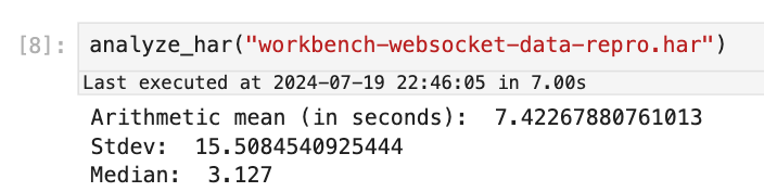
Itay Dafna devised an effective and simple method to quantify the UI slowness. Specifically, we opened a terminal via JupyterLab and held down a key (e.g., “j”) for 15 seconds while running the user’s notebook. The input to stdin is sent to the backend (i.e., JupyterLab) via a WebSocket, and the output to stdout is sent back from the backend and displayed on the UI. We then exported the .har file recording all communications from the browser and loaded it into a Notebook for analysis.

Using this approach, we observed latencies ranging from 1 to 10 seconds, averaging 7.4 seconds.
Blame The Notebook
Now that we have an objective metric for the slowness, let’s officially start our investigation. If you have read the symptom carefully, you must have noticed that the slowness only occurs when the user runs certain notebooks but not others.
Therefore, the first step is scrutinizing the specific Notebook experiencing the issue. Why does the UI always slow down after running this particular Notebook? Naturally, you would think that there must be something wrong with the code running in it.
Upon closely examining the user’s Notebook, we noticed a library called pystan , which provides Python bindings to a native C++ library called stan, looked suspicious. Specifically, pystan uses asyncio. However, because there is already an existing asyncio event loop running in the Notebook process and asyncio cannot be nested by design, in order for pystan to work, the authors of pystan recommend injecting pystan into the existing event loop by using a package called nest_asyncio, a library that became unmaintained because the author unfortunately passed away.
Given this seemingly hacky usage, we naturally suspected that the events injected by pystan into the event loop were blocking the handling of the WebSocket messages used to communicate with the JupyterLab UI. This reasoning sounds very plausible. However, the user claimed that there were cases when a Notebook not using pystan runs, the UI also became slow.
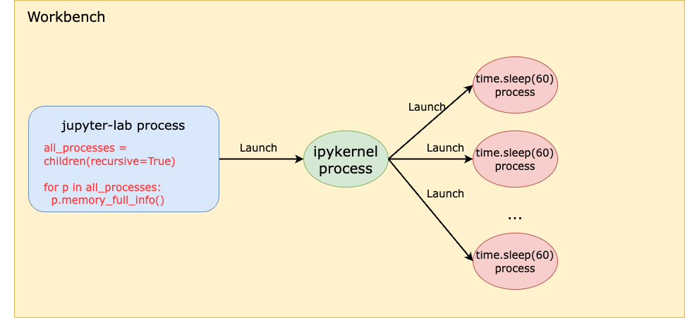
Moreover, after several rounds of discussion with ChatGPT, we learned more about the architecture and realized that, in theory, the usage of pystan and nest_asyncio should not cause the slowness in handling the UI WebSocket for the following reasons:
Even though pystan uses nest_asyncio to inject itself into the main event loop, the Notebook runs on a child process (i.e., the ipykernel process) of the jupyter-lab server process, which means the main event loop being injected by pystan is that of the ipykernel process, not the jupyter-server process. Therefore, even if pystan blocks the event loop, it shouldn’t impact the jupyter-lab main event loop that is used for UI websocket communication. See the diagram below:
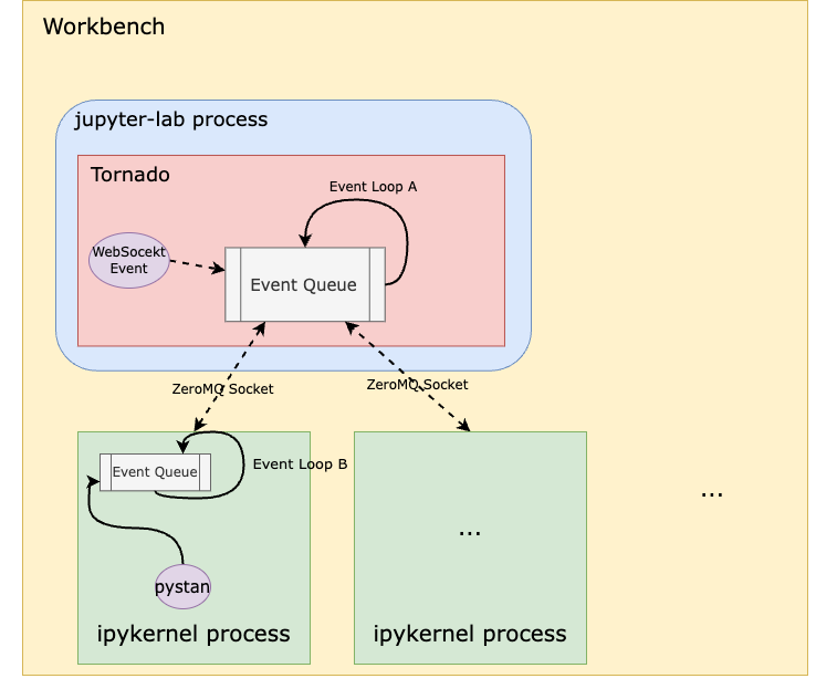
In other words, pystan events are injected to the event loop B in this diagram instead of event loop A. So, it shouldn’t block the UI WebSocket events.
You might also think that because event loop A handles both the WebSocket events from the UI and the ZeroMQ socket events from the ipykernel process, a high volume of ZeroMQ events generated by the notebook could block the WebSocket. However, when we captured packets on the ZeroMQ socket while reproducing the issue, we didn’t observe heavy traffic on this socket that could cause such blocking.
A stronger piece of evidence to rule out pystan was that we were ultimately able to reproduce the issue even without it, which I’ll dive into later.
Blame Noisy Neighbors
The Workbench instance runs as a Titus container. To efficiently utilize our compute resources, Titus employs a CPU oversubscription feature, meaning the combined virtual CPUs allocated to containers exceed the number of available physical CPUs on a Titus agent. If a container is unfortunate enough to be scheduled alongside other “noisy” containers — those that consume a lot of CPU resources — it could suffer from CPU deficiency.
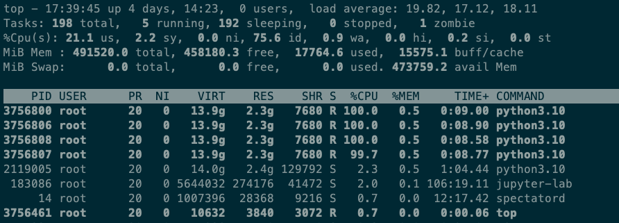
However, after examining the CPU utilization of neighboring containers on the same Titus agent as the Workbench instance, as well as the overall CPU utilization of the Titus agent, we quickly ruled out this hypothesis. Using the top command on the Workbench, we observed that when running the Notebook, the Workbench instance uses only 4 out of the 64 CPUs allocated to it. Simply put, this workload is not CPU-bound.
Blame The Network
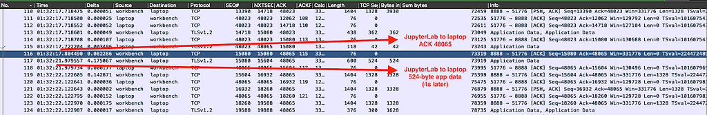
The next theory was that the network between the web browser UI (on the laptop) and the JupyterLab server was slow. To investigate, we captured all the packets between the laptop and the server while running the Notebook and continuously pressing ‘j’ in the terminal.
When the UI experienced delays, we observed a 5-second pause in packet transmission from server port 8888 to the laptop. Meanwhile, traffic from other ports, such as port 22 for SSH, remained unaffected. This led us to conclude that the pause was caused by the application running on port 8888 (i.e., the JupyterLab process) rather than the network.
The Minimal Reproduction
As previously mentioned, another strong piece of evidence proving the innocence of pystan was that we could reproduce the issue without it. By gradually stripping down the “bad” Notebook, we eventually arrived at a minimal snippet of code that reproduces the issue without any third-party dependencies or complex logic:
import time
import os
from multiprocessing import Process

N = os.cpu_count()

def launch_worker(worker_id):
  time.sleep(60)

if __name__ == '__main__':
  with open('/root/2GB_file', 'r') as file:
    data = file.read()
    processes = []
    for i in range(N):
      p = Process(target=launch_worker, args=(i,))
      processes.append(p)
      p.start()

    for p in processes:
      p.join()
The code does only two things:
- Read a 2GB file into memory (the Workbench instance has 480G memory in total so this memory usage is almost negligible).
- Start N processes where N is the number of CPUs. The N processes do nothing but sleep.
There is no doubt that this is the most silly piece of code I’ve ever written. It is neither CPU bound nor memory bound. Yet it can cause the JupyterLab UI to stall for as many as 10 seconds!
Questions
There are a couple of interesting observations that raise several questions:
- We noticed that both steps are required in order to reproduce the issue. If you don’t read the 2GB file (that is not even used!), the issue is not reproducible. Why using 2GB out of 480GB memory could impact the performance?
- When the UI delay occurs, the jupyter-lab process CPU utilization spikes to 100%, hinting at contention on the single-threaded event loop in this process (event loop A in the diagram before). What does the jupyter-lab process need the CPU for, given that it is not the process that runs the Notebook?
- The code runs in a Notebook, which means it runs in the ipykernel process, that is a child process of the jupyter-lab process. How can anything that happens in a child process cause the parent process to have CPU contention?
- The workbench has 64CPUs. But when we printed os.cpu_count(), the output was 96. That means the code starts more processes than the number of CPUs. Why is that?
Let’s answer the last question first. In fact, if you run lscpu and nproc commands inside a Titus container, you will also see different results — the former gives you 96, which is the number of physical CPUs on the Titus agent, whereas the latter gives you 64, which is the number of virtual CPUs allocated to the container. This discrepancy is due to the lack of a “CPU namespace” in the Linux kernel, causing the number of physical CPUs to be leaked to the container when calling certain functions to get the CPU count. The assumption here is that Python os.cpu_count() uses the same function as the lscpu command, causing it to get the CPU count of the host instead of the container. Python 3.13 has a new call that can be used to get the accurate CPU count, but it’s not GA’ed yet.
It will be proven later that this inaccurate number of CPUs can be a contributing factor to the slowness.
More Clues
Next, we used py-spy to do a profiling of the jupyter-lab process. Note that we profiled the parent jupyter-lab process, not the ipykernel child process that runs the reproduction code. The profiling result is as follows:
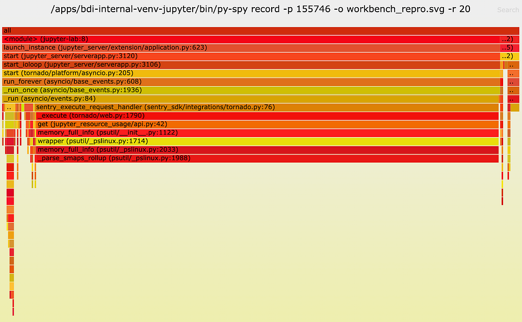
As one can see, a lot of CPU time (89%!!) is spent on a function called __parse_smaps_rollup. In comparison, the terminal handler used only 0.47% CPU time. From the stack trace, we see that this function is inside the event loop A, so it can definitely cause the UI WebSocket events to be delayed.
The stack trace also shows that this function is ultimately called by a function used by a Jupyter lab extension called jupyter_resource_usage. We then disabled this extension and restarted the jupyter-lab process. As you may have guessed, we could no longer reproduce the slowness!
But our puzzle is not solved yet. Why does this extension cause the UI to slow down? Let’s keep digging.
Root Cause Analysis
From the name of the extension and the names of the other functions it calls, we can infer that this extension is used to get resources such as CPU and memory usage information. Examining the code, we see that this function call stack is triggered when an API endpoint /metrics/v1 is called from the UI. The UI apparently calls this function periodically, according to the network traffic tab in Chrome’s Developer Tools.
Now let’s look at the implementation starting from the call get(jupter_resource_usage/api.py:42) . The full code is here and the key lines are shown below:
cur_process = psutil.Process()
all_processes = [cur_process] + cur_process.children(recursive=True)

for p in all_processes:
  info = p.memory_full_info()
Basically, it gets all children processes of the jupyter-lab process recursively, including both the ipykernel Notebook process and all processes created by the Notebook. Obviously, the cost of this function is linear to the number of all children processes. In the reproduction code, we create 96 processes. So here we will have at least 96 (sleep processes) + 1 (ipykernel process) + 1 (jupyter-lab process) = 98 processes when it should actually be 64 (allocated CPUs) + 1 (ipykernel process) + 1 (jupyter-lab process) = 66 processes, because the number of CPUs allocated to the container is, in fact, 64.
This is truly ironic. The more CPUs we have, the slower we are!
At this point, we have answered one question: Why does starting many grandchildren processes in the child process cause the parent process to be slow? Because the parent process runs a function that’s linear to the number all children process recursively.
However, this solves only half of the puzzle. If you remember the previous analysis, starting many child processes ALONE doesn’t reproduce the issue. If we don’t read the 2GB file, even if we create 2x more processes, we can’t reproduce the slowness.
So now we must answer the next question: Why does reading a 2GB file in the child process affect the parent process performance, especially when the workbench has as much as 480GB memory in total?
To answer this question, let’s look closely at the function __parse_smaps_rollup. As the name implies, this function parses the file /proc/<pid>/smaps_rollup.
def _parse_smaps_rollup(self):
  uss = pss = swap = 0
  with open_binary("{}/{}/smaps_rollup".format(self._procfs_path, self.pid)) as f:
  for line in f:
    if line.startswith(b”Private_”):
    # Private_Clean, Private_Dirty, Private_Hugetlb
      s uss += int(line.split()[1]) * 1024
    elif line.startswith(b”Pss:”):
      pss = int(line.split()[1]) * 1024
    elif line.startswith(b”Swap:”):
      swap = int(line.split()[1]) * 1024
return (uss, pss, swap)
Naturally, you might think that when memory usage increases, this file becomes larger in size, causing the function to take longer to parse. Unfortunately, this is not the answer because:
- First, the number of lines in this file is constant for all processes.
- Second, this is a special file in the /proc filesystem, which should be seen as a kernel interface instead of a regular file on disk. In other words, I/O operations of this file are handled by the kernel rather than disk.
This file was introduced in this commit in 2017, with the purpose of improving the performance of user programs that determine aggregate memory statistics. Let’s first focus on the handler of open syscall on this /proc/<pid>/smaps_rollup.
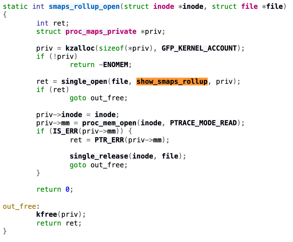
Following through the single_open function, we will find that it uses the function show_smaps_rollup for the show operation, which can translate to the read system call on the file. Next, we look at the show_smaps_rollup implementation. You will notice a do-while loop that is linear to the virtual memory area.
static int show_smaps_rollup(struct seq_file *m, void *v) {
  …
  vma_start = vma->vm_start;
  do {
    smap_gather_stats(vma, &mss, 0);
    last_vma_end = vma->vm_end;
    …
  } for_each_vma(vmi, vma);
  …
}
This perfectly explains why the function gets slower when a 2GB file is read into memory. Because the handler of reading the smaps_rollup file now takes longer to run the while loop. Basically, even though smaps_rollup already improved the performance of getting memory information compared to the old method of parsing the /proc/<pid>/smaps file, it is still linear to the virtual memory used.
More Quantitative Analysis
Even though at this point the puzzle is solved, let’s conduct a more quantitative analysis. How much is the time difference when reading the smaps_rollup file with small versus large virtual memory utilization? Let’s write some simple benchmark code like below:
import os

def read_smaps_rollup(pid):
  with open("/proc/{}/smaps_rollup".format(pid), "rb") as f:
    for line in f:
      pass

if __name__ == “__main__”:
  pid = os.getpid()

  read_smaps_rollup(pid)

  with open(“/root/2G_file”, “rb”) as f:
    data = f.read()

  read_smaps_rollup(pid)
This program performs the following steps:
- Reads the smaps_rollup file of the current process.
- Reads a 2GB file into memory.
- Repeats step 1.
We then use strace to find the accurate time of reading the smaps_rollup file.
$ sudo strace -T -e trace=openat,read python3 benchmark.py 2>&1 | grep “smaps_rollup” -A 1

openat(AT_FDCWD, “/proc/3107492/smaps_rollup”, O_RDONLY|O_CLOEXEC) = 3 <0.000023>
read(3, “560b42ed4000–7ffdadcef000 — -p 0”…, 1024) = 670 <0.000259>
...
openat(AT_FDCWD, “/proc/3107492/smaps_rollup”, O_RDONLY|O_CLOEXEC) = 3 <0.000029>
read(3, “560b42ed4000–7ffdadcef000 — -p 0”…, 1024) = 670 <0.027698>
As you can see, both times, the read syscall returned 670, meaning the file size remained the same at 670 bytes. However, the time it took the second time (i.e., 0.027698 seconds) is 100x the time it took the first time (i.e., 0.000259 seconds)! This means that if there are 98 processes, the time spent on reading this file alone will be 98 * 0.027698 = 2.7 seconds! Such a delay can significantly affect the UI experience.
Solution
This extension is used to display the CPU and memory usage of the notebook process on the bar at the bottom of the Notebook:

We confirmed with the user that disabling the jupyter-resource-usage extension meets their requirements for UI responsiveness, and that this extension is not critical to their use case. Therefore, we provided a way for them to disable the extension.
Summary
This was such a challenging issue that required debugging from the UI all the way down to the Linux kernel. It is fascinating that the problem is linear to both the number of CPUs and the virtual memory size — two dimensions that are generally viewed separately.
Overall, we hope you enjoyed the irony of:
- The extension used to monitor CPU usage causing CPU contention.
- An interesting case where the more CPUs you have, the slower you get!
If you’re excited by tackling such technical challenges and have the opportunity to solve complex technical challenges and drive innovation, consider joining our Data Platform teams. Be part of shaping the future of Data Security and Infrastructure, Data Developer Experience, Analytics Infrastructure and Enablement, and more. Explore the impact you can make with us!
![]()
Investigation of a Workbench UI Latency Issue was originally published in Netflix TechBlog on Medium, where people are continuing the conversation by highlighting and responding to this story.
Inkscape 1.4 released
Post Syndicated from jzb original https://lwn.net/Articles/994098/
Version
1.4 of the Inkscape
open-source vector-graphics editor has been released. Highlights of
this release include a filter gallery, import for Affinity Designer
files, internal links in exported PDFs, and more. See the release
notes for all of the new features. LWN previewed the 1.4 release
in early October.
[$] WordPress retaliation impacts community
Post Syndicated from jzb original https://lwn.net/Articles/993895/
It is too early to say what the outcome will be in the ongoing fight between Automattic and WP Engine, but the WordPress community at large is already the
loser. Automattic founder and CEO Matt Mullenweg has been using
his control of the project, and the WordPress.org infrastructure, to
punish WP Engine and remove some dissenting contributors from discussion
channels. Most recently, Mullenweg has instituted a hostile fork of a
WP Engine plugin and the forked plugin is replacing the original
via WordPress updates.
AWS Weekly Roundup: What’s App, AWS Lambda, Load Balancers, AWS Console, and more (Oct 14, 2024).
Post Syndicated from Sébastien Stormacq original https://aws.amazon.com/blogs/aws/aws-weekly-roundup-whats-app-aws-lambda-load-balancers-aws-console-and-more-oct-14-2024/
Last week, AWS hosted free half-day conferences in London and Paris. My colleagues and I demonstrated how developers can use generative AI tools to speed up their design, analysis, code writing, debugging, and deployment workflows. These events were held at the GenAI Lofts. These lofts are open until October 25 (London) and November 5 (Paris). They will be packed with events, conferences, workshops, and meetups. If you’re around, be sure to check the agenda (London, Paris).
 |
 |
Our well-known AWS News blog co-author Veliswa did an amazing demo. She live-coded a Duolingo-like app from scratch, just using suggestions and reviews from Amazon Q Developer.
Now, let’s turn to other exciting news in the AWS universe from last week.
Last week’s launches
Here are some launches that got my attention:
Bring your conversations to WhatsApp — AWS has added support for What’sApp to AWS End User Messaging, so developers can reach users on WhatsApp with multimedia and interactive messaging options. This feature integrates with SMS and push notifications already available. Developers can get started quickly using AWS Management Console.
Amazon Redshift data sharing with data lake tables — This offers a secure and convenient way to share live data lake tables across different Amazon Redshift warehouses. Data sharing of data lake tables in AWS Glue Data Catalog provides live access to the data, so you always see the most up-to-date and consistent information as it’s updated in the data lake.
Zonal shift and zonal autoshift for cross zoned Network Load Balancer — Network Load Balancer (NLB) now supports the Amazon Application Recovery Controller zonal shift and zonal autoshift features on load balancers that are enabled across zones. With Zonal shift, you can quickly shift traffic away from an impaired Availability Zone and recover from events such as bad application deployment and gray failures. Zonal autoshift safely and automatically shifts your traffic away from an Availability Zone when AWS identifies a potential impact to it.
Console to Code to generate infrastructure as a service code — This is by far my favorite launch of the week. Console to Code makes it simple, fast, and cost-effective to move from prototyping in the AWS Management Console to building code for production deployments. You can generate code for their console actions in their preferred format with a single click. The generated code helps you get started and bootstrap your automation pipelines for tasks. Console to Code is powered by Amazon Q Developer.
A new getting started experience for AWS CodePipeline — AWS Data Pipeline introduces a simplified and new getting started experience so you can quickly create new pipelines. When you create a new pipeline using the CodePipeline console, you can now select from a list of pipeline templates across build, automation, and deployment use cases. After selecting a pipeline template, you will be prompted to enter values for the action configuration fields in the pipeline definition, and completing the process will render a fully configured pipeline that’s ready to run.
AWS Lambda detects and stops recursive loops between Lambda and Amazon S3 — Lambda recursive loop detection can now automatically detect and stop recursive loops between AWS Lambda and Amazon Simple Storage Service (Amazon S3). Lambda recursive loop detection, which is enabled by default, is a preventative guardrail that automatically detects and stops recursive invocations between Lambda and other supported services, preventing unintended usage and billing from runaway workloads.
Amazon MemoryDB for Valkey — Amazon MemoryDB for Redis is a fully managed, Valkey– and Redis OSS-compatible database service, which provides multi-AZ durability, microsecond read and single-digit millisecond write latency, and high throughput. It is ideal for use cases such as caching, leaderboards, and session stores. With MemoryDB for Valkey, you can benefit from a fully managed experience built on open-source technology while using the security, operational excellence, and reliability that AWS provides. MemoryDB for Valkey also delivers the fastest vector search performance at the highest recall rates among popular vector databases on AWS.
Amazon Polly adds four wew English voices for the generative engine and expands to three Regions — Polly is a managed service that turns text into lifelike speech, so you can create applications that talk and to build speech-enabled products depending on your business needs. The generative engine is the most advanced Amazon Polly text-to-speech (TTS) model. With this launch, we add a variety of new synthetic generative English voices to the Amazon Polly portfolio: an Australian English voice Olivia and three US English voices Joanna, Danielle, and Stephen. These voices have more natural pronunciation and prosody. You can use this high-tier product in various industries and for different purposes such as education, publishing, or marketing.
For a full list of AWS announcements, be sure to keep an eye on the AWS What’s New Feed page.
Upcoming AWS events
Check your calendars and sign up for these AWS events:
AWS Cloud Day Prague — Join us for a free technical conferences in Prague on October 23. I will be there and share with attendees “The Art of Transforming a Foundation Model into a Domain Expert”. Be sure to register today!
Innovate Migrate, Modernize, and Build — Whether you are new to the cloud or an experienced user, you will learn something new at AWS Innovate. This is a free online conference. Register for a time and region convenient to North America (October 15), or Europe, Middle East & Africa (October 24).
AWS Community Days — Join community-led conferences featuring technical discussions, workshops, and hands-on labs led by expert AWS users and industry leaders from around the world. Don’t miss out on the AWS Community Days happening on October 19 in Vadodara, Spain, and Guatemala.
AWS re:Invent 2024 — Registration is now open for the annual tech extravaganza, taking place December 2 – 6 in Las Vegas. Beside recording podcast episodes, I will present three sessions:
- CMP410 | Accelerate testing cycles of CI/CD pipelines with EC2 Mac instances (with Vishal)
- DEV301 | The art of transforming foundation models into domain experts (with Gregory)
- DEV334 | Swift, server-side, serverless
There are just a few seats left for these three sessions, so be sure to book your seat today!
Browse more upcoming AWS led in-person and virtual events and developer-focused events.
That’s all for this week. Check back next Monday for another Weekly Roundup!
This post is part of our Weekly Roundup series. Check back each week for a quick roundup of interesting news and announcements from AWS!
Upcoming Speaking Engagements
Post Syndicated from B. Schneier original https://www.schneier.com/blog/archives/2024/10/upcoming-speaking-engagements-41.html
This is a current list of where and when I am scheduled to speak:
- I’m speaking at SOSS Fusion 2024 in Atlanta, Georgia, USA. The event will be held on October 22 and 23, 2024, and my talk is at 9:15 AM ET on October 22, 2024.
The list is maintained on this page.
Enriching metadata for accurate text-to-SQL generation for Amazon Athena
Post Syndicated from Naidu Rongali original https://aws.amazon.com/blogs/big-data/enriching-metadata-for-accurate-text-to-sql-generation-for-amazon-athena/
Extracting valuable insights from massive datasets is essential for businesses striving to gain a competitive edge. Enterprise data is brought into data lakes and data warehouses to carry out analytical, reporting, and data science use cases using AWS analytical services like Amazon Athena, Amazon Redshift, Amazon EMR, and so on. Amazon Athena provides interactive analytics service for analyzing the data in Amazon Simple Storage Service (Amazon S3). Amazon Redshift is used to analyze structured and semi-structured data across data warehouses, operational databases, and data lakes. Amazon EMR provides a big data environment for data processing, interactive analysis, and machine learning using open source frameworks such as Apache Spark, Apache Hive, and Presto. These data processing and analytical services support Structured Query Language (SQL) to interact with the data.
Writing SQL queries requires not just remembering the SQL syntax rules, but also knowledge of the tables metadata, which is data about table schemas, relationships among the tables, and possible column values. Large language model (LLM)-based generative AI is a new technology trend for comprehending a large corpora of information and assisting with complex tasks. Can it also help write SQL queries? The answer is yes.
Generative AI models can translate natural language questions into valid SQL queries, a capability known as text-to-SQL generation. Although LLMs can generate syntactically correct SQL queries, they still need the table metadata for writing accurate SQL query. In this post, we demonstrate the critical role of metadata in text-to-SQL generation through an example implemented for Amazon Athena using Amazon Bedrock. We discuss the challenges in maintaining the metadata as well as ways to overcome those challenges and enrich the metadata.
Solution overview
This post demonstrates text-to-SQL generation for Athena using an example implemented using Amazon Bedrock. We use Anthropic’s Claude 2.1 foundation model (FM) in Amazon Bedrock as the LLM. Amazon Bedrock models are invoked using Amazon SageMaker. Working examples are designed to demonstrate how various details included in the metadata influences the SQL generated by the model. These examples use synthetic datasets created in AWS Glue and Amazon S3. After we review the significance of these metadata details, we’ll delve into the challenges encountered in gathering the required level of metadata. Subsequently, we’ll explore strategies for overcoming these challenges.
The examples implemented in the workflow are illustrated in the following diagram.

Figure 1. The solution architecture and workflow.
The workflow follows the following sequence:
- A user asks a text-based question which can be answered by querying relevant AWS Glue tables through Athena.
- Table metadata is fetched from AWS Glue.
- The tables’ metadata and SQL generating instructions are added to the prompt template. The Claude AI model is invoked by passing the prompt and the model parameters.
- The Claude AI model translates the user intent (question) to SQL based on the instructions and tables’ metadata.
- The generated Athena SQL query is run.
- The generated Athena SQL query and the SQL query results are returned to the user.
Prerequisites
These prerequisites are given If you want to try this example yourself. You can skip this prerequisites section if you want to understand the example without implementing it. The example centers on invoking Amazon Bedrock models using SageMaker, so we need to set up a few resources in an AWS Account. The relevant CloudFormation template, Jupyter Notebooks, and details of launching the necessary AWS services are covered in this section. The CloudFormation template creates the SageMaker instance with the necessary S3 bucket and IAM role permissions to run AWS Glue commands, Athena SQL, and invoke Amazon Bedrock AI models. The two Jupyter Notebooks (0_create_tables_with_metadata.ipynb and 1_text-to-sql-for-athena.ipynb) provide working code snippets to create the necessary tables and generate the SQL using the Claude AI model on Amazon Bedrock.
Granting Anthropic’s Claude permissions on Amazon Bedrock
- Have an AWS account and sign in using the AWS Management Console.
- Change the AWS Region to US West (Oregon).
- Navigate to the AWS Service Catalog console and choose Amazon Bedrock.
- On the Amazon Bedrock console, choose Model Access in the navigation pane.
- Choose Manage model access.
- Select the Claude
- Choose Request model access if you’re requesting the model access for the first time. Otherwise choose Save Changes.
Deploying the CloudFormation stack
![]()
After launching the CloudFormation stack:
- On the Create stack page, choose Next
- On the Specify stack details page, choose Next
- On the Configure stack options page, choose Next
- On the Review and create page, select I acknowledge that AWS CloudFormation might create IAM resources
- Choose Submit
Downloading Jupyter Notebooks to SageMaker
- In the AWS Management Console, choose the name of the currently displayed Region and change it to US West (Oregon).
- Navigate to the AWS Service Catalog console and choose Amazon SageMaker.
- On the Amazon SageMaker console, choose Notebook in the navigation pane.
- Choose Notebook instances.
- Select the SageMakerNotebookInstance created by the
texttosqlmetadataCloudFormation stack. - Under Actions, choose Open Jupyter
- Navigate to Jupyter console, select New, and then choose Console.
- Run the following Shell script commands in the console to copy the Jupyter Notebooks.
- Open each downloaded Notebook and update the values of the
athena_results_bucket, aws_region, andathena_workgroupvariables based on the outputs from thetexttosqlmetadataCloudFormation
Solution implementation
If you want to try this example yourself, try the CloudFormation template provided in the previous section. In the subsequent sections, we will illustrate how each element of the metadata included in the prompt influences the SQL query generated by the model.
- The steps in the
0_create_tables_with_metadata.ipynbJupyter Notebook create Amazon S3 files with synthetic data for employee and department datasets, createsemployee_dtlsanddepartment_dtlsGlue tables pointing to those S3 buckets, and extracts the following metadata for these two tables. - The metadata extracted in the previous step provides column descriptions. For the
region_idpartition column andemp_categorycolumn, the description provides possible values along with their meaning. The metadata also has foreign key constraint details. AWS Glue doesn’t provide a way to specify the primary key and foreign key constraints, so use custom keys in the AWS Glue table-level parameters as an alternative to gather primary key and foreign keys while creating the AWS Glue table. - The steps in the
1_text-to-sql-for-athena.ipynbJupyter notebook create the following wrapper function to interact with Claude FM on Amazon Bedrock to generate SQL based on user-provided text wrapped up in a prompt. This function hard codes the model’s parameters and model ID for demonstrating the basic functionality. - Define the following set of instructions for generating Athena SQL query. These SQL generating instructions specify which compute engine the SQL query should run on and other instructions to guide the model in generating the SQL query. These instructions are included in the prompt sent to the Bedrock model.
- Define different prompt templates for demonstrating the importance of metadata in text-to-SQL generation. These templates have placeholders for SQL query generating instructions and tables metadata.
- Generate the final prompt by passing the question and instruction details as arguments to the prompt template. Then, invoke the model.
- The model generates the SQL query for the user question by using the instructions and table details provided in the prompt.
Significance of prompts and metadata in text-to-SQL generation
Understanding the details of tables and the data they contain is essential for both human SQL experts and generative AI-based text-to-SQL generation. These details, collectively known as metadata, provide crucial context for writing SQL queries. For the text-to-SQL example implemented in the previous section, we used prompts to convey specific instructions and table metadata to the model, enabling it to perform user tasks effectively. A question arises on what level of details we need to include in the table metadata. To clarify this point, we asked the model to generate SQL query for the same question three times with different prompts each time.
Prompt with no metadata
For the first test, we used a basic prompt containing just the SQL generating instructions and no table metadata. The basic prompt helped the model generate a SQL query for the given question, but it’s not helpful because the model made assumptions about table names, column names, and literal values used in the filter expressions.
Question: List of permanent employees who work in North America and joined after January 1, 2024.
Prompt definition:
SQL query generated:
Prompt with basic metadata
For solving the problem of assumed table names and column names, we added table metadata in DDL format in the second prompt. As a result, the model used the correct column names and data types and restricted the DATE casting to a literal string value. It got the SQL query syntactically correct, but one issue remains: the model assumed the literal values used in the filter expressions.
Question: List of permanent employees who work in North America and joined after January 1, 2024.
Prompt definition:
SQL query generated:
Prompt with enriched metadata
Now we need to figure out how to provide the possible values of a column to the model. One way could be including metadata in the column for low cardinality columns. So we added column descriptions along with possible values in the third prompt. As a result, the model included the correct literal values in the filter expressions and gave accurate SQL query.
Question: List of permanent employees who work in North America and joined after Jan 1, 2024.
Prompt definition:
SQL query generated:
Prompt with foreign key constraints in the Metadata
Note that when we added the finer details to the metadata of the third prompt, we included foreign key constraints as well. This is done to help the model generate SQL for advanced queries that require joins. Adding foreign key constraints to the metadata helps the model identify the correct columns to be used in the join conditions. To demonstrate this point, we asked the model to write SQL for showing department details along with the employee details. For showing the department details, we need the department_dtls table. The model added department_dtls table to the SQL query and identified the right columns for the join condition based on foreign key constraint details included in the metadata.
Question: List of permanent employees who work in North America and joined after Jan 1, 2024.
SQL query generated:
Additional observations
Though the model included relevant employee attributes in the SELECT clause, the exact list of attributes it included varied each time. Even for the same prompt definition, the model provided a varying list of attributes. The model randomly used one of the two approaches for casting the string literal value to date type. The first approach uses CAST('2024-01-01' AS DATE) and the second approach uses DATE '2024-01-01'.
Challenges in maintaining the metadata
Now that you understand how maintaining detailed metadata along with foreign key constraints helps the model in generating accurate SQL queries, let’s discuss how you can gather the necessary details of table metadata. The data lake and database catalogs support gathering and querying metadata, including table and column descriptions. However, making sure that these descriptions are accurate and up-to-date poses several practical challenges, such as:
- Creating database objects with useful descriptions requires collaboration between technical and business teams to write detailed and meaningful descriptions. As tables undergo schema changes, updating metadata for each change can be time-consuming and requires effort.
- Maintaining lists of possible values for the columns requires continuous updates.
- Adding data transformation details to metadata can be challenging because of the dispersed nature of this information across data processing pipelines, making it difficult to extract and incorporate into table-level metadata.
- Adding data lineage details to metadata faces challenges because of the fragmented nature of this information across data processing pipelines, making extraction and integration into table-level metadata complex.
Specific to the AWS Glue Data Catalog, more challenges arise, such as the following:
- Creating AWS Glue tables through crawlers doesn’t automatically generate table or column descriptions, requiring manual updates to table definitions from the AWS Glue console.
- Unlike traditional relational databases, AWS Glue tables don’t explicitly define or enforce primary keys or foreign keys. AWS Glue tables operate on a schema-on-read basis, where the schema is inferred from the data when querying. Therefore, there’s no direct support for specifying primary keys, foreign keys, or column descriptions in AWS Glue tables like there is in traditional databases.
Enriching the metadata
Listed here some ways that you can overcome the previously mentioned challenges in maintaining the metadata.
- Enhance the table and column descriptions: Documenting table and column descriptions requires a good understanding of the business process, terminology, acronyms, and domain knowledge. The following are the different methods you can use to get these table and column descriptions into the AWS Glue Data Catalog.
- Use generative AI to generate better documentation: Enterprises often document their business processes, terminologies, and acronyms and make them accessible through company-specific portals. By following naming conventions for tables and columns, consistency in object names can be achieved, making them more relatable to business terminology and acronyms. Using generative AI models on Amazon Bedrock, you can enhance table and column descriptions by feeding the models with business terminology and acronym definitions along with the database schema objects. This approach reduces the time and effort required to generate detailed descriptions. The recently released metadata feature in Amazon DataZone, AI recommendations for descriptions in Amazon DataZone, is along these principles. After you generate the descriptions, you can update the column descriptions using any of the following options.
- From the AWS Glue catalog UI
- Using the AWS Glue SDK similar to Step 3a : Create employee_dtls Glue table for querying from Athena in the
0_create_tables_with_metadata.ipynbJupyter Notebook - Add the COMMENTS in the DDL script of the table.
- Use generative AI to generate better documentation: Enterprises often document their business processes, terminologies, and acronyms and make them accessible through company-specific portals. By following naming conventions for tables and columns, consistency in object names can be achieved, making them more relatable to business terminology and acronyms. Using generative AI models on Amazon Bedrock, you can enhance table and column descriptions by feeding the models with business terminology and acronym definitions along with the database schema objects. This approach reduces the time and effort required to generate detailed descriptions. The recently released metadata feature in Amazon DataZone, AI recommendations for descriptions in Amazon DataZone, is along these principles. After you generate the descriptions, you can update the column descriptions using any of the following options.
- For AWS Glue tables cataloged from other databases:
- You can add table and column descriptions from the source databases using the crawler in AWS Glue.
- You can configure the EnableAdditionalMetadata Crawler option to crawl metadata such as comments and raw data types from the underlying data sources. The AWS Glue crawler will then populate the additional metadata in AWS Glue Data Catalog. This provides a way to document your tables and columns directly from the metadata defined in the underlying database.
- Enhance the metadata with data profiling: As demonstrated in the previous section, providing the list of values in the employee category column and their meaning helped in generating the SQL query with more accurate filter conditions. We can provide such a list of values or data characteristics in the column descriptions with the help of data profiling. Data profiling is the process of analyzing and understanding the data and its characteristics as distinct values. By using data profiling insights, we can enhance column descriptions.
- Enhance the metadata with details of partitions and a range of partition values: As demonstrated in the previous section, providing the list of partition values and their meaning in the partition column description helped in generating the SQL with more accurate filter conditions. For list partitions, we can add the list of the partition values and their meanings to the partition column description. For range partitions, we can add more context on the grain of the values like daily, monthly, and a specific range of values to the column description.
Enriching the prompt
You can enhance the prompts with query optimization rules like partition pruning. In the athena_sql_generating_instructions, defined as part of the 1_text-to-sql-for-athena.ipynb Jupyter Notebook, we added an instruction “For tables with partitions, include the filters on the relevant partition columns”. This instruction guides the model on how to handle partition pruning. In the example, we observed that the model added the relevant partition filter on the region_id partition column. These partition filters will speed up the SQL query execution and is one of the top query optimization techniques. You can add more such query optimization rules to the instructions. You can enhance these instructions with relevant SQL examples.
Cleanup
To clean up the resources, start by cleaning up the S3 bucket that was created by the CloudFormation stack. Then delete the CloudFormation stack using the following steps.
- In the AWS Management Console, choose the name of the currently displayed Region and change it to US West (Oregon).
- Navigate to AWS CloudFormation.
- Choose Stacks.
- Select
texttosqlmetadata - Choose Delete.
Conclusion
The example presented in the post highlights the importance of enriched metadata in generating accurate SQL query using the text-to-SQL capabilities of Anthropic’s Claude model on Amazon Bedrock and discusses multiple ways to enrich the metadata. Amazon Bedrock is at the center of this text-to-SQL generation. Amazon Bedrock can help you build various generative AI applications including the metadata generation use case mentioned in the previous section. To get started with Amazon Bedrock, we recommend following the quick start in the GitHub repo and familiarizing yourself with building generative AI applications. After getting familiar with generative AI applications, see the GitHub Text-to-SQL workshop to learn more text-to-SQL techniques. See Build a robust Text-to-SQL solution and Best practices for Text-to-SQL for the recommended architecture and best practices to follow while implementing text-to-SQL generation.
About the author
 Naidu Rongali is a Big Data and ML engineer at Amazon. He designs and develops data processing solutions for data intensive analytical systems supporting Amazon retail business. He has been working on integrating generative AI capabilities into the data lake and data warehouse systems using Amazon Bedrock AI models. Naidu has a PG diploma in Applied Statistics from the Indian Statistical Institute, Calcutta and BTech in Electrical and Electronics from NIT, Warangal. Outside of his work, Naidu practices yoga and goes trekking often.
Enhance Amazon EMR scaling capabilities with Application Master Placement
Post Syndicated from Lorenzo Ripani original https://aws.amazon.com/blogs/big-data/enhance-amazon-emr-scaling-capabilities-with-application-master-placement/
In today’s data-driven world, processing large datasets efficiently is crucial for businesses to gain insights and maintain a competitive edge. Amazon EMR is a managed big data service designed to handle these large-scale data processing needs across the cloud. It allows running applications built using open source frameworks on Amazon Elastic Compute Cloud (Amazon EC2), Amazon Elastic Kubernetes Service (Amazon EKS), or AWS Outposts, or completely serverless. One of the key features of Amazon EMR on EC2 is managed scaling, which dynamically adjusts computing capacity in response to application demands, providing optimal performance and cost-efficiency.
Although managed scaling aims to optimize EMR clusters for best price-performance and elasticity, some use cases require more granular resource allocation. For example, when multiple applications are submitted to the same clusters, resource contention may occur, potentially impacting both performance and cost-efficiency. Additionally, allocating the Application Master (AM) container to non-reliable nodes like Spot can potentially result in loss of the container and immediate shutdown of the entire YARN application, resulting in wasted resources and additional costs for rescheduling the entire YARN application. These uses cases require more granular resource allocation and sophisticated scheduling policies to optimize resource utilization and maintain high performance.
Starting with the Amazon EMR 7.2 release, Amazon EMR on EC2 introduced a new feature called Application Master (AM) label awareness, which allows users to enable YARN node labels to allocate the AM containers within On-Demand nodes only. Because the AM container is responsible for orchestrating the overall job execution, it’s crucial to verify that it gets allocated to a reliable instance and not be subjected to shutdown due to Spot Instance interruption. Additionally, limiting AM containers to On-Demand helps maintain consistent application launch time, because the fulfillment of the On-Demand Instance isn’t prone to unavailable Spot capacity or bid price.
In this post, we explore the key features and use cases where this new functionality can provide significant benefits, enabling cluster administrators to achieve optimal resource utilization, improved application reliability, and cost-efficiency in your EMR on EC2 clusters.
Solution overview
The Application Master label awareness feature in Amazon EMR works in conjunction with YARN node labels, a functionality offered by Hadoop that empowers you to define labels to nodes within a Hadoop cluster. You can use these labels to determine which nodes of the cluster should host specific YARN containers (such as mappers vs. reducers in a MapReduce, or drivers vs. executors in Apache Spark).
This feature is enabled by default when a cluster is launched with Amazon EMR 7.2.0 and later using Amazon EMR managed scaling, and it has been configured to use YARN node labels. The following code is a basic configuration setup that enables this feature:
Within this configuration snippet, we activate the Hadoop node label feature and define a value for the yarn.node-labels.am.default-node-label-expression property. This property defines the YARN node label that will be used to schedule the AM container of each YARN application submitted to the cluster. This specific container plays a key role in maintaining the lifecycle of the workflow, so verifying its placement on reliable nodes in production workloads is crucial, because the unexpected shutdown of this container can result in the shutdown and failure of the entire application.
Currently, the Application Master label awareness feature only supports two predefined node labels that can be specified to allocate the AM container of a YARN job: ON_DEMAND and CORE. When one of these labels is defined using Amazon EMR configurations (see the preceding example code), Amazon EMR automatically creates the corresponding node labels in YARN and labels the instances in the cluster accordingly.
To demonstrate how this feature works, we launch a sample cluster and run some Spark jobs to see how Amazon EMR managed scaling integrates with YARN node labels.
Launch an EMR cluster with Application Manager placement awareness
To perform some tests, you can launch the following AWS CloudFormation stack, which provisions an EMR cluster with managed scaling and the Application Manager placement awareness feature enabled. If this is your first time launching an EMR cluster, make sure to create the Amazon EMR default roles using the following AWS Command Line Interface (AWS CLI) command:
To create the cluster, choose Launch Stack:
![]()
Provide the following required parameters:
- VPC – An existing virtual private cloud (VPC) in your account where the cluster will be provisioned
- Subnet – The subnet in your VPC where you want to launch the cluster
- SSH Key Name – An EC2 key pair that you use to connect to the EMR primary node
After the EMR cluster has been provisioned, establish a tunnel to the Hadoop Resource Manager web UI to review the cluster configurations. To access the Resource Manager web UI, complete the following steps:
- Set up an SSH tunnel to the primary node using dynamic port forwarding.
- Point your browser to the URL
http://<primary-node-public-dns>:8088/, using the public DNS name of your cluster’s primary node.
This will open the Hadoop Resource Manager web UI, where you can see how the cluster has been configured.
YARN node labels
In the CloudFormation stack, you launched a cluster specifying to allocate the AM containers on nodes labeled as ON_DEMAND. If you explore the Resource Manager web UI, you can see that Amazon EMR created two labels in the cluster: ON_DEMAND and SPOT. To review the YARN node labels present in your cluster, you can inspect the Node Labels page, as shown in the following screenshot.

On this page, you can see how the YARN labels were created in Amazon EMR:
- During initial cluster creation, default node labels such as
ON_DEMANDandSPOTare automatically generated as non-exclusive partitions - The
DEFAULT_PARTITIONlabel stays vacant because every node gets labeled based on its market type—either being an On-Demand or Spot Instance
In our example, because we launched a single core node as On-Demand, you can observe a single node assigned to the ON_DEMAND partition, and the SPOT partition remains empty. Because the labels are created as non-exclusive, nodes with these labels can run both containers launched with a specific YARN label and also containers that don’t specify a YARN label. For additional details on YARN node labels, see YARN Node Labels in the Hadoop documentation.
Now that we have discussed how the cluster was configured, we can perform some tests to validate and review the behavior of this feature when using it in combination with managed scaling.
Concurrent application submission with Spot Instances
To test the managed scaling capabilities, we submit a simple SparkPi job configured to utilize all available memory on the single core node initially launched in our cluster:
In the preceding snippet, we tuned specific Spark configurations to utilize all the resources of the cluster nodes launched (you could also achieve this using the maximizeResourceAllocation configuration while launching an EMR cluster). Because the cluster has been launched using m5.xlarge instances, we can launch individual containers up to 12 GB in terms of memory requirements. With these assumptions, the snippet configures the following:
- The Spark driver and executors were configured with 10 GB of memory to utilize most of the available memory on the node, in order to have a single container running on each node of our cluster and simplify this example.
- The
node-labels.am.default-node-label-expressionparameter was set toON_DEMAND, making sure the Spark driver is automatically allocated to theON_DEMANDpartition of our cluster. Because we specified this configuration while launching the cluster, the AM containers are automatically requested to be scheduled onON_DEMANDlabeled instances, so we don’t need to specify it at the job level. - The
yarn.executor.nodeLabelExpression=SPOTconfiguration verifies that the executors operated exclusively on TASK nodes using Spot Instances. Removing this configuration allows the Spark executors to be scheduled both onSPOTandON_DEMANDlabeled nodes. - The
dynamicAllocation.maxExecutorssetting was set to 1 to delay the processing time of the application and observe the scaling behavior when multiple YARN applications were submitted concurrently in the same cluster.
As the application transitioned to a RUNNING state, we can verify from the YARN Resource Manager UI that its driver placement was automatically assigned to the ON_DEMAND partition of our cluster (see the following screenshot).

Additionally, upon inspecting the YARN scheduler page, we can see that our SPOT partition doesn’t have a resource associated with it because the cluster was launched with just one On-Demand Instance.

Because the cluster didn’t have Spot Instances initially, you can observe from the Amazon EMR console that managed scaling generates a new Spot task group to accommodate the Spark executor requested to run on Spot nodes only (see the following screenshot) . Before this integration, managed scaling didn’t take into account the YARN labels requested by an application, potentially leading to unpredictable scaling behaviors. With this release, managed scaling now considers the YARN labels specified by applications, enabling more predictable and accurate scaling decisions.

While waiting for the launch of the new Spot node, we submitted another SparkPi job with identical specifications. However, because the memory required to allocate the new Spark Driver was 10 GB and such resources were currently unavailable in the ON_DEMAND partition, the application remained in a pending state until resources became available to schedule its container.
Upon detecting the lack of resources to allocate the new Spark driver, Amazon EMR managed scaling commenced scaling the core instance group (On-Demand Instances in our cluster) by launching a new core node. After the new core node was launched, YARN promptly allocated the pending container on the new node, enabling the application to start its processing. Subsequently, the application requested additional Spot nodes to allocate its own executors (see the following screenshot).

This example demonstrates how managed scaling and YARN labels work together to improve the resiliency of YARN applications, while using cost-effective job executions over Spot Instances.
When to use Application Manager placement awareness and managed scaling
You can use this placement awareness feature to improve cost-efficiency by using Spot Instances while protecting the Application Manager from being incorrectly shut down due to Spot interruptions. It’s particularly useful when you want to take advantage of the cost savings offered by Spot Instances while preserving the stability and reliability of your jobs running on the cluster. When working with managed scaling and the placement awareness feature, consider the following best practices:
- Maximum cost-efficiency for non-critical jobs – If you have jobs that don’t have strict service level agreement (SLA) requirements, you can force all Spark executors to run on Spot Instances for maximum cost savings. This can be achieved by setting the following Spark configuration:
- Resilient execution for production jobs – For production jobs where you require a more resilient execution, you might consider not setting the
yarn.executor.nodeLabelExpressionparameter. When no label is specified, executors are dynamically allocated between both On-Demand and Spot nodes, providing a more reliable execution. - Limit dynamic allocation for concurrent applications – When working with managed scaling and clusters with multiple applications running concurrently (for example, an interactive cluster with concurrent user utilization), you should consider setting a maximum limit for Spark dynamic allocation using the
dynamicAllocation.maxExecutorssetting. This can help manage resources over-provisioning and facilitate predictable scaling behavior across applications running on the same cluster. For more details, see Dynamic Allocation in the Spark documentation. - Managed scaling configurations – Make sure your managed scaling configurations are set up correctly to facilitate efficient scaling of Spot Instances based on your workload requirements. For example, set an appropriate value for Maximum On-Demand instances in managed scaling based on the number of concurrent applications you want to run on the cluster. Additionally, if you’re planning to use your On-Demand Instances for running solely AM containers, we recommend setting
scheduler.capacity.maximum-am-resource-percentto 1 using the Amazon EMR capacity-scheduler classification. - Improve startup time of the nodes – If your cluster is subject to frequent scaling events (for example, you have a long-running cluster that can run multiple concurrent EMR steps), you might want to optimize the startup time of your cluster nodes. When trying to get an efficient node startup, consider only installing the minimum required set of application frameworks in the cluster and, whenever possible, avoid installing non-YARN frameworks such as HBase or Trino, which might delay the startup of processing nodes dynamically attached by Amazon EMR managed scaling. Finally, whenever possible, don’t use complex and time-consuming EMR bootstrap actions to avoid increasing the startup time of nodes launched with managed scaling.
By following these best practices, you can take advantage of the cost savings of Spot Instances while maintaining the stability and reliability of your applications, particularly in scenarios where multiple applications are running concurrently on the same cluster.
Conclusion
In this post, we explored the benefits of the new integration between Amazon EMR managed scaling and YARN node labels, reviewed its implementation and usage, and defined a few best practices that can help you get started. Whether you’re running batch processing jobs, stream processing applications, or other YARN workloads on Amazon EMR, this feature can help you achieve substantial cost savings without compromising on performance or reliability.
As you embark on your journey to use Spot Instances in your EMR clusters, remember to follow the best practices outlined in this post, such as setting appropriate configurations for dynamic allocation, node label expressions, and managed scaling policies. By doing so, you can make sure that your applications run efficiently, reliably, and at the lowest possible cost.
About the authors
 Lorenzo Ripani is a Big Data Solution Architect at AWS. He is passionate about distributed systems, open source technologies and security. He spends most of his time working with customers around the world to design, evaluate and optimize scalable and secure data pipelines with Amazon EMR.
 Miranda Diaz is a Software Development Engineer for EMR at AWS. Miranda works to design and develop technologies that make it easy for customers across the world to automatically scale their computing resources to their needs, helping them achieve the best performance at the optimal cost.
 Sajjan Bhattarai is a Senior Cloud Support Engineer at AWS, and specializes in BigData and Machine Learning workloads. He enjoys helping customers around the world to troubleshoot and optimize their data platforms.
 Bezuayehu Wate is an Associate Big Data Specialist Solutions Architect at AWS. She works with customers to provide strategic and architectural guidance on designing, building, and modernizing their cloud-based analytics solutions using AWS.
[$] Debian’s “secret” sauce
Post Syndicated from jake original https://lwn.net/Articles/990177/
While Debian’s “sauce” is not actually all that secret, it is not particularly
well-known either, Samuel Henrique said at the start of his DebConf24 talk. There is a lot
of software-engineering effort that has been put in place by the
distribution in order to create and maintain its releases, but “loads of
” of it. That may be due to the fact that all of
people are not aware
that is
not really documented anywhere in a central location that he can just point
someone to. Recognizing that is what led him to give the talk;
hopefully it will be a “first step toward
” helping solve the problem.
Несломимата Украйна: Фабриките
Post Syndicated from original https://www.toest.bg/neslomimata-ukrayna-fabrikite/

Първо я видяхме откъм гърба. Голяма полуразрушена сграда със следи от куршуми и снаряди в стените. Там, където са били прозорците, сега пълзят бурени. Подът е с огромни зеещи черни дупки. Ръждясали остатъци от машини все още се търкалят навсякъде.
Андрей Несмачний ни води внимателно между руините към циментови вити стълби в единия край на халето. Докато ходим и си гледаме в краката, той ни обяснява:
Когато руснаците окупираха Ирпин през 2022 г., стреляха с артилерия срещу тази фабрика за обработка на дърво.
Сочи дупки в стената и назовава оръдията и калибъра на снарядите, които са ги направили.
Всичко тук беше опожарено. Едва ли ще успеем да съберем достатъчно пари, за да я ремонтираме цялата, защото трябва да съборим тази ѝ част до основи и да я построим наново. Другото крило обаче успяхме.


© Николета Атанасова
Изкачваме бавно стълбите и пред погледа ни се разкрива свят на широки помещения, преградени със стени. Във всяко от тях – машини и по един-двама човека, които изработват чаши и бутилки от стъкло. Малко по-нататък двама мъже правят ножове. Врати няма и шумът от машините е оглушителен. Фабриката прилича на амалгама от завод и казарма. По столове и закачалки има разхвърляни войнишки дрехи в цвят каки. В някои от помещенията освен машини са сложени тесни войнишки легла с камуфлажни покривки. По плотовете са разпилени купища куршуми и гилзи с различен калибър. Малкият кухненски бокс с печка, кафемашина, хладилник и маса за хранене също изглежда полеви и се намира точно до тоалетната – единственото помещение с врата, на която има надпис: „КАЦАПСЬКИЙ РОДДОМ“ (КАЦАП в Украйна е обиден, иронизиращ израз за руснаци. Роддом е родилен дом).
От едно от помещенията изскача мъж. Сигурно е около два метра висок, с голяма рижа брада, рошави вежди и камуфлажно облекло. Забързан е, но спира при нас. Василий е собственик на сградата и е преживял руската окупация и обстрелите през 2022 г. в Ирпин. Подава ми дружелюбно ръка. Докато ми разказва как фабриката му е била опожарена и обстрелвана, а той, опитвайки се да я защити, е тежко ранен от куршумите и осколките, повдига тениската си. Целият му корем е в огромни, груби белези от операции. Всъщност почти няма здраво място по кожата му, върху която бледорозовите, надигнати следи от хирургичните неравни шевове водят в посока черния дроб, стомаха и гениталиите. Прекарал е месеци в болници без гаранции, че ще оцелее, но оживява, за да се върне и възстанови фабриката си заедно с Андрей.
Двамата кръщават фабриката Bat Art.
В нея работят ветерани, най-често инвалиди от войната на Русия в Украйна. Докато се лекуват физически, момчетата и момичетата идват тук, за да се възстановят психически от преживяното на фронта, защото имат нужда да се чувстват полезни и да вършат нещо. Споменавам шума. И двамата се смеят с глас и ми казват, че на фронта шумът е многократно по-силен и че ветераните най-много се страхуват от тишината, защото тя предвещава атака на врага.
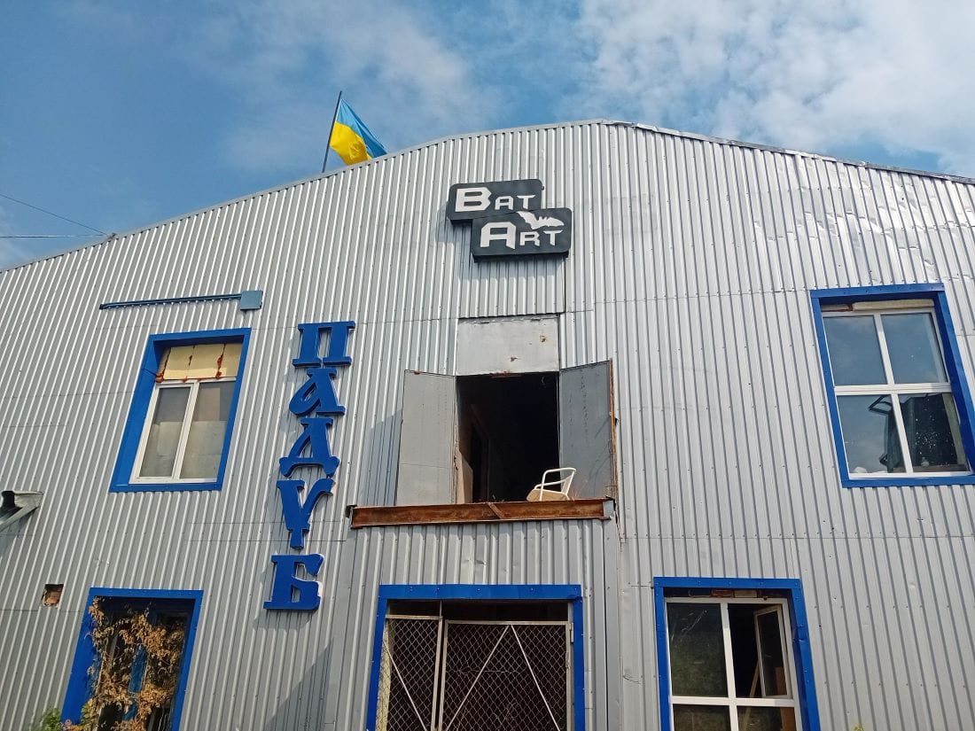

© Николета Атанасова
Във фабриката, сред грохота на няколкото машини, ветераните изработват най-специалните чаши, бутилки и ножове, които съм виждала. Във всяка чаша или нож има вграден куршум. Парите от продажбите отиват за бригадите, в които воюват.
Андрей Несмашни е доброволец в армията от първия ден на нахлуването на Русия в Украйна. По време на обстрелите на фабриката в Ирпин той воюва в Киевска област, а по-късно, в края на май 2022 г., го изпращат в Херсон. Там е ранен. През есента на 2022-ра се връща за лечение в Ирпин и започват да възстановят фабриката на Василий с идеята да я направят работно място за ветерани.
В момента тук работят десет мъже и една жена ветерани, но не се задържат много, защото, който се възстанови, веднага се връща на фронта като доброволец. Те имат право да останат в цивилния живот, но избират отново да воюват. Аз също на всеки два-три месеца се връщам на първа линия. Не може да е другояче. Въобще не си задавам въпроса да отида ли на фронта, или не, защото знам, че ако не го направя, ако всички не го правят, ние просто няма да сме живи. Украйна няма да я има като нация и страна. Аз не харесвам войната, не искам да има война, но трябва да отида и да се сражавам. Просто трябва. Това е моята страна, моята земя, аз обичам свободата и искам страната ми да е свободна.
Искам да ви кажа, че ние допускахме, че ще бъдем нападнати още през октомври 2021 г., и започнахме да се подготвяме за война, но Украйна беше лишена от оръжия и никой на Запад сякаш не вярваше истински, че Русия ще ни нападне. Затова и нямахме оръжия. Сега, почти три години по-късно, когато Русия завзема наши територии и оръжията не ни стигат, за да я защитим, Западът отново се чуди дали да ни даде оръжия, колко да са те, къде можем да ги използваме. Ще ви кажа. Нека само един от тези чиновници да отиде в Донбас например и да види за какво става дума на фронта. Да види как са въоръжени руснаците и как – ние. Да види десетките жертви, осакатените ни момчета и момичета и да прецени тази война има ли я наистина и колко е сериозна…
За съжаление, руското влияние и пропаганда пречат на трезвата оценка на ситуацията ни както на западните чиновници, така и на много украинци, преди да бъдем нападнати. Украинците обаче разбраха какво е руската пропаганда, когато Русия нахлу в територията ни и руснаците започнаха да избиват и изнасилват децата ни и майките ни. Всеки ден има обстрелван украински град и загиват невинни хора. Вие го виждате, защото сте тук, а къде са чиновниците от Европа и САЩ? Те ни казват от топлите си, безопасни местенца, че трябва да спазваме ограничения, за да използваме оръжията, които ни дават. Как ви се струва това? Никоя страна в Европа не е застрахована от руска агресия.
Знаете ли, аз дори не изпитвам гняв. Дори и да видя врага си в очите, не изпитвам нищо. Знам, че просто трябва да го убия, без никаква емоция. Емоциите и мислите пречат да си свършиш работата, защото това е професионалното – да не мислиш, а да действаш. Нямам съмнения, че съм прав в това, което върша, защото аз съм си вкъщи, в Украйна, а те са дошли тук и искат да ми я отнемат. Какво има да мисля? Това е. Просто война.
Андрей е сериозен, докато говори. Внезапно на лицето му се появява усмивка. Вече знам, че следва порция специфично украинско чувство за хумор. Не греша. Очите на Андрей се смеят малко цинично, все пак е дружелюбен. Когато проговаря, смехът му е и в гласа:
Някои си мислят, че войната е само да стреляш, но всъщност ти през цялото време копаеш. Много копаеш, постоянно копаеш, е, или тичаш…
Купуваме няколко чаши и си тръгваме от фабриката на Андрей с особено чувство. Украинците винаги те оставят без дъх заради историята, която са ти разказали, и в същото време се чувстваш нелепо, дори с въпросите, които си им задал. Идваш от спокойна страна и ги питаш за войната, в която живеят всеки ден. Как ли им изглеждаме отстрани, обяснявайки, че в собствената ни страна има хора, които не разбират какво прави Русия в Украйна. Сещам се какво ми каза Катя преди ден:
Те разказват своите истории, за да разберем каква цена плащат, за да сме ние с вас сега тук.

Ден по-късно вече сме в друг град, далеч от Ирпин. Олга с мъжа ѝ Андрей отварят вратата на подземие. Имам клаустрофобия и интуитивно спирам. Кучето им влиза първо, защото го прави всеки ден и знае, че вътре няма нищо страшно. Следвам го внимателно, докато Олга светва лампите.
Това е малката ни фабрика за дронове. Тук ги проектираме и конструираме. Имаме голям и няколко малки 3D принтера. След като сглобим всичко, отиваме на една поляна наблизо и ги пускаме да летят. Ако всичко е наред, произвеждаме цяла серия от съответния модел и ги изпращаме на фронта. Имаме различни, например този се казва „Хрущ“, или „Майски бръмбар“. Рамката му е изцяло наше производство. Той може да носи около три килограма полезен товар на разстояние около 35 километра. Сега сме го модифицирали за бойни условия срещу врага. Другият до него е изцяло боен дрон, реплика на китайския „Мавик“. Създадохме го тук, наше производство, по молба на военните. Нашият обаче стана по-добър, защото на него може да се постави произволна система за управление, а на китайския не е възможно. Нашият носи пет килограма и лети около 105 минути. Може да бъде бомбардировач, както и да доставя боеприпаси. Този тук е разузнавач с камери. А тези не са наше производство, подарък са ни, но военните ни ги изпратиха да ги ремонтираме. Наскоро ремонтирахме и руски, които нашите бяха пленили. Всъщност ние правим всичко в сферата на дроновете, от което военните имат нужда, включително и тези безпилотни самолети, които имат различни приложения, в зависимост с какво ще ги комплектувате. Предимството им е, че може много лесно да се сглобяват и разглобяват. Този конкретно е разузнавач.

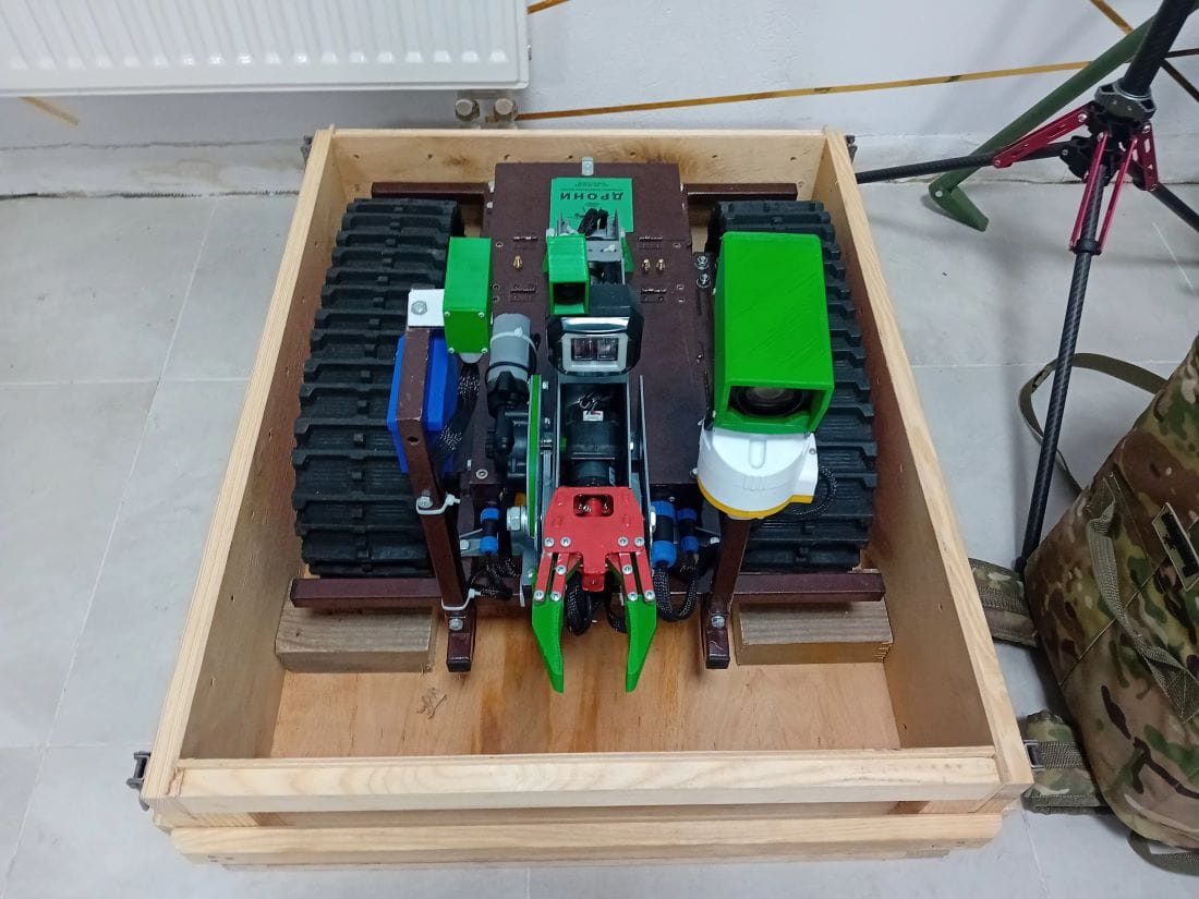
© Николета Атанасова
Докато Андрей говори, не спира да ходи из голямата стая, размахва ръце като възторжен диригент и постоянно взема в ръце един или друг дрон, после ги оставя и започва да сглобява безпилотния самолет. Говори за тях с огромна усмивка, в погледа му има гордост и радост от това, което прави.
Андрей е инженер и е работил за големи компании, които произвеждат дронове, още преди началото на войната. След нахлуването на Русия в Украйна той и Олга създават своята фабрика за дронове.
Разбрахме, че през големите фирми трудно ще бъдем полезни на нашите момчета на фронта, защото е много бавно, дори невъзможно да прокараш своя разработка в големите компании, а тук, в нашата собствена фабрика, ние правим това, от което имат нужда на фронта. Обаждат се и ни казват: трябва ни това и това, да може да прави тези и тези неща, и ние модифицираме и разработваме всичко веднага сами според конкретните нужди на фронта днес, а не отпреди няколко месеца. Това е много важно, защото войната се променя всеки ден, условията и нуждите на войниците – също. Ние сме в пряк контакт с тях и сме достатъчно гъвкави, за да правим това, което им трябва в момента. В голяма компания това не може да стане.
Щастливи сме, че с нашите дронове спасяваме живота на нашите войници, защото много често дроновете успяват да заменят пехотинците. Например за обучението на един пилот на вертолет са нужни няколко години, самата машина струва милиони долари и накрая врагът сваля вертолета, пилотът загива или отива в плен. Това е огромна загуба. При дроновете, дори и да бъде свалено устройството, пилотът му седи на сигурно място в тила и загубата е само малко труд и пари. Какво е тази загуба, ако спаси дори един човешки живот?! Дронове се правят на килограм, но хората… Войната вече е война на дронове. Само трябва добре да се обучават пилоти, това става за около месец-два. Засега не достигат нито пилотите, нито обучаващите, но е въпрос на време. Ние правим постоянно обучения за нашите продукти. Елате да видите – това сме произвели от сутринта, само за няколко часа.
© Николета Атанасова
Андрей ме води в съседната стая. Там около масите седят няколко човека. Един запоява, друг прави тестове на компютър, трети сглобява частите на дрон. Съсредоточени са, дори не ни поглеждат. В различни райони на Украйна има няколко клона на фабриката на Андрей и за него работят около трийсет човека. Не искам да нарушавам спокойствието в тясната, задръстена с части стаичка и набързо разглеждам наоколо, но Андрей ме кара да клекнем до малки 3D принтери, за видя как става магията…
© Николета Атанасова
Тръгваме си зашеметени от подземието, в което се крие царството на бъдещето. Андрей и Олга ни махат на входа с усмивка. В таксито, което ни кара към града, разглеждам няколкото снимки, които съм направила, и си мисля за магията… Телефонът ми звъни в едно от приложенията. Мой познат ме пита развълнувано: „Търсих те няколко пъти, не дава заето, но какво ми говори украинският оператор?“ Усмихвам се и кратичко отговарям:
Моля, изчакайте! Абонатът говори за победата.
На второ четене: „Спомен за гората“
Post Syndicated from original https://www.toest.bg/na-vtoro-chetene-spomen-za-gorata/
„Спомен за гората“ от Дамир Каракаш

превод от хърватски Русанка Ляпова, София: изд. ICU, 2023
Клише е, но не е лъжа – в малките книги има една особена големина. Не равностойна на мащабност и епичност, а измерима като разрастване навътре. „Спомен за гората“ е точно такава книжка (в нежния смисъл на това умалително). Тази проза напълно се вписва в профила на своите издатели от ICU, които публикуват на български и словенеца Горан Войнович.
Дамир Каракаш е хърватин, един от водещите писатели в страната си, но засега това е първата му и единствена книга на български. Не знам дали изборът точно на този автобиографичен роман, а не на някой от по-мащабните или известните му е продиктуван от други съображения (например финансиране), но със сигурност това му произведение, почти повест, отвори апетита ми за още от прозата на автора.
Каракаш е роден в село в Лика, планинския район на страната, и – наред с други „по-сериозни“ неща – е учил и агрономия – съвсем тематично за автор, толкова обвързан със селския живот и земята, както е в тази книга. Изглежда, че и в други свои романи той проблематизира сблъсъка между селския произход и градската среда. При това за Каракаш се казва, че е от малцината автори, които пишат за своята Лика, използвайки тамошния диалект. Други негови романи пък описват живота му в Париж („Прекрасно място за нещастие“) или се занимават с представителите на загребската субкултура по време на войната в Югославия (Blue Moon).
„Спомен за гората“ е носталгичен разказ за детството и израстването на село през 60-те –
ту земен, жив и натуралистичен до графичност на езика, ту лиричен и чувствителен, ту почти комичен. Гората е символичната рамка на този живот в оазиса на опитоменото от човека пространство – тя е място за излаз на детското въображение, уютна възможност за отдалечаване от дома, но и място друго, застрашително, в което броди една от метафорите на романа – голямата и страшна мечка, разкъсваща хора. Място на търсене и изпитания и в крайна сметка – на инициация за порасналия герой.
Героят, разбира се, е алтер егото на Дамир Каракаш – момче, страдащо от слабо, болно сърце. Факт, който в тази сурова, лишена от префиненост и „лигавщини“ среда, където най-важното е да се утвърдиш като мъж, ще се окаже проблемен. Неслучайно най-голямото опасение на героя е да го преценят като недостоен да влезе в казармата, а най-голямата му мечта – да стане военен. Заради желанието да възмъжее момчето ще подложи себе си на режим, който ще застраши здравето и дори живота му. В този контекст отношението на близките се лута между смута от грубоватото му жалене („Де ще се дене клетият, такъв недъгав?“, „Що ги създава Господ такива, негодни за живот?“) и порива да омаловажат слабостта му в името на вярата, че за да се кали и да бъде като всички останали, той не бива да бъде щаден.
Книгата е организирана в глави, които са привидно несвързани, макар между тях да има някаква – най-малкото хронологична – връзка: от детството, през неусетното порастване, до юношеството. Всяка е сцена сама по себе си, като особено ми допадна предизвикателството към читателските очаквания. Защото главите не следват сюжетните необходимости и често завършват без изненади, без кулминации и драма. Просто става онова, което се случва в ежедневния живот. Да, невинаги в него има обрати, напрежение преди добрия завършек, та дори понякога да си казваме „Е, и?“. Каквото и да се случва тук, дори да е нелеко и различно от ежедневния битов ритъм, то е обгърнато в някакво усещане за естественост, за познатост, дори за покой.
Каракаш не е търсил изключителното, откроената събитийност – напротив, наративът е изграден от „баналности“ (в хубавия, познат смисъл на тази дума), от битовизми, които ни се струват толкова близки и познати в един балкански контекст. Ето например едно „събитие“ – баща му донася първата в селото тоалетна тип „клекало“ и първия допотопен душ, като, разбира се, е страшно горд от това („Да се види кой е пръв в селото“). За разлика от това, другите, големите събития на историческия контекст присъстват изключително фоново, дискретно, на практика незабележимо.
Романът на Дамир Каракаш ни връща към осъзнаването, че добрата литература може да е направена от житейските незначителности.
От важните извън нея битови всекидневности. Игрите, първите цигари и мастурбации; пасенето на добитъка и работата на полето; дочуването на прибързаното съвкупление на родителите в тясната къща; типичното безцеремонно отношение към животните на село; страхопочитанието пред първия телевизор; неизбежните псувни; коленето на прасето; ценността и на най-малките притежания по времето на соца; толкова естествената липса на гузност да се сдобиеш с тях по коварен начин; местните „лоши момчета“; лова с баща ти; дъжда или жегата; човешките нечистотии; тайната болка по възрастен съсед, който приживе е бил твое убежище; и да, грубите, натурални емоции…
… най-неочаквано тя [майка ми] ме целуна по бузата, а аз се стреснах, защото не съм свикнал. Баща ми и майка ми никога не ме целуват, само се ръкуват с мен. Не ме целуват даже за рождения ми ден, защото никога не го празнувам. У нас на село не съм виждал някой да целуне някого. А баща си не съм го виждал и да плаче; даже не мога да си го представя.
Не обичам клишето „тиха книга“, но тази е точно такава, при цялата си фина живост. Разказ, в който въображението надскача уредения бит, за да навлезе в гората – там, където дебне стръвницата, символ на болестта, на опасността, но и въобще на предстоящото. Всяко порастване – всяко живеене – е дебненето за тази мечка. И срещата е неизбежна.

„Спомен за гората“ е и от тези книги, които задължително ти напомнят за други подобни. Нима не сме чели десетки романи за същите онези неща, които правят всички на тази възраст, дори и отвъд конкретното поколение? Тайната се крие именно в това дежавю, в тази уютна познатост. Мисля си тук за прекрасната и много подобна автофикционална книга на Юли Шумарев „Макгахански блусове и балади“ (за детството с родителите му, баба му и дядо му на един от пловдивските сокаци през 70-те); за „Когато големите станат малки“ от Алберт Бенбасат (за детството му и еврейското му семейство в стара София от 50-те); за „Струни“ на Радко Пенев; за първата част от трилогията на Иван Станков (детството през 60-те покрай Дунава); за „Цялото наше безумство“ на малайската авторка Ши-Ли Коу (да, звучи далечно, но е точно като при нас!) и за още много други книги. Всички те си струват да бъдат прочетени, също като тази.
Активните дарители на „Тоест“ получават постоянна отстъпка в размер нa 20% от коричната цена на всички заглавия от каталога на издателство ICU, както и на няколко други български издателства в рамките на партньорската програма Читателски клуб „Тоест“. За повече информация прочетете на toest.bg/club.
Никой от нас не чете единствено най-новите книги. Тогава защо само за тях се пише? „На второ четене“ е рубрика, в която отваряме списъците с книги, публикувани преди поне година, четем ги и препоръчваме любимите си от тях. Рубриката е част от партньорската програма Читателски клуб „Тоест“. Изборът на заглавия обаче е единствено на авторите – Стефан Иванов и Антония Апостолова, които биха ви препоръчали тези книги и ако имаше как веднъж на две седмици да се разходите с тях в книжарницата.
Hannah Shaw & Andrew Marttila | Cats of the World | Talks at Google
Post Syndicated from Talks at Google original https://www.youtube.com/watch?v=iFrcKLKZ-OI
Security updates for Monday
Post Syndicated from jake original https://lwn.net/Articles/994080/
Security updates have been issued by Debian (docker.io, libreoffice, node-dompurify, python-reportlab, and thunderbird), Fedora (buildah, chromium, kernel, kernel-headers, libgsf, mosquitto, p7zip, podman, python-cramjam, python-virtualenv, redis, rust-async-compression, rust-brotli, rust-brotli-decompressor, rust-libcramjam, rust-libcramjam0.2, rust-nu-command, rust-nu-protocol, rust-redlib, rust-tower-http, thunderbird, and webkit2gtk4.0), Oracle (.NET 6.0, .NET 8.0, e2fsprogs, firefox, golang, openssl, python3-setuptools, systemd, and thunderbird), SUSE (chromium, firefox, java-jwt, libmozjs-128-0, libwireshark18, ntpd-rs, OpenIPMI, thunderbird, and wireshark), and Ubuntu (firefox, python2.7, python3.5, thunderbird, and ubuntu-advantage-desktop-daemon).
Motorcade Mishap: 1975 Presidential Limousine Accident
Post Syndicated from The History Guy: History Deserves to Be Remembered original https://www.youtube.com/watch?v=pNRLPzoQhA4
Perfectl Malware
Post Syndicated from Bruce Schneier original https://www.schneier.com/blog/archives/2024/10/perfectl-malware.html
Perfectl in an impressive piece of malware:
The malware has been circulating since at least 2021. It gets installed by exploiting more than 20,000 common misconfigurations, a capability that may make millions of machines connected to the Internet potential targets, researchers from Aqua Security said. It can also exploit CVE-2023-33246, a vulnerability with a severity rating of 10 out of 10 that was patched last year in Apache RocketMQ, a messaging and streaming platform that’s found on many Linux machines.
The researchers are calling the malware Perfctl, the name of a malicious component that surreptitiously mines cryptocurrency. The unknown developers of the malware gave the process a name that combines the perf Linux monitoring tool and ctl, an abbreviation commonly used with command line tools. A signature characteristic of Perfctl is its use of process and file names that are identical or similar to those commonly found in Linux environments. The naming convention is one of the many ways the malware attempts to escape notice of infected users.
Perfctl further cloaks itself using a host of other tricks. One is that it installs many of its components as rootkits, a special class of malware that hides its presence from the operating system and administrative tools. Other stealth mechanisms include:
- Stopping activities that are easy to detect when a new user logs in
- Using a Unix socket over TOR for external communications
- Deleting its installation binary after execution and running as a background service thereafter
- Manipulating the Linux process pcap_loop through a technique known as hooking to prevent admin tools from recording the malicious traffic
- Suppressing mesg errors to avoid any visible warnings during execution.
The malware is designed to ensure persistence, meaning the ability to remain on the infected machine after reboots or attempts to delete core components. Two such techniques are (1) modifying the ~/.profile script, which sets up the environment during user login so the malware loads ahead of legitimate workloads expected to run on the server and (2) copying itself from memory to multiple disk locations. The hooking of pcap_loop can also provide persistence by allowing malicious activities to continue even after primary payloads are detected and removed.
Besides using the machine resources to mine cryptocurrency, Perfctl also turns the machine into a profit-making proxy that paying customers use to relay their Internet traffic. Aqua Security researchers have also observed the malware serving as a backdoor to install other families of malware.
Something this complex and impressive implies that a government is behind this. North Korea is the government we know that hacks cryptocurrency in order to fund its operations. But this feels too complex for that. I have no idea how to attribute this.