Recommender systems have become essential components of digital services across e-commerce, streaming media, and social networks [1, 2]. At Netflix, these systems drive significant product and business impact by connecting members with relevant content at the right time [3, 4]. While our recommendation foundation model (FM) has made substantial progress in understanding user preferences through large-scale learning from interaction histories (please refer to this article about FM @ Netflix), there is an opportunity to further enhance its capabilities. By extending FM to incorporate the prediction of underlying user intents, we aim to enrich its understanding of user sessions beyond next-item prediction, thereby offering a more comprehensive and nuanced recommendation experience.
Recent research has highlighted the importance of understanding user intent in online platforms [5, 6, 7, 8]. As Xia et al. [8] demonstrated at Pinterest, predicting a user’s future intent can lead to more accurate and personalized recommendations. However, existing intent prediction approaches typically employ simple multi-task learning that adds intent prediction heads to next-item prediction models without establishing a hierarchical relationship between these tasks.
To address these limitations, we introduce FM-Intent, a novel recommendation model that enhances our foundation model through hierarchical multi-task learning. FM-Intent captures a user’s latent session intent using both short-term and long-term implicit signals as proxies, then leverages this intent prediction to improve next-item recommendations. Unlike conventional approaches, FM-Intent establishes a clear hierarchy where intent predictions directly inform item recommendations, creating a more coherent and effective recommendation pipeline.
FM-Intent makes three key contributions:
A novel recommendation model that captures user intent on the Netflix platform and enhances next-item prediction using this intent information.
A hierarchical multi-task learning approach that effectively models both short-term and long-term user interests.
Comprehensive experimental validation showing significant performance improvements over state-of-the-art models, including our foundation model.
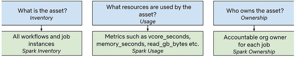
Understanding User Intent in Netflix
In the Netflix ecosystem, user intent manifests through various interaction metadata, as illustrated in Figure 1. FM-Intent leverages these implicit signals to predict both user intent and next-item recommendations.
Figure 1: Overview of user engagement data in Netflix. User intent can be associated with several interaction metadata. We leverage various implicit signals to predict user intent and next-item.
In Netflix, there can be multiple types of user intents. For instance,
Action Type: Categories reflecting what users intend to do on Netflix, such as discovering new content versus continuing previously started content. For example, when a member plays a follow-up episode of something they were already watching, this can be categorized as “continue watching” intent.
Genre Preference: The pre-defined genre labels (e.g., Action, Thriller, Comedy) that indicate a user’s content preferences during a session. These preferences can shift significantly between sessions, even for the same user.
Movie/Show Type: Whether a user is looking for a movie (typically a single, longer viewing experience) or a TV show (potentially multiple episodes of shorter duration).
Time-since-release: Whether the user prefers newly released content, recent content (e.g., between a week and a month), or evergreen catalog titles.
These dimensions serve as proxies for the latent user intent, which is often not directly observable but crucial for providing relevant recommendations.
FM-Intent Model Architecture
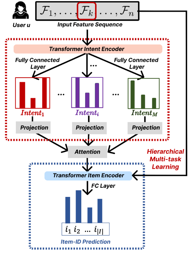
FM-Intent employs a hierarchical multi-task learning approach with three major components, as illustrated in Figure 2.
Figure 2: An architectural illustration of our hierarchical multi-task learning model FM-Intent for user intent and item predictions. We use ground-truth intent and item-ID labels to optimize predictions.
1. Input Feature Sequence Formation
The first component constructs rich input features by combining interaction metadata. The input feature for each interaction combines categorical embeddings and numerical features, creating a comprehensive representation of user behavior.
2. User Intent Prediction
The intent prediction component processes the input feature sequence through a Transformer encoder and generates predictions for multiple intent signals.
The Transformer encoder effectively models the long-term interest of users through multi-head attention mechanisms. For each prediction task, the intent encoding is transformed into prediction scores via fully-connected layers.
A key innovation in FM-Intent is the attention-based aggregation of individual intent predictions. This approach generates a comprehensive intent embedding that captures the relative importance of different intent signals for each user, providing valuable insights for personalization and explanation.
3. Next-Item Prediction with Hierarchical Multi-Task Learning
The final component combines the input features with the user intent embedding to make more accurate next-item recommendations.
FM-Intent employs hierarchical multi-task learning where intent predictions are conducted first, and their results are used as input features for the next-item prediction task. This hierarchical relationship ensures that the next-item recommendations are informed by the predicted user intent, creating a more coherent and effective recommendation model.
Offline Results
We conducted comprehensive offline experiments on sampled Netflix user engagement data to evaluate FM-Intent’s performance. Note that FM-Intent uses a much smaller dataset for training compared to the FM production model due to its complex hierarchical prediction architecture.
Next-Item and Next-Intent Prediction Accuracy
Table 1 compares FM-Intent with several state-of-the-art sequential recommendation models, including our production model (FM-Intent-V0).
Table 1: Next-item and next-intent prediction results of baselines and our proposed method FM-Intent on the Netflix user engagement dataset.
All metrics are represented as relative % improvements compared to the SOTA baseline: TransAct. N/A indicates that a model is not capable of predicting a certain intent. Note that we added additional fully-connected layers to LSTM, GRU, and Transformer baselines in order to predict user intent, while we used original implementations for other baselines. FM-Intent demonstrates statistically significant improvement of 7.4% in next-item prediction accuracy compared to the best baseline (TransAct).
Most baseline models show limited performance as they either cannot predict user intent or cannot incorporate intent predictions into next-item recommendations. Our production model (FM-Intent-V0) performs well but lacks the ability to predict and leverage user intent. Note that FM-Intent-V0 is trained with a smaller dataset for a fair comparison with other models; the actual production model is trained with a much larger dataset.
Qualitative Analysis: User Clustering
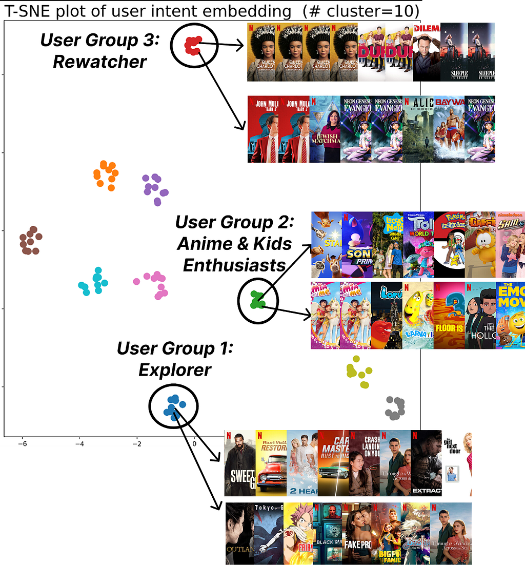
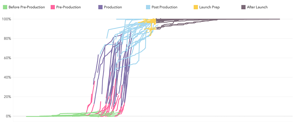
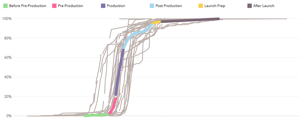
Figure 3: K-means++ (K=10) clustering of user intent embeddings found by FM-Intent; FM-Intent finds unique clusters of users that share the similar intent.
FM-Intent generates meaningful user intent embeddings that can be used for clustering users with similar intents. Figure 3 visualizes 10 distinct clusters identified through K-means++ clustering.These clusters reveal meaningful user segments with distinct viewing patterns:
Users who primarily discover new content versus those who continue watching recent/favorite content.
Users with specific viewing patterns (e.g., Rewatchers versus casual viewers).
Potential Applications of FM-Intent
FM-Intent has been successfully integrated into Netflix’s recommendation ecosystem, can be leveraged for several downstream applications:
Personalized UI Optimization: The predicted user intent could inform the layout and content selection on the Netflix homepage, emphasizing different rows based on whether users are in discovery mode, continue-watching mode, or exploring specific genres.
Analytics and User Understanding: Intent embeddings and clusters provide valuable insights into viewing patterns and preferences, informing content acquisition and production decisions.
Enhanced Recommendation Signals: Intent predictions serve as features for other recommendation models, improving their accuracy and relevance.
Search Optimization: Real-time intent predictions help prioritize search results based on the user’s current session intent.
Conclusion
FM-Intent represents an advancement in Netflix’s recommendation capabilities by enhancing them with hierarchical multi-task learning for user intent prediction. Our comprehensive experiments demonstrate that FM-Intent significantly outperforms state-of-the-art models, including our prior foundation model that focused solely on next-item prediction. By understanding not just what users might watch next but what underlying intents users have, we can provide more personalized, relevant, and satisfying recommendations.
Acknowledgements
We thank our stunning colleagues in the Foundation Model team & AIMS org. for their valuable feedback and discussions. We also thank our partner teams for getting this up and running in production.
References
[1] Amatriain, X., & Basilico, J. (2015). Recommender systems in industry: A netflix case study. In Recommender systems handbook (pp. 385–419). Springer.
[2] Gomez-Uribe, C. A., & Hunt, N. (2015). The netflix recommender system: Algorithms, business value, and innovation. ACM Transactions on Management Information Systems (TMIS), 6(4), 1–19.
[3] Jannach, D., & Jugovac, M. (2019). Measuring the business value of recommender systems. ACM Transactions on Management Information Systems (TMIS), 10(4), 1–23.
[4] Bhattacharya, M., & Lamkhede, S. (2022). Augmenting Netflix Search with In-Session Adapted Recommendations. In Proceedings of the 16th ACM Conference on Recommender Systems (pp. 542–545).
[5] Chen, Y., Liu, Z., Li, J., McAuley, J., & Xiong, C. (2022). Intent contrastive learning for sequential recommendation. In Proceedings of the ACM Web Conference 2022 (pp. 2172–2182).
[6] Ding, Y., Ma, Y., Wong, W. K., & Chua, T. S. (2021). Modeling instant user intent and content-level transition for sequential fashion recommendation. IEEE Transactions on Multimedia, 24, 2687–2700.
[7] Liu, Z., Chen, H., Sun, F., Xie, X., Gao, J., Ding, B., & Shen, Y. (2021). Intent preference decoupling for user representation on online recommender system. In Proceedings of the Twenty-Ninth International Conference on International Joint Conferences on Artificial Intelligence (pp. 2575–2582).
[8] Xia, X., Eksombatchai, P., Pancha, N., Badani, D. D., Wang, P. W., Gu, N., Joshi, S. V., Farahpour, N., Zhang, Z., & Zhai, A. (2023). TransAct: Transformer-based Realtime User Action Model for Recommendation at Pinterest. In Proceedings of the 29th ACM SIGKDD Conference on Knowledge Discovery and Data Mining (pp. 5249–5259).
In a digital advertising platform, a robust feedback system is essential for the lifecycle and success of an ad campaign. This system comprises of diverse sub-systems designed to monitor, measure, and optimize ad campaigns. At Netflix, we embarked on a journey to build a robust event processing platform that not only meets the current demands but also scales for future needs. This blog post delves into the architectural evolution and technical decisions that underpin our Ads event processing pipeline.
Ad serving acts like the “brain” — making decisions, optimizing delivery and ensuring right Ad is shown to the right member at the right time. Meanwhile, ad events, after an Ad is rendered, function like “heartbeats”, continuously providing real-time feedback (oxygen/nutrients) that fuels better decision-making, optimizations, reporting, measurement, and billing. Expanding on this analogy:
Just as the brain relies on continuous blood flow, ad serving depends on a steady stream of ad events to adjust next ad serving decision, frequency capping, pacing, and personalization.
If the nervous system stops sending signals (ad events stop flowing), the brain (ad serving) lacks critical insights and starts making poor decisions or even fails.
The healthier and more accurate the event stream (just like strong heart function), the better the ad serving system can adapt, optimize, and drive business outcomes.
Let’s dive into the journey of building this pipeline.
The Pilot
In November 2022, we launched a brand new basic ads plan, in partnership with Microsoft. The software systems extended the existing Netflix playback systems to play ads. Initially, the system was designed to be simple, secure, and efficient, with an underlying ethos of device-originated and server-proxied operations. The system consisted of three main components: the Microsoft Ad Server, Netflix Ads Manager, and Ad Event Handler. Each ad served required tracking to ensure the feedback loop functioned effectively, providing the external ad server with insights on impressions, frequency capping (advertiser policy that limits the number of times a user sees a specific ad), and monetization processes.
Key features of this system include:
Client Request: Client devices request for ads during an ad break from Netflix playback systems, which is then decorated with information by ads manager to request ads from the ad server.
Server-Side Ad Insertion: The Ad Server sends ad responses using the VAST (Video Ad Serving Template) format.
Netflix Ads Manager: This service parses VAST documents, extracts tracking event information, and creates a simplified response structure for Netflix playback systems and client devices. — The tracking information is packed into a structured protobuf data model. — This structure is encrypted to create an opaque token. — The final response, informs the client devices, when to send an event and the corresponding token.
Client Device: During ad playback, client devices send events accompanied by a token. The Netflix telemetry system then enqueues all these events in Kafka for asynchronous processing.
Ads Event Handler: This component is a Kafka consumer, that reads/decrypts the event payload and forwards the tracking information encoded back to the ad server and other vendors.
Fig 1: Basic Ad Event Handling System
There is an excellent prior blog post that explains how this systems was tested end-to-end at scale. This system design allowed us to quickly add new integrations for verification with vendors like DV, IAS and Nielsen for measurement.
The Expansion
As we continued to expand our third-party (3P) advertising vendors for measurement, tracking and verification, we identified a critical trend: growth in the volume of data encapsulated within opaque tokens. These tokens, which are cached on client devices, present a risk of elevated memory usage, potentially impacting device performance. We also anticipated increase in third-party tracking URLs, metadata needs, and more event types as our business added new capabilities.
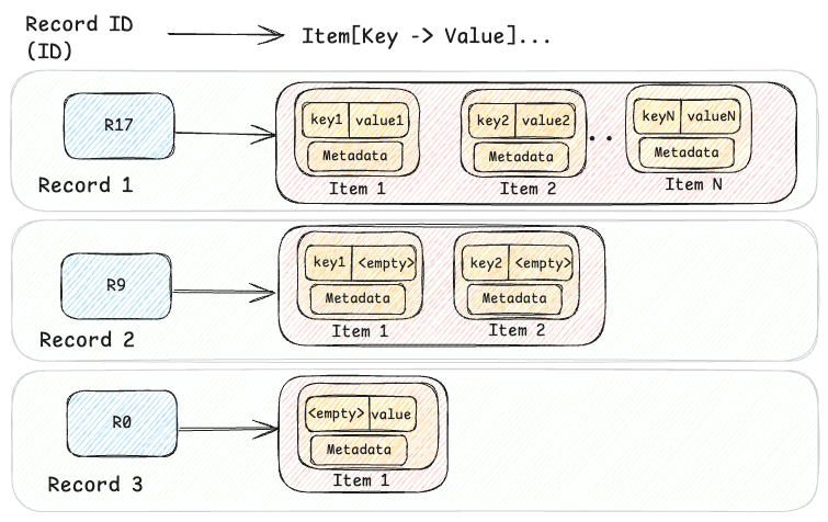
To strategically address these challenges, we introduced a new persistence layer using Key-Value abstraction, between ad serving and event handling system: Ads Metadata Registry. This transient storage service stores metadata for each Ad served, and upon callback, event handler would read the tracking information to relay information to the vendors. The contract between the client device and Ads systems continues to use the opaque token per event, but now, instead of tracking information, it contains reference identifiers — Ad ID, the corresponding metadata record ID in the registry and the event name. This approach future proofed our systems to handle any growth in data that needs to pass from ad serving to event handling systems.
Fig 2: Storage service between Ad Serving & Reporting
The Evolution
In January of 2024, we decided to invest in in-house advertising technology platform. This implied that the event processing pipeline had to evolve significantly — attain parity with existing offerings and continue to support new product launches with rapid iterations using in-house Netflix Ad Server. This required re-evaluation of the entire architecture across all of Ads engineering teams.
First, we made an inventory of the use-cases that would need to be supported through ad events.
We’d need to start supporting frequency capping in-house for all ads through Netflix Ad server.
Incorporate pricing information for impressions to set the stage for billing events, which are used to charge advertisers.
A robust reporting system to share campaign reports with advertisers, combined with metrics data collection, helps assess the delivery and effectiveness of the campaign.
Scale event handler to perform tracking information look-ups across different vendors.
Next, we examined upcoming launches, such as Pause/Display ads, to gain deeper insights into our strategic initiatives. We recognized that Display Ads would utilize a distinct logging framework, suggesting that different upstream pipelines might deliver ad telemetry. However, the downstream use-cases were expected to remain largely consistent. Additionally, by reviewing the goals of our telemetry teams, we saw large initiatives aimed at upgrading the platform, indicating potential future migrations.
Keeping the above insights & challenges in mind,
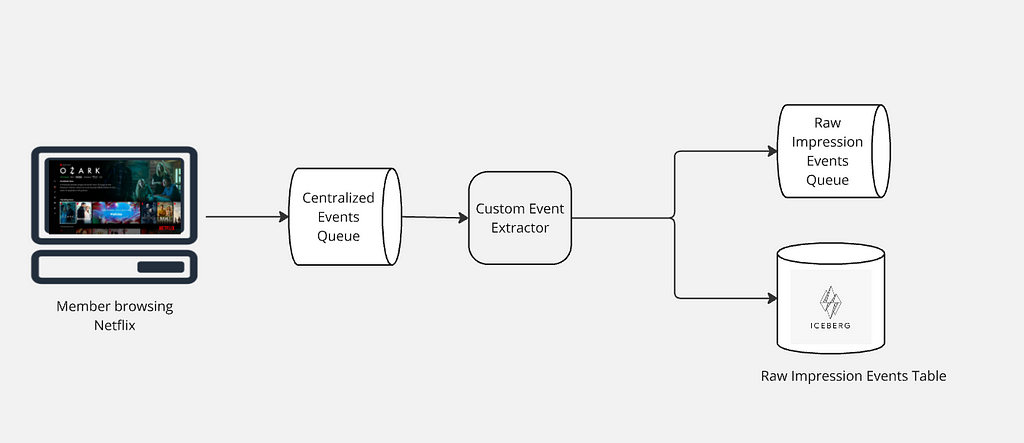
We planned a centralized ad event collection system. This centralized service would consolidate common operations like decryption of tokens, enrichment, hashing identifiers into a single step execution and provide a single unified data contract to consumers that is highly extensible (like being agnostic to ad server & ad media).
We proposed moving all consumers of ad telemetry downstream of the centralized service. This creates a clean separation between upstream systems and consumers in Ads Engineering.
In the initial development phase of our advertising system, a crucial component was the creation of ad sessions based on individual ad events. This system was constructed using ad playback telemetry, which allowed us to gather essential metrics from these ad sessions. A significant decision in this plan was to position the ad sessionization process downstream of the raw ad events.
The proposal also recommended moving all our Ads data processing pipelines for reporting/analytics/metrics for Ads using the data published by the centralized system.
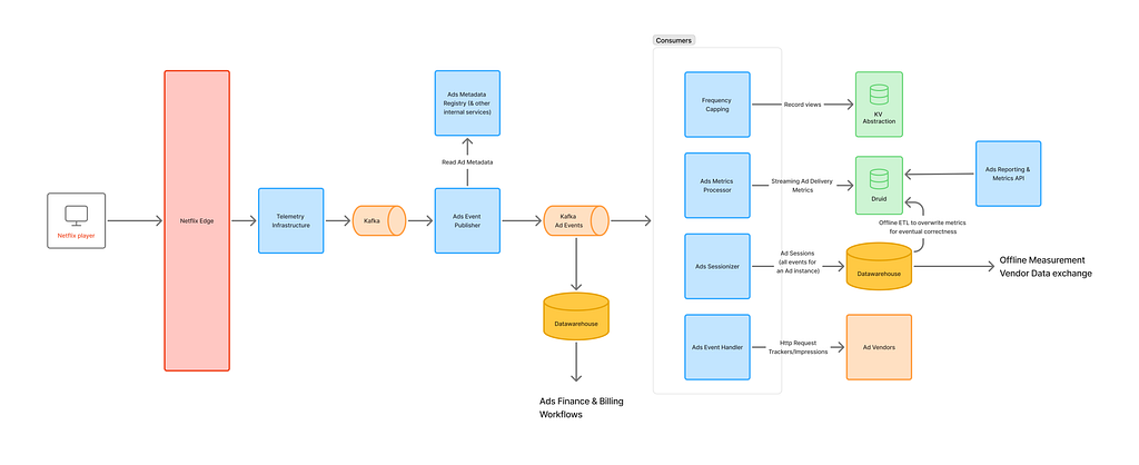
Putting together all the components in our vision –
Fig 3: Ad Event processing pipeline
Key components on event processing pipeline –
Ads Event Publisher: This centralized system is responsible for collecting ads telemetry and providing unified ad events to the ads engineering teams. It supports various functions such as measurement, finance/billing, reporting, frequency capping, and maintaining an essential feedback loop back to the ad server.
Realtime Consumers
Frequency Capping: This system tracks impressions for each campaign, profile, and any other frequency capping parameters set up for the campaign. It is utilized by the Ad Server during each ad decision to ensure ads are served with frequency limits.
Ads Metrics: This component is a Flink job that transforms raw data to a set of dimensions and metrics, subsequently writing to Apache Druid OLAP database. The streaming data is further backed by an offline process that corrects any inaccuracy during streaming ingestion and providing accurate metrics. It provides real-time metrics to assess the delivery health of campaigns and applies budget capping functionality.
Ads Sessionizer: An Apache Flink job that consolidates all events related to a single ad into an Ad Session. This session provides real-time information about ad playback, offering essential business insights and reporting. It is a crucial job that supports all downstream analytical and reporting processes.
Ads Event Handler: This service continuously sends information to ad vendors by reading tracking information from ad events, ensuring accurate and timely data exchange.
Billing/Revenue: These are offline workflows designed to curate impressions, supporting billing and revenue recognition processes.
Ads Reporting & Metrics: This service powers reporting module for our account managers and provides a centralized metrics API that help assess the delivery of a campaign.
This was a massive multi-quarter effort across different engineering teams. With extensive planning (kudos to our TPM team!) and coordination, we were able to iterate fast, build several services and execute the vision above, to power our in-house ads technology platform.
Conclusion
These systems have significantly accelerated our ability to launch new capabilities for the business.
Through our partnership with Microsoft, Display Ad events were integrated into the new pipeline for reusability and ensuring when launching through Netflix ads systems, all use-cases were covered.
Programmatic buying capabilities now support the exchange of numerous trackers and dynamic bid prices on impression events.
Sharing opt-out signals helps ensure privacy and compliance with GDPR regulations for Ads business in Europe, supporting accurate reporting and measurement.
New event types like Ad clicks and scanning of QR codes events also flow through the pipeline, ensuring all metrics and reporting are tracked consistently.
Key Takeways
Strategic, incremental evolution: The development of our ads event processing systems has been a carefully orchestrated journey. Each iteration was meticulously planned by addressing existing challenges, anticipating future needs, and showcasing teamwork, planning, and coordination across various teams. These pillars have been fundamental to the success of this journey.
Data contract: A clear data contract has been pivotal in ensuring consistency in interpretation and interoperability across our systems. By standardizing the data models, and establishing a clear data exchange between ad serving, and centralized event collection, our teams have been able to iterate at exceptional speed and continue to deliver many launches on time.
Separation of concerns: Consumers are relieved from the need to understand each source of ad telemetry or manage updates and migrations. Instead, a centralized system handles these tasks, allowing consumers to focus on their core business logic.
We have an exciting list of projects on the horizon. These include managing ad events from ads on Netflix live streams, de-duplication processes, and enriching data signals to deliver enhanced reporting and insights. Additionally, we are advancing our Native Ads strategy, integrating Conversion API for improved conversion tracking, among many others.
This is definitely not a season finale; it’s just the beginning of our journey to create a best-in-class ads technology platform. We warmly invite you to share your thoughts and comments with us. If you’re interested in learning more or becoming a part of this innovative journey, Ads Engineering is hiring!
At Netflix, delivering the best possible experience for our members is at the heart of everything we do, and we know we can’t do it alone. That’s why we work closely with a diverse ecosystem of technology partners, combining their deep expertise with our creative and operational insights. Together, we explore new ideas, develop practical tools, and push technical boundaries in service of storytelling. This collaboration not only empowers the talented creatives working on our shows with better tools to bring their vision to life, but also helps us innovate in service of our members. By building these partnerships on trust, transparency, and shared purpose, we’re able to move faster and more meaningfully, always with the goal of making our stories more immersive, accessible, and enjoyable for audiences everywhere. One area where this collaboration is making a meaningful impact is in improving dialogue intelligibility, from set to screen. We call this the Dialogue Integrity Pipeline.
Dialogue Integrity Pipeline
We’ve all been there, settling in for a night of entertainment, only to find ourselves straining to catch what was just said on screen. You’re wrapped up in the story, totally invested, when suddenly a key line of dialogue vanishes into thin air. “Wait, what did they say? I can’t understand the dialogue! What just happened?”
You may pick up the remote and rewind, turn up the volume, or try to stay with it and hope this doesn’t happen again. Creating sophisticated, modern series and films requires an incredible artistic & technical effort. At Netflix, we strive to ensure those great stories are easy for the audience to enjoy. Dialogue intelligibility can break down at multiple points in what we call the Dialogue Integrity Pipeline, the journey from on-set capture to final playback at home. Many facets of the process can contribute to dialogue that’s difficult to understand:
Naturalistic acting styles, diverse speech patterns, and accents
Noisy locations, microphone placement problems on set
Audio compromises through the distribution pipeline
TVs with inadequate speakers, noisy home environments
Addressing these issues is critical to maintaining the standard of excellence our content deserves.
Measurement at Scale
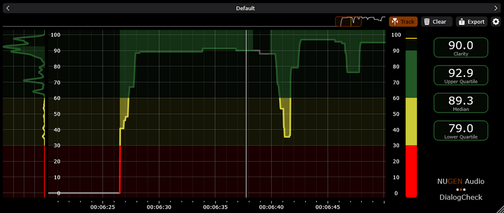
Netflix utilizes industry-standard loudness meters to measure content and its adherence to our core loudness specifications. This tool also provides feedback on audio dynamic range (loud to soft) which impacts dialogue intelligibility. The Audio Algorithms team at Netflix wanted to take these measurements further and develop a holistic understanding of dialogue intelligibility throughout the runtime of a given title.
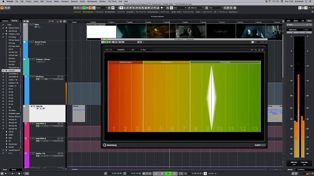
The team developed a Speech Intelligibility measurement system based on the Short-time Objective Intelligibility (STOI) metric [Taal et al. (IEEE Transactions on Audio, Speech, and Language Processing)]. Firstly, a speech activity detector analyses the dialogue stem to render speech utterances, which are then compared to non-speech sounds in the mix, typically Music and Effects. Then the system calculates the Signal-to-Noise ratio, in each speech frequency band, the results of which are summarized succinctly, per-utterance on the range [0, 1.0], to quantify the degree to which competing Music and Effects can distract the listener.
This chart shows how eSTOI (extended Short-Time Objective Intelligibility) method measures dialogue (fg [foreground] stem in the graphic) against non-speech (bg [background] stem in the graphic) to judge intelligibility based on competing non-speech sound.
Optimizing Dialogue Prior to Delivery
Understanding dialogue intelligibility across Netflix titles is invaluable, but our mission goes beyond analysis — we strive to empower creators with the tools to craft mixes that resonate seamlessly with audiences at home.
Seeing the lack of dedicated Dialogue Intelligibility Meter plugins for Digital Audio Workstations, we teamed up with industry leaders, Fraunhofer Institute for Digital Media Technology IDMT (Fraunhofer IDMT) and Nugen Audio to pioneer a solution that enhances creative control and ensures crystal-clear dialogue from mix to final delivery.
We collaborated with Fraunhofer IDMT to adapt their machine-learning-based speech intelligibility solution for cross-platform plugin standards and brought in Nugen Audio to develop DAW-compatible plugins.
Fraunhofer IDMT
The Fraunhofer Department of Hearing, Speech, and Audio Technology HSA has done significant research and development on media processing tools that measure speech intelligibility. In 2020, the machine learning-based method was integrated into Steinberg’s Nuendo Digital Audio Workstation. We approached the Fraunhofer engineering team with a collaboration proposal to make their technology accessible to other audio workstations through the cross-platform VST (Virtual Studio Technology) and AAX (Avid Audio Extension) plugin standards. The scientists were keen on the project and provided their dialogue intelligibility library.
The Fraunhofer IDMT Dialogue Intelligibility Meter integrated into the Steinberg Nuendo Digital Audio Workstation.
Nugen Audio
Nugen Audio created the VisLM plugin to provide sound teams with an efficient and accurate way to measure mixes for conformance to traditional broadcast & streaming specifications — Full Mix Loudness, Dialogue Loudness, and True Peak. Since then, VisLM has become a widely used tool throughout the global post-production industry. Nugen Audio partnered with Fraunhofer, integrating the Fraunhofer IDMT Dialogue Intelligibility libraries into a new industry-first tool — Nugen DialogCheck. This tool gives re-recording mixers real-time insights, helping them adjust dialogue clarity at the most crucial points in the mixing process, ensuring every word is clear and understood.
Clearer Dialogue Through Collaboration
Crafting crystal-clear dialogue isn’t just a technical challenge — it’s an art that requires continuous innovation and strong industry collaboration. To empower creators, Netflix and its partners are embedding advanced intelligibility measurement tools directly into DAWs, giving sound teams the ability to:
Detect and resolve dialogue clarity issues early in the mix.
Fine-tune speech intelligibility without compromising artistic intent.
Deliver immersive, accessible storytelling to every viewer, in any listening environment.
At Netflix, we’re committed to pushing the boundaries of audio excellence. From pioneering the eSTOI (extended short-term objective intelligibility) method to collaborating with Fraunhofer and Nugen Audio on cutting-edge tools like the DialogCheck Plugin, we’re setting a new standard for dialogue clarity — ensuring every word is heard exactly as creators intended. But innovation doesn’t happen in isolation. By working together with our partners, we can continue to push the limits of what’s possible, fueling creativity and driving the future of storytelling.
Finally, we’d like to extend a heartfelt thanks to Scott Kramer for his contributions to this initiative.
In a previous blog post, we described how Netflix uses eBPF to capture TCP flow logs at scale for enhanced network insights. In this post, we delve deeper into how Netflix solved a core problem: accurately attributing flow IP addresses to workload identities.
A Brief Recap
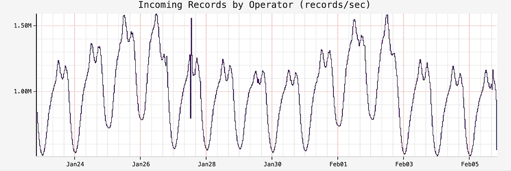
FlowExporter is a sidecar that runs alongside all Netflix workloads. It uses eBPF and TCP tracepoints to monitor TCP socket state changes. When a TCP socket closes, FlowExporter generates a flow log record that includes the IP addresses, ports, timestamps, and additional socket statistics. On average, 5 million records are produced per second.
In cloud environments, IP addresses are reassigned to different workloads as workload instances are created and terminated, so IP addresses alone cannot provide insights on which workloads are communicating. To make the flow logs useful, each IP address must be attributed to its corresponding workload identity. FlowCollector, a backend service, collects flow logs from FlowExporter instances across the fleet, attributes the IP addresses, and sends these attributed flows to Netflix’s Data Mesh for subsequent stream and batch processing.
The eBPF flow logs provide a comprehensive view of service topology and network health across Netflix’s extensive microservices fleet, regardless of the programming language, RPC mechanism, or application-layer protocol used by individual workloads.
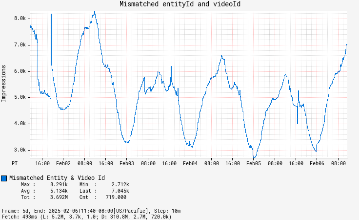
The Problem with Misattribution
Accurately attributing flow IP addresses to workload identities has been a significant challenge since our eBPF flow logs were introduced.
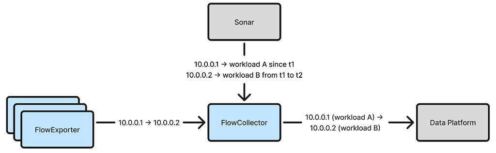
As noted in our previous blog post, our initial attribution approach relied on Sonar, an internal IP address tracking service that emits an event whenever an IP address in Netflix’s AWS VPCs is assigned or unassigned to a workload. FlowCollector consumes a stream of IP address change events from Sonar and uses this information to attribute flow IP addresses in real-time.
The fundamental drawback of this method is that it can lead to misattribution. Delays and failures are inevitable in distributed systems, which may delay IP address change events from reaching FlowCollector. For instance, an IP address may initially be assigned to workload X but later reassigned to workload Y. However, if the change event for this reassignment is delayed, FlowCollector will continue to assume that the IP address belongs to workload X, resulting in misattributed flows. Additionally, event timestamps may be inaccurate depending on how they are captured.
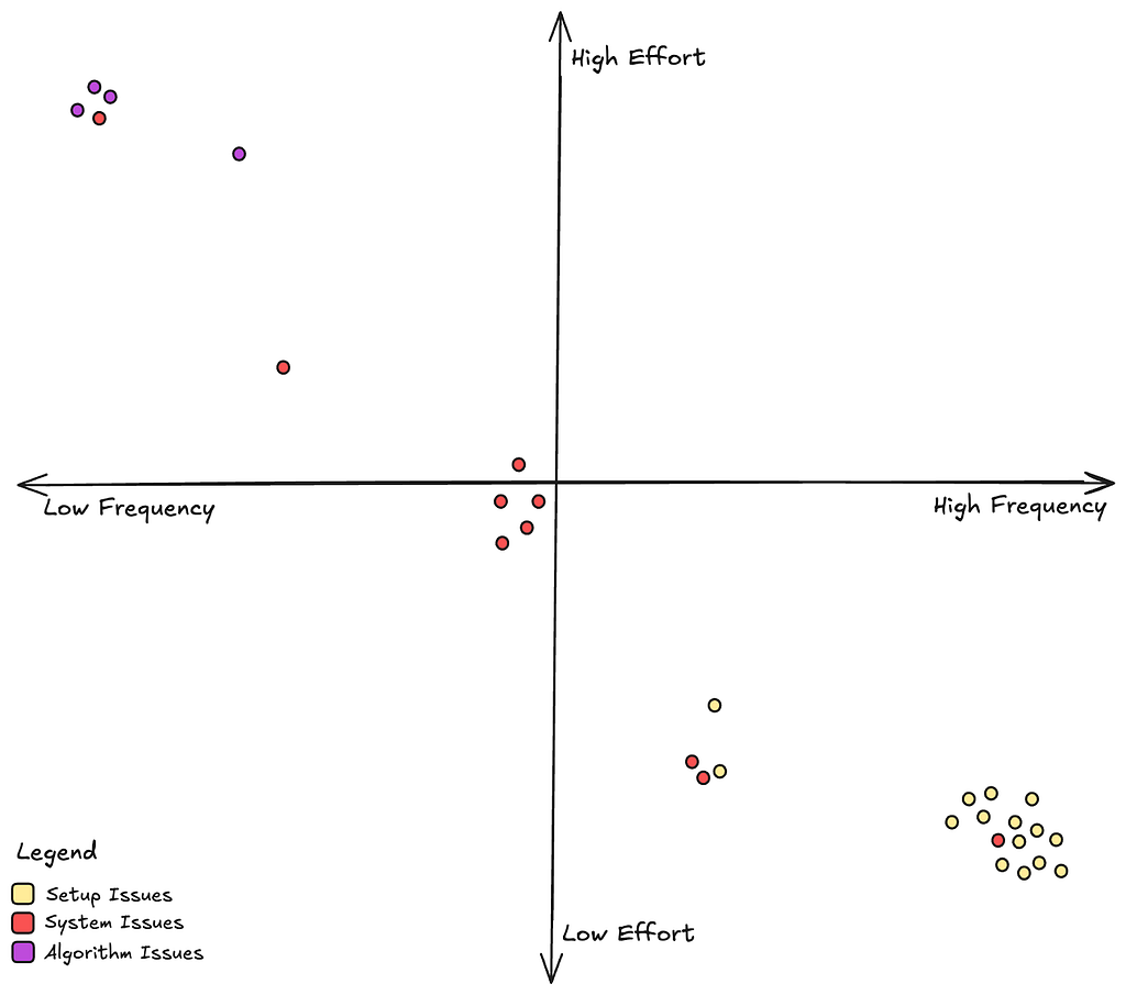
Misattribution rendered the flow data unreliable for decision-making. Users often depend on flow logs to validate workload dependencies, but misattribution creates confusion. Without expert knowledge of expected dependencies, users would struggle to identify or confirm misattribution. Moreover, misattribution occurred frequently for critical services with a large footprint due to frequent IP address changes. Overall, misattribution makes fleet-wide dependency analysis impractical.
As a workaround, we made FlowCollector hold received flows for 15 minutes before attribution, allowing time for delayed IP address change events. While this approach reduced misattribution, it did not eliminate it. Moreover, the waiting period made the data less fresh, reducing its utility for real-time analysis.
Fully eliminating misattribution is crucial because it only takes a single misattributed flow to produce an incorrect workload dependency. Solving this problem required a complete rethinking of our approach. Over the past year, Netflix developed a new attribution method that has finally eliminated misattribution, as detailed in the rest of this post.
Attributing Local IP Addresses
Each socket has two IP addresses: a local IP address and a remote IP address. Previously, we used the same method to attribute both. However, attributing the local IP address should be a simpler task since the local IP address belongs to the instance where FlowExporter captures the socket. Therefore, FlowExporter should determine the local workload identity from its environment and attribute the local IP address before sending the flow to FlowCollector.
This is straightforward for workloads running directly on EC2 instances, as Netflix’s Metatron provisions workload identity certificates to each EC2 instance at boot time. FlowExporter can simply read these certificates from the local disk to determine the local workload identity.
Attributing local IP addresses for container workloads running on Netflix’s container platform, Titus, is more challenging. FlowExporter runs at the container host level, where each host manages multiple container workloads with different identities. When FlowExporter’s eBPF programs receive a socket event from TCP tracepoints in the kernel, the socket may have been created by one of the container workloads or by the host itself. Therefore, FlowExporter must determine which workload to attribute the socket’s local IP address to. To solve this problem, we leveraged IPMan, Netflix’s container IP address assignment service. IPManAgent, a daemon running on every container host, is responsible for assigning and unassigning IP addresses. As container workloads are launched, IPManAgent writes an IP-address-to-workload-ID mapping to an eBPF map, which FlowExporter’s eBPF programs can then use to look up the workload ID associated with a socket local IP address.
Another challenge was to accommodate Netflix’s IPv6 to IPv4 translation mechanism on Titus. To facilitate IPv6 migration, Netflix developed a mechanism that enables IPv6-only containers to communicate with IPv4 destinations without incurring NAT64 overhead. This mechanism intercepts connect syscalls and replaces the underlying socket with one that uses a shared IPv4 address assigned to the container host. This confuses FlowExporter because the kernel reports the same local IPv4 address for sockets created by different container workloads. To disambiguate, local port information is additionally required. We modified Titus to write a mapping of (local IPv4 address, local port) to the workload ID into an eBPF map whenever a connect syscall is intercepted. FlowExporter’s eBPF programs then use this map to correctly attribute sockets created by the translation mechanism.
With these problems solved, we can now accurately attribute the local IP address of every flow.
Attributing Remote IP Addresses
Once the local IP address attribution problem is solved, accurately attributing remote IP addresses becomes feasible. Now, each flow reported by FlowExporter includes the local IP address, the local workload identity, and connection start/end timestamps. As FlowCollector receives these flows, it can learn the time ranges during which each workload owns a given IP address. For instance, if FlowCollector sees a flow with local IP address 10.0.0.1 associated with workload X that starts at t1 and ends at t2, it can deduce that 10.0.0.1 belonged to workload X from t1 to t2. Since Netflix uses Amazon Time Sync across its fleet, the timestamps (captured by FlowExporter) are reliable.
The FlowCollector service cluster consists of many nodes. Every node must be capable of attributing arbitrary remote IP addresses and, therefore, requires knowledge of all workload IP addresses and their recent ownership records. To represent this knowledge, each node maintains an in-memory hashmap that maps an IP address to a list of time ranges, as illustrated by the following Go structs:
type IPAddressTracker struct {
    ipToTimeRanges map[netip.Addr]timeRanges
}

type timeRanges []timeRange

type timeRange struct {
    workloadID   string
    start        time.Time
    end          time.Time
}
To populate the hashmap, FlowCollector extracts the local IP address, local workload identity, start time, and end time from each received flow and creates/extends the corresponding time ranges in the map. The time ranges for each IP address are sorted in ascending order, and they are non-overlapping since an IP address cannot belong to two different workloads simultaneously.
Since each flow is only sent to one FlowCollector node, each node must share the time ranges it learned from received flows with other nodes. We implemented a broadcasting mechanism using Kafka, where each node publishes learned time ranges to all other nodes. Although more efficient broadcasting implementations exist, the Kafka-based approach is simple and has worked well for us.
Now, FlowCollector can attribute remote IP addresses by looking them up in the populated map, which returns a list of time ranges. It then uses the flow’s start timestamp to determine the corresponding time range and associated workload identity. If the start time does not fall within any time range, FlowCollector will retry after a delay, eventually giving up if the retry fails. Such failures may occur when flows are lost or broadcast messages are delayed. For our use cases, it is acceptable to leave a small percentage of flows unattributed, but any misattribution is unacceptable.
This new method achieves accurate attribution thanks to the continuous heartbeats, each associated with a reliable time range of IP address ownership. It handles transient issues gracefully — a few delayed or lost heartbeats do not lead to misattribution. In contrast, the previous method relied solely on discrete IP address assignment and unassignment events. Lacking heartbeats, it had to presume an IP address remained assigned until notified otherwise (which can be hours or days later), making it vulnerable to misattribution when the notifications were delayed.
One detail is that when FlowCollector receives a flow, it cannot attribute its remote IP address right away because it requires the latest observed time ranges for the remote IP address. Since FlowExporter reports flows in batches every minute, FlowCollector must wait until it receives the flow batch from the remote workload FlowExporter for the last minute, which may not have arrived yet. To address this, FlowCollector temporarily stores received flows on disk for one minute before attributing their remote IP addresses. This introduces a 1-minute delay, but it is much shorter than the 15-minute delay with the previous approach.
In addition to producing accurate attribution, the new method is also cost-effective thanks to its simplicity and in-memory lookups. Because the in-memory state can be quickly rebuilt when a FlowCollector node starts up, no persistent storage is required. With 30 c7i.2xlarge instances, we can process 5 million flows per second across the entire Netflix fleet.
Attributing Cross-Regional IP Addresses
For simplicity, we have so far glossed over one topic: regionalization. Netflix’s cloud microservices operate across multiple AWS regions. To optimize flow reporting and minimize cross-regional traffic, a FlowCollector cluster runs in each major region, and FlowExporter agents send flows to their corresponding regional FlowCollector. When FlowCollector receives a flow, its local IP address is guaranteed to be within the region.
To minimize cross-region traffic, the broadcasting mechanism is limited to FlowCollector nodes within the same region. Consequently, the IP address time ranges map contains only IP addresses from that region. However, cross-regional flows have a remote IP address in a different region. To attribute these flows, the receiving FlowCollector node forwards them to nodes in the corresponding region. FlowCollector determines the region for a remote IP address by looking up a trie built from all Netflix VPC CIDRs. This approach is more efficient than broadcasting IP address time range updates across all regions, as only 1% of Netflix flows are cross-regional.
Attributing Non-Workload IP Addresses
So far, FlowCollector can accurately attribute IP addresses belonging to Netflix’s cloud workloads. However, not all flow IP addresses fall into this category. For instance, a significant portion of flows goes through AWS ELBs. For these flows, their remote IP addresses are associated with the ELBs, where we cannot run FlowExporter. Consequently, FlowCollector cannot determine their identities by simply observing the received flows. To attribute these remote IP addresses, we continue to use IP address change events from Sonar, which crawls AWS resources to detect changes in IP address assignments. Although this data stream may contain inaccurate timestamps and be delayed, misattribution is not a main concern since ELB IP address reassignment occurs very infrequently.
Verifying Correctness
Verifying that the new method has eliminated misattribution is challenging due to the lack of a definitive source of truth for workload dependencies to validate flow logs against; the flow logs themselves are intended to serve as this source of truth, after all. To build confidence, we analyzed the flow logs of a large service with well-understood dependencies. A large footprint is necessary, as misattribution is more prevalent in services with numerous instances, and there must be a reliable method to determine the dependencies for this service without relying on flow logs.
Netflix’s cloud gateway, Zuul, served this purpose perfectly due to its extensive footprint (handling all cloud ingress traffic), its large number of downstream dependencies, and our ability to derive its dependencies from its routing configurations as the source of truth for comparison with flow logs. We found no misattribution for flows through Zuul over a two-week window. This provided strong confidence that the new attribution method has eliminated misattribution. In the previous approach, approximately 40% of Zuul’s dependencies reported by the flow logs were misattributed.
Conclusion
With misattribution solved, eBPF flow logs now deliver dependable, fleet-wide insights into Netflix’s service topology and network health. This advancement unlocks numerous exciting opportunities in areas such as service dependency auditing, security analysis, and incident triage, while helping Netflix engineers develop a better understanding of our ever-evolving distributed systems.
The journey from script to screen is full of challenges in the ever-evolving world of film and television. The industry has always innovated, and over the last decade, it started moving towards cloud-based workflows. However, unlocking cloud innovation and all its benefits on a global scale has proven to be difficult. The opportunity is clear: streamline complex media management logistics, eliminate tedious, non-creative task-based work and enable productions to focus on what matters most–creative storytelling. With these challenges in mind, Netflix has developed a suite of tools by filmmakers for filmmakers: the Media Production Suite (MPS).
What are we solving for?
Significant time and resources are devoted to managing media logistics throughout the production lifecycle. An average Netflix title produces around ~200 Terabytes of Original Camera Files (OCF), with outliers up to 700 Terabytes, not including any work-in-progress files, VFX assets, 3D assets, etc. The data produced on set is traditionally copied to physical tape stock like LTO. This workflow has been considered the industry norm for a long time and may be cost-effective, but comes with trade-offs. Aside from needing to physically ship and track all movement of the tape stock, storing media on a physical tape makes it harder to search, play and share media assets; slowing down accessibility to production media when needed, especially when titles need to collaborate with talent and vendors all over the world.
Even when workflows are fully digital, the distribution of media between multiple departments and vendors can still be challenging. A lack of automation and standardization often results in a labour-intensive process across post-production and VFX with a lot of dependencies that introduce potential human errors and security risks. Many productions utilize a large variety of vendors, making this collaboration a large technical puzzle. As file sizes grow and workflows become more complex, these issues are magnified, leading to inefficiencies that slow down post-production and reduce the available time spent on creative work.
Moving media into the cloud introduces new challenges for production and post ramping up to meet the operational and technological hurdles this poses. For some post-production facilities, it’s not uncommon to see a wall of portable hard drives at their facility, with media being hand-carried between vendors because alternatives are not available. The need for a centralized, cloud-based solution that transcends these barriers is more pressing than ever. This results in a willingness to embrace new and innovative ideas, even if exploratory, and introduce drastic workflow changes to productions in pursuit of creative evolution.
At Netflix, we believe that great stories can come from anywhere, but we have seen that technical limitations in traditional workflows reduce access to media and restrict filmmakers’ access to talent. Besides the need for robust cloud storage for their media, artists need access to powerful workstations and real-time playback. Depending on the market, or production budget, cutting-edge technology might not be available or affordable.
What if we started charting a course to break free from many of these technical limitations and found ways to enhance creativity? Industry trade shows like the International Broadcast Convention (IBC) and the National Association of Broadcasters Show (NAB) highlight a strong global trend: instead of bringing media to the artist/applications (traditional workflow) we see the shift towards bringing people and applications to the media (cloud workflows and remote workstations). The concept of cloud-based workflows is not new, as many technology leaders in our industry have been experimenting in this space for more than a decade. However, executing this vision at a Netflix scale with hundreds of titles a year has not been done before…
The challenge of building a global technology to solve this
Building solutions at a global scale poses significant challenges. The art of making movies and series lacks equal access to technology, best practices, and global standardization. Different countries worldwide are at different phases of innovation based on local needs and nuances. While some regions boast over a century of cinematic history and have a strong industry, others are just beginning to carve their niche. This vast gap presents a unique challenge: developing global technology that caters to both established and emerging markets, each with distinct languages and workflows.
The large diversity of needs by talent and vendors globally creates a standardization challenge and can be seen when productions use a global talent pool. Many mature post-production and VFX facilities have built scripts and automation that flow between various artists and personnel within their facility; allowing a more streamlined workflow, even though the customization is time-consuming. E.g., Transcoding, or transcriptions that automatically run when files are dropped in a hot folder, with the expectation that certain sidecar metadata files will accompany them with a specific organizational structure. Embracing and integrating new workflows introduces the fear of disrupting a well-established process, increasing additional pressure on the profit margins of vendors. Small workflow changes that may seem arbitrary may actually have a large impact on vendors. Therefore, innovation should provide meaningful benefits to a title in order to get adopted at scale. Reliability, a proven track record, strong support, and an incredibly low tolerance for bugs, or issues are top of mind in well-established markets.
In developing this suite, we recognized the necessity of addressing the vast array of titles that flow through Netflix without the luxury of expanding into a massive operational entity. Consequently, automation became imperative. The intricacies of color and framing management, along with deliverables, must be seamlessly controlled and effortlessly managed by the user, without the need for manual intervention. Therefore, we cannot lean into humans configuring JSON files behind the scenes to map camera formats into deliverables. By embracing open standards, we not only streamline these processes but also facilitate smoother collaboration across diverse markets and countries, ensuring that our global productions can operate with unparalleled efficiency and cohesion. To ensure this, we’ve decided to lean heavily into standards like ACES, AMF, ASC MHL, ASC FDL, and OTIO. ACES and AMF for color pipeline management. ASC MHL for any file management/verifications. ASC FDL will serve as our framing interoperability and OTIO for any timeline interchange. Leaning into standards like this means that many things can be automated at scale and more importantly, high-complexity workflows can be offered to markets or shows that don’t normally have access to them. As an example, if a show is shot on various camera formats all framed and recorded at different resolutions, with different lenses and different safeties on each frame. The task of normalizing all of these for a VFX vendor into one common container with a normalized center extracted frame is often only offered to very high-end titles, considering it takes a human behind the curtain to create all of these mappings. But by leaning into a standard like the FDL, it means this can now easily be automated, and the control for these mappings, put directly in the hands of users.
Our Answer — Content Hub’s Media Production Suite (MPS)
Building a global scalable solution that could be utilized in a diversity of markets has been an exciting challenge. We set out to provide customizable and feature-rich tooling for advanced users while remaining intuitive and streamlined enough for less experienced filmmakers. With collaboration from Netflix teams, vendors, and talent across the globe, we’ve taken a bold step forward in enabling a suite of tools inside Netflix Content Hub that democratizes technology: the Media Production Suite. While leveraging our scale economies and access to resources, we can now unlock global talent pools for our productions, drastically reduce non-creative task-based work, streamline workflows, and level the playing field between our markets, ultimately maximizing the time available for what matters most; creative work!
So what is it?
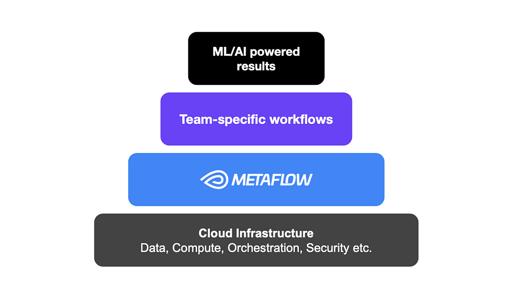
1. Netflix Hybrid Infrastructure: Netflix has invested in a hybrid infrastructure, a mix of cloud-based and physically distributed capabilities operating in multiple locations across the world and close to our productions to optimize user performance. This infrastructure is available for Netflix shows and is foundational under Content Hub’s Media Production Suite tooling. Local storage and compute services are connected through the Netflix Open Connect network (Netflix Content Delivery Network) to the infrastructure of Amazon Web Services (AWS). The system facilitates large volumes of camera and sound media and is built for speed. In order to ensure that productions have sufficient upload speeds to get their media into the cloud, Netflix has started to roll out Content Hub Ingest Centers globally to provide high-speed internet connectivity where required. With all media centralized, MPS eliminates the need for physical media transport and reduces the risk of human error. This approach not only streamlines operations but also enhances security and accessibility.
2. Automation and Tooling: In addition to the Netflix Hybrid infrastructure layer, MPS consists of a suite of tools that tap into the media in the Netflix ecosystem.
Footage Ingest — An application that allows users to upload media/files into Content Hub.
Media Library — A central library that allows users to search, preview, share and download media.
Dailies — A workflow, backed by an operational team, offering automated Quality Control of your footage, sound sync, application of color, rendering, and delivering dailies directly to editorial.
Remote Workstations — Offering access to remote editorial workstations and storage for post-production needs.
VFX Pulls — An automated method for converting and delivering visual effects plates, associated color, and framing files to VFX vendors.
Conform Pulls — An automated method for consolidating, trimming, and delivering all OCF to picture-finishing vendors.
Media Downloader — An automated download tool that initiates a download once media has been made available in the Netflix cloud.
While each of the individual tools within MPS is at different states of maturity, over 350 titles have made use of at least one of the tools noted above. Input has been taken from all over the world while developing, with users ranging from UCAN (United States/Canada), EMEA (Europe, Middle East, and Africa), SEA (South East Asia), LATAM (Latin America), and APAC (Asia Pacific).
Senna: Early Adoption and Insightful Feedback Driving MPS Evolution
Media from the Brazilian-produced series ‘Senna’ being reviewed in MPS
The Brazilian-produced series Senna, which follows the life of legendary Formula 1 driver Ayrton Senna, utilized MPS to reshape their content creation workflow, overcome geographical barriers, and unlock innovation to support world-class storytelling for a global audience. Senna is a groundbreaking series, not just for its storytelling but for its production journey across Argentina, Uruguay, Brazil, and the United Kingdom. With editorial teams spread across Porto Alegre and Spain, and VFX studios collaborating across locations in Brazil, Canada, the United States, and India, all orchestrated by our subsidiary Scanline VFX. The series exemplifies the global nature of modern filmmaking and was the perfect fit for Netflix’s new Content Hub Media Production Suite (MPS).
At the heart of Senna’s workflow orchestration is MPS. While each of the tools within MPS is based on an opt-in model, in order to use many of the downstream services, the first step is ensuring that the original camera files (OCF) and original sound files (OSF) are uploaded. “We knew we were going to shoot in different places,” said Post Supervisor Gabriel Queiroz,“to have all this material cloud-based, it’s definitely one of the most important things for us. It would be hard to bring all this media physically from Argentina or wherever to Brazil. It will take us a lot of time.” With Senna shooting across locations, allowing production the capability of uploading their OCF and OSF resulted in no longer requiring shuttling hard drives on airplanes, creating LTO tapes, & managing physical shipments for their negative. And yes, you read that correctly; when utilizing MPS, we don’t require LTO tapes to be written unless there are title-specific needs.
With Senna beginning production back in June of 2023, our investment in MPS was still very early stages, and the tooling was considered beta. However, with the help, feedback, and partnership from this production, it was quickly realized that the investment was worth doubling down on. Since the early version used on Senna, Netflix has been spinning up ingest centers around the world, where drives can be dropped off, and within a matter of hours, all original camera files are uploaded into the Netflix ecosystem. While creating the ability to upload is not a novel concept, behind the scenes, it’s far from simple. Once a drive has been plugged in and our Netflix Footage Ingest application is opened, a validation is run, ensuring all expected media from set is on the drive. After media has been uploaded and checksums are run validating media integrity, all media is inspected, metadata is extracted, and assets are created for viewing/sharing/downloading with playable proxies. All media is then automatically backed up to a second tier of cloud-based storage for the final archive.
Traditionally, if you wanted to check in with your post vendor on how things are going for each of these media management steps noted above, or whether or not you can clear on set camera cards if you haven’t gotten a completion notification, you would have to pick up the phone and call your vendor. For Senna, anyone who wanted visibility on progress, simply logged in to Content Hub and could see any activity in the Footage Ingest dashboard, as well as look up any information needed on past uploads.
Remote monitoring media being uploaded and archived using the MPS Footage Ingest workflow
While many services in MPS are available once media has been uploaded, Senna’s use of MPS focused on VFX. With Senna shooting a high volume of footage and the show having a high volume of VFX shots, according to Post Supervisor Gabriel Queiroz “Using MPS was basically a no-brainer, [having] used the tool before, I knew what it could bring to the project. And to be honest, with the amount of footage that we have, it was just so much material and with the amount of vendors we have, knowing that we would have to deliver all this footage to all these kinds of vendors, including outside of Brazil and to different parts of the world.”
With a traditional workflow, utilizing available resources in Latin America, VFX Pulls would have been done manually. This process is prone to human error and more importantly, for a show like Senna, too slow and would have resulted in different I/O methods for every vendor.
Illustrating a traditional VFX Editor having to manage various I/O methods
By utilizing MPS, the Assistant Editor was able to log into Content Hub, upload an EDL, and have their VFX Pulls automatically transcoded, color files consolidated and all media placed into a Google Drive style folder built directly in Content Hub (called Workspaces). The VFX Editor was able to make any additional tweaks they wanted to the directory before farming out each of the shots to whichever vendor they were meant for. When it came time for the VFX vendors to then send shots back to editorial or DI, this was also done through MPS. Having one standard method for I/O for all VFX file sharing meant that Editorial and DI did not have to manage a different file transfer/workflow for every single vendor that was onboarded.
Illustrating a more streamlined workflow for VFX vendors when using MPS
After picture was locked and it was time for Senna to do their Online, the DI facility Quanta was able to utilize the Conform Pull service within MPS. The Conform Pull service allowed their team to upload an EDL, which ran a QC on all of the media from within their edit to ensure a smooth conform and then consolidated, trimmed, and packaged up all of the media they needed for the online. Since this early beta and thanks to learnings from many shows like Senna, advancements have been made in the system’s ability to match back to source media for both Conform and VFX Pulls. Rather than requiring an exact match between EDL and source OCF, there are several variations of fuzzy matching that can take place, as well as a current investigation in using one of our perceptual matching algorithms, allowing for a perceptual conform using computer vision, instead of solely relying on metadata.
Conclusion
The Media Production Suite (MPS) represents a transformative leap in how we approach media production at Netflix. By embracing open standards, we have crafted a scalable solution that not only makes economic sense but also democratizes access to advanced production tools across the globe. This approach allows us to eliminate tedious tasks, enabling our teams to focus on what truly matters: creative storytelling. By fostering global collaboration and leveraging the power of cloud-based workflows, we’re not just enhancing efficiency but also elevating the quality of our productions. As we continue to innovate and refine our processes, we remain committed to breaking down barriers and unlocking the full potential of creative talent worldwide. The future of filmmaking is here, and with MPS, we are leading the charge toward a more connected and creatively empowered industry.
Netflix’s personalized recommender system is a complex system, boasting a variety of specialized machine learned models each catering to distinct needs including “Continue Watching” and “Today’s Top Picks for You.” (Refer to our recent overview for more details). However, as we expanded our set of personalization algorithms to meet increasing business needs, maintenance of the recommender system became quite costly. Furthermore, it was difficult to transfer innovations from one model to another, given that most are independently trained despite using common data sources. This scenario underscored the need for a new recommender system architecture where member preference learning is centralized, enhancing accessibility and utility across different models.
Particularly, these models predominantly extract features from members’ recent interaction histories on the platform. Yet, many are confined to a brief temporal window due to constraints in serving latency or training costs. This limitation has inspired us to develop a foundation model for recommendation. This model aims to assimilate information both from members’ comprehensive interaction histories and our content at a very large scale. It facilitates the distribution of these learnings to other models, either through shared model weights for fine tuning or directly through embeddings.
The impetus for constructing a foundational recommendation model is based on the paradigm shift in natural language processing (NLP) to large language models (LLMs). In NLP, the trend is moving away from numerous small, specialized models towards a single, large language model that can perform a variety of tasks either directly or with minimal fine-tuning. Key insights from this shift include:
A Data-Centric Approach: Shifting focus from model-centric strategies, which heavily rely on feature engineering, to a data-centric one. This approach prioritizes the accumulation of large-scale, high-quality data and, where feasible, aims for end-to-end learning.
Leveraging Semi-Supervised Learning: The next-token prediction objective in LLMs has proven remarkably effective. It enables large-scale semi-supervised learning using unlabeled data while also equipping the model with a surprisingly deep understanding of world knowledge.
These insights have shaped the design of our foundation model, enabling a transition from maintaining numerous small, specialized models to building a scalable, efficient system. By scaling up semi-supervised training data and model parameters, we aim to develop a model that not only meets current needs but also adapts dynamically to evolving demands, ensuring sustainable innovation and resource efficiency.
Data
At Netflix, user engagement spans a wide spectrum, from casual browsing to committed movie watching. With over 300 million users at the end of 2024, this translates into hundreds of billions of interactions — an immense dataset comparable in scale to the token volume of large language models (LLMs). However, as in LLMs, the quality of data often outweighs its sheer volume. To harness this data effectively, we employ a process of interaction tokenization, ensuring meaningful events are identified and redundancies are minimized.
Tokenizing User Interactions: Not all raw user actions contribute equally to understanding preferences. Tokenization helps define what constitutes a meaningful “token” in a sequence. Drawing an analogy to Byte Pair Encoding (BPE) in NLP, we can think of tokenization as merging adjacent actions to form new, higher-level tokens. However, unlike language tokenization, creating these new tokens requires careful consideration of what information to retain. For instance, the total watch duration might need to be summed or engagement types aggregated to preserve critical details.
Figure 1.Tokenization of user interaction history by merging actions on the same title, preserving important information.
This tradeoff between granular data and sequence compression is akin to the balance in LLMs between vocabulary size and context window. In our case, the goal is to balance the length of interaction history against the level of detail retained in individual tokens. Overly lossy tokenization risks losing valuable signals, while too granular a sequence can exceed practical limits on processing time and memory.
Even with such strategies, interaction histories from active users can span thousands of events, exceeding the capacity of transformer models with standard self attention layers. In recommendation systems, context windows during inference are often limited to hundreds of events — not due to model capability but because these services typically require millisecond-level latency. This constraint is more stringent than what is typical in LLM applications, where longer inference times (seconds) are more tolerable.
To address this during training, we implement two key solutions:
Sparse Attention Mechanisms: By leveraging sparse attention techniques such as low-rank compression, the model can extend its context window to several hundred events while maintaining computational efficiency. This enables it to process more extensive interaction histories and derive richer insights into long-term preferences.
Sliding Window Sampling: During training, we sample overlapping windows of interactions from the full sequence. This ensures the model is exposed to different segments of the user’s history over multiple epochs, allowing it to learn from the entire sequence without requiring an impractically large context window.
At inference time, when multi-step decoding is needed, we can deploy KV caching to efficiently reuse past computations and maintain low latency.
These approaches collectively allow us to balance the need for detailed, long-term interaction modeling with the practical constraints of model training and inference, enhancing both the precision and scalability of our recommendation system.
Information in Each ‘Token’: While the first part of our tokenization process focuses on structuring sequences of interactions, the next critical step is defining the rich information contained within each token. Unlike LLMs, which typically rely on a single embedding space to represent input tokens, our interaction events are packed with heterogeneous details. These include attributes of the action itself (such as locale, time, duration, and device type) as well as information about the content (such as item ID and metadata like genre and release country). Most of these features, especially categorical ones, are directly embedded within the model, embracing an end-to-end learning approach. However, certain features require special attention. For example, timestamps need additional processing to capture both absolute and relative notions of time, with absolute time being particularly important for understanding time-sensitive behaviors.
To enhance prediction accuracy in sequential recommendation systems, we organize token features into two categories:
Request-Time Features: These are features available at the moment of prediction, such as log-in time, device, or location.
Post-Action Features: These are details available after an interaction has occurred, such as the specific show interacted with or the duration of the interaction.
To predict the next interaction, we combine request-time features from the current step with post-action features from the previous step. This blending of contextual and historical information ensures each token in the sequence carries a comprehensive representation, capturing both the immediate context and user behavior patterns over time.
Considerations for Model Objective and Architecture
As previously mentioned, our default approach employs the autoregressive next-token prediction objective, similar to GPT. This strategy effectively leverages the vast scale of unlabeled user interaction data. The adoption of this objective in recommendation systems has shown multiple successes [1–3]. However, given the distinct differences between language tasks and recommendation tasks, we have made several critical modifications to the objective.
Firstly, during the pretraining phase of typical LLMs, such as GPT, every target token is generally treated with equal weight. In contrast, in our model, not all user interactions are of equal importance. For instance, a 5-minute trailer play should not carry the same weight as a 2-hour full movie watch. A greater challenge arises when trying to align long-term user satisfaction with specific interactions and recommendations. To address this, we can adopt a multi-token prediction objective during training, where the model predicts the next n tokens at each step instead of a single token[4]. This approach encourages the model to capture longer-term dependencies and avoid myopic predictions focused solely on immediate next events.
Secondly, we can use multiple fields in our input data as auxiliary prediction objectives in addition to predicting the next item ID, which remains the primary target. For example, we can derive genres from the items in the original sequence and use this genre sequence as an auxiliary target. This approach serves several purposes: it acts as a regularizer to reduce overfitting on noisy item ID predictions, provides additional insights into user intentions or long-term genre preferences, and, when structured hierarchically, can improve the accuracy of predicting the target item ID. By first predicting auxiliary targets, such as genre or original language, the model effectively narrows down the candidate list, simplifying subsequent item ID prediction.
Unique Challenges for Recommendation FM
In addition to the infrastructure challenges posed by training bigger models with substantial amounts of user interaction data that are common when trying to build foundation models, there are several unique hurdles specific to recommendations to make them viable. One of unique challenges is entity cold-starting.
At Netflix, our mission is to entertain the world. New titles are added to the catalog frequently. Therefore the recommendation foundation models require a cold start capability, which means the models need to estimate members’ preferences for newly launched titles before anyone has engaged with them. To enable this, our foundation model training framework is built with the following two capabilities: Incremental training and being able to do inference with unseen entities.
Incremental training : Foundation models are trained on extensive datasets, including every member’s history of plays and actions, making frequent retraining impractical. However, our catalog and member preferences continually evolve. Unlike large language models, which can be incrementally trained with stable token vocabularies, our recommendation models require new embeddings for new titles, necessitating expanded embedding layers and output components. To address this, we warm-start new models by reusing parameters from previous models and initializing new parameters for new titles. For example, new title embeddings can be initialized by adding slight random noise to existing average embeddings or by using a weighted combination of similar titles’ embeddings based on metadata. This approach allows new titles to start with relevant embeddings, facilitating faster fine-tuning. In practice, the initialization method becomes less critical when more member interaction data is used for fine-tuning.
Dealing with unseen entities : Even with incremental training, it’s not always guaranteed to learn efficiently on new entities (ex: newly launched titles). It’s also possible that there will be some new entities that are not included/seen in the training data even if we fine-tune foundation models on a frequent basis. Therefore, it’s also important to let foundation models use metadata information of entities and inputs, not just member interaction data. Thus, our foundation model combines both learnable item id embeddings and learnable embeddings from metadata. The following diagram demonstrates this idea.
Figure 2. Titles are associated with various metadata, such as genres, storylines, and tones. Each type of metadata could be represented by averaging its respective embeddings, which are then concatenated to form the overall metadata-based embedding for the title.
To create the final title embedding, we combine this metadata-based embedding with a fully-learnable ID-based embedding using a mixing layer. Instead of simply summing these embeddings, we use an attention mechanism based on the “age” of the entity. This approach allows new titles with limited interaction data to rely more on metadata, while established titles can depend more on ID-based embeddings. Since titles with similar metadata can have different user engagement, their embeddings should reflect these differences. Introducing some randomness during training encourages the model to learn from metadata rather than relying solely on ID embeddings. This method ensures that newly-launched or pre-launch titles have reasonable embeddings even with no user interaction data.
Downstream Applications and Challenges
Our recommendation foundation model is designed to understand long-term member preferences and can be utilized in various ways by downstream applications:
Direct Use as a Predictive Model The model is primarily trained to predict the next entity a user will interact with. It includes multiple predictor heads for different tasks, such as forecasting member preferences for various genres. These can be directly applied to meet diverse business needs..
Utilizing embeddings The model generates valuable embeddings for members and entities like videos, games, and genres. These embeddings are calculated in batch jobs and stored for use in both offline and online applications. They can serve as features in other models or be used for candidate generation, such as retrieving appealing titles for a user. High-quality title embeddings also support title-to-title recommendations. However, one important consideration is that the embedding space has arbitrary, uninterpretable dimensions and is incompatible across different model training runs. This poses challenges for downstream consumers, who must adapt to each retraining and redeployment, risking bugs due to invalidated assumptions about the embedding structure. To address this, we apply an orthogonal low-rank transformation to stabilize the user/item embedding space, ensuring consistent meaning of embedding dimensions, even as the base foundation model is retrained and redeployed.
Fine-Tuning with Specific Data The model’s adaptability allows for fine-tuning with application-specific data. Users can integrate the full model or subgraphs into their own models, fine-tuning them with less data and computational power. This approach achieves performance comparable to previous models, despite the initial foundation model requiring significant resources.
Scaling Foundation Models for Netflix Recommendations
In scaling up our foundation model for Netflix recommendations, we draw inspiration from the success of large language models (LLMs). Just as LLMs have demonstrated the power of scaling in improving performance, we find that scaling is crucial for enhancing generative recommendation tasks. Successful scaling demands robust evaluation, efficient training algorithms, and substantial computing resources. Evaluation must effectively differentiate model performance and identify areas for improvement. Scaling involves data, model, and context scaling, incorporating user engagement, external reviews, multimedia assets, and high-quality embeddings. Our experiments confirm that the scaling law also applies to our foundation model, with consistent improvements observed as we increase data and model size.
Figure 3. The relationship between model parameter size and relative performance improvement. The plot demonstrates the scaling law in recommendation modeling, showing a trend of increased performance with larger model sizes. The x-axis is logarithmically scaled to highlight growth across different magnitudes.
Conclusion
In conclusion, our Foundation Model for Personalized Recommendation represents a significant step towards creating a unified, data-centric system that leverages large-scale data to increase the quality of recommendations for our members. This approach borrows insights from Large Language Models (LLMs), particularly the principles of semi-supervised learning and end-to-end training, aiming to harness the vast scale of unlabeled user interaction data. Addressing unique challenges, like cold start and presentation bias, the model also acknowledges the distinct differences between language tasks and recommendation. The Foundation Model allows various downstream applications, from direct use as a predictive model to generate user and entity embeddings for other applications, and can be fine-tuned for specific canvases. We see promising results from downstream integrations. This move from multiple specialized models to a more comprehensive system marks an exciting development in the field of personalized recommendation systems.
C. K. Kang and J. McAuley, “Self-Attentive Sequential Recommendation,” 2018 IEEE International Conference on Data Mining (ICDM), Singapore, 2018, pp. 197–206, doi: 10.1109/ICDM.2018.00035.
F. Sun et al., “BERT4Rec: Sequential Recommendation with Bidirectional Encoder Representations from Transformer,” Proceedings of the 28th ACM International Conference on Information and Knowledge Management (CIKM ‘19), Beijing, China, 2019, pp. 1441–1450, doi: 10.1145/3357384.3357895.
J. Zhai et al., “Actions Speak Louder than Words: Trillion-Parameter Sequential Transducers for Generative Recommendations,” arXiv preprint arXiv:2402.17152, 2024.
F. Gloeckle, B. Youbi Idrissi, B. Rozière, D. Lopez-Paz, and G. Synnaeve, “Better & Faster Large Language Models via Multi-token Prediction,” arXiv preprint arXiv:2404.19737, Apr. 2024.
We are excited to announce that we are now streaming HDR10+ content on our service for AV1-enabled devices, enhancing the viewing experience for certified HDR10+ devices, which previously only received HDR10 content. The dynamic metadata included in our HDR10+ content improves the quality and accuracy of the picture when viewed on these devices.
Delighting Members with Even Better Picture Quality
Nearly a decade ago, we made a bold move to be a pioneering adopter of High Dynamic Range (HDR) technology. HDR enables images to have more details, vivid colors, and improved realism. We began producing our shows and movies in HDR, encoding them in HDR, and streaming them in HDR for our members. We were confident that it would greatly enhance our members’ viewing experience, and unlock new creative visions — and we were right! In the last five years, HDR streaming has increased by more than 300%, while the number of HDR-configured devices watching Netflix has more than doubled. Since launching HDR with season one of Marco Polo, Netflix now has over 11,000 hours of HDR titles for members to immerse themselves in.
We continue to enhance member joy while maintaining creative vision by adding support for HDR10+. This will further augment Netflix’s growing HDR ecosystem, preserve creative intent on even more devices, and provide a more immersive viewing experience.
We enabled HDR10+ on Netflix using the AV1 video codec that was standardized by the Alliance for Open Media (AOM) in 2018. AV1 is one of the most efficient codecs available today. We previously enabled AV1 encoding for SDR content, and saw tremendous value for our members, including higher and more consistent visual quality, lower play delay and increased streaming at the highest resolution. AV1-SDR is already the second most streamed codec at Netflix, behind H.264/AVC, which has been around for over 20 years! With the addition of HDR10+ streams to AV1, we expect the day is not far when AV1 will be the most streamed codec at Netflix.
To enhance our offering, we have been adding HDR10+ streams to both new releases and existing popular HDR titles. AV1-HDR10+ now accounts for 50% of all eligible viewing hours. We will continue expanding our HDR10+ offerings with the goal of providing an HDR10+ experience for all HDR titles by the end of this year¹.
Industry Adopted Formats
Today, the industry recognizes three prevalent HDR formats: Dolby Vision, HDR10, and HDR10+. For all three HDR Formats, metadata is embedded in the content, serving as instructions to guide the playback device — whether it’s a TV, mobile device, or computer — on how to display the image.
HDR10 is the most widely adopted HDR format, supported by all HDR devices. HDR10 uses static metadata that is defined once for the entire content detailing aspects such as the maximum content light level (MaxCLL), maximum frame average light level (MaxFALL), as well as characteristics of the mastering display used for color grading. This metadata only allows for a one-size-fits-all tone mapping of the content for display devices. It cannot account for dynamic contrast across scenes, which most content contains.
HDR10+ and Dolby Vision improve on this with dynamic metadata that provides content image statistics on a per-frame basis, enabling optimized tone mapping adjustments for each scene. This achieves greater perceptual fidelity to the original, preserving creative intent.
HDR10 vs. HDR10+
The figure below shows screen grabs of two AV1-encoded frames of the same content displayed using HDR10 (top) and HDR10+ (bottom).
Photographs of devices displaying the same frame with HDR10 metadata (top) and HDR10+ metadata (bottom). Notice the preservation of the flashlight detail in the HDR10+ capture, and the over-exposure of the region under the flashlight in the HDR10 one².
As seen in the flashlight on the table, the highlight details are clipped in the HDR10 content, but are recovered in HDR10+. Further, the region under the flashlight is overexposed in the HDR10 content, while HDR10+ renders that region with greater fidelity to the source. The reason HDR10+, with its dynamic metadata, shines in this example is that the scenes preceding and following the scene with this frame have markedly different luminance statistics. The static HDR10 metadata is unable to account for the change in the content. While this is a simple example, the dynamic metadata in HDR10+ demonstrates such value across any set of scenes. This consistency allows our members to stay immersed in the content, and better preserves creative intent.
Receiving HDR10+
At the time of launch, these requirements must be satisfied to receive HDR10+:
1.Member must have a Netflix Premium plan subscription
2. Title must be available in HDR10+ format
3. Member device must support AV1 & HDR10+. Here are some examples of compatible devices:
SmartTVs, mobile phones, and tablets that meet Netflix certification for HDR10+
Source device (such as set-top boxes, streaming devices, MVPDs, etc.) that meets Netflix certification for HDR10+, connected to an HDR10+ compliant display via HDMI
More HDR content is watched every day on Netflix. Expanding the Netflix HDR ecosystem to include HDR10+ increases the accessibility of HDR content with dynamic metadata to more members, improves the viewing experience, and preserves the creative intent of our content creators. The commitment to innovation and quality underscores our dedication to delivering an immersive and authentic viewing experience for all our members.
Acknowledgements
Launching HDR10+ was a collaborative effort involving multiple teams at Netflix, and we are grateful to everyone who contributed to making this idea a reality. We would like to extend our thanks to the following teams for their crucial roles in this launch:
The Encoding Technologies team that is responsible for producing optimized encodings to enable high-quality experiences for our members. Special acknowledgments: Adithya Prakash, Vinicius Carvalho
The Content Operations & Innovation teams responsible for producing and delivering HDR content to Netflix, maintaining the intent of creative vision from production to streaming. Special acknowledgements: Michael Keegan
Footnotes
While we have enabled HDR10+ for distribution i.e., for what our members consume on their devices, we continue to accept only Dolby Vision masters on the ingest side, i.e., for all content delivery to Netflix as per our delivery specification. In addition to HDR10+, we continue to serve HDR10 and DolbyVision. Our encoding pipeline is designed with flexibility and extensibility where all these HDR formats could be derived from a single DolbyVision deliverable efficiently at scale.
We recognize that it is hard to convey visual improvements in HDR video using still photographs converted to SDR. We encourage the reader to stream Netflix content in HDR10+ and check for yourself!
This blog post is a continuation of Part 2, where we cleared the ambiguity around title launch observability at Netflix. In this installment, we will explore the strategies, tools, and methodologies that were employed to achieve comprehensive title observability at scale.
Defining the observability endpoint
To create a comprehensive solution, we decided to introduce observability endpoints first. Each microservice involved in our Personalization stack that integrated with our observability solution had to introduce a new “Title Health” endpoint. Our goal was for each new endpoint to adhere to a few principles:
Accurate reflection of production behavior
Standardization across all endpoints
Answering the Insight Triad: “Healthy” or not, why not and how to fix it.
Accurately Reflecting Production Behavior
A key part of our solution is insights into production behavior, which necessitates our requests to the endpoint result in traffic to the real service functions that mimics the same pathways the traffic would take if it came from the usual callers.
In order to allow for this mimicking, many systems implement an “event” handling, where they convert our request into a call to the real service with properties enabled to log when titles are filtered out of their response and why. Building services that adhere to software best practices, such as Object-Oriented Programming (OOP), the SOLID principles, and modularization, is crucial to have success at this stage. Without these practices, service endpoints may become tightly coupled to business logic, making it challenging and costly to add a new endpoint that seamlessly integrates with the observability solution while following the same production logic.
A service with modular business logic facilitates the seamless addition of an observability endpoint.
Standardization
To standardize communication between our observability service and the personalization stack’s observability endpoints, we’ve developed a stable proto request/response format. This centralized format, defined and maintained by our team, ensures all endpoints adhere to a consistent protocol. As a result, requests are uniformly handled, and responses are processed cohesively. This standardization enhances adoption within the personalization stack, simplifies the system, and improves understanding and debuggability for engineers.
The request schema for the observability endpoint.
The Insight Triad API
To efficiently understand the health of a title and triage issues quickly, all implementations of the observability endpoint must answer: is the title eligible for this phase of promotion, if not — why is it not eligible, and what can be done to fix any problems.
The end-users of this observability system are Launch Managers, whose job it is to ensure smooth title launches. As such, they must be able to quickly see whether there is a problem, what the problem is, and how to solve it. Teams implementing the endpoint must provide as much information as possible so that a non-engineer (Launch Manager) can understand the root cause of the issue and fix any title setup issues as they arise. They must also provide enough information for partner engineers to identify the problem with the underlying service in cases of system-level issues.
These requirements are captured in the following protobuf object that defines the endpoint response.
The response schema for the observability endpoint.
High level architecture
We’ve distilled our comprehensive solution into the following key steps, capturing the essence of our approach:
Establish observability endpoints across all services within our Personalization and Discovery Stack.
Implement proactive monitoring for each of these endpoints.
Track real-time title impressions from the Netflix UI.
Store the data in an optimized, highly distributed datastore.
Offer easy-to-integrate APIs for our dashboard, enabling stakeholders to track specific titles effectively.
“Time Travel” to validate ahead of time.
Observability stack high level architecture diagram
In the following sections, we will explore each of these concepts and components as illustrated in the diagram above.
Key Features
Proactive monitoring through scheduled collectors jobs
Our Title Health microservice runs a scheduled collector job every 30 minutes for most of our personalization stack.
For each Netflix row we support (such as Trending Now, Coming Soon, etc.), there is a dedicated collector. These collectors retrieve the relevant list of titles from our catalog that qualify for a specific row by interfacing with our catalog services. These services are informed about the expected subset of titles for each row, for which we are assessing title health.
Once a collector retrieves its list of candidate titles, it orchestrates batched calls to assigned row services using the above standardized schema to retrieve all the relevant health information of the titles. Additionally, some collectors will instead poll our kafka queue for impressions data.
Real-time Title Impressions and Kafka Queue
In addition to evaluating title health via our personalization stack services, we also keep an eye on how our recommendation algorithms treat titles by reviewing impressions data. It’s essential that our algorithms treat all titles equitably, for each one has limitless potential.
This data is processed from a real-time impressions stream into a Kafka queue, which our title health system regularly polls. Specialized collectors access the Kafka queue every two minutes to retrieve impressions data. This data is then aggregated in minute(s) intervals, calculating the number of impressions titles receive in near-real-time, and presented as an additional health status indicator for stakeholders.
Data storage and distribution through Hollow Feeds
Netflix Hollow is an Open Source java library and toolset for disseminating in-memory datasets from a single producer to many consumers for high performance read-only access. Given the shape of our data, hollow feeds are an excellent strategy to distribute the data across our service boxes.
Once collectors gather health data from partner services in the personalization stack or from our impressions stream, this data is stored in a dedicated Hollow feed for each collector. Hollow offers numerous features that help us monitor the overall health of a Netflix row, including ensuring there are no large-scale issues across a feed publish. It also allows us to track the history of each title by maintaining a per-title data history, calculate differences between previous and current data versions, and roll back to earlier versions if a problematic data change is detected.
Observability Dashboard using Health Check Engine
We maintain several dashboards that utilize our title health service to present the status of titles to stakeholders. These user interfaces access an endpoint in our service, enabling them to request the current status of a title across all supported rows. This endpoint efficiently reads from all available Hollow Feeds to obtain the current status, thanks to Hollow’s in-memory capabilities. The results are returned in a standardized format, ensuring easy support for future UIs.
Additionally, we have other endpoints that can summarize the health of a title across subsets of sections to highlight specific member experiences.
Message depicting a dashboard request.
Time Traveling: Catching before launch
Titles launching at Netflix go through several phases of pre-promotion before ultimately launching on our platform. For each of these phases, the first several hours of promotion are critical for the reach and effective personalization of a title, especially once the title has launched. Thus, to prevent issues as titles go through the launch lifecycle, our observability system needs to be capable of simulating traffic ahead of time so that relevant teams can catch and fix issues before they impact members. We call this capability “Time Travel”.
Many of the metadata and assets involved in title setup have specific timelines for when they become available to members. To determine if a title will be viewable at the start of an experience, we must simulate a request to a partner service as if it were from a future time when those specific metadata or assets are available. This is achieved by including a future timestamp in our request to the observability endpoint, corresponding to when the title is expected to appear for a given experience. The endpoint then communicates with any further downstream services using the context of that future timestamp.
An example request with a future timestamp.
Conclusion
Throughout this series, we’ve explored the journey of enhancing title launch observability at Netflix. In Part 1, we identified the challenges of managing vast content launches and the need for scalable solutions to ensure each title’s success. Part 2 highlighted the strategic approach to navigating ambiguity, introducing “Title Health” as a framework to align teams and prioritize core issues. In this final part, we detailed the sophisticated system strategies and architecture, including observability endpoints, proactive monitoring, and “Time Travel” capabilities; all designed to ensure a thrilling viewing experience.
By investing in these innovative solutions, we enhance the discoverability and success of each title, fostering trust with content creators and partners. This journey not only bolsters our operational capabilities but also lays the groundwork for future innovations, ensuring that every story reaches its intended audience and that every member enjoys their favorite titles on Netflix.
Thank you for joining us on this exploration, and stay tuned for more insights and innovations as we continue to entertain the world.
Imagine scrolling through Netflix, where each movie poster or promotional banner competes for your attention. Every image you hover over isn’t just a visual placeholder; it’s a critical data point that fuels our sophisticated personalization engine. At Netflix, we call these images ‘impressions,’ and they play a pivotal role in transforming your interaction from simple browsing into an immersive binge-watching experience, all tailored to your unique tastes.
Capturing these moments and turning them into a personalized journey is no simple feat. It requires a state-of-the-art system that can track and process these impressions while maintaining a detailed history of each profile’s exposure. This nuanced integration of data and technology empowers us to offer bespoke content recommendations.
In this multi-part blog series, we take you behind the scenes of our system that processes billions of impressions daily. We will explore the challenges we encounter and unveil how we are building a resilient solution that transforms these client-side impressions into a personalized content discovery experience for every Netflix viewer.
Impressions on homepage
Why do we need impression history?
Enhanced Personalization
To tailor recommendations more effectively, it’s crucial to track what content a user has already encountered. Having impression history helps us achieve this by allowing us to identify content that has been displayed on the homepage but not engaged with, helping us deliver fresh, engaging recommendations.
Frequency Capping
By maintaining a history of impressions, we can implement frequency capping to prevent over-exposure to the same content. This ensures users aren’t repeatedly shown identical options, keeping the viewing experience vibrant and reducing the risk of frustration or disengagement.
Highlighting New Releases
For new content, impression history helps us monitor initial user interactions and adjust our merchandising efforts accordingly. We can experiment with different content placements or promotional strategies to boost visibility and engagement.
Analytical Insights
Additionally, impression history offers insightful information for addressing a number of platform-related analytics queries. Analyzing impression history, for example, might help determine how well a specific row on the home page is functioning or assess the effectiveness of a merchandising strategy.
Architecture Overview
The first pivotal step in managing impressions begins with the creation of a Source-of-Truth (SOT) dataset. This foundational dataset is essential, as it supports various downstream workflows and enables a multitude of use cases.
Collecting Raw Impression Events
As Netflix members explore our platform, their interactions with the user interface spark a vast array of raw events. These events are promptly relayed from the client side to our servers, entering a centralized event processing queue. This queue ensures we are consistently capturing raw events from our global user base.
After raw events are collected into a centralized queue, a custom event extractor processes this data to identify and extract all impression events. These extracted events are then routed to an Apache Kafka topic for immediate processing needs and simultaneously stored in an Apache Iceberg table for long-term retention and historical analysis. This dual-path approach leverages Kafka’s capability for low-latency streaming and Iceberg’s efficient management of large-scale, immutable datasets, ensuring both real-time responsiveness and comprehensive historical data availability.
Collecting raw impression events
Filtering & Enriching Raw Impressions
Once the raw impression events are queued, a stateless Apache Flink job takes charge, meticulously processing this data. It filters out any invalid entries and enriches the valid ones with additional metadata, such as show or movie title details, and the specific page and row location where each impression was presented to users. This refined output is then structured using an Avro schema, establishing a definitive source of truth for Netflix’s impression data. The enriched data is seamlessly accessible for both real-time applications via Kafka and historical analysis through storage in an Apache Iceberg table. This dual availability ensures immediate processing capabilities alongside comprehensive long-term data retention.
Impression Source-of-Truth architecture
Ensuring High Quality Impressions
Maintaining the highest quality of impressions is a top priority. We accomplish this by gathering detailed column-level metrics that offer insights into the state and quality of each impression. These metrics include everything from validating identifiers to checking that essential columns are properly filled. The data collected feeds into a comprehensive quality dashboard and supports a tiered threshold-based alerting system. These alerts promptly notify us of any potential issues, enabling us to swiftly address regressions. Additionally, while enriching the data, we ensure that all columns are in agreement with each other, offering in-place corrections wherever possible to deliver accurate data.
Dashboard showing mismatch count between two columns- entityId and videoId
Configuration
We handle a staggering volume of 1 to 1.5 million impression events globally every second, with each event approximately 1.2KB in size. To efficiently process this massive influx in real-time, we employ Apache Flink for its low-latency stream processing capabilities, which seamlessly integrates both batch and stream processing to facilitate efficient backfilling of historical data and ensure consistency across real-time and historical analyses. Our Flink configuration includes 8 task managers per region, each equipped with 8 CPU cores and 32GB of memory, operating at a parallelism of 48, allowing us to handle the necessary scale and speed for seamless performance delivery. The Flink job’s sink is equipped with a data mesh connector, as detailed in our Data Mesh platform which has two outputs: Kafka and Iceberg. This setup allows for efficient streaming of real-time data through Kafka and the preservation of historical data in Iceberg, providing a comprehensive and flexible data processing and storage solution.
Raw impressions records per second
We utilize the ‘island model’ for deploying our Flink jobs, where all dependencies for a given application reside within a single region. This approach ensures high availability by isolating regions, so if one becomes degraded, others remain unaffected, allowing traffic to be shifted between regions to maintain service continuity. Thus, all data in one region is processed by the Flink job deployed within that region.
Future Work
Addressing the Challenge of Unschematized Events
Allowing raw events to land on our centralized processing queue unschematized offers significant flexibility, but it also introduces challenges. Without a defined schema, it can be difficult to determine whether missing data was intentional or due to a logging error. We are investigating solutions to introduce schema management that maintains flexibility while providing clarity.
Automating Performance Tuning with Autoscalers
Tuning the performance of our Apache Flink jobs is currently a manual process. The next step is to integrate with autoscalers, which can dynamically adjust resources based on workload demands. This integration will not only optimize performance but also ensure more efficient resource utilization.
Improving Data Quality Alerts
Right now, there’s a lot of business rules dictating when a data quality alert needs to be fired. This leads to a lot of false positives that require manual judgement. A lot of times it is difficult to track changes leading to regression due to inadequate data lineage information. We are investing in building a comprehensive data quality platform that more intelligently identifies anomalies in our impression stream, keeps track of data lineage and data governance, and also, generates alerts notifying producers of any regressions. This approach will enhance efficiency, reduce manual oversight, and ensure a higher standard of data integrity.
Conclusion
Creating a reliable source of truth for impressions is a complex but essential task that enhances personalization and discovery experience. Stay tuned for the next part of this series, where we’ll delve into how we use this SOT dataset to create a microservice that provides impression histories. We invite you to share your thoughts in the comments and continue with us on this journey of discovering impressions.
Acknowledgments
We are genuinely grateful to our amazing colleagues whose contributions were essential to the success of Impressions: Julian Jaffe, Bryan Keller, Yun Wang, Brandon Bremen, Kyle Alford, Ron Brown and Shriya Arora.
Building on the foundation laid in Part 1, where we explored the “what” behind the challenges of title launch observability at Netflix, this post shifts focus to the “how.” How do we ensure every title launches seamlessly and remains discoverable by the right audience?
In the dynamic world of technology, it’s tempting to leap into problem-solving mode. But the key to lasting success lies in taking a step back — understanding the broader context before diving into solutions. This thoughtful approach doesn’t just address immediate hurdles; it builds the resilience and scalability needed for the future. Let’s explore how this mindset drives results.
Understanding the Bigger Picture
Let’s take a comprehensive look at all the elements involved and how they interconnect. We should aim to address questions such as: What is vital to the business? Which aspects of the problem are essential to resolve? And how did we arrive at this point?
This process involves:
Identifying Stakeholders: Determine who is impacted by the issue and whose input is crucial for a successful resolution. In this case, the main stakeholders are:
– Title Launch Operators Role: Responsible for setting up the title and its metadata into our systems. Challenge: Don’t understand the cascading effects of their setup on these perceived black box personalization systems
– Personalization System Engineers Role: Develop and operate the personalization systems. Challenge: End up spending unplanned cycles on title launch and personalization investigations.
– Product Managers Role: Ensure we put forward the best experience for our members. Challenge: Members may not connect with the most relevant title.
– Creative Representatives Role: Mediator between the content creators and Netflix. Challenge: Build trust in the Netflix brand with content creators.
Mapping the Current Landscape: By charting the existing landscape, we can pinpoint areas ripe for improvement and steer clear of redundant efforts. Beyond the scattered solutions and makeshift scripts, it became evident that there was no established solution for title launch observability. This suggests that this area has been neglected for quite some time and likely requires significant investment. This situation presents both challenges and opportunities; while it may be more difficult to make initial progress, there are plenty of easy wins to capitalize on.
Clarifying the Core Problem: By clearly defining the problem, we can ensure that our solutions address the root cause rather than just the symptoms. While there were many issues and problems we could address, the core problem here was to make sure every title was treated fairly by our personalization stack. If we can ensure fair treatment with confidence and bring that visibility to all our stakeholders, we can address all their challenges.
Assessing Business Priorities: Understanding what is most important to the organization helps prioritize actions and resources effectively. In this context, we’re focused on developing systems that ensure successful title launches, build trust between content creators and our brand, and reduce engineering operational overhead. While this is a critical business need and we definitely should solve it, it’s essential to evaluate how it stacks up against other priorities across different areas of the organization.
Defining Title Health
Navigating such an ambiguous space required a shared understanding to foster clarity and collaboration. To address this, we introduced the term “Title Health,” a concept designed to help us communicate effectively and capture the nuances of maintaining each title’s visibility and performance. This shared language became a foundation for discussing the complexities of this domain.
“Title Health” encompasses various metrics and indicators that reflect how well a title is performing, in terms of discoverability and member engagement. The three main questions we try to answer are:
Is this title visible at all to anymember?
Is this title visible to an appropriate audience size?
Is this title reaching all the appropriate audiences?
Defining Title Health provided a framework to monitor and optimize each title’s lifecycle. It allowed us to align with partners on principles and requirements before building solutions, ensuring every title reaches its intended audience seamlessly. This common language not only introduced the problem space effectively but also accelerated collaboration and decision-making across teams.
Categories of issues
To build a robust plan for title launch observability, we first needed to categorize the types of issues we encounter. This structured approach allows us to address all aspects of title health comprehensively.
Currently, these issues are grouped into three primary categories:
1. Title Setup
A title’s setup includes essential attributes like metadata (e.g., launch dates, audio and subtitle languages, editorial tags) and assets (e.g., artwork, trailers, supplemental messages). These elements are critical for a title’s eligibility in a row, accurate personalization, and an engaging presentation. Since these attributes feed directly into algorithms, any delays or inaccuracies can ripple through the system.
The observability system must ensure that title setup is complete and validated in a timely manner, identify potential bottlenecks and ensure a smooth launch process.
2. Personalization Systems
Titles are eligible to be recommended across multiple canvases on product — HomePage, Coming Soon, Messaging, Search and more. Personalization systems handle the recommendation and serving of titles on these canvases, leveraging a vast ecosystem of microservices, caches, databases, code, and configurations to build these product canvases.
We aim to validate that titles are eligible in all appropriate product canvases across the end to end personalization stack during all of the title’s launch phases.
3. Algorithms
Complex algorithms drive each personalized product experience, recommending titles tailored to individual members. Observability here means validating the accuracy of algorithmic recommendations for all titles. Algorithmic performance can be affected by various factors, such as model shortcomings, incomplete or inaccurate input signals, feature anomalies, or interactions between titles. Identifying and addressing these issues ensures that recommendations remain precise and effective.
By categorizing issues into these areas, we can systematically address challenges and deliver a reliable, personalized experience for every title on our platform.
Issue Analysis
Let’s also learn more about how often we see each of these types of issues and how much effort it takes to fix them once they come up.
From the above chart, we see that setup issues are the most common but they are also easy to fix since it’s relatively straightforward to go back and rectify a title’s metadata. System issues, which mostly manifest as bugs in our personalization microservices are not uncommon, and they take moderate effort to address. Algorithm issues, while rare, are really difficult to address since these often involve interpreting and retraining complex machine learning models.
Evaluating Our Options
Now that we understand more deeply about the problems we want to address and how we should go about prioritizing our resources. Lets go back to the two options we discussed in Part 1, and make an informed decision.
Ultimately, we realized this space demands the full spectrum of features we’ve discussed. But the question remained: Where do we start? After careful consideration, we chose to focus on proactive issue detection first. Catching problems before launch offered the greatest potential for business impact, ensuring smoother launches, better member experiences, and stronger system reliability.
This decision wasn’t just about solving today’s challenges — it was about laying the foundation for a scalable, robust system that can grow with the complexities of our ever-evolving platform.
Up next
In the next iteration we will talk about how to design an observability endpoint that works for all personalization systems. What are the main things to keep in mind while creating a microservice API endpoint? How do we ensure standardization? What is the architecture of the systems involved?
Keep an eye out for our next binge-worthy episode!
This article is the last in a multi-part series sharing a breadth of Analytics Engineering work at Netflix, recently presented as part of our annual internal Analytics Engineering conference. Need to catch up? Check out Part 1, which detailed how we’re empowering Netflix to efficiently produce and effectively deliver high quality, actionable analytic insights across the company and Part 2, which stepped through a few exciting business applications for Analytics Engineering. This post will go into aspects of technical craft.
What is design, and why does it matter? Often people think design is about how things look, but design is actually about how things work. Everything is designed, because we’re all making choices about how things work, but not everything is designed well. Good design doesn’t waste time or mental energy; instead, it helps the user achieve their goals.
When applying this to a dashboard application, the easiest way to use design effectively is to leverage existing patterns. (For example, people have learned that blue underlined text on a website means it’s a clickable link.) So knowing the arsenal of available patterns and what they imply is useful when making the choice of when to use which pattern.
First, to design a dashboard well, you need to understand your user.
Talk to your users throughout the entire product lifecycle. Talk to them early and often, through whatever means you can.
Understand their needs, ask why, then ask why again. Separate symptoms from problems from solutions.
Prioritize and clarify — less is more! Distill what you can build that’s differentiated and provides the most value to your user.
Here is a framework for thinking about what your users are trying to achieve. Where do your users fall on these axes? Don’t solve for multiple positions across these axes in a given view; if that exists, then create different views or potentially different dashboards.
Second, understanding your users’ mental models will allow you to choose how to structure your app to match. A few questions to ask yourself when considering the information architecture of your app include:
Do you have different user groups trying to accomplish different things? Split them into different apps or different views.
What should go together on a single page? All the information needed for a single user type to accomplish their “job.” If there are multiple jobs to be done, split each out onto its own page.
What should go together within a single section on a page? All the information needed to answer a single question.
Does your dashboard feel too difficult to use? You probably have too much information! When in doubt, keep it simple. If needed, hide complexity under an “Advanced” section.
Here are some general guidelines for page layouts:
Choose infinite scrolling vs. clicking through multiple pages depending on which option suits your users’ expectations better
Lead with the most-used information first, above the fold
Create signposts that cue the user to where they are by labeling pages, sections, and links
Use cards or borders to visually group related items together
Leverage nesting to create well-understood “scopes of control.” Specifically, users expect a controller object to affect children either: Below it (if horizontal) or To the right of it (if vertical)
Third, some tips and tricks can help you more easily tackle the unique design challenges that come with making interactive charts.
Titles: Make sure filters are represented in the title or subtitle of the chart for easy scannability and screenshot-ability.
Tooltips: Core details should be on the page, while the context in the tooltip is for deeper information. Annotate multiple points when there are only a handful of lines.
Annotations: Provide annotations on charts to explain shifts in values so all users can access that context.
Color: Limit the number of colors you use. Be consistent in how you use colors. Otherwise, colors lose meaning.
Onboarding: Separate out onboarding to your dashboard from routine usage.
Finally, it is important to note that these are general guidelines, but there is always room for interpretation and/or the use of good judgment to adapt them to suit your own product and use cases. At the end of the day, the most important thing is that a user can leverage the data insights provided by your dashboard to perform their work, and good design is a means to that end.
Learnings from Deploying an Analytics API at Netflix
At Netflix Studio, we operate at the intersection of art and science. Data is a tool that enhances decision-making, complementing the deep expertise and industry knowledge of our creative professionals.
One example is in production budgeting — namely, determining how much we should spend to produce a given show or movie. Although there was already a process for creating and comparing budgets for new productions against similar past projects, it was highly manual. We developed a tool that automatically selects and compares similar Netflix productions, flagging any anomalies for Production Finance to review.
To ensure success, it was essential that results be delivered in real-time and integrated seamlessly into existing tools. This required close collaboration among product teams, DSE, and front-end and back-end developers. We developed a GraphQL endpoint using Metaflow, integrating it into the existing budgeting product. This solution enabled data to be used more effectively for real-time decision-making.
We recently launched our MVP and continue to iterate on the product. Reflecting on our journey, the path to launch was complex and filled with unexpected challenges. As an analytics engineer accustomed to crafting quick solutions, I underestimated the effort required to deploy a production-grade analytics API.
Fig 1. My vague idea of how my API would workFig 2: Our actual solution
With hindsight, below are my key learnings.
Measure Impact and Necessity of Real-Time Results
Before implementing real-time analytics, assess whether real-time results are truly necessary for your use case. This can significantly impact the complexity and cost of your solution. Batch processing data may provide a similar impact and take significantly less time. It’s easier to develop and maintain, and tends to be more familiar for analytics engineers, data scientists, and data engineers.
Additionally, if you are developing a proof of concept, the upfront investment may not be worth it. Scrappy solutions can often be the best choice for analytics work.
Explore All Available Solutions
At Netflix, there were multiple established methods for creating an API, but none perfectly suited our specific use case. Metaflow, a tool developed at Netflix for data science projects, already supported REST APIs. However, this approach did not align with the preferred workflow of our engineering partners. Although they could integrate with REST endpoints, this solution presented inherent limitations. Large response sizes rendered the API/front-end integration unreliable, necessitating the addition of filter parameters to reduce the response size.
Additionally, the product we were integrating into was using GraphQL, and deviating from this established engineering approach was not ideal. Lastly, given our goal to overlay results throughout the product, GraphQL features, such as federation, proved to be particularly advantageous.
After realizing there wasn’t an existing solution at Netflix for deploying python endpoints with GraphQL, we worked with the Metaflow team to build this feature. This allowed us to continue developing via Metaflow and allowed our engineering partners to stay on their paved path.
Align on Performance Expectations
A major challenge during development was managing API latency. Much of this could have been mitigated by aligning on performance expectations from the outset. Initially, we operated under our assumptions of what constituted an acceptable response time, which differed greatly from the actual needs of our users and our engineering partners.
Understanding user expectations is key to designing an effective solution. Our methodology resulted in a full budget analysis taking, on average, 7 seconds. Users were willing to wait for an analysis when they modified a budget, but not every time they accessed one. To address this, we implemented caching using Metaflow, reducing the API response time to approximately 1 second for cached results. Additionally, we set up a nightly batch job to pre-cache results.
While users were generally okay with waiting for analysis during changes, we had to be mindful of GraphQL’s 30-second limit. This highlighted the importance of continuously monitoring the impact of changes on response times, leading us to our next key learning: rigorous testing.
Real-Time Analysis Requires Rigorous Testing
Load Testing: We leveraged Locust to measure the response time of our endpoint and assess how the endpoint responded to reasonable and elevated loads. We were able to use FullStory, which was already being used in the product, to estimate expected calls per minute.
Fig 3. Locust allows us to simulate concurrent calls and measure response time
Unit Tests & Integration Tests: Code testing is always a good idea, but it can often be overlooked in analytics. It is especially important when you are delivering live analysis to circumvent end users from being the first to see an error or incorrect information. We implemented unit testing and full integration tests, ensuring that our analysis would return correct results.
The Importance of Aligning Workflows and Collaboration
This project marked the first time our team collaborated directly with our engineering partners to integrate a DSE API into their product. Throughout the process, we discovered significant gaps in our understanding of each other’s workflows. Assumptions about each other’s knowledge and processes led to misunderstandings and delays.
Deployment Paths: Our engineering partners followed a strict deployment path, whereas our approach on the DSE side was more flexible. We typically tested our work on feature branches using Metaflow projects and then pushed results to production. However, this lack of control led to issues, such as inadvertently deploying changes to production before the corresponding product updates were ready and difficulties in managing a test endpoint. Ultimately, we deferred to our engineering partners to establish a deployment path and collaborated with the Metaflow team and data engineers to implement it effectively.
Fig 4. Our current deployment path
Work Planning: While the engineering team operated on sprints, our DSE team planned by quarters. This misalignment in planning cycles is an ongoing challenge that we are actively working to resolve.
Looking ahead, our team is committed to continuing this partnership with our engineering colleagues. Both teams have invested significant time in building this relationship, and we are optimistic that it will yield substantial benefits in future projects.
External Speaker: Benn Stancil
In addition to the above presentations, we kicked off our Analytics Summit with a keynote talk from Benn Stancil, Founder of Mode Analytics. Benn stepped through a history of the modern data stack, and the group discussed ideas on the future of analytics.
Analytics Engineering is a key contributor to building our deep data culture at Netflix, and we are proud to have a large group of stunning colleagues that are not only applying but advancing our analytical capabilities at Netflix. The 2024 Analytics Summit continued to be a wonderful way to give visibility to one another on work across business verticals, celebrate our collective impact, and highlight what’s to come in analytics practice at Netflix.
This article is the second in a multi-part series sharing a breadth of Analytics Engineering work at Netflix, recently presented as part of our annual internal Analytics Engineering conference. Need to catch up? Check out Part 1. In this article, we highlight a few exciting analytic business applications, and in our final article we’ll go into aspects of the technical craft.
Netflix has been launching games for the past three years, during which it has initiated various marketing efforts, including User Acquisition (UA) campaigns, to promote these games across different countries. These UA campaigns typically feature static creatives, launch trailers, and game review videos on platforms like Google, Meta, and TikTok. The primary goals of these campaigns are to encourage more people to install and play the games, making incremental installs and engagement crucial metrics for evaluating their effectiveness.
Most UA campaigns are conducted at the country level, meaning that everyone in the targeted countries can see the ads. However, due to the absence of a control group in these countries, we adopt a synthetic control framework (blog post) to estimate the counterfactual scenario. This involves creating a weighted combination of countries not exposed to the UA campaign to serve as a counterfactual for the treated countries. To facilitate easier access to incrementality results, we have developed an interactive tool powered by this framework. This tool allows users to directly obtain the lift in game installs and engagement, view plots for both the treated country and the synthetic control unit, and assess the p-value from placebo tests.
To better guide the design and budgeting of future campaigns, we are developing an Incremental Return on Investment model. This model incorporates factors such as the incremental impact, the value of the incremental engagement and incremental signups, and the cost of running the campaign. In addition to using the causal inference framework mentioned earlier to estimate incrementality, we also leverage other frameworks, such as Incremental Account Lifetime Valuation (blog post), to assign value to the incremental engagement and signups resulting from the campaigns.
Measuring and Validating Incremental Signups for Netflix Games
Netflix is a subscription service meaning members buy subscriptions which include games but not the individual games themselves. This makes it difficult to measure the impact of different game launches on acquisition. We only observe signups, not why members signed up.
This means we need to estimate incremental signups. We adopt an approach developed at Netflix to estimate incremental acquisition (technical paper). This approach uses simple assumptions to estimate a counterfactual for the rate that new members start playing the game.
Because games differ from series/films, it’s crucial to validate this estimation method for games. Ideally, we would have causal estimates from an A/B test to use for validation, but since that is not available, we use another causal inference design as one of our ensemble of validation approaches. This causal inference design involves a systematic framework we designed to measure game events that relies on synthetic control (blog post).
As we mentioned above, we have been launching User Acquisition (UA) campaigns in select countries to boost game engagement and new memberships. We can use this cross-country variation to form a synthetic control and measure the incremental signups due to the UA campaign. The incremental signups from UA campaigns differ from those attributed to a game, but they should be similar. When our estimated incremental acquisition numbers over a campaign period are similar to the incremental acquisition numbers calculated using synthetic control, we feel more confident in our approach to measuring incremental signups for games.
Netflix Games Players’ Adventure: Modeled using State Machine
At Netflix Games, we aim to have a high number of members engaging with games each month, referred to as Monthly Active Accounts (MAA). To evaluate our progress toward this objective and to find areas to boost our MAA, we modeled the Netflix players’ journey as a state machine.
We track a daily state machine showing the probability of account transitions between states.
Fig: Netflix Players’ Journey as State machine
Modeling the players’ journey as a state machine allows us to simulate future states and assess progress toward engagement goals. The most basic operation involves multiplying the daily state-transition matrix with the current state values to determine the next day’s state values.
This basic operation allows us to explore various scenarios:
Constant Trends: If transition rates stay constant, we can predict future states by repeatedly multiplying the daily state-transition matrix to new state values, helping us assess progress towards annual goals under unchanged conditions.
Dynamic Scenarios: By modifying transition rates, we can simulate complex scenarios. For instance, mimicking past changes in transition rates from a game launch allows us to predict the impact of similar future launches by altering the transition rate for a specific period.
Steady State: We can calculate the steady state of the state-transition matrix (excluding new players) to estimate the MAA once all accounts have tried Netflix games and understand long-term retention and reactivation effects.
Beyond predicting future states, we use the state machine for sensitivity analysis to find which transition rates most impact MAA. By making small changes to each transition rate we calculate the resulting MAA and measure its impact. This guides us in prioritizing efforts on top-of-funnel improvements, member retention, or reactivation.
At Netflix we produce a variety of entertainment: movies, series, documentaries, stand-up specials, and more. Each format has a different production process and different patterns of cash spend, called our “Content Forecast”. Looking into the future, Netflix keeps a plan of how many titles we intend to produce, what kinds, and when. Because we don’t yet know what specific titles that content will eventually become, these generic placeholders are called “TBD Slots.” A sizable portion of our Content Forecast is represented by TBD Slots.
Almost all businesses have a cash forecasting process informing how much cash they need in a given time period to continue executing on their plans. As plans change, the cash forecast will change. Netflix has a cash forecast that projects our cash needs to produce the titles we plan to make. This presents the question: how can we optimally forecast cash needs for TBD Slots, given we don’t have details on what real titles they will become?
The large majority of our titles are funded throughout the production process — starting from when we begin developing the title to shooting the actual shows and movies to launch on our Netflix service.
Since cash spend is driven by what is happening on a production, we model it by breaking down into these three steps:
Determine estimated production phase durations using historical actuals
Determine estimated percent of cash spent in each production phase
Model the shape of cash spend within each phase
Putting these three pieces together allows us to generate a generic estimation of cash spend per day leading up to and beyond a title’s launch date (a proxy for “completion”). We could distribute this spend linearly across each phase, but this approach allows us to capture nuance around patterns of spend that ramp up slowly, or are concentrated at the start and taper off throughout.
Before starting any math, we need to ensure a high quality historical dataset. Data quality plays a huge role in this work. For example, if we see 80% of our cash spent before production even started, it might be safe to say that either the production dates (which are manually captured) are incorrect or that title had a unique spending pattern that we don’t want to anticipate our future titles will follow.
For the first two steps, finding the estimated phase durations and cash percent per phase, we’ve found that simple math works best, for interpretability and consistency. We use a weighted average across our “clean” historical actuals to produce these estimated assumptions.
For modeling the shape of spend throughout each phase, we perform constrained optimization to fit a 3rd degree polynomial function. The constraints include:
Must pass through the points (0,0) and (1,1). This ensures that 0% through the phase, 0% of that phase’s cash has been spent. Similarly, 100% through the phase, 100% of that phase’s cash has been spent.
The derivative must be non-negative. This ensures that the function is monotonically increasing, avoiding counterintuitively forecasting any negative spend.
The optimization’s objective function minimizes the sum of squared residuals and returns the coefficients of the polynomial that will guide the shape of cash spend through each phase.
Once we have these coefficients, we can evaluate this polynomial at each day of the expected phase duration, and then multiply the result by the expected cash per phase. With some additional data processing, this yields an expected percent of cash spend each day leading up to and beyond the launch date, which we can base our forecasts on.
Assistive Speech Recognition in Dubbing Workflows at Netflix
Great stories can come from anywhere and be loved everywhere. At Netflix, we strive to make our titles accessible to a global audience, transcending language barriers to connect with viewers worldwide. One of the key ways we achieve this is through creating dubs in many languages.
From the transcription of the original titles all the way to the delivery of the dub audio, we blend innovation with human expertise to preserve the original creative intent.
Leveraging technologies like Assistive Speech Recognition (ASR), we seek to make the transcription part of the process more efficient for our linguists. Transcription, in our context, involves creating a verbatim script of the spoken dialogue, along with precise timing information to perfectly align the text with the original video. With ASR, instead of starting the transcription from scratch, linguists get a pre-generated starting point which they can use and edit for complete accuracy.
This efficiency enables linguists to focus more on other creative tasks, such as adding cultural annotations and references, which are crucial for downstream dubbing.
With ASR, and other new and enhanced technologies we introduce, rigorous analytics and measurement are essential to their success. To effectively evaluate our ASR system, we’ve established a multi-layered measurement framework that provides comprehensive insights into its performance across many dimensions (for example, the accuracy of the text and timing predictions), offline and online.
ASR is expected to perform differently for various languages; therefore, at a high level, we track metrics by original language of the show, allowing us to assess overall ASR effectiveness and identify trends across different linguistic contexts. We further break down performance by various dimensions, e.g. content type, genre, etc… to help us pinpoint specific areas where the ASR system may encounter difficulties. Furthermore, our framework allows us to conduct in-depth analyses of individual titles’ transcription, focusing on critical quality dimensions around text and timing accuracy of ASR suggestions. By zooming in on where the system falls short, we gain valuable insights into specific challenges, enabling us to further refine our understanding of ASR performance.
These measurement layers collectively empower us to continuously monitor, identify improvement areas, and implement targeted enhancements, ensuring that our ASR technology gets more and more accurate, effective, and helpful to linguists across diverse content types and languages. By refining our dubbing workflows through these innovations, we aim to keep improving the quality of our dubs to help great stories travel across the globe and bring joy to our members.
Analytics Engineering is a key contributor to building our deep data culture at Netflix, and we are proud to have a large group of stunning colleagues that are not only applying but advancing our analytical capabilities at Netflix. The 2024 Analytics Summit continued to be a wonderful way to give visibility to one another on work across business verticals, celebrate our collective impact, and highlight what’s to come in analytics practice at Netflix.
A month ago at QConSF, we showcased how Netflix utilizes Metaflow to power a diverse set of ML and AI use cases, managing thousands of unique Metaflow flows. This followed a previous blog on the same topic. Many of these projects are under constant development by dedicated teams with their own business goals and development best practices, such as the system that supports our content decision makers, or the system that ranks which language subtitles are most valuable for a specific piece of content.
As a central ML and AI platform team, our role is to empower our partner teams with tools that maximize their productivity and effectiveness, while adapting to their specific needs (not the other way around). This has been a guiding design principle with Metaflow since its inception.
Metaflow infrastructure stack
Standing on the shoulders of our extensive cloud infrastructure, Metaflow facilitates easy access to data, compute, and production-grade workflow orchestration, as well as built-in best practices for common concerns such as collaboration, versioning, dependency management, and observability, which teams use to setup ML/AI experiments and systems that work for them. As a result, Metaflow users at Netflix have been able to run millions of experiments over the past few years without wasting time on low-level concerns.
A long standing FAQ: configurable flows
While Metaflow aims to be un-opinionated about some of the upper levels of the stack, some teams within Netflix have developed their own opinionated tooling. As part of Metaflow’s adaptation to their specific needs, we constantly try to understand what has been developed and, more importantly, what gaps these solutions are filling.
In some cases, we determine that the gap being addressed is very team specific, or too opinionated at too high a level in the stack, and we therefore decide to not develop it within Metaflow. In other cases, however, we realize that we can develop an underlying construct that aids in filling that gap. Note that even in that case, we do not always aim to completely fill the gap and instead focus on extracting a more general lower level concept that can be leveraged by that particular user but also by others. One such recurring pattern we noticed at Netflix is the need to deploy sets of closely related flows, often as part of a larger pipeline involving table creations, ETLs, and deployment jobs. Frequently, practitioners want to experiment with variants of these flows, testing new data, new parameterizations, or new algorithms, while keeping the overall structure of the flow or flows intact.
A natural solution is to make flows configurable using configuration files, so variants can be defined without changing the code. Thus far, there hasn’t been a built-in solution for configuring flows, so teams have built their bespoke solutions leveraging Metaflow’s JSON-typed Parameters, IncludeFile, and deploy-time Parameters or deploying their own home-grown solution (often with great pain). However, none of these solutions make it easy to configure all aspects of the flow’s behavior, decorators in particular.
Requests for a feature like Metaflow Config
Outside Netflix, we have seen similar frequently asked questions on the Metaflow community Slack as shown in the user quotes above:
how can I adjust the @resource requirements, such as CPU or memory, without having to hardcode the values in my flows?
how to adjust the triggering @schedule programmatically, so our production and staging deployments can run at different cadences?
New in Metaflow: Configs!
Today, to answer the FAQ, we introduce a new — small but mighty — feature in Metaflow: a Config object. Configs complement the existing Metaflow constructs of artifacts and Parameters, by allowing you to configure all aspects of the flow, decorators in particular, prior to any run starting. At the end of the day, artifacts, Parameters and Configs are all stored as artifacts by Metaflow but they differ in when they are persisted as shown in the diagram below:
Different data artifacts in Metaflow
Said another way:
An artifact is resolved and persisted to the datastore at the end of each task.
A parameter is resolved and persisted at the start of a run; it can therefore be modified up to that point. One common use case is to use triggers to pass values to a run right before executing. Parameters can only be used within your step code.
A config is resolved and persisted when the flow is deployed. When using a scheduler such as Argo Workflows, deployment happens when create’ing the flow. In the case of a local run, “deployment” happens just prior to the execution of the run — think of “deployment” as gathering all that is needed to run the flow. Unlike parameters, configs can be used more widely in your flow code, particularly, they can be used in step or flow level decorators as well as to set defaults for parameters. Configs can of course also be used within your flow.
As an example, you can specify a Config that reads a pleasantly human-readable configuration file, formatted as TOML. The Config specifies a triggering ‘@schedule’ and ‘@resource’ requirements, as well as application-specific parameters for this specific deployment:
[schedule]
cron = "0 * * * *"

[model]
optimizer = "adam"
learning_rate = 0.5

[resources]
cpu = 1
Using the newly released Metaflow 2.13, you can configure a flow with a Config like above, as demonstrated by this flow:
There is a lot going on in the code above, a few highlights:
you can refer to configs before they have been defined using ‘config_expr’.
you can define arbitrary parsers — using a string means the parser doesn’t even have to be present remotely!
From the developer’s point of view, Configs behave like dictionary-like artifacts. For convenience, they support the dot-syntax (when possible) for accessing keys, making it easy to access values in a nested configuration. You can also unpack the whole Config (or a subtree of it) with Python’s standard dictionary unpacking syntax, ‘**config’. The standard dictionary subscript notation is also available.
Since Configs turn into dictionary artifacts, they get versioned and persisted automatically as artifacts. You can access Configs of any past runs easily through the Client API. As a result, your data, models, code, Parameters, Configs, and execution environments are all stored as a consistent bundle — neatly organized in Metaflow namespaces — paving the way for easily reproducible, consistent, low-boilerplate, and now easily configurable experiments and robust production deployments.
More than a humble config file
While you can get far by accompanying your flow with a simple config file (stored in your favorite format, thanks to user-definable parsers), Configs unlock a number of advanced use cases. Consider these examples from the updated documentation:
You are not limited to using a single file: you can leverage a configuration manager like OmegaConf or Hydra to manage a hierarchy of cascading configuration files. You can also use a domain-specific tool for generating Configs, such as Netflix’s Metaboost which we cover below.
You can also generate configurations on the fly, e.g. fetch Configs from an external service, or inspect the execution environment, such as the current GIT branch, and include it as an extra piece of context in runs.
A major benefit of Config over previous more hacky solutions for configuring flows is that they work seamlessly with other features of Metaflow: you can run steps remotely and deploy flows to production, even when relying on custom parsers, without having to worry about packaging Configs or parsers manually or keeping Configs consistent across tasks. Configs also work with the Runner and Deployer.
The Hollywood principle: don’t call us, we’ll call you
When used in conjunction with a configuration manager like Hydra, Configs enable a pattern that is highly relevant for ML and AI use cases: orchestrating experiments over multiple configurations or sweeping over parameter spaces. While Metaflow has always supported sweeping over parameter grids easily using foreaches, it hasn’t been easily possible to alter the flow itself, e.g. to change @resources or @pypi/@conda dependencies for every experiment.
In a typical case, you trigger a Metaflow flow that consumes a configuration file, changing how a run behaves. With Hydra, you can invert the control: it is Hydra that decides what gets run based on a configuration file. Thanks to Metaflow’s new Runner and Deployer APIs, you can create a Hydra app that operates Metaflow programmatically — for instance, to deploy and execute hundreds of variants of a flow in a large-scale experiment.
Take a look at two interesting examples of this pattern in the documentation. As a teaser, this video shows Hydra orchestrating deployment of tens of Metaflow flows, each of which benchmarks PyTorch using a varying number of CPU cores and tensor sizes, updating a visualization of the results in real-time as the experiment progresses:
Metaboosting Metaflow — based on a true story
To give a motivating example of what configurations look like at Netflix in practice, let’s consider Metaboost, an internal Netflix CLI tool that helps ML practitioners manage, develop and execute their cross-platform projects, somewhat similar to the open-source Hydra discussed above but with specific integrations to the Netflix ecosystem. Metaboost is an example of an opinionated framework developed by a team already using Metaflow. In fact, a part of the inspiration for introducing Configs in Metaflow came from this very use case.
Metaboost serves as a single interface to three different internal platforms at Netflix that manage ETL/Workflows (Maestro), Machine Learning Pipelines (Metaflow) and Data Warehouse Tables (Kragle). In this context, having a single configuration system to manage a ML project holistically gives users increased project coherence and decreased project risk.
Configuration in Metaboost
Ease of configuration and templatizing are core values of Metaboost. Templatizing in Metaboost is achieved through the concept of bindings, wherein we can bind a Metaflow pipeline to an arbitrary label, and then create a corresponding bespoke configuration for that label. The binding-connected configuration is then merged into a global set of configurations containing such information as GIT repository, branch, etc. Binding a Metaflow, will also signal to Metaboost that it should instantiate the Metaflow flow once per binding into our orchestration cluster.
Imagine a ML practitioner on the Netflix Content ML team, sourcing features from hundreds of columns in our data warehouse, and creating a multitude of models against a growing suite of metrics. When a brand new content metric comes along, with Metaboost, the first version of the metric’s predictive model can easily be created by simply swapping the target column against which the model is trained.
Subsequent versions of the model will result from experimenting with hyper parameters, tweaking feature engineering, or conducting feature diets. Metaboost’s bindings, and their integration with Metaflow Configs, can be leveraged to scale the number of experiments as fast as a scientist can create experiment based configurations.
Scaling experiments with Metaboost bindings — backed by Metaflow Config
Consider a Metaboost ML project named `demo` that creates and loads data to custom tables (ETL managed by Maestro), and then trains a simple model on this data (ML Pipeline managed by Metaflow). The project structure of this repository might look like the following:
Metaboost will merge each experiment configuration (*.EXP*.yaml) into the global configuration (settings.configuration.yaml) individually at Metaboost command initialization. Let’s take a look at how Metaboost combines these configurations with a Metaboost command:
(venv-demo) ~/projects/metaboost-demo [branch=demoX]
$ metaboost metaflow settings show --yaml-path=configuration

binding=EXP_01:
model:                     -> defined in setting.configuration.yaml (global)
  fit_intercept: true
conda:                     -> defined in setting.configuration.yaml (global)
  numpy: 1.22.4
  "scikit-learn": 1.4.0
target_column: metricA     -> defined in setting.configuration.EXP_01.yaml
features:                  -> defined in setting.configuration.EXP_01.yaml
- runtime
- content_type
- top_billed_talent

binding=EXP_02:
model:                     -> defined in setting.configuration.yaml (global)
  fit_intercept: true
conda:                     -> defined in setting.configuration.yaml (global)
  numpy: 1.22.4
  "scikit-learn": 1.4.0
target_column: metricA     -> defined in setting.configuration.EXP_02.yaml
features:                  -> defined in setting.configuration.EXP_02.yaml
- runtime
- director
- box_office
Metaboost understands it should deploy/run two independent instances of training.py — one for the EXP_01 binding and one for the EXP_02 binding. You can also see that Metaboost is aware that the tables and ETL workflows are not bound, and should only be deployed once. These details of which artifacts to bind and which to leave unbound are encoded in the project’s top-level metaboost.yaml file.
(venv-demo) ~/projects/metaboost-demo [branch=demoX] $ metaboost project list
Below is a simple Metaflow pipeline that fetches data, executes feature engineering, and trains a LinearRegression model. The work to integrate Metaboost Settings into a user’s Metaflow pipeline (implemented using Metaflow Configs) is as easy as adding a single mix-in to the FlowSpec definition:
from metaflow import FlowSpec, Parameter, conda_base, step from custom.data import feature_engineer, get_data from metaflow.metaboost import MetaboostSettings
@step def start(self): # get show_settings() for free with the mixin # and get convenient debugging info self.show_settings(exclude_patterns=["artifact*", "system*"])
self.next(self.get_features)
@step def get_features(self): # feature engineers on our extracted data self.fe_df = feature_engineer( # loads data from our ETL pipeline data=get_data(prediction_date=self.prediction_date), features=self.settings.configuration.features + [self.settings.configuration.target_column] )
self.next(self.train)
@step def train(self): from sklearn.linear_model import LinearRegression
The Metaflow Config is added to the FlowSpec by mixing in the MetaboostSettings class. Referencing a configuration value is as easy as using the dot syntax to drill into whichever parameter you’d like.
Finally let’s take a look at the output from our sample Metaflow above. We execute experiment EXP_01 with
metaboost metaflow run --binding=EXP_01
which upon execution will merge the configurations into a single settings file (shown previously) and serialize it as a yaml file to the .metaboost/settings/compiled/ directory.
You can see the actual command and args that were sub-processed in the Metaboost Execution section below. Please note the –config argument pointing to the serialized yaml file, and then subsequently accessible via self.settings. Also note the convenient printing of configuration values to stdout during the start step using a mixed in function named show_settings().
(venv-demo) ~/projects/metaboost-demo [branch=demoX] $ metaboost metaflow run --binding=EXP_01
Metaflow 2.12.39+nflxfastdata(2.13.5);nflx(2.13.5);metaboost(0.0.27) executing DemoTraining for user:dcasler Validating your flow... The graph looks good! Bootstrapping Conda environment... (this could take a few minutes) All packages already cached in s3. All environments already cached in s3.
Workflow starting (run-id 50), see it in the UI at https://metaflowui.prod.netflix.net/DemoTraining/50
[50/get_features/251640840] Task is starting. [50/get_features/251640840] Task finished successfully.
[50/train/251640854] Task is starting. [50/train/251640854] Fit slope: 0.4702672504331096 [50/train/251640854] Fit intercept: -6.247919678070083 [50/train/251640854] Task finished successfully.
[50/end/251640868] Task is starting. [50/end/251640868] Task finished successfully.
Done! See the run in the UI at https://metaflowui.prod.netflix.net/DemoTraining/50
Takeaways
Metaboost is an integration tool that aims to ease the project development, management and execution burden of ML projects at Netflix. It employs a configuration system that combines git based parameters, global configurations and arbitrarily bound configuration files for use during execution against internal Netflix platforms.
Integrating this configuration system with the new Config in Metaflow is incredibly simple (by design), only requiring users to add a mix-in class to their FlowSpec — similar to this example in Metaflow documentation — and then reference the configuration values in steps or decorators. The example above templatizes a training Metaflow for the sake of experimentation, but users could just as easily use bindings/configs to templatize their flows across target metrics, business initiatives or any other arbitrary lines of work.
Try it at home
It couldn’t be easier to get started with Configs! Just
If you have any questions or feedback about Config (or other Metaflow features), you can reach out to us at the Metaflow community Slack.
Acknowledgments
We would like to thank Outerbounds for their collaboration on this feature; for rigorously testing it and developing a repository of examples to showcase some of the possibilities offered by this feature.
This article is the first in a multi-part series sharing a breadth of Analytics Engineering work at Netflix, recently presented as part of our annual internal Analytics Engineering conference. We kick off with a few topics focused on how we’re empowering Netflix to efficiently produce and effectively deliver high quality, actionable analytic insights across the company. Subsequent posts will detail examples of exciting analytic engineering domain applications and aspects of the technical craft.
At Netflix, we seek to entertain the world by ensuring our members find the shows and movies that will thrill them. Analytics at Netflix powers everything from understanding what content will excite and bring members back for more to how we should produce and distribute a content slate that maximizes member joy. Analytics Engineers deliver these insights by establishing deep business and product partnerships; translating business challenges into solutions that unblock critical decisions; and designing, building, and maintaining end-to-end analytical systems.
Each year, we bring the Analytics Engineering community together for an Analytics Summit — a 3-day internal conference to share analytical deliverables across Netflix, discuss analytic practice, and build relationships within the community. We covered a broad array of exciting topics and wanted to spotlight a few to give you a taste of what we’re working on across Analytics Engineering at Netflix!
DataJunction: Unifying Experimentation and Analytics
At Netflix, like in many organizations, creating and using metrics is often more complex than it should be. Metric definitions are often scattered across various databases, documentation sites, and code repositories, making it difficult for analysts and data scientists to find reliable information quickly. This fragmentation leads to inconsistencies and wastes valuable time as teams end up reinventing metrics or seeking clarification on definitions that should be standardized and readily accessible.
Enter DataJunction (DJ). DJ acts as a central store where metric definitions can live and evolve. Once a metric owner has registered a metric into DJ, metric consumers throughout the organization can apply that same metric definition to a set of filtered records and aggregate to any dimensional grain.
As an example, imagine an analyst wanting to create a “Total Streaming Hours” metric. To add this metric to DJ, they need to provide two pieces of information:
The fact table that the metric comes from:
SELECT account_id, country_iso_code, streaming_hours FROM streaming_fact_table
The metric expression:
`SUM(streaming_hours)`
Then metric consumers throughout the organization can call DJ to request either the SQL or the resulting data. For example,
The key here is that DJ can perform the dimensional join on users’ behalf. If country_iso_code doesn’t already exist in the fact table, the metric owner only needs to tell DJ that account_id is the foreign key to an `users_dimension_table` (we call this process “dimension linking”). DJ then can perform the joins to bring in any requested dimensions from `users_dimension_table`.
The Netflix Experimentation Platform heavily leverages this feature today by treating cell assignment as just another dimension that it asks DJ to bring in. For example, to compare the average streaming hours in cell A vs cell B, the Experimentation Platform relies on DJ to bring in “cell_assignment” as a user’s dimension (no different from country_iso_code). A metric can therefore be defined once in DJ and be made available across analytics dashboards and experimentation analysis.
DJ has a strong pedigree–there are several prior semantic layers in the industry (e.g. Minerva at Airbnb; dbt Transform, Looker, and AtScale as paid solutions). DJ stands out as an open source solution that is actively developed and stress-tested at Netflix. We’d love to see DJ easing your metric creation and consumption pain points!
LORE: How we’re democratizing analytics at Netflix
At Netflix, we rely on data and analytics to inform critical business decisions. Over time, this has resulted in large numbers of dashboard products. While such analytics products are tremendously useful, we noticed a few trends:
A large portion of such products have less than 5 MAU (monthly active users)
We spend a tremendous amount of time building and maintaining business metrics and dimensions
We see inconsistencies in how a particular metric is calculated, presented, and maintained across the Data & Insights organization.
It is challenging to scale such bespoke solutions to ever-changing and increasingly complex business needs.
Analytics Enablement is a collection of initiatives across Data & Insights all focused on empowering Netflix analytic practitioners to efficiently produce and effectively deliver high-quality, actionable insights.
Specifically, these initiatives are focused on enabling analytics rather than on the activities that produce analytics (e.g., dashboarding, analysis, research, etc.).
As part of broad analytics enablement across all business domains, we invested in a chatbot to provide real insights to our end users using the power of LLM. One reason LLMs are well suited for such problems is that they tie the versatility of natural language with the power of data query to enable our business users to query data that would otherwise require sophisticated knowledge of underlying data models.
Besides providing the end user with an instant answer in a preferred data visualization, LORE instantly learns from the user’s feedback. This allows us to teach LLM a context-rich understanding of internal business metrics that were previously locked in custom code for each of the dashboard products.
Some of the challenges we run into:
Gaining user trust: To gain our end users’ trust, we focused on our model’s explainability. For example, LORE provides human-readable reasoning on how it arrived at the answer that users can cross-verify. LORE also provides a confidence score to our end users based on its grounding in the domain space.
Training: We created easy-to-provide feedback using 👍 and 👎 with a fully integrated fine-tuning loop to allow end-users to teach new domains and questions around it effectively. This allowed us to bootstrap LORE across several domains within Netflix.
Democratizing analytics can unlock the tremendous potential of data for everyone within the company. With Analytics enablement and LORE, we’ve enabled our business users to truly have a conversation with the data.
Leveraging Foundational Platform Data to enable Cloud Efficiency Analytics
At Netflix, we use Amazon Web Services (AWS) for our cloud infrastructure needs, such as compute, storage, and networking to build and run the streaming platform that we love. Our ecosystem enables engineering teams to run applications and services at scale, utilizing a mix of open-source and proprietary solutions. In order to understand how efficiently we operate in this diverse technological landscape, the Data & Insights organization partners closely with our engineering teams to share key efficiency metrics, empowering internal stakeholders to make informed business decisions.
This is where our team, Platform DSE (Data Science Engineering), comes in to enable our engineering partners to understand what resources they’re using, how effectively they utilize those resources, and the cost associated with their resource usage. By creating curated datasets and democratizing access via a custom insights app and various integration points, downstream users can gain granular insights essential for making data-driven, cost-effective decisions for the business.
To address the numerous analytic needs in a scalable way, we’ve developed a two-component solution:
Foundational Platform Data (FPD): This component provides a centralized data layer for all platform data, featuring a consistent data model and standardized data processing methodology. We work with different platform data providers to get inventory, ownership, and usage data for the respective platforms they own.
Cloud Efficiency Analytics (CEA): Built on top of FPD, this component offers an analytics data layer that provides time series efficiency metrics across various business use cases. Once the foundational data is ready, CEA consumes inventory, ownership, and usage data and applies the appropriate business logic to produce cost and ownership attribution at various granularities.
As the source of truth for efficiency metrics, our team’s tenants are to provide accurate, reliable, and accessible data, comprehensive documentation to navigate the complexity of the efficiency space, and well-defined Service Level Agreements (SLAs) to set expectations with downstream consumers during delays, outages, or changes.
Looking ahead, we aim to continue onboarding platforms, striving for nearly complete cost insight coverage. We’re also exploring new use cases, such as tailored reports for platforms, predictive analytics for optimizing usage and detecting anomalies in cost, and a root cause analysis tool using LLMs.
Ultimately, our goal is to enable our engineering organization to make efficiency-conscious decisions when building and maintaining the myriad of services that allows us to enjoy Netflix as a streaming service. For more detail on our modeling approach and principles, check out this post!
Analytics Engineering is a key contributor to building our deep data culture at Netflix, and we are proud to have a large group of stunning colleagues that are not only applying but advancing our analytical capabilities at Netflix. The 2024 Analytics Summit continued to be a wonderful way to give visibility to one another on work across business verticals, celebrate our collective impact, and highlight what’s to come in analytics practice at Netflix.
At Netflix, we use Amazon Web Services (AWS) for our cloud infrastructure needs, such as compute, storage, and networking to build and run the streaming platform that we love. Our ecosystem enables engineering teams to run applications and services at scale, utilizing a mix of open-source and proprietary solutions. In turn, our self-serve platforms allow teams to create and deploy, sometimes custom, workloads more efficiently. This diverse technological landscape generates extensive and rich data from various infrastructure entities, from which, data engineers and analysts collaborate to provide actionable insights to the engineering organization in a continuous feedback loop that ultimately enhances the business.
One crucial way in which we do this is through the democratization of highly curated data sources that sunshine usage and cost patterns across Netflix’s services and teams. The Data & Insights organization partners closely with our engineering teams to share key efficiency metrics, empowering internal stakeholders to make informed business decisions.
Data is Key
This is where our team, Platform DSE (Data Science Engineering), comes in to enable our engineering partners to understand what resources they’re using, how effectively and efficiently they use those resources, and the cost associated with their resource usage. We want our downstream consumers to make cost conscious decisions using our datasets.
To address these numerous analytic needs in a scalable way, we’ve developed a two-component solution:
Foundational Platform Data (FPD): This component provides a centralized data layer for all platform data, featuring a consistent data model and standardized data processing methodology.
Cloud Efficiency Analytics (CEA): Built on top of FPD, this component offers an analytics data layer that provides time series efficiency metrics across various business use cases.
Foundational Platform Data (FPD)
We work with different platform data providers to get inventory, ownership, and usage data for the respective platforms they own. Below is an example of how this framework applies to the Spark platform. FPD establishes data contracts with producers to ensure data quality and reliability; these contracts allow the team to leverage a common data model for ownership. The standardized data model and processing promotes scalability and consistency.
Cloud Efficiency Analytics (CEA Data)
Once the foundational data is ready, CEA consumes inventory, ownership, and usage data and applies the appropriate business logic to produce cost and ownership attribution at various granularities. The data model approach in CEA is to compartmentalize and be transparent; we want downstream consumers to understand why they’re seeing resources show up under their name/org and how those costs are calculated. Another benefit to this approach is the ability to pivot quickly as new or changes in business logic is/are introduced.
* For cost accounting purposes, we resolve assets to a single owner, or distribute costs when assets are multi-tenant. However, we do also provide usage and cost at different aggregations for different consumers.
Data Principles
As the source of truth for efficiency metrics, our team’s tenants are to provide accurate, reliable, and accessible data, comprehensive documentation to navigate the complexity of the efficiency space, and well-defined Service Level Agreements (SLAs) to set expectations with downstream consumers during delays, outages or changes.
While ownership and cost may seem straightforward, the complexity of the datasets is considerably high due to the breadth and scope of the business infrastructure and platform specific features. Services can have multiple owners, cost heuristics are unique to each platform, and the scale of infra data is large. As we work on expanding infrastructure coverage to all verticals of the business, we face a unique set of challenges:
A Few Sizes to Fit the Majority
Despite data contracts and a standardized data model on transforming upstream platform data into FPD and CEA, there is usually some degree of customization that is unique to that particular platform. As the centralized source of truth, we feel the constant tension of where to place the processing burden. Decision-making involves ongoing transparent conversations with both our data producers and consumers, frequent prioritization checks, and alignment with business needs as informed captains in this space.
Data Guarantees
For data correctness and trust, it’s crucial that we have audits and visibility into health metrics at each layer in the pipeline in order to investigate issues and root cause anomalies quickly. Maintaining data completeness while ensuring correctness becomes challenging due to upstream latency and required transformations to have the data ready for consumption. We continuously iterate our audits and incorporate feedback to refine and meet our SLAs.
Abstraction Layers
We value people over process, and it is not uncommon for engineering teams to build custom SaaS solutions for other parts of the organization. Although this fosters innovation and improves development velocity, it can create a bit of a conundrum when it comes to understanding and interpreting usage patterns and attributing cost in a way that makes sense to the business and end consumer. With clear inventory, ownership, and usage data from FPD, and precise attribution in the analytical layer, we aim to provide metrics to downstream users regardless of whether they utilize and build on top of internal platforms or on AWS resources directly.
Future Forward
Looking ahead, we aim to continue onboarding platforms to FPD and CEA, striving for nearly complete cost insight coverage in the upcoming year. Longer term, we plan to extend FPD to other areas of the business such as security and availability. We aim to move towards proactive approaches via predictive analytics and ML for optimizing usage and detecting anomalies in cost.
Ultimately, our goal is to enable our engineering organization to make efficiency-conscious decisions when building and maintaining the myriad of services that allow us to enjoy Netflix as a streaming service.
Acknowledgments
The FPD and CEA work would not have been possible without the cross functional input of many outstanding colleagues and our dedicated team building these important data assets.
—
A bit about the authors:
JHan enjoys nature, reading fantasy, and finding the best chocolate chip cookies and cinnamon rolls. She is adamant about writing the SQL select statement with leading commas.
Pallavi enjoys music, travel and watching astrophysics documentaries. With 15+ years working with data, she knows everything’s better with a dash of analytics and a cup of coffee!
Cloud Efficiency at Netflix was originally published in Netflix TechBlog on Medium, where people are continuing the conversation by highlighting and responding to this story.
At Netflix, we manage over a thousand global content launches each month, backed by billions of dollars in annual investment. Ensuring the success and discoverability of each title across our platform is a top priority, as we aim to connect every story with the right audience to delight our members. To achieve this, we are committed to building robust systems that deliver comprehensive observability, enabling us to take full accountability for every title on our service.
The Challenge of Title Launch Observability
As engineers, we’re wired to track system metrics like error rates, latencies, and CPU utilization — but what about metrics that matter to a title’s success?
Consider the following example of two different Netflix Homepages:
Sample Homepage ASample Homepage B
To a basic recommendation system, the two sample pages might appear equivalent as long as the viewer watches the top title. Yet, these pages couldn’t be more different. Each title represents countless hours of effort and creativity, and our systems need to honor that uniqueness.
How do we bridge this gap? How can we design systems that recognize these nuances and empower every title to shine and bring joy to our members?
The Operational Needs of a Personalization System
In the early days of Netflix Originals, our launch team would huddle together at midnight, manually verifying that titles appeared in all the right places. While this hands-on approach worked for a handful of titles, it quickly became clear that it couldn’t scale. As Netflix expanded globally and the volume of title launches skyrocketed, the operational challenges of maintaining this manual process became undeniable.
Operating a personalization system for a global streaming service involves addressing numerous inquiries about why certain titles appear or fail to appear at specific times and places. Some examples:
Why is title X not showing on the Coming Soon row for a particular member?
Why is title Y missing from the search page in Brazil?
Is title Z being displayed correctly in all product experiences as intended?
As Netflix scaled, we faced the mounting challenge of providing accurate, timely answers to increasingly complex queries about title performance and discoverability. This led to a suite of fragmented scripts, runbooks, and ad hoc solutions scattered across teams — an approach that was neither sustainable nor efficient.
The stakes are even higher when ensuring every title launches flawlessly. Metadata and assets must be correctly configured, data must flow seamlessly, microservices must process titles without error, and algorithms must function as intended. The complexity of these operational demands underscored the urgent need for a scalable solution.
Automating the Operations
It becomes evident over time that we need to automate our operations to scale with the business. As we thought more about this problem and possible solutions, two clear options emerged.
Option 1: Log Processing
Log processing offers a straightforward solution for monitoring and analyzing title launches. By logging all titles as they are displayed, we can process these logs to identify anomalies and gain insights into system performance. This approach provides a few advantages:
Low burden on existing systems: Log processing imposes minimal changes to existing infrastructure. By leveraging logs, which are already generated during regular operations, we can scale observability without significant system modifications. This allows us to focus on data analysis and problem-solving rather than managing complex system changes.
Using the source of truth: Logs serve as a reliable “source of truth” by providing a comprehensive record of system events. They allow us to verify whether titles are presented as intended and investigate any discrepancies. This capability is crucial for ensuring our recommendation systems and user interfaces function correctly, supporting successful title launches.
However, taking this approach also presents several challenges:
Catching Issues Ahead of Time: Logging primarily addresses post-launch scenarios, as logs are generated only after titles are shown to members. To detect issues proactively, we need to simulate traffic and predict system behavior in advance. Once artificial traffic is generated, discarding the response object and relying solely on logs becomes inefficient.
Appropriate Accuracy: Comprehensive logging requires services to log both included and excluded titles, along with reasons for exclusion. This could lead to an exponential increase in logged data. Utilizing probabilistic logging methods could compromise accuracy, making it difficult to ascertain whether a title’s absence in logs is due to exclusion or random chance.
SLA and Cost Considerations: Our existing online logging systems do not natively support logging at the title granularity level. While reengineering these systems to accommodate this additional axis is possible, it would entail increased costs. Additionally, the time-sensitive nature of these investigations precludes the use of cold storage, which cannot meet the stringent SLAs required.
Option 2: Observability Endpoints in Our Personalization Systems
To prioritize title launch observability, we could adopt a centralized approach. By introducing observability endpoints across all systems, we can enable real-time data flow into a dedicated microservice for title launch observability. This approach embeds observability directly into the very fabric of services managing title launches and personalization, ensuring seamless monitoring and insights. Key benefits and strategies include:
Real-Time Monitoring: Observability endpoints enable real-time monitoring of system performance and title placements, allowing us to detect and address issues as they arise.
Proactive Issue Detection: By simulating future traffic(an aspect we call “time travel”) and capturing system responses ahead of time, we can preemptively identify potential issues before they impact our members or the business.
Enhanced Accuracy: Observability endpoints provide precise data on title inclusions and exclusions, allowing us to make accurate assertions about system behavior and title visibility. It also provides us with advanced debugability information needed to fix identified issues.
Scalability and Cost Efficiency: While initial implementation required some investment, this approach ultimately offers a scalable and cost-effective solution to managing title launches at Netflix scale.
Choosing this option also comes with some tradeoffs:
Significant Initial Investment: Several systems would need to create new endpoints and refactor their codebases to adopt this new method of prioritizing launches.
Synchronization Risk: There would be a potential risk that these new endpoints may not accurately represent production behavior, thus necessitating conscious efforts to ensure all endpoints remain synchronized.
Up Next
By adopting a comprehensive observability strategy that includes real-time monitoring, proactive issue detection, and source of truth reconciliation, we’ve significantly enhanced our ability to ensure the successful launch and discovery of titles across Netflix, enriching the global viewing experience for our members. In the next part of this series, we’ll dive into how we achieved this, sharing key technical insights and details.
Stay tuned for a closer look at the innovation behind the scenes!
In our previous blog post, we introduced Netflix’s TimeSeries Abstraction, a distributed service designed to store and query large volumes of temporal event data with low millisecond latencies. Today, we’re excited to present the Distributed Counter Abstraction. This counting service, built on top of the TimeSeries Abstraction, enables distributed counting at scale while maintaining similar low latency performance. As with all our abstractions, we use our Data Gateway Control Plane to shard, configure, and deploy this service globally.
Distributed counting is a challenging problem in computer science. In this blog post, we’ll explore the diverse counting requirements at Netflix, the challenges of achieving accurate counts in near real-time, and the rationale behind our chosen approach, including the necessary trade-offs.
Note: When it comes to distributed counters, terms such as ‘accurate’ or ‘precise’ should be taken with a grain of salt. In this context, they refer to a count very close to accurate, presented with minimal delays.
Use Cases and Requirements
At Netflix, our counting use cases include tracking millions of user interactions, monitoring how often specific features or experiences are shown to users, and counting multiple facets of data during A/B test experiments, among others.
At Netflix, these use cases can be classified into two broad categories:
Best-Effort: For this category, the count doesn’t have to be very accurate or durable. However, this category requires near-immediate access to the current count at low latencies, all while keeping infrastructure costs to a minimum.
Eventually Consistent: This category needs accurate and durable counts, and is willing to tolerate a slight delay in accuracy and a slightly higher infrastructure cost as a trade-off.
Both categories share common requirements, such as high throughput and high availability. The table below provides a detailed overview of the diverse requirements across these two categories.
Distributed Counter Abstraction
To meet the outlined requirements, the Counter Abstraction was designed to be highly configurable. It allows users to choose between different counting modes, such as Best-Effort or Eventually Consistent, while considering the documented trade-offs of each option. After selecting a mode, users can interact with APIs without needing to worry about the underlying storage mechanisms and counting methods.
Let’s take a closer look at the structure and functionality of the API.
API
Counters are organized into separate namespaces that users set up for each of their specific use cases. Each namespace can be configured with different parameters, such as Type of Counter, Time-To-Live (TTL), and Counter Cardinality, using the service’s Control Plane.
The Counter Abstraction API resembles Java’s AtomicInteger interface:
AddCount/AddAndGetCount: Adjusts the count for the specified counter by the given delta value within a dataset. The delta value can be positive or negative. The AddAndGetCount counterpart also returns the count after performing the add operation.
The idempotency token can be used for counter types that support them. Clients can use this token to safely retry or hedge their requests. Failures in a distributed system are a given, and having the ability to safely retry requests enhances the reliability of the service.
GetCount: Retrieves the count value of the specified counter within a dataset.
Now, let’s look at the different types of counters supported within the Abstraction.
Types of Counters
The service primarily supports two types of counters: Best-Effort and Eventually Consistent, along with a third experimental type: Accurate. In the following sections, we’ll describe the different approaches for these types of counters and the trade-offs associated with each.
Best Effort Regional Counter
This type of counter is powered by EVCache, Netflix’s distributed caching solution built on the widely popular Memcached. It is suitable for use cases like A/B experiments, where many concurrent experiments are run for relatively short durations and an approximate count is sufficient. Setting aside the complexities of provisioning, resource allocation, and control plane management, the core of this solution is remarkably straightforward:
// clear counts from all replicas cache.delete(counterCacheKey, ReplicaPolicy.ALL);
EVCache delivers extremely high throughput at low millisecond latency or better within a single region, enabling a multi-tenant setup within a shared cluster, saving infrastructure costs. However, there are some trade-offs: it lacks cross-region replication for the increment operation and does not provide consistency guarantees, which may be necessary for an accurate count. Additionally, idempotency is not natively supported, making it unsafe to retry or hedge requests.
Edit: A note on probabilistic data structures:
Probabilistic data structures like HyperLogLog (HLL) can be useful for tracking an approximate number of distinct elements, like distinct views or visits to a website, but are not ideally suited for implementing distinct increments and decrements for a given key. Count-Min Sketch (CMS) is an alternative that can be used to adjust the values of keys by a given amount. Data stores like Redis support both HLL and CMS. However, we chose not to pursue this direction for several reasons:
We chose to build on top of data stores that we already operate at scale.
Probabilistic data structures do not natively support several of our requirements, such as resetting the count for a given key or having TTLs for counts. Additional data structures, including more sketches, would be needed to support these requirements.
On the other hand, the EVCache solution is quite simple, requiring minimal lines of code and using natively supported elements. However, it comes at the trade-off of using a small amount of memory per counter key.
Eventually Consistent Global Counter
While some users may accept the limitations of a Best-Effort counter, others opt for precise counts, durability and global availability. In the following sections, we’ll explore various strategies for achieving durable and accurate counts. Our objective is to highlight the challenges inherent in global distributed counting and explain the reasoning behind our chosen approach.
Approach 1: Storing a Single Row per Counter
Let’s start simple by using a single row per counter key within a table in a globally replicated datastore.
Let’s examine some of the drawbacks of this approach:
Lack of Idempotency: There is no idempotency key baked into the storage data-model preventing users from safely retrying requests. Implementing idempotency would likely require using an external system for such keys, which can further degrade performance or cause race conditions.
Heavy Contention: To update counts reliably, every writer must perform a Compare-And-Swap operation for a given counter using locks or transactions. Depending on the throughput and concurrency of operations, this can lead to significant contention, heavily impacting performance.
Secondary Keys: One way to reduce contention in this approach would be to use a secondary key, such as a bucket_id, which allows for distributing writes by splitting a given counter into buckets, while enabling reads to aggregate across buckets. The challenge lies in determining the appropriate number of buckets. A static number may still lead to contention with hot keys, while dynamically assigning the number of buckets per counter across millions of counters presents a more complex problem.
Let’s see if we can iterate on our solution to overcome these drawbacks.
Approach 2: Per Instance Aggregation
To address issues of hot keys and contention from writing to the same row in real-time, we could implement a strategy where each instance aggregates the counts in memory and then flushes them to disk at regular intervals. Introducing sufficient jitter to the flush process can further reduce contention.
However, this solution presents a new set of issues:
Vulnerability to Data Loss: The solution is vulnerable to data loss for all in-memory data during instance failures, restarts, or deployments.
Inability to Reliably Reset Counts: Due to counting requests being distributed across multiple machines, it is challenging to establish consensus on the exact point in time when a counter reset occurred.
Lack of Idempotency: Similar to the previous approach, this method does not natively guarantee idempotency. One way to achieve idempotency is by consistently routing the same set of counters to the same instance. However, this approach may introduce additional complexities, such as leader election, and potential challenges with availability and latency in the write path.
That said, this approach may still be suitable in scenarios where these trade-offs are acceptable. However, let’s see if we can address some of these issues with a different event-based approach.
Approach 3: Using Durable Queues
In this approach, we log counter events into a durable queuing system like Apache Kafka to prevent any potential data loss. By creating multiple topic partitions and hashing the counter key to a specific partition, we ensure that the same set of counters are processed by the same set of consumers. This setup simplifies facilitating idempotency checks and resetting counts. Furthermore, by leveraging additional stream processing frameworks such as Kafka Streams or Apache Flink, we can implement windowed aggregations.
However, this approach comes with some challenges:
Potential Delays: Having the same consumer process all the counts from a given partition can lead to backups and delays, resulting in stale counts.
Rebalancing Partitions: This approach requires auto-scaling and rebalancing of topic partitions as the cardinality of counters and throughput increases.
Furthermore, all approaches that pre-aggregate counts make it challenging to support two of our requirements for accurate counters:
Auditing of Counts: Auditing involves extracting data to an offline system for analysis to ensure that increments were applied correctly to reach the final value. This process can also be used to track the provenance of increments. However, auditing becomes infeasible when counts are aggregated without storing the individual increments.
Potential Recounting: Similar to auditing, if adjustments to increments are necessary and recounting of events within a time window is required, pre-aggregating counts makes this infeasible.
Barring those few requirements, this approach can still be effective if we determine the right way to scale our queue partitions and consumers while maintaining idempotency. However, let’s explore how we can adjust this approach to meet the auditing and recounting requirements.
Approach 4: Event Log of Individual Increments
In this approach, we log each individual counter increment along with its event_time and event_id. The event_id can include the source information of where the increment originated. The combination of event_time and event_id can also serve as the idempotency key for the write.
However, in its simplest form, this approach has several drawbacks:
Read Latency: Each read request requires scanning all increments for a given counter potentially degrading performance.
Duplicate Work: Multiple threads might duplicate the effort of aggregating the same set of counters during read operations, leading to wasted effort and subpar resource utilization.
Wide Partitions: If using a datastore like Apache Cassandra, storing many increments for the same counter could lead to a wide partition, affecting read performance.
Large Data Footprint: Storing each increment individually could also result in a substantial data footprint over time. Without an efficient data retention strategy, this approach may struggle to scale effectively.
The combined impact of these issues can lead to increased infrastructure costs that may be difficult to justify. However, adopting an event-driven approach seems to be a significant step forward in addressing some of the challenges we’ve encountered and meeting our requirements.
How can we improve this solution further?
Netflix’s Approach
We use a combination of the previous approaches, where we log each counting activity as an event, and continuously aggregate these events in the background using queues and a sliding time window. Additionally, we employ a bucketing strategy to prevent wide partitions. In the following sections, we’ll explore how this approach addresses the previously mentioned drawbacks and meets all our requirements.
Note: From here on, we will use the words “rollup” and “aggregate” interchangeably. They essentially mean the same thing, i.e., collecting individual counter increments/decrements and arriving at the final value.
TimeSeries Event Store:
We chose the TimeSeries Data Abstraction as our event store, where counter mutations are ingested as event records. Some of the benefits of storing events in TimeSeries include:
High-Performance: The TimeSeries abstraction already addresses many of our requirements, including high availability and throughput, reliable and fast performance, and more.
Reducing Code Complexity: We reduce a lot of code complexity in Counter Abstraction by delegating a major portion of the functionality to an existing service.
TimeSeries Abstraction uses Cassandra as the underlying event store, but it can be configured to work with any persistent store. Here is what it looks like:
Handling Wide Partitions: The time_bucket and event_bucket columns play a crucial role in breaking up a wide partition, preventing high-throughput counter events from overwhelming a given partition. For more information regarding this, refer to our previous blog.
No Over-Counting: The event_time, event_id and event_item_key columns form the idempotency key for the events for a given counter, enabling clients to retry safely without the risk of over-counting.
Event Ordering: TimeSeries orders all events in descending order of time allowing us to leverage this property for events like count resets.
Event Retention: The TimeSeries Abstraction includes retention policies to ensure that events are not stored indefinitely, saving disk space and reducing infrastructure costs. Once events have been aggregated and moved to a more cost-effective store for audits, there’s no need to retain them in the primary storage.
Now, let’s see how these events are aggregated for a given counter.
Aggregating Count Events:
As mentioned earlier, collecting all individual increments for every read request would be cost-prohibitive in terms of read performance. Therefore, a background aggregation process is necessary to continually converge counts and ensure optimal read performance.
But how can we safely aggregate count events amidst ongoing write operations?
This is where the concept of Eventually Consistent counts becomes crucial. By intentionally lagging behind the current time by a safe margin, we ensure that aggregation always occurs within an immutable window.
Lets see what that looks like:
Let’s break this down:
lastRollupTs: This represents the most recent time when the counter value was last aggregated. For a counter being operated for the first time, this timestamp defaults to a reasonable time in the past.
Immutable Window and Lag: Aggregation can only occur safely within an immutable window that is no longer receiving counter events. The “acceptLimit” parameter of the TimeSeries Abstraction plays a crucial role here, as it rejects incoming events with timestamps beyond this limit. During aggregations, this window is pushed slightly further back to account for clock skews.
This does mean that the counter value will lag behind its most recent update by some margin (typically in the order of seconds). This approach does leave the door open for missed events due to cross-region replication issues. See “Future Work” section at the end.
Aggregation Process: The rollup process aggregates all events in the aggregation window since the last rollup to arrive at the new value.
Rollup Store:
We save the results of this aggregation in a persistent store. The next aggregation will simply continue from this checkpoint.
We create one such Rollup table per dataset and use Cassandra as our persistent store. However, as you will soon see in the Control Plane section, the Counter service can be configured to work with any persistent store.
LastWriteTs: Every time a given counter receives a write, we also log a last-write-timestamp as a columnar update in this table. This is done using Cassandra’s USING TIMESTAMP feature to predictably apply the Last-Write-Win (LWW) semantics. This timestamp is the same as the event_time for the event. In the subsequent sections, we’ll see how this timestamp is used to keep some counters in active rollup circulation until they have caught up to their latest value.
Rollup Cache
To optimize read performance, these values are cached in EVCache for each counter. We combine the lastRollupCount and lastRollupTsinto a single cached value per counter to prevent potential mismatches between the count and its corresponding checkpoint timestamp.
But, how do we know which counters to trigger rollups for? Let’s explore our Write and Read path to understand this better.
Add/Clear Count:
An add or clear count request writes durably to the TimeSeries Abstraction and updates the last-write-timestamp in the Rollup store. If the durability acknowledgement fails, clients can retry their requests with the same idempotency token without the risk of overcounting.Upon durability, we send a fire-and-forget request to trigger the rollup for the request counter.
GetCount:
We return the last rolled-up count as a quick point-read operation, accepting the trade-off of potentially delivering a slightly stale count. We also trigger a rollup during the read operation to advance the last-rollup-timestamp, enhancing the performance of subsequent aggregations. This process also self-remediates a stale count if any previous rollups had failed.
With this approach, the counts continually converge to their latest value. Now, let’s see how we scale this approach to millions of counters and thousands of concurrent operations using our Rollup Pipeline.
Rollup Pipeline:
Each Counter-Rollup server operates a rollup pipeline to efficiently aggregate counts across millions of counters. This is where most of the complexity in Counter Abstraction comes in. In the following sections, we will share key details on how efficient aggregations are achieved.
Light-Weight Roll-Up Event: As seen in our Write and Read paths above, every operation on a counter sends a light-weight event to the Rollup server:
Note that this event does not include the increment. This is only an indication to the Rollup server that this counter has been accessed and now needs to be aggregated. Knowing exactly which specific counters need to be aggregated prevents scanning the entire event dataset for the purpose of aggregations.
In-Memory Rollup Queues: A given Rollup server instance runs a set of in-memory queues to receive rollup events and parallelize aggregations. In the first version of this service, we settled on using in-memory queues to reduce provisioning complexity, save on infrastructure costs, and make rebalancing the number of queues fairly straightforward. However, this comes with the trade-off of potentially missing rollup events in case of an instance crash. For more details, see the “Stale Counts” section in “Future Work.”
Minimize Duplicate Effort: We use a fast non-cryptographic hash like XXHash to ensure that the same set of counters end up on the same queue. Further, we try to minimize the amount of duplicate aggregation work by having a separate rollup stack that chooses to run fewerbeefier instances.
Availability and Race Conditions: Having a single Rollup server instance can minimize duplicate aggregation work but may create availability challenges for triggering rollups. If we choose to horizontally scale the Rollup servers, we allow threads to overwrite rollup values while avoiding any form of distributed locking mechanisms to maintain high availability and performance. This approach remains safe because aggregation occurs within an immutable window. Although the concept of now() may differ between threads, causing rollup values to sometimes fluctuate, the counts will eventually converge to an accurate value within each immutable aggregation window.
Rebalancing Queues: If we need to scale the number of queues, a simple Control Plane configuration update followed by a re-deploy is enough to rebalance the number of queues.
      "eventual_counter_config": {
          "queue_config": {
            "num_queues" : 8,  // change to 16 and re-deploy
...
Handling Deployments: During deployments, these queues shut down gracefully, draining all existing events first, while the new Rollup server instance starts up with potentially new queue configurations. There may be a brief period when both the old and new Rollup servers are active, but as mentioned before, this race condition is managed since aggregations occur within immutable windows.
Minimize Rollup Effort: Receiving multiple events for the same counter doesn’t mean rolling it up multiple times. We drain these rollup events into a Set, ensuring a given counter is rolled up only onceduring a rollup window.
Efficient Aggregation: Each rollup consumer processes a batch of counters simultaneously. Within each batch, it queries the underlying TimeSeries abstraction in parallel to aggregate events within specified time boundaries. The TimeSeries abstraction optimizes these range scans to achieve low millisecond latencies.
Dynamic Batching: The Rollup server dynamically adjusts the number of time partitions that need to be scanned based on cardinality of counters in order to prevent overwhelming the underlying store with many parallel read requests.
Adaptive Back-Pressure: Each consumer waits for one batch to complete before issuing the rollups for the next batch. It adjusts the wait time between batches based on the performance of the previous batch. This approach provides back-pressure during rollups to prevent overwhelming the underlying TimeSeries store.
Handling Convergence:
In order to prevent low-cardinality counters from lagging behind too much and subsequently scanning too many time partitions, they are kept in constant rollup circulation. For high-cardinality counters, continuously circulating them would consume excessive memory in our Rollup queues. This is where the last-write-timestamp mentioned previously plays a crucial role. The Rollup server inspects this timestamp to determine if a given counter needs to be re-queued, ensuring that we continue aggregating until it has fully caught up with the writes.
Now, let’s see how we leverage this counter type to provide an up-to-date current count in near-realtime.
Experimental: Accurate Global Counter
We are experimenting with a slightly modified version of the Eventually Consistent counter. Again, take the term ‘Accurate’ with a grain of salt. The key difference between this type of counter and its counterpart is that the delta, representing the counts since the last-rolled-up timestamp, is computed in real-time.
And then, currentAccurateCount = lastRollupCount + delta
Aggregating this delta in real-time can impact the performance of this operation, depending on the number of events and partitions that need to be scanned to retrieve this delta. The same principle of rolling up in batches applies here to prevent scanning too many partitions in parallel. Conversely, if the counters in this dataset areaccessedfrequently, the time gap for the delta remains narrow, making this approach of fetching current counts quite effective.
Now, let’s see how all this complexity is managed by having a unified Control Plane configuration.
Control Plane
The Data Gateway Platform Control Plane manages control settings for all abstractions and namespaces, including the Counter Abstraction. Below, is an example of a control plane configuration for a namespace that supports eventually consistent counters with low cardinality:
"persistence_configuration": [
  {
    "id": "CACHE",                             // Counter cache config
    "scope": "dal=counter",
    "physical_storage": {
      "type": "EVCACHE",                       // type of cache storage
      "cluster": "evcache_dgw_counter_tier1"   // Shared EVCache cluster
    }
  },
  {
    "id": "COUNTER_ROLLUP",
    "scope": "dal=counter",                    // Counter abstraction config
    "physical_storage": {
      "type": "CASSANDRA",                     // type of Rollup store
      "cluster": "cass_dgw_counter_uc1",       // physical cluster name
      "dataset": "my_dataset_1"                // namespace/dataset
    },
    "counter_cardinality": "LOW",              // supported counter cardinality
    "config": {
      "counter_type": "EVENTUAL",              // Type of counter
      "eventual_counter_config": {             // eventual counter type
        "internal_config": {
          "queue_config": {                    // adjust w.r.t cardinality
            "num_queues" : 8,                  // Rollup queues per instance
            "coalesce_ms": 10000,              // coalesce duration for rollups
            "capacity_bytes": 16777216         // allocated memory per queue
          },
          "rollup_batch_count": 32             // parallelization factor
        }
      }
    }
  },
  {
    "id": "EVENT_STORAGE",
    "scope": "dal=ts",                         // TimeSeries Event store
    "physical_storage": {
      "type": "CASSANDRA",                     // persistent store type
      "cluster": "cass_dgw_counter_uc1",       // physical cluster name
      "dataset": "my_dataset_1",               // keyspace name
    },
    "config": {
      "time_partition": {                      // time-partitioning for events
        "buckets_per_id": 4,                   // event buckets within
        "seconds_per_bucket": "600",           // smaller width for LOW card
        "seconds_per_slice": "86400",          // width of a time slice table
      },
      "accept_limit": "5s",                    // boundary for immutability
    },
    "lifecycleConfigs": {
      "lifecycleConfig": [
        {
          "type": "retention",                 // Event retention
          "config": {
            "close_after": "518400s",
            "delete_after": "604800s"          // 7 day count event retention
          }
        }
      ]
    }
  }
]
Using such a control plane configuration, we compose multiple abstraction layers using containers deployed on the same host, with each container fetching configuration specific to its scope.
Provisioning
As with the TimeSeries abstraction, our automation uses a bunch of user inputs regarding their workload and cardinalities to arrive at the right set of infrastructure and related control plane configuration. You can learn more about this process in a talk given by one of our stunning colleagues, Joey Lynch : How Netflix optimally provisions infrastructure in the cloud.
Performance
At the time of writing this blog, this service was processing close to 75K count requests/second globally across the different API endpoints and datasets:
while providing single-digit millisecond latencies for all its endpoints:
Future Work
While our system is robust, we still have work to do in making it more reliable and enhancing its features. Some of that work includes:
Regional Rollups: Cross-region replication issues can result in missed events from other regions. An alternate strategy involves establishing a rollup table for each region, and then tallying them in a global rollup table. A key challenge in this design would be effectively communicating the clearing of the counter across regions.
Error Detection and Stale Counts: Excessively stale counts can occur if rollup events are lost or if a rollup fails and isn’t retried. This isn’t an issue for frequently accessed counters, as they remain in rollup circulation. This issue is more pronounced for counters that aren’t accessed frequently. Typically, the initial read for such a counter will trigger a rollup, self-remediating the issue. However, for use cases that cannot accept potentially stale initial reads, we plan to implement improved error detection, rollup handoffs, and durable queues for resilient retries.
Conclusion
Distributed counting remains a challenging problem in computer science. In this blog, we explored multiple approaches to implement and deploy a Counting service at scale. While there may be other methods for distributed counting, our goal has been to deliver blazing fast performance at low infrastructure costs while maintaining high availability and providing idempotency guarantees. Along the way, we make various trade-offs to meet the diverse counting requirements at Netflix. We hope you found this blog post insightful.
Stay tuned for Part 3 of Composite Abstractions at Netflix, where we’ll introduce our Graph Abstraction, a new service being built on top of the Key-Value Abstractionand the TimeSeries Abstraction to handle high-throughput, low-latency graphs.
At Netflix, the Analytics and Developer Experience organization, part of the Data Platform, offers a product called Workbench. Workbench is a remote development workspace based on Titus that allows data practitioners to work with big data and machine learning use cases at scale. A common use case for Workbench is running JupyterLab Notebooks.
Recently, several users reported that their JupyterLab UI becomes slow and unresponsive when running certain notebooks. This document details the intriguing process of debugging this issue, all the way from the UI down to the Linux kernel.
Symptom
Machine Learning engineer Luca Pozzi reported to our Data Platform team that their JupyterLab UI on their workbench becomes slow and unresponsive when running some of their Notebooks. Restarting the ipykernel process, which runs the Notebook, might temporarily alleviate the problem, but the frustration persists as more notebooks are run.
Quantify the Slowness
While we observed the issue firsthand, the term “UI being slow” is subjective and difficult to measure. To investigate this issue, we needed a quantitative analysis of the slowness.
Itay Dafna devised an effective and simple method to quantify the UI slowness. Specifically, we opened a terminal via JupyterLab and held down a key (e.g., “j”) for 15 seconds while running the user’s notebook. The input to stdin is sent to the backend (i.e., JupyterLab) via a WebSocket, and the output to stdout is sent back from the backend and displayed on the UI. We then exported the .har file recording all communications from the browser and loaded it into a Notebook for analysis.
Using this approach, we observed latencies ranging from 1 to 10 seconds, averaging 7.4 seconds.
Blame The Notebook
Now that we have an objective metric for the slowness, let’s officially start our investigation. If you have read the symptom carefully, you must have noticed that the slowness only occurs when the user runs certain notebooks but not others.
Therefore, the first step is scrutinizing the specific Notebook experiencing the issue. Why does the UI always slow down after running this particular Notebook? Naturally, you would think that there must be something wrong with the code running in it.
Upon closely examining the user’s Notebook, we noticed a library called pystan , which provides Python bindings to a native C++ library called stan, looked suspicious. Specifically, pystan uses asyncio. However, because there is already an existing asyncio event loop running in the Notebook process and asyncio cannot be nested by design, in order for pystan to work, the authors of pystanrecommend injecting pystan into the existing event loop by using a package called nest_asyncio, a library that became unmaintained because the author unfortunately passed away.
Given this seemingly hacky usage, we naturally suspected that the events injected by pystan into the event loop were blocking the handling of the WebSocket messages used to communicate with the JupyterLab UI. This reasoning sounds very plausible. However, the user claimed that there were cases when a Notebook not using pystan runs, the UI also became slow.
Moreover, after several rounds of discussion with ChatGPT, we learned more about the architecture and realized that, in theory, the usage of pystan and nest_asyncio should not cause the slowness in handling the UI WebSocket for the following reasons:
Even though pystan uses nest_asyncio to inject itself into the main event loop, the Notebook runs on a child process (i.e., the ipykernel process) of the jupyter-lab server process, which means the main event loop being injected by pystan is that of the ipykernel process, not the jupyter-server process. Therefore, even if pystan blocks the event loop, it shouldn’t impact the jupyter-lab main event loop that is used for UI websocket communication. See the diagram below:
In other words, pystan events are injected to the event loop B in this diagram instead of event loop A. So, it shouldn’t block the UI WebSocket events.
You might also think that because event loop A handles both the WebSocket events from the UI and the ZeroMQ socket events from the ipykernel process, a high volume of ZeroMQ events generated by the notebook could block the WebSocket. However, when we captured packets on the ZeroMQ socket while reproducing the issue, we didn’t observe heavy traffic on this socket that could cause such blocking.
A stronger piece of evidence to rule out pystan was that we were ultimately able to reproduce the issue even without it, which I’ll dive into later.
Blame Noisy Neighbors
The Workbench instance runs as a Titus container. To efficiently utilize our compute resources, Titus employs a CPU oversubscription feature, meaning the combined virtual CPUs allocated to containers exceed the number of available physical CPUs on a Titus agent. If a container is unfortunate enough to be scheduled alongside other “noisy” containers — those that consume a lot of CPU resources — it could suffer from CPU deficiency.
However, after examining the CPU utilization of neighboring containers on the same Titus agent as the Workbench instance, as well as the overall CPU utilization of the Titus agent, we quickly ruled out this hypothesis. Using the top command on the Workbench, we observed that when running the Notebook, the Workbench instance uses only 4 out of the 64 CPUs allocated to it. Simply put, this workload is not CPU-bound.
Blame The Network
The next theory was that the network between the web browser UI (on the laptop) and the JupyterLab server was slow. To investigate, we captured all the packets between the laptop and the server while running the Notebook and continuously pressing ‘j’ in the terminal.
When the UI experienced delays, we observed a 5-second pause in packet transmission from server port 8888 to the laptop. Meanwhile, traffic from other ports, such as port 22 for SSH, remained unaffected. This led us to conclude that the pause was caused by the application running on port 8888 (i.e., the JupyterLab process) rather than the network.
The Minimal Reproduction
As previously mentioned, another strong piece of evidence proving the innocence of pystan was that we could reproduce the issue without it. By gradually stripping down the “bad” Notebook, we eventually arrived at a minimal snippet of code that reproduces the issue without any third-party dependencies or complex logic:
import time
import os
from multiprocessing import Process

N = os.cpu_count()

def launch_worker(worker_id):
  time.sleep(60)

if __name__ == '__main__':
  with open('/root/2GB_file', 'r') as file:
    data = file.read()
    processes = []
    for i in range(N):
      p = Process(target=launch_worker, args=(i,))
      processes.append(p)
      p.start()

    for p in processes:
      p.join()
The code does only two things:
Read a 2GB file into memory (the Workbench instance has 480G memory in total so this memory usage is almost negligible).
Start N processes where N is the number of CPUs. The N processes do nothing but sleep.
There is no doubt that this is the most silly piece of code I’ve ever written. It is neither CPU bound nor memory bound. Yet it can cause the JupyterLab UI to stall for as many as 10 seconds!
Questions
There are a couple of interesting observations that raise several questions:
We noticed that both steps are required in order to reproduce the issue. If you don’t read the 2GB file (that is not even used!), the issue is not reproducible. Why using 2GB out of 480GB memory could impact the performance?
When the UI delay occurs, the jupyter-lab process CPU utilization spikes to 100%, hinting at contention on the single-threaded event loop in this process (event loop A in the diagram before). What does the jupyter-lab process need the CPU for, given that it is not the process that runs the Notebook?
The code runs in a Notebook, which means it runs in the ipykernel process, that is a child process of the jupyter-lab process. How can anything that happens in a child process cause the parent process to have CPU contention?
The workbench has 64CPUs. But when we printed os.cpu_count(), the output was 96. That means the code starts more processes than the number of CPUs. Why is that?
Let’s answer the last question first. In fact, if you run lscpu and nproc commands inside a Titus container, you will also see different results — the former gives you 96, which is the number of physical CPUs on the Titus agent, whereas the latter gives you 64, which is the number of virtual CPUs allocated to the container. This discrepancy is due to the lack of a “CPU namespace” in the Linux kernel, causing the number of physical CPUs to be leaked to the container when calling certain functions to get the CPU count. The assumption here is that Python os.cpu_count() uses the same function as the lscpu command, causing it to get the CPU count of the host instead of the container. Python 3.13 has a new call that can be used to get the accurate CPU count, but it’s not GA’ed yet.
It will be proven later that this inaccurate number of CPUs can be a contributing factor to the slowness.
More Clues
Next, we used py-spy to do a profiling of the jupyter-lab process. Note that we profiled the parent jupyter-lab process, not the ipykernel child process that runs the reproduction code. The profiling result is as follows:
As one can see, a lot of CPU time (89%!!) is spent on a function called __parse_smaps_rollup. In comparison, the terminal handler used only 0.47% CPU time. From the stack trace, we see that this function is inside the event loop A, so it can definitely cause the UI WebSocket events to be delayed.
The stack trace also shows that this function is ultimately called by a function used by a Jupyter lab extension called jupyter_resource_usage. We then disabled this extension and restarted the jupyter-lab process. As you may have guessed, we could no longer reproduce the slowness!
But our puzzle is not solved yet. Why does this extension cause the UI to slow down? Let’s keep digging.
Root Cause Analysis
From the name of the extension and the names of the other functions it calls, we can infer that this extension is used to get resources such as CPU and memory usage information. Examining the code, we see that this function call stack is triggered when an API endpoint /metrics/v1 is called from the UI. The UI apparently calls this function periodically, according to the network traffic tab in Chrome’s Developer Tools.
Now let’s look at the implementation starting from the call get(jupter_resource_usage/api.py:42) . The full code is here and the key lines are shown below:
for p in all_processes: info = p.memory_full_info()
Basically, it gets all children processes of the jupyter-lab process recursively, including both the ipykernel Notebook process and all processes created by the Notebook. Obviously, the cost of this function is linear to the number of all children processes. In the reproduction code, we create 96 processes. So here we will have at least 96 (sleep processes) + 1 (ipykernel process) + 1 (jupyter-lab process) = 98 processes when it should actually be 64 (allocated CPUs) + 1 (ipykernel process) + 1 (jupyter-lab process) = 66 processes, because the number of CPUs allocated to the container is, in fact, 64.
This is truly ironic. The more CPUs we have, the slower we are!
At this point, we have answered one question: Why does starting many grandchildren processes in the child process cause the parent process to be slow? Because the parent process runs a function that’s linear to the number all children process recursively.
However, this solves only half of the puzzle. If you remember the previous analysis, starting many child processes ALONE doesn’t reproduce the issue. If we don’t read the 2GB file, even if we create 2x more processes, we can’t reproduce the slowness.
So now we must answer the next question: Why does reading a 2GB file in the child process affect the parent process performance, especially when the workbench has as much as 480GB memory in total?
To answer this question, let’s look closely at the function __parse_smaps_rollup. As the name implies, this function parses the file /proc/<pid>/smaps_rollup.
def _parse_smaps_rollup(self):
  uss = pss = swap = 0
  with open_binary("{}/{}/smaps_rollup".format(self._procfs_path, self.pid)) as f:
  for line in f:
    if line.startswith(b”Private_”):
    # Private_Clean, Private_Dirty, Private_Hugetlb
      s uss += int(line.split()[1]) * 1024
    elif line.startswith(b”Pss:”):
      pss = int(line.split()[1]) * 1024
    elif line.startswith(b”Swap:”):
      swap = int(line.split()[1]) * 1024
return (uss, pss, swap)
Naturally, you might think that when memory usage increases, this file becomes larger in size, causing the function to take longer to parse. Unfortunately, this is not the answer because:
Second, this is a special file in the /proc filesystem, which should be seen as a kernel interface instead of a regular file on disk. In other words, I/O operations of this file are handled by the kernel rather than disk.
This file was introduced in this commit in 2017, with the purpose of improving the performance of user programs that determine aggregate memory statistics. Let’s first focus on the handler of open syscall on this /proc/<pid>/smaps_rollup.
Following through the single_openfunction, we will find that it uses the function show_smaps_rollup for the show operation, which can translate to the read system call on the file. Next, we look at the show_smaps_rollupimplementation. You will notice a do-while loop that is linear to the virtual memory area.
This perfectly explains why the function gets slower when a 2GB file is read into memory. Because the handler of reading the smaps_rollup file now takes longer to run the while loop. Basically, even though smaps_rollup already improved the performance of getting memory information compared to the old method of parsing the /proc/<pid>/smaps file, it is still linear to the virtual memory used.
More Quantitative Analysis
Even though at this point the puzzle is solved, let’s conduct a more quantitative analysis. How much is the time difference when reading the smaps_rollup file with small versus large virtual memory utilization? Let’s write some simple benchmark code like below:
import os

def read_smaps_rollup(pid):
  with open("/proc/{}/smaps_rollup".format(pid), "rb") as f:
    for line in f:
      pass

if __name__ == “__main__”:
  pid = os.getpid()

  read_smaps_rollup(pid)

  with open(“/root/2G_file”, “rb”) as f:
    data = f.read()

  read_smaps_rollup(pid)
This program performs the following steps:
Reads the smaps_rollup file of the current process.
Reads a 2GB file into memory.
Repeats step 1.
We then use strace to find the accurate time of reading the smaps_rollup file.
As you can see, both times, the read syscall returned 670, meaning the file size remained the same at 670 bytes. However, the time it took the second time (i.e., 0.027698 seconds) is 100x the time it took the first time (i.e., 0.000259 seconds)! This means that if there are 98 processes, the time spent on reading this file alone will be 98 * 0.027698 = 2.7 seconds! Such a delay can significantly affect the UI experience.
Solution
This extension is used to display the CPU and memory usage of the notebook process on the bar at the bottom of the Notebook:
We confirmed with the user that disabling the jupyter-resource-usage extension meets their requirements for UI responsiveness, and that this extension is not critical to their use case. Therefore, we provided a way for them to disable the extension.
Summary
This was such a challenging issue that required debugging from the UI all the way down to the Linux kernel. It is fascinating that the problem is linear to both the number of CPUs and the virtual memory size — two dimensions that are generally viewed separately.
Overall, we hope you enjoyed the irony of:
The extension used to monitor CPU usage causing CPU contention.
An interesting case where the more CPUs you have, the slower you get!
If you’re excited by tackling such technical challenges and have the opportunity to solve complex technical challenges and drive innovation, consider joining our Data Platform teams. Be part of shaping the future of Data Security and Infrastructure, Data Developer Experience, Analytics Infrastructure and Enablement, and more. Explore the impact you can make with us!
As Netflix continues to expand and diversify into various sectors like Video on Demand and Gaming, the ability to ingest and store vast amounts of temporal data — often reaching petabytes — with millisecond access latency has become increasingly vital. In previous blog posts, we introduced the Key-Value Data Abstraction Layer and the Data Gateway Platform, both of which are integral to Netflix’s data architecture. The Key-Value Abstraction offers a flexible, scalable solution for storing and accessing structured key-value data, while the Data Gateway Platform provides essential infrastructure for protecting, configuring, and deploying the data tier.
Building on these foundational abstractions, we developed the TimeSeries Abstraction — a versatile and scalable solution designed to efficiently store and query large volumes of temporal event data with low millisecond latencies, all in a cost-effective manner across various use cases.
In this post, we will delve into the architecture, design principles, and real-world applications of the TimeSeries Abstraction, demonstrating how it enhances our platform’s ability to manage temporal data at scale.
Note: Contrary to what the name may suggest, this system is not built as a general-purpose time series database. We do not use it for metrics, histograms, timers, or any such near-real time analytics use case. Those use cases are well served by the Netflix Atlas telemetry system. Instead, we focus on addressing the challenge of storing and accessing extremely high-throughput, immutable temporal event data in a low-latency and cost-efficient manner.
Challenges
At Netflix, temporal data is continuously generated and utilized, whether from user interactions like video-play events, asset impressions, or complex micro-service network activities. Effectively managing this data at scale to extract valuable insights is crucial for ensuring optimal user experiences and system reliability.
However, storing and querying such data presents a unique set of challenges:
High Throughput: Managing up to 10 million writes per second while maintaining high availability.
Efficient Querying in Large Datasets: Storing petabytes of data while ensuring primary key reads return results within low double-digit milliseconds, and supporting searches and aggregations across multiple secondary attributes.
Global Reads and Writes: Facilitating read and write operations from anywhere in the world with adjustable consistency models.
Tunable Configuration: Offering the ability to partition datasets in either a single-tenant or multi-tenant datastore, with options to adjust various dataset aspects such as retention and consistency.
Handling Bursty Traffic: Managing significant traffic spikes during high-demand events, such as new content launches or regional failovers.
Cost Efficiency: Reducing the cost per byte and per operation to optimize long-term retention while minimizing infrastructure expenses, which can amount to millions of dollars for Netflix.
TimeSeries Abstraction
The TimeSeries Abstraction was developed to meet these requirements, built around the following core design principles:
Partitioned Data: Data is partitioned using a unique temporal partitioning strategy combined with an event bucketing approach to efficiently manage bursty workloads and streamline queries.
Flexible Storage: The service is designed to integrate with various storage backends, including Apache Cassandra and Elasticsearch, allowing Netflix to customize storage solutions based on specific use case requirements.
Configurability: TimeSeries offers a range of tunable options for each dataset, providing the flexibility needed to accommodate a wide array of use cases.
Scalability: The architecture supports both horizontal and vertical scaling, enabling the system to handle increasing throughput and data volumes as Netflix expands its user base and services.
Sharded Infrastructure: Leveraging the Data Gateway Platform, we can deploy single-tenant and/or multi-tenant infrastructure with the necessary access and traffic isolation.
Let’s dive into the various aspects of this abstraction.
Data Model
We follow a unique event data model that encapsulates all the data we want to capture for events, while allowing us to query them efficiently.
Let’s start with the smallest unit of data in the abstraction and work our way up.
Event Item: An event item is a key-value pair that users use to store data for a given event. For example: {“device_type”: “ios”}.
Event: An event is a structured collection of one or more such event items. An event occurs at a specific point in time and is identified by a client-generated timestamp and an event identifier (such as a UUID). This combination of event_time and event_id also forms part of the unique idempotency key for the event, enabling users to safely retry requests.
Time Series ID: A time_series_id is a collection of one or more such events over the dataset’s retention period. For instance, a device_id would store all events occurring for a given device over the retention period. All events are immutable, and the TimeSeries service only ever appends events to a given time series ID.
Namespace: A namespace is a collection of time series IDs and event data, representing the complete TimeSeries dataset. Users can create one or more namespaces for each of their use cases. The abstraction applies various tunable options at the namespace level, which we will discuss further when we explore the service’s control plane.
API
The abstraction provides the following APIs to interact with the event data.
WriteEventRecordsSync: This endpoint writes a batch of events and sends back a durability acknowledgement to the client. This is used in cases where users require a guarantee of durability.
WriteEventRecords: This is the fire-and-forget version of the above endpoint. It enqueues a batch of events without the durability acknowledgement. This is used in cases like logging or tracing, where users care more about throughput and can tolerate a small amount of data loss.
ReadEventRecords: Given a combination of a namespace, a timeSeriesId, a timeInterval, and optional eventFilters, this endpoint returns all the matching events, sorted descending by event_time, with low millisecond latency.
SearchEventRecords: Given a search criteria and a time interval, this endpoint returns all the matching events. These use cases are fine with eventually consistent reads.
AggregateEventRecords: Given a search criteria and an aggregation mode (e.g. DistinctAggregation) , this endpoint performs the given aggregation within a given time interval. Similar to the Search endpoint, users can tolerate eventual consistency and a potentially higher latency (in seconds).
In the subsequent sections, we will talk about how we interact with this data at the storage layer.
Storage Layer
The storage layer for TimeSeries comprises a primary data store and an optional index data store. The primary data store ensures data durability during writes and is used for primary read operations, while the index data store is utilized for search and aggregate operations. At Netflix, Apache Cassandra is the preferred choice for storing durable data in high-throughput scenarios, while Elasticsearch is the preferred data store for indexing. However, similar to our approach with the API, the storage layer is not tightly coupled to these specific data stores. Instead, we define storage API contracts that must be fulfilled, allowing us the flexibility to replace the underlying data stores as needed.
Primary Datastore
In this section, we will talk about how we leverage Apache Cassandra for TimeSeries use cases.
Partitioning Scheme
At Netflix’s scale, the continuous influx of event data can quickly overwhelm traditional databases. Temporal partitioning addresses this challenge by dividing the data into manageable chunks based on time intervals, such as hourly, daily, or monthly windows. This approach enables efficient querying of specific time ranges without the need to scan the entire dataset. It also allows Netflix to archive, compress, or delete older data efficiently, optimizing both storage and query performance. Additionally, this partitioning mitigates the performance issues typically associated with wide partitions in Cassandra. By employing this strategy, we can operate at much higher disk utilization, as it reduces the need to reserve large amounts of disk space for compactions, thereby saving costs.
Here is what it looks like :
Time Slice: Atime slice is the unit of data retention and maps directly to a Cassandra table. We create multiple such time slices, each covering a specific interval of time. An event lands in one of these slices based on the event_time. These slices are joined with no time gapsin between, with operations being start-inclusive and end-exclusive, ensuring that all data lands in one of the slices.
Why not use row-based Time-To-Live (TTL)?
Using TTL on individual events would generate a significant number of tombstones in Cassandra, degrading performance, especially during range scans. By employing discrete time slices and dropping them, we avoid the tombstone issue entirely. The tradeoff is that data may be retained slightly longer than necessary, as an entire table’s time range must fall outside the retention window before it can be dropped. Additionally, TTLs are difficult to adjust later, whereas TimeSeries can extend the dataset retention instantly with a single control plane operation.
Time Buckets: Within a time slice, data is further partitioned into time buckets. This facilitates effective range scans by allowing us to target specific time buckets for a given query range. The tradeoff is that if a user wants to read the entire range of data over a large time period, we must scan many partitions. We mitigate potential latency by scanning these partitions in parallel and aggregating the data at the end. In most cases, the advantage of targeting smaller data subsets outweighs the read amplification from these scatter-gather operations. Typically, users read a smaller subset of data rather than the entire retention range.
Event Buckets: To manage extremely high-throughput write operations, which may result in a burst of writes for a given time series within a short period, we further divide the time bucket into event buckets. This prevents overloading the same partition for a given time range and also reduces partition sizes further, albeit with a slight increase in read amplification.
Note: With Cassandra 4.x onwards, we notice a substantial improvement in the performance of scanning a range of data in a wide partition. See Future Enhancements at the end to see the Dynamic Event bucketing work that aims to take advantage of this.
Storage Tables
We use two kinds of tables
Data tables: These are the time slices that store the actual event data.
Metadata table: This table stores information about how each time slice is configured per namespace.
Data tables
The partition key enables splitting events for a time_series_id over a range of time_bucket(s) and event_bucket(s), thus mitigating hot partitions, while the clustering key allows us to keep data sorted on disk in the order we almost always want to read it. The value_metadata column stores metadata for the event_item_value such as compression.
Writing to the data table:
User writes will land in a given time slice, time bucket, and event bucket as a factor of the event_time attached to the event. This factor is dictated by the control plane configuration of a given namespace.
For example:
Reading from the data table:
The below illustration depicts at a high-level on how we scatter-gather the reads from multiple partitions and join the result set at the end to return the final result.
Metadata table
This table stores the configuration data about the time slices for a given namespace.
Note the following:
No Time Gaps: The end_time of a given time slice overlaps with the start_time of the next time slice, ensuring all events find a home.
Retention: The status indicates which tables fall inside and outside of the retention window.
Flexible: This metadata can be adjusted per time slice, allowing us to tune the partition settings of future time slices based on observed data patterns in the current time slice.
There is a lot more information that can be stored into the metadata column (e.g., compaction settings for the table), but we only show the partition settings here for brevity.
Index Datastore
To support secondary access patterns via non-primary key attributes, we index data into Elasticsearch. Users can configure a list of attributes per namespace that they wish to search and/or aggregate data on. The service extracts these fields from events as they stream in, indexing the resultant documents into Elasticsearch. Depending on the throughput, we may use Elasticsearch as a reverse index, retrieving the full data from Cassandra, or we may store the entire source data directly in Elasticsearch.
Note: Again, users are never directly exposed to Elasticsearch, just like they are not directly exposed to Cassandra. Instead, they interact with the Search and Aggregate API endpoints that translate a given query to that needed for the underlying datastore.
In the next section, we will talk about how we configure these data stores for different datasets.
Control Plane
The data plane is responsible for executing the read and write operations, while the control plane configures every aspect of a namespace’s behavior. The data plane communicates with the TimeSeries control stack, which manages this configuration information. In turn, the TimeSeries control stack interacts with a sharded Data Gateway Platform Control Plane that oversees control configurations for all abstractions and namespaces.
Separating the responsibilities of the data plane and control plane helps maintain the high availability of our data plane, as the control plane takes on tasks that may require some form of schema consensus from the underlying data stores.
Namespace Configuration
The below configuration snippet demonstrates the immense flexibility of the service and how we can tune several things per namespace using our control plane.
"persistence_configuration": [
  {
    "id": "PRIMARY_STORAGE",
    "physical_storage": {
      "type": "CASSANDRA",                  // type of primary storage
      "cluster": "cass_dgw_ts_tracing",     // physical cluster name
      "dataset": "tracing_default"          // maps to the keyspace
    },
    "config": {
      "timePartition": {
        "secondsPerTimeSlice": "129600",    // width of a time slice
        "secondPerTimeBucket": "3600",      // width of a time bucket
        "eventBuckets": 4                   // how many event buckets within
      },
      "queueBuffering": {
        "coalesce": "1s",                   // how long to coalesce writes
        "bufferCapacity": 4194304           // queue capacity in bytes
      },
      "consistencyScope": "LOCAL",          // single-region/multi-region
      "consistencyTarget": "EVENTUAL",      // read/write consistency
      "acceptLimit": "129600s"              // how far back writes are allowed
    },
    "lifecycleConfigs": {
      "lifecycleConfig": [                  // Primary store data retention
        {
          "type": "retention",
          "config": {
            "close_after": "1296000s",      // close for reads/writes
            "delete_after": "1382400s"      // drop time slice
          }
        }
      ]
    }
  },
  {
    "id": "INDEX_STORAGE",
    "physicalStorage": {
      "type": "ELASTICSEARCH",              // type of index storage
      "cluster": "es_dgw_ts_tracing",       // ES cluster name
      "dataset": "tracing_default_useast1"  // base index name
    },
    "config": {
      "timePartition": {
        "secondsPerSlice": "129600"         // width of the index slice
      },
      "consistencyScope": "LOCAL",
      "consistencyTarget": "EVENTUAL",      // how should we read/write data
      "acceptLimit": "129600s",             // how far back writes are allowed
      "indexConfig": {
        "fieldMapping": {                   // fields to extract to index
          "tags.nf.app": "KEYWORD",
          "tags.duration": "INTEGER",
          "tags.enabled": "BOOLEAN"
        },
        "refreshInterval": "60s"            // Index related settings
      }
    },
    "lifecycleConfigs": {
      "lifecycleConfig": [
        {
          "type": "retention",              // Index retention settings
          "config": {
            "close_after": "1296000s",
            "delete_after": "1382400s"
          }
        }
      ]
    }
  }
]
Provisioning Infrastructure
With so many different parameters, we need automated provisioning workflows to deduce the best settings for a given workload. When users want to create their namespaces, they specify a list of workloaddesires, which the automation translates into concrete infrastructure and related control plane configuration. We highly encourage you to watch this ApacheCon talk, by one of our stunning colleagues Joey Lynch, on how we achieve this. We may go into detail on this subject in one of our future blog posts.
Once the system provisions the initial infrastructure, it then scales in response to the user workload. The next section describes how this is achieved.
Scalability
Our users may operate with limited information at the time of provisioning their namespaces, resulting in best-effort provisioning estimates. Further, evolving use-cases may introduce new throughput requirements over time. Here’s how we manage this:
Horizontal scaling: TimeSeries server instances can auto-scale up and down as per attached scaling policies to meet the traffic demand. The storage server capacity can be recomputed to accommodate changing requirements using our capacity planner.
Vertical scaling: We may also choose to vertically scale our TimeSeries server instances or our storage instances to get greater CPU, RAM and/or attached storage capacity.
Scaling disk: We may attach EBS to store data if the capacity planner prefers infrastructure that offers larger storage at a lower cost rather than SSDs optimized for latency. In such cases, we deploy jobs to scale the EBS volume when the disk storage reaches a certain percentage threshold.
Re-partitioning data: Inaccurate workload estimates can lead to over or under-partitioning of our datasets. TimeSeries control-plane can adjust the partitioning configuration for upcoming time slices, once we realize the nature of data in the wild (via partition histograms). In the future we plan to support re-partitioning of older data and dynamic partitioning of current data.
Design Principles
So far, we have seen how TimeSeries stores, configures and interacts with event datasets. Let’s see how we apply different techniques to improve the performance of our operations and provide better guarantees.
Event Idempotency
We prefer to bake in idempotency in all mutation endpoints, so that users can retry or hedge their requests safely. Hedging is when the client sends an identical competing request to the server, if the original request does not come back with a response in an expected amount of time. The client then responds with whichever request completes first. This is done to keep the tail latencies for an application relatively low. This can only be done safely if the mutations are idempotent. For TimeSeries, the combination of event_time, event_id and event_item_key form the idempotency key for a given time_series_id event.
SLO-based Hedging
We assign Service Level Objectives (SLO) targets for different endpoints within TimeSeries, as an indication of what we think the performance of those endpoints should be for a given namespace. We can then hedge a request if the response does not come back in that configured amount of time.
"slos": {
  "read": {               // SLOs per endpoint
    "latency": {
      "target": "0.5s",   // hedge around this number
      "max": "1s"         // time-out around this number
    }
  },
  "write": {
    "latency": {
      "target": "0.01s",
      "max": "0.05s"
    }
  }
}
Partial Return
Sometimes, a client may be sensitive to latency and willing to accept a partial result set. A real-world example of this is real-time frequency capping. Precision is not critical in this case, but if the response is delayed, it becomes practically useless to the upstream client. Therefore, the client prefers to work with whatever data has been collected so far rather than timing out while waiting for all the data. The TimeSeries client supports partial returns around SLOs for this purpose. Importantly, we still maintain the latest order of events in this partial fetch.
Adaptive Pagination
All reads start with a default fanout factor, scanning 8 partition buckets in parallel. However, if the service layer determines that the time_series dataset is dense — i.e., most reads are satisfied by reading the first few partition buckets — then it dynamically adjusts the fanout factor of future reads in order to reduce the read amplification on the underlying datastore. Conversely, if the dataset is sparse, we may want to increase this limit with a reasonable upper bound.
Limited Write Window
In most cases, the active range for writing data is smaller than the range for reading data — i.e., we want a range of time to become immutable as soon as possible so that we can apply optimizations on top of it. We control this by having a configurable “acceptLimit” parameter that prevents users from writing events older than this time limit. For example, an accept limit of 4 hours means that users cannot write events older than now() — 4 hours. We sometimes raise this limit for backfilling historical data, but it is tuned back down for regular write operations. Once a range of data becomes immutable, we can safely do things like caching, compressing, and compacting it for reads.
Buffering Writes
We frequently leverage this service for handling bursty workloads. Rather than overwhelming the underlying datastore with this load all at once, we aim to distribute it more evenly by allowing events to coalesce over short durations (typically seconds). These events accumulate in in-memory queues running on each instance. Dedicated consumers then steadily drain these queues, grouping the events by their partition key, and batching the writes to the underlying datastore.
The queues are tailored to each datastore since their operational characteristics depend on the specific datastore being written to. For instance, the batch size for writing to Cassandra is significantly smaller than that for indexing into Elasticsearch, leading to different drain rates and batch sizes for the associated consumers.
While using in-memory queues does increase JVM garbage collection, we have experienced substantial improvements by transitioning to JDK 21 with ZGC. To illustrate the impact, ZGC has reduced our tail latencies by an impressive 86%:
Because we use in-memory queues, we are prone to losing events in case of an instance crash. As such, these queues are only used for use cases that can tolerate some amount of data loss .e.g. tracing/logging. For use cases that need guaranteed durability and/or read-after-write consistency, these queues are effectively disabled and writes are flushed to the data store almost immediately.
Dynamic Compaction
Once a time slice exits the active write window, we can leverage the immutability of the data to optimize it for read performance. This process may involve re-compacting immutable data using optimal compaction strategies, dynamically shrinking and/or splitting shards to optimize system resources, and other similar techniques to ensure fast and reliable performance.
The following section provides a glimpse into the real-world performance of some of our TimeSeries datasets.
Real-world Performance
The service can write data in the order of low single digit milliseconds
while consistently maintaining stable point-read latencies:
At the time of writing this blog, the service was processing close to 15 million events/second across all the different datasets at peak globally.
Time Series Usage @ Netflix
The TimeSeries Abstraction plays a vital role across key services at Netflix. Here are some impactful use cases:
Tracing and Insights: Logs traces across all apps and micro-services within Netflix, to understand service-to-service communication, aid in debugging of issues, and answer support requests.
User Interaction Tracking: Tracks millions of user interactions — such as video playbacks, searches, and content engagement — providing insights that enhance Netflix’s recommendation algorithms in real-time and improve the overall user experience.
Feature Rollout and Performance Analysis: Tracks the rollout and performance of new product features, enabling Netflix engineers to measure how users engage with features, which powers data-driven decisions about future improvements.
Asset Impression Tracking and Optimization: Tracks asset impressions ensuring content and assets are delivered efficiently while providing real-time feedback for optimizations.
Billing and Subscription Management: Stores historical data related to billing and subscription management, ensuring accuracy in transaction records and supporting customer service inquiries.
and more…
Future Enhancements
As the use cases evolve, and the need to make the abstraction even more cost effective grows, we aim to make many improvements to the service in the upcoming months. Some of them are:
Tiered Storage for Cost Efficiency: Support moving older, lesser-accessed data into cheaper object storage that has higher time to first byte, potentially saving Netflix millions of dollars.
Dynamic Event Bucketing: Support real-time partitioning of keys into optimally-sized partitions as events stream in, rather than having a somewhat static configuration at the time of provisioning a namespace. This strategy has a huge advantage of not partitioning time_series_ids that don’t need it, thus saving the overall cost of read amplification. Also, with Cassandra 4.x, we have noted major improvements in reading a subset of data in a wide partition that could lead us to be less aggressive with partitioning the entire dataset ahead of time.
Caching: Take advantage of immutability of data and cache it intelligently for discrete time ranges.
Count and other Aggregations: Some users are only interested in counting events in a given time interval rather than fetching all the event data for it.
Conclusion
The TimeSeries Abstraction is a vital component of Netflix’s online data infrastructure, playing a crucial role in supporting both real-time and long-term decision-making. Whether it’s monitoring system performance during high-traffic events or optimizing user engagement through behavior analytics, TimeSeries Abstraction ensures that Netflix operates seamlessly and efficiently on a global scale.
As Netflix continues to innovate and expand into new verticals, the TimeSeries Abstraction will remain a cornerstone of our platform, helping us push the boundaries of what’s possible in streaming and beyond.
Stay tuned for Part 2, where we’ll introduce our Distributed Counter Abstraction, a key element of Netflix’s Composite Abstractions, built on top of the TimeSeries Abstraction.
At Netflix our ability to deliver seamless, high-quality, streaming experiences to millions of users hinges on robust, global backend infrastructure. Central to this infrastructure is our use of multiple online distributed databases such as Apache Cassandra, a NoSQL database known for its high availability and scalability. Cassandra serves as the backbone for a diverse array of use cases within Netflix, ranging from user sign-ups and storing viewing histories to supporting real-time analytics and live streaming.
Over time as new key-value databases were introduced and service owners launched new use cases, we encountered numerous challenges with datastore misuse. Firstly, developers struggled to reason about consistency, durability and performance in this complex global deployment across multiple stores. Second, developers had to constantly re-learn new data modeling practices and common yet critical data access patterns. These include challenges with tail latency and idempotency, managing “wide” partitions with many rows, handling single large “fat” columns, and slow response pagination. Additionally, the tight coupling with multiple native database APIs — APIs that continually evolve and sometimes introduce backward-incompatible changes — resulted in org-wide engineering efforts to maintain and optimize our microservice’s data access.
To overcome these challenges, we developed a holistic approach that builds upon our Data Gateway Platform. This approach led to the creation of several foundational abstraction services, the most mature of which is our Key-Value (KV) Data Abstraction Layer (DAL). This abstraction simplifies data access, enhances the reliability of our infrastructure, and enables us to support the broad spectrum of use cases that Netflix demands with minimal developer effort.
In this post, we dive deep into how Netflix’s KV abstraction works, the architectural principles guiding its design, the challenges we faced in scaling diverse use cases, and the technical innovations that have allowed us to achieve the performance and reliability required by Netflix’s global operations.
The Key-Value Service
The KV data abstraction service was introduced to solve the persistent challenges we faced with data access patterns in our distributed databases. Our goal was to build a versatile and efficient data storage solution that could handle a wide variety of use cases, ranging from the simplest hashmaps to more complex data structures, all while ensuring high availability, tunable consistency, and low latency.
Data Model
At its core, the KV abstraction is built around a two-level maparchitecture. The first level is a hashed string ID (the primary key), and the second level is a sorted map of a key-value pair of bytes. This model supports both simple and complex data models, balancing flexibility and efficiency.
HashMap<String, SortedMap<Bytes, Bytes>>
For complex data models such as structured Records or time-ordered Events, this two-level approach handles hierarchical structures effectively, allowing related data to be retrieved together. For simpler use cases, it also represents flat key-value Maps (e.g. id → {"" → value}) or named Sets (e.g.id → {key → ""}). This adaptability allows the KV abstraction to be used in hundreds of diverse use cases, making it a versatile solution for managing both simple and complex data models in large-scale infrastructures like Netflix.
The KV data can be visualized at a high level, as shown in the diagram below, where three records are shown.
The KV abstraction is designed to hide the implementation details of the underlying database, offering a consistent interface to application developers regardless of the optimal storage system for that use case. While Cassandra is one example, the abstraction works with multiple data stores like EVCache, DynamoDB, RocksDB, etc…
For example, when implemented with Cassandra, the abstraction leverages Cassandra’s partitioning and clustering capabilities. The record ID acts as the partition key, and the item key as the clustering column:
The corresponding Data Definition Language (DDL) for this structure in Cassandra is:
CREATE TABLE IF NOT EXISTS <ns>.<table> (
  id             text,
  key            blob,
  value          blob,
  value_metadata blob,

PRIMARY KEY (id, key))
WITH CLUSTERING ORDER BY (key <ASC|DESC>)
Namespace: Logical and Physical Configuration
A namespace defines where and how data is stored, providing logical and physical separation while abstracting the underlying storage systems. It also serves as central configuration of access patterns such as consistency or latency targets. Each namespace may use different backends: Cassandra, EVCache, or combinations of multiple. This flexibility allows our Data Platform to route different use cases to the most suitable storage system based on performance, durability, and consistency needs. Developers just provide their data problem rather than a database solution!
In this example configuration, the ngsegment namespace is backed by both a Cassandra cluster and an EVCache caching layer, allowing for highly durable persistent storage and lower-latency point reads.
As you can see, the request includes the namespace, Record ID, one or more items, and an idempotency token to ensure retries of the same write are safe. Chunked data can be written by staging chunks and then committing them with appropriate metadata (e.g. number of chunks).
GetItems — Read one or more Items from a Record
The GetItemsAPI provides a structured and adaptive way to fetch data using ID, predicates, and selection mechanisms. This approach balances the need to retrieve large volumes of data while meeting stringent Service Level Objectives (SLOs) for performance and reliability.
The GetItemsRequest includes several key parameters:
Namespace: Specifies the logical dataset or table
Id: Identifies the entry in the top-level HashMap
Predicate: Filters the matching items and can retrieve all items (match_all), specific items (match_keys), or a range (match_range)
Selection: Narrows returned responses for example page_size_bytes for pagination, item_limit for limiting the total number of items across pages and include/exclude to include or exclude large values from responses
Signals: Provides in-band signaling to indicate client capabilities, such as supporting client compression or chunking.
The GetItemResponse message contains the matching data:
Items: A list of retrieved items based on the Predicate and Selection defined in the request.
Next Page Token: An optional token indicating the position for subsequent reads if needed, essential for handling large data sets across multiple requests. Pagination is a critical component for efficiently managing data retrieval, especially when dealing with large datasets that could exceed typical response size limits.
DeleteItems — Delete one or more Items from a Record
The DeleteItems API provides flexible options for removing data, including record-level, item-level, and range deletes — all while supporting idempotency.
Just like in the GetItems API, the Predicate allows one or more Items to be addressed at once:
Record-Level Deletes (match_all): Removes the entire record in constant latency regardless of the number of items in the record.
Item-Range Deletes (match_range): This deletes a range of items within a Record. Useful for keeping “n-newest” or prefix path deletion.
Item-Level Deletes (match_keys): Deletes one or more individual items.
Some storage engines (any store which defers true deletion) such as Cassandra struggle with high volumes of deletes due to tombstone and compaction overhead. Key-Value optimizes both record and range deletes to generate a single tombstone for the operation — you can learn more about tombstones in About Deletes and Tombstones.
Item-level deletes create many tombstones but KV hides that storage engine complexity via TTL-based deletes with jitter. Instead of immediate deletion, item metadata is updated as expired with randomly jittered TTL applied to stagger deletions. This technique maintains read pagination protections. While this doesn’t completely solve the problem it reduces load spikes and helps maintain consistent performance while compaction catches up. These strategies help maintain system performance, reduce read overhead, and meet SLOs by minimizing the impact of deletes.
Complex Mutate and Scan APIs
Beyond simple CRUD on single Records, KV also supports complex multi-item and multi-record mutations and scans via MutateItems and ScanItems APIs. PutItems also supports atomic writes of large blob data within a single Item via a chunked protocol. These complex APIs require careful consideration to ensure predictable linear low-latency and we will share details on their implementation in a future post.
Design Philosophies for reliable and predictable performance
Idempotency to fight tail latencies
To ensure data integrity the PutItems and DeleteItems APIs use idempotency tokens, which uniquely identify each mutative operation and guarantee that operations are logically executed in order, even when hedged or retried for latency reasons. This is especially crucial in last-write-wins databases like Cassandra, where ensuring the correct order and de-duplication of requests is vital.
In the Key-Value abstraction, idempotency tokens contain a generation timestamp and random nonce token. Either or both may be required by backing storage engines to de-duplicate mutations.
At Netflix, client-generated monotonic tokens are preferred due to their reliability, especially in environments where network delays could impact server-side token generation. This combines a client provided monotonic generation_time timestamp with a 128 bit random UUID token. Although clock-based token generation can suffer from clock skew, our tests on EC2 Nitro instances show drift is minimal (under 1 millisecond). In some cases that require stronger ordering, regionally unique tokens can be generated using tools like Zookeeper, or globally unique tokens such as a transaction IDs can be used.
The following graphs illustrate the observed clock skew on our Cassandra fleet, suggesting the safety of this technique on modern cloud VMs with direct access to high-quality clocks. To further maintain safety, KV servers reject writes bearing tokens with large drift both preventing silent write discard (write has timestamp far in past) and immutable doomstones (write has a timestamp far in future) in storage engines vulnerable to those.
Handling Large Data through Chunking
Key-Value is also designed to efficiently handle large blobs, a common challenge for traditional key-value stores. Databases often face limitations on the amount of data that can be stored per key or partition. To address these constraints, KV uses transparent chunking to manage large data efficiently.
For items smaller than 1 MiB, data is stored directly in the main backing storage (e.g. Cassandra), ensuring fast and efficient access. However, for larger items, only the id, key, and metadata are stored in the primary storage, while the actual data is split into smaller chunks and stored separately in chunk storage. This chunk storage can also be Cassandra but with a different partitioning scheme optimized for handling large values. The idempotency token ties all these writes together into one atomic operation.
By splitting large items into chunks, we ensure that latency scales linearly with the size of the data, making the system both predictable and efficient. A future blog post will describe the chunking architecture in more detail, including its intricacies and optimization strategies.
Client-Side Compression
The KV abstraction leverages client-side payload compression to optimize performance, especially for large data transfers. While many databases offer server-side compression, handling compression on the client side reduces expensive server CPU usage, network bandwidth, and disk I/O. In one of our deployments, which helps power Netflix’s search, enabling client-side compression reduced payload sizes by 75%, significantly improving cost efficiency.
Smarter Pagination
We chose payload size in bytes as the limit per response page rather than the number of items because it allows us to provide predictable operation SLOs. For instance, we can provide a single-digit millisecond SLO on a 2 MiB page read. Conversely, using the number of items per page as the limit would result in unpredictable latencies due to significant variations in item size. A request for 10 items per page could result in vastly different latencies if each item was 1 KiB versus 1 MiB.
Using bytes as a limit poses challenges as few backing stores support byte-based pagination; most data stores use the number of results e.g. DynamoDB and Cassandra limit by number of items or rows. To address this, we use a static limit for the initial queries to the backing store, query with this limit, and process the results. If more data is needed to meet the byte limit, additional queries are executed until the limit is met, the excess result is discarded and a page token is generated.
This static limit can lead to inefficiencies, one large item in the result may cause us to discard many results, while small items may require multiple iterations to fill a page, resulting in read amplification. To mitigate these issues, we implemented adaptive pagination which dynamically tunes the limits based on observed data.
Adaptive Pagination
When an initial request is made, a query is executed in the storage engine, and the results are retrieved. As the consumer processes these results, the system tracks the number of items consumed and the total size used. This data helps calculate an approximate item size, which is stored in the page token. For subsequent page requests, this stored information allows the server to apply the appropriate limits to the underlying storage, reducing unnecessary work and minimizing read amplification.
While this method is effective for follow-up page requests, what happens with the initial request? In addition to storing item size information in the page token, the server also estimates the average item size for a given namespace and caches it locally. This cached estimate helps the server set a more optimal limit on the backing store for the initial request, improving efficiency. The server continuously adjusts this limit based on recent query patterns or other factors to keep it accurate. For subsequent pages, the server uses both the cached data and the information in the page token to fine-tune the limits.
In addition to adaptive pagination, a mechanism is in place to send a response early if the server detects that processing the request is at risk of exceeding the request’s latency SLO.
For example, let us assume a client submits a GetItems request with a per-page limit of 2 MiB and a maximum end-to-end latency limit of 500ms. While processing this request, the server retrieves data from the backing store. This particular record has thousands of small items so it would normally take longer than the 500ms SLO to gather the full page of data. If this happens, the client would receive an SLO violation error, causing the request to fail even though there is nothing exceptional. To prevent this, the server tracks the elapsed time while fetching data. If it determines that continuing to retrieve more data might breach the SLO, the server will stop processing further results and return a response with a pagination token.
This approach ensures that requests are processed within the SLO, even if the full page size isn’t met, giving clients predictable progress. Furthermore, if the client is a gRPC server with proper deadlines, the client is smart enough not to issue further requests, reducing useless work.
KV uses in-band messaging we call signaling that allows the dynamic configuration of the client and enables it to communicate its capabilities to the server. This ensures that configuration settings and tuning parameters can be exchanged seamlessly between the client and server. Without signaling, the client would need static configuration — requiring a redeployment for each change — or, with dynamic configuration, would require coordination with the client team.
For server-side signals, when the client is initialized, it sends a handshake to the server. The server responds back with signals, such as target or max latency SLOs, allowing the client to dynamically adjust timeouts and hedging policies. Handshakes are then made periodically in the background to keep the configuration current. For client-communicated signals, the client, along with each request, communicates its capabilities, such as whether it can handle compression, chunking, and other features.
KV Usage @ Netflix
The KV abstraction powers several key Netflix use cases, including:
Streaming Metadata: High-throughput, low-latency access to streaming metadata, ensuring personalized content delivery in real-time.
User Profiles: Efficient storage and retrieval of user preferences and history, enabling seamless, personalized experiences across devices.
Messaging: Storage and retrieval of push registry for messaging needs, enabling the millions of requests to flow through.
Real-Time Analytics: This persists large-scale impression and provides insights into user behavior and system performance, moving data from offline to online and vice versa.
Future Enhancements
Looking forward, we plan to enhance the KV abstraction with:
Lifecycle Management: Fine-grained control over data retention and deletion.
Summarization: Techniques to improve retrieval efficiency by summarizing records with many items into fewer backing rows.
New Storage Engines: Integration with more storage systems to support new use cases.
Dictionary Compression: Further reducing data size while maintaining performance.
Conclusion
The Key-Value service at Netflix is a flexible, cost-effective solution that supports a wide range of data patterns and use cases, from low to high traffic scenarios, including critical Netflix streaming use-cases. The simple yet robust design allows it to handle diverse data models like HashMaps, Sets, Event storage, Lists, and Graphs. It abstracts the complexity of the underlying databases from our developers, which enables our application engineers to focus on solving business problems instead of becoming experts in every storage engine and their distributed consistency models. As Netflix continues to innovate in online datastores, the KV abstraction remains a central component in managing data efficiently and reliably at scale, ensuring a solid foundation for future growth.
To provide the best experiences, we use technologies like cookies to store and/or access device information. Consenting to these technologies will allow us to process data such as browsing behavior or unique IDs on this site. Not consenting or withdrawing consent, may adversely affect certain features and functions.
Functional
Always active
The technical storage or access is strictly necessary for the legitimate purpose of enabling the use of a specific service explicitly requested by the subscriber or user, or for the sole purpose of carrying out the transmission of a communication over an electronic communications network.
Preferences
The technical storage or access is necessary for the legitimate purpose of storing preferences that are not requested by the subscriber or user.
Statistics
The technical storage or access that is used exclusively for statistical purposes.The technical storage or access that is used exclusively for anonymous statistical purposes. Without a subpoena, voluntary compliance on the part of your Internet Service Provider, or additional records from a third party, information stored or retrieved for this purpose alone cannot usually be used to identify you.
Marketing
The technical storage or access is required to create user profiles to send advertising, or to track the user on a website or across several websites for similar marketing purposes.