What’s new in Zabbix 6.0 LTS by Artūrs Lontons / Zabbix Summit Online 2021

Post Syndicated from Arturs Lontons original https://blog.zabbix.com/whats-new-in-zabbix-6-0-lts-by-arturs-lontons-zabbix-summit-online-2021/17761/

Zabbix 6.0 LTS comes packed with many new enterprise-level features and improvements. Join Artūrs Lontons and take a look at some of the major features that will be available with the release of Zabbix 6.0 LTS.

The full recording of the speech is available on the official Zabbix Youtube channel.

If we look at the Zabbix roadmap and Zabbix 6.0 LTS release in particular, we can see that one of the main focuses of Zabbix development is releasing features that solve many complex enterprise-grade problems and use cases. Zabbix 6.0 LTS aims to:

  • Solve enterprise-level security and redundancy requirements
  • Improve performance for large Zabbix instances
  • Provide additional value to different types of Zabbix users – DevOPS and ITOps teams, Business process owner, Managers
  • Continue to extend Zabbix monitoring and data collection capabilities
  • Provide continued delivery of official integrations with 3rd party systems

Let’s take a look at the specific Zabbix 6.0 LTS features that can guide us towards achieving these goals.

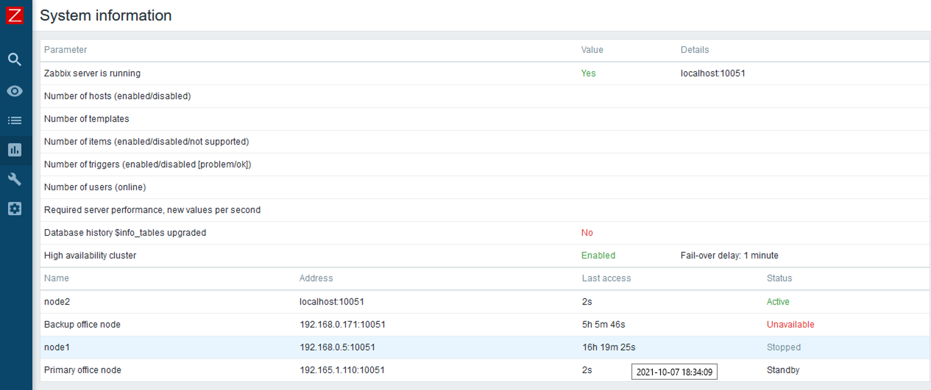
Zabbix server High Availability cluster

With the release of Zabbix 6.0 LTS, Zabbix administrators will now have the ability to deploy Zabbix server HA cluster out-of-the-box. No additional tools are required to achieve this.

Zabbix server HA cluster supports an unlimited number of Zabbix server nodes. All nodes will use the same database backend – this is where the status of all nodes will be stored in the ha_node table. Nodes will report their status every 5 seconds by updating the corresponding record in the ha_node table.

To enable High availability, you will first have to define a new parameter in the Zabbix server configuration file: HANodeName

  • Empty by default
  • This parameter should contain an arbitrary name of the HA node
  • Providing value to this parameter will enable Zabbix server cluster mode

Standby nodes monitor the last access time of the active node from the ha_node table.

  • If the difference between last access time and current time reaches the failover delay, the cluster fails over to the standby node
  • Failover operation is logged in the Zabbix server log

It is possible to define a custom failover delay – a time window after which an unreachable active node is considered lost and failover to one of the standby nodes takes place.

As for the Zabbix proxies, the Server parameter in the Zabbix proxy configuration file now supports multiple addresses separated by a semicolon. The proxy will attempt to connect to each of the nodes until it succeeds.

Other HA cluster related features:

  • New command-line options to check HA cluster status
  • hanode.get API method to obtain the list of HA nodes
  • The new internal check provides LLD information to discover Zabbix server HA nodes
  • HA Failover event logged in the Zabbix Audit log
  • Zabbix Frontend will automatically switch to the active Zabbix server node

You can find a more detailed look at the Zabbix Server HA cluster feature in the Zabbix Summit Online 2021 speech dedicated to the topic.

Business service monitoring

The Services section has received a complete redesign in Zabbix 6.0 LTS. Business Service Monitoring (BSM) enables Zabbix administrators to define services of varying complexity and monitor their status.

BSM provides added value in a multitude of use cases, where we wish to define and monitor services based on:

  • Server clusters
  • Services that utilize load balancing
  • Services that consist of a complex IT stack
  • Systems with redundant components in place
  • And more

Business Service monitoring has been designed with scalability in mind. Zabbix is capable of monitoring over 100k services on a single Zabbix instance.

For our Business Service example, we used a website, which depends on multiple components such as the network connection, DB backend, Application server, and more. We can see that the service status calculation is done by utilizing tags and deciding if the existing problems will affect the service based on the problem tags.

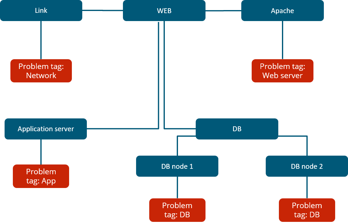
In Zabbix 6.0 LTS there are many ways how service status calculations can be performed. In case of a problem, the service state can be changed to:

  • The most critical problem severity, based on the child service problem severities
  • The most critical problem severity, based on the child service problem severities, only if all child services are in a problem state
  • The service is set to constantly be in an OK state

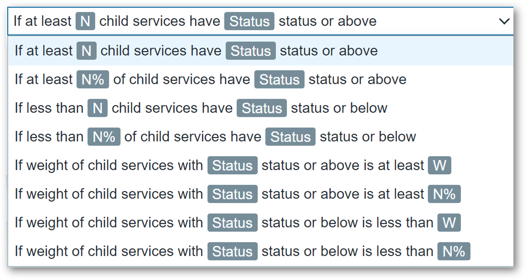
Changing the service status to a specific problem severity if:

  • At least N or N% of child services have a specific status
  • Define service weights and calculate the service status based on the service weights

There are many other additional features, all of which are covered in our Zabbix Summit Online 2021 speech dedicated to Business Service monitoring:

  • Ability to define permissions on specific services
  • SLA monitoring
  • Business Service root cause analysis
  • Receive alerts and react on Business Service status change
  • Define Business Service permissions for multi-tenant environments

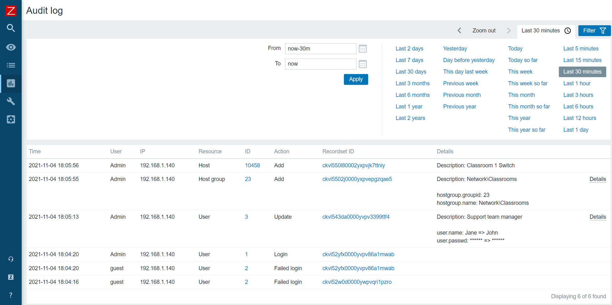
New Audit log schema

The existing audit log has been redesigned from scratch and now supports detailed logging for both Zabbix server and Zabbix frontend operations:

  • Zabbix 6.0 LTS introduces a new database structure for the Audit log
  • Collision resistant IDs (CUID) will be used for ID generation to prevent audit log row locks
  • Audit log records will be added in bulk SQL requests
  • Introducing Recordset ID column. This will help users recognize which changes have been made in a particular operation

The goal of the Zabbix 6.0 LTS audit log redesign is to provide reliable and detailed audit logging while minimizing the potential performance impact on large Zabbix instances:

  • Detailed logging of both Zabbix frontend and Zabbix server records
  • Designed with minimal performance impact in mind
  • Accessible via Zabbix API

Implementing the new audit log schema is an ongoing effort – further improvements will be done throughout the Zabbix update life cycle.

Machine learning

New trend functions have been added which utilize machine learning to perform anomaly detection and baseline monitoring:

  • New trend function – trendstl, allows you to detect anomalous metric behavior
  • New trend function – baselinewma, returns baseline by averaging data periods in seasons
  • New trend function – baselinedev, returns the number of standard deviations

An in-depth look into Machine learning in Zabbix 6.0 LTS is covered in our Zabbix Summit Online 2021 speech dedicated to machine learning, anomaly detection, and baseline monitoring.

New ways to visualize your data

Collecting and processing metrics is just a part of the monitoring equation. Visualization and the ability to display our infrastructure status in a single pane of glass are also vital to large environments. Zabbix 6.0 LTS adds multiple new visualization options while also improving the existing features.

  • The data table widget allows you to create a summary view for the related metric status on your hosts
  • The Top N and Bottom N functions of the data table widget allow you to have an overview of your highest or lowest item values
  • The single item widget allows you to display values for a single metric
  • Improvements to the existing vector graphs such as the ability to reference individual items and more
  • The SLA report widget displays the current SLA for services filtered by service tags

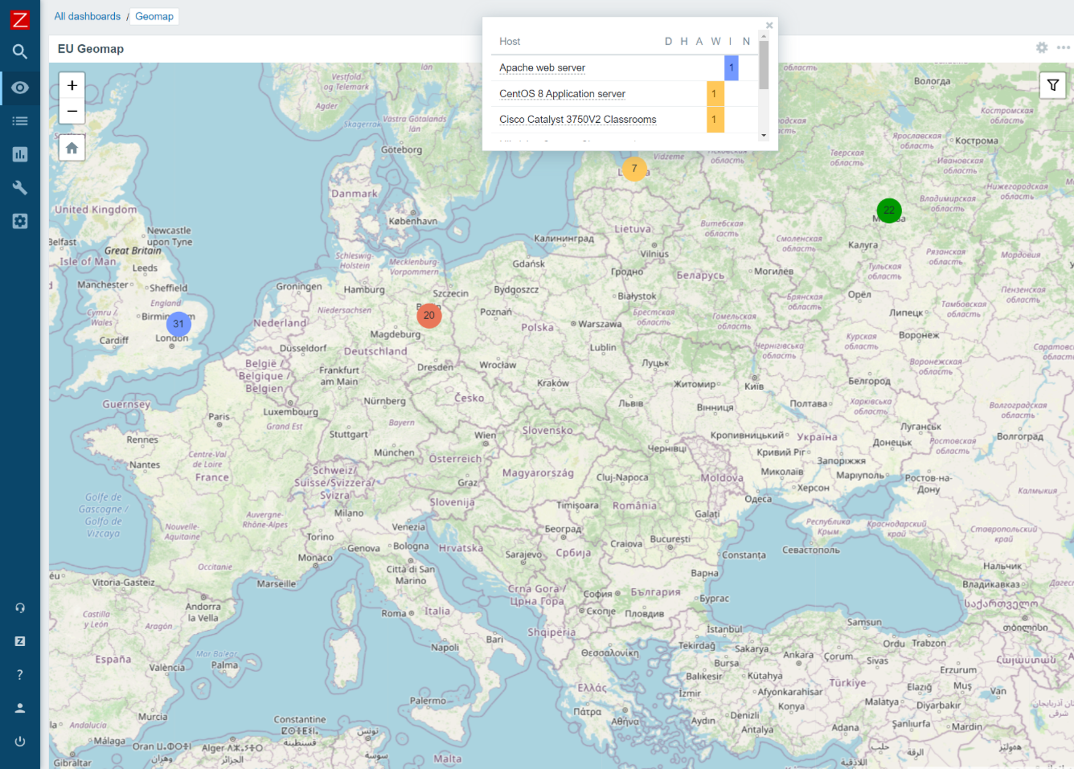
We are proud to announce that Zabbix 6.0 LTS will provide a native Geomap widget. Now you can take a look at the current status of your IT infrastructure on a geographic map:

  • The host coordinates are provided in the host inventory fields
  • Users will be able to filter the map by host groups and tags
  • Depending on the map zoom level – the hosts will be grouped into a single object
  • Support of multiple Geomap providers, such as OpenStreetMap, OpenTopoMap, Stamen Terrain, USGS US Topo, and others

Zabbix agent – improvements and new items

Zabbix agent and Zabbix agent 2 have also received some improvements. From new items to improved usability – both Zabbix agents are now more flexible than ever. The improvements include such features as:

  • New items to obtain additional file information such as file owner and file permissions
  • New item which can collect agent host metadata as a metric
  • New item with which you can count matching TCP/UDP sockets
  • It is now possible to natively monitor your SSL/TLS certificates with a new Zabbix agent2 item. The item can be used to validate a TLS/SSL certificate and provide you additional certificate details
  • User parameters can now be reloaded without having to restart the Zabbix agent

In addition, a major improvement to introducing new Zabbix agent 2 plugins has been made. Zabbix agent 2 now supports loading stand-alone plugins without having to recompile the Zabbix agent 2.

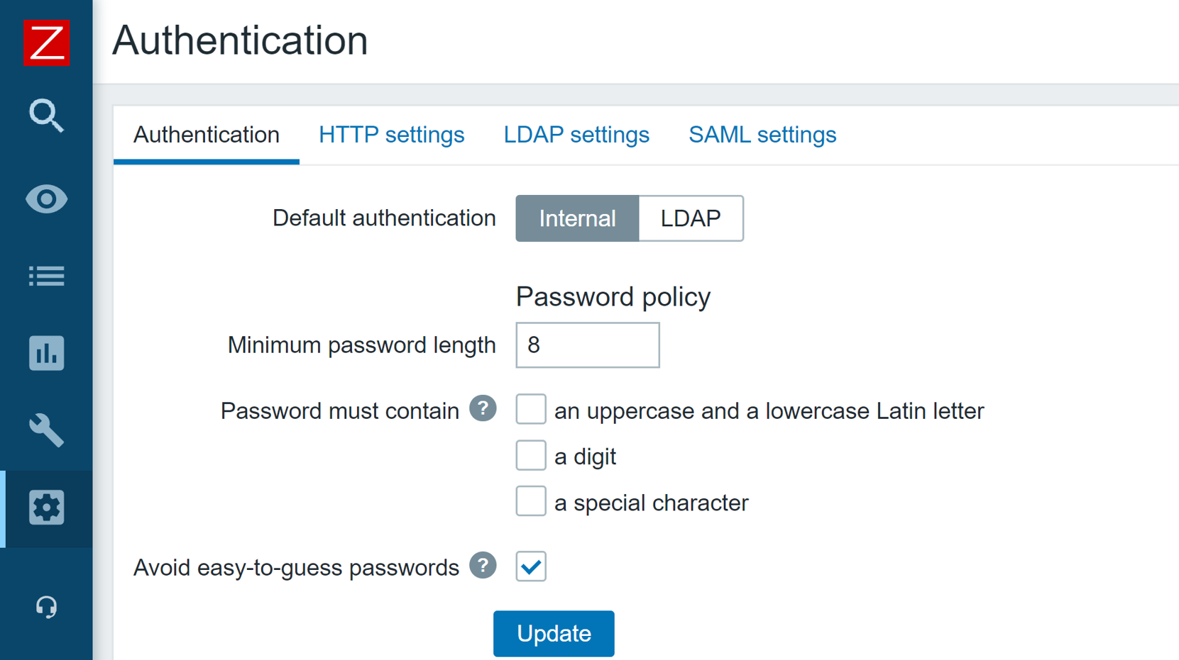
Custom Zabbix password complexity requirements

One of the main improvements to Zabbix security is the ability to define flexible password complexity requirements. Zabbix Super admins can now define the following password complexity requirements:

  • Set the minimum password length
  • Define password character requirements
  • Mitigate the risk of a dictionary attack by prohibiting the usage of the most common password strings

UI/UX improvements

Improving and simplifying the existing workflows is always a priority for every major Zabbix release. In Zabbix 6.0 LTS we’ve added many seemingly simple improvements, that have major impacts related to the “feel” of the product and can make your day-to-day workflows even smoother:

  • It is now possible to create hosts directly from MonitoringHosts
  • Removed MonitoringOverview section. For improved user experience, the trigger and data overview functionality can now be accessed only via dashboard widgets.
  • The default type of information for items will now be selected automatically depending on the item key.
  • The simple macros in map labels and graph names have been replaced with expression macros to ensure consistency with the new trigger expression syntax

New templates and integrations

Adding new official templates and integrations is an ongoing process and Zabbix 6.0 LTS is no exception here’s a preview for some of the new templates and integrations that you can expect in Zabbix 6.0 LTS:

  • f5 BIG-IP
  • Cisco ASAv
  • HPE ProLiant servers
  • Cloudflare
  • InfluxDB
  • Travis CI
  • Dell PowerEdge

Zabbix 6.0 also brings a new GitHub webhook integration which allows you to generate GitHub issues based on Zabbix events!

Other changes and improvements

But that’s not all! There are more features and improvements that await you in Zabbix 6.0 LTS. From overall performance improvements on specific Zabbix components, to brand new history functions and command-line tool parameters:

  • Detect continuous increase or decrease of values with new monotonic history functions
  • Added utf8mb4 as a supported MySQL character set and collation
  • Added the support of additional HTTP methods for webhooks
  • Timeout settings for Zabbix command-line tools
  • Performance improvements for Zabbix Server, Frontend, and Proxy

Questions and answers

Q: How can you configure geographical maps? Are they similar to regular maps?

A: Geomaps can be used as a Dashboard widget. First, you have to select a Geomap provider in the Administration – General – Geographical maps section. You can either use the pre-defined Geomap providers or define a custom one. Then, you need to make sure that the Location latitude and Location longitude fields are configured in the Inventory section of the hosts which you wish to display on your map. Once that is done, simply deploy a new Geomap widget, filter the required hosts and you’re all set. Geomaps are currently available in the latest alpha release, so you can get some hands-on experience right now.

Q: Any specific performance improvements that we can discuss at this point for Zabbix 6.0 LTS?

A: There have been quite a few. From the frontend side – we have improved the underlying queries that are related to linking new templates, therefore the template linkage performance has increased. This will be very noticeable in large instances, especially when linking or unlinking many templates in a single go.
There have also been improvements to Server – Proxy communication. Specifically – the logic of how proxy frees up uncompressed data. We’ve also introduced improvements on the DB backend side of things – from general improvements to existing queries/logic, to the introduction of primary keys for history tables, which we are still extensively testing at this point.

Q: Will you still be able to change the type of information manually, in case you have some advanced preprocessing rules?

A: In Zabbix 6.0 LTS Zabbix will try and automatically pick the corresponding type of information for your item. This is a great UX improvement since you don’t have to refer to the documentation every time you are defining a new item. And, yes, you will still be able to change the type of information manually – either because of preprocessing rules or if you’re simply doing some troubleshooting.

Tim Peake joins us as we get ready to launch special Raspberry Pi computers to space

Post Syndicated from Katie Gouskos original https://www.raspberrypi.org/blog/tim-peake-parents-stem-astro-pi-raspberry-pi-computers-space-launch/

We’re feeling nostalgic because six years ago, two special Raspberry Pi computers named Ed and Izzy were travelling to the International Space Station (ISS) from Cape Canaveral, Florida, USA. These two Astro Pi units joined British ESA astronaut Tim Peake as part of his six-month Principia space mission. Tim and Astro Pis Ed and Izzy helped hundreds of young people run their own computer programs in space as part of the first Astro Pi Challenge.

We are also feeling excited, because Tim and our Head of Youth Partnerships, Olympia Brown, are talking to British TV and radio shows today about all things space and Astro Pi, including the exciting new developments and how families can get involved! You might catch Tim on your favourite channel.

Tim Peake being interviewed about the Astro Pi Challenge and how parents getting their children involved will benefit the whole family.

Tim Peake has been our Astro Pi champion from the start

Tim says: “I had the privilege to take the first Astro Pi computers to the International Space Station in 2015. Since then, more than 50,000 children have run experiments and sent messages into orbit. The Astro Pi Challenge is a great activity for children and their parents to discover more about coding and to use digital tools to be creative.”

During his space mission, Tim Peake deployed Astro Pi units Ed and Izzy in a number of different locations on board the ISS. He was responsible for loading the Astro Pi participants’ programs onto Ed and Izzy, collecting the data they generated, and making sure it was downlinked back to Earth for the participants.

Tim Peake with one of the first two Astro Pi units during his Principia mission on the ISS.
Tim Peake with one of the first two Astro Pis unit during his Principia mission on the ISS

Fast forward six years, and we’re retiring Astro Pis Ed and Izzy and sending two upgraded Astro Pi units to space – in just over a week’s time, to be precise. This year, Italian ESA astronaut Samantha Cristoforetti will be taking the helm for the Challenge on board the ISS, while Tim continues to champion the Astro Pi Challenge down here on Earth.

Thank you Tim, for inspiring so many families to get involved with STEM and coding.

Your family’s very own space mission with Astro Pi

To get involved in the Astro Pi Challenge, you and your young people don’t even have to wait until the new Raspberry Pi computers arrive on the ISS. You can do Astro Pi Mission Zero — the beginners’ coding activity of the European Astro Pi Challenge — today!

Mission Zero participant Liz with her 2020-2021 certificate

In Mission Zero, young people, by themselves or in a team of up to four, follow our step-by-step instructions to write the code for a simple program, which we will send up to ISS to run on the new Astro Pi units. With their program, young people take a humidity reading on board the ISS and show it to the astronauts stationed there, together with a personal message or colourful design. This beginner-friendly coding activity takes about an hour and can be done on any computer in a web browser. It’s completely free too.

Logo of Mission Zero, part of the European Astro Pi Challenge.

As a parent (or educator), you support young people on Mission Zero by:

  • Registering as a Mission Zero mentor on astro-pi.org so we can send you a unique code for submitting your child’s program once it’s written
  • Helping them follow the step-by-step instructions so you can learn about coding together
  • Motivating them to keep going if their program doesn’t work right away, and helping to spot mistakes
  • Celebrating with them when they’ve finished writing the code for their Mission Zero program

After a young person’s Mission Zero code has run and their message has been shown in the ISS, we’ll send you a special certificate for them so you can commemorate their space mission.

A tweet about a young person who participated in Astro Pi Mission Zero.

And this year, Astro Pi Mission Zero is extra special: we are asking all participants to help us name the upgraded Raspberry Pi computers that will go to live on board the ISS. We’ve created a list of renowned European scientists whose names participants can vote for, in case you need inspiration.

Parents have lots of enthusiasm for learning about science and technology

It’s not just young people that benefit from getting involved with the Astro Pi Challenge – it’s something the whole family will enjoy doing together. And as findings from our recent UK survey showed, parents are rediscovering their passion for science, technology, and coding through helping their kids with homework. The survey found that parents of children in primary and secondary school are far more likely than any other group of adults to enjoy learning about science, with 3 in 5 parents (62%) revealing their enthusiasm for the subject. Nearly as many parents (58%) wished they had greater knowledge of STEM from school, and 62% said they are interested in learning how to code.

A mother and daughter do a coding activity together at a laptop at home.

“It’s wonderful to find out that parents of schoolchildren are discovering a passion for science and technology, especially after a year of home-schooling where they have been able to see first-hand what their children are learning.” says Olympia Brown, our Head of Youth Partnerships. “The Astro Pi Challenge is a fun, free, and creative way to learn about coding and carry out science experiments on board the International Space Station that both children and parents can get involved in.”

Young people love Astro Pi Mission Zero

If Tim Peake and we have not convinced you how fun and inspiring the Astro Pi Challenge will be for your family, then here are some young people to tell you about their experiences. We asked learners at Linton-on-Ouse Primary School how they found taking part in this year’s Mission Zero.

Learners at a Primary School taking part in Mission Zero.
Learners at Linton-on-Ouse Primary School taking part in Mission Zero

This is what some of the young learners shared with us:

“I learned a bit about how to code. Everyone was very helpful. This was very fun, and I wish we can do this again. It was tricky when we tried to make the colours change.”

– A learner in Year 4

“I worked as a team by helping check all the time. Next time I want to do it on my own, because I am feeling confident.”

– A learner in Year 3

Head over to astro-pi.org to register as a Mission Zero mentor today and start coding with your children. There you’ll find all the details you need for your family space mission.

The post Tim Peake joins us as we get ready to launch special Raspberry Pi computers to space appeared first on Raspberry Pi.

Configure alerts of high CPU usage in applications using Amazon OpenSearch Service anomaly detection: Part 1

Post Syndicated from Jey Vell original https://aws.amazon.com/blogs/big-data/part-1-configure-alerts-of-high-cpu-usage-in-applications-using-amazon-opensearch-service-anomaly-detection/

Amazon OpenSearch Service (successor to Amazon Elasticsearch Service) is a fully managed service that makes it easy to deploy, secure, and run Elasticsearch cost-effectively at scale. Amazon OpenSearch Service supports many use cases, including application monitoring, search, security information and event management (SIEM), and infrastructure monitoring. Amazon OpenSearch Service also offers a rich set of functionalities such as UltraWarm, fine-grained access control, alerting, and anomaly detection.

In this two-part post, we show you how to use anomaly detection in Amazon OpenSearch Service and configure alerts for high CPU usage in applications. In Part 1, we discuss how to set up your anomaly detector.

Solution overview

Anomaly detection in Amazon OpenSearch Service automatically detects anomalies in your Amazon OpenSearch Service data in near-real time by using the Random Cut Forest (RCF) algorithm. The RCF algorithm computes an anomaly grade and confidence score value for each incoming data point. Anomaly detection uses these values to differentiate an anomaly from normal variations in your data.

The following screenshot shows a sample anomaly history dashboard on the Amazon OpenSearch Service console.

You can configure anomaly detectors via the Amazon OpenSearch Service Kibana dashboard or API. The key elements for creating an anomaly detector are detector creation and model configuration. In the following steps, we create an anomaly detector for application log files with CPU usage data.

Create a detector

The first step in creating an anomaly detection solution is creating a detector. A detector is an individual anomaly detection task. You can have more than one detector, and they all can run simultaneously. To create your detector, complete the following steps:

  1. On the Anomaly detection dashboard inside your Kibana dashboard, choose Detectors.
  2. Choose Create detector.
  3. For Name, enter a unique name for your detector.
  4. For Description, enter an optional description.
  5. For Index, choose an index where you want to identify the anomaly.
  6. For Timestamp field, choose the timestamp field from your index.

Optionally, you can add a data filter. This data filter helps you analyze only a subset of your data source and reduce the noisy data.

  1. For Data filter, choose Visual editor.
  2. Choose your field, operator, and value.

Alternatively, choose Custom expression and add in your own filter query.

  1. Set the detector operation settings:
    1. Detector interval – This defines the time interval for the detector to collect the data. During this time, the detector aggregates the data, then feeds the aggregated results into the anomaly detection model. The number of data points depends on the interval value. A shorter interval time results in a smaller sample size. We recommend setting the interval based on actual data. Too long of an interval might delay the results, and too short might miss some data points.
    2. Window delay – This adds extra processing time to ensure that all data within the window is present.

Configure the model

In order to run the anomaly detection model, you must configure certain model parameters. One key parameter is feature selection. A feature is a field in the index that is monitored for anomalies using different aggregation methods. You can apply anomaly detection to more than one feature for the index specified in the detector’s data source. After you create the detector, you need to configure the model with the right features to enable anomaly detection.

  1. On the anomaly detection dashboard, under the detector name, choose Configure model.
  2. On the Edit model configuration page, for Feature name, enter a name.
  3. For Feature state, select Enable feature.
  4. For Find anomalies based on, choose Field value.
  5. For Aggregation method, choose your appropriate aggregation method.

For example, if you choose average(), the detector finds anomalies based on the average values of your feature. For this post, we choose sum().

  1. For Field, choose your field.

As of this writing, Amazon OpenSearch Service supports the category field for high cardinality. You can use the category field for keyword or IP field type. The category field categorizes or slices the source time series with a dimension like IP addresses, product SKUs, zip codes, and so on. This provides a granular view of anomalies within each entity of the category field, to help you isolate and debug issues. For example, the CPU usage percentage doesn’t help identify the specific instance causing the issue. But by using the host IP categorical value, you may able to find the specific host causing the anomaly.

  1. In the Category field, select Enable category field.
  2. For Field, choose your field.
  3. In the Advanced Settings section, for Window size, set the number of intervals to consider in a detection window.

We recommend choosing the window size value based on the actual data. If you expect missing values in your data or if you want the anomalies based on the current interval, choose 1. If your data is continuously ingested and you want the anomalies based on multiple intervals, choose a larger window size.

In the Sample anomaly history section, you can see a preview of the anomalies.

  1. Choose Save and start detector.
  2. In the pop-up window, select when to start the detector (automatically or manually).
  3. Choose Confirm.

Summary

This post explained the different steps required to create an anomaly detector with Amazon OpenSearch Service. You can use anomaly detection for many use cases, including finding anomalies in access logs from different services, using clickstream data, using IP address data, and more.

Amazon OpenSearch Service anomaly detection is available on domains running any OpenSearch version or Elasticsearch 7.4 or later. All instance types support anomaly detection, except for t2.micro and t2.small.

In the next part of this post, we cover how to set up an alert for these anomalies using the Amazon OpenSearch Service alerting feature.


About the Authors

Jey Vell is a Senior Solutions Architect with AWS, based in Austin TX. Jey specializes in Analytics and ML/AI. Jey works closely with Amazon OpenSearch Service team, providing architecture guidance and technical support to the AWS customers with their search workloads. He brings to his role over 20 years of technology experience in software development and architecture, and IT management.

Jon Handler is a Senior Principal Solutions Architect, specializing in AWS search technologies – Amazon CloudSearch, and Amazon OpenSearch Service. Based in Palo Alto, he helps a broad range of customers get their search and log analytics workloads deployed right and functioning well.

Privacy video: Innovating securely

Post Syndicated from Chad Woolf original https://aws.amazon.com/blogs/security/privacy-video-innovating-securely/

I’m pleased to share a video of a conversation about privacy I had with my colleague Laura Dawson, the North American Lead at the AWS Institute. Privacy is becoming more of a strategic issue for our customers, similar to how security is today. We discussed how, while the two topics are similar in some ways, they also have important differences. We also talked about the importance of building a strong privacy program, and how AWS helps customers safeguard privacy while still taking advantage of digital modernization opportunities.

The differences between security and privacy aren’t fully understood in some industries. Security principles are better known in the industry – security involves considering the confidentiality, integrity, and availability of information. It’s about keeping unauthorized parties away from your data, and about making sure access to your systems and data is appropriate. Similarly, privacy is about control of data through its entire lifecycle, specifically personal identifiable information (PII). That includes the collection, use, transmission, and deletion of that data. Properly managing the privacy of PII is like security when you consider the “access control” aspect, but privacy is about making sure you always have granular control of what is happening to that PII from formation/gathering through to deletion.

Unlike security, which is now commonly recognized as a core business function, privacy practices and principles are still in the early stages of being widely accepted. This is why AWS advocates for organizations to follow the principles of Privacy by Design, to ensure that privacy processes and controls are baked into everything you do.

I also discussed with Laura some of the privacy trends I see happening in the tech industry right now, such as homomorphic encryption, anonymization, and PII discovery tools. The privacy challenges organizations face today, however, aren’t just technology challenges; they’re also business challenges, of how to get value from the data you control, in a way that meets privacy best practices and accounts for your customers’ interests.

For more about these and other privacy topics, check out the video of my conversation with Laura. To learn more about privacy at AWS, check out the Data Privacy Center and Data Protection at AWS.

Author

Chad Woolf

Chad joined Amazon in 2010 and built the AWS compliance functions from the ground up, including audit and certifications, privacy, contract compliance, control automation engineering and security process monitoring. Chad’s work also includes enabling public sector and regulated industry adoption of the AWS cloud and leads the AWS trade and product compliance team.

Haas: Surviving Without A Superuser – Part One

Post Syndicated from original https://lwn.net/Articles/878206/rss

PostgreSQL developer Robert Haas has begun
a blog series
on what would be needed to allow database administrators
to safely delegate superuser powers.

Consider, for example, the case of a service provider who would
like to support a database with multiple customers as tenants. The
customers will naturally want to feel as if they have the powers of
a true superuser, with the ability to do things like create new
roles, drop old ones, change permissions on objects that they don’t
own, and generally enjoy the freedom to bypass permission checks at
the SQL level which superusers enjoy. The service provider, who is
the true superuser, also wants this, but does not want the
customers to be able to do the really scary things that a superuser
can do, like changing archive_command to
rm -rf / or deleting the
entire contents of pg_proc so that the system crashes and the
database in which the operation was performed is permanently
ruined.

Load CDC data by table and shape using Amazon Kinesis Data Firehose Dynamic Partitioning

Post Syndicated from Anand Shah original https://aws.amazon.com/blogs/big-data/load-cdc-data-by-table-and-shape-using-amazon-kinesis-data-firehose-dynamic-partitioning/

Amazon Kinesis Data Firehose is the easiest way to reliably load streaming data into data lakes, data stores, and analytics services. Customers already use Amazon Kinesis Data Firehose to ingest raw data from various data sources using direct API call or by integrating Kinesis Data Firehose with Amazon Kinesis Data Streams including “change data capture” (CDC) use case.

Customers typically use single Kinesis Data Stream per business domain to ingest CDC data. For example, related fact and dimension tables change data is sent to the same stream. Once the data is loaded to Amazon S3, customers use ETL tools to split the data by tables, shape, and desired partitions as the first step in the data enrichment process.

This post demonstrates how customers can use Amazon Kinesis Firehose Dynamic Partitioning to split the data by table, shape (by message schema/version), and by desired partitions on the fly to do this first step of data enrichment while ingesting data.

Solution Overview

In this post, we provide a working example of a CDC pipeline where fake customer, order, and transaction table data is pushed from the source and registered as tables to the AWS Glue Data Catalog. The following architecture diagram illustrates this overall flow. We are using AWS Lambda to generate test CDC data for this post. However, in the real world you would use AWS Data Migration Service (DMS) or a similar tool to push change data to the Amazon Kinesis Data Stream.

The workflow includes the following steps:

  1. An Amazon EventBridge event triggers an AWS Lambda function every minute.
  2. The Lambda function generates test transactions, customers and order CDC data, as well as sends the data to Amazon Kinesis Data Stream.
  3. Amazon Kinesis Data Firehose reads data from Amazon Kinesis Data Stream.
  4. Amazon Kinesis Data Firehose
    1. Applies Dynamic Partitioning configuration defined in the Firehose configuration
    2. Invokes AWS Lambda transform to derive custom Dynamic Partitioning.
  5. Amazon Kinesis Data Firehose saves data to Amazon Simple Storage Service (S3) bucket.
  6. The user runs queries on Amazon S3 bucket data using Amazon Athena, which internally uses the AWS Glue Data Catalog to supply meta data.

Deploying using AWS CloudFormation

You use CloudFormation templates to create all of the necessary resources for the data pipeline. This removes opportunities for manual error, increases efficiency, and ensures consistent configurations over time.

Steps to follow:

  1. Click here to Launch Stack:
  2. Acknowledge that the template may create AWS Identity and Access Management (IAM) resources.
  3. Choose Create stack.

This CloudFormation template takes about five minutes to complete and creates the following resources in your AWS account:

  • An S3 bucket to store ingested data
  • Lambda function to publish test data
  • Kinesis Data Stream connected to Kinesis Data Firehose
  • A Lambda function to compute custom dynamic partition for Kinesis Data Firehose transform
  • AWS Glue Data Catalog tables and Athena named queries for you to query data processed by this example

Once the AWS CloudFormation stack creation is successful, you should be able to see data automatically arriving to Amazon S3 in about five more minutes.

Data sources input

The Lambda function automatically publishes four types of messages to the Kinesis Data Stream at regular intervals with random data when invoked in the following format. In this example, we use three tables:

  • Customers: Has basic customer details.
  • Orders: Mimics orders placed by customers on the shopping website or mobile app.
  • Transactions: Mimics payment transaction done for the order. The transaction table showcases possible message schema evolution that can happen over time from message schema v1 to v2. It also shows how you can split messages by schema version if you don’t want to merge them into a universal schema.

Customer table sample message

{
   "version": 1,
   "table": "Customer",
   "data": {
        "id": 1,
        "name": "John",
        "country": "US"
   }
}

Orders table sample message

{
   "version": 1,
   "table": "Order",
   "data": {
        "id": 1,
        "customerId": 1,
        "qty": 1,
        "product": {
            "name": "Book 54",
            "price": 12.6265
        }
   }
}

Transactions in old message format (v1)

{
    "version": 1, 
    "txid": "52", 
    "amount": 32.6516
}

Transactions in new message format (v2 – latest)

This message example demonstrates message evolution over time. txid from old message format is now renamed to transactionId, and new information like source is added to the original old transaction message in the new message version v2.

{
   "version": 2,
   "transactionId": "52",
   "amount": 32.6516,
   "source": "Web"
}

Dynamic Partitioning Logic

Amazon Kinesis Data Firehose dynamic partitioning configuration is defined using jq style syntax. We will use the table field for the first partition and the version field for the second level partition. We can derive the table partition using dynamic partitioning jq syntax “.version”. As you can see, the version field is available in all of the messages. Therefore, we can use it directly in partitioning. However, the table field is not available for old and new transaction messages. Therefore, we derive the table field using custom transform Lambda function.

We check the existence of the table field from the incoming message and populate it with the static value “Transaction” if table field is not present. Lambda function also returns PartitionKeys for Kinesis Data Firehose to use as dynamic partition. The Lambda function also derives the year, month, and day from the current time.

for firehose_record_input in firehose_records_input['records']:
    # Get user payload
    payload = base64.b64decode(firehose_record_input['data'])
    json_value = json.loads(payload)


    # Create output Firehose record and add modified payload and record ID to it.
    firehose_record_output = {}

    table = "Transaction"
    if "table" in json_value:
        table = json_value["table"]

    now = datetime.datetime.now()
    partition_keys = {"table": table, "year": str(now.year), "month": str(now.month), "day": str(now.day)}

The Kinesis Data Firehose S3 destination Prefix is set to table=!{partitionKeyFromLambda:table}/version=!{partitionKeyFromQuery:version}/year=!{partitionKeyFromLambda:year}/month=!{partitionKeyFromLambda:month}/day=!{partitionKeyFromLambda:day}/

  • table partition key is coming from the Lambda function based on custom logic.
  • version partition key is extracted using jq expression using Kinesis Data Firehose dynamic partition configuration. Here, the version refers to the shape of the message and not the version of the data. For example, Updates to Customer record with same ID is not merged into one.
  • year, month, and day partition keys are coming from the Lambda function based on current time

You can follow the respective links from the CloudFormation stack Output tab to deep dive into the Kinesis Data Firehose configuration, record transformer Lambda function source code, and see output files in the Amazon S3 curated bucket. The entire code is also available in the GitHub repository.

Ingested data output

Kinesis Data Firehose processes all the messages and outputs result in the following S3 hive style partitioned paths:

# AWS Glue Data Catalog table transactions_v1
s3://curated-bucket/table=transaction/version=1/year=2021/month=9/day=20/file-name.gz
# AWS Glue Data Catalog table transactions
s3://curated-bucket/table=transaction/version=2/year=2021/month=9/day=20/file-name.gz
# AWS Glue Data Catalog table customers
s3://curated-bucket/table=customer/version=1/year=2021/month=9/day=20/file-name.gz
# Glue catalog table orders
s3://curated-bucket/table=order/version=1/year=2021/month=9/day=20/file-name.gz

Query output data stored in Amazon S3

Kinesis Data Firehose loads new data every minute to the Amazon S3 bucket, and the associated tables are already created by CloudFormation for you in the AWS Glue Data Catalog. You can directly query Amazon S3 bucket data using the following steps:

  1. Go to Amazon Athena service and select the database with the same name as the CloudFormation stack name without dashes.
  2. Select the three dots next to each table name to open the table menu and select Load Partitions. This will add a new partition to the AWS Glue Data Catalog.
  3. Go to the CloudFormation stack Output tab.
  4. Select the link mentioned next to the key AthenaQueries.
  5. This will take you to the Amazon Athena saved query console. Type the word Blog to search named queries created by this blog.
  6. Select the query called “Blog – Query Customer Orders”. This will open the query in the Athena query console. Select Run query to see the results.
  7. Select the Saved queries menu from the top bar to go back to the Amazon Athena saved query console. Repeat the steps for other Blog queries to see results from the “new and old transactions” queries.

Clean up

Complete the following steps to delete your resources and stop incurring costs:

  1. Go to the CloudFormation stack Output tab.
  2. Select the link mentioned next to the key PauseDataSource. This will take you to the Amazon EventBridge event rules console.
  3. Select the Actions button from the top right menu bar and select Disable.
  4. Confirm the choice by clicking the Disable button again on the prompt. This will disable Amazon EventBridge event trigger that invokes the data generator Lambda function. This lets us make sure that no new data is sent to the Kinesis data stream by Lambda from now onward.
  5. Wait for at least two minutes for all of the buffered events to reach to the S3 from the Kinesis Data Firehose.
  6. Go back to the CloudFormation stack Output tab.
  7. Select the link mentioned next to the key S3BucketCleanup.

You’re redirected to the Amazon S3 console.

  1. Enter permanently delete to delete all of the objects in your S3 bucket.
  2. Choose Empty.
  3. On the AWS CloudFormation console, select the stack you created and choose Delete.

Summary

This post demonstrates how to use the Kinesis Data Firehose Dynamic Partitioning feature to load CDC data on the fly in near real-time. It also shows how we can split CDC data by table and message schema version for backward compatibility and quick query capability. To learn more about dynamic partitioning, you can refer to this blog and this documentation. Provide us with any feedback you have about the new feature.


About the Author

Anand Shah is a Big Data Prototyping Solution Architect at AWS. He works with AWS customers and their engineering teams to build prototypes using AWS Analytics services and purpose-built databases. Anand helps customers solve the most challenging problems using the art of the possible technology. He enjoys beaches in his leisure time.

SEEK Asia modernizes search with CI/CD and Amazon OpenSearch Service

Post Syndicated from Fabian Tan original https://aws.amazon.com/blogs/big-data/seek-asia-modernizes-search-with-ci-cd-and-amazon-opensearch-service/

This post was written in collaboration with Abdulsalam Alshallah (Salam), Software Architect, and Hans Roessler, Principal Software Engineer at SEEK Asia.

SEEK is a market leader in online employment marketplaces with deep and rich insights into the future of work. As a global business, SEEK has a presence in Australia, New Zealand, Hong Kong, Southeast Asia, Brazil and Mexico and its websites attract over 400 million visits per year. SEEK Asia’s business operates across seven countries and includes leading portal brands such as jobsdb.com and jobstreet.com and leverages data and technology to create innovative solutions for candidates and hirers.

In this post, we share how SEEK Asia modernized their search-based system with a continuous integration and continuous delivery (CI/CD) pipeline and Amazon OpenSearch Service (successor to Amazon Elasticsearch Service).

Challenges associated with a self-managed search system

SEEK Asia provides a search-based system that enables employers to manage interactions between hirers and candidates. Although the system was already on AWS, it was a self-managed system running on Amazon Elastic Compute Cloud (Amazon EC2) with limited automation.

The self-managed system posed several challenges:

  • Slower release cycles – Deploying new configurations or new field mappings into the Elasticsearch cluster was a high-risk activity because changes affected the stability of the system. The little automation on both the self-managed cluster and workflows led to slower release cycles.
  • Higher operational overhead – Sizing the cluster to deliver greater performance, while managing cost effectively, was the other challenge. As with every other distributed system, even with sizing guidance, identifying the appropriate number of shards per node and the number of nodes to meet performance requirements still required some amount of trial and error, turning the exercise into a tedious and time-consuming activity. This consequently also led to slower release cycles. To overcome this challenge, in many occasions, oversizing the cluster became the quickest way to achieve the desired time to market, at the expense of cost.

Further challenges the team faced with self-managing their own Elasticsearch cluster included keeping up with new security patches, and minor and major platform upgrades.

Automating search delivery with Amazon OpenSearch Service

SEEK Asia knew that automation would the key to solving the challenges of their existing search service. Automating the undifferentiated heavy lifting would enable them to deliver more value to their customers quickly and improve staff productivity.

With the problems defined, the team set out to solve the challenges by automating the following:

  • Search infrastructure deployment
  • Search A/B testing infrastructure deployment
  • Redeployment of search infrastructure for any new infrastructure configuration (such as security patches or platform upgrades) and index mapping updates

The key services enabling the automation would be Amazon OpenSearch Service and establishing a search infrastructure CI/CD pipeline.

Architecture overview

The following diagram illustrates the architecture of the SEEK infrastructure and CI/CD pipeline with Amazon OpenSearch Service.

The workflow includes the following steps:

  1. Before the workflow kicks off, an existing Amazon OpenSearch Service cluster with a live feeder hydrates it. The live feeder is a serverless application built on Amazon Simple Queue Service (Amazon SQS) via Amazon Simple Notification Service (Amazon SNS) and AWS Lambda. Amazon SQS queues documents for processing, Amazon SNS enables data fanout (if required), and a Lambda function is invoked to process messages in the SQS queue to import data into Amazon OpenSearch Service. The feeder receives live updates for changes that need to be reflected on the cluster. Write concurrency to Amazon OpenSearch Service is managed by limiting the number of concurrent Lambda function invocations.
  2. The Amazon OpenSearch Service index mapping is version controlled in SEEK’s Git repository. Whenever an update to the index mapping is committed, the CI/CD pipeline kicks off a new Amazon OpenSearch Service cluster provisioning workflow.
  3. As part of the workflow, a new data hydration initialization feeder is deployed. The initialization feeder construct is similar to the live feeder, with one additional component: a script that runs within the CI/CD pipeline to calculate the number of batches required to hydrate the newly provisioned Amazon OpenSearch Service cluster up to a specific timestamp. The feeder systems were designed to achieve idempotency processing. This meant unique identifiers (UIDs) from the source data stores are reused for each document, and duplicated documents update an existing document with the exact same values.
  4. At the same time as Step 3, an Amazon OpenSearch Service cluster is deployed. To accelerate the initial data hydration process temporarily, the new cluster may be sized two or three times larger against sizing guidance with shard replicas and index refresh interval disabled until the hydration process is complete. The existing Amazon OpenSearch Service cluster remains as is, which means that two clusters are running concurrently.
  5. The script inspects the number of documents the source data store has and groups the documents by batch sizes. SEEK identified that 1,000 documents per batch provided the optimal ingestion import time, after running numerous experiments.
  6. Each batch is represented as one message and is queued into Amazon SQS via Amazon SNS. Every message that lands in Amazon SQS invokes a Lambda function. The Lambda function queries a separate data store, builds the document, and loads it into Amazon OpenSearch Service. The more messages that go into the queue, the more functions are invoked. To create baselines that allowed for further indexing optimization, the team took the following configurations into consideration and reiterated to achieve higher ingestion performance:
    1. Memory of the Lambda function
    2. Size of batch
    3. Size of each document in the batch
    4. Size of cluster (memory, vCPU, and number of primary shards)
  7. With the initialization feeder running, new documents are streamed to the cluster until it is synced with the data source. Eventually, the newly provisioned Amazon OpenSearch Service cluster catches up and is in the same state as the existing cluster. The hydration is complete when there are no remaining messages in the SQS queue.
  8. The initialization feeder is deleted and the Amazon OpenSearch Service cluster is downsized automatically to complete the deployment workflow, with replica shards created and the index refresh interval configured.
  9. Live search traffic is routed to the newly provisioned cluster when A/B testing is enabled via the API layer built on Application Load Balancer, Amazon Elastic Container Service (Amazon ECS), and Amazon CloudFront. The API layer decouples the client interface from the backend implementation that runs on Amazon OpenSearch Service.

Improved time to market and other outcomes

With Amazon OpenSearch Service, SEEK was able to automate an entire cluster, complete with Kibana, in a secure, managed environment. If testing didn’t produce the desired results, the team could change the dimensions of the cluster horizontally or vertically using different instance offerings within minutes. This enabled them to perform stress tests quickly to identify the sweet spot between performance and cost of the workload.

“By integrating Amazon OpenSearch Service with our existing CI/CD tools, we’re able to fully automate our search function deployments, which accelerated software delivery time,” says Abdulsalam Alshallah, APAC Software Architect. “The newly found confidence in the modern stack, alongside improved engineering practices, allowed us to mitigate the risk of changes—improving our time to market by 89% with zero impact to uptime.”

With the adoption of Amazon OpenSearch Service, other teams also saw improvements, including the following:

  • Common Vulnerability and Exposure (CVE) has dropped to zero with Amazon OpenSearch Service handling the underlying hardware security updates on SEEK’s behalf, improving their security posture
  • Improved availability with the Amazon OpenSearch Service Availability Zone awareness feature

Conclusion

Amazon OpenSearch Service managed capabilities has helped SEEK Asia to improve customer experience with speed and automation. By removing the undifferentiated heavy lifting, teams can deploy changes quickly to their search engines, allowing customers to get the latest search features faster and ultimately contributing to the SEEK purpose of helping people live more productive working lives and organisations succeed.

To learn more about Amazon OpenSearch Service, see Amazon OpenSearch Service features, the Developer Guide, or Introducing OpenSearch.


About the Authors

Fabian Tan is a Principal Solutions Architect at Amazon Web Services. He has a strong passion for software development, databases, data analytics and machine learning. He works closely with the Malaysian developer community to help them bring their ideas to life.

Hans Roessler is a Principal Software Architect at SEEKAsia. He is excited about new technologies and upgrading legacy to newer stacks. Always staying in touch with the latest technologies is one of his passions.

Abdulsalam Alshallah (Salam) is a Software architect at SEEK, Previously a Lead Cloud Architect for SEEKAsia, Salam has always been excited about new technologies, Cloud, Serverless & DevOps, in addition to his passion of eliminating wasted time/effort & resources; He is also one of the leaders of AWS User Group Malaysia.

Introducing stack graphs

Post Syndicated from Douglas Creager original https://github.blog/2021-12-09-introducing-stack-graphs/

Today, we announced the general availability of precise code navigation for all public and private Python repositories on GitHub.com. Precise code navigation is powered by stack graphs, a new open source framework we’ve created that lets you define the name binding rules for a programming language using a declarative, domain-specific language (DSL). With stack graphs, we can generate code navigation data for a repository without requiring any configuration from the repository owner, and without tapping into a build process or other CI job. In this post, I’ll dig into how stack graphs work, and how they achieve these results.

(This post is a condensed version of a talk that I gave at Strange Loop in October 2021. Please check out the video of that talk if you’d like to learn even more!)

What is code navigation?

Code navigation is a family of features that let you explore the relationships in your code and its dependencies at a deep level. The most basic code navigation features are “jump to definition” and “find all references.” Both build on the fact that names are pervasive in the code that we write. Programming languages let us define things — functions, classes, modules, methods, variables, and more. Those things have names so that we can refer back to them in other parts of our code.

A picture (even a simple one) is worth a thousand words:

a simple Python module

In this Python module, the reference to broil at the end of the file refers to the function definition earlier in the file. (Throughout this post, I’ll highlight definitions in red and references in blue.)

Our goal, then, is to collect information about the lists of definitions and references, and to be able to determine which definitions each reference maps to, for all of the code hosted on GitHub.

Why is this hard?

In the above example, the definition and reference were close to each other, and it was easy to visually see the relationship between them. But it won’t always be that easy!

names can shadow each other in Python but not in Rust

For instance, what if there are multiple definitions with the same name? In Python, names can shadow each other, which means that the broil reference should refer to the latter of the two definitions.

But these rules are language-specific! In Rust, top-level definitions are not allowed to shadow each other, but local variables are. So, this transliteration of my example from Python to Rust is an error according to the Rust language spec. If we were writing a Rust compiler, we would want to surface this error for the programmer to fix. But what about for an exploration feature like code navigation? We might want to show some result even for erroneous code. We’re only human, after all!

code can live in multiple packages

Up to now, I’ve only shown you examples consisting of a single file. But when was the last time you worked on a software project consisting of a single file? It’s much more likely that your code will be split across multiple files, multiple packages, and multiple repositories. Programming languages give us the ability to refer to definitions that might be quite far away. But as you might expect, the rules for how you refer to things in other files are different for different languages.

In the above example, I’ve split everything up into three files living in two separate packages or repositories. (I’m using emoji to represent the package names.) In Python, import statements let us refer to names defined in other modules, and the name of a module is determined by the name of the file containing its code. Together, this lets us see that the broil reference in chef.py in the “chef” package refers to the broil definition in stove.py in the “frying pan” package.

code can change

Code changes and evolves over time. What happens when one of your dependencies changes the implementation of a function that you’re calling? Here, the maintainers of the “frying pan” package have added some logging to the broil function. As a result, the broil reference in chef.py now refers to a different definition. Insidiously, it was an intermediate file that changed — not the file containing the reference, nor the file containing the original definition! If we’re not careful, we’ll have to reanalyze every file in the repository, and in all its dependencies, whenever any file changes! This makes the amount of work we must do quadratic in the number of changed files, rather than linear, which is especially problematic at GitHub’s scale.

Our last difficulty is one of scale. As mentioned above, we want to provide this feature for all of the code hosted on GitHub. Moreover, we don’t want to require any manual configuration on the part of each repository owner. You shouldn’t have to figure out how to produce code navigation data for your language and project, or have to configure a CI build to generate that data. Code navigation should Just Work.

At GitHub’s scale, this poses two problems. The first is the sheer amount of code that comes in every minute of every day. In each commit that we receive, it’s very likely that only a small number of files have been modified. We must be able to rely on incremental processing and storage, reusing the results that we’ve already calculated and saved for the files that haven’t changed.

The second challenge is the number of programming languages that we need to (eventually) support. GitHub hosts code written in every programming language imaginable. Git itself doesn’t care what language you use for your project — to Git, everything is just bytes. But for a feature like code navigation, where the name binding rules are different for each language, we must know how to parse and interpret the content of those files. To support this at scale, it must be as easy as possible for GitHub engineers and external language communities to describe the name binding rules for a language.

To summarize:

  • Different languages have different name binding rules.
  • Some of those rules can be quite complex.
  • The result might depend on intermediate files.
  • We don’t want to require manual per-repository configuration.
  • We need incremental processing to handle our scale.

Stack graphs

After examining the problem space, we created stack graphs to tackle these challenges, based on the scope graphs framework from Eelco Visser’s research group at TU Delft. Below I’ll discuss what stack graphs are and how they work.

Because we must rely on incremental results, it’s important that at index time (that is, when we receive pushes containing new commits), we look at each file completely in isolation. Our goal is to extract “facts” about each file that describe the definitions and references in the file, and all possible things that each reference could resolve to.

For instance, consider this example:

two Python files

Our final result must be able to encode the fact that the broil reference and definition live in different files. But to be incremental, our analysis must look at each file separately. I’m going to step into each file to show you what information GitHub can extract in isolation.

the stack graph for stove.py

Looking first at stove.py, we can see that it contains a definition of broil. From the name of the file, we know that this definition lives in a module called stove, giving a fully qualified name of stove.broil. We can create a graph structure representing this fact (along with information about the other symbols in the file). Each definition (including the module itself) gets a red, double-bordered definition node. The other nodes, and the pattern of how we’ve connected these nodes with edges, define the scoping and shadowing rules for these symbols. For other programming languages, which don’t implement the same shadowing behavior as Python, we’d use a different pattern of edges to connect everything.

the stack graph for kitchen.py

We can do the same thing for kitchen.py. The broil reference is represented by a blue, single-bordered reference node. The import statement also appears in the graph, as a gadget of nodes involving the broil and stove symbols.

Because we are looking at this file in isolation, we don’t yet know what the broil reference resolves to. The import statement means that it might resolve to stove.broil, defined in some other file — but that depends on whether there is a file defining that symbol. This example does in fact contain such a file (we just looked at it!), but we must ignore that while extracting incremental facts about kitchen.py.

At query time, however, we’re able to bring together the data from all files in the commit that you’re looking at. We can load the graphs for each of the files, producing a single “merged” graph for the entire commit:

the merged stack graph

Within this merged graph, every valid name binding is represented by a path from a reference node to a definition node.

However, not every path in the graph represents a valid name binding! For instance, looking only at the graph structure, there are perfectly fine paths from the broil reference node to the saute and bake definition nodes. To rule out those paths, we also maintain a symbol stack while searching for paths. Each blue node pushes a symbol onto the stack, and each red node pops a symbol from the stack. Importantly, we are not allowed to move into a “pop” node if its symbol does not match the top of the stack.

We’ve shown the contents of the symbol stack at a handful of places in the path that’s highlighted above. Most importantly, when we reach the portion of the graph containing the saute, broil, and bake definition nodes, the symbol stack contains ⟨broil⟩, ensuring that the only valid path that we discover is the one that ends at the broil definition.

We can also use different graph structures to handle my other examples. For example:

the stack graph for shadowed Python definitions

In this graph, we annotate some of the graph edges with a precedence value. Paths that include edges with a higher precedence value are preferred over those with lower precedences. This lets us correctly handle Python’s shadowing behavior.

For other programming languages, which don’t implement the same shadowing behavior as Python, we’d use a different pattern of edges to connect everything. For instance, the stack graph for my Rust example from earlier would be:

the stack graph for conflicting Rust definitions

To model Rust’s rule that top-level definitions with the same name are conflicts, we have a single node that all definitions hang off of. We can use precedences to choose whether to show all conflicting definitions (by giving them all the same precedence value), or just the first one (by assigning precedences sequentially).

With a stack graph available to us, we can implement “jump to definition:”

  1. The user clicks on a reference.
  2. We load in the stack graphs for each file in the commit, and merge them
    together.
  3. We perform a path-finding search starting from the reference node
    corresponding to the symbol that the user clicked on, considering
    symbol stacks and precedences to ensure that we don’t create any invalid
    paths.
  4. Any valid paths that we find represent the definitions that the reference
    refers to. We display those in a hover card.

Creating stack graphs using Tree-sitter

I’ve described how to use stack graphs to perform code navigation lookups, but I haven’t mentioned how to create stack graphs from the source code that you push to GitHub.

For that, we turned to Tree-sitter, an open source parsing framework. The Tree-sitter community has already written parsers for a wide variety of programming languages, and we already use Tree-sitter in many places across GitHub. This makes it a natural choice to build stack graphs on.

Tree-sitter’s parsers already let us efficiently parse the code that our users upload. For instance, the Tree-sitter parser for Python produces a concrete syntax tree (CST) for our stove.py example file:

$ tree-sitter parse stove.py
(module [0, 0] - [10, 0]
  (function_definition [0, 0] - [1, 8]
    name: (identifier [0, 4] - [0, 8])
    parameters: (parameters [0, 8] - [0, 10])
    body: (block [1, 4] - [1, 8]
      (pass_statement [1, 4] - [1, 8])))
  (function_definition [3, 0] - [4, 8]
    name: (identifier [3, 4] - [3, 9])
    parameters: (parameters [3, 9] - [3, 11])
    body: (block [4, 4] - [4, 8]
      (pass_statement [4, 4] - [4, 8])))
  (function_definition [6, 0] - [7, 8]
    name: (identifier [6, 4] - [6, 9])
    parameters: (parameters [6, 9] - [6, 11])
    body: (block [7, 4] - [7, 8]
      (pass_statement [7, 4] - [7, 8]))))

Tree-sitter also provides a query language that lets us look for patterns within the CST:

(function_definition
  name: (identifier) @name) @function

This query would locate all three of our example method definitions, annotating each definition as a whole with a @function label and the name of each method with a @name label.

As part of developing stack graphs, we’ve added a new graph construction language to Tree-sitter, which lets you construct arbitrary graph structures (including but not limited to stack graphs) from parsed CSTs. You use stanzas to define the gadget of graph nodes and edges that should be created for each occurrence of a Tree-sitter query, and how the newly created nodes and edges should connect to graph content that you’ve already created elsewhere. For instance, the following snippet would create the stack graph definition node for my example Python method definitions:

(function_definition
  name: (identifier) @name) @function
{
    node @function.def
    attr (@function.def) kind = "definition"
    attr (@function.def) symbol = @name
    edge @function.containing_scope -> @function.def
}

This approach lets us create stack graphs incrementally for each source file that we receive, while only having to analyze the source code content, and without having to invoke any language-specific tooling or build systems. (The only language-specific part is the set of graph construction rules for that language!)

But wait, there’s more!

This post is already quite long, and I’ve only scratched the surface. You might be wondering:

  • Performing a full path-finding search for every “jump to definition” query seems wasteful. Can we precalculate more information at index time while still being incremental?

  • All the examples we’ve shown are pretty trivial. Can we handle more complex examples?

    For instance, how about the following Python file, where we need to use dataflow to trace what particular value was passed in as a parameter to passthrough to correctly resolve the reference to one on the final line?

    def passthrough(x):
      return x
    
    class A:
      one = 1
    
    passthrough(A).one
    

    Or the following Java file, where we have to trace inheritance and generic type parameters to see that the reference to length should resolve to String.length from the Java standard library?

    import java.util.HashMap;
    
    class MyMap extends HashMap<String, String> {
      int firstLength() {
          return this.entrySet().iterator().next().getKey().length();
      }
    }
    
  • Why aren’t we using the Language Server Protocol (LSP) or Language Server Index Format (LSIF)?

To dig even deeper and learn more, I encourage you to check out my Strange Loop talk and the stack-graphs crate: our open source Rust implementation of these ideas. And in the meantime, keep navigating!

Visualize live analytics from Amazon QuickSight connected to Amazon OpenSearch Service

Post Syndicated from Lokesh Yellanur original https://aws.amazon.com/blogs/big-data/visualize-live-analytics-from-amazon-quicksight-connected-to-amazon-opensearch-service/

Live analytics refers to the process of preparing and measuring data as soon as it enters the database or persistent store. In other words, you get insights or arrive at conclusions immediately. Live analytics enables businesses to respond to events without delay. You can seize opportunities or prevent problems before they happen. Speed is the main benefit of live analytics. The faster a business can use data for insights, the faster they can act on critical decisions.

Some live analytics use cases include:

  • Analyzing access logs and application logs from servers to identify any server performance issues that could lead to application downtime or help detect unusual activity. For instance, analyzing monitoring data from a manufacturing line can help early intervention before machinery malfunctions.
  • Targeting individual customers in retail outlets with promotions and incentives while the customers are in the store and close to the merchandise.

We see customers using real-time analytics using our ELK stack. The ELK stack is an acronym used to describe a stack that comprises three popular open-source projects: Elasticsearch, Logstash, and Kibana. Often referred to as Elasticsearch, the ELK stack gives you the ability to aggregate logs from all your systems and applications, analyze these logs, and create visualizations for application and infrastructure monitoring, faster troubleshooting, security analytics, and more. In this post, we extend the live analytics visualizations using Amazon QuickSight.

Solution overview

Amazon OpenSearch Service (successor to Amazon Elasticsearch Service) is a fully managed service that makes it easy for you to deploy, secure, and run OpenSearch cost-effectively at scale. You can build, monitor, and troubleshoot your applications using the tools you love at the scale you need. The service provides support for open-source OpenSearch APIs, managed Kibana, integration with Logstash and other AWS services, and built-in alerting and SQL querying. In addition, Amazon OpenSearch Service lets you pay only for what you use—there are no upfront costs or usage requirements. With Amazon OpenSearch Service, you get the ELK stack you need without the operational overhead.

QuickSight is a scalable, serverless, embeddable, machine learning (ML)-powered business intelligence (BI) service built for the cloud. QuickSight lets you easily create and publish interactive BI dashboards that include ML-powered insights. QuickSight dashboards can be accessed from any device and seamlessly embedded into your applications, portals, and websites.

This post helps you visualize the Centralized Logging solution using QuickSight. Centralized logging helps organizations collect, analyze, and display Amazon CloudWatch logs in a single dashboard in QuickSight.

This solution consolidates, manages, and analyzes log files from various sources. You can collect CloudWatch logs from multiple accounts and AWS Regions. Access log information can be beneficial in security and access audits. It can also help you learn about your customer base and understand your Amazon Simple Storage Service (Amazon S3) bill.

The following diagram illustrates the solution architecture.

For more information about the solution, see Centralized Logging.

Prerequisites

Before you implement the solution, complete the prerequisite steps in this section.

Provision your resources

Launch the following AWS CloudFormation template to launch the Centralized Logging solution:

After you create the stack, you receive an email (to the administrator email address) with your login information, as shown in the following screenshot.

Launch QuickSight in a VPC

Sign up for a QuickSight subscription with the Enterprise license.

QuickSight Enterprise Edition is fully integrated with Amazon Virtual Private Cloud (Amazon VPC). A VPC based on this service closely resembles a traditional network that you operate in your own data center. It enables you to secure and isolate traffic between resources.

Allow QuickSight to access Amazon OpenSearch Service

Make sure QuickSight has access to both the VPC and Amazon OpenSearch Service.

  1. On the QuickSight dashboard, choose the user icon and choose Manage QuickSight.
  2. Choose Security & permissions in the navigation pane.
  3. Choose Add or Remove to update QuickSight access to AWS services.
  1. For Allow access and autodiscovery for these recourses, select Amazon OpenSearch Service.

Manage the VPC and security group connections

You need to give permissions on the QuickSight console to connect to Amazon OpenSearch Service. After you enable Amazon OpenSearch Service on the Security & permissions page, you add a VPC connection with the same VPC and subnet as your Amazon OpenSearch Service domain and create a new security group.

You first create a security group for QuickSight.

  1. Add an inbound rule to allow all communication from the Amazon OpenSearch Service domain.
  2. For Type, choose All TCP.
  3. For Source, select Custom, then enter the ID of the security group used by your Amazon OpenSearch Service domain.
  4. Add an outbound rule to allow all traffic to the Amazon OpenSearch Service domain.
  5. For Type, choose Custom TCP Rule.
  6. For Port Range, enter 443.
  7. For Destination, select Custom, then enter the ID of the security group used by your Amazon OpenSearch Service domain.

Next, you create a security group for the Amazon OpenSearch Service domain.

  1. Add an inbound rule that allows all incoming traffic from the QuickSight security group.
  2. For Type, choose Custom TCP.
  3. For Port Range, enter 443.
  4. For Source, select Custom, then enter the QuickSight security group ID.
  5. Add an outbound rule that allows all traffic to the QuickSight security group.
  6. For Type, choose All TCP.
  7. For Destination, select Custom, then enter the QuickSight security group ID.

Choose your datasets

To validate the connection and create the data source, complete the following steps:

  1. On the QuickSight console, choose Datasets.
  2. Choose Create dataset.
  3. Choose Amazon OpenSearch Service.
  4. For Data source name, enter a name.
  5. Depending on your Amazon OpenSearch Service connections of either public or VPC, choose your connection type and Amazon OpenSearch Service domain.
  6. Choose Validate connection.
  7. Choose Create data source.

  1. Choose Tables.
  2. Select the table in the data source you created.
  3. Review your settings and choose Visualize.

Visualize the data loaded

QuickSight, with its wide array of visuals available, allows you to create meaningful visuals from Amazon OpenSearch Service data.

When you choose Visualize from the previous steps, you start creating an analysis. QuickSight provides a range of visual types to display data, such as graphs, tables, heat maps, scatter plots, line charts, pie charts, and more. The following steps allow you to add a visual type to display the data from the datasets.

  1. On the Add menu, choose Add visual.
  2. Choose your visual type.
  3. Add fields to the field wells to bring data into the visuals to be displayed.

The following screenshot shows a sample group of visuals.

Automatically refresh your data

You can access and visualize your data through direct queries. Your data is queried live each time a visual is rendered. This gives you live access to your data. Additionally, you can automatically refresh the visuals every 1–60 minutes, so that you don’t have to reload the page to see the most up-to-date information. The following screenshot shows the auto-refresh settings while preparing to publish your dashboard.

For more information about the auto-refresh option, see Using Amazon OpenSearch with Amazon QuickSight.

The following screenshot shows an example visualization.

Clean up

When you’re done using this solution, to avoid incurring future charges, delete the resources you created in this walkthrough, including your S3 buckets,  Amazon OpenSearch Service cluster, and other associated resources.

Summary

This post demonstrated how to extend your ELK stack with QuickSight in a secure way for analyzing access logs. The application logs help you identify any server performance issues that could lead to application downtime. They can also help detect unusual activity.

As always, AWS welcomes feedback. Please submit comments or questions in the comments section.


About the Authors

Lokesh Yellanur is a Solutions Architect at AWS. He helps customers with data and analytics solutions in AWS.

Joshua Morrison is a Senior Solutions Architect at AWS based in Richmond, Virginia. He spends time working with customers to help with their adoption of modern cloud technology and security best practices. He enjoys being a father and picking up heavy objects.

Suresh Patnam is a Sr Solutions Architect at AWS; He works with customers to build IT strategy, making digital transformation through the cloud more accessible, focusing on big data, data lakes, and AI/ML. In his spare time, Suresh enjoys playing tennis and spending time with his family. Connect him on LinkedIn.

Applying Federated Learning for ML at the Edge

Post Syndicated from Randy DeFauw original https://aws.amazon.com/blogs/architecture/applying-federated-learning-for-ml-at-the-edge/

Federated Learning (FL) is an emerging approach to machine learning (ML) where model training data is not stored in a central location. During ML training, we typically need to access the entire training dataset on a single machine. For purposes of performance scaling, we divide the training data between multiple CPUs, multiple GPUs, or a cluster of machines. But in actuality, the training data is available in a single place. This poses challenges when we gather data from many distributed devices, like mobile phones or industrial sensors. For privacy reasons, we may not be able to collect training data from mobile phones. In an industrial setting, we may not have the network connectivity to push a large volume of sensor data to a central location. In addition, raw sensor data may contain sensitive information about a plant’s operation.

In this blog, we will demonstrate a working example of federated learning on AWS. We’ll also discuss some design challenges you may face when implementing FL for your own use case.

Federated learning challenges

In FL, all data stays on the devices. A training coordinator process invokes a training round or epoch, and the devices update a local copy of the model using local data. When complete, the devices each send their updated copy of the model weights to the coordinator. The coordinator combines these weights using an approach like federated averaging, and sends the new weights to each device. Figures 1 and 2 compare traditional ML with federated learning.

Traditional ML training:

Figure 1. Traditional ML training

Figure 1. Traditional ML training

Federated Learning:

Figure 2. Federated learning. Note that in federated learning, all data stays on the devices, as compared to traditional ML.

Figure 2. Federated learning. Note that in federated learning, all data stays on the devices, as compared to traditional ML.

Compared to traditional ML, federated learning poses several challenges.

Unpredictable training participants. Mobile and industrial devices may have intermittent connectivity. We may have thousands of devices, and the communication with these devices may be asynchronous. The training coordinator needs a way to discover and communicate with these devices.

Asynchronous communication. As previously noted, devices like IoT sensors may use communication protocols like MQTT, and rely on IoT frameworks with asynchronous pub/sub messaging. For example, the training coordinator cannot simply make a synchronous call to a device to send updated weights.

Passing large messages. The model weights can be several MB in size, making them too large for typical MQTT payloads. This can be problematic when network connections are not high bandwidth.

Emerging frameworks. Deep learning frameworks like TensorFlow and PyTorch do not yet fully support FL. Each has emerging options for edge-oriented ML, but they are not yet production-ready, and are intended mostly for simulation work.

Solving for federated learning challenges

Let’s begin by discussing the framework used for FL. This framework should work with any of the major deep learning systems like PyTorch and TensorFlow. It should clearly separate what happens on the training coordinator versus what happens on the devices. The Flower framework satisfies these requirements. In the simplest cases, Flower only requires that a device or client implement four methods: get model weights, set model weights, run a training round, and return metrics (like accuracy). Flower provides a default weight combination strategy, federated averaging, although we could design our own.

Next, let’s consider the challenges of devices and coordinator-to-device communication. Here it helps to have a specific use case in mind. Let’s focus on an industrial use case using the AWS IoT services. The IoT services will provide device discovery and asynchronous messaging tools. Running Flower code in tasks running on Amazon ECS on AWS Fargate containers orchestrated by an AWS Step Functions workflow, bridges the gap between the synchronous training process and the asynchronous device communication.

Devices: Our devices are registered with the AWS IoT Core, which gives access to MQTT communication. We use an AWS IoT Greengrass device, which lets us push AWS Lambda functions on the core device to run the actual ML training code. Greengrass also provides access to other AWS services and provides a streaming capability for pushing large payloads to the AWS Lambdacloud. Devices publish heartbeat messages to an MQTT topic to facilitate device discovery by the training coordinator.

Flower processes: The Flower framework requires a server and one or more clients. The clients communicate with the server synchronously over gRPC, so we cannot directly run the Flower client code on the devices. Rather, we use Amazon ECS Fargate containers to run the Flower server and client code. The client container acts as a proxy and communicates with the devices using MQTT messaging, Greengrass streaming, and direct Amazon S3 file transfer. Since the devices cannot send responses directly to the proxy containers, we use IoT rules to push responses to an Amazon DynamoDB bookkeeping table.

Orchestration: We use a Step Functions workflow to launch a training run. It performs device discovery, launches the server container, and then launches one proxy client container for each Greengrass core.

Metrics: The Flower server and proxy containers emit useful data to logs. We use Amazon CloudWatch log metric filters to collect this information on a CloudWatch dashboard.

Figure 3 shows the high-level design of the prototype.

Figure 3. FL prototype deployed on Amazon ECS Fargate containers and AWS IoT Greengrass cores.

Figure 3. FL prototype deployed on Amazon ECS Fargate containers and AWS IoT Greengrass cores

Production considerations

As you move into production with FL, you must design for a new set of challenges compared to traditional ML.

What type of devices do you have? Mobile and IoT devices are the most common candidates for FL.

How do the devices communicate with the coordinator? Devices come and go, and don’t always support synchronous communication. How will you discover devices that are available for FL and manage asynchronous communication? IoT frameworks are designed to work with large fleets of devices with intermittent connectivity. But mobile devices will find it easier to push results back to a training coordinator using regular API endpoints.

How will you integrate FL into your ML practice? As you saw in this example, we built a working FL prototype using AWS IoT, container, database, and application integration services. A data science team is likely to work in Amazon SageMaker or an equivalent ML environment that provides model registries, experiment tracking, and other features. How will you bridge this gap? (We may need to invent a new term – “MLEdgeOps.”)

Conclusion

In this blog, we gave a working example of federated learning in an IoT scenario using the Flower framework. We discussed the challenges involved in FL compared to traditional ML when building your own FL solution. As FL is an important and emerging topic in edge ML scenarios, we invite you to try our GitHub sample code. Please give us feedback as GitHub issues, particularly if you see additional federated learning challenges that we haven’t covered yet.

[$] Blocking straight-line speculation — eventually

Post Syndicated from original https://lwn.net/Articles/877845/rss

The Spectre class of vulnerabilities was given that name because, it was
thought, these problems would haunt us for a long time. As the fourth
anniversary of the disclosure of Meltdown and
Spectre
approaches, there is no reason to doubt the accuracy of that
name. One of
the more recent Spectre variants goes by the name “straight-line
speculation”; it was first disclosed in June 2020, but fixes are still
trying to find their way into the compilers and the kernel.

Google Shuts Down Glupteba Botnet, Sues Operators

Post Syndicated from Bruce Schneier original https://www.schneier.com/blog/archives/2021/12/google-shuts-down-glupteba-botnet-sues-operators.html

Google took steps to shut down the Glupteba botnet, at least for now. (The botnet uses the bitcoin blockchain as a backup command-and-control mechanism, making it hard to get rid of it permanently.) So Google is also suing the botnet’s operators.

It’s an interesting strategy. Let’s see if it’s successful.

The collective thoughts of the interwebz