Thanks to community contributor Erik Wynter, Metasploit Framework now has an exploit module for an unauthenticated command injection vulnerability in the Cacti network-monitoring software. The vulnerability is due to a proc_open() call that accepts unsanitized user input in remote_agent.php. Provided that the target server has data that’s tied to the POLLER_ACTION_SCRIPT_PHP action, the vulnerable proc_open() call can be reached with a single GET request. Successful exploitation will result in a session as the user running the Cacti server.
Python Meterpreter Gets a Few Upgrades
The latest release includes some improvements to Python Meterpreter which gets the payload a little closer to feature parity with Windows Meterpreter. For Windows Python Meterpreter, NtAlexio2added the enumdesktops command, which like with Windows Meterpreter, enumerates all of the accessible desktops it can find. Our very own zeroSteiner added dual stack IPv4 / IPv6 TCP support for Python Meterpreter. Working across both Windows and Linux, this improvement enables Python Meterpreter to listen on all interfaces it can listen on, including ones that have IPv6 addresses.
New module content (1)
Cacti 1.2.22 unauthenticated command injection
Authors: Erik Wynter, Owen Gong, Stefan Schiller, and Steven Seeley
Type: Exploit
Pull request: #17407 contributed by ErikWynter
AttackerKB reference: CVE-2022-46169
Description: This adds an exploit that targets various versions of Cacti network-monitoring software. For versions 1.2.22 and below, there exists an unauthenticated command injection vulnerability in remote_agent.php that when exploited, will result in remote code execution as the user running the Cacti server.
Enhancements and features (3)
#17340 from zeroSteiner – The Python Meterpreter has been updated to warn that the bind information is ignored when a reverse port forward is created to prevent confusion when this information is supplied by a user.
#17518 from zeroSteiner – A new adapter has been added to run Python payloads on Windows. This is notably useful for testing Python payloads as SYSTEM or delivered on demand through an exploit module such as psexec.
#17519 from jmartin-r7 – Improves the SMTP delivery error handling for the auxiliary/client/smtp/emailer module.
Bugs fixed (2)
#17516 from zeroSteiner – The version of Metasploit-payloads has been bumped up to add support for dual IPv4/IPv6 stacks to Python Meterpreter, add support for enumerating desktops with the enumdesktops command to Python Meterpreter, and also add support for binding to the specified localhost to compiled versions of Meterpreter.
#17525 from adfoster-r7 – Fixes a deprecation warning when using socks proxy support in Metasploit.
Documentation
You can find the latest Metasploit documentation on our docsite at docs.metasploit.com.
Get it
As always, you can update to the latest Metasploit Framework with msfupdate
and you can get more details on the changes since the last blog post from
GitHub:
If you are a git user, you can clone the Metasploit Framework repo (master branch) for the latest.
To install fresh without using git, you can use the open-source-only Nightly Installers or the binary installers (which also include the commercial edition).
To build a data-driven business, it is important to democratize enterprise data assets in a data catalog. With a unified data catalog, you can quickly search datasets and figure out data schema, data format, and location. The AWS Glue Data Catalog provides a uniform repository where disparate systems can store and find metadata to keep track of data in data silos.
Apache Flink is a widely used data processing engine for scalable streaming ETL, analytics, and event-driven applications. It provides precise time and state management with fault tolerance. Flink can process bounded stream (batch) and unbounded stream (stream) with a unified API or application. After data is processed with Apache Flink, downstream applications can access the curated data with a unified data catalog. With unified metadata, both data processing and data consuming applications can access the tables using the same metadata.
This post shows you how to integrate Apache Flink in Amazon EMR with the AWS Glue Data Catalog so that you can ingest streaming data in real time and access the data in near-real time for business analysis.
Apache Flink connector and catalog architecture
Apache Flink uses a connector and catalog to interact with data and metadata. The following diagram shows the architecture of the Apache Flink connector for data read/write, and catalog for metadata read/write.
For data read/write, Flink has the interface DynamicTableSourceFactory for read and DynamicTableSinkFactory for write. A different Flink connector implements two interfaces to access data in different storage. For example, the Flink FileSystem connector has FileSystemTableFactory to read/write data in Hadoop Distributed File System (HDFS) or Amazon Simple Storage Service (Amazon S3), the Flink HBase connector has HBase2DynamicTableFactory to read/write data in HBase, and the Flink Kafka connector has KafkaDynamicTableFactory to read/write data in Kafka. You can refer to Table & SQL Connectors for more information.
For metadata read/write, Flink has the catalog interface. Flink has three built-in implementations for the catalog. GenericInMemoryCatalog stores the catalog data in memory. JdbcCatalog stores the catalog data in a JDBC-supported relational database. As of this writing, MySQL and PostgreSQL databases are supported in the JDBC catalog. HiveCatalog stores the catalog data in Hive Metastore. HiveCatalog uses HiveShim to provide different Hive version compatibility. We can configure different metastore clients to use Hive Metastore or the AWS Glue Data Catalog. In this post, we configure the Amazon EMR property hive.metastore.client.factory.class to com.amazonaws.glue.catalog.metastore.AWSGlueDataCatalogHiveClientFactory (see Using the AWS Glue Data Catalog as the metastore for Hive) so that we can use the AWS Glue Data Catalog to store Flink catalog data. Refer to Catalogs for more information.
Most Flink built-in connectors, such as for Kafka, Amazon Kinesis, Amazon DynamoDB, Elasticsearch, or FileSystem, can use Flink HiveCatalog to store metadata in the AWS Glue Data Catalog. However, some connector implementations such as Apache Iceberg have their own catalog management mechanism. FlinkCatalog in Iceberg implements the catalog interface in Flink. FlinkCatalog in Iceberg has a wrapper to its own catalog implementation. The following diagram shows the relationship between Apache Flink, the Iceberg connector, and the catalog. For more information, refer to Creating catalogs and using catalogs and Catalogs.
Apache Hudi also has its own catalog management. Both HoodieCatalog and HoodieHiveCatalog implements a catalog interface in Flink. HoodieCatalog stores metadata in a file system such as HDFS. HoodieHiveCatalog stores metadata in Hive Metastore or the AWS Glue Data Catalog, depending on whether you configure hive.metastore.client.factory.class to use com.amazonaws.glue.catalog.metastore.AWSGlueDataCatalogHiveClientFactory. The following diagram shows relationship between Apache Flink, the Hudi connector, and the catalog. For more information, refer to Create Catalog.
Because Iceberg and Hudi have different catalog management mechanisms, we show three scenarios of Flink integration with the AWS Glue Data Catalog in this post:
Read/Write to Iceberg tables in Flink with metadata in Glue Data Catalog
Read/Write to Hudi tables in Flink with metadata in Glue Data Catalog
Read/Write to other storage format in Flink with metadata in Glue Data Catalog
Solution overview
The following diagram shows the overall architecture of the solution described in this post.
In this solution, we enable an Amazon RDS for MySQL binlog to extract transaction changes in real time. The Amazon EMR Flink CDC connector reads the binlog data and processes the data. Transformed data can be stored in Amazon S3. We use the AWS Glue Data Catalog to store the metadata such as table schema and table location. Downstream data consumer applications such as Amazon Athena or Amazon EMR Trino access the data for business analysis.
The following are the high-level steps to set up this solution:
Enable binlog for Amazon RDS for MySQL and initialize the database.
Create an EMR cluster with the AWS Glue Data Catalog.
Ingest change data capture (CDC) data with Apache Flink CDC in Amazon EMR.
Store the processed data in Amazon S3 with metadata in the AWS Glue Data Catalog.
Verify all table metadata is stored in the AWS Glue Data Catalog.
Consume data with Athena or Amazon EMR Trino for business analysis.
Update and delete source records in Amazon RDS for MySQL and validate the reflection of the data lake tables.
Enable binlog for Amazon RDS for MySQL and initialize the database
To enable CDC in Amazon RDS for MySQL, we need to configure binary logging for Amazon RDS for MySQL. Refer to Configuring MySQL binary logging for more information. We also create the database salesdb in MySQL and create the tables customer, order, and others to set up the data source.
On the Amazon RDS console, choose Parameter groups in the navigation pane.
Create a new parameter group for MySQL.
Edit the parameter group you just created to set binlog_format=ROW.
Edit the parameter group you just created to set binlog_row_image=full.
Create an RDS for MySQL DB instance with the parameter group.
Note down the values for hostname, username, and password, which we use later.
Download the MySQL database initialization script from Amazon S3 by running the following command:
Connect to the RDS for MySQL database and run the salesdb.sql command to initialize the database, providing the host name and user name according to your RDS for MySQL database configuration:
mysql -h <hostname> -u <username> -p
mysql> source salesdb.sql
Create an EMR cluster with the AWS Glue Data Catalog
From Amazon EMR 6.9.0, the Flink table API/SQL can integrate with the AWS Glue Data Catalog. To use the Flink and AWS Glue integration, you must create an Amazon EMR 6.9.0 or later version.
Create the file iceberg.properties for the Amazon EMR Trino integration with the Data Catalog. When the table format is Iceberg, your file should have following content:
iceberg.catalog.type=glue
connector.name=iceberg
Upload iceberg.properties to an S3 bucket, for example DOC-EXAMPLE-BUCKET.
Create the file trino-glue-catalog-setup.sh to configure the Trino integration with the Data Catalog. Use trino-glue-catalog-setup.sh as the bootstrap script. Your file should have the following content (replace DOC-EXAMPLE-BUCKET with your S3 bucket name):
set -ex
sudo aws s3 cp s3://DOC-EXAMPLE-BUCKET/iceberg.properties /etc/trino/conf/catalog/iceberg.properties
Upload trino-glue-catalog-setup.sh to your S3 bucket (DOC-EXAMPLE-BUCKET).
Create the file flink-glue-catalog-setup.sh to configure the Flink integration with the Data Catalog.
Use a script runner and run the flink-glue-catalog-setup.sh script as a step function.
Your file should have the following content (the JAR file name here is using Amazon EMR 6.9.0; a later version JAR name may change, so make sure to update according to your Amazon EMR version).
Note that here we use an Amazon EMR step, not a bootstrap, to run this script. An Amazon EMR step script is run after Amazon EMR Flink is provisioned.
Run the following command to create the EMR cluster. Provide your local emr-flink-trino-glue.json parent folder path, S3 bucket, EMR cluster Region, EC2 key name, and S3 bucket for EMR logs.
In the Steps section, add a step called Custom JAR.
Set JAR location to s3://<region>.elasticmapreduce/libs/script-runner/script-runner.jar, where <region> is the region in which your EMR cluster resides.
Set Arguments to the S3 path you uploaded earlier.
In the Bootstrap Actions section, choose Custom Action.
Set Script location to the S3 path you uploaded.
Continue the subsequent steps to complete your EMR cluster creation.
Ingest CDC data with Apache Flink CDC in Amazon EMR
The Flink CDC connector supports reading database snapshots and captures updates in the configured tables. We have deployed the Flink CDC connector for MySQL by downloading flink-sql-connector-mysql-cdc-2.2.1.jar and putting it into the Flink library when we create our EMR cluster. The Flink CDC connector can use the Flink Hive catalog to store Flink CDC table schema into Hive Metastore or the AWS Glue Data Catalog. In this post, we use the Data Catalog to store our Flink CDC table.
Complete the following steps to ingest RDS for MySQL databases and tables with Flink CDC and store metadata in the Data Catalog:
SSH to the EMR primary node.
Start Flink on a YARN session by running the following command, providing your S3 bucket name:
Start the Flink SQL client CLI by running the following command:
/usr/lib/flink/bin/sql-client.sh embedded
Create the Flink Hive catalog by specifying the catalog type as hive and providing your S3 bucket name:
CREATE CATALOG glue_catalog WITH (
'type' = 'hive',
'default-database' = 'default',
'hive-conf-dir' = '/etc/hive/conf.dist'
);
USE CATALOG glue_catalog;
CREATE DATABASE IF NOT EXISTS flink_cdc_db WITH ('hive.database.location-uri'= 's3://<flink-glue-integration-bucket>/flink-glue-for-hive/warehouse/')
use flink_cdc_db;
Because we’re configuring the EMR Hive catalog use the AWS Glue Data Catalog, all the databases and tables created in the Flink Hive catalog are stored in the Data Catalog.
Create the Flink CDC table, providing the host name, user name, and password for the RDS for MySQL instance you created earlier.
CREATE TABLE `glue_catalog`.`flink_cdc_db`.`customer_cdc` (
`CUST_ID` double NOT NULL,
`NAME` STRING NOT NULL,
`MKTSEGMENT` STRING NOT NULL,
PRIMARY KEY (`CUST_ID`) NOT ENFORCED
) WITH (
'connector' = 'mysql-cdc',
'hostname' = '<hostname>',
'port' = '3306',
'username' = '<username>',
'password' = '<password>',
'database-name' = 'salesdb',
'table-name' = 'CUSTOMER'
);

CREATE TABLE `glue_catalog`.`flink_cdc_db`.`customer_site_cdc` (
`SITE_ID` double NOT NULL,
`CUST_ID` double NOT NULL,
`ADDRESS` STRING NOT NULL,
`CITY` STRING NOT NULL,
`STATE` STRING NOT NULL,
`COUNTRY` STRING NOT NULL,
`PHONE` STRING NOT NULL,
PRIMARY KEY (`SITE_ID`) NOT ENFORCED
) WITH (
'connector' = 'mysql-cdc',
'hostname' = '<hostname>',
'port' = '3306',
'username' = '<username>',
'password' = '<password>',
'database-name' = 'salesdb',
'table-name' = 'CUSTOMER_SITE'
);

CREATE TABLE `glue_catalog`.`flink_cdc_db`.`sales_order_all_cdc` (
`ORDER_ID` int NOT NULL,
`SITE_ID` double NOT NULL,
`ORDER_DATE` TIMESTAMP NOT NULL,
`SHIP_MODE` STRING NOT NULL
) WITH (
'connector' = 'mysql-cdc',
'hostname' = '<hostname>',
'port' = '3306',
'username' = '<username>',
'password' = '<password>',
'database-name' = 'salesdb',
'table-name' = 'SALES_ORDER_ALL',
'scan.incremental.snapshot.enabled' = 'FALSE'
);
Query the table you just created:
SELECT count(O.ORDER_ID) AS ORDER_COUNT,
C.CUST_ID,
C.NAME,
C.MKTSEGMENT
FROM   customer_cdc C
JOIN customer_site_cdc CS
ON C.CUST_ID = CS.CUST_ID
JOIN sales_order_all_cdc O
ON O.SITE_ID = CS.SITE_ID
GROUP  BY C.CUST_ID,
C.NAME,
C.MKTSEGMENT;
You will get a query result like following screenshot.
Store processed data in Amazon S3 with metadata in the Data Catalog
As we’re ingesting the relational database data in Amazon RDS for MySQL, raw data may be updated or deleted. To support data update and delete, we can choose data lake technologies such as Apache Iceberg or Apache Hudi to store the processed data. As we mentioned earlier, Iceberg and Hudi have different catalog management. We show both scenarios to use Flink to read/write the Iceberg and Hudi tables with metadata in the AWS Glue Data Catalog.
For non-Iceberg and non-Hudi, we use a FileSystem Parquet file to show how the Flink built-in connector uses the Data Catalog.
Read/Write to Iceberg tables in Flink with metadata in Glue Data Catalog
The following diagram shows the architecture for this configuration.
Create a Flink Iceberg catalog using the Data Catalog by specifying catalog-impl as org.apache.iceberg.aws.glue.GlueCatalog.
For more information about Flink and Data Catalog integration for Iceberg, refer to Glue Catalog.
In the Flink SQL client CLI, run the following command, providing your S3 bucket name:
USE CATALOG glue_catalog_for_iceberg;
CREATE DATABASE IF NOT EXISTS flink_glue_iceberg_db;
USE flink_glue_iceberg_db;
CREATE TABLE `glue_catalog_for_iceberg`.`flink_glue_iceberg_db`.`customer_summary` (
`CUSTOMER_ID` bigint,
`NAME` STRING,
`MKTSEGMENT` STRING,
`COUNTRY` STRING,
`ORDER_COUNT` BIGINT,
PRIMARY KEY (`CUSTOMER_ID`) NOT Enforced
)
WITH (
'format-version'='2',
'write.upsert.enabled'='true');
Insert the processed data into Iceberg:
INSERT INTO `glue_catalog_for_iceberg`.`flink_glue_iceberg_db`.`customer_summary`
SELECT CAST(C.CUST_ID AS BIGINT) CUST_ID,
C.NAME,
C.MKTSEGMENT,
CS.COUNTRY,
count(O.ORDER_ID) AS ORDER_COUNT
FROM   `glue_catalog`.`flink_cdc_db`.`customer_cdc` C
JOIN `glue_catalog`.`flink_cdc_db`.`customer_site_cdc` CS
ON C.CUST_ID = CS.CUST_ID
JOIN `glue_catalog`.`flink_cdc_db`.`sales_order_all_cdc` O
ON O.SITE_ID = CS.SITE_ID
GROUP  BY C.CUST_ID,
C.NAME,
C.MKTSEGMENT,
CS.COUNTRY;
Read/Write to Hudi tables in Flink with metadata in Glue Data Catalog
The following diagram shows the architecture for this configuration.
Complete the following steps:
Create a catalog for Hudi to use the Hive catalog by specifying mode as hms.
Because we already configured Amazon EMR to use the Data Catalog when we created the EMR cluster, this Hudi Hive catalog uses the Data Catalog under the hood. For more information about Flink and Data Catalog integration for Hudi, refer to Create Catalog.
In the Flink SQL client CLI, run the following command, providing your S3 bucket name:
Create a Hudi table using the Data Catalog, and provide your S3 bucket name:
USE CATALOG glue_catalog_for_hudi;
CREATE DATABASE IF NOT EXISTS flink_glue_hudi_db;
use flink_glue_hudi_db;
CREATE TABLE `glue_catalog_for_hudi`.`flink_glue_hudi_db`.`customer_summary` (
`CUSTOMER_ID` bigint,
`NAME` STRING,
`MKTSEGMENT` STRING,
`COUNTRY` STRING,
`ORDER_COUNT` BIGINT,
PRIMARY KEY (`CUSTOMER_ID`) NOT Enforced
)
WITH (
'connector' = 'hudi',
'write.tasks' = '4',
'path' = 's3://<flink-glue-integration-bucket>/flink-glue-for-hudi/warehouse/customer_summary',
'table.type' = 'COPY_ON_WRITE',
'read.streaming.enabled' = 'true',
'read.streaming.check-interval' = '1'
);
Insert the processed data into Hudi:
INSERT INTO `glue_catalog_for_hudi`.`flink_glue_hudi_db`.`customer_summary`
SELECT CAST(C.CUST_ID AS BIGINT) CUST_ID,
C.NAME,
C.MKTSEGMENT,
CS.COUNTRY,
count(O.ORDER_ID) AS ORDER_COUNT
FROM   `glue_catalog`.`flink_cdc_db`.`customer_cdc` C
JOIN `glue_catalog`.`flink_cdc_db`.`customer_site_cdc` CS
ON C.CUST_ID = CS.CUST_ID
JOIN `glue_catalog`.`flink_cdc_db`.`sales_order_all_cdc` O
ON O.SITE_ID = CS.SITE_ID
GROUP  BY C.CUST_ID,
C.NAME,
C.MKTSEGMENT,
CS.COUNTRY;
Read/Write to other storage format in Flink with metadata in Glue Data Catalog
The following diagram shows the architecture for this configuration.
We already created the Flink Hive catalog in the previous step, so we’ll reuse that catalog.
In the Flink SQL client CLI, run the following command:
USE CATALOG glue_catalog;
CREATE DATABASE IF NOT EXISTS flink_hive_parquet_db;
use flink_hive_parquet_db;
We change the SQL dialect to Hive to create a table with Hive syntax.
Create a table with the following SQL, and provide your S3 bucket name:
Because Parquet files don’t support updated rows, we can’t consume data from CDC data. However, we can consume data from Iceberg or Hudi.
Use the following code to query the Iceberg table and insert data into the Parquet table:
SET table.sql-dialect=default;
SET execution.runtime-mode = batch;
INSERT INTO `glue_catalog`.`flink_hive_parquet_db`.`customer_summary`
SELECT * from `glue_catalog_for_iceberg`.`flink_glue_iceberg_db`.`customer_summary`;
Verify all table metadata is stored in the Data Catalog
You can navigate to the AWS Glue console to verify all the tables are stored in the Data Catalog.
On the AWS Glue console, choose Databases in the navigation pane to list all the databases we created.
Open a database and verify that all the tables are in that database.
Consume data with Athena or Amazon EMR Trino for business analysis
You can use Athena or Amazon EMR Trino to access the result data.
Query the data with Athena
To access the data with Athena, complete the following steps:
Open the Athena query editor.
Choose flink_glue_iceberg_db for Database.
You should see the customer_summary table listed.
Run the following SQL script to query the Iceberg result table:
select * from customer_summary order by order_count desc limit 10
The query result will look like the following screenshot.
For the Hudi table, change Database to flink_glue_hudi_db and run the same SQL query.
For the Parquet table, change Database to flink_hive_parquet_db and run the same SQL query.
Query the data with Amazon EMR Trino
To access Iceberg with Amazon EMR Trino, SSH to the EMR primary node.
Run the following command to start the Trino CLI:
trino-cli --catalog iceberg
Amazon EMR Trino can now query the tables in the AWS Glue Data Catalog.
Run the following command to query the result table:
show schemas;
use flink_glue_iceberg_db;
show tables;
select * from customer_summary order by order_count desc limit 10;
The query result looks like the following screenshot.
Exit the Trino CLI.
Start the Trino CLI with the hive catalog to query the Hudi table:
trino-cli --catalog hive
Run the following command to query the Hudi table:
show schemas;
use flink_glue_hudi_db;
show tables;
select * from customer_summary order by order_count desc limit 10;
Update and delete source records in Amazon RDS for MySQL and validate the reflection of the data lake tables
We can update and delete some records in the RDS for MySQL database and then validate that the changes are reflected in the Iceberg and Hudi tables.
Connect to the RDS for MySQL database and run the following SQL:
update CUSTOMER set NAME = 'updated_name' where CUST_ID=7;

delete from CUSTOMER where CUST_ID=11;
Query the customer_summary table with Athena or Amazon EMR Trino.
The updated and deleted records are reflected in the Iceberg and Hudi tables.
Clean up
When you’re done with this exercise, complete the following steps to delete your resources and stop incurring costs:
Delete the RDS for MySQL database.
Delete the EMR cluster.
Drop the databases and tables created in the Data Catalog.
Remove files in Amazon S3.
Conclusion
This post showed you how to integrate Apache Flink in Amazon EMR with the AWS Glue Data Catalog. You can use a Flink SQL connector to read/write data in a different store, such as Kafka, CDC, HBase, Amazon S3, Iceberg, or Hudi. You can also store the metadata in the Data Catalog. The Flink table API has the same connector and catalog implementation mechanism. In a single session, we can use multiple catalog instances pointing to different types, like IcebergCatalog and HiveCatalog, and use then interchangeably in your query. You can also write code with the Flink table API to develop the same solution to integrate Flink and the Data Catalog.
With the Amazon EMR Flink unified batch and streaming data processing function, you can ingest and process data with one computing engine. With Apache Iceberg and Hudi integrated in Amazon EMR, you can build an evolvable and scalable data lake. With the AWS Glue Data Catalog, you can manage all enterprise data catalogs in a unified manner and consume data easily.
Follow the steps in this post to build your unified batch and streaming solution with Amazon EMR Flink and the AWS Glue Data Catalog. Please leave a comment if you have any questions.
About the Authors
Jianwei Li is Senior Analytics Specialist TAM. He provides consultant service for AWS enterprise support customers to design and build modern data platform.
Samrat Deb is Software Development Engineer at Amazon EMR. In his spare time, he love exploring new places, different culture and food.
Prabhu Josephraj is a Senior Software Development Engineer working for Amazon EMR. He is focused on leading the team that builds solutions in Apache Hadoop and Apache Flink. In his spare time, Prabhu enjoys spending time with his family.
Early in his career, Kevin Mitnick successfully hacked California law. He told me the story when he heard about my new book, which he partially recounts his 2012 book, Ghost in the Wires.
The setup is that he just discovered that there’s warrant for his arrest by the California Youth Authority, and he’s trying to figure out if there’s any way out of it.
As soon as I was settled, I looked in the Yellow Pages for the nearest law school, and spent the next few days and evenings there poring over the Welfare and Institutions Code, but without much hope.
Still, hey, “Where there’s a will…” I found a provision that said that for a nonviolent crime, the jurisdiction of the Juvenile Court expired either when the defendant turned twenty-one or two years after the commitment date, whichever occurred later. For me, that would mean two years from February 1983, when I had been sentenced to the three years and eight months.
Scratch, scratch. A little arithmetic told me that this would occur in about four months. I thought, What if I just disappear until their jurisdiction ends?
This was the Southwestern Law School in Los Angeles. This was a lot of manual research—no search engines in those days. He researched the relevant statutes, and case law that interpreted those statutes. He made copies of everything to hand to his attorney.
I called my attorney to try out the idea on him. His response sounded testy: “You’re absolutely wrong. It’s a fundamental principle of law that if a defendant disappears when there’s a warrant out for him, the time limit is tolled until he’s found, even if it’s years later.”
And he added, “You have to stop playing lawyer. I’m the lawyer. Let me do my job.”
I pleaded with him to look into it, which annoyed him, but he finally agreed. When I called back two days later, he had talked to my Parole Officer, Melvin Boyer, the compassionate guy who had gotten me transferred out of the dangerous jungle at LA County Jail. Boyer had told him, “Kevin is right. If he disappears until February 1985, there’ll be nothing we can do. At that point the warrant will expire, and he’ll be off the hook.”
So he moved to Northern California and lived under an assumed name for four months.
What’s interesting to me is how he approaches legal code in the same way a hacker approaches computer code: pouring over the details, looking for a bug—a mistake—leading to an exploitable vulnerability. And this was in the days before you could do any research online. He’s spending days in the law school library.
This is exactly the sort of thing I am writing about in A Hacker’s Mind. Legal code isn’t the same as computer code, but it’s a series of rules with inputs and outputs. And just like computer code, legal code has bugs. And some of those bugs are also vulnerabilities. And some of those vulnerabilities can be exploited—just as Mitnick learned.
Organizations with contact centers benefit from advanced analytics on their call recordings to gain important product feedback, improve contact center efficiency, and identify coaching opportunities for their staff. The Post Call Analytics (PCA) solution uses AWS machine learning (ML) services like Amazon Transcribe and Amazon Comprehend to extract insights from contact center call audio recordings uploaded after the call, or from integration with our companion Live Call Analytics (LCA) solution. You can visualize the PCA insights in the business intelligence (BI) tool Amazon QuickSight for advanced analysis.
In this post, we show you how to use PCA’s data to build automated QuickSight dashboards for advanced analytics to assist in quality assurance (QA) and quality management (QM) processes. We provide an AWS CloudFormation template and step-by-step instructions, allowing you to get started with our sample dashboard in just a few simple steps.
Sample dashboard overview
The following screenshots illustrate the different components of our sample QuickSight dashboard:
Summary tab – This view aggregates call statistics across data points such as average customer sentiments and average agent talk duration, along with detailed call records. Graphs like “Who Talks More?” show customer sentiment distribution based on speaker talk time. You can apply data, agent, call duration, and language filters for targeted search. The graphical and tabular views help accurately analyze the data.
Sentiment tab – This view shows sentiment distribution across multiple parameters, such as the impact of agent sentiment on customer experience. In a graphical and tabular view, you see the customer and agent sentiment score correlation. The lowest sentiment score indicates coaching opportunity for agents. You can apply data and agent filters for targeted search.
Categories tab – This tab shows the aggregated sentiment, talk time, and non-talk time per speaker-turn in your call recordings. You can analyze the data based on category along with date and agent filter. You can get an insight into how agent speaking duration affects the customer sentiment score. The graphical and tabular views help accurately analyze the data.
Custom Entities tab – Similar to category, you can see the breakdown across custom entities. You can apply date, agent, and custom entity filters for targeted search.
Issues, Actions, Outcome tab – This view shows aggregated sentiment, talk time, and non-talk time per speaker-turn in your call recordings. You can analyze the data based on issue, action, and outcome for a custom phrase along with date, category, and agent filters
Solution overview
The solution uses the following AWS services and features:
The following architecture diagram shows how our solution uses PCA insights from a call recording in an S3 bucket to enable analytics in QuickSight.
As part of the solution workflow, EventBridge receives an event for each PCA solution analysis output file. Kinesis Data Firehose uses Lambda to perform data transformation and compression, storing the file in a compressed columnar format (Parquet) in the target S3 bucket. The AWS Glue Data Catalog has the table definitions for the data sources. Athena runs queries using a variety of SQL statements on the compressed Parquet files, and QuickSight is used for visualization. To optimize query performance, we use Athena partition projections. This feature automatically creates date-based partitions for query performance and cost optimization.
This is a loosely coupled architecture, with flexibility to ingest data from third-party data sources, enrich the data by adding more data points, and cross-reference data across data sources for your analytics use case. Lambda functions can integrate with third-party data sources to process and store the compressed output in Amazon S3 using Kinesis Data Firehose. Athena lets you create views by cross-referencing the data across multiple tables.
Prerequisites:
You should have the following prerequisites:
You need an active AWS account with the permission to create and modify IAM roles
The PCA solution must be already deployed in the same AWS account and Region that you will use for the dashboards
QuickSight and AWS CloudFormation need to be in the same Region.
Note that this solution uses QuickSight SPICE storage.
Deploy resources with AWS CloudFormation
To deploy the solution, complete the following steps:
Create a QuickSight account (skip this step if you already have a QuickSight account):
Navigate to the QuickSight service from the console.
Choose Sign up for QuickSight.
Select the edition.
Enter your account name and notification email address.
Navigate to the PCA solution CloudFormation stack and on the Outputs tab, note the value for the key OutputBucket.
Allow QuickSight access to auto-discover Athena and the S3 output bucket (ref. step 3) with Write permission for Athena Workgroup enabled, then choose Finish.
Enable EventBridge events for the PCA OutputBucket:
Open the PCA OutputBucket (ref. step 3) on the Amazon S3 console.
Choose Properties, scroll to Amazon EventBridge, and choose Enable
Use the following Launch Stack button to deploy the PCA Analytics solution in your preferred Region:
Enter a unique stack name if you want to change the default name (pca-quicksight-analytics).
For PcaOutputBucket, enter the value of OutputBucket. (ref. step 3)
For PcaWebAppHostAddress, enter the hostname part of the WebAppUrl output from your PCA stack.
Use the default values for other parameters or update if required.
Choose Next.
Select the acknowledgement check box and choose Create stack.
When the CloudFormation stack creation is complete, on the QuickSight console, choose the user icon (top right) to open the menu, and choose Manage QuickSight.
On the admin page, choose Manage assets, then choose Dashboards.
Select <Stack Name>-PCA-Dashboard and choose Share.
Optionally, to customize the dashboard further, share <Stack Name>-PCA-Analysis under Asset type analyses and <Stack Name>-PCA-* under Datasets.
Enter the QuickSight user or group and choose Share again.
Explore the dashboard with demo data
After you deploy the solution, you can explore the dashboards by loading demo data.
Unzip and upload the demo PCA files in the OutputBucket bucket in the /parsedFiles/ folder.
Note that this step is optional. We recommend using a non-production environment or stack to keep production and demo data segregated.
Load historical PCA data
Once deployed, the solution processes new PCA data as it is added. To process older PCA data, complete the following steps:
Open the PCA OutputBucket on the Amazon S3 console.
Select all the content under the /parsedFiles/ folder.
Choose Action and copy the files to the same location.
This triggers an EventBridge rule to process the historical PCA files and stream the data to the QuickSight dashboard.
Validate the data
After you generate the PCA output data (within a few minutes), a compressed Parquet PCA data file will appear in the PCA OutputBucket under pca-output-base.
On the Athena console, open the query editor and choose the pca database. You should see the pca_output table under Tables and views.
Choose the options menu next to the pca_output table and choose Preview Table.
Run your query and review the results.
Navigating the dashboard controls
Sliders under the date-based visuals can adjust the date range.
You can choose the segments in the visuals to drill down further. QuickSight uses the selected segment as a criterion to filter the data on the current page. To cancel this filtering, choose the same segment again.
The bottom of each page shows grid visuals for detailed analysis.
Similar to other visuals, you can export grid visual data to CSV and Excel from the menu at the right-top corner of the pane.
In the grid visual, choose the ID value of each call record to go to the PCA portal to view details of this record.
You can use filters to specify your criteria. For example, adjust FromDate and ToDate to view older data or a custom time frame.
Clean up
To remove the resources created by this stack, perform the following steps:
Delete the CloudFormation stack.
If you uploaded demo PCA files into your non-production PCA deployment, remove them from the PCA OutputBucket bucket under /parsedFiles/.
Delete the pca-output-base folder under the PCA output bucket.
Conclusion
In this post, you learned how to visualize PCA solution data, using a CloudFormation template to automate the QuickSight dashboard creation. You also learned to how to visualize historical PCA data in QuickSight.
The sample PCA QuickSight dashboard application is provided as open source—use it as a starting point for your own solution, and help us make it better by contributing back fixes and features via GitHub pull requests. For expert assistance, AWS Professional Services and other AWS Partners are here to help.
About the Authors
Mehmet Demir is a Senior Solutions Architect at Amazon Web Services (AWS) based in Toronto, Canada. He helps customers in building well-architected solutions that support business innovation.
Ankur Taunk is a Senior Specialist Solutions Architect at AWS. He helps customer achieve their desired business outcomes in the Contact Center space leveraging Amazon Connect.
As organizations continue to grow and scale their applications, the need for teams to be able to quickly and autonomously detect anomalous operational behaviors becomes increasingly important. Amazon DevOps Guru offers a fully managed AIOps service that enables you to improve application availability and resolve operational issues quickly. DevOps Guru helps ease this process by leveraging machine learning (ML) powered recommendations to detect operational insights, identify the exhaustion of resources, and provide suggestions to remediate issues. Many organizations running business critical applications use different tools to be notified about anomalous events in real-time for the remediation of critical issues. Atlassian is a modern team collaboration and productivity software suite that helps teams organize, discuss, and complete shared work. You can deliver these insights in near-real time to DevOps teams by integrating DevOps Guru with Atlassian Opsgenie. Opsgenie is a modern incident management platform that receives alerts from your monitoring systems and custom applications and categorizes each alert based on importance and timing.
This blog post walks you through how to integrate Amazon DevOps Guru with Atlassian Opsgenie to receive notifications for new operational insights detected by DevOps Guru with more flexibility and customization using Amazon EventBridge and AWS Lambda. The Lambda function will be used to demonstrate how to customize insights sent to Opsgenie.
Solution overview
Figure 1: Amazon EventBridge Integration with Opsgenie using AWS Lambda
Amazon DevOps Guru directly integrates with Amazon EventBridge to notify you of events relating to generated insights and updates to insights. To begin routing these notifications to Opsgenie, you can configure routing rules to determine where to send notifications. As outlined below, you can also use pre-defined DevOps Guru patterns to only send notifications or trigger actions that match that pattern. You can select any of the following pre-defined patterns to filter events to trigger actions in a supported AWS resource. Here are the following predefined patterns supported by DevOps Guru:
DevOps Guru New Insight Open
DevOps Guru New Anomaly Association
DevOps Guru Insight Severity Upgraded
DevOps Guru New Recommendation Created
DevOps Guru Insight Closed
By default, the patterns referenced above are enabled so we will leave all patterns operational in this implementation. However, you do have flexibility to change which of these patterns to choose to send to Opsgenie. When EventBridge receives an event, the EventBridge rule matches incoming events and sends it to a target, such as AWS Lambda, to process and send the insight to Opsgenie.
Prerequisites
The following prerequisites are required for this walkthrough:
In this step, you will navigate to Opsgenie to create the integration with DevOps Guru and to obtain the API key and team name within your account. These parameters will be used as inputs in a later section of this blog.
Navigate to Teams, and take note of the team name you have as shown below, as you will need this parameter in a later section.
Figure 2: Opsgenie team names
Click on the team to proceed and navigate to Integrations on the left-hand pane. Click on Add Integration and select the Amazon DevOps Guru option.
Figure 3: Integration option for DevOps Guru
Now, scroll down and take note of the API Key for this integration and copy it to your notes as it will be needed in a later section. Click Save Integration at the bottom of the page to proceed.
Figure 4: API Key for DevOps Guru Integration
Now, the Opsgenie integration has been created and we’ve obtained the API key and team name. The email of any team member will be used in the next section as well.
Review & launch the AWS SAM template to deploy the solution
In this step, you will review & launch the SAM template. The template will deploy an AWS Lambda function that is triggered by an Amazon EventBridge rule when Amazon DevOps Guru generates a new event. The Lambda function will retrieve the parameters obtained from the deployment and pushes the events to Opsgenie via an API.
Reviewing the template
Below is the SAM template that will be deployed in the next step. This template launches a few key components specified earlier in the blog. The Transform section of the template allows us takes an entire template written in the AWS Serverless Application Model (AWS SAM) syntax and transforms and expands it into a compliant CloudFormation template. Under the Resources section this solution will deploy an AWS Lamba function using the Java runtime as well as an Amazon EventBridge Rule/Pattern. Another key aspect of the template are the Parameters. As shown below, the ApiKey, Email, and TeamName are parameters we will use for this CloudFormation template which will then be used as environment variables for our Lambda function to pass to OpsGenie.
Figure 5: Review of SAM Template
Launching the Template
Navigate to the directory of choice within a terminal and clone the GitHub repository with the following command:
Change directories with the command below to navigate to the directory of the SAM template.
cd amazon-devops-guru-connector-opsgenie/OpsGenieServerlessTemplate
From the CLI, use the AWS SAM to build and process your AWS SAM template file, application code, and any applicable language-specific files and dependencies.
sam build
From the CLI, use the AWS SAM to deploy the AWS resources for the pattern as specified in the template.yml file.
sam deploy --guided
You will now be prompted to enter the following information below. Use the information obtained from the previous section to enter the Parameter ApiKey, Parameter Email, and Parameter TeamName fields.
Stack Name
AWS Region
Parameter ApiKey
Parameter Email
Parameter TeamName
Allow SAM CLI IAM Role Creation
Test the solution
Follow this blog to enable DevOps Guru and generate an operational insight.
When DevOps Guru detects a new insight, it will generate an event in EventBridge. EventBridge then triggers Lambda and sends the event to Opsgenie as shown below.
Figure 6: Event Published to Opsgenie with details such as the source, alert type, insight type, and a URL to the insight in the AWS console.enecccdgruicnuelinbbbigebgtfcgdjknrjnjfglclt
Cleaning up
To avoid incurring future charges, delete the resources.
From the command line, use AWS SAM to delete the serverless application along with its dependencies.
sam delete
Customizing Insights published using Amazon EventBridge & AWS Lambda
The foundation of the DevOps Guru and Opsgenie integration is based on Amazon EventBridge and AWS Lambda which allows you the flexibility to implement several customizations. An example of this would be the ability to generate an Opsgenie alert when a DevOps Guru insight severity is high. Another example would be the ability to forward appropriate notifications to the AIOps team when there is a serverless-related resource issue or forwarding a database-related resource issue to your DBA team. This section will walk you through how these customizations can be done.
EventBridge customization
EventBridge rules can be used to select specific events by using event patterns. As detailed below, you can trigger the lambda function only if a new insight is opened and the severity is high. The advantage of this kind of customization is that the Lambda function will only be invoked when needed.
Open the file template.yaml reviewed in the previous section and implement the changes as highlighted below under the Events section within resources (original file on the left, changes on the right hand side).
Figure 7: CloudFormation template file changed so that the EventBridge rule is only triggered when the alert type is “DevOps Guru New Insight Open” and insightSeverity is “high”.
Save the changes and use the following command to apply the changes
sam deploy --template-file template.yaml
Accept the changeset deployment
Determining the Ops team based on the resource type
Another customization would be to change the Lambda code to route and control how alerts will be managed. Let’s say you want to get your DBA team involved whenever DevOps Guru raises an insight related to an Amazon RDS resource. You can change the AlertType Java class as follows:
To begin this customization of the Lambda code, the following changes need to be made within the AlertType.java file:
At the beginning of the file, the standard java.util.List and java.util.ArrayList packages were imported
Line 60: created a list of CloudWatch metrics namespaces
Line 74: Assigned the dataIdentifiers JsonNode to the variable dataIdentifiersNode
Line 75: Assigned the namespace JsonNode to a variable namespaceNode
Line 77: Added the namespace to the list for each DevOps Insight which is always raised as an EventBridge event with the structure detail►anomalies►0►sourceDetails►0►dataIdentifiers►namespace
Line 88: Assigned the default responder team to the variable defaultResponderTeam
Line 89: Created the list of responders and assigned it to the variable respondersTeam
Line 92: Check if there is at least one AWS/RDS namespace
Line 93: Assigned the DBAOps_Team to the variable dbaopsTeam
Line 93: Included the DBAOps_Team team as part of the responders list
Line 97: Set the OpsGenie request teams to be the responders list
Figure 8: java.util.List and java.util.ArrayList packages were imported
Figure 9: AlertType Java class customized to include DBAOps_Team for RDS-related DevOps Guru insights.
You then need to generate the jar file by using the mvn clean package command.
As result, the DBAOps_Team will be assigned to the Opsgenie alert in the case a DevOps Guru Insight is related to RDS.
Figure 10: Opsgenie alert assigned to both DBAOps_Team and AIOps_Team.
Conclusion
In this post, you learned how Amazon DevOps Guru integrates with Amazon EventBridge and publishes insights to Opsgenie using AWS Lambda. By creating an Opsgenie integration with DevOps Guru, you can now leverage Opsgenie strengths, incident management, team communication, and collaboration when responding to an insight. All of the insight data can be viewed and addressed in Opsgenie’s Incident Command Center (ICC). By customizing the data sent to Opsgenie via Lambda, you can empower your organization even more by fine tuning and displaying the most relevant data thus decreasing the MTTR (mean time to resolve) of the responding operations team.
This post is co-written with Vidya Kotamraju and Tallis Hobbs, from Diligent.
Diligent is the global leader in modern governance, providing software as a service (SaaS) services across governance, risk, compliance, and audit, helping companies meet their environmental, social, and governance (ESG) commitments. Serving more than 1 million users from over 25,000 customers around the world, we empower transformational leaders with software, insights, and confidence to drive greater impact and lead with purpose.
We provide the right governance technology that empowers our customers to act strategically while maintaining compliance, mitigating risk, and driving efficiency. With the Diligent Platform, organizations can bring their most critical data into one centralized place. By using powerful analytics, automation, and unparalleled industry data, our customers’ board and c-suite get relevant insights from across risk, compliance, audit, and ESG teams that help them make better decisions, faster and more securely.
One of the biggest obstacles that customers face is obtaining a holistic view of their data. To effectively manage risks and ensure compliance, organizations need to have a comprehensive understanding of their operations and processes. However, this can be difficult to achieve. Scenarios such as data being dispersed across multiple systems and departments, or if data is not consistently collected and updated, or if data is not in a format that can be easily analyzed can all present various challenges. To address them, we turned to Amazon QuickSight to enhance our customer-facing products with embedded insights and reports.
In this post, we cover what we were looking for in a business intelligence (BI) tool, and how QuickSight met our requirements.
Narrowing down the competition
To effectively serve our customers, we needed a platform-wide reporting solution that would enable our users to centralize their governance, risk, and compliance (GRC) programs, and collect information from disparate data sources, while allowing for integrated automation and analytics for data-driven insights, thereby providing a curated picture of GRC with confidence.
When we started our research into various BI tool offerings to embed into our platform, we narrowed the list down to a handful that had most of the capabilities we were looking for. After reviewing the options, QuickSight was our top option when it came to the ease of integration with our existing AWS-built ecosystem. QuickSight offered everything we needed, with the flexibility we wanted, at an affordable price.
Why we chose QuickSight
There are many data points that can be useful for making business decisions; the specific data points that are most critical will depend on the nature of the business and the decisions being made. However, there are some common types of data that are often important for making informed business decisions: financial data, marketing data, operational data, and customer data.
Translating those requirements into BI tool functionality, we were looking for:
A seamless way to obtain a holistic and unified view of data
The ability to handle substantial amounts (over 100 TB) of data
Enough flexibility to support the changing needs of our solution as we grow
Great value for the price
QuickSight checked all the boxes on our list. The most compelling reasons why we ultimately chose QuickSight were:
Visualization and reporting capabilities – QuickSight offers a wide range of visualization options and allows creation of custom reports and dashboards
Data sources – QuickSight supports a wide variety of data sources, making connection and analysis easy
Ease of integration – QuickSight fit seamlessly with our existing AWS technology stack with a price that fits our budget
Today, we’re using Quicksight to create a customer-facing reporting platform that allows our customers to report on their data within our ecosystem. QuickSight helps empower our customers by putting the reporting tools and capability in their hands, allowing them to get a comprehensive, personalized (via row-level security) view of data, unique to their workflow.
The following screenshot shows an example of our Issues & Actions dashboard, designed for risk managers and audit managers, showing various issues in need of attention.
QuickSight has provided a way to enable our customers to bring data and intelligence to the board or leadership teams in a simple, more streamlined way that saves time and effort—by automating standard reporting and surfacing it in a rich and interactive dashboard for directors. Boards and leaders will have access to curated insights, culled from both internal operations and external sources, integrated into the Diligent Boards platform—visualized in such a way that their data tells the story that accompanies the board materials.
For us, the most compelling benefit of using QuickSight is the ease of integration with Diligent’s existing tech stack and data stack. Quicksight integrates seamlessly with other AWS products in our technology stack, making it easy to incorporate data from various sources and systems into our dashboards and reports.
QuickSight was the perfect fit
Our customers love the flexibility with reporting. Quicksight provides a range of visualization options that allows users to customize their dashboards and reports to fit their specific needs and preferences. We love that the QuickSight team is open to taking prompt action on customer feedback. Their continuous and frequent feature release process is confidence-inspiring.
QuickSight helps us provide flexibility to our customers, enabling them to quickly put the right data in front of the right audience to make the right business decisions.
Vidya Kotamraju is a Product Management Leader at Diligent, with close to 2 decades of experience leading award-winning B2B, B2C product and team success across multiple industries and geographies. Currently, she is focused on Diligent Highbond’s Data Automation Solutions.
Tallis Hobbs is a Senior Software Engineer at Diligent. As a previous educator, he brings a unique skill set to the engineering space. He is passionate about the AWS serverless space and currently works on Diligent’s client facing Quicksight integration.
Samit Kumbhani is a Sr. Solutions Architect at AWS based out of New York City area. Has has 18+ years of experience in building applications and focuses on Analytics, Business Intelligence and Databases. He enjoys working with customers to understand their challenges and solve them by creating innovative solutions using AWS services. Outside of work, Samit loves playing cricket, traveling and spending time with his family and friends.
On Wednesday, February 1, at 8:00 a.m. PT (4:00 p.m. UTC), we’ll be performing planned maintenance on a data center in our U.S. West data region. We expect the work to take place over four to eight hours. During the window, we do not anticipate any service impacts outside of what customers typically experience during our standard scheduled maintenance. The maintenance is only being performed on one data center in the U.S. West data region. Customers with data stored in this region should see minimal to no impact beyond what is listed below.
Most services, including Computer Backup uploads and most B2 Cloud Storage operations (i.e., uploads, downloads, listing, key creation) will function normally. Within the maintenance window, some customers may experience interruptions of four hours to eight hours in the following areas:
Web Interface:
Website sign in
Computer Backup:
Data restore and recovery (requires website sign in)
Backups may sleep temporarily when starting a new session
Sign in via installers, downloader apps, and mobile apps
B2 Cloud Storage:
Bucket creation, deletion, and updating via API
B2 Snapshot creation (requires website sign in)
If timing or impacts change materially—which we do not expect to occur—we will endeavor to offer updates on our social media channels. If you have any questions, you can contact our Support Team through the Help page.
Version
1.67.0 of the Rust language has been released. The list of new
features is relatively short; it includes support for #[must_use]
on async functions and a new multi-producer, single-consumer channel
implementation.
Memory allocation within the kernel is a complex business. The amount of
physical memory available on any given system will be strictly limited,
meaning that an allocation request can often only be satisfied by taking
memory from somebody else, but some of the options for reclaiming memory
may not be available when a request is made. Additionally,
some allocation requests have
requirements dictating where that memory can be placed or how quickly the
allocation must be made. The kernel’s
memory-allocation functions have long supported a set of “GFP flags” used
to describe the requirements of each specific request. Those flags will
probably undergo some changes soon as the result of this
patch set posted by Mel Gorman; that provides an opportunity to look at
those flags in some detail.
Memory allocation within the kernel is a complex business. The amount of
physical memory available on any given system will be strictly limited,
meaning that an allocation request can often only be satisfied by taking
memory from somebody else, but some of the options for reclaiming memory
may not be available when a request is made. Additionally,
some allocation requests have
requirements dictating where that memory can be placed or how quickly the
allocation must be made. The kernel’s
memory-allocation functions have long supported a set of “GFP flags” used
to describe the requirements of each specific request. Those flags will
probably undergo some changes soon as the result of this
patch set posted by Mel Gorman; that provides an opportunity to look at
those flags in some detail.
Security updates have been issued by Debian (bind9, chromium, and modsecurity-apache), Fedora (libgit2, mediawiki, and redis), Oracle (go-toolset:ol8, java-1.8.0-openjdk, systemd, and thunderbird), Red Hat (java-1.8.0-openjdk and redhat-ds:12), SUSE (apache2, bluez, chromium, ffmpeg-4, glib2, haproxy, kernel, libXpm, podman, python-py, python-setuptools, samba, xen, xrdp, and xterm), and Ubuntu (samba).
As our societies and economies rely more and more on digital technologies, there is an increased need to share and transfer data, including personal data, over the Internet. Cross-border data flows have become essential to international trade and global economic development. In fact, the digital transformation of the global economy could never have happened as it did without the open and global architecture of the Internet and the ability for data to transcend national borders. As we described in our blog post yesterday, data localization doesn’t necessarily improve data privacy. Actually, there can be real benefits to data security and – by extension – privacy if we are able to transfer data across borders. So with Data Privacy Day coming up tomorrow, we wanted to take this opportunity to drill down into the current environment for the transfer of personal data from the EU to the US, which is governed by the EU’s privacy regulation (GDPR). Looking to the future, we will make the case for a more stable, global cross-border data transfer framework, which will be critical for an open, more secure and more private Internet.
The privacy challenge to cross-border data flows
In the last decade, we have observed a growing tendency around the world to ring-fence the Internet and erect new barriers to international data flows, especially personal data. In some cases this has resulted in less choice and poorer performance for users of digital products and services. In other cases it has limited free access to information, and – paradoxically- in some cases this has resulted in even less data security and privacy, which is contrary to the very rationale of data protection regulations. The motives for these concerning developments are manifold, ranging from a lack of trust with regard to privacy protection in third countries, to asserting national security, to seeking economic self-determination.
In the European Union, for the last few years, even the most privacy-focused companies (like Cloudflare) have faced a drumbeat of speculation and concerns from some hardliner data protection authorities, privacy activists and others about whether data processed by US cloud service providers could really be processed in a manner that complies with the GDPR. Often, these concerns are purely legalistic and fail to take into account the actual risks associated with a specific data transfer, and, in Cloudflare’s case, the essential contribution of our services to the security and privacy of millions of European Internet users. In fact, official guidance from the European Data Protection Board (EDPB) has confirmed that EU personal data can still be processed in the US, but this has become quite complicated since the suspension of the Privacy Shield framework by the European Court of Justice with its 2020 Schrems II judgment: data controllers must use legal transfer mechanisms such as EU standard contractual clauses as well as a host of additional legal, technical and organizational safeguards.
However, it is ultimately up to the competent data protection authorities to decide whether such measures are sufficient in a case-by-case interpretation. Since these cases are often quite complex, since every case is different, and since there are 45 data protection authorities across Europe alone, this approach simply doesn’t scale. Further, DPAs – sometimes even within the same EU country (Germany) – have disagreed in their interpretation of the law when it comes to third country transfers. And when it comes to an actual court ruling, it is our experience that the courts tend to be more pragmatic and balanced about data protection than the DPAs are. But it takes a long time and many resources before a data protection case ends up before a court. This is particularly problematic for small businesses that can’t afford lengthy legal battles. As a result, the theoretical threat of a hefty fine from a DPA may create enough of a deterrent for them to stop using services involving third-country data transfers altogether, even if those services provide greater security and privacy for the personal data they process, and make them more productive. This is clearly not in the interest of the European economy and most likely was not the intention of policy-makers when adopting the GDPR back in 2016.
The good news: there is hope on the horizon
While recent developments will not resolve all the challenges mentioned above, last December, after years of complex negotiations, international policy-makers took two important steps towards restoring legal certainty and trust relating to cross-border flows of personal data.
On December 13, 2022, the European Commission published its long-awaited preliminary assessment that the EU would consider that personal data transferred from the EU to the US under the future EU-US Data Privacy Framework (DPF) enjoys an adequate level of protection in the United States. The assessment follows the recent signing of Executive Order 14086 by US President Biden, which comprehensively addressed the concerns expressed by the European Court of Justice (ECJ) in its 2022 Schrems II decision. Notably, the US government will impose additional limits on US authorities’ use of bulk surveillance methods against non-US citizens and create an independent redress mechanism in the US that allows EU data subjects to exercise their data protection rights. While the Commission’s initial assessment is only the start of an EU ratification process that is expected to take about 4-6 months, experts are very optimistic that it will be adopted at the end.
Just one day later, the US, along with the 37 other OECD countries and the European Union, adopted a first-of-its kind agreement to enhance trust in cross-border data flows between rule-of law democratic systems, by articulating joint principles for safeguards to protect privacy and other human rights and freedoms when governments access personal data held by private entities on grounds of national security and law enforcement. Where legal frameworks require that transborder data flows are subject to safeguards, like in the case of GDPR in the EU, participants agreed to “take into account a destination country’s effective implementation of the principles as a positive contribution towards facilitating transborder data flows in the application of those rules.” (It’s also good to note that, in line with Cloudflare’s mission to help build a better Internet, the OECD declaration recalls members’ shared commitment to a “global, open, accessible, interconnected, interoperable, reliable and secure Internet”).
The future: a truly global privacy framework
The EU-US DPF and the OECD Declaration are complementary to each other and both mark important steps to restore trust in cross-border data flows between countries that share common values like democracy and the rule of law, protecting privacy and other human rights and freedoms. However, both approaches come with their own limitations: the DPF is limited to personal data transfers from the EU to the US In addition, it cannot be excluded that it will be invalidated by the ECJ again in a few years time, as privacy activists have already announced that they will legally challenge it again. The OECD Declaration, on the other hand, is global in scope, but limited to general principles for governments, which can be interpreted quite differently in practice.
This is why, in addition to these efforts, we need a stable, multilateral framework with specific privacy protection requirements, which cannot be invalidated unilaterally. One single global certification should suffice for participating companies to safely transfer personal data between participating countries worldwide. The emerging Global Cross Border Privacy Rules (CBPR) certification, which is already supported by several governments from North America and Asia, looks very promising in this regard.
European policy-makers will ultimately need to decide whether they want to continue on the present path, which risks leaving Europe behind as an isolated data island. Alternatively, the EU could revise its privacy regulation with a view to prevent Europe’s many national and regional data protection authorities from interpreting it in a way that is out of touch with reality. It could also make it interoperable with a global framework for cross-border data flows based on shared values and mutual trust.
Cloudflare will continue to actively engage with policy-makers globally to create awareness for the practical challenges our industry is facing and to work on sustainable policy solutions for an open and interconnected Internet that is more private and secure.
Data Privacy Day tomorrow provides a unique occasion for us all to celebrate the significant progress achieved so far to protect users’ privacy online. At the same time, we should use this day to reflect on how regulations can be adapted or enforced in a way that more meaningfully protects privacy, notably by prioritizing the use of security and privacy-enhancing technologies over prohibitive approaches that harm the economy without tangible privacy benefits.
In December 2022 we announced the closed beta of the new version of Geo Key Manager. Geo Key Manager v2 (GeoV2) is the next step in our journey to provide customers with a secure and flexible way to control the distribution of their private keys by geographic location. Our original system, Geo Key Manager v1, was launched as a research project in 2017, but as customer needs evolved and our scale increased, we realized that we needed to make significant improvements to provide a better user experience.
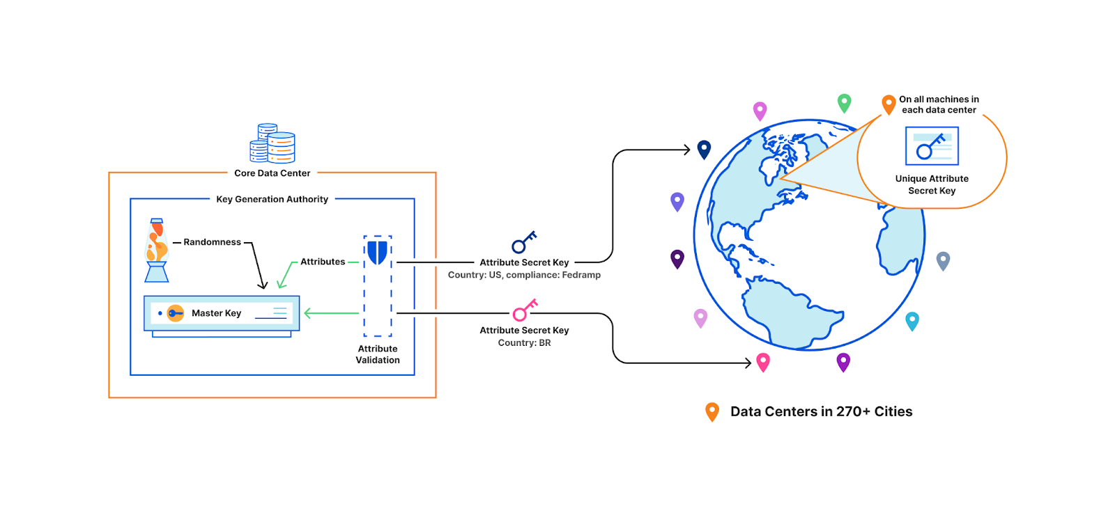
One of the principal challenges we faced with Geo Key Manager v1 (GeoV1) was the inflexibility of our access control policies. Customers required richer data localization, often spurred by regulatory concerns. Internally, events such as the conflict in Ukraine reinforced the need to be able to quickly restrict access to sensitive key material. Geo Key Manager v1’s underlying cryptography was a combination of identity-based broadcast encryption and identity-based revocation that simulated a subset of the functionality offered by Attribute-Based Encryption (ABE). Replacing this with an established ABE scheme addressed the inflexibility of our access control policies and provided a more secure foundation for our system.
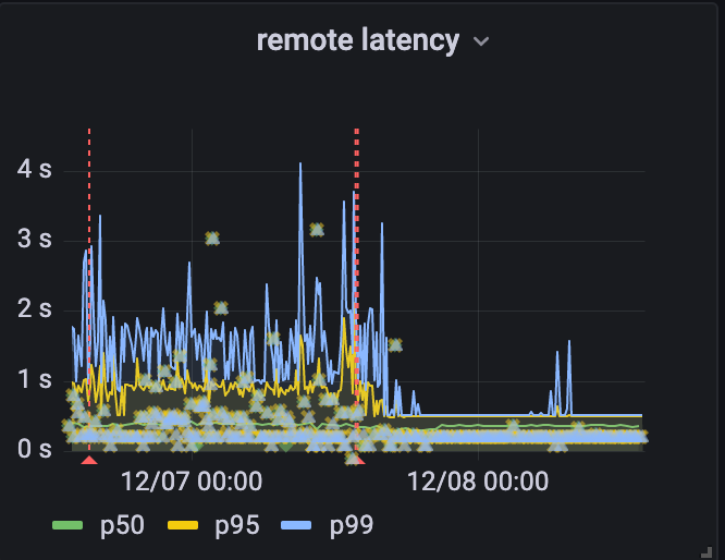
Unlike our previous scheme, which limited future flexibility by freezing the set of participating data centers and policies at the outset, using ABE made the system easily adaptable for future needs. It allowed us to take advantage of performance gains from additional data centers added after instantiation and drastically simplified the process for handling changes to attributes and policies. Furthermore, GeoV1 struggled with some perplexing performance issues that contributed to high tail latency and a painfully manual key rotation process. GeoV2 is our answer to these challenges and limitations of GeoV1.
While this blog focuses on our solution for geographical key management, the lessons here can also be applied to other access control needs. Access control solutions are traditionally implemented using a highly-available central authority to police access to resources. As we will see, ABE allows us to avoid this single point of failure. As there are no large scale ABE-based access control systems we are aware of, we hope our discussion can help engineers consider using ABE as an alternative to access control with minimal reliance on a centralized authority. To facilitate this, we’ve included our implementation of ABE in CIRCL, our open source cryptographic library.
Unsatisfactory attempts at a solution
Before coming back to GeoV2, let’s take a little detour and examine the problem we’re trying to solve.
Consider this example: a large European bank wants to store their TLS private keys only within the EU. This bank is a customer of Cloudflare, which means we perform TLS handshakes on their behalf. The reason we need to terminate TLS for them is so that we can provide the best protection against DDoS attacks, improve performance by caching, support web application firewalls, etc.
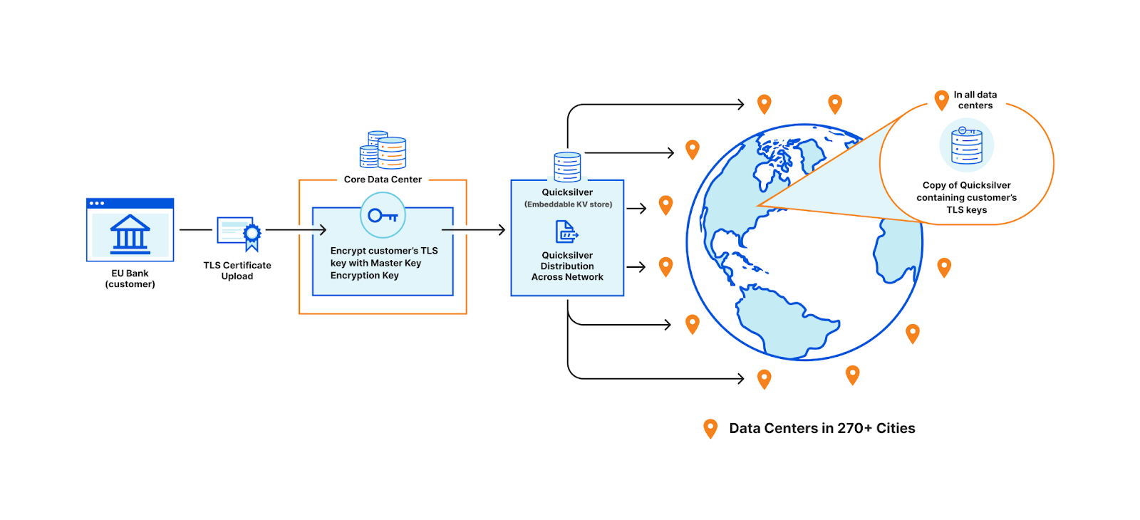
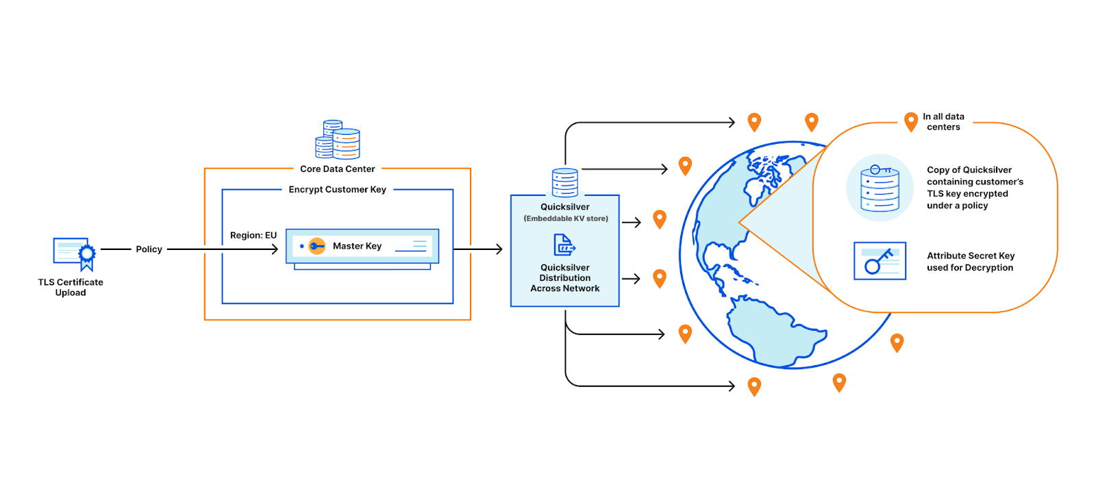
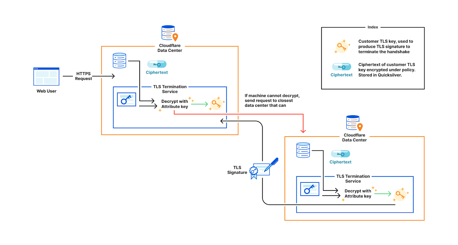
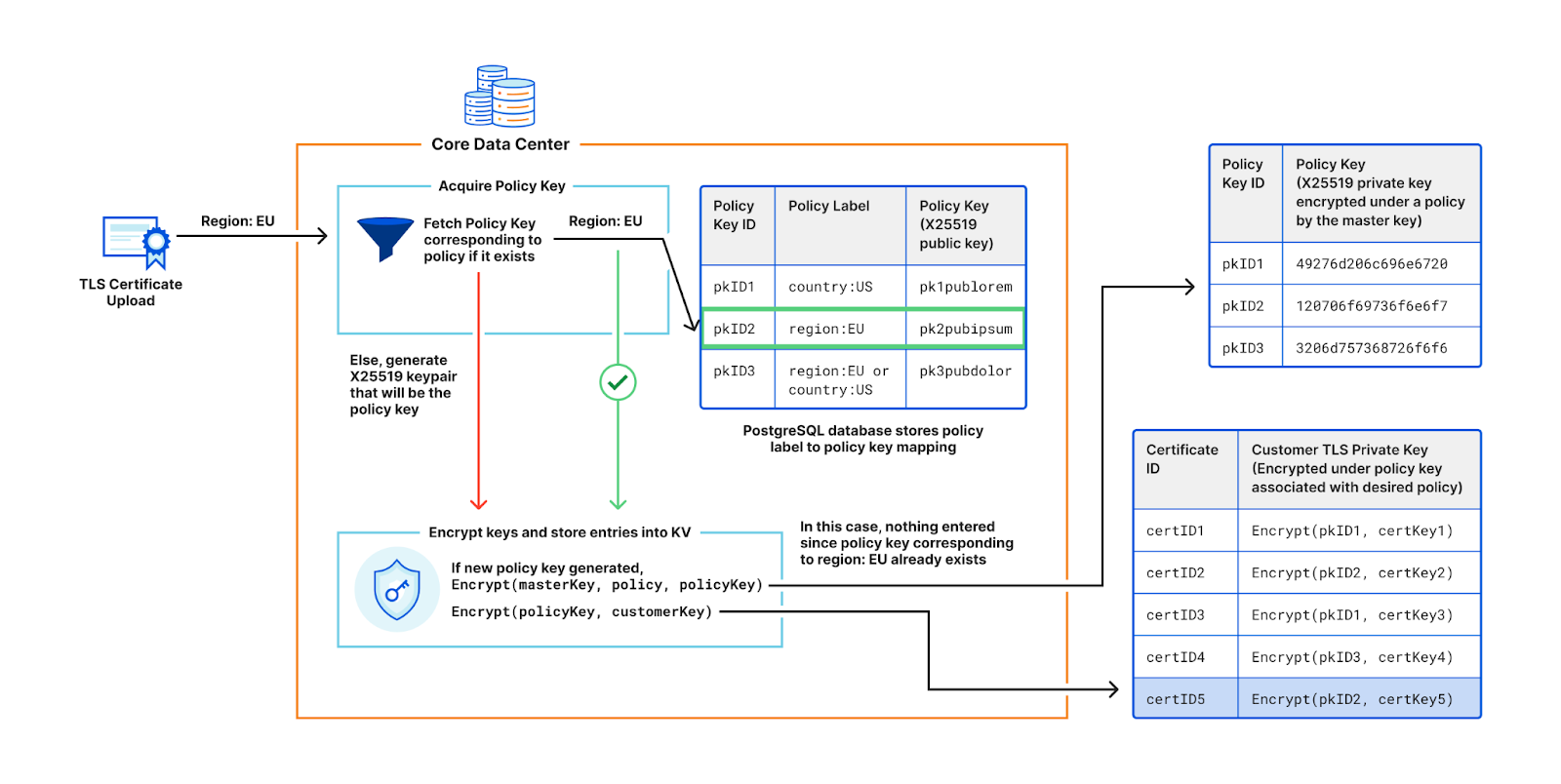
In order to terminate TLS, we need to have access to their TLS private keys1. The control plane, which handles API traffic, encrypts the customer’s uploaded private key with a master public key shared amongst all machines globally. It then puts the key into a globally distributed KV store, Quicksilver. This means every machine in every data center around the world has a local copy of this customer’s TLS private key. Consequently, every machine in each data center has a copy of every customer’s private key.
Customer uploading their TLS certificate and private key to be stored in all data centers
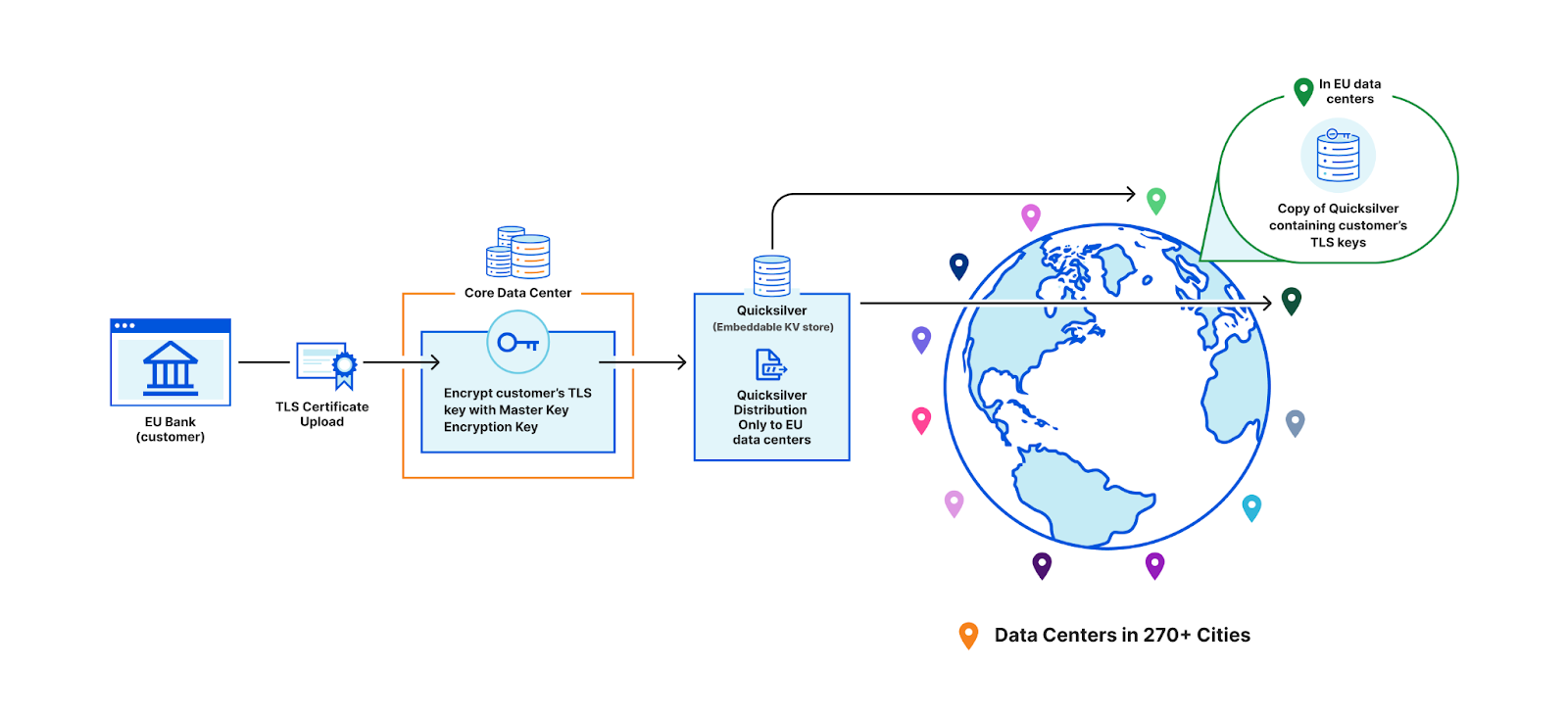
This bank however, wants its key to be stored only in EU data centers. In order to allow this to happen, we have three options.
The first option is to ensure that only EU data centers can receive this key and terminate the handshake. All other machines proxy TLS requests to an EU server for processing. This would require giving each machine only a subset of the entire keyset stored in Quicksilver, which challenges core design decisions Cloudflare has made over the years that assume the entire dataset is replicated on every machine.
Restricting customer keys to EU data centers
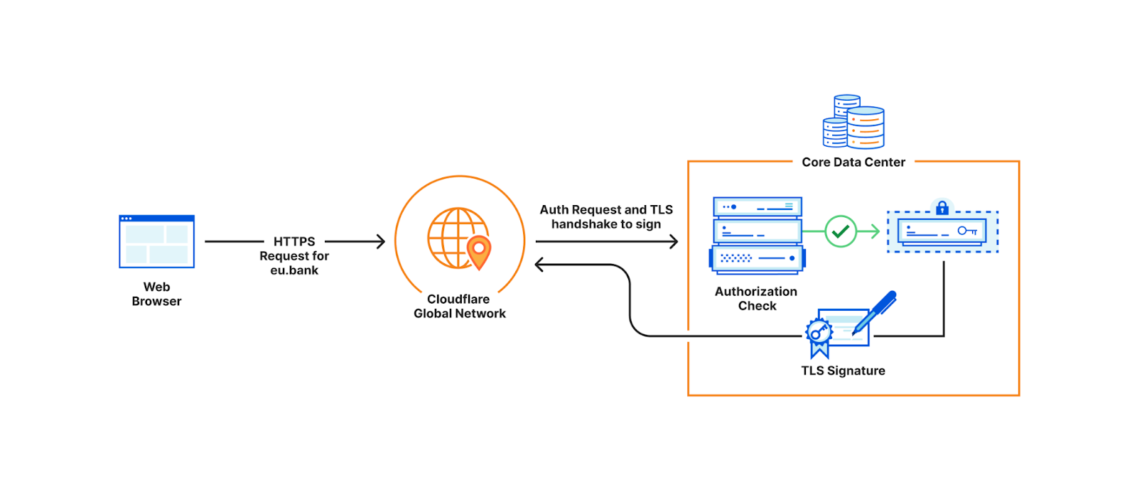
Another option is to store the keys in the core data center instead of Quicksilver. This would allow us to enforce the proper access control policy every time, ensuring that only certain machines can access certain keys. However, this would defeat the purpose of having a global network in the first place: to reduce latency and avoid a single point of failure at the core.
Storing keys in core data center where complicated business logic runs to enforce policies
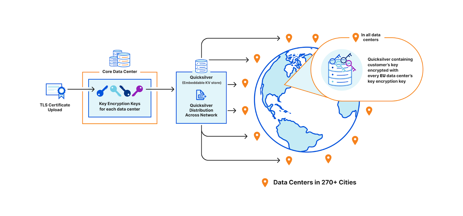
A third option is to use public key cryptography. Instead of having a master key pair, every data center is issued its own key pair. The core encrypts the customer’s private key with the keys of every data center allowed to use it. Only machines in the EU will be able to access the key in this example. Let’s assume there are 500 data centers, with 50 machines each. Of these 500 data centers, let’s say 200 are in the EU. Where 100 keys of 1kB consumed a total of 100 x 500 x 50 x 1 kB (globally), now they will consume 200 times that, and in the worst case, up to 500 times. This increases the space it takes to store the keys on each machine by a whole new factor – before, the storage space was purely a function of how many customer keys are registered; now, the storage space is still a function of the number of customer keys, but also multiplied by the number of data centers.
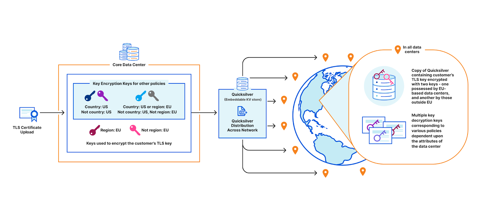
Assigning unique keys to each data center and wrapping customer key with EU data center keys
Unfortunately, all three of these options are undesirable in their own ways. They would either require changing fundamental assumptions we made about the architecture of Cloudflare, abandoning the advantages of using a highly distributed network, or quadratically increasing the storage this feature uses.
A deeper look at the third option reveals – why not create two key pairs instead of a unique one for each data center? One pair would be common among all EU data centers, and one for all non-EU data centers. This way, the core only needs to encrypt the customer’s key twice instead of for each EU data center. This is a good solution for the EU bank, but it doesn’t scale once we start adding additional policies. Consider the example: a data center in New York City could have a key for the policy “country: US”, another one for “country: US or region: EU”, another one for “not country: RU”, and so on… You can already see this getting rather unwieldy. And every time a new data center is provisioned, all policies must be re-evaluated and the appropriate keys assigned.
A key for each policy and its negation
Geo Key Manager v1: identity-based encryption and broadcast encryption
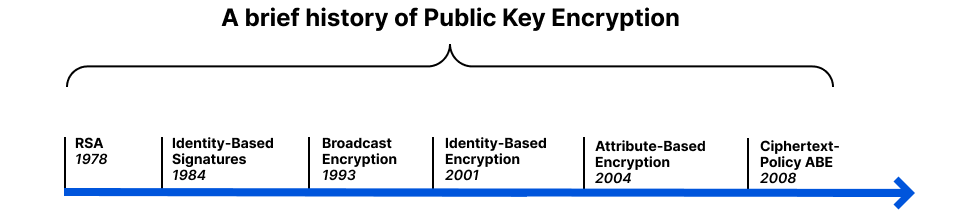
The invention of RSA in 1978 kicked off the era of modern public key cryptography, but anyone who has used GPG or is involved with certificate authorities can attest to the difficulty of managing public key infrastructure that connects keys to user identities. In 1984, Shamir asked if it was possible to create a public-key encryption system where the public key could be any string. His motivation for this question was to simplify email management. Instead of encrypting an email to Bob using Bob’s public key, Alice could encrypt it to Bob’s identity [email protected]. Finally, in 2001, Boneh and Franklin figured out how to make it work.
Broadcast encryption was first proposed in 1993 by Fiat and Naor. It lets you send the same encrypted message to everyone, but only people with the right key can decrypt it. Looking back to our third option, instead of wrapping the customer’s key with the key of every EU data center, we could use broadcast encryption to create a singular encryption of the customer’s key that only EU-based data centers could decrypt. This would solve the storage problem.
Geo Key Manager v1 used a combination of identity-based broadcast encryption and identity-based revocation to implement access control. Briefly, a set of identities is designated for each region and each data center location. Then, each machine is issued an identity-based private key for its region and location. With this in place, access to the customer’s key can be controlled using three sets: the set of regions to encrypt to, the set of locations inside the region to exclude, and the set of locations outside the region to include. For example, the customer’s key could be encrypted so that it is available in all regions except for a few specific locations, and also available in a few locations outside those regions. This blog post has all the nitty-gritty details of this approach.
Unfortunately this scheme was insufficiently responsive to customer needs; the parameters used during initial cryptographic setup, such as the list of regions, data centers, and their attributes, were baked into the system and could not be easily changed. Tough luck excluding the UK from the EU region post Brexit, or supporting a new region based on a recent compliance standard that customers need. Using a predetermined static list of locations also made it difficult to quickly revoke machine access. Additionally, decryption keys could not be assigned to new data centers provisioned after setup, preventing them from speeding up requests. These limitations provided the impetus for integrating Attribute-Based Encryption (ABE) into Geo Key Manager.
Attribute-Based Encryption
In 2004, Amit Sahai and Brent Waters proposed a new cryptosystem based on access policies, known as attribute-based encryption (ABE). Essentially, a message is encrypted under an access policy rather than an identity. Users are issued a private key based on their attributes, and they can only decrypt the message if their attributes satisfy the policy. This allows for more flexible and fine-grained access control than traditional methods of encryption.
Brief timeline of Public Key Encryption
The policy can be attached either to the key or to the ciphertext, leading to two variants of ABE: key-policy attribute-based encryption (KP-ABE) and ciphertext-policy attribute-based encryption (CP-ABE). There exist trade-offs between them, but they are functionally equivalent as they are duals of each other. Let’s focus on CP-ABE it aligns more closely with real-world access control. Imagine a hospital where a doctor has the attributes “role: doctor” and “region: US”, while a nurse has the attributes “role: nurse” and “region: EU”. A document encrypted under the policy “role: doctor or region: EU” can be decrypted by both the doctor and nurse. In other words, ABE is like a magical lock that only opens for people who have the right attributes.
Policy
Semantics
country: US or region: EU
Decryption is possible either in the US or in the European Union
not (country: RU or country: US)
Decryption is not possible in Russia and US
country: US and security: high
Decryption is possible only in data centers within the US that have a high level of security (for some security definition established previously)
There are many different ABE schemes out there, with varying properties. The scheme we choose must satisfy a few requirements:
Negation We want to be able to support boolean formulas consisting of AND, OR and NOT, aka non-monotonic boolean formulas. While practically every scheme handles AND and OR, NOT is rarer to find. Negation makes blocklisting certain countries or machines easier.
Repeated Attributes Consider the policy “organization: executive or (organization: weapons and clearance: top-secret)”. The attribute “organization” has been repeated twice in the policy. Schemes with support for repetition add significant expressibility and flexibility when composing policies.
Security against Chosen Ciphertext Attacks Most schemes are presented in a form that is only secure if the attacker doesn’t choose the messages to decrypt (CPA). There are standard ways to convert such a scheme into one that is secure even if the attacker manipulates ciphertexts (CCA), but it isn’t automatic. We apply the well-known Boneh-Katz transform to our chosen scheme to make it secure against this class of attacks. We will present a proof of security for the end to end scheme in our forthcoming paper.
Negation in particular deserves further comment. For an attribute to be satisfied when negated, the name must stay the same, but the value must differ. It’s like the data center is saying, “I have a country, but it’s definitely not Japan”, instead of “I don’t have a country”. This might seem counterintuitive, but it enables decryption without needing to examine every attribute value. It also makes it safe to roll out attributes incrementally. Based on these criteria, we ended up choosing the scheme by Tomida et al (2021).
Implementing a complex cryptographic scheme such as this can be quite challenging. The discrete log assumption that underlies traditional public key cryptography is not sufficient to meet the security requirements of ABE. ABE schemes must secure both ciphertexts and the attribute-based secret keys, whereas traditional public key cryptography only imposes security constraints on the ciphertexts, while the secret key is merely an integer. To achieve this, most ABE schemes are constructed using a mathematical operation known as bilinear pairings.
The speed at which we can perform pairing operations determines the baseline performance of our implementation. Their efficiency is particularly desirable during decryption, where they are used to combine the attribute-based secret key with the ciphertext in order to recover the plaintext. To this end, we rely on our highly optimized pairing implementations in our open source library of cryptographic suites, CIRCL, which we discuss at length in a previous blog. Additionally, the various keys, attributes and the ciphertext that embeds the access structure are expressed as matrices and vectors. We wrote linear algebra routines to handle matrix operations such as multiplication, transpose, inverse that are necessary to manipulate the structures as needed. We also added serialization, extensive testing and benchmarking. Finally, we implemented our conversion to a CCA2 secure scheme.
In addition to the core cryptography, we had to decide how to express and represent policies. Ultimately we decided on using strings for our API. While perhaps less convenient for programs than structures would be, users of our scheme would have to implement a parser anyway. Having us do it for them seemed like a way to have a more stable interface. This means the frontend of our policy language was composed of boolean expressions as strings, such as “country: JP or (not region: EU)”, while the backend is a monotonic boolean circuit consisting of wires and gates. Monotonic boolean circuits only include AND and OR gates. In order to handle NOT gates, we assigned positive or negative values to the wires. Every NOT gate can be placed directly on a wire because of De Morgan’s Law, which allows the conversion of a formula like “not (X and Y)” into “not X or not Y”, and similarly for disjunction.
The following is a demonstration of the API. The central authority runs Setup to generate the master public key and master secret key. The master public key can be used by anyone to encrypt a message over an access policy. The master secret key, held by the central authority, is used to generate secret keys for users based on their attributes. Attributes themselves can be supplied out-of-band. In our case, we rely on the machine provisioning database to provide and validate attributes. These attribute-based secret keys are securely distributed to users, such as over TLS, and are used to decrypt ciphertexts. The API also includes helper functions to check decryption capabilities and extract policies from ciphertexts for improved usability.
We now come back to our original example. This time, the central authority holds the master secret key. Each machine in every data center presents its set of attributes to the central authority, which, after some validation, generates a unique attribute-based secret key for that particular machine. Key issuance happens when a machine is first brought up, if keys must be rotated, or if an attribute has changed, but never in the critical path of a TLS handshake. This solution is also collusion resistant, which means two machines without the appropriate attributes cannot combine their keys to decrypt a secret that they individually could not decrypt. For example, a machine with the attribute “country: US” and another with “security: high”. These machines cannot collude together to decrypt a resource with the policy “country: US and security: high”.
Crucially, this solution can seamlessly scale and respond to changes to machines. If a new machine is added, the central authority can simply issue it a secret key since the participants of the scheme don’t have to be predetermined at setup, unlike our previous identity-broadcast scheme.
Key Distribution
When a customer uploads their TLS certificate, they can specify a policy, and the central authority will encrypt their private key with the master public key under the specified policy. The encrypted customer key then gets written to Quicksilver, to be distributed to all data centers. In practice, there is a layer of indirection here that we will discuss in a later section.
Encryption using Master Public Key
When a user visits the customer’s website, the TLS termination service at the data center that first receives the request, fetches the customer’s encrypted private key from Quicksilver. If the service’s attributes do not satisfy the policy, decryption fails and the request is proxied to the closest data center that satisfies the policy. Whichever data center can successfully decrypt the key performs the signature to complete the TLS handshake.
Decryption using Attribute-based Secret Key (Simplified)
The following table summarizes the pros and cons of the various solutions we discussed:
Solution
Flexible policies
Fault Tolerant
Efficient Space
Low Latency
Collusion-resistant
Changes to machines
Different copies of Quicksilver in data centers
✅
✅
✅
✅
✅
Complicated Business Logic in Core
✅
✅
✅
✅
Encrypt customer keys with each data center’s unique keypair
✅
✅
✅
✅
Encrypt customer keys with a policy-based keypair, where each data center has multiple policy-based keypairs
We characterize our scheme’s performance on measures inspired by ECRYPT. We set the attribute size to 50, which is significantly higher than necessary for most applications, but serves as a worst case scenario for benchmarking purposes. We conduct our measurements on a laptop with Intel Core i7-10610U CPU @ 1.80GHz and compare the results against RSA with 2048-bit security, X25519 and our previous scheme.
Scheme
Secret key(bytes)
Public key(bytes)
Overhead of encrypting 23 bytes (ciphertext length – message length)
Overhead of encrypting 10k bytes (ciphertext length – message length)
RSA-2048
1190 (PKCS#1)
256
233
3568
X25519
32
32
48
48
GeoV1 scheme
4838
4742
169
169
GeoV2 ABE scheme
33416
3282
19419
19419
Different attribute based encryption schemes optimize for different performance profiles. Some may have fast key generation, while others may prioritize fast decryption. In our case, we only care about fast decryption because it is the only part of the process that lies in the critical path of a request. Everything else happens out-of-band where the extra overhead is acceptable.
Scheme
Generating keypair
Encrypting 23 bytes
Decrypting 23 bytes
RSA-2048
117 ms
0.043 ms
1.26 ms
X25519
0.045 ms
0.093 ms
0.046 ms
GeoV1 scheme
75 ms
10.7 ms
13.9 ms
GeoV2 ABE scheme
1796 ms
704 ms
62.4 ms
A Brief Note on Attribute-Based Access Control (ABAC)
ABAC is an extension of the more familiar Role-Based Access Control (RBAC). To understand why ABAC is relevant, let’s briefly discuss its origins. In 1970, the United States Department of Defense introduced Discretionary Access Control (DAC). DAC is how Unix file systems are implemented. But DAC isn’t enough if you want to restrict resharing, because the owner of the resource can grant other users permission to access it in ways that the central administrator does not agree with. To address this, the Department of Defense introduced Mandatory Access Control (MAC). DRM is a good example of MAC. Even though you have the file, you don’t have a right to share it to others.
RBAC is an implementation of certain aspects of MAC. ABAC is an extension of RBAC that was defined by NIST in 2017 to address the increasing characteristics of users that are not restricted to their roles, such as time of day, user agent, and so on.
However, RBAC/ABAC is simply a specification. While they are traditionally implemented using a central authority to police access to some resource, it doesn’t have to be so. Attribute-based encryption is an excellent mechanism to implement ABAC in distributed systems.
Key rotation
While it may be tempting to attribute all failures to DNS, changing keys is another strong contender in this race. Suffering through the rather manual and error-prone key rotation process of Geo Key Manager v1 taught us to make robust and simple key rotation without impact on availability, an explicit design goal for Geo Key Manager v2.
To facilitate key rotation and improve performance, we introduce a layer of indirection to the customer key wrapping (encryption) process. When a customer uploads their TLS private key, instead of encrypting with the Master Public Key, we generate a X25519 keypair, called the policy key. The central authority then adds the public part of this newly minted policy keypair and its associated policy label to a database. It then encrypts the private half of the policy keypair with the Master Public Key, over the associated access policy. The customer’s private key is encrypted with the public policy key, and saved into Quicksilver.
When a user accesses the customer’s website, the TLS termination service at the data center that receives the request fetches the encrypted policy key associated with the customer’s access policy. If the machine’s attributes don’t satisfy the policy, decryption fails and the request is forwarded to the closest satisfying data center. If decryption succeeds, the policy key is used to decrypt the customer’s private key and complete the handshake.
Key
Purpose
CA in core
Core
Network
Master Public Key
Encrypts private policy keys over an access policy
Generate
Read
Master Secret Key
Generates secret keys for machines based on their attributes
Generate,Read
Machine Secret Key / Attribute-Based Secret Key
Decrypts private policy keys stored in global KV store, Quicksilver
Generate
Read
Customer TLS Private Key
Performs digital signature necessary to complete TLS handshake to the customer’s website
Read (transiently on upload)
Read
Public Policy Key
Encrypts customers’ TLS private keys
Generate, Read
Private Policy Key
Decrypts customer’s TLS private keys
Read (transiently during key rotation)
Generate
Read
However, policy keys are not generated for every customer’s certificate upload. As shown in the figure below, if a customer requests a policy that already exists in the system and thus has an associated policy key, the policy key will get re-used. Since most customers use the same few policies, such as restricting to one country, or restricting to the EU, the number of policy keys is orders of magnitude smaller compared to the number of customer keys.
Policy Keys
This sharing of policy keys is tremendously useful for key rotation. When master keys are rotated (and consequently the machine secret keys), only the handful of policy keys used to control access to the customers’ keys need to be re-encrypted, rather than every customer’s key encryption. This reduces compute and bandwidth requirements. Additionally, caching policy keys at the TLS termination service improves performance by reducing the need for frequent decryptions in the critical path.
This is similar to hybrid encryption, where public key cryptography is used to establish a shared symmetric key, which then gets used to encrypt data. The difference here is that the policy keys are not symmetric, but rather X25519 keypairs, which is an asymmetric scheme based on elliptic curves. While not as fast as symmetric schemes like AES, traditional elliptic curve cryptography is significantly faster than attribute-based encryption. The advantage here is that the central service doesn’t need access to secret key material to encrypt customer keys.
The other component of robust key rotation involves maintaining multiple key versions.The latest key generation is used for encryption, but the latest and previous versions can be used for decryption. We use a system of states to manage key transitions and safe deletion of older keys. We also have extensive monitoring in place to alert us if any machines are not using the appropriate key generations.
The Tail At Scale
Geo Key Manager suffered from high tail latency, which occasionally impacted availability. Jeff Dean’s paper, The Tail at Scale, is an enlightening read on how even elevated p99 latency at Cloudflare scale can be damaging. Despite revamping the server and client components of our service, the p99 latency didn’t budge. These revamps, such as switching from worker pools to one goroutine per request, did simplify the service, as they removed thousands of lines of code. Distributed tracing was able to pin down the delays: they took place between the client sending a request and the server receiving it. But we could not dig in further. We even wrote a blog last year describing our debugging endeavors, but without a concrete solution.
Finally, we realized that there is a level of indirection between the client and the server. Our data centers around the world are very different sizes. To avoid swamping smaller data centers with connections, larger data centers would task individual, intermediary machines with proxying requests to other data centers using the Go net/rpc library.
Once we included the forwarding function on the intermediary server in the trace, the problem became clear. There was a long delay between issuing the request and processing it. Yet the code was merely a call to a built-in library function. Why was it delaying the request?
Ultimately we found that there was a lock held while the request was serialized. The net/rpc package does not support streams, but our packet-oriented custom application protocol, which we wrote before the advent of gRPC, does support streaming. To bridge this gap, we executed a request and waited for the response in the serialization function. While an expedient way to get the code written, it created a performance bottleneck as only one request could be forwarded at a time.
Our solution was to use channels for coordination, letting multiple requests execute while we waited for the responses to arrive. When we rolled it out we saw dramatic decreases in tail latency.
The results of fixing RPC failures in remote colo in Australia
Unfortunately we cannot make the speed of light any faster (yet). Customers who want their keys kept only in the US while their website users are in the land down under will have to endure some delays as we make the trans-pacific voyage. But thanks to session tickets, those delays only affect new connections.
Uptime was also significantly improved. Data centers provisioned after cryptographic initiation could now participate in the system, which also implies that data centers that did not satisfy a certain policy had a broader range of satisfying neighbors to which they could forward the signing request to. This increased redundancy in the system, and particularly benefited data centers in regions without the best internet connectivity. The graph below represents successful probes spanning every machine globally over a two-day period. For GeoV1, we see websites with policies for US and EU regions falling to under 98% at one point, while for GeoV2, uptime rarely drops below 4 9s of availability.
Uptime by Key Profile across US and EU for GeoV1 and GeoV2, and IN for GeoV2
Conclusion
Congratulations dear reader for making it this far. Just like you, applied cryptography has come a long way, but only limited slivers manage to penetrate the barrier between research and real-world adoption. Bridging this gap can help enable novel capabilities for protecting sensitive data. Attribute-based encryption itself has become much more efficient and featureful over the past few years. We hope that this post encourages you to consider ABE for your own access control needs, particularly if you deal with distributed systems and don’t want to depend on a highly available central authority. We have open-sourced our implementation of CP-ABE in CIRCL, and plan on publishing a paper with additional details.
We look forward to the numerous product improvements to Geo Key Manager made possible by this new cryptographic foundation. We plan to use this ABE-based mechanism for storing not just private keys, but also other types of data. We are working on making it more user-friendly and generalizable for internal services to use.
Acknowledgements
We’d like to thank Watson Ladd for his contributions to this project during his tenure at Cloudflare.
…… 1While true for most customers, we do offer Keyless SSL that allows customers who can run their own keyservers, the ability to store their private keys on-prem
Today we mark the International Holocaust Remembrance Day. We commemorate the victims that were robbed of their possessions, stripped of their rights, deported, starved, dehumanized and murdered by the Nazis and their accomplices. During the Holocaust and in the events that led to it, the Nazis exterminated one third of the European Jewish population. Six million Jews, along with countless other members of minority and disability groups, were murdered because the Nazis believed they were inferior.
Seventy eight years later, after the liberation of the infamous Auschwitz death camp, antisemitism still burns with hatred. According to a study performed by the Campaign Against Antisemitism organization on data provided by the UK Home Office, Jews are 500% more likely to be targeted by hate crime than any other faith group per capita.
From Cloudflare’s vantage point we can point to distressing findings as well. In 2021, cyberattacks on Holocaust educational websites doubled year over year. In 2021, one out of every 100 HTTP requests sent to Holocaust educational websites behind Cloudflare was part of an attack. In 2022, the share of those cyber attacks grew again by 49% YoY. Cyberattacks represented 1.6% of all traffic to Holocaust educational websites (almost 1 out of every 50 HTTP requests), as can be seen in the chart below in 2022.
We’re representing cyberattacks as a percentage to normalize natural growth of traffic to websites, mitigation methods and other potential data biases. But even if we look at the raw numbers, between 2021 and 2022, the absolute cyberattack traffic (in HTTP requests) that targeted Holocaust education websites behind Cloudflare grew by 640% in contrast to the total growth of 397% in the number of all requests (attack and non-attack HTTP requests).
Share of cyberattack targeting Holocaust education websites
(Please note that the graph starts in 95% in order to provide better visibility into the share of attacks)
The threat that Holocaust educational websites face is one that many other non-profit organizations face. In fact, in our most recent DDoS Trends report, non-profit organizations were the sixth most targeted industry. Ten percent of all traffic to non-profit websites behind Cloudflare was DDoS attack traffic.
Top industries targeted by HTTP DDoS attacks in 2022 Q4
However, nonprofits such as Holocaust educational organizations might not always have the resources to fend off attacks. For this reason, we provide free protection to at-risk groups across the world. We do this through Project Galileo. It helps keep vulnerable websites online. It provides free cyber security services for groups working in the arts, human rights, civil society, journalism, or democracy. As detailed in our recent Impact Report, in 2022, through Project Galileo, we protected vulnerable websites from an average of 59M cyber threats every day.
If you’re representing a vulnerable public interest group and want to protect your website with Project Galileo, please follow the steps and apply here. While you wait to hear back, you can also get started with our Free plan.
At Cloudflare, we remember and never forget.
Here at Cloudflare, some of us are descendants of Holocaust survivors. My grandparents escaped Nazi-occupied Poland after the German invasion. Sadly, my grandparents — as other elderly survivors, have already passed. I grew up hearing about their stories of bravery — and of deep torment. It’s not always easy to hear these stories, but we must — especially in times like these when war in Europe has been ongoing for almost a year now. We have the responsibility to ensure the world remembers and never forgets the atrocities of the Holocaust and what antisemitism, racism and hatred in general can lead to.
To this extent, a few months ago, here at the Cloudflare London office, we had the honor of hosting Janine Webber, recipient of the British Empire Medal (BEM) in an event hosted by Judeoflare, Cloudflare’s Jewish employee resource group. The event was made possible due to our partnership with the Holocaust Education Trust. And so in a fully packed auditorium and an oversubscribed Zoom call, we listen to Janine’s story of survival and bravery first hand. We asked questions and we learned.
We’re privileged to be able to share her story here with all of you via Cloudflare TV.
In this blog post, you will learn how to set up monitoring for your Litter Robot 3. There’s some amazing community scripts already available to connect to the Litter Robot through a selfmade API, which we’ll be using in combination with some Python scripts and Zabbix.
Introduction
Technology is everywhere. On the streets, in our offices and even in our houses. This also means that many people have ‘smart’ lighting, fridges, cameras and a lot more. Personally, I have avoided these home automations for a long time, deeming them time-consuming. But, I think any IT Engineer sometimes feels there is a need to build and automate more and more. Thus, my house has also had a bit of smart home make-over and I’ve started setting up Zabbix at home to monitor everything ‘smart’.
One of the things I cannot live without in our house is our smart litterbox. It keeps the litterbox clean and the smell in the house nice, as well as it provides some very useful insights into my cats ‘potty’ behaviour. One of my cats “Jerry” has some issues with Feline Urinary Tract Disease (FLUTD). This has led Jerry to have some odd litterbox usage, which in his case can be fatal if not treated early on.
So, let’s bring Zabbix into the mix! Even though the Litter Robot has an app where I can see the usage, I want to be able to receive alerts from Zabbix if the Litter Robot usage goes over a certain threshold. Alerting me early on if issues might be arising again. Let’s set things up.
How to
Setting up the script
To make this all possible, we will need to get some information from our Litter Robot or Litter Robots if we have more than one in our account. There’s no official documented API available for the Litter Robot, but there is a way to get information from the device by connecting to the Whisker services. To make things easy for us, we’ll be using a community-made Python library to set up the connection and execute some functions:
https://github.com/natekspencer/pylitterbot
This library contains a number of functions that we can utilize to get information from the Litterbox, but also to make changes to it:
refresh()
start_cleaning()
reset_settings()
set_panel_lockout()
set_night_light()
set_power_status()
set_sleep_mode()
set_wait_time()
set_name()
reset_waste_drawer()
get_activity_history()
get_insight()
Utilizing this library we’ve made some scripts available at the Github page below.
These scripts will have to be executed by Zabbix server’s (or proxy’s) local Zabbix agent, and thus we’ll also have to download the correct UserParameter files.
cd /etc/zabbix/zabbix_agent2.d/
or
cd /etc/zabbix/zabbix_agentd.d/

wget https://raw.githubusercontent.com/OpensourceICTSolutions/zabbix-litterrobot/main/litterrobot_userparams.conf
Then, we have to make sure that the Zabbix agent will be able to use these new parameters by enabling unsafe user parameter option (since there is an @ in the username). Edit /etc/zabbix/zabbix_agent2.conf or /etc/zabbix/zabbix_agentd.conf and add the following:
UnsafeUserParameters=1
Then we restart the agent with the following command:
systemctl restart zabbix-agent
or
systemctl restart zabbix-agent2
Setting up Zabbix
With the scripts in place and the Zabbix agent ready to execute them, we can set up our monitoring in the Zabbix frontend. To do this, we will have to download and import the template. You can find the 6.2 version template here: https://github.com/OpensourceICTSolutions/zabbix-litterrobot/blob/main/zabbix_litterrobot_python_template.yaml
After downloading the template, import it into Zabbix.
Create a new host for your Litter Robot:
Then make sure to add your username and password as macros:
The result
The result is that we can now find all of our important information about the Litter Robot 3 in Zabbix:
Not only that, after we have an idea of how many times per day our cat(s) usually go to the toilet we can start to use the triggers:
There’s a message for when the drawer is full, but also a Warning and High trigger for when there are more than 12 or 15 cycles respectively. This is a default set for my two cats, your cats might have different potty behavior – update your macros accordingly.
As well as create some useful graphs:
Conclusion
Our pets are a big part of our life and sometimes it can be hard to communicate with them. Cats are very likely to hide their feelings, but one of the telling signs something is wrong with them is the number of times they visit the litterbox. Jerry has had a hard time, but our Litter Robot has helped us and our veterinary keep an eye on him to get ahead of his FLUTD. Using Zabbix we can keep Jerry out of surgery as much as possible.
And keep both (Midna on the left, Jerry on the right) of them racing through the house and enjoying all of their 9 lives.
I hope you enjoyed reading this blog post and if you have any questions or need help configuring anything in your Zabbix setup feel free to contact me and the team at Opensource ICT Solutions. We build a ton of cool integrations like this and much more!
To provide the best experiences, we use technologies like cookies to store and/or access device information. Consenting to these technologies will allow us to process data such as browsing behavior or unique IDs on this site. Not consenting or withdrawing consent, may adversely affect certain features and functions.
Functional
Always active
The technical storage or access is strictly necessary for the legitimate purpose of enabling the use of a specific service explicitly requested by the subscriber or user, or for the sole purpose of carrying out the transmission of a communication over an electronic communications network.
Preferences
The technical storage or access is necessary for the legitimate purpose of storing preferences that are not requested by the subscriber or user.
Statistics
The technical storage or access that is used exclusively for statistical purposes.The technical storage or access that is used exclusively for anonymous statistical purposes. Without a subpoena, voluntary compliance on the part of your Internet Service Provider, or additional records from a third party, information stored or retrieved for this purpose alone cannot usually be used to identify you.
Marketing
The technical storage or access is required to create user profiles to send advertising, or to track the user on a website or across several websites for similar marketing purposes.
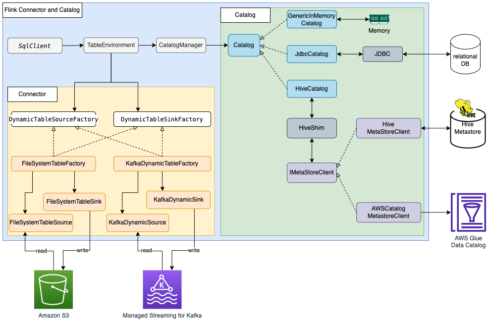
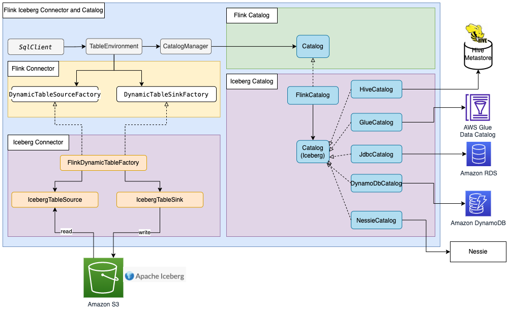

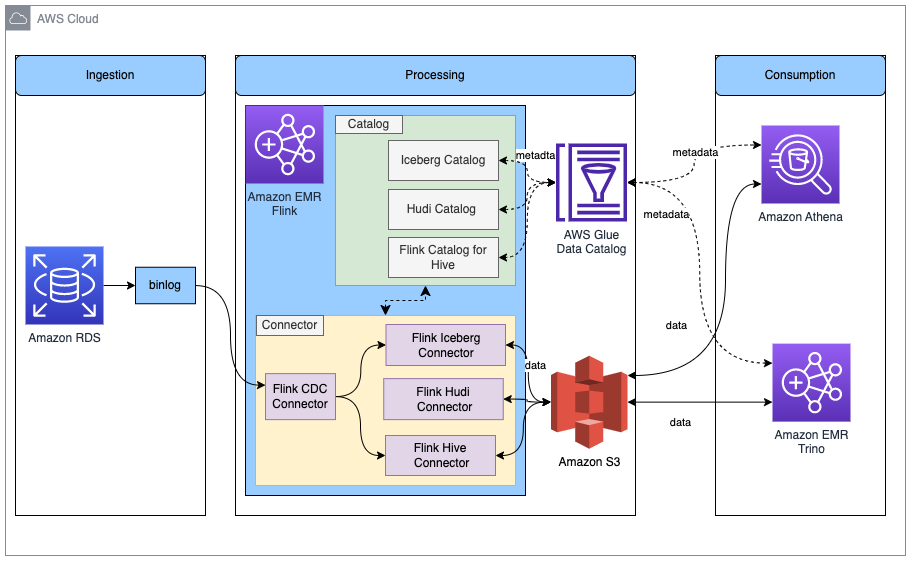
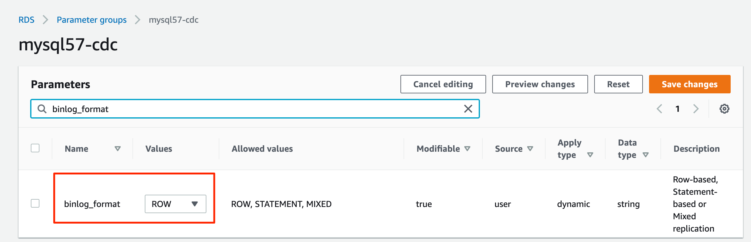
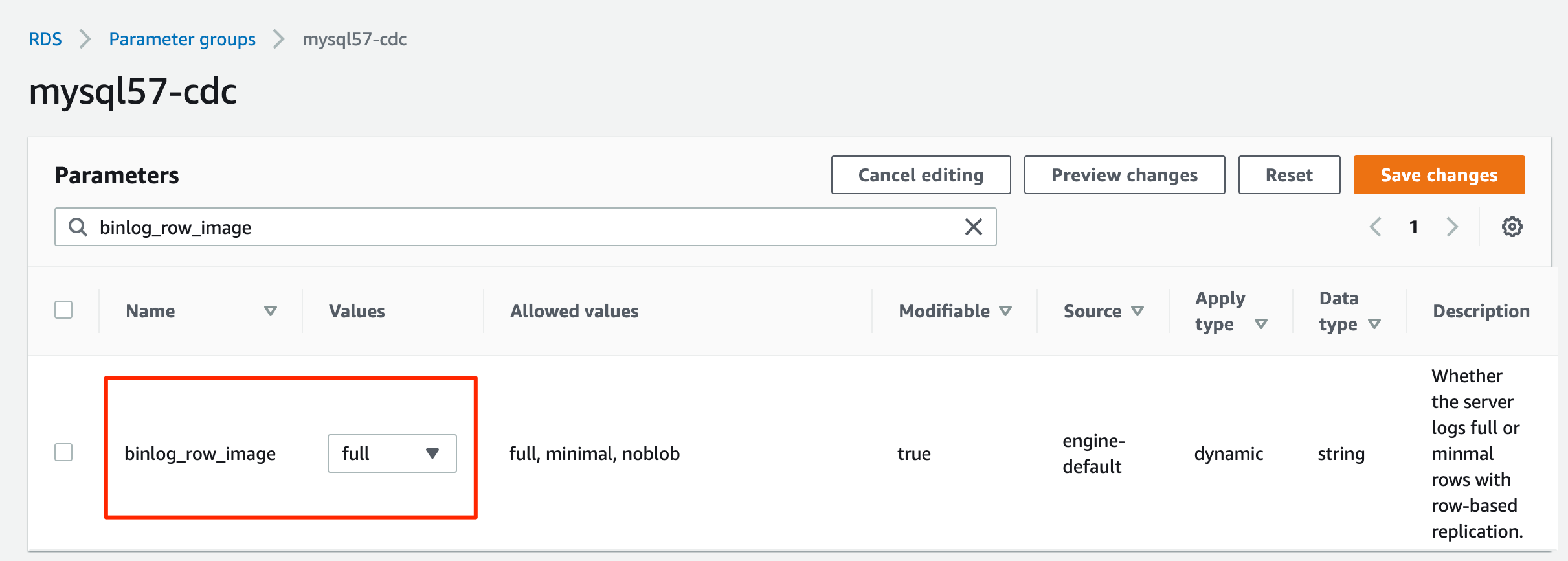


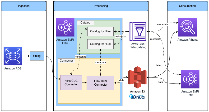
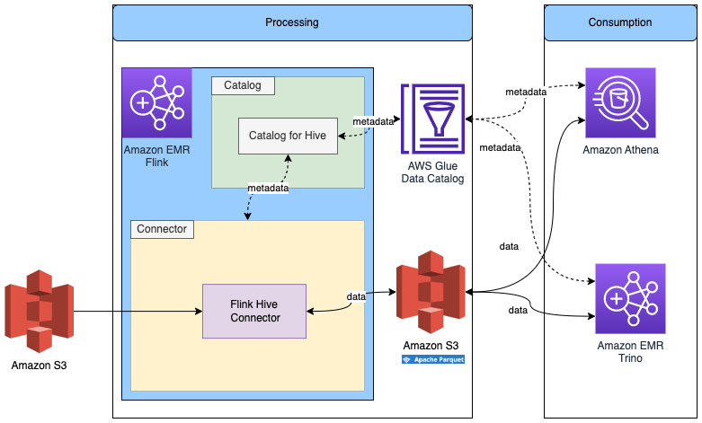


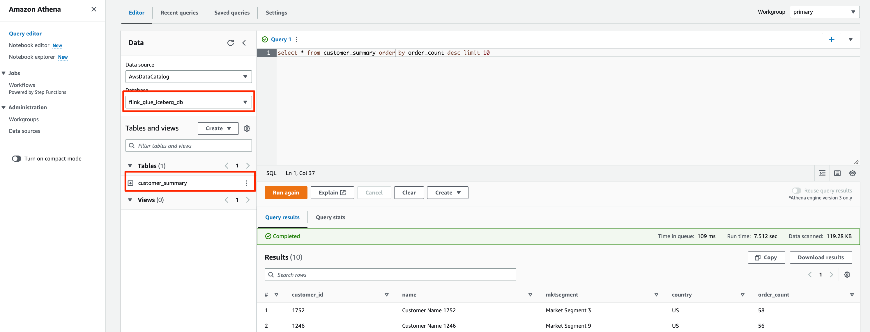


 Mehmet Demir is a Senior Solutions Architect at Amazon Web Services (AWS) based in Toronto, Canada. He helps customers in building well-architected solutions that support business innovation.
 Ankur Taunk is a Senior Specialist Solutions Architect at AWS. He helps customer achieve their desired business outcomes in the Contact Center space leveraging Amazon Connect.
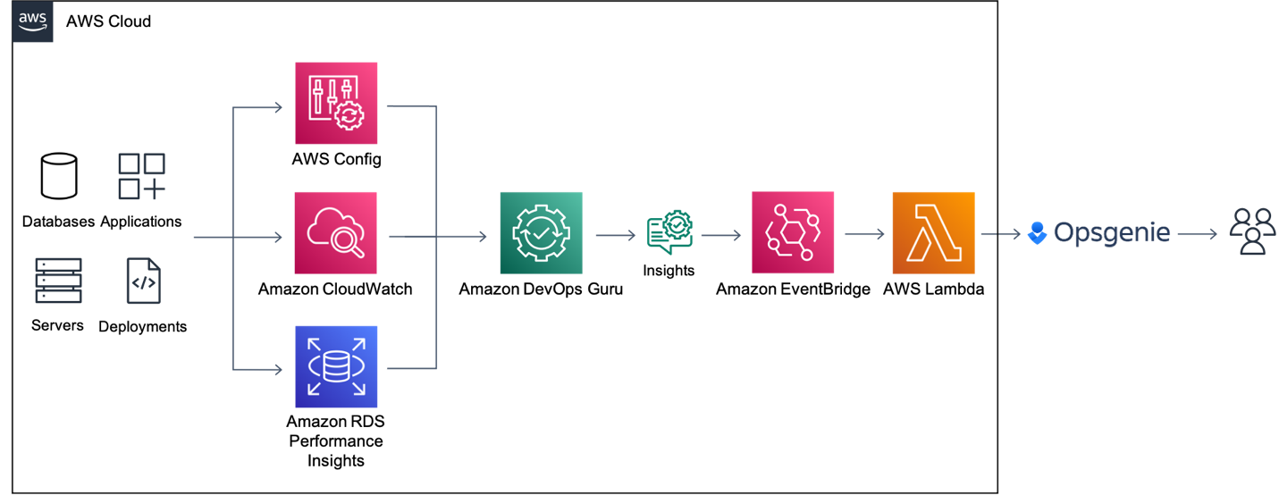
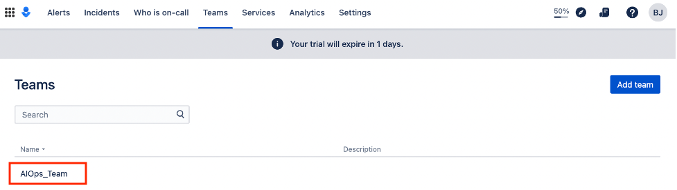
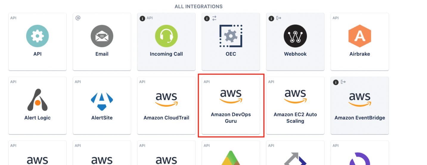

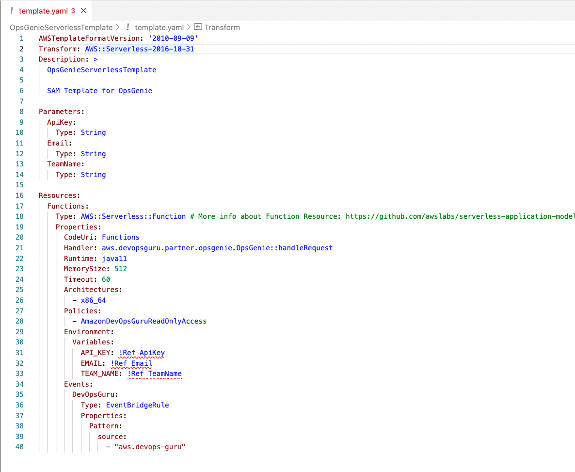
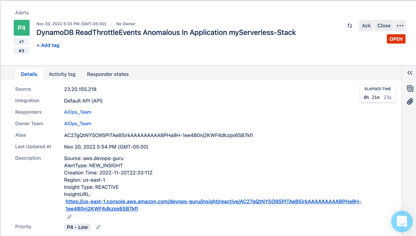
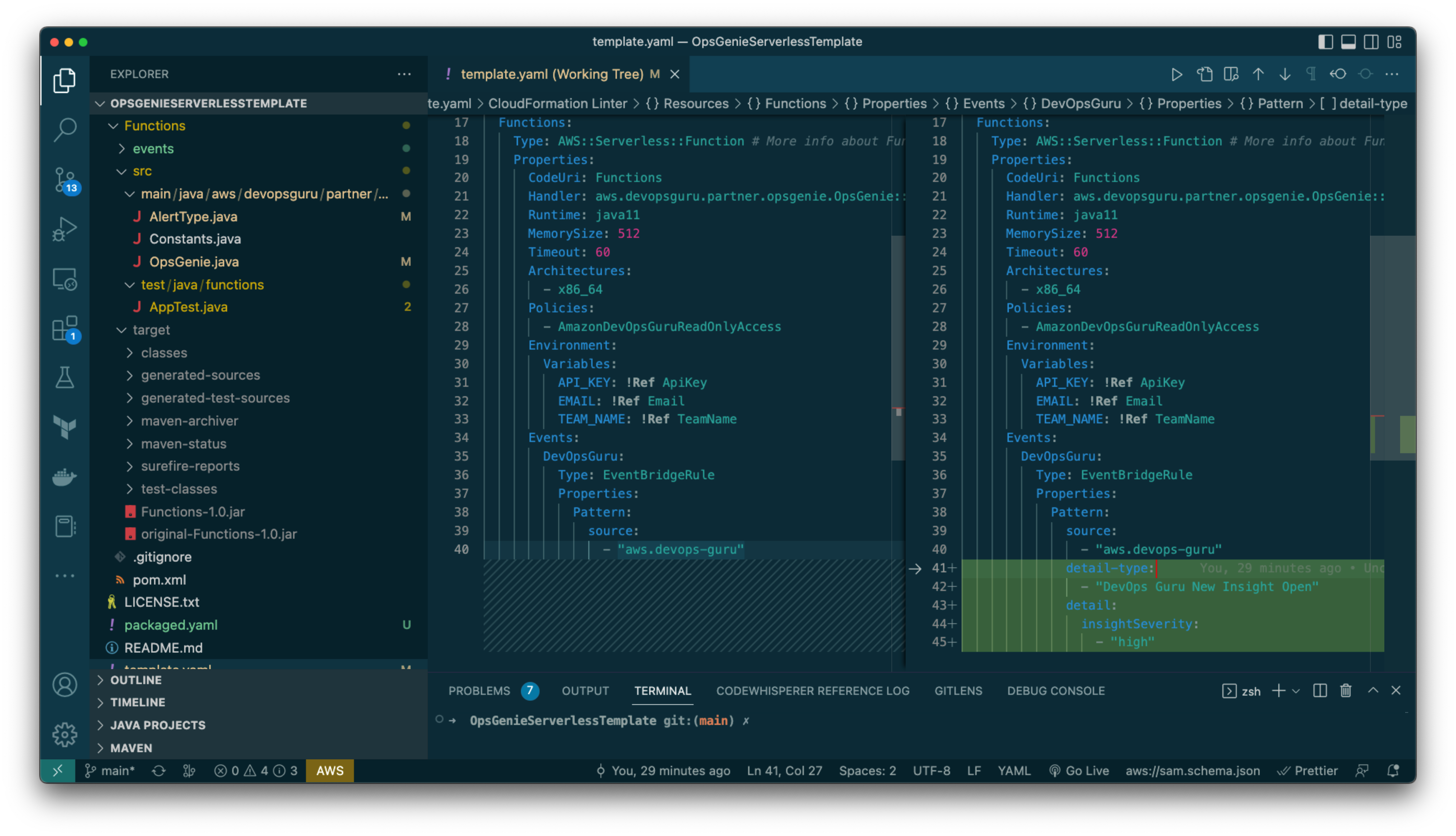
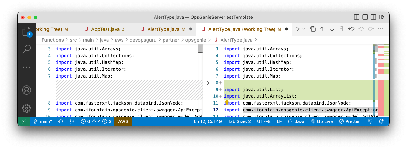
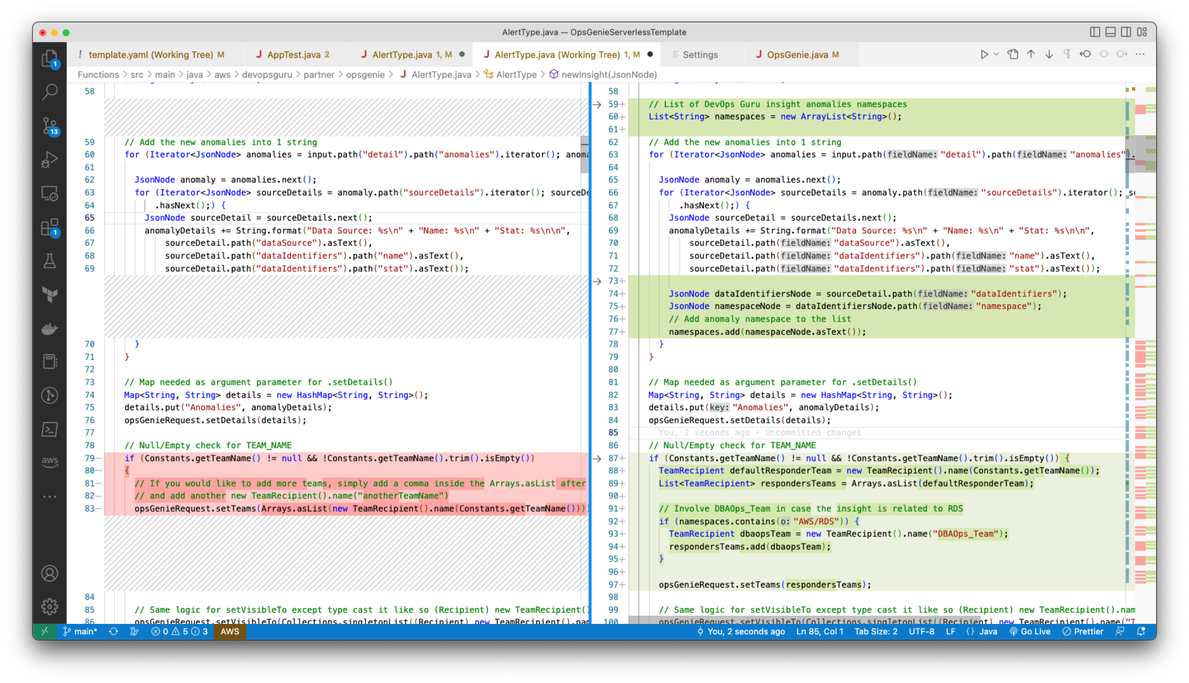
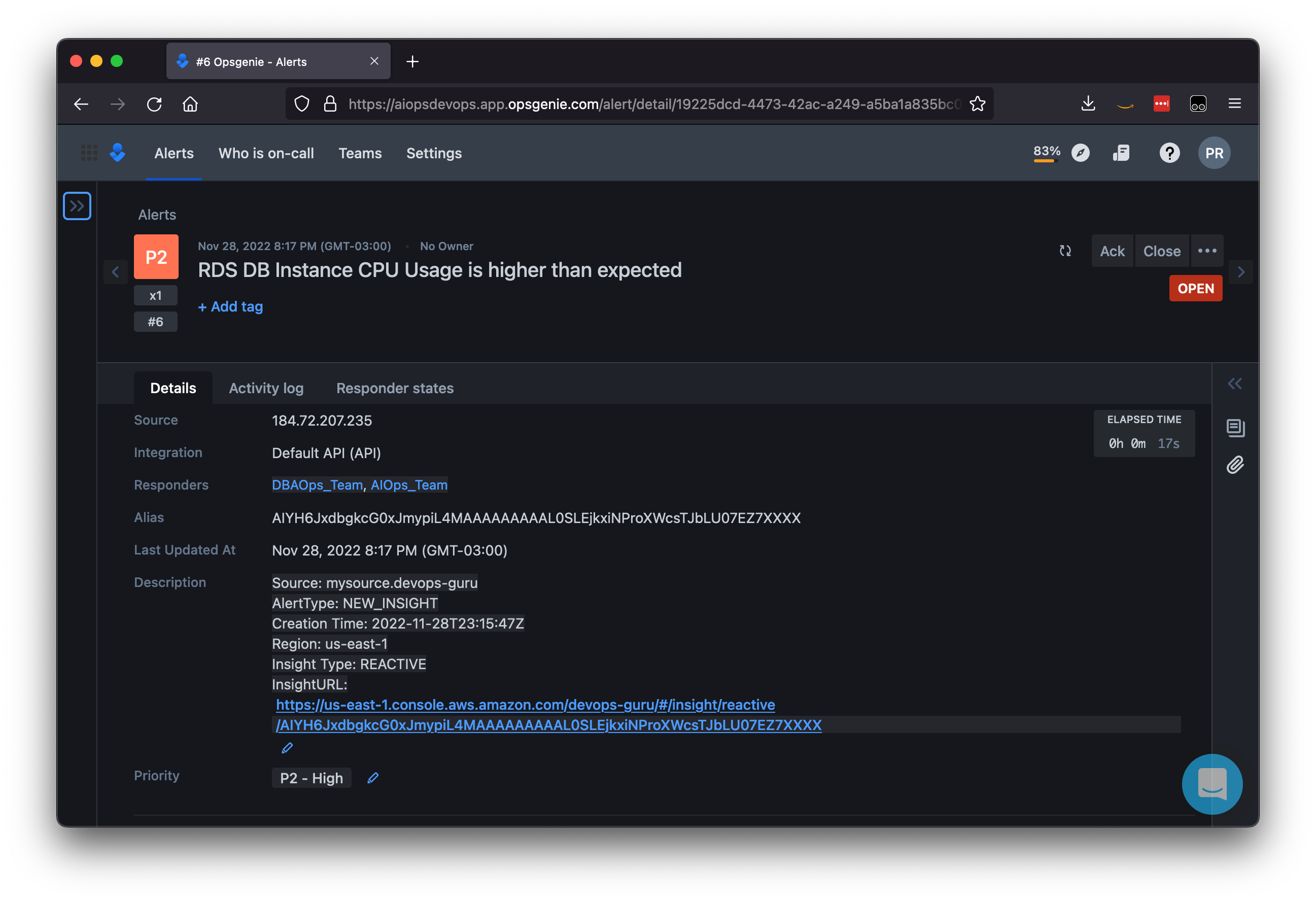

 Vidya Kotamraju is a Product Management Leader at Diligent, with close to 2 decades of experience leading award-winning B2B, B2C product and team success across multiple industries and geographies. Currently, she is focused on Diligent Highbond’s Data Automation Solutions.
 Tallis Hobbs is a Senior Software Engineer at Diligent. As a previous educator, he brings a unique skill set to the engineering space. He is passionate about the AWS serverless space and currently works on Diligent’s client facing Quicksight integration.
 Samit Kumbhani is a Sr. Solutions Architect at AWS based out of New York City area. Has has 18+ years of experience in building applications and focuses on Analytics, Business Intelligence and Databases. He enjoys working with customers to understand their challenges and solve them by creating innovative solutions using AWS services. Outside of work, Samit loves playing cricket, traveling and spending time with his family and friends.