Introducing native support for Apache Hudi, Delta Lake, and Apache Iceberg on AWS Glue for Apache Spark, Part 1: Getting Started

Post Syndicated from Akira Ajisaka original https://aws.amazon.com/blogs/big-data/part-1-getting-started-introducing-native-support-for-apache-hudi-delta-lake-and-apache-iceberg-on-aws-glue-for-apache-spark/

AWS Glue is a serverless, scalable data integration service that makes it easier to discover, prepare, move, and integrate data from multiple sources. AWS Glue provides an extensible architecture that enables users with different data processing use cases.

A common use case is building data lakes on Amazon Simple Storage Service (Amazon S3) using AWS Glue extract, transform, and load (ETL) jobs. Data lakes free you from proprietary data formats defined by the business intelligence (BI) tools and limited capacity of proprietary storage. In addition, data lakes help you break down data silos to maximize end-to-end data insights. As data lakes have grown in size and matured in usage, a significant amount of effort can be spent keeping the data up to date by ensuring files are updated in a transactionally consistent manner.

AWS Glue customers can now use the following open-source data lake storage frameworks: Apache Hudi, Linux Foundation Delta Lake, and Apache Iceberg. These data lake frameworks help you store data and interface data with your applications and frameworks. Although popular data file formats such as Apache Parquet, CSV, and JSON can store big data, data lake frameworks bundle distributed big data files into tabular structures that are otherwise hard to manage. This makes data lake table frameworks the building constructs of databases on data lakes.

We announced general availability for native support for Apache Hudi, Linux Foundation Delta Lake, and Apache Iceberg on AWS Glue for Spark. This feature removes the need to install a separate connector or associated dependencies, manage versions, and simplifies the configuration steps required to use these frameworks in AWS Glue for Apache Spark. With these open-source data lake frameworks, you can simplify incremental data processing in data lakes built on Amazon S3 by using ACID (atomicity, consistency, isolation, durability) transactions, upserts, and deletes.

This post demonstrates how AWS Glue for Apache Spark works with Hudi, Delta, and Iceberg dataset tables, and describes typical use cases on an AWS Glue Studio notebook.

Enable Hudi, Delta, Iceberg in Glue for Apache Spark

You can use Hudi, Delta, or Iceberg by specifying a new job parameter --datalake-formats. For example, if you want to use Hudi, you need to specify the key as --datalake-formats and the value as hudi. If the option is set, AWS Glue automatically adds the required JAR files into the runtime Java classpath, and that’s all you need. You don’t need to build and configure the required libraries or install a separate connector. You can use the following library versions with this option.

AWS Glue version Hudi Delta Lake Iceberg
AWS Glue 3.0 0.10.1 1.0.0 0.13.1
AWS Glue 4.0 0.12.1 2.1.0 1.0.0

If you want to use other versions of the preceding libraries, you can choose either of the following options:

If you choose either of the preceding options, you need to make sure the --datalake-formats job parameter is unspecified. For more information, see Process Apache Hudi, Delta Lake, Apache Iceberg datasets at scale, part 1: AWS Glue Studio Notebook.

Prerequisites

To continue this tutorial, you need to create the following AWS resources in advance:

Process Hudi, Delta, and Iceberg datasets on an AWS Glue Studio notebook

AWS Glue Studio notebooks provide serverless notebooks with minimal setup. It makes data engineers and developers quickly and interactively explore and process their datasets. You can start using Hudi, Delta, or Iceberg in an AWS Glue Studio notebook by specifying the parameter via %%configure magic and setting the AWS Glue version to 3.0 as follows:

# Use Glue version 3.0
%glue_version 3.0

# Configure '--datalake-formats' Job parameter
%%configure
{
  "--datalake-formats": "your_comma_separated_formats"
}

For more information, refer to the example notebooks available in the GitHub repository:

For this post, we use an Iceberg DataFrame as an example.

The following sections explain how to use an AWS Glue Studio notebook to create an Iceberg table and append records to the table.

Launch a Jupyter notebook to process Iceberg tables

Complete the following steps to launch an AWS Glue Studio notebook:

  1. Download the Jupyter notebook file.
  2. On the AWS Glue console, choose Jobs in the navigation plane.
  3. Under Create job, select Jupyter Notebook.

  1. Select Upload and edit an existing notebook.
  2. Upload native_iceberg_dataframe.ipynb through Choose file under File upload.

  1. Choose Create.
  2. For Job name, enter native_iceberg_dataframe.
  3. For IAM Role, choose your IAM role.
  4. Choose Start notebook job.

Prepare and configure SparkSession with Iceberg configuration

Complete the following steps to configure SparkSession to process Iceberg tables:

  1. Run the following cell.

You can see --datalake-formats iceberg is set by the %%configure Jupyter magic command. For more information about Jupyter magics, refer to Configuring AWS Glue interactive sessions for Jupyter and AWS Glue Studio notebooks.

  1. Provide your S3 bucket name and bucket prefix for your Iceberg table location in the following cell, and run it.

  1. Run the following cells to initialize SparkSession.

  1. Optionally, if you previously ran the notebook, you need to run the following cell to clean up existing resources.

Now you’re ready to create Iceberg tables using the notebook.

Create an Iceberg table

Complete the following steps to create an Iceberg table using the notebook:

  1. Run the following cell to create a DataFrame (df_products) to write.

If successful, you can see the following table.

  1. Run the following cell to create an Iceberg table using the DataFrame.

  1. Now you can read data from the Iceberg table by running the following cell.

Append records to the Iceberg table

Complete the following steps to append records to the Iceberg table:

  1. Run the following cell to create a DataFrame (df_products_appends) to append.

  1. Run the following cell to append the records to the table.

  1. Run the following cell to confirm that the preceding records are successfully appended to the table.

Clean up

To avoid incurring ongoing charges, clean up your resources:

  1. Run step 4 in the Prepare and configure SparkSession with Iceberg configuration section in this post to delete the table and underlying S3 objects.
  2. On the AWS Glue console, choose Jobs in the navigation plane.
  3. Select your job and on the Actions menu, choose Delete job(s).
  4. Choose Delete to confirm.

Considerations

With this capability, you have three different options to access Hudi, Delta, and Iceberg tables:

  • Spark DataFrames, for example spark.read.format("hudi").load("s3://path_to_data")
  • SparkSQL, for example SELECT * FROM table
  • GlueContext, for example create_data_frame.from_catalog, write_data_frame.from_catalog, getDataFrame, and writeDataFrame

Learn more in Using the Hudi framework in AWS Glue, Using the Delta Lake framework in AWS Glue, and Using the Iceberg framework in AWS Glue.

Delta Lake native integration works with the catalog tables created from native Delta Lake tables by AWS Glue crawlers. This integration does not depend on manifest files. For more information, refer to Introducing native Delta Lake table support with AWS Glue crawlers.

Conclusion

This post demonstrated how to process Apache Hudi, Delta Lake, Apache Iceberg datasets using AWS Glue for Apache Spark. You can integrate your data using those data lake formats easily without struggling with library dependency management.

In subsequent posts in this series, we’ll show you how you can use AWS Glue Studio to visually author your ETL jobs with simpler configuration and setup for these data lake formats, and how to use AWS Glue workflows to orchestrate data pipelines and automate ingestion into your data lakes on Amazon S3 with AWS Glue jobs. Stay tuned!

If you have comments or feedback, please leave them in the comments.


About the authors

Akira Ajisaka is a Senior Software Development Engineer on the AWS Glue team. He likes open-source software and distributed systems. In his spare time, he enjoys playing both arcade and console games.

Noritaka Sekiyama is a Principal Big Data Architect on the AWS Glue team. He is responsible for building software artifacts to help customers. In his spare time, he enjoys cycling with his new road bike.

Savio Dsouza is a Software Development Manager on the AWS Glue team. His teams work on building and innovating in distributed compute systems and frameworks, namely on Apache Spark.

The High Cost of Human Error In OT Systems

Post Syndicated from Rapid7 original https://blog.rapid7.com/2023/01/26/the-high-cost-of-human-error-in-ot-systems/

The High Cost of Human Error In OT Systems

In baseball, a mistake made by a player that could have easily been avoided is sometimes called an “unforced error.” An unforced error is not an official error (that is, they are not reflected in statistics), however, they can result in additional runs being scored, runners getting on base, and even games being lost. This applies in cyber security, as well. Threat actors use all sorts of nefarious tactics to target your networks, but they usually can’t succeed without some mistakes from your team.

Rapid7’s partner SCADAfence recently commissioned a survey of 3500 OT professionals. Among the findings, nearly 80% of respondents believe that human error presents the greatest risk for compromise to operational technology (OT) control systems. The survey also found that 83% of respondents believe that there is a significant shortfall in the number of skilled workers. This could contribute to the problem, since under-qualified or improperly trained security workers are more likely to make preventable errors.

Still, many organizations continue to ignore the extremely high potential costs of human error.

Real World Consequences

Last year, SCADAfence argued that an explosion at the Freeport LNG natural gas plant, which a Russian group claimed responsibility for, was actually caused by human error. The timing of the explosion, less than two months after a major maintenance upgrade, and several other factors appear to indicate that improper procedures and a lapse in adherence to company policies were the cause. This was later confirmed by the U.S. Pipeline and Hazardous Materials Safety Administration (PHMSA).

Another example is the Oldsmar Water Facility Attack in 2021. According to reports, human error played a large factor in the attack—in which hackers gained unauthorized access to the water facility’s industrial control system (ICS) network and increased sodium hydroxide content in drinking water to poisonous levels. The Oldsmar facility was using Windows 7, even though Microsoft had stopped supporting it a year earlier. All of Oldsmar’s employees shared the same password to access TeamViewer, a remote access software. And, the facility was connected directly to the internet without any type of firewall protection installed. All of these easily preventable factors contributed to the attacker’s ability to gain access to the facility.

Human error in OT systems can take different forms. As stated above, weak, outdated or duplicated passwords have led to any number of cyber security breaches. Firewalls, which are relied on to provide a first line of OT cyber security defense, are frequently misconfigured or improperly deployed by IT staff members. Finally, phishing attacks, a form of social engineering used by malicious actors to gain information from unwitting victims which is then used to access secure systems, are a major starting point for attacks on critical infrastructure.

Rapid7’s Advice

The number one way to prevent human error from leading to costly cyber attacks is training. OT and IT staff should be regularly trained on company security policies and should understand the importance of always following protocol. Also, teams need to work closely together to ensure that proper protections are in place across the network.
There are a number of best practices that have been shown to reduce the frequency and severity of cyber attacks in OT and ICS networks. Organizations should:

  • Require secure passwords that are changed on a regular schedule. Never allow team members to share passwords or access IDs to systems. Each employee that requires access to a system or device should have a unique user name and account.
  • Reduced access privilege access
  • Keep your network updated with important patches and upgrades
  • Make sure the tools your teams rely on are reliable, effective, and up to date.
  • Stay on top of news and information about newly discovered vulnerabilities, and potential threats relevant to your organization.

Finally, if your team lacks bandwidth or necessary skills, consider using managed services to gain insights and relevant threat information about your network.
This article was written in partnership with SCADAfence.

Visualize AWS WAF logs with an Amazon CloudWatch dashboard

Post Syndicated from Diana Alvarado original https://aws.amazon.com/blogs/security/visualize-aws-waf-logs-with-an-amazon-cloudwatch-dashboard/

AWS WAF is a web application firewall service that helps you protect your applications from common exploits that could affect your application’s availability and your security posture. One of the most useful ways to detect and respond to malicious web activity is to collect and analyze AWS WAF logs. You can perform this task conveniently by sending your AWS WAF logs to Amazon CloudWatch Logs and visualizing them through an Amazon CloudWatch dashboard.

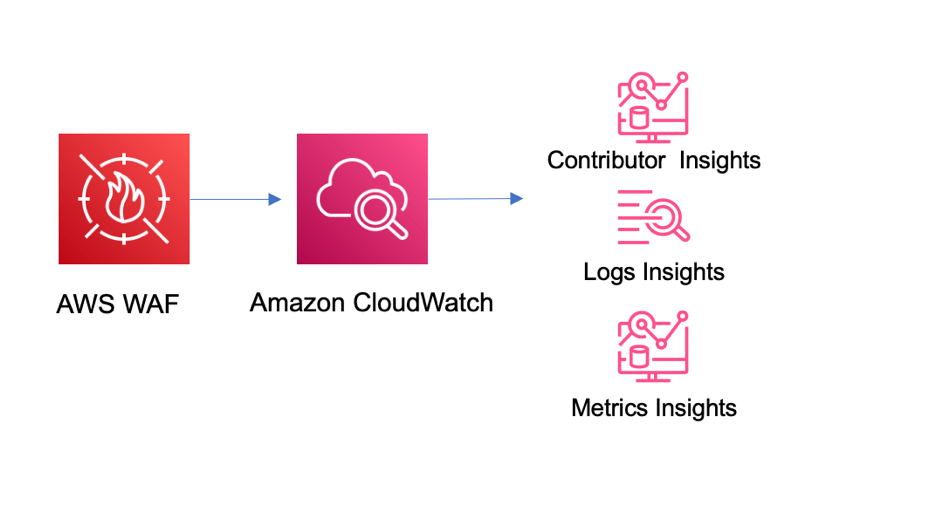
In this blog post, I’ll show you how to use Amazon CloudWatch to monitor and analyze AWS WAF activity using the options in CloudWatch metrics, Contributor Insights, and Logs Insights. I’ll also walk you through how to deploy this solution in your own AWS account by using an AWS CloudFormation template.

Prerequisites

This blog post builds on the concepts introduced in the blog post Analyzing AWS WAF Logs in Amazon CloudWatch Logs. There we introduced how to natively set up AWS WAF logging to Amazon CloudWatch logs, and discussed the basic options that are available for visualizing and analyzing the data provided in the logs.

The only AWS services that you need to turn on for this solution are Amazon CloudWatch and AWS WAF. The solution assumes that you’ve previously set up AWS WAF log delivery to Amazon CloudWatch Logs. If you have not done so, follow the instructions for AWS WAF logging destinations – CloudWatch Logs.

You will need to provide the following parameters for the CloudFormation template:

  • CloudWatch log group name for the AWS WAF logs
  • The AWS Region for the logs
  • The name of the AWS WAF web access control list (web ACL)

Solution overview

The architecture of the solution is outlined in Figure 1. The solution takes advantage of the native integration available between AWS WAF and CloudWatch, which simplifies the setup and management of this solution.

Figure 1: Solution architecture

Figure 1: Solution architecture

In the solution, the logs are sent to CloudWatch (when you enable log delivery). From there, they’re ready to be consumed by all the different service options that CloudWatch offers, including the ones that we’ll use in this solution: CloudWatch Logs Insights and Contributor Insights.

Deploy the solution

Choose the following Launch stack button to launch the CloudFormation stack in your account.

Launch Stack

You’ll be redirected to the CloudFormation service in the AWS US East (N. Virginia) Region, which is the default Region to deploy this solution, although this can vary depending on where your web ACL is located. You can change the Region as preferred. The template will spin up multiple cloud resources, such as the following:

  • CloudWatch Logs Insights queries
  • CloudWatch Contributor Insights visuals
  • CloudWatch dashboard

The solution is quickly deployed to your account and is ready to use in less than 30 minutes. You can use the solution when the status of the stack changes to CREATE_COMPLETE.

As a measure to control costs, you can also choose whether to create the Contributor Insights rules and enable them by default. For more information on costs, see the Cost considerations section later in this post.

Explore and validate the dashboard

When the CloudFormation stack is complete, you can choose the Output tab in the CloudFormation console and then choose the dashboard link. This will take you to the CloudWatch service in the AWS Management Console. The dashboard time range presents information for the last hour of activity by default, and can go up to one week, but keep in mind that Contributor Insights has a maximum time range of 24 hours. You can also select a different dashboard refresh interval from 10 seconds up to 15 minutes.

The dashboard provides the following information from CloudWatch.

Rule name Description
WAF_top_terminating_rules This rule shows the top rules where the requests are being terminated by AWS WAF. This can help you understand the main cause of blocked requests.
WAF_top_ips This rule shows the top source IPs for requests. This can help you understand if the traffic and activity that you see is spread across many IPs or concentrated in a small group of IPs.
WAF_top_countries This rule shows the main source countries for the IPs in the requests. This can help you visualize where the traffic is originating.
WAF_top_user_agents This rule shows the main user agents that are being used to generate the requests. This will help you isolate problematic devices or identify potential false positives.
WAF_top_uri This rule shows the main URIs in the requests that are being evaluated. This can help you identify if one specific path is the target of activity.
WAF_top_http This rule shows the HTTP methods used for the requests examined by AWS WAF. This can help you understand the pattern of behavior of the traffic.
WAF_top_referrer_hosts This rule shows the main referrer from which requests are being sent. This can help you identify incorrect or suspicious origins of requests based on the known application flow.
WAF_top_rate_rules This rule shows the main rate rules being applied to traffic. It helps understand volumetric activity identified by AWS WAF.
WAF_top_labels This rule shows the top labels found in logs. This can help you visualize the main rules that are matching on the requests evaluated by AWS WAF.

The dashboard also provides the following information from the default CloudWatch metrics sent by AWS WAF.

Rule name Description
AllowedvsBlockedRequests This metric shows the number of all blocked and allowed requests. This can help you understand the number of requests that AWS WAF is actively blocking.
Bot Requests vs non-Bot requests This visual shows the number of requests identified as bots versus non-bots (if you’re using AWS WAF Bot Control).
All Requests This metric shows the number of all requests, separated by bot and non-bot origin. This can help you understand all requests that AWS WAF is evaluating.
CountedRequests This metric shows the number of all counted requests. This can help you understand the requests that are matching a rule but not being blocked, and aid the decision of a configuration change during the testing phase.
CaptchaRequests This metric shows requests that go through the CAPTCHA rule.

Figure 2 shows an example of how the CloudWatch dashboard displays the data within this solution. You can rearrange and customize the elements within the dashboard as needed.

You can review each of the queries and rules deployed with this solution. You can also customize these baseline queries and rules to provide more detailed information or to add custom queries and rules to the solution code. For more information on how to build queries and use CloudWatch Logs and Contributor Insights, see the CloudWatch documentation.

Use the dashboard for monitoring

After you’ve set up the dashboard, you can monitor the activity of the sites that are protected by AWS WAF. If suspicious activity is reported, you can use the visuals to understand the traffic in more detail, and drive incident response actions as needed.

Let’s consider an example of how to use your new dashboard and its data to drive security operations decisions. Suppose that you have a website that sells custom clothing at a bargain price. It has a sign-up link to receive offers, and you’re getting reports of unusual activity by the application team. By looking at the metrics for the web ACL that protects the site, you can see the main country for source traffic and the contributing URIs, as shown in Figure 3. You can also see that most of the activity is being detected by rules that you have in place, so you can set the rules to block traffic, or if they are already blocking, you can just monitor the activity.

You can use the same visuals to decide whether an AWS WAF rule with high activity can be changed to autoblock suspicious web traffic without affecting valid customer traffic. By looking at the top terminating rules and cross-referencing information, such as source IPs, user agents, top URIs, and other request identifiers, you can understand the traffic pattern and activity of different applications and endpoints. From here, you can investigate further by using specific queries with CloudWatch Logs Insights.

Operational and security management with CloudWatch Logs Insights

You can use CloudWatch Logs Insights to interactively search and analyze log data in Amazon CloudWatch Logs using advanced queries to effectively investigate operational issues and security incidents.

Examine a bot reported as a false positive

You can use CloudWatch Logs Insights to identify requests that have specific labels to understand where the traffic is originating from based on source IP address and other essential event details. A simple example is investigating requests flagged as potential false positives.

Imagine that you have a reported false positive request that was flagged as a non-browser by AWS WAF Bot Control. You can run the non-browser user agent query that was created by the provided template on CloudWatch Logs Insights, as shown in the following example, and then verify the source IPs for the top hits for this rule group. Or you can look for a specific request that has been flagged as a false positive, in order to review the details and make adjustments as needed.

fields @timestamp, httpRequest.clientIp 
| filter @message like "awswaf:managed:aws:botcontrol:signal:non_browser_user_agent" 
| parse @message ""labels":[*]"as Labels 
| stats count(*) as requestCount by httpRequest.clientIP 
| display @timestamp,httpRequest.clientIp, httpRequest.uri,Labels 
| sort requestCount desc 
| limit 10

The non-browser user agent query also allows you confirm whether this request has other rule hits that were in count mode and were non-terminating; you can do this by examining the labels. If there are multiple rules matching the requests, that can be an indicator of suspicious activity.

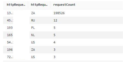
If you have a CAPTCHA challenge configured on the endpoint, you can also look at CAPTCHA responses. The CaptchaTokenqueryDefinition query provided in this solution uses a variation of the preceding format, and can display the main IPs from which bad tokens are being sent. An example query is shown following, along with the query results in Figure 4. If you have signals from non-browser user agents and CAPTCHA tokens missing, then that is a strong indicator of suspicious activity.

fields @timestamp, httpRequest.clientIp 
| filter captchaResponse.failureReason = "TOKEN_MISSING" 
| stats count(*) as requestCount by httpRequest.clientIp, httpRequest.country 
| sort requestCount desc 
| limit 10
Figure 4: Main IP addresses and number of counts for CAPTCHA responses

Figure 4: Main IP addresses and number of counts for CAPTCHA responses

This information can provide an indication of the main source of activity. You can then use other visuals, like top user agents or top referrers, to provide more context to the information and inform further actions, such as adding new rules to the AWS WAF configuration.

You can adapt the queries provided in the sample solution to other use cases by using the fields provided in the left-hand pane of CloudWatch Logs Insights.

Cost considerations

Configuring AWS WAF to send logs to Amazon CloudWatch logs doesn’t have an additional cost. The cost incurred is for the use of the CloudWatch features and services, such as log storage and retention, Contributor Insights rules enabled, Logs Insights queries run, matched log events, and CloudWatch dashboards. For detailed information on the pricing of these features, see the CloudWatch Logs pricing information. You can also get an estimate of potential costs by using the AWS pricing calculator for CloudWatch.

One way to help offset the cost of CloudWatch features and services is to restrict the use of the dashboard and enforce a log retention policy for AWS WAF that makes it cost effective. If you use the queries and monitoring only as-needed, this can also help reduce costs. By limiting the running of queries and the matched log events for the Contributor Insights rules, you can enable the rules only when you need them. AWS WAF also provides the option to filter the logs that are sent when logging is enabled. For more information, see AWS WAF log filtering.

Conclusion

In this post, you learned how to use a pre-built CloudWatch dashboard to monitor AWS WAF activity by using metrics and Contributor Insights rules. The dashboard can help you identify traffic patterns and activity, and you can use the sample Logs Insights queries to explore the log information in more detail and examine false positives and suspicious activity, for rule tuning.

For more information on AWS WAF and the features mentioned in this post, see the AWS WAF documentation.

If you have feedback about this post, submit comments in the Comments section below. If you have questions about this post, start a new thread on AWS WAF re:Post.

Want more AWS Security news? Follow us on Twitter.

Diana Alvarado

Diana Alvarado

Diana is Sr security solutions architect at AWS. She is passionate about helping customers solve difficult cloud challenges, she has a soft spot for all things logs.

Automate deployment and version updates for Amazon Kinesis Data Analytics applications with AWS CodePipeline

Post Syndicated from Anand Shah original https://aws.amazon.com/blogs/big-data/automate-deployment-and-version-updates-for-amazon-kinesis-data-analytics-applications-with-aws-codepipeline/

Amazon Kinesis Data Analytics is the easiest way to transform and analyze streaming data in real time using Apache Flink. Customers are already using Kinesis Data Analytics to perform real-time analytics on fast-moving data generated from data sources like IoT sensors, change data capture (CDC) events, gaming, social media, and many others. Apache Flink is a popular open-source framework and distributed processing engine for stateful computations over unbounded and bounded data streams.

Although building Apache Flink applications is typically the responsibility of a data engineering team, automating the deployment and provisioning infrastructure as code (IaC) is usually owned by the platform (or DevOps) team.

The following are typical responsibilities of the data engineering role:

  • Write code for real-time analytics Apache Flink applications
  • Roll out new application versions or roll them back (for example, in the case of a critical bug)

The following are typical responsibilities of the platform role:

  • Write code for IaC
  • Provision the required resources in the cloud and manage their access

In this post, we show how you can automate deployment and version updates for Kinesis Data Analytics applications and allow both Platform and engineering teams to effectively collaborate and co-own the final solution using AWS CodePipeline with the AWS Cloud Development Kit (AWS CDK).

Solution overview

To demonstrate the automated deployment and version update of a Kinesis Data Analytics application, we use the following example real-time data analytics architecture for this post.

Real-time data analytics architecture

The workflow includes the following steps:

  1. An AWS Lambda function (acting as data source) is the event producer pushing events on demand to Amazon Kinesis Data Streams when invoked.
  2. The Kinesis data stream receives and stores real-time events.
  3. The Kinesis Data Analytics application reads events from the data stream and performs real-time analytics on it.

Generic architecture

You can refer to the following generic architecture to adapt this example to your preferred CI/CD tool (for example, Jenkins). The overall deployment process is divided into three high-level parts:

  1. Infrastructure CI/CD – This portion is highlighted in orange. The infrastructure CI/CD pipeline is responsible for deploying all the real-time streaming architecture components, including the Kinesis Data Analytics application and any connected resources typically deployed using AWS CloudFormation.
  2. ApplicationStack – This portion is highlighted in gray. The application stack is deployed by the infrastructure CI/CD component using AWS CloudFormation.
  3. Application CI/CD – This portion is highlighted in green. The application CI/CD pipeline updates the Kinesis Data Analytics application in three steps:
    1. The pipeline builds the Java or Python source code of the Kinesis Data Analytics application and produces the application as a binary file.
    2. The pipeline pushes the latest binary file to the Amazon Simple Storage Service (Amazon S3) artifact bucket after a successful build as Kinesis Data Analytics application binary files are referenced from S3.
    3. The S3 bucket file put event triggers a Lambda function, which updates the version of the Kinesis Data Analytics application by deploying the latest binary.

The following diagram illustrates this workflow.

Workflow illustrated

CI/CD architecture with CodePipeline

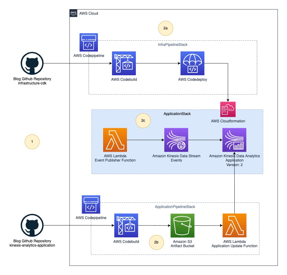
In this post, we implement the generic architecture using CodePipeline. The following diagram illustrates our updated architecture.

Updated architecture illustrated

The final solution includes the following steps:

  1. The platform (DevOps) team and data engineering team push their source code to their respective code repositories.
  2. CodePipeline deploys the whole infrastructure as three stacks:
    1. InfraPipelineStack – Contains a pipeline to deploy the overall infrastructure.
    2. ApplicationPipelineStack – Contains a pipeline to build and deploy Kinesis Data Analytics application binaries. In this post, we build a Java source using the JavaBuildPipeline AWS CDK construct. You can use the PythonBuildPipeline AWS CDK construct to build a Python source.
    3. ApplicationStack – Contains real-time data analytics pipeline resources including Lambda (data source), Kinesis Data Streams (storage), and Kinesis Data Analytics (Apache Flink application).

Deploy resources using AWS CDK

The following GitHub repository contains the AWS CDK code to create all the necessary resources for the data pipeline. This removes opportunities for manual error, increases efficiency, and ensures consistent configurations over time. To deploy the resources, complete the following steps:

  1. Clone the GitHub repository to your local computer using the following command:
git clone https://github.com/aws-samples/automate-deployment-and-version-update-of-kda-application
  1. Download and install the latest Node.js.
  2. Run the following command to install the latest version of AWS CDK:
npm install -g aws-cdk
  1. Run cdk bootstrap to initialize the AWS CDK environment in your AWS account. Replace your AWS account ID and Region before running the following command.
cdk bootstrap aws://123456789012/us-east-1

To learn more about the bootstrapping process, refer to Bootstrapping.

Part 1: Data engineering and platform teams push source code to their code repositories

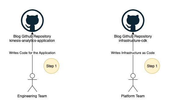
The data engineering and platform teams begin work in their respective code repositories, as illustrated in the following figure.

The data engineering and platform teams begin work in their respective code repositories, as illustrated in the following figure.

In this post, we use two folders instead of two GitHub repositories, which you can find under the root folder of the cloned repository:

  • kinesis-analytics-application – This folder contains example source code of the Kinesis Data Analytics application. This represents your Kinesis Data Analytics application source code developed by your data engineering team.
  • infrastructure-cdk – This folder contains example AWS CDK source code of the final solution used for provisioning all the required resources and CodePipeline. You can reuse this code for your Kinesis Data Analytics application deployment.

Application development teams usually stores the application source code in git repositories. For the demonstration purpose, we will use source code as zip file downloaded from Github instead of connecting CodePipeline to the Github repository. You may want to directly connect source repository with CodePipeline. To learn more about how to connect, refer to Create a connection to GitHub.

Part 2: The platform team deploys the application pipeline

The following figure illustrates the next step in the workflow.

Next step in the workflow illustrated

In this step, you deploy the first pipeline to build the Java source code from kinesis-analytics-application. Complete the following steps to deploy ApplicationPipelineStack:

  1. Open your terminal, bash, or command window depending on your OS.
  2. Switch the current path to the folder infrastructure-cdk.
  3. Run npm install to download all dependencies.
  4. Run cdk deploy ApplicationPipelineStack to deploy the application pipeline.

This process should take about 5 minutes to complete and deploys the following resources to your AWS account, highlighted in green in the preceding diagram:

  • CodePipeline, containing stages for AWS CodeBuild and AWS CodeDeploy
  • An S3 bucket to store binaries
  • A Lambda function to update the Kinesis Data Analytics application JAR after manual approval

Trigger an automatic build for the application pipeline

After the cdk deploy command is successful, complete the following steps to automatically run the pipeline:

  1. Download the source code .zip file.
  2. On the AWS CloudFormation console, choose Stacks in the navigation pane.
  3. Choose the stack ApplicationPipelineStack.Choose the stack ApplicationPipelineStack.
  4. On the Outputs tab, choose the link for the key ArtifactBucketLink.On the Outputs tab, choose the link for the key ArtifactBucketLink.

You’re redirected to the S3 artifact bucket.

  1. Choose Upload.
  2. Upload the source code .zip file you downloaded.

The first pipeline run (shown as Auto Build in the following diagram) starts automatically and takes about 5 minutes to reach the manual approval stage. The pipeline automatically downloads the source code from the artifact bucket, builds the Java project kinesis-analytics-application using Maven, and publishes the output binary JAR file back to the artifact bucket under the directory jars.

The pipeline automatically downloads the source code from the artifact bucket, builds the Java project kinesis-analytics-application using Maven, and publishes the output binary JAR file back to the artifact bucket under the directory jars.

View the application pipeline run

Complete the following steps to view the application pipeline run:

  1. On the AWS CloudFormation console, navigate to the stack ApplicationPipelineStack.
  2. On the Outputs tab, choose the link for the key ApplicationCodePipelineLink.On the Outputs tab, choose the link for the key ApplicationCodePipelineLink.

You’re redirected to the pipeline details page. You can see a detailed view of the pipeline, including the state of each action in each stage and the state of the transitions.

Do not approve the build for the manual approval stage yet; this is done later.

Part 3: The platform team deploys the infrastructure pipeline

The application pipeline run publishes a JAR file named kinesis-analytics-application-final.jar to the artifact bucket. Next, we deploy the Kinesis Data Analytics architecture. Complete the following steps to deploy the example flow:

  1. Open a terminal, bash, or command window depending on your OS.
  2. Switch the current path to the folder infrastructure-cdk.
  3. Run cdk deploy InfraPipelineStack to deploy the infrastructure pipeline.

This process should take about 5 minutes to complete and deploys a pipeline containing stages for CodeBuild and CodeDeploy to your AWS account, as highlighted in green in the following diagram.

This process should take about 5 minutes to complete and deploys a pipeline containing stages for CodeBuild and CodeDeploy to your AWS account, as highlighted in green in the following diagram.

When the cdk deploy is complete, the infrastructure pipeline run starts automatically (shown as Auto Build 1 in the following diagram) and takes about 10 minutes to download the source code from the artifact bucket, build the AWS CDK project infrastructure-stack, and deploy ApplicationStack automatically to your AWS account. When the infrastructure pipeline run is complete, the following resources are deployed to your account (shown in green in following diagram):

  • A CloudFormation template named app-ApplicationStack
  • A Lambda function acting as a data source
  • A Kinesis data stream acting as the stream storage
  • A Kinesis Data Analytics application with the first version of kinesis-analytics-application-final.jarWhen the infrastructure pipeline run is complete, the following resources are deployed to your account (shown in green in following diagram):

View the infrastructure pipeline run

Complete the following steps to view the application pipeline run:

  1. On the AWS CloudFormation console, navigate to the stack InfraPipelineStack.On the AWS CloudFormation console, navigate to the stack InfraPipelineStack.
  2. On the Outputs tab, choose the link for the key InfraCodePipelineLink.On the Outputs tab, choose the link for the key InfraCodePipelineLink.

You’re redirected to the pipeline details page. You can see a detailed view of the pipeline, including the state of each action in each stage and the state of the transitions.

Step 4: The data engineering team deploys the application

Now your account has everything in place for the data engineering team to work independently and roll out new versions of the Kinesis Data Analytics application. You can approve the respective application build from the application pipeline to deploy new versions of the application. The following diagram illustrates the full workflow.

Diagram illustrates the full workflow.

The build process starts automatically when it detects changes in the source code. You can test a version update by re-uploading the source code .zip file to the S3 artifact bucket. In a real-world use case, you update the main branch either via a pull request or by merging your changes, and this action triggers a new pipeline run automatically.

View the current application version

To view the current version of the Kinesis Data Analytics application, complete the following steps:

  1. On the AWS CloudFormation console, navigate to the stack InfraPipelineStack.
  2. On the Outputs tab, choose the link for the key KDAApplicationLink.On the Outputs tab, choose the link for the key KDAApplicationLink.

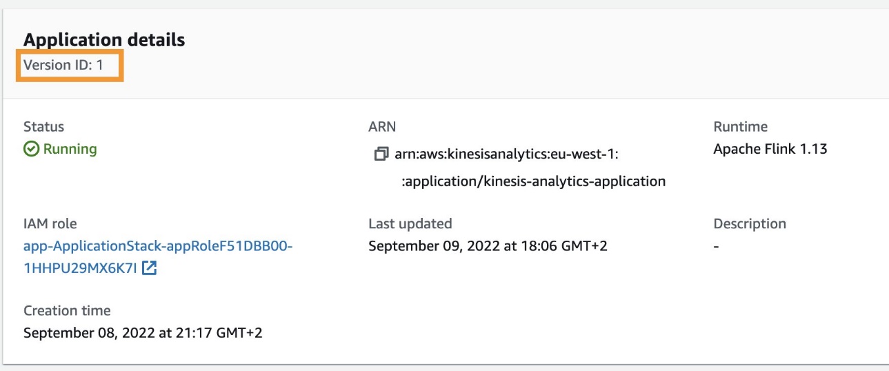
You’re redirected to the Kinesis Data Analytics application details page. You can find the current application version by looking at Version ID.

Find the current application version by looking at Version ID

Approve the application deployment

Complete the following steps to approve the deployment (or version update) of the Kinesis Data Analytics application:

  1. On the AWS CloudFormation console, navigate to the stack ApplicationPipelineStack.
  2. On the Outputs tab, choose the link for the key ApplicationCodePipelineLink.
  3. Choose Review from the pipeline approval stage.Choose Review from the pipeline approval stage
  4. When prompted, choose Approve to provide approval (optionally adding any comments) for the Kinesis Data Analytics application deployment or version update.Choose Approve to provide approval
  5. Repeat the steps mentioned earlier to view the current application version.

You should see the application version as defined in Version ID increased by one, as shown in the following screenshot.

Application version as defined in Version ID increased by one

Deploying a new version of the Kinesis Data Analytics application will cause a downtime of around 5 minutes because the Lambda function responsible for the version update makes the API call UpdateApplication, which restarts the application after updating the version. However, the application resumes stream processing where it left off after the restart.

Clean up

Complete the following steps to delete your resources and stop incurring costs:

  1. On the AWS CloudFormation console, select the stack InfraPipelineStack and choose Delete.
  2. Select the stack app-ApplicationStack and choose Delete.
  3. Select stack ApplicationPipelineStack and choose Delete.
  4. On the Amazon S3 console, select the bucket with the name starting with javaappCodePipeline and choose Empty.
  5. Enter permanently delete to confirm the choice.
  6. Select the bucket again and choose Delete.
  7. Confirm the action by entering the bucket name when prompted.
  8. Repeat these steps to delete the bucket with the name starting with infrapipelinestack-pipelineartifactsbucket.

Summary

This post demonstrated how to automate deployment and version updates for your Kinesis Data Analytics applications using CodePipeline and AWS CDK.

For more information, see Continuous integration and delivery (CI/CD) using CDK Pipelines and CodePipeline tutorials.


About the Author

About the AuthorAnand Shah is a Big Data Prototyping Solutions Architect at AWS. He works with AWS customers and their engineering teams to build prototypes using AWS analytics services and purpose-built databases. Anand helps customers solve the most challenging problems using the art of the possible technology. He enjoys beaches in his leisure time.

Backblaze vs. Dropbox: Backing Up Our Backup Claims

Post Syndicated from Stephanie Doyle original https://www.backblaze.com/blog/backblaze-vs-dropbox-backing-up-our-backup-claims/


If you follow the Backblaze blog, you’ve likely come across some of our “How to Back Up Your Life” posts. We’re interested in helping you, our readers, design the best backup plan for your needs, regardless of what your setup is, what social networks you’re on, or if you’re on a Mac or a PC.

Of course, Dropbox has shown up in that content. We have several articles talking about the best ways to integrate with their platform, and some articles that just talk about how to deal with the differences between sync and backup.

Recently, we heard that Dropbox released a backup product and wrote an article comparing our two services. (We’re flattered that they consider Backblaze to be the gold standard to compare to!) We thought we’d take this opportunity to respond, mostly because we want our library of guides to include their new offering, and a little bit because, well, there were some interesting interpretations included in the article.

Without further ado, our thoughts on the differences between Backblaze and Dropbox backup.

Backup vs. Sync

Dropbox started out as a syncing service, which, as we’ve noted before, is not the same as a backup service. When you’re using a sync service, you can easily delete or change a file, save it, and then lose the one you actually wanted to keep. This is one of the big reasons you should back up, even if your files are synced.

Over the past several years, Dropbox has been expanding their offerings, including file transfer, document signing, and now backup. It makes a lot of sense if you want to be a leading file management system. But, does Dropbox Backup stack up as a functional, independent product—or is it more of an add-on they’re offering to their sync functionality?

A Quick Note on Citing Your Sources…

When I set out to write this article, I first wanted to see if the things Dropbox claims hold water—After all, innovation is about iteration, and you don’t change or get better if you believe your product is perfect. Maybe we could learn something.

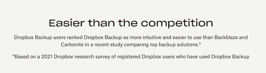
I kept hearing about this product research they’d done:

Source: Dropbox Backup vs. Backblaze.

You know we at Backblaze love data, so I was curious—How did they collect this data? Who were these users? I couldn’t find much more information about it in the article. But, after some digging, I found this on their product page:

Source: Dropbox Backup page.

It makes sense that people who already use Dropbox would like a product similar to the one they’re paying for. But, do the rest of the claims of the article hold true?

Let’s Talk Pricing

Hey, price is definitely a part of my decision when I purchase services, and I’m sure it’s part of yours too. So, let’s get the big argument out of the way first.

Backblaze Personal Backup is $7 per month. That license includes an automatic, set-it-and-forget-it backup service, unlimited data storage, 30-day version history, and you can add one-year version history for just $2 per month or forever version history for $2 per month plus $0.005 per GB for anything over 10GB.

For argument’s sake, let’s grant that Dropbox also built a backup product that runs smoothly in the background. I haven’t personally tried it, but I’ve used Dropbox for file management, and it’s a great service.

Dropbox Backup has several tiers of payment. It’s also included in many of their other paid plans—so, in other words, if you’re already paying $12–$90+ per month for Dropbox, you can take advantage of Dropbox Backup. But, if you’re trying to purchase just Dropbox Backup, there are several tiers of licensing, and (like most SaaS companies) there are discounts for paying monthly versus yearly.

So, let’s try to compare apples to apples here. Say you only have $10 per month budgeted for your backup plan. Here’s what you’d get with Dropbox:

  • Year-long commitment – so no flexibility to cancel
  • 2,000GB data cap
  • 30-day version history

For the same $10 per month, here’s what you’d get with Backblaze:

  • Monthly commitment – flexibility to cancel
  • No data cap
  • One-year version history

For reference, in 2020 most consumers were storing around 500GB of data in their personal storage clouds, but, unsurprisingly, we store more data every year. According to experts, data storage is doubling about every four years. So, you can certainly expect those “running out of space” notifications to be pushing you to upgrade your Dropbox service, and probably sooner than you’d expect.

Speaking of Flexibility

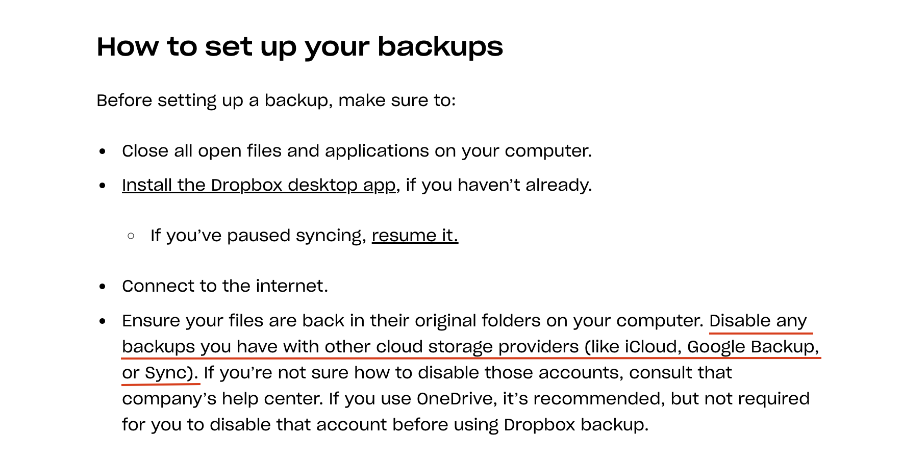
Once you check out Dropbox’s Help docs, there are a few other things to note. Essentially, if you want to use Dropbox Backup, you have to turn off other syncing and backup services (except for OneDrive).

Source: How to Use Dropbox Backup.

In order for Dropbox Backup to work, you have to turn off iCloud and Google Backup/Sync services, both of which are super compatible with your mobile devices and which many many folks rely on (two billion Google customers can’t be wrong). And, what about business use cases? Say you’re an enterprise client who wants to work in G-Suite—Dropbox Backup is not your answer. To put it simply: Dropbox Backup works best if Dropbox is the product you also use to store your files in the cloud.

Backblaze, on the other hand, works with whatever other services you’re rocking. Many of the choices we’ve made are reflective of that, including our restoration process. Dropbox offers restoration in place—if you use Dropbox to manage your files already. Basically, when you restore in place, you’re making a change to the virtual environment of your files (their copy of your hard drive that lives in Dropbox), and then they send that back to your computer. If you use a different syncing service or are accessing a file from another device, well, you’re going through the same download/restore process as every other backup service.

Restores for All

Here’s another thing: It’s a main point in Dropbox’s article that we offer recovery via USB. They turn their noses up at delivering files via the mail—Why would you wait for that?

Well, if you’ve lived in areas with not-great internet, dealt with being the family IT hero, or have a ton of data that needs to be moved, you know that having many ways to restore is key. Sure, it’s easy to scoff at all things analog, “OMG a USB drive via the mail?!” But an external drive (in this example, a USB) comes in super handy when you’re not tech savvy or have a ton of data to move—anyone who’s had to migrate lots of files (at work or at home) knows that sometimes the internet is not as fast as moving data via external devices.

Sure, there are tech reasons rapid ingest devices matter. But these guys matter too.

And, of course, you can always restore files from the internet with your Backblaze Personal Backup account. That’s our front-line method in our Help docs, and we’ve built a Download Manager to make things more seamless for our customers. We’ve made updates to our mobile apps, and just as importantly, we offer Backblaze B2 Storage Cloud and Backblaze Business Backup products. That means that if you ever outgrow our Personal Backup services, we’ve got you covered.

To Sum Up

We’re always happy there are more backup options for consumers. A little Backblaze flame warms our hearts when we know peoples’ data is backed up. Of course, we’d love it if everyone used Backblaze, but we want people to back up their data, even if it’s with a competitor.

If you’re already a paying Dropbox user, this may be a great option for you. But, if you’re like the majority of people and need something that works, no matter where/how you store your files or what other services you use, Backblaze Personal Backup is still your easy, affordable, and proven option.

The post Backblaze vs. Dropbox: Backing Up Our Backup Claims appeared first on Backblaze Blog | Cloud Storage & Cloud Backup.

[$] Reconsidering BPF ABI stability

Post Syndicated from original https://lwn.net/Articles/921088/

The BPF subsystem exposes many aspects of the kernel’s internal algorithms
and data structures; this naturally leads to concerns about maintaining
interface stability as the kernel changes. The longstanding position that
BPF offers no interface-stability guarantees to user space has always
seemed a little questionable; kernel developers have, in the past, found
themselves having to maintain interfaces that were not intended to be
stable. Now the BPF community is starting to think about what it might
mean to provide explicit stability promises for at least some of its
interfaces.

McKenney: What Does It Mean To Be An RCU Implementation?

Post Syndicated from original https://lwn.net/Articles/921351/

Paul McKenney looks at
a couple of Rust crates
in an attempt to determine whether they
actually implement the read-copy-update algorithm; in the process, he gives
an overview of the numerous RCU variants in the kernel.

Except that the first RCU crate, rcu_clean, throws a monkey wrench
into the works. It does not have any grace-period primitives, but
instead a clean() function that takes a reference to a
RCU-protected data item. The user invokes this at some point in
the code where it is known that there are no readers, either within
this thread or anywhere else. In true Rust fashion, in some cases,
the compiler is able to prove the presence or absence of readers
and issue a diagnostic when needed.

Security updates for Thursday

Post Syndicated from original https://lwn.net/Articles/921345/

Security updates have been issued by Debian (git), Fedora (libXpm and redis), Oracle (bind, firefox, grub2, java-1.8.0-openjdk, java-11-openjdk, kernel, libtasn1, libXpm, and sssd), Red Hat (thunderbird), SUSE (freeradius-server, kernel, libzypp-plugin-appdata, python-certifi, and xen), and Ubuntu (bind9, krb5, linux-raspi, linux-raspi-5.4, and privoxy).

Navigating the changing data localization landscape with Cloudflare’s Data Localization Suite

Post Syndicated from Emily Hancock original https://blog.cloudflare.com/dls-2022/

Navigating the changing data localization landscape with Cloudflare’s Data Localization Suite

Navigating the changing data localization landscape with Cloudflare’s Data Localization Suite

At Cloudflare, we believe that deploying effective cybersecurity measures is the best way to protect the privacy of personal information and can be more effective than making sure that information stays within a particular jurisdiction. Yet, we hear from customers in Europe, India, Australia, Japan, and many other regions that, as part of their privacy programs, they need solutions to localize data in order to meet their regulatory obligations.

So as we think about Data Privacy Day, which is coming up on January 28, we are in the interesting position of disagreeing with those who believe that data localization is a proxy for better data privacy, but of also wanting to support our customers who have to comply with certain regulations.

For this reason, we introduced our Data Localization Suite (DLS) in 2020 to help customers navigate a data protection landscape that focuses more and more on data localization. With the DLS, customers can use Cloudflare’s powerful global network and security measures to protect their businesses, while keeping the data we process on their behalf local. Since its launch, we’ve had many customers adopt the Data Localization Suite. In this blog post we want to share updates about how we’re making the DLS more comprehensive and easier to use.

The confusing state of data protection regulations

We frequently field questions from customers who hear about new local laws or interpretations of existing regulations that seem to limit what they can do with data. This is especially confusing for customers doing business on the global Internet because they have to navigate regulations that suggest customers based in one country can’t use products from companies based in another country, unless extensive measures are put in place.

We don’t think this is any way to regulate the Internet. As we’ll talk more about in our blog post tomorrow about cross-border data transfers, we’re encouraged to see new developments aimed at establishing a common set of data protections across jurisdictions to make these data transfers more seamless.

In the meantime, we have the Data Localization suite to help our customers navigate these challenges.

A recap of how the Data Localization Suite works

We developed DLS to address three primary customer concerns:

  1. How do I ensure my encryption keys stay in my jurisdiction?
  2. How can I ensure that application services like caching and WAF only run in my jurisdiction?
  3. How can I ensure that logs and metadata are never transferred outside my jurisdiction?

To address these concerns, our DLS has an encryption key component, a component that addresses where content in transit is terminated and inspected, and a component that keeps metadata within a customers’ jurisdiction:

1. Encryption Keys
Cloudflare has long offered Keyless SSL and Geo Key Manager, which ensure that private SSL/TLS key material never leaves the EU. Customers using our Geo Key Manager can choose for encryption keys to be stored only in data centers in the region the customer specifies. Keyless SSL ensures that Cloudflare never has possession of the private key material at all; Geo Key Manager ensures that keys are protected with cryptographic access control, so they can only be used in specified regions.

2. Regional Services:
Regional Services ensures that Cloudflare will only be able to decrypt and inspect the content of HTTPS traffic inside a customer’s chosen region. When Regional Services is enabled, regardless of which data center traffic first hits on our global network, rather than decrypting it at the first data center, we forward the TCP stream in encrypted form. Once it reaches a data center inside the customer’s chosen region, we decrypt and apply our Layer 7 security measures to prevent malicious traffic from reaching our customers’ websites.

3. Customer Metadata Boundary:
With this option enabled, no end user traffic logs (which contain IP addresses) that Cloudflare processes on behalf of our customers will leave the region chosen by the customer. (Currently only available only in the EU and US.)

Expanding Data Localization Suite to new regions

Although we launched the Data Localization Suite with Europe and America in mind at first, we quickly realized a lot of our customers were interested in versions specific to the Asia-Pacific region as well. In September of last year, we added support for Regional Services in Japan, Australia, and India.

Then in December 2022 we announced that Geo Key Manager is now accessible in 15 regions. Customers can both allow- and deny-list the regions that they want us to support for fine-grained control over where their key material is stored.

See also our technical deep dive about how we built Geo Key Manager v2.

Making data localization more accessible

Regional Services and the Customer Metadata Boundary offer important protections for our customers — but they’ve been too hard to use. Both have required manual steps taken by teams at Cloudflare, and have had confusing (or no) public APIs.

Today, we’re fixing that! We’re excited to announce two big improvements to usability:

  1. Regional Services customers now have a dedicated UI and API  for enabling Regional Services, accessible straight from the DNS tab. Different regions can now be set on a per-hostname basis
  2. Customers who want to use the Metadata Boundary can use our self-service API to enable it.

We’re excited about making it easier to use the Data Localization Suite and give customers more control over exactly how to localize which parts of their traffic.

What’s next

The Data Localization Suite is accessible today for enterprise customers. Please chat with your account representative if you’re interested in using it, and you can find more information here about configuring it in our developer docs.

We have lots more planned for the Data Localization Suite this year. We plan to support many more regions for Regional Services and the Metadata Boundary. We also plan to have full data localization support for all of our Zero Trust products. Stay tuned to the blog for more!

On Alec Baldwin’s Shooting

Post Syndicated from Bruce Schneier original https://www.schneier.com/blog/archives/2023/01/on-alec-baldwins-shooting.html

We recently learned that Alec Baldwin is being charged with involuntary manslaughter for his accidental shooting on a movie set. I don’t know the details of the case, nor the intricacies of the law, but I have a question about movie props.

Why was an actual gun used on the set? And why were actual bullets used on the set? Why wasn’t it a fake gun: plastic, or metal without a working barrel? Why does it have to fire blanks? Why can’t everyone just pretend, and let someone add the bang and the muzzle flash in post-production?

Movies are filled with fakery. The light sabers in Star Wars weren’t real; the lighting effects and “wooj-wooj” noises were add afterwards. The phasers in Star Trek weren’t real either. Jar Jar Binks was 100% computer generated. So were a gazillion “props” from the Harry Potter movies. Even regular, non-SF non-magical movies have special effects. They’re easy.

Why are guns different?

Scalable Annotation Service — Marken

Post Syndicated from Netflix Technology Blog original https://netflixtechblog.com/scalable-annotation-service-marken-f5ba9266d428

Scalable Annotation Service — Marken

by Varun Sekhri, Meenakshi Jindal

Introduction

At Netflix, we have hundreds of micro services each with its own data models or entities. For example, we have a service that stores a movie entity’s metadata or a service that stores metadata about images. All of these services at a later point want to annotate their objects or entities. Our team, Asset Management Platform, decided to create a generic service called Marken which allows any microservice at Netflix to annotate their entity.

Annotations

Sometimes people describe annotations as tags but that is a limited definition. In Marken, an annotation is a piece of metadata which can be attached to an object from any domain. There are many different kinds of annotations our client applications want to generate. A simple annotation, like below, would describe that a particular movie has violence.

  • Movie Entity with id 1234 has violence.

But there are more interesting cases where users want to store temporal (time-based) data or spatial data. In Pic 1 below, we have an example of an application which is used by editors to review their work. They want to change the color of gloves to rich black so they want to be able to mark up that area, in this case using a blue circle, and store a comment for it. This is a typical use case for a creative review application.

An example for storing both time and space based data would be an ML algorithm that can identify characters in a frame and wants to store the following for a video

  • In a particular frame (time)
  • In some area in image (space)
  • A character name (annotation data)
Pic 1 : Editors requesting changes by drawing shapes like the blue circle shown above.

Goals for Marken

We wanted to create an annotation service which will have the following goals.

  • Allows to annotate any entity. Teams should be able to define their data model for annotation.
  • Annotations can be versioned.
  • The service should be able to serve real-time, aka UI, applications so CRUD and search operations should be achieved with low latency.
  • All data should be also available for offline analytics in Hive/Iceberg.

Schema

Since the annotation service would be used by anyone at Netflix we had a need to support different data models for the annotation object. A data model in Marken can be described using schema — just like how we create schemas for database tables etc.

Our team, Asset Management Platform, owns a different service that has a json based DSL to describe the schema of a media asset. We extended this service to also describe the schema of an annotation object.

{
"type": "BOUNDING_BOX", ❶
"version": 0, ❷
"description": "Schema describing a bounding box",
"keys": {
"properties": { ❸
"boundingBox": {
"type": "bounding_box",
"mandatory": true
},
"boxTimeRange": {
"type": "time_range",
"mandatory": true
}
}
}
}

In the above example, the application wants to represent in a video a rectangular area which spans a range of time.

  1. Schema’s name is BOUNDING_BOX
  2. Schemas can have versions. This allows users to make add/remove properties in their data model. We don’t allow incompatible changes, for example, users can not change the data type of a property.
  3. The data stored is represented in the “properties” section. In this case, there are two properties
  4. boundingBox, with type “bounding_box”. This is basically a rectangular area.
  5. boxTimeRange, with type “time_range”. This allows us to specify start and end time for this annotation.

Geometry Objects

To represent spatial data in an annotation we used the Well Known Text (WKT) format. We support following objects

  • Point
  • Line
  • MultiLine
  • BoundingBox
  • LinearRing

Our model is extensible allowing us to easily add more geometry objects as needed.

Temporal Objects

Several applications have a requirement to store annotations for videos that have time in it. We allow applications to store time as frame numbers or nanoseconds.

To store data in frames clients must also store frames per second. We call this a SampleData with following components:

  • sampleNumber aka frame number
  • sampleNumerator
  • sampleDenominator

Annotation Object

Just like schema, an annotation object is also represented in JSON. Here is an example of annotation for BOUNDING_BOX which we discussed above.

{  
"annotationId": { ❶
"id": "188c5b05-e648-4707-bf85-dada805b8f87",
"version": "0"
},
"associatedId": { ❷
"entityType": "MOVIE_ID",
"id": "1234"
},
"annotationType": "ANNOTATION_BOUNDINGBOX", ❸
"annotationTypeVersion": 1,
"metadata": { ❹
"fileId": "identityOfSomeFile",
"boundingBox": {
"topLeftCoordinates": {
"x": 20,
"y": 30
},
"bottomRightCoordinates": {
"x": 40,
"y": 60
}
},
"boxTimeRange": {
"startTimeInNanoSec": 566280000000,
"endTimeInNanoSec": 567680000000
}
}
}
  1. The first component is the unique id of this annotation. An annotation is an immutable object so the identity of the annotation always includes a version. Whenever someone updates this annotation we automatically increment its version.
  2. An annotation must be associated with some entity which belongs to some microservice. In this case, this annotation was created for a movie with id “1234”
  3. We then specify the schema type of the annotation. In this case it is BOUNDING_BOX.
  4. Actual data is stored in the metadata section of json. Like we discussed above there is a bounding box and time range in nanoseconds.

Base schemas

Just like in Object Oriented Programming, our schema service allows schemas to be inherited from each other. This allows our clients to create an “is-a-type-of” relationship between schemas. Unlike Java, we support multiple inheritance as well.

We have several ML algorithms which scan Netflix media assets (images and videos) and create very interesting data for example identifying characters in frames or identifying match cuts. This data is then stored as annotations in our service.

As a platform service we created a set of base schemas to ease creating schemas for different ML algorithms. One base schema (TEMPORAL_SPATIAL_BASE) has the following optional properties. This base schema can be used by any derived schema and not limited to ML algorithms.

  • Temporal (time related data)
  • Spatial (geometry data)

And another one BASE_ALGORITHM_ANNOTATION which has the following optional properties which is typically used by ML algorithms.

  • label (String)
  • confidenceScore (double) — denotes the confidence of the generated data from the algorithm.
  • algorithmVersion (String) — version of the ML algorithm.

By using multiple inheritance, a typical ML algorithm schema derives from both TEMPORAL_SPATIAL_BASE and BASE_ALGORITHM_ANNOTATION schemas.

{
"type": "BASE_ALGORITHM_ANNOTATION",
"version": 0,
"description": "Base Schema for Algorithm based Annotations",
"keys": {
"properties": {
"confidenceScore": {
"type": "decimal",
"mandatory": false,
"description": "Confidence Score",
},
"label": {
"type": "string",
"mandatory": false,
"description": "Annotation Tag",
},
"algorithmVersion": {
"type": "string",
"description": "Algorithm Version"
}
}
}
}

Architecture

Given the goals of the service we had to keep following in mind.

  • Our service will be used by a lot of internal UI applications hence the latency for CRUD and search operations must be low.
  • Besides applications we will have ML algorithm data stored. Some of this data can be on the frame level for videos. So the amount of data stored can be large. The databases we pick should be able to scale horizontally.
  • We also anticipated that the service will have high RPS.

Some other goals came from search requirements.

  • Ability to search the temporal and spatial data.
  • Ability to search with different associated and additional associated Ids as described in our Annotation Object data model.
  • Full text searches on many different fields in the Annotation Object
  • Stem search support

As time progressed the requirements for search only increased and we will discuss these requirements in detail in a different section.

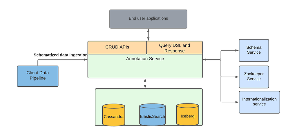
Given the requirements and the expertise in our team we decided to choose Cassandra as the source of truth for storing annotations. For supporting different search requirements we chose ElasticSearch. Besides to support various features we have bunch of internal auxiliary services for eg. zookeeper service, internationalization service etc.

Marken architecture

Above picture represents the block diagram of the architecture for our service. On the left we show data pipelines which are created by several of our client teams to automatically ingest new data into our service. The most important of such a data pipeline is created by the Machine Learning team.

One of the key initiatives at Netflix, Media Search Platform, now uses Marken to store annotations and perform various searches explained below. Our architecture makes it possible to easily onboard and ingest data from Media algorithms. This data is used by various teams for eg. creators of promotional media (aka trailers, banner images) to improve their workflows.

Search

Success of Annotation Service (data labels) depends on the effective search of those labels without knowing much of input algorithms details. As mentioned above, we use the base schemas for every new annotation type (depending on the algorithm) indexed into the service. This helps our clients to search across the different annotation types consistently. Annotations can be searched either by simply data labels or with more added filters like movie id.

We have defined a custom query DSL to support searching, sorting and grouping of the annotation results. Different types of search queries are supported using the Elasticsearch as a backend search engine.

  • Full Text Search — Clients may not know the exact labels created by the ML algorithms. As an example, the label can be ‘shower curtain’. With full text search, clients can find the annotation by searching using label ‘curtain’ . We also support fuzzy search on the label values. For example, if the clients want to search ‘curtain’ but they wrongly typed ‘curtian` — annotation with the ‘curtain’ label will be returned.
  • Stem Search — With global Netflix content supported in different languages, our clients have the requirement to support stem search for different languages. Marken service contains subtitles for a full catalog of titles in Netflix which can be in many different languages. As an example for stem search , `clothing` and `clothes` can be stemmed to the same root word `cloth`. We use ElasticSearch to support stem search for 34 different languages.
  • Temporal Annotations Search — Annotations for videos are more relevant if it is defined along with the temporal (time range with start and end time) information. Time range within video is also mapped to the frame numbers. We support labels search for the temporal annotations within the provided time range/frame number also.
  • Spatial Annotation Search — Annotations for video or image can also include the spatial information. For example a bounding box which defines the location of the labeled object in the annotation.
  • Temporal and Spatial Search — Annotation for video can have both time range and spatial coordinates. Hence, we support queries which can search annotations within the provided time range and spatial coordinates range.
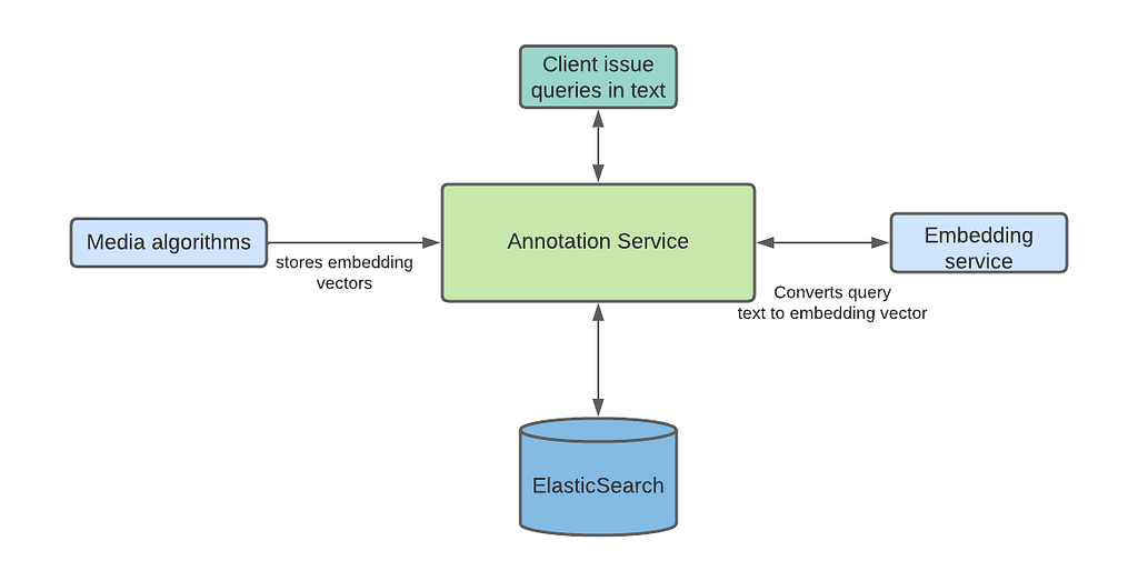
  • Semantics Search — Annotations can be searched after understanding the intent of the user provided query. This type of search provides results based on the conceptually similar matches to the text in the query, unlike the traditional tag based search which is expected to be exact keyword matches with the annotation labels. ML algorithms also ingest annotations with vectors instead of actual labels to support this type of search. User provided text is converted into a vector using the same ML model, and then search is performed with the converted text-to-vector to find the closest vectors with the searched vector. Based on the clients feedback, such searches provide more relevant results and don’t return empty results in case there are no annotations which exactly match to the user provided query labels. We support semantic search using Open Distro for ElasticSearch . We will cover more details on Semantic Search support in a future blog article.
Semantic search
  • Range Intersection — We recently started supporting the range intersection queries across multiple annotation types for a specific title in the real time. This allows the clients to search with multiple data labels (resulted from different algorithms so they are different annotation types) within video specific time range or the complete video, and get the list of time ranges or frames where the provided set of data labels are present. A common example of this query is to find the `James in the indoor shot drinking wine`. For such queries, the query processor finds the results of both data labels (James, Indoor shot) and vector search (drinking wine); and then finds the intersection of resulting frames in-memory.

Search Latency

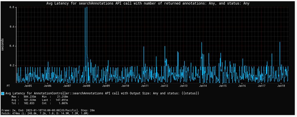
Our client applications are studio UI applications so they expect low latency for the search queries. As highlighted above, we support such queries using Elasticsearch. To keep the latency low, we have to make sure that all the annotation indices are balanced, and hotspot is not created with any algorithm backfill data ingestion for the older movies. We followed the rollover indices strategy to avoid such hotspots (as described in our blog for asset management application) in the cluster which can cause spikes in the cpu utilization and slow down the query response. Search latency for the generic text queries are in milliseconds. Semantic search queries have comparatively higher latency than generic text searches. Following graph shows the average search latency for generic search and semantic search (including KNN and ANN search) latencies.

Average search latency
Semantic search latency

Scaling

One of the key challenges while designing the annotation service is to handle the scaling requirements with the growing Netflix movie catalog and ML algorithms. Video content analysis plays a crucial role in the utilization of the content across the studio applications in the movie production or promotion. We expect the algorithm types to grow widely in the coming years. With the growing number of annotations and its usage across the studio applications, prioritizing scalability becomes essential.

Data ingestions from the ML data pipelines are generally in bulk specifically when a new algorithm is designed and annotations are generated for the full catalog. We have set up a different stack (fleet of instances) to control the data ingestion flow and hence provide consistent search latency to our consumers. In this stack, we are controlling the write throughput to our backend databases using Java threadpool configurations.

Cassandra and Elasticsearch backend databases support horizontal scaling of the service with growing data size and queries. We started with a 12 nodes cassandra cluster, and scaled up to 24 nodes to support current data size. This year, annotations are added approximately for the Netflix full catalog. Some titles have more than 3M annotations (most of them are related to subtitles). Currently the service has around 1.9 billion annotations with data size of 2.6TB.

Analytics

Annotations can be searched in bulk across multiple annotation types to build data facts for a title or across multiple titles. For such use cases, we persist all the annotation data in iceberg tables so that annotations can be queried in bulk with different dimensions without impacting the real time applications CRUD operations latency.

One of the common use cases is when the media algorithm teams read subtitle data in different languages (annotations containing subtitles on a per frame basis) in bulk so that they can refine the ML models they have created.

Future work

There is a lot of interesting future work in this area.

  1. Our data footprint keeps increasing with time. Several times we have data from algorithms which are revised and annotations related to the new version are more accurate and in-use. So we need to do cleanups for large amounts of data without affecting the service.
  2. Intersection queries over a large scale of data and returning results with low latency is an area where we want to invest more time.

Acknowledgements

Burak Bacioglu and other members of the Asset Management Platform contributed in the design and development of Marken.


Scalable Annotation Service — Marken was originally published in Netflix TechBlog on Medium, where people are continuing the conversation by highlighting and responding to this story.

How to run AWS CloudHSM workloads in container environments

Post Syndicated from Derek Tumulak original https://aws.amazon.com/blogs/security/how-to-run-aws-cloudhsm-workloads-on-docker-containers/

January 25, 2023: We updated this post to reflect the fact that CloudHSM SDK3 does not support serverless environments and we strongly recommend deploying SDK5.


AWS CloudHSM provides hardware security modules (HSMs) in the AWS Cloud. With CloudHSM, you can generate and use your own encryption keys in the AWS Cloud, and manage your keys by using FIPS 140-2 Level 3 validated HSMs. Your HSMs are part of a CloudHSM cluster. CloudHSM automatically manages synchronization, high availability, and failover within a cluster.

CloudHSM is part of the AWS Cryptography suite of services, which also includes AWS Key Management Service (AWS KMS), AWS Secrets Manager, and AWS Private Certificate Authority (AWS Private CA). AWS KMS, Secrets Manager, and AWS Private CA are fully managed services that are convenient to use and integrate. You’ll generally use CloudHSM only if your workload requires single-tenant HSMs under your own control, or if you need cryptographic algorithms or interfaces that aren’t available in the fully managed alternatives.

CloudHSM offers several options for you to connect your application to your HSMs, including PKCS#11, Java Cryptography Extensions (JCE), OpenSSL Dynamic Engine, or Microsoft Cryptography API: Next Generation (CNG). Regardless of which library you choose, you’ll use the CloudHSM client to connect to HSMs in your cluster.

In this blog post, I’ll show you how to use Docker to develop, deploy, and run applications by using the CloudHSM SDK, and how to manage and orchestrate workloads by using tools and services like Amazon Elastic Container Service (Amazon ECS), Kubernetes, Amazon Elastic Kubernetes Service (Amazon EKS), and Jenkins.

Solution overview

This solution demonstrates how to create a Docker container that uses the CloudHSM JCE SDK to generate a key and use it to encrypt and decrypt data.

Note: In this example, you must manually enter the crypto user (CU) credentials as environment variables when you run the container. For production workloads, you’ll need to consider how to secure and automate the handling and distribution of these credentials. You should work with your security or compliance officer to ensure that you’re using an appropriate method of securing HSM login credentials. For more information on securing credentials, see AWS Secrets Manager.

Figure 1 shows the solution architecture. The Java application, running in a Docker container, integrates with JCE and communicates with CloudHSM instances in a CloudHSM cluster through HSM elastic network interfaces (ENIs). The Docker container runs in an EC2 instance, and access to the HSM ENIs is controlled with a security group.

Figure 1: Architecture diagram

Figure 1: Architecture diagram

Prerequisites

To implement this solution, you need to have working knowledge of the following items:

  • CloudHSM
  • Docker 20.10.17 – used at the time of this post
  • Java 8 or Java 11 – supported at the time of this post
  • Maven 3.05 – used at the time of this post

Here’s what you’ll need to follow along with my example:

  1. An active CloudHSM cluster with at least one active HSM instance. You can follow the CloudHSM getting started guide to create, initialize, and activate a CloudHSM cluster.

    Note: For a production cluster, you should have at least two active HSM instances spread across Availability Zones in the Region.

  2. An Amazon Linux 2 EC2 instance in the same virtual private cloud (VPC) in which you created your CloudHSM cluster. The Amazon Elastic Compute Cloud (Amazon EC2) instance must have the CloudHSM cluster security group attached—this security group is automatically created during the cluster initialization and is used to control network access to the HSMs. To learn about attaching security groups to allow EC2 instances to connect to your HSMs, see Create a cluster in the AWS CloudHSM User Guide.
  3. A CloudHSM crypto user (CU) account. You can create a CU by following the steps in the topic Managing HSM users in AWS CloudHSM in the AWS CloudHSM User Guide.

Solution details

In this section, I’ll walk you through how to download, configure, compile, and run a solution in Docker.

To set up Docker and run the application that encrypts and decrypts data with a key in AWS CloudHSM

  1. On your Amazon Linux EC2 instance, install Docker by running the following command.

    # sudo yum -y install docker

  2. Start the docker service.

    # sudo service docker start

  3. Create a new directory and move to it. In my example, I use a directory named cloudhsm_container. You’ll use the new directory to configure the Docker image.

    # mkdir cloudhsm_container
    # cd cloudhsm_container

  4. Copy the CloudHSM cluster’s trust anchor certificate (customerCA.crt) to the directory that you just created. You can find the trust anchor certificate on a working CloudHSM client instance under the path /opt/cloudhsm/etc/customerCA.crt. The certificate is created during initialization of the CloudHSM cluster and is required to connect to the CloudHSM cluster. This enables our application to validate that the certificate presented by the CloudHSM cluster was signed by our trust anchor certificate.
  5. In your new directory (cloudhsm_container), create a new file with the name run_sample.sh that includes the following contents. The script runs the Java class that is used to generate an Advanced Encryption Standard (AES) key to encrypt and decrypt your data.
    #! /bin/bash
    
    # start application
    echo -e "\n* Entering AES GCM encrypt/decrypt sample in Docker ... \n"
    
    java -ea -jar target/assembly/aesgcm-runner.jar -method environment
    
    echo -e "\n* Exiting AES GCM encrypt/decrypt sample in Docker ... \n"

  6. In the new directory, create another new file and name it Dockerfile (with no extension). This file will specify that the Docker image is built with the following components:
    • The CloudHSM client package.
    • The CloudHSM Java JCE package.
    • OpenJDK 1.8 (Java 8). This is needed to compile and run the Java classes and JAR files.
    • Maven, a build automation tool that is needed to assist with building the Java classes and JAR files.
    • The AWS CloudHSM Java JCE samples that will be downloaded and built as part of the solution.
  7. Cut and paste the following contents into Dockerfile.

    Note: You will need to customize your Dockerfile, as follows:

    • Make sure to specify the SDK version to replace the one specified in the pom.xml file in the sample code. As of the writing of this post, the most current version is 5.7.0. To find the SDK version, follow the steps in the topic Check your client SDK version. For more information, see the Building section in the README file for the Cloud HSM JCE examples.
    • Make sure to update the HSM_IP line with the IP of an HSM in your CloudHSM cluster. You can get your HSM IPs from the CloudHSM console, or by running the describe-clusters AWS CLI command.
      	# Use the amazon linux image
      	FROM amazonlinux:2
      
      	# Pass HSM IP address as a build argument
      	ARG HSM_IP
      
      	# Install CloudHSM client
      	RUN yum install -y https://s3.amazonaws.com/cloudhsmv2-software/CloudHsmClient/EL7/cloudhsm-jce-latest.el7.x86_64.rpm
      
      	# Install Java, Maven, wget, unzip and ncurses-compat-libs
      	RUN yum install -y java maven wget unzip ncurses-compat-libs
              
      	# Create a work dir
      	WORKDIR /app
              
      	# Download sample code
      	RUN wget https://github.com/aws-samples/aws-cloudhsm-jce-examples/archive/refs/heads/sdk5.zip
              
      	# unzip sample code
      	RUN unzip sdk5.zip
             
      	# Change to the create directory
      	WORKDIR aws-cloudhsm-jce-examples-sdk5
      
      # Build JAR files using the installed CloudHSM JCE Provider version
      RUN export CLOUDHSM_CLIENT_VERSION=`rpm -qi cloudhsm-jce | awk -F': ' '/Version/ {print $2}'` \
              && mvn validate -DcloudhsmVersion=$CLOUDHSM_CLIENT_VERSION \
              && mvn clean package -DcloudhsmVersion=$CLOUDHSM_CLIENT_VERSION
              
        # Configure cloudhsm-client
        COPY customerCA.crt /opt/cloudhsm/etc/
        RUN /opt/cloudhsm/bin/configure-jce -a $HSM_IP
             
        # Copy the run_sample.sh script
        COPY run_sample.sh .
              
        # Run the script
        CMD ["bash","run_sample.sh"]

  8. Now you’re ready to build the Docker image. Run the following command, with the name jce_sample. This command will let you use the Dockerfile that you created in step 6 to create the image.

    # sudo docker build --build-arg HSM_IP=”<your HSM IP address>” -t jce_sample .

  9. To run a Docker container from the Docker image that you just created, run the following command. Make sure to replace the user and password with your actual CU username and password. (If you need help setting up your CU credentials, see prerequisite 3. For more information on how to provide CU credentials to the AWS CloudHSM Java JCE Library, see Providing credentials to the JCE provider in the CloudHSM User Guide).

    # sudo docker run --env HSM_USER=<user> --env HSM_PASSWORD=<password> jce_sample

    If successful, the output should look like this:

    	* Entering AES GCM encrypt/decrypt sample in Docker ... 
    
    	737F92D1B7346267D329C16E
    	Successful decryption
    
    	* Exiting AES GCM encrypt/decrypt sample in Docker ...

Conclusion

This solution provides an example of how to run CloudHSM client workloads in Docker containers. You can use the solution as a reference to implement your cryptographic application in a way that benefits from the high availability and load balancing built in to CloudHSM without compromising the flexibility that Docker provides for developing, deploying, and running applications.

If you have comments about this post, submit them in the Comments section below.

Want more AWS Security how-to content, news, and feature announcements? Follow us on Twitter.

Derek Tumulak

Derek Tumulak

Derek joined AWS in May 2021 as a Principal Product Manager. He is a data protection and cybersecurity expert who is enthusiastic about assisting customers with a wide range of sophisticated use cases.

Super-charged pivot tables in Amazon QuickSight

Post Syndicated from Bhupinder Chadha original https://aws.amazon.com/blogs/big-data/super-charged-pivot-tables-in-amazon-quicksight/

Amazon QuickSight is a fast and cloud-powered business intelligence (BI) service that makes it easy to create and deliver insights to everyone in your organization without any servers or infrastructure. QuickSight dashboards can also be embedded into applications and portals to deliver insights to external stakeholders. Additionally, with Amazon QuickSight Q, end-users can simply ask questions in natural language to get machine learning (ML)-powered visual responses to their questions.

Recently, Amazon FinTech migrated all their financial reporting to QuickSight. This involved migrating complex tables and pivot tables, helping them slice and dice large datasets and deliver pixel-perfect views of their data to their stakeholders. Amazon FinTech, like all QuickSight customers, needs fast performance on very large pivot tables in order to drive adoption of their dashboards. We have specifically launched two new features focused on scaling our pivot tables with the following improvements:

  • Faster loading of pivot tables during expand and collapse operations
  • Increased field limits for rows, columns, and values

In this post, we discuss these improvements to pivot tables in QuickSight.

Blazing fast pivot tables during expand and collapse operations

Today, QuickSight pivot tables work as an infinite load. As users scroll vertically or horizontally on the visual, new queries are run to fetch additional rows and columns of data with fixed row and column configurations for every query request.

For example, in the following table, we would load all carrier/city combinations nested under Dec 7, 2014 before we can continue querying the next date. Let’s say we have more than 500 carrier/city rows for a specific date; this will take more than a single query to get to the next date. The count of queries run depends on the cardinality of the dimension used in the pivot table.

In the following example of a collapsed pivot table, since the reader doesn’t see anything beyond the flight dates, having all carrier/city rows doesn’t change what is actively displayed on the pivot table. Even though individual SQL queries can be fast, users can perceive this table to load slowly due to the sheer number of queries being fired to load the hidden (collapsed) data. Therefore, loading every single row up to the Destination City field isn’t very useful when the pivot table in the collapsed state.

Therefore, to make our pivot tables load faster, we now only fetch the data for visible fields (expanded fields) along with a small subset of values under the collapsed field. This makes sure that data fetched in every new query is used to render new values that can be displayed immediately. We have seen customers improve their load time from 2–10 times faster depending on the complexity of their dataset.

This new behavior is automatically enabled, without requiring users to do anything on their side. Please note that while we plan to support all kinds of pivot tables to use this optimization, our current rollout only includes pivot tables with only row or only column fields not sorted by any metric.

Increased field limits for pivot tables

With the ever-growing depth and granularity of data being collected, our customers asked us to increase the number of fields and data points they can display in their visuals. We have been actively listening to your needs, and just like supporting more data points in line charts, we now are increasing our field limits for pivot tables.

The value field well limits have been increased from 20 to 40, and rows and columns have been increased from 20 each to a combined limit of 40. For example, if the user has 34 fields in rows, then they can add up to 6 fields to the column field well.

This will help unblock use cases requiring increased limits such as:

  • Metrics reporting – Monthly and weekly business reporting often requires having dozens of metrics presented in tabular formats. With the updated limits, you can display detailed, robust financial reports in a single pivot table rather than having to split it across multiple pivot tables.
  • Migration from legacy BI and reporting tools – Existing reports in these legacy systems require displaying and slicing across a large number of row hierarchies, for example a cost center expense analysis.
  • Custom use cases – These are specific industry and organization use cases where you can add dozens of values and row fields to display additional attributes. For example, a customer 360 report sliced by different regions.

As soon as you hit the limit, you receive an error message to indicate that the limit has been reached for that field well. For more details, refer to here.

Get started and stay updated!

Learn more about our new features in our newly launched QuickSight community’s Announcement section and supercharge your dashboards with the latest features from QuickSight!


About the authors

Bhupinder Chadha is a senior product manager for Amazon QuickSight focused on visualization and front end experiences. He is passionate about BI, data visualization and low-code/no-code experiences. Prior to QuickSight he was the lead product manager for Inforiver, responsible for building a enterprise BI product from ground up. Bhupinder started his career in presales, followed by a small gig in consulting and then PM for xViz, an add on visualization product.

Igal Mizrahi is a Senior Software Engineer for AWS QuickSight Charting team. He has been part of the team for the past 3 years, and previously worked on Amazon’s mobile shopping application for 4 years.

[$] X clients and byte swapping

Post Syndicated from original https://lwn.net/Articles/921196/

While there are still systems with both byte orders,
little-endian has
largely “won” the battle at this point since the vast majority of today’s
systems store data with the least-significant byte first (at the lowest
address). But when the X11 protocol was developed in the 1980s, there were
lots of systems of each byte order, so the X protocol allowed either order
and the server (display side) would swap the bytes to its byte order as
needed. Over time,
the code for swapping data in the messages, which was written in a
more-trusting era, has bit-rotted so that it is now a
largely untested attack surface that is nearly always unused. Peter
Hutterer has been doing some work to stop using that code by default, both
in upstream
X.org code and in downstream Fedora.

The collective thoughts of the interwebz