What’s life without a little WordPress exploitation? Courtesy of Hacker5preme (aka Ron Jost) and h00die, we now have an exploit for CVE-2021-24862, a bug in the RestorationMagic WordPress plugin prior to 5.0.1.6 whereby user input was not properly escaped in the rm_chronos_ajax action prior to it being used in an SQL statement.
By utilizing this module, authenticated attackers can grab the usernames and password hashes of users on the affected WordPress site, which could then be cracked using hashcat or John The Ripper to get the plaintext password.
Since users are prone to reusing their passwords across sites this module could potentially allow attackers who successfully cracked a users password to successfully log into other sites, which is a practice commonly known as credential stuffing. As a reminder, it is recommended to use unique passwords for each site to mitigate against credential stuffing attacks.
Whilst the risk of this is somewhat mitigated by the fact that valid login credentials are required, keep in mind that RestorationMagic is designed to be a user registration form plugin and is designed to help register users onto your WordPress site, so in most cases all an attacker would just have to do is just register and gain a user account on the target site to exploit this bug.
Unauthenticated Cisco Small Business RV Series Command Injection – Cisco Spiciness Returns
Its always good when we get a Cisco module, as these devices are used all over the place. Takeshi Shiomitsu and Rapid7’s Jacob Baines certainly delivered on this front with a module for exploiting CVE-2021-1473, which combines an authentication bypass with a command injection vulnerability to execute code as the www-data user on vulnerable Cisco RV Series VPNs and Routers running firmware versions 1.0.03.20 and below.
Because of the sensitivity of data that Cisco routers process as well as the level of access they often have, Cisco routers have often been a prime target for exploitation in the past. It is likely that in the wild exploitation of this vulnerability will occur in the near future, so if you haven’t patched this vulnerability already, it is highly encouraged to do so soon.
Cisco Small Business RV Series Authentication Bypass and Command Injection by Takeshi Shiomitsu and jbaines-r7, which exploits CVE-2021-1473 – This adds an exploit for various Cisco RV series VPNs / Routers for firmware versions 1.0.03.20 and below. The module exploits both an auth bypass vulnerability and command injection vulnerability to achieve unauthenticated code execution as the www-data user against vulnerable devices.
Nops: Add cmd/generic by bcoles – A new NOP module, modules/nop/cmd/generic, has been added which supports adding NOPs to command line payloads using spaces for NOP characters.
Enhancements and features
#15994 from timwr – This updates Metasploit’s RPC functionality to support reading the result of external commands which have been executed in a console.
#16014 from sjanusz-r7 – This adds human readable long-form option names to various commands such as save/connect/search and more.
#16112 from zeroSteiner – This updates the PHP Meterpreter’s delete dir functionality to recursively delete directories, and adds validation to the getsystem command on Windows Meterpreter.
#16113 from bcoles – A new NOP module, modules/nop/cmd/generic, has been added which supports adding NOPs to command line payloads using spaces for NOP characters.
#16132 from red0xff – Enhancement to the MySQL injection library’s blind injection techniques now avoid usage of < and > characters to improve compatibility.
Bugs fixed
#16025 from 3V3RYONE – This fixes an issue with msfdb init on windows when opting not to initialize web services.
#16066 from sjanusz-r7 – This fixes a bug were Meterpreter scripts did not correctly receive arguments as part of the sessions command. Note that Meterpreter scripts are deprecated and have been replaced with Post modules.
#16109 from bcoles – This fixes a crash in post/windows/gather/enum_domains when no domains are found.
#16114 from bcoles – A bug existed in PayloadGenerator::prepend_nops whereby if no Nops modules existed for the target payload architecture, the payload would be vaporized and replaced with an array of Nop modules as a string. This was fixed. Now if no Nop modules exist for the target payload architecture, the raw shellcode is returned unmodified.
#16119 from mrshu – This change fixes an incorrect user-agent in modules/auxiliary/dos/http/slowloris.py.
#16123 from AtmegaBuzz – This fixes the missing full disclosure reference URL in the exploit/linux/http/cisco_ucs_rce module.
Get it
As always, you can update to the latest Metasploit Framework with msfupdate
and you can get more details on the changes since the last blog post from
GitHub:
If you are a git user, you can clone the Metasploit Framework repo (master branch) for the latest.
To install fresh without using git, you can use the open-source-only Nightly Installers or the binary installers (which also include the commercial edition).
Amazon Redshift RA3 is the latest generation node type that allows you to scale compute and storage for your data warehouses independently. The RA3 node family includes RA3.16xlarge, RA3.4xlarge, and RA3.xlplus nodes for large, medium, and small workloads, respectively. RA3.xlplus, the latest member of the RA3 node family, offers one third of the computing power of RA3.4xlarge and costs one third of the price. RA3.xlplus is the smallest node in the RA3 family, but it offers the same advanced functionalities. It has been widely used in environments with light computing demand such as QA, data analytics for small teams, or processing smaller datasets.
In 2021, Amazon Redshift introduced AQUA (Advanced Query Accelerator) for Amazon Redshift to boost performance of analytical queries that scan, filter, and aggregate large datasets. AQUA uses AWS-designed processors with the AWS Nitro chip adapter to speed up data encryption and compression, and custom analytical processors implemented in FPGAs to accelerate applications requiring text search of a very large dataset, such as marketing and personalization.
Customers have asked us to support AQUA for RA3.xlplus, and we recently launched AQUA for RA3.xlplus nodes. In this post, we continue to build on the post AQUA (Advanced Query Accelerator) – A Speed Boost for Your Amazon Redshift Queries and show that with AQUA support, RA3.xlplus provides the same benefit as the existing supported RA3 nodes in the following areas:
Automatically boosting certain types of queries
Reducing the impact on your Amazon Redshift cluster by offloading certain queries that scan, filter, and aggregate large datasets to AQUA
Test environment
To test AQUA for RA3.xlplus, we started by creating an RA3.xlplus cluster with the following details:
Amazon Redshift cluster – 2-node RA3.xlplus
Dataset – 3 TB TPC-DS, 3 TB TPC-H
Query set – Sample queries based on the TPC-H and TPC-DS workload
Sample queries
To test AQUA, we created six text search queries that scan, filter, and aggregate the lineitem table in the TPC-H dataset, which has 18 billion rows with a WHERE clause predicate against the l_comment column.
The following table summarizes our table definition.
table
encoded
diststyle
sortkey1
rows
lineitem
Y
KEY
l_shipdate
18,000,048,306
We randomly generated a query set with queries of various complexity. The queries are designed to measure scan cost, which are an area of focus for AQUA. Each query has a predicate with LIKE and OR. The number of LIKE or OR predicates gets progressively higher to simulate complex workloads.
For example, Query 1 has one OR predicate:
SELECT COUNT(l_orderkey)
FROM lineitem
WHERE (l_comment LIKE '%across%') OR (l_comment LIKE '%brave,%');
In contrast, Query 4 has 50 OR predicates:
SELECT COUNT(l_orderkey)
  FROM lineitem
  WHERE (l_comment LIKE '%outsi%') OR
  (l_comment LIKE '%uthless%') OR
  (l_comment LIKE '%capades%') OR
  (l_comment LIKE '%horses%') OR
  (l_comment LIKE '%ornis%' AND l_comment LIKE '%phins?%') OR
  (l_comment LIKE '%affix%') OR
  (l_comment LIKE '%integrat%') OR
....
  (l_comment LIKE '%ithin%' AND l_comment LIKE '%quiet%') OR
  (l_comment LIKE '%taphs%') OR
  (l_comment LIKE '%dugouts%' AND l_comment LIKE '%ches%') OR
  (l_comment LIKE '%telets%' AND l_comment LIKE '%detect!%') OR
  (l_comment LIKE '%grow%') OR
  (l_comment LIKE '%promise!%') OR
  (l_comment LIKE '%was%') OR
  (l_comment LIKE '%accounts%') OR
  (l_comment LIKE '%idly%' AND l_comment LIKE '%deposits%') OR
  (l_comment LIKE '%integrate!%' AND l_comment LIKE '%depend%') OR
  (l_comment LIKE '%ins%' AND l_comment LIKE '%uses!%') OR
  (l_comment LIKE '%epitaphs!%' AND l_comment LIKE '%breac%') OR
  (l_comment LIKE '%pliers%' AND l_comment LIKE '%phins%') OR
  (l_comment LIKE '%hogs%' AND l_comment LIKE '%sentiments%') OR
  (l_comment LIKE '%ctions%' AND l_comment LIKE '%daringly%') OR
  (l_comment LIKE '%ies%' AND l_comment LIKE '%esias%');
The following table summarizes the complexity of each query.
Query Number
Number of OR
Number of LIKE
Query 1
1
2
Query 2
5
7
Query 3
10
12
Query 4
50
66
Scan performance improvement with AQUA
We ran the four queries sequentially without any other workload on the system. With AQUA, the performance improvements range from approximately 7–13 times faster, as summarized in the following table.
Query Number
Amazon Redshift with AQUA (seconds)
Amazon Redshift Only (seconds)
Improvement
Query 1
78.53
635.89
709.74%
Query 2
92.75
810.04
773.36%
Query 3
130.68
956.83
632.19%
Query 4
137.68
1950.9
1316.98%
AQUA impact on multiple workloads
In this environment, we simulated a multi-user workflow using TPC-DS queries on the Amazon Redshift cluster. We recorded query runtime for three scenarios:
Baseline – We measured the end-to-end runtime running all TPC-DS queries serially on the Amazon Redshift cluster. In this scenario, AQUA was off and no additional workload was run (a single user was on the cluster).
Baseline with additional workload – This was the same as the baseline scenario with an additional workload run in parallel. We simulated a user load by running text scan queries randomly selected from Query 1, Query 2 and Query 3. These queries have relatively short runtimes. We had two variations of this scenario:
AQUA turned off
AQUA turned on
From the results, we observed the following:
With AQUA turned on for all workloads, the impact of a text scan query on the baseline runtime was negligible.
Without AQUA, the baseline runtime was impacted by the additional workload created with text scan queries. In our case, overhead was about 31%.
Baseline
Baseline with additional workload
Improvement with AQUA
AQUA turned off
AQUA turned on
TPC-DS End-to-End Time
3:43:35
4:54:50
3:44:36
31.27%
Single-node RA3.xlplus support
AQUA also supports the recently released Amazon Redshift single-node RA3.xlplus. In a single-node configuration, the resource is shared among all Amazon Redshift operations, which are traditionally handled separately by a leader node and compute nodes. A single-node configuration is commonly used in a personal or small group environment for data exploration.
We ran the same set of queries as before using Query 1, 2 and Query 3. The results demonstrated that AQUA provides a similar level of accelerations for these queries in a single-node environment.
Query Number
Amazon Redshift with AQUA (seconds)
Amazon Redshift Only (seconds)
Improvement
Query 1
157.91
1,254.03
694.13%
Query 2
193.64
2,037.79
952.36%
Query 3
260.75
2,495.85
857.19%
Summary
In this post, we ran a set of simulated performance tests on the Amazon Redshift RA3.xlplus platform with AQUA. With AQUA on, RA3.xlplus provides the same benefit as earlier supported platforms. It provides a query scan performance boost with AQUA-supported operators, which will expand over time. It can reduce the performance impact of your existing workflow by offloading the scan to AQUA.
We invite you to share your comments and use cases with the Amazon Redshift AQUA team.
Quan Li is a Senior Database Engineer at Amazon Redshift. His focus is enabling customers to deliver maximum business value. Quan is passionate about optimizing high-performance analytical databases. During his spare time, he enjoys traveling and experiencing different types of cuisines with his family.
Steffen Rochel is a Sr. Software Development Manager at AWS. He is focused on data analytics acceleration. He has expertise in hardware-software design and operation of large-scale, high-performance distributed systems.
This post is written by: Matthew Brunton, Senior Solutions Architect – WWPS
To ensure our customers have the appropriate machines available for their workloads, AWS offers a wide range of hardware options that include hundreds of types of instances that help customers achieve the best price performance for their workloads. In some specialized circumstances, our customers need an even wider range of options, or more flexibility. This could be driven by a desire to optimize licensing costs, or the customer wanting more hardware configuration options. Some high performance workloads can improve by turning off simultaneous multithreading. In our AWS Well Architected Framework – High Performance Computing Lens we have the following recommendation “Unless an application has been tested with hyperthreading enabled, it is recommended that hyperthreading be disabled”. With these factors in mind, AWS offers the ability to configure some options regarding the CPU configuration in launched instances.
Our larger instance types that have a higher number of cores, and offer multithreaded cores will translate to a larger combination of potential options. The valid combinations of cores and threads per core can be found here. To consider utilizing the CPU options for both cores and threads per core, you will need to consider instance types that have multiple CPU’s and/or cores.
You can specify numerous CPU options for some of our larger instances via the console, command line interface, or the API. Moreover, you can remove CPUs from the launch configuration, or deactivate threading within CPUs that have multiple threads per core. Amazon Elastic Compute Cloud (Amazon EC2) FAQ’s for the Optimize CPU’s feature can be found here. You should be aware that this feature is only available during instance launch and cannot be modified after launch. The launch options persist after you reboot, stop, or start an instance.
You can easily determine how many CPUs and threads a machine has. There are numerous ways to see this via the AWS Management Console and the AWS Command Line Interface (CLI).
Within the AWS Management Console, under the ‘Instance Details’ section, opening up the ‘Host and placement group’ item reveals the number of vCPUs that your machine has.
Figure 1: Console details showing number of vCPU’s
This information is also available using the AWS CLI as follows:
A handy AWS CLI command ‘describe-instance-types’ will show the list of valid cores, the possible threads-per-core, and the default values for the vCPUs and cores. These are listed in the ‘DefaultVCpus’ and ‘DefaultCores’ items in the returned JSON listed as follows.
The following is an example of the YAML syntax for specifying the CPU configuration.
Resources:
  CustomEC2Instance:
    Type: "AWS::EC2::Instance"
    Properties:
      InstanceType: xxx
      ImageId: xxx
      CpuOptions:
CoreCount: xx
ThreadsPerCore: x
As can be seen in the following table, there are a number of valid CPU core options, as well as the option to set one or two threads per core for each CPU for certain instance types. This significantly opens up the number of combinations and permutations to meet your specific workload need. In the case of the c6i instance listed in the following table, there are an additional 32 CPU core and threading combinations available to customers.
Note that you still pay the same amount for the EC2 instance, even if you deactivate some of the cores or threads.
Conclusion
This approach can let customers customize the EC2 hardware options even further to ensure a wider range of CPU/memory combinations over and above the already extensive AWS instance options. This lets customers finely tune hardware for their exact application requirements, whether that is running High Performance workloads or trying to save money where license restrictions mean you can benefit from a specific CPU configuration.
We have run through various scenarios in this post, which detailed how to launch instances with alternate CPU configurations, easily check the current configuration of your running instances via our API and console, and how to configure the options in CloudFormation templates.
We love to see our customers maximizing the flexibility of the AWS platform to deliver outstanding results. Have a look at some of your High Performance workloads and give the threading options a try, or take a deep dive into any of your more expensive licenses to see if you could benefit from an alternate CPU configuration. In order to get started, check out our detailed developer documentation for the optimize CPU options.
If you run an application that’s bandwidth intensive like media streaming, game hosting, or an e-commerce platform, performance is probably top of mind. You need to be able to deliver content to your users fast and without errors in order to keep them happy. But, what specific performance metrics matter for your use case?
As it turns out, you might think you need a Porsche when what you really need and want to transport your data with is a trusty, reliable (Still speedy!) Volvo.
In this post, we’re taking a closer look at performance metrics and when they matter as well as some strategies that can impact performance, including range requests, prefetching, and others. When you’re assessing a cloud solution for application development, taking these factors into consideration can help you make the best decision for your business.
Performance Metrics: Time to First Byte
Time to first byte (TTFB) is the time between a page request and when the page receives the first byte of information from the server. In other words, TTFB is measured by how long it takes between the start of the request and the start of the response, including DNS lookup and establishing the connection using a TCP handshake and SSL handshake if you’ve made the request over HTTPS.
TTFB identifies pages that load slowly due to server-side calculations that could instead benefit from client-side scripting. It’s often used to assess search rankings by displaying websites that respond to a request faster and appear more usable before other websites.
TTFB is a useful metric, but it doesn’t tell the whole story every time and shouldn’t be the only metric used to make decisions when it comes to choosing a cloud storage solution. For example, when David Liu, Founder and CEO of Musify, a music streaming app, approached his search for a new cloud storage provider, he had a specific TTFB benchmark in mind. He thought he absolutely needed to meet this benchmark in order for his new storage solution to work for his use case, however, upon further testing, he found that his initial benchmark was more aggressive than he actually needed. The performance he got by utilizing Cloudflare in front of his origin store in Backblaze B2 Cloud Storage more than met his needs and served his users well.
Optimizing Cloud Storage Performance
TTFB is the dominant method of measuring performance, but TTFB can be impacted by any number of factors—your location, your connection, the data being sent, etc. As such, there are ways to improve TTFB, including using a content delivery network (CDN) on top of origin storage, range requests, and prefetching.
Performance and Content Delivery Networks
A CDN helps speed content delivery by storing content at the edge, meaning faster load times and reduced latency. For high-bandwidth use cases, a CDN can optimize media delivery.
Companies like Kanopy, a media streaming service; Big Cartel, an e-commerce platform; and CloudSpot, a professional photo gallery platform, use a CDN between their origin storage in Backblaze B2 and their end users to great effect. Kanopy offers a library of 25,000+ titles to 45 million patrons worldwide. Latency and poor performance is not an option. “Video needs to have a quick startup time,” Kanopy’s Lead Video Software Engineer, Pierre-Antoine Tible said. “With Backblaze over [our CDN] Cloudflare, we didn’t have any issues.”
For Big Cartel, hosting one million customer sites likewise demands high-speed performance. Big Cartel’s Technical Director, Lee Jensen, noted, “We had no problems with the content served from Backblaze B2. The time to serve files in our 99th percentile, including fully rendering content, was under one second, and that’s our worst case scenario.” The time to serve files in their 75th percentile was under just 200 to 300 milliseconds, and that’s when content needs to be pulled from origin storage in Backblaze B2 when it’s not already cached in their CDN Fastly’s edge servers.
“We had no problems with the content served from Backblaze B2. The time to serve files in our 99th percentile, including fully rendering content, was under one second, and that’s our worst case scenario.”
—Lee Jensen, Technical Director, Big Cartel
Range Requests and Performance
HTTP range requests allow sending only a portion of an HTTP message from a server to a client. Partial requests are useful for large media or downloading files with pause and resume functions, and they’re common for developers who like to concatenate files and store them as big files. For example, if a user wants to skip to a clip of a full video or a specific frame in a video, using range requests means the application doesn’t have to serve the whole file.
Because the Backblaze B2 vault architecture separates files into shards, you get the same performance whether you call the whole file or just part of the file in a range request. Rather than wasting time learning how to optimize performance on a new platform or adjusting your code to comply with frustrating limitations, developers moving over to Backblaze B2 can utilize existing code they’re already invested in.
Prefetching and Performance
Prefetching is a way to “queue up” data before it’s actually required. This improves latency if that data is subsequently requested. When you’re using a CDN in front of your origin storage, this means the user queues up data/files/content in the CDN before someone asks for it.
Video streaming service, Kanopy, uses prefetching with popular videos they expect will see high demand in certain regions. This would violate some cloud storage providers’ terms of service because they egress out more than they store. Because Kanopy gets free egress between their origin store in Backblaze B2 and their CDN Cloudflare, the initial download cost for prefetching is $0. (Backblaze also has partnerships with other CDN providers like Fastly and bunny.net to offer zero egress.) The partnership means Kanopy doesn’t have to worry about running up egress charges, and they’re empowered to use prefetching to optimize their infrastructure.
Other Metrics to Consider When Assessing Cloud Performance
In addition to TTFB, there are a number of other metrics to consider when it comes to assessing cloud performance, including availability, the provider’s service level agreements (SLAs), and durability.
Availability measures the percentage of time the data is available to be accessed. All data occasionally becomes unavailable due to regular operating procedures like system maintenance. But, obviously data availability is very important when you’re serving content around the globe 24/7. Backblaze B2, for example, commits to a 99.9% uptime with no cold delays. Commitments like uptime are usually outlined in a cloud provider’s SLA—an agreement that lists the performance metrics the cloud provider agrees to provide.
Durability measures how healthy your data is. Object storage providers express data durability as an annual percentage in nines, as in two nines before the decimal point and as many nines as warranted after the decimal point. For example, 11 nines of durability is expressed as 99.999999999%. What this means is that the storage vendor is promising that your data will remain intact while it is under their care without losing any more than 0.000000001% of your data in a year (in the case of 11 nines annual durability).
Ready to Get Started?
Understanding the different performance metrics that might impact your data can help when you’re evaluating cloud storage providers. Ready to get started with Backblaze B2? We offer the first 10GB free.
This post is authored by Giridhar G Jorapur, GE Aviation Digital Technology.
Maintenance and overhauling of aircraft engines are essential for GE Aviation to increase time on wing gains and reduce shop visit costs. Engine wash analytics provide visibility into the significant time on wing gains that can be achieved through effective water wash, foam wash, and other tools. This empowers GE Aviation with digital insights that help optimize water and foam wash procedures and maximize fuel savings.
This post demonstrates how we automated our engine wash analytics process to handle the complexity of ingesting data from multiple data sources and how we selected the right programming paradigm to reduce the overall time of the analytics job. Prior to automation, analytics jobs took approximately 2 days to complete and ran only on an as-needed basis. In this post, we learn how to process large-scale data using AWS Glue and by integrating with other AWS services such as AWS Lambda and Amazon EventBridge. We also discuss how to achieve optimal AWS Glue job performance by applying various techniques.
Challenges
When we considered automating and developing the engine wash analytics process, we observed the following challenges:
Multiple data sources – The analytics process requires data from different sources such as foam wash events from IoT systems, flight parameters, and engine utilization data from a data lake hosted in an AWS account.
Large dataset processing and complex calculations – We needed to run analytics for seven commercial product lines. One of the product lines has approximately 280 million records, which is growing at a rate of 30% year over year. We needed analytics to run against 1 million wash events and perform over 2,000 calculations, while processing approximately 430 million flight records.
Scalable framework to accommodate new product lines and calculations – Due to the dynamics of the use case, we needed an extensible framework to add or remove new or existing product lines without affecting the existing process.
High performance and availability – We needed to run analytics daily to reflect the latest updates in engine wash events and changes in flight parameter data.
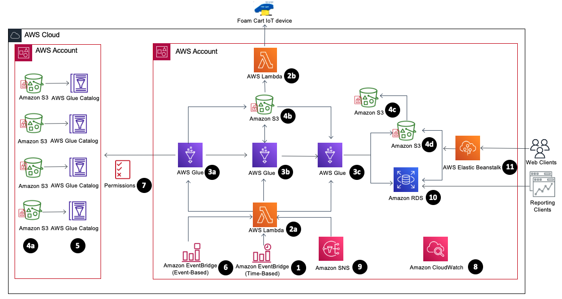
The following diagram illustrates the architecture of our wash analytics solution using AWS services.
The solution includes the following components:
EventBridge (1) – We use an EventBridge (time-based) to schedule the daily process to capture the delta changes between the runs.
Lambda (2a) – Lambda orchestrates the AWS Glue jobs initiation, backup, and recovery on failure for each stage, utilizing EventBridge (event-based) for the alerting of these events.
Lambda (2b) – Foam cart events from IoT devices are loaded into staging buckets in Amazon Simple Storage Service (Amazon S3) daily.
AWS Glue (3) – The wash analytics need to handle a small subset of data daily, but the initial historical load and transformation is huge. Because AWS Glue is serverless, it’s easy to set up and run with no maintenance.
Copy job (3a) – We use an AWS Glue copy job to copy only the required subset of data from across AWS accounts by connecting to AWS Glue Data Catalog tables using a cross-account AWS Identity and Access Management (IAM) role.
Business transformation jobs (3b, 3c) – When the copy job is complete, Lambda triggers subsequent AWS Glue jobs. Because our jobs are both compute and memory intensive, we use G2.x worker nodes. We can use Amazon CloudWatch metrics to fine-tune our jobs to use the right worker nodes. To handle complex calculations, we split large jobs up into multiple jobs by pipelining the output of one job as input to another job.
Source S3 buckets (4a) – Flights, wash events, and other engine parameter data is available in source buckets in a different AWS account exposed via Data Catalog tables.
Stage S3 bucket (4b) – Data from another AWS account is required for calculations, and all the intermediate outputs from the AWS Glue jobs are written to the staging bucket.
Backup S3 bucket (4c) – Every day before starting the AWS Glue job, the previous day’s output from the output bucket is backed up in the backup bucket. In case of any job failure, the data is recovered from this bucket.
Output S3 bucket (4d) – The final output from the AWS Glue jobs is written to the output bucket.
Continuing our analysis of the architecture components, we also use the following:
AWS Glue Data Catalog tables (5) – We catalog flights, wash events, and other engine parameter data using Data Catalog tables, which are accessed by AWS Glue copy jobs from another AWS account.
EventBridge (6) – We use EventBridge (event-based) to monitor for AWS Glue job state changes (SUCEEDED, FAILED, TIMEOUT, and STOPPED) and orchestrate the workflow, including backup, recovery, and job status notifications.
IAM role (7) – We set up cross-account IAM roles to copy the data from one account to another from the AWS Glue Data Catalog tables.
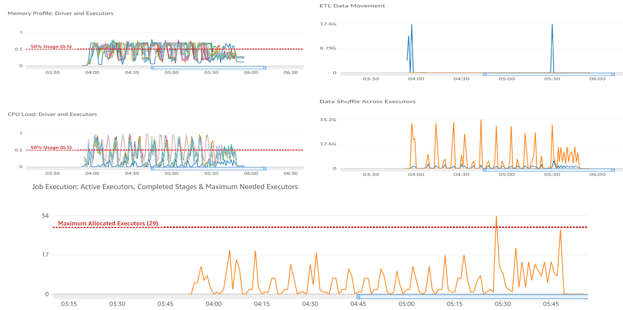
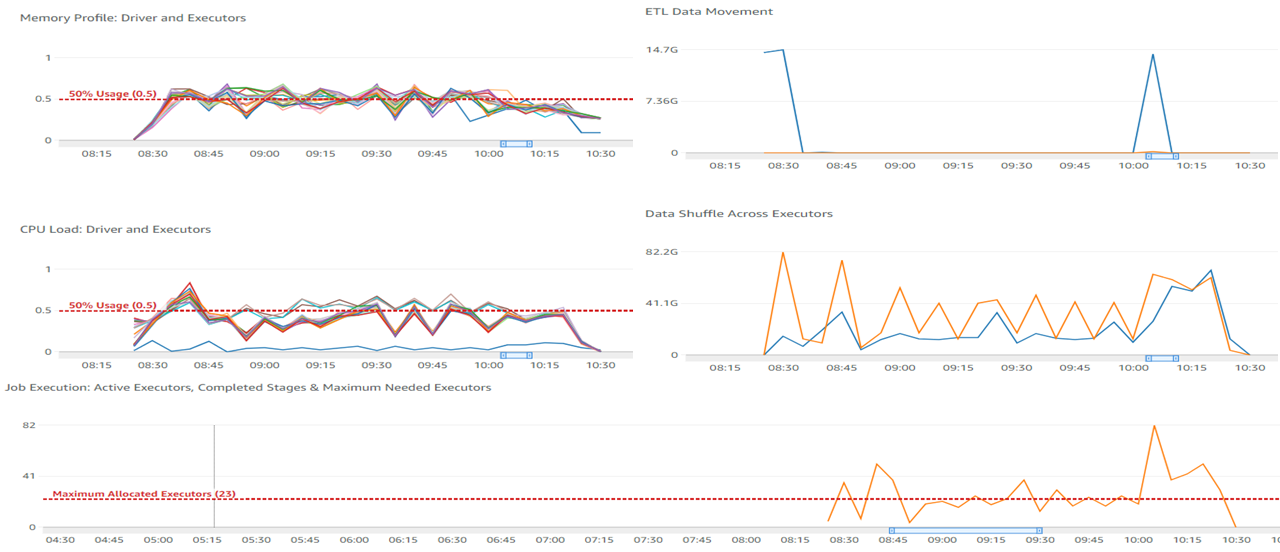
CloudWatch metrics (8) – You can monitor many different CloudWatch metrics. The following metrics can help you decide on horizontal or vertical scaling when fine-tuning the AWS Glue jobs:
CPU load of the driver and executors
Memory profile of the driver
ETL data movement
Data shuffle across executors
Job run metrics, including active executors, completed stages, and maximum needed executors
Amazon SNS (9) – Amazon Simple Notification Service (Amazon SNS) automatically sends notifications to the support group on the error status of jobs, so they can take corrective action upon failure.
Web application (11) – A web application is hosted on AWS Elastic Beanstalk, and is enabled with Auto Scaling exposed for clients to access the analytics data.
Implementation strategy
Implementing our solution included the following considerations:
Security – The data required for running analytics is present in different data sources and different AWS accounts. We needed to craft well-thought-out role-based access policies for accessing the data.
Selecting the right programming paradigm – PySpark does lazy evaluation while working with data frames. For PySpark to work efficiently with AWS Glue, we created data frames with required columns upfront and performed column-wise operations.
Choosing the right persistence storage – Writing to Amazon S3 enables multiple consumption patterns, and writes are much faster due to parallelism.
If we’re writing to Amazon RDS (for supporting legacy systems), we need to watch out for database connectivity and buffer lock issues while writing from AWS Glue jobs.
Data partitioning – Identifying the right key combination is important for partitioning the data for Spark to perform optimally. Our initial runs (without data partition) with 30 workers of type G2.x took 2 hours and 4 minutes to complete.
The following screenshot shows our CloudWatch metrics.
After a few dry runs, we were able to arrive at partitioning by a specific column (df.repartition(columnKey)) and with 24 workers of type G2.x, the job completed in 2 hours and 7 minutes. The following screenshot shows our new metrics.
We can observe a difference in CPU and memory utilization—running with even fewer nodes shows a smaller CPU utilization and memory footprint.
The following table shows how we achieved the final transformation with the strategies we discussed.
Iteration
Run Time
AWS Glue Job Status
Strategy
1
~12 hours
Unsuccessful/Stopped
Initial iteration
2
~9 hours
Unsuccessful/Stopped
Changing code to PySpark methodology
3
5 hours, 11 minutes
Partial success
Splitting a complex large job into multiple jobs
4
3 hours, 33 minutes
Success
Partitioning by column key
5
2 hours, 39 minutes
Success
Changing CSV to Parquet file format while storing the copied data from another AWS account and intermediate results in the stage S3 bucket
6
2 hours, 9 minutes
Success
Infra scaling: horizontal and vertical scaling
Conclusion
In this post, we saw how to build a cost-effective, maintenance-free solution using serverless AWS services to process large-scale data. We also learned how to gain optimal AWS Glue job performance with key partitioning, using the Parquet data format while persisting in Amazon S3, splitting complex jobs into multiple jobs, and using the right programming paradigm.
As we continue to solidify our data lake solution for data from various sources, we can use Amazon Redshift Spectrum to serve various future analytical use cases.
About the Authors
Giridhar G Jorapur is a Staff Infrastructure Architect at GE Aviation. In this role, he is responsible for designing enterprise applications, migration and modernization of applications to the cloud. Apart from work, Giri enjoys investing himself in spiritual wellness. Connect him on LinkedIn.
На 16 януари 2021 г. “Биволъ” съобщи, че назначената от служебния министър Виолета Комитова за изпълнителен директор на “Автомагистрали” ЕАД (АМ ЕАД) Десислава Христова е подписвала инхаусите за АМ “Хемус”…
Вицепремиерът и министър на регионалното развитие от квотата на „Има такъв народ“ Гроздан Караджов е назначил замесени в “инхаус” сделки за укрепване на свлачища и АМ “Хемус” в управителния съвет…
Many customers want to provision Amazon Web Services (AWS) cloud resources quickly and consistently with lifecycle management, by treating infrastructure as code (IaC). Commonly used services are AWS CloudFormation and HashiCorp Terraform. Currently, customers set up Amazon Connect data streaming manually, as the service is not available under CloudFormation resource types. Customers may want to extend it to retrieve real-time contact and agent data. Integration is done manually and can result in issues with IaC.
Amazon Connect contact trace records (CTRs) capture the events associated with a contact in the contact center. Amazon Connect agent event streams are Amazon Kinesis Data Streams that provide near real-time reporting of agent activity within the Amazon Connect instance. The events published to the stream include these contact control panel (CCP) events:
Agent login
Agent logout
Agent connects with a contact
Agent status change, such as to available to handle contacts, or on break, or at training.
In this blog post, we will show you how to automate Amazon Connect data streaming using AWS Cloud Development Kit (AWS CDK). AWS CDK is an open source software development framework to define your cloud application resources using familiar programming languages. We will create a custom CDK resource, which in turn uses Amazon Connect API. This can be used as a template to automate other parts of Amazon Connect, or for other AWS services that don’t expose its full functionality through CloudFormation.
Overview of Amazon Connect automation solution
Amazon Connect is an omnichannel cloud contact center that helps you provide superior customer service. We will stream Amazon Connect agent activity and contact trace records to Amazon Kinesis. We will assume that data will then be used by other services or third-party integrations for processing. Here are the high-level steps and AWS services that we are going use, see Figure 1:
Amazon Connect: We will create an instance and enable data streaming
Cloud Deployment Toolkit: We will create custom resource and orchestrate automation
Third-party tool or Amazon S3: Used as a destination of Connect data via Amazon Kinesis data
Figure 1. Connect data streaming automation workflow
Walkthrough and deployment tasks
Sample code for this solution is provided in this GitHub repo. The code is packaged as a CDK application, so the solution can be deployed in minutes. The deployment tasks are as follows:
Deploy the CDK app
Update Amazon Connect instance settings
Import the demo flow and data
Custom Resources enables you to write custom logic in your CloudFormation deployment. You implement the creation, update, and deletion logic to define the custom resource deployment.
CDK implements the AWSCustomResource, which is an AWS Lambda backed custom resource that uses the AWS SDK to provision your resources. This means that the CDK stack deploys a provisioning Lambda. Upon deployment, it calls the AWS SDK API operations that you defined for the resource lifecycle (create, update, and delete).
Prerequisites
For this walkthrough, you need the following prerequisites:
This post uses an AWS CDK stack written in Python; follow the instructions in the CDK Getting Started guide to set up your environment.
An Amazon Connect instance. If you do not have one, you can deploy a Connect instance and claim a phone number, see Set up your Amazon Connect instance.
Deploy and verify
1. Deploy the CDK application.
The resources required for this demo are packaged as a CDK app. Before proceeding, confirm you have command line interface (CLI) access to the AWS account where you would like to deploy your solution.
Open a terminal window and clone the GitHub repository in a directory of your choice: git clone [email protected]:aws-samples/connect-cdk-blog
Navigate to the cdk-app directory and follow the deployment instructions. The default Region is usually us-east-1. If you would like to deploy in another Region, you can run: export AWS_DEFAULT_REGION=eu-central-1
2. Create the CloudFormation stack by initiating the following commands.
Note: By default, the stack will create contact trace records stream [ctrStreamName] as a Kinesis Data Stream. If you want to use an Amazon Kinesis Data Firehose delivery stream instead, you can modify this behavior by going to cdk.json and adding “ctr_stream_type”: “KINESIS_FIREHOSE” as a parameter under “context.”
Once the status of CloudFormation stack is updated to CREATE_COMPLETE, the following resources are created:
Kinesis Data Stream
IAM roles
Lambda
3. Verify the integration.
Kinesis Data Streams are added to the Amazon Connect instance
Figure 2. Screenshot of Amazon Connect with Data Streaming enabled
Cleaning up
You can remove all resources provisioned for the CDK app by running the following command under connect-app directory:
cdk destroy
This will not remove your Amazon Connect instance. You can remove it by navigating to the AWS Management Console -> Services -> Amazon Connect. Find your Connect instance and click Delete.
Conclusion
In this blog, we demonstrated how to maintain Amazon Connect as Infrastructure as Code (IaC). Using a custom resource of AWS CDK, we have shown how to automate setting Amazon Kinesis Data Streams to Data Streaming in Amazon Connect. The same approach can be extended to automate setting other Amazon Connect properties such as Amazon Lex, AWS Lambda, Amazon Polly, and Customer Profiles. This approach will help you to integrate Amazon Connect with your Workflow Management Application in a faster and consistent manner, and reduce manual configuration.
Senators have reintroduced the EARN IT Act, requiring social media companies (among others) to administer a massive surveillance operation on their users:
A group of lawmakers led by Sen. Richard Blumenthal (D-CT) and Sen. Lindsey Graham (R-SC) have re-introduced the EARN IT Act, an incredibly unpopular bill from 2020 that was dropped in the face of overwhelming opposition. Let’s be clear: the new EARN IT Act would pave the way for a massive new surveillance system, run by private companies, that would roll back some of the most important privacy and security features in technology used by people around the globe. It’s a framework for private actors to scan every message sent online and report violations to law enforcement. And it might not stop there. The EARN IT Act could ensure that anything hosted online — backups, websites, cloud photos, and more — is scanned.
Version
1.20.0 of the
GStreamer multimedia system is out. Changes include a new high-level
playback library replacing GstPlayer, decoding support for WebM Alpha,
updated Rust bindings, and more; see the announcement for lots of details.
Loading a BPF program into the kernel involves a lot of steps, including
verification, permissions checking, linking to in-kernel helper functions,
and compilation to the native instruction format. Underneath all of that,
though, lies one other simple task: allocating some memory to store the
compiled BPF program in the kernel’s address space. It turns out that this
allocation
can be somewhat wasteful of memory in current kernels, especially on
systems where large numbers of BPF programs are loaded. This
patch set from Song Liu seeks to remedy this problem by introducing yet
another specialized memory allocator into the kernel.
Chances are you might have heard of io_uring. It first appeared in Linux 5.1, back in 2019, and was advertised as the new API for asynchronous I/O. Its goal was to be an alternative to the deemed-to-be-broken-beyond-repair AIO, the “old” asynchronous I/O API.
Calling io_uring just an asynchronous I/O API doesn’t do it justice, though. Underneath the API calls, io_uring is a full-blown runtime for processing I/O requests. One that spawns threads, sets up work queues, and dispatches requests for processing. All this happens “in the background” so that the user space process doesn’t have to, but can, block while waiting for its I/O requests to complete.
A runtime that spawns threads and manages the worker pool for the developer makes life easier, but using it in a project begs the questions:
1. How many threads will be created for my workload by default?
2. How can I monitor and control the thread pool size?
By default, io_uring limits the unbounded workers created to the maximum processor count set by RLIMIT_NPROC and the bounded workers is a function of the SQ ring size and the number of CPUs in the system.
… it also leads to more questions:
3. What is an unbounded worker?
4. How does it differ from a bounded worker?
Things seem a bit under-documented as is, hence this blog post. Hopefully, it will provide the clarity needed to put io_uring to work in your project when the time comes.
Before we dig in, a word of warning. This post is not meant to be an introduction to io_uring. The existing documentation does a much better job at showing you the ropes than I ever could. Please give it a read first, if you are not familiar yet with the io_uring API.
Not all I/O requests are created equal
io_uring can perform I/O on any kind of file descriptor; be it a regular file or a special file, like a socket. However, the kind of file descriptor that it operates on makes a difference when it comes to the size of the worker pool.
io-wq divides work into two categories: 1. Work that completes in a bounded time, like reading from a regular file or a block device. This type of work is limited based on the size of the SQ ring. 2. Work that may never complete, we call this unbounded work. The amount of workers here is limited by RLIMIT_NPROC.
This answers the latter two of our open questions. Unbounded workers handle I/O requests that operate on neither regular files (S_IFREG) nor block devices (S_ISBLK). This is the case for network I/O, where we work with sockets (S_IFSOCK), and other special files like character devices (e.g. /dev/null).
We now also know that there are different limits in place for how many bounded vs unbounded workers there can be running. So we have to pick one before we dig further.
Capping the unbounded worker pool size
Pushing data through sockets is Cloudflare’s bread and butter, so this is what we are going to base our test workload around. To put it in io_uring lingo – we will be submitting unbounded work requests.
While doing that, we will observe how io_uring goes about creating workers.
To observe how io_uring goes about creating workers we will ask it to read from a UDP socket multiple times. No packets will arrive on the socket, so we will have full control over when the requests complete.
$ ./target/debug/udp-read -h
udp-read 0.1.0
read from UDP socket with io_uring

USAGE:
    udp-read [FLAGS] [OPTIONS]

FLAGS:
    -a, --async      Set IOSQE_ASYNC flag on submitted SQEs
    -h, --help       Prints help information
    -V, --version    Prints version information

OPTIONS:
    -c, --cpu <cpu>...                     CPU to run on when invoking io_uring_enter for Nth ring (specify multiple
                                           times) [default: 0]
    -w, --workers <max-unbound-workers>    Maximum number of unbound workers per NUMA node (0 - default, that is
                                           RLIMIT_NPROC) [default: 0]
    -r, --rings <num-rings>                Number io_ring instances to create per thread [default: 1]
    -t, --threads <num-threads>            Number of threads creating io_uring instances [default: 1]
    -s, --sqes <sqes>                      Number of read requests to submit per io_uring (0 - fill the whole queue)
                                           [default: 0]
While it is parametrized for easy experimentation, at its core it doesn’t do much. We fill the submission queue with read requests from a UDP socket and then wait for them to complete. But because data doesn’t arrive on the socket out of nowhere, and there are no timeouts set up, nothing happens. As a bonus, we have complete control over when requests complete, which will come in handy later.
Let’s run the test workload to convince ourselves that things are working as expected. strace won’t be very helpful when using io_uring. We won’t be able to tie I/O requests to system calls. Instead, we will have to turn to in-kernel tracing.
Thankfully, io_uring comes with a set of ready to use static tracepoints, which save us the trouble of digging through the source code to decide where to hook up dynamic tracepoints, known as kprobes.
We can discover the tracepoints with perf list or bpftrace -l, or by browsing the events/ directory on the tracefs filesystem, usually mounted under /sys/kernel/tracing.
$ sudo perf list 'io_uring:*'

List of pre-defined events (to be used in -e):

  io_uring:io_uring_complete                         [Tracepoint event]
  io_uring:io_uring_cqring_wait                      [Tracepoint event]
  io_uring:io_uring_create                           [Tracepoint event]
  io_uring:io_uring_defer                            [Tracepoint event]
  io_uring:io_uring_fail_link                        [Tracepoint event]
  io_uring:io_uring_file_get                         [Tracepoint event]
  io_uring:io_uring_link                             [Tracepoint event]
  io_uring:io_uring_poll_arm                         [Tracepoint event]
  io_uring:io_uring_poll_wake                        [Tracepoint event]
  io_uring:io_uring_queue_async_work                 [Tracepoint event]
  io_uring:io_uring_register                         [Tracepoint event]
  io_uring:io_uring_submit_sqe                       [Tracepoint event]
  io_uring:io_uring_task_add                         [Tracepoint event]
  io_uring:io_uring_task_run                         [Tracepoint event]
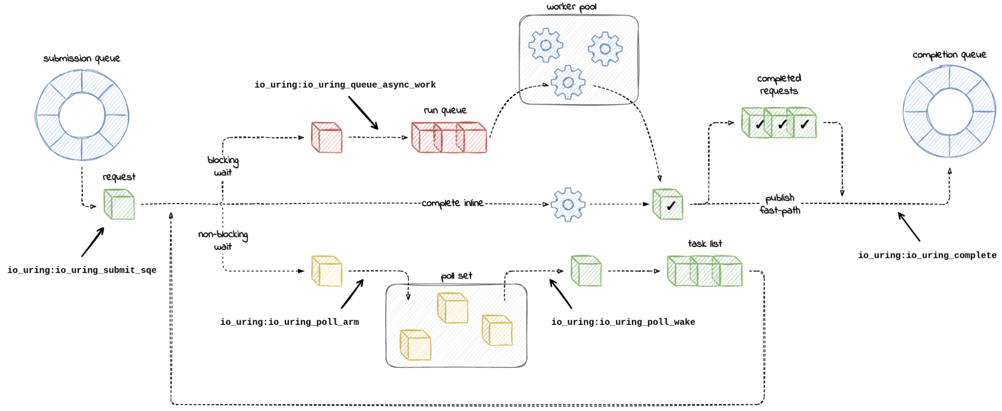
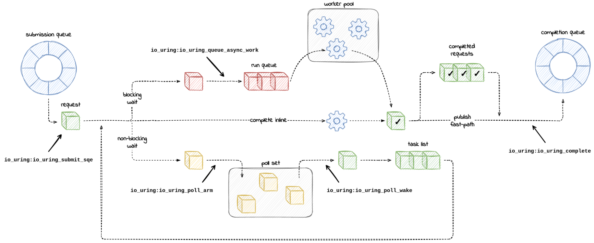
Judging by the number of tracepoints to choose from, io_uring takes visibility seriously. To help us get our bearings, here is a diagram that maps out paths an I/O request can take inside io_uring code annotated with tracepoint names – not all of them, just those which will be useful to us.
Starting on the left, we expect our toy workload to push entries onto the submission queue. When we publish submitted entries by calling io_uring_enter(), the kernel consumes the submission queue and constructs internal request objects. A side effect we can observe is a hit on the io_uring:io_uring_submit_sqe tracepoint.
$ sudo perf stat -e io_uring:io_uring_submit_sqe -- timeout 1 ./udp-read

 Performance counter stats for 'timeout 1 ./udp-read':

              4096      io_uring:io_uring_submit_sqe

       1.049016083 seconds time elapsed

       0.003747000 seconds user
       0.013720000 seconds sys
But, as it turns out, submitting entries is not enough to make io_uring spawn worker threads. Our process remains single-threaded:
So, by default, io_uring performs a non-blocking read on sockets. This is bound to fail with -EAGAIN in our case. What follows is that io_uring registers a wake-up call (io_async_wake()) for when the socket becomes readable. There is no need to perform a blocking read, when we can wait to be notified.
This resembles polling the socket with select() or [e]poll() from user space. There is no timeout, if we didn’t ask for it explicitly by submitting an IORING_OP_LINK_TIMEOUT request. io_uring will simply wait indefinitely.
We can observe io_uring when it calls vfs_poll, the machinery behind non-blocking I/O, to monitor the sockets. If that happens, we will be hitting the io_uring:io_uring_poll_arm tracepoint. Meanwhile, the wake-ups that follow, if the polled file becomes ready for I/O, can be recorded with the io_uring:io_uring_poll_wake tracepoint embedded in io_async_wake() wake-up call.
This is what we are experiencing. io_uring is polling the socket for read-readiness:
To make io_uring spawn worker threads, we have to force the read requests to be processed concurrently in a blocking fashion. We can do this by marking the I/O requests as asynchronous. As io_uring_enter(2) man-page says:
  IOSQE_ASYNC
         Normal operation for io_uring is to try and  issue  an
         sqe  as non-blocking first, and if that fails, execute
         it in an async manner. To support more efficient over‐
         lapped  operation  of  requests  that  the application
         knows/assumes will always (or most of the time) block,
         the  application can ask for an sqe to be issued async
         from the start. Available since 5.6.
The thread count went up by the number of submitted I/O requests (4,096). And there is one extra thread – the main thread. io_uring has spawned workers.
If we trace it again, we see that requests are now taking the blocking-read path, and we are hitting the io_uring:io_uring_queue_async_work tracepoint on the way.
$ sudo perf stat -a -e io_uring:io_uring_poll_arm,io_uring:io_uring_queue_async_work -- ./udp-read --async
^C./udp-read: Interrupt

 Performance counter stats for 'system wide':

                 0      io_uring:io_uring_poll_arm
              4096      io_uring:io_uring_queue_async_work

       1.335559294 seconds time elapsed

$
We got what we wanted. We are now using the worker thread pool.
However, having 4,096 threads just for reading one socket sounds like overkill. If we were to limit the number of worker threads, how would we go about that? There are four ways I know of.
Method 1 – Limit the number of in-flight requests
If we take care to never have more than some number of in-flight blocking I/O requests, then we will have more or less the same number of workers. This is because:
io_uring spawns workers only when there is work to process. We control how many requests we submit and can throttle new submissions based on completion notifications.
io_uring retires workers when there is no more pending work in the queue. Although, there is a grace period before a worker dies.
The downside of this approach is that by throttling submissions, we reduce batching. We will have to drain the completion queue, refill the submission queue, and switch context with io_uring_enter() syscall more often.
We can convince ourselves that this method works by tweaking the number of submitted requests, and observing the thread count as the requests complete. The --sqes <n> option (submission queue entries) controls how many read requests get queued by our workload. If we want a request to complete, we simply need to send a packet toward the UDP socket we are reading from. The workload does not refill the submission queue.
In 5.15 the io_uring_register() syscall gained a new command for setting the maximum number of bound and unbound workers.
  IORING_REGISTER_IOWQ_MAX_WORKERS
         By default, io_uring limits the unbounded workers cre‐
         ated   to   the   maximum   processor   count  set  by
         RLIMIT_NPROC and the bounded workers is a function  of
         the SQ ring size and the number of CPUs in the system.
         Sometimes this can be excessive (or  too  little,  for
         bounded),  and  this  command provides a way to change
         the count per ring (per NUMA node) instead.

         arg must be set to an unsigned int pointer to an array
         of  two values, with the values in the array being set
         to the maximum count of workers per NUMA node. Index 0
         holds  the bounded worker count, and index 1 holds the
         unbounded worker  count.  On  successful  return,  the
         passed  in array will contain the previous maximum va‐
         lyes for each type. If the count being passed in is 0,
         then  this  command returns the current maximum values
         and doesn't modify the current setting.  nr_args  must
         be set to 2, as the command takes two values.

         Available since 5.15.
By the way, if you would like to grep through the io_uring man pages, they live in the liburing repo maintained by Jens Axboe – not the go-to repo for Linux API man-pages maintained by Michael Kerrisk.
Since it is a fresh addition to the io_uring API, the io-uring Rust library we are using has not caught up yet. But with a bit of patching, we can make it work.
We can tell our toy program to set IORING_REGISTER_IOWQ_MAX_WORKERS (= 19 = 0x13) by running it with the --workers <N> option:
This works perfectly. We have spawned just eight io_uring worker threads to handle 4k of submitted read requests.
Question remains – is the set limit per io_uring instance? Per thread? Per process? Per UID? Read on to find out.
Method 3 – Set RLIMIT_NPROC resource limit
A resource limit for the maximum number of new processes is another way to cap the worker pool size. The documentation for the IORING_REGISTER_IOWQ_MAX_WORKERS command mentions this.
This resource limit overrides the IORING_REGISTER_IOWQ_MAX_WORKERS setting, which makes sense because bumping RLIMIT_NPROC above the configured hard maximum requires CAP_SYS_RESOURCE capability.
Setting the new process limit without using a dedicated UID or outside a dedicated user namespace, where other processes are running under the same UID, can have surprising effects.
Why? io_uring will try over and over again to scale up the worker pool, only to generate a bunch of -EAGAIN errors from create_io_worker() if it can’t reach the configured RLIMIT_NPROC limit:
We are hogging one core trying to spawn new workers. This is not the best use of CPU time.
So, if you want to use RLIMIT_NPROC as a safety cap over the IORING_REGISTER_IOWQ_MAX_WORKERS limit, you better use a “fresh” UID or a throw-away user namespace:
Anti-Method 4 – cgroup process limit – pids.max file
There is also one other way to cap the worker pool size – limit the number of tasks (that is, processes and their threads) in a control group.
It is an anti-example and a potential misconfiguration to watch out for, because just like with RLIMIT_NPROC, we can fall into the same trap where io_uring will burn CPU:
Here, we again see io_uring wasting time trying to spawn more workers without success. The kernel does not let the number of tasks within the service’s control group go over the limit.
Okay, so we know what is the best and the worst way to put a limit on the number of io_uring workers. But is the limit per io_uring instance? Per user? Or something else?
One ring, two ring, three ring, four …
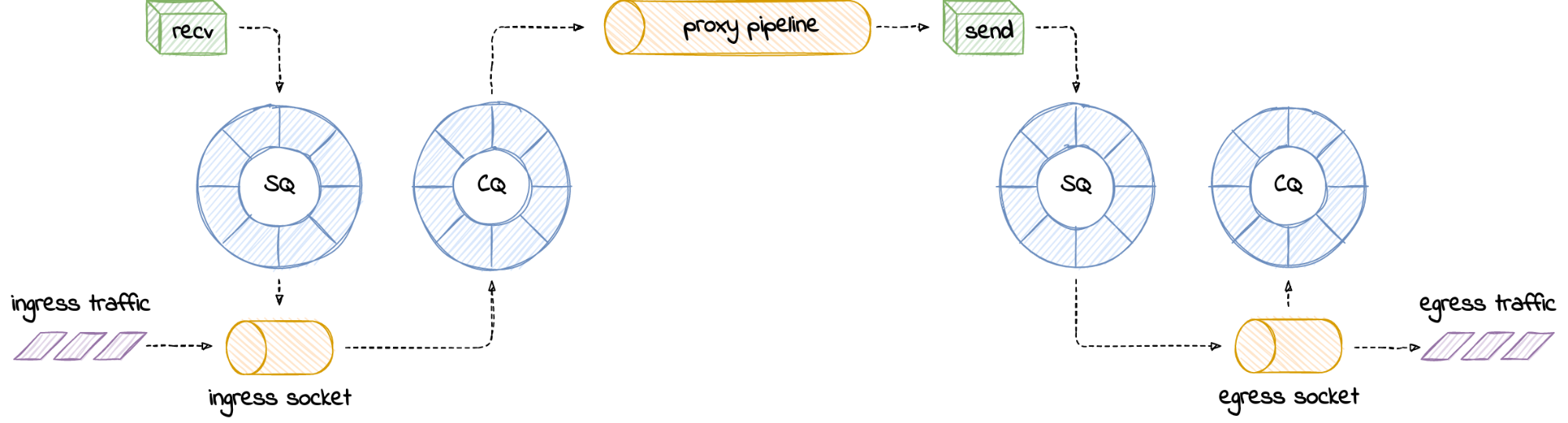
Your process is not limited to one instance of io_uring, naturally. In the case of a network proxy, where we push data from one socket to another, we could have one instance of io_uring servicing each half of the proxy.
How many worker threads will be created in the presence of multiple io_urings? That depends on whether your program is single- or multithreaded.
In the single-threaded case, if the main thread creates two io_urings, and configures each io_uring to have a maximum of two unbound workers, then:
… four workers will be spawned in total – two for each of the program threads. This is reflected by the owner thread ID present in the worker’s name (iou-wrk-<tid>).
So you might think – “It makes sense! Each thread has their own dedicated pool of I/O workers, which service all the io_uring instances operated by that thread.”
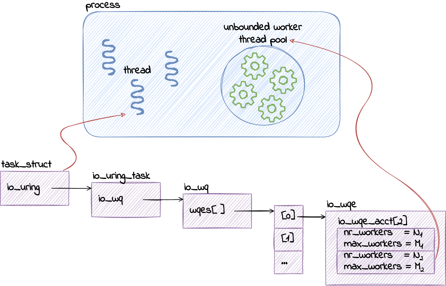
And you would be right1. If we follow the code – task_struct has an instance of io_uring_task, aka io_uring context for the task2. Inside the context, we have a reference to the io_uring work queue (struct io_wq), which is actually an array of work queue entries (struct io_wqe). More on why that is an array soon.
Moving down to the work queue entry, we arrive at the work queue accounting table (struct io_wqe_acct [2]), with one record for each type of work – bounded and unbounded. This is where io_uring keeps track of the worker pool limit (max_workers) the number of existing workers (nr_workers).
The perhaps not-so-obvious consequence of this arrangement is that setting just the RLIMIT_NPROC limit, without touching IORING_REGISTER_IOWQ_MAX_WORKERS, can backfire for multi-threaded programs.
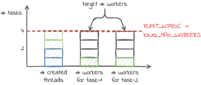
See, when the maximum number of workers for an io_uring instance is not configured, it defaults to RLIMIT_NPROC. This means that io_uring will try to scale the unbounded worker pool to RLIMIT_NPROC for each thread that operates on an io_uring instance.
A multi-threaded process, by definition, creates threads. Now recall that the process management in the kernel tracks the number of tasks per UID within the user namespace. Each spawned thread depletes the quota set by RLIMIT_NPROC. As a consequence, io_uring will never be able to fully scale up the worker pool, and will burn the CPU trying to do so.
Lastly, there’s the case of NUMA systems with more than one memory node. io_uring documentation clearly says that IORING_REGISTER_IOWQ_MAX_WORKERS configures the maximum number of workers per NUMA node.
That is why, as we have seen, io_wq.wqes is an array. It contains one entry, struct io_wqe, for each NUMA node. If your servers are NUMA systems like Cloudflare, that is something to take into account.
Luckily, we don’t need a NUMA machine to experiment. QEMU happily emulates NUMA architectures. If you are hardcore enough, you can configure the NUMA layout with the right combination of -smp and -numa options.
But why bother when the libvirt provider for Vagrant makes it so simple to configure a 2 node / 4 CPU layout:
… we get just two workers on a machine with two NUMA nodes. Not the outcome we were hoping for.
Why are we not reaching the expected pool size of <max workers> × <# NUMA nodes> = 2 × 2 = 4 workers? And is it possible to make it happen?
Reading the code reveals that – yes, it is possible. However, for the per-node worker pool to be scaled up for a given NUMA node, we have to submit requests, that is, call io_uring_enter(), from a CPU that belongs to that node. In other words, the process scheduler and thread CPU affinity have a say in how many I/O workers will be created.
We can demonstrate the effect that jumping between CPUs and NUMA nodes has on the worker pool by operating two instances of io_uring. We already know that having more than one io_uring instance per thread does not impact the worker pool limit.
This time, however, we are going to ask the workload to pin itself to a particular CPU before submitting requests with the --cpu option – first it will run on CPU 0 to enter the first ring, then on CPU 2 to enter the second ring.
Voilà. We have reached the said limit of <max workers> x <# NUMA nodes>.
Outro
That is all for the very first installment of the Missing Manuals. io_uring has more secrets that deserve a write-up, like request ordering or handling of interrupted syscalls, so Missing Manuals might return soon.
In the meantime, please tell us what topic would you nominate to have a Missing Manual written?
Oh, and did I mention that if you enjoy putting cutting edge Linux APIs to use, we are hiring? Now also remotely 🌎.
_____
1And it probably does not make the users of runtimes that implement a hybrid threading model, like Golang, too happy. 2To the Linux kernel, processes and threads are just kinds of tasks, which either share or don’t share some resources.
Version 15 of the
venerable Slackware distribution has been released.
The challenge this time around was to adopt as much of the good
stuff out there as we could without changing the character of the
operating system. Keep it familiar, but make it modern. And boy
did we have our work cut out for us. We adopted PAM (finally) as
projects we needed dropped support for pure shadow passwords. We
switched from ConsoleKit2 to elogind, making it much easier to
support software that targets that Other Init System and bringing
us up-to-date with the XDG standards. We added support for PipeWire
as an alternate to PulseAudio, and for Wayland sessions in addition
to X11.
A bit more information can be found in the release
notes. Many of us got our start with Slackware; it is good to see that
it’s still out there and true to form.
For this installment of 7Rapid Questions, we sat down with Soumi Mukherjee, APAC Sales Manager – ANZ North Sales, to learn more about what drives her in her role at Rapid7.
1. Why did you join Rapid7?
The truth is I joined for the people. I worked for a Rapid7 channel partner prior, and my interaction with the Rapid7 team back then gave me an impression of a company built on a culture of respect, trust, and high standards. I wanted to be a part of it!
2. Describe what your teams do in a few words?
We help customers achieve their cybersecurity goals by connecting them to the right products and solutions.
3. What can a candidate do to stand out in the interview process?
Be authentic, and bring your real self! If you’re asked to do a presentation round and you do your best pitch by whiteboarding and not slides, do what is best for you!
4. Which of our core values do you embody the most?
I am an obsessive learner, and I feel the spirit of “Never Done” speaks to me naturally. The cybersecurity landscape is constantly changing, so it’s important to continue learning and anticipating what’s next.
5. What is it that makes cybersecurity such an exciting field?
No boring day, in a nutshell! The evolving threat landscape means, to stay relevant, we have to keep innovating and improving. This aspect keeps me excited.
6. What three words would you use to describe the culture at Rapid7?
Accountability, collaboration, empathy.
7. What’s the best team activity you’ve done?
I miss the in-person team events and can’t wait to get back to them when we can. One of my favorites was a barista course. Our team even competed to see who could make the best latte art! It was an amazing event, and I even have a certificate!
Want to join Soumi and her team? We’re hiring! Browse our open roles at Rapid7 here.
To provide the best experiences, we use technologies like cookies to store and/or access device information. Consenting to these technologies will allow us to process data such as browsing behavior or unique IDs on this site. Not consenting or withdrawing consent, may adversely affect certain features and functions.
Functional
Always active
The technical storage or access is strictly necessary for the legitimate purpose of enabling the use of a specific service explicitly requested by the subscriber or user, or for the sole purpose of carrying out the transmission of a communication over an electronic communications network.
Preferences
The technical storage or access is necessary for the legitimate purpose of storing preferences that are not requested by the subscriber or user.
Statistics
The technical storage or access that is used exclusively for statistical purposes.The technical storage or access that is used exclusively for anonymous statistical purposes. Without a subpoena, voluntary compliance on the part of your Internet Service Provider, or additional records from a third party, information stored or retrieved for this purpose alone cannot usually be used to identify you.
Marketing
The technical storage or access is required to create user profiles to send advertising, or to track the user on a website or across several websites for similar marketing purposes.