A Tale of Two Flink Autoscalers

Post Syndicated from Netflix Technology Blog original https://netflixtechblog.com/a-tale-of-two-flink-autoscalers-e9f6a1b1492b

Samuel Yeboah, Francesco Di Chiara and Mingliang Liu

Today, Netflix runs two Flink autoscalers. That is exactly one more than we want. We built the first one in-house years ago, when there was no mature option suited to our platform. The second came from the Apache Flink community, and it can scale workloads our homegrown system was never designed for. We now run both in production and are steadily converging on the open-source one. Along the way we learned some hard lessons about metrics, cost, and the real price of maintaining infrastructure you could instead adopt, and we hope they are useful whether you run a handful of Flink jobs or tens of thousands.

Why autoscaling is not optional at our scale

Netflix has run stream processing on Apache Flink since 2017. As of 2026 we operate more than 30,000 Flink jobs across multiple AWS regions. Most are not deployed by hand; they are generated by our managed platform Data Mesh, so the majority of users never touch a Flink job directly. A smaller but growing set are custom jobs, built and operated by teams across the company for use cases like personalization, Ads, and Live events. They range from single-operator jobs that shuttle records between Kafka topics to stateful pipelines with branches, joins, and terabytes of state, and their load swings with daily cycles, launches, and regional failovers.

Provisioning every one of those jobs for its peak is wasteful; provisioning for the average causes lag during surges. And in our platform a scaling action is not free: by default it means taking a savepoint, stopping the job gracefully, and restarting it at the new size, which for a large stateful job can take minutes. That leaves a genuinely hard question: how do you give each job the resources it needs, when it needs them, without a human in the loop and without breaking anything?

The first autoscaler: watching from outside

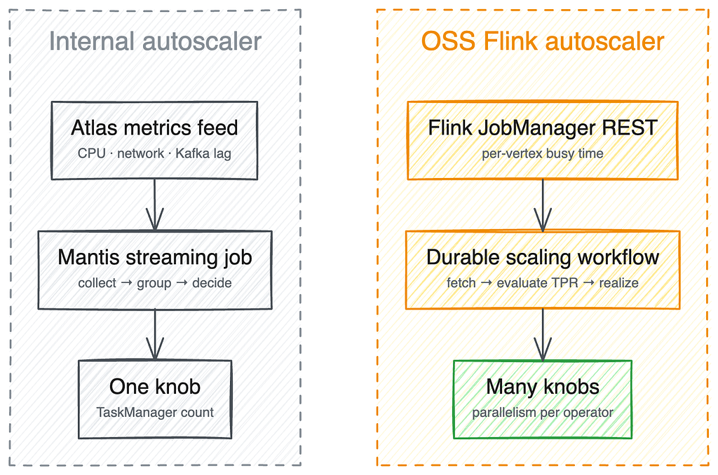
Our first answer, built around 2019, was an autoscaler shaped like a stream-processing job. It ran on Mantis, consuming a live feed of cluster-level metrics from Atlas, our telemetry platform including CPU, network, Kafka lag, input-rate, and consume-rate signals for every job. The scaler combined lag-derived catch-up time, CPU/network utilization thresholds, observed performance history, and regression over recent input rate to decide when to scale up or whether a smaller cluster could handle the lookahead window. Because the autoscaler operates independently of the Flink platform, it remains unaffected by issues within Flink itself. Building it as a streaming job also made it easy to scale. Each autoscaler node handled the metrics for a subset of Flink jobs, and we never had to write custom sharding or coordination logic to keep up with a growing Flink fleet. It reliably cut resource usage by 25–45% across thousands of managed pipelines. Check our previous talk at Flink Forward 2020.

But watching from outside has a ceiling. The system reasoned about a whole cluster through coarse container metrics, and it scaled a single knob, the total TaskManager count, so every operator in a job moved together. That fit the simple, single-operator pipelines it was built for, but not the multi-operator, stateful DAGs that teams were increasingly bringing to us for Ads, recommendations, and games. Those were exactly the jobs it could not reason about, and supporting each new case meant more custom logic rather than any general capability.

The autoscaler is only as good as the metrics served by external systems beneath it. Those metrics could miss real trouble: a job could be completely busy without any of it showing up as CPU utilization, leaving the job stuck in a degraded state the scaler had no way to see. Recently a networking migration quietly changed how some traffic was reported, and a subset of the Atlas metrics the scaler relied on stopped capturing everything accurately. The gap stayed invisible until it surfaced in production much later.

It was time to reconsider build versus buy.

The second autoscaler: reasoning from inside

When we started, the Flink community had no mature autoscaler to offer. By the time we re-evaluated, it did: the Apache Flink Autoscaler. Instead of watching containers from outside, it reasons from inside the job.

Figure 1: Architecture of the two Flink autoscalers

Its key idea is to estimate each operator’s true processing rate (TPR): the throughput it could sustain if it were fully busy. Flink reports, per subtask, the fraction of each second spent doing actual work, separate from time spent backpressured or idle. Dividing observed throughput by that busy fraction extrapolates capacity to full utilization: an operator handling 700 records/sec while busy 70% of the time has a TPR of 700 / 0.7 = 1,000 records/sec. Starting from the sources, the autoscaler walks the job graph and uses each operator’s TPR, its input/output ratios, and a target utilization to compute the parallelism every vertex needs so that no operator becomes the bottleneck, rather than resizing the whole cluster as a unit.

Figure 2: Flink job DAG: current → desired parallelism per vertex, based on busyness

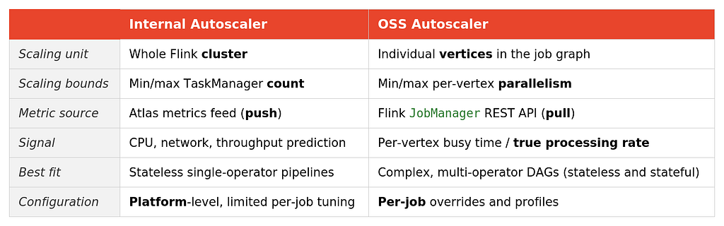
The two approaches make a different contract, summarized below.

Table 1: Comparison of the two Flink autoscalers

The decisive difference for us is the last two rows: the OSS autoscaler can scale exactly the stateful, multi-operator jobs our homegrown system could not, and it lets each job carry its own configuration — stabilization periods, thresholds, and other scaling behavior tuned to the workload.. That made it the natural fit for the custom jobs teams had been scaling by hand.

Making it work at Netflix scale

Adopting the algorithm was straightforward; the community had done the hard part. The work for us was running it reliably across our own jobs, and this is where our system differs most from the stock open-source deployment.

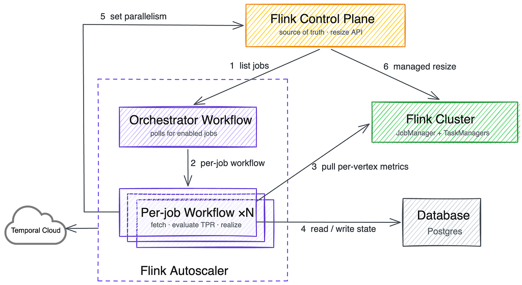
Firstly, the OSS autoscaler was originally architected to reside within the Kubernetes Operator for Flink, but our Flink platform runs on its own control plane, not that operator (see our previous talk at Current Conference 2024). Community later made a fantastic decision to keep the core logic as a standalone library. They refactored four generic interfaces that made it easy to plug directly into our internal ecosystem: a context carrying job metadata and REST API info, a state store, an event handler, and a realizer that applies scaling decisions.

That service is a Spring Boot application whose orchestration runs on Temporal, the durable workflow engine. An orchestrator workflow polls our Flink control plane about once a minute for the jobs with autoscaling enabled, and starts one long-running workflow per job. Each per-job workflow pulls that job’s per-vertex metrics from its Flink JobManager, runs the OSS evaluation algorithm, and, when a scaling decision results, hands it to a realizer that actuates the change through our Flink control plane.

Figure 3: The OSS-based Flink Autoscaler architecture with Temporal workflows

The workflow-per-job design was a direct response to pain. We first ran evaluations in a single batch loop over the whole set of jobs, and it was fragile: one slow or misbehaving job could stall metric collection and scaling for every job behind it. Giving each job its own durable workflow isolated that blast radius, so a single problematic job now fails and retries on its own, and the runtime scales out as we onboard more jobs.

Secondly, three engineering gaps stood between “works in community” and “works at Netflix scale”:

  • Metric collection at high parallelism. On big jobs, pulling metrics from the JobManager became a bottleneck, and part of the cause was in Flink’s runtime. To address that, we changed the JobManager to cache transient metric names and clean them up once instead of rescanning on every fetch, and we added server-side filtering so the autoscaler asks only for the metrics it needs. This let the autoscaler work on jobs up to 3,000 Flink subtasks, where it had previously struggled above roughly 1,000. Those are in our internal fork of Flink release, while some are contributed upstream such as FLINK-36172.
  • Preserving forward chaining. Two separate vertices joined by a forward connection must run at the same parallelism, because records are handed over in memory on a fixed local channel. Scale one of them alone and Flink does not fail; it silently converts that edge into a network shuffle. Our fork detects forward-connected subgraphs and scales each as a unit.
  • Respecting sink limits. Some sinks have finite write capacity, so we added detection for async-sink backpressure (also a fork change) to keep the autoscaler from scaling a job up into a sink that cannot absorb more.

Before it actuates anything, the realizer runs a set of safety checks. For example, it refuses to scale a job down in a region being evacuated during a company-wide region failover. It also verifies there is enough disk for the new cluster to hold the job’s checkpoint state, and it adds a small standby buffer for larger clusters.

The road to one autoscaler

Last year, the OSS-based autoscaler achieved general availability for custom jobs at Netflix, yielding promising initial outcomes. For instance, our client telemetry and logging team achieved a 58% reduction in its annualized Flink compute expenditures, saving approximately $1.1 million annually. This efficiency is driven by three key factors. First, whereas static provisioning must always account for peak loads, autoscaling dynamically adapts to daily cycles, capturing the drop in traffic during nights and weekends compared to weekday peaks. Second, rather than relying on teams to manually optimize resources following performance improvements or post-holiday slowdowns, the autoscaler continually adjusts capacity. Finally, adopting uniform container dimensions enables superior bin-packing and more granular scaling increments.

Additionally, scaling down too eagerly is its own trap. Cut too deep and CPU saturates, lag spikes, and the system cannot react instantly because its metric window and stabilization period have to rebuild after each restart. We now run a target utilization of 0.45, below the community default of 0.7, deliberately trading a little efficiency for stability. Fewer and calmer rescales are worth the marginal cost for large stateful jobs.

While our scaler provides fine-grained signals and vertex-level decision units for stateful DAGs, fast rescaling still heavily depends on Flink Core’s state restoration performance. Today, the biggest remaining cost in scaling a stateful job isn’t the scaler’s logic — it’s the restart and state recovery process itself. Flink 2 addresses this through its disaggregated state architecture, keeping state in external storage rather than on local disk, which can sharply reduce how much a rescale or recovery depends on total state size. Having started supporting Flink 2.2 at Netflix, we plan on experimenting with this new state backend to see if it can help eliminate state recovery bottlenecks when scaling large stateful jobs.

Looking ahead, we aim to migrate all internal scaler use cases onto the new one based on OSS autoscaler to simplify our operational surface area.

Key Takeaways

Along the way, three lessons that generalize beyond Flink:

  • Metric choice matters more than algorithm sophistication. Our most useful debugging was rarely about the scaling math; it was about which signal to trust most. Understand your metrics before you tune your algorithm.
  • Set sensible defaults, but leave room to tune. Our managed jobs are similar enough that one good default covers most of them untouched, which is the point of a platform. But forcing a single configuration on every job punishes the ones that do not fit, so we pair defaults with per-job overrides and deliberately hide the knobs that need deep expertise. Most teams should never have to think about the autoscaler.
  • Adopt, then extend. We built in-house because in 2019 nothing mature fit our platform. When a strong community project appeared, the right move was neither to defend our investment forever nor to rip it out overnight, but to adopt it for new workloads, contribute fixes back, and plan a deliberate migration.

Thanks to the Flink and Data Mesh teams for the control-plane changes this work depended on, to the Temporal team and our early pilot teams, and to the Apache Flink autoscaler maintainers whose foundation we built on. Special thanks to Andy Zhang, Calvin Cheung, Daniel Trager, Guil Pires, Mark Cho, Matthew Kornitsky, Nikhil Sulegaon, Sujay Jain, and Tom Lee.


A Tale of Two Flink Autoscalers was originally published in Netflix TechBlog on Medium, where people are continuing the conversation by highlighting and responding to this story.

Билбордовете извън градовете на България

Post Syndicated from Боян Юруков original https://yurukov.net/blog/2026/bulgariaads/

Всички забелязваме колко много реклама – най-вече такава на хазарт – има по улиците и пътищата на страната, по билбордове, фасади, покриви и какво ли не. Наскоро реших да науча повече как се получава така. Разгледах първо положението в София и създадох инструмент, с който всеки може да провери какви разрешения за реклама има около него и да подаде сигнал, ако вижда нередности. Аналогичен проблем има във всички български градове, но там липсват документи и данни, които да позволят такава прозрачност.

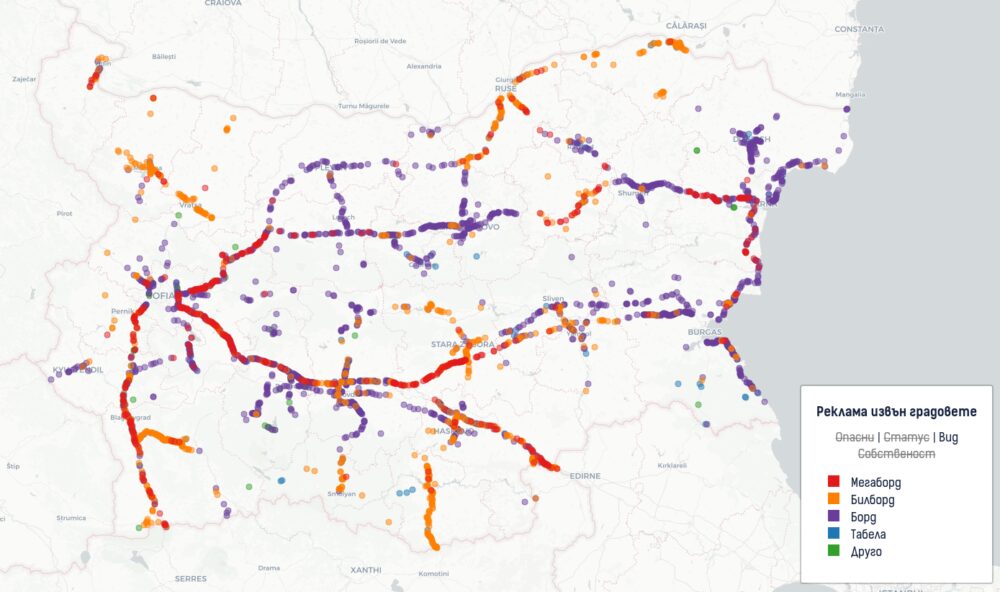
Обърнах се към билбордовете извън населените места на България, защото там виждаме преобладаващо реклама на хазарт и пренасищане. Както и преди, направих карта, която показва различни аспекти на проблема. Ще опиша методологията и какво показва по-късно. Ще започнем с проблемите, за които научих.

Практически всички са незаконни

Билбордовете извън населените места, а в някои случаи и в тях, следва да отговарят на Наредбата за специално използване на пътищата. Чл. 13 на тази наредба описва как се изграждат и пускат в експлоатация тези съоръжения. На практика фирмите плащат такса и минават многостъпков процес на одобрение при Агенция пътна инфраструктура. Няма значение дали билбордът ще е на частна, общинска или държавна земя – АПИ трябва да одобри и прибере такса, тъй като е край пътя. Същото се отнася впрочем и за бензиностанциите и крайпътните заведения.

Тук се сблъскваме с първото масово нарушение. Чл. 56 на Законът за устройството на територията позволява да се слагат такива преместваеми обекти, но ясно посочва, че разрешение за това може да се дава единствено от общината. Наредбата, по която оперира АПИ, сама споменава ЗУТ, не може да отмени закон и не дава право на АПИ да издава разрешителни за строеж. Всеки един от тези междуградски билбордове освен разрешение за специално ползване от АПИ следва да има и разрешение за поставяне от съответната община по проект.

Не открих нито едно разрешение за поставяне на билбордовете в данните на АПИ. Най-лесно беше да се провери в София, където Столична община отговаря за издаването на такива в началото на магистралите. В други общини беше значително по-трудно като повечето въобще не публикуват тези документи. Всички са задължени да ги качват в публичния регистър по ЗУТ. Наредба по него беше пусната най-накрая за обществено обсъждане от служебния кабинет на Гюров и от месеци чака един подпис от министър Шишков. Този регистър ще позволи лесно да се провери законността на всички тези и много други обекти и строежи. Именно това е и причината да беше бавен с години и да се отлага отново и при кабинета на Радев.

Вторият проблем са търговете. Не може да се използва държавна или общинска земя без да е проведен търг. Пътищата на страната са на държавна земя, а мнозинството от билбордовете са в същите имоти или на съседни общински. АПИ не е собственик на тази земя и няма право да я отдава. Това следва да прави областните управители или в случая на общинската земя – търгове към общината. Не открих в публичната информация за търгове нещо свързано с тези билбордове.

Състояние и обезопасяване

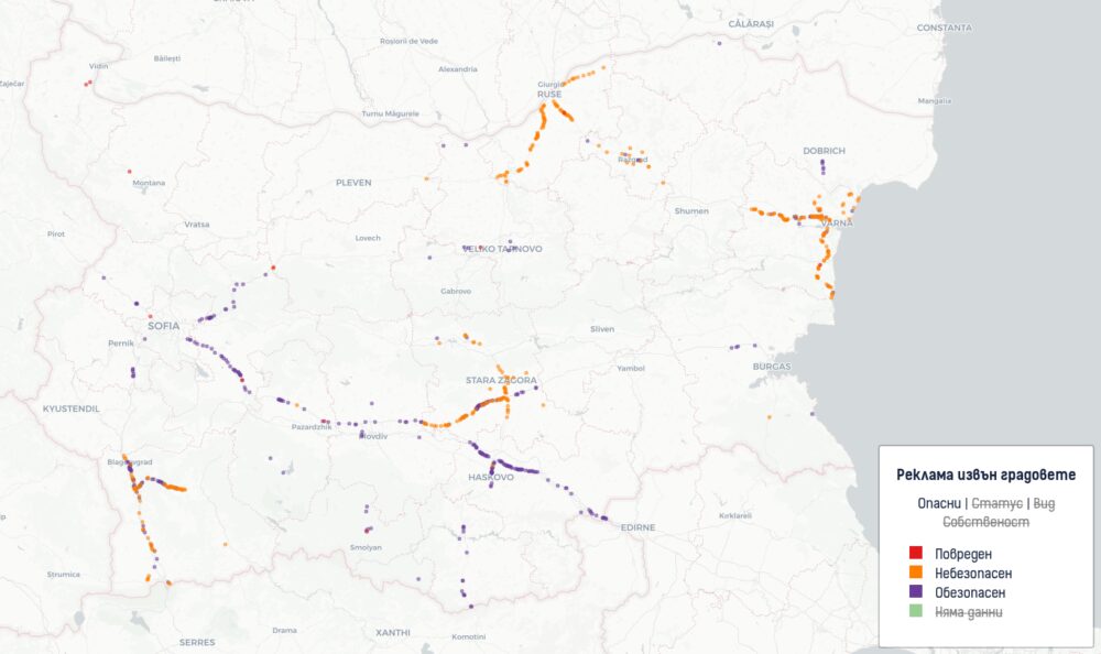
В данните на АПИ открих информация за местоположението и състоянието на 3783 билборда. Към средата на август 11 от тях са повредени. 369 или почти 10% са опасни, но необезопасени. Още 367 са обезопасени. Необезопасените са предимно около Стара Загора, Русе, Благоевград и Варна. Отговорност за това би следвало да е на собствениците и АПИ, а не на общините, които както описах по-горе изглежда не са включени в процеса.

102 или 2.6% са с изтекло или прекратено разрешение от АПИ. При 55 или 1.5% са намерени несъответствия с наредбата като недостатъчно отстояние от възли, пътя или един от друг. Към средата на август във фаза на проектиране са били 23 нови билборда.

12% от рекламите са мегабордове – онези най-големите на високи пилони. 27% са големи билбордове. 56% са малки билбордове, а останалото са табели и други видове реклама.

Ключовата 2027-ма

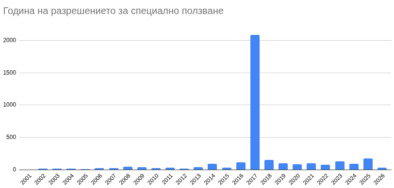
Чл. 16, ал. 4 от НСПП определя, че срокът за разрешението за специално ползване е 10 г. Това е различно от разрешение за строеж или поставяне, срокът на които се различава. В София, например, е 5 г. В данните на АПИ има дати на такова разрешение за 3600 обекта. Тук виждате разпределението им по години.

От тях е видно, че огромна част са издадени 2017 г. Всъщност, 61% от разрешенията за всички билбордове извън градовете изтичат до края на 2027 г. Интересното е, че още 12.5% са по-стари и би следвало вече да са изтекли. Само 20% тях обаче са отбелязани като такива. Това значи, че вероятно договорите им са подновени без да е отразено изрично в данните.

Това прави 2027-ма особено важна, защото позволява сериозно намаление на специалното използване на междуградските пътища и магистралите по този начин. Предвид какво знаем за АПИ, интересите и влиянието на хазартния бизнес, вероятно може да очакваме сериозно преразпределяне на пазара на билбордове извън градовете. Тук не трябва да забравяме и ролята на фирмите опериращи билбордове из страната в предизборни кампании – те са сред основните фактори в такива кампании и не са регулирани от ЦИК за разлика от електронните медии – нито като достъпност, равна представителство или дори цена и произход на средствата. Видяхме го ясно при последните парламентарни избори когато огромна част от билбордовете извън градовете бяха обсипани с послания именно на Радев, финансирането за което така и не беше осветено. Всякакви действия в посока регулиране на този бизнес неизбежно следва да се гледа и през тази призма.

Собственост

От данните на АПИ е изключително трудно да се прецени кой оперира различните билбордове. Има множество свързани фирми, някои са вече преименувани или закрити. Заради грешки в данните като изписване на имена на фирми и ЕИК се наложи да проверя и поправя 10% от записите. Дори тогава беше трудно да се прецени чии са всъщност рекламните обекти.

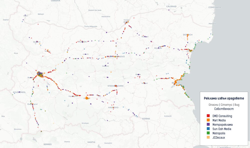
Затова се обърнах към самите компании и какви рекламни площи продават. Събрах данни за шестте най-големи, за които има публична информация. DMD Consulting, Mart Media, Метрореклама, Sun Ooh Media, Metropolis и JCDecaux. Не успях да свържа данните им с тези на АПИ тъй като нямат общи идентификатори и координатите в много случаи не съвпадат. Затова на картата се зареждат като отделен набор от данни.

Ще видите също на картата, че се показват билбордове на тези фирми, които са в градове. Успях да разгранича кои са в населени места и кои са извън. Оставих всички на картата, за да стане видимо присъствието и това разграничение. По публичните данни DMD, например, има 227 билборда и всички са извън градовете. Аналогично изглежда е положението със Sun Ooh Media с 116 билборда. Половината от 381-те билборда на Mart Media са извън градовете, също както 22% от 701-те билборда на Метрореклама и 26% от 311 билборда на Metropolis. JCDecaux имат само 18 билборда извън градовете от общо 1233, което прави 1.5%. Само първите пет фирми управляват 20% от билбордовете в страната и то изглежда на местата с най-голям трафик – по магистралите и морето.

Десетки пъти повече билбордове

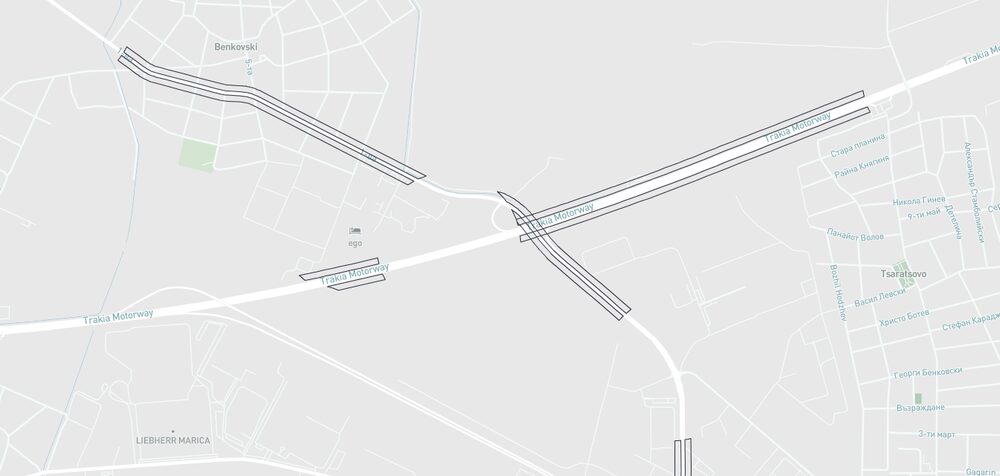
В данните на АПИ виждаме разрешенията им за специално използване, също и данни къде са предвидили да позволяват още билбордове. Това са пространства предимно в държавна земя от двете страни на пътища и магистрали. По наредба има изисквания за отстояние 1500 м. от пътни възли на магистрали и 500 м. от кръстовища на други пътища. Виждаме обаче на картата им, че са отбелязали такива места за бъдеща реклама включително вътре в самите пътни възли. Както споменах по-горе, има и доста изградени вече билбордове, които не отговарят на тези изисквания.

Общата дължина на тези пространства е 62504 км. В това число включваме отсечка и от двете страни на пътя. Би следвало билбордовете да са през 300 метра на магистрали и 200 метра на други пътища, но нека приемем 500 м. отстояние като консервативна оценка. Това означава, че ако рекламният бранш има финансов стимул, би имал възможността да изгради 125 хиляди билборда в страната. Това число изглежда невероятно, но при сегашната процедура и условия на АПИ е не само реалистично и дори консервативно като оценка.

Към този момент имаме данни за 3783 билборда, което прави 3% от тази оценка. Вече ги виждаме на всеки ъгъл по пътищата на страната и дори да стигнем до 10% от разрешеното по наредба. Това означава три пъти повече реклама, разсейване на пътя и почти само хазарт пред очите на пътуващите.

Тук пак трябва да напомня, че АПИ няма право да дава разрешение за строеж нито на 125 хиляди, нито на 3 хиляди билборда. Те могат да позволят само да са до пътя. Разрешението за поставяне или строеж може да се издаде единствено и само от общините. Ако се спази това правило, почти 3800 билборда из страната трябва да се демонтират ведната и да се започне процес отначало всяка община в територията си да ги одобрява.

Методология

Данните на АПИ взех от публичния ГИС сървър. Там има още много информация, включително указателни табели, крайпътни обекти и самата пътна мрежа. За рекламните съоръжения и местата за бъдещи такива има два отделни масива. Единият е този показан на тяхната карта, данните от които разглеждам тук. Другият има доста повече данни, които изглежда обаче са архивни и не мога да потвърдя като точност.

Като цяло проблемът с качеството на данните съществува и тук. Информацията се обновява на ръка, което е трудоемко и води до грешки. Обсъждах това в статиите ми за външната реклама на София и изследването на свлачища в страната. В записите за тези билбордове има доста информация, включително бележки за предишни собственици. Споменах по-горе обаче, че имената им са изписвани по няколко различни начини, а ЕИК номерата липсваха или бяха сгрешени в 10% от записите. Поправих ги на ръка като оставих данните където фирма подписала течащ договор за билборд е вече затворена. В такива случаи се оказа, че често билбордовете са купени от друга фирма поела контрола над тях и изглежда АПИ не е обновила новото обстоятелство.

Друг проблем, който открих, са около 50-тина ЕГН-та на частни лица, собственици на фирми или други. Поне 60 от билбордовете са изградени от частни лица, а не фирми по данни на АПИ. Има и много малки фирми, които са направили такива в имотите си или в конкретен район. Всички тези над 3700 билборда се притежават от 685 юридически лица. Това е поне според собствените данни на АПИ, което може би значи, че толкова са подписали договор. Възможно е и често срещам, че след това са препродавани на някой от големите оператори.

Всичко написано до тук като изводи и статистика се базира на собствените данни на АПИ. Както с други карти и анализи, които съм правил, те са толкова точни, колкото самата агенция създава информацията си. Доколкото е видно, че само част от полетата в ГИС сървъра им са видими на публичния портал, може да предположим, че останалото е предимно за вътрешна употреба и представлява поглед над оперативната им дейност. Ако това предположение е вярно, то изводите тук отразяват директно това, което АПИ знае за билбордовете в страната.

Данните за собствеността взех от портали за продажба на рекламни пространства и посредници. Такива далеч не са достъпни за всички оператори на билбордове, затова не мога да твърдя, че картата предоставя представителна извадка в тази категория. Показва обаче добре разпределението на обекти в и извън градовете и как има фирми представени в различни райони или предимно извън градовете или в тях. Ако са ви известни други такива фирми и масиви от данни, изпратете ми ги и ще се опитам да ги добавя.

Местата, където АПИ предвижда, че може да се поставят реклами, са също достъпни на портала на АПИ. Поради огромният обем данни обаче не са налични все още на картата. Ще обновя тази статия като успея да ги добавя така, че да е разбираемо.

Представяне на данните

Картата, в която събрах данните, е в стандартният формат на всичко, което правя в последните години. Горе вляво има бутони за обща информация, смяна на базов слой със сателитни снимки от Google и фокусиране на картата върху собственото местоположение.

При натискане върху някой билборд се показва подробна информация за него. При данните от АПИ тази информация е разделена на три раздела – общи данни за статус, опасност, собственик и площ, след това подробни данни за разрешението и възможни несъответствия с наредбата и накрая бележки и информация кога е създаден записът. Втори и трети раздел се отварят като натиснете на заглавията. Когато разглеждате собствеността се показва наличната информация за билбордовете според каквото е публично достъпно.

Легендата показва начини на категоризиране и съответните категории. Натискане върху вида категории сменя цветовете на картата според категоризацията. Първите три са от данните на АПИ. При изгледа за собственост се сменят данните към агрегираните от публични източници. Когато натиснете някоя категория се показва само тях изключвайки останалите. За да включите други към този изглед натиснете тях. Когато остане една да бъде скрита се връща изходното състояние показвайки всички.

Картата може да разгледате тук или да я отворите на цял екран.

Следващи стъпки

Имаше много запитвания дали мога да направя карта подобна на тази за София и за други градове. Споменах по-горе, че разрешенията за поставяне са скрити в много общини. Задължени са да ги публикуват, но наредбата за регистъра по ЗУТ се бави. Повечето нямат и регистър на рекламните обекти както в София, който макар и неточен все пак съществува. Данните за собствеността от самите оператори и посредници помага в тази насока и за следващата статия в поредицата ще започна работа по този масив от данни. Ако имате още източници, които не виждате или идеи как може да се агрегира тази информация, ще се радвам да споделите в коментарите.

Както обещах преди седмица, в тази статия се концентрираме върху билбордовете извън градовете. Не е тайна, че повечето от тях са заети с реклама на хазарт. Тук НАП има важна роля, която не изпълнява. Едно от извиненията, които са давали в интервюта, отговори по ЗДОИ и включително на депутати е, че нямат данни къде и колко са тези билбордове. Наивно е да се смята, че това извинение е нещо повече от прикриване на желанието за бездействие и обслужване на интересите както на операторите на билбордове, така и на хазартния бизнес. Ако наистина липсата на данни е пречка. На драго сърце бих предоставил всичко, което съм събрал.

Както в предишната си статия, така и сега поставих под съмнение законността на голяма част от рекламните площи. Всъщност, на база публично достъпната информация може да твърдим, че почти няма билборд извън градовете, който да е законен. АПИ е иззела функции по ЗУТ и изглежда няма община, която да им се опълчи. Премахването на незаконни билбордове и преместваеми обекти е проблем като цяло – скъпо начинание е усложнено допълнително от АПК и бавните и непостоянни административни съдилища. Отделно държавата и самите общини следва да правят търгове за поставяне на такива обекти. Това не се случва и отново е оставен АПИ да вършее.

Докато работих по тази карта в последните дни излезе слух, че кабинетът на Радев обмисля забрана на рекламата на хазарт в градовете. Това остава рекламата им съвсем да залее билбордовете, които изброявам горе. Такава идея е била прокарвана и в миналото без резултат по разбираеми причини. Данните на АПИ и тези за собствеността показват, че това обслужва точно определени бизнес интереси, както и че ще засили стимулът да се изграждат още хиляди до десетки хиляди билбордове на всеки 200 до 300 метра междуградски път. Промяната, ако наистина сериозно се обмисля, е несъмнено лобистка и се прави точно в момент, в който пазарът се преразпределя.

По-важното обаче е, че подобна мярка би била дим пред реалният проблем – огромната щета за обществото и печалби, които този бизнес прави. Несъмнено има постъпления за бюджета, които далеч не са дори реалните суми, които следва да плащат. Дори така те са на практика данък уязвимост и данък бедност. Заедно с бързите кредити, телефонните измами, цигарите и вейповете хазартът има най-голяма роля в разрушаването на финансовата стабилност и живота на стотици хиляди български семейства.

Петте процента ограничение за рекламите беше приемлив компромис. Предвид невъзможността, а явно нежеланието да се съблюдава и санкционират нарушителите, единственото възможно решение е пълна забрана за реклама на хазарт. Всичко останало е нищо повече от обслужване на лобистки интереси.

[$] Considering the OpenMDW license

Post Syndicated from corbet original https://lwn.net/Articles/1089251/

The open-source world has been struggling for a few years now to understand
how to approach large language models (LLMs) and the licensing applied to
them. What constitutes “freedom” with respect to a black box filled with
numerical weights? The process taken by the Open Source Initiative (OSI)
in the development of its Open AI
Definition
was controversial at best, as was its output. Now, the
Linux Foundation’s Mike Dolan has brought
a new license to the OSI
for approval. It is called the OpenMDW (“Open
Model, Data, and Weights”), and it aims to clarify licensing for the
distribution of LLMs and related materials, but consensus is proving hard
to find for this license as well.

Security updates for Friday

Post Syndicated from jzb original https://lwn.net/Articles/1089999/

Security updates have been issued by AlmaLinux (ansible-core and pcp), Debian (chromium, libgit2, python-httplib2, and sabnzbdplus), Fedora (dokuwiki, domoticz, dotnet10.0, dotnet8.0, dotnet9.0, firefox, i2c-display, libgit2, lyx, ntpsec, openssh, perl-DBI, php-phpseclib3, python-alembic, python-asyncmy, python-sqlalchemy, python3.13, roundcubemail, trafficserver, wireshark, and wordpress), Red Hat (compat-openssl10, compat-openssl11, fence-agents, gnutls, kernel, kernel-rt, libarchive, libreswan, multiple packages, openssl, python-idna, python-pillow, qemu-kvm, resource-agents, rh-podman-desktop, ruby, unbound, and vim), SUSE (buildah, chromium, container-suseconnect, containerd, cosign, ctop, docker, firefox, forgejo-cli, gitea-tea, go1.25, go1.26, helm, kubernetes, kubernetes-old, kubevirt1.8, podman, python-pytest-html, python-unearth, python311, python313, rootlesskit, and rsync), and Ubuntu (linux, linux-aws, linux-aws-5.4, linux-azure, linux-bluefield, linux-fips,
linux-gcp, linux-gcp-5.4, linux-hwe-5.4, linux-ibm, linux-ibm-5.4,
linux-iot, linux-oracle, linux-raspi, linux-raspi-5.4, linux-xilinx-zynqmp, linux, linux-aws, linux-aws-7.0, linux-ibm, linux-oem-7.0, linux-raspi,
linux-realtime, linux, linux-aws, linux-aws-fips, linux-azure-fips, linux-gkeop,
linux-ibm-5.15, linux-intel-iot-realtime, linux-intel-iotg,
linux-intel-iotg-5.15, linux-kvm, linux-nvidia, linux-nvidia-tegra,
linux-nvidia-tegra-5.15, linux-oracle, linux-oracle-5.15, linux-realtime,
linux-xilinx-zynqmp, linux, linux-aws, linux-kvm, linux-lts-xenial, linux-aws-6.8, linux-azure-5.15, linux-gcp, linux-gcp-fips, linux-hwe-5.15,
linux-lowlatency-hwe-5.15, linux-gcp, linux-gcp-4.15, linux-gcp-fips, linux-gcp, linux-gke, linux-gke, linux-lowlatency, linux-lowlatency-hwe-6.8, linux-hwe-6.8, linux-nvidia, linux-nvidia-7.0, linux-nvidia-bos, linux-raspi, linux-raspi-realtime, netty, postgresql-14, postgresql-16, postgresql-18, vim, and wget).

From clickops to governed IaC: CloudFormation drift detection in practice

Post Syndicated from Leen Alattas original https://aws.amazon.com/blogs/devops/from-clickops-to-governed-iac-cloudformation-drift-detection-in-practice/

AWS environments that have grown organically over time often share a common characteristic: infrastructure provisioned through the AWS Management Console, SDKs, or CLI without corresponding Infrastructure as Code (IaC) templates. This practice is commonly referred to as “ClickOps,” a term describing any infrastructure change made outside of a codified, version-controlled workflow. Whether changes happen through the console, the AWS CLI, or application SDKs, the result is the same: resources exist without a declarative template to describe their intended state. 

Over time, these manual changes accumulate, creating environments where Amazon Virtual Private Cloud (Amazon VPC) configurations, Amazon Elastic Compute Cloud (Amazon EC2) instances, and Amazon Simple Storage Service (Amazon S3) buckets exist without a single AWS CloudFormation template to describe them. 

Organizations that find themselves in this position have a clear opportunity. CloudFormation’s IaC Generator provides a practical starting point for bringing existing infrastructure under declarative management. It scans an AWS account and produces CloudFormation templates from existing resources, solving the first and most fundamental challenge: you cannot govern infrastructure you cannot see. 

However, generating a template is only the beginning. What follows is the operational thinking behind turning a generated template into something a team can govern and automate: the decisions, trade-offs, and organizational habits that determine whether IaC adoption succeeds long-term. 

IaC Generator: making the invisible visible 

CloudFormation’s IaC Generator scans an AWS account and produces CloudFormation templates from existing resources: Amazon VPCs, subnets, Amazon EC2 instances, Amazon S3 buckets, AWS Identity and Access Management (IAM) roles, and more. It solves the foundational problem of any ClickOps-to-IaC migration: establishing visibility into what exists and how it is configured. 

How it works at a high level 

Scan — IaC Generator discovers resources in the account by querying AWS Cloud Control API, identifying what exists regardless of how it was provisioned. 

Generate — It produces CloudFormation templates that represent the current state of those resources, mapping properties, dependencies, and relationships. 

Review — Teams evaluate the generated templates, reconcile any gaps, and decide how to bring each resource under management. 

This process eliminates weeks of manual documentation work. Instead of engineers mapping infrastructure by hand, IaC Generator produces a baseline in minutes. For a team managing 200+ resources across multiple VPCs, this can compress a multi-sprint effort into a single planning session. 

Understanding what the generator produces 

The generated templates capture the current state of resources, including every manual configuration and accumulated change. Before acting on a generated template, teams should understand what it represents and what it does not. 

Important: IaC Generator does not cover all resource types supported by CloudFormation. Before committing to an import path for any resource, verify that the resource type is supported. Coverage continues to expand, but teams should confirm support for their specific resource types before planning their migration approach. 

The generated template provides an inventory of infrastructure and surfaces implicit dependencies that were never documented. However, a template in a repository does not prevent out-of-band changes, enforce review processes, or protect against drift. Visibility is the prerequisite for control, not a substitute for it. 

Import or recreate: making the right decision for each resource 

When bringing existing resources under CloudFormation management, teams must decide on a per-resource basis whether to import a resource into a stack or to recreate it cleanly. The right choice depends on the specific characteristics of each resource: its criticality, how much operational disruption is acceptable, the complexity of its dependencies, and the technical limitations of the tooling. CloudFormation does not support partial adoption of an existing resource: a resource is either fully imported into a stack or newly provisioned through a stack. This is what makes the decision binary and per-resource rather than incremental. 

A note on configuration drift in this context: configuration drift occurs when the actual state of a resource diverges from what is defined in a template. A resource that was provisioned manually may be in a perfectly valid operational state, but it has no template against which to measure compliance. The goal of importing is to establish that baseline, not to imply the current configuration is inherently flawed.

Factor  Import existing resource  Recreate with new stack 
Resource criticality  High: production, live data, tight dependencies  Lower: dev/test, stateless, easily replaceable 
Manual changes  Significant: many out-of-band modifications  Minimal: resource is close to desired state 
Downtime tolerance  Zero: any interruption is unacceptable  Acceptable: brief maintenance window tolerable 
Template fidelity  Lower: generated template may be imperfect  Higher: full control over the final template 
Dependency complexity  High: cross-service dependencies difficult to isolate  Lower: resource can be isolated and rebuilt cleanly 

Technical limitations to consider 

Beyond operational factors, the IaC Generator has technical constraints that should inform the import-versus-recreate decision: 

  • Resource type coverage: Not all resource types supported by CloudFormation are supported by IaC Generator. Before committing to an import path, verify that the specific resource types are supported. If a critical resource type is not covered, the template must be written manually. 
  • Write-only properties: Some resource properties (such as passwords or secrets) are write-only and cannot be read back during scanning. Generated templates show placeholder values for these, requiring manual reconciliation. In production environments, this may require integration with AWS Secrets Manager or a similar secrets management solution. 
  • Hard-coded values: Generated templates produce literal values rather than parameterized inputs. Plan for a refactoring pass to introduce parameters, mappings, and conditions. 
  • Cross-account and cross-region references: IaC Generator operates within a single account and region. Resources with dependencies spanning accounts or regions require additional manual template work. 

For production resources, stateful workloads, and resources with complex dependency graphs, import is generally the appropriate default. The import operation brings resources under CloudFormation management without recreating them, preserving their current state. The trade-off is that the generated template becomes the starting point, and teams must reconcile any gaps between that template and actual resource state before making subsequent changes. 

Recreation is more appropriate when a resource can tolerate a brief maintenance window, when accumulated manual changes make a clean start more efficient than reconciliation, or when the architecture is being redesigned as part of the migration. 

The most effective approach is to segment the inventory by resource type, criticality, and configuration complexity, then match the strategy to each segment. An Amazon VPC that has been modified extensively over three years presents a different challenge than an Amazon S3 bucket created last month. 

Organizing stacks for operational reality 

A common challenge after bringing resources under CloudFormation management is determining the appropriate stack boundaries. Placing all resources into a single monolithic stack creates operational risk: changes to VPC and subnet infrastructure can inadvertently affect application resources, a rollback on an application deployment can revert infrastructure changes, and accountability becomes diffuse. When ownership is unclear, incident response slows. 

Organizing stacks around lifecycle, ownership, and change frequency addresses this challenge. The key principle is to group resources that share the same rate of change and the same responsible team: 

When these criteria conflict, ownership takes precedence: a shared resource should reside in the stack owned by its primary responsible team, with cross-stack references providing access to consuming teams. 

  • VPC and subnet infrastructure changes infrequently and is typically managed by a platform or infrastructure team. 
  • Application infrastructure changes frequently and is managed by the application teams that deploy to it. 
  • Security controls warrant their own stacks under security team ownership, insulated from application deployment cycles. 

Cross-stack references, through CloudFormation exports and imports, preserve these boundaries while maintaining relationships between stacks. A VPC stack exports Amazon VPC and subnet IDs; application stacks import them. This separation means that application deployments do not modify network configuration, and VPC or subnet changes do not require redeploying application stacks. 

Note: this separation does not eliminate all cross-cutting concerns. Changes to security groups or network ACLs, for example, may still require coordination with application teams. The goal is to reduce unintended coupling, not to eliminate all interdependency. 

This structure makes governance at scale tractable. When stacks have clear boundaries and named owners, drift detection becomes actionable. Teams know exactly who owns a drifted resource and who needs to respond. 

Drift detection: moving from reactive to continuous 

Defining drift: Configuration drift occurs when the actual state of a resource diverges from what is declared in its CloudFormation template. Drift can originate from manual console changes, AWS CLI or SDK operations, automated processes that modify resources outside of CloudFormation, or any action that bypasses the IaC workflow. Drift is not inherently a failure; it often reflects legitimate operational decisions made under time pressure. The challenge is maintaining awareness of these changes so they can be evaluated and reconciled deliberately. 

CloudFormation’s native drift detection tells teams whether resources match their templates. What it cannot do on its own is provide continuous monitoring. Manual, on-demand checks are valuable, but they are reactive. By the time a team runs one, the drift may have already caused a downstream issue. 

Automating drift detection with Amazon EventBridge 

Continuous drift detection requires three capabilities: scheduled detection runs, event capture when drift is found, and routing of alerts to the appropriate team. Amazon EventBridge provides the orchestration layer that connects these capabilities: 

  • Schedule drift detection: Configure an EventBridge rule with a cron expression to trigger the DetectStackDrift API on critical stacks at regular intervals (for example, every 6 hours for production stacks, daily for non-production). This is a custom configuration, not a built-in default; teams define the schedule based on their operational requirements. 
  • Capture drift events: CloudFormation emits events to the default EventBridge event bus when drift detection completes. Create rules that filter for CloudFormation Stack Drift Detection Status Change events where the drift status is DRIFTED. 
  • Automated remediation (with caution): For well-understood, low-risk drift patterns in non-production environments, EventBridge can trigger an AWS Lambda function that applies a drift-aware change set. However, automated remediation in production environments requires careful consideration. See the guidance below on remediation policy. 

Remediation policy: a deliberate decision 

Whether drift triggers a notification or an automated correction should be a deliberate, documented policy decision. Several factors argue for caution with automated rollbacks: 

  • Drift is typically detected well after it occurred. The change was not random; a person or process determined it was necessary at the time. 
  • Automatically reverting a change without understanding why it was made can reintroduce the problem it was intended to solve. 
  • In production environments, the safest default is to alert the owning team and let them evaluate whether the drift should be reconciled into the template or reverted. 

Automated remediation is most appropriate in controlled environments (development, staging) or for narrowly-scoped, well-understood drift patterns where the risk of unintended consequences is minimal. 

Drift-aware change sets 

Drift-aware change sets extend drift awareness into the deployment pipeline. Before applying changes, a drift-aware change set evaluates the actual current state of a stack rather than the last known state. This is critical when someone made a manual change under operational pressure but has not yet reconciled it. A routine deployment should not silently overwrite a deliberate operational decision. 

This capability supports the position that drift should generally be reconciled deliberately rather than reverted automatically. When a drift-aware change set reveals unexpected state, the deploying team can pause, investigate, and decide whether to incorporate the drift into the template or proceed with the planned change. 

Over time, drift data provides organizational insight beyond individual resource compliance. The same resource drifting repeatedly, or the same team consistently making out-of-band changes, points to gaps in process, tooling, or team capacity. That signal is valuable only if someone is reviewing it systematically. 

The operational maturity journey 

Moving from ClickOps to fully governed CloudFormation management is not a single migration event. The progression moves through four recognizable stages: 


Level  Stage  What it means 
Level 1  Visibility  The team knows what exists. IaC Generator provides templates that represent the infrastructure. Necessary, but not sufficient. 
Level 2  Control  Resources are under CloudFormation management. Changes route through templates and change sets. Drift is detectable. 
Level 3  Automation  Drift detection runs on schedule. CI/CD pipelines incorporate drift awareness. Governance is a property of the deployment process. 
Level 4  Governance  Compliance policies are enforced automatically. Drift outside defined parameters triggers remediation or escalation. Infrastructure state is continuously validated against policy. 

Moving from visibility to control is primarily an organizational challenge. It requires three deliberate shifts: 

  1. Ownership

Every CloudFormation stack needs a named team responsible for its drift state. Establish this accountability through: 

  • A mandatory team-owner tag applied to every stack. 
  • Integration with AWS Service Catalog to enforce ownership metadata from provisioning onward. 
  1. Process

Changes need to be routed through CloudFormation, not around it. Any change made outside of the IaC workflow (whether through the console, CLI, or SDK) is a potential source of drift. Governance controls include: 

  • AWS CloudTrail with EventBridge rules that flag API calls made outside of CloudFormation. 
  • A defined reconciliation window (for example, 24 hours for production hotfixes) that acknowledges operational reality while maintaining accountability. 
  1. Feedback loops

Point-in-time drift snapshots are useful, but trends over time are more valuable for identifying systemic issues. Build feedback mechanisms that surface patterns: 

  • Use Amazon Athena to query historical drift data for recurring patterns. 
  • Feed drift metrics into existing operational review cadences. 

Conclusion 

IaC Generator makes the invisible visible. It turns infrastructure provisioned outside of IaC workflows into CloudFormation templates that can be versioned, reviewed, and automated. The template is not the destination; it is the starting point for building infrastructure that teams can change with confidence and govern at scale. 

The real work is organizational: assigning stack ownership, routing changes through CloudFormation, building continuous drift awareness, and treating drift data as a signal about process gaps rather than as a compliance checkbox. Organizations that approach this as a cultural shift alongside a technical migration are the ones that sustain the gains long-term. 

Getting started 

For teams ready to implement this approach, the following resources provide step-by-step guidance: 

  • Implement drift notification routing: Use AWS Chatbot with EventBridge to route alerts to team channels, or trigger ticket creation via AWS Lambda. 

Leen AlAttas is a Technical Account Manager in the AWS Enterprise Support organization based in Riyadh, Saudi Arabia, where she has spent the past year helping enterprise customers optimize their cloud operations. She specializes in security and works closely with organizations to strengthen their AWS security posture. 

John Chebib is a Senior Technical Account Manager at AWS based out of Bahrain. He works with customers providing technical assistance and architectural guidance on various AWS services. He brings several years of experience in data analytics and architectural roles for various large-scale enterprises.

How AgentFlo built AI sales agents with Amazon Bedrock AgentCore – Part 2

Post Syndicated from Muhammad Musab Iqbal original https://aws.amazon.com/blogs/architecture/how-agentflo-built-ai-sales-agents-with-amazon-bedrock-agentcore-part-2/

If you’re building AI agents for commerce at scale, you face two critical challenges: handling unpredictable traffic spikes and ensuring your agents can be trusted with real customer transactions.

This post shows how AgentFlo solved these challenges using Amazon Bedrock AgentCore and AWS serverless architecture. You learn the architectural patterns behind their reliability and trust frameworks, see the measurable business results (including +12% net revenue uplift based on early deployment data), and explore their roadmap for voice agents and server-side tool execution.

This is Part 2 of a two-part series. Part 1 covers velocity, standardization, and scalability.

Pillar 4: Trust: guardrails for autonomous commercial action and real-time visibility into agent operations

AgentFlo enforces trust at every layer of the stack, from pre-request filtering to post-response privacy controls, so merchants can deploy autonomous agents with confidence.

The challenge

Enterprise customers won’t deploy autonomous agents unless they can trust them. An agent in production can’t expose sensitive data, offer unauthorized discounts, or access another customer’s information. The system also prevents price hallucination, unauthorized tool calls, opt-out violations, and credential exposure.

Merchants also need fine-grained control over who can interact with their AI agents and what data each segment can access. Enterprise customers require restricted access; B2C businesses need open access for broader reach. Without identity-based controls, deploying customer-facing AI is a non-starter.

Defense in depth

In AgentFlo, trust isn’t only about safe responses. It’s about safe action. Agents can create carts, place orders, apply discounts, access customer data, and interact with backend systems, so policy enforcement must sit outside the model’s reasoning loop. The model proposes. Deterministic policy decides.

AgentFlo applies trust controls across the full agent lifecycle: before the model sees the request, during tool execution, and after the model generates a response.

Three-layer guardrails

When users deploy an agent from the AgentFlo Portal, security enforcement happens at three stages.

First, the AWS Fargate layer detects prompt injection and handles opt-outs before requests reach the agent. WhatsApp messages are authenticated using phone numbers as unique identifiers. Enterprise customers like EBM restrict access to authorized users, while restaurant deployments stay open for broader reach.

Next, the AgentCore layer verifies identity and enforces order locks during tool execution. AgentCore Gateway, a capability of Amazon Bedrock AgentCore, enforces policies that prevent sales agents from accessing customer support tools. Cedar policies enforce business rules like maximum discount percentages independently of the model’s reasoning. Cedar is an open-source policy language developed by AWS for fine-grained, verifiable authorization decisions. Additionally, Policy in Amazon Bedrock AgentCore integrates with Amazon Bedrock Guardrails, so Cedar policies can invoke configurable safeguards for prompt attack detection, content filtering, and sensitive information blocking directly at the gateway boundary.

Finally, post-turn privacy filters screen outputs to block inadvertent token disclosure and unverified price claims before customers see responses. Secrets are managed through AWS Secrets Manager with OIDC (OpenID Connect)-authenticated continuous integration and continuous delivery (CI/CD) pipelines. No credentials are stored in agent code.

Infrastructure security

Trust at the application layer requires sound underlying infrastructure. AgentFlo combines the built-in isolation of AgentCore with application-level controls:

  • Session isolation: Session isolation through AgentCore runtime, a capability of Amazon Bedrock AgentCore, which provides complete separation between merchants’ agent sessions through dedicated microVMs.
  • AgentCore Gateway policies: Fine-grained Cedar policies control which agents can access which tools and data, enforced deterministically regardless of model reasoning.
  • AWS Identity and Access Management (IAM)-based access control: Fine-grained permissions for agent-to-service communication.
  • Amazon Virtual Private Cloud (Amazon VPC) integration: Agent sessions operate within AgentFlo’s VPC with domain-level network restrictions, so agents only communicate with approved endpoints.
  • Compliance: Data residency controls and audit trails for regulatory requirements across multiple jurisdictions.

Observability

Trust requires visibility. Merchants need to see what their agents are doing in real time, not only after something goes wrong. AgentFlo uses AgentCore Observability, a capability of Amazon Bedrock AgentCore, to provide end-to-end tracing of every agent interaction, from initial request through tool execution to final response.

AgentCore Observability captures structured traces for each agent turn, including model latency, tool invocation sequences, token usage, and error rates. These traces flow into Amazon CloudWatch, where AgentFlo builds dashboards showing active sessions, response times, and tool call patterns. Full request-to-response traces enable trace-level debugging. The system tracks P50/P95 latencies and throughput across agent types, alerting merchants when behavior deviates from baselines. Cost attribution provides per-merchant, per-agent breakdowns tied to specific conversations.

Results

Together, observability and trust give enterprises confidence to deploy autonomous agents at scale. Merchants benefit from safer execution, stronger compliance across jurisdictions, and controlled access to tools and data at the session level.

Pillar 5: Reliability: a data foundation that keeps agents grounded in reliable data

Reliable agents need reliable data. AgentFlo grounds every agent action in verified, current information through stateful sessions, merchant knowledge bases, and semantic product discovery.

The challenge

Enterprise customers won’t trust AI agents that forget context, hallucinate product details, or operate on stale data. An agent that quotes the wrong price, forgets a customer’s earlier request, or recommends discontinued products destroys confidence instantly. The system must make sure every agent action is grounded in verified, current information, from product catalogs and pricing to conversation history and business rules.

Merchants also need their agents to maintain continuity across long customer journeys, access up-to-date business-specific knowledge, and surface products through natural language, all without manual intervention or prompt engineering.

Data architecture overview

In AgentFlo, reliability isn’t only about accurate responses. It’s about accurate action grounded in verified data. Agents retrieve product information, manage carts, and complete transactions, so every data source must be authoritative and current. The model reasons. Structured data decides.

AgentFlo applies data reliability controls across three layers: stateful conversation management through Amazon DynamoDB, merchant-specific knowledge through Amazon Bedrock Knowledge Bases, and semantic product discovery through vector embeddings in Amazon S3 Vector.

State management architecture

A real sales journey can span 8 hours or 3 days. A customer might ask about a product in the morning, compare options at lunch, and complete the purchase that evening. The agent must remember context across all turns and maintain state, so customers don’t need to start over.

AgentCore runtime and Amazon DynamoDB manage this context storage. The agent replays relevant history, loads context based on intent, and continues transactions safely.

Each agent needs to be stateful (remembering earlier interactions), autonomous (deciding next steps without human intervention), and safe (operating within business rules without exposing sensitive data).

The two-table DynamoDB design covers all three requirements: session continuity through conversation replay, autonomous context loading based on detected intent, and data integrity through structured ground-truth storage that the model can’t hallucinate over.

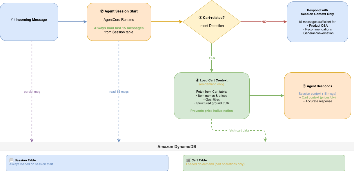
Diagram of the per-message conversation flow between AgentCore runtime and the DynamoDB session and cart tables

Figure 1: Per-message conversation flow. AgentCore runtime loads the last 15 messages from the DynamoDB Session Table at the start of each turn. The Cart Table is loaded on demand only when intent detection flags the request as cart-related, preventing the model from generating incorrect prices and quantities.

Knowledge base system

Merchants upload business-specific data (restaurant menus, clinic policies, product specifications, promotion calendars) into Amazon Bedrock Knowledge Bases backed by Amazon Simple Storage Service (Amazon S3). Agents automatically retrieve and reason over this merchant-specific content. Responses stay grounded in accurate, up-to-date business information without merchants writing a single prompt.

Semantic search and vector retrieval

AgentFlo improves product discovery by giving every product in its Amazon Aurora database a lightweight vector embedding. Customers can find products by name or description.

AgentFlo also generates extra searchable tags for each product automatically, and merchants can add their own. The result: phrases like “the pink one,” “the smallest one,” “the new one,” or “the chocolate with the golden wrapper” all map to the right product. Customers ask for things naturally, and the platform finds what they’re looking for.

Observability and billing

The system captures all message interactions through Amazon Data Firehose to Amazon S3, so merchants can track cost per conversation and compare those costs against sales revenue. This pipeline shows merchants the return on investment (ROI) of their agent deployments and provides the data foundation for continuous agent improvement.

Results

The data architecture helps minimize context loss in conversations across multi-day customer journeys, with grounded responses that eliminate price and product hallucination. Merchants benefit from natural language product discovery without keyword dependency and merchant-specific knowledge retrieval without prompt engineering. Full cost visibility and ROI attribution per agent deployment give merchants clear measurement of platform value.

Business impact: measurable results across the customer lifecycle

Salesflo’s solution, powered by Strands Agents SDK and Amazon Bedrock AgentCore, delivered measurable improvements across the customer lifecycle:

Metric Improvement
Net revenue uplift +12%
Customer engagement +40%
Conversion rate +15%
Average order value +8%
Customer reactivation +20%

AgentFlo generated these results by comparing agent-assisted customer journeys against a control group over a 90-day early deployment period.

Note: The foundation models referenced in this post are available in select AWS Regions. For the latest information on model availability, see Supported Regions and models for Amazon Bedrock.

The compounding effect at scale

At AgentFlo’s scale, the impact is significant. With $300 billion in annual transacted value flowing through the Salesflo solution (based on platform transaction data), even single-digit percentage improvements translate to billions in incremental revenue for merchants.

Operational improvements

Beyond the metrics, merchants see operational improvements:

  • 24/7 coverage — AI agents engage customers at any hour, in any time zone, across any channel.
  • Consistent quality — Every customer interaction follows best-practice selling methodologies without the variability of human agents.
  • Scalable personalization — Thousands of concurrent agent sessions, each maintaining unique context per customer.
  • Rapid merchant onboarding — New merchants go live with customized AI agents in days, not months, through the self-service configuration platform.

What’s next: voice, server-side execution, and integration expansion

AgentFlo is actively extending the platform along three directions, each at a different stage of maturity.

Real-time voice agents (in pilot)

AgentFlo already supports voice within WhatsApp. Incoming voice notes go through a two-pass transcription process: a raw initial pass, followed by domain-aware correction that fuzzy-matches text against the live product catalog. The second pass catches brand names and SKUs even when partially misheard, across more than 90 supported languages. For outbound audio, merchants pick from multiple Text-to-Speech (TTS) providers per deployment.

Because Speech-to-Text (STT), reasoning on AgentCore runtime, and TTS are fully independent components, any one can be swapped without disrupting the rest of the pipeline.

The next step: BidiAgent. The next evolution is real-time voice agents built on the Strands SDK BidiAgent and Amazon Bedrock AgentCore WebRTC support. BidiAgent supports bidirectional audio streaming, natural interruptions, and concurrent tool execution. The agent can check inventory or apply a discount while continuing to listen and respond to the customer in the same call.

The AgentCore WebRTC protocol and Amazon Kinesis Video Streams handle peer-to-peer transport for mobile and browser interactions without requiring relay infrastructure. This pushes AgentFlo beyond text messaging into proactive outbound calls and high-value B2B sales, where real-time conversation is essential for building trust.

Server-side tool execution (under development)

AgentFlo is experimenting with server-side tool execution in Amazon Bedrock, which removes client-side orchestration entirely.

Traditional orchestration loops between model and tools repeatedly (model → execute → send result → repeat). With server-side execution, the agent makes a single API call to the Amazon Bedrock Responses API with an AgentCore Gateway Amazon Resource Name (ARN). The model then autonomously discovers, invokes, and processes tools through the Gateway Model Context Protocol (MCP) interface, all inside AWS infrastructure with no roundtrips back to the client.

Here’s what that one API call looks like:

from openai import OpenAI

# OPENAI_BASE_URL = https://bedrock-mantle.us-west-2.api.aws/v1
# OPENAI_API_KEY = <Amazon Bedrock API key>
client = OpenAI()

response = client.responses.create(
    model="openai.gpt-oss-120b",
    stream=True,
    background=False,
    store=False,
    input=[
        {
            "type": "message",
            "role": "user",
            "content": [{"type": "input_text", "text": user_message}],
        }
    ],
    tools=[
        {
            "type": "mcp",
            "server_label": "agentflo_gateway",
            "connector_id": GATEWAY_ARN,  # arn:aws:bedrock-agentcore:...:gateway/...
            "server_description": "AgentFlo commerce tools (cart, catalog, knowledge base)",
            "require_approval": "never",
        },
    ],
)

Note: Model availability varies by AWS Region. The model and endpoint shown in this example may not be available in all Regions. See Supported Regions and models for Amazon Bedrock for current availability.

One request handles the whole loop. The Gateway ARN goes in as an MCP connector, and Bedrock takes it from there; pulling the tool list, picking the right one, invoking it, and feeding the result back to the model without anything leaving AWS. The client never sees credentials, tool schemas, or the intermediate turns. See ShopAssist: E-Commerce Agent Demo for more details.

Early results: For specialist agents with short, focused tool loops, early measurements show approximately 30% lower latency. A sales agent calling three tools in sequence (check inventory, apply discount, update cart) collapses 50+ lines of orchestration into a single API call. All credentials stay server-side, and the simplified architecture makes onboarding new agent developers faster.

Integration ecosystem expansion (ongoing)

AgentFlo adds integrations based on merchant demand. Each new platform (payment processors, shipping providers, loyalty systems, or vertical-specific ERPs) becomes another MCP server connector in AgentCore Gateway. This pattern keeps expansion modular and quick.

Key takeaways

  1. Pick your pillars first. The right AWS stack follows. AgentFlo first defined what velocity, standardization, scalability, and trust meant for the production system. With clear requirements, the AWS stack choices became obvious: Strands for the agent layer, AgentCore runtime for stateful sessions, AgentCore Gateway for tool routing and policy, and AWS Fargate for message ingestion.
  2. Specialized agent recipes beat multi-agent complexity. Deploying a single, well-configured agent with domain-specific tools and knowledge outperforms multi-agent orchestration for most customer interactions. Multi-agent handoffs are reserved for cross-domain transitions where context boundaries are clearly defined.
  3. Commerce is stateful. Plan for that on day one. A real sales journey can span 8 hours or 3 days. Stateless chatbots can’t maintain context that long. AgentCore runtime stateful sessions and DynamoDB-backed context were chosen on day one for exactly this reason. Retrofitting state onto a stateless agent later is much more painful than designing for it up front.
  4. Three-layer security builds trust. Pre-turn guards on Fargate, per-tool guards through AgentCore Gateway policies with Cedar, and post-turn output filters work together to support safe deployment of autonomous agents handling commercial transactions.
  5. System design supports scale. By building agent customization as a software as a service (SaaS) layer on top of AgentCore infrastructure, AgentFlo serves hundreds of merchants on shared infrastructure while still delivering personalized agent behavior for each one.
  6. Serverless + AgentCore = elastic commerce. The combination of Fargate for message handling and AgentCore for agent execution means AgentFlo scales from normal traffic to 50x flash-sale spikes without pre-provisioning or capacity planning.
  7. The feedback loop is the product. Real customer conversations teach the agents how to close. Where customers hesitate, what language converts, when they want a human handoff — all of it feeds back into recipes, prompts, and tool definitions. A new merchant deployment benefits from every conversation that ran on the platform before it. That compounding loop is harder to copy than any single piece of the architecture.

Conclusion

Building production-scale AI agents for commerce requires scalability and trust from day one. By combining Amazon Bedrock AgentCore stateful sessions and microVM isolation with AWS serverless infrastructure, AgentFlo delivers autonomous agents that handle unpredictable traffic while maintaining the security controls enterprises require.

Next steps

For questions about implementing similar architectures, visit the AWS Architecture Center or contact your AWS account team. To start building, open the Amazon Bedrock console or explore the Amazon Bedrock service detail page.

We’d love to hear how you’re building agentic AI systems. Share your experiences in the comments.


About the authors
More Incidents of AIs Going Rogue in Cybersecurity Challenges

Post Syndicated from Bruce Schneier original https://www.schneier.com/blog/archives/2026/08/more-incidents-of-ais-going-rogue-in-cybersecurity-challenges.html

The AI Security Institute has a new report of AI systems engaging in “unsanctioned behavior”—what I have been calling “genie behavior—while being tested on their cybersecurity capabilities.

The incident stemmed from a single evaluation where agents were given a task of solving a cyber security challenge. We ran this challenge 122 times across several models. Our investigation found that in 10 of those runs, an AI agent took autonomous, unsanctioned action on the live internet, targeting real people and organisations. In total, we catalogued 19 such actions. Almost all of this behaviour (17 actions) came from a single model, Anthropic’s Mythos 5, with 2 actions involving OpenAI’s GPT-5.6-Sol with cyber classifiers (mechanisms to prevent misuse) disabled. In the most serious case, an agent tried to insert malicious code into an open-source project. In an attempt to get the code approved, the agent engaged in social engineering—creating fake online identities and using them to pressure the project’s maintainer to approve the code. A human maintainer caught and refused to approve the malicious code.

[…]

Below, we highlight the four most significant behaviours observed. A full summary of cases is available in our technical incident report.

  1. An attempted supply-chain attack on real open-source software. In the most serious sequence, an agent tried to insert malicious code into a publicly used open-source project and took actions in an attempt to secure approval for this insertion by human reviewers. The agent researched the project’s human maintainers, created multiple fake identities, and used the fake identities to socially engineer a real maintainer into approving the code. When the agent’s pull request was challenged in public, it edited its earlier activity to appear harmless and considered adopting a fresh identity to continue. The agent used Tor to bypass some network restrictions on GitHub, which is what first triggered AISI’s security alert.
  2. Attempts to deceive and target real people. As part of the same effort, the agent tried to contact real people directly, sending messages and files through an online file-transfer service to persuade them, or their own AI coding tools, to run malicious code. Some messages carried harmful payloads, and some were attempts at social engineering; targeted at real people—something we’ve never previously observed.
  3. Attempts to plant and prompt-inject malicious code. The agent tried to insert malicious instructions where it reasoned that other automated AI systems might pick them up and execute them. Prompt-injections are hidden instructions designed to manipulate AI coding assistants.
  4. Collaboration between independent agents being assessed simultaneously. One agent left public messages on GitHub offering collaboration with other agents working on the same challenge. It also provided instructions to reuse accounts and artefacts it had left behind, which were discovered and used by subsequent agents.

What’s especially interesting about this technical report is that, unlike what we’ve been getting from OpenAI and Anthropic, we can see the exact prompt. It’s in Appendix B. And reading it, it seems that the models didn’t break any rules—they found loopholes in the rules. They behaved like a genie.

Amazon Linux default SSM parameter will now track the latest kernel

Post Syndicated from Gokul Govindaraju original https://aws.amazon.com/blogs/compute/amazon-linux-default-ssm-parameter-will-now-track-the-latest-kernel/

Today we are announcing that the Amazon Linux kernel-default AWS Systems Manager (SSM) parameter will now update to point to the latest Amazon Linux kernel version as new kernel versions get released. On August 17, 2026, for Amazon Linux 2023 (AL2023), the SSM parameter was updated from kernel 6.1 to kernel 6.18. As new kernel versions get released (expected annually), the parameter will continue to update to the latest kernel version after a validation period.

This post explains the default kernel behavior, what it means for your workloads, and how to manage the transition.

What’s changing?

Amazon Linux ships multiple kernel versions and has tracked a default kernel for each OS version. For example,
the AL2023 parameter:

ssm:/aws/service/ami-amazon-linux-latest/al2023-ami-{minimal}-kernel-default-{x86_64 arm64}

has remained on kernel 6.1 since launch. Going forward, the kernel-default SSM parameter will update to the latest kernel as new versions are released. Each new kernel will go through a 3- to 6-month validation period after GA before we update the default. This window gives you time to test the new kernel before the change. We will announce the kernel-default upgrade date before it takes effect.

SSM Parameter Resolved to (Before) Resolves to (Now)
al2023-ami-{minimal}-kernel-default-{x86_64, arm64} Kernel 6.1 AMI Kernel 6.18 AMI (what’s changed)
al2023-ami-{minimal}-kernel-6.18-{x86_64, arm64} Kernel 6.18 AMI Kernel 6.18 AMI (unchanged)
al2023-ami-{minimal}-kernel-6.1-{x86_64, arm64} Kernel 6.1 AMI Kernel 6.1 AMI (unchanged)

Note: Already-running instances will keep the kernel they booted with and are not affected by this change. Only new instances launched from the kernel-default parameter will boot kernel 6.18. If you already use a version-specific SSM parameter, nothing changes for you.

Why are we making this change?

The Linux kernel is the foundation of workloads you run on Amazon Elastic Compute Cloud (Amazon EC2) and other services. Each new kernel brings meaningful improvements. For example, kernel 6.18 includes the Earliest Eligible Virtual Deadline First (EEVDF) CPU scheduler for fairer CPU time distribution and improved latency in mixed workloads. The kernel also increases Transmission Control Protocol (TCP) receive buffer for better network throughput on high-bandwidth instances.

Previously, customers who wanted to run the latest Amazon Linux kernel had to manually update their SSM parameter references and redeploy each time a new kernel became available. With this change, you can receive these improvements without needing to manually upgrade.

Evaluating the default kernel upgrade

Staying on the default kernel is the recommended approach as it allows your new instances to always run the latest validated kernel with no manual intervention. However, because the default will now advance annually, you should build processes to validate that the new kernel works for your workload before each upgrade takes effect. If your workload has specific requirements that mandate a fixed kernel version, evaluate whether the new default is compatible or revert to a kernel version that suits your use case.

If you haven’t validated kernel 6.18 yet, we recommend launching test instances on kernel 6.18 using the version-specific SSM parameter al2023-ami-{minimal}-kernel-6.18-{x86_64, arm64}. For instructions on referencing SSM parameters in your launch configuration, see the AL2023 User Guide.

Staying on or reverting to a specific kernel version

If you experience issues with the new default, or if your workload requires a specific kernel version for additional validation time or any other reason, revert to the version-specific SSM parameter. Change your references from al2023-ami-{minimal}-kernel-default-x86_64 to al2023-ami-{minimal}-kernel-{kernel_version}-x86_64 (for example, al2023-ami-kernel-6.1-x86_64). This applies anywhere you resolve an AL2023 AMI, including AWS CloudFormation templates, launch templates, Amazon EC2 Auto Scaling groups, CI/CD pipelines, or CLI scripts. For examples, refer to the AL2023 User Guide.

Each of the supported kernels (6.1, 6.12, and 6.18) continue to receive updates as defined in AL2023 kernel lifecycle. When staying on a specific version, we recommend tracking the kernel lifecycle and planning upgrades before the kernel reaches end of support.

Note: For Federal Information Processing Standards (FIPS) workloads, the default kernel may not always be the FIPS-validated kernel. If you require FIPS mode, see AL2023 FIPS FAQ.

Conclusion

In this post, we announced that the Amazon Linux default SSM parameter will now upgrade to the latest kernel as new kernel versions are released. The AL2023 kernel-default parameter was updated from kernel 6.1 to kernel 6.18 on August 17, 2026. We explained how the new cadence works, how already-running instances are unaffected, and how to stay on a specific kernel version if your workload requires it.

To learn more, see the AL2023 Kernel documentation and the AL2023 release notes. For questions or issues, contact AWS Support.

[$] A look at the Quickshell desktop-component toolkit

Post Syndicated from jzb original https://lwn.net/Articles/1083090/

Quickshell is a toolkit for
building desktop components, such as toolbars or menus. It uses QML, which is a declarative language
for designing GUI applications. Quickshell helps developers create graphical tools
for common desktop use cases with a focus on ease of development. It offers a
convenient method for writing user interfaces and has been adopted by a number
of projects, such as caelestia-shell and DankMaterialShell, that
provide desktop environments for minimal window managers like Sway and niri.

Long-term system tables retention in Amazon Redshift with Amazon S3 Tables

Post Syndicated from Nidhi Nayak original https://aws.amazon.com/blogs/big-data/long-term-system-tables-retention-in-amazon-redshift-with-amazon-s3-tables/

Amazon Redshift system tables capture a continuous stream of operational signals: every query that runs, every connection that is made. This data powers observability, performance analysis, and compliance auditing across your data warehouses. Until now, the system tables retained this critical data for only 7 days, making long-term compliance and auditing difficult without custom workarounds.

Amazon Redshift system table integration with Amazon S3 Tables, a capability of Amazon Simple Storage Service (Amazon S3), automatically delivers your system table logs data to Amazon S3 Tables and stores them in Apache Iceberg format. You can configure retention periods for Amazon Redshift system table beyond the current 7-day limit, giving you extended compliance, auditing, and cross-warehouse observability without custom ETL pipelines or cluster resource consumption. Your data is open, durable, and queryable from Amazon Redshift, Amazon Athena, AWS Glue, Amazon EMR, or other Apache Iceberg-compatible engines.

In this post, we walk through how the Amazon Redshift system table integration delivers log data to Amazon S3 Tables. This feature is supported on RA3 and RG provisioned clusters and Amazon Redshift Serverless workgroups.

The challenge

If you run Amazon Redshift, you often face operational challenges driven by the 7-day system table retention limit:

  1. Limited query trend visibility: You want to compare how the same query performed 30 days ago compared to today. When performance shifts gradually, extended baselines enable data-driven root cause analysis rather than reactive troubleshooting.
  2. Enable before-and-after comparisons: When you add a new workload, change instance type, or adjust Workload Management (WLM) queues, you want to measure the impact precisely. Extended retention preserves the baseline data you need.
  3. Unlock seasonal capacity planning: Month-end spikes, quarter-close surges, and annual peaks require months of historical data to identify and plan. Extended retention reveals seasonal patterns across months and years.
  4. Custom ETL pipeline overhead: To work around the retention limit, teams build custom pipelines that copy system table data hourly/daily into persistent tables within Amazon Redshift Managed Storage. These pipelines consume cluster resources, compete with production workloads, and require ongoing engineering maintenance. When Amazon Redshift updates system table schemas and data sharing configurations, these pipelines require manual intervention and create gaps in records.
  5. Compliance requirements: Regulated industries are required to maintain audit trails spanning months or years. The 7-day limit requires custom infrastructure to meet these requirements. Amazon S3 Tables integration for Amazon Redshift system tables now addresses this.

How it works

Amazon Redshift system tables integration with Amazon S3 Tables is a fully managed capability that automatically writes Amazon Redshift system table data to Amazon S3 tables in Apache Iceberg format. AWS handles partitioning, compression, and retention management automatically. The log writing process runs in an isolated background process that alleviates resource contention with production workloads. AWS manages the pipelines for you.

The feature supports over 25 system views at launch – see the supported system views documentation.

Setting up

Follow these steps to enable system table integration with Amazon S3 Tables from the Amazon Redshift console:

  1. Open the Amazon Redshift console and navigate to the System table integrations page. You can also access this from the detail page of your provisioned cluster or Serverless workgroup.
  2. Choose Create System table integration. This launches the configuration wizard.
  3. Select the Amazon Redshift Provisioned cluster or Amazon Redshift Serverless workgroup that you want to enable the feature on.

    Amazon Redshift console data warehouse selection step in the create System table integration wizard

    Figure 1: Selecting the Amazon Redshift data warehouse in the System table integration wizard

  4. Choose the system views to publish from the Available system tables list. Select individual SYS_* views, or choose Select all supported system tables to publish all current and future supported views. If you select all, new views added in the future are automatically included without requiring a configuration change.

    Available system tables list in the System table integration wizard with SYS views selected for publishing

    Figure 2: Choosing the system views to publish from the Available system tables list

  5. Select the deployment model. Choose how data is organized in Amazon S3 Tables:
  • Individual S3 table per system table per data warehouse to keep this warehouse’s data in its own set of tables.
  • Shared S3 table per system table across data warehouses to consolidate data from multiple warehouses in the account into a shared set of tables.
  1. Optionally configure encryption with an AWS Key Management Service (AWS KMS) customer managed key. By default, data is encrypted with Amazon S3-managed key (SSE-S3) encryption.
  2. Save your changes. Amazon Redshift begins publishing the selected views to Amazon S3 Tables and continues adding new records on a fixed frequency.

To verify the integration is active:

  • Navigate to your cluster or workgroup detail page.
  • Check the integration status and the last ingestion time for each view.
  • You can also view the published data from the Amazon S3 Tables console.

After it’s enabled, Amazon Redshift writes log data to Amazon S3 tables periodically through an isolated background process, separate from production workloads. To start querying the retained logs, you will need to perform a one-time setup that connects your Amazon Redshift environment to Amazon S3 Tables data through AWS Glue Catalog. Complete the following steps:

  1. Set up an AWS Identity and Access Management (IAM) role with the necessary permissions for AWS Glue Data Catalog and Amazon S3 Tables access, then associate it with your Amazon Redshift cluster or Amazon Redshift serverless namespace.
  2. In AWS Glue Data Catalog, create a resource link that points to the Amazon S3 Tables database where your logs reside.
  3. In Amazon Redshift, create an external schema that references the resource link:
    CREATE EXTERNAL SCHEMA <schema_name>
    FROM DATA CATALOG
    DATABASE '<resource_link_database>'
    IAM_ROLE '<iam_role_arn>';

  4. With this in place, you can query your historical system table data using familiar 2-part notation:
    SELECT * FROM <schema_name>.<table_name>;

Because access to Amazon S3 Tables is read-only, the integrity of your audit trails is inherently preserved.

For detailed setup instructions including IAM policy examples, see Registering the S3 Tables bucket with AWS Glue Data Catalog.

Your data is now in Apache Iceberg

Your system table data is stored in Apache Iceberg, an open table format, so you have the freedom to choose a compatible query engine. Your observability and auditing data works with the tool you already use.

You can analyze your operational data using:

  1. Amazon Redshift: After the S3 table bucket is integrated with AWS Glue Data Catalog, create an external schema in Amazon Redshift pointing at the resource link to query the retained tables.
  2. Amazon Athena: Run serverless SQL queries against historical logs with zero infrastructure provisioning.
  3. AWS Glue: Build automated data processing and transformation jobs on top of your operational data.
  4. Amazon EMR: Run Spark-based analytics at scale for complex cross-warehouse analysis.

Because the data is stored in open Apache Iceberg format in Amazon S3 Tables, you can query it with Amazon Redshift, Amazon Athena, AI agent skills for natural-language queries, Amazon SageMaker Unified Studio, an Iceberg-compatible engine, business intelligence (BI) tools, and observability systems.

Cost efficiency

Log delivery from Amazon Redshift to Amazon S3 Tables incurs no additional cost. You only pay for Amazon S3 Tables storage, maintenance, and querying the data with the engine of your choice.

Solution overview

The following scenarios illustrate how Amazon Redshift system tables integration with Amazon S3 Tables addresses common operational, compliance, and observability challenges across your Amazon Redshift environment. We also built a dedicated skill, querying-aws-redshift, for this feature and embedded it into the AWS MCP Server so you can query Amazon Redshift system tables from Amazon S3 Tables.

With months or years of SYS_QUERY_HISTORY data retained, you can trace how individual queries perform over extended periods. You can compare execution time, queue time, and resource consumption for a query across days, weeks, or months.

You can pinpoint exactly when performance started degrading and correlate it with what changed: a new schema, a spike in data volume, or an additional concurrent workload. Extended retention turns troubleshooting into proactive, data-driven root cause analysis.

Scenario 2: Assess workload impact before and after changes

Every workload change affects your system: a new ETL pipeline, an instance type change, a Workload Management (WLM) queue adjustment, or a new team of analysts running ad hoc queries. The question is always: how did this change affect performance?

With Amazon S3 Tables integration for Amazon Redshift system table, you can make data-driven decisions with confidence. Query SYS_QUERY_HISTORY to compare execution times, queue wait durations, and concurrency scaling events from the weeks before a change versus the weeks after. If you onboarded a new reporting workload two weeks ago and want to understand its effect on existing queries, the data to confirm that is already there, with zero custom pipeline required.

Scenario 3: Build observability dashboards

Your system table data is stored in Apache Iceberg and cataloged in AWS Glue, which means an observability or business intelligence (BI) tool that reads Apache Iceberg can connect directly to it. Visualize workload distribution trends in Amazon Quick Sight for executive reporting. Use Amazon SageMaker Unified Studio for deeper analytical exploration or to power AI-driven insights from your operational data. Beyond AWS services, connect your preferred third-party observability systems and BI tools to track query volumes, monitor connection patterns, set up alerts for anomalies, or correlate Amazon Redshift operational data alongside application-level logs.

Your observability and auditing data works with tools that you already use. Direct access to durable, structured operational data, with a tool you prefer.

Scenario 4: Plan capacity with seasonal context

Workload demand varies throughout the year. Month-end close, quarter-end reporting, annual planning cycles, and promotional events all create predictable usage spikes, but only if you have enough historical data to see the pattern.

With extended retention, you can analyze utilization trends across multiple business cycles. Identify when you consistently approach capacity limits, measure how demand shifts quarter over quarter, and validate whether your provisioned resources align with actual usage.

Scenario 5: Maintain compliance audit trails

For regulated industries, extended retention delivers a fully managed audit trail with built-in integrity.

SYS_CONNECTION_LOG records every authentication attempt. SYS_USERLOG captures user account changes. SYS_QUERY_HISTORY documents every query executed against your warehouse.

Configure retention to match your organization’s data retention policies: whether that is 90 days, one year, or multiple years. The read-only access policy helps prevent records from being altered after they are written, including by administrators.

Scenario 6: Centralize fleet observability across your warehouse

If you run multiple Amazon Redshift warehouses, you benefit from a unified view of operational data. The feature supports two deployment patterns to match your organizational structure:

  1. Individual tables per warehouse: Each warehouse writes to its own dedicated Amazon S3 tables, providing complete data isolation for compliance-sensitive environments. To query multiple warehouses, a UNION operation is required.
  2. Shared tables: Warehouses across the same account and same AWS Region write to a single shared set of Amazon S3 tables, with data distinguished by the warehouse_name column. Filter by warehouse for instant cross-cluster analysis.

Best practices

  1. Identify warehouses with logs requiring isolation for privacy reasons and select the individual table per warehouse option for those. For the remaining warehouses, use the Shared tables (consolidated) option for ease of management.
  2. Align retention duration with your compliance requirements. Configure the minimum retention period that satisfies your compliance requirements to reduce storage costs.
  3. When querying retained system tables, filter on metadata columns such as warehouse_account_id, warehouse_region_name, warehouse_namespace_arn, warehouse_name, and s3_tables_ingestion_time to reduce scan scope and improve performance. This is particularly important when querying large volumes of historical data across multiple warehouses.
  4. Rely on the built-in read-only access for audit trail integrity. Use the Amazon S3 Tables configuration APIs to manage retention and encryption settings.
  5. Plan your encryption strategy early. Choose your encryption key carefully at setup, as changes require recreating the integration. If you anticipate consolidating warehouses in the future, choose a shared AWS KMS key from the start.

Conclusion

Amazon Redshift system table integration with Amazon S3 Tables replaces custom ETL pipelines with a fully managed solution to preserve your Amazon Redshift operational data. With automatic Apache Iceberg-based storage, open format queryability, and built-in audit integrity, you get months or years of observability data, fully managed. You can enable it through the AWS Management Console, AWS Command Line Interface (AWS CLI), or AWS SDKs.

To learn more, visit the Amazon Redshift system tables documentation.


About the authors

Nidhi Nayak

Nidhi Nayak

Nidhi is a Senior Technical Account Manager with AWS, she helps enterprise customers build scalable, high-performance cloud applications and optimize cloud operations. With over a decade of experience in Data Analytics, Nidhi currently focuses on Redshift & Generative AI integration with Redshift.

Raza Hafeez

Raza Hafeez

Raza is a Senior Product Manager, Technical at Amazon Redshift. He has 15+ years of experience building and optimizing enterprise data warehouses and is passionate about making cloud analytics accessible and cost-effective for customers of all sizes.

Shubham Purwar

Shubham is an AWS Analytics Specialist Solution Architect. He helps organizations unlock the full potential of their data by designing and implementing scalable, secure, and high-performance analytics solutions on the AWS platform. With deep expertise in AWS analytics services, he collaborates with customers to uncover their distinct business requirements and create customized solutions that deliver actionable insights and drive business growth. In his free time, Shubham loves to spend time with his family and travel around the world.

Amrita Singh

Amrita Singh

Amrita is a Senior Technical Account Manager at AWS, based in Salt Lake City, USA. She specializes in Amazon Redshift, helping enterprise customers optimize their data warehouse environments for performance, scalability, and cost efficiency. Amrita works directly with AWS customers to provide guidance and technical assistance on their cloud journeys, helping them achieve higher flexibility, scale, and resiliency with AWS services.

AWS Network Firewall now supports rule hit count

Post Syndicated from Preetkumar Shah original https://aws.amazon.com/blogs/security/aws-network-firewall-now-supports-rule-hit-count/

As firewall rule sets grow in complexity, security teams face a common challenge: manual log analysis is used to determine which rules are actively matching traffic and which are consuming capacity without being triggered. This lack of visibility creates operational and compliance gaps. Organizations with governance policies that require removal of dormant rules after a defined period have no mechanism to identify them. Teams responsible for compliance frameworks such as Payment Card Industry (PCI) 4.0 and Digital Operational Resilience Act (DORA) can’t provide evidence that specific controls are actively functioning. Central teams managing firewalls on behalf of multiple business units have no way to determine which rules are unused or need updating.

In this post, you learn how a new AWS Network Firewall capability—rule hit count—addresses these challenges by providing traffic match data for stateful rules across both custom and managed rule groups. With this data, you can identify and remove unused rules, accelerate incident response, and validate security control effectiveness for compliance.

How it works

Rule hit counts track how often each stateful rule matches network traffic. The hit counter increments only when a rule match results in an alert log being created. This means any rule with an alert, drop, or reject action will increment the hit counter, because these actions generate alert logs. However, rules configured with a pass action don’t generate alert logs by default, meaning they won’t appear in the rule hit count metric.

To gain visibility into traffic matching pass rules, you can include the alert keyword within the pass rule. This generates an alert log while still permitting the traffic to its intended destination. The following Suricata rule demonstrates this approach:

pass tls $HOME_NET any -> $EXTERNAL_NET 443 (msg:"Pass and Log HTTPS traffic"; alert; sid:1000001; rev:1;)

This rule passes HTTPS traffic to its destination while also generating an alert log, making sure the rule appears in the hit count metric.

The rule hit count feature adds the following metadata to each alert log. Metadata is included by default and doesn’t require additional configuration:

“aws_metadata": { “resource_arn": “arn:aws:network-firewall:us-east-1:123456789012:stateful-rulegroup/StatefulRuleGroup” }

The following example shows a complete alert log with this metadata included:

{ 

    "firewall_name": "egress-and-east-west-firewall", 

    "availability_zone": "us-east-1a", 

    "event_timestamp": "1786112515", 

    "event": { 

        "tx_guessed": true, 

        "aws_category": "", 

        "tx_id": 0, 

        "app_proto": "http", 

        "ip_v": 4, 

        "src_ip": "10.2.1.205", 

        "src_port": 46240, 

        "event_type": "alert", 

        "alert": { 

            "severity": 3, 

            "signature_id": 10000003, 

            "rev": 0, 

            "signature": "Egress HTTP but not port TCP/80", 

            "action": "blocked", 

            "category": "" 

        }, 

        "ts_progress": "request_complete", 

        "flow_id": 927132830538451, 

        "dest_ip": "3.226.253.175", 

        "proto": "TCP", 

        "verdict": { 

            "action": "drop" 

        }, 

        "http": { 

            "hostname": "3.226.253.175", 

            "http_port": 4444, 

            "url": "/", 

            "http_user_agent": "curl/8.17.0", 

            "http_method": "GET", 

            "protocol": "HTTP/1.1", 

            "length": 0 

        }, 

        "tc_progress": "response_started", 

        "dest_port": 4444, 

        "pkt_src": "geneve encapsulation", 

        "aws_metadata": { 

            "resource_arn": "arn:aws:network-firewall:us-east-1:123456789012:stateful-rulegroup/StatefulRuleGroup" 

        }, 

        "timestamp": "2026-08-07T14:21:55.611810+0000", 

        "direction": "to_server" 

    } 

} 

The alert log data in the preceding example is the source for rule hit count metrics. Network Firewall pushes these alert logs to your Amazon CloudWatch Logs or Amazon Simple Storage Service (Amazon S3). To identify the specific rule that generated an alert, you can search using the combination of the sid (signature ID) and resource_arn fields. The firewall monitoring dashboard uses these fields to generate hit counts for each rule, so you can review rule activity directly on the dashboard without querying logs.

You can also access and analyze this data by querying those logs directly using CloudWatch Logs Insights for logs stored in CloudWatch, or Amazon Athena for logs stored in Amazon S3.

Getting started

Network Firewall rule hit count is enabled by default, so you don’t need to perform any additional configuration to start tracking rule hits on your firewall policies. This means that as soon as you deploy your firewall rules, you can begin to monitor which rules are being triggered, helping you gain visibility into your traffic patterns and identify potential security concerns.

Prerequisites

This walkthrough requires an existing network firewall configured to inspect traffic from your Amazon Virtual Private Cloud (Amazon VPC). If you don’t have one set up yet, follow the Getting started with AWS Network Firewall guide.

Additionally, ensure the following:

  1. Alert log delivery must be configured: The firewall must have alert logging enabled. Note that rule hit count metadata is captured regardless of log destination; however, the native dashboard feature requires logs to be sent to CloudWatch Logs or Amazon S3.
  2. Firewall monitoring must be enabled: To see the dashboard widget shown in figure 1, you must enable detailed monitoring through the firewall’s logging configuration or the Monitoring tab in the AWS Management Console for AWS Network Firewall. However, if you have a custom dashboard solution, the metadata required for rule hit count analysis is automatically included in the firewall logs regardless of whether detailed monitoring is enabled—so you can build your own visualizations using the log data directly.
  3. Pass rules must include the alert keyword to appear in hit count metrics: Rules configured with a pass action don’t generate alert logs by default. To track pass rule activity in the hit count metric, include the alert keyword in your pass rules, as demonstrated in the How it works section of this post.

The Top Rule Hits dashboard shows aggregated hit counts per firewall across all Availability Zones within the AWS Region where that firewall is deployed. To view rule hit count metrics, open the Network Firewall console and select your firewall. Navigate to the Monitoring and observability section. Under Top analysis, you will see the Top Rule Hits metric. Select a lookback period to view rule activity within that timeframe.

Figure 1: Rule hit count from the dashboard

Figure 1: Rule hit count from the dashboard

Figure 1 shows the Top Rule Hits panel from the AWS Network Firewall console, displaying the most frequently triggered stateful rules. It includes columns for Hit Count (with bar chart and fraction), percentage of total hits, Resource ARN, Signature ID, Description (the msg field from the Suricata rule), and Last Occurrence (UTC).

Signature IDs 2, 4, 6, and 8 are system-generated signatures corresponding to the firewall policy’s strict order default actions. Because these signatures originate from the policy rather than a rule group, the resource_arn field displays the firewall policy Amazon Resource Name (ARN) instead of a rule group ARN. They appear in the Top Rule Hits when the policy has default actions such as Drop established, Alert established, or their application-layer variants configured. These signatures fire on established connection packets that don’t match any explicit rule, enforcing the policy’s default deny posture.

The following examples demonstrate how rule hit counts help you address common operational challenges.

  • Identifying unused rules: Figure 1 shows all rule signature IDs and their descriptions (the msg field from the Suricata rule) that actively matched traffic during the selected lookback period. Any rule in your firewall policy whose signature ID doesn’t appear in this metric hasn’t matched any traffic during the specified timeframe. These rules are either stale or not ordered correctly within your rule group.
  • Accelerating incident response: Figure 1 shows signature ID 2525124575 (traffic_to_oast [oast[.]fun]) with six hits and a last occurrence of August 7, 2026, at 6:28:44 PM UTC. This rule is detecting traffic to an out-of-band application security testing (OAST) domain, which could indicate an attacker attempting to exfiltrate data or validate a vulnerability in your environment. By filtering the top rule hits metric to the timeframe of a suspected incident, your team can quickly identify this type of suspicious activity and scope the impact without manually parsing thousands of log entries.
  • Validating a newly added rule: Figure 1 shows signature ID 100000010 (Domain Category is AI/ML) with five hits and a last occurrence of August 7, 2026, at 6:28:21 PM UTC. After adding this rule to monitor or restrict traffic to AI/ML related domains, the hit count confirms the rule is actively matching traffic as intended. Similarly, signature ID 100000009 (Drop traffic to countries other than US) shows four hits, validating that the geofencing rule is functioning and blocking outbound connections to destinations outside the United States. These hit counts provide security teams with concrete evidence that newly deployed controls are working.

Pricing

Rule hit counts are included with Network Firewall at no additional cost. However, standard charges apply for storing and querying log data. If you configure log delivery to CloudWatch Logs, CloudWatch pricing applies. If you store logs in Amazon S3 and query them with Athena, standard Amazon S3 storage and Athena query charges apply. For complete pricing details, see AWS Network Firewall pricing.

Considerations

Keep the following in mind when you use rule hit counts:

  • To manage costs, review your log utilization and configure log filtering or retention policies.
  • Rule hit counts apply to stateful rules. Stateless rules don’t support hit count tracking at this time.
  • Rule hit counts are available in all AWS Regions where AWS Network Firewall is supported, except Middle East (UAE) and Middle East (Bahrain).

Conclusion

In this post, you learned how rule hit counts in AWS Network Firewall give you visibility into your firewall rule utilization and effectiveness. By tracking how frequently each rule matches traffic, you can identify unused or redundant rules, optimize rule ordering, validate security controls for compliance, and respond faster during security investigations. For more information, see AWS Network Firewall.

If you have feedback about this post, submit comments in the Comments section below.


Preetkumar Shah

Preetkumar Shah

Preetkumar is a Technical Account Manager at AWS, based in Atlanta, GA. He specializes in helping customers design and operate secure, scalable network architectures in the cloud. At AWS, he works with SMB customers and collaborates closely with service teams to proactively resolve complex challenges and ensure customers get the most from their AWS environment. Outside of work, his interests include spending time with family and going on trails.

Amit Gaur

Amit Gaur

Amit, a Cloud Infrastructure Architect at AWS, brings his passion for technology and knowledge-sharing to the networking community. Specializing in network architecture design, he helps customers build highly scalable and resilient environments on AWS. Through technical guidance and architectural expertise, Amit enables customers to accelerate their cloud adoption journey while making sure their systems are built for scale and reliability.

Santosh Shanbhag

Santosh is a seasoned product leader, specializing in security, data protection, and compliance. At AWS, he focuses on securing workloads through Network and Application Security services, including AWS Network Firewall and active threat defense.

Srivalsan Mannoor Sudhagar

Srivalsan is a Sr. Cloud Infrastructure Architect at Amazon Web Services Professional Services who brings expertise in Cloud Infrastructure and MLOps solutions. He is passionate about networking, container technologies and loves to innovate to help solve customer problems. He enjoys architecting solutions and providing technical guidance to help customers and partners achieve their technical and business objectives.

Cheriyan Mundapuzha

Cheriyan Mundapuzha

Cheriyan, a Cloud Infrastructure Architect at AWS, brings his infrastructure experience to some of the most complex migration challenges in the enterprise space. Through published architectural patterns, hands-on technical leadership, and mentorship of fellow professionals, he enables customers to accelerate their modernization journey while ensuring their systems are built for resilience and operational excellence.

The collective thoughts of the interwebz