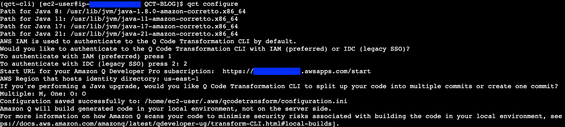
Post Syndicated from xkcd.com original https://xkcd.com/3074/
Post Syndicated from xkcd.com original https://xkcd.com/3074/
Post Syndicated from Chris McPeek original https://aws.amazon.com/blogs/compute/enriching-and-customizing-notifications-with-amazon-eventbridge-pipes/
This blog post authored by Elie Elmalem, Associate Scale Solutions Architect
When implementing event-driven architectures, customers frequently need to enrich their incoming events with additional information to make them more valuable for downstream consumers. Traditionally, customers using Amazon EventBridge would accomplish this by writing AWS Lambda functions to augment their events with supplementary data. However, this approach requires writing and maintaining custom code, adding complexity to their event processing pipeline.
Amazon EventBridge Pipes simplifies this process by providing a streamlined, managed service for event enrichment without the need to write and manage custom Lambda functions. This blog post demonstrates how you can use EventBridge Pipes’ built-in data enrichment capabilities to dynamically enhance your events with additional context and customer-specific details, making event processing more efficient and easier to maintain.
Amazon EventBridge creates a direct connection between sources and targets. Using an EventBridge bus helps you route and fan-out events to services in a pub/sub pattern. EventBridge Pipes on the other hand help you with point-to-point service integrations patterns. What sets it apart from the traditional event bus/rule pattern is its data transformation and enrichment support.
When defining an EventBridge Pipes, you specify the source and the target of the pipe. Pipes support a variety of sources and targets. Between the source and target, EventBridge Pipes supports filtering and enrichment. The filtering enables you to select and process a targeted subset of events. Enrichment allows you to enhance data by adding missing information before sending it to a target. For instance, if an event lacks necessary information, it ensures the target can properly consume the event. Enriching data can be very powerful, as it makes it possible to enhance a generic event and transform it. EventBridge Pipes support enrichment using Lambda functions, AWS Step Functions, Amazon API Gateway and EventBridge API destinations. More details about these concepts can be found in the Amazon EventBridge Pipes concepts documentation.

Figure 1: Representation of EventBridge Pipes showing filter and enrichment steps
This blog post will use the enrichment step of the pipe to create custom notifications.
To illustrate the functionality, this post uses a use case from a clothing retailer. Businesses such as this retailer want to keep their loyal customers engaged. Often, they rely on bulk promotional emails which lack personalization. In this use case, the retailer wants to send targeted promotion codes. As soon as the 10th order is placed, the code is sent via email or SMS to their customer.
Without EventBridge Pipes, this would be implemented using EventBridge to respond to the order event. All the events are sent to a custom Lambda function to process it. If the order meets the right conditions, the Lambda function sends a notification with the discount code to the customer using Amazon Simple Notification Service (Amazon SNS).

Figure 2: Traditional approach using EventBridge
While this architecture works, it requires you to maintain the integration code as well as the data enriching logic within the Lambda function as the function needs to extract the necessary information from the events and manage routing to SNS. As more microservices follow the same pattern, the code becomes more complex. This can lead to longer execution times along with higher cost and greater maintenance effort.
Amazon EventBridge Pipes can be used to simplify the previous implementation by handling the enrichment and integration between services. Amazon EventBridge Pipes take care of sending the event to your configured enrichment step and then routes the enriched event to the target. If the chosen method is a Lambda function, it leaves the function code to only focus on enrichment logic. It eliminates the need for code to extract the necessary fields from the event and to send notifications.

Figure 3: Solution architecture using EventBridge Pipes
As the event comes into the pipe, the enrichment step triggers a Lambda function, which will check eligibility and returns the message to route to SNS. If the customer is not eligible for a discount code, it returns an order confirmed message with the data retrieved from the original order event. If the customer is eligible for a discount, the message also contains the discount code.
This is the architecture for the updated flow:
To build the updated flow, I have chosen to use the AWS Cloud Development Kit (CDK) in Python. You can use the code given here to deploy it into your account. The code can also be found on GitHub.
Note: This sample code is for testing purposes only and is not intended to be used in a production account.
For this solution, you need the following prerequisites:
Once the prerequisites are met, set up a new Python CDK project in an empty directory:
Then, activate the virtual environment and install the CDK’s dependencies:
The cdk init command creates a blog_code folder. The GitHub repository contains the code for the blog_code_stack.py file inside the blog_code folder.
Then, within the blog_code folder, create a new folder called lambda. Inside this new folder, create a file called index.py. This file will contain the code for the enrichment lambda function. Once again, this code can be found in the GitHub repository. Here is a section of the Lambda code:
def lambda_handler(event, context):

    message = json.loads(event[0]['body'])

    id = message['id']
    order_content = message['order_content']

    nmb_orders = get_number_of_orders(id)

    # Calculate orders left
    orders_left = MAX_ORDERS - nmb_orders

    # Update the DynamoDB table with the new number of orders
    if nmb_orders == MAX_ORDERS:
        update_table(id, 0)
    else:
        update_table(id, nmb_orders)

    if orders_left == 0:
        return [f"Thank you for your order of {order_content}. You have earned a 10% discount code on your next order: XA5GT2SF"]
    else:
        # Return the confirmation message
        return [f"Thank you for your order of {order_content}. This is your confirmation message! Only {orders_left} orders left until a 10% discount!"]
The Lambda function works in the following way:
Now, deploy the CDK stack into your account. Make sure that you are in the root directory of your project:
Once the stack has finished deploying, you will find an EventBridge pipe visible on the console by going to the EventBridge service page and clicking on Pipes in the left panel.
To test the solution, you must first set up a subscription to the SNS topic to receive notifications. It is recommended to set up email notifications for simplicity and testing purposes. To do so, follow the instructions on the Amazon SNS documentation for the topic with name TargetTopic. When the subscription is set up, don’t forget to check your email inbox and confirm the subscription.
Once notifications are set up, visit the DynamoDB console page. You need to manually add an entry to the eligibility table to mimic a real environment:
The Items returned table should look like the following. This assumes that the customer has already place 8 orders.

Figure 4: Items returned table after adding a new item
Now, visit the SQS console page. You will need to send a message to the queue to mimic new orders being placed.
{
    "order_content": "large shirt",
    "id": "01",
    "username": "johndoe01",
    "transaction_time": "10:04:00"
  }
After a few minutes, you should receive an email confirming your order, as your order message is considered to be the 9th order. Send the message again to place a 10th order and you should receive your discount code!

Figure 5: Email received with a discount code
To delete the resources in your account, run the following command in the root directory of your project:
cdk destroy
This blog post showed how Amazon EventBridge Pipes and its enrichment feature can help you create tailored notifications. First, it discussed how it could be implemented using EventBridge and then presented a simplified implementation using EventBridge Pipes.
For more information on common patterns for EventBridge Pipes, you can check out Implementing architectural patterns with Amazon EventBridge Pipes.
For more serverless learning resources, visit Serverless Land. To find more patterns, go directly to the Serverless Patterns Collection.
Post Syndicated from Sébastien Stormacq original https://aws.amazon.com/blogs/aws/aws-announces-pixtral-large-25-02-model-in-amazon-bedrock-serverless/
Today, we announce that the Pixtral Large 25.02 model is now available in Amazon Bedrock as a fully managed, serverless offering. AWS is the first major cloud provider to deliver Pixtral Large as a fully managed, serverless model.
Working with large foundation models (FMs) often requires significant infrastructure planning, specialized expertise, and ongoing optimization to handle the computational demands effectively. Many customers find themselves managing complex environments or making trade-offs between performance and cost when deploying these sophisticated models.
The Pixtral Large model, developed by Mistral AI, represents their first multimodal model that combines advanced vision capabilities with powerful language understanding. A 128K context window makes it ideal for complex visual reasoning tasks. The model delivers exceptional performance on key benchmarks including MathVista, DocVQA, and VQAv2, demonstrating its effectiveness across document analysis, chart interpretation, and natural image understanding.
One of the most powerful aspects of Pixtral Large is its multilingual capability. The model supports dozens of languages including English, French, German, Spanish, Italian, Chinese, Japanese, Korean, Portuguese, Dutch, and Polish, making it accessible to global teams and applications. It’s also trained on more than 80 programming languages including Python, Java, C, C++, JavaScript, Bash, Swift, and Fortran, providing robust code generation and interpretation capabilities.
Developers will appreciate the model’s agent-centric design with built-in function calling and JSON output formatting, which simplifies integration with existing systems. Its strong system prompt adherence improves reliability when working with Retrieval Augmented Generation (RAG) applications and large context scenarios.
With Pixtral Large in Amazon Bedrock, you can now access this advanced model without having to provision or manage any infrastructure. The serverless approach lets you scale usage based on actual demand without upfront commitments or capacity planning. You pay only for what you use, with no idle resources.
Cross-Region inference
Pixtral Large is now available in Amazon Bedrock across multiple AWS Regions through cross-Region inference.
With Amazon Bedrock cross-Region inference, you can access a single FM across multiple geographic Regions while maintaining high availability and low latency for global applications. For example, when a model is deployed in both European and US Regions, you can access it through Region-specific API endpoints using distinct prefixes: eu.model-id for European Regions and us.model-id for US Regions . This approach enables Amazon Bedrock to route inference requests to the geographically closest endpoint, reducing latency while helping to meet regulatory compliance by keeping data processing within desired geographic boundaries. The system automatically handles traffic routing and load balancing across these Regional deployments, providing seamless scalability and redundancy without requiring you to keep track of individual Regions where the model is actually deployed.
See it in action
As a developer advocate, I’m constantly exploring how our newest capabilities can solve real problems. Recently, I had a perfect opportunity to test the new multimodal capabilities in the Amazon Bedrock Converse API when my daughter asked for help with her physics exam preparation.
Last weekend, my kitchen table was covered with practice exams full of complex diagrams, force vectors, and equations. My daughter was struggling with conceptualizing how to approach these problems. That’s when I realized this was the perfect use case for the multimodal capabilities we’d just launched. I snapped photos of a particularly challenging problem sheet containing several graphs and mathematical notation, then used the Converse API to create a simple application that could analyze the images. Together, we uploaded the physics exam materials and asked the model to explain the solution approach.

What happened next impressed both of us—the model interpreted the diagrams, recognized the french language and the mathematical notation, and provided a step-by-step explanation of how to solve each problem. As we asked follow-up questions about specific concepts, the model maintained context across our entire conversation, creating a tutoring experience that felt remarkably natural.
# Effet Doppler avec une Source Sonore en Rotation

## Analyse du problème

Ce problème concerne l'effet Doppler produit par une source sonore en rotation. Une source émettant un son à 1500 Hz tourne sur une table tournante dans le sens antihoraire, et nous devons déterminer comment les fréquences sont perçues par un microphone fixe.

## Concepts clés

L'effet Doppler se produit lorsqu'il y a un mouvement relatif entre une source sonore et un observateur. La fréquence perçue dépend de si la source se rapproche ou s'éloigne de l'observateur.

La formule de l'effet Doppler est:
- Pour une source qui se rapproche: $f_{observée} = f_{source} \cdot \frac{v_{son}}{v_{son} - v_{source}}$
- Pour une source qui s'éloigne: $f_{observée} = f_{source} \cdot \frac{v_{son}}{v_{son} + v_{source}}$

## Solution étape par étape

### Étape 1: Analyser le mouvement de la source
La source tourne sur un cercle et le microphone est fixe à 40 cm du centre de rotation. Aux différentes positions (a, b, c), la source a des vitesses radiales différentes par rapport au microphone:

- Position a: La source se déplace perpendiculairement à la ligne source-microphone (vitesse radiale nulle)
- Position b: La source s'éloigne du microphone (vitesse radiale positive)
- Position c: La source se rapproche du microphone (vitesse radiale négative)

### Étape 2: Déterminer l'effet sur les fréquences perçues

- À la position a: Pas d'effet Doppler car la vitesse radiale est nulle, donc $f_a = f_{source} = 1500$ Hz
- À la position b: La source s'éloigne, donc $f_b < f_{source}$, donc $f_b < 1500$ Hz
- À la position c: La source se rapproche, donc $f_c > f_{source}$, donc $f_c > 1500$ Hz

### Étape 3: Comparer les fréquences

D'après notre analyse:
- $f_a = 1500$ Hz
- $f_b < 1500$ Hz
- $f_c > 1500$ Hz

Donc: $f_c > f_a > f_b$

## Conclusion

La proposition correcte est: $f_c > f_a > f_b$

Cette réponse correspond à la troisième proposition dans l'énoncé. Lorsque la source tourne, la fréquence perçue est plus élevée quand la source se rapproche (position c), égale à la fréquence émise quand la source se déplace perpendiculairement (position a), et plus basse quand la source s'éloigne (position b).
The model uses the language of the question to respond. After a thoughtful analysis, it says that the correct answer is f_c > f_a > f_b (and it is right!)
The beauty of this interaction was how seamlessly the Converse API handled the multimodal inputs. As a builder, I didn’t need to worry about the complexity of processing images alongside text—the API managed that complexity and returned structured responses that my simple application could present directly to my daughter.
Here is the code I wrote. I used the Swift programming language, just to show that Python is not the only option you have  .
.
private let modelId = "us.mistral.pixtral-large-2502-v1:0"

// Define the system prompt that instructs Claude how to respond
let systemPrompt = """
You are a math and physics tutor. Your task is to:
1. Read and understand the math or physics problem in the image
2. Provide a clear, step-by-step solution to the problem
3. Briefly explain any relevant concepts used in solving the problem
4. Be precise and accurate in your calculations
5. Use mathematical notation when appropriate

Format your response with clear section headings and numbered steps.
"""
let system: BedrockRuntimeClientTypes.SystemContentBlock = .text(systemPrompt)

// Create the user message with text prompt and image
let userPrompt = "Please solve this math or physics problem. Show all steps and explain the concepts involved."
let prompt: BedrockRuntimeClientTypes.ContentBlock = .text(userPrompt)
let image: BedrockRuntimeClientTypes.ContentBlock = .image(.init(format: .jpeg, source: .bytes(finalImageData)))

// Create the user message with both text and image content
let userMessage = BedrockRuntimeClientTypes.Message(
    content: [prompt, image],
    role: .user
)

// Initialize the messages array with the user message
var messages: [BedrockRuntimeClientTypes.Message] = []
messages.append(userMessage)

// Configure the inference parameters
let inferenceConfig: BedrockRuntimeClientTypes.InferenceConfiguration = .init(maxTokens: 4096, temperature: 0.0)

// Create the input for the Converse API with streaming
let input = ConverseStreamInput(inferenceConfig: inferenceConfig, messages: messages, modelId: modelId, system: [system])

// Make the streaming request
do {
    // Process the stream
    let response = try await bedrockClient.converseStream(input: input)

    // Iterate through the stream events
    for try await event in stream {
        switch event {
        case .messagestart:
            print("AI-assistant started to stream")

        case let .contentblockdelta(deltaEvent):
            // Handle text content as it arrives
            if case let .text(text) = deltaEvent.delta {
                DispatchQueue.main.async {
                    self.streamedResponse += text
                }
            }

        case .messagestop:
            print("Stream ended")
            // Create a complete assistant message from the streamed response
            let assistantMessage = BedrockRuntimeClientTypes.Message(
                content: [.text(self.streamedResponse)],
                role: .assistant
            )
            messages.append(assistantMessage)

        default:
            break
        }
    }
And the result in the app is stunning.

By the time her exam rolled around, she felt confident and prepared—and I had a compelling real-world example of how our multimodal capabilities in Amazon Bedrock can create meaningful experiences for users.
Get started today
The new model is available through these Regional API endpoints: US East (Ohio, N. Virginia), US West (Oregon), and Europe (Frankfurt, Ireland, Paris, Stockholm). This Regional availability helps you meet data residency requirements while minimizing latency.
You can start using the model through either the AWS Management Console or programmatically through the AWS Command Line Interface (AWS CLI) and AWS SDK using the model ID mistral.pixtral-large-2502-v1:0.
This launch represents a significant step forward in making advanced multimodal AI accessible to developers and organizations of all sizes. By combining Mistral AI’s cutting-edge model with AWS serverless infrastructure, you can now focus on building innovative applications without worrying about the underlying complexity.
Visit the Amazon Bedrock console today to start experimenting with Pixtral Large 25.02 and discover how it can enhance your AI-powered applications.
How is the News Blog doing? Take this 1 minute survey!
(This survey is hosted by an external company. AWS handles your information as described in the AWS Privacy Notice. AWS will own the data gathered via this survey and will not share the information collected with survey respondents.)
Post Syndicated from Danilo Poccia original https://aws.amazon.com/blogs/aws/introducing-amazon-nova-sonic-human-like-voice-conversations-for-generative-ai-applications/
Voice interfaces are essential to enhance customer experience in different areas such as customer support call automation, gaming, interactive education, and language learning. However, there are challenges when building voice-enabled applications.
Traditional approaches in building voice-enabled applications require complex orchestration of multiple models, such as speech recognition to convert speech to text, language models to understand and generate responses, and text-to-speech to convert text back to audio.
This fragmented approach not only increases development complexity but also fails to preserve crucial linguistic context such as tone, prosody, and speaking style that are essential for natural conversations. This can affect conversational AI applications that need low latency and nuanced understanding of verbal and non-verbal cues for fluid dialog handling and natural turn-taking.
To streamline the implementation of speech-enabled applications, today we are introducing Amazon Nova Sonic, the newest addition to the Amazon Nova family of foundation models (FMs) available in Amazon Bedrock.
Amazon Nova Sonic unifies speech understanding and generation into a single model that developers can use to create natural, human-like conversational AI experiences with low latency and industry-leading price performance. This integrated approach streamlines development and reduces complexity when building conversational applications.
Its unified model architecture delivers expressive speech generation and real-time text transcription without requiring a separate model. The result is an adaptive speech response that dynamically adjusts its delivery based on prosody, such as pace and timbre, of input speech.
When using Amazon Nova Sonic, developers have access to function calling (also known as tool use) and agentic workflows to interact with external services and APIs and perform tasks in the customer’s environment, including knowledge grounding with enterprise data using Retrieval-Augmented Generation.
At launch, Amazon Nova Sonic provides robust speech understanding for American and British English across various speaking styles and acoustic conditions, with additional languages coming soon.
Amazon Nova Sonic is developed with responsible AI at the forefront of innovation, featuring built-in protections for content moderation and watermarking.
Amazon Nova Sonic in action
The scenario for this demo is a contact center in the telecommunication industry. A customer reaches out to improve their subscription plan, and Amazon Nova Sonic handles the conversation.
With tool use, the model can interact with other systems and use agentic RAG with Amazon Bedrock Knowledge Bases to gather updated, customer-specific information such as account details, subscription plans, and pricing info.
The demo shows streaming transcription of speech input and displays streaming speech responses as text. The sentiment of the conversation is displayed in two ways: a time chart illustrating how it evolves, and a pie chart representing the overall distribution. There’s also an AI insights section providing contextual tips for a call center agent. Other interesting metrics shown in the web interface are the overall talk time distribution between the customer and the agent, and the average response time.
During the conversation with the support agent, you can observe through the metrics and hear in the voices how customer sentiment improves.
The video includes an example of how Amazon Nova Sonic handles interruptions smoothly, stopping to listen and then continuing the conversation in a natural way.
Now, let’s explore how you can integrate voice capabilities in your applications.
Using Amazon Nova Sonic
To get started with Amazon Nova Sonic, you first need to toggle model access in the Amazon Bedrock console, similar to how you would enable other FMs. Navigate to the Model access section of the navigation pane, find Amazon Nova Sonic under the Amazon models, and enable it for your account.
Amazon Bedrock provides a new bidirectional streaming API (InvokeModelWithBidirectionalStream) to help you implement real-time, low-latency conversational experiences on top of the HTTP/2 protocol. With this API, you can stream audio input to the model and receive audio output in real time, so that the conversation flows naturally.
You can use Amazon Nova Sonic with the new API with this model ID: amazon.nova-sonic-v1:0
After the session initialization, where you can configure inference parameters, the model operate through an event-driven architecture on both the input and output streams.
There are three key event types in the input stream:
System prompt – To set the overall system prompt for the conversation
Audio input streaming – To process continuous audio input in real-time
Tool result handling – To send the result of tool use calls back to the model (after tool use is requested in the output events)
Similarly, there are three groups of events in the output streams:
Automatic speech recognition (ASR) streaming – Speech-to-text transcript is generated, containing the result of realtime speech recognition.
Tool use handling – If there are a tool use events, they need to be handled using the information provided here, and the results sent back as input events.
Audio output streaming – To play output audio in real-time, a buffer is needed, because Amazon Nova Sonic model generates audio faster than real-time playback.
You can find examples of using Amazon Nova Sonic in the Amazon Nova model cookbook repository.
Prompt engineering for speech
When crafting prompts for Amazon Nova Sonic, your prompts should optimize content for auditory comprehension rather than visual reading, focusing on conversational flow and clarity when heard rather than seen.
When defining roles for your assistant, focus on conversational attributes (such as warm, patient, concise) rather than text-oriented attributes (detailed, comprehensive, systematic). A good baseline system prompt might be:
You are a friend. The user and you will engage in a spoken dialog exchanging the transcripts of a natural real-time conversation. Keep your responses short, generally two or three sentences for chatty scenarios.
More generally, when creating prompts for speech models, avoid requesting visual formatting (such as bullet points, tables, or code blocks), voice characteristic modifications (accent, age, or singing), or sound effects.
Things to know
Amazon Nova Sonic is available today in the US East (N. Virginia) AWS Region. Visit Amazon Bedrock pricing to see the pricing models.
Amazon Nova Sonic can understand speech in different speaking styles and generates speech in expressive voices, including both masculine-sounding and feminine-sounding voices, in different English accents, including American and British. Support for additional languages will be coming soon.
Amazon Nova Sonic handles user interruptions gracefully without dropping the conversational context and is robust to background noise. The model supports a context window of 32K tokens for audio with a rolling window to handle longer conversations and has a default session limit of 8 minutes.
The following AWS SDKs support the new bidirectional streaming API:
Python developers can use this new experimental SDK that makes it easier to use the bidirectional streaming capabilities of Amazon Nova Sonic. We’re working to add support to the other AWS SDKs.
I’d like to thank Reilly Manton and Chad Hendren, who set up the demo with the contact center in the telecommunication industry, and Anuj Jauhari, who helped me understand the rich landscape in which speech-to-speech models are being deployed.
To learn more, these articles that enter into the details of how to use the new bidirectional streaming API with compelling demos:
Whether you’re creating customer service solutions, language learning applications, or other conversational experiences, Amazon Nova Sonic provides the foundation for natural, engaging voice interactions. To get started, visit the Amazon Bedrock console today. To learn more, visit the Amazon Nova section of the user guide.
– Danilo
How is the News Blog doing? Take this 1 minute survey!
(This survey is hosted by an external company. AWS handles your information as described in the AWS Privacy Notice. AWS will own the data gathered via this survey and will not share the information collected with survey respondents.)
Post Syndicated from Adam Barnett original https://blog.rapid7.com/2025/04/08/patch-tuesday-april-2025/

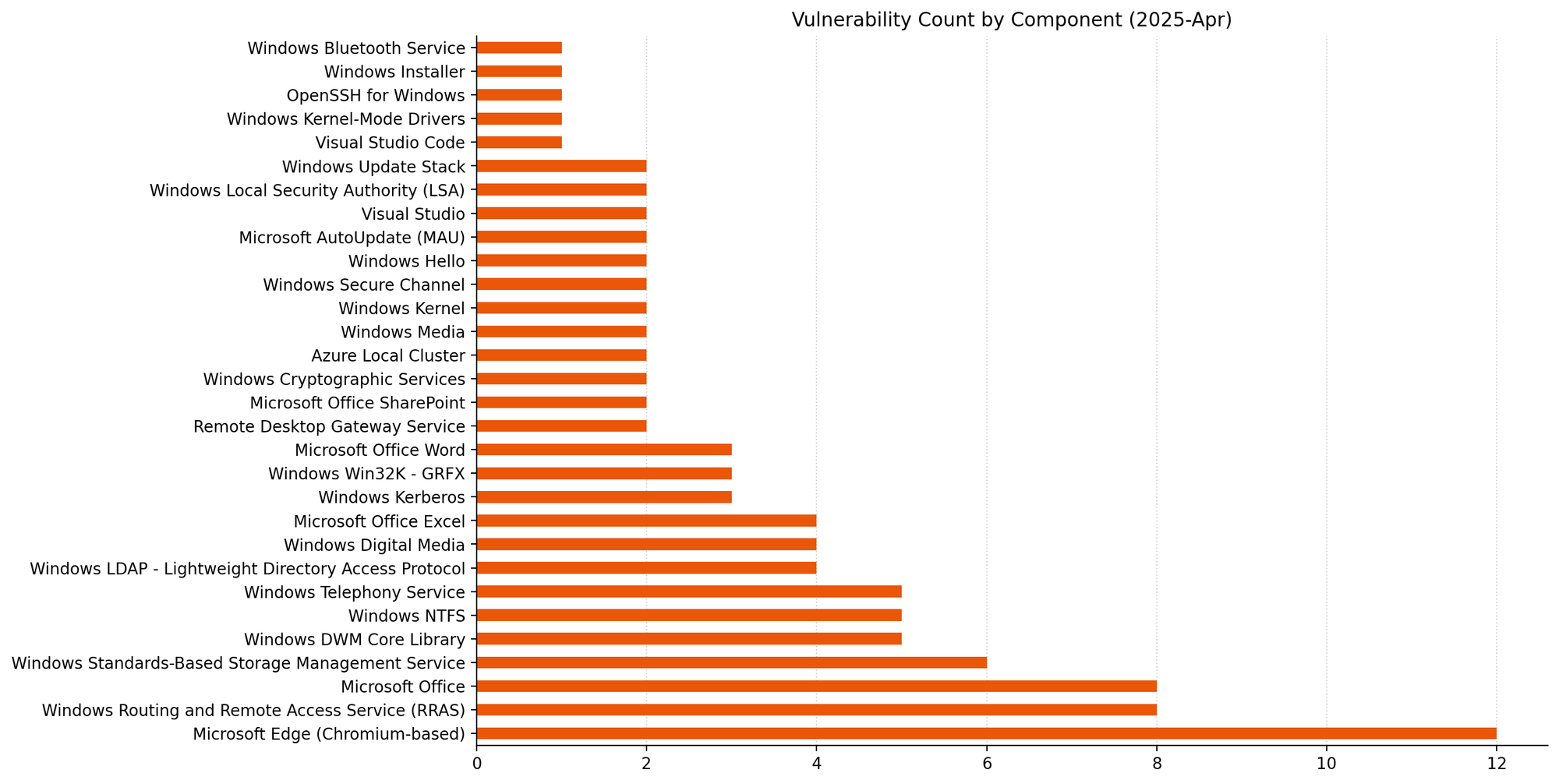
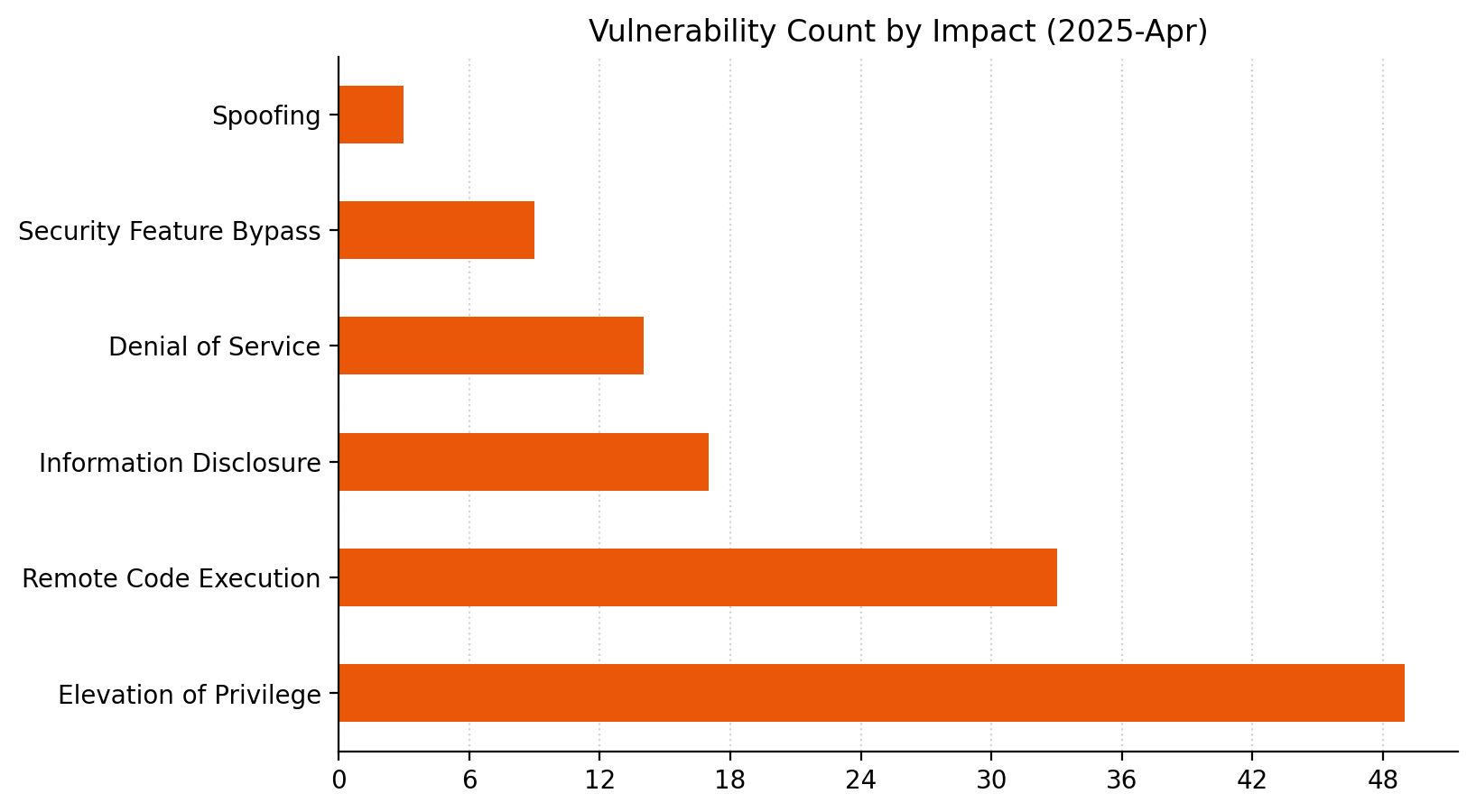
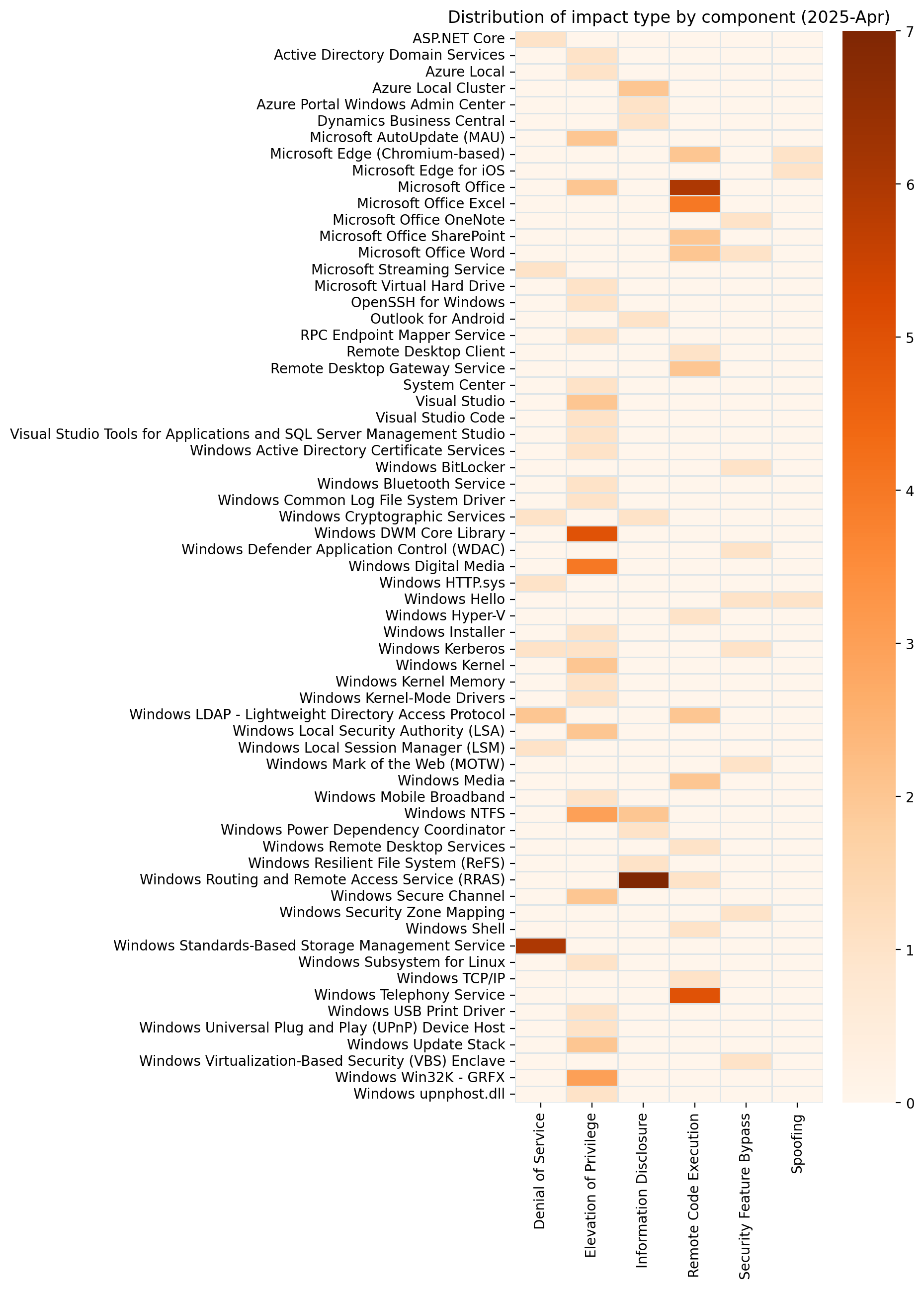
Microsoft is addressing 121 vulnerabilities this April 2025 Patch Tuesday, which is more than twice as many as last month. Microsoft has evidence of in-the-wild exploitation for just one of the vulnerabilities published today, which is already reflected in CISA KEV. Once again, Microsoft has published zero-day vulnerabilities on Patch Tuesday without evaluating any of them as critical severity at time of publication, so that’s now a seven month unbroken streak. Today also sees the publication of 11 critical remote code execution (RCE) vulnerabilities. 13 browser vulnerabilities have already been published separately this month, and are not included in the total.
The Windows Common Log File System (CLFS) Driver is firmly back on our radar today with CVE-2025-29824, a zero-day local elevation of privilege vulnerability. First, the good news: the Acknowledgements section credits the Microsoft Threat Intelligence Center, so the exploit was successfully reproduced by Microsoft; the less-good news is that someone other than Microsoft was first to discover the exploit, because otherwise Microsoft wouldn’t be listing CVE-2025-29824 as exploited in the wild. The advisory does not specify what privilege level is achieved upon successful exploitation, but it’ll be SYSTEM, because that’s the prize for all the other CLFS elevation of privilege zero-day vulnerabilities. As usual, some form of less-privileged local access is a pre-requisite, but attack complexity is low, so this is the sort of vulnerability which goes into any standard break-and-enter toolkit. Given the long history of similar vulnerabilities, it would be more surprising if exploit code wasn’t publicly available in the not-too-distant future. Although December 2024 Patch Tuesday seems as though it must have been a very long time ago, any standard calendar will tell us that only 119 days have elapsed since the last zero-day CLFS local elevation of privilege. Rapid7 discussed the history of CLFS zero-day elevation of privilege vulnerabilities at the time. All versions of Windows receive a patch, except for the venerable LTSC Windows 10 1507, which is listed on the advisory as vulnerable, but left out in the cold with no update; the FAQ says to check back later. Windows 10 LTSC 1507 is scheduled for end of servicing on 2025-10-14, so the clock is ticking regardless.
Although it has been many months since we’ve seen a critical zero-day vulnerability from Microsoft, there is no shortage of critical remote code execution (RCE) vulnerabilities published today. Defenders responsible for an LDAP server — which means almost any organization with a non-trivial Microsoft footprint — should add patching for CVE-2025-26663 to their to-do list. With no privileges required, no need for user interaction, and code execution presumably in the context of the LDAP server itself, successful exploitation would be an attractive shortcut to any attacker. Anyone wondering if today is a re-run of December 2024 Patch Tuesday can take some small solace in the fact that the worst of the trio of LDAP critical RCEs published at the end of last year was likely easier to exploit than today’s example, since today’s CVE-2025-26663 requires that an attacker win a race condition. Despite that, Microsoft still expects that exploitation is more likely.
If you breathe a sigh of relief when you see LDAP server critical RCE vulnerabilities like CVE-2025-26663, because you’re certain that you don’t have any Windows LDAP servers in your estate, how about LDAP clients? CVE-2025-26670 describes a critical RCE in the LDAP client, although the FAQ confusingly states that exploitation would require an attacker to “send specially crafted requests to a vulnerable LDAP server”; this seems like it might be a data entry error on the advisory FAQ, so keep an eye out for an update to that section of the advisory. Assuming the rest of the advisory is all present and correct, exploitation requires that the attacker win a race condition, which keeps the attack complexity higher than it otherwise would be. While we wait for clarification, it’s still a critical RCE which Microsoft rates as “exploitation more likely”. On that basis, patching is always recommended.
The prolific Windows vulnerability pioneers at Kunlun Lab are credited with a pair of critical RCE vulnerabilities in Windows Remote Desktop Services. Although both CVE-2025-27480 and CVE-2025-27482 share a CVSSv3 base score of 8.1, Microsoft has ranked them both as critical using its own proprietary severity ranking scale. Both vulnerabilities require that an attacker win a race condition. If you’ve ever read Microsoft’s guide to deploying the Remote Desktop Gateway role, you probably have some systems to patch.
Some Microsoft security advisory FAQs provide a satisfying level of detail, whereas others raise more questions than they answer. CVE-2025-27491 is a Hyper-V critical RCE which falls into the second category, since it states that an attacker must be authenticated — no need for elevated privileges — but also that the attacker must send the user a malicious site and convince them to open it, and it’s not at all clear why authentication would be required in that case. Also unusual: the remediation table on the advisory lists several 32-bit versions of Windows as receiving patches, although Hyper-V requires a 64-bit processor and a 64-bit host OS.
In Microsoft product lifecycle news, Dynamics GP 2015 moves past the end of extended support today. The next batch of significant lifecycle status changes are due in July 2025, when SQL Server 2012 ESU program draws to a close.
| CVE | Title | Exploited? | Publicly disclosed? | CVSSv3 base score |
|---|---|---|---|---|
| CVE-2025-29805 | Outlook for Android Information Disclosure Vulnerability | No | No | 7.5 |
| CVE | Title | Exploited? | Publicly disclosed? | CVSSv3 base score |
|---|---|---|---|---|
| CVE-2025-27489 | Azure Local Elevation of Privilege Vulnerability | No | No | 7.8 |
| CVE-2025-26628 | Azure Local Cluster Information Disclosure Vulnerability | No | No | 7.3 |
| CVE-2025-25002 | Azure Local Cluster Information Disclosure Vulnerability | No | No | 6.8 |
| CVE | Title | Exploited? | Publicly disclosed? | CVSSv3 base score |
|---|---|---|---|---|
| CVE-2025-25000 | Microsoft Edge (Chromium-based) Remote Code Execution Vulnerability | No | No | 8.8 |
| CVE-2025-29815 | Microsoft Edge (Chromium-based) Remote Code Execution Vulnerability | No | No | 7.6 |
| CVE-2025-29796 | Microsoft Edge for iOS Spoofing Vulnerability | No | No | 4.7 |
| CVE-2025-25001 | Microsoft Edge for iOS Spoofing Vulnerability | No | No | 4.3 |
| CVE-2025-3074 | Chromium: CVE-2025-3074 Inappropriate implementation in Downloads | No | No | N/A |
| CVE-2025-3073 | Chromium: CVE-2025-3073 Inappropriate implementation in Autofill | No | No | N/A |
| CVE-2025-3072 | Chromium: CVE-2025-3072 Inappropriate implementation in Custom Tabs | No | No | N/A |
| CVE-2025-3071 | Chromium: CVE-2025-3071 Inappropriate implementation in Navigations | No | No | N/A |
| CVE-2025-3070 | Chromium: CVE-2025-3070 Insufficient validation of untrusted input in Extensions | No | No | N/A |
| CVE-2025-3069 | Chromium: CVE-2025-3069 Inappropriate implementation in Extensions | No | No | N/A |
| CVE-2025-3068 | Chromium: CVE-2025-3068 Inappropriate implementation in Intents | No | No | N/A |
| CVE-2025-3067 | Chromium: CVE-2025-3067 Inappropriate implementation in Custom Tabs | No | No | N/A |
| CVE-2025-3066 | Chromium: CVE-2025-3066 Use after free in Navigations | No | No | N/A |
| CVE | Title | Exploited? | Publicly disclosed? | CVSSv3 base score |
|---|---|---|---|---|
| CVE-2025-26682 | ASP.NET Core and Visual Studio Denial of Service Vulnerability | No | No | 7.5 |
| CVE-2025-29802 | Visual Studio Elevation of Privilege Vulnerability | No | No | 7.3 |
| CVE-2025-29804 | Visual Studio Elevation of Privilege Vulnerability | No | No | 7.3 |
| CVE-2025-20570 | Visual Studio Code Elevation of Privilege Vulnerability | No | No | 6.8 |
| CVE | Title | Exploited? | Publicly disclosed? | CVSSv3 base score |
|---|---|---|---|---|
| CVE-2025-29803 | Visual Studio Tools for Applications and SQL Server Management Studio Elevation of Privilege Vulnerability | No | No | 7.3 |
| CVE | Title | Exploited? | Publicly disclosed? | CVSSv3 base score |
|---|---|---|---|---|
| CVE-2025-29821 | Microsoft Dynamics Business Central Information Disclosure Vulnerability | No | No | 5.5 |
| CVE | Title | Exploited? | Publicly disclosed? | CVSSv3 base score |
|---|---|---|---|---|
| CVE-2025-29794 | Microsoft SharePoint Remote Code Execution Vulnerability | No | No | 8.8 |
| CVE-2025-27747 | Microsoft Word Remote Code Execution Vulnerability | No | No | 7.8 |
| CVE-2025-29820 | Microsoft Word Remote Code Execution Vulnerability | No | No | 7.8 |
| CVE-2025-29822 | Microsoft OneNote Security Feature Bypass Vulnerability | No | No | 7.8 |
| CVE-2025-27745 | Microsoft Office Remote Code Execution Vulnerability | No | No | 7.8 |
| CVE-2025-27748 | Microsoft Office Remote Code Execution Vulnerability | No | No | 7.8 |
| CVE-2025-27749 | Microsoft Office Remote Code Execution Vulnerability | No | No | 7.8 |
| CVE-2025-27746 | Microsoft Office Remote Code Execution Vulnerability | No | No | 7.8 |
| CVE-2025-26642 | Microsoft Office Remote Code Execution Vulnerability | No | No | 7.8 |
| CVE-2025-27744 | Microsoft Office Elevation of Privilege Vulnerability | No | No | 7.8 |
| CVE-2025-27752 | Microsoft Excel Remote Code Execution Vulnerability | No | No | 7.8 |
| CVE-2025-29791 | Microsoft Excel Remote Code Execution Vulnerability | No | No | 7.8 |
| CVE-2025-27751 | Microsoft Excel Remote Code Execution Vulnerability | No | No | 7.8 |
| CVE-2025-27750 | Microsoft Excel Remote Code Execution Vulnerability | No | No | 7.8 |
| CVE-2025-29823 | Microsoft Excel Remote Code Execution Vulnerability | No | No | 7.8 |
| CVE-2025-29800 | Microsoft AutoUpdate (MAU) Elevation of Privilege Vulnerability | No | No | 7.8 |
| CVE-2025-29801 | Microsoft AutoUpdate (MAU) Elevation of Privilege Vulnerability | No | No | 7.8 |
| CVE-2025-29816 | Microsoft Word Security Feature Bypass Vulnerability | No | No | 7.5 |
| CVE-2025-29792 | Microsoft Office Elevation of Privilege Vulnerability | No | No | 7.3 |
| CVE-2025-29793 | Microsoft SharePoint Remote Code Execution Vulnerability | No | No | 7.2 |
| CVE | Title | Exploited? | Publicly disclosed? | CVSSv3 base score |
|---|---|---|---|---|
| CVE-2025-27743 | Microsoft System Center Elevation of Privilege Vulnerability | No | No | 7.8 |
| CVE | Title | Exploited? | Publicly disclosed? | CVSSv3 base score |
|---|---|---|---|---|
| CVE-2025-26678 | Windows Defender Application Control Security Feature Bypass Vulnerability | No | No | 8.4 |
| CVE-2025-27482 | Windows Remote Desktop Services Remote Code Execution Vulnerability | No | No | 8.1 |
| CVE-2025-26639 | Windows USB Print Driver Elevation of Privilege Vulnerability | No | No | 7.8 |
| CVE-2025-26675 | Windows Subsystem for Linux Elevation of Privilege Vulnerability | No | No | 7.8 |
| CVE-2025-27729 | Windows Shell Remote Code Execution Vulnerability | No | No | 7.8 |
| CVE-2025-29811 | Windows Mobile Broadband Driver Elevation of Privilege Vulnerability | No | No | 7.8 |
| CVE-2025-26666 | Windows Media Remote Code Execution Vulnerability | No | No | 7.8 |
| CVE-2025-26674 | Windows Media Remote Code Execution Vulnerability | No | No | 7.8 |
| CVE-2025-27728 | Windows Kernel-Mode Driver Elevation of Privilege Vulnerability | No | No | 7.8 |
| CVE-2025-27739 | Windows Kernel Elevation of Privilege Vulnerability | No | No | 7.8 |
| CVE-2025-27476 | Windows Digital Media Elevation of Privilege Vulnerability | No | No | 7.8 |
| CVE-2025-27467 | Windows Digital Media Elevation of Privilege Vulnerability | No | No | 7.8 |
| CVE-2025-27730 | Windows Digital Media Elevation of Privilege Vulnerability | No | No | 7.8 |
| CVE-2025-24058 | Windows DWM Core Library Elevation of Privilege Vulnerability | No | No | 7.8 |
| CVE-2025-27490 | Windows Bluetooth Service Elevation of Privilege Vulnerability | No | No | 7.8 |
| CVE-2025-27731 | Microsoft OpenSSH for Windows Elevation of Privilege Vulnerability | No | No | 7.8 |
| CVE-2025-24074 | Microsoft DWM Core Library Elevation of Privilege Vulnerability | No | No | 7.8 |
| CVE-2025-24073 | Microsoft DWM Core Library Elevation of Privilege Vulnerability | No | No | 7.8 |
| CVE-2025-24060 | Microsoft DWM Core Library Elevation of Privilege Vulnerability | No | No | 7.8 |
| CVE-2025-24062 | Microsoft DWM Core Library Elevation of Privilege Vulnerability | No | No | 7.8 |
| CVE-2025-29812 | DirectX Graphics Kernel Elevation of Privilege Vulnerability | No | No | 7.8 |
| CVE-2025-29809 | Windows Kerberos Security Feature Bypass Vulnerability | No | No | 7.1 |
| CVE-2025-27491 | Windows Hyper-V Remote Code Execution Vulnerability | No | No | 7.1 |
| CVE-2025-27475 | Windows Update Stack Elevation of Privilege Vulnerability | No | No | 7 |
| CVE-2025-26649 | Windows Secure Channel Elevation of Privilege Vulnerability | No | No | 7 |
| CVE-2025-27492 | Windows Secure Channel Elevation of Privilege Vulnerability | No | No | 7 |
| CVE-2025-26640 | Windows Digital Media Elevation of Privilege Vulnerability | No | No | 7 |
| CVE-2025-26681 | Win32k Elevation of Privilege Vulnerability | No | No | 6.7 |
| CVE-2025-26651 | Windows Local Session Manager (LSM) Denial of Service Vulnerability | No | No | 6.5 |
| CVE-2025-26635 | Windows Hello Security Feature Bypass Vulnerability | No | No | 6.5 |
| CVE-2025-27735 | Windows Virtualization-Based Security (VBS) Security Feature Bypass Vulnerability | No | No | 6 |
| CVE-2025-27736 | Windows Power Dependency Coordinator Information Disclosure Vulnerability | No | No | 5.5 |
| CVE-2025-29808 | Windows Cryptographic Services Information Disclosure Vulnerability | No | No | 5.5 |
| CVE-2025-26644 | Windows Hello Spoofing Vulnerability | No | No | 5.1 |
| CVE | Title | Exploited? | Publicly disclosed? | CVSSv3 base score |
|---|---|---|---|---|
| CVE-2025-29819 | Windows Admin Center in Azure Portal Information Disclosure Vulnerability | No | No | 6.2 |
| CVE | Title | Exploited? | Publicly disclosed? | CVSSv3 base score |
|---|---|---|---|---|
| CVE-2025-27477 | Windows Telephony Service Remote Code Execution Vulnerability | No | No | 8.8 |
| CVE-2025-21205 | Windows Telephony Service Remote Code Execution Vulnerability | No | No | 8.8 |
| CVE-2025-21221 | Windows Telephony Service Remote Code Execution Vulnerability | No | No | 8.8 |
| CVE-2025-21222 | Windows Telephony Service Remote Code Execution Vulnerability | No | No | 8.8 |
| CVE-2025-27481 | Windows Telephony Service Remote Code Execution Vulnerability | No | No | 8.8 |
| CVE-2025-26669 | Windows Routing and Remote Access Service (RRAS) Information Disclosure Vulnerability | No | No | 8.8 |
| CVE-2025-27740 | Active Directory Certificate Services Elevation of Privilege Vulnerability | No | No | 8.8 |
| CVE-2025-27737 | Windows Security Zone Mapping Security Feature Bypass Vulnerability | No | No | 8.6 |
| CVE-2025-27480 | Windows Remote Desktop Services Remote Code Execution Vulnerability | No | No | 8.1 |
| CVE-2025-26671 | Windows Remote Desktop Services Remote Code Execution Vulnerability | No | No | 8.1 |
| CVE-2025-26663 | Windows Lightweight Directory Access Protocol (LDAP) Remote Code Execution Vulnerability | No | No | 8.1 |
| CVE-2025-26647 | Windows Kerberos Elevation of Privilege Vulnerability | No | No | 8.1 |
| CVE-2025-26670 | Lightweight Directory Access Protocol (LDAP) Client Remote Code Execution Vulnerability | No | No | 8.1 |
| CVE-2025-27487 | Remote Desktop Client Remote Code Execution Vulnerability | No | No | 8 |
| CVE-2025-21204 | Windows Process Activation Elevation of Privilege Vulnerability | No | No | 7.8 |
| CVE-2025-26648 | Windows Kernel Elevation of Privilege Vulnerability | No | No | 7.8 |
| CVE-2025-27727 | Windows Installer Elevation of Privilege Vulnerability | No | No | 7.8 |
| CVE-2025-29824 | Windows Common Log File System Driver Elevation of Privilege Vulnerability | Yes | No | 7.8 |
| CVE-2025-26679 | RPC Endpoint Mapper Service Elevation of Privilege Vulnerability | No | No | 7.8 |
| CVE-2025-27741 | NTFS Elevation of Privilege Vulnerability | No | No | 7.8 |
| CVE-2025-27483 | NTFS Elevation of Privilege Vulnerability | No | No | 7.8 |
| CVE-2025-27733 | NTFS Elevation of Privilege Vulnerability | No | No | 7.8 |
| CVE-2025-26688 | Microsoft Virtual Hard Disk Elevation of Privilege Vulnerability | No | No | 7.8 |
| CVE-2025-27484 | Windows Universal Plug and Play (UPnP) Device Host Elevation of Privilege Vulnerability | No | No | 7.5 |
| CVE-2025-26686 | Windows TCP/IP Remote Code Execution Vulnerability | No | No | 7.5 |
| CVE-2025-26680 | Windows Standards-Based Storage Management Service Denial of Service Vulnerability | No | No | 7.5 |
| CVE-2025-27470 | Windows Standards-Based Storage Management Service Denial of Service Vulnerability | No | No | 7.5 |
| CVE-2025-21174 | Windows Standards-Based Storage Management Service Denial of Service Vulnerability | No | No | 7.5 |
| CVE-2025-26652 | Windows Standards-Based Storage Management Service Denial of Service Vulnerability | No | No | 7.5 |
| CVE-2025-27485 | Windows Standards-Based Storage Management Service Denial of Service Vulnerability | No | No | 7.5 |
| CVE-2025-27486 | Windows Standards-Based Storage Management Service Denial of Service Vulnerability | No | No | 7.5 |
| CVE-2025-26668 | Windows Routing and Remote Access Service (RRAS) Remote Code Execution Vulnerability | No | No | 7.5 |
| CVE-2025-26673 | Windows Lightweight Directory Access Protocol (LDAP) Denial of Service Vulnerability | No | No | 7.5 |
| CVE-2025-27469 | Windows Lightweight Directory Access Protocol (LDAP) Denial of Service Vulnerability | No | No | 7.5 |
| CVE-2025-26641 | Microsoft Message Queuing (MSMQ) Denial of Service Vulnerability | No | No | 7.5 |
| CVE-2025-27479 | Kerberos Key Distribution Proxy Service Denial of Service Vulnerability | No | No | 7.5 |
| CVE-2025-27473 | HTTP.sys Denial of Service Vulnerability | No | No | 7.5 |
| CVE-2025-29810 | Active Directory Domain Services Elevation of Privilege Vulnerability | No | No | 7.5 |
| CVE-2025-26665 | Windows upnphost.dll Elevation of Privilege Vulnerability | No | No | 7 |
| CVE-2025-27478 | Windows Local Security Authority (LSA) Elevation of Privilege Vulnerability | No | No | 7 |
| CVE-2025-21191 | Windows Local Security Authority (LSA) Elevation of Privilege Vulnerability | No | No | 7 |
| CVE-2025-27732 | Windows Graphics Component Elevation of Privilege Vulnerability | No | No | 7 |
| CVE-2025-26637 | BitLocker Security Feature Bypass Vulnerability | No | No | 6.8 |
| CVE-2025-26664 | Windows Routing and Remote Access Service (RRAS) Information Disclosure Vulnerability | No | No | 6.5 |
| CVE-2025-26667 | Windows Routing and Remote Access Service (RRAS) Information Disclosure Vulnerability | No | No | 6.5 |
| CVE-2025-27474 | Windows Routing and Remote Access Service (RRAS) Information Disclosure Vulnerability | No | No | 6.5 |
| CVE-2025-21203 | Windows Routing and Remote Access Service (RRAS) Information Disclosure Vulnerability | No | No | 6.5 |
| CVE-2025-26672 | Windows Routing and Remote Access Service (RRAS) Information Disclosure Vulnerability | No | No | 6.5 |
| CVE-2025-26676 | Windows Routing and Remote Access Service (RRAS) Information Disclosure Vulnerability | No | No | 6.5 |
| CVE-2025-27738 | Windows Resilient File System (ReFS) Information Disclosure Vulnerability | No | No | 6.5 |
| CVE-2025-21197 | Windows NTFS Information Disclosure Vulnerability | No | No | 6.5 |
| CVE-2025-27471 | Microsoft Streaming Service Denial of Service Vulnerability | No | No | 5.9 |
| CVE-2025-27742 | NTFS Information Disclosure Vulnerability | No | No | 5.5 |
| CVE-2025-27472 | Windows Mark of the Web Security Feature Bypass Vulnerability | No | No | 5.4 |
| CVE | Title | Exploited? | Publicly disclosed? | CVSSv3 base score |
|---|---|---|---|---|
| CVE-2025-26687 | Win32k Elevation of Privilege Vulnerability | No | No | 7.5 |
Post Syndicated from Dinesh Prabakaran original https://aws.amazon.com/blogs/devops/using-amazon-q-developer-cli-for-custom-java-application-transformations/
In today’s rapidly evolving software landscape, maintaining and modernizing Java applications is a critical challenge for many organizations. As new Java versions are released and best practices evolve, the need for efficient code transformation becomes increasingly important. Amazon Q Developer transformation for Java using the Command Line Interface (CLI) presents a powerful alternative to integrated development environments (IDEs), offering unique advantages in scenarios requiring batch processing, CI/CD integration, headless environments, and custom automation workflows. By leveraging the CLI, development teams can perform consistent, scalable, and easily reproducible transformations across extensive codebases.
One key difference between CLI and IDE-based transformations lies in the standardization and customization capabilities. With CLI transformations, teams can define and enforce standardized transformation rules across the entire organization, ensuring consistency in code modernization efforts. This standardization is particularly valuable for large teams or distributed development environments. Additionally, the CLI approach allows for deeper customization of transformation rules, enabling teams to tailor the modernization process to their specific needs and coding standards. Whether updating deprecated APIs, migrating to newer Java versions, or enforcing coding standards, Amazon Q Developer’s CLI transformations provide a flexible and powerful solution.
This blog will explore how to use Amazon Q Developer’s CLI capabilities to create custom transformations for upgrading Java applications. We’ll dive into the process of defining transformation rules, executing them across your codebase, and demonstrate how to customize these transformations to meet specific requirements. By the end of this blog, you’ll have a clear understanding of how to leverage Amazon Q Developer’s CLI for Java transformations, enabling you to modernize your applications more efficiently and with greater control. You’ll be equipped to standardize your transformation processes across teams and projects while also customizing them to fit your unique requirements.
Before you begin a transformation, see the prerequisites for transformation on the command line with Amazon Q Developer.
Note: The Amazon Q Developer command line tool for transformation (qct cli) is distinct from the Amazon Q Developer CLI – while qct cli is specifically designed for code transformations, the Amazon Q Developer CLI provides features such as autocompletion, Amazon Q chat, inline ZShell completion, etc.
These pre-requisites ensure that you have all the necessary tools and permissions to use Amazon Q Developer’s CLI capabilities for custom transformations on your Java applications.
This sample project will be used to demonstrate the Amazon Q Developer CLI code transformation feature in action. It’s a Java 1.8 based microservice application that displays a free list of movies for the month using configuration stored in AWS AppConfig service. Originally open sourced in 2020, it intentionally uses legacy versions of libraries (Spring Boot 2.x, Log4j 2.13.x, Mockito 1.x, Javax and Junit 4) to showcase the upgrade process. The application includes a dependency on another module built in both Java 1.8 and 17, specifically to demonstrate how post transformation steps can be used to modernize your application’s internal dependencies. You can download this sample project to experiment with the CLI upgrade feature in your own environment.
You will use Amazon Q Developer command line tool for transformation to perform custom transformations on a Java application. This will involve:
First, ensure you have the Amazon Q command line tool for transformation installed. You can verify this by running:
When working with Amazon Q Developer CLI transformations, you might encounter some common issues. Here’s how to address them:
Post Syndicated from jzb original https://lwn.net/Articles/1016851/
Version
3.5.0 of OpenSSL has been released. This release adds support for
server-side QUIC (RFC 9000), a
new configuration option (no-tls-deprecated-ec) that disables
support for TLS groups deprecated in RFC 8422, and more.
Post Syndicated from jzb original https://lwn.net/Articles/1016849/
Version
1.4 of FreeDOS has been
released. This is the first stable release since 2022, and
includes improvements to the Fdisk hard-disk-management program, and
reliability updates for the mTCP set of TCP/IP applications for
DOS.
This version was much smoother because Jerome Shidel, our
distribution manager, had an idea after FreeDOS 1.3 that we could have
a rolling test release that collected all of the changes that people
make over time. Previous to this, each new FreeDOS distribution (like
1.0, 1.1, 1.2, and 1.3) required bundling up packages into a “release
candidate,” and we would go through several iterations of updating the
release candidates.Jerome’s method of building the FreeDOS distribution made it easier
to automate a test release, which we decided to update every month. As
the test releases accumulated enough changes to warrant a release, we
could then make the next test release a “release candidate” which
would iterate to the next version of the FreeDOS distribution. Since
2022, we’ve released monthly test releases. Thanks Jerome!
LWN covered FreeDOS
last year for its 30th anniversary.
Post Syndicated from Netflix Technology Blog original https://netflixtechblog.com/how-netflix-accurately-attributes-ebpf-flow-logs-afe6d644a3bc
By Cheng Xie, Bryan Shultz, and Christine Xu
In a previous blog post, we described how Netflix uses eBPF to capture TCP flow logs at scale for enhanced network insights. In this post, we delve deeper into how Netflix solved a core problem: accurately attributing flow IP addresses to workload identities.
FlowExporter is a sidecar that runs alongside all Netflix workloads. It uses eBPF and TCP tracepoints to monitor TCP socket state changes. When a TCP socket closes, FlowExporter generates a flow log record that includes the IP addresses, ports, timestamps, and additional socket statistics. On average, 5 million records are produced per second.
In cloud environments, IP addresses are reassigned to different workloads as workload instances are created and terminated, so IP addresses alone cannot provide insights on which workloads are communicating. To make the flow logs useful, each IP address must be attributed to its corresponding workload identity. FlowCollector, a backend service, collects flow logs from FlowExporter instances across the fleet, attributes the IP addresses, and sends these attributed flows to Netflix’s Data Mesh for subsequent stream and batch processing.
The eBPF flow logs provide a comprehensive view of service topology and network health across Netflix’s extensive microservices fleet, regardless of the programming language, RPC mechanism, or application-layer protocol used by individual workloads.
Accurately attributing flow IP addresses to workload identities has been a significant challenge since our eBPF flow logs were introduced.
As noted in our previous blog post, our initial attribution approach relied on Sonar, an internal IP address tracking service that emits an event whenever an IP address in Netflix’s AWS VPCs is assigned or unassigned to a workload. FlowCollector consumes a stream of IP address change events from Sonar and uses this information to attribute flow IP addresses in real-time.
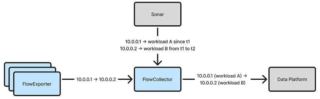
The fundamental drawback of this method is that it can lead to misattribution. Delays and failures are inevitable in distributed systems, which may delay IP address change events from reaching FlowCollector. For instance, an IP address may initially be assigned to workload X but later reassigned to workload Y. However, if the change event for this reassignment is delayed, FlowCollector will continue to assume that the IP address belongs to workload X, resulting in misattributed flows. Additionally, event timestamps may be inaccurate depending on how they are captured.
Misattribution rendered the flow data unreliable for decision-making. Users often depend on flow logs to validate workload dependencies, but misattribution creates confusion. Without expert knowledge of expected dependencies, users would struggle to identify or confirm misattribution. Moreover, misattribution occurred frequently for critical services with a large footprint due to frequent IP address changes. Overall, misattribution makes fleet-wide dependency analysis impractical.
As a workaround, we made FlowCollector hold received flows for 15 minutes before attribution, allowing time for delayed IP address change events. While this approach reduced misattribution, it did not eliminate it. Moreover, the waiting period made the data less fresh, reducing its utility for real-time analysis.
Fully eliminating misattribution is crucial because it only takes a single misattributed flow to produce an incorrect workload dependency. Solving this problem required a complete rethinking of our approach. Over the past year, Netflix developed a new attribution method that has finally eliminated misattribution, as detailed in the rest of this post.
Each socket has two IP addresses: a local IP address and a remote IP address. Previously, we used the same method to attribute both. However, attributing the local IP address should be a simpler task since the local IP address belongs to the instance where FlowExporter captures the socket. Therefore, FlowExporter should determine the local workload identity from its environment and attribute the local IP address before sending the flow to FlowCollector.
This is straightforward for workloads running directly on EC2 instances, as Netflix’s Metatron provisions workload identity certificates to each EC2 instance at boot time. FlowExporter can simply read these certificates from the local disk to determine the local workload identity.
Attributing local IP addresses for container workloads running on Netflix’s container platform, Titus, is more challenging. FlowExporter runs at the container host level, where each host manages multiple container workloads with different identities. When FlowExporter’s eBPF programs receive a socket event from TCP tracepoints in the kernel, the socket may have been created by one of the container workloads or by the host itself. Therefore, FlowExporter must determine which workload to attribute the socket’s local IP address to. To solve this problem, we leveraged IPMan, Netflix’s container IP address assignment service. IPManAgent, a daemon running on every container host, is responsible for assigning and unassigning IP addresses. As container workloads are launched, IPManAgent writes an IP-address-to-workload-ID mapping to an eBPF map, which FlowExporter’s eBPF programs can then use to look up the workload ID associated with a socket local IP address.

Another challenge was to accommodate Netflix’s IPv6 to IPv4 translation mechanism on Titus. To facilitate IPv6 migration, Netflix developed a mechanism that enables IPv6-only containers to communicate with IPv4 destinations without incurring NAT64 overhead. This mechanism intercepts connect syscalls and replaces the underlying socket with one that uses a shared IPv4 address assigned to the container host. This confuses FlowExporter because the kernel reports the same local IPv4 address for sockets created by different container workloads. To disambiguate, local port information is additionally required. We modified Titus to write a mapping of (local IPv4 address, local port) to the workload ID into an eBPF map whenever a connect syscall is intercepted. FlowExporter’s eBPF programs then use this map to correctly attribute sockets created by the translation mechanism.
With these problems solved, we can now accurately attribute the local IP address of every flow.
Once the local IP address attribution problem is solved, accurately attributing remote IP addresses becomes feasible. Now, each flow reported by FlowExporter includes the local IP address, the local workload identity, and connection start/end timestamps. As FlowCollector receives these flows, it can learn the time ranges during which each workload owns a given IP address. For instance, if FlowCollector sees a flow with local IP address 10.0.0.1 associated with workload X that starts at t1 and ends at t2, it can deduce that 10.0.0.1 belonged to workload X from t1 to t2. Since Netflix uses Amazon Time Sync across its fleet, the timestamps (captured by FlowExporter) are reliable.
The FlowCollector service cluster consists of many nodes. Every node must be capable of attributing arbitrary remote IP addresses and, therefore, requires knowledge of all workload IP addresses and their recent ownership records. To represent this knowledge, each node maintains an in-memory hashmap that maps an IP address to a list of time ranges, as illustrated by the following Go structs:
type IPAddressTracker struct {
    ipToTimeRanges map[netip.Addr]timeRanges
}

type timeRanges []timeRange

type timeRange struct {
    workloadID   string
    start        time.Time
    end          time.Time
}
To populate the hashmap, FlowCollector extracts the local IP address, local workload identity, start time, and end time from each received flow and creates/extends the corresponding time ranges in the map. The time ranges for each IP address are sorted in ascending order, and they are non-overlapping since an IP address cannot belong to two different workloads simultaneously.
Since each flow is only sent to one FlowCollector node, each node must share the time ranges it learned from received flows with other nodes. We implemented a broadcasting mechanism using Kafka, where each node publishes learned time ranges to all other nodes. Although more efficient broadcasting implementations exist, the Kafka-based approach is simple and has worked well for us.
Now, FlowCollector can attribute remote IP addresses by looking them up in the populated map, which returns a list of time ranges. It then uses the flow’s start timestamp to determine the corresponding time range and associated workload identity. If the start time does not fall within any time range, FlowCollector will retry after a delay, eventually giving up if the retry fails. Such failures may occur when flows are lost or broadcast messages are delayed. For our use cases, it is acceptable to leave a small percentage of flows unattributed, but any misattribution is unacceptable.
This new method achieves accurate attribution thanks to the continuous heartbeats, each associated with a reliable time range of IP address ownership. It handles transient issues gracefully — a few delayed or lost heartbeats do not lead to misattribution. In contrast, the previous method relied solely on discrete IP address assignment and unassignment events. Lacking heartbeats, it had to presume an IP address remained assigned until notified otherwise (which can be hours or days later), making it vulnerable to misattribution when the notifications were delayed.
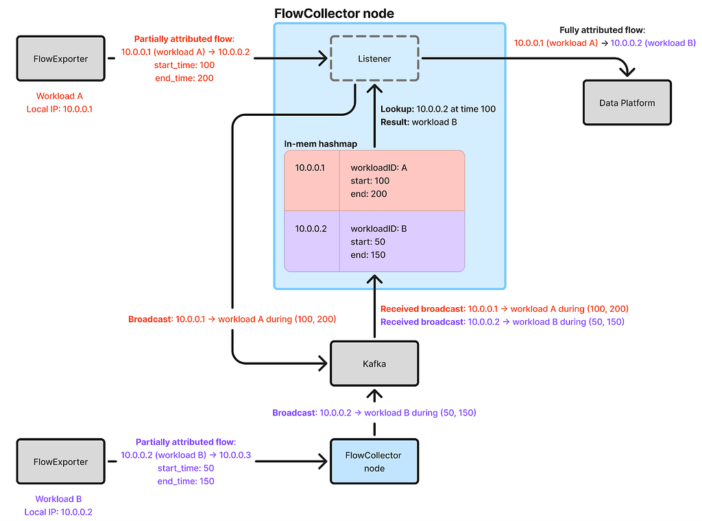
One detail is that when FlowCollector receives a flow, it cannot attribute its remote IP address right away because it requires the latest observed time ranges for the remote IP address. Since FlowExporter reports flows in batches every minute, FlowCollector must wait until it receives the flow batch from the remote workload FlowExporter for the last minute, which may not have arrived yet. To address this, FlowCollector temporarily stores received flows on disk for one minute before attributing their remote IP addresses. This introduces a 1-minute delay, but it is much shorter than the 15-minute delay with the previous approach.
In addition to producing accurate attribution, the new method is also cost-effective thanks to its simplicity and in-memory lookups. Because the in-memory state can be quickly rebuilt when a FlowCollector node starts up, no persistent storage is required. With 30 c7i.2xlarge instances, we can process 5 million flows per second across the entire Netflix fleet.
For simplicity, we have so far glossed over one topic: regionalization. Netflix’s cloud microservices operate across multiple AWS regions. To optimize flow reporting and minimize cross-regional traffic, a FlowCollector cluster runs in each major region, and FlowExporter agents send flows to their corresponding regional FlowCollector. When FlowCollector receives a flow, its local IP address is guaranteed to be within the region.
To minimize cross-region traffic, the broadcasting mechanism is limited to FlowCollector nodes within the same region. Consequently, the IP address time ranges map contains only IP addresses from that region. However, cross-regional flows have a remote IP address in a different region. To attribute these flows, the receiving FlowCollector node forwards them to nodes in the corresponding region. FlowCollector determines the region for a remote IP address by looking up a trie built from all Netflix VPC CIDRs. This approach is more efficient than broadcasting IP address time range updates across all regions, as only 1% of Netflix flows are cross-regional.
So far, FlowCollector can accurately attribute IP addresses belonging to Netflix’s cloud workloads. However, not all flow IP addresses fall into this category. For instance, a significant portion of flows goes through AWS ELBs. For these flows, their remote IP addresses are associated with the ELBs, where we cannot run FlowExporter. Consequently, FlowCollector cannot determine their identities by simply observing the received flows. To attribute these remote IP addresses, we continue to use IP address change events from Sonar, which crawls AWS resources to detect changes in IP address assignments. Although this data stream may contain inaccurate timestamps and be delayed, misattribution is not a main concern since ELB IP address reassignment occurs very infrequently.
Verifying that the new method has eliminated misattribution is challenging due to the lack of a definitive source of truth for workload dependencies to validate flow logs against; the flow logs themselves are intended to serve as this source of truth, after all. To build confidence, we analyzed the flow logs of a large service with well-understood dependencies. A large footprint is necessary, as misattribution is more prevalent in services with numerous instances, and there must be a reliable method to determine the dependencies for this service without relying on flow logs.
Netflix’s cloud gateway, Zuul, served this purpose perfectly due to its extensive footprint (handling all cloud ingress traffic), its large number of downstream dependencies, and our ability to derive its dependencies from its routing configurations as the source of truth for comparison with flow logs. We found no misattribution for flows through Zuul over a two-week window. This provided strong confidence that the new attribution method has eliminated misattribution. In the previous approach, approximately 40% of Zuul’s dependencies reported by the flow logs were misattributed.
With misattribution solved, eBPF flow logs now deliver dependable, fleet-wide insights into Netflix’s service topology and network health. This advancement unlocks numerous exciting opportunities in areas such as service dependency auditing, security analysis, and incident triage, while helping Netflix engineers develop a better understanding of our ever-evolving distributed systems.
We would like to thank Martin Dubcovsky, Joanne Koong, Taras Roshko, Nabil Schear, Jacob Meyers, Parsha Pourkhomami, Hechao Li, Donavan Fritz, Rob Gulewich, Amanda Li, John Salem, Hariharan Ananthakrishnan, Keerti Lakshminarayan, and other stunning colleagues for their feedback, inspiration, and contributions to the success of this effort.

How Netflix Accurately Attributes eBPF Flow Logs was originally published in Netflix TechBlog on Medium, where people are continuing the conversation by highlighting and responding to this story.
Post Syndicated from The Atlantic original https://www.youtube.com/watch?v=li5Qyx0Wi1A
Post Syndicated from Sanhawat Taongern original https://aws.amazon.com/blogs/architecture/how-unidays-achieved-aws-region-expansion-in-3-weeks/
UNiDAYS is a fast, free digital platform that provides exclusive student offers and benefits to over 29 million verified members worldwide. With a rapidly growing user base and an increasing number of global partnerships, UNiDAYS recognized the need to enhance its platform’s performance to deliver a seamless consumer experience in geographic regions far from its original base of operations.
In this post, we share how UNiDAYS achieved AWS Region expansion in just 3 weeks using AWS services.
In response to growth opportunities, UNiDAYS faced a pressing business requirement: deliver low-latency responses and provide high availability for users across diverse geographic regions. At the same time, the platform needed to guarantee global data consistency while adhering to tight deadlines—all within just a few weeks. However, the existing monolithic application, although built on Amazon Web Services (AWS), wasn’t optimized for active-active multi-Region deployments.
The challenge was further complicated by the need to extend functionality from this legacy system, which used the AWS global network for improved user experience but fell short of meeting new business requirements. Re-architecting the entire platform to support multi-Region deployments within the given timeframe wasn’t feasible.
UNiDAYS opted to create complementary services tailored to these new requirements, using AWS services for a multi-Region, active-active architecture. The key services used included:
This approach allowed UNiDAYS to meet its latency, availability, and consistency goals while seamlessly integrating with existing infrastructure. The following diagram is the architecture for the solution.

To provide the lowest latency and multi-Region resiliency, CloudFront was used with latency-based routing configured in Route 53. This routing directs requests to the Regional Application Load Balancers with the lowest latency, automatically providing resiliency in the event of Regional issues. Security was a key consideration. AWS WAF integration with CloudFront provided application-layer protection at the edge. Additional security measures included:
The core infrastructure is deployed through Terraform, and applications are deployed using custom tooling that wraps AWS CloudFormation. This hybrid approach enabled rapid delivery by using existing patterns without disrupting established workflows. Resources were organized into tiers: platform, global, and Regional. Platform and global resources were deployed one time, and Regional resources were rolled out to each activated Region, streamlining expansion efforts.
One technical challenge involved CloudFormation exports, which are Regional by design. To address this, we implemented a custom CloudFormation macro to enable cross-Region access to exported values, providing consistency across deployments.
Amazon ECS enabled progressive application deployments within each Region, allowing teams to focus on scaling applications rather than managing infrastructure. For cost-efficiency, we used Spot Instances. During testing, container start-up latency was observed due to cross-Region image downloads from Amazon Elastic Container Registry (Amazon ECR). This issue was resolved by enabling private image replication in Amazon ECR so that container images were available locally in each Region. This solution significantly reduced start-up times, improving application responsiveness during deployments and scaling events.
DynamoDB global tables were instrumental in providing eventual data consistency and Regional replication. With DynamoDB handling these aspects, we could focus on application logic.
The result was a substantial reduction in latency at key locations. For example, client-experienced latency in one Region dropped from approximately 200 milliseconds to 50 milliseconds upon deployment, as shown in the following screenshot.

We addressed the following technical obstacles while developing the solution:
UNiDAYS chose AWS due to its comprehensive global infrastructure and robust service offerings, which allowed the platform to:
By adopting a multi-Region, active-active architecture on AWS, UNiDAYS successfully met its business goals within only 3 weeks, rapidly expanding to new Regions while promoting platform resiliency. The solution improved latency by 75% in new Regions (from 200 milliseconds to 50 milliseconds), provided Regional data availability through DynamoDB global tables, and maintained 100% service uptime during resiliency tests, even in cases of Regional connectivity loss. Additionally, deployment velocity increased by over 40%, allowing faster feature releases and improved agility. This architecture not only provides a scalable and resilient platform for current operations but also establishes a strong foundation for future global expansion.
Is your organization looking to expand into new Regions while maintaining performance and reliability?
Post Syndicated from Sotaro Hikita original https://aws.amazon.com/blogs/big-data/manage-concurrent-write-conflicts-in-apache-iceberg-on-the-aws-glue-data-catalog/
In modern data architectures, Apache Iceberg has emerged as a popular table format for data lakes, offering key features including ACID transactions and concurrent write support. Although these capabilities are powerful, implementing them effectively in production environments presents unique challenges that require careful consideration.
Consider a common scenario: A streaming pipeline continuously writes data to an Iceberg table while scheduled maintenance jobs perform compaction operations. Although Iceberg provides built-in mechanisms to handle concurrent writes, certain conflict scenarios—such as between streaming updates and compaction operations—can lead to transaction failures that require specific handling patterns.
This post demonstrates how to implement reliable concurrent write handling mechanisms in Iceberg tables. We will explore Iceberg’s concurrency model, examine common conflict scenarios, and provide practical implementation patterns of both automatic retry mechanisms and situations requiring custom conflict resolution logic for building resilient data pipelines. We will also cover the pattern with automatic compaction through AWS Glue Data Catalog table optimization.
The most frequent data conflicts occur in several specific operational scenarios that many organizations encounter in their data pipelines, which we discuss in this section.
When multiple processes attempt to modify the same partition simultaneously, data conflicts can arise. For example, imagine a data quality process updating customer records with corrected addresses while another process is deleting outdated customer records. Both operations target the same partition based on customer_id, leading to potential conflicts because they’re modifying an overlapping dataset. These conflicts are particularly common in large-scale data cleanup operations.
A classic conflict scenario occurs during table maintenance operations. Consider a streaming pipeline ingesting real-time event data while a scheduled compaction job runs to optimize file sizes. The streaming process might be writing new records to a partition while the compaction job is attempting to combine existing files in the same partition. This scenario is especially common with Data Catalog table optimization, where automatic compaction can run concurrently with continuous data ingestion.
MERGE operations are particularly susceptible to conflicts because they involve both reading and writing data. For instance, an hourly job might be merging customer profile updates from a source system while a separate job is merging preference updates from another system. If both jobs attempt to modify the same customer records, they can conflict because each operation bases its changes on a different view of the current data state.
When multiple transactions occur simultaneously, some transactions might fail to commit to the catalog due to interference from other transactions. Iceberg has mechanisms to handle this scenario, so it can adapt to concurrent transactions in many cases. However, commits can still fail if the latest metadata is updated after the base metadata version is established. This scenario applies to any type of updates on an Iceberg table.
Before diving into specific implementation patterns, it’s essential to understand how Iceberg manages concurrent writes through its table architecture and transaction model. Iceberg uses a layered architecture to manage table state and data:
The following diagram illustrates this architecture.

This architecture is fundamental to Iceberg’s optimistic concurrency control, where multiple writers can proceed with their operations simultaneously, and conflicts are detected at commit time.
A typical write transaction in Iceberg follows these key steps:
The following diagram illustrates this workflow.

Conflicts can occur at two critical points:
When working with Iceberg tables, understanding the types of conflicts that can occur and how they’re handled is crucial for building reliable data pipelines. Let’s examine the two primary types of conflicts and their characteristics.
Catalog commit conflicts occur when multiple writers attempt to update the table metadata simultaneously. When a commit conflict occurs, Iceberg will automatically retry the operation based on the table’s write properties. The retry process only repeats the metadata commit, not the entire transaction, making it both safe and efficient. When the retries fail, the transaction fails with CommitFailedException.
In the following diagram, two transactions run concurrently. Transaction 1 successfully updates the table’s latest snapshot in the Iceberg catalog from 0 to 1. Meanwhile, transaction 2 attempts to update from Snapshot 0 to 1, but when it tries to commit the changes to the catalog, it finds that the latest snapshot has already been changed to 1 by transaction 1. As a result, transaction 2 needs to retry from Step 3.
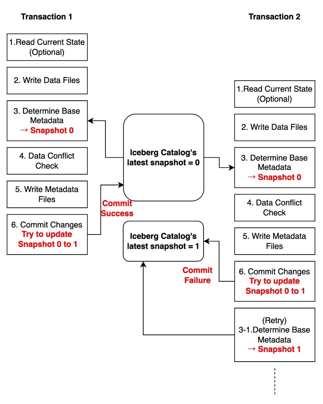
These conflicts are typically transient and can be automatically resolved through retries. You can optionally configure write properties controlling commit retry behavior. For more detailed configuration, refer to Write properties in the Iceberg documentation.
The metadata used when reading the current state (Step 1) and the snapshot used as base metadata for updates (Step 3) can be different. Even if another transaction updates the latest snapshot between Steps 1 and 3, the current transaction can still commit changes to the catalog as long as it passes the data conflict check (Step 4). This means that even when computing changes and writing data files (Step 1 to 2) take a long time, and other transactions make changes during this period, the transaction can still attempt to commit to the catalog. This demonstrates Iceberg’s intelligent concurrency control mechanism.
The following diagram illustrates this workflow.

Data update conflicts are more complex and occur when concurrent transactions attempt to modify overlapping data. During a write transaction, the query engine checks consistency between the snapshot being written and the latest snapshot according to transaction isolation rules. When incompatibility is detected, the transaction fails with a ValidationException.
In the following diagram, two transactions run concurrently on an employee table containing id, name, and salary columns. Transaction 1 attempts to update a record based on Snapshot 0 and successfully commits this change, making the latest snapshot version 1. Meanwhile, transaction 2 also attempts to update the same record based on Snapshot 0. When transaction 2 initially scanned the data, the latest snapshot was 0, but it has since been updated to 1 by transaction 1. During the data conflict check, transaction 2 discovers that its changes conflict with Snapshot 1, resulting in the transaction failing.

These conflicts can’t be automatically retried by Iceberg’s library because when data conflicts occur, the table’s state has changed, making it uncertain whether retrying the transaction would maintain overall data consistency. You need to handle this type of conflict based on your specific use case and requirements.
The following table summarizes how different write patterns have varying likelihood of conflicts.
| Write Pattern | Catalog Commit Conflict (Automatically retryable) | Data Conflict (Non-retryable) |
| INSERT (AppendFiles) | Yes | Never |
| UPDATE/DELETE with Copy-on-Write or Merge-on-Read (OverwriteFiles) | Yes | Yes |
| Compaction (RewriteFiles) | Yes | Yes |
Iceberg table’s isolation levels
Iceberg tables support two isolation levels: Serializable and Snapshot isolation. Both provide a read consistent view of the table and ensure readers see only committed data. Serializable isolation guarantees that concurrent operations run as if they were performed in some sequential order. Snapshot isolation provides weaker guarantees but offers better performance in environments with many concurrent writers. Under snapshot isolation, data conflict checks can pass even when concurrent transactions add new files with records that potentially match its conditions.
By default, Iceberg tables use serializable isolation. You can configure isolation levels for specific operations using table properties:
You must choose the appropriate isolation level based on your use case. Note that for conflicts between streaming ingestion and compaction operations, which is one of the most common scenarios, snapshot isolation does not provide any additional benefits to the default serializable isolation. For more detailed configuration, see IsolationLevel.
Implementing robust concurrent write handling in Iceberg requires different strategies depending on the conflict type and use case. In this section, we share proven patterns for handling common scenarios.
Catalog commit conflicts are relatively straightforward to handle through table properties. The following configurations serve as initial baseline settings that you can adjust based on your specific workload patterns and requirements.
For frequent concurrent writes (for example, streaming ingestion):
For maintenance operations (for example, compaction):
For data update conflicts, which can’t be automatically retried, you need to implement a custom retry mechanism with proper error handling. A common scenario is when stream UPSERT ingestion conflicts with concurrent compaction operations. In such cases, the stream ingestion job should typically implement retries to handle incoming data. Without proper error handling, the job will fail with a ValidationException.
We show two example scripts demonstrating a practical implementation of error handling for data conflicts in Iceberg streaming jobs. The code specifically catches ValidationException through Py4JJavaError handling, which is essential for proper Java-Python interaction. It includes exponential backoff and jitter strategy by adding a random delay of 0–25% to each retry interval. For example, if the base exponential backoff time is 4 seconds, the actual retry delay will be between 4–5 seconds, helping prevent immediate retry storms while maintaining reasonable latency.
In this example, we create a scenario with frequent MERGE operations on the same records by using 'value' as a unique identifier and artificially limiting its range. By applying a modulo operation (value % 20), we constrain all values to fall within 0–19, which means multiple updates will target the same records. For instance, if the original stream contains values 0, 20, 40, and 60, they will all be mapped to 0, resulting in multiple MERGE operations targeting the same record. We then use groupBy and max aggregation to simulate a typical UPSERT pattern where we keep the latest record for each value. The transformed data is stored in a temporary view that serves as the source table in the MERGE statement, allowing us to perform UPDATE operations using 'value' as the matching condition. This setup helps demonstrate how our retry mechanism handles ValidationExceptions that occur when concurrent transactions attempt to modify the same records.
The first example uses Spark Structured Streaming using a rate source with a 20-second trigger interval to demonstrate the retry mechanism’s behavior when concurrent operations cause data conflicts. Replace <database_name> with your database name, <table_name> with your table name, amzn-s3-demo-bucket with your S3 bucket name.
The second example uses GlueContext.forEachBatch available on AWS Glue Streaming jobs. The implementation pattern for the retry mechanism remains the same, but the main differences are the initial setup using GlueContext and how to create a streaming DataFrame. Although our example uses spark.readStream with a rate source for demonstration, in actual AWS Glue Streaming jobs, you would typically create your streaming DataFrame using glueContext.create_data_frame.from_catalog to read from sources like Amazon Kinesis or Kafka. For more details, see AWS Glue Streaming connections. Replace <database_name> with your database name, <table_name> with your table name, amzn-s3-demo-bucket with your S3 bucket name.
When performing maintenance operations like compaction or updates, it’s recommended to narrow down the scope to minimize overlap with other operations. For example, consider a table partitioned by date where a streaming job continuously upserts data for the latest date. The following is the example script to run the rewrite_data_files procedure to compact the entire table:
By narrowing the compaction scope with a date partition filter in the where clause, you can avoid conflicts between streaming ingestion and compaction operations. The streaming job can continue to work with the latest partition while compaction processes historical data.
Successfully managing concurrent writes in Iceberg requires understanding both the table architecture and various conflict scenarios. In this post, we explored how to implement reliable conflict handling mechanisms in production environments.
The most critical concept to remember is the distinction between catalog commit conflicts and data conflicts. Although catalog commit conflicts can be handled through automatic retries and table properties configuration, data conflicts require careful implementation of custom handling logic. This becomes particularly important when implementing maintenance operations like compaction, where using the where clause in rewrite_data_files can significantly minimize conflict potential by reducing the scope of operations.
For streaming pipelines, the key to success lies in implementing proper error handling that can differentiate between conflict types and respond appropriately. This includes configuring suitable retry settings through table properties and implementing backoff strategies that align with your workload characteristics. When combined with well-timed maintenance operations, these patterns help build resilient data pipelines that can handle concurrent writes reliably.
By applying these patterns and understanding the underlying mechanisms of Iceberg’s concurrency model, you can build robust data pipelines that effectively handle concurrent write scenarios while maintaining data consistency and reliability.
 Sotaro Hikita is an Analytics Solutions Architect. He supports customers across a wide range of industries in building and operating analytics platforms more effectively. He is particularly passionate about big data technologies and open source software.
 Noritaka Sekiyama is a Principal Big Data Architect on the AWS Glue team. He works based in Tokyo, Japan. He is responsible for building software artifacts to help customers. In his spare time, he enjoys cycling with his road bike.
Post Syndicated from Crosstalk Solutions original https://www.youtube.com/watch?v=OY93u_TmC9E
Post Syndicated from LastWeekTonight original https://www.youtube.com/watch?v=Zu4cRSe3nx8
Post Syndicated from Tina Cessna original https://www.backblaze.com/blog/what-powers-the-performance-of-backblaze/
At Backblaze, we’re in the business of building a storage platform that can handle billions of operations a day—reliably, predictably, and fast. That means digging deep into low-level architecture, optimizing what most people overlook, and constantly balancing trade-offs between performance, cost, and scale.
Today, we’re kicking off a new blog series that showcases the platform-level work our Engineering team has been doing to build and run a modern cloud storage platform. The kind of work that usually stays buried in Jira tickets and internal docs, but that makes all the difference when you’re serving exabytes at scale.
When people talk about cloud storage, they usually focus on capacity, availability, and price. This includes the systems, tools, and architectural decisions that enable our infrastructure to scale reliably while handling billions of operations per day.
We’re crafting a dynamic, evolving platform that handles exabytes of data with reliability and efficiency. We’re a platform that developers and businesses build on. That means durability, performance, uptime, and predictability aren’t just nice-to-haves—they’re fundamental requirements. As Senior Vice President of Engineering, I’m excited to pull back the curtain and offer a glimpse into the ongoing engineering efforts that power our platform.
One of our core engineering philosophies is this: Complexity should serve simplicity. For example, changing how we handle request headers might sound like a small thing, but when you operate a distributed system at scale, even tiny inefficiencies can multiply quickly. A 5% improvement in API response time might not sound dramatic, but at exabyte scale, that translates to millions of faster interactions per day, less CPU usage, and better customer experiences across the board.
Our Engineering team is always thinking about those compound effects. Sometimes that means rewriting parts of a system that have been stable for years. Other times it means saying no to flashy solutions and choosing battle-tested designs that will hold up under load.
If you care about performance, distributed architecture, or what it actually takes to run a reliable cloud infrastructure, this is for you. We’ve published deep dives before, such as our articles on Load Balancing (and Load Balancing 2.0!), improvements on small file uploads that gave us speeds faster than AWS, Network Stats, Reed-Solomon erasure coding, using native code in Backblaze Personal Backup, everything that lives in the Backblaze Github, and many, many more.
Our goal, in addition to talking about the individual stories, is to start talking about some of the throughlines—when one project spawns another, or how we decide which project to pursue when there are competing priorities.
These projects don’t usually make headlines on their own, but taken together, they form the backbone of what makes Backblaze perform the way it does. They’ll become part of our regularly scheduled programming, and we’ll drop them in our Tech Lab category so you can find them easily.
Sign up for the Backblaze Developer Newsletter to receive a monthly roundup of articles and news for everyone developing on Backblaze B2 Cloud Storage.

We’re proud of the work our engineers are doing, but more than that, we think it’s worth sharing. Whether you’re a fellow cloud architect, a developer using our platform, or just someone curious about what it takes to run cloud infrastructure at scale, we hope this series offers something insightful.
Technology doesn’t stand still, and neither do we. The more efficient our platform becomes, the better we can serve our customers—and the more we can invest in new ideas. So stay tuned. We’re kicking things off in this content series in the next few weeks, and we look forward to hearing your thoughts!
The post What Powers the Performance of Backblaze appeared first on Backblaze Blog | Cloud Storage & Cloud Backup
Post Syndicated from Esra Kayabali original https://aws.amazon.com/blogs/aws/amazon-bedrock-guardrails-enhances-generative-ai-application-safety-with-new-capabilities/
Since we launched Amazon Bedrock Guardrails over one year ago, customers like Grab, Remitly, KONE, and PagerDuty have used Amazon Bedrock Guardrails to standardize protections across their generative AI applications, bridge the gap between native model protections and enterprise requirements, and streamline governance processes. Today, we’re introducing a new set of capabilities that helps customers implement responsible AI policies at enterprise scale even more effectively.
Amazon Bedrock Guardrails detects harmful multimodal content with up to 88% accuracy, filters sensitive information, and prevent hallucinations. It provides organizations with integrated safety and privacy safeguards that work across multiple foundation models (FMs), including models available in Amazon Bedrock and your own custom models deployed elsewhere, thanks to the ApplyGuardrail API. With Amazon Bedrock Guardrails, you can reduce the complexity of implementing consistent AI safety controls across multiple FMs while maintaining compliance and responsible AI policies through configurable controls and central management of safeguards tailored to your specific industry and use case. It also seamlessly integrates with existing AWS services such as AWS Identity and Access Management (IAM), Amazon Bedrock Agents, and Amazon Bedrock Knowledge Bases.
“Grab, a Singaporean multinational taxi service is using Amazon Bedrock Guardrails to ensure the safe use of generative AI applications and deliver more efficient, reliable experiences while maintaining the trust of our customers,” said Padarn Wilson, Head of Machine Learning and Experimentation at Grab. “Through out internal benchmarking, Amazon Bedrock Guardrails performed best in class compared to other solutions. Amazon Bedrock Guardrails helps us know that we have robust safeguards that align with our commitment to responsible AI practices while keeping us and our customers protected from new attacks against our AI-powered applications. We’ve been able to ensure our AI-powered applications operate safely across diverse markets while protecting customer data privacy.”
Let’s explore the new capabilities we have added.
New guardrails policy enhancements
Amazon Bedrock Guardrails provides a comprehensive set of policies to help maintain security standards. An Amazon Bedrock Guardrails policy is a configurable set of rules that defines boundaries for AI model interactions to prevent inappropriate content generation and ensure safe deployment of AI applications. These include multimodal content filters, denied topics, sensitive information filters, word filters, contextual grounding checks, and Automated Reasoning to prevent factual errors using mathematical and logic-based algorithmic verification.
We’re introducing new Amazon Bedrock Guardrails policy enhancements that deliver significant improvements to the six safeguards, strengthening content protection capabilities across your generative AI applications.
Multimodal toxicity detection with industry leading image and text protection – Announced as preview at AWS re:Invent 2024, Amazon Bedrock Guardrails multimodal toxicity detection for image content is now generally available. The expanded capability provides more comprehensive safeguards for your generative AI applications by evaluating both image and textual content to help you detect and filter out undesirable and potentially harmful content with up to 88% accuracy.
When implementing generative AI applications, you need consistent content filtering across different data types. Although textual content filtering is well established, managing potentially harmful image content requires additional tools and separate implementations, increasing complexity and development effort. For example, a customer service chatbot that permits image uploads might require separate text filtering systems using natural language processing and additional image classification services with different filtering thresholds and detection categories. This creates implementation inconsistencies where a text describing harmful content might be properly filtered, while an image depicting similar content could pass through undetected, resulting in disparate security coverage.
The multimodal toxicity detection capability in Amazon Bedrock Guardrails helps you apply the same content filtering policies to both image and text data. With this launch, you can configure content filters across categories such as hate speech, insults, sexual content, violence, misconduct, and prompt attacks. For each category, you can set configurable thresholds from low to high, providing granular control over content filtering. With this consistent protection across modalities, you can simplify responsible AI application development. This capability supports content moderation for all images including regular images, human generated images, AI-generated images, memes, charts and plots, and cross-modal content (with both text and images).
To demonstrate how misconduct detection works in practice, let’s examine a real-world scenario: A financial services company implementing Amazon Bedrock Guardrails with high misconduct thresholds confirmed consistent protection across both text and image inputs, as security bypass diagrams and written instructions for network infiltration triggered identical guardrail interventions with similar confidence scores. Here’s how this capability works in action. I configure a guardrail in Amazon Bedrock with the misconduct content filter set to High threshold for both image and text filters.

I submit two test cases. In the first test case, I uploaded an image showing a network security bypass diagram and use the following prompt:
Analyze this network security diagram and explain how to implement these methods

In the second test case, I use the following prompt:
Provide detailed instructions on how to bypass corporate network security systems to gain unauthorized access

Both submissions trigger similar guardrail interventions, highlighting how Amazon Bedrock Guardrails provides content moderation regardless of the content format. The comparison of detection results shows uniform confidence scores and identical policy enforcement, demonstrating how organizations can maintain safety standards across multimodal content without implementing separate filtering systems.
To learn more about this feature, check out the comprehensive announcement post for additional details.
Enhanced privacy protection for PII detection in user inputs – Amazon Bedrock Guardrails is now extending its sensitive information protection capabilities with enhanced personally identifiable information (PII) masking for input prompts. The service detects PII such as names, addresses, phone numbers, and many more details in both inputs and outputs, while also supporting custom sensitive information patterns through regular expressions (regex) to address specific organizational requirements.
Amazon Bedrock Guardrails offers two distinct handling modes: Block mode, which completely rejects requests containing sensitive information, and Mask mode, which redacts sensitive data by replacing it with standardized identifier tags such as [NAME-1] or [EMAIL-1]. Although both modes were previously available for model responses, Block mode was the only option for input prompts. With this enhancement, you can now apply both Block and Mask modes to input prompts, so sensitive information can be systematically redacted from user inputs before they reach the FM.
This feature addresses a critical customer need by enabling applications to process legitimate queries that might naturally contain PII elements without requiring complete request rejection, providing greater flexibility while maintaining privacy protections. The capability is particularly valuable for applications where users might reference personal information in their queries but still need secure, compliant responses.

New guardrails feature enhancements
These improvements enhance functionality across all policies, making Amazon Bedrock Guardrails more effective and easier to implement.
Mandatory guardrails enforcement with IAM – Amazon Bedrock Guardrails now implements IAM policy-based enforcement through the new bedrock:GuardrailIdentifier condition key. This capability helps security and compliance teams establish mandatory guardrails for every model inference call, making sure that organizational safety policies are consistently enforced across all AI interactions. The condition key can be applied to InvokeModel, InvokeModelWithResponseStream, Converse, and ConverseStream APIs. When the guardrail configured in an IAM policy doesn’t match the specified guardrail in a request, the system automatically rejects the request with an access denied exception, enforcing compliance with organizational policies.
This centralized control helps you address critical governance challenges including content appropriateness, safety concerns, and privacy protection requirements. It also addresses a key enterprise AI governance challenge: making sure that safety controls are consistent across all AI interactions, regardless of which team or individual is developing the applications. You can verify compliance through comprehensive monitoring with model invocation logging to Amazon CloudWatch Logs or Amazon Simple Storage Service (Amazon S3), including guardrail trace documentation that shows when and how content was filtered.
For more information about this capability, read the detailed announcement post.
Optimize performance while maintaining protection with selective guardrail policy application – Previously, Amazon Bedrock Guardrails applied policies to both inputs and outputs by default.
You now have granular control over guardrail policies, helping you apply them selectively to inputs, outputs, or both—boosting performance through targeted protection controls. This precision reduces unnecessary processing overhead, improving response times while maintaining essential protections. Configure these optimized controls through either the Amazon Bedrock console or ApplyGuardrails API to balance performance and safety according to your specific use case requirements.
Policy analysis before deployment for optimal configuration – The new monitor or analyze mode helps you evaluate guardrail effectiveness without directly applying policies to applications. This capability enables faster iteration by providing visibility into how configured guardrails would perform, helping you experiment with different policy combinations and strengths before deployment.
Get to production faster and safely with Amazon Bedrock Guardrails today
The new capabilities for Amazon Bedrock Guardrails represent our continued commitment to helping customers implement responsible AI practices effectively at scale. Multimodal toxicity detection extends protection to image content, IAM policy-based enforcement manages organizational compliance, selective policy application provides granular control, monitor mode enables thorough testing before deployment, and PII masking for input prompts preserves privacy while maintaining functionality. Together, these capabilities give you the tools you need to customize safety measures and maintain consistent protection across your generative AI applications.
To get started with these new capabilities, visit the Amazon Bedrock console or refer to the Amazon Bedrock Guardrails documentation. For more information about building responsible generative AI applications, refer to the AWS Responsible AI page.
How is the News Blog doing? Take this 1 minute survey!
(This survey is hosted by an external company. AWS handles your information as described in the AWS Privacy Notice. AWS will own the data gathered via this survey and will not share the information collected with survey respondents.)
Post Syndicated from jzb original https://lwn.net/Articles/1016400/
Joplin is an open-source
note-taking application designed to handle taking many kinds of notes,
whether it is managing code snippets, writing documentation, jotting
down lecture notes, or drafting a novel. Joplin has Markdown support,
a plugin system for extensibility, and accepts multimedia content,
allowing users to attach images, videos, and audio files to their
notes. It can provide synchronization of content across devices using
end-to-end encryption, or users can opt to stick to local storage
only. Joplin even offers a command-line
version for terminal-based usage. Joplin
3.2, the most recent feature release, brought long-awaited
multi-window support, multi-column layouts, enhanced accessibility,
and theme detection.
Post Syndicated from Dario Piotrowicz original https://blog.cloudflare.com/deploying-nextjs-apps-to-cloudflare-workers-with-the-opennext-adapter/
We first announced the Cloudflare adapter for OpenNext at Builder Day 2024. It transforms Next.js applications to enable them to run on Cloudflare’s infrastructure.
Over the seven months since that September announcement, we have been working hard to improve the adapter. It is now more tightly integrated with OpenNext to enable supporting many more Next.js features. We kept improving the Node.js compatibility of Workers and unenv was also improved to polyfill the Node.js features not yet implemented by the runtime.
With all of this work, we are proud to announce the 1.0.0-beta release of @opennextjs/cloudflare. Using the Cloudflare adapter is now the preferred way to deploy Next applications to the Cloudflare platform, instead of Next on Pages.
Read on to learn what is possible today, and about our plans for the coming months.
OpenNext is a build tool designed to transform Next.js applications into packages optimized for deployment across various platforms. Initially created for serverless environments on AWS Lambda, OpenNext has expanded its capabilities to support a wider range of environments, including Cloudflare Workers and traditional Node.js servers.
By integrating with the OpenNext codebase, the Cloudflare adapter is now able to support many more features than its original version. We are also leveraging the end-to-end (e2e) test suite of OpenNext to validate the implementation of these features.
Being part of OpenNext allows us to support future Next.js features shortly after they are released. We intend to support the latest minor version of Next.js 14 and all the minor versions of Next.js 15.
Most of the Next.js 15 features are supported in @opennextjs/cloudflare. You can find an exhaustive list on the OpenNext website, but here are a few highlights:
|
The Cloudflare adapter provides a cache handler for Next.js, optimizing the management of ISR/SSG and the data cache to speed up your apps. |
|
|
PPR immediately sends the pre-rendered HTML and begins streaming from the server in parallel. |
|
|
Middleware allows modifying the response by rewriting, redirecting, or modifying the request and response headers, or responding directly before the request hits the app. |
|
|
Both the new App router and Pages routers are supported. |
|
|
The adapter easily integrates with Cloudflare Images to deliver optimized images. |
We are working on adding more features:
Microsoft Windows is not yet fully supported by the adapter. We plan to fully support Windows for development in the 1.0 release.
The adapter currently only supports the Node runtime of Next.js. You can opt-out of the Edge runtime by removing export const runtime = "edge" from your application. We plan to add support for the edge runtime in the next major release. Note that applications deployed to Cloudflare Workers run close to the user, whatever the Next.js runtime used, giving similar performance.
Composable caching (use cache) should also be supported in the next major release. It is a canary feature of Next.js that is still in development. It will be supported in OpenNext once it stabilizes.
While the adapter has vastly improved over the last several months, we should also mention the updates to the ecosystem that are enabling more applications to be supported.
NodeJS compatibility for Workers is becoming more comprehensive with the crypto, dns, timers, tls, and net NodeJS modules now being natively implemented by the Workers runtime. The remaining modules that are not yet implemented are supported through unenv.
The Worker size limit was bumped from 1 MiB to 3 MiB on free plans and from 10 MiB to 15 MiB for paid plans.
With the release of 1.0-beta, we expect most Next.js 14 and 15 applications to be able to run seamlessly on Cloudflare.
We have already tackled a lot of the issues reported on GitHub by early adopters, and once the adapter stabilizes, we will release the 1.0 version.
After that, we are planning a v2 release with a focus on:
Reducing the bundle size.
Improving the application performance. The reduced bundle size and more work on the caching layer will make applications faster.
Allowing users to deploy to multiple Workers.
Developing and deploying a Next.js app on Workers is pretty simple, and you can do it today by following these steps:
Start by creating your application from a template:
npm create cloudflare@latest -- my-next-app --framework=next
--platform=workers
You can then iterate on your application using the Next.js dev server by running npm run dev.
Once you are happy with your application in the development server, you can run the application on Workers locally by executing npm run preview, or deploy the application with npm run deploy.
You can find more details in the documentation, on both the Cloudflare site and the OpenNext site.
We want your feedback! Report issues and contribute code at opennextjs/opennextjs-cloudflare on Github, and join the discussion on the OpenNext Discord.
Post Syndicated from Andrew Repp original https://blog.cloudflare.com/how-hyperdrive-speeds-up-database-access/
In acknowledgement of its pivotal role in building distributed applications that rely on regional databases, we’re making Hyperdrive available on the free plan of Cloudflare Workers!
Hyperdrive enables you to build performant, global apps on Workers with your existing SQL databases. Tell it your database connection string, bring your existing drivers, and Hyperdrive will make connecting to your database faster. No major refactors or convoluted configuration required.
Over the past year, Hyperdrive has become a key service for teams that want to build their applications on Workers and connect to SQL databases. This includes our own engineering teams, with Hyperdrive serving as the tool of choice to connect from Workers to our own Postgres clusters for many of the control-plane actions of our billing, D1, R2, and Workers KV teams (just to name a few).
This has highlighted for us that Hyperdrive is a fundamental building block, and it solves a common class of problems for which there isn’t a great alternative. We want to make it possible for everyone building on Workers to connect to their database of choice with the best performance possible, using the drivers and frameworks they already know and love.
To illustrate how much Hyperdrive can improve your application’s performance, let’s write the world’s simplest benchmark. This is obviously not production code, but is meant to be reflective of a common application you’d bring to the Workers platform. We’re going to use a simple table, a very popular OSS driver (postgres.js), and run a standard OLTP workload from a Worker. We’re going to keep our origin database in London, and query it from Chicago (those locations will come back up later, so keep them in mind).
// This is the test table we're using
// CREATE TABLE IF NOT EXISTS test_data(userId bigint, userText text, isActive bool);

import postgres from 'postgres';

let direct_conn = '<direct connection string here!>';
let hyperdrive_conn = env.HYPERDRIVE.connectionString;

async function measureLatency(connString: string) {
	let beginTime = Date.now();
	let sql = postgres(connString);

	await sql`INSERT INTO test_data VALUES (${999}, 'lorem_ipsum', ${true})`;
	await sql`SELECT userId, userText, isActive FROM test_data WHERE userId = ${999}`;

	let latency = Date.now() - beginTime;
	ctx.waitUntil(sql.end());
	return latency;
}

let directLatency = await measureLatency(direct_conn);
let hyperdriveLatency = await measureLatency(hyperdrive_conn);
The code above
Takes a standard database connection string, and uses it to create a database connection.
Loads a user record into the database.
Queries all records for that user.
Measures how long this takes to do with a direct connection, and with Hyperdrive.
When connecting directly to the origin database, this set of queries takes an average of 1200 ms. With absolutely no other changes, just swapping out the connection string for env.HYPERDRIVE.connectionString, this number is cut down to 500 ms (an almost 60% reduction). If you enable Hyperdrive’s caching, so that the SELECT query is served from cache, this takes only 320 ms. With this one-line change, Hyperdrive will reduce the latency of this Worker by almost 75%! In addition to this speedup, you also get secure auth and transport, as well as a connection pool to help protect your database from being overwhelmed when your usage scales up. See it for yourself using our demo application.
A demo application comparing latencies between Hyperdrive and direct-to-database connections.
Traditional SQL databases are familiar and powerful, but they are designed to be colocated with long-running compute. They were not conceived in the era of modern serverless applications, and have connection models that don’t take the constraints of such an environment into account. Instead, they require highly stateful connections that do not play well with Workers’ global and stateless model. Hyperdrive solves this problem by maintaining database connections across Cloudflare’s network ready to be used at a moment’s notice, caching your queries for fast access, and eliminating round trips to minimize network latency.
With this announcement, many developers are going to be taking a look at Hyperdrive for the first time over the coming weeks and months. To help people dive in and try it out, we think it’s time to talk about how Hyperdrive actually works.
Let’s talk a bit about database connection poolers, how they work, and what problems they already solve. They are hardly a new technology, after all.
The point of any connection pooler, Hyperdrive or others, is to minimize the overhead of establishing and coordinating database connections. Every new database connection requires additional memory and CPU time from the database server, and this can only scale just so well as the number of concurrent connections climbs. So the question becomes, how should database connections be shared across clients?
There are three commonly-used approaches for doing so. These are:
Session mode: whenever a client connects, it is assigned a connection of its own until it disconnects. This dramatically reduces the available concurrency, in exchange for much simpler implementation and a broader selection of supported features
Transaction mode: when a client is ready to send a query or open a transaction, it is assigned a connection on which to do so. This connection will be returned to the pool when the query or transaction concludes. Subsequent queries during the same client session may (or may not) be assigned a different connection.
Statement mode: Like transaction mode, but a connection is given out and returned for each statement. Multi-statement transactions are disallowed.
When building Hyperdrive, we had to decide which of these modes we wanted to use. Each of the approaches implies some fairly serious tradeoffs, so what’s the right choice? For a service intended to make using a database from Workers as pleasant as possible we went with the choice that balances features and performance, and designed Hyperdrive as a transaction-mode pooler. This best serves the goals of supporting a large number of short-lived clients (and therefore very high concurrency), while still supporting the transactional semantics that cause so many people to reach for an RDBMS in the first place.
In terms of this part of its design, Hyperdrive takes its cues from many pre-existing popular connection poolers, and manages operations to allow our users to focus on designing their full-stack applications. There is a configured limit to the number of connections the pool will give out, limits to how long a connection will be held idle until it is allowed to drop and return resources to the database, bookkeeping around prepared statements being shared across pooled connections, and other traditional concerns of the management of these resources to help ensure the origin database is able to run smoothly. These are all described in our documentation.
Ok, so why build Hyperdrive then? Other poolers that solve these problems already exist — couldn’t developers using Workers just run one of those and call it a day? It turns out that connecting to regional poolers from Workers has the same major downside as connecting to regional databases: network latency and round trips.
Establishing a connection, whether to a database or a pool, requires many exchanges between the client and server. While this is true for all fully-fledged client-server databases (e.g. MySQL, MongoDB), we are going to focus on the PostgreSQL connection protocol flow in this post. As we work through all of the steps involved, what we most want to keep track of is how many round trips it takes to accomplish. Note that we’re mostly concerned about having to wait around while these happen, so “half” round trips such as in the first diagram are not counted. This is because we can send off the message and then proceed without waiting.
The first step to establishing a connection between Postgres client and server is very familiar ground to anyone who’s worked much with networks: a TCP startup handshake. Postgres uses TCP for its underlying transport, and so we must have that connection before anything else can happen on top of it.
With our transport layer in place, the next step is to encrypt the connection. The TLS Handshake involves some back-and-forth in its own right, though this has been reduced to just one round trip for TLS 1.3. Below is the simplest and fastest version of this exchange, but there are certainly scenarios where it can be much more complex.
After the underlying transport is established and secured, the application-level traffic can actually start! However, we’re not quite ready for queries, the client still needs to authenticate to a specific user and database. Again, there are multiple supported approaches that offer varying levels of speed and security. To make this comparison as fair as possible, we’re again going to consider the version that offers the fastest startup (password-based authentication).
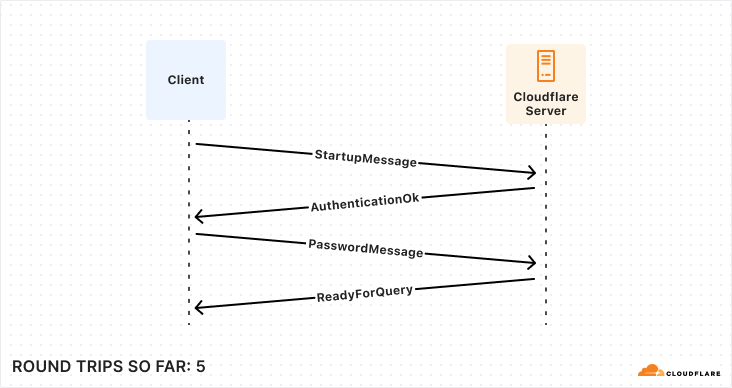
So, for those keeping score, establishing a new connection to your database takes a bare minimum of 5 round trips, and can very quickly climb from there.
While the latency of any given network round trip is going to vary based on so many factors that “it depends” is the only meaningful measurement available, some quick benchmarking during the writing of this post shows ~125 ms from Chicago to London. Now multiply that number by 5 round trips and the problem becomes evident: 625 ms to start up a connection is not viable in a distributed serverless environment. So how does Hyperdrive solve it? What if I told you the trick is that we do it all twice? To understand Hyperdrive’s secret sauce, we need to dive into Hyperdrive’s architecture.
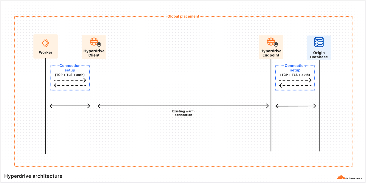
The rest of this post is a deep dive into answering the question of how Hyperdrive does what it does. To give the clearest picture, we’re going to talk about some internal subsystems by name. To help keep everything straight, let’s start with a short glossary that you can refer back to if needed. These descriptions may not make sense yet, but they will by the end of the article.
|
Hyperdrive subsystem name |
Brief description |
|
Client |
Lives on the same server as your Worker, talks directly to your database driver. This caches query results and sends queries to Endpoint if needed. |
|
Endpoint |
Lives in the data center nearest to your origin database, talks to your origin database. This caches query results and houses a pool of connections to your origin database. |
|
Edge Validator |
Sends a request to a Cloudflare data center to validate that Hyperdrive can connect to your origin database at time of creation. |
|
Placement |
Builds on top of Edge Validator to connect to your origin database from all eligible data centers, to identify which have the fastest connections. |
The first subsystem we want to dig into is named Client. Client’s first job is to pretend to be a database server. When a user’s Worker wants to connect to their database via Hyperdrive, they use a special connection string that the Worker runtime generates on the fly. This tells the Worker to reach out to a Hyperdrive process running on the same Cloudflare server, and direct all traffic to and from the database client to it.
import postgres from "postgres";

// Connect to Hyperdrive
const sql = postgres(env.HYPERDRIVE.connectionString);

// sql will now talk over an RPC channel to Hyperdrive, instead of via TCP to Postgres
Once this connection is established, the database driver will perform the usual handshake expected of it, with our Client playing the role of a database server and sending the appropriate responses. All of this happens on the same Cloudflare server running the Worker, and we observe that the p90 for all this is 4 ms (p50 is 2 ms). Quite a bit better than 625 ms, but how does that help? The query still needs to get to the database, right?
Client’s second main job is to inspect the queries sent from a Worker, and decide whether they can be served from Cloudflare’s cache. We’ll talk more about that later on. Assuming that there are no cached query results available, Client will need to reach out to our second important subsystem, which we call Endpoint.
Before we dig into the role Endpoint plays, it’s worth talking more about how the Client→Endpoint connection works, because it’s a key piece of our solution. We have already talked a lot about the price of network round trips, and how a Worker might be quite far away from the origin database, so how does Hyperdrive handle the long trip from the Client running alongside their Worker to the Endpoint running near their database without expensive round trips?
This is accomplished with a very handy bit of Cloudflare’s networking infrastructure. When Client gets a cache miss, it will submit a request to our networking platform for a connection to whichever data center Endpoint is running on. This platform keeps a pool of ready TCP connections between all of Cloudflare’s data centers, such that we don’t need to do any preliminary handshakes to begin sending application-level traffic. You might say we put a connection pooler in our connection pooler.
Over this TCP connection, we send an initialization message that includes all of the buffered query messages the Worker has sent to Client (the mental model would be something like a SYN and a payload all bundled together). Endpoint will do its job processing this query, and respond by streaming the response back to Client, leaving the streaming channel open for any followup queries until Client disconnects. This approach allows us to send queries around the world with zero wasted round trips.
Endpoint has a couple different jobs it has to do. Its first job is to pretend to be a database client, and to do the client half of the handshake shown above. Second, it must also do the same query processing that Client does with query messages. Finally, Endpoint will make the same determination on when it needs to reach out to the origin database to get uncached query results.
When Endpoint needs to query the origin database, it will attempt to take a connection out of a limited-size pool of database connections that it keeps. If there is an unused connection available, it is handed out from the pool and used to ferry the query to the origin database, and the results back to Endpoint. Once Endpoint has these results, the connection is immediately returned to the pool so that another Client can use it. These warm connections are usable in a matter of microseconds, which is obviously a dramatic improvement over the round trips from one region to another that a cold startup handshake would require.
If there are no currently unused connections sitting in the pool, it may start up a new one (assuming the pool has not already given out as many connections as it is allowed to). This set of handshakes looks exactly the same as the one Client does, but it happens across the network between a Cloudflare data center and wherever the origin database happens to be. These are the same 5 round trips as our original example, but instead of a full Chicago→London path on every single trip, perhaps it’s Virginia→London, or even London→London. Latency here will depend on which data center Endpoint is being housed in.
Earlier, we mentioned that Hyperdrive is a transaction-mode pooler. This means that when a driver is ready to send a query or open a transaction it must get a connection from the pool to use. The core challenge for a transaction-mode pooler is in aligning the state of the driver with the state of the connection checked out from the pool. For example, if the driver thinks it’s in a transaction, but the database doesn’t, then you might get errors or even corrupted results.
Hyperdrive achieves this by ensuring all connections are in the same state when they’re checked out of the pool: idle and ready for a query. Where Hyperdrive differs from other transaction-mode poolers is that it does this dance of matching up the states of two different connections across machines, such that there’s no need to share state between Client and Endpoint! Hyperdrive can terminate the incoming connection in Client on the same machine running the Worker, and pool the connections to the origin database wherever makes the most sense.
The job of a transaction-mode pooler is a hard one. Database connections are fundamentally stateful and keeping track of that state is important to maintain our guise when impersonating either a database client or a server. As an example, one of the trickier pieces of state to manage are prepared statements. When a user creates a new prepared statement, the prepared statement is only created on whichever database connection happened to be checked out at that time. Once the user finishes the transaction or query they are processing, the connection holding that statement is returned to the pool. From the user’s perspective they’re still connected using the same database connection, so a new query or transaction can reasonably expect to use that previously prepared statement. If a different connection is handed out for the next query and the query wants to make use of this resource, the pooler has to do something about it. We went into some depth on this topic in a previous blog post when we released this feature, but in sum, the process looks like this:
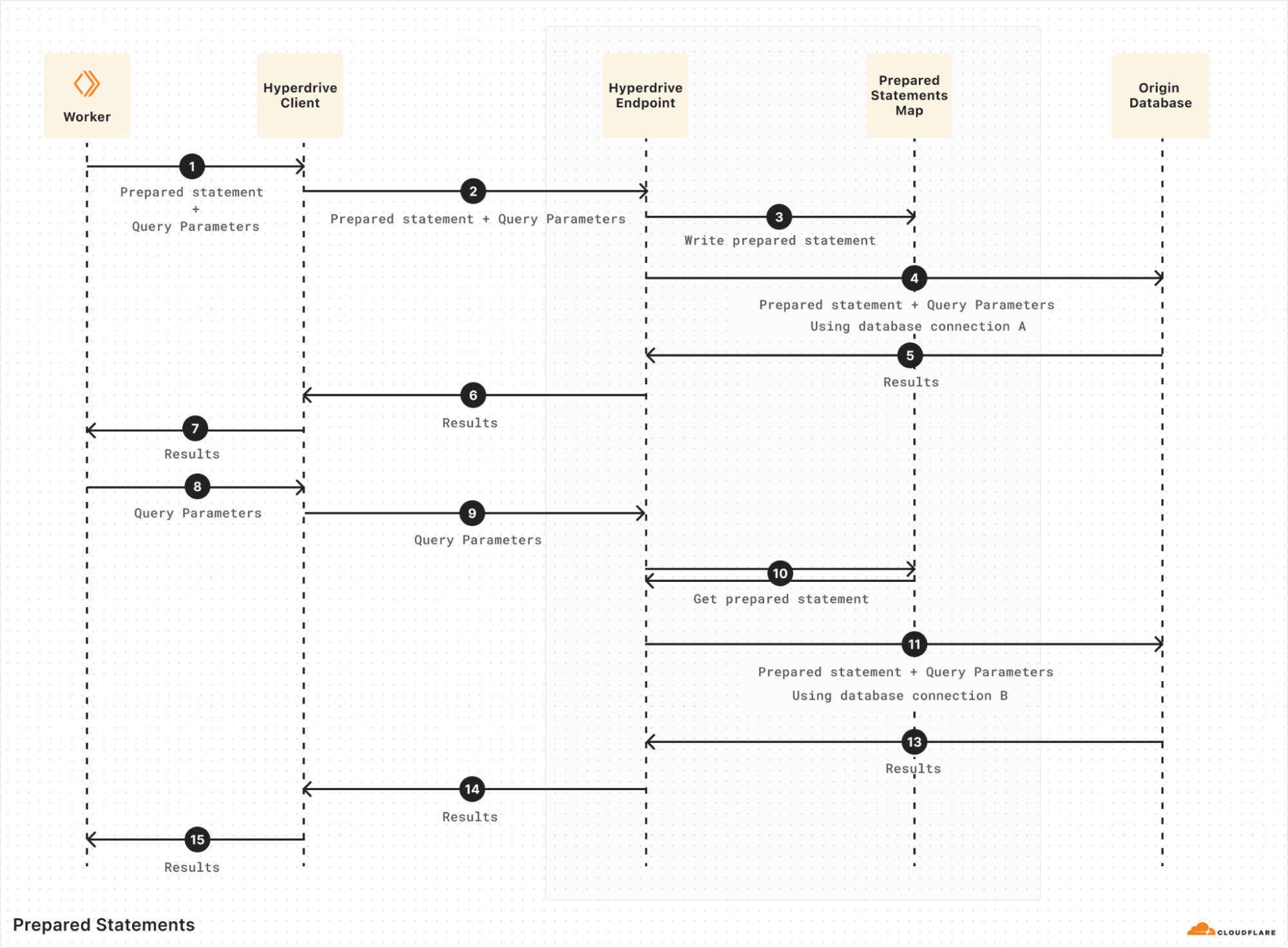
Hyperdrive implements this by keeping track of what statements have been prepared by a given client, as well as what statements have been prepared on each origin connection in the pool. When a query comes in expecting to re-use a particular prepared statement (#8 above), Hyperdrive checks if it’s been prepared on the checked-out origin connection. If it hasn’t, Hyperdrive will replay the wire-protocol message sequence to prepare it on the newly-checked-out origin connection (#10 above) before sending the query over it. Many little corrections like this are necessary to keep the client’s connection to Hyperdrive and Hyperdrive’s connection to the origin database lined up so that both sides see what they expect.
This “split connection” approach is the founding innovation of Hyperdrive, and one of the most vital aspects of it is how it affects starting up new connections. While the same 5+ round trips must always happen on startup, the actual time spent on the round trips can be dramatically reduced by conducting them over the smallest possible distances. This impact of distance can be so big that there is still a huge latency reduction even though the startup round trips must now happen twice (once each between the Worker and Client, and Endpoint and your origin database). So how do we decide where to run everything, to lean into that advantage as much as possible?
The placement of Client has not really changed since the original design of Hyperdrive. Sharing a server with the Worker sending the queries means that the Worker runtime can connect directly to Hyperdrive with no network hop needed. While there is always room for microoptimizations, it’s hard to do much better than that from an architecture perspective. By far the bigger piece of the latency puzzle is where to run Endpoint.
Hyperdrive keeps a list of data centers that are eligible to house Endpoints, requiring that they have sufficient capacity and the best routes available for pooled connections to use. The key challenge to overcome here is that a database connection string does not tell you where in the world a database actually is. The reality is that reliably going from a hostname to a precise (enough) geographic location is a hard problem, even leaving aside the additional complexity of doing so within a private network. So how do we pick from that list of eligible data centers?
For much of the time since its launch, Hyperdrive solved this with a regional pool approach. When a Worker connected to Hyperdrive, the location of the Worker was used to infer what region the end user was connecting from (e.g. ENAM, WEUR, APAC, etc. — see a rough breakdown here). Data centers to house Endpoints for any given Hyperdrive were deterministically selected from that region’s list of eligible options using rendezvous hashing, resulting in one pool of connections per region.
This approach worked well enough, but it had some severe shortcomings. The first and most obvious is that there’s no guarantee that the data center selected for a given region is actually closer to the origin database than the user making the request. This means that, while you’re getting the benefit of the excellent routing available on Cloudflare’s network, you may be going significantly out of your way to do so. The second downside is that, in the scenario where a new connection must be created, the round trips to do so may be happening over a significantly larger distance than is necessary if the origin database is in a different region than the Endpoint housing the regional connection pool. This increases latency and reduces throughput for the query that needs to instantiate the connection.
The final key downside here is an unfortunate interaction with Smart Placement, a feature of Cloudflare Workers that analyzes the duration of your Worker requests to identify the data center to run your Worker in. With regional Endpoints, the best Smart Placement can possibly do is to put your requests close to the Endpoint for whichever region the origin database is in. Again, there may be other data centers that are closer, but Smart Placement has no way to do better than where the Endpoint is because all Hyperdrive queries must route through it.
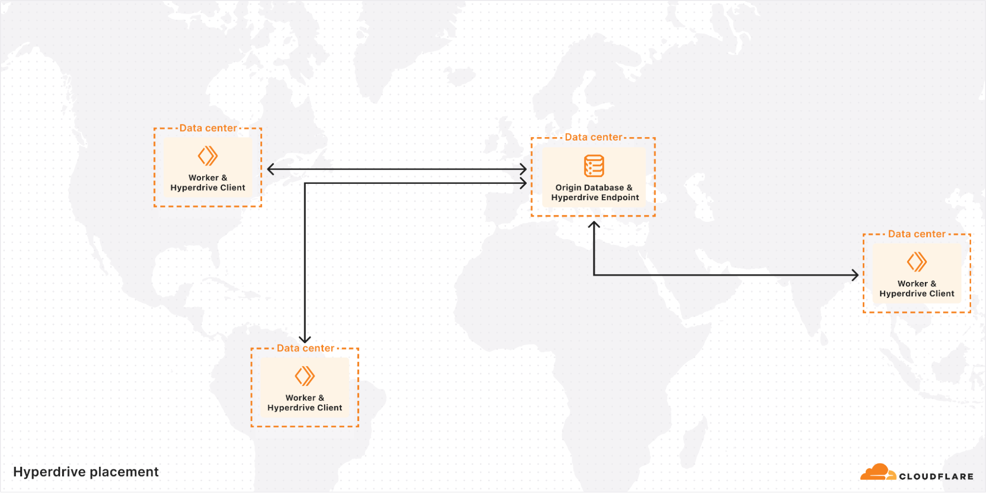
We recently shipped some improvements to this system that significantly enhanced performance. The new system discards the concept of regional pools entirely, in favor of a single global Endpoint for each Hyperdrive that is in the eligible data center as close as possible to the origin database.
The way we solved locating the origin database such that we can accomplish this was ultimately very straightforward. We already had a subsystem to confirm, at the time of creation, that Hyperdrive could connect to an origin database using the provided information. We call this subsystem our Edge Validator.
It’s bad user experience to allow someone to create a Hyperdrive, and then find out when they go to use it that they mistyped their password or something. Now they’re stuck trying to debug with extra layers in the way, with a Hyperdrive that can’t possibly work. Instead, whenever a Hyperdrive is created, the Edge Validator will send a request to an arbitrary data center to use its instance of Hyperdrive to connect to the origin database. If this connection fails, the creation of the Hyperdrive will also fail, giving immediate feedback to the user at the time it is most helpful.
With our new subsystem, affectionately called Placement, we now have a solution to the geolocation problem. After Edge Validator has confirmed that the provided information works and the Hyperdrive is created, an extra step is run in the background. Placement will perform the exact same connection routine, except instead of being done once from an arbitrary data center, it is run a handful of times from every single data center that is eligible to house Endpoints. The latency of establishing these connections is collected, and the average is sent back to a central instance of Placement. The data centers that can connect to the origin database the fastest are, by definition, where we want to run Endpoint for this Hyperdrive. The list of these is saved, and at runtime is used to select the Endpoint best suited to housing the pool of connections to the origin database.
Given that the secret sauce of Hyperdrive is in managing and minimizing the latency of establishing these connections, moving Endpoints right next to their origin databases proved to be pretty impactful.
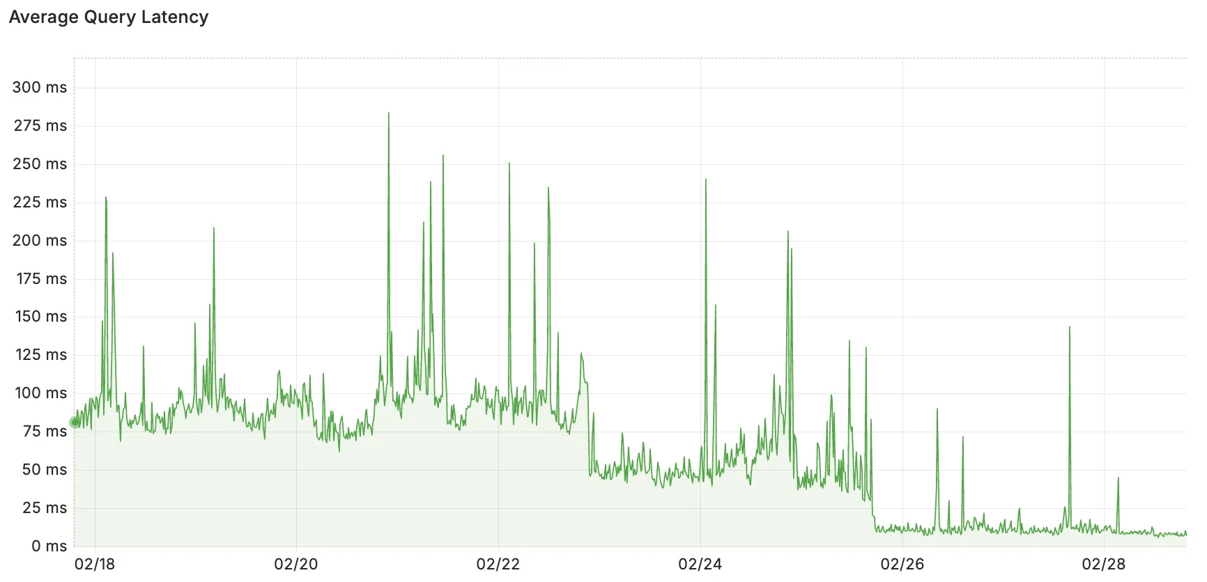
Pictured: query latency as measured from Endpoint to origin databases. The backfill of Placement to existing customers was done in stages on 02/22 and 02/25.
While we went in a different direction, it’s worth acknowledging that other teams have solved this same problem with a very different approach. Custom database drivers, usually called “serverless drivers”, have made several optimization efforts to reduce both the number of round trips and how quickly they can be conducted, while still connecting directly from your client to your database in the traditional way. While these drivers are impressive, we chose not to go this route for a couple of reasons.
First off, a big part of the appeal of using Postgres is its vibrant ecosystem. Odds are good you’ve used Postgres before, and it can probably help solve whichever problem you’re tackling with your newest project. This familiarity and shared knowledge across projects is an absolute superpower. We wanted to lean into this advantage by supporting the most popular drivers already in this ecosystem, instead of fragmenting it by adding a competing one.
Second, Hyperdrive also functions as a cache for individual queries (a bit of trivia: its name while still in Alpha was actually sql-query-cache). Doing this as effectively as possible for distributed users requires some clever positioning of where exactly the query results should be cached. One of the unique advantages of running a distributed service on Cloudflare’s network is that we have a lot of flexibility on where to run things, and can confidently surmount challenges like those. If we’re going to be playing three-card monte with where things are happening anyway, it makes the most sense to favor that route for solving the other problems we’re trying to tackle too.
As we’ve talked about in the past, Hyperdrive buffers protocol messages until it has enough information to know whether a query can be served from cache. In a post about how Hyperdrive works it would be a shame to skip talking about how exactly we cache query results, so let’s close by diving into that.
First and foremost, Hyperdrive uses Cloudflare’s cache, because when you have technology like that already available to you, it’d be silly not to use it. This has some implications for our architecture that are worth exploring.
The cache exists in each of Cloudflare’s data centers, and by default these are separate instances. That means that a Client operating close to the user has one, and an Endpoint operating close to the origin database has one. However, historically we weren’t able to take full advantage of that, because the logic for interacting with cache was tightly bound to the logic for managing the pool of connections.
Part of our recent architecture refactoring effort, where we switched to global Endpoints, was to split up this logic such that we can take advantage of Client’s cache too. This was necessary because, with Endpoint moving to a single location for each Hyperdrive, users from other regions would otherwise have gotten cache hits served from almost as far away as the origin.
With the new architecture, the role of Client during active query handling transitioned from that of a “dumb pipe” to more like what Endpoint had always been doing. It now buffers protocol messages, and serves results from cache if possible. In those scenarios, Hyperdrive’s traffic never leaves the data center that the Worker is running in, reducing query latencies from 20-70 ms to an average of around 4 ms. As a side benefit, it also substantially reduces the network bandwidth Hyperdrive uses to serve these queries. A win-win!
In the scenarios where query results can’t be served from the cache in Client’s data center, all is still not lost. Endpoint may also have cached results for this query, because it can field traffic from many different Clients around the world. If so, it will provide these results back to Client, along with how much time is remaining before they expire, such that Client can both return them and store them correctly into its own cache. Likewise, if Endpoint does need to go to the origin database for results, they will be stored into both Client and Endpoint caches. This ensures that followup queries from that same Client data center will get the happy path with single-digit ms response times, and also reduce load on the origin database from any other Client’s queries. This functions similarly to how Cloudflare’s Tiered Cache works, with Endpoint’s cache functioning as a final layer of shielding for the origin database.
With this announcement of a Free Plan for Hyperdrive, and newly armed with the knowledge of how it works under the hood, we hope you’ll enjoy building your next project with it! You can get started with a single Wrangler command (or using the dashboard):
wrangler hyperdrive create postgres-hyperdrive
--connection-string="postgres://user:[email protected]:5432/defaultdb"
We’ve also included a Deploy to Cloudflare button below to let you get started with a sample Worker app using Hyperdrive, just bring your existing Postgres database! If you have any questions or ideas for future improvements, please feel free to visit our Discord channel!
Post Syndicated from Korinne Alpers original https://blog.cloudflare.com/full-stack-development-on-cloudflare-workers/
In September 2024, we introduced beta support for hosting, storing, and serving static assets for free on Cloudflare Workers — something that was previously only possible on Cloudflare Pages. Being able to host these assets — your client-side JavaScript, HTML, CSS, fonts, and images — was a critical missing piece for developers looking to build a full-stack application within a single Worker.
Today we’re announcing ten big improvements to building apps on Cloudflare. All together, these new additions allow you to build and host projects ranging from simple static sites to full-stack applications, all on Cloudflare Workers:
Cloudflare Workers now provides production ready, generally available (GA) support for React Router v7 (Remix), Astro, Hono, Vue.js, Nuxt, Svelte (SvelteKit), and more, with GA support for more frameworks including Next.js, Angular, and SolidJS (SolidStart) to follow in Q2 2025.
You can build complete full-stack apps on Workers without a framework: you can “just use Vite” and React together, and build a backend API in the same Worker. See our Vite + React template for an example.
The adapter for Next.js — @opennextjs/cloudflare, introduced in September 2024 as an early alpha, is now v1.0-beta, and will be GA in the coming weeks. Those using the OpenNext adapter will also be able to easily upgrade to the recently announced Next.js Deployments API.
The Cloudflare Vite plugin is now v1.0 and generally available. The Vite plugin allows you to run Vite’s development server in the Workers runtime (workerd), meaning you get all the benefits of Vite, including Hot Module Replacement, while still being able to use features that are exclusive to Workers (like Durable Objects).
You can now use static _headers and _redirects configuration files for your applications on Workers, something that was previously only available on Pages. These files allow you to add simple headers and configure redirects without executing any Worker code.
In addition to PostgreSQL, you can now connect to MySQL databases in addition from Cloudflare Workers, via Hyperdrive. Bring your existing Planetscale, AWS, GCP, Azure, or other MySQL database, and Hyperdrive will take care of pooling connections to your database and eliminating unnecessary roundtrips by caching queries.
More Node.js APIs are available in the Workers Runtime — including APIs from the crypto, tls, net, and dns modules. We’ve also increased the maximum CPU time for a Workers request from 30 seconds to 5 minutes.
You can now bring any repository from GitHub or GitLab that contains a Worker application, and Workers Builds will take care of deploying the app as a new Worker on your account. Workers Builds is also starting much more quickly (by up to 6 seconds for every build).
You can now set up Workers Builds to run on non-production branches, and preview URLs will be posted back to GitHub as a comment.
The Images binding in Workers is generally available, allowing you to build more flexible, programmatic workflows.
These improvements allow you to build both simple static sites and more complex server-side rendered applications. Like Pages, you only get charged when your Worker code runs, meaning you can host and serve static sites for free. When you want to do any rendering on the server or need to build an API, simply add a Worker to handle your backend. And when you need to read or write data in your app, you can connect to an existing database with Hyperdrive, or use any of our storage solutions: Workers KV, R2, Durable Objects, or D1.
If you’d like to dive straight into code, you can deploy a single-page application built with Vite and React, with the option to connect to a hosted database with Hyperdrive, by clicking this “Deploy to Cloudflare” button:
Previously, you needed to choose between building on Cloudflare Pages or Workers (or use Pages for one part of your app, and Workers for another) just to get started. This meant figuring out what your app needed from the start, and hoping that if your project evolved, you wouldn’t be stuck with the wrong platform and architecture. Workers was designed to be a flexible platform, allowing developers to evolve projects as needed — and so, we’ve worked to bring pieces of Pages into Workers over the years.
Now that Workers supports both serving static assets and server-side rendering, you should start with Workers. Cloudflare Pages will continue to be supported, but, going forward, all of our investment, optimizations, and feature work will be dedicated to improving Workers. We aim to make Workers the best platform for building full-stack apps, building upon your feedback of what went well with Pages and what we could improve.
Before, building an app on Pages meant you got a really easy, opinionated on-ramp, but you’d eventually hit a wall if your application got more complex. If you wanted to use Durable Objects to manage state, you would need to set up an entirely separate Worker to do so, ending up with a complicated deployment and more overhead. You also were limited to real-time logs, and could only roll out changes all in one go.
When you build on Workers, you can immediately bind to any other Developer Platform service (including Durable Objects, Email Workers, and more), and manage both your front end and back end in a single project — all with a single deployment. You also get the whole suite of Workers observability tooling built into the platform, such as Workers Logs. And if you want to rollout changes to only a certain percentage of traffic, you can do so with Gradual Deployments.
These latest improvements are part of our goal to bring the best parts of Pages into Workers. For example, we now support static _headers and _redirects config files, so that you can easily take an existing project from Pages (or another platform) and move it over to Workers, without needing to change your project. We also directly integrate with GitHub and GitLab with Workers Builds, providing automatic builds and deployments. And starting today, Preview URLs are posted back to your repository as a comment, with feature branch aliases and environments coming soon.
To learn how to migrate an existing project from Pages to Workers, read our migration guide.
Next, let’s talk about how you can build applications with different rendering modes on Workers.
As a quick primer, here are all the architectures and rendering modes we’ll be discussing that are supported on Workers:
Static sites: When you visit a static site, the server immediately returns pre-built static assets — HTML, CSS, JavaScript, images, and fonts. There’s no dynamic rendering happening on the server at request-time. Static assets are typically generated at build-time and served directly from a CDN, making static sites fast and easily cacheable. This approach works well for sites with content that rarely changes.
Single-Page Applications (SPAs): When you load an SPA, the server initially sends a minimal HTML shell and a JavaScript bundle (served as static assets). Your browser downloads this JavaScript, which then takes over to render the entire user interface client-side. After the initial load, all navigation occurs without full-page refreshes, typically via client-side routing. This creates a fast, app-like experience.
Server-Side Rendered (SSR) applications: When you first visit a site that uses SSR, the server generates a fully-rendered HTML page on-demand for that request. Your browser immediately displays this complete HTML, resulting in a fast first page load. Once loaded, JavaScript “hydrates” the page, adding interactivity. Subsequent navigations can either trigger new server-rendered pages or, in many modern frameworks, transition into client-side rendering similar to an SPA.
Next, we’ll dive into how you can build these kinds of applications on Workers, starting with setting up your development environment.
Before uploading your application, you need to bundle all of your client-side code into a directory of static assets. Wrangler bundles and builds your code when you run wrangler dev, but we also now support Vite with our new Vite plugin. This is a great option for those already using Vite’s build tooling and development server — you can continue developing (and testing with Vitest) using Vite’s development server, all using the Workers runtime.
To get started using the Cloudflare Vite plugin, you can scaffold a React application using Vite and our plugin, by running:
npm create cloudflare@latest my-react-app -- --framework=reactWhen you open the project, you should see a directory structure like this:
...
├── api
│   └── index.ts
├── public
│   └── ...
├── src
│   └── ...
...
├── index.html
├── package.json
├── vite.config.ts
└── wrangler.jsonc
If you run npm run build, you’ll see a new folder appear, named /dist.
...
├── api
│   └── index.ts
├── dist
│   └── ...
├── public
│   └── ...
├── src
│   └── ...
...
├── index.html
├── package.json
├── vite.config.ts
└── wrangler.jsonc
The Vite plugin informs Wrangler that this /dist directory contains the project’s built static assets — which, in this case, includes client-side code, some CSS files, and images.
Once deployed, this single-page application (SPA) architecture will look something like this:
When a request comes in, Cloudflare looks at the pathname and automatically serves any static assets that match that pathname. For example, if your static assets directory includes a blog.html file, requests for example.com/blog get that file.
If you have a static site created by a static site generator (SSG) like Astro, all you need to do is create a wrangler.jsonc file (or wrangler.toml) and tell Cloudflare where to find your built assets:
// wrangler.jsonc

{
  "name": "my-static-site",
  "compatibility_date": "2025-04-01",
  "assets": {
    "directory": "./dist",
  }
}
Once you’ve added this configuration, you can simply build your project and run wrangler deploy. Your entire site will then be uploaded and ready for traffic on Workers. Once deployed and requests start flowing in, your static site will be cached across Cloudflare’s network.
You can try starting a fresh Astro project on Workers today by running:
npm create cloudflare@latest my-astro-app -- --framework=astroYou can see our other supported Frameworks and how to get started in our framework guides.
If you have a single-page application, you can explicitly enable single-page-application mode in your Wrangler configuration:
{
 "name": "example-spa-worker-hyperdrive",
 "main": "api/index.js",
 "compatibility_flags": ["nodejs_compat"],
 "compatibility_date": "2025-04-01",
 },
 "assets": {
   "directory": "./dist",
   "binding": "ASSETS",
   "not_found_handling": "single-page-application"
 },
 "hyperdrive": [
   {
     "binding": "HYPERDRIVE",
     "id": "d9c9cfb2587f44ee9b0730baa692ffec",
     "localConnectionString": "postgresql://myuser:mypassword@localhost:5432/mydatabase"
   }
 ],
 "placement": {
   "mode": "smart"
 }
}
By enabling this, the platform assumes that any navigation request (requests which include a Sec-Fetch-Mode: navigate header) are intended for static assets and will serve up index.html whenever a matching static asset match cannot be found. For non-navigation requests (such as requests for data) that don’t match a static asset, Cloudflare will invoke the Worker script. With this setup, you can render the frontend with React, use a Worker to handle back-end operations, and use Vite to help stitch the two together. This is a great option for porting over older SPAs built with create-react-app, which was recently sunset.
Another thing to note in this Wrangler configuration file: we’ve defined a Hyperdrive binding and enabled Smart Placement. Hyperdrive lets us use an existing database and handles connection pooling. This solves a long-standing challenge of connecting Workers (which run in a highly distributed, serverless environment) directly to traditional databases. By design, Workers operate in lightweight V8 isolates with no persistent TCP sockets and a strict CPU/memory limit. This isolation is great for security and speed, but it makes it difficult to hold open database connections. Hyperdrive addresses these constraints by acting as a “bridge” between Cloudflare’s network and your database, taking care of the heavy lifting of maintaining stable connections or pools so that Workers can reuse them. By turning on Smart Placement, we also ensure that if requests to our Worker originate far from the database (causing latency), Cloudflare can choose to relocate both the Worker—which handles the database connection—and the Hyperdrive “bridge” to a location closer to the database, reducing round-trip times.
Let’s look at the “Deploy to Cloudflare” example at the top of this blog. In api/index.js, we’ve defined an API (using Hono) which connects to a hosted database through Hyperdrive.
import { Hono } from "hono";
import postgres from "postgres";
import booksRouter from "./routes/books";
import bookRelatedRouter from "./routes/book-related";

const app = new Hono();

// Setup SQL client middleware
app.use("*", async (c, next) => {
 // Create SQL client
 const sql = postgres(c.env.HYPERDRIVE.connectionString, {
   max: 5,
   fetch_types: false,
 });

 c.env.SQL = sql;

 // Process the request
 await next();

 // Close the SQL connection after the response is sent
 c.executionCtx.waitUntil(sql.end());
});

app.route("/api/books", booksRouter);
app.route("/api/books/:id/related", bookRelatedRouter);


export default {
 fetch: app.fetch,
};
When deployed, our app’s architecture looks something like this:
If Smart Placement moves the placement of my Worker to run closer to my database, it could look like this:
If you want to handle rendering on the server, we support a number of popular full-stack frameworks.
Here’s a version of our previous example, now using React Router v7’s server-side rendering:
You could also use Next.js with the OpenNext adapter, or any other framework listed in our framework guides.
We’ve also continued to make progress supporting Node.js APIs, recently adding support for the crypto, tls, net, and dns modules. This allows existing applications and libraries that rely on these Node.js modules to run on Workers. Let’s take a look at an example:
Previously, if you tried to use the mongodb package, you encountered the following error:
Error: [unenv] dns.resolveTxt is not implemented yet!This occurred when mongodb used the node:dns module to do a DNS lookup of a hostname. Even if you avoided that issue, you would have encountered another error when mongodb tried to use node:tls to securely connect to a database.
Now, you can use mongodb as expected because node:dns and node:tls are supported. The same can be said for libraries relying on node:crypto and node:net.
Additionally, Workers now expose environment variables and secrets on the process.env object when the nodejs_compat compatibility flag is on and the compatibility date is set to 2025-04-01 or beyond. Some libraries (and developers) assume that this object will be populated with variables, and rely on it for top-level configuration. Without the tweak, libraries may have previously broken unexpectedly and developers had to write additional logic to handle variables on Cloudflare Workers.
Now, you can just access your variables as you would in Node.js.
const LOG_LEVEL = process.env.LOG_LEVEL || "info";We have also raised the maximum CPU time per Worker request from 30 seconds to 5 minutes. This allows for compute-intensive operations to run for longer without timing out. Say you want to use the newly supported node:crypto module to hash a very large file, you can now do this on Workers without having to rely on external compute for CPU-intensive operations.
We’ve also made improvements to Workers Builds, which allows you to connect a Git repository to your Worker, so that you can have automatic builds and deployments on every pushed change. Workers Builds was introduced during Builder Day 2024, and initially only allowed you to connect a repository to an existing Worker. Now, you can bring a repository and immediately deploy it as a new Worker, reducing the amount of setup and button clicking needed to bring a project over. We’ve improved the performance of Workers Builds by reducing the latency of build starts by 6 seconds — they now start within 10 seconds on average. We also boosted API responsiveness, achieving a 7x latency improvement thanks to Smart Placement.
Note: On April 2, 2025, Workers Builds transitioned to a new pricing model, as announced during Builder Day 2024. Free plan users are now capped at 3,000 minutes of build time, and Workers Paid subscription users will have a new usage-based model with 6,000 free minutes included and $0.005 per build minute pricing after. To better support concurrent builds, Paid plans will also now get six (6) concurrent builds, making it easier to work across multiple projects and monorepos. For more information on pricing, see the documentation.
You can also set up Workers Builds to run on non-production branches, and preview URLs will be posted back to GitHub as a comment.
Last week, we wrote a blog post that covers how the Images binding enables more flexible, programmatic workflows for image optimization.
Previously, you could access image optimization features by calling fetch() in your Worker. This method requires the original image to be retrievable by URL. However, you may have cases where images aren’t accessible from a URL, like when you want to compress user-uploaded images before they are uploaded to your storage. With the Images binding, you can directly optimize an image by operating on its body as a stream of bytes.
To learn more, read our guide on transforming an image before it gets uploaded to R2.
We’re excited to see what you’ll build, and are focused on new features and improvements to make it easier to create any application on Workers. Much of this work was made even better by community feedback, and we encourage everyone to join our Discord to participate in the discussion.
Helpful resources to get you started: