There was something of a space theme that pervaded the Embedded Linux
Conference (ELC) portion of the 2023 Embedded
Open Source Summit (EOSS), which is an umbrella event for various
sub-conferences related to embedded open-source development. That may
partly be because one of the organizers of EOSS (and ELC), Tim Bird,
described himself as “a bit of a space junkie”; he made that observation
during a panel session that he led on embedded Linux in space. Bird and
four panelists discussed various aspects of the use of Linux in
space-related systems, including where it has been used, the
characteristics and challenges of aerospace deployments, certification of
Linux for aerospace use, and more.
Security updates have been issued by Debian (python-git and renderdoc), Red Hat (edk2, kernel, kernel-rt, and kpatch-patch), Slackware (kernel), SUSE (firefox, libcap, openssh, openssl-1_1, python39, and zabbix), and Ubuntu (cinder, ironic, nova, python-glance-store, python-os-brick, frr, graphite-web, and openssh).
The details are scant—the article is based on a “heavily redacted” contract—but the New York subway authority is using an “AI system” to detect people who don’t pay the subway fare.
Joana Flores, an MTA spokesperson, said the AI system doesn’t flag fare evaders to New York police, but she declined to comment on whether that policy could change. A police spokesperson declined to comment.
If we spent just one-tenth of the effort we spend prosecuting the poor on prosecuting the rich, it would be a very different world.
22 май 2023 г. Налагаше се да бъда в движение из града през почти целия ден, а в същото време трябваше да поддържам активна комуникация по телефона и в чата с колегите по различни теми и проекти. Всичко щеше да бъде наред, ако изведнъж в късния следобед телефоните им не замлъкнаха. Нямах телефонна връзка и с никого от мениджмънта на компанията. Намерихме се чрез служебния чат, където стана ясно, че мобилният оператор „А1 България“ едностранно и без да посочи конкретна причина, просто е спрял телефоните на всички, включени в групата на фирмата.
Над два месеца по-късно проблемът още няма решение, нито пък от А1 са дали рационално обяснение, в което да не прозира опит за натиск от позицията на силата. Разпитвайки наоколо, попаднах и на други подобни случаи, което предполага, че
всичко това може би не е случайно, а прилича на установена търговска практика.
Заех се да пиша този текст по няколко причини. Като служител на една от засегнатите компании имах възможност да наблюдавам развоя на казуса съвсем отблизо. Освен това, разравяйки фактите, попаднах на стряскащо идентични случаи с други дългогодишни клиенти на мобилния оператор. А съм наясно, че тъй като телекомите са едни от най-големите рекламодатели, примери за техни скандални практики трудно ще получат отразяване в по-големите медии.
Случаят с „Новарто“
„Новарто“ е българска ИТ компания, която от 15 години е клиент на „A1 България“. Досега двете дружества не са имали никакви юридически или други спорове.
Тази година ръководството на „Новарто“ решава да смени мобилния оператор, вместо да поднови договора си с А1. Фирмата подготвя заявлението за пренос на номерата, но изчаква да наближи крайният срок на договора, който изтича на 4 юни. Междувременно от „Новарто“ споделят с обслужващия търговец на А1, че разглеждат и други оферти.
На 22 май в 16:09 ч. управителят на „Новарто“ Борислав Минков получава имейл от Димитър С. Димитров, мениджър „Големи клиенти“ в „A1 България“. Той го уведомява, че считано от същия ден, договорът за мобилните услуги се прекратява едностранно от телекома на основание Раздел 9 от Общите условия на „А1 България“. Петдесет и девет минути по-късно, в 17:08 ч., всички SIM карти от фирмената група на „Новарто“ се превръщат в непотребни парченца пластмаса. А служителите заедно с мениджърите на компанията остават недостъпни по телефона за колегите, клиентите и бизнес партньорите си, както и за семействата и приятелите си.
Цитираният Раздел 9 от Общите условия на „А1 България“, разписан в над две страници, обхваща всички различни хипотези, при които договорът за мобилни услуги може да бъде прекратен от клиента или от оператора. Иначе казано, в позоваването на целия раздел няма полезна конкретика, която да изясни
защо едностранно и с едночасово предизвестие се прекратява договор, който фактически не е изтекъл.
При това развитие „Новарто“ изисква от новия си мобилен оператор да задейства веднага подготвеното заявление за пренос на номерата. За съжаление, това се оказва закъснял ход – наближава краят на работното време, а на следващия ден A1 отказва преноса, обосновавайки се с прекратения договор заради нарушени Общи условия.
Обичайната процедура за пренос на номера от един телеком към друг изисква клиентът да заяви това при новия си оператор, който служебно препраща заявката към стария. Той от своя страна следва да уведоми клиента си, че номерът или номерата му са заявени за пренос (прави се, за да се избегнат евентуални опити за злоупотреба) и че може да дължи някакви неустойки (за предсрочно прекратяване на договора, за невърнати устройства и др.). Обикновено преносът се осъществява в рамките на няколко дни.
В конкретния случай старият оператор („A1 България“) предсрочно прекратява договора, изпреварвайки заявлението за пренос.
Така, когато такова заявление постъпи, той вече може да твърди, че клиентът няма активен договор, и на това основание да откаже преноса. Негативният ефект е двоен – клиентът остава без комуникации за неопределен период, а същевременно не може да премести номерата си към друг оператор.
Представете си, че сте търговска фирма, която приема поръчки по телефона, и в един момент никой не може да се свърже с вас. А дори да вземете нови телефонни номера, имате стотици клиенти, които трябва да уведомите за това. Или както споделя Борислав Минков, телефонът или имейлът само на пръв поглед са някаква поредица от букви и цифри, а в действителност са жива връзка с бизнес партньорите ти. Когато някой ти отнеме тази връзка, той не просто възпрепятства бизнеса ти, а ограничава човешкото ти общуване – защото зад всеки телефонен номер всъщност стои човек.
Юридически доказването на вреди и пропуснати ползи е трудно упражнение, но Минков добавя и втори план за размисъл, защото, случайно или не,
както „A1 България“, така и „Новарто“ са партньори на немския софтуерен гигант SAP – и в този смисъл се явяват конкуренти.
Факт, за който Минков се надява, че ще заинтересува Комисията за защита на конкуренцията.
Жалба от страна на „Новарто“ е подадена също в Комисията за регулиране на съобщенията, изпратено е и писмо до оглавяващия отдела за вътрешен одит в Telekom Austria Group – компанията майка на „A1 България“.
От името на „Тоест“ се обърнах към г-жа Илияна Захариева, директор „Корпоративни комуникации“, със следните въпроси:
Каква е причината за едностранното предсрочно прекратяване на услугите по упоменатия договор с „Новарто“ ООД?
Счита ли „А1 България“ за добра търговска практика едностранното предсрочно прекратяване на услуги по действащ договор, без детайлно и аргументирано посочване на причина за това?
Как ще коментирате страничния ефект на това едностранно предсрочно прекратяване, който води до невъзможност клиентът Ви да ползва услугите от Вас, нито да може да пренесе номерата си при друг мобилен оператор?
Г-жа Захариева не отговори на въпросите ми, но потвърди, че от „A1 България“ са запознати със случая, който тя определи като частен казус, и обясни, че поради тази причина не може да коментира детайли, без да сподели данни за сметките, задълженията и транзакциите на „Новарто“. Тя повтори, че договорът е прекратен едностранно, на основание нарушаване на Общите условия – отново без друга конкретика.
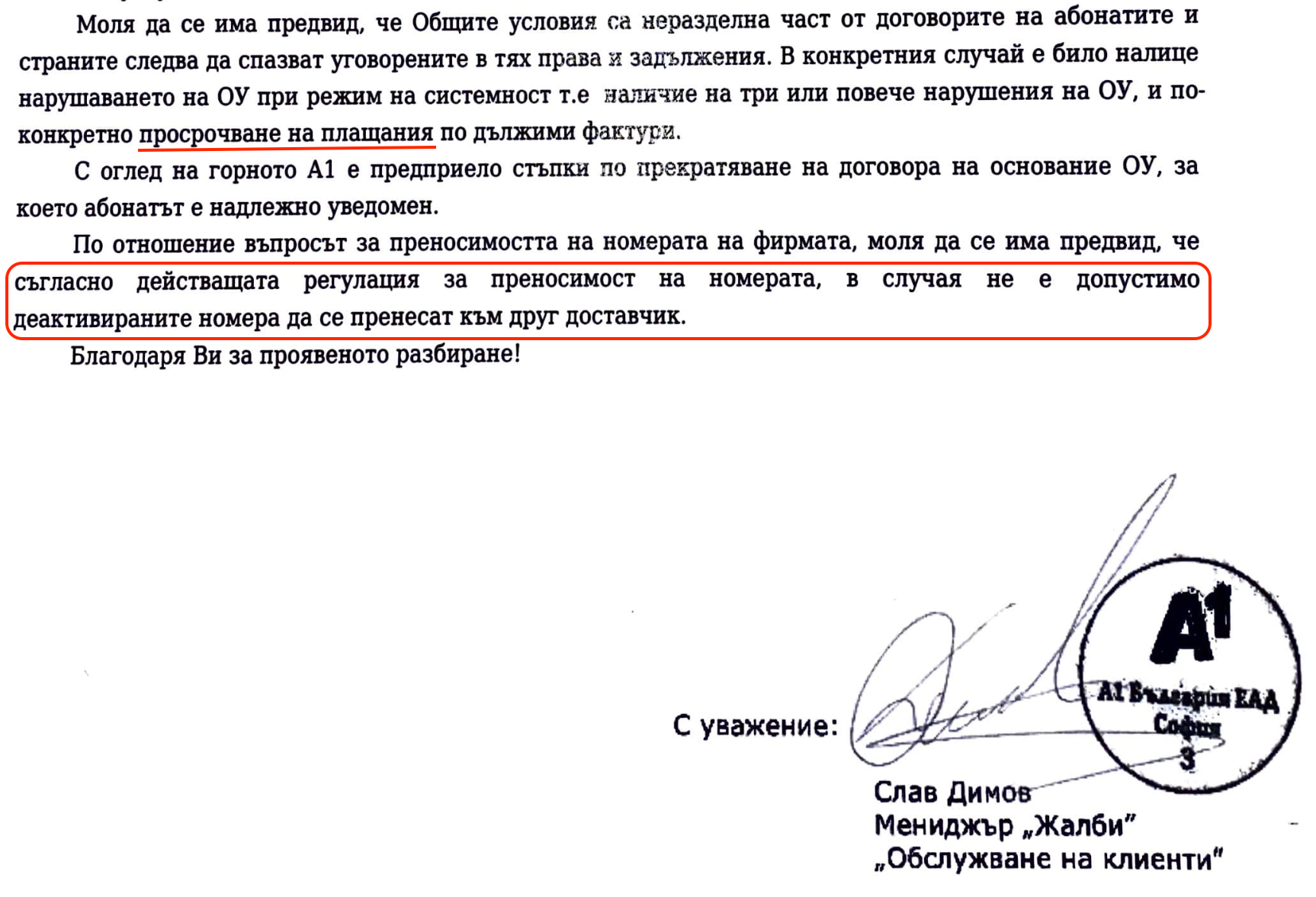
Официалната позиция по случая от страна на „A1 България“, получена над месец след жалбата на „Новарто“, повтаря за пореден път всичко известно дотук. Добавен е обаче един детайл. Операторът претендира, че компанията „Новарто“ поне три пъти е просрочила плащания на дължими фактури.
Борислав Минков не отрича, че е открил няколко фактури, на които „Новарто“ е просрочила плащанията, но е категоричен, че са били неволни забавяния с не повече от два-три дни, а не системно поведение. И това е за целия период от 15 години, през които двете компании са имали търговски взаимоотношения. Минков задава и следния очевиден въпрос:
Ако това е било системно нарушение от наша страна, защо A1 никога не са реагирали? Защо досега не са прекратили отношенията си с нас, а го правят едва когато научиха, че ще ги сменим?
Междувременно в конферентен разговор с въпросния мениджър „Големи клиенти“ Димитър С. Димитров и с регионалния мениджър Иван С. Иванов, проведен в първите дни след прекратяването на договора, Минков получава предложение „да преподпише с A1 и да забравят за случилото се“. Или „да компенсира A1 с друг двугодишен договор, който да им възстанови загубения оборот“. Той отказва.
В крайна сметка „Новарто“ подписва нов договор с друг оператор, прежалвайки старите си номера. Това, естествено, води до сътресения в бизнеса и комуникациите, докато всички контрагенти научат новите телефонни номера на служителите, които работят с тях. Процесът отнема време и не е лесен.
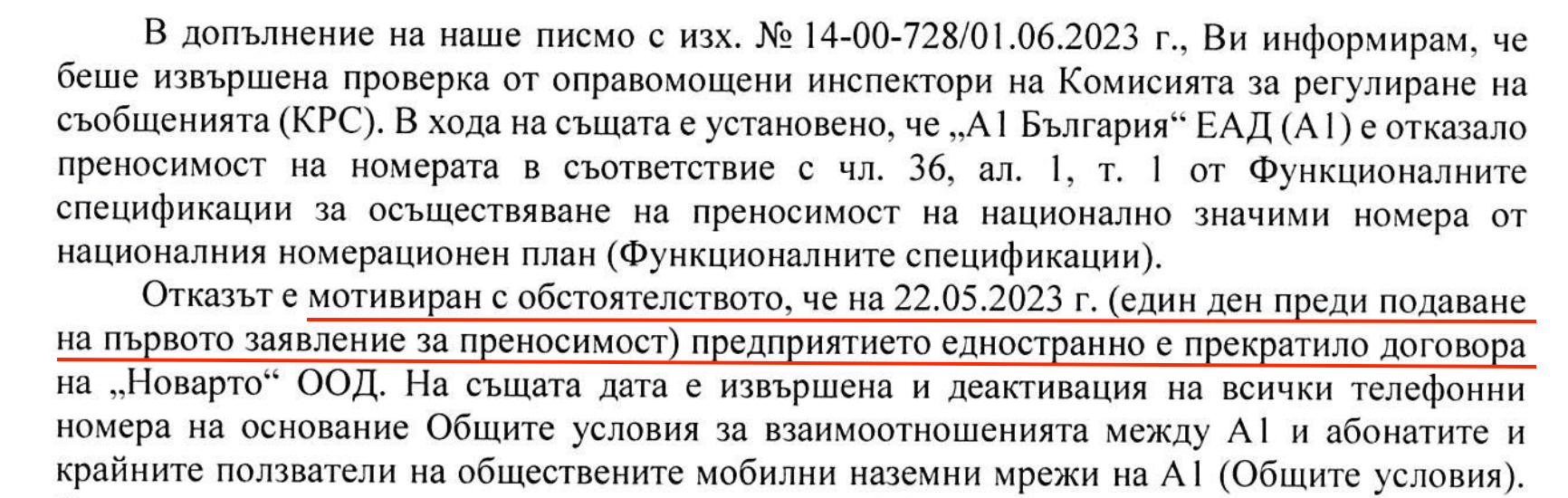
На 7 юли „Новарто“ получава отговор и на жалбата си до Комисията за регулиране на съобщенията, която заявява, че „A1 България“ е отказала преноса на номерата в съответствие с регулаторните изисквания (чл. 36, ал. 1, т. 1 от Функционалните спецификации), тъй като преди подаване на заявлението за преносимост номерата са били деактивирани, тоест несъществуващи.
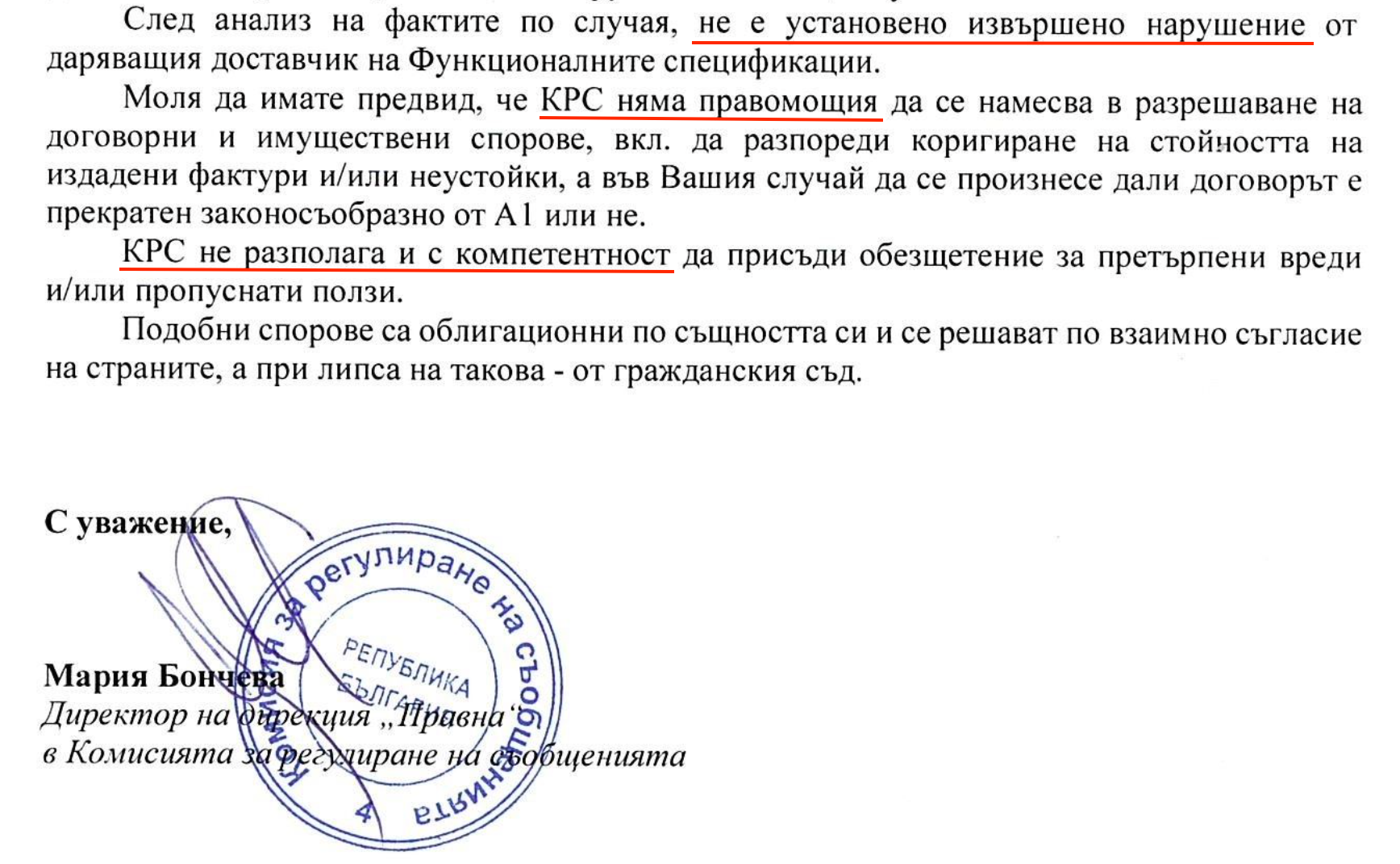
КРС подчертава и че „няма правомощия да се намесва в разрешаване на договорни и имуществени спорове“, а в конкретния случай – „да се произнесе дали договорът е прекратен законосъобразно от A1, или не“.
Дали от „A1 България“ не разчитат именно на това?
Те формално изпълняват регулаторните изисквания, но си позволяват търговски практики, граничещи с изнудване, защото разчитат, че клиентите им ще се огънат, осъзнавайки колко трудно ще е да защитят правата си, освен по съдебен път. Въпреки че това е скъп и бавен процес, Борислав Минков е категоричен, че ще съди „A1 България“. И не е сам в това си намерение.
И още от същото
Месец след случая с „Новарто“ разговарям с Николай Александриев, управител на транспортната компания „Никми Транс“, и историята, която той споделя, е сякаш копирана под индиго. По думите му, неговата фирма е клиент на „A1 България“ от поне 15 години и никога през това време не са имали нагласата да сменят своя мобилен оператор. Александриев твърди, че месечните им сметки към A1 са били между 2500 и 3500 лв., което включва услуги за мобилна телефония, интернет, телевизия и GPS контрол на превозните им средства.
С годините обаче договорът им с А1 започва да изглежда все по-неизгоден, особено в сравнение с предложенията на други телекоми. „И въпреки това – споделя с мен Николай Александриев – аз им казах, че не искам да сменям оператора, а искам да ми предложат това, което бих получил другаде.“ Обещават му го, но връщат проектодоговор, в който това не личи. „Дадох го на мои служители да го прочетат, да не би аз нещо да пропускам“, отбелязва Александриев с неприкрита ирония.
Обажда им се, че предложението не е каквото е очаквал, провеждат среща в офиса му на 26 юни, около 16 ч., и получава уверения от своя акаунт мениджър, че ще говорят отново на следващия ден. На 27 юни обаче, в 9:02 ч., Александриев получава SMS, че всички договори и услуги се прекратяват едностранно от „А1 България“.
Камионите ми са по Европа и останах без комуникация с шофьорите. Добре че повечето имаха и лични телефони. Обадих се от друг телефон на акаунт мениджъра ни Стоян, който ми обясни, че причината за прекратяването е, защото не сме подписали договора. Майка ми, която е служителка във фирмата, също го намира по Viber и той ѝ казва същото: „Подпишете си договора и веднага ще ви бъдат пуснати услугите.“
„Договорът ви беше ли вече изтекъл?“, питам г-н Александриев. „Да, беше изтекъл, но имам клауза, според която той се превръща в безсрочен, а не се прекратява.“ Питам го и дали има официално становище все пак на какво основание операторът прави това. „Поради неплатени фактури – отговаря той, – но срокът ми за плащане е до 29 юни, а това се случва на 27-ми.“
Разговорът ни приключва с категорична декларация от негова страна, че ще води дело срещу „А1 България“.
Докато разнищвах двата случая, се запознах и с друг човек, вече пенсионер, оттеглил се от бизнеса, но преди две-три години преминал през много подобна ситуация. Неговият разказ потвърждава, че
тези практики на „А1 България“ не са нови.
Разговарях с Кирил Паскалев по телефона, а случаят е свързан с фирмата, която е представлявал – „Майнинг Конструкшън Къмпани“. Един ден услугите, които „A1 България“ предоставя на компанията, са спрени, а на Паскалев му е обяснено, че ще бъдат подновени само ако преподпише нов договор с нови условия. Те са по-неизгодни от тези, на които фирмата му е била досега. Паскалев подписва договора, за да спаси номерата си, и веднага след като услугите са възстановени, подава искане за пренос към друг оператор, след което плаща и неустойка на „A1 България“ за прекратения толкова скоро нов договор. Откупил се скъпо, но за фирмата било много важно да запази номерата, с които е известна на клиентите си.
Задънена улица
Успях да стигна до тези няколко случая без особени усилия. Имам и премълчани истории, които потърпевшите не желаят да споделят публично, защото все още са в някакви взаимоотношения с A1 и не искат допълнителни проблеми. Вероятно и други като тях са преглътнали и премълчали, защото се оказва, че един телеком е в състояние да спре комуникациите, а така – и бизнеса на свои клиенти, позовавайки се на изсмукани от пръстите причини. С едничката цел да запази месечните си обороти. И може да превърне тази лоша търговска практика в модел.
Потърпевшите компании не могат да разчитат на Комисията за защита на потребителите, защото договорите им с други контрагенти са търговски взаимоотношения. Комисията за регулиране на съобщенията се ограничава до контрола върху техническите и функционалните спецификации. А за да се сезира Комисията за защита на конкуренцията, е нужна специална ситуация, свързана с директен конкурент.
Така за фирмите остава да разчитат единствено на съда, където процедурата е бавна, развръзката ще отнеме месеци или години, а те през това време трябва да работят, тоест да разполагат със средства за комуникация с клиентите си и служителите си. Не могат и да претендират за хипотетични нанесени вреди, макар те да са очевидни – всички юристи, с които „Тоест“ се консултира, потвърдиха, че трудно се признават пропуснати ползи, защото съдът изисква реални измерими доказателства.
Всичко това е известно на телекомите.
Остава единствено моралният компас дали да се възползват от това „пазарно предимство“.
Цитираните в материала казуси са свързани с A1, защото първият случай ме провокира да потърся и други, но това съвсем не означава, че същите похвати не може да се използват и от други телекоми. Източник на „Тоест“, обвързан с A1, но пожелал анонимност, твърди, че тези и подобни практики са привнесени от друг оператор заедно с хора от висшия мениджмънт, които са преминали от единия отбор в другия.
„Съгласно действащата регулация – пише Слав Димов, мениджър „Жалби“ в A1 – в случая не е допустимо деактивираните номера да се пренесат към друг доставчик.“ Това е повече от признание, че в действащата регулация е намерена много удобна вратичка: едностранно, с един имейл или SMS, в рамките на час или дори незабавно прекратяваш договора с клиента (правомерно или не – после ще спорим в съда, ако изобщо стигнем дотам); той не може да си пренесе номерата към друг оператор, защото са деактивирани, тоест несъществуващи; така поставяш клиента пред дилемата да загуби номерата си, а оттам – и връзката с клиентите си, или да преподпише с теб при каквито условия определиш.
Наложително е тази вратичка спешно да бъде затворена. Ако ни пука за бизнеса на всички ни.
Google Project Zero revealed a new flaw in AMD's Zen 2 processors in a blog post today. The 'Zenbleed' flaw affects the entire Zen 2 product stack, from AMD's EPYC data center processors to the Ryzen 3000 CPUs, and can be exploited to steal sensitive data stored in the CPU, including encryption keys and login credentials. The attack can even be carried out remotely through JavaScript on a website, meaning that the attacker need not have physical access to the computer or server.
Cloudflare’s network includes servers using AMD’s Zen line of CPUs. We have patched our entire fleet of potentially impacted servers with AMD’s microcode to mitigate this potential vulnerability. While our network is now protected from this vulnerability, we will continue to monitor for any signs of attempted exploitation of the vulnerability and will report on any attempts we discover in the wild. To better understand the Zenbleed vulnerability, read on.
Background
Understanding how a CPU executes programs is crucial to comprehending the attack's workings. The CPU works with an arithmetic processing unit called the ALU. The ALU is used to perform mathematical tasks. Operations like addition, multiplication, and floating-point calculations fall under this category. The CPU's clock signal controls the application-specific digital circuitry that the ALU uses to carry out these functions.
For data to reach the ALU, it has to pass through a series of storage systems. These include secondary memory, primary memory, cache memory, and CPU registers. Since the registers of the CPU are the target of this attack, we will go into a little more depth. Depending on the design of the computer, the CPU registers can store either 32 or 64 bits of information. The ALU can access the data in these registers and complete the operation.
As the demands on CPUs have increased, there has been a need for faster ways to perform calculations. Advanced Vector Extensions (or AVX) were developed to speed up the processing of large data sets by applications. AVX are extensions to the x86 instruction set architecture, which are relevant to x86-based CPUs from Intel and AMD. With the help of compatible software and the extra instruction set, compatible processors could handle more complex tasks. The primary motivation for developing this instruction set was to speed up operations associated with data compression, image processing, and cryptographic computations.
The vector data used by AVX instructions is stored in 16 YMM registers, each of which is 256 bits in size. The Y-register in the XMM register set is where the 128-bit values are stored, hence the name. Instructions from the arithmetic, logic, and trigonometry families of the AVX standard all make use of the YMM registers. They can also be used to keep masks, data that is used to filter out certain vector components.
Vectorized operations can be executed with great efficiency using the YMM registers. Applications that process large amounts of data stand to gain significantly from them, but they are increasingly the focus of malicious activity.
The attack
Speculative execution attacks have previously been used to compromise CPU registers. These are an attack variant that takes advantage of the speculative execution capabilities of modern CPUs. Computer processors use a method called speculative execution to speed up processing times. A CPU will execute an instruction speculatively if it has no way of knowing whether or not it will be executed. If it turns out that the CPU was unable to carry out the instruction, it will simply discard the data.
Because of their potential use for storing private information, AVX registers are especially susceptible to these kinds of attacks. Cryptographic keys and passwords, for instance, could be accessed by an attacker via a speculative execution attack on the AVX registers.
As mentioned above, Project Zero discovered a vulnerability in AMD's Zen 2-architecture-based CPUs, wherein data from another process and/or thread could be stored in the YMM registers, a 256-bit series of extended registers, potentially allowing an attacker access to sensitive information. This vulnerability is caused by a register not being written to 0 correctly under specific microarchitectural circumstances. Although this error is associated with speculative execution, it is not a side channel vulnerability.
This attack works by manipulating register files to force a mispredicted command. First, there is a trigger to XMM Register Merge Optimization2, which ironically is a hardware mitigation that can be used to protect against speculative execution attacks, followed by a register remapping (a technique used in computer processor design to resolve name conflicts between physical registers and logical registers) and then a mispredicted instruction call to vzeroupper, an instruction that is used to zero the upper half of the YMM and ZMM registers.
Since the register file is shared by all the processes running on the same physical core, this exploit can be used to eavesdrop on even the most fundamental system operations by monitoring the data being transferred between the CPU and the rest of the computer.
Fixing the bleed
Because of the exact timing for this to successfully execute, this vulnerability, CVE-2023-20593, is classified with a CVSS score of 6.5 (Medium). AMD's mitigation is implemented via the MSR register, which turns off a floating point optimization that otherwise would have allowed a move operation.
The following microcode updates have applied to our entire server fleet that contain potentially affected AMD Zen processors. We have seen no evidence of the bug being exploited and were able to patch our entire network within hours of the vulnerability’s disclosure. We will continue to monitor traffic across our network for any attempts to exploit the bug and report on our findings.
Summer is in full swing here in Seattle and we are spending more time outside and less at the keyboard. Nevertheless, the launch machine is running at full speed and I have plenty to share with you today. Let’s dive in and take a look!
Last Week’s Launches Here are some launches that caught my eye:
Amazon Redshift – Amazon Redshift ML can now make use of an integrated connection to Amazon Forecast. You can now use SQL statements of the form CREATE MODEL to create and train forecasting models from your time series data stored in Redshift, and then use these models to make forecasts for revenue, inventory, demand, and so forth. You can also define probability metrics and use them to generate forecasts. To learn more, read the What’s New and the Developer’s Guide.
Amazon CodeCatalyst – You can now trigger Amazon CodeCatalystworkflows from pull request events in linked GitHub repositories. The workflows can perform build, test, and deployment operations, and can be triggered when the pull requests in the linked repositories are opened, revised, or closed. To learn more, read Using GitHub Repositories with CodeCatalyst.
Amazon Lex – You can now use the Analytics on Amazon Lex dashboard to review data-driven insights that will help you to improve the performance of your Lex bots. You get a snapshot of your key metrics, and the ability to drill down for more. You can use conversational flow visualizations to see how users navigate across intents, and you can review individual conversations to make qualitative assessments. To learn more, read the What’s New and the Analytics Overview.
News Blog Survey – If you have read this far, please consider taking the AWS Blog Customer Survey. Your responses will help us to gauge your satisfaction with this blog, and will help us to do a better job in the future. This survey is hosted by an external company, so the link does not lead to our web site. AWS handles your information as described in the AWS Privacy Notice.
Secrets Migration – The AWS Security Blog published a two-part series that discusses migrating your secrets to AWS Secrets Manager (Part 1: Discovery and Design, Part 2: Implementation).
Upcoming AWS Events Check your calendar and sign up for these AWS events:
AWS Storage Day – Join us virtually on August 9th to learn about how to prepare for AI/ML, deliver holistic data protection, and optimize storage costs for your on-premises and cloud data. Register now.
AWS Global Summits – Attend the upcoming AWS Summits in New York (July 26), Taiwan (August 2 & 3), São Paulo (August 3), and Mexico City (August 30).
AWS Community Days – Attend upcoming AWS Community Days in The Philippines (July 29-30), Colombia (August 12), and West Africa (August 19).
re:Invent – Register now for re:Invent 2023 in Las Vegas (November 27 to December 1).
That’s a Wrap And that’s about it for this week. I’ll be sharing additional news this coming Friday on AWS on Air – tune in and say hello!
Greg Kroah-Hartman has released six new stable kernels to address the Zenbleed vulnerability for AMD processors: 6.4.6, 6.1.41, 5.15.122, 5.10.187, 5.4.250, and 4.19.289. “All AMD processor users of the
[…] kernel series who have not updated
their microcode to the latest version, must upgrade.”
Tavis Ormandy reports
on a vulnerability that he has found in “all Zen 2 class processors”
from AMD. (Wayback Machine link as the original site is overloaded.) It can
allow local attackers to recover data used in string
operations; “If you remove the first word from the string ‘hello world’,
what should the result be? This is the story of how we discovered that the
answer could be your root password!” The report has lots of details,
including an exploit; AMD has released a microcode
update to address the problem.
We now know that basic operations like strlen, memcpy and strcmp will use
the vector registers – so we can effectively spy on those operations
happening anywhere on the system! It doesn’t matter if they’re happening in
other virtual machines, sandboxes, containers, processes, whatever!
This works because the register file is shared by everything on the same
physical core. In fact, two hyperthreads even share the same physical
register file.
The kernel’s address-space layout randomization is intended to make life
harder for attackers by changing the placement of kernel text and data at
each boot. With this randomization, an attacker cannot know ahead of time
where a vulnerable target will be found on any given system. There are
techniques, though, that can be effective without knowing precisely where a
given object is stored. As a way of hardening systems against such
attacks, the kernel will be gaining yet another form of randomization.
However before you rush to update your sources.list file, I want to
warn you that the archive is currently almost empty, and that only
the sid and experimental suites are available. The procedure is to
rebootstrap the port within the official archive, which means we
won’t import the full debian-ports archive.
Event-driven architectures (EDA) are made up of components that detect business actions and changes in state, and encode this information in event notifications. Event-driven patterns are becoming more widespread in modern architectures because:
they are the main invocation mechanism in serverless patterns.
they are the preferred pattern for decoupling microservices, where asynchronous communications and event persistence are paramount.
they are widely adopted as a loose-coupling mechanism between systems in different business domains, such as third-party or on-premises systems.
Event-driven patterns have the advantage of enabling team independence through the decoupling and decentralization of responsibilities. This decentralization trend in turn, permits companies to move with unprecedented agility, enhancing feature development velocity.
In this blog, we’ll explore the crucial components and architectural decisions you should consider when adopting event-driven patterns, and provide some guidance on organizational structures.
Division of responsibilities
The communications flow in EDA (see What is EDA?) is initiated by the occurrence of an event. Most production-grade event-driven implementations have three main components, as shown in Figure 1: producers, message brokers, and consumers.
Figure 1. Three main components of an event-driven architecture
Producers, message brokers, and consumers typically assume the following roles:
Producers
Producers are responsible for publishing the events as they happen. They are the owners of the event schema (data structure) and semantics (meaning of the fields, such as the meaning of the value of an enum field). As this is the only contract (coupling) between producers and the downstream components of the system, the schema and its semantics are crucial in EDA. Producers are responsible for implementing a change management process, which involves both non-breaking and breaking changes. With introduction of breaking changes, consumers are able to negotiate the migration process with producers.
Producers are “consumer agnostic”, as their boundary of responsibility ends when an event is published.
Message brokers
Message brokers are responsible for the durability of the events, and will keep an event available for consumption until it is successfully processed. Message brokers ensure that producers are able to publish events for consumers to consume, and they regulate access and permissions to publish and consume messages.
Message brokers are largely “events agnostic”, and do not generally access or interpret the event content. However, some systems provide a routing mechanism based on the event payload or metadata.
Consumers
Consumers are responsible for consuming events, and own the semantics of the effect of events. Consumers are usually bounded to one business context. This means the same event will have different effect semantics for different consumers. Crucial architectural choices when implementing a consumer involve the handling of unsuccessful message deliveries or duplicate messages. Depending on the business interpretation of the event, when recovering from failure a consumer might permit duplicate events, such as with an idempotent consumer pattern.
Crucially, consumers are “producer agnostic”, and their boundary of responsibility begins when an event is ready for consumption. This allows new consumers to onboard into the system without changing the producer contracts.
Team independence
In order to enforce the division of responsibilities, companies should organize their technical teams by ownership of producers, message brokers, and consumers. Although the ownership of producers and consumers is straightforward in an EDA implementation, the ownership of the message broker may not be. Different approaches can be taken to identify message broker ownership depending on your organizational structure.
Decentralized ownership
Figure 2. Ownership of the message broker in a decentralized ownership organizational structure
In a decentralized ownership organizational structure (see Figure 2), the teams producing events are responsible for managing their own message brokers and the durability and availability of the events for consumers.
Figure 3. Topic fanout pattern based on Amazon SQS and Amazon SNS
Figure 4. Events bus pattern based on Amazon EventBridge
The decentralized ownership approach has the advantage of promoting team independence, but it is not a fit for every organization. In order to be implemented effectively, a well-established DevOps culture is necessary. In this scenario, the producing teams are responsible for managing the message broker infrastructure and the non-functional requirements standards.
Centralized ownership
Figure 5. Ownership of the message broker in a centralized ownership organizational structure
In a centralized ownership organizational structure, a central team (we’ll call it the platform team) is responsible for the management of the message broker (see Figure 5). Having a specialized platform team offers the advantage of standardized implementation of non-functional requirements, such as reliability, availability, and security. One disadvantage is that the platform team is a single point of failure in both the development and deployment lifecycle. This could become a bottleneck and put team independence and operational efficiency at risk.
Figure 6. Streaming pattern based on Amazon MSK and Kinesis Data Streams
On top of the implementation patterns mentioned in the previous section, the presence of a dedicated team makes it easier to implement streaming patterns. In this case, a deeper understanding on how the data is partitioned and how the system scales is required. Streaming patterns can be implemented using services such as Amazon Managed Streaming for Apache Kafka (MSK) or Amazon Kinesis Data Streams (see Figure 6).
Best practices for implementing event-driven architectures in your organization
The centralized and decentralized ownership organizational structures enhance team independence or standardization of non-functional requirements respectively. However, they introduce possible limits to the growth of the engineering function in a company. Inspired by the two approaches, you can implement a set of best practices which are aimed at minimizing those limitations.
Figure 7. Best practices for implementing event-driven architectures
Introduce a cloud center of excellence (CCoE). A CCoE standardizes non-functional implementation across engineering teams. In order to promote a strong DevOps culture, the CCoE should not take the form of an external independent team, but rather be a collection of individual members representing the various engineering teams.
Decentralize team ownership. Decentralize ownership and maintenance of the message broker to producing teams. This will maximize team independence and agility. It empowers the team to use the right tool for the right job, as long as they conform to the CCoE guidelines.
Centralize logging standards and observability strategies. Although it is a best practice to decentralize team ownership of the components of an event-driven architecture, logging standards and observability strategies should be centralized and standardized across the engineering function. This centralization provides for end-to-end tracing of requests and events, which are powerful diagnosis tools in case of any failure.
Conclusion
In this post, we have described the main architectural components of an event-driven architecture, and identified the ownership of the message broker as one of the most important architectural choices you can make. We have described a centralized and decentralized organizational approach, presenting the strengths of the two approaches, as well as the limits they impose on the growth of your engineering organization. We have provided some best practices you can implement in your organization to minimize these limitations.
Further reading: To start your journey building event-driven architectures in AWS, explore the following:
Version
1.3 of the Inkscape drawing editor has been released. “With version
1.3 of Inkscape, you’ll find improved performance, several new features,
and a solid set of improvements to a few existing ones“. Changes
include a new shape-builder tool, a “document resources” dialog for the
management of drawings, a new pattern editor, and more.
Security updates have been issued by Debian (webkit2gtk), Fedora (curl, dotnet6.0, dotnet7.0, ghostscript, kernel-headers, kernel-tools, libopenmpt, openssh, and samba), Mageia (virtualbox), Red Hat (java-1.8.0-openjdk and java-11-openjdk), and Scientific Linux (java-1.8.0-openjdk and java-11-openjdk).
In 2022, we launched the Radar Domain Rankings, with top lists of the most popular domains based on how people use the Internet globally. The lists are calculated using a machine learning model that uses aggregated 1.1.1.1 resolver data that is anonymized in accordance with our privacy commitments. While the top 100 list is updated daily for each location, typically the first results of that list are stable over time, with the big names such as Google, Facebook, Apple, Microsoft and TikTok leading. Additionally, these global big names appear for the majority of locations.
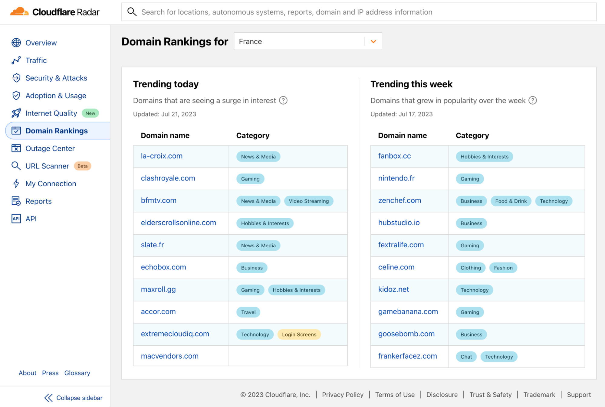
Today, we are improving our Domain Rankings page and adding Trending Domains lists. The new data shows which domains are currently experiencing an increase in popularity. Hence, while with the top popular domains we aim to show domains of broad appeal and of interest to many Internet users, with the trending domains we want to show domains that are generating a surge in interest.
How we generate the Trending Domains
When we started looking at the best way to generate a list of trending domains, we needed to answer the following questions:
What type of popularity changes do we want to capture?
What should we use as a baseline to calculate the change?
And how do we quantify it?
We soon realized that we needed two lists. One reflecting sudden increased interest related to a particular event or a topic, showing spikes in popularity in domains that jump in the ranking from one day to the next, and another one reflecting steady growth in popularity, showing domains that are increasing their user base over a longer period.
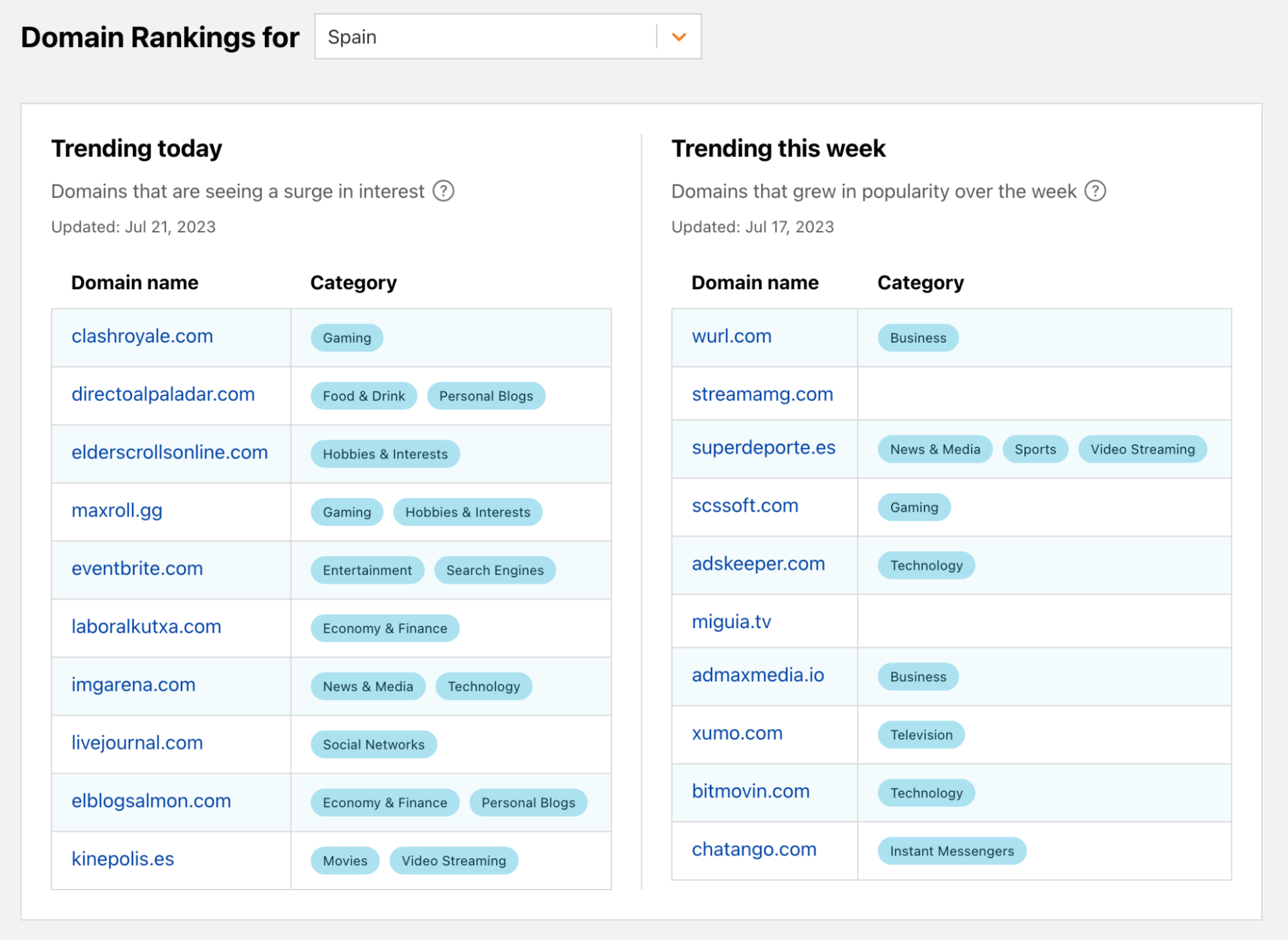
For this reason, we are launching both the Trending Today and Trending This Week top 10 lists to capture the two different types of popularity increase.
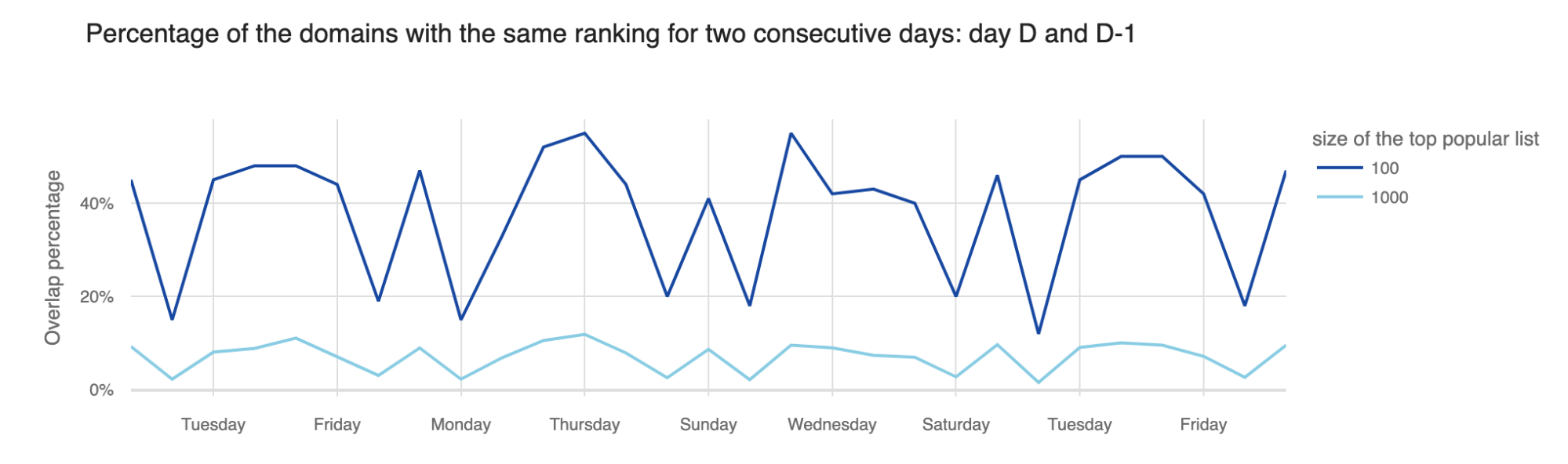
To select the baseline for calculating the increase in popularity, we analyzed the volatility of the Radar Domain Ranking list for different top list sizes. The advantage of starting with the Radar Ranking lists is that they already incorporate a good popularity metric that quantifies the estimated relative size of the user population that accesses a domain over some period of time. You can read more about how we define popularity in our “Goodbye, Alexa. Hello, Cloudflare Radar Domain Rankings” blog.
As expected, smaller list sizes were more stable, meaning the percentage of domains in the top 100 that changed the ranking from one day to the next was much lower than the percentage of domains that changed in the top 10,000. Hence, to have a dynamic daily list of trending domains, we had to look beyond the top 100 most popular domains.
However, we did not want to go all the way to the long tail of the list, as we already know that the ranks there are based on “significantly smaller and hence less reliable numbers” (see the paper "A Long Way to the Top: Significance, Structure, and Stability of Internet Top Lists"). Hence, we selected an appropriate list size for each location, based on the distribution of the number of DNS queries per domain. For example, for the Worldwide trending list we analyzed the top 20,000 most popular domains, for Brazil we looked at the top 10,000, Angola 5,000 and for the Faroe Islands top 500.
Trending Today
We then evaluated how much the domains change rank from one day to the next.
We saw that on average, the biggest changes in the top lists, from one day to the next, happen from Fridays to Saturdays and from Sundays to Mondays, and hence on Saturdays and Mondays the lists have the least overlap with the lists of the previous day. We also compared the rank changes from one day to the next corresponding weekday, say from one Monday to the next and saw that on average, rankings on Mondays typically have more overlap with the rankings of the previous Mondays, than with the rankings of Sunday. From this we decided that in order to capture which domains are trending due to the weekend effect, we needed to compare the domain's daily rank to the rank of the previous day(s), and not of the corresponding weekday.
However, we also did not want to show as trending those domains that highly oscillate in the rankings, jumping up and down from one day to the next, showing up as trending every few days. Hence, we could not simply compare the daily rank with the rank from the day before. Instead, as a compromise between capturing the most recent trends, including the weekend trends, but still filtering out the domains whose ranking oscillates over a short period of time, we decided to compare the domain's daily rank with its best rank of the previous four days.
Then, to calculate the increase in popularity, we simply calculate the percentage change in the current rank compared to the best rank of the previous four days.
Trending This Week
For calculating the domains steadily growing over the week, we used a slightly different approach.
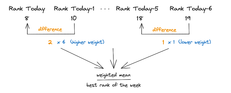
We want to highlight domains that keep improving their rank day by day and especially those that have been really trending in the most recent days. Therefore, we decided not to directly compare the current rank with the best rank during the previous week. Instead, we looked at the weighted average per day rank improvement and compared it with the best rank of the previous six days, with more recent days being given more weight.
Example trending domains
What do these lists look like at the end? We compiled the lists for the eventful days of June 21 to 24.
On June 22, nba.com was trending in 28 locations, shown in the table below, the United States, as expected, but also Austria, Australia and Japan, to name a few, reflecting the interest in the events of NBA Draft 2023.
Trending Today data from Friday, June 23, 2023:
Location
Trending rank
Domain
Albania
5
nba.com
Argentina
9
nba.com
Australia
1
nba.com
Austria
9
nba.com
Belgium
5
nba.com
Canada
5
nba.com
Chile
6
nba.com
Colombia
3
nba.com
Dominican Republic
5
nba.com
Greece
2
nba.com
Honduras
6
nba.com
Hong Kong
1
nba.com
India
7
nba.com
Indonesia
4
nba.com
Ireland
3
nba.com
Japan
9
nba.com
Mexico
2
nba.com
New Zealand
1
nba.com
Norway
1
nba.com
Philippines
1
nba.com
Poland
9
nba.com
Serbia
2
nba.com
South Korea
3
nba.com
Taiwan
1
nba.com
Thailand
1
nba.com
Ukraine
1
nba.com
United States
6
nba.com
Venezuela
4
nba.com
Two domains trending in multiple locations on Saturday, June 24, were: rt.com, a Russian news site in English, and liveuamap.com, a site with interactive map of Ukraine. These are probably the effects of the events related to the Wagner group on June 23 and 24. Related to the same events, domain jetphotos.com was trending on the same day in Russia, Norway and Albania.
Trending Today data from Saturday, June 24, 2023:
Location
Trending rank
Domain
Armenia
4
rt.com
Australia
5
rt.com
Belgium
2
rt.com
Bulgaria
9
rt.com
Canada
6
rt.com
Denmark
6
rt.com
Greece
6
rt.com
Italy
2
rt.com
Kazakhstan
8
rt.com
Lebanon
4
rt.com
Netherlands
8
rt.com
Papua New Guinea
9
rt.com
Singapore
2
rt.com
Spain
6
rt.com
Turkey
4
rt.com
United Kingdom
5
rt.com
United States
3
rt.com
Uzbekistan
2
rt.com
Other domains trending in various locations on Friday and Saturday were different Gaming and Video Streaming domains such as roblox.com, twitch.tv and callofduty.com, showing an increased interest in gaming activities as the weekend approaches.
Yet another interesting effect of the weekend was the presence of five weather forecast sites on the top 10 trending sites on Friday, in Croatia, showing preoccupation with the summer weekend plans.
Trending Today in Croatia (data from Friday, June 23, 2023)
Trending rank
Domain
Category
1
lightningmaps.org
Weather; Education
2
freemeteo.com.hr
Weather
3
Vrijeme.hr (Croatian Meteorological and Hydrological Service)
Politics, Advocacy, and Government-Related
4
arso.gov.si
5
rain-alarm.com
Weather; News & Media
6
sorbs.net
Information Security
7
neverin.hr
Information Technology
8
meteo.hr (Croatian Meteorological and Hydrological Service)
Business
9
gamespot.com
Gaming; Video Streaming
10
grad.hr
Business
These were all examples of daily trending domains, but what domains have steadily grown in popularity that week?
In multiple countries we had travel sites trending that week, sites such as booking.com, rentcars.com and amadeus.com, as many people were making their summer vacation plans. Weather forecast, specifically windy.com domain, was also trending the whole week in locations such as the Dominican Republic, Saint Lucia and Reunion, which was not surprising as the hurricane season began.
Trending This Week (Week June 17 -23, 2023)
Dominican Republic
Reunion
Saint Lucia
cecomsa.com
atera.com
adition.com
blur.io
sharethis.com
windy.com
pxfuel.com
windy.com
bbc.co.uk
windy.com
baidu.com
ampproject.org
mihoyo.com
inmobi.com
aniview.com
Final words
Both Trending Today and Trending This Week top 10 lists are now available on Radar starting today and on Radar API. Feel free to explore them and see what is trending on the Internet.
Visit Cloudflare Radar for additional insights around (Internet disruptions, routing issues, Internet traffic trends, attacks, Internet quality, etc.). Follow us on social media at @CloudflareRadar (Twitter), cloudflare.social/@radar (Mastodon), and radar.cloudflare.com (Bluesky), or contact us via e-mail.
Popular domains are domains of broad appeal based on how people use the Internet. Trending domains are domains that are generating a surge in interest.
To provide the best experiences, we use technologies like cookies to store and/or access device information. Consenting to these technologies will allow us to process data such as browsing behavior or unique IDs on this site. Not consenting or withdrawing consent, may adversely affect certain features and functions.
Functional
Always active
The technical storage or access is strictly necessary for the legitimate purpose of enabling the use of a specific service explicitly requested by the subscriber or user, or for the sole purpose of carrying out the transmission of a communication over an electronic communications network.
Preferences
The technical storage or access is necessary for the legitimate purpose of storing preferences that are not requested by the subscriber or user.
Statistics
The technical storage or access that is used exclusively for statistical purposes.The technical storage or access that is used exclusively for anonymous statistical purposes. Without a subpoena, voluntary compliance on the part of your Internet Service Provider, or additional records from a third party, information stored or retrieved for this purpose alone cannot usually be used to identify you.
Marketing
The technical storage or access is required to create user profiles to send advertising, or to track the user on a website or across several websites for similar marketing purposes.