Post Syndicated from Austin Groeneveld original https://aws.amazon.com/blogs/big-data/optimize-traffic-costs-of-amazon-msk-consumers-on-amazon-eks-with-rack-awareness/
Are you incurring significant cross Availability Zone traffic costs when running an Apache Kafka client in containerized environments on Amazon Elastic Kubernetes Service (Amazon EKS) that consume data from Amazon Managed Streaming for Apache Kafka (Amazon MSK) topics?
If you’re not familiar with Apache Kafka’s rack awareness feature, we strongly recommend starting with the blog post on how to Reduce network traffic costs of your Amazon MSK consumers with rack awareness for an in-depth explanation of the feature and how Amazon MSK supports it.
Although the solution described in that post uses an Amazon Elastic Compute Cloud (Amazon EC2) instance deployed in a single Availability Zone to consume messages from an Amazon MSK topic, modern cloud-native architectures demand more dynamic and scalable approaches. Amazon EKS has emerged as a leading platform for deploying and managing distributed applications. The dynamic nature of Kubernetes introduces unique implementation challenges compared to static client deployments. In this post, we walk you through a solution for implementing rack awareness in consumer applications that are dynamically deployed across multiple Availability Zones using Amazon EKS.
Here’s a quick recap of some key Apache Kafka terminology from the referenced blog. An Apache Kafka client consumer will register to read against a topic. A topic is the logical data structure that Apache Kafka organizes data into. A topic is segmented into a single or many partitions. Partitions are the unit of parallelism in Apache Kafka. Amazon MSK provides high availability by replicating each partition of a topic across brokers in different Availability Zones. Because there are replicas of each partition that reside across the different brokers that make up your MSK cluster, Amazon MSK also tracks whether a replica partition is in sync with the most recent data for that partition. This means there is one partition that Amazon MSK recognizes as containing the most up-to-date data, and this is known as the leader partition. The collection of replicated partitions is called in-sync replicas. This list of in-sync replicas is used internally when the cluster needs to elect a new leader partition if the current leader were to become unavailable.
When consumer applications read from a topic, the Apache Kafka protocol facilitates a network exchange to determine which broker currently has the leader partition that the consumer needs to read from. This means that the consumer could be told to read from a broker in a different Availability Zone than itself, leading to cross-zone traffic charge in your AWS account. To help optimize this cost, Amazon MSK supports the rack awareness feature, using which clients can ask an Amazon MSK cluster to provide a replica partition to read from, within the same Availability Zone as the client, even if it isn’t the current leader partition. The cluster accomplishes this by checking for an in-sync replica on a broker within the same Availability Zone as the consumer.
The challenge with Kafka clients on Amazon EKS
In Amazon EKS, the underlying units of computes are EC2 instances that are abstracted as Kubernetes nodes. The nodes are organized into node groups for ease of management, scaling, and grouping of applications on certain EC2 instance types. As a best practice for resilience, the nodes in a node group are spread across multiple Availability Zones. Amazon EKS uses the underlying Amazon EC2 metadata about the Availability Zone that it’s located in, and it injects that information into the node’s metadata during node configuration. In particular, the Availability Zone (AZ ID) is injected into the node metadata.
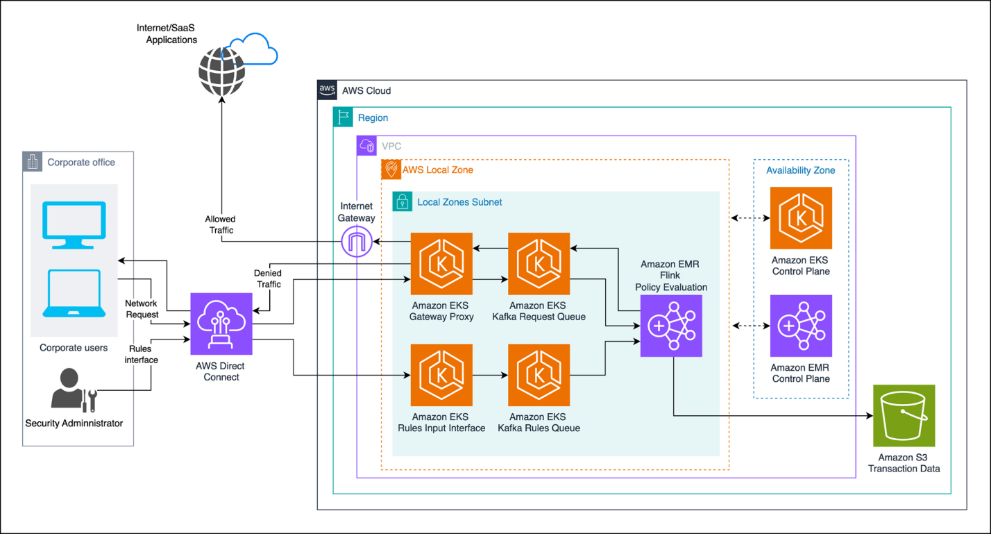
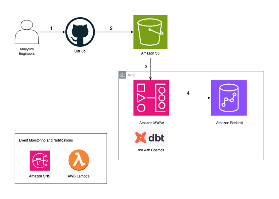
When an application is deployed in a Kubernetes Pod on Amazon EKS, it goes through a process of binding to a node that meets the pod’s requirements. As shown in the following diagram, when you deploy client applications on Amazon EKS, the pod for the application can be bound to a node with available capacity in any Availability Zone. Also, the pod doesn’t automatically inherit the Availability Zone information from the node that it’s bound to, a piece of information necessary for rack awareness. The following architecture diagram illustrates Kafka consumers running on Amazon EKS without rack awareness.

To set the client configuration for rack awareness, the pod needs to know what Availability Zone it’s located in, dynamically, as it is bound to a node. During its lifecycle, the same pod can be evicted from the node it was bound to previously and moved to a node in a different Availability Zone, if the matching criteria permit that. Making the pod aware of its Availability Zone dynamically sets the rack awareness parameter client.rack during the initialization of the application container that is encapsulated in the pod.
After rack awareness is enabled on the MSK cluster, what happens if the broker in the same Availability Zone as the client (hosted on Amazon EKS or elsewhere) becomes unavailable? The Apache Kafka protocol is designed to support a distributed data storage system. Assuming customers follow the best practice of implementing a replication factor > 1, Apache Kafka can dynamically reroute the consumer client to the next available in-sync replica on a different broker. This resilience remains consistent even after implementing nearest replica fetching, or rack awareness. Enabling rack awareness optimizes the networking exchange to prefer a partition within the same Availability Zone, but it doesn’t compromise the consumer’s ability to operate if the nearest replica is unavailable.
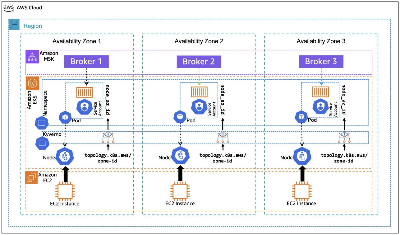
In this post, we walk you through an example of how to use the Kubernetes metadata label, topology.k8s.aws/zone-id, assigned to each node by Amazon EKS, and use an open source policy engine, Kyverno, to deploy a policy that mutates the pods that are in the binding state to dynamically inject the node’s AZ ID into the pod’s metadata as an annotation, as depicted in the following diagram. This annotation, in turn, is used by the container to create an environment variable that is assigned the pod’s annotated AZ ID information. The environment variable is then used in the container postStart lifecycle hook to generate the Kafka client configuration file with rack awareness setting. The following architecture diagram illustrates Kafka consumers running on Amazon EKS with rack awareness.

Solution Walkthrough
Prerequisites
For this walkthrough, we use AWS CloudShell to run the scripts that are provided inline as you progress. For a smooth experience, before getting started, make sure to have kubectl and eksctl installed and configured in the AWS CloudShell environment, following the installation instructions for Linux (amd64). Helm is also required to be install on AWS CloudShell, using the instructions for Linux.
Also, check if the envsubst tool is installed in your CloudShell environment by invoking:
If the tool isn’t installed, you can install it using the command:
sudo dnf -y install gettext-devel
We also assume you already have an MSK cluster deployed in an Amazon Virtual Private Cloud (VPC) in three Availability Zones with the name MSK-AZ-Aware. In this walkthrough, we use AWS Identity and Access Management (IAM) authentication for client access control to the MSK cluster. If you’re using a cluster in your account with a different name, replace the instances of MSK-AZ-Aware in the instructions.
We follow the same MSK cluster configuration mentioned in the Rack Awareness blog mentioned previously, with some modifications. (Ensure you’ve set replica.selector.class = org.apache.kafka.common.replica.RackAwareReplicaSelector for the reasons discussed there). In our configuration, we add one line: num.partitions = 6. Although not mandatory, this ensures that topics that are automatically created will have multiple partitions to support clearer demonstrations in subsequent sections.
Finally, we use the Amazon MSK Data Generator with the following configuration:
{
"name": "msk-data-generator",
    "config": {
    "connector.class": "com.amazonaws.mskdatagen.GeneratorSourceConnector",
    "genkp.MSK-AZ-Aware-Topic.with": "#{Internet.uuid}",
    "genv.MSK-AZ-Aware-Topic.product_id.with": "#{number.number_between '101','200'}",
    "genv.MSK-AZ-Aware-Topic.quantity.with": "#{number.number_between '1','5'}",
    "genv.MSK-AZ-Aware-Topic.customer_id.with": "#{number.number_between '1','5000'}"
    }
}
Running the MSK Data Generator with this configuration will automatically create a six-partition topic named MSK-AZ-Aware-Topic on our cluster for us, and it will push data to that topic. To follow along with the walkthrough, we recommend and assume that you deploy the MSK Data Generator to create the topic and populate it with simulated data.
Create the EKS cluster
The first step is to install an EKS cluster in the same Amazon VPC subnets as the MSK cluster. You can modify the name of the MSK cluster by changing that environment variable MSK_CLUSTER_NAME if your cluster is created with a different name than suggested. You can also change the Amazon EKS cluster name by changing EKS_CLUSTER_NAME.
The environment variables that we define here are used throughout the walkthrough.
The last step is to update the kubeconfig with an entry for the EKS cluster:
AWS_ACCOUNT=$(aws sts get-caller-identity --output text --query Account)
export AWS_ACCOUNT
export AWS_REGION=${AWS_DEFAULT_REGION}
export MSK_CLUSTER_NAME=MSK-AZ-Aware
export EKS_CLUSTER_NAME=EKS-AZ-Aware
export EKS_CLUSTER_SIZE=3
export K8S_VERSION=1.32
export POD_ID_VERSION=1.3.5

MSK_BROKER_SG=$(aws kafka list-clusters \
  --query  'ClusterInfoList[?ClusterName==`'${MSK_CLUSTER_NAME}'`].BrokerNodeGroupInfo.SecurityGroups'  \
  --output text | xargs)
export MSK_BROKER_SG

MSK_BROKER_CLIENT_SUBNETS=$(aws kafka list-clusters \
  --query  'ClusterInfoList[?ClusterName==`'${MSK_CLUSTER_NAME}'`].BrokerNodeGroupInfo.ClientSubnets'  \
  --output text | xargs)
export MSK_BROKER_CLIENT_SUBNETS

VPC_ID=$(aws ec2 describe-subnets \
  --subnet-ids "$(echo "${MSK_BROKER_CLIENT_SUBNETS}" | cut -d' ' -f1)" \
  --query 'Subnets[0].VpcId' \
  --output text)
export VPC_ID

EKS_SUBNETS=$(echo ${MSK_BROKER_CLIENT_SUBNETS} | sed 's/ \+/,/g')
export EKS_SUBNETS

# Create a minimal config file for encrypted node volumes
cat > eks-config.yaml << EOF
apiVersion: eksctl.io/v1alpha5
kind: ClusterConfig
metadata:
  name: ${EKS_CLUSTER_NAME}
  region: ${AWS_REGION}
  version: "${K8S_VERSION}"
vpc:
  id: "${VPC_ID}"
  subnets:
    public:
$(for subnet in ${MSK_BROKER_CLIENT_SUBNETS}; do
  AZ=$(aws ec2 describe-subnets --subnet-ids "$subnet" --query 'Subnets[0].AvailabilityZone' --output text)
  echo "      $AZ: { id: $subnet }"
done)
nodeGroups:
  - name: ng1
    instanceType: m5.xlarge
    desiredCapacity: ${EKS_CLUSTER_SIZE}
    minSize: ${EKS_CLUSTER_SIZE}
    maxSize: ${EKS_CLUSTER_SIZE}
    securityGroups:
      attachIDs: ["${MSK_BROKER_SG}"]
    volumeSize: 100
    volumeType: gp3
    volumeEncrypted: true
EOF

eksctl create cluster -f eks-config.yaml

aws eks update-kubeconfig \
  --region "${AWS_REGION}" \
  --name ${EKS_CLUSTER_NAME}
Next, you need to create an IAM policy, MSK-AZ-Aware-Policy, to allow access from the Amazon EKS pods to the MSK cluster. Note here that we’re using MSK-AZ-Aware as the cluster name.
Create a file, msk-az-aware-policy.json, with the IAM policy template:
cat > msk-az-aware-policy.json << EOF
{
    "Version": "2012-10-17",
    "Statement": [
        {
            "Effect": "Allow",
            "Action": [
                "kafka-cluster:Connect",
                "kafka-cluster:AlterCluster",
                "kafka-cluster:DescribeCluster",
                "kafka-cluster:DescribeClusterDynamicConfiguration",
                "kafka-cluster:AlterClusterDynamicConfiguration"
            ],
            "Resource": [
                "arn:aws:kafka:${AWS_REGION}:${AWS_ACCOUNT}:cluster/${MSK_CLUSTER_NAME}/*"
            ]
        },
        {
            "Effect": "Allow",
            "Action": [
                "kafka-cluster:*Topic*",
                "kafka-cluster:WriteData",
                "kafka-cluster:ReadData"
            ],
            "Resource": [
                "arn:aws:kafka:${AWS_REGION}:${AWS_ACCOUNT}:topic/${MSK_CLUSTER_NAME}/*"
            ]
        },
        {
            "Effect": "Allow",
            "Action": [
                "kafka-cluster:AlterGroup",
                "kafka-cluster:DescribeGroup"
            ],
            "Resource": [
                "arn:aws:kafka:${AWS_REGION}:${AWS_ACCOUNT}:group/${MSK_CLUSTER_NAME}/*"
            ]
        }
    ]
}
EOF
To create the IAM policy, use the following command. It first replaces the placeholders in the policy file with values from relevant environment variables, and then creates the IAM policy:
envsubst < msk-az-aware-policy.json | \
xargs -0 -I {} aws iam create-policy \
            --policy-name MSK-AZ-Aware-Policy \
            --policy-document {}
Configure EKS Pod Identity
Amazon EKS Pod Identity offers a simplified experience for obtaining IAM permissions for pods on Amazon EKS. This requires installing an add-on Amazon EKS Pod Identity Agent to the EKS cluster:
eksctl create addon \
  --cluster ${EKS_CLUSTER_NAME} \
  --name eks-pod-identity-agent \
  --version ${POD_ID_VERSION}
Confirm that the add-on has been installed and its status is ACTIVE and that the status of all the pods associated with the add-on is Running.
eksctl get addon \
  --cluster ${EKS_CLUSTER_NAME} \
  --region "${AWS_REGION}" \
  --name eks-pod-identity-agent -o json

kubectl get pods \
  -n kube-system \
  -l app.kubernetes.io/instance=eks-pod-identity-agent
After you’ve installed the add-on, you need to create a pod identity association between a Kubernetes service account and the IAM policy created earlier:
eksctl create podidentityassociation \
  --namespace kafka-ns \
  --service-account-name kafka-sa \
  --role-name EKS-AZ-Aware-Role \
  --permission-policy-arns arn:aws:iam::"${AWS_ACCOUNT}":policy/MSK-AZ-Aware-Policy \
  --cluster ${EKS_CLUSTER_NAME} \
  --region "${AWS_REGION}"
Install Kyverno
Kyverno is an open source policy engine for Kubernetes that allows for validation, mutation, and generation of Kubernetes resources using policies written in YAML, thus simplifying the enforcement of security and compliance requirements. You need to install Kyverno to dynamically inject metadata into the Amazon EKS pods as they enter the binding state to inform them of Availability Zone ID.
In AWS CloudShell, create a file named kyverno-values.yaml. This file defines the Kubernetes RBAC permissions for Kyverno’s Admission Controller to read Amazon EKS node metadata because the default Kyverno (v. 1.13 onwards) settings don’t allow this:
cat > kyverno-values.yaml << EOF
admissionController:
  rbac:
    clusterRole:
      extraResources:
        - apiGroups:
            - ""
          resources:
            - "nodes"
          verbs:
            - get
            - list
            - watch
EOF
After this file is created, you can install Kyverno using helm and providing the values file created in the previous step:
helm repo add kyverno https://kyverno.github.io/kyverno/
helm repo update

helm install kyverno kyverno/kyverno \
  -n kyverno \
  --create-namespace \
  --version 3.3.7 \
  -f kyverno-values.yaml
Starting with Kyverno v 1.13, the Admission Controller is configured to ignore the AdmissionReview requests for pods in binding state. This needs to be changed by editing the Kyverno ConfigMap:
kubectl -n kyverno edit configmap kyverno
The kubectl edit command uses the default editor configured in your environment (in our case Linux VIM).
This will open the ConfigMap in a text editor.
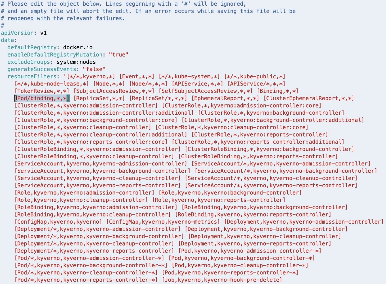
As highlighted in the following screenshot, [Pod/binding,*,*] should be removed from the resourceFilters field for the Kyverno Admission Controller to process AdmissionReview requests for pods in binding state.

If Linux VIM is your default editor, you can delete the entry using VIM command 18x, meaning delete (or cut) 18 characters from the current cursor position. Save the modified configuration using the VIM command :wq, meaning write (or save) the file and quit.
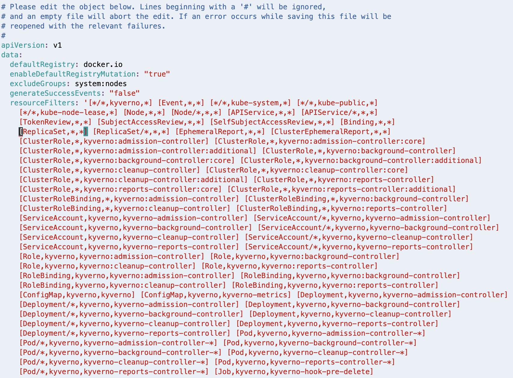
After deleting, the resourceFilters field should look similar to the following screenshot.

If you have a different editor configured in your environment, follow the appropriate steps to achieve a similar outcome.
Configure Kyverno policy
You need to configure the policy that will make the pods rack aware. This policy is adapted from the suggested approach in the Kyverno blog post, Assigning Node Metadata to Pods. Create a new file with the name kyverno-inject-node-az-id.yaml:
cat > kyverno-inject-node-az-id.yaml  << EOF
apiVersion: kyverno.io/v2beta1
kind: ClusterPolicy
metadata:
  name: inject-node-az-id
spec:
  background: false
  rules:
    - name: inject-node-az-id
      match:
        any:
        - resources:
            kinds:
            - Pod/binding
      context:
      - name: node
        variable:
          jmesPath: request.object.target.name
          default: ''
      - name: node_az_id
        apiCall:
          urlPath: "/api/v1/nodes/{{node}}"
          jmesPath: "metadata.labels.\"topology.k8s.aws/zone-id\" || 'empty'"
      mutate:
        patchStrategicMerge:
          metadata:
            annotations:
              node_az_id: "{{ node_az_id }}"
EOF
It instructs Kyverno to watch for pods in binding state. After Kyverno receives the AdmissionReview request for a pod, it sets the variable node to the name of the node to which the pod is being bound. It also sets another variable node_az_id to the Availability Zone ID by calling the Kubernetes API /api/v1/nodes/node to get the node metadata label topology.k8s.aws/zone-id. Finally, it defines a mutate rule to inject the obtained AZ ID into the pod’s metadata as an annotation node_az_id.
After you’ve created the file, apply the policy using the following command:
kubectl apply -f kyverno-inject-node-az-id.yaml
Deploy a pod without rack awareness
Now let’s visualize the problem statement. To do this, connect to one of the EKS pods and check how it interacts with the MSK cluster when you run a Kafka consumer from the pod.
First, get the bootstrap string of the MSK cluster. Look up the Amazon Resource Names (ARNs) of the MSK cluster:
MSK_CLUSTER_ARN=$(
    aws kafka list-clusters \
      --query 'ClusterInfoList[?ClusterName==`'${MSK_CLUSTER_NAME}'`].ClusterArn' \
      --output text)
export MSK_CLUSTER_ARN
Using the cluster ARN, you can get the bootstrap string with the following command:
BOOTSTRAP_SERVER_LIST=$(
    aws kafka get-bootstrap-brokers \
        --cluster-arn "${MSK_CLUSTER_ARN}" \
        --query 'BootstrapBrokerStringSaslIam' \
        --output text)
export BOOTSTRAP_SERVER_LIST
Create a new file named kafka-no-az.yaml:
cat > kafka-no-az.yaml << EOF
apiVersion: v1
kind: Namespace
metadata:
 name: kafka-ns
---
apiVersion: v1
kind: ServiceAccount
metadata:
 name: kafka-sa
 namespace: kafka-ns
automountServiceAccountToken: false
---
apiVersion: apps/v1
kind: Deployment
metadata:
  name: kafka-no-az
  namespace: kafka-ns
  labels:
    app: kafka-no-az
  annotations:
    node_az_id: ''
spec:
  replicas: 3
  selector:
    matchLabels:
      app: kafka-no-az
  template:
    metadata:
      labels:
        app: kafka-no-az
    spec:
      serviceAccountName: kafka-sa
      containers:
      - image: bitnami/kafka:3.8.0
        name: kafka-no-az
        command: ["/bin/sh", "-ec", "while :; do echo '.'; sleep 5 ; done"]
        env:
        - name: BootstrapServerString
          value: ${BOOTSTRAP_SERVER_LIST}
        - name: MSK_TOPIC
          value: "MSK-AZ-Aware-Topic"
        - name: KAFKA_HOME
          value: /opt/bitnami/kafka
        - name: KAFKA_BIN
          value: /opt/bitnami/kafka/bin
        - name: KAFKA_CONFIG
          value: /opt/bitnami/kafka/config
        - name: KAFKA_LIBS
          value: /opt/bitnami/kafka/libs
        - name: KAFKA_LOG4J_OPTS
          value: "-Dlog4j.configuration=file:/opt/bitnami/kafka/config/log4j.properties"
        lifecycle:
          postStart:
            exec:
              command:
              - "sh"
              - "-c"
              - |
                export KAFKA_HOME=/opt/bitnami/kafka
                export KAFKA_BIN=\${KAFKA_HOME}/bin
                export KAFKA_CONFIG=\${KAFKA_HOME}/config
                cat > \${KAFKA_CONFIG}/client.properties << EOF1
                security.protocol=SASL_SSL
                sasl.mechanism=AWS_MSK_IAM
                sasl.jaas.config=software.amazon.msk.auth.iam.IAMLoginModule required;
                sasl.client.callback.handler.class=software.amazon.msk.auth.iam.IAMClientCallbackHandler
                EOF1

                cat >> \${KAFKA_CONFIG}/log4j.properties << EOF2
                #
                # Enable logging of Kafka Client to stderr
                #
                log4j.rootLogger=WARN, stderr
                log4j.logger.org.apache.kafka.clients.consumer.internals.AbstractFetch=DEBUG
                log4j.appender.stderr=org.apache.log4j.ConsoleAppender
                log4j.appender.stderr.layout=org.apache.log4j.PatternLayout
                log4j.appender.stderr.layout.ConversionPattern=[%d] %p %m (%c)%n
                log4j.appender.stderr.Target=System.err
                EOF2
                cd \${KAFKA_HOME}/libs
                /usr/bin/curl -sS -L https://github.com/aws/aws-msk-iam-auth/releases/download/v2.2.0/aws-msk-iam-auth-2.2.0-all.jar --output \${KAFKA_LIBS}/aws-msk-iam-auth-2.2.0-all.jar
EOF
This pod manifest doesn’t make use of the Availability Zone ID injected into the metadata annotation and hence doesn’t add client.rack to the client.properties configuration.
Deploy the pods using the following command:
kubectl apply -f kafka-no-az.yaml
Run the following command to confirm that the pods have been deployed and are in the Running state:
kubectl -n kafka-ns get pods
Select a pod id from the output of the previous command, and connect to it using:
kubectl -n kafka-ns exec -it POD_ID -- sh
Run the Kafka consumer:
"${KAFKA_BIN}"/kafka-console-consumer.sh \
  --bootstrap-server  "${BootstrapServerString}" \
  --consumer.config  "${KAFKA_CONFIG}"/client.properties \
  --topic "${MSK_TOPIC}" \
  --from-beginning /tmp/non-rack-aware-consumer.log 2>&1 &
This command will dump all the resulting logs into the file, non-rack-aware-consumer.log. There’s a lot of information in those logs, and we encourage you to open them and take a deeper look. Next, examine the EKS pod in action. To do this, run the following command to tail the file to view fetch request results to the MSK cluster. You’ll notice a handful of meaningful logs to review as the consumer access various partitions of the Kafka topic:
grep -E "DEBUG.*Added read_uncommitted fetch request for partition MSK-AZ-Aware-Topic-[0-9]+" /tmp/rack-aware-consumer.log | tail -5
Observe your log output, which should look similar to the following:
[2025-03-12 23:59:05,308] DEBUG [Consumer clientId=console-consumer, groupId=console-consumer-24102] Added read_uncommitted fetch request for partition MSK-AZ-Aware-Topic-3 at position FetchPosition{offset=100, offsetEpoch=Optional[0], currentLeader=LeaderAndEpoch{leader=Optional[b-2.mskazaware.hxrzlh.c6.kafka.us-east-1.amazonaws.com:9098 (id: 2 rack: use1-az6)], epoch=0}} to node b-2.mskazaware.hxrzlh.c6.kafka.us-east-1.amazonaws.com:9098 (id: 2 rack: use1-az6) (org.apache.kafka.clients.consumer.internals.AbstractFetch)
[2025-03-12 23:59:05,308] DEBUG [Consumer clientId=console-consumer, groupId=console-consumer-24102] Added read_uncommitted fetch request for partition MSK-AZ-Aware-Topic-0 at position FetchPosition{offset=83, offsetEpoch=Optional[0], currentLeader=LeaderAndEpoch{leader=Optional[b-2.mskazaware.hxrzlh.c6.kafka.us-east-1.amazonaws.com:9098 (id: 2 rack: use1-az6)], epoch=0}} to node b-2.mskazaware.hxrzlh.c6.kafka.us-east-1.amazonaws.com:9098 (id: 2 rack: use1-az6) (org.apache.kafka.clients.consumer.internals.AbstractFetch)
[2025-03-12 23:59:05,542] DEBUG [Consumer clientId=console-consumer, groupId=console-consumer-24102] Added read_uncommitted fetch request for partition MSK-AZ-Aware-Topic-5 at position FetchPosition{offset=100, offsetEpoch=Optional[0], currentLeader=LeaderAndEpoch{leader=Optional[b-1.mskazaware.hxrzlh.c6.kafka.us-east-1.amazonaws.com:9098 (id: 1 rack: use1-az4)], epoch=0}} to node b-1.mskazaware.hxrzlh.c6.kafka.us-east-1.amazonaws.com:9098 (id: 1 rack: use1-az4) (org.apache.kafka.clients.consumer.internals.AbstractFetch)
[2025-03-12 23:59:05,542] DEBUG [Consumer clientId=console-consumer, groupId=console-consumer-24102] Added read_uncommitted fetch request for partition MSK-AZ-Aware-Topic-2 at position FetchPosition{offset=107, offsetEpoch=Optional[0], currentLeader=LeaderAndEpoch{leader=Optional[b-1.mskazaware.hxrzlh.c6.kafka.us-east-1.amazonaws.com:9098 (id: 1 rack: use1-az4)], epoch=0}} to node b-1.mskazaware.hxrzlh.c6.kafka.us-east-1.amazonaws.com:9098 (id: 1 rack: use1-az4) (org.apache.kafka.clients.consumer.internals.AbstractFetch)
[2025-03-12 23:59:05,720] DEBUG [Consumer clientId=console-consumer, groupId=console-consumer-24102] Added read_uncommitted fetch request for partition MSK-AZ-Aware-Topic-4 at position FetchPosition{offset=84, offsetEpoch=Optional[0], currentLeader=LeaderAndEpoch{leader=Optional[b-3.mskazaware.hxrzlh.c6.kafka.us-east-1.amazonaws.com:9098 (id: 3 rack: use1-az2)], epoch=0}} to node b-3.mskazaware.hxrzlh.c6.kafka.us-east-1.amazonaws.com:9098 (id: 3 rack: use1-az2) (org.apache.kafka.clients.consumer.internals.AbstractFetch)
[2025-03-12 23:59:05,720] DEBUG [Consumer clientId=console-consumer, groupId=console-consumer-24102] Added read_uncommitted fetch request for partition MSK-AZ-Aware-Topic-1 at position FetchPosition{offset=85, offsetEpoch=Optional[0], currentLeader=LeaderAndEpoch{leader=Optional[b-3.mskazaware.hxrzlh.c6.kafka.us-east-1.amazonaws.com:9098 (id: 3 rack: use1-az2)], epoch=0}} to node b-3.mskazaware.hxrzlh.c6.kafka.us-east-1.amazonaws.com:9098 (id: 3 rack: use1-az2) (org.apache.kafka.clients.consumer.internals.AbstractFetch)
[2025-03-12 23:59:05,811] DEBUG [Consumer clientId=console-consumer, groupId=console-consumer-24102] Added read_uncommitted fetch request for partition MSK-AZ-Aware-Topic-3 at position FetchPosition{offset=100, offsetEpoch=Optional[0], currentLeader=LeaderAndEpoch{leader=Optional[b-2.mskazaware.hxrzlh.c6.kafka.us-east-1.amazonaws.com:9098 (id: 2 rack: use1-az6)], epoch=0}} to node b-2.mskazaware.hxrzlh.c6.kafka.us-east-1.amazonaws.com:9098 (id: 2 rack: use1-az6) (org.apache.kafka.clients.consumer.internals.AbstractFetch)
[2025-03-12 23:59:05,811] DEBUG [Consumer clientId=console-consumer, groupId=console-consumer-24102] Added read_uncommitted fetch request for partition MSK-AZ-Aware-Topic-0 at position FetchPosition{offset=83, offsetEpoch=Optional[0], currentLeader=LeaderAndEpoch{leader=Optional[b-2.mskazaware.hxrzlh.c6.kafka.us-east-1.amazonaws.com:9098 (id: 2 rack: use1-az6)], epoch=0}} to node b-2.mskazaware.hxrzlh.c6.kafka.us-east-1.amazonaws.com:9098 (id: 2 rack: use1-az6) (org.apache.kafka.clients.consumer.internals.AbstractFetch)
You’ve now connected to a specific pod in the EKS cluster and run a Kafka consumer to read from the MSK topic without rack awareness. Remember that this pod is running within a single Availability Zone.
Reviewing the log output, you find rack: values as use1-az2, use1-az4, and use1-az6 as the pod makes calls to different partitions of the topic. These rack values represent the Availability Zone IDs that our brokers are running within. This means that our EKS pod is creating networking connections to brokers across three different Availability Zones, which would be accruing networking charges in our account.
Also notice that you have no way to check which node, and therefore Availability Zone, this EKS pod is running in. You can observe in the logs that it’s calling to MSK brokers in different Availability Zones, but there is no way to know which broker is in the same Availability Zone as the EKS pod you’ve connected to. Delete the deployment when you’re done:
kubectl -n kafka-ns delete -f kafka-no-az.yaml
Deploy a pod with rack awareness
Now that you have experienced the consumer behavior without rack awareness, you need to inject the Availability Zone ID to make your pods rack-aware.
Create a new file named kafka-az-aware.yaml:
cat > kafka-az-aware.yaml << EOF
apiVersion: v1
kind: Namespace
metadata:
 name: kafka-ns
---
apiVersion: v1
kind: ServiceAccount
metadata:
 name: kafka-sa
 namespace: kafka-ns
automountServiceAccountToken: false
---
apiVersion: apps/v1
kind: Deployment
metadata:
  name: kafka-az-aware
  namespace: kafka-ns
  labels:
    app: kafka-az-aware
  annotations:
    node_az_id: ''
spec:
  replicas: 3
  selector:
    matchLabels:
      app: kafka-az-aware
  template:
    metadata:
      labels:
        app: kafka-az-aware
    spec:
      serviceAccountName: kafka-sa
      containers:
      - image: bitnami/kafka:3.8.0
        name: kafka-az-aware
        command: ["/bin/sh", "-ec", "while :; do echo '.'; sleep 5 ; done"]
        env:
        - name: BootstrapServerString
          value: ${BOOTSTRAP_SERVER_LIST}
        - name: MSK_TOPIC
          value: "MSK-AZ-Aware-Topic"
        - name: KAFKA_HOME
          value: /opt/bitnami/kafka
        - name: KAFKA_BIN
          value: /opt/bitnami/kafka/bin
        - name: KAFKA_CONFIG
          value: /opt/bitnami/kafka/config
        - name: KAFKA_LIBS
          value: /opt/bitnami/kafka/libs
        - name: KAFKA_LOG4J_OPTS
          value: "-Dlog4j.configuration=file:/opt/bitnami/kafka/config/log4j.properties"
        - name: NODE_AZ_ID
          valueFrom:
            fieldRef:
              fieldPath: metadata.annotations['node_az_id']
        lifecycle:
          postStart:
            exec:
              command:
              - "sh"
              - "-c"
              - |
                export KAFKA_HOME=/opt/bitnami/kafka
                export KAFKA_BIN=\${KAFKA_HOME}/bin
                export KAFKA_CONFIG=\${KAFKA_HOME}/config
                cat > \${KAFKA_CONFIG}/client.properties << EOF1
                security.protocol=SASL_SSL
                sasl.mechanism=AWS_MSK_IAM
                sasl.jaas.config=software.amazon.msk.auth.iam.IAMLoginModule required;
                sasl.client.callback.handler.class=software.amazon.msk.auth.iam.IAMClientCallbackHandler
                EOF1
                if [ \$NODE_AZ_ID ]
                then
                  echo "client.rack=\$NODE_AZ_ID" >> \${KAFKA_CONFIG}/client.properties
                fi

                cat >> \${KAFKA_CONFIG}/log4j.properties << EOF2
                #
                # Enable logging of Kafka Client to stderr
                #
                log4j.rootLogger=WARN, stderr
                log4j.logger.org.apache.kafka.clients.consumer.internals.AbstractFetch=DEBUG
                log4j.appender.stderr=org.apache.log4j.ConsoleAppender
                log4j.appender.stderr.layout=org.apache.log4j.PatternLayout
                log4j.appender.stderr.layout.ConversionPattern=[%d] %p %m (%c)%n
                log4j.appender.stderr.Target=System.err
                EOF2

                /usr/bin/curl -sS -L https://github.com/aws/aws-msk-iam-auth/releases/download/v2.2.0/aws-msk-iam-auth-2.2.0-all.jar --output \${KAFKA_LIBS}/aws-msk-iam-auth-2.2.0-all.jar
EOF
As you can observe, the pod manifest defines an environment variable NODE_AZ_ID, assigning it the value from the pod’s own metadata annotation node_az_id that was injected by Kyverno. The manifest then uses the pod’s postStart lifecycle script to add client.rack into the client.properties configuration, setting it equal to the value in the environment variable NODE_AZ_ID.
Deploy the pods using the following command:
kubectl apply -f kafka-az-aware.yaml
Run the following command to confirm that the pods have been deployed and are in the Running state:
kubectl -n kafka-ns get pods
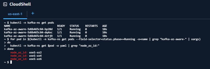
Verify that Availability Zone Ids have been injected into the pods
for pod in $(kubectl -n kafka-ns get pods --field-selector=status.phase==Running -o=name | grep "pod/kafka-az-aware-" | xargs)
do
  kubectl -n kafka-ns get "$pod" -o yaml | grep "node_az_id:"
done
Your output should look similar to:
node_az_id: use1-az2
node_az_id: use1-az4
node_az_id: use1-az6
Or:

Select a pod id from the output of the get pods command and shell-in to it.
kubectl -n kafka-ns exec -it POD_ID -- sh
The output of the get $pod command matches the order of results from the get pods command. This matching will help you understand what Availability Zone your pod is running in so you can compare it to log outputs later.
After you’ve connected to your pod, run the Kafka consumer:
"${KAFKA_BIN}"/kafka-console-consumer.sh \
  --bootstrap-server  "${BootstrapServerString}" \
  --consumer.config  "${KAFKA_CONFIG}"/client.properties \
  --topic "${MSK_TOPIC}" \
  --from-beginning /tmp/non-rack-aware-consumer.log 2>&1 &
Similar to before, this command will dump all the resulting logs into the file, rack-aware-consumer.log. You create a new file so there’s no overlap between the Kafka consumers you’ve run. There’s a lot of information in those logs, and we encourage you to open them and take a deeper look. If you want to see the rack awareness of your EKS pod in action, run the following command to tail the file to view fetch request results to the MSK cluster. You can observe a handful of meaningful logs to review here as the consumer access various partitions of the Kafka topic:
grep -E "DEBUG.*Added read_uncommitted fetch request for partition MSK-AZ-Aware-Topic-[0-9]+" /tmp/rack-aware-consumer.log | tail -5
Observe your log output, which should look similar to the following:
[2025-03-13 00:47:51,695] DEBUG [Consumer clientId=console-consumer, groupId=console-consumer-86303] Added read_uncommitted fetch request for partition MSK-AZ-Aware-Topic-5 at position FetchPosition{offset=527, offsetEpoch=Optional[0], currentLeader=LeaderAndEpoch{leader=Optional[b-1.mskazaware.hxrzlh.c6.kafka.us-east-1.amazonaws.com:9098 (id: 1 rack: use1-az4)], epoch=0}} to node b-2.mskazaware.hxrzlh.c6.kafka.us-east-1.amazonaws.com:9098 (id: 2 rack: use1-az6) (org.apache.kafka.clients.consumer.internals.AbstractFetch)
[2025-03-13 00:47:51,695] DEBUG [Consumer clientId=console-consumer, groupId=console-consumer-86303] Added read_uncommitted fetch request for partition MSK-AZ-Aware-Topic-4 at position FetchPosition{offset=509, offsetEpoch=Optional[0], currentLeader=LeaderAndEpoch{leader=Optional[b-3.mskazaware.hxrzlh.c6.kafka.us-east-1.amazonaws.com:9098 (id: 3 rack: use1-az2)], epoch=0}} to node b-2.mskazaware.hxrzlh.c6.kafka.us-east-1.amazonaws.com:9098 (id: 2 rack: use1-az6) (org.apache.kafka.clients.consumer.internals.AbstractFetch)
[2025-03-13 00:47:51,695] DEBUG [Consumer clientId=console-consumer, groupId=console-consumer-86303] Added read_uncommitted fetch request for partition MSK-AZ-Aware-Topic-3 at position FetchPosition{offset=527, offsetEpoch=Optional[0], currentLeader=LeaderAndEpoch{leader=Optional[b-2.mskazaware.hxrzlh.c6.kafka.us-east-1.amazonaws.com:9098 (id: 2 rack: use1-az6)], epoch=0}} to node b-2.mskazaware.hxrzlh.c6.kafka.us-east-1.amazonaws.com:9098 (id: 2 rack: use1-az6) (org.apache.kafka.clients.consumer.internals.AbstractFetch)
[2025-03-13 00:47:51,695] DEBUG [Consumer clientId=console-consumer, groupId=console-consumer-86303] Added read_uncommitted fetch request for partition MSK-AZ-Aware-Topic-2 at position FetchPosition{offset=522, offsetEpoch=Optional[0], currentLeader=LeaderAndEpoch{leader=Optional[b-1.mskazaware.hxrzlh.c6.kafka.us-east-1.amazonaws.com:9098 (id: 1 rack: use1-az4)], epoch=0}} to node b-2.mskazaware.hxrzlh.c6.kafka.us-east-1.amazonaws.com:9098 (id: 2 rack: use1-az6) (org.apache.kafka.clients.consumer.internals.AbstractFetch)
[2025-03-13 00:47:51,695] DEBUG [Consumer clientId=console-consumer, groupId=console-consumer-86303] Added read_uncommitted fetch request for partition MSK-AZ-Aware-Topic-1 at position FetchPosition{offset=533, offsetEpoch=Optional[0], currentLeader=LeaderAndEpoch{leader=Optional[b-3.mskazaware.hxrzlh.c6.kafka.us-east-1.amazonaws.com:9098 (id: 3 rack: use1-az2)], epoch=0}} to node b-2.mskazaware.hxrzlh.c6.kafka.us-east-1.amazonaws.com:9098 (id: 2 rack: use1-az6) (org.apache.kafka.clients.consumer.internals.AbstractFetch)
[2025-03-13 00:47:51,695] DEBUG [Consumer clientId=console-consumer, groupId=console-consumer-86303] Added read_uncommitted fetch request for partition MSK-AZ-Aware-Topic-0 at position FetchPosition{offset=520, offsetEpoch=Optional[0], currentLeader=LeaderAndEpoch{leader=Optional[b-2.mskazaware.hxrzlh.c6.kafka.us-east-1.amazonaws.com:9098 (id: 2 rack: use1-az6)], epoch=0}} to node b-2.mskazaware.hxrzlh.c6.kafka.us-east-1.amazonaws.com:9098 (id: 2 rack: use1-az6) (org.apache.kafka.clients.consumer.internals.AbstractFetch)
For each log line, you can now observe two rack: values. The first rack: value shows the current leader, the second rack: shows the rack that is being used to fetch messages.
For example, look at MSK-AZ-Aware-Topic-5. The leader is identified as rack: use1-az4, but the fetch request is sent to use1-az6 as indicated by to node b-2.mskazaware.hxrzlh.c6.kafka.us-east-1.amazonaws.com:9098 (id: 2 rack: use1-az6) (org.apache.kafka.clients.consumer.internals.AbstractFetch)
You’ll notice something similar in all other log lines. The fetch is always to the broker in use1-az6, which maps to our expectation, given the pod we connected to was in this Availability Zone.
Congratulations! You’re consuming from the closest replica on Amazon EKS.
Clean Up
Delete the deployment when finished:
kubectl -n kafka-ns delete -f kafka-az-aware.yaml
To delete the EKS Pod Identity association:
eksctl delete podidentityassociation \
--cluster ${EKS_CLUSTER_NAME} \
--namespace kafka-ns \
--service-account-name kafka-sa
To delete the IAM policy:
aws iam delete-policy \
  --policy-arn arn:aws:iam::"${AWS_ACCOUNT}":policy/MSK-AZ-Aware-Policy
To delete the EKS cluster:
eksctl delete cluster -n ${EKS_CLUSTER_NAME} --disable-nodegroup-eviction
If you followed along with this post using the Amazon MSK Data Generator, be sure to delete your deployment so it’s no longer attempting to generate and send data after you delete the rest of your resources.
Clean up will depend on which deployment option you used. To read more about the deployment options and the resources created for the Amazon MSK Data Generator, refer to Getting Started in the GitHub repository.
Creating an MSK cluster was a prerequisite of this post, and if you’d like to clean up the MSK cluster as well, you can use the following command:
aws kafka delete-cluster --cluster-arn "${MSK_CLUSTER_ARN}"
There is no additional cost to using AWS CloudShell, but if you’d like to delete your shell, refer to the Delete a shell session home directory in the AWS CloudShell User Guide.
Conclusion
Apache Kafka nearest replica fetching, or rack awareness, is a strategic cost-optimization technique. By implementing it for Amazon MSK consumers on Amazon EKS, you can significantly reduce cross-zone traffic costs while maintaining robust, distributed streaming architectures. Open source tools such as Kyverno can simplify complex configuration challenges and drive meaningful savings.The solution we’ve demonstrated provides a powerful, repeatable approach to dynamically injecting Availability Zone information into Kubernetes pods, optimize Kafka consumer routing, and minimize reduce transfer costs.
Additional resources
To learn more about rack awareness with Amazon MSK, refer to Reduce network traffic costs of your Amazon MSK consumers with rack awareness.
About the authors
 Austin Groeneveld is a Streaming Specialist Solutions Architect at Amazon Web Services (AWS), based in the San Francisco Bay Area. In this role, Austin is passionate about helping customers accelerate insights from their data using the AWS platform. He is particularly fascinated by the growing role that data streaming plays in driving innovation in the data analytics space. Outside of his work at AWS, Austin enjoys watching and playing soccer, traveling, and spending quality time with his family.
Farooq Ashraf is a Senior Solutions Architect at AWS, specializing in SaaS, Generative AI, and MLOps. He is passionate about blending multi-tenant SaaS concepts with Cloud services to innovate scalable solutions for the digital enterprise, and has several blog posts, and workshops to his credit.
 Gagan Brahmi is a Specialist Senior Solutions Architect at Amazon Web Services (AWS), specializing in Data Analytics and AI/ML solutions. With over 20 years in information technology, he helps customers architect scalable, high-performance analytics platforms using distributed data processing, real-time streaming technologies, and machine learning services on AWS. When not designing cloud solutions, Gagan enjoys exploring new places with his family.
 Arun Shanmugam is a Senior Analytics Solutions Architect at AWS, with a focus on building modern data architecture. He has been successfully delivering scalable data analytics solutions for customers across diverse industries. Outside of work, Arun is an avid outdoor enthusiast who actively engages in CrossFit, road biking, and cricket.
 George Oakes is a Senior Hybrid Solutions Architect at AWS, with a focus on edge, on-premise, and low latency architectures. He has been successfully delivering scalable hybrid AWS solutions for customers across diverse industries. Outside of work, George is an avid outdoor enthusiast who enjoys hiking and visiting parks and UNESCO sites around.
 Pathik Shah is a Sr. Analytics Architect on Amazon Athena. He joined AWS in 2015 and has been focusing in the big data analytics space since then, helping customers build scalable and robust solutions using AWS Analytics services.
 Aritra Gupta is a Senior Technical Product Manager on the Amazon S3 team at Amazon Web Services. He helps customers build and scale data lakes. Based in Seattle, he likes to play chess and badminton in his spare time.
 Jaydev Nath is a Solutions Architect at AWS, where he works with ISV customers to build secure, scalable, reliable, and cost-efficient cloud solutions. He brings strong expertise in building SaaS architecture on AWS with a focus on Generative AI and data analytics technologies to help deliver practical, valuable business outcomes for customers.
 David John Chakram is a Principal Solutions Architect at AWS. He specializes in building data platforms and architecting seamless data ecosystems. With a profound passion for databases, data analytics, and machine learning, he excels at transforming complex data challenges into innovative solutions and driving businesses forward with data-driven insights.
 Sharmila Shanmugam is a Solutions Architect at Amazon Web Services. She is passionate about solving the customers’ business challenges with technology and automation and reduce the operational overhead. In her current role, she helps customers across industries in their digital transformation journey and build secure, scalable, performant and optimized workloads on AWS.
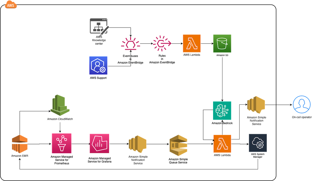


 Tomohiro Tanaka is a Senior Cloud Support Engineer at Amazon Web Services (AWS). He’s passionate about helping customers use Apache Iceberg for their data lakes on AWS. In his free time, he enjoys a coffee break with his colleagues and making coffee at home.
 Noritaka Sekiyama is a Principal Big Data Architect with AWS Analytics services. He’s responsible for building software artifacts to help customers. In his spare time, he enjoys cycling on his road bike.
 Sandeep Adwankar is a Senior Product Manager at Amazon Web Services (AWS). Based in the California Bay Area, he works with customers around the globe to translate business and technical requirements into products customers can use to improve how they manage, secure, and access data.
 Siddharth Padmanabhan Ramanarayanan is a Senior Software Engineer on the AWS Glue and AWS Lake Formation team, where he focuses on building scalable distributed systems for data analytics workloads. He is passionate about helping customers optimize their cloud infrastructure for performance and cost efficiency.
 Jon Handler is Director of Solutions Architecture for Search Services at Amazon Web Services, based in Palo Alto, CA. Jon works closely with OpenSearch and Amazon OpenSearch Service, providing help and guidance to a broad range of customers who have generative AI, search, and log analytics workloads for OpenSearch. Prior to joining AWS, Jon’s career as a software developer included four years of coding a large-scale, eCommerce search engine. Jon holds a Bachelor of the Arts from the University of Pennsylvania, and a Master of Science and a Ph. D. in Computer Science and Artificial Intelligence from Northwestern University.
 Arjun Kumar Giri is a Principal Engineer at AWS working on the OpenSearch Project. He primarily works on OpenSearch’s artificial intelligence and machine learning (AI/ML) and semantic search features. He is passionate about AI, ML, and building scalable systems.
 Siddhant Gupta is a Senior Product Manager (Technical) at AWS, spearheading AI innovation within the OpenSearch Project from Hyderabad, India. With a deep understanding of artificial intelligence and machine learning, Siddhant architects features that democratize advanced AI capabilities, enabling customers to harness the full potential of AI without requiring extensive technical expertise. His work seamlessly integrates cutting-edge AI technologies into scalable systems, bridging the gap between complex AI models and practical, user-friendly applications.
 Smita Singh is a Senior Solutions Architect at AWS. She focuses on defining technical strategic vision and works on architecture, design, and implementation of modern, scalable platforms for large-scale global enterprises and SaaS providers. She is a data, analytics, and generative AI enthusiast and is passionate about building innovative, highly scalable, resilient, fault-tolerant, self-healing, multi-tenant platform solutions and accelerators.
 Dipayan Sarkar is a Specialist Solutions Architect for Analytics at AWS, where he helps customers modernize their data platform using AWS analytics services. He works with customers to design and build analytics solutions, enabling businesses to make data-driven decisions.
 Ezat Karimi is a Senior Solutions Architect at AWS, based in Austin, TX. Ezat specializes in designing and delivering modernization solutions and strategies for database applications. Working closely with multiple AWS teams, Ezat helps customers migrate their database workloads to the AWS Cloud.
 Amit Maindola is a Senior Data Architect focused on data engineering, analytics, and AI/ML at Amazon Web Services. He helps customers in their digital transformation journey and enables them to build highly scalable, robust, and secure cloud-based analytical solutions on AWS to gain timely insights and make critical business decisions.
 Arghya Banerjee is a Sr. Solutions Architect at AWS in the San Francisco Bay Area, focused on helping customers adopt and use the AWS Cloud. He is focused on big data, data lakes, streaming and batch analytics services, and generative AI technologies.
 Melody Yang is a Principal Analytics Architect for Amazon EMR at AWS. She is an experienced analytics leader working with AWS customers to provide best practice guidance and technical advice in order to assist their success in data transformation. Her areas of interests are open-source frameworks and automation, data engineering and DataOps.
 Gaurav Parekh is a Solutions Architect at AWS, specializing in generative AI and data analytics, with extensive experience building production AI systems on AWS.
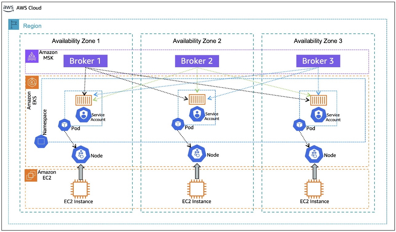
 Austin Groeneveld is a Streaming Specialist Solutions Architect at Amazon Web Services (AWS), based in the San Francisco Bay Area. In this role, Austin is passionate about helping customers accelerate insights from their data using the AWS platform. He is particularly fascinated by the growing role that data streaming plays in driving innovation in the data analytics space. Outside of his work at AWS, Austin enjoys watching and playing soccer, traveling, and spending quality time with his family.
 Farooq Ashraf is a Senior Solutions Architect at AWS, specializing in SaaS, Generative AI, and MLOps. He is passionate about blending multi-tenant SaaS concepts with Cloud services to innovate scalable solutions for the digital enterprise, and has several blog posts, and workshops to his credit.

 Mohit Dawar is a Senior Software Engineer at Amazon Web Services (AWS) working on Amazon DataZone. Over the past 3 years, he has led efforts around the core metadata catalog, generative AI–powered metadata curation, and lineage visualization. He enjoys working on large-scale distributed systems, experimenting with AI to improve user experience, and building tools that make data governance feel effortless. Connect with him on LinkedIn:
  Jose Romero is a Senior Solutions Architect for Startups at Amazon Web Services (AWS) based in Austin, TX, US. He is passionate about helping customers architect modern platforms at scale for data, AI, and ML. As a former senior architect in AWS Professional Services, he enjoys building and sharing solutions for common complex problems so that customers can accelerate their cloud journey and adopt best practices. Connect with him on LinkedIn:

 Brody Pearman is a Senior Cloud Support Engineer at Amazon Web Services (AWS). He’s passionate about helping customers use AWS Glue ETL to transform and create their data lakes on AWS while maintaining high data quality. In his free time, he enjoys watching football with his friends and walking his dog.
 Shiv Narayanan is a Technical Product Manager for AWS Glue’s data management capabilities like data quality, sensitive data detection and streaming capabilities. Shiv has over 20 years of data management experience in consulting, business development and product management.
 Shriya Vanvari is a Software Developer Engineer in AWS Glue. She is passionate about learning how to build efficient and scalable systems to provide better experience for customers. Outside of work, she enjoys reading and chasing sunsets.
 Narayani Ambashta is an Analytics Specialist Solutions Architect at AWS, focusing on the automotive and manufacturing sector, where she guides strategic customers in developing modern data and AI strategies. With over 15 years of cross-industry experience, she specializes in big data architecture, real-time analytics, and AI/ML technologies, helping organizations implement modern data architectures. Her expertise spans across lakehouse architecture, generative AI, and IoT platforms, enabling customers to drive digital transformation initiatives. When not architecting modern solutions, she enjoys staying active through sports and yoga.
 Mohammad Sabeel Mohammad Sabeel is a Senior Cloud Support Engineer at Amazon Web Services (AWS) with over 14 years of experience in Information Technology (IT). As a member of the Technical Field Community (TFC) Analytics team, he is a Subject matter expert in Analytics services AWS Glue, Amazon Managed Workflows for Apache Airflow (MWAA), and Amazon Athena services. Sabeel provides expert guidance and technical support to enterprise and strategic customers, helping them optimize their data analytics solutions and overcome complex challenges. With deep subject matter expertise he enables organizations to build scalable, efficient, and cost-effective data processing pipelines.
 Indira Balakrishnan Indira Balakrishnan is a Principal Solutions Architect in the Amazon Web Services (AWS) Analytics Specialist Solutions Architect (SA) Team. She helps customers build cloud-based Data and AI/ML solutions to address business challenges. With over 25 years of experience in Information Technology (IT), Indira actively contributes to the AWS Analytics Technical Field community, supporting customers across various Domains and Industries. Indira participates in Women in Engineering and Women at Amazon tech groups to encourage girls to pursue STEM path to enter careers in IT. She also volunteers in early career mentoring circles.
 Gregory Knowles is a data and AI specialist solution architect at AWS, focusing on the UK public sector. With extensive experience in cloud-based architectures, Greg guides public sector customers in implementing modern data solutions. His expertise spans governance, analytics, and AI/ML. Greg’s passion lies in accelerating transformation and innovation to improve productivity and outcomes. He has successfully led projects that moved data systems into the cloud, adopted new data architectures, and implemented AI at scale in production.
 Abhinav Tripathy is a Software Engineer and Security Guardian at AWS, where he develops Amazon Q generative SQL by combining machine learning, databases, and web systems. Abhinav is passionate about building scalable web systems from scratch that solve real customer challenges. Outside of work, he enjoys traveling, watching soccer, and playing badminton.
 Erol Murtezaoglu is a Technical Product Manager at AWS, is an inquisitive and enthusiastic thinker with a drive for self-improvement and learning. He has a strong and proven technical background in software development and architecture, balanced with a drive to deliver commercially successful products. Erol highly values the process of understanding customer needs and problems, in order to deliver solutions that exceed expectations.


 Ashok Padmanabhan is a Sr. IoT Data Architect with AWS Professional Services. Ashok primarily works with manufacturing and automotive customers to design and build Industry 4.0 solutions.
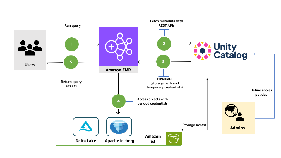

 Venkatavaradhan (Venkat) Viswanathan is a Global Partner Solutions Architect at Amazon Web Services. Venkat is a Technology Strategy Leader in Data, AI, ML, generative AI, and Advanced Analytics. Venkat is a Global SME for Databricks and helps AWS customers design, build, secure, and optimize Databricks workloads on AWS.
 Srividya Parthasarathy is a Senior Big Data Architect on the AWS Lake Formation team. She works with the product team and customers to build robust features and solutions for their analytical data platform. She enjoys building data mesh solutions and sharing them with the community.
 Ramkumar Nottath is a Principal Solutions Architect at AWS focusing on Analytics services. He enjoys working with various customers to help them build scalable, reliable big data and analytics solutions. His interests extend to various technologies such as analytics, data warehousing, streaming, data governance, and machine learning. He loves spending time with his family and friends.
 John Spencer is a Product Manager at Databricks, dedicated to making Unity Catalog work seamlessly with customers’ ecosystems of tools and platforms so they can easily access, govern, and use their data.
 Sreeram Thoom is a Specialist Solutions Architect at Databricks helping customers design secure, scalable applications on the Data Lakehouse.
 Dipankar Kushari is a specialist solutions architect at Databricks helping customer architect and build secured applications on Data Lakehouse.


 Manabu McCloskey is a Solutions Architect at Amazon Web Services. He focuses on contributing to open source application delivery tooling and works with AWS strategic customers to design and implement enterprise solutions using AWS resources and open source technologies. His interests include Kubernetes, GitOps, Serverless, and Souls Series.
 Vara Bonthu is a Principal Open Source Specialist SA leading Data on EKS and AI on EKS at AWS, driving open source initiatives and helping AWS customers to diverse organizations. He specializes in open source technologies, data analytics, AI/ML, and Kubernetes, with extensive experience in development, DevOps, and architecture. Vara focuses on building highly scalable data and AI/ML solutions on Kubernetes, enabling customers to maximize cutting-edge technology for their data-driven initiatives
 Andrew Kim is a Software Development Engineer at AWS Glue, with a deep passion for distributed systems architecture and AI-driven solutions, specializing in intelligent data integration workflows and cutting-edge feature development on Apache Spark. Andrew focuses on re-inventing and simplifying solutions to complex technical problems, and he enjoys creating web apps and producing music in his free time.
 Shubham Mehta is a Senior Product Manager at AWS Analytics. He leads generative AI feature development across services such as AWS Glue, Amazon EMR, and Amazon MWAA, using AI/ML to simplify and enhance the experience of data practitioners building data applications on AWS.
 Kartik Panjabi is a Software Development Manager on the AWS Glue team. His team builds generative AI features for the Data Integration and distributed system for data integration.
 Mohit Saxena is a Senior Software Development Manager on the AWS Data Processing Team (AWS Glue and Amazon EMR). His team focuses on building distributed systems to enable customers with new AI/ML-driven capabilities to efficiently transform petabytes of data across data lakes on Amazon S3, databases and data warehouses on the cloud.
 Shubham Mehta is a Senior Product Manager at AWS Analytics. He leads generative AI feature development across services such as AWS Glue, Amazon EMR, and Amazon MWAA, using AI/ML to simplify and enhance the experience of data practitioners building data applications on AWS.
 Vaibhav Naik is a software engineer at AWS Glue, passionate about building robust, scalable solutions to tackle complex customer problems. With a keen interest in generative AI, he likes to explore innovative ways to develop enterprise-level solutions that harness the power of cutting-edge AI technologies.
 Liyuan Lin is a Software Engineer at AWS Glue, where she works on building generative AI and data integration tools to help customers solve their data challenges. She specializes in developing solutions that combine AI capabilities with data integration workflows, making it easier for customers to manage and transform their data effectively.
 Arun A K is a Big Data Solutions Architect with AWS. He works with customers to provide architectural guidance for running analytics solutions on the cloud. In his free time, Arun loves to enjoy quality time with his family.
 Sarath Krishnan is a Senior Solutions Architect with Amazon Web Services. He is passionate about enabling enterprise customers on their digital transformation journey. Sarath has extensive experience in architecting highly available, scalable, cost-effective, and resilient applications on the cloud. His area of focus includes DevOps, machine learning, MLOps, and generative AI.
 Pradeep Patel is a Software Development Manager on the AWS Data Processing Team (AWS Glue and Amazon EMR). His team focuses on building distributed systems to enable seamless Spark Code Transformation using AI.
 Mohit Saxena is a Senior Software Development Manager on the AWS Data Processing Team (AWS Glue and Amazon EMR). His team focuses on building distributed systems to enable customers with new AI/ML-driven capabilities to efficiently transform petabytes of data across data lakes on Amazon S3, databases and data warehouses on the cloud.