Post Syndicated from Ezat Karimi original https://aws.amazon.com/blogs/big-data/workload-management-in-opensearch-based-multi-tenant-centralized-logging-platforms/
Modern architectures use many different technologies to achieve their goals. Service-oriented architectures, cloud services, distributed tracing, and more create streams of telemetry and other signal data. Each of these data streams becomes a tenant in your logging backend. If your company runs more than one application, the IT team will frequently centralize the storage and processing of log data, making each application a tenant in the overall observability system.
When you use Amazon OpenSearch Service to store and analyze log data, whether as a developer or an IT admin, you must balance these tenants to make sure you deliver the resources to each tenant so they can ingest, store, and query their data. In this post, we present a multi-layered workload management framework with a rules-based proxy and OpenSearch workload management that can effectively address these challenges.
Example use case
In this post, we discuss GlobalLog, a fictional company supporting healthcare, finance, retail, security, and internal tenants, that built a centralized logging system with OpenSearch Service. Each tenant has unique logging patterns based on their business requirements. Financial tenants generate complex, high-volume queries, healthcare tenants focus on compliance with moderate volume logs and queries, and retail tenants experience seasonal spikes with heavy dashboard usage. Internal operation has steady, low-volume logs and infrequent, simple queries. Security monitoring has a constant, high-volume presence throughout the system.
As the GlobalLog’s tenants scaled, operational challenges emerged: high-priority tenant performance suffered during peak hours, resource-intensive queries caused node crashes, and unpredictable traffic created instability. Limited visibility into tenant resource usage complicated troubleshooting and cross-domain security investigations. The platform required robust handling of varied workload patterns and peak usage times, strong performance isolation to prevent tenant interference, and scalability to manage 30% annual data growth.
Solution overview
GlobalLog implemented a comprehensive workload management strategy to handle the diverse demands of its tenants. The solution manages the tenancy with a tiered tenant placement, a rule-based proxy layer that shapes incoming traffic based on the tenant profile and the status of the OpenSearch cluster, and an OpenSearch workload management plugin that provides granular resource governance, allocating resources such as CPU and memory proportionally to each tenant’s tier. The monitoring component provides the intelligence that the solution needs to do its assessment and make reactive and proactive scaling and performance-related decisions by adjusting the traffic governance rules and policies in a timely manner.
The following diagram illustrates the architecture.
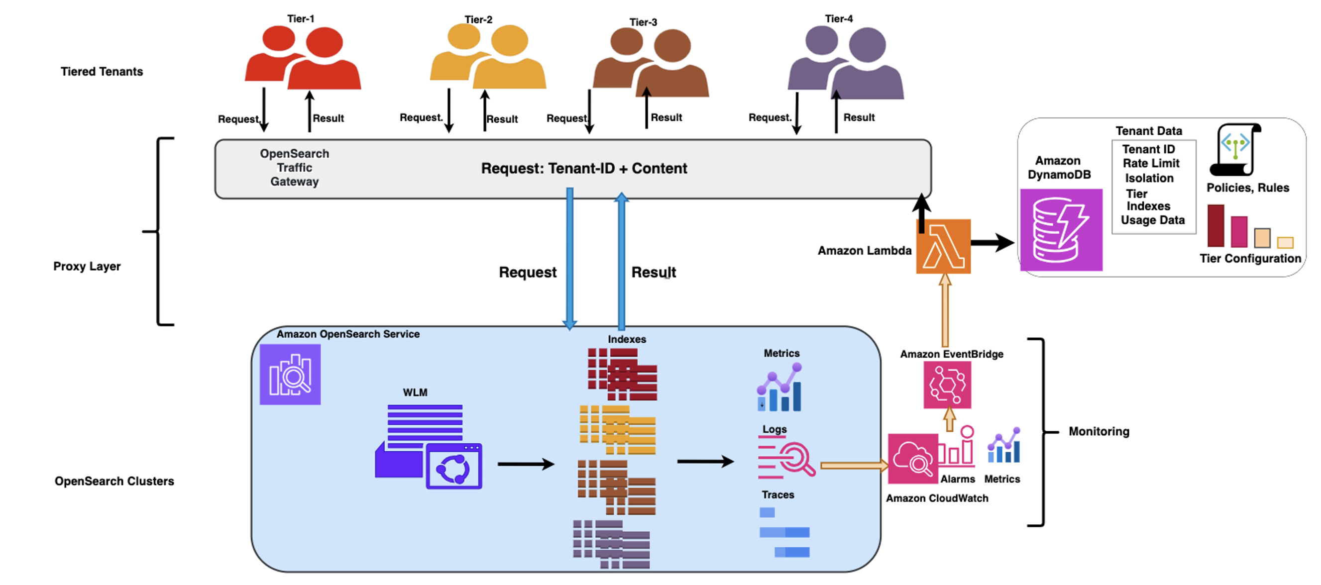
GlobalLog multi tier workload management
Tenant tiering and placement
GlobalLog categorized tenants into four tiers based on their logging requirements (volume, retention, query frequency) and allocated resources accordingly. The tiering system, enforced through the integrated proxy layer and OpenSearch workload management, prevents resource over-allocation while making sure service levels match business priorities. The specification for each tier is detailed in the following table.
| Tier | SLA | Resources | Limits | Behavior |
|
Tier 1 (Enterprise Critical) High-volume complex queries (over 100 concurrent) |
24/7 SLA with 99.99% availability |
50% CPU 50% Memory |
100 concurrent requests 20 MB request size 180-second timeout |
Priority query routing and dedicated search threads |
|
Tier 2 (Business Critical) Moderate volume compliance-oriented queries |
Business hours SLA with 99.9% availability |
30% CPU 25% memory |
50 concurrent requests 10 MB request size 120-second timeout |
Compliance-optimized search pipelines |
|
Tier 3 (Business Standard) Variable volume dashboard-heavy usage |
Standard business hours support no SLA |
10% CPU 20% Memory |
25 concurrent requests 5 MB request size 60-second timeout |
Burst capacity for seasonal peaks |
|
Tier 4 (Basic) Internal IT operations development environments |
Best-effort support no SLA |
10% CPU 5%Memory |
10 concurrent requests, 2 MB request size 30-second timeout |
Automated query optimization for efficiency Operations, seasonal businesses |
GlobalLog’s integrated architecture streamlines its cost allocation and resource distribution model. Financial industry tenants pay premium rates for their guaranteed high-performance resources, effectively subsidizing the infrastructure that supports more variable workloads. These tenants are categorized into Tier 1. Healthcare tenants benefit from isolation that enforces compliance without bearing the full cost of dedicated infrastructure. These tenants are categorized into Tier 2. Retail tenants are categorized into Tier 3 because they appreciate the elastic capacity during peak seasons without maintaining excess capacity year-round. Tier 4 includes the administrative tenants with access to enterprise-grade logging at affordable rates through efficient resource sharing.
This balanced ecosystem helps GlobalLog maintain profitability while delivering appropriate service levels to every tenant regardless of their industry-specific workload characteristics.
In the next sections, we discuss GlobalLog’s workload management system.
Proxy layer
GlobalLog’s continuous feedback loop architecture creates a dynamic ecosystem that optimizes resource allocation across diverse tenant workloads in OpenSearch Service. Rather than depending on static configurations, the architecture monitors performance metrics and tenant usage patterns to drive scaling and remediation decisions. This makes sure the system evolves as workloads change over time.
The proxy layer core component is the OpenSearch Traffic Gateway, which functions as an intermediary between clients and OpenSearch clusters. It features the following key capabilities:
- Rule-based traffic shaping through pattern matching for request paths and parameters
- Metrics for resource cost allocation
- Traffic replay
GlobalLog expanded the capabilities of their OpenSearch Traffic Gateway through a comprehensive set of enhancements focused on centralization, dynamism, and adaptability. At the core of this evolution, they used Amazon DynamoDB as the centralized repository for critical gateway data. This central database houses the complete ecosystem of rules, policies, and tenant profiles, alongside crucial operational data including metrics, usage patterns, SLA requirements, tier configurations, and real-time cluster status information.
Beyond this centralization effort, GlobalLog transformed the gateway with a dynamic mechanism capable of real-time adjustments and responsive decision-making. This architectural shift allows the gateway to react intelligently to changing conditions rather than following predetermined pathways.
Additionally, GlobalLog implemented an adaptive rule system with sophisticated contextual awareness. The system now activates specific rules based on current cluster states and tenant usage patterns, enabling precise resource allocation and protection mechanisms that respond to actual conditions rather than hypothetical scenarios. The system implements time-based rule scheduling, providing flexibility by allowing different limits and policies to automatically engage during specific periods such as maintenance windows. This provides optimal performance while accommodating necessary system operations.
The solution implements a continuous feedback loop between the monitoring system, the OpenSearch cluster, and the proxy layer, where the flow of performance metrics and tenant usage patterns drive automated, rule-based scaling and optimization decisions, helping the system evolve as workloads change over time. In this architecture, Amazon EventBridge triggers an AWS Lambda function when predefined criteria are met (for example, an anomaly is detected in OpenSearch Service), resulting in the Lambda function taking steps to remediate the issues by adjusting the traffic shaping rules and uploading them to the OpenSearch Traffic Gateway. To stabilize the feedback loop, GlobalLog took the following steps:
- Added dampening mechanisms to prevent rapid rule changes
- Implemented gradual adjustment patterns instead of binary switches
- Created circuit breakers for automatic fallback to baseline rules
OpenSearch workload management layer
GlobalLog implemented tenant-level admission control and reactive query management through OpenSearch workload management. The system uses workload management to define resource limits, based on tenant criticality, providing efficient resource allocation and preventing bottlenecks.
A key component of OpenSearch’s workload management is its workload groups. A workload group refers to a logical grouping of queries, typically used for managing resources and prioritizing workloads. GlobalLog uses workload groups to manage resource allocation based on the previously defined tenant tiers. Enterprise-critical workloads receive substantial CPU and memory guarantees, providing consistent performance for financial operations. Business Critical tenants operate with moderate resource guarantees, and Standard and Basic tiers function with more constrained resources, reflecting their lower priority status. The following example shows the workload group setup for Enterprise Critical and Business Critical tiers:
OpenSearch responds with the set resource limits and the ID for the workload group for Enterprise Critical tier tenants:
To use a workload group, use the following code:
Real-world use cases
In this section, we discuss two scenarios where GlobalLog’s workload management system helped the company overcome various challenges.
Scenario 1: Security incident response
During a critical security incident, GlobalLog faced a complex challenge of managing simultaneous log access requests from multiple business units, each with different priority levels. At the highest tier were security and financial operations (Tier 1), followed by healthcare operations (Tier 2), retail operations (Tier 3), and internal operations (Tier 4).
At the proxy layer, GlobalLog gave precedence to security and financial tenant queries while implementing specific limitations for other units. Healthcare operations were capped at 15 concurrent queries, retail operations were restricted to 5 queries per minute, and internal operations had their date ranges narrowed.
OpenSearch workload management and the proxy layer played a crucial role by maintaining the security team’s query priority while managing resource pressure, including the cancellation of complex retail queries during high CPU usage.
Scenario 2: End-of-month reporting
During month-end reporting periods, GlobalLog successfully handled intensive analytical workloads from multiple tenants. The implementation of time-based rules proved particularly effective, with prioritizing Tier 4 tenants for batch reporting during regular end-of-month off-peak business hours. The following code shows an example of GlobalLog rules in this context. The first rule allows Tier 4 tenants to run reports during off-peak business hours, and the second rule denies Tier 4 tenants’ requests during business hours:
The system dynamically adjusted resource allocation for Tier 4 tenants for the off-peak hours (6:00 PM – 8:00 AM) using the OpenSearch workload management API.
This comprehensive approach proved highly successful in managing peak reporting periods, facilitating both system stability and optimal performance across all tenant tiers.
Conclusion
The integration of proxy-layer traffic shaping with the OpenSearch workload management plugin in a continuous feedback loop architecture achieved resiliency, stable performance, and fair resource allocation while supporting diverse business priorities. The implementation discussed in this post demonstrates that large-scale, multi-tenant logging environments can effectively serve diverse business needs on shared infrastructure while maintaining performance and cost-efficiency.
Try out these workload management techniques for your own use case and share your feedback and questions in the comments.
About the Authors
 Ezat Karimi is a Senior Solutions Architect at AWS, based in Austin, TX. Ezat specializes in designing and delivering modernization solutions and strategies for database applications. Working closely with multiple AWS teams, Ezat helps customers migrate their database workloads to the AWS Cloud.
 Jon Handler is a Senior Principal Solutions Architect at AWS based in Palo Alto, CA. Jon works closely with OpenSearch and Amazon OpenSearch Service, providing help and guidance to a broad range of customers who have vector, search, and log analytics workloads that they want to move to the AWS Cloud. Prior to joining AWS, Jon’s career as a software developer included 4 years of coding a large-scale, ecommerce search engine. Jon holds a Bachelor’s of the Arts from the University of Pennsylvania, and a Master’s of Science and a PhD in Computer Science and Artificial Intelligence from Northwestern University.
 Sohaib Katariwala is a Senior Specialist Solutions Architect at AWS focused on Amazon OpenSearch Service based out of Chicago, IL. His interests are in all things data and analytics. More specifically he loves to help customers use AI in their data strategy to solve modern day challenges.
 Mark Twomey is a Senior Solutions Architect at AWS focused on storage and data management. He enjoys working with customers to put their data in the right place, at the right time, for the right cost. Living in Ireland, Mark enjoys walking in the countryside, watching movies, and reading books.
 Sorabh Hamirwasia is a senior software engineer at AWS working on the OpenSearch Project. His primary interest include building cost optimized and performant distributed systems.
 Pallavi Priyadarshini is a Senior Engineering Manager at Amazon OpenSearch Service leading the development of high-performing and scalable technologies for search, security, releases, and dashboards.
 Bobby Mohammed is a Principal Product Manager at AWS leading the Search, GenAI, and Agentic AI product initiatives. Previously, he worked on products across the full lifecycle of machine learning, including data, analytics, and ML features on SageMaker platform, deep learning training and inference products at Intel.


 Ramon Lopez is a Principal Solutions Architect for Amazon QuickSight. With many years of experience building BI solutions and a background in accounting, he loves working with customers, creating solutions, and making world-class services. When not working, he prefers to be outdoors in the ocean or up on a mountain.
 Leonardo Gomez is a Principal Analytics Specialist Solutions Architect at AWS. He has over a decade of experience in data management, helping customers around the globe address their business and technical needs. Connect with him on

 Michael Torio is an Associate Specialist Solutions Architect at AWS focused on Amazon OpenSearch Service based out of Mountain View, CA. Michael enjoys helping customers leverage cloud technologies to solve their business challenges.
 Arjun Nambiar is a Product Manager with Amazon OpenSearch Service. He focuses on ingestion technologies that enable ingesting data from a wide variety of sources into Amazon OpenSearch Service at scale. Arjun is interested in large-scale distributed systems and cloud-centered technologies, and is based out of Seattle, Washington.
 Noritaka Sekiyama is a Principal Big Data Architect with AWS Analytics services. He’s responsible for building software artifacts to help customers. In his spare time, he enjoys cycling on his road bike.
 Tomohiro Tanaka is a Senior Cloud Support Engineer at Amazon Web Services. He’s passionate about helping customers use Apache Iceberg for their data lakes on AWS. In his free time, he enjoys a coffee break with his colleagues and making coffee at home.
 Peter Tsai is a Software Development Engineer at AWS, where he enjoys solving challenges in the design and performance of the AWS Glue runtime. In his leisure time, he enjoys hiking and cycling.
 Matt Su is a Senior Product Manager on the AWS Glue team. He enjoys helping customers uncover insights and make better decisions using their data with AWS Analytics services. In his spare time, he enjoys skiing and gardening.
 Sean McGeehan is a Software Development Engineer at AWS, where he builds features for the AWS Glue fulfillment system. In his leisure time, he explores his home of Philadelphia and work city of New York.


 Chiho Sugimoto is a Cloud Support Engineer on the AWS Big Data Support team. She is passionate about helping customers build data lakes using ETL workloads. She loves planetary science and enjoys studying the asteroid Ryugu on weekends.
 Saeed Barghi is a Sr. Specialist Solutions Architect at Amazon Web Services (AWS) specializing in architecting enterprise data platforms and AI solutions. Based in Melbourne, Australia, Saeed works with public sector customers in Australia and New Zealand and helps his customers build fit-for-purpose and future-proof data platforms and AI solutions.
 Miroslaw (Mick) Mioduszewski is the Director of Analytics at Revenue NSW Department of Customer service in NSW. He held multiple C-level roles in private and public companies as well as government, e.g. COO and CIO, as well as serving as company director. Mick holds computer science and business degrees, is a fellow of the Australian Institute of Company Directors and an industry fellow at the University of technology, Sydney.
 Moha Alsouli is a Public Sector Solutions Architect at Amazon Web Services (AWS) in Sydney. He is dedicated to supporting state and local government customers deliver citizen services, through solution design, reviews, optimisation, and architecture guidance. Moha is also specialising in generative artificial intelligence (AI) on AWS.


 Akira Mikami is a technical expert who played a central role in the FURUNO Data Platform (JuBuRaw) Construction Project at Furuno Electric Co., Ltd. Specializing in data platform construction and architecture, he led the implementation of cloud solutions utilizing AWS. He contributed to achieving efficient data management and strengthening team collaboration, leading the project to success.
 Junpei Ozono is a Sr. Go-to-market (GTM) Data & AI solutions architect at Amazon Web Services (AWS) in Japan. He drives technical market creation for data and AI solutions while collaborating with global teams to develop scalable GTM motions. He guides organizations in designing and implementing innovative data-driven architectures powered by AWS services, helping customers accelerate their cloud transformation journey through modern data and AI solutions. His expertise spans across modern data architectures including data mesh, data lakehouse, and generative AI, so customers can build scalable and innovative solutions on Amazon Web Services (AWS).
 Mitsuhiko Nishida is an Enterprise Solutions Architecture Automotive & Manufacturing Group Solutions Architect at Amazon Web Services (AWS) in Japan. He serves as a field Solutions Architect for manufacturing customers, helping them solve their business challenges. With expertise in generative AI and manufacturing IT, he guides the design and implementation of innovative solutions leveraging cutting-edge technologies. He supports manufacturing customers in building efficient architecture powered by AWS services to accelerate their cloud transformation journey and contribute to their digital transformation initiatives.


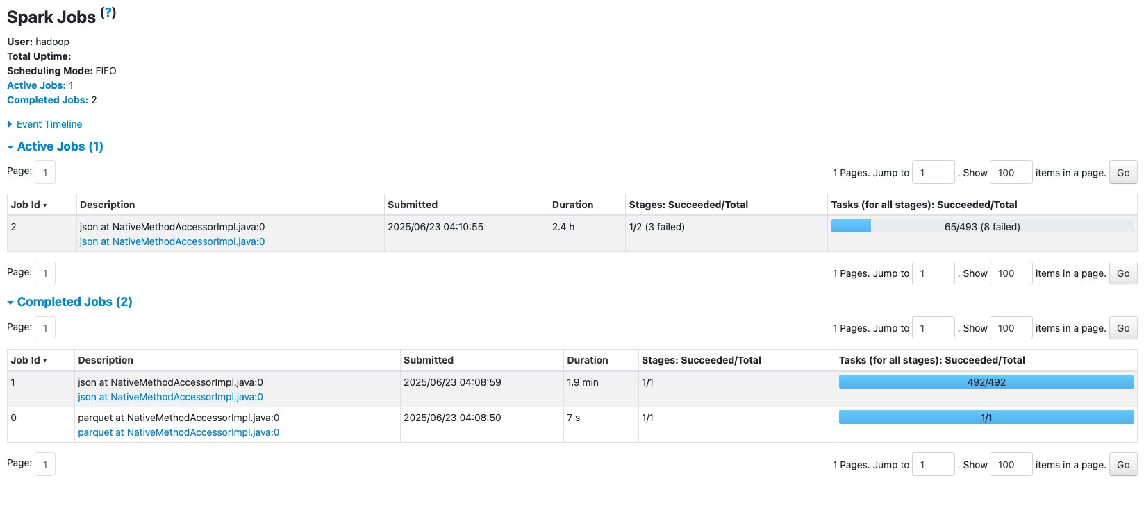
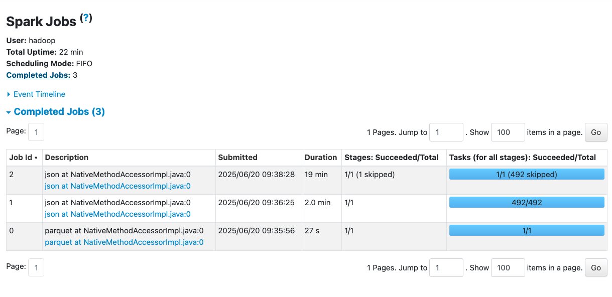
 The following screenshot shows an example of the Spark UI.
  The following screenshot shows an example of the driver logs.
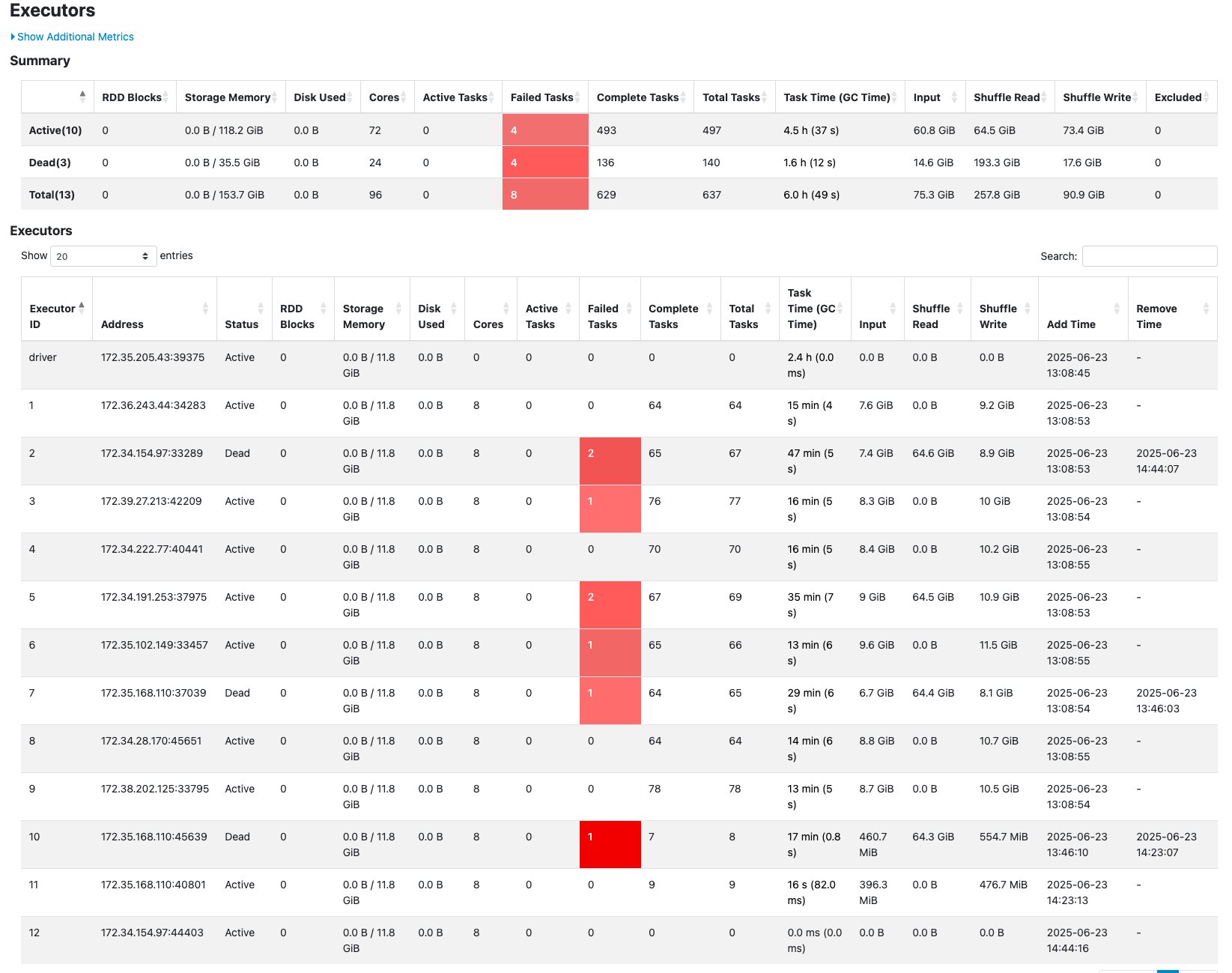
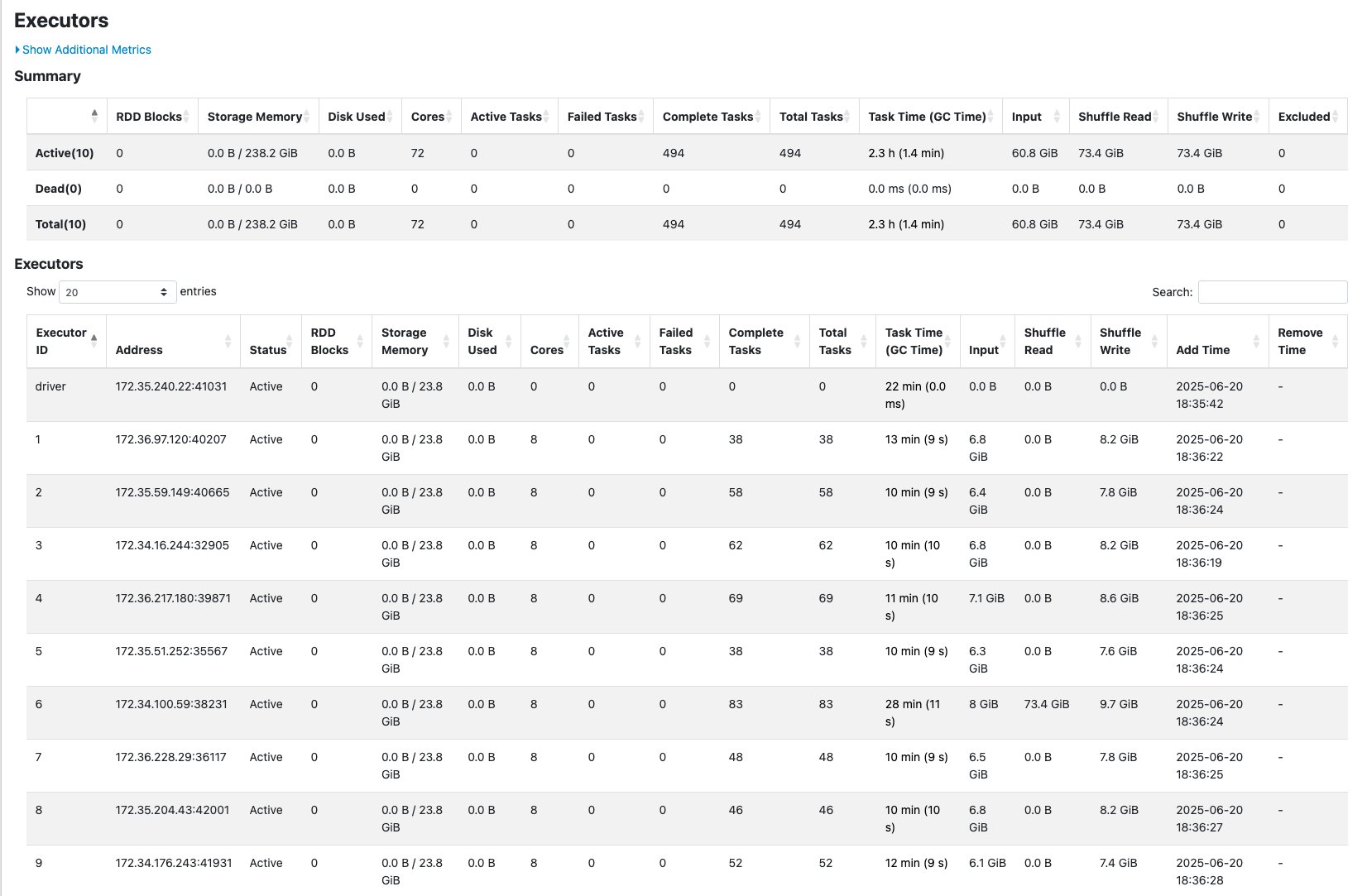
  The following screenshot shows the Executors tab, which provides access to the driver and executor logs.


 In the following example, we run some TPC-DS SQL statements that are used for performance and benchmarks:


 Amit Maindola is a Senior Data Architect focused on data engineering, analytics, and AI/ML at Amazon Web Services. He helps customers in their digital transformation journey and enables them to build highly scalable, robust, and secure cloud-based analytical solutions on AWS to gain timely insights and make critical business decisions.
 Abhilash is a senior specialist solutions architect at Amazon Web Services (AWS), helping public sector customers on their cloud journey with a focus on AWS Data and AI services. Outside of work, Abhilash enjoys learning new technologies, watching movies, and visiting new places.


 Enrique Salgado Hernández is a Senior Specialist Solutions Architect at AWS with more than 10 years of experience working in the cloud. He specializes in designing and implementing large-scale analytics architectures across various industry sectors. He is passionate about working with customers to solve their problems by supporting them during their cloud journey.
 Angel Conde Manjon is a Senior EMEA Data & AI PSA, based in Madrid. He previously worked on research related to data analytics and AI in diverse European research projects. In his current role, Angel helps partners develop businesses centered on data and AI.


 Swapna Bandla is a Senior Solutions Architect in the AWS Analytics Specialist SA Team. Swapna has a passion towards understanding customers data and analytics needs and empowering them to develop cloud-based well-architected solutions. Outside of work, she enjoys spending time with her family.
 Austin Groeneveld is a Streaming Specialist Solutions Architect at Amazon Web Services (AWS), based in the San Francisco Bay Area. In this role, Austin is passionate about helping customers accelerate insights from their data using the AWS platform. He is particularly fascinated by the growing role that data streaming plays in driving innovation in the data analytics space. Outside of his work at AWS, Austin enjoys watching and playing soccer, traveling, and spending quality time with his family.


 Srinivas Kandi is a Senior Architect at Stifel focusing on delivering the next generation of cloud data platform on AWS. Prior to joining Stifel, Srini was a delivery specialist in cloud data analytics at AWS helping several customers in their transformational journey into AWS cloud. In his free time, Srini likes to explore cooking, travel and learn new trends and innovations in AI and cloud computing.
 Hossein Johari is a seasoned data and analytics leader with over 25 years of experience architecting enterprise-scale platforms. As Lead and Senior Architect at Stifel Financial Corp. in St. Louis, Missouri, he spearheads initiatives in Data Platforms and Strategic Solutions, driving the design and implementation of innovative frameworks that support enterprise-wide analytics, strategic decision-making, and digital transformation. Known for aligning technical vision with business objectives, he works closely with cross-functional teams to deliver scalable, forward-looking solutions that advance organizational agility and performance.
 Ahmad Rawashdeh is a Senior Architect at Stifel Financial. He supports Stifel and its clients in designing, implementing, and building scalable and reliable data architectures on Amazon Web Services (AWS), with a strong focus on data lake strategies, database services, and efficient data ingestion and transformation pipelines.
 Lei Meng is a data architect at Stifel. His focus is working in designing and implementing scalable and secure data solutions on the AWS and helping Stifel’s cloud migration from on-premises systems.


 Bharav Patel is a Specialist Solution Architect, Analytics at Amazon Web Services. He primarily works on Amazon OpenSearch Service and helps customers with key concepts and design principles of running OpenSearch workloads on the cloud. Bharav likes to explore new places and try out different cuisines.
 Imtiaz (Taz) Sayed is the WW Tech Leader for Analytics at AWS. He enjoys engaging with the community on all things data and analytics. He can be reached through
  Chinmayi Narasimhadevara is a Senior Solutions Architect focused on Data Analytics and AI at AWS. She helps customers build advanced, highly scalable, and performant solutions.


 Ido Ziv is a DevOps team leader in Kaltura with over 6 years of experience. His hobbies include sailing and Kubernetes (but not at the same time).
 Roi Gamliel is a Senior Solutions Architect helping startups build on AWS. He is passionate about the OpenSearch Project, helping customers fine-tune their workloads and maximize results.
 Yonatan Dolan is a Principal Analytics Specialist at Amazon Web Services. He is located in Israel and helps customers harness AWS analytical services to use data, gain insights, and derive value.


 Ramesh H Singh is a Senior Product Manager Technical (External Services) at AWS in Seattle, Washington, currently with the Amazon SageMaker team. He is passionate about building high-performance ML/AI and analytics products that enable enterprise customers to achieve their critical goals using cutting-edge technology. Connect with him on
  Pradeep Misra is a Principal Analytics Solutions Architect at AWS. He works across Amazon to architect and design modern distributed analytics and AI/ML platform solutions. He is passionate about solving customer challenges using data, analytics, and AI/ML. Outside of work, Pradeep likes exploring new places, trying new cuisines, and playing board games with his family. He also likes doing science experiments, building LEGOs and watching anime with his daughters.
 Balaji Kumar Gopalakrishnan is a Principal Engineer at Amazon Finance Technology. He has been with Amazon since 2013, solving real-world challenges through technology that directly impact the lives of Amazon customers. Outside of work, Balaji enjoys hiking, painting, and spending time with his family. He is also a movie buff!
 Mohit Dawar is a Senior Software Engineer at AWS working on DataZone and SageMaker Unified Studio. Over the past three years, he has led efforts around the core metadata catalog, generative AI-powered metadata curation, and lineage visualization. He enjoys working on large-scale distributed systems, experimenting with AI to improve user experience, and building tools that make data governance feel effortless. Connect with him on
  Mark Horta is a Software Development Manager at AWS working on DataZone and SageMaker Unified Studio. He is responsible for leading the engineering efforts for SageMaker Catalog focusing on generative-AI metadata generation and curation and data lineage.


 Tarun Rai Madan is a Principal Product Manager at Amazon Web Services (AWS). He specializes in serverless technologies and leads product strategy to help customers achieve accelerated business outcomes with event-driven applications, using services like AWS Lambda, AWS Step Functions, Apache Kafka, and Amazon SQS/SNS. Prior to AWS, he was an engineering leader in the semiconductor industry, and led development of high-performance processors for wireless, automotive, and data center applications.
 Masudur Rahaman Sayem is a Streaming Data Architect at AWS with over 25 years of experience in the IT industry. He collaborates with AWS customers worldwide to architect and implement sophisticated data streaming solutions that address complex business challenges. As an expert in distributed computing, Sayem specializes in designing large-scale distributed systems architecture for maximum performance and scalability. He has a keen interest and passion for distributed architecture, which he applies to designing enterprise-grade solutions at internet scale.


 Raghu Kuppala is an Analytics Specialist Solutions Architect experienced working in the databases, data warehousing, and analytics space. Outside of work, he enjoys trying different cuisines and spending time with his family and friends.
 Sumant Nemmani is a Senior Technical Product Manager at AWS. He is focused on helping customers of Amazon Redshift benefit from features that use machine learning and intelligent mechanisms to enable the service to self-tune and optimize itself, ensuring Redshift remains price-performant as they scale their usage.
 Gagan Goel is a Software Development Manager at AWS. He ensures that Amazon Redshift features meet customer needs by prioritising and guiding the team in delivering customer-centric solutions, monitor and enhance query performance for customer workloads.
 Kshitij Batra is a Software Development Engineer at Amazon, specializing in building resilient, scalable, and high-performing software solutions.
 Sanuj Basu is a Principal Engineer at AWS, driving the evolution of Amazon Redshift into a next-generation, exabyte-scale cloud data warehouse. He leads engineering for Redshift’s core data platform — including managed storage, transactions, and data sharing — enabling customers to power seamless multi-cluster analytics and modern data mesh architectures. Sanuj’s work helps Redshift customers break through th