Tag Archives: Analytics

The RUM Diaries: enabling Web Analytics by default

2025-09-17 Alex Krivit

Post Syndicated from Alex Krivit original https://blog.cloudflare.com/the-rum-diaries-enabling-web-analytics-by-default/

Measuring and improving performance on the Internet can be a daunting task because it spans multiple layers: from the user’s device and browser, to DNS lookups and the network routes, to edge configurations and origin server location. Each layer introduces its own variability such as last-mile bandwidth constraints, third-party scripts, or limited CPU resources, that are often invisible unless you have robust observability tooling in place. Even if you gather data from most of these Internet hops, performance engineers still need to correlate different metrics like front-end events, network processing times, and server-side logs in order to pinpoint where and why elusive “latency” occurs to understand how to fix it.

We want to solve this problem by providing a powerful, in-depth monitoring solution that helps you debug and optimize applications, so you can understand and trace performance issues across the Internet, end to end.

That’s why we’re excited to announce the start of a major upgrade to Cloudflare’s performance analytics suite: Web Analytics as part of our real user monitoring (RUM) tools will soon be combined with network-level insights to help you pinpoint performance issues anywhere on a packet’s journey — from a visitor’s browser, through Cloudflare’s network, to your origin.

Some popular web performance monitoring tools have also sacrificed user privacy in order to achieve depth of visibility. We’re also going to remove that tradeoff. By correlating client-side metrics (like Core Web Vitals) with detailed network and origin data, developers can see where slowdowns occur — and why — all while preserving end user privacy (by dropping client-specific information and aggregating data by visits as explained in greater detail below).

Over the next several months we’ll share:

How Web Analytics work
Real-world debugging examples from across the Internet
Tips to get the most value from Cloudflare’s analytics tools

The journey starts on October 15, 2025, when Cloudflare will enable Web Analytics for all free domains by default — helping you see how your site actually performs for visitors around the world in real time, without ever collecting any personal data (not applicable to traffic originating from the EU or UK, see below). By the middle of 2026, we’ll deliver something nobody has ever had before: a comprehensive, privacy-first platform for performance monitoring and debugging. Unlike many other tools, this platform won’t just show you where latency lives, it will help you fix it, all in one place. From untangling the trickiest bottlenecks, to getting a crystal-clear view of global performance, this new tool will change how you see your web application and experiment with new performance features. And we’re not building it behind closed doors, we want to bring you along as we launch it in public. Follow along in this series, The RUM Diaries, as we share the journey.

Why this matters

Performance monitoring is only as good as the detail you can see — and the trust your users have that while you’re watching traffic performance, you aren’t watching them. As we explain below, by combining real user metrics with deep, in-network instrumentation, we’ll give developers the visibility to debug any layer of the stack while maintaining Cloudflare’s zero-compromise stance on privacy.

What problem are we solving?

Many performance monitoring solutions provide only a narrow slice of the performance layer cake, focusing on either the client or the origin while lumping everything in between under a vague “processing time” due to lack of visibility. But as web applications get more complex and user expectations continue to rise, traditional analytics alone don’t cut it. Knowing what happened is just the tip of the iceberg; modern teams need to understand why a bottleneck occurred and how network conditions, code changes, or even a single external script can degrade load times. Moreover, often the tools available can only observe performance rather than helping to optimize it, which leaves teams unable to understand what to try to move the needle on latency.

We want to pull back the curtain so you can understand performance implications of the services you use on our platform and how you can make sure you’re getting the best performance possible.

Consider Shannon in Detroit, Michigan. She operates an e-commerce site selling hard-to-find watches to horology enthusiasts around the globe. Shannon knows that her customers are impatient (she pictures them frequently checking their wrists). If her site loads slowly, she loses sales, her SEO drops, and her customers go to a different store where they have a better online shopping experience.

As a result, Shannon continually monitors her site performance, but she frequently runs into problems trying to understand how her site is experienced by customers in different parts of the world. After updating her site, she frequently spot checks its performance using her browser on her office wifi in Detroit, but she continually hears complaints about slow load from her customers in Germany. So Shannon shops around for a solution that monitors performance around the globe.

This off-the-shelf performance monitoring solution offers her the ability to run similar tests from virtual machines situated around the world across various desktops, mobile devices, and even ISPs, close to her customers. Shannon receives data from these tests, ranging from how fast these synthetic clients’ DNS resolved, how quickly they connected to a particular server, and even when a response was on its way back to a client. Thankfully for Shannon, the off-the-shelf performance monitoring solution identified “server processing time” as the latency culprit in Germany. However, she can’t help but wonder, is it my server that is slow or the transit connection of my users in Germany? Can I make my site faster by adding another server in Germany, or updating my CDN configuration? It’s a three option head-scratcher: is it a networking problem, a server problem, or something else?

Cloudflare can help Shannon (and others!) because we sit in a unique place to provide richer performance analytics. As a reverse proxy positioned between the client and the origin, we are often the first web server a user connects to when requesting content. In addition to moving what’s important closer to your customers, our product suite can generate responses at our edge (e.g. Workers), steer traffic through our dedicated backbone (e.g. cloudflared and more), and route around Internet traffic jams (e.g. Argo). By tailoring a solution that brings together:

client performance data,
real-time network metrics,
customer configuration settings, and
origin performance measurements

we can provide more insightful information about what’s happening in the vague “processing time.” This will allow developers like Shannon to understand what they should tweak to make their site more performant, build her business and her customers happier.

What is Web Analytics?

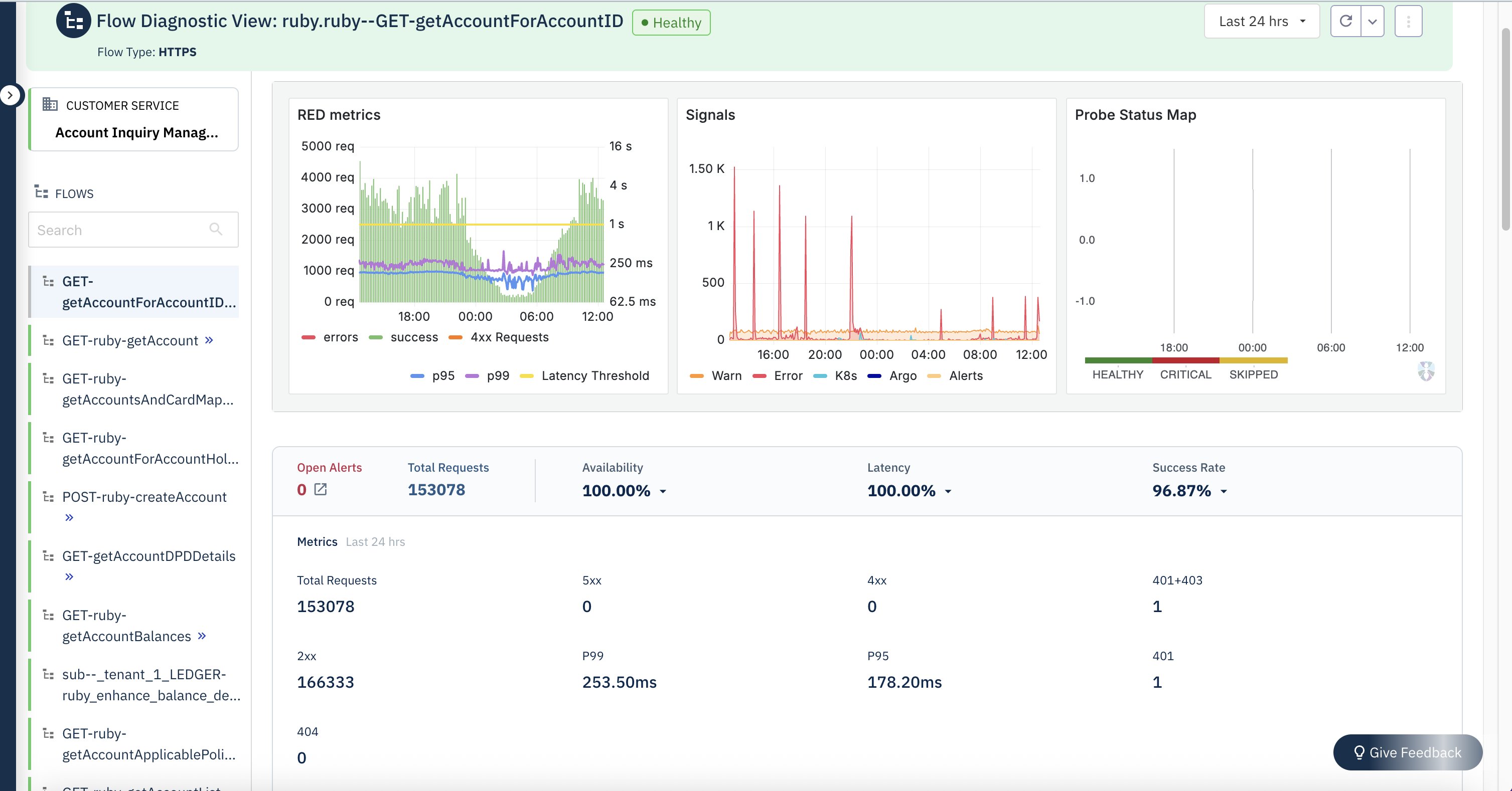
Turning back to what’s happening on October 15, 2025: We’re enabling Web Analytics so teams can track down performance bottlenecks. Web Analytics works by adding a lightweight JavaScript snippet to your website, which helps monitor performance metrics from visitors to your site. In the Web Analytics dashboard you can see aggregate performance data related to: how a browser has painted the page (via LCP, INP, and CLS), general load time metrics associated with server processing, as well as aggregate counts of visitors.

If you’ve ever popped open DevTools in your browser and stared at the waterfall chart of a slow-loading page, you’ve had a taste of what Web Analytics is doing, except instead of measuring your load times from your laptop, it’s measuring it directly from the browsers of real visitors.

Here’s the high-level architecture:

A lightweight beacon in the browser
Every page that you track with Cloudflare’s Web Analytics includes a tiny JavaScript snippet, optimized to load asynchronously so it won’t block rendering.

This snippet hooks into modern browser APIs like the Performance API, Resource Timing, etc
This is how Cloudflare collects Core Web Vital metrics like Largest Contentful Paint and Interaction to Next Paint, plus data about resource load times, TLS handshake duration from the perspective of the client.

Aggregation at the edge
When the browser sends performance data, it goes to the nearest Cloudflare data center. Instead of pushing raw events straight to a database, we pre-process at the edge. This reduces storage needs, minimizes latency, and removes personal information like IP addresses. After this pre-processing, it is sent to a core datacenter to be processed and queried by users.

Web Analytics sits under the Analytics & Logs section of the dashboard (at both the account and domain level of the dashboard). Starting on October 15, 2025, free domains will begin to see Web Analytics enabled by default and will be able to view the performance of their visitors in their dashboard. Pro, Biz and ENT accounts can enable Web Analytics by selecting the hostname of the website to add the snippet to and selecting Automatic Setup. Alternatively, you can manually paste the JavaScript beacon before the closing </body> tag on any HTML page you’d like to track from your origin. Just select “manage site” from the Web Analytics tab in the dashboard.

Once enabled, the JS snippet works with visitors’ browsers to measure how the user experienced page load times and reports on critical client-side metrics. Below these metrics are resource attribution tables that help users understand which assets are taking the most time per metrics to load so that users can better optimize their site performance.

What does privacy-first mean?

From the beginning, our Web Analytics tools have centered on providing insights without compromising privacy. Being privacy-first means we don’t track individual users for analytics. We don’t use any client-side state (like cookies or localStorage) for analytics purposes, and we don’t track users over time by IP address, User Agent, or any other fingerprinting technique.

Moreover, when enabling Web Analytics, you can choose to drop requests from European and UK visitors if you so desire (listed here specifically), meaning we will not collect any RUM metrics from traffic that passes through our European and UK data centers. The version of Web Analytics that will be enabled by default excludes data from EU visitors (this can be changed in the dashboard if you want).

The concept of a visit is key to our privacy approach. Rather than count unique IP addresses (requiring storing state about each visitor), we simply count page views that originate from a distinct referral or navigation event, avoiding the need to store information that might be considered personal data. We believe this same concept that we’ve used for years in providing our privacy-first Web Analytics can be logically extended to network and origin metrics. This will allow customers to gain the insights they need to debug and solve performance issues while ensuring they are not collecting unneeded data on visitors.

Opting-out

We built our Web Analytics service to give you the insights you need to run your website, all while maintaining a privacy-first approach. However, if you do want to opt-out, here are the steps to do so.

Via Dashboard

If you have a free domain and do not want Web Analytics automatically enabled for your zone you should do the following before October 15, 2025:

Navigate to the zone in the Cloudflare dashboard
In the list on the left of the screen, navigate to Web Analytics
On the next page, select either `Enable Globally` or `Exclude EU` to activate the feature
Once Web Analytics has been activated, navigate to `Manage RUM Settings` in the Web Analytics dashboard
Then, on the next page, select `Disable` to disable Web Analytics for the zone
OR, to remove Web Analytics from the zone entirely, delete the configs by clicking Advanced Options and then Delete

Once you have disabled the product once, we will not re-enable it again. You can choose to enable it whenever you want, however.

Via API

Create a Web Analytics configuration with the following API call:

curl https://api.cloudflare.com/client/v4/accounts/$ACCOUNT_ID/rum/site_info \
    -H 'Content-Type: application/json' \
    -H "X-Auth-Email: $CLOUDFLARE_EMAIL" \
    -H "X-Auth-Key: $CLOUDFLARE_API_KEY" \
    -d '{
          "auto_install": false,
          "host": "example.com",
          "zone_tag": "023e105f4ecef8ad9ca31a8372d0c353"
        }'

_{Note: This will not cause your zone to collect RUM data because auto_install is set to `false`}

Collect the site_tag and zone_tag fields from the response to this call
1. site_tag in this response will correspond to $SITE_ID in the following calls

EITHER Disable the Web Analytics configuration with the following API call:

curl https://api.cloudflare.com/client/v4/accounts/$ACCOUNT_ID/rum/site_info/$SITE_ID \
    -X PUT \
    -H 'Content-Type: application/json' \
    -H "X-Auth-Email: $CLOUDFLARE_EMAIL" \
    -H "X-Auth-Key: $CLOUDFLARE_API_KEY" \
    -d '{
          "auto_install": true,
          "enabled": false,
          "host": "example.com",
          "zone_tag": "023e105f4ecef8ad9ca31a8372d0c353"
        }'

OR Delete the Web Analytics configuration with the following API call:

curl https://api.cloudflare.com/client/v4/accounts/$ACCOUNT_ID/rum/site_info/$SITE_ID \
    -X DELETE \
    -H "X-Auth-Email: $CLOUDFLARE_EMAIL" \
    -H "X-Auth-Key: $CLOUDFLARE_API_KEY"

Where We’re Going Next

Today, Web Analytics gives you visibility into how people experience your site in the browser. Next, we’re expanding that lens to show what’s happening across the entire request path, from the click in a user’s browser, through Cloudflare’s global network, to your origin servers, and back.

Here’s what’s coming:

Correlating Across Layers
We’ll match RUM data from the client with network timing, Cloudflare edge processing, and origin response latency, allowing you to pinpoint whether a spike in TTFB comes from a slow script, a cache miss, or an origin bottleneck.
Proactive Alerting
Configurable alerts will tell you when performance regresses in specific geographies, when a data center underperforms, or when origin latency spikes.
Actionable Insights
We’ll go beyond “processing time” as a single number, breaking it into the real-world steps that make up the journey: proxy routing, security checks, cache lookups, origin fetches, and more.
Unified View
All of this will live in one place (your Cloudflare dashboard) alongside your analytics, logs, firewall events, and configuration settings, so you can see cause and effect in one workflow.

Conclusion

Stay tuned as we work alongside you, in public, to build the most comprehensive, privacy-focused performance analytics platform. Together, we will illuminate every corner of the request journey so you can optimize, innovate, and deliver the best experiences to your users, every time.

The next chapters of this journey will unlock proactive alerts, cross-layer correlation, and actionable insights you can’t get anywhere else. Follow along as the RUM Diaries are just getting started.

Automate and orchestrate Amazon EMR jobs using AWS Step Functions and Amazon EventBridge

2025-09-15 Senthil Kamala Rathinam

Post Syndicated from Senthil Kamala Rathinam original https://aws.amazon.com/blogs/big-data/automate-and-orchestrate-amazon-emr-jobs-using-aws-step-functions-and-amazon-eventbridge/

Many enterprises are adopting Apache Spark for scalable data processing tasks such as extract, transform, and load (ETL), batch analytics, and data enrichment. As data pipelines evolve, the need for flexible and cost-efficient execution environments that support automation, governance, and performance at scale also evolve in parallel. Amazon EMR provides a powerful environment to run Spark workloads, and depending on workload characteristics and compliance requirements, teams can choose between fully managed options like Amazon EMR Serverless or more customizable configurations using Amazon EMR on Amazon Elastic Compute Cloud (Amazon EC2).

In use cases where infrastructure control, data locality, or strict security postures are essential, such as in financial services, healthcare, or government, running transient EMR on EC2 clusters becomes a preferred choice. However, orchestrating the full lifecycle of these clusters, from provisioning to job submission and eventual teardown, can introduce operational overhead and risk if done manually.

To streamline this process, the AWS Cloud offers built-in orchestration capabilities using AWS Step Functions and Amazon EventBridge. Together, these services help you automate and schedule the entire EMR job lifecycle, reducing manual intervention while optimizing cost and compliance. Step Functions provides the workflow logic to manage cluster creation, Spark job execution, and cluster termination, and EventBridge schedules these workflows based on business or operational needs.

In this post, we discuss how to build a fully automated, scheduled Spark processing pipeline using Amazon EMR on EC2, orchestrated with Step Functions and triggered by EventBridge. We walk through how to deploy this solution using AWS CloudFormation, processes COVID-19 public dataset data in Amazon Simple Storage Service (Amazon S3), and store the aggregated results in Amazon S3. This architecture is ideal for periodic or scheduled batch processing scenarios where infrastructure control, auditability, and cost-efficiency are critical.

Solution overview

This solution uses the publicly available COVID-19 dataset to illustrate how to build a modular, scheduled architecture for scalable and cost-efficient batch processing for time-bound data workloads.The solution follows these steps:

Raw COVID-19 data in CSV format is stored in an S3 input bucket.
A scheduled rule in EventBridge triggers a Step Functions workflow.
The Step Functions workflow provisions a transient Amazon EMR cluster using EC2 instances.
A PySpark job is submitted to the cluster to calculate COVID-19 hospital utilization data to compute monthly state-level averages of inpatient and ICU bed utilization, and COVID-19 patient percentages.
The processed results are written back to an S3 output bucket.
After successful job completion, the EMR cluster is automatically deleted.
Logs are persisted to Amazon S3 for observability and troubleshooting.

By automating this workflow, you alleviate the need to manually manage EMR clusters while gaining cost-efficiency by running compute only when needed. This architecture is ideal for periodic Spark jobs such as ETL pipelines, regulatory reporting, and batch analytics, especially when control, compliance, and customization are required.The following diagram illustrates the architecture for this use case.

The infrastructure is deployed using AWS CloudFormation to provide consistency and repeatability. AWS Identity and Access Management (IAM) roles grant least‑privilege access to Step Functions, Amazon EMR, EC2 instances, and S3 buckets, and optional AWS Key Management Service (AWS KMS) encryption can secure data at rest in Amazon S3 and Amazon CloudWatch Logs. By combining a scheduled trigger, stateful orchestration, and centralized logging, this solution delivers a fully automated, cost‑optimized, and secure way to run transient Spark workloads in production.

Prerequisites

Before you get started, make sure you have the following prerequisites:

An AWS account. If you don’t have one, you can sign up for one.
An IAM user with administrator access. For instructions, see Create a user with administrative access.
The AWS Command Line Interface (AWS CLI) is installed on your local machine
A default virtual private cloud (VPC) and subnet in the target AWS Region where you plan to run the CloudFormation template.

Set up resources with AWS CloudFormation

To provision the required resources using a single CloudFormation template, complete the following steps:

Clone the sample repository to your local machine or AWS CloudShell and navigate into the project directory.

git clone https://github.com/aws-samples/sample-emr-transient-cluster-step-functions-eventbridge.git
cd sample-emr-transient-cluster-step-functions-eventbridge

Set an environment variable for the AWS Region where you plan to deploy the resources. Replace the placeholder with your Region code, for example, us-east-1.
```
export AWS_REGION=<YOUR AWS REGION>
```

Deploy the stack using the following command. Update the stack name if needed. In this example, the stack is created with the name covid19-analysis.

aws cloudformation deploy \
--template-file emr_transient_cluster_step_functions_eventbridge.yaml \
--stack-name covid19-analysis \
--capabilities CAPABILITY_IAM \
--region $AWS_REGION

You can monitor the stack creation progress on the AWS CloudFormation console on the Events tab. The deployment typically completes in under 5 minutes.

After the stack is successfully created, go to the Outputs tab on the AWS CloudFormation console and note the following values for use in later steps:

InputBucketName
OutputBucketName
LogBucketName

Set up the COVID-19 dataset

With your infrastructure in place, complete the following steps to set up the input data:

Download the COVID-19 data CSV file from HealthData.gov to your local machine.
Rename the downloaded file to covid19-dataset.csv.
Upload the renamed file to your S3 input bucket under the raw/ folder path.

Set up the PySpark Script

Complete the following steps to set up the PySpark script:

Open AWS CloudShell from the console.
Confirm that you are working inside the sample-emr-transient-cluster-step-functions-eventbridge directory before running the next command.
Copy the PySpark script needed for this walkthrough into your input bucket:
```
aws s3 cp covid19_processor.py s3://<InputBucketName>/scripts/
```

This script processes COVID-19 hospital utilization data stored as CSV files in your S3 input bucket. When running the job, provide the following command-line arguments:

--input – The S3 path to the input CSV files
--output – The S3 path to store the processed results

The script reads the raw dataset, standardizes various date formats, and filters out records with invalid or missing dates. It then extracts key utilization metrics such as inpatient bed usage, ICU bed usage, and the percentage of beds occupied by COVID-19 patients and calculates monthly averages grouped by state. The aggregated output is saved as timestamped CSV files in the specified S3 location.

This example demonstrates how you can use PySpark to efficiently clean, transform, and analyze large-scale healthcare data to gain actionable insights on hospital capacity trends during the pandemic.

Configure a schedule in EventBridge

The Step Functions state machine is by default scheduled to run on December 31, 2025, as a one-time execution. You can update the schedule for recurring or one-time execution as needed. Complete the following steps:

On the EventBridge console, choose Schedules under Scheduler in the navigation pane.
Select the schedule named <StackName>-covid19-analysis and choose Edit.
Set your preferred schedule pattern.
1. If you want to run the schedule one time, select One-time schedule for Occurrence and enter a date and time.
2. If you want to run this on a recurring basis, select Recurring schedule. Specify the schedule type as either Cron-based schedule or Rate-based schedule as needed.
Choose Next twice and choose Save schedule.

Start the workflow in Step Functions

Based on your EventBridge schedule, the Step Functions workflow will run automatically. For this walkthrough, complete the following steps to trigger it manually:

On the Step Functions console, choose State machines in the navigation pane.
Choose the state machine that begins with Covid19AnalysisStateMachine-*.
Choose Start execution.
In the Input section, provide the following JSON (provide the log bucket and output bucket names with the appropriate values captured earlier):
```
{
  "LogUri": "s3://<LogBucketName>/logs/",
  "OutputS3Location": "s3://<OutputBucketName>/processed/"
}
```
Choose Start execution to initiate the workflow.

Monitor the EMR job and workflow execution

After you start the workflow, you can track both the Step Functions state transitions and the EMR job progress in real time on the console.

Monitor the Step Functions state machine

Complete the following steps to monitor the Step Functions state machine:

On the Step Functions console, choose State machines in the navigation pane.
Choose the state machine that begins with Covid19AnalysisStateMachine-*.
Choose the running execution to view the visual workflow.
Each state node will update as it progresses—green for success, red for failure.
To explore a step, choose its node and inspect the input, output, and error details in the side pane.

The following screenshot shows an example of a successfully executed workflow.

Monitor the EMR cluster and EMR step

Complete the following steps to monitor the EMR cluster and EMR step status:

While the cluster is active, open the Amazon EMR console and choose Clusters in the navigation pane.
Locate the Covid19Cluster transient EMR cluster.
Initially, it will be in Starting status.

On the Steps tab, you can see your Spark submit step listed. As the job progresses, the step status changes from Pending to Running to finally Completed or Failed.
Choose the Applications tab to view the application UIs, in which you can access the Spark History Server and YARN Timeline Server for monitoring and troubleshooting.

Monitor CloudWatch logs

To enable CloudWatch logging and enhanced monitoring for your EMR on EC2 cluster, refer to Amazon EMR on EC2 – Enhanced Monitoring with CloudWatch using custom metrics and logs. This guide explains how to install and configure the CloudWatch agent using a bootstrap action, so you can stream system-level metrics (such as CPU, memory, and disk usage) and application logs from EMR nodes directly to CloudWatch. With this setup, you can gain real-time visibility into cluster health and performance, simplify troubleshooting, and retain critical logs even after the cluster is terminated.

For this walkthrough, check the logs in the S3 log output location.

Confirm cluster deletion

When the Spark step is complete, Step Functions will automatically delete the Amazon EMR cluster. Refresh the Clusters page on the Amazon EMR console. You should see your cluster status change from Terminating to Terminated within a minute.

By following these steps, you gain full end-to-end visibility into your workflow from the moment the Step Functions state machine is triggered to the automatic shutdown of the EMR cluster. You can monitor execution progress, troubleshoot issues, confirm job success, and continuously optimize your transient Spark workloads.

Verify job output in Amazon S3

When the job is complete, complete the following steps to check the processed results in the S3 output bucket:

On the Amazon S3 console, choose Buckets in the navigation pane.
Open the output S3 bucket you noted earlier.
Open the processed folder.
Navigate into the timestamped subfolder to view the CSV output file.
Download the CSV file to view the processed results, as shown in the following screenshot.

Monitoring and troubleshooting

To monitor the progress of your Spark job running on a transient EMR on EC2 cluster, use the Step Functions console. It provides real-time visibility into each state transition in your workflow, from cluster creation and job submission to cluster deletion. This makes it straightforward to track execution flow and identify where issues might occur.During job execution, you can use the Amazon EMR console to access cluster-level monitoring. This includes YARN application statuses, step-level logs, and overall cluster health. If CloudWatch logging is enabled in your job configuration, driver and executor logs stream in near real time, so you can quickly detect and diagnose errors, resource constraints, or data skew within your Spark application.

After the workflow is complete, regardless of whether it succeeds or fails, you can perform a detailed post-execution analysis by reviewing the logs stored in the S3 bucket specified in the LogUri parameter. This log directory includes standard output and error logs, along with Spark history files, offering insights into execution behavior and performance metrics.

For continued access to the Spark UI during job execution, you can use persistent application UIs on the EMR console. These links remain accessible even after the cluster is stopped, enabling deeper root-cause analysis and performance tuning for future runs.

This visibility into both workflow orchestration and job execution can help teams optimize their Spark workloads, reduce troubleshooting time, and build confidence in their EMR automation pipelines.

Clean up

To avoid incurring ongoing charges, clean up the resources provisioned during this walkthrough:

Empty the S3 buckets:
1. On the Amazon S3 console, choose Buckets in the navigation pane.
2. Select the input, output, and log buckets used in this tutorial.
3. Choose Empty to remove all objects before deleting the buckets (optional).
Delete the CloudFormation stack:
1. On the AWS CloudFormation console, choose Stacks in the navigation pane.
2. Select the stack you created for this solution and choose Delete.
3. Confirm the deletion to remove associated resources.

Conclusion

In this post, we showed how to build a fully automated and cost-effective Spark processing pipeline using Step Functions, EventBridge, and Amazon EMR on EC2. The workflow provisions a transient EMR cluster, runs a Spark job to process data, and stops the cluster after the job completes. This approach helps reduce costs while giving you full control over the process. This solution is ideal for scheduled data processing tasks such as ETL jobs, log analytics, or batch reporting, especially when you need detailed control over infrastructure, security, and compliance settings.

To get started, deploy the solution in your environment using the CloudFormation stack provided and adjust it to fit your data processing needs. Check out the Step Functions Developer Guide and Amazon EMR Management Guide to explore further.

Share your feedback and ideas in the comments or connect with your AWS Solutions Architect to fine-tune this pattern for your use case.

About the authors

Streamline Spark application development on Amazon EMR with the Data Solutions Framework on AWS

2025-09-15 Vincent Gromakowski

Post Syndicated from Vincent Gromakowski original https://aws.amazon.com/blogs/big-data/streamline-spark-application-development-on-amazon-emr-with-the-data-solutions-framework-on-aws/

Today, organizations are heavily using Apache Spark for their big data processing needs. However, managing the entire development lifecycle of Spark applications—from local development to production deployment—can be complex and time-consuming. Managing the entire code base—including application code, infrastructure provisioning, and continuous integration and delivery (CI/CD) pipelines—is sometimes not fully automated and a shared responsibility across multiple teams, which slows down release cycles. This undifferentiated heavy lifting diverts valuable resources away from core business objectives: deriving value from data.

In this post, we explore how to use Amazon EMR, the AWS Cloud Development Kit (AWS CDK), and the Data Solutions Framework (DSF) on AWS to streamline the development process, from setting up a local development environment to deploying serverless Spark infrastructure, and implementing a CI/CD pipeline for automated testing and deployment.

By adopting this approach, developers gain full control over their code and the infrastructure responsible for running it, alleviating the need for cross-team dependency. Developers can customize the infrastructure to meet specific business needs and optimize performance. Additionally, they can customize CI/CD stages to facilitate comprehensive testing, using the self-mutation capability of AWS CDK Pipelines to automatically update and refine the deployment process. This level of control not only accelerates development cycles but also enhances the reliability and efficiency of the entire application lifecycle, so developers can focus more on innovation and less on manual infrastructure management.

Solution overview

The solution consists of the following key components:

The local development environment to develop and test your Spark code locally
The infrastructure as code (IaC) that will run your Spark application in AWS environments
The CI/CD pipeline running end-to-end tests and deploying into the different AWS environments

In the following sections, we discuss how to set up these components.

Prerequisites

To set up this solution, you must have an AWS account with appropriate permissions, Docker and the AWS CDK CLI.

Set up the local development environment

Developing Spark applications locally can be a challenging task due to the need for a consistent and efficient environment that mirrors your production setup. With Amazon EMR, Docker, and the Amazon EMR toolkit extension for Visual Studio Code, you can quickly set up a local development environment for Spark applications, developing and testing Spark code locally, and seamlessly port it to the cloud.

The Amazon EMR toolkit for VS Code includes an “EMR: Create Local Spark Environment” command that generates a development container. This container is based on an Amazon EMR on Amazon EKS image corresponding to the Amazon EMR version you select. You can develop Spark and PySpark code locally, with full compatibility with your remote Amazon EMR environment. Additionally, the toolkit provides helpers to make it straightforward to connect to the AWS Cloud, including an Amazon EMR explorer, an AWS Glue Data Catalog explorer, and commands to run Amazon EMR Serverless jobs from VS Code.

To set up your local environment, complete the following steps:

Install VS Code and the Amazon EMR Toolkit for VS Code.
Install and launch Docker.
Create a local Amazon EMR environment in your working directory using the command EMR: Create Local Spark Environment.

Amazon EMR Toolkit bootstrap

Choose PySpark, Amazon EMR 7.5, and the AWS Region you want to use, and choose an authentication mechanism.

Amazon EMR toolkit local environment

aws ecr get-login-password --region us-east-1 \
    | docker login \
    --username AWS \
    --password-stdin \
    12345678910.dkr.ecr.us-east-1.amazonaws.com

Now you can launch your dev container using the VS Code command Dev Containers: Rebuild and Reopen in container.

The container will install the latest operating system packages and run a local Spark history server on port 18080.

local Spark history server

The container provides spark-shell, spark-sql, and pyspark from the terminal and a Jupyter Python kernel for connecting a Jupyter notebook to execute interactive Spark code.

local Jupyter notebooks

Using the Amazon EMR Toolkit, you can develop your Spark application and test it locally using Pytest—for example, to validate the business logic. You can also connect to other AWS accounts where you have your development environment.

Build the AWS CDK application with DSF on AWS

After you validate the business logic into your local Spark application, you can implement the infrastructure responsible for running your application. DSF provides AWS CDK L3 Constructs that simplify the creation of Spark-based data pipelines on EMR Serverless or Amazon EMR on EKS.

DSF provides the capability to package your local PySpark application, including the Python dependencies, into artifacts that can consumed by EMR Serverless jobs. The PySparkApplicationPackage is a construct that uses a Dockerfile to perform the packaging of dependencies into a Python virtual environment archive and then upload the archive and the PySpark entrypoint file into a secured Amazon Simple Storage Service (Amazon S3) bucket. The following diagram illustrates this architecture.

PySparkApplicationPackage L3 construct

See the following example code:

spark_app = dsf.processing.PySparkApplicationPackage(
    self,
    "SparkApp",
    entrypoint_path="./../spark/src/agg_trip_distance.py",
    application_name="TaxiAggregation",
    # Path of the Dockerfile used to package the dependencies as a Python venv
    dependencies_folder='./../spark',
    # Path of the venv archive in the docker image
    venv_archive_path="/venv-package/pyspark-env.tar.gz",
    removal_policy=RemovalPolicy.DESTROY)

You just need to provide the paths for the following:

The PySpark entrypoint. This is the main Python script of your Spark application.
The Dockerfile containing the logic for packaging a virtual environment into an archive.
The path of the resulting archive in the container file system.

DSF provides helpers to connect the application package to the EMR Serverless job. The PySparkApplicationPackage construct exposes properties that can directly be used into the SparkEmrServerlessJob construct parameters. This construct simplifies the configuration of a batch job using an AWS Step Functions state machine. The following diagram illustrates this architecture.

EmrServerlessJob L3 construct

The following code is an example of an EMR Serverless job:

spark_job = dsf.processing.SparkEmrServerlessJob(
    self,
    "SparkProcessingJob",
    dsf.processing.SparkEmrServerlessJobProps(
        name=f"taxi-agg-job-{Names.unique_resource_name(self)}",
        # ID of the previously created EMR Serverless runtime
        application_id=spark_runtime.application.attr_application_id,
        # The IAM role used by the EMR Job with permissions required by the application
        execution_role=processing_exec_role,
        spark_submit_entry_point=spark_app.entrypoint_uri,
        # Add the Spark parameters from the PySpark package to configure the dependencies (using venv)
        spark_submit_parameters=spark_app.spark_venv_conf + spark_params,
        removal_policy=RemovalPolicy.DESTROY,
        schedule=schedule))

Note the two parameters of SparkEmrServerlessJob that are provided by PySparkApplicationPackage:

entrypoint_uri, which is the S3 URI of the entrypoint file
spark_venv_conf, which contains the Spark submit parameters for using the Python virtual environment

DSF also provides a SparkEmrServerlessRuntime to simplify the creation of the EMR Serverless application responsible for running the job.

Deploy the Spark application using CI/CD

The final step is to implement a CI/CD pipeline that can test your Spark code and promote from dev/test/stage and then to production. DSF provides a L3 Construct that simplifies the creation of the CI/CD pipeline for your Spark applications. DSF’s implementation of the Spark CI/CD pipeline construct uses the AWS CDK built-in pipeline functionality. One of the key capabilities when using an AWS CDK pipeline is its self-mutating capability. It can update itself whenever you change its definition, avoiding the traditional chicken-and-egg problem of pipeline updates and helping developers fully control their CI/CD pipeline.

When the pipeline runs, it follows a carefully orchestrated sequence. First, it retrieves your code from your repository and synthesizes it into AWS CloudFormation templates. Before doing anything else, it examines these templates to see if you’ve made any changes to the pipeline’s own structure. If the pipeline detects that its definition has changed, it will pause its normal operation and update itself first. After the pipeline has updated itself, it will continue with its regular stages, such as deploying your application.

DSF provides an opinionated implementation of CDK Pipelines for Spark applications, where the PySpark code is automatically unit tested using Pytest and where the configuration is simplified. You only need to configure four components:

The CI/CD stages (testing, staging, production, and so on). This includes the AWS account ID and Region where these environments reside in.
The AWS CDK stack that is deployed in each environment.
(Optional) The integration test script that you want to run against the deployed stack.
The SparkEmrCICDPipeline AWS CDK construct.

The following diagram illustrates how everything works together.

SparkCICDPipeline L3 construct

Let’s dive into each of these components.

Define cross-account deployment and CI/CD stages

With the SparkEmrCICDPipeline construct, you can deploy your Spark application stack across different AWS accounts. For example, you can have a separate account for your CI/CD processes and different accounts for your staging and production environments.To set this up, first bootstrap the various AWS accounts (staging, production, and so on):

cdk bootstrap --profile <ENVIRONMENT_ACCOUNT_PROFILE> \ 
    aws://<ENVIRONMENT_ACCOUNT_ID&gt;/&lt;REGION> \ 
    --trust <CICD_ACCOUNT_ID> \ 
    --cloudformation-execution-policies "POLICY_ARN"

This step sets up the necessary resources in the environment accounts and creates a trust relationship between those accounts and the CI/CD account where the pipeline will run.Next, choose between two options to define the environments (both options require the relevant configuration in the cdk.context.json file.The first option is to use pre-defined environments, which is defined as follows:

{ 
    "staging": { 
        "account": "<STAGING_ACCOUNT_ID>", 
        "region": "<REGION>" 
    }, 
    "prod": { 
        "account": "<PROD_ACCOUNT_ID>", 
        "region": "<REGION>" 
    } 
}

Alternatively, you can use user-defined environments, which is defined as follows:

{
   "environments":[
      {
         "stageName":"<STAGE_NAME_1>",
         "account":"<STAGE_ACCOUNT_ID>",
         "region":"<REGION>",
         "triggerIntegTest":"<OPTIONAL_BOOLEAN_CAN_BE_OMMITTED>"
      },
      {
         "stageName":"<STAGE_NAME_2>",
         "account":"<STAGE_ACCOUNT_ID>",
         "region":"<REGION>",
         "triggerIntegTest":"<OPTIONAL_BOOLEAN_CAN_BE_OMMITTED>"
      },
      {
         "stageName":"<STAGE_NAME_3>",
         "account":"<STAGE_ACCOUNT_ID>",
         "region":"<REGION>",
         "triggerIntegTest":"<OPTIONAL_BOOLEAN_CAN_BE_OMMITTED>"
      }
   ]
}

Customize the stack to be deployed

Now that the environments have been bootstrapped and configured, let’s look at the actual stack that contains the resources that will be deployed in the various environments. Two classes must be implemented:

A class that extends the stack – This is where the resources that are going to be deployed in each of the environments are defined. This can be a normal AWS CDK stack, but it can be deployed in another AWS account depending on the environment configuration defined in the previous section.
A class that extends ApplicationStackFactory – This is DSF specific, and makes it possible to configure and then return the stack that is created.

The following code shows a full example:

class MyApplicationStack(cdk.Stack): 
    def __init__(self, scope, *, stage): 
        super().__init__(scope, "MyApplicationStack") 
        bucket = Bucket(self, "TestBucket",
                        auto_delete_objects=True, 
                        removal_policy=cdk.RemovalPolicy.DESTROY) 
        cdk.CfnOutput(self, "BucketName", value=bucket.bucket_name) 
        
class MyStackFactory(dsf.utils.ApplicationStackFactory): 
    def create_stack(self, scope, stage): 
        return MyApplicationStack(scope, stage=stage)

ApplicationStackFactory supports customization of the stack before returning the initialized object to be deployed by the CI/CD pipeline. You can customize your stack behavior by passing the current stage to your stack. For example, you can skip scheduling the Spark application in the integration tests stage because the integration tests trigger it manually as part of the CI/CD pipeline. For the production stage, the scheduling facilitates automatic execution of the Spark application.

Write the integration test script

The integration test script is a bash script that is triggered after the main application stack has been deployed. Inputs to the bash script can come from the AWS CloudFormation outputs of the main application stack. These outputs are mapped into environment variables that the bash script can access directly.

In the Spark CI/CD example, the application stack uses the SparkEMRServerlessJob CDK construct. This construct uses a Step Functions state machine to manage the execution and monitoring of the Spark job. The following is an example integration test bash script that we use to test that the deployed stack can run the associated Spark job successfully:

#!/bin/bash 
EXECUTION_ARN=$(aws stepfunctions start-execution --state-machine-arn $STEP_FUNCTION_ARN | jq -r '.executionArn')

while true 
do 
    STATUS=$(aws stepfunctions describe-execution --execution-arn $EXECUTION_ARN | jq -r '.status') 
    if [ $STATUS = "SUCCEEDED" ]; then 
        exit 0 
    elif [ $STATUS = "FAILED" ] || [ $STATUS = "TIMED_OUT" ] || [ $STATUS = "ABORTED" ]; then 
        exit 1 
    else 
        sleep 10
        continue 
    fi
done

The integration test scripts are executed within an AWS CodeBuild project. As part of the IntegrationTestStack, we’ve included a custom resource that periodically checks the status of the integration test script as it runs. Failure of the CodeBuild execution causes the parent pipeline (residing in the pipeline account) to fail. This helps teams only promote changes that pass all the required testing.

Bring all the components together

When you have your components ready, you can use the SparkEmrCICDPipeline to bring them together. See the following example code:

dsf.processing.SparkEmrCICDPipeline(
    self,
    "SparkCICDPipeline",
    spark_application_name="SparkTest",
    # The Spark image to use in the CICD unit tests
    spark_image=dsf.processing.SparkImage.EMR_7_5,
    # The factory class to dynamically pass the Application Stack
    application_stack_factory=SparkApplicationStackFactory(),
    # Path of the CDK python application to be used by the CICD build and deploy phases
    cdk_application_path="infra",
    # Path of the Spark application to be built and unit tested in the CICD
    spark_application_path="spark",
    # Path of the bash script responsible to run integration tests 
    integ_test_script='./infra/resources/integ-test.sh',
    # Environment variables used by the integration test script, value is the CFN output name
    integ_test_env={
        "STEP_FUNCTION_ARN": "ProcessingStateMachineArn"
    },
    # Additional permissions to give to the CICD to run the integration tests
    integ_test_permissions=[
        PolicyStatement(
            actions=["states:StartExecution", "states:DescribeExecution"
            ],
            resources=["*"]
        )
    ],
    source= CodePipelineSource.connection("your/repo", "branch",
        connection_arn="arn:aws:codeconnections:us-east-1:222222222222:connection/7d2469ff-514a-4e4f-9003-5ca4a43cdc41"
    ),
    removal_policy=RemovalPolicy.DESTROY,
)

The following elements of the code are worth highlighting:

With the integ_test_env parameter, you can define the environment variable mapping with the output of your application stack that’s defined in the application_stack_factory parameter
The integ_test_permissions parameter specifies the AWS Identity and Access Management (IAM) permissions that are attached to the CodeBuild project where the integration test script runs in
CDK Pipelines needs an AWS code connection Amazon Resource Name (ARN) to connect to your Git repository when you host your code

Now you can deploy the stack containing the CI/CD pipeline. This is a one-time operation because the CI/CD pipeline will dynamically be updated based on code changes that impact the CI/CD pipeline itself:

cd infra 
cdk deploy CICDPipeline

Then you can commit and push the code into the source code repository defined in the source parameter. This step triggers the pipeline and deploys the application in the configured environments. You can check the pipeline definition and status on the AWS CodePipeline console.

AWS CodePipeline

You can find the full example on the Data Solutions Framework GitHub repository.

Clean up

Follow the readme guide to delete the resources created by the solution.

Conclusion

By using Amazon EMR, the AWS CDK, DSF on AWS, and the Amazon EMR toolkit, developers can now streamline their Spark application development process. The solution described in this post helps developers gain full control over their code and infrastructure, making it possible to set up local development environments, implement automated CI/CD pipelines, and deploy serverless Spark infrastructure across multiple environments.

DSF supports other patterns, such as streaming governance and data sharing and Amazon Redshift data warehousing. The DSF roadmap is publicly available, and we look forward to your feature requests, contributions, and feedback. You can get started using DSF by following our Quick start guide.

About the authors

Use the Amazon DataZone upgrade domain to Amazon SageMaker and expand to new SQL analytics, data processing, and AI uses cases

2025-09-11 David Victoria

Post Syndicated from David Victoria original https://aws.amazon.com/blogs/big-data/use-the-amazon-datazone-upgrade-domain-to-amazon-sagemaker-and-expand-to-new-sql-analytics-data-processing-and-ai-uses-cases/

Amazon DataZone and Amazon SageMaker announced a new feature that allows an Amazon DataZone domain to be upgraded to the next generation of SageMaker, making the investment customers put into developing Amazon DataZone transferable to SageMaker. All content created and curated through Amazon DataZone such as assets, metadata forms, glossaries, subscriptions, and so on are available to users through Amazon SageMaker Unified Studio after the upgrade.

As an Amazon DataZone administrator, you can choose which of your domains to upgrade to SageMaker through a user interface driven experience. You can use the upgraded domain to use your existing Amazon DataZone implementation in the new SageMaker environment and expand to new SQL analytics, data processing and AI uses cases. Additionally, after the upgrade, both Amazon DataZone and SageMaker portals remain accessible. This provides administrators flexibility with user rollout of SageMaker while providing business continuity for users operating within Amazon DataZone. By upgrading to SageMaker, users can build on their investment from Amazon DataZone by using the SageMaker unified platform, which serves as a central hub for all data, analytics, and AI needs.

SageMaker delivers an integrated experience for analytics and AI with unified access to all your data. Collaborate and build faster from a unified studio using familiar Amazon Web Services (AWS) tools for model development, generative AI, data processing, and SQL analytics, accelerated by Amazon Q Developer, the most capable generative AI assistant for software development. Access all your data whether it’s stored in data lakes, data warehouses, or third-party or federated data sources, with governance built in to meet enterprise security needs.

What we hear from customers

Customers have successfully used Amazon DataZone, enabling data analysts, data engineers, and machine learning teams to collaborate around a shared data catalog. With generative AI moving to center stage, these organizations now aim to address a wider range of use cases, from interactive notebook exploration to prompt engineering for generative-AI projects. Upgrading their Amazon DataZone domains to SageMaker Unified Studio brings everyone together in one place. Data analysts, data engineers, machine learning (ML) specialists, and AI innovators can create integrated solutions on the same governed data while using the tools that best match their work. For example, one of our customers, HEMA, uses Amazon DataZone as a single solution for cataloging, discovery, sharing, and governance of their enterprise data across business domains. They are moving to SageMaker to enable more machine learning and generative AI use cases.

“The launch of the domain upgrade feature allows us to take the investment from our production Amazon DataZone deployment and utilize it in Amazon SageMaker. Organizationally, we are doing more in the generative AI space and with Amazon SageMaker we can accomplish new use cases that leverage the assets curated through Amazon DataZone. With this feature we also love that both portals remain open at the same time so that we can thoughtfully transition user populations to Amazon SageMaker.”

– Tommaso Paracciani, Head of Data & Cloud Platforms at HEMA.

“We’ve invested a lot in building our data management platform for production and logistics, using Amazon DataZone, to accelerate our digital transformation. Evolving our data management solution to use Amazon SageMaker Unified Studio means Data Analysis, Data Engineering, Machine Learning & Generative AI features can now be done from the same place. With the domain upgrade feature, it allows us to onboard to Amazon SageMaker faster by utilizing the work done from Amazon DataZone“

– Volkswagen AG

Upgrade your Amazon DataZone domain to SageMaker Unified Studio

On your Amazon DataZone domain home page, a banner appears at the top announcing the new domain upgrade feature. Choose Get started on this banner to open the upgrade wizard.

A summary page explains the actions the upgrade wizard will perform and what to expect while it runs. Read the information carefully, then choose Start to begin the upgrade.

On the configuration screen, specify the AWS Identity and Access Management (IAM) roles and ownership for your new SageMaker Unified Studio domain:
1. Domain execution role – The runtime role the domain assumes for SageMaker operations.
2. Domain service role – Authorizes the service to create and manage domain resources.
3. Root domain owner (optional) – Designates the administrators of the upgraded root domain. IAM roles cannot sign in to the SageMaker Unified Studio UI. It is helpful to have a root domain owner who can sign in to the UI to modify authorization policies for the root domain.

After selecting the appropriate roles—and, if applicable, a root owner—choose Upgrade domain to launch the upgrade.

When the upgrade finishes, a confirmation banner appears at the top of the domain detail page with two items:
1. The Amazon DataZone portal URL
2. The Manage Amazon DataZone upgrade button. Here you can see the Amazon DataZone URL, information about the upgrade, and an option to roll back the upgrade to Amazon DataZone.

Scroll to the Users section of the SageMaker Unified Studio console. All identities that belonged to your original Amazon DataZone domain—along with the root domain owner you assigned in Step 3—now appear in the new domain automatically. No additional setup is required.

Use the URL provided in Step 4 to open SageMaker Unified Studio, then sign in with your existing credentials. You’ll land on the SageMaker Unified Studio home page, confirming that you’re now working in your upgraded domain.

In the Projects list, choose a project that existed in your original Amazon DataZone domain and that the current user can access. Select its name to open it and confirm that every asset and permission transferred correctly to SageMaker Unified Studio.

Inside the project, you can view two key areas:
- Project Environments – Verify that every environment linked to the project has been migrated.
- Overview – Confirm the project’s general information, including owner, description, and status.

Checking both sections helps ensure that the project moved to SageMaker Unified Studio as expected.

Conclusion

In this post, we discussed the new capability in Amazon DataZone that allows a domain to be upgraded to the next generation of Amazon SageMaker. The investment customers put into developing Amazon DataZone is now transferable to SageMaker. All content created and curated through Amazon DataZone such as assets, metadata forms, glossaries, subscriptions, and so on are available to users through SageMaker Unified Studio after the upgrade. By upgrading to SageMaker, customers build on their investment from Amazon DataZone by using the SageMaker unified platform.

To learn more, visit the domain upgrade documentation.

About the authors

David Victoria is a Senior Technical Product Manager with Amazon SageMaker at AWS. He focuses on improving administration and governance capabilities needed for customers to support their analytics systems. He is passionate about helping customers realize the most value from their data in a secure, governed manner.

Leonardo David Gomez Virahonda is a Principal Analytics Specialist Solutions Architect at AWS, with a strong focus on data governance. He helps organizations across industries implement effective governance strategies using AWS services like Amazon DataZone, AWS Glue, Lake Formation, and SageMaker Catalog. Leonardo’s work spans metadata management, data lineage, access control, and compliance—empowering customers to make their data secure, discoverable, and ready for analytics and AI. He regularly shares best practices through technical blogs, enablement content, and sessions at AWS events like re:Invent and regional Summits.

Introducing restricted classification terms for governed classification in Amazon SageMaker Catalog

2025-09-08 Ramesh H Singh

Post Syndicated from Ramesh H Singh original https://aws.amazon.com/blogs/big-data/introducing-restricted-classification-terms-for-governed-classification-in-amazon-sagemaker-catalog/

Security and compliance concerns are key considerations when customers across industries rely on Amazon SageMaker Catalog. Customers use SageMaker Catalog to organize, discover, and govern data and machine learning (ML) assets. A common request from domain administrators is the ability to enforce governance controls on certain metadata terms that carry compliance or policy significance. Examples include terms used to classify assets with sensitive data (such as PHI in healthcare or PCI in financial services) or terms used to trigger automatic access grants based on regulatory or organizational policies.

AWS announced restricted classification terms in SageMaker Catalog. This new capability allows domain administrators to define governance-controlled terms and enforce which teams and users are authorized to apply them. Restricted classification terms are designed to allow organizations to set standards for consistent classification of sensitive data, help prevent misuse of regulatory tags, and enable downstream workflows such as automatic access grants across the enterprise.

Restricted classification (glossary) terms

Customers have told us that the flexibility of applying glossary terms in SageMaker Catalog has been valuable for collaboration and scale. At the same time, many enterprises—especially in regulated industries—wanted an additional layer of control for certain classifications. For example, terms like PHI (Protected Health Information) in healthcare or PCI (payment card industry) in financial services should only be applied by authorized personnel, because they carry compliance and policy significance. Customers also asked for a way to enforce these governance policies without adding operational overhead. As catalogs grow to thousands of assets, forms, and columns, validating tens of thousands of terms can create performance and compliance challenges. A solution was needed to combine the openness of cataloging with governance precision for sensitive use cases.With this launch, SageMaker Catalog introduces a restricted classification terms section on each asset:

Business glossary terms (existing): Open tagging, no restrictions.
Restricted glossary terms (new): Only authorized users or groups can apply terms. Unauthorized users can view and filter assets based on these terms but not assign them.

Customer spotlight

As a large-scale organization with diverse data needs, the Business Data Technologies (BDT) team at Amazon manages thousands of assets across business units. Making sure these assets are consistently classified and governed is critical to maintaining compliance and enabling secure data sharing at scale. With restricted classification terms in SageMaker Catalog, the BDT team can now enforce which groups are authorized to apply terms, such as policy-driven classifications for merchants or payment data, while keeping discovery seamless for users.

“Restricted classification terms are instrumental in helping us scale data onboarding and governance across Amazon. By enforcing who can apply policy-related terms in the Amazon SageMaker Catalog, we’re able to accelerate consolidation of data assets across business units without compromising compliance. This facilitates consistent classification, prevents misuse, and allows us to automate downstream access grants—enabling our builders to innovate quickly while maintaining the highest standards of governance.”

– Gerry Moses, Senior Principal Technologist, Business Data Technologies, Amazon

Key benefits

With the introduction of restricted classification terms, customers gain stronger governance controls without losing the flexibility of open cataloging. This capability is designed to provide customers with the following key benefits:

Governance enforcement – Sensitive terms such as PHI or PCI can only be applied by approved users or groups, supporting compliance with organizational and regulatory policies.
Consistency at scale – Helps prevent misclassification across thousands of assets, maintaining a single source of truth for governed terms across domains and projects.
Automatic access workflows – Restricted terms can trigger downstream policies, such as auto-granting access to regulated projects or routing assets to compliance-approved environments.

Sample use case

A pharmaceutical company uses SageMaker Catalog to manage clinical trial data. They define a glossary called Regulated Data Categories with restricted terms like PHI and Genomic Data. Only compliance-approved data stewards are authorized to apply these terms to assets. When applied, the term PHI can automatically trigger policies that restrict access only to approved research groups or environments with HIPAA compliance enabled. This makes sure clinical datasets containing PHI to be consistently tagged and subject to the right access policies, while still discoverable for approved researchers.

A retail bank manages transaction and credit data in its domain catalog. They create a glossary called Data Sensitivity Levels with restricted terms like PCI and Credit Bureau Data. When an authorized risk officer classifies an asset with PCI, SageMaker Catalog can automatically grant access only to members of the bank’s Payments Compliance project. Other users, such as analysts in marketing, can see the classification exists but cannot apply or override it. This approach helps prevent accidental misuse of sensitive financial terms while automating secure access grants aligned with regulatory requirements.

Solution overview

In this section, we will walk through how to create and apply restricted classification terms.

Prerequisites

To follow this post, you should have an Amazon SageMaker Unified Studio domain set up with a domain owner or domain unit owner privileges. You should also have existing projects or permissions to create new projects and business glossaries. For instructions to create them, see the Getting started guide. In this post, we created a project named Clinical Study Trials.

Create a restricted business glossary

In this step, a compliance officer creates a new glossary called Regulated Data Categories and marks it as restricted. Usage grants are given to the Clinical Data Stewardship project.

Log in to your Amazon SageMaker Unified Studio (off-console) portal. Select the project, navigate to Business Glossaries tab and choose Create Glossary.
Enter a name and description for the glossary. Select Restrict this glossary for governed term use and choose Add projects.
Select the projects that should have permissions to tag governed terms to assets. Choose Add policy grant.
Choose Create to create the restricted business glossary.
The Regulated Data Categories business glossary is created and ready to populate.

Add restricted business glossary terms

In this step you will add two terms: PHI and Genomic Data to the glossary.

Choose Create term.
Enter a Name and Description. Turn on Enabled and choose Create term.
Follow the same steps to add the second term and both terms should be available in the glossary.

Apply restricted glossary terms to classify assets

In this step, a data steward will publish a new asset and apply the restricted terms.

Go to the Data Steward project and navigate to the asset where Restricted Terms should be tagged and choose Add terms.
From Regulated Data Categories select PHI and Genomic Data and choose Add terms.
Restricted terms are attached to the asset.

If a project that doesn’t have grants to use restricted term tries to attach restricted terms, you would receive the error Unable to apply restricted terms.

Search and discovery

Data consumers can search for assets and filter by restricted terms filters on the left filters tab (for example, PHI or PCI) to discover governed assets.

Cleanup

If you decide that you no longer need any of the assets first unpublish assets, deleted terms, delete business glossary, delete assets and delete the new projects.

Conclusion

As customers expand their use of SageMaker Catalog, the need for governance becomes clear. From our work with customers in healthcare, life sciences, and financial services, we learned that organizations value the flexibility of open cataloging but need precise controls for terms that carry compliance or policy weight.

Restricted classification terms are designed to bring the best of both worlds: Flexibility for builders to continue tagging and discovering assets, and governance precision to help ensure that sensitive classifications are applied consistently. This capability lays the foundation for future enhancements such as column-level governance and deeper integration with enterprise data governance services. By balancing openness with control, SageMaker Catalog continues to help customers organize, govern, and scale their data and ML assets with confidence.

To learn more and get started, visit the Amazon SageMaker Catalog documentation.

About the authors

Announcing SageMaker Unified Studio Workshops for Financial Services

2025-09-08 Sanjay Ohri

Post Syndicated from Sanjay Ohri original https://aws.amazon.com/blogs/big-data/announcing-sagemaker-unified-studio-workshops-for-financial-services/

In March 2025, AWS announced the general availability of the next generation of Amazon SageMaker, including Amazon SageMaker Unified Studio, a single data and AI development environment that brings together the functionality and tools from existing AWS Analytics and AI/ML services, including Amazon EMR, AWS Glue, Amazon Athena, Amazon Redshift, Amazon Bedrock, and Amazon SageMaker AI. You can discover data and AI assets from across your organization, then work together in projects to securely build and share analytics and AI artifacts, including data, models, and generative AI applications in a trusted and secure environment. Governance features including fine-grained access control are built into Amazon SageMaker Unified Studio using Amazon SageMaker Catalog to help you meet enterprise security requirements across your entire data estate. Unified access to your data is provided by a unified, open, and secure data lakehouse architecture built on Apache Iceberg open standards. Whether your data is stored in Amazon Simple Storage Service (Amazon S3) data lakes, Amazon Redshift data warehouses, or third-party and federated data sources, you can access it from one place and use it with Iceberg-compatible engines and tools.

AWS for Financial Services is a pioneer at the intersection of financial services and technology, enabling our customers to optimize operations and push the boundaries of innovation with the broadest set of services and partner solutions—all while maintaining security, compliance, and resilience at scale. Financial institutions are using AI and machine learning (ML), and generative AI services on AWS to transform their organizations faster and in ways never before possible. With Amazon SageMaker Unified Studio, financial services industry (FSI) customers can seamlessly work across different compute resources and clusters using unified notebooks, including generative AI–powered troubleshooting capabilities, and use the built-in SQL editor to query data stored in data lakes, data warehouses, databases, and applications.

Workshops

In this post, we’re excited to announce the release of four Amazon SageMaker Unified Studio publicly available workshops that are specific to each FSI segment: insurance, banking, capital markets, and payments. These workshops can help you learn how to deploy Amazon SageMaker Unified Studio effectively for business use cases. Follow the links for each FSI use case listed in the following table to get started for these self-paced workshops.

FSI use case	Description
Insurance	In this workshop, you’ll use Amazon SageMaker Unified Studio and analytics services to transform your insurance business challenges into opportunities. It provides hands-on experience in developing data-driven, generative AI–powered solutions for insurance that deliver measurable business value.
Banking	In this workshop, you’ll explore how leading retail banks can unlock business value by using Amazon SageMaker Unified Studio to build, scale, and govern end-to-end data analytics and ML workflows. The workshop walks you through a reference architecture and curated banking-specific datasets covering common retail banking use cases, such as customer segmentation, fraud detection, churn prediction, and generative AI applications like personalized communication.
Capital Markets	In this workshop, you’ll use Amazon SageMaker Unified Studio to analyze trade and quote data for the S&P 500 stocks to generate insights. The data is stored in various formats across different sources. This solution will unify the data from disparate sources using a lakehouse architecture and offer team members flexibility to access the data using familiar SQL constructs.
Payments	In this workshop, you’ll use Amazon SageMaker Unified Studio and analytics services to enable organizations to ingest, store, process, and analyze payment data, supporting needs from data ingestion and storage to big data analytics, streaming analytics, business intelligence, and machine learning.

Conclusion

We appreciate your comments and feedback to help us accelerate adoption of Amazon SageMaker Unified Studio for financial services workloads. Contact your AWS account team to engage a FSI specialist solutions architect if you require additional expert guidance.

Learn more about AWS for financial services, customer case studies, and additional resources on our Financial Services website.

About the authors

Deep dive into the Amazon Managed Service for Apache Fink application lifecycle – Part 2

2025-09-04 Lorenzo Nicora

Post Syndicated from Lorenzo Nicora original https://aws.amazon.com/blogs/big-data/part-2-deep-dive-into-the-amazon-managed-service-for-apache-fink-application-lifecycle/

In Part 1 of this series, we discussed fundamental operations to control the lifecycle of your Amazon Managed Service for Apache Flink application. If you are using higher-level tools such as AWS CloudFormation or Terraform, the tool will execute these operations for you. However, understanding the fundamental operations and what the service automatically does can provide some level of Mechanical Sympathy to confidently implement a more robust automation.

In the first part of this series, we focused on the happy paths. In an ideal world, failures don’t happen, and every change you deploy works perfectly. However, the real world is less predictable. Quoting Werner Vogels, Amazon’s CTO, “Everything fails, all the time.”

In this post, we explore failure scenarios that can happen during normal operations or when you deploy a change or scale the application, and how to monitor operations to detect and recover when something goes wrong.

The less happy path

A robust automation must be designed to handle failure scenarios, in particular during operations. To do that, we need to understand how Apache Flink can deviate from the happy path. Due to the nature of Flink as a stateful stream processing engine, detecting and resolving failure scenarios requires different techniques compared to other long-running applications, such as microservices or short-lived serverless functions (such as AWS Lambda).

Flink’s behavior on runtime errors: The fail-and-restart loop

When a Flink job encounters an unexpected error at runtime (an unhandled exception), the normal behavior is to fail, stop the processing, and restart from the latest checkpoint. Checkpoints allow Flink to support data consistency and no data loss in case of failure. Also, because Flink is designed for stream processing applications, which run continuously, if the error happens again, the default behavior is to keep restarting, hoping the problem is transient and the application will eventually recover the normal processing.In some cases, the problem is not transient, however. For example, when you deploy a code change that contains a bug, causing the job to fail as soon as it starts processing data, or if the expected schema doesn’t match the records in the source, causing deserialization or processing errors. The same scenario might also happen if you mistakenly changed a configuration that prevents a connector to reach the external system. In these cases, the job is stuck in a fail-and-restart loop, indefinitely, or until you actively force-stop it.

When this happens, the Managed Service for Apache Flink application status might be RUNNING, but the underlying Flink job is actually failing and restarting. The AWS Management Console gives you a hint, pointing that the application might need attention (see the following screenshot).

Application needs attention

In the following sections, we learn how to monitor the application and job status, to automatically react to this situation.

When starting or updating the application goes wrong

To understand the failure mode, let’s review what happens automatically when you start the application, or when the application restarts after you issued UpdateApplication command, as we explored in Part 1 of this series. The following diagram illustrates what happens when an application starts.

Application start process

The workflow consists of the following steps:

Managed Service for Apache Flink provisions a cluster dedicated to your application.
The code and configuration are submitted to the Job Manager node.
The code in the main() method of your application runs, defining the dataflow of your application.
Flink deploys to the Task Manager nodes the substasks that make up your job.
The job and application status change to RUNNING. However, subtasks start initializing now.
Subtasks restore their state, if applicable, and initialize any resources. For example, a Kafka connector’s subtask initializes the Kafka client and subscribes the topic.
When all subtasks are successfully initialized, they change to RUNNING status and the job starts processing data.

To new Flink users, it can be confusing that a RUNNING status doesn’t necessarily imply the job is healthy and processing data.When something goes wrong during the process of starting (or restarting) the application, depending on the phase when the problem arises, you might observe two different types of failure modes:

(a) A problem prevents the application code from being deployed – Your application might encounter this failure scenario if the deployment fails as soon as the code and configuration are passed to the Job Manager (step 2 of the process), for example if the application code package is malformed. A typical error is when the JAR is missing a mainClass or if mainClass points to a class that doesn’t exist. This failure mode might also happen if the code of your main() method throws an unhandled exception (step 3). In these cases, the application fails to change to RUNNING, and reverts to READY after the attempt.
(b) The application is started, the job is stuck in a fail-and-restart loop – A problem might occur later in the process, after the application status has changed RUNNING. For example, after the Flink job has been deployed to the cluster (step 4 of the process), a component might fail to initialize (step 6). This might happen when a connector is misconfigured, or a problem prevents it from connecting to the external system. For example, a Kafka connector might fail to connect to the Kafka cluster because of the connector’s misconfiguration or networking issues. Another possible scenario is when the Flink job successfully initializes, but it throws an exception as soon as it starts processing data (step 7). When this happens, Flink reacts to a runtime error and might get stuck in a fail-and-restart loop.

The following diagram illustrates the sequence of application status, including the two failure scenarios just described.

Application statuses, with failure scenarios

Troubleshooting

We have examined what can go wrong during operations, in particular when you update a RUNNING application or restart an application after changing its configuration. In this section, we explore how we can act on these failure scenarios.

Roll back a change

When you deploy a change and realize something is not quite right, you normally want to roll back the change and put the application back in working order, until you investigate and fix the problem. Managed Service for Apache Flink provides a graceful way to revert (roll back) a change, also restarting the processing from the point it was stopped before applying the fault change, providing consistency and no data loss.In Managed Service for Apache Flink, there are two types of rollbacks:

Automatic – During an automatic rollback (also called system rollback), if enabled, the service automatically detects when the application fails to restart after a change, or when the job starts but immediately falls into a fail-and-restart loop. In these situations, the rollback process automatically restores the application configuration version before the last change was applied and restarts the application from the snapshot taken when the change was deployed. See Improve the resilience of Amazon Managed Service for Apache Flink application with system-rollback feature for more details. This feature is disabled by default. You can enable it as part of the application configuration.
Manual – A manual rollback API operation is like a system rollback, but it’s initiated by the user. If the application is running but you observe something not behaving as expected after applying a change, you can trigger the rollback operation using the RollbackApplication API action or the console. Manual rollback is possible when the application is RUNNING or UPDATING.

Both rollbacks work similarly, restoring the configuration version before the change and restarting with the snapshot taken before the change. This prevents data loss and brings you back to a version of the application that was working. Also, this uses the code package that was saved at the time you created the previous configuration version (the one you are rolling back to), so there is no inconsistency between code, configuration, and snapshot, even if in the meantime you have replaced or deleted the code package from the Amazon Simple Storage Service (Amazon S3) bucket.

Implicit rollback: Update with an older configuration

A third way to roll back a change is to simply update the configuration, bringing it back to what it was before the last change. This creates a new configuration version, and requires the correct version of the code package to be available in the S3 bucket when you issue the UpdateApplication command.

Why is there a third option when the service provides system rollback and the managed RollbackApplication action? Because most high-level infrastructure-as-code (IaC) frameworks such as Terraform use this strategy, explicitly overwriting the configuration. It is important to understand this possibility even though you will probably use the managed rollback if you implement your automation based on the low-level actions.

The following are two important caveats to consider for this implicit rollback:

You will normally want to restart the application from the snapshot that was taken before the faulty change was deployed. If the application is currently RUNNING and healthy, this is not the latest snapshot (RESTORE_FROM_LATEST_SNAPSHOT), but rather the previous one. You must set the restart from RESTORE_FROM_CUSTOM_SNAPSHOT and select the correct snapshot.
UpdateApplication only works if the application is RUNNING and healthy, and the job can be gracefully stopped with a snapshot. Conversely, if the application is stuck in a fail-and-restart loop, you must force-stop it first, change the configuration while the application is READY, and later start the application from the snapshot that was taken before the faulty change was deployed.

Force-stop the application

In normal scenarios, you stop the application gracefully, with the automatic snapshot creation. However, this might not be possible in some scenarios, such as if the Flink job is stuck in a fail-and-restart loop. This might happen, for example, if an external system the job uses stops working, or because the AWS Identity and Access Management (IAM) configuration was erroneously modified, removing permissions required by the job.

When the Flink job gets stuck in a fail-and-restart loop after a faulty change, your first option should be using RollbackApplication, which automatically restores the previous configuration and starts from the correct snapshot. In the rare cases you can’t stop the application gracefully or use RollbackApplication, the last resort is force-stopping the application. Force-stop uses the StopApplication command with Force=true. You can also force-stop the application from the console.

When you force-stop an application, no snapshot is taken (if that were possible, you would have been able to gracefully stop). When you restart the application, you can either skip restoring from a snapshot (SKIP_RESTORE_FROM_SNAPSHOT) or use a snapshot that was previously taken, scheduled using Snapshot Manager, or manually, using the console or CreateApplicationSnapshot API action.

We strongly recommend setting up scheduled snapshots for all production applications that you can’t afford restarting with no state.

Monitoring Apache Flink application operations

Effective monitoring of your Apache Flink applications during and after operations is crucial to verify the outcome of the operation and allow lifecycle automation to raise alarms or react, in case something goes wrong.

The main indicators you can use during operations include the FullRestarts metric (available in Amazon CloudWatch) and the application, job, and task status.

Monitoring the outcome of an operation

The simplest way to detect the outcome of an operation, such as StartApplication or UpdateApplication, is to use the ListApplicationOperations API command. This command returns a list of the most recent operations of a specific application, including maintenance events that force an application restart.

For example, to retrieve the status of the most recent operation, you can use the following command:

aws kinesisanalyticsv2 list-application-operations \
    --application-name MyApplication \
   | jq '.ApplicationOperationInfoList \
   | sort_by(.StartTime) | last'

The output will be similar to the following code:

{
  "Operation": "UpdateApplication",
  "OperationId": "12abCDeGghIlM",
  "StartTime": "2025-08-06T09:24:22+01:00",
  "EndTime": "2025-08-06T09:26:56+01:00",
  "OperationStatus": "IN_PROGRESS"
}

OperationStatus will follow the same logic as the application status reported by the console and by DescribeApplication. This means it might not detect a failure during the operator initialization or while the job starts processing data. As we have learned, these failures might put the application in a fail-and-restart loop. To detect these scenarios using your automation, you must use other techniques, which we cover in the rest of this section.

Detecting the fail-and-restart loop using the FullRestarts metric

The simplest way to detect whether the application is stuck in a fail-and-restart loop is using the fullRestarts metric, available in CloudWatch Metrics. This metric counts the number of restarts of the Flink job after you started the application with a StartApplication command or restarted with UpdateApplication.

In a healthy application, the number of full restarts should ideally be zero. A single full restart might be acceptable during deployment or planned maintenance; multiple restarts normally indicate some issue. We recommend not to trigger an alarm on a single restart, or even a couple of consecutive restarts.

The alarm should only be triggered when the application is stuck in a fail-and-restart loop. This implies checking whether several restarts have happened over a relatively short period of time. Deciding the period is not trivial, because the time the Flink job takes to restart from a checkpoint depends on the size of the application state. However, if the state of your application is lower than several GB per KPU, you can safely assume the application should start in less than a minute.

The goal is creating a CloudWatch alarm that triggers when fullRestarts keeps increasing over a time period sufficient for multiple restarts. For example, assuming your application restarts in less than 1 minute, you can create a CloudWatch alarm that relies on the DIFF math expression of the fullRestarts metric. The following screenshot shows an example of the alarm details.

CloudWatch Alarm on fullRestarts

This example is a conservative alarm, only triggering if the application keeps restarting for over 5 minutes. This means you detect the problem after at least 5 minutes. You might consider reducing the time to detect the failure earlier. However, be careful not to trigger an alarm after just one or two restarts. Occasional restarts might happen, for example during normal maintenance (patching) that is managed by the service, or for a transient error of an external system. Flink is designed to recover from these conditions with minimal downtime and no data loss.

Detecting whether the job is up and running: Monitoring application, job, and task status

We have discussed how you have different statuses: the status of the application, job, and subtask. In Managed Service for Apache Flink, the application and job status change to RUNNING when the subtasks are successfully deployed on the cluster. However, the job is not really running and processing data until all the subtasks are RUNNING.

Observing the application status during operations

The application status is visible on the console, as shown in the following screenshot.

Screenshot: Application status

In your automation, you can poll the DescribeApplication API action to observe the application status. The following command shows how to use the AWS Command Line Interface (AWS CLI) and jq command to extract the status string of an application:

aws kinesisanalyticsv2 describe-application \ 
    --application-name <your-application-name> \
    | jq -r '.ApplicationDetail.ApplicationStatus'

Observing job and subtask status

Managed Service for Apache Flink gives you access to the Flink Dashboard, which provides useful information for troubleshooting, including the status of all subtasks. The following screenshot, for example, shows a healthy job where all subtasks are RUNNING.

Job and Task status

In the following screenshot, we can see a job where subtasks are failing and restarting.

Job status: failing

In your automation, when you start the application or deploy a change, you want to be sure the job is eventually up and running and processing data. This happens when all the subtasks are RUNNING. Note that waiting for the job status to become RUNNING after an operation is not completely safe. A subtask might still fail and cause the job to restart after it was reported as RUNNING.

After you execute a lifecycle operation, your automation can poll the substasks status waiting for one of two events:

All subtasks report RUNNING – This indicates the operation was successful and your Flink job is up and running.
Any subtask reports FAILING or CANCELED – This indicates something went wrong, and the application is likely stuck in a fail-and-restart loop. You need to intervene, for example, force-stopping the application and then rolling back the change.

If you are restarting from a snapshot and the state of your application is quite big, you might observe subtasks will report INITIALIZING status for longer. During the initialization, Flink restores the state of the operator before changing to RUNNING.

The Flink REST API exposes the state of the subtasks, and can be used in your automation. In Managed Service for Apache Flink, this requires three steps:

Generate a pre-signed URL to access the Flink REST API using the CreateApplicationPresignedUrl API action.
Make a GET request to the /jobs endpoint of the Flink REST API to retrieve the job ID.
Make a GET request to the /jobs/<job-id> endpoint to retrieve the status of the subtasks.

The following GitHub repository provides a shell script to retrieve the status of the tasks of a given Managed Service for Apache Flink application.

Monitoring subtasks failure while the job is running

The approach of polling the Flink REST API can be used in your automation, immediately after an operation, to observe whether the operation was eventually successful.

We strongly recommend not to continuously poll the Flink REST API while the job is running to detect failures. This operation is resource consuming, and might degrade performance or cause errors.

To monitor for suspicious subtask status changes during normal operations, we recommend using CloudWatch Logs instead. The following CloudWatch Logs Insights query extracts all subtask state transitions:

fields , message
| parse message /^(?<task>.+) switched from (?<fromStatus>[A-Z]+) to (?<toStatus>[A-Z]+)\./
| filter ispresent(task) and ispresent(fromStatus) and ispresent(toStatus)
| display , task, fromStatus, toStatus
| limit 10000

How Managed Service for Apache Flink minimizes processing downtime

We have seen how Flink is designed for strong consistency. To guarantee exactly-once state consistency, Flink temporarily stops the processing to deploy any changes, including scaling. This downtime is required for Flink to take a consistent copy of the application state and save it in a savepoint. After the change is deployed, the job is restarted from the savepoint, and there is no data loss. In Managed Service for Apache Flink, updates are fully managed. When snapshots are enabled, UpdateApplication automatically stops the job and uses snapshots (based on Flink’s savepoints) to retain the state.

Flink guarantees no data loss. However, your business requirements or Service Level Objectives (SLOs) might also impose a maximum delay for the data received by downstream systems, or end-to-end latency. This delay is affected by the processing downtime, or the time the job doesn’t process data to allow Flink deploying the change.With Flink, some processing downtime is unavoidable. However, Managed Service for Apache Flink is designed to minimize the processing downtime when you deploy a change.

We have seen how the service runs your application in a dedicated cluster, for complete isolation. When you issue UpdateApplication on a RUNNING application, the service prepares a new cluster with the required amount of resources. This operation might take some time. However, this doesn’t affect the processing downtime, because the service keeps the job running and processing data on the original cluster until the last possible moment, when the new cluster is ready. At this point, the service stops your job with a savepoint and restarts it on the new cluster.

During this operation, you are only charged for the number of KPU of a single cluster.

The following diagram illustrates the difference between the duration of the update operation, or the time the application status is UPDATING, and the processing downtime, observable from the job status, visible in the Flink Dashboard.

Downtime

You can observe this process, keeping both the application console and Flink Dashboard open, when you update the configuration of a running application, even with no changes. The Flink Dashboard will become temporarily unavailable when the service switches to the new cluster. Additionally, you can’t use the script we provided to check the job status for this scope. Even though the cluster keeps serving the Flink Dashboard until it’s tore down, the CreateApplicationPresignedUrl action doesn’t work while the application is UPDATING.

The processing time (the time the job is not running on either clusters) depends on the time the job takes to stop with a savepoint (snapshot) and restore the state in the new cluster. This time largely depends on the size of the application state. Data skew might also affect the savepoint time due to the barrier alignment mechanism. For a deep dive into the Flink’s barrier alignment mechanism, refer to Optimize checkpointing in your Amazon Managed Service for Apache Flink applications with buffer debloating and unaligned checkpoints, keeping in mind that savepoints are always aligned.

For the scope of your automation, you normally want to wait until the job is back up and running and processing data. You normally want to set a timeout. If both the application and job don’t return to RUNNING within this timeout, something probably went wrong and you might want to raise an alarm or force a rollback. This timeout should consider the entire update operation duration.

Conclusion

In this post, we discussed possible failure scenarios when you deploy a change or scale your application. We showed how Managed Service for Apache Flink rollback functionalities can seamlessly bring you back to a safe place after a change went wrong. We also explored how you can automate monitoring operations to observe application, job, and subtask status, and how to use the fullRestarts metric to detect when the job is in a fail-and-restart loop.

For more information, see Run a Managed Service for Apache Flink application, Implement fault tolerance in Managed Service for Apache Flink, and Manage application backups using Snapshots.

About the authors

Deep dive into the Amazon Managed Service for Apache Fink application lifecycle – Part 1

2025-09-04 Lorenzo Nicora

Post Syndicated from Lorenzo Nicora original https://aws.amazon.com/blogs/big-data/part-1-deep-dive-into-the-amazon-managed-service-for-apache-fink-application-lifecycle/

Apache Flink is an open source framework for stream and batch processing applications. It excels in handling real-time analytics, event-driven applications, and complex data processing with low latency and high throughput. Flink is designed for stateful computation with exactly-once consistency guarantees for the application state.

Amazon Managed Service for Apache Flink is a fully managed stream processing service that you can use to run Apache Flink jobs at scale without worrying about managing clusters and provisioning resources. You can focus on implementing your application using your integrated development environment (IDE) of choice, and build and package the application using standard build and continuous integration and delivery (CI/CD) tools.

With Managed Service for Apache Flink, you can control the application lifecycle through simple AWS API actions. You can use the API to start and stop the application, and to apply any changes to the code, runtime configuration, and scale. The service takes care of managing the underlying Flink cluster, giving you a serverless experience. You can implement automation such as CI/CD pipelines with tools that can interact with the AWS API or AWS Command Line Interface (AWS CLI).

You can control the application using the AWS Management Console, AWS CLI, AWS SDK, and tools using the AWS API, such as AWS CloudFormation or Terraform. The service is not prescriptive on the automation tool you use to deploy and orchestrate the application.

Paraphrasing Jackie Stewart, the famous racing driver, you don’t need to understand how to operate a Flink cluster to use Managed Service for Apache Flink, but some Mechanical Sympathy will help you implement a robust and reliable automation.

In this two-part series, we explore what happens during an application’s lifecycle. This post covers core concepts and the application workflow during normal operations. In Part 2, we look at potential failures, how to detect them through monitoring, and ways to quickly resolve issues when they occur.

Definitions

Before examining the application lifecycle steps, we need to clarify the usage of certain terms in the context of Managed Service for Apache Flink:

Application – The main resource you create, control, and run in Managed Service for Apache Flink is an application.
Application code package – For each Managed Service for Apache Flink application, you implement the application code package (application artifact) of the Flink application code you want to run. This code is compiled and packaged along with dependencies into a JAR or a ZIP file, that you upload to an Amazon Simple Storage Service (Amazon S3) bucket.
Configuration – Each application has a configuration that contains the information to run it. The configuration points to the application code package in the S3 bucket and defines the parallelism, which will also determine the application resources, in terms of KPUs. It also defines security, networking, and runtime properties, which are passed to your application code at runtime.
Job – When you start the application, Managed Service for Apache Flink creates a dedicated cluster for you and runs your application code as a Flink job.

The following diagram shows the relationship between these concepts.

Concepts

There are two additional important concepts: checkpoints and savepoints, the mechanisms Flink uses to guarantee state consistency across failures and operations. In Managed Service for Apache Flink, both checkpoints and savepoints are fully managed.

Checkpoints – These are controlled by the application configuration and enabled by default with a period of 1 minute. In Managed Service for Apache Flink, checkpoints are used when a job automatically restarts after a runtime failure. They are not durable and are deleted when the application is stopped or updated and when the application automatically scales.
Savepoints – These are called snapshots in Managed Service for Apache Flink, and are used to persist the application state when the application is deliberately restarted by the user, due to an update or an automatic scaling event. Snapshots can be triggered by the user. Snapshots (if enabled) are also automatically used to save and restore the application state when the application is stopped and restarted, for example to deploy a change or automatically scale. Automatic use of snapshots is enabled in the application configuration (enabled by default when you create an application using the console).

Lifecycle of an application in Managed Service for Apache Flink

Starting with the happy path, a typical lifecycle of a Managed Service for Apache Flink application comprises the following steps:

Create and configure a new application.
Start the application.
Deploy a change (update the runtime configuration, update the application code, change the parallelism to scale up or down).
Stop the application.

Starting, stopping, and updating the application use snapshots (if enabled) to retain application state consistency during operations. We recommend enabling snapshots on every production and staging application, to support the persistence of the application state across operations.

In Managed Service for Apache Flink, the application lifecycle is controlled through the console, API actions in the kinesisanalyticsv2 API, or equivalent actions in the AWS CLI and SDK. On top of these fundamental operations, you can build your own automation using different tools, directly using low-level actions or using higher level infrastructure-as-code (IaC) tooling such as AWS CloudFormation or Terraform.

In this post, we refer to the low-level API actions used at each step. Any higher-level IaC tooling will use combination of these operations. Understanding these operations is fundamental to designing a robust automation.

The following diagram summarizes the application lifecycle, showing typical operations and application statuses.

Application statuses

The status of your application, READY, STARTING, RUNNING, UPDATING, and so on, can be observed on the console and using the DescribeApplication API action.

In the following sections, we analyze each lifecycle operation in more detail.

Create and configure the application

The first step is creating a new Managed Service for Apache Flink application, including defining the application configuration. You can do this in a single step using the CreateApplication action, or by creating the basic application configuration and then updating the configuration before starting it using UpdateApplication. The latter approach is what you do when you create an application from the console.

In this phase, the developer packages the application they have implemented in a JAR file (for Java) or ZIP file (for Python) and uploads it to an S3 bucket the user has previously created. The bucket name and the path to the application code package are part of the configuration you define.

When UpdateApplication or CreateApplication is invoked, Managed Service for Apache Flink takes a copy of the application code package (JAR or ZIP file) referred by the configuration. The configuration is rejected if the file pointed by the configuration doesn’t exist.

The following diagram illustrates this workflow.

Create application

Simply updating the application code package in the S3 bucket doesn’t trigger an update. You need to run UpdateApplication to make the new file visible to the service and trigger the update, even when you overwrite the code package with the same name.

Start the application

Managed Service for Apache Flink provisions resources when the application is actually running, and you only pay for the resources of running applications. You explicitly control when to start the application by issuing a StartApplication.

Managed Service for Apache Flink indexes on high availability and runs your application in a dedicated Flink cluster. When you start the application, Managed Service for Apache Flink deploys a dedicated cluster and deploys and runs the Flink job based on the configuration you defined.

When you start the application, the status of the application moves from READY, to STARTING, and then RUNNING.

The following diagram illustrates this workflow.

Start application

Managed Service for Apache Flink supports both streaming mode, the default for Apache Flink, and batch mode:

Streaming mode – In streaming mode, after an application is successfully started and goes into RUNNING status, it keeps running until you stop it explicitly. From this point on, the behavior on failure is automatically restarting the job from the latest checkpoint, so there is no data loss. We discuss more details about this failure scenario later in this post.
Batch mode – A Flink application running in batch mode behaves differently. After you start it, it goes into RUNNING status, and the job continues running until it completes the processing. At that point the job will gracefully stop, and the Managed Service for Apache Flink application goes back to READY status.

This post focuses on streaming applications only.

Update the application

In Managed Service for Apache Flink, you handle the following changes by updating the application configuration, using the console or the UpdateApplication API action:

Application code changes, replacing the package (JAR or ZIP file) with one containing a new version
Runtime properties changes
Scaling, which implies changing parallelism and resources (KPU) changes
Operational parameter changes, such as checkpoint, logging level, and monitoring setup
Networking configuration changes

When you modify the application configuration, Managed Service for Apache Flink creates a new configuration version, identified by a version ID number, automatically incremented at every change.

Update the code package

We mentioned how the service takes a copy of the code package (JAR or ZIP file) when you update the application configuration. The copy is associated with the new application configuration version that has been created. The service uses its own copy of the code package to start the application. You can safely replace or delete the code package after you have updated the configuration. The new package is not taken into account until you update the application configuration again.

Update a READY (not running) application

If you update an application in READY status, nothing special happens beyond creating the new configuration version that will be used the next time you start the application. However, in production, you will normally update the configuration of an application in RUNNING status to apply a change. Managed Service for Apache Flink automatically handles the operations required to update the application with no data loss.

Update a RUNNING application

To understand what happens when you update a running application, you need to remember that Flink is designed for strong consistency and exactly-once state consistency. To maintain these features when a change is applied, Flink must stop the data processing, take a copy of the application state, restart the job with the changes, and restore the state, before processing can restart.

This is a standard Flink behavior, and applies to any changes, whether it’s code changes, runtime configuration changes, or new parallelism to scale up and down. Managed Service for Apache Flink automatically orchestrates this process for you. If snapshots are enabled, the service will take a snapshot before stopping the processing and restart from the snapshot when the change is deployed. This way, the change can be deployed with zero data loss.

If snapshots are disabled, the service restarts the job with the change, but the state will be empty, like the first time you started the application. This might cause data loss. You normally don’t want this to happen, particularly in production applications.

Let’s explore a practical example, illustrated by the following diagram. For instance, when you want to deploy a code change, the following steps typically happen (in this example, we assume that snapshots are enabled, which they should be in a production application):

Make changes to the application code.
The build process creates the application package (JAR or ZIP file), either manually or using CI/CD automation.
Upload the new application package to an S3 bucket.
Update the application configuration pointing to the new application package.
As soon as you successfully update the configuration, Managed Service for Apache Flink starts the operation for updating the application. The application status changes to UPDATING. The Flink job is stopped, taking a snapshot of the application state.
After the changes have been applied, the application is restarted using the new configuration, which in this case includes the new application code, and the job restores the state from the snapshot. When the process is complete, the application status goes back to RUNNING.

Update application

The process is similar for changes to the application configuration. For example, you can change the parallelism to scale the application updating the application configuration, causing the application to be redeployed with the new parallelism and the amount resources (CPU, memory, local storage) based on the new number of KPU.

Update the application’s IAM role

The application configuration contains a reference to an AWS Identity and Access Management (IAM) role. In the unlikely case you want to use a different role, you can update the application configuration using UpdateApplication. The process will be the same described earlier.

However, you usually want to modify the IAM role, to add or remove permissions. This operation doesn’t use the Managed Service for Apache Flink application lifecycle and can be done at any time. No application stop and restart is required. IAM changes take effect immediately, potentially inducing a failure if, for example, you inadvertently remove a required permission. In this case, the behavior of the Flink job’s response might vary, depending on the affected component.

Stop the application

You can stop a running Managed Service for Apache Flink application using the StopApplication action or the console. The service gracefully stops the application. The state turns from RUNNING, into STOPPING, and finally into READY.

When snapshots are enabled, the service will take a snapshot of the application state when it is stopped, as shown in the following diagram.

Stop application

After you stop the application, any resource previously provisioned to run your application is reclaimed. You incur no cost while the application is not running (READY).

Start the application from a snapshot

Sometimes, you might want to stop a production application and restart it later, restarting the processing from the point it was stopped. Managed Service for Apache Flink supports starting the application from a snapshot. The snapshot saves not only the application state, but also the point in the source—the offsets in a Kafka topic, for example—where the application stopped consuming.

When snapshots are enabled, Managed Service for Apache Flink automatically takes a snapshot when you stop the application. This snapshot can be used when you restart the application.

The StartApplication API command has three restore options:

RESTORE_FROM_LATEST_SNAPSHOT: Restore from the latest snapshot.
RESTORE_FROM_CUSTOM_SNAPSHOT: Restore from a custom snapshot (you need to specify which one).
SKIP_RESTORE_FROM_SNAPSHOT: Skip restoring from the snapshot. The application will start with no state, as the very first time you ran it.

When you start the application for the very first time, no snapshot is available yet. Regardless of the restore option you choose, the application will start with no snapshot.

The process of starting the application from a snapshot is visualized in the following diagram.

Start application with snapshot

In production, you normally want to restore from the latest snapshot (RESTORE_FROM_LATEST_SNAPSHOT). This will automatically use the snapshot the service created when you last stopped the application.

Snapshots are based on Flink’s savepoint mechanism and maintain the exactly-once consistency of the internal state. Also, the risk of reprocessing duplicate records from the source is minimized because the snapshot is taken synchronously while the Flink job is stopped.

Start the application from an older snapshot

In Managed Service for Apache Flink, you can schedule taking periodic snapshots of a running production application, for example using the Snapshot Manager. Taking a snapshot from a running application doesn’t stop the processing and only introduces a minimal overhead (comparable to checkpointing). With the second option, RESTORE_FROM_CUSTOM_SNAPSHOT, you can restart the application back in time, using a snapshot older than the one taken on the last StopApplication.

Because the source positions—for example, the offsets in a Kafka topic—are also restored with the snapshot, the application will revert to the point the application was processing when the snapshot was taken. This will also restore the state at that exact point, providing consistency.

When you start an application from an older snapshot, there are two important considerations:

Only restore snapshots taken within the source system retention period – If you restore a snapshot older than the source retention, data loss might occur, and the application behavior is unpredictable.
Restarting from an older snapshot will likely generate duplicate output – This is often not a problem when the end-to-end system is designed to be idempotent. However, this might cause problems if you are using a Flink transactional connector, such as File System sink or Kafka sink with exactly-once guarantees enabled. Because these sinks are designed to guarantee no duplicates (preventing them at any cost), they might prevent your application from restarting from an older snapshot. There are workarounds to this operational problem, but they depend on the specific use case and are beyond the scope of this post.

Understanding what happens when you start your application

We have learned the fundamental operations in the lifecycle of an application. In Managed Service for Apache Flink, these operations are controlled by a few API actions, such as StartApplication, UpdateApplication, and StopApplication. The service controls every operation for you. You don’t have to provision or manage Flink clusters. However, a better understanding of what happens during the lifecycle will give you sufficient Mechanical Sympathy to recognize potential failure modes and implement a more robust automation.

Let’s see in detail what happens when you issue a StartApplication command on an application in READY (not running). When you issue an UpdateApplication command on a RUNNING application, the application is first stopped with a snapshot, and then restarted with the new configuration, with a process identical to what we are going to see.

Composition of a Flink cluster

To understand what happens when you start the application, we need to introduce a couple of additional concepts. A Flink cluster is comprised of two types of nodes:

A single Job Manager, which acts as a coordinator
One or more Task Managers, which do the actual data processing

In Managed Service for Apache Flink, you can see the cluster nodes in the Flink Dashboard, which you can access from the console.

Flink decomposes the data processing defined by your application code into one or more subtasks, which are distributed across the Task Manager nodes, as illustrated in the following diagram.

Component of a Flink cluster

Remember, in Managed Service for Apache Flink, you don’t need to worry about provisioning and configuring the cluster. The service provides a dedicated cluster for your application. The total amount of vCPU, memory, and local storage of Task Managers matches the number of KPU you configured.

Starting your Managed Service for Apache Flink application

Now that we’ve discussed how a Flink cluster is composed, let’s explore what happens when you issue a StartApplication command, or when the application restarts after a change has been deployed with an UpdateApplication command.

The following diagram illustrates the process. Everything is carried out automatically for you.

Start application process

The workflow consists of the following steps:

A dedicated cluster, with the amount of resources you requested, based on the number of KPU, is provisioned for your application.
The application code, runtime properties, and other configurations such as the application parallelism are passed to the Job Manager node, the coordinator of the cluster.
The Java or Python code in the main() method of your application is executed. This generates the logical graph of operators of your application (called dataflow). Based on the dataflow you defined and the application parallelism, Flink generates the subtasks, the actual nodes Flink will execute to process your data.
Flink then distributes the job’s subtasks across Task Managers, the actual worker nodes of the cluster.
When the previous step succeeds, the Flink job status and the Managed Service for Apache Flink application status change to RUNNING. However, the job is still not completely running and processing data. All substasks must be initialized.
Each subtask independently restores its state, if starting from a snapshot, and initializes runtime resources. For example, Flink’s Kafka source connector restores the partition assignments and offsets from the savepoint (snapshot), establishes a connection to the Kafka cluster, and subscribes to the Kafka topic. From this step onward, a Flink job will stop and restart from its last checkpoint when encountering any unhandled error. If the problem causing the error is not transient, the job keeps stopping and restarting from the same checkpoint in a loop.
When all subtasks are successfully initialized and change to RUNNING status, the Flink job starts processing data and is now properly running.

Conclusion

In this post, we discussed how the lifecycle of a Managed Service for Apache Flink application is controlled by simple AWS API commands, or the equivalent using the AWS SDK or AWS CLI. If you are using high-level automation tools such as AWS CloudFormation or Terraform, the low-level actions are also abstracted away for you. The service handles the complexity of operating the Flink cluster and orchestrating the Flink job lifecycle.

However, with a better understanding of how Flink works and what the service does for you, you can implement more robust automation and troubleshoot failures.

In the Part 2, we continue examining failure scenarios that can happen during normal operations or when you deploy a change or scale the application, and how to monitor operations to detect and recover when something goes wrong.

About the authors

Deploy Apache YuniKorn batch scheduler for Amazon EMR on EKS

2025-09-02 Suvojit Dasgupta

Post Syndicated from Suvojit Dasgupta original https://aws.amazon.com/blogs/big-data/deploy-apache-yunikorn-batch-scheduler-for-amazon-emr-on-eks/

As organizations successfully grow their Apache Spark workloads on Amazon EMR on EKS, they may seek to optimize resource scheduling to further enhance cluster utilization, minimize job queuing, and maximize performance. Although Kubernetes’ default scheduler, kube-scheduler, works well for most containerized applications, it lacks feature sets capable of managing complex big data workloads with specific requirements such as gang scheduling, resource quotas, job priorities, multi-tenancy, and hierarchical queue management. This limitation can result in inefficient resource utilization, longer job completion times, and increased operational costs for organizations running large-scale data processing workloads.

Apache YuniKorn addresses these limitations by providing a custom resource scheduler specifically designed for big data and machine learning (ML) workloads running on Kubernetes. Unlike kube-scheduler, YuniKorn offers features such as gang scheduling, making sure all containers of a Spark application start together, resource fairness amongst multiple tenants, priority and preemption capabilities, and queue management with hierarchical resource allocation. For data engineering and platform teams managing large-scale Spark workloads on Amazon EMR on EKS, YuniKorn can improve resource utilization rates, reduce job completion times, and provide improved resource allocation for multi-tenant clusters. This is particularly valuable for organizations running mixed workloads with varying resource requirements, strict SLA requirements, or complex resource sharing policies across different teams and applications.

This post explores Kubernetes scheduling fundamentals, examines the limitations of the default kube-scheduler for batch workloads, and demonstrates how YuniKorn addresses these challenges. We discuss how to deploy YuniKorn as a custom scheduler for Amazon EMR on EKS, its integration with job submissions, how to configure queues and placement rules, and how to establish resource quotas. We also show these features in action through practical Spark job examples.

Understanding Kubernetes scheduling and the need for YuniKorn

In this section, we dive into the details of Kubernetes scheduling and the need for YuniKorn.

How Kubernetes scheduling works

Kubernetes scheduling is the process of assigning pods to nodes within a cluster while considering resource requirements, scheduling constraints, and isolation constraints. The scheduler evaluates each pod individually against all schedulable worker nodes, considering multiple factors, including resource requirements such as CPU, memory and I/O requests, node affinity preferences for specific node characteristics, inter-pod affinity and anti-affinity rules that determine whether the pods should be distributed across multiple worker nodes or require colocation, taints and tolerations that dictate scheduling constraints, and Quality of Service classifications that influence scheduling priority.

The scheduling process operates through a two-phase approach. During the filtering phase, the scheduler identifies all worker nodes that could potentially host the pod by eliminating those that don’t meet the basic requirements. The scoring phase then ranks all feasible worker nodes using scoring algorithms to determine the optimal placement, ultimately selecting the highest-scoring node for pod assignment.

Default implementation of kube-scheduler

kube-scheduler serves as the Kubernetes default scheduler. This scheduler operates on a pod-by-pod basis, treating each scheduling decision as an independent operation without consideration for the broader application context.When kube-scheduler processes scheduling requests, it follows a continuous workflow. The API server is monitored for newly created pods awaiting node assignment, applies filtering logic to eliminate unsuitable worker nodes, executes its scoring algorithm to rank the remaining candidates, binds the selected pod to the optimal node, and repeats the process with the next unscheduled pod in the queue.This individual pod scheduling approach works well for microservices and web applications where each pod has fewer interdependencies. However, this design creates significant challenges when applied to distributed big data frameworks like Spark that require coordinated scheduling of multiple interdependent pods.

Challenges using kube-scheduler for batch jobs

Batch processing workloads, particularly those built on Spark, present different scheduling requirements that expose limitations in kube-scheduler algorithm. Such applications consist of multiple pods that must operate as a cohesive unit, yet kube-scheduler lacks the application-level awareness necessary to handle coordinated scheduling requirements.

Gang scheduling challenges

The most significant challenge emerges from the need for gang scheduling, where all components of a distributed application must be scheduled simultaneously. A typical Spark application requires a driver pod and multiple executor pods running in parallel to function correctly. Without YuniKorn, kube-scheduler first schedules the driver pod without knowing the total amount of resources that the driver and executors will need together. When the driver pod starts running, it attempts to spin up the required executor pods but might fail to find sufficient resources in the cluster. This sequential approach can result in the driver being scheduled successfully while some or all executor pods remain in a pending state due to insufficient cluster capacity.This partial scheduling creates a problematic scenario where the application consumes cluster resources but can’t execute meaningful work. The partially scheduled application will hold onto allocated resources indefinitely while waiting for the missing components, preventing other applications from utilizing those resources and resulting in a deadlock situation.

Resource fragmentation issues

Resource fragmentation represents another critical issue that emerges from individual pod scheduling. When multiple batch applications compete for cluster resources, the lack of coordinated scheduling leads to scenarios where sufficient total resources exist for a given application, but they become fragmented across multiple incomplete applications. This fragmentation prevents efficient resource utilization and can leave applications in perpetual pending states.

The absence of hierarchical queue management further compounds these challenges. kube-scheduler provides limited support for hierarchical resource allocation, making it difficult to implement fair sharing policies across different tenants. Organizations can’t easily establish resource quotas that guarantee minimum allocations while setting maximum limits, nor can they implement preemption policies that allow higher-priority jobs to reclaim resources from lower-priority workloads.

The Need for YuniKorn

YuniKorn addresses these batch scheduling limitations through a set of features designed for distributed computing workloads. Unlike the pod-centric approach of kube-scheduler, YuniKorn operates with application-level awareness, understanding the relationships between different components of distributed applications and making scheduling decisions accordingly. The features are as follows:

Gang scheduling for atomic application deployment – Gang scheduling represents YuniKorn’s advantage for batch workloads. This capability makes sure pods belonging to an application are scheduled atomically—either all components receive node assignments, or none are scheduled until sufficient resources become available. YuniKorn’s all-or-nothing approach to scheduling minimizes resource deadlocks and partial application failures that impact kube-scheduler based deployments, resulting in more predictable job execution and higher completion rates.
Hierarchical queue management and resource organization – YuniKorn’s queue management system provides the hierarchical resource organization that enterprise batch processing environments require. Organizations can establish multi-level queue structures that mirror their organizational hierarchy, implementing resource quotas at each level to facilitate fair resource distribution. The scheduler supports guaranteed resource allocations that provide minimum resource commitments and maximum limits that prevent a single queue from monopolizing cluster resources.
Dynamic resource preemption based on priority – The preemption capabilities built into YuniKorn enable dynamic resource reallocation based on job priorities and queue policies. When higher-priority applications require resources currently allocated to lower-priority workloads, YuniKorn can gracefully stop lower-priority pods and reallocate their resources, making sure critical jobs receive the resources they need without manual intervention.
Intelligent resource pooling and fair share distribution – Resource pooling and fair share scheduling further enhance YuniKorn’s effectiveness for batch workloads. Rather than treating each scheduling decision in isolation, YuniKorn considers the broader resource allocation landscape, implementing fair-share algorithms that facilitate equitable resource distribution across different applications and users while maximizing overall cluster utilization.

These features add to the existing capabilities of Amazon EMR on EKS by establishing an enhanced environment in which the unique requirements of distributed computing workloads are satisfied.

Solution overview

Consider HomeMax, a fictitious company operating a shared Amazon EMR on EKS cluster where three teams regularly submit Spark jobs with distinct characteristics and priorities:

Analytics team – Runs time-sensitive customer analysis jobs requiring immediate processing for business decisions
Marketing team – Executes large overnight batch jobs for campaign optimization with predictable resource patterns
Data science team – Runs experimental workloads with varying resource needs throughout the day for model development and research

Without proper resource scheduling, these teams face common challenges: resource contention, job failures due to partial scheduling, and inability to guarantee SLAs for critical workloads.For our YuniKorn demonstration, we configured an Amazon EMR on EKS cluster with the following specifications:

Amazon EKS cluster: Four worker nodes using m5.2xlarge Amazon Elastic Compute Cloud (Amazon EC2) instances
Per-node resources: 8 vCPUs, 32 GiB memory
Total cluster capacity: 32 vCPU cores and 128 GiB memory
Available for Spark: Approximately 30 vCPUs and approximately 120 GiB memory (after system overhead)
Kubernetes version: 1.30+ (required for YuniKorn 1.6.x compatibility)

The following code shows the node group configuration:

# EKS Node Group specification
NodeGroup:
  InstanceTypes:
    - m5.2xlarge
  ScalingConfig:
    MinSize: 4
    DesiredSize: 4
    MaxSize: 4
  DiskSize: 20
  AmiType: AL2023_x86_64_STANDARD

We intentionally use a fixed-capacity cluster to provide a controlled environment that showcases YuniKorn’s scheduling capabilities with consistent, predictable resources. This approach makes resource contention scenarios more apparent and demonstrates how YuniKorn resolves them.

Amazon EMR on EKS offers robust scaling capabilities through Karpenter. The principles demonstrated in this fixed environment apply equally to dynamic environments, where YuniKorn’s capabilities complement the scaling features of Amazon EMR on EKS to optimize resource utilization during peak demand periods or when scaling limits are reached.

The following diagram shows the high-level architecture of the YuniKorn scheduler running on Amazon EMR on EKS. This solution also includes a secure bastion host not shown in the architecture diagram that provides access to the EKS cluster via AWS Systems Manager (SSM) Session Manager. The bastion host is deployed in a private subnet with all necessary tools pre-installed with proper permissions for seamless cluster interaction.

In the following sections, we explore YuniKorn’s queue architecture optimized for this use case. We examine various demonstration scenarios, including gang scheduling, queue-based resource management, priority-based preemption, and fair share distribution. We walk through the process of deploying an Amazon EMR on EKS cluster, implementing the YuniKorn scheduler, configuring the specified queues, and submitting Spark jobs to showcase these scenarios.

YuniKorn integration on Amazon EMR on EKS

The integration involves three key components working together: the Amazon EMR on EKS virtual cluster configuration, YuniKorn’s admission webhook system, and job-level queue annotations.

Namespace and virtual cluster foundation

The integration begins with a dedicated Kubernetes namespace where your Amazon EMR on EKS jobs will run. In our demonstration, we use the emr namespace, created as a standard Kubernetes namespace:

apiVersion: v1
kind: Namespace
metadata:
  name: emr

The Amazon EMR on EKS virtual cluster is configured to deploy all jobs within this specific namespace. When creating the virtual cluster, you specify the namespace in the container provider configuration:

aws emr-containers create-virtual-cluster \
    --name "emr-on-eks-cluster-v" \
    --container-provider "{
        \"id\": \"my-eks-cluster\",
        \"type\": \"EKS\",
        \"info\": {
            \"eksInfo\": {
                \"namespace\": \"emr\"
            }
        }
    }"

This configuration makes sure all jobs submitted to this virtual cluster will be deployed in the emr namespace, establishing the foundation for YuniKorn integration.

The YuniKorn interception mechanism

When YuniKorn is installed using Helm, it automatically registers a MutatingAdmissionWebhook with the Kubernetes API server. This webhook acts as an interceptor that monitors pod creation events in your designated namespace. The webhook registration tells Kubernetes to call YuniKorn whenever pods are created in the emr namespace:

# YuniKorn registers this webhook configuration
apiVersion: admissionregistration.k8s.io/v1
kind: MutatingAdmissionWebhook
rules:
- operations: ["CREATE"]
  resources: ["pods"]
  namespaces: ["emr"]  # Intercepts pods in EMR namespace

This webhook is triggered by any pod creation in the emr namespace, not specifically by YuniKorn annotations. However, the webhook’s logic only modifies pods that contain YuniKorn queue annotations, leaving other pods unchanged.

End-to-end job flow

When you submit a Spark job through the Spark Operator, the following sequence occurs:

Your Spark job includes YuniKorn queue annotations on both driver and executor pods:

driver:
  annotations:
    yunikorn.apache.org/queue: "root.analytics-queue"
executor:
  annotations:
    yunikorn.apache.org/queue: "root.analytics-queue"

The Spark Operator processes your SparkApplication and creates individual Kubernetes pods for the driver and executors. These pods inherit the YuniKorn annotations from your job template.
When the Spark Operator attempts to create pods in the emr namespace, Kubernetes calls YuniKorn’s admission webhook. The webhook examines each pod and performs the following actions:
1. Detects pods with yunikorn.apache.org/queue annotations.
2. Adds schedulerName: yunikorn to those pods.
3. Leaves pods without YuniKorn annotations unchanged.

This interception means you don’t need to manually specify schedulerName: yunikorn in your Spark jobs—YuniKorn claims the pods transparently based on the presence of queue annotations.

The YuniKorn scheduler receives the scheduling requests and applies the queue placement rules configured in the YuniKorn ConfigMap:

placementrules:
  - name: provided    # Uses the annotation value
    create: false.    # Doesn’t create the queue if not present
  - name: fixed       # Fallback to root.default queue
    value: root.default

The provided rule reads the yunikorn.apache.org/queue annotation and places the job in the specified queue (for example, root.analytics-queue). YuniKorn then applies gang scheduling logic, holding all pods until sufficient resources are available for the entire application, preventing the partial scheduling issues that come with kube-scheduler.

After YuniKorn determines that all pods can be scheduled according to the queue’s resource guarantees and limits, it schedules all driver and executor pods. The Spark job begins execution with the guaranteed resource allocation defined in the queue configuration.

The combination of namespace-based virtual cluster configuration, admission webhook interception, and annotation-driven queue placement creates an integration that transforms Amazon EMR on EKS job scheduling without disrupting existing workflows.

YuniKorn queue architecture

To demonstrate the various YuniKorn features described in the next section, we configured three job-specific queues and a default queue representing our enterprise teams with carefully balanced resource allocations:

# Analytics Queue - Time-sensitive workloads
analytics-queue:
  guaranteed: 10 vCPUs, 38GB memory (30% of cluster)
  max: 24 vCPUs, 96GB memory (80% burst capacity)
  priority: 100 (highest)
  policy: FIFO (predictable scheduling)
# Marketing Queue - Large batch jobs
marketing-queue:
  guaranteed: 8 vCPUs, 32GB memory (25% of cluster)
  max: 24 vCPUs, 96GB memory (80% burst capacity)
  priority: 75 (medium)
  policy: Fair Share (balanced resource distribution)
# Data Science Queue - Experimental workloads
datascience-queue:
  guaranteed: 6 vCPUs, 26GB memory (20% of cluster)
  max: 24 vCPUs, 96GB memory (80% burst capacity)
  priority: 50 (lower)
  policy: Fair Share (experimental workload balancing)
# Default Queue - Fallback for unmatched jobs
default:
  guaranteed: 6 vCPUs, 26GB memory (20% of cluster)
  max: 24 vCPUs, 96GB memory (80% burst capacity)
  priority: 25 (lowest)
  policy: FIFO (predictable job submission)

Demonstration scenarios

This section outlines key YuniKorn scheduling capabilities and their corresponding Spark job submissions. These scenarios demonstrate guaranteed resource allocation and burst capacity usage. Guaranteed resources represent minimum allocations that queues can always access, but jobs might exceed these allocations when additional cluster capacity is available. The marketing-job specifically demonstrates burst capacity usage beyond its guaranteed allocation.

Gang scheduling – In this scenario, we submit analytics-job.py (analytics-queue, 9 total cores) and marketing-job.py (marketing-queue, 17 total cores) simultaneously. YuniKorn makes sure all pods for each job are scheduled atomically, preventing partial resource allocation that could cause job failures in our resource-constrained cluster.
Queue-based resource management – We run all three jobs concurrently to observe guaranteed resource allocation. YuniKorn distributes remaining capacity proportionally based on queue weights and maximum limits.
- analytics-job.py (analytics-queue) receives guaranteed 10 vCPUs and 38 GB memory.
- marketing-job.py (marketing-queue) receives guaranteed 8 vCPUs and 32 GB memory.
- datascience-job.py (datascience-queue) receives guaranteed 6 vCPUs and 26 GB memory.
Priority-based preemption – We start datascience-job.py (datascience-queue, priority 25) and marketing-job.py (marketing-queue, priority 50) consuming cluster resources, then submit high-priority analytics-job.py (analytics-queue, priority 100). YuniKorn preempts lower-priority jobs to make sure the time-sensitive analytics workload gets its guaranteed resources, maintaining SLA compliance.
Fair share distribution – We submit multiple jobs to each queue when all queues have available capacity. YuniKorn applies configured fair share policies within queues—the analytics queue uses First In, First Out (FIFO) method for predictable scheduling, and the marketing and data science queues use fair sharing method for balanced resource distribution.

Source code

You can find the codebase in the AWS Samples GitHub repository.

Prerequisites

Before you deploy this solution, make sure the following prerequisites are in place:

Access to a valid AWS account
The AWS Command Line Interface (AWS CLI) is installed on your local machine
AWS Session Manager plugin installed for secure bastion host access
Git, Docker, eksctl, kubectl, Helm, and jq utilities are installed on your local machine
Permission to create AWS resources
Familiarity with Kubernetes, Apache Spark, Amazon EKS, and Amazon EMR on EKS

Set up the solution infrastructure

Complete the following steps to set up the infrastructure:

Clone the repository to your local machine and set the two environment variables. Replace <AWS_REGION> with the AWS Region where you want to deploy these resources.

git clone https://github.com/aws-samples/sample-emr-eks-yunikorn-scheduler.git
cd sample-emr-eks-yunikorn-scheduler
export REPO_DIR=$(pwd)
export AWS_REGION=<AWS_REGION>

Execute the following script to create the infrastructure:

cd $REPO_DIR/infrastructure
./setup-infra.sh

To verify successful infrastructure deployment, open the AWS CloudFormation console, choose your stack, and check the Events, Resources, and Outputs tabs for completion status, details, and list of resources created.

Deploy YuniKorn on Amazon EMR on EKS

Run the following script to deploy the Yunikorn helm chart and update the configmap with the queues and placement rules:

cd $REPO_DIR/yunikorn/
./setup-yunikorn.sh

Establish EKS cluster connectivity

Complete the following steps to establish secure connectivity to your private EKS cluster:

Execute the following script in a new terminal window. This script establishes port forwarding through the bastion host to make your private EKS cluster accessible from your local machine. Keep this terminal window open and running throughout your work session. The script maintains the connection to your EKS cluster.

export REPO_DIR=$(pwd)
export AWS_REGION=<AWS_REGION>
cd $REPO_DIR/port-forward
./eks-connect.sh --start

Test kubectl connectivity in the main terminal window to verify that you can successfully communicate with the EKS cluster. You should see the EKS worker nodes listed, confirming that the port forwarding is working correctly.

kubectl get nodes

Verify successful YuniKorn deployment

Complete the following steps to verify a successful deployment:

List all Kubernetes objects in the yunikorn namespace:

kubectl get all -n yunikorn

You will see details like the following screenshot.

Check the YuniKorn scheduler logs for configuration loading and look for queue configuration messages:

kubectl logs -n yunikorn deployment/yunikorn-scheduler --tail=50
kubectl logs -n yunikorn deployment/yunikorn-scheduler | grep -i queue

Access the YuniKorn web UI by navigating to http://127.0.0.1:9889 in your browser. Port 9889 is the default port for the YuniKorn web UI.

# macOS
open http://127.0.0.1:9889
# Linux
xdg-open http://127.0.0.1:9889
# Windows
start http://127.0.0.1:9889

The following screenshots show the YuniKorn web UI with queues but no running applications.

Run Spark jobs with YuniKorn on Amazon EMR on EKS

Complete the following steps to run Spark jobs with YuniKorn on Amazon EMR on EKS:

Execute the following script to set up the Spark jobs environment. The script uploads PySpark scripts to Amazon Simple Storage Service (Amazon S3) bucket locations and creates ready-to-use YAML files from templates.

cd $REPO_DIR/spark-jobs
./setup-spark-jobs.sh

Submit analytics, marketing, and data science Spark jobs using the following commands. YuniKorn will place the jobs in their respective queues and allocate resources to execution. Refer to Using YuniKorn as a custom scheduler for Apache Spark on Amazon EMR on EKS for supported job submission methods with YuniKorn as a custom scheduler.

kubectl apply -f spark-operator/analytics-job.yaml
kubectl apply -f spark-operator/marketing-job.yaml
kubectl apply -f spark-operator/datascience-job.yaml

Review the previous section describing different demonstration scenarios and submit the Spark jobs using various combinations to see YuniKorn scheduler’s capabilities in action. We encourage you to adjust the cores, instances, and memory parameters and explore the scheduler’s behavior by executing the jobs. We also encourage you to modify the queues’ guaranteed and max capacities in the file yunikorn/queue-config-provided.yaml, apply the changes, and submit jobs to further understand Yunikorn scheduler behavior under various circumstances.

Clean up

To avoid incurring future charges, complete the following steps to delete the resources you created:

Stop the port forwarding sessions:

cd $REPO_DIR/port-forwarding
./eks-connect.sh --stop

Remove all created AWS resources:

cd $REPO_DIR
./cleanup.sh

Conclusion

YuniKorn addresses the scheduling limitations of default kube-scheduler while running Spark workloads on Amazon EMR on EKS through gang scheduling, intelligent queue management, and priority-based resource allocation. This post showed how YuniKorn’s queue system enables better resource utilization, prevents job failure due to poor allocation of resources, and supports multi-tenant environments.

To get started with YuniKorn on Amazon EMR on EKS, explore the Apache YuniKorn documentation for implementation guides, review Amazon EMR on EKS best practices for optimization strategies, and engage with the YuniKorn community for ongoing support.

About the authors

Suvojit Dasgupta is a Principal Data Architect at Amazon Web Services. He leads a team of skilled engineers in designing and building scalable data solutions for diverse customers. He specializes in developing and implementing innovative data architectures to address complex business challenges.

Peter Manastyrny is a Senior Product Manager at AWS Analytics. He leads Amazon EMR on EKS, a product that makes it straightforward and efficient to run open-source data analytics frameworks such as Spark on Amazon EKS.

Matt Poland is a Senior Cloud Infrastructure Architect at Amazon Web Services. He is passionate about solving complex problems and delivering well-structured solutions for diverse customers. His expertise spans across a range of cloud technologies, providing scalable and reliable infrastructure tailored to each project’s unique challenges.

Gregory Fina is a Principal Startup Solutions Architect for Generative AI at Amazon Web Services, where he empowers startups to accelerate innovation through cloud adoption. He specializes in application modernization, with a strong focus on serverless architectures, containers, and scalable data storage solutions. He is passionate about using generative AI tools to orchestrate and optimize large-scale Kubernetes deployments, as well as advancing GitOps and DevOps practices for high-velocity teams. Outside of his customer-facing role, Greg actively contributes to open source projects, especially those related to Backstage.

The Amazon SageMaker Lakehouse Architecture now supports Tag-Based Access Control for federated catalogs

2025-08-29 Sandeep Adwankar

Post Syndicated from Sandeep Adwankar original https://aws.amazon.com/blogs/big-data/the-amazon-sagemaker-lakehouse-architecture-now-supports-tag-based-access-control-for-federated-catalogs/

The Amazon SageMaker lakehouse architecture has expanded its tag-based access control (TBAC) capabilities to include federated catalogs. This enhancement extends beyond the default AWS Glue Data Catalog resources to encompass Amazon S3 Tables, Amazon Redshift data warehouses. TBAC is also supported on federated catalogs from data sources Amazon DynamoDB, MySQL, PostgreSQL, SQL Server, Oracle, Amazon DocumentDB, Google BigQuery, and Snowflake. TBAC provides you a sophisticated permission management that uses tags to create logical groupings of catalog resources, enabling administrators to implement fine-grained access controls across their entire data landscape without managing individual resource-level permissions.

Traditional data access management often requires manual assignment of permissions at the resource level, creating significant administrative overhead. TBAC solves this by introducing an automated, inheritance-based permission model. When administrators apply tags to data resources, access permissions are automatically inherited, eliminating the need for manual policy modifications when new tables are added. This streamlined approach not only reduces administrative burden but also enhances security consistency across the data ecosystem.

TBAC can be set up through the AWS Lake Formation console, and accessible using Amazon Redshift, Amazon Athena, Amazon EMR, AWS Glue, and Amazon SageMaker Unified Studio. This makes it valuable for organizations managing complex data landscapes with multiple data sources and large datasets. TBAC is especially beneficial for enterprises implementing data mesh architectures, maintaining regulatory compliance, or scaling their data operations across multiple departments. Furthermore, TBAC enables efficient data sharing across different accounts, making it easier to maintain secure collaboration.

In this post, we illustrate how to get started with fine-grained access control of S3 Tables and Redshift tables in the lakehouse using TBAC. We also show how to access these lakehouse tables using your choice of analytics services, such as Athena, Redshift, and Apache Spark in Amazon EMR Serverless in Amazon SageMaker Unified Studio.

Solution overview

For illustration, we consider a fictional company called Example Retail Corp, as covered in the blog post Accelerate your analytics with Amazon S3 Tables and Amazon SageMaker Lakehouse. Example Retail’s leadership has decided to use the SageMaker lakehouse architecture to unify data across S3 Tables and their Redshift data warehouse. With this lakehouse architecture, they can now conduct analyses across their data to identify at-risk customers, understand the impact of personalized marketing campaigns on customer churn, and develop targeted retention and sales strategies.

Alice is a data administrator with the AWS Identity and Access Management (IAM) role LHAdmin in Example Retail Corp, and she wants to implement tag-based access control to scale permissions across their data lake and data warehouse resources. She is using S3 Tables with Iceberg transactional capability to achieve scalability as updates are streamed across billions of customer interactions, while providing the same durability, availability, and performance characteristics that S3 is known for. She already has a Redshift namespace, which contains historical and current data about sales, customers prospects, and churn information. Alice supports an extended team of developers, engineers, and data scientists who require access to the data environment to develop business insights, dashboards, ML models, and knowledge bases. This team includes:

Bob, a data steward with IAM role DataSteward, is the domain owner and manages access to the S3 Tables and warehouse data. He enables other teams who build reports to be shared with leadership.
Charlie, a data analyst with IAM role DataAnalyst, builds ML forecasting models for sales growth using the pipeline or customer conversion across multiple touchpoints, and makes those available to finance and planning teams.
Doug, a BI engineer with IAM role BIEngineer, builds interactive dashboards to funnel customer prospects and their conversions across multiple touchpoints, and makes those available to thousands of sales team members.

Alice decides to use the SageMaker lakehouse architecture to unify data across S3 Tables and Redshift data warehouse. Bob can now bring his domain data into one place and manage access to multiple teams requesting access to his data. Charlie can quickly build Amazon QuickSight dashboards and use his Redshift and Athena expertise to provide quick query results. Doug can build Spark-based processing with AWS Glue or Amazon EMR to build ML forecasting models.

Alice’s goal is to use TBAC to make fine-grained access much more scalable, because they can grant permissions on many resources at once and permissions are updated accordingly when tags for resources are added, changed, or removed.The following diagram illustrates the solution architecture.

Alice as Lakehouse admin and Bob as Data Steward determines that following high-level steps are needed to deploy the solution:

Create an S3 Tables bucket and enable integration with the Data Catalog. This will make the resources available under the federated catalog s3tablescatalog in the lakehouse architecture with Lake Formation for access control. Create a namespace and a table under the table bucket where the data will be stored.
Create a Redshift cluster with tables, publish your data warehouse to the Data Catalog, and create a catalog registering the namespace. This will make the resources available under a federated catalog in the lakehouse architecture with Lake Formation for access control.
Delegate permissions to create tags and grant permissions on Data Catalog resources to DataSteward.
As DataSteward, define tag ontology based on the use case and create Tags. Assign these LF-Tags to the resources (database or table) to logically group lakehouse resources for sharing based on access patterns.
Share the S3 Tables catalog table and Redshift table using tag-based access control to DataAnalyst, who uses Athena for analysis and Redshift Spectrum for generating the report.
Share the S3 Tables catalog table and Redshift table using tag-based access control to BIEngineer, who uses Spark in EMR Serverless to further process the datasets.

Data steward defines the tags and assignment to resources as shown:

Tags

Data Resources

Domain = sales

Sensitivity = false

S3 Table:

customer(

c_salutation, c_preferred_cust_flag,c_first_sales_date_sk,
c_customer_sk ,
c_login ,
c_current_cdemo_sk ,
c_current_hdemo_sk ,
c_current_addr_sk ,
c_customer_id ,
c_last_review_date_sk ,
c_birth_month ,
c_birth_country ,
c_birth_day ,
c_first_shipto_date_sk
)

Domain = sales

Sensitivity = true

S3 Table:

customer(

c_first_name,

c_last_name,

c_email_address,

c_birth_year)

Domain = sales

Sensitivity = false

Redshift Table:

sales.store_sales

The following table summarizes the tag expression that is granted to roles for resource access:

User	Persona	Permission Granted	Access
Bob	DataSteward	SUPER_USER on catalogs	Admin access on customer and store_sales.
Charlie	DataAnalyst	Domain = sales Sensitivity = false	Access to non -sensitive data that is aligned to sales domain: customer(non-sensitive columns) and store_sales.
Doug	BIEngineer	Domain = sales	Access to all datasets that is aligned to sales domain: customer and store_sales.

Prerequisites

To follow along with this post, complete the following prerequisite steps:

Have an AWS account and admin user with access to the following AWS services:
1. Athena
2. Amazon EMR
3. IAM
4. Lake Formation and the Data Catalog
5. Amazon Redshift
6. Amazon S3
7. IAM Identity Center
8. Amazon SageMaker Unified Studio
Create a data lake admin (LHAdmin). For instructions, see Create a data lake administrator.
Create an IAM role named DataSteward and attach permissions for AWS Glue and Lake Formation access. For instructions, refer to Data lake administrator permissions.
Create an IAM role named DataAnalyst and attach permissions for Amazon Redshift and Athena access. For instructions, refer to Data analyst permissions.
Create an IAM role named BIEngineer and attach permissions for Amazon EMR access. This is also the EMR runtime role that the Spark job will use to access the tables. For instructions on the role permissions, refer to Job runtime roles for EMR serverless.
Create an IAM role named RedshiftS3DataTransferRole following the instructions in Prerequisites for managing Amazon Redshift namespaces in the AWS Glue Data Catalog.
Create an EMR Studio and attach an EMR Serverless namespace in a private subnet to it, following the instructions in Run interactive workloads on Amazon EMR Serverless from Amazon EMR Studio.

Create data lake tables using an S3 Tables bucket and integrate with the lakehouse architecture

Alice completes the following steps to create a table bucket and enable integration with analytics services:

Sign in to the Amazon S3 console as LHAdmin.
Choose Table buckets in the navigation pane and create a table bucket.
For Table bucket name, enter a name, such as tbacblog-customer-bucket.
For Integration with AWS analytics services, choose Enable integration.
Choose Create table bucket.
After you create the table, click the hyperlink of the table bucket name.
Choose Create table with Athena.
Create a namespace and provide a namespace name. For example, tbacblog_namespace.
Choose Create namespace.
Now proceed to creating table schema and populating it by choosing Create table with Athena.

On the Athena console, run the following SQL script to create a table:

CREATE TABLE `tbacblog_namespace`.customer (
  c_salutation string, 
  c_preferred_cust_flag string, 
  c_first_sales_date_sk int, 
  c_customer_sk int, 
  c_login string, 
  c_current_cdemo_sk int, 
  c_first_name string, 
  c_current_hdemo_sk int, 
  c_current_addr_sk int, 
  c_last_name string, 
  c_customer_id string, 
  c_last_review_date_sk int, 
  c_birth_month int, 
  c_birth_country string, 
  c_birth_year int, 
  c_birth_day int, 
  c_first_shipto_date_sk int, 
  c_email_address string)
TBLPROPERTIES ('table_type' = 'iceberg');


INSERT INTO tbacblog_namespace.customer
VALUES('Dr.','N',2452077,13251813,'Y',1381546,'Joyce',2645,2255449,'Deaton','AAAAAAAAFOEDKMAA',2452543,1,'GREECE',1987,29,2250667,'[email protected]'),
('Dr.','N',2450637,12755125,'Y',1581546,'Daniel',9745,4922716,'Dow','AAAAAAAAFLAKCMAA',2432545,1,'INDIA',1952,3,2450667,'[email protected]'),
('Dr.','N',2452342,26009249,'Y',1581536,'Marie',8734,1331639,'Lange','AAAAAAAABKONMIBA',2455549,1,'CANADA',1934,5,2472372,'[email protected]'),
('Dr.','N',2452342,3270685,'Y',1827661,'Wesley',1548,11108235,'Harris','AAAAAAAANBIOBDAA',2452548,1,'ROME',1986,13,2450667,'[email protected]'),
('Dr.','N',2452342,29033279,'Y',1581536,'Alexandar',8262,8059919,'Salyer','AAAAAAAAPDDALLBA',2952543,1,'SWISS',1980,6,2650667,'[email protected]'),
('Miss','N',2452342,6520539,'Y',3581536,'Jerry',1874,36370,'Tracy','AAAAAAAALNOHDGAA',2452385,1,'ITALY',1957,8,2450667,'[email protected]');

SELECT * FROM tbacblog_namespace.customer;

You have now created the S3 Tables table customer, populated it with data, and integrated it with the lakehouse architecture.

Set up data warehouse tables using Amazon Redshift and integrate them with the lakehouse architecture

In this section, Alice sets up data warehouse tables using Amazon Redshift and integrates them with the lakehouse architecture.

Create a Redshift cluster and publish it to the Data Catalog

Alice completes the following steps to create a Redshift cluster and publish it to the Data Catalog:

Create a Redshift Serverless namespace called salescluster. For instructions, refer to Get started with Amazon Redshift Serverless data warehouses.
Sign in to the Redshift endpoint salescluster as an admin user.

Run the following script to create a table under the dev database under the public schema:

CREATE SCHEMA sales;
CREATE TABLE sales.store_sales (
sale_id INTEGER IDENTITY(1,1) PRIMARY KEY,
customer_sk INTEGER NOT NULL,
sale_date DATE NOT NULL,
sale_amount DECIMAL(10, 2) NOT NULL,
product_name VARCHAR(100) NOT NULL,
last_purchase_date DATE
);

INSERT INTO sales.store_sales (customer_sk, sale_date, sale_amount, product_name, last_purchase_date)
VALUES
(13251813, '2023-01-15', 150.00, 'Widget A', '2023-01-15'),
(29033279, '2023-01-20', 200.00, 'Gadget B', '2023-01-20'),
(12755125, '2023-02-01', 75.50, 'Tool C', '2023-02-01'),
(26009249, '2023-02-10', 300.00, 'Widget A', '2023-02-10'),
(3270685, '2023-02-15', 125.00, 'Gadget B', '2023-02-15'),
(6520539, '2023-03-01', 100.00, 'Tool C', '2023-03-01'),
(10251183, '2023-03-10', 250.00, 'Widget A', '2023-03-10'),
(10251283, '2023-03-15', 180.00, 'Gadget B', '2023-03-15'),
(10251383, '2023-04-01', 90.00, 'Tool C', '2023-04-01'),
(10251483, '2023-04-10', 220.00, 'Widget A', '2023-04-10'),
(10251583, '2023-04-15', 175.00, 'Gadget B', '2023-04-15'),
(10251683, '2023-05-01', 130.00, 'Tool C', '2023-05-01'),
(10251783, '2023-05-10', 280.00, 'Widget A', '2023-05-10'),
(10251883, '2023-05-15', 195.00, 'Gadget B', '2023-05-15'),
(10251983, '2023-06-01', 110.00, 'Tool C', '2023-06-01'),
(10251083, '2023-06-10', 270.00, 'Widget A', '2023-06-10'),
(10252783, '2023-06-15', 185.00, 'Gadget B', '2023-06-15'),
(10253783, '2023-07-01', 95.00, 'Tool C', '2023-07-01'),
(10254783, '2023-07-10', 240.00, 'Widget A', '2023-07-10'),
(10255783, '2023-07-15', 160.00, 'Gadget B', '2023-07-15');

SELECT * FROM sales.store_sales;

On the Redshift Serverless console, open the namespace.
On the Actions dropdown menu, choose Register with AWS Glue Data Catalog to integrate with the lakehouse architecture.
Select the same AWS account and choose Register.

Create a catalog for Amazon Redshift

Alice completes the following steps to create a catalog for Amazon Redshift:

Sign in to the Lake Formation console as the data lake administrator LHAdmin.
In the navigation pane, under Data Catalog, choose Catalogs.
Under Pending catalog invitations, you will see the invitation initiated from the Redshift Serverless namespace salescluster.
Select the pending invitation and choose Approve and create catalog.
Provide a name for the catalog. For example, redshift_salescatalog.
Under Access from engines, select Access this catalog from Iceberg-compatible engines and choose RedshiftS3DataTransferRole for IAM role.
Choose Next.
Choose Add permissions.
Under Principals, choose the LHAdmin role for IAM users and roles, choose Super user for Catalog permissions, and choose Add.
Choose Create catalog.After you create the catalog redshift_salescatalog, you can inspect the sub-catalog dev, namespace and database sales, and table store_sales underneath it.

Alice has now completed creating an S3table catalog table and Redshift federated catalog table in the Data Catalog.

Delegate LF-Tags creation and resource permission to the DataSteward role

Alice completes the following steps to delegate LF-Tags creation and resource permission to Bob as DataSteward:

Sign in to the Lake Formation console as the data lake administrator LHAdmin.
In the navigation pane, choose LF Tags and permissions, then choose the LF-Tag creators tab.
Choose Add LF-Tag creators.
Choose DataSteward for IAM users and roles.
Under Permission, select Create LF-Tag and choose Add.
In the navigation pane, choose Data permissions, then choose Grant.
In the Principals section, for IAM users and roles, choose the DataSteward role.
In the LF-Tags or catalog resources section, select Named Data Catalog resources.
Choose <account_id>:s3tablescatalog/tbacblog-customer-bucket and <account_id>:redshift_salescatalog/dev for Catalogs.
In the Catalog permissions section, select Super user for permissions.
Choose Grant.

You can verify permissions for DataSteward on the Data permissions page.

Alice has now completed delegating LF-tags creation and assignment permissions to Bob, the DataSteward. She had also granted catalog level permissions to Bob.

Create LF-Tags

Bob as DataSteward completes the following steps to create LF-Tags:

Sign in to the Lake Formation console as DataSteward.
In the navigation pane, choose LF Tags and permissions, then choose the LF-tags tab.
Choose Add-LF-Tag.
Create LF tags as follows:
1. Key: Domain and Values: sales, marketing
2. Key: Sensitivity and Values: true, false

Assign LF-Tags to the S3 Tables database and table

Bob as DataSteward completes the following steps to assign LF-Tags to the S3 Tables database and table:

In the navigation pane, choose Catalogs and choose s3tablescatalog.
Choose tbacblog-customer-bucket and choose tbacblog_namespace.
Choose Edit LF-Tags.
Assign the following tags:
1. Key: Domain and Value: sales
2. Key: Sensitivity and Value: false
Choose Save.
On the View dropdown menu, choose Tables.
Choose the customer table and choose the Schema tab.
Choose Edit schema and select the columns c_first_name, c_last_name, c_email_address, and c_birth_year.
Choose Edit LF-Tags and modify the tag value:
1. Key: Sensitivity and Value: true
Choose Save.

Assign LF-Tags to the Redshift database and table

Bob as DataSteward completes the following steps to assign LF-Tags to the Redshift database and table:

In the navigation pane, choose Catalogs and choose salescatalog.
Choose dev and select sales.
Choose Edit LF-Tags and assign the following tags:
1. Key: Domain and Value: sales
2. Key: Sensitivity and Value: false
Choose Save.

Grant catalog permission to the DataAnalyst and BIEngineer roles

Bob as DataSteward completes the following steps to grant catalog permission to the DataAnalyst and BIEngineer roles (Charlie and Doug, respectively):

In the navigation pane, choose Datalake permissions, then choose Grant.
In the Principals section, for IAM users and roles, choose the DataAnalyst and BIEngineer roles.
In the LF-Tags or catalog resources section, select Named Data Catalog resources.
For Catalogs, choose <account_id>:s3tablescatalog/tbacblog-customer-bucket and <account_id>:salescatalog/dev.
In the Catalog permissions section, choose Describe for permissions.
Choose Grant.

Grant permission to the DataAnalyst role for the sales domain and non-sensitive data

Bob as DataSteward completes the following steps to grant permission to the DataAnalyst role (Charlie) for the sales domain for non-sensitive data:

In the navigation pane, choose Datalake permissions, then choose Grant.
In the Principals section, for IAM users and roles, choose the DataAnalyst role.
In the LF-Tags or catalog resources section, select Resources matched by LF-Tags and provide the following values:
1. Key: Domain and Value: sales
2. Key: Sensitivity and Value: false
In the Database permissions section, choose Describe for permissions.
In the Table permissions section, select Select and Describe for permissions.
Choose Grant.

Grant permission to the BIEngineer role for sales domain data

Bob as DataSteward completes the following steps to grant permission to the BIEngineer role (Doug) for all sales domain data:

In the navigation pane, choose Datalake permissions, then choose Grant.
In the Principals section, for IAM users and roles, choose the BIEngineer role.
In the LF-Tags or catalog resources section, select Resources matched by LF-Tags and provide the following values:
1. Key: Domain and Value: sales
In the Database permissions section, choose Describe for permissions.
In the Table permissions section, select Select and Describe for permissions.
Choose Grant.

This completes the steps to grant S3 Tables and Redshift federated tables permissions to various data personas using LF-TBAC.

Verify data access

In this step, we log in as individual data personas and query the lakehouse tables that are available to each persona.

Use Athena to analyze customer information as the DataAnalyst role

Charlie signs in to the Athena console as the DataAnalyst role. He runs the following sample SQL query:

SELECT * FROM
"redshift_salescatalog/dev"."sales"."store_sales" s
JOIN
"s3tablescatalog/tbacblog-customer-bucket"."tbacblog_namespace"."customer" c 
ON c.c_customer_sk = s.customer_sk
LIMIT 5;

Run a sample query to access the 4 columns in the S3table customer that DataAnalyst does not have access to. You should receive an error as shown in the screenshot. This verifies column level fine grained access using LF-tags on the lakehouse tables.

Use the Redshift query editor to analyze customer data as the DataAnalyst role

Charlie signs in to the Redshift query editor v2 as the DataAnalyst role and runs the following sample SQL query:

SELECT * FROM
"dev@redshift_salescatalog"."sales"."store_sales" s
JOIN
"tbacblog-customer-bucket@s3tablescatalog"."tbacblog_namespace"."customer" c 
ON c.c_customer_sk = s.customer_sk
LIMIT 5;

This verifies the DataAnalyst access to the lakehouse tables with LF-tags based permissions, using Redshift Spectrum

Use Amazon EMR to process customer data as the BIEngineer role

Doug uses Amazon EMR to process customer data with the BIEngineer role:

Sign-in to the EMR Studio as Doug, with BIEngineer role. Ensure EMR Serverless application is attached to the workspace with BIEngineer as the EMR runtime role.
Download the PySpark notebook tbacblog_emrs.ipynb. Upload to your studio environment.
Change the account id, AWS Region and resource names as per your setup. Restart kernel and clear output.
Once your pySpark kernel is ready, run the cells and verify access.This verifies access using LF-tags to the lakehouse tables as the EMR runtime role. For demonstration, we are also providing the pySpark script tbacblog_sparkscript.py that you can run as EMR batch job and Glue 5.0 ETL.

Doug has also set up Amazon SageMaker Unified Studio as covered in the blog post Accelerate your analytics with Amazon S3 Tables and Amazon SageMaker Lakehouse. Doug logs in to SageMaker Unified Studio and select previously created project to perform his analysis. He navigates to the Build options and choose JupyterLab under IDE & Applications. He uses the downloaded pyspark notebook and updates it as per his Spark query requirements. He then runs the cells by selecting compute as project.spark.fineGrained.

Doug can now start using Spark SQL and start processing data as per fine grained access controlled by the Tags.

Clean up

Complete the following steps to delete the resources you created to avoid unexpected costs:

Delete the Redshift Serverless workgroups.
Delete the Redshift Serverless associated namespace.
Delete the EMR Studio and EMR Serverless instance.
Delete the AWS Glue catalogs, databases, and tables and Lake Formation permissions.
Delete the S3 Tables bucket.
Empty and delete the S3 bucket.
Delete the IAM roles created for this post.

Conclusion

In this post, we demonstrated how you can use Lake Formation tag-based access control with the SageMaker lakehouse architecture to achieve unified and scalable permissions to your data warehouse and data lake. Now administrators can add access permissions to federated catalogs using attributes and tags, creating automated policy enforcement that scales naturally as new assets are added to the system. This eliminates the operational overhead of manual policy updates. You can use this model for sharing resources across accounts and Regions to facilitate data sharing within and across enterprises.

We encourage AWS data lake customers to try this feature and share your feedback in the comments. To learn more about tag-based access control, visit the Lake Formation documentation.

Acknowledgment: A special thanks to everyone who contributed to the development and launch of TBAC: Joey Ghirardelli, Xinchi Li, Keshav Murthy Ramachandra, Noella Jiang, Purvaja Narayanaswamy, Sandya Krishnanand.

About the Authors

Sandeep Adwankar is a Senior Product Manager with Amazon SageMaker Lakehouse . Based in the California Bay Area, he works with customers around the globe to translate business and technical requirements into products that help customers improve how they manage, secure, and access data.

Srividya Parthasarathy is a Senior Big Data Architect with Amazon SageMaker Lakehouse. She works with the product team and customers to build robust features and solutions for their analytical data platform. She enjoys building data mesh solutions and sharing them with the community.

Aarthi Srinivasan is a Senior Big Data Architect with Amazon SageMaker Lakehouse. She works with AWS customers and partners to architect lakehouse solutions, enhance product features, and establish best practices for data governance.

Troubleshooting network connectivity and performance with Cloudflare AI

2025-08-29 Chris Draper

Post Syndicated from Chris Draper original https://blog.cloudflare.com/AI-troubleshoot-warp-and-network-connectivity-issues/

Monitoring a corporate network and troubleshooting any performance issues across that network is a hard problem, and it has become increasingly complex over time. Imagine that you’re maintaining a corporate network, and you get the dreaded IT ticket. An executive is having a performance issue with an application, and they want you to look into it. The ticket doesn’t have a lot of details. It simply says: “Our internal documentation is taking forever to load. PLS FIX NOW”.

In the early days of IT, a corporate network was built on-premises. It provided network connectivity between employees that worked in person and a variety of corporate applications that were hosted locally.

The shift to cloud environments, the rise of SaaS applications, and a “work from anywhere” model has made IT environments significantly more complex in the past few years. Today, it’s hard to know if a performance issue is the result of:

An employee’s device
Their home or corporate wifi
The corporate network
A cloud network hosting a SaaS app
An intermediary ISP

A performance ticket submitted by an employee might even be a combination of multiple performance issues all wrapped together into one nasty problem.

Cloudflare built Cloudflare One, our Secure Access Service Edge (SASE) platform, to protect enterprise applications, users, devices, and networks. In particular, this platform relies on two capabilities to simplify troubleshooting performance issues:

Cloudflare’s Zero Trust client, also known as WARP, forwards and encrypts traffic from devices to Cloudflare edge.
Digital Experience Monitoring (DEX) works alongside WARP to monitor device, network, and application performance.

We’re excited to announce two new AI-powered tools that will make it easier to troubleshoot WARP client connectivity and performance issues. We’re releasing a new WARP diagnostic analyzer in the Zero Trust dashboard and a MCP (Model Context Protocol) server for DEX. Today, every Cloudflare One customer has free access to both of these new features by default.

WARP diagnostic analyzer

The WARP client provides diagnostic logs that can be used to troubleshoot connectivity issues on a device. For desktop clients, the most common issues can be investigated with the information captured in logs called WARP diagnostic. Each WARP diagnostic log contains an extensive amount of information spanning days of captured events occurring on the client. It takes expertise to manually go through all of this information and understand the full picture of what is occurring on a client that is having issues. In the past, we’ve advised customers having issues to send their WARP diagnostic log straight to us so that our trained support experts can do a root cause analysis for them. While this is effective, we want to give our customers the tools to take control of deciphering common troubleshooting issues for even quicker resolution.

Enter the WARP diagnostic analyzer, a new AI available for free in the Cloudflare One dashboard as of today! This AI demystifies information in the WARP diagnostic log so you can better understand events impacting the performance of your clients and network connectivity. Now, when you run a remote capture for WARP diagnostics in the Cloudflare One dashboard, you can generate an AI analysis of the WARP diagnostic file. Simply go to your organization’s Zero Trust dashboard and select DEX > Remote Captures from the side navigation bar. After you successfully run diagnostics and produce a WARP diagnostic file, you can open the status details and select View WARP Diag to generate your AI analysis.

In the WARP Diag analysis, you will find a Cloudy summary of events that we recommend a deeper dive into.

Below this summary is an events section, where the analyzer highlights occurrences of events commonly occurring when there are client and connectivity issues.

Expanding on any of the events detected will reveal a detailed page explaining the event, recommended resources to help troubleshoot, and a list of time stamped recent occurrences of the event on the device.

To further help with trouble shooting we’ve added a Device and WARP details section at the bottom of this page with a quick view of the device specifications and WARP configurations such as Operating system, WARP version, and the device profile ID.

Finally, we’ve made it easy to take all the information created in your AI summary with you by navigating to the JSON file tab and copying the contents. Your WARP Diag file is also available to download from this screen for any further analysis.

MCP server for DEX

Alongside the new WARP Diagnostic Analyzer, we’re excited to announce that all Cloudflare One customers have access to a MCP (Model Context Protocol) server for our Digital Experience Monitoring (DEX) product. Let’s dive into how this will save our customers time and money.

Cloudflare One customers use Digital Experience Monitoring (DEX) to monitor devices across their employee network and troubleshoot any connectivity or performance issues. Like many products at Cloudflare, every data point generated by DEX is available to customers via Cloudflare’s API or log ingestion. DEX API and log data is valuable because it enables Enterprises to create custom analytics for their devices’ connectivity and performance in a SIEM (Security Information and Event Management). Building new data pipelines and various dashboards can take a lot of time and can be expensive. Some of Cloudflare One customers aren’t able to dedicate the engineering time to build custom analytics: whether it’s due to budget, resource constraints, time constraints, or other factors.

Model Context Protocol (MCP) is an AI standardization that allows AI to connect to other applications. In this instance, using MCP together with DEX gives users a custom analytics experience — without all the work of integrating log data into a SIEM. Network security practitioners can type out a question (like “Show me the performance data for [email protected]’s device in a few graphs”), and an MCP server will answer that question with a customized graph on Alice’s device data from the DEX API.

Troubleshooting DNS query performance with the DEX MCP server

Any IT admin, security engineer, or network engineer can ask the MCP server a question like: “I received an IT ticket from [email protected] who is an enterprise employee. He is complaining about the performance of his device. Can you investigate this for me?”.

After you submit this question, the DEX MCP server will start by reviewing the device’s overall health.

Overall Device Health:
✅ Connection Status: Consistently connected for the past 24 hours with 100% availability
✅ WARP Mode: Running in optimal "warp+doh" (WARP + DNS over HTTPS) mode
✅ Client Version: Up-to-date with version 2025.1.7.2

So far, the device’s health looks great. Next, the DEX MCP server will begin analyzing the results of the performance tests that are configured on Bob’s device.

📊 Performance Metrics Analysis

HTTP Response Times:
Google.com test: Average 247ms (Range: 81-649ms)
  • Shows significant improvement throughout the day: Started at ~317ms, dropped to ~211ms by evening
Wiki.internal.acme.com: Average 1,374ms (Range: 877-2,431ms)
  • This is notably high and could be the source of performance complaints
  • DNS resolution particularly slow: Average 616ms with spikes up to 1,600ms

Now we’re making progress in our troubleshooting effort. The DEX MCP server identified that the HTTP GET test for wiki.internal.acme.com has a high average resource fetch time when compared to other websites (like google.com). In particular, high resource fetch time is the result of slow DNS resolution. Now, the DEX MCP server will summarize its findings.

🚨 Performance Issues Identified
Extremely Slow DNS Resolution:
  • Average DNS response time of 616ms is significantly high
  • Normal DNS should be <50ms for good performance
High Resource Fetch Times on wiki.internal.acme.com:
   • 1.3+ second response times indicate potential application-level issues
   • Could be related to DNS performance or server-side delays
HTTP Status Code Issues:
        • wiki.internal.acme.com is showing consistent HTTP 400 errors
        • This suggests potential configuration or routing issues

Now, we’ve successfully identified that Bob’s slow wiki performance is the result of a high average DNS response time. Slow DNS resolution increases the average resource fetch time, and also generates HTTP 400 errors for Enterprise employees that are attempting to access wiki.internal.acme.com. Notably, it’s likely that if the wiki is seeing slow DNS response times, other internal applications are experiencing performance issues as well.

We can ask the DEX MCP server to suggest potential solutions that would fix this wider DNS performance issue.

🔧 DNS Optimization Strategies

Check WARP DNS configuration and settings
  • Since the device is using WARP+DoH mode, you can optimize the DNS settings
Implement or improve local DNS caching
  • Implement or improve local DNS caching to reduce repeated lookups
Network stack tuning
  • Optimize TCP / UDP settings for DNS

Try out the DEX MCP server today

Fast and easy option for testing an MCP server

Any Cloudflare One customer with a Free, PayGo, or ENT plan can start using the DEX MCP server in less than one minute. The fastest and easiest way to try out the DEX MCP server is to visit playground.ai.cloudflare.com. There are five steps to get started:

Copy the URL for the DEX MCP server: https://dex.mcp.cloudflare.com/sse
Open playground.ai.cloudflare.com in a browser
Find the section in the left side bar titled MCP Servers
Paste the URL for the DEX MCP server into the URL input box and click Connect
Authenticate your Cloudflare account, and then start asking questions to the DEX MCP server

It’s worth noting that end users will need to ask specific and explicit questions to the DEX MCP server to get a response. For example, you may need to say, “Set my production account as the active account”, and then give the separate command, “Fetch the DEX test results for the user [email protected] over the past 24 hours”.

Better experience for MCP servers that requires additional steps

Customers will get a more flexible prompt experience by configuring the DEX MCP server with their preferred AI assistant (Claude, Gemini, ChatGPT, etc.) that has MCP server support. MCP server support may require a subscription for some AI assistants. You can read the Digital Experience Monitoring – MCP server documentation for step by step instructions on how to get set up with each of the major AI assistants that are available today.

As an example, you can configure the DEX MCP server in Claude by downloading the Claude Desktop client, then selecting Claude Code > Developer > Edit Config. You will be prompted to open “claude_desktop_config.json” in a code editor of your choice. Simply add the following JSON configuration, and you’re ready to use Claude to call the DEX MCP server.

{
  "globalShortcut": "",
  "mcpServers": {
    "cloudflare-dex-analysis": {
      "command": "npx",
      "args": [
        "mcp-remote",
        "https://dex.mcp.cloudflare.com/sse"
      ]
    }
  }
}

Get started with Cloudflare One today

Are you ready to secure your Internet traffic, employee devices, and private resources without compromising speed? You can get started with our new Cloudflare One AI powered tools today.

The WARP diagnostic analyzer and the DEX MCP server are generally available to all customers. Head to the Zero Trust dashboard to run a WARP diagnostic and learn more about your client’s connectivity with the WARP diagnostic analyzer. You can test out the new DEX MCP server (https://dex.mcp.cloudflare.com/sse) in less than one minute at playground.ai.cloudflare.com, and you can also configure an AI assistant like Claude to use the new DEX MCP server.

If you don’t have a Cloudflare account, and you want to try these new features, you can create a free account for up to 50 users. If you’re an Enterprise customer, and you’d like a demo of these new Cloudflare One AI features, you can reach out to your account team to set up a demo anytime.

You can stay up to date on latest feature releases across the Cloudflare One platform by following the Cloudflare One changelogs and joining the conversation in the Cloudflare community hub or on our Discord Server.

Modernize Amazon Redshift authentication by migrating user management to AWS IAM Identity Center

2025-08-28 Ziad Wali

Post Syndicated from Ziad Wali original https://aws.amazon.com/blogs/big-data/modernize-amazon-redshift-authentication-by-migrating-user-management-to-aws-iam-identity-center/

Amazon Redshift is a powerful cloud-based data warehouse that organizations can use to analyze both structured and semi-structured data through advanced SQL queries. As a fully managed service, it provides high performance and scalability while allowing secure access to the data stored in the data warehouse. Organizations worldwide rely on Amazon Redshift to handle massive datasets, upgrade their analytics capabilities, and deliver valuable business intelligence to their stakeholders.

AWS IAM Identity Center serves as the preferred platform for controlling workforce access to AWS tools, including Amazon Q Developer. It allows for a single connection to your existing identity provider (IdP), creating a unified view of users across AWS applications and applying trusted identity propagation for a smooth and consistent experience.

You can access data in Amazon Redshift using local users or external users. A local user in Amazon Redshift is a database user account that is created and managed directly within the Redshift cluster itself. Amazon Redshift also integrates with IAM Identity Center, and supports trusted identity propagation, so you can use third-party IdPs such as Microsoft Entra ID (Azure AD), Okta, Ping, OneLogin, or use IAM Identity Center as an identity source. The IAM Identity Center integration with Amazon Redshift supports centralized authentication and SSO capabilities, simplifying access management across multi-account environments. As organizations grow in scale, it is recommended to use external users for cross-service integration and centralized access management.

In this post, we walk you through the process of smoothly migrating your local Redshift user management to IAM Identity Center users and groups using the RedshiftIDCMigration utility.

Solution overview

The following diagram illustrates the solution architecture.

The RedshiftIDCMigration utility accelerates the migration of your local Redshift users, groups, and roles to your IAM Identity Center instance by performing the following activities:

Create users in IAM Identity Center for every local user in a given Redshift instance.
Create groups in IAM Identity Center for every group or role in a given Redshift instance.
Assign users to groups in IAM Identity Center according to existing assignments in the Redshift instance.
Create IAM Identity Center roles in the Redshift instance matching the groups created in IAM Identity Center.
Grant permissions to IAM Identity Center roles in the Redshift instance based on the current permissions given to local groups and roles.

Prerequisites

Before running the utility, complete the following prerequisites:

Enable IAM Identity Center in your account.
Follow the steps in the post Integrate Identity Provider (IdP) with Amazon Redshift Query Editor V2 and SQL Client using AWS IAM Identity Center for seamless Single Sign-On (specifically, follow Steps 1–8, skipping Steps 4 and 6).
Configure the IAM Identity Center application assignments:
1. On the IAM Identity Center console, choose Application Assignments and Applications.
2. Select your application and on the Actions dropdown menu, choose Edit details.
3. For User and group assignments, choose Do not require assignments. This setting makes it possible to test Amazon Redshift connectivity without configuring specific data access permissions.
Configure IAM Identity Center authentication with administrative access from either Amazon Elastic Compute Cloud (Amazon EC2) or AWS CloudShell.

The utility will be run from either an EC2 instance or CloudShell. If you’re using an EC2 instance, an IAM role is attached to the instance. Make sure that the IAM role used during the execution has the following permissions (if not, create a new policy with those permissions and attach it to the IAM role):

Amazon Redshift permissions (for serverless):

{
    "Version": "2012-10-17",
    "Statement": [
        {
            "Sid": "VisualEditor0",
            "Effect": "Allow",
            "Action": [
                "redshift-serverless:GetCredentials",
                "redshift-serverless:GetNamespace",
                "redshift-serverless:GetWorkgroup"
            ],
            "Resource": [
                "arn:aws:redshift-serverless:${region}:${account-id}:namespace/${namespace-id}",
                "arn:aws:redshift-serverless:${region}:${account-id}:workgroup/${workgroup-id}"
            ]
        },
        {
            "Sid": "VisualEditor1",
            "Effect": "Allow",
            "Action": [
                "redshift-serverless:ListNamespaces",
                "redshift-serverless:ListWorkgroups"
            ],
            "Resource": "*"
        },
        {
            "Sid": "VisualEditor2",
            "Effect": "Allow",
            "Action": [
                "redshift:CreateClusterUser",
                "redshift:JoinGroup",
                "redshift:GetClusterCredentials",
                "redshift:ExecuteQuery",
                "redshift:FetchResults",
                "redshift:DescribeClusters",
                "redshift:DescribeTable"
            ],
            "Resource": [
                "arn:aws:redshift:${region}:${account-id}:cluster:redshift-serverless-${workgroup-name}",
                "arn:aws:redshift:${region}:${account-id}:dbgroup:redshift-serverless-${workgroup-name}/${dbgroup}",
                "arn:aws:redshift:${region}:${account-id}:dbname:redshift-serverless-${workgroup-name}/${dbname}",
                "arn:aws:redshift:${region}:${account-id}:dbuser:redshift-serverless-${workgroup-name}/${dbuser}"
            ]
        }
    ]
}

Amazon Redshift permissions (for provisioned):

{
    "Version": "2012-10-17",
    "Statement": [
        {
            "Sid": "VisualEditor0",
            "Effect": "Allow",
            "Action": "redshift:GetClusterCredentials",
            "Resource": [
                "arn:aws:redshift: ${region}:${account-id}:dbname:${cluster_name}/${dbname}",
                "arn:aws:redshift: ${region}: ${account-id}:dbuser:${cluster-name}/${dbuser}"
            ]
        },
        {
            "Sid": "VisualEditor1",
            "Effect": "Allow",
            "Action": [
                "redshift:DescribeClusters",
                "redshift:ExecuteQuery",
                "redshift:FetchResults",
                "redshift:DescribeTable"
            ],
            "Resource": "*"
        }
    ]
}

Amazon Simple Storage Service (Amazon S3) permissions:

{
    "Version": "2012-10-17",
    "Statement": [
        {
            "Sid": "VisualEditor0",
            "Effect": "Allow",
            "Action": [
                "s3:PutObject",
                "s3:GetObject",
                "s3:GetEncryptionConfiguration",
                "s3:ListBucket",
                "s3:DeleteObject"
            ],
            "Resource": [
                "arn:aws:s3:::${s3_bucket_name}/*",
                "arn:aws:s3:::${s3_bucket_name}"
            ]
        }
    ]
}

Identity store permissions:

{
    "Version": "2012-10-17",
    "Statement": [
        {
            "Sid": "VisualEditor0",
            "Effect": "Allow",
            "Action": "identitystore:*",
            "Resource": [
                "arn:aws:identitystore:::group/*",
                "arn:aws:identitystore:::user/*",
                "arn:aws:identitystore::${account_id}:identitystore/${identity_store_id}",
                "arn:aws:identitystore:::membership/*"
            ]
        },
        {
            "Sid": "VisualEditor1",
            "Effect": "Allow",
            "Action": "identitystore:*",
            "Resource": [
                "arn:aws:identitystore:::membership/*",
                "arn:aws:identitystore:::user/*",
                "arn:aws:identitystore:::group/*"
            ]
        }
    ]
}

Artifacts

Download the following utility artifacts from the GitHub repo:

idc_redshift_unload_indatabase_groups_roles_users.py – A Python script to unload users, groups, roles and their associations.
redshift_unload.ini – The config file used in the preceding script to read Redshift data warehouse details and Amazon S3 locations to unload the files.
idc_add_users_groups_roles_psets.py – A Python script to create users and groups in IAM Identity Center, and then associate the users to groups in IAM Identity Center.
idc_config.ini – The config file used in the preceding script to read IAM Identity Center details.
vw_local_ugr_to_idc_urgr_priv.sql – A script that generates SQL statements that perform two tasks in Amazon Redshift:
- Create roles that exactly match your IAM Identity Center group names, adding a specified prefix.
- Grant appropriate permissions to these newly created Redshift roles.

Testing scenario

This test case is designed to offer practical experience and familiarize you with the utility’s functionality. The scenario is structured around a hierarchical nested roles system, starting with object-level permissions assigned to technical roles. These technical roles are then allocated to business roles. Finally, business roles are granted to individual users. To enhance the testing environment, the scenario also incorporates a user group.The following diagram illustrates this hierarchy.

Create datasets

Set up two separate schemas (tickit and tpcds) in a Redshift database using the create schema command. Then, create and populate a few tables in each schema using the tickit and tpcds sample datasets.

Specify the appropriate IAM role Amazon Resource Name (ARN) in the copy commands if necessary.

Create users

Create users with the following code:

-- ETL users
create user etl_user_1 password 'EtlUser1!';
create user etl_user_2 password 'EtlUser2!';
create user etl_user_3 password 'EtlUser3!';

-- Reporting users
create user reporting_user_1 password 'ReportingUser1!';
create user reporting_user_2 password 'ReportingUser2!';
create user reporting_user_3 password 'ReportingUser3!';

-- Adhoc users
create user adhoc_user_1 password 'AdhocUser1!';
create user adhoc_user_2 password 'AdhocUser2!';

-- Analyst users
create user analyst_user_1 password 'AnalystUser1!';

Create business roles

Create business users with the following code:

-- ETL business roles
create role role_bn_etl_tickit;
create role role_bn_etl_tpcds;

-- Reporting business roles
create role role_bn_reporting_tickit;
create role role_bn_reporting_tpcds;

-- Analyst business roles
create role role_bn_analyst_tickit;

Create technical roles

Create technical roles with the following code:

-- Technical roles for tickit schema
create role role_tn_sel_tickit;
create role role_tn_dml_tickit;
create role role_tn_cte_tickit;

-- Technical roles for tpcds schema
create role role_tn_sel_tpcds;
create role role_tn_dml_tpcds;
create role role_tn_cte_tpcds;

Create groups

Create groups with the following code:

-- Adhoc users group
create group group_adhoc;

Grant rights to technical roles

To grant rights to the technical roles, use the following code:

-- role_tn_sel_tickit
grant usage on schema tickit to role role_tn_sel_tickit;
grant select on all tables in schema tickit to role role_tn_sel_tickit;

-- role_tn_dml_tickit
grant usage on schema tickit to role role_tn_dml_tickit;
grant insert, update, delete on all tables in schema tickit to role role_tn_dml_tickit;

-- role_tn_cte_tickit
grant usage, create on schema tickit to role role_tn_cte_tickit;
grant drop on all tables in schema tickit to role role_tn_cte_tickit;

-- role_tn_sel_tpcds
grant usage on schema tpcds to role role_tn_sel_tpcds;
grant select on all tables in schema tpcds to role role_tn_sel_tpcds;

-- role_tn_dml_tpcds
grant usage on schema tpcds to role role_tn_dml_tpcds;
grant insert, update, delete on all tables in schema tpcds to role role_tn_dml_tpcds;

-- role_tn_cte_tpcds
grant usage, create on schema tpcds to role role_tn_cte_tpcds;
grant drop on all tables in schema tpcds to role role_tn_cte_tpcds;

Grant technical roles to business roles

To grant the technical roles to the business roles, use the following code:

-- Business role role_bn_etl_tickit
grant role role_tn_sel_tickit to role role_bn_etl_tickit;
grant role role_tn_dml_tickit to role role_bn_etl_tickit;
grant role role_tn_cte_tickit to role role_bn_etl_tickit;

-- Business role role_bn_etl_tpcds
grant role role_tn_sel_tpcds to role role_bn_etl_tpcds;
grant role role_tn_dml_tpcds to role role_bn_etl_tpcds;
grant role role_tn_cte_tpcds to role role_bn_etl_tpcds;

-- Business role role_bn_reporting_tickit
grant role role_tn_sel_tickit to role role_bn_reporting_tickit;

-- Business role role_bn_reporting_tpcds
grant role role_tn_sel_tpcds to role role_bn_reporting_tpcds;

-- Business role role_bn_analyst_tickit
grant role role_tn_sel_tickit to role role_bn_analyst_tickit;

Grant business roles to users

To grant the business roles to users, use the following code:

-- etl_user_1
grant role role_bn_etl_tickit to etl_user_1;

-- etl_user_2
grant role role_bn_etl_tpcds to etl_user_2;

-- etl_user_3
grant role role_bn_etl_tickit to etl_user_3;
grant role role_bn_etl_tpcds to etl_user_3;

-- reporting_user_1
grant role role_bn_reporting_tickit to reporting_user_1;

-- reporting_user_2
grant role role_bn_reporting_tpcds to reporting_user_2;

-- reporting_user_3
grant role role_bn_reporting_tickit to reporting_user_3;
grant role role_bn_reporting_tpcds to reporting_user_3;

-- analyst_user_1
grant role role_bn_analyst_tickit to analyst_user_1;

Grant rights to groups

To grant rights to the groups, use the following code:

-- Group group_adhoc
grant usage on schema tickit to group group_adhoc;
grant select on all tables in schema tickit to group group_adhoc;

grant usage on schema tpcds to group group_adhoc;
grant select on all tables in schema tpcds to group group_adhoc;

Add users to groups

To add users to the groups, use the following code:

alter group group_adhoc add user adhoc_user_1;
alter group group_adhoc add user adhoc_user_2;

Deploy the solution

Complete the following steps to deploy the solution:

Update Redshift cluster or serverless endpoint details and Amazon S3 location in redshift_unload.ini:
- cluster_type = provisioned or serverless
- cluster_id = ${cluster_identifier} (required if cluster_type is provisioned)
- db_user = ${database_user}
- db_name = ${database_name}
- host = ${host_url} (required if cluster_type is provisioned)
- port = ${port_number}
- workgroup_name = ${workgroup_name} (required if cluster_type is serverless)
- region = ${region}
- s3_bucket = ${S3_bucket_name}
- roles = roles.csv
- users = users.csv
- role_memberships = role_memberships.csv
Update IAM Identity Center details in idc_config.ini:
- region = ${region}
- account_id = ${account_id}
- identity_store_id = ${identity_store_id} (available on the IAM Identity Center console Settings page)
- instance_arn = ${iam_identity_center_instance_arn} (available on the IAM Identity Center console Settings page)
- permission_set_arn = ${permission_set_arn}
- assign_permission_set = True or False (True if permission_set_arn is defined)
- s3_bucket = ${S3_bucket_name}
- users_file = users.csv
- roles_file = roles.csv
- role_memberships_file = role_memberships.csv
Create a directory in CloudShell or on your own EC2 instance with connectivity to Amazon Redshift.
Copy the two .ini files and download the Python scripts to that directory.
Run idc_redshift_unload_indatabase_groups_roles_users.py either from CloudShell or your EC2 instance:python idc_redshift_unload_indatabase_groups_roles_users.py
Run idc_add_users_groups_roles_psets.py either from CloudShell or your EC2 instance:python idc_add_users_groups_roles_psets.py
Connect your Redshift cluster using the Amazon Redshift query editor v2 or preferred SQL client, using superuser credentials.
Copy the SQL in the vw_local_ugr_to_idc_urgr_priv.sql file and run it in the query editor to create the vw_local_ugr_to_idc_urgr_priv view.

Run following SQL command to generate the SQL statements for creating roles and permissions:

select existing_grants,idc_based_grants from vw_local_ugr_to_idc_urgr_priv;

For example, consider the following existing grants:

CREATE GROUP "group_adhoc";
CREATE ROLE "role_bn_etl_tickit";
GRANT USAGE ON SCHEMA tpcds TO role "role_tn_sel_tpcds" ;

These grants are converted to the following code:

CREATE role "AWSIDC:group_adhoc";
CREATE role "AWSIDC:role_bn_etl_tickit";
GRANT USAGE ON SCHEMA tpcds TO role "AWSIDC:role_tn_sel_tpcds";

Review the statements in the idc_based_grants column.
This might not be a comprehensive list of permissions, so review them carefully.
If everything is correct, run the statements from the SQL client.

When you have completed the process, you should have the following configuration:

IAM Identity Center now contains newly created users from Amazon Redshift
The Redshift local groups and roles are created as groups in IAM Identity Center
New roles are established in Amazon Redshift, corresponding to the groups created in IAM Identity Center
The newly created Redshift roles are assigned appropriate permissions

If you encounter an issue while connecting to Amazon Redshift with the query editor using IAM Identity Center, refer to Troubleshooting connections from Amazon Redshift query editor v2.

Considerations

Consider the following when using this solution:

At the time of writing, creating permissions in AWS Lake Formation is not in scope.
IAM Identity Center and IdP integration setup is out of scope for this utility. However, you can use the view vw_local_ugr_to_idc_urgr_priv.sqlto create roles and grant permissions to the IdP users and groups passed through IAM Identity Center.
If you have permissions given directly to local user IDs (not using groups or roles), you must change that to a role-based permission approach for IAM Identity Center integration. Create roles and provide permissions using roles instead of directly giving permissions to users.

Clean up

If you have completed the testing scenario, clean up your environment:

Remove the new Redshift roles that were created by the utility, corresponding to the groups established in IAM Identity Center.
Delete the users and groups created by the utility within IAM Identity Center.
Delete the users, groups, and roles specified in the testing scenario.
Drop the tickit and tpcds schemas.

You can use the FORCE parameter when dropping the roles to remove associated assignments.

Conclusion

In this post, we showed how to migrate your Redshift local user management to IAM Identity Center. This transition offers several key advantages for your organization, such as simplified access management through centralized user and group administration, a streamlined user experience across AWS services, and reduced administrative overhead. You can implement this migration process step by step, so you can test and validate each step before fully transitioning your production environment.

As organizations continue to scale their AWS infrastructure, using IAM Identity Center becomes increasingly valuable for maintaining secure and efficient access management, including Amazon SageMaker Unified Studio for an integrated experience for all your data and AI.

About the authors

How Ancestry optimizes a 100-billion-row Iceberg table

2025-08-28 Thomas Cardenas

Post Syndicated from Thomas Cardenas original https://aws.amazon.com/blogs/big-data/how-ancestry-optimizes-a-100-billion-row-iceberg-table/

This is a guest post by Thomas Cardenas, Staff Software Engineer at Ancestry, in partnership with AWS.

Ancestry, the global leader in family history and consumer genomics, uses family trees, historical records, and DNA to help people on their journeys of personal discovery. Ancestry has the largest collection of family history records, consisting of 40 billion records. They serve more than 3 million subscribers and have over 23 million people in their growing DNA network. Their customers can use this data to discover their family story.

Ancestry is proud to connect users with their families past and present. They help people learn more about their own identity by learning about their ancestors. Users build a family tree through which we surface relevant records, historical documents, photos, and stories that might contain details about their ancestors. These artifacts are surfaced through Hints. The Hints dataset is one of the most interesting datasets at Ancestry. It’s used to alert users that potential new information is available. The dataset has multiple shards, and there are currently 100 billion rows being used by machine learning models and analysts. Not only is the dataset large, it also changes rapidly.

In this post, we share the best practices that Ancestry used to implement an Apache Iceberg-based hints table capable of handling 100 billion rows with 7 million hourly changes. The optimizations covered here resulted in cost reductions of 75%.

Overview of solution

Ancestry’s Enterprise Data Management (EDM) team faced a critical challenge—how to provide a unified, performant data ecosystem that could serve diverse analytical workloads across financial, marketing, and product analytics teams. The ecosystem needed to support everything from data scientists training recommendation models to geneticists developing population studies—all requiring access to the same Hints data.

The ecosystem around Hints data had been developed organically, without a well-defined architecture. Teams independently accessed Hints data through direct service calls, Kafka topic subscriptions, or warehouse queries, creating significant data duplication and unnecessary system load. To reduce cost and improve performance, EDM implemented a centralized Apache Iceberg data lake on Amazon Simple Storage Service (Amazon S3), with Amazon EMR providing the processing power. This architecture, shown in the following image, creates a single source of truth for the Hints dataset while using Iceberg’s ACID transactions, schema evolution, and partition evolution capabilities to handle scale and update frequency.

End-to-end AWS analytics architecture showcasing data movement from Fargate through MSK, EMR, to S3 data lake with Glue Catalog

Hints table management architecture

Managing datasets exceeding one billion rows presents unique challenges, and Ancestry faced this challenge with the trees collection of 20–100 billion rows across multiple tables. At this scale, dataset updates require careful execution to control costs and prevent memory issues. To solve these challenges, EDM chose Amazon EMR on Amazon EC2 running Spark to write Iceberg tables on Amazon S3 for storage. With large and steady Amazon EMR workloads, running the clusters on Amazon EC2, as opposed to Serverless, proved cost effective. EDM has scheduled an Apache Spark job to run every hour on their Amazon EMR on EC2. This job uses the merge operation to update the Iceberg table with recently changed rows. Performing updates like this on such a large dataset can easily lead to runaway costs and out-of-memory errors.

Key optimization techniques

The engineers needed to enable fast, row-level updates without impacting query performance or incurring substantial cost. To achieve this, Ancestry used a combination of partitioning strategies, table configurations, Iceberg procedures, and incremental updates. The following is covered in detail:

Partitioning
Sorting
Merge-on-read
Compaction
Snapshot management
Storage-partitioned joins

Partitioning strategy

Developing an effective partitioning strategy was crucial for the 100-billion-row Hints table. Iceberg supports various partition transforms including column value, temporal functions (year, month, day, hour), and numerical transforms (bucket, truncate). Following AWS best practices, Ancestry carefully analyzed query patterns to identify a partitioning approach that would support these queries while balancing these two competing considerations:

Too few partitions would force queries to scan excessive data, degrading performance and increasing costs.
Too many partitions would create small files and excessive metadata, causing management overhead and slower query planning. It’s generally best to avoid parquet files smaller than 100 MB.

Through query pattern analysis, Ancestry discovered that most analytical queries filtered on hint status (particularly pending status) and hint type. This insight led us to implement a two-level partitioning strategy-first on status and then on type, which dramatically reduced the amount of data scanned during typical queries.

Sorting

To further optimize query performance, Ancestry implemented strategic data organization within partitions using Iceberg’s sort orders. While Iceberg doesn’t maintain perfect ordering, even approximate sorting significantly improves data locality and compression ratios.

For the Hints table with 100 billion rows, Ancestry faced a unique challenge: the primary identifiers (PersonId and HintId) are high-cardinality numeric columns that would be prohibitively expensive to sort completely. The solution uses Iceberg’s truncate transform function to support sorting on just a portion of the number, effectively creating another partition by grouping a collection of IDs together. For example, we can specify truncate(100_000_000, hintId) to create groups of 100 million hint IDs, greatly improving the performance of queries that specify that column.

Merge on read

With 7 million changes to the Hints table occurring hourly, optimizing write performance became critical to the architecture. In addition to making sure queries performed well, Ancestry also needed to make sure our frequent updates would perform well in both time and cost. It was quickly discovered that the default copy-on-write (CoW) strategy, which copies an entire file when any part of it changes, was too slow and expensive for their use case. Ancestry was able to get the performance we needed by instead specifying the merge-on-read (MoR) update strategy, which maintains new information in diff files that are reconciled on read. The large updates that happen every hour led us to choose faster updates at the cost of slower reads.

File compaction

The frequent updates mean files are constantly needing to be re-written to maintain performance. Iceberg provides the rewrite_data_files procedure for compaction, but default configurations proved insufficient for our scale. Leaving the default configuration in place, the rewrite operation wrote to five partitions at a time and didn’t meet our performance objective. We found that increasing the concurrent writes improved performance. We used the following set of parameters, setting a relatively high max-concurrent-file-group-rewrites value of 100 to more efficiently deal with our thousands of partitions. The default of rewriting only one file at a time couldn’t keep up with the frequency of our updates.

CALL datalake.system.rewrite_data_files(
  table => ‘database.table’, 
  strategy => ‘binpack’, 
  options => map (
    'max-concurrent-file-group-rewrites','100',
    'partial-progress.enabled','true',
    'rewrite-all','true'
  )
)

Key optimizations in Ancestry’s approach include:

High concurrency: We increased max-concurrent-file-group-rewrites from the default 5 to 100, enabling parallel processing of our thousands of partitions. This increased compute costs but was necessary to help ensure that the jobs finished.
Resilience at scale: We enabled partial-progress to create compaction checkpoints, essential when operating at our scale where failures are particularly costly.
Comprehensive delta elimination: Setting rewrite-all to true helps ensure that both data files and delete files are compacted, preventing the accumulation of delete files. By default, the delete files created as part of this strategy aren’t re-written and would continue to accumulate, slowing queries.

We arrived at these optimizations through successive trials and evaluations. For example, with our very large dataset, we discovered that we could use a WHERE clause to limit re-writes to a single partition. Based on the partitions, we see varied execution times and resource utilization. For some partitions, we needed to reduce concurrency to avoid running into out of memory errors.

Snapshot management

Iceberg tables maintain snapshots to preserve the history of the table, allowing you to time travel through the changes. As these snapshots accrue, they add to storage costs and degrade performance. This is why maintaining an Iceberg table requires you to periodically call the expire_snapshots procedure. We found we needed to enable concurrency for snapshot management so that it would complete in a timely manner:

CALL datalake.system.expire_snapshots(
        table => '`database`.table', 
        retain_last => 1, 
        max_concurrent_deletes => 20)

Consider how to balance performance, cost, and the need to keep historical records depending on your use case. When you do so, note that there is a table-level setting for maximum snapshot age which can override the retain_last parameter and retain only the active snapshot.

Reducing shuffle with Storage-Partitioned Joins

We use Storage-Partitioned Joins (SPJ) in Iceberg tables to minimize expensive shuffles during data processing. SPJ is an advanced Iceberg feature (available in Spark 3.3 or later with Iceberg 1.2 or later) that uses the physical storage layout of tables to eliminate shuffle operations entirely. For our Hints update pipeline, this optimization was transformational.

SPJ is especially useful during MERGE INTO operations, where datasets have identical partitioning. Proper configuration helps ensure effective use of SPJ to optimize joins.

SPJ has a few requirements such as both tables must be Iceberg partitioned the same way and joined on the partition key. Then Iceberg will know that it doesn’t have to shuffle the data when the tables are loaded. This even works when there are a different number of partitions on either side.

Updates to the Hints database are first staged in the Hint Changes database where data is transformed from the original Kafka data format into how it will look in the target (Hints) table. This is a temporary Iceberg table where we are able to perform audits using Write-Audit-Publish (WAP) pattern. In addition to using the WAP pattern we are able to use the SPJ functionality.

Technical workflow showing AWS data processing pipeline with following sequence: Amazon MSK starting point Parallel paths to: Hint changes in S3 (Apache Iceberg) Hint backups in S3 (Apache Iceberg) Stage hourly updates via EMR Cluster Staging table in S3 (Apache Iceberg) EMR hourly table maintenance jobs Final hints table in S3 (Apache Iceberg)

The Hints data pipeline

Reducing full-table scans

Another strategy to reduce shuffle is minimizing the data involved in joins by dynamically pushing down filters. In production, these filters vary between batches, so a multi-step operation is often necessary for setting up merges. The following example code first limits its scope by setting minimum and maximum values for the ID, then performs an update or delete to the target table depending on whether a target value exists.

val stats: Dataset[Row] = session.read.table("catalog.database.source")
  .agg(
    min(col("id")).as("min_value"),
    max(col("id")).as("max_value")
)

val statRow: Row = stats.head
val minId: String = statRow.getInt(0)
val maxId: String = statRow.getInt(1)

session.sql(s"""
  MERGE INTO catalog.database.target t
    USING (SELECT * FROM catalog.database.source) s
  ON (t.id BETWEEN $minId AND $maxId)
    AND (t.id = s.id)
  WHEN MATCHED
    THEN UPDATE SET *
  WHEN NOT MATCHED
    THEN INSERT *
""")

This technique reduces cost in several ways: the bounded merge reduces the number of affected rows, it allows for predicate pushdown optimization, which filters at the storage layer, and it reduces shuffle operations when compared with a join.

Additional insights

Apart from the Hints table, we have implemented over 1,000 Iceberg tables in our data ecosystem. The following are some key insights that we observed:

Updating a table using MERGE is typically the most expensive action, so this is where we spent the most time optimizing. It was still our best option.
Using complex data types can help co-locate similar data in the table.
Monitor costs of each pipeline because while following good practice you can stumble across things you miss that are causing costs to increase.

Conclusion

Organizations can use Apache Iceberg tables on Amazon S3 with Amazon EMR to manage massive datasets with frequent updates. Many customers will be able to achieve excellent performance with a low maintenance burden by using the AWS Glue table optimizer for automatic, asynchronous compaction. Some customers, like Ancestry, will require custom optimizations of their maintenance procedures to meet their cost and performance goals. These customers should start with a careful assessment of query patterns to develop a partitioning strategy to minimize the amount of data that needs to be read and processed. Update frequency and latency requirements will dictate other choices, like whether merge-on-read or copy-on-write is the better strategy.

If your organization faces similar challenges with high volumes of data requiring frequent updates, you can use a combination of Apache Iceberg’s advanced features with AWS services like Amazon EMR Serverless, Amazon S3, and AWS Glue to build a truly modern data lake that delivers the scale, performance, and cost-efficiency you need.

How AppZen enhances operational efficiency, scalability, and security with Amazon OpenSearch Serverless

2025-08-26 Prashanth Dudipala, Madhuri Andhale

Post Syndicated from Prashanth Dudipala, Madhuri Andhale original https://aws.amazon.com/blogs/big-data/how-appzen-enhances-operational-efficiency-scalability-and-security-with-amazon-opensearch-serverless/

AppZen is a leading provider of AI-driven finance automation solutions. The company’s core offering centers around an innovative AI platform designed for modern finance teams, featuring expense management, fraud detection, and autonomous accounts payable solutions. AppZen’s technology stack uses computer vision, deep learning, and natural language processing (NLP) to automate financial processes and ensure compliance. With this comprehensive solution approach, AppZen has a well-established enterprise customer base that includes one-third of the Fortune 500 companies.

AppZen hosts all its workloads and application infrastructure on Amazon Web Services (AWS), continuously modernizing its technology stack to effectively operationalize and host its applications. Centralized logging, a critical component of this infrastructure, is essential for monitoring and managing operations across AppZen’s diverse workloads. As the company experienced rapid growth, the legacy logging solution struggled to keep pace with expanding needs. Consequently, modernizing this system became one of AppZen’s top priorities, prompting a comprehensive overhaul to enhance operational efficiency and scalability.

In this blog we show, how AppZen modernizes its central log analytics solution from Elasticsearch to Amazon OpenSearch Serverless providing an optimized architecture to meet above mentioned requirements.

Challenges with the legacy logging solution

With a growing number of business applications and workloads, AppZen had an increasing need for comprehensive operational analytics using log data across its multi-account organization in AWS Organizations. AppZen’s legacy logging solution created several key challenges. It lacked the flexibility and scalability to efficiently index and make the logs available for real-time analysis, which was crucial for tracking anomalies, optimizing workloads, and ensuring efficient operations.

The legacy logging solution consisted of a 70-node Elasticsearch cluster (with 30 hot nodes and 40 warm nodes), it struggled to keep up with the growing volume of log data as AppZen’s customer base expanded and new mission-critical workloads were added. This led to performance issues and increased operational complexity. Maintaining and managing the self-hosted Elasticsearch cluster required frequent software updates and infrastructure patching, resulting in system downtime, data loss, and added operational overhead for the AppZen CloudOps team.

Migrating the data to a patched node cluster took 7 days, far exceeding industry standard and AppZen’s operational requirements. This extended downtime introduced data integrity risk and directly impacted the operational availability of the centralized logging system crucial for teams to troubleshoot across critical workloads. The system also suffered frequent data loss that impacted real-time metrics monitoring, dashboarding, and alerting because its application log-collecting agent Fluent Bit lacked essential features such as backoff and retry.

AppZen has an NGINX proxy instance controlling authorized user access to data hosted on Elasticsearch. Upgrades and patching of the instance introduced frequent system downtimes. All user requests are routed through this proxy layer, where the user’s permission boundary is evaluated. This had an added operations overhead for administrators to manage users and group mapping at the proxy layer.

Solution overview

AppZen re-platformed its central log analytics solution with Amazon OpenSearch Serverless and Amazon OpenSearch Ingestion. Amazon OpenSearch Serverless lets you run OpenSearch in the AWS Cloud, so you can run large workloads without configuring, managing, and scaling OpenSearch clusters. You can ingest, analyze, and visualize your time-series data without infrastructure provisioning. OpenSearch Ingestion is a fully managed data collector that simplifies data processing with built-in capabilities to filter, transform, and enrich your logs before analysis.

This new serverless architecture, shown in the following architecture diagram, is cost-optimized, secure, high-performing, and designed to scale efficiently for future business needs. It serves the following use cases:

Centrally monitor business operations and data analysis for deep insights
Application monitoring and infrastructure troubleshooting

Together, OpenSearch Ingestion and OpenSearch Serverless provide a serverless infrastructure capable of running large workloads without configuring, managing, and scaling the cluster. It provides data resilience with persistent buffers that can support the current 2 TB per day pipeline data ingestion requirement. IAM Identity Center support for OpenSearch Serverless helped manage users and their access centrally eliminating a need for NGINX proxy layer.

The architecture diagram also shows how separate ingestion pipelines were deployed. This configuration option improves deployment flexibility based on the workload’s throughput and latency requirements. In this architecture, Flow-1 is a push-based data source (such as HTTP and OTel logs) where the workload’s Fluent Bit DaemonSet is configured to ingest log messages into the OpenSearch Ingestion pipeline. These messages are retained in the pipeline’s persistent buffer to provide data durability. After processing the message, it’s inserted into OpenSearch Serverless.

And Flow-2 is a pull-based data source such as Amazon Simple Storage Service (Amazon S3) for OpenSearch Ingestion where the workload’s Fluent Bit DaemonSets are configured to sync data to an S3 bucket. Using S3 Event Notifications, the new log records creation notifications are sent to Amazon Simple Queue Service (Amazon SQS). OpenSearch Ingestion consumes this notification and processes the record to insert into OpenSearch Serverless, delegating the data durability to the data source. For both Flow-1 and Flow-2, the OpenSearch Ingestion pipelines are configured with a dead-letter queue to record failed ingestion messages to the S3 source, making them accessible for further analysis.

AWS logging architecture with ingestion flows to OpenSearch Serverless

For service log analytics, AppZen adopted a pull-based approach as shown in the following figure, where all service logs published to Amazon CloudWatch are migrated an S3 bucket for further processing. An AWS Lambda processor is triggered when every new message is ingested to the S3 bucket, and the processed message is then uploaded to the S3 bucket for OpenSearch ingestion. The following diagram shows the OpenSearch Serverless architecture for the service log analytics pipeline.

A log ingestion architecture for service log analytics

Workloads and infrastructure spread across multiple AWS accounts can securely send logs to the central log analytics platform over a private network using virtual private cloud (VPC) peering and AWS PrivateLink endpoints, as shown in the following figure. Both OpenSearch Ingestion and OpenSearch Serverless are provisioned in the same account and Region, with cross-account ingestion enabled for workloads in other member accounts of the AWS Organizations account.

Cross-account AWS logging with secure centralized collection

Migration approach

The migration to OpenSearch Serverless and OpenSearch Ingestion involved performance evaluation and fine-tuning the configuration of the logging stack, followed by migration of production traffic to new platform. The first step was to configure and benchmark the infrastructure for cost-optimized performance.

Parallel ingestion to benchmark OCU capacity requirements

OpenSearch Ingestion scales elastically to meet throughput requirements during workload spikes. Enabling persistent buffering on ingestion pipelines with push-based data sources provided data durability and reliability. Data ingestion pipelines are ingesting at a rate of 2 TB per day. Due to AppZen’s 90-day data retention requirement around its ingested data, at any time, there is approximately 200 TB of indexed historical data stored in the OpenSearch Serverless cluster. To evaluate performance and costs before deploying to production, data sources were configured to ingest data in parallel into the new OpenSearch Serverless environment along with an existing setup already running in production with Elasticsearch.

To achieve parallel ingestion, AppZen installed another Fluent Bit DaemonSet configured to ingest into the new pipeline. This was for two reasons: 1) To avoid interruption due to changes to existing ingestion flow and 2) New workflows are much more straightforward when the data preprocessing step is offloaded to OpenSearch Ingestion, eliminating the need for custom lua script use in Fluent Bit.

Pipeline configuration

The production pipeline configuration was implemented with different strategies based on data source types. Push-based data sources were configured with persistent buffer enabled for data durability and a minimum of three OpenSearch Compute Units (OCUs) to provide high availability across three Availability Zones. In contrast, pull-based data sources, which used Amazon S3 as their source, didn’t require persistent buffering due to the inherent durability features of Amazon S3. Both pipeline types were initially configured with a minimum of three OCUs and a maximum of 50 OCUs to establish baseline performance metrics. This setup meant the team could monitor and analyze actual workload patterns, and therefore fine-tune worker configurations for optimal OCU usage. Through continuous monitoring and adjustment, the pipeline configurations were changed and optimized to efficiently handle both daily average loads and peak traffic periods, providing cost-effective and reliable data processing operations.

For AppZen’s throughput requirement, in the pull-based approach, they identified six Amazon S3 workers in the OpenSearch Ingestion pipelines optimally processing 1 OCU at 80% efficiency. Following the best practices recommendation, at this system.cpu.usage.value metrics threshold, the pipeline was configured to auto scale. With each worker capable of processing 10 messages, AppZen identified cost-optimized configuration of 50 OCUs as maximum OCU configuration for its pipelines that is capable of processing up to 3,000 messages in parallel. This pipeline configuration shown below supports its peak throughput requirements

# This is an OpenSearch Ingestion - pipeline configuration for processing Kubernetes logs and sending them to OpenSearch Serverless
# Data Flow: S3 -> SQS -> OpenSearch Ingestion -> OpenSearch + S3 Archive
# index_name here is kubernetes.namespace_name or k8 service name
# If k8 Index name is dev: Service1-dev
# If k8 Index name is non-dev: Service1-allenv
version: "2"
entry-pipeline:
  # Source (S3 + SQS)
  # Reads logs from S3 bucket via SQS notifications
  # 6 workers process JSON files. Deletes S3 objects after processing
  source:
    s3:
      workers: 6
      notification_type: "sqs"
      codec:
        ndjson:
      compression: "none"
      aws:
        region: "us-east-1"
        sts_role_arn: "<roleArn>"
      acknowledgments: true
      delete_s3_objects_on_read: true
      sqs:
        queue_url: "https://sqs.us-east-1.amazonaws.com/********1234/us-s3-k8-log"
        visibility_duplication_protection: true
  # Processing Pipeline
  # Timestamp: Adds @timestamp from ingestion time
  # Index naming: Sets index_name from Kubernetes namespace
  processor:
    - date:
        from_time_received: true
        destination: "@timestamp"
    - add_entries:
        entries:
        - key: "index_name"
          value_expression: "/kubernetes_namespace/name"
          add_when: "/index_name == null"
    - delete_entries:
        with_keys: [ "tmp" ]
    
    # JSON parsing: Parses nested JSON in log and message fields
    # Failed JSON parsing skipped silently
    - parse_json:
        source: /log
        handle_failed_events: 'skip_silently'
    - parse_json:
        source: /message
        handle_failed_events: 'skip_silently'
    
    # Environment detection: Uses grok patterns to extract environment from namespace names
    - grok:
        grok_when: 'contains(/index_name, "prod-") or contains(/index_name, "prod-k1-") or contains(/index_name, " prod-k2-")'
        match:
          index_name:
            - '%{WORD:prefix}-%{GREEDYDATA:suffix}-%{INT:ignore}'
            - '%{WORD:prefix}-%{GREEDYDATA:suffix}'
    - add_entries:
        entries:
        - key: "/suffix"
          value_expression: "/index_name"
          add_when: "/suffix == null"
        - key: "/labels/environment"
          value_expression: "/prefix"
          add_when: "/prefix != null"
          overwrite_if_key_exists: true
        - key: "/labels/environment"
          value_expression: "/labels_environment"
          add_when: "/labels_environment != null"
          overwrite_if_key_exists: true
  # Routing Logic 
  # k8: Normal Kubernetes logs
  # k8-debug: DEBUG level logs (separate retention)
  # unknown: Logs without proper metadata
  routes:
    - k8: '/kubernetes_namespace/name != null or /data_source == "kubernetes"'
    - k8-debug: '/data_source == "kubernetes" and /levelname == "DEBUG"'
    - unknown: '/kubernetes_namespace/name == null and /suffix == null and /log_group == null'
  # Sinks (3 destinations)
  # S3 Archive: All logs stored in S3 with date partitioning
  # OpenSearch (Normal): ${suffix}-v4-k8 index for regular logs
  # OpenSearch (Debug): ${suffix}-v4-k8-debug index for debug logs
  sink:
    - s3:
        aws:
          region: "us-east-1"
          sts_role_arn: "<roleArn>"
        bucket: <logS3Bucket>
        object_key:
          path_prefix: 'us/${getMetadata("s3-prefix")}/%{yyyy}/%{MM}/%{dd}/'
        codec:
          json:
        compression: "none"
        threshold:
          maximum_size: 20mb
          event_collect_timeout: PT10M
    - opensearch:
        hosts: ["https://<AossDomainUrl>"]
        index: "${/suffix}-v4-k8"
        index_type: custom
        # Max 15 retries for OpenSearch operations
        max_retries: 15
        aws:
          # IAM role that the pipeline assumes to access the domain sink
          sts_role_arn: "<roleArn>"
          region: "us-east-1"
          serverless: true
          serverless_options:
            network_policy_name: "prod-logging-network"
        # Error Handling:
        # Dead Letter Queue (DLQ) to S3 for failed OpenSearch writes
        dlq:
          s3:
            bucket: "<dlqS3Bucket>"
            key_path_prefix: "/k8/"
            region: "us-east-1"
            sts_role_arn: "<roleArn>"
        routes:
          - k8
    - opensearch:
        hosts: ["https://<AossDomainUrl>"]
        index: "${/suffix}-v4-k8-debug"
        index_type: custom
        max_retries: 15
        aws:
          # IAM role that the pipeline assumes to access the domain sink
          sts_role_arn: "<roleArn>"
          region: "us-east-1"
          serverless: true
          serverless_options:
            network_policy_name: "prod-logging-network"
        dlq:
          s3:
            bucket: "<dlqS3Bucket>"
            key_path_prefix: "/k8-debug/"
            region: "us-east-1"
            sts_role_arn: "<roleArn>"
        routes:
          - k8-debug
    - opensearch:
        hosts: ["https://<AossDomainUrl>"]
        index: "unknown"
        index_type: custom
        max_retries: 15
        aws:
          # IAM role that the pipeline assumes to access the domain sink
          sts_role_arn: "<roleArn>"
          region: "us-east-1"
          serverless: true
          serverless_options:
            network_policy_name: "prod-logging-network"
        dlq:
          s3:
            bucket: "<dlqS3Bucket>"
            key_path_prefix: "/unknown/"
            region: "us-east-1"
            sts_role_arn: "<roleArn>"
        routes:
          - unknown

Indexing strategy

When working with search engine, understanding index and shard management is crucial. Indexes and their corresponding shards consume memory and CPU resources to maintain metadata. A key challenge emerges when having numerous small shards in a system because it leads to higher resource consumption and operational overhead. In the traditional approach, you typically create indices at the microservice level for each environment (prod, qa, and dev). For example, indices would be named like prod-k1-service or prod-k2-service, where k1 and k2 represent different microservices. With hundreds of services and daily index rotation, this approach results in thousands of indices, making management complex and resource intensive. When implementing OpenSearch Serverless, you should adopt a consolidated indexing strategy that moves away from microservice-level index creation. Rather than creating individual indices like prod-k1-service and prod-k2-service for each microservice and environment, you should consolidate the data into broader environment-based indices such as prod-service, which contains all service data for the production environment. This consolidation is essential because OpenSearch Serverless scales based on resources and has specific limitations on the number of shards per OCU. This means that having a higher number of small shards will lead to higher OCU consumption.

However, although this consolidated approach can significantly reduce operational costs and simplify management through built-in data lifecycle policies, it presents a notable challenge for multi-tenant scenarios. Organizations with strict security requirements, where different teams need access to specific indices only, might find this consolidated approach challenging to implement. For such cases, a more granular indices approach might be necessary to maintain proper access control, even though it can result in higher resource consumption.

By carefully evaluating your security requirements and access control needs, you can choose between a consolidated approach for optimized resource utilization or a more granular approach that better supports fine-grained access control. Both approaches are supported in OpenSearch Serverless, so you can balance resource optimization with security requirements based on your specific use case.

Cost optimization

OpenSearch Ingestion allocates some OCUs from configured pipeline capacity for persistent buffering, which provides data durability. While monitoring, AppZen observed higher OCU usage for this persistent buffer when processing high-throughput workloads. To optimize this capacity configuration, AppZen decided to classify its workloads into push-based and pull-based categories depending on their throughput and latency requirements. Achieving this created new parallel pipelines to operate these flows in parallel, as shown in the architecture diagram earlier in the post. Fluent Bit agent collector configurations were accordingly modified based on the workload classification.

Depending on the cost and performance requirements for the workload, AppZen adopted the appropriate ingestion flow. For low latency and low-throughput workload requirements, AppZen chose the push-based approach. For high-throughput workload requirements, AppZen adopted the pull-based approach, which helped lower the persistent buffer OCU usage by relying on durability to the data source. In the pull-based approach, AppZen further optimized on the storage cost by configuring the pipeline to automatically delete the processed data from the S3 bucket after successful ingestion

Monitoring and dashboard

One of the key design principles for operational excellence in the cloud is to implement observability for actionable insights. This helps gain a comprehensive understanding of the workloads to help improve performance, reliability, and the cost involved. Both OpenSearch Serverless and OpenSearch Ingestion publish all metrics and logs data to Amazon CloudWatch. After identifying key operational OpenSearch Serverless metrics and OpenSearch Service pipeline metrics, AppZen set up CloudWatch alarms to send a notification when certain defined thresholds are met. The following screenshot shows the number of OCUs used to index and search collection data.

The following screenshot shows the number of Ingestion OCUs in use by the pipeline.

The following screenshot shows the percentage of available CPU usage for OCU.

The following screenshot shows the percent usage of buffer based on the number of records in the buffer.

Conclusion

AppZen successfully modernized their logging infrastructure by migrating to a serverless architecture using Amazon OpenSearch Serverless and OpenSearch Ingestion. By adopting this new serverless solution, AppZen eliminated an operations overhead that involved 7 days of data migration effort during each quarterly upgrade and patching cycle of Kubernetes cluster hosting Elasticsearch nodes. Also, with the serverless approach, AppZen was able to avoid index mapping conflicts by using index templates and a new indexing strategy. This helped the team save an average 5.2 hours per week of operational effort and instead use the time to focus on other priority business challenges. AppZen achieved a better security posture through centralized access controls with OpenSearch Serverless, eliminating the overhead of managing a duplicate set of user permissions at the proxy layer. The new solution helped AppZen handle growing data volume and build real-time operational analytics while optimizing cost, improving scalability and resiliency. AppZen optimized costs and performance by classifying workloads into push-based and pull-based flows, so they could choose the appropriate ingestion approach based on latency and throughput requirements.

With this modernized logging solution, AppZen is well positioned to efficiently monitor their business operations, perform in-depth data analysis, and effectively monitor and troubleshooting the application as they continue to grow. Looking ahead, AppZen plans to use OpenSearch Serverless as a vector database, incorporating Amazon S3 Vectors, generative AI, and foundation models (FMs) to enhance operational tasks using natural language processing.

To implement a similar logging solution for your organization, begin by exploring AWS documentation on migrating to Amazon OpenSearch Serverless and setting up OpenSearch Serverless. For guidance on creating ingestion pipelines, refer to the AWS guide on OpenSearch Ingestion to begin modernizing your logging infrastructure.

About the authors

Prashanth Dudipala is a DevOps Architect at AppZen, where he helps build scalable, secure, and automated cloud platforms on AWS. He’s passionate about simplifying complex systems, enabling teams to move faster, and sharing practical insights with the cloud community.

Madhuri Andhale is a DevOps Engineer at AppZen, focused on building and optimizing cloud-native infrastructure. She is passionate about managing efficient CI/CD pipelines, streamlining infrastructure and deployments, modernizing systems, and enabling development teams to deliver faster and more reliably. Outside of work, Madhuri enjoys exploring emerging technologies, traveling to new places, experimenting with new recipes, and finding creative ways to solve everyday challenges.

Manoj Gupta is a Senior Solutions Architect at AWS, based in San Francisco. With over 4 years of experience at AWS, he works closely with customers like AppZen to build optimized cloud architectures. His primary focus areas are Data, AI/ML, and Security, helping organizations modernize their technology stacks. Outside of work, he enjoys outdoor activities and traveling with family.

Prashant Agrawal is a Sr. Search Specialist Solutions Architect with Amazon OpenSearch Service. He works closely with customers to help them migrate their workloads to the cloud and helps existing customers fine-tune their clusters to achieve better performance and save on cost. Before joining AWS, he helped various customers use OpenSearch and Elasticsearch for their search and log analytics use cases. When not working, you can find him traveling and exploring new places. In short, he likes doing Eat → Travel → Repeat.

Zero-ETL: How AWS is tackling data integration challenges

2025-08-26 Nikki Rouda

Post Syndicated from Nikki Rouda original https://aws.amazon.com/blogs/big-data/zero-etl-how-aws-is-tackling-data-integration-challenges/

In this blog post, we show you how Amazon Web Services (AWS) is simplifying data integration with zero-ETL while realizing performance benefits and cost optimizations. As organizations gather data for analytics and AI, they are increasingly finding themselves caught in a complex web of extract, transform, and load (ETL) pipelines—the traditional backbone of data integration. While these pipelines still serve their purpose, they’ve also become a costly bottleneck, consuming valuable staff time and resources that could be better spent on innovation. Now, zero-ETL integrations are simplifying how businesses handle data integration. Zero-ETL can eliminate the need for complex data pipelines while still maintaining seamless data flow between your operational databases and analytics environments, including data warehouses, data lakes, and the combination of these into lakehouses.

Thousands of AWS customers have used zero-ETL to process petabytes of data with thousands of integrations. AWS customers are using integrations with services such as Amazon Aurora, Amazon Relational Database Service (Amazon RDS), Amazon Redshift, Amazon DynamoDB, and Amazon SageMaker, along with multiple third-party software as a service (SaaS) applications. These zero-ETL integrations are transforming data integration from a technical burden into a strategic advantage, so that businesses can focus on deriving actionable insights from their data.

The evolution of data integration

Traditionally, organizations have relied on ETL processes to move data between operational databases and analytics systems. This approach, while functional, presents several key challenges that can hinder an organization’s ability to derive timely insights from their data.

Building and maintaining ETL pipelines requires significant engineering resources, often diverting talent from core business initiatives. These pipelines need constant attention, updates, and optimization, creating an ongoing operational burden. As data volumes grow, updates happen faster, and schemas evolve, the complexity of these pipelines increases exponentially.

Pipeline failures can cause delays in data availability, impacting decision-making processes. When a pipeline breaks, it can take hours or even days to diagnose and fix the issue, during which time critical business decisions might be made with outdated information. This lag between data creation and availability for analysis can be a significant competitive disadvantage in fast-moving industries.

Complex transformations introduce potential points of failure, increasing the risk of data inconsistencies. Each transformation step is an opportunity for errors to creep in, whether through bugs in the transformation logic or unexpected edge cases in the data. Making sure of data quality and consistency across these transformations requires rigorous testing and validation processes.

Furthermore, as organizations add new data sources, the operational overhead of managing multiple pipelines increases exponentially. Each new source typically requires its own pipeline, complete with custom logic for extraction, transformation, and loading. This proliferation of pipelines can quickly become unwieldy, making it difficult to maintain a coherent data strategy across the organization.

How zero-ETL makes data accessible for analytics

AWS zero-ETL integrations provide automated, fully managed data replication from both AWS services and third-party applications to AWS data warehouses, data lakes, and lakehouses without requiring custom pipeline development. This innovative approach offers numerous benefits across several key areas, fundamentally changing how organizations approach data integration.

Simplified data architecture

Zero-ETL integrations offer low-code or no-code setup, which means that organizations can quickly establish data access and flows without specialized expertise. This democratization of data integration means that teams across the organization can set up and manage their own data integration, reducing bottlenecks and accelerating time-to-insight.

Zero-ETL integrations automatically handle data definition languages (DDLs), schema changes, and data type mapping, so that data in your analytics store is correct and complete. This data is immediately available for business consumption, helping to ensure consistency between source and target systems. This automatic mapping significantly reduces the risk of errors that can occur with manual mapping processes, helping to ensure that data types and structures are correctly translated between systems.

Built-in monitoring and error handling capabilities provide visibility into the replication process and help maintain data integrity. Administrators can set up alerts for specific conditions, such as replication lag or failed transfers, allowing for proactive management of the data integration process.

Zero-ETL integrations automatically handle full load and ongoing changes through change data capture (CDC) for quick access to the latest data. Organizations can use this dual capability to migrate existing data while also making sure that new data is continuously replicated, providing a seamless transition to the new integration model.

Near real-time analytics

With zero-ETL integrations, data is typically available in the target system within seconds or minutes of updates in the source system. This near real-time capability supports even high-volume transactional workloads, enabling timely insights for fast-moving businesses. For example, an ecommerce company can analyze purchase patterns almost immediately, enabling real-time inventory management and personalized recommendations.

The solution maintains consistent performance at scale, accommodating growing data volumes without degradation. As businesses grow and data volumes increase, the zero-ETL integration scales automatically, keeping performance consistent even as the demands on the system increase.

Built-in fault tolerance and recovery mechanisms help ensure high availability and data consistency. If an issue occurs during replication, manual or automatic retries of failed operations help resume from the last successful point, minimizing data loss and helping to ensure consistency between source and target systems.

Reduced operational burden

By eliminating the need for custom pipeline maintenance, zero-ETL integrations free up valuable engineering resources. Data engineers can focus on higher-value tasks such as data modeling, advanced analytics, and machine learning, rather than spending time on routine pipeline maintenance.

There is no additional infrastructure to manage, reducing complexity and cost. The zero-ETL integration runs on AWS-managed infrastructure, eliminating the need for customers to provision and manage servers, storage, or networking components for data integration.

The system automatically handles schema changes, adapting to evolving data structures without manual intervention. When a new column is added to a source table, for example, the zero-ETL integration will automatically detect this change and update the target schema accordingly, helping to ensure that the data remains in sync without any manual effort.

Native integration with AWS security controls helps ensure that data remains protected throughout the replication process. This includes support for encryption at rest and in transit, and integration with AWS Key Management Service (AWS KMS) for compliance with various regulatory standards.

Customer success with Zero-ETL

Since launch, zero-ETL integrations have seen rapid customer adoption. The versatility and benefits of zero-ETL integrations are demonstrated through diverse customer implementations across industries.

Yossi Shlomo, Director of Payment Systems Architecture at MassPay, a leading global payment solutions provider, stated, “Zero-ETL has been transformative for teams at MassPay. By using Amazon Aurora MySQL-Compatible Edition zero-ETL integration with Amazon Redshift, we’ve streamlined data flow from our core payment systems into analytics environments used for fraud detection, compliance case management, and business insights. This shift reduced latency by >90% and gives our teams near-instant access to critical data to optimize processes and decisions.” Because of this dramatic improvement in data freshness and availability, MassPay can make more timely and informed decisions, improving their service to customers and their competitive position in the market.

Available AWS service Integrations

AWS currently offers zero-ETL integrations designed to seamlessly connect popular AWS database services with Amazon Redshift, a fully managed data warehouse service. These include Amazon Aurora MySQL-Compatible, Amazon Aurora PostgreSQL-Compatible Edition, Amazon RDS for MySQL, and Amazon DynamoDB. This means that organizations can use the strengths of each service—the transactional capabilities of Aurora and Amazon RDS, the flexibility of DynamoDB, and the analytical power of Amazon Redshift—while minimizing the complexity of data movement between these systems.

Third-party integration support

Zero-ETL integrations have expanded beyond AWS services to support a wide range of third-party data too. AWS has zero-ETL integrations with sources including SAP OData, Salesforce, Salesforce Marketing Cloud Account Engagement, ServiceNow, Zendesk, and Zoho CRM, plus Facebook Ads and Instagram Ads. Targets include Amazon Redshift and a lakehouse with Amazon SageMaker.

Recent updates include:

Traditional relational databases from various vendors can also link to a lakehouse through zero-ETL integrations. This comprehensive support means that organizations can consolidate data from virtually any source into their AWS analytics environment without building custom integration pipelines. By using zero-ETL to break down data silos—even between multiple vendors’ solutions—and simplifying the data integration process, organizations can focus on deriving insights rather than managing complex data movements.

Additional integrations are in development to support more AWS services and data sources, further expanding the ecosystem. AWS is committed to continually expanding the range of zero-ETL integrations, responding to customer needs and evolving data landscapes.

Advanced features and capabilities of AWS zero-ETL

AWS zero-ETL capabilities include several sophisticated features that set them apart from other clouds. For example, by using the refresh interval control, you can customize how frequently data is synchronized, helping to ensure that analytics are based on data that is as current as necessary for each use case. Meanwhile, History Mode maintains historical versions of data, enabling trend analysis, insightful dashboards, and meeting audit requirements. You can also create type 2 slowly changing dimensions (SCD 2) tables in Amazon Redshift.

You can use the data filtering capabilities to selectively replicate specific objects and data subsets, optimizing storage use and focusing on the most relevant data. Comprehensive logging and monitoring features provide visibility into data movement and system health, so that administrators can quickly identify and address any issues.

You can also combine two primary integration approaches. Zero-ETL provides full data replication (movement) for comprehensive analytics in a central repository, complementing federation allows querying data in place when real-time access to source data is critical. You can use this flexibility to tailor your data integration strategy to your organization’s specific needs and use cases.

Getting started with zero-ETL

To begin using zero-ETL integrations, you should first identify your source database and target analytics service. This involves assessing your current data architecture and determining which data flows would benefit most from a zero-ETL approach.

Next, you need to configure the necessary permissions and networking requirements. This typically involves setting up either an AWS Identity and Access Management (IAM) identity or single sign-on using AWS IAM Identity Center and making sure that the source and target services can communicate securely.

As shown in the following image, after the prerequisites are in place, creating the integration is a click-through experience within the AWS Management Console. The intuitive interface guides you through the process, prompting you to specify source and target details, select tables for replication, and configure any additional options.

Salesforce objects for zero-ETL

After setup, you can monitor replication status and performance to help ensure optimal operation. AWS provides detailed metrics and logs to help you track the health and performance of your zero-ETL integrations.

For detailed setup instructions, visit the AWS documentation for zero-ETL integrations, which provides step-by-step guides for each supported integration.

What’s ahead for zero-ETL

AWS has an active roadmap for support of additional AWS services and data sources, expanding the reach of zero-ETL integrations so that more customers can benefit from simplified data integration across a broader range of use cases.

Zero-ETL integrations represent a fundamental shift in how organizations approach data integration. Without the complexity of ETL pipelines, customers can focus on deriving value from their data rather than managing infrastructure. This approach aligns with the AWS commitment to simplifying cloud operations and empowering customers to innovate faster.

To learn more about zero-ETL integrations and how they can benefit your organization, see the following topics:

For Aurora zero-ETL integrations, see Benefits, Key concepts, Limitations, Quotas, and Supported Regions of zero-ETL integrations
For Amazon RDS zero-ETL integrations, see Benefits, Key concepts, Limitations, Quotas, and Supported Regions of zero-ETL
For DynamoDB zero-ETL integrations, see DynamoDB zero-ETL integration with Amazon Redshift
For zero-ETL integrations with applications, see Zero-ETL integrations

Get started today and discover how you can streamline your data operations and unlock the full potential of your data with AWS zero-ETL integrations.

Nikki Rouda works in product marketing at AWS. He has many years experience across a wide range of IT infrastructure, storage, networking, security, IoT, analytics, and modern applications.

Unmasking the Unseen: Your Guide to Taming Shadow AI with Cloudflare One

2025-08-25 Noelle Kagan

Post Syndicated from Noelle Kagan original https://blog.cloudflare.com/shadow-AI-analytics/

The digital landscape of corporate environments has always been a battleground between efficiency and security. For years, this played out in the form of “Shadow IT” — employees using unsanctioned laptops or cloud services to get their jobs done faster. Security teams became masters at hunting these rogue systems, setting up firewalls and policies to bring order to the chaos.

But the new frontier is different, and arguably far more subtle and dangerous.

Imagine a team of engineers, deep into the development of a groundbreaking new product. They’re on a tight deadline, and a junior engineer, trying to optimize his workflow, pastes a snippet of a proprietary algorithm into a popular public AI chatbot, asking it to refactor the code for better performance. The tool quickly returns the revised code, and the engineer, pleased with the result, checks it in. What they don’t realize is that their query, and the snippet of code, is now part of the AI service’s training data, or perhaps logged and stored by the provider. Without anyone noticing, a critical piece of the company’s intellectual property has just been sent outside the organization’s control, a silent and unmonitored data leak.

This isn’t a hypothetical scenario. It’s the new reality. Employees, empowered by these incredibly powerful AI tools, are now using them for everything from summarizing confidential documents to generating marketing copy and, yes, even writing code. The data leaving the company in these interactions is often invisible to traditional security tools, which were never built to understand the nuances of a browser tab interacting with a large language model. This quiet, unmanaged usage is “Shadow AI,” and it represents a new, high-stakes security blind spot.

To combat this, we need a new approach—one that provides visibility into this new class of applications and gives security teams the control they need, without impeding the innovation that makes these tools so valuable.

Shadow AI reporting

This is where the Cloudflare Shadow IT Report comes in. It’s not a list of threats to be blocked, but rather a visibility and analytics tool designed to help you understand the problem before it becomes a crisis. Instead of relying on guesswork or trying to manually hunt down every unsanctioned application, Cloudflare One customers can use the insights from their traffic to gain a clear, data-driven picture of their organization’s application usage.

The report provides a detailed, categorized view of your application activity, and is easily narrowed down to AI activity. We’ve leveraged our network and threat intelligence capabilities to identify and classify AI services, identifying general-purpose models like ChatGPT, code-generation assistants like GitHub Copilot, and specialized tools used for marketing, data analysis, or other content creation, like Leonardo.ai. This granular view allows security teams to see not just that an employee is using an AI app, but which AI app, and what users are accessing it.

How we built it

Sharp eyed users may have noticed that we’ve had a shadow IT feature for a while — so what changed? While Cloudflare Gateway, our secure web gateway (SWG), has recorded some of this data for some time, users have wanted deeper insights and reporting into their organization’s application usage. Cloudflare Gateway processes hundreds of millions of rows of app usage data for our biggest users daily, and that scale was causing issues with queries into larger time windows. Additionally, the original implementation lacked the filtering and customization capabilities to properly investigate the usage of AI applications. We knew this was information that our customers loved, but we weren’t doing a good enough job of showing it to them.

Solving this was a cross-team effort requiring a complete overhaul by our analytics and reporting engineers. You may have seen our work recently in this July 2025 blog post detailing how we adopted TimescaleDB to support our analytics platform, unlocking our analytics, allowing us to aggregate and compress long term data to drastically improve query performance. This solves the issue we originally faced around our scale, letting our biggest customers query their data for long time periods. Our crawler collects the original HTTP traffic data from Gateway, which we store into a Timescale database.

Once the data are in our database, we built specific, materialized views in our database around the Shadow IT and AI use case to support analytics for this feature. Whereas the existing HTTP analytics we built are centered around the HTTP requests on an account, these specific views are centered around the information relevant to applications, for example: Which of my users are going to unapproved applications? How much bandwidth are they consuming? Is there an end-user in an unexpected geographical location interacting with an unreviewed application? What devices are using the most bandwidth?

Over the past year, the team has defined a set framework for the analytics we surface. Our timeseries graphs and top-n graphs are all filterable by duration and the relevant data points shown, allowing users to drill down to specific data points and see the details of their corporate traffic. We overhauled Shadow IT by examining the data we had and researching how AI applications were presenting visibility challenges for customers. From there we leveraged our existing framework and built the Shadow IT dashboard. This delivered the application-level visibility that we know our customers needed.

How to use it

1. Proxy your traffic with Gateway

The core of the system is Cloudflare Gateway, an in-line filter and proxy for all your organization’s Internet traffic, regardless of where your users are. When an employee tries to access an AI application, their traffic flows through Cloudflare’s global network. Cloudflare can inspect the traffic, including the hostname, and map the traffic to our application definitions. TLS inspection is optional for Gateway customers, but it is required for ShadowIT analytics.

Interactions are logged and tied to user identity, device posture, bandwidth consumed and even the geographic location. This rich context is crucial for understanding who is using which AI tools, when, and from where.

2. Review application use

All this granular data is then presented in an our Shadow IT Report within your Cloudflare One dashboard. Simply filter for AI applications so you can:

High-Level Overview: Get an immediate sense of your organization’s AI adoption. See the top AI applications in use, overall usage trends, and the volume of data being processed. This will help you identify and target your security and governance efforts.
Granular Drill-Downs: Need more detail? Click on any AI application to see specific users or groups accessing it, their usage frequency, location, and the amount of data transferred. This detail helps you pinpoint teams using AI around the company, as well as how much data is flowing to those applications.

_{ShadowIT analytics dashboard}

3. Mark application approval statuses

We understand that not all AI tools are created equal, and your organization’s comfort level will vary. The Shadow AI Report introduces a flexible framework for Application Approval Status, allowing you to formally categorize each detected AI application:

Approved: These are the AI applications that have passed your internal security vetting, comply with your policies, and are officially sanctioned for use.
Unapproved: These are the red-light applications. Perhaps they have concerning data privacy policies, a history of vulnerabilities, or simply don’t align with your business objectives.
In Review: For those gray-area applications, or newly discovered tools, this status lets your teams acknowledge their usage while conducting thorough due diligence. It buys you time to make an informed decision without immediate disruption.

^{Review and mark application statuses in the dashboard}

4. Enforce policies

These approval statuses come alive when integrated with Cloudflare Gateway policies. This allows you to automatically enforce your AI decisions at the edge of Cloudflare’s network, ensuring consistent security for every employee, anywhere they work.

Here’s how you can translate your decisions into inline protection:

Block unapproved AI: The simplest and most direct action. Create a Gateway HTTP policy that blocks all traffic to any AI application marked as “Unapproved.” This immediately shuts down risky data exfiltration.
Limit “In Review” exposure: For applications still being assessed, you might not want a hard block, but rather a soft limit on potential risks:
Data Loss Prevention (DLP): Cloudflare DLP inspects and analyzes traffic for indicators of sensitive data (e.g., credit card numbers, PII, internal project names, source code) and can then block the transfer. By applying DLP to “In Review” AI applications, you can prevent AI prompts containing this proprietary data, as well as notify the user why the prompt was blocked. This could have saved our poor junior engineer from their well-intended mistake..
Restrict Specific Actions: Block only file uploads allowing basic interaction but preventing mass data egress.
Isolate Risky Sessions: Route traffic for “In Review” applications through Cloudflare’s Browser Isolation. Browser Isolation executes the browser session in a secure, remote container, isolating all data interactions from your corporate network. With it, you can control file uploads, clipboard actions, reduce keyboard inputs and more, reducing interaction with the application while you review it.
Audit “Approved” usage: Even for AI tools you trust, you might want to log all interactions for compliance auditing or apply specific data handling rules to ensure ongoing adherence to internal policies.

This workflow enables your team to consistently audit your organization’s AI usage and easily update policies to quickly and easily reduce security risk.

Forensics with Cloudflare Log Explorer

While the Shadow AI Report provides excellent insights, security teams often need to perform deeper forensic investigations. For these advanced scenarios, we offer Cloudflare Log Explorer.

Log Explorer allows you to store and query your Cloudflare logs directly within the Cloudflare dashboard or via API, eliminating the need to send massive log volumes to third-party SIEMs for every investigation. It provides raw, unsampled log data with full context, enabling rapid and detailed analysis.

Log Explorer customers can dive into Shadow AI logs with pre-populated SQL queries from Cloudflare Analytics, enabling deeper investigations into AI usage:

_{Log Search’s SQL query interface}

How to investigate Shadow AI with Log Explorer:

Trace Specific User Activity: If the Shadow AI Report flags a user with high activity on an “In Review” or “Unapproved” AI app, you can jump into Log Explorer and query by user, application category, or specific AI services.
Analyze Data Exfiltration Attempts: If you have DLP policies configured, you can search for DLP matches in conjunction with AI application categories. This helps identify attempts to upload sensitive data to AI applications and pinpoint exactly what data was being transmitted.
Identify Anomalous AI Usage: The Shadow AI Report might show a spike in usage for a particular AI application. In Log Explorer, you can filter by application status (In Review or Unapproved) for a specific time range. Then, look for unusual patterns, such as a high number of requests from a single source IP address, or unexpected geographic origins, which could indicate compromised accounts or policy evasion attempts.

If AI visibility is a challenge for your organization, the Shadow AI Report is available now for Cloudflare One customers, as part of our broader shadow IT discovery capabilities. Log in to your dashboard to start regaining visibility and shaping your AI governance strategy today.

Ready to modernize how you secure access to AI apps? Reach out for a consultation with our Cloudflare One security experts about how to regain visibility and control.

Or if you’re not ready to talk to someone yet, nearly every feature in Cloudflare One is available at no cost for up to 50 users. Many of our largest enterprise customers start by exploring the products themselves on our free plan, and you can get started here.

If you’ve got feedback or want to help shape how Cloudflare enhances visibility across shadow AI, please consider joining our user research program.

Amazon Redshift Serverless at 4 RPUs: High-value analytics at low cost

2025-08-22 Ricardo Serafim

Post Syndicated from Ricardo Serafim original https://aws.amazon.com/blogs/big-data/amazon-redshift-serverless-at-4-rpus-high-value-analytics-at-low-cost/

Organizations across industries struggle with the economics of data analytics. High entry costs, complex capacity planning, and unpredictable workload demands create barriers that prevent teams from accessing the insights they need. Small businesses abandon analytics initiatives due to prohibitive minimums, and enterprises overprovision resources for development environments, leading to inefficient spending.

Amazon Redshift Serverless now addresses these challenges with 4 RPU configurations, helping you get started with a lower base capacity that runs scalable analytics workloads beginning at $1.50 per hour. This new option transforms the economics of data analytics with the flexibility to scale up automatically based on workload demands. You only pay for the compute capacity you consume, calculated on a per-second basis.

With 64 GB of memory and support for up to 32 TB of managed storage, this lower entry point offering addresses several common customer needs, including development and test environments that maintain separate workloads at lower cost and production workloads with variable demand that need cost-effective scaling. The configuration is particularly useful for test and development environments, departmental data warehouses, periodic reporting workloads, gaming analytics, and data mesh architectures with unpredictable usage patterns. Organizations just starting with cloud analytics can use this low-cost option while getting access to enterprise features like automatic scaling, built-in security, and seamless data lake integration.In this post, we examine how this new sizing option makes Redshift Serverless accessible to smaller organizations while providing enterprises with cost-effective environments for development, testing, and variable workloads.

New 4 RPU minimum base capacity in Redshift Serverless

Redshift Serverless measures compute capacity using Redshift Processing Units (RPUs), where each RPU provides 16 GB of memory. With this new minimum base capacity, the 4 RPU configuration delivers a total of 64 GB of memory. It supports up to 32 TB of managed storage, with a maximum of 100 columns per table. The 4 RPU configuration is cost-efficient, and it’s designed for lighter workloads. When your workload requires additional resources, Redshift Serverless automatically scales up the compute capacity. After you have scaled beyond 4 RPUs, your data warehouse will continue using the higher RPU level to maintain consistent performance. This behavior provides workload stability while preserving the benefits of automatic scaling.

For workloads requiring more resources, such as tables with a large number of columns or higher concurrency requirements, you can choose higher base capacities ranging from 8 RPUs up to 1024 RPUs. This flexibility helps you start small and adjust your resources as your analytics requirements evolve.

Benefits of Redshift Serverless with 4 RPUs

This new feature offers the following benefits:

Cost-effective entry point – The new 4 RPU configuration is a low-cost option for cloud data warehousing, making enterprise-grade analytics accessible to organizations of various sizes, such as startups exploring their first data warehouse or established enterprises optimizing their analytics spending. For example, in the US East (N. Virginia) Region, the compute cost is $0.375 per RPU-hour. For a 4 RPU base capacity, this translates to $1.50 per hour of active workload time. Because you’re only charged when workloads are running, small-scale users can keep costs predictable and low. This configuration helps teams begin their analytics journey with minimal upfront commitment. Development teams can maintain dedicated environments for testing and experimentation without significant cost overhead.
Support for smaller datasets – With support for up to 32 TB of Redshift Managed Storage, the 4 RPU configuration is well-suited for smaller data warehouses. It can handle datasets ranging from a few gigabytes to tens of terabytes, making it ideal for startups, small businesses, or departments with limited data volumes.
Seamless integration with the AWS ecosystem – The 4 RPU configuration integrates seamlessly with other AWS services, such as Amazon Simple Storage Service (Amazon S3) for data lakes, AWS Glue for ETL (extract, transform, and load), and Amazon QuickSight for visualization. This makes it straightforward to build end-to-end analytics pipelines, even for smaller-scale projects. Additionally, Redshift data lake queries on external Amazon S3 data are included in the RPU billing, simplifying cost management.
Use case flexibility – The 4 RPU configuration proves valuable across numerous analytics scenarios. Development and testing environments benefit from cost-effective isolation, and departmental data warehouses can start small and scale as needed. Organizations running periodic reporting workloads or proof-of-concept projects can optimize costs by paying only for actual usage. Even small to medium-sized production workloads can use this configuration effectively.

Regardless of the use case, you can benefit from the full feature set of Redshift Serverless, including built-in security, data lake integration, and automated maintenance.

Use cases for Redshift Serverless with 4 RPU workgroups

The 4 RPU configuration is tailored for scenarios where lightweight compute resources suffice. The following are some practical use cases:

Small business analytics – Small businesses with limited data (less than 32 GB) can analyze sales, customer behavior, or operational metrics with cost-effective data warehouses. Running 10–20 daily ETL queries and occasional one-time queries remains cost-effective at this capacity.
Development and testing environments – The configuration is well-suited for development and test environments where full production resources aren’t needed. Data engineers can experiment with Redshift Serverless, prototype queries, or build proof-of-concept solutions without committing to higher RPU capacities. The 4 RPU configuration lowers the cost of continuous integration and delivery (CI/CD) testing of data pipelines. Teams can run automated integration tests and schema validations in isolated environments that mirror production systems while optimizing costs through per-second billing.
Analytics for startups – Startups can build robust product analytics capabilities without significant upfront investment. Teams can track customer behavior, feature adoption, and KPIs using familiar SQL queries, then connect business intelligence (BI) tools like Quicksight or Tableau for lightweight dashboarding.
Training and experimentation – Organizations can create dedicated sandbox environments for data analysts’ onboarding and experimentation with minimal budget impact. These environments are perfect for exploring analytics powered by large language models (LLMs), semantic layer development, or generative AI applications.
Data quality workflows – The feature efficiently supports scheduled jobs for data quality validation, checking data freshness, integrity, and conformance without dedicating high-capacity environments to routine QA tasks.
Enterprise team enablement – Large organizations can implement decentralized data warehousing strategies. Each department can operate its data warehouse aligned with specific needs and budgets, enabling department-level chargeback models.
Environment isolation – Organizations can create dedicated workgroups per environment (development, test, QA, UAT), providing complete isolation without sharing compute resources or risking cross-environment interference.
Data mesh architecture – Domain teams can operate independently while maintaining cost-efficiency. Each domain runs its workgroup for lightweight transformations, domain-specific marts, and KPI calculations. It offers a flexible sizing option in a data mesh architecture.
Event-driven analytics – Well-suited for short-lived or event-triggered analytics tasks. Organizations can programmatically create workgroups through APIs for A/B test analysis, campaign performance summaries, or machine learning (ML) pipeline validation.
Low-volume one-time reporting – Organizations with infrequent or lightweight reporting needs, such as monthly financial summaries or dashboard refreshes, can use 4 RPUs to minimize costs while maintaining performance.

Cost considerations and best practices

Although the 4 RPU configuration is cost-effective, there are a few considerations to keep in mind to optimize expenses:

Billing – Redshift Serverless bills on a per-second basis with a 60-second minimum per query. For very short queries (such as subsecond), this can inflate costs. To mitigate this, batch queries where possible to maximize resource utilization within the 60-second window. For more information, see Amazon Redshift pricing.
Set usage limits – Use the Redshift Serverless console to set maximum RPU-hour limits (daily, weekly, or monthly) to prevent unexpected costs. You can configure alerts or automatically turn off queries when limits are reached. To learn more, see Setting usage limits, including setting RPU limits.
Monitor with system views – Query the SYS_SERVERLESS_USAGE system table to track RPU consumption and estimate query costs. For example, you can calculate daily costs by aggregating charged seconds and multiplying by the RPU rate.
Close transactions – Make sure transactions are explicitly closed (using COMMIT or ROLLBACK) to avoid idle sessions consuming RPUs, which can lead to unnecessary charges.

The following is a practical example for a 4 RPU workgroup in US East (N. Virginia) at $0.375/RPU-hour for a scenario of a 10-minute query running daily: This is compute costs only. Primary storage capacity is billed as Redshift Managed Storage (RMS).

Workload duration: 10 minutes (600 seconds)
Cost: (600 seconds / 3600 seconds) × 4 RPUs × $0.375 = $0.25
Monthly cost (30 days): $0.25 × 30 = $7.50

Performance considerations

Although the 4 RPU configuration is cost-efficient, it’s designed for lighter workloads. For complex queries or datasets exceeding 32 TB, you must set up 8 RPUs to 24 RPUs to support up to 128 TB of storage. For more than 128 TB, you need 32 RPUs or more. If query performance is a priority, consider increasing the base capacity or enabling AI-driven scaling and optimization to optimize resources dynamically. Benchmark tests suggest that higher RPUs (such as 32 RPUs) significantly improve performance for complex queries. However, for simpler tasks, 4 RPUs deliver adequate throughput.

To monitor performance, use the Redshift Serverless console or CloudWatch metrics like ComputeCapacity and ComputeSeconds. The SYS_QUERY_HISTORY table can also help analyze query runtimes and identify bottlenecks.

Conclusion

Redshift Serverless with 4 RPU represents a significant step forward in making enterprise-grade analytics cheaper and accessible to organizations of different sizes, such as a startup building its first analytics system, a development team looking to optimize testing environments, or an enterprise implementing a data mesh architecture. This new configuration combines the power and flexibility of Redshift Serverless with a cost-effective entry point, so teams can start small and scale seamlessly as their needs grow. The ability to begin with minimal commitment while maintaining access to advanced features like automatic scaling, built-in security, and seamless data lake integration makes this a compelling option for modern data analytics workloads. Combined with pay-per-second billing and intelligent resource management, Redshift Serverless with 4 RPU delivers the ideal balance of cost-efficiency and performance.

To get started with cost-effective analytics, visit the AWS Management Console to create your Redshift Serverless workgroup with 4 RPUs. For more information, refer to the Amazon Redshift Serverless Management Guide or Amazon Redshift best practices. Plan your analytics budget effectively using the AWS Pricing Calculator to estimate costs based on your specific workload patterns, or contact your AWS account team to discuss your particular use case.

About the authors

Zeta reduces banking incident response time by 80% with Amazon OpenSearch Service observability

2025-08-21 Deepesh Dhapola

Post Syndicated from Deepesh Dhapola original https://aws.amazon.com/blogs/big-data/zeta-reduces-banking-incident-response-time-by-80-with-amazon-opensearch-service-observability/

This is a guest post co-written with Shashidhar Soppin, Manochandra Menni and Anchal Kansal from Zeta.

Zeta is a core banking technology provider that enables banks to rapidly launch extensible banking assets and liability products. Zeta’s primary products are Olympus and Tachyon. Olympus is a platform as a service (PaaS) that simplifies building and operating cloud-native, secure and distributed multi-tenant software as a service (SaaS) products. It blends infrastructure as code and GitOps methodologies for efficient and consistent deployment of SaaS products. Its architecture prioritizes strong tenant isolation, real-time event processing, and comprehensive observability, supporting robust API integrations and seamless deployment. Zeta’s Tachyon is a full-stack, cloud-native, API-first digital-banking SaaS service delivered via Olympus. The banking services of Tachyon include payment engines (for UPI, credit, debit, and prepaid cards), savings & checking account management, etc. Tachyon is a modern debit processing product with personal finance management and card controls. It is designed to increase usage, upsell credit, reduce fraud, and improve customer satisfaction. The Tachyon product offers comprehensive provisioning, payments, and account management APIs and SDKs, enabling seamless integration of financial products into third-party apps without compromising privacy and security. Zeta operates Tachyon as a multi-tenant SaaS product, serving customers who are configured as individual tenants within the system. Zeta’s technology stack is monitored by their Customer Service Navigator product (CSN), which is part of Olympus.

As a global SaaS provider, Zeta needed a solution capable of monitoring tenants, measuring SLAs, meeting local regulatory requirements, and scaling efficiently with both new tenant onboarding and seasonal usage spikes. Zeta sought a cost-effective, scalable system that would provide a unified “single pane of glass” to monitor the application services, cloud infrastructure, open-source components, and third-party products.

Zeta faced a formidable challenge in orchestrating a cohesive monitoring system across a rapidly expanding multi-tenant environment, diverse domains, and numerous tools. As more tenants joined their system, the complexity grew exponentially, making Zeta’s monitoring solution increasingly difficult to maintain. The primary challenge stemmed from fragmented monitoring tools that made it difficult to quickly identify root causes across interconnected systems, leading to prolonged troubleshooting times and potential service degradation. When users reported issues, such as credit card payment problems, Site Reliability Engineering (SRE) team had to navigate through a several disparate monitoring tools and siloed data, and the lack of integrated observability resulted in time-consuming manual correlation efforts. This multi-tenant, multi-solution landscape significantly complicated the ability to maintain consistent monitoring standards and service levels. The challenge was further complicated by the complex regulatory landscape, where global expansion required adherence to diverse local regulations, necessitating a flexible architecture capable of accommodating varying data retention policies and access controls across different jurisdictions. Each new tenant addition multiplied the complexity of balancing the monitoring needs of internal SRE teams and customers, requiring sophisticated data segregation and access management. Additionally, Zeta required comprehensive anomaly detection capabilities across systems, components, infrastructure, and operations, requiring a solution that could scale dynamically while establishing dynamic baselines and identifying subtle patterns that might indicate emerging issues. As the tenant base continued to grow, the need for a unified, scalable monitoring solution that could streamline these processes, enhance operational visibility, and maintain system integrity became critical.

Zeta’s goal was to streamline their processes and enhance operational visibility across the entire technology landscape. By addressing these challenges, Zeta aimed to create a unified observability solution that would significantly improve incident response times, enhance regulatory compliance posture, and ultimately deliver a more reliable and performant service to their global customer base.

In this post we explain how Zeta built a more unified monitoring solution using Amazon OpenSearch Service that improved performance, reduced manual processes, and increased end-user satisfaction. Zeta has achieved over an 80% reduction in mean time to resolution (MTTR), with incident response times decreasing from 30+ minutes to under 5 minutes.

Solution overview

Zeta designed and built an observability system, CSN, to deliver comprehensive visibility across the service environment. CSN is part of the Olympus suite of products. CSN serves as the primary interface for the SRE team, offering real-time service health dashboards, infrastructure monitoring, SLA performance analytics, and an admin panel for user management. The system is equipped with single sign-on (SSO) integration and enforces role-based access control (RBAC) to enable secure, granular access. With CSN, SREs can efficiently monitor system health, receive actionable alerts and warnings, and manage operational workflows across critical services.

CSN is powered by OpenSearch Service to provide an integrated solution for DevOps and Site Reliability Engineers to help identify critical events and issues. Zeta chose OpenSearch Service because it offers a fully managed, open-source search analytics engine that scales effortlessly to handle the increasing number of tenants, associated data growth, and analytics needs. It’s seamless integration with AWS services, robust security features, and support for real-time data ingestion and querying make it ideal for powering the CSN dashboards and analytics workloads. The following diagram illustrates the CSN deployment architecture.

The OpenSearch Service domain uses the Multi-AZ with Standby deployment model, following AWS best practices for high availability and fault tolerance. Nodes—including dedicated cluster manager nodes, data nodes, and UltraWarm nodes—are distributed evenly across three Availability Zones in the same AWS Region. Availability Zones 1 and 2 handle active indexing and search traffic, and Availability Zone 3 contains standby nodes that remain passive during normal operations. If an Availability Zone failure occurs, OpenSearch Service automatically promotes standby nodes to active status, maintaining cluster operations with minimal disruption and no need for data redistribution.

The OpenSearch cluster consists of three dedicated cluster manager nodes and a multiple-of-three data node count to maintain quorum and balanced shard allocation. Each index uses at least two replicas, providing redundant copies of data across the Availability Zones. This Multi-AZ with Standby configuration delivers high resilience and rapid failover, supporting continuous service availability and robust disaster recovery for the observability workloads.

Data collection and ingestion

The observability strategy centers on a data collection and ingestion pipeline designed to handle the complexity and scale. The architecture, as shown in the following diagram, addresses three critical data types: AWS resource logs, application logs, and distributed traces, with each data type using tailored collection and processing methods optimized for the workloads.

AWS resource logs collection

The infrastructure spans multiple AWS services including Amazon Elastic Kubernetes Service(Amazon EKS), Amazon Relational Database Service(Amazon RDS), Amazon Redshift, Application Load Balancer, Amazon Managed Streaming for Apache Kafka (Amazon MSK), Amazon Elastic Compute Cloud (Amazon EC2) and more. Zeta uses Amazon CloudWatch Logs as the primary collection point for AWS service logs, which provides native integration with these services.

AWS services send their logs directly to CloudWatch Logs, which are then pulled by Fluentd running on the Amazon EKS cluster for centralized processing. This approach natively captures operational data from the AWS resources, including:

Database operational logs and audit trails from Amazon RDS instances
Data warehouse query execution logs from Amazon Redshift
Application Load Balancer access logs capturing traffic patterns and performance metrics
Kafka cluster operational logs from Amazon MSK
AWS API invocation audit trails from AWS CloudTrail
Container runtime and operating system logs from Amazon EC2
During the log collection, personally identifiable information (PII) is filtered out. The solution adheres strictly to PCI-DSS guidelines throughout this process.

Zeta used Amazon MSK as a scalable and reliable backbone for collecting and streaming logs from various sources across the AWS resources. Logs are ingested into Amazon MSK, providing a durable and fault-tolerant buffer that decouples log producers from consumers. This architecture enables real-time log streaming and supports advanced processing pipelines before the logs are routed to the OpenSearch Service. By integrating Amazon MSK into the logging workflow, scalability, resilience, and flexibility is improved, so that high log volumes are efficiently managed without impacting downstream systems. This approach, combined with native AWS integrations, minimizes operational complexity and maintains comprehensive, centralized log visibility across the cloud environment.

Fluentd processes these logs and routes them directly to OpenSearch Service, maintaining the benefits of AWS integration while providing centralized accessibility. This centralized logging approach with built-in buffering capabilities reduces the direct load on OpenSearch Service by batching and optimizing log delivery, helping to prevent potential ingestion bottlenecks during high-volume periods. The approach alleviates the need for custom log shipping agents on AWS resources, reducing operational overhead while maintaining comprehensive coverage of the cloud infrastructure.

Application logs processing

For application-level observability, a pipeline using Fluentd is deployed as Kubernetes DaemonSet. Application microservices running on Amazon EKS generate logs that Fluentd DaemonSets collect, parses, and enrich with metadata such as pod names, namespaces, and service identifiers. The processed logs then flow through Amazon MSK for reliable, high-throughput message streaming before final processing by Fluentd and indexing in OpenSearch Service.

This Kafka-based approach provides several advantages:

Decoupling – This helps producers and consumers to operate independently, so that Zeta can scale ingestion and processing separately based on demand.
Backpressure handling – Using Kafka’s buffering capabilities, this manages traffic spikes during peak banking hours, absorbing sudden increases in log volume while maintaining system stability during seasonal usage surges.
Durability of logs – The system maintains logs durably so that no log data is lost during system maintenance or unexpected failures through message persistence.

The logs then pass through a second Fluentd layer for final processing and routing to OpenSearch Service, where they’re indexed across service-specific indexes (app-index, falco-index, kong-index).

Distributed trace collection

To address the challenge of correlating issues across Zeta’s microservices architecture, system uses distributed tracing using Jaeger, an open-source, end-to-end distributed tracing system. Jaeger enables monitoring and troubleshooting transactions in complex distributed systems by tracking requests as they flow through multiple services. The application services and Kong API Gateway are instrumented with Jaeger client libraries that generate trace data including spans, which represent individual operations within a trace. Each span contains metadata such as operation names, start and finish timestamps, tags, and logs that provide context about the operation being performed. The Jaeger Collector aggregates these spans from multiple services, performing validation, indexing, and transformation before forwarding the data.

The traces flow through Amazon MSK for the same reliability benefits as the logging pipeline – providing durability, decoupling, and backpressure handling during high-volume periods. Jaeger Ingester then consumes traces from Amazon MSK and processes them for storage in the jaeger-index within OpenSearch Service.

This data collection and ingestion strategy provides complete end-to-end visibility and builds an observability system that enables SRE teams to monitor, troubleshoot, and optimize the services across the entire technology stack.

Storage tiering

To manage the log, metric, and trace data at scale—about 3TB generated daily—the solution implemented OpenSearch Service storage tiering to balance performance, retention, and cost. Zeta requires near real-time search and retrieval for at least a week, while retaining logs and traces for up to 10 years. Keeping this data in active clusters would impact search performance and significantly increase costs, so the solution uses the OpenSearch Service hot, UltraWarm, and cold storage tiers to optimize the data lifecycle. The following diagram illustrates storage tiering in OpenSearch Service.

Hot storage is used for the most recent and frequently accessed data, supporting real-time indexing and low-latency queries. This tier relies on high-performance storage attached to standard data nodes, making it ideal for powering live dashboards and analytics where speed is critical. The solution uses AWS Graviton 2 powered m6g.4xlarge.search instance types to run the OpenSearch Service domain which provides upto 40% lower cost compared to x86 based instances. Each hot data node has an attached gp3 EBS volume to store indexes. Zeta maintains data in hot storage for 1 week.

UltraWarm storage serves as a cost-effective layer for older, read-only data that is queried less frequently but still needs to remain searchable. UltraWarm nodes use Amazon Simple Storage Service (Amazon S3) as the backing store with an integrated caching mechanism, to retain large volumes of data at a fraction of the cost of hot storage while still supporting interactive queries for historical analysis. Zeta uses ultrawarm1.large.search instance types in the UltraWarm storage tier and maintains data in UltraWarm storage for 15 days.

Cold storage is designed for long-term archival of infrequently accessed or compliance-driven data. Data in cold storage is detached from active compute resources and resides in Amazon S3, incurring minimal cost. When historical data needs to be queried, the indexes are attached to the UltraWarm nodes using OpenSearch API calls. This helps extracting historical data for audits, periodic research or forensic investigations without maintaining active compute for the entire retention period, thereby reducing storage cost.

OpenSearch Service automates index transitions between hot, UltraWarm, and cold storage tiers using Index State Management (ISM) policies. ISM policies specify the conditions and actions for each state, such as transitioning based on index age, size, or document count. When an index qualifies for a transition, ISM jobs—running every 5 to 8 minutes—evaluate the policy and move the index to the next tier. When indexes reach the UltraWarm threshold, they are migrated to UltraWarm nodes backed by Amazon S3, which reduces storage costs while keeping data accessible for queries. After the UltraWarm retention period, ISM archives the indexes to cold storage, detaching them from compute resources but allowing reattachment for future queries or compliance needs. This automated lifecycle management reduces operational overhead, optimizes storage costs, and maintains performance for both recent and historical data.

For observability data, new indexes are created in the hot tier, where they remain for 7 days to support fast ingestion and low-latency queries. After this period, ISM transitions these indexes to UltraWarm storage, where they are retained for an additional 15 days as read-only data, balancing cost with searchability.

Security

Security is the most critical part of the architecture. Zeta’s observability system implements multiple layers of protection for data confidentiality, integrity, and compliance with banking regulations, and is built using a zero-trust approach following the AWS shared responsibility model for OpenSearch Service:

Infrastructure security: The OpenSearch Service domain is deployed within a virtual private cloud (VPC) with private subnets, isolating it from direct internet access. Security groups enforce restrictive ingress rules, allowing access only from authorized sources. The OpenSearch Service domain uses encryption at rest through AWS Key Management Service (KMS). Data in transit is secured using TLS 1.3 encryption, so that log data, traces, and search queries remain protected during transmission. Service-to-service communication uses AWS Identity and Access Management (IAM) roles and encrypted connections, alleviating the need for hardcoded credentials.
Access control and authentication: The solution uses Amazon OpenSearch Service fine-grained access control(FGAC) integrated with IAM, where IAM serves as the authentication provider and FGAC handles authorization by mapping IAM roles to OpenSearch backend roles. This approach helps Zeta to control access permissions at the index and document level based on tenant requirements and user responsibilities. The data ingestion pipeline implements end-to-end security with Fluentd authenticating to Amazon MSK using IAM roles over encrypted connections. Amazon MSK clusters use encryption in transit and at rest, protecting log data throughout the streaming pipeline. Kubernetes RBAC policies restrict pod-to-pod communication and limit service account permissions.
Data privacy and tenant isolation: Each tenants’ data is maintained in logical separation in OpenSearch Service using tenant id. CSN implements tenant-aware authentication and authorization with FGAC, restricting users to their authorized tenants’ dashboards and data. Every API endpoint validates tenant context, so that users can only access data within their authorized scope. Importantly, no customer data is captured in the logs – only system metrics are used to build the monitoring system, adhering to banking security standards and best practices. User actions are audited and logged for compliance purposes, with audit trails maintained according to regulatory requirements.

This security framework enables the observability system meet the security requirements of core banking operations while maintaining operational efficiency and regulatory compliance across global industries.

Customer Service Navigator

CSN delivers SREs a powerful diagnostics interface engineered for high-efficiency monitoring, deep analysis, and rapid troubleshooting of system performance across distributed environments. The system ingests and processes telemetry data at sub-minute intervals, providing near-real-time metrics, traces, and logs from critical infrastructure components. Actionable, interactive visualizations—such as heatmaps, anomaly graphs, and dependency maps— helps SREs to quickly detect SLO breaches and drill down to granular root causes, often within a few minutes of an incident.

The following screenshot shows an example service health dashboard in CSN for an Olympus tenant.

The following screenshot shows an example of the API performance insights dashboard in CSN.

Business and technical benefits

The OpenSearch Service-based CSN System provides the following business and technical benefits:

Manual effort is reduced through automated Index State Management (ISM) and lifecycle policies, so that Zeta’s teams to focus on innovation
Automated lifecycle policies facilitate seamless retention and archiving of compliance data, reducing the risk of non-compliance
The system supports log retention for over 10 years to meet regulatory requirements for Zeta’s banking and financial services customers
Multiple layers of security—including encryption at rest and in transit, FGAC, and tenant isolation to protect customer data and support Zeta’s zero-trust architecture
By consolidating logs, traces, and metrics from disparate systems into OpenSearch, SRE teams can correlate events more effectively, thereby reducing troubleshooting efforts and achieving an 80% improvement in MTTR
Zeta achieved 99.999999999% data durability for archived logs stored in Amazon S3, providing long-term data integrity
Zstandard compression is being implemented to optimize long-term storage costs

Conclusion

CSN’s advanced correlation engine automatically associates related events across microservices, databases, network layers, and infrastructure, significantly streamlining root cause analysis. Integrated alerting and automated runbooks further reduce response times. Since implementing CSN, Zeta has achieved over an 80% reduction in MTTR, with incident response times decreasing from 30+ minutes to under 5 minutes. The service supports seamless multi-tenant monitoring, processes 3TB of machine-generated data daily, and is architected for petabyte-scale growth. Additionally, CSN helps Zeta meet regulatory requirements for retaining historical logs over several years while keeping storage costs under control. This has substantially improved operational resilience, increased service availability, and empowered teams to proactively resolve issues before they affect end users.

Ready to take your organization’s observability capabilities to the next level? Dive into the technical details of OpenSearch Service in the Amazon OpenSearch Developer Guide. Visit our new migration hub page for more prescriptive guidance on moving your workloads to OpenSearch Service.

About the authors

Deepesh Dhapola is a Senior Solutions Architect at AWS India, where he architects high-performance, resilient cloud solutions for financial services and fintech organizations. He specializes in using advanced AI technologies—including generative AI, intelligent agents, and the Model Context Protocol (MCP)—to design secure, scalable, and context-aware applications. With deep expertise in machine learning and a keen focus on emerging trends, Deepesh drives digital transformation by integrating cutting-edge AI capabilities to enhance operational efficiency and foster innovation for AWS customers. Beyond his technical pursuits, he enjoys quality time with his family and explores creative culinary techniques.

Shashidhar (Shashi) Soppin is an accomplished Enterprise Architect and cloud transformation leader with over 24+ years of experience spanning regulated industries and high-growth technology environments. Currently steering strategic initiatives as Lead Architect at Zeta’s CTO office, Shashidhar has helped in building and led world-class engineering teams, driving innovation in cloud, security, and fintech domains. He has architected secure, scalable platforms—scaling user bases by 10x, enabling complex integrations for leading Bank’s migration to Zeta’s platforms, and pioneering Zero Trust frameworks that achieved outstanding regulatory compliance. A results-driven executive and former DMTS at Wipro, Shashidhar holds 25+ granted patents and has delivered multi-million dollar enterprise deals across domains including AI/ML. Renowned as a published author (“Essentials of Deep Learning”), frequent industry speaker, and hands-on innovator, he combines technical expertise with business acumen, propelling organizations toward robust, future-ready cloud ecosystems and operational excellence. Prior to Wipro he worked in IBM-ISL as well.

Anchal Kansal is a Lead Site Reliability Engineer at Zeta, where she has spent the past four years building and scaling reliable, high-performance systems. With deep expertise in OpenSearch, observability platforms, and large-scale infrastructure, she focuses on ensuring uptime, performance, and operational efficiency. Anchal is passionate about solving complex reliability challenges and sharing practical insights with the engineering community.

Manochandra (Mano) is the Site Reliability Engineering (SRE) expert at Zeta, specializing in data management-oriented systems. With a deep understanding of large-scale distributed architectures, he has extensive experience designing, deploying, and maintaining resilient, production-grade OpenSearch systems. Mano is known for his proactive approach in optimizing infrastructure reliability and performance, as well as his ability to troubleshoot complex operational challenges. His expertise spans implementing automation, monitoring, and incident management best practices, making him a go-to resource for ensuring service availability and scalability at Zeta.

Hitesh Subnani is a FSI Solutions Architect at AWS India, where he works with customers to design and build architectures that deliver business value. He specializes in comprehensive observability and analytics systems, enabling organizations to gain deep insights from operational data. With expertise in search and analytics technologies, Hitesh focuses on scalable monitoring systems, real-time dashboards, and compliance-driven architectures for AWS customers in the financial sector.

Tarun Chakraborty is a Sr. Technical Account Manager (TAM) at AWS India, where he partners with leading banks and fintech organizations to accelerate their cloud transformation journeys. With over 15 years of experience in technology and financial services, he serves as a trusted advisor helping customers leverage AWS’s comprehensive suite of services to drive innovation and achieve their business objectives.

Build enterprise-scale log ingestion pipelines with Amazon OpenSearch Service

2025-08-21 Akhil B

Post Syndicated from Akhil B original https://aws.amazon.com/blogs/big-data/build-enterprise-scale-log-ingestion-pipelines-with-amazon-opensearch-service/

Organizations of all sizes generate massive volumes of logs across their applications, infrastructure, and security systems to gain operational insights, troubleshoot issues, and maintain regulatory compliance. However, implementing log analytic solutions presents significant challenges, including complex data ingestion pipelines and the need to balance cost and performance while scaling to handle petabytes of data.

Amazon OpenSearch Service addresses these challenges by providing high-performance search and analytics capabilities, making it straightforward to deploy and manage OpenSearch clusters in the AWS Cloud without the infrastructure management overhead. A well-designed log analytics solution can help support proactive management in a variety of use cases, including debugging production issues, monitoring application performance, or meeting compliance requirements.

In this post, we share field-tested patterns for log ingestion that have helped organizations successfully implement logging at scale, while maintaining optimal performance and managing costs effectively.

Solution overview

Organizations can choose from several data ingestion architectures, such as:

Log shippers like FluentBit or Fluentd to send logs directly
Amazon Data Firehose for serverless data delivery
Custom solutions using AWS Lambda
Amazon OpenSearch Ingestion for managed data ingestion

Irrespective of the chosen pattern, a scalable log ingestion architecture should comprise the following logical layers:

Collect layer – This is the initial stage where logs are gathered from various sources, including application logs, system logs, and more.
Buffer layer – This layer acts as a temporary storage layer to handle spikes in log volume and prevents data loss during downstream processing issues. This layer also maintains system stability during high load.
Process layer – This layer transforms the unstructured logs into structured formats while adding relevant metadata and contextual information needed for effective analysis.
Store layer – This layer is the final destination for processed logs (OpenSearch in this case), which supports various access patterns, including querying, historical analysis, and data visualization.

OpenSearch Ingestion offers a purpose-built, fully managed experience that simplifies the data ingestion process. In this post, we focus on using OpenSearch Ingestion to load logs from Amazon Simple Storage Service (Amazon S3) into an OpenSearch Service domain, a common and efficient pattern for log analytics.

OpenSearch Ingestion is a fully managed, serverless data ingestion service that streamlines the process of loading data into OpenSearch Service domains or Amazon OpenSearch Serverless collections. It’s powered by Data Prepper, an open source data collector that filters, enriches, transforms, normalizes, and aggregates data for downstream analysis and visualization.

OpenSearch Ingestion uses pipelines as a mechanism that consists of the following major components:

Source – The input component of a pipeline. It defines the mechanism through which a pipeline consumes records.
Buffer – A persistent, disk-based buffer that stores data across multiple Availability Zones to enhance durability. OpenSearch Ingestion dynamically allocates OCUs for buffering, which increases pricing as you may need additional OCUs to maintain ingestion throughput.
Processors – The intermediate processing units that can filter, transform, and enrich records into a desired format before publishing them to the sink. The processor is an optional component of a pipeline.
Sink – The output component of a pipeline. It defines one or more destinations to which a pipeline publishes records. A sink can also be another pipeline, so you can chain multiple pipelines together.

Because of its serverless nature, OpenSearch Ingestion automatically scales to accommodate varying workload demands, alleviating the need for manual infrastructure management while providing built-in monitoring capabilities. Users can focus on their data processing logic rather than spending time on operational complexities, making it an efficient solution for managing data pipelines in OpenSearch environments.

The following diagram illustrates the architecture of the log ingestion pipeline.

Let’s walk through how this solution processes Apache logs from ingestion to visualization:

The source application generates Apache logs that need to be analyzed and stores them in an S3 bucket, which acts as the central storage location for incoming log data. When a new log file is uploaded to the S3 bucket (ObjectCreate event), Amazon S3 automatically triggers an event notification that is configured to send messages to a designated Amazon Simple Queue Service (Amazon SQS) queue.
The SQS queue reliably manages and tracks the notifications of new files uploaded to Amazon S3, making sure the file event is delivered to the OpenSearch Ingestion pipeline. A dead-letter queue (DLQ) is configured to capture failed event processing.
The OpenSearch Ingestion pipeline monitors the SQS queue, retrieving messages that contain information about newly uploaded log files. When a message is received, the pipeline reads the corresponding log file from Amazon S3 for processing.
After the log file is retrieved, the OpenSearch Ingestion pipeline parses the content, and uses the OpenSearch Bulk API to efficiently ingest the processed log data into the OpenSearch Service domain, where it becomes available for search and analysis.
The ingested data can be visualized and analyzed through OpenSearch Dashboards, which provides a user-friendly interface for creating custom visualizations, dashboards, and performing real-time analysis of the log data with features like search, filtering, and aggregations.

In the following sections, we guide you through the steps to ingest application log files from Amazon S3 into OpenSearch Service using OpenSearch Ingestion. Additionally, we demonstrate how to visualize the ingested data using OpenSearch Dashboards.

Prerequisites

This post assumes you have the following:

An AWS account
The AWS Command Line Interface (AWS CLI) installed
The AWS CDK Toolkit installed
Python 3 installed

Deploy the solution

The solution uses a Python AWS Cloud Development Kit (AWS CDK) project to deploy an OpenSearch Service domain and associated components. This project demonstrates event-based data ingestion into the OpenSearch Service domain in a no code approach using OpenSearch Ingestion pipelines.

The deployment is automated using the AWS CDK and comprises the following steps:

Clone the GitHub repo.

git clone [email protected]:aws-samples/sample-log-ingestion-pipeline-for-amazon-opensearch-service.git

Create a virtual environment and install the Python dependencies:

python3 -m venv .venv
source .venv/bin/activate
pip install -r requirements.txt

Update the following environment variables in cdk.json:
1. domain_name: The OpenSearch domain to be created in your AWS account.
2. user_name: The user name for the internal primary user to be created within the OpenSearch domain.
3. user_password: The password for the internal primary user.

This deployment creates a public-facing OpenSearch domain but is secured through fine-grained access control (FGAC). For production workloads, consider deploying within a virtual private cloud (VPC) with additional security measures. For more information, see Security in Amazon OpenSearch Service.

Bootstrap the AWS CDK stack and initiate the deployment. Provide your AWS account number and the AWS Region where you want deploy the solution:

cdk bootstrap <Account ID>/<region>
cdk deploy --all

The process takes about 30–45 minutes to complete.

Verify the solution resources

When the previous steps are complete, you can check for the created resources.

You can confirm the existence of the stacks on the AWS CloudFormation console. As shown in the following screenshot, the CloudFormation stacks have been created and deployed by cdk bootstrap and cdk deploy.

On the OpenSearch Service console, under Managed clusters in the navigation pane, choose Domains. You can confirm the domain created.

On the OpenSearch Service console, under Ingestion in the navigation pane, choose Pipelines. You can see the pipeline apache-log-pipeline created.

Configure security options

To configure your security roles, complete the following steps:

On the AWS CloudFormation console, open the stack CdkIngestionStack, and on the Outputs tab, copy the Amazon Resource Name (ARN) of osi-pipeline-role.

Open the OpenSearch Service console in the deployed Region within your AWS account and choose the domain you created.
Choose the link for OpenSearch Dashboards URL.
In the login prompt, enter the user credentials that were provided in cdk.json.

After a successful login, the OpenSearch Dashboards console will be displayed.

If you’re prompted to select a tenant, select the Global tenant.
In the Security options, navigate to the Roles section and choose the all_access role.
On the all_access role page, navigate to mapped_users and choose Manage.
Choose Add another backend role under Backend roles and enter the IAM role ARN you copied.
Confirm by choosing Map.

Create an index template

The next step is to create an index template. Complete the following steps:

On the Dev Tools console, copy the contents of the file index_template.txt within the opensearch_object directory.
Enter the code in the Dev Tools console.

This index template defines the mapping and settings for our OpenSearch index.

Choose the play icon to submit the request and create a template.

In the Dashboard Management section, choose Saved Objects and choose Import.
Choose Import and choose the apache_access_log_dashboard.ndjson file within the opensearch_object directory.
Choose Check for existing objects.
Choose Automatically overwrite conflicts and choose Import.

Ingest data

Now you can proceed with the data ingestion.

On the Amazon S3 console, open the S3 bucket opensearch-logging-blog-<Account ID>.
Upload the data file apache_access_log.gz (within the apache_log_data directory). The file can be uploaded in any prefix.

For this solution, we use Apache access logs as our example data source. Although this pipeline is configured for Apache log format, it can be modified to support other log types by adjusting the pipeline configuration. See Overview of Amazon OpenSearch Ingestion for details about configuring different log formats.

After a few minutes, navigate to the Discover tab in OpenSearch Dashboards, where you can find that the data is ingested.
Confirm that the apache* index pattern is selected.

5. On the Dashboards tab, choose Apache Log Dashboard.

The dashboard will be populated by the data and visuals should be displayed.

Operational best practices

When designing your log analytics platform on OpenSearch Service, make sure you follow the recommended operational best practices for cluster configuration, data management, performance, monitoring, and cost optimization. For detailed guidance, refer to Operational best practices for Amazon OpenSearch Service.

Clean up

To avoid ongoing charges for the resources that you created, delete them by completing the following steps:

On the Amazon S3 console, open the bucket opensearch-logging-blog-<Account ID> and choose Empty.
Follow the prompts to delete the contents of the bucket.
Delete the AWS CDK stacks using the following command:

cdk destroy --all --force

Conclusion

As organizations continue to generate increasing volumes of log data, having a well-architected logging solution becomes crucial for maintaining operational visibility and meeting compliance requirements.

Implementing a robust logging infrastructure requires careful planning. In this post, we explored a field-tested approach in building a scalable, efficient, and cost-effective logging solution using OpenSearch Ingestion.

This solution serves as a starting point that can be customized based on specific organizational needs while maintaining the core principles of scalability, reliability, and cost-effectiveness.

Remember that logging infrastructure is not a “set-and-forget” system. Regular monitoring, periodic reviews of storage patterns, and adjustments to index management policies will help make sure your logging solution continues to serve your organization’s evolving needs effectively.

To dive deeper into OpenSearch Ingestion implementation, explore our comprehensive Amazon OpenSearch Service Workshops, which include hands-on labs and reference architectures. For additional insights, see Build a serverless log analytics pipeline using Amazon OpenSearch Ingestion with managed Amazon OpenSearch Service. You can also visit our Migration Hub if you’re ready to migrate legacy or self-managed workloads to OpenSearch Service.

About the authors

Akhil B is a Data Analytics Consultant at AWS Professional Services, specializing in cloud-based data solutions. He partners with customers to design and implement scalable data analytics platforms, helping organizations transform their traditional data infrastructure into modern, cloud-based solutions on AWS. His expertise helps organizations optimize their data ecosystems and maximize business value through modern analytics capabilities.

Ramya Bhat is a Data Analytics Consultant at AWS, specializing in the design and implementation of cloud-based data platforms. She builds enterprise-grade solutions across search, data warehousing, and ETL that enable organizations to modernize data ecosystems and derive insights through scalable analytics. She has delivered customer engagements across healthcare, insurance, fintech, and media sectors.

Chanpreet Singh is a Senior Consultant at AWS, specializing in the Data and AI/ML space. He has over 18 years of industry experience and is passionate about helping customers design, prototype, and scale Big Data and Generative AI applications using AWS native and open-source tech stacks. In his spare time, Chanpreet loves to explore nature, read, and spend time with his family.

Guide to adopting Amazon SageMaker Unified Studio from ATPCO’s Journey

2025-08-18 Mitesh Patel

Post Syndicated from Mitesh Patel original https://aws.amazon.com/blogs/big-data/guide-to-adopting-amazon-sagemaker-unified-studio-from-atpcos-journey/

This blog post is co-written with Raj Samineni from ATPCO.

Launched at AWS re:Invent 2024, the next generation of Amazon SageMaker is expediting innovation for organizations such as ATPCO through a unified data management and tooling experience for analytics and AI use cases. This comprehensive service provides both technical and business users with Amazon SageMaker Unified Studio, a single data and AI development environment to discover the data and put it to work using familiar AWS tools. SageMaker Unified Studio offers a single governed environment to complete end-to-end development workflows, including data analysis, data processing, model training, generative AI application building, and more. It simplifies the creation of analytics and AI applications, fast-tracking the journey from raw data to actionable insights through its integrated data and tooling environment.

ATPCO is the backbone of modern airline retailing, helping airlines and third-party channels deliver the right offers to customers at the right time. ATPCO’s vision is to be the platform driving innovation in airline retailing while remaining a trusted partner to the airline ecosystem. ATPCO aims to support data-driven decision-making by making high-quality data discoverable by every business unit, with the appropriate governance on who can access what, and required tooling to support their needs. ATPCO addressed data governance challenges using Amazon DataZone. SageMaker Unified Studio, built on the same architecture as Amazon DataZone, offers additional capabilities, so users can complete various tasks such as building data pipelines using AWS Glue and Amazon EMR, or conducting analyses using Amazon Athena and Amazon Redshift query editor across diverse datasets, all within a single, unified environment.

In this post, we walk you through the challenges ATPCO addresses for their business using SageMaker Unified Studio. We start with the admin flow, a one-time setup process that lays the foundation for non-admin users in preparation for a company-wide rollout. When onboarding users from different business units to SageMaker Unified Studio, it’s crucial to make sure they have immediate access to their data sources such as Amazon Simple Storage Service (Amazon S3), AWS Glue Data Catalog, and Redshift tables as well as tools like Amazon EMR, AWS Glue, and Amazon Redshift that they already use. This helps users become productive swiftly and use the full potential of SageMaker Unified Studio. Next, we walk you through the developer flow, detailing how non-admin users can use SageMaker Unified Studio to access their data and act on it using their choice of tools.

“SageMaker Unified Studio has transformed how our teams access and collaborate on data. It’s the first time business and technical users can work together in a single, intuitive environment—no more tool switching or fragmented workflows.”
–Rajesh Samineni, Director of Data Engineering at ATPCO

ATPCO’s challenges

The implementation of SageMaker Unified Studio at ATPCO has been instrumental in addressing several critical challenges and unlocking new use cases across various business units within the organization. By building on the foundation laid by Amazon DataZone, ATPCO is helping users self-serve insights and fostering a culture of shared understanding and reusability of data assets, leading to more informed decision-making and a robust data culture.

SageMaker Unified Studio helped address the following challenges:

Data silos and discoverability – Analysts often struggled to locate the right data sources, verify data freshness, and maintain consistent definitions across different departments. By offering a single entry point for searching and subscribing to curated datasets, SageMaker Unified Studio minimizes these barriers. Integrated tools for data exploration, querying, and visualization, along with contextual metadata and lineage, builds trust in the data, making it straightforward for users to find and use the information they need.
Manual data handling – Teams relied heavily on manual exports and custom reports to gather insights, leading to inefficiencies and delays in decision-making. SageMaker Unified Studio helps users across departments, including product, sales, operations, and analytics, self-serve insights without manual intervention. This accelerates the decision-making process and helps teams focus on strategic initiatives rather than data collection.

Solution overview

The following diagram illustrates ATPCO’s architecture for SageMaker Unified Studio.

ATPCO-Solution-SMUS-AdminFlow-1

The following sections walk you through the steps that ATPCO went through to prepare the SageMaker Unified Studio environment for use by different personas in engineering and business units.

Prerequisites

If you’re new to SageMaker Unified Studio, you should first become familiar with concepts such as domains, domain units, projects, project profiles, blueprints, lakehouses, and catalogs before continuing with this post. For a company-wide rollout of SageMaker Unified Studio, it’s important to understand the foundation setup required as an admin user. For more information about the role of a SageMaker Unified Studio admin user and steps required to set up a SageMaker Unified Studio domain,refer to Foundational blocks of Amazon SageMaker Unified Studio: An admin’s guide to implement unified access to all your data, analytics, and AI. As an admin user, start with domain units and projects based on the need of different business units for the data and tooling.

Create domain units and set up projects with required tools

As an admin or root domain owner, you begin with the design of domain units and projects to organize different teams and users to their respective domain units. When non-admin users log in to the SageMaker Unified Studio portal, they should have seamless access to necessary AWS resources. These resources include the required tools and data sources to perform their job. Providing users access to these resources is critical for the successful adoption and utilization of SageMaker Unified Studio in your organization. ATPCO created separate domain units for engineering teams and non-engineering business units, as shown in the preceding architecture diagram. It only shows few examples. In reality, they have more domain units to meet their business needs, which we discuss in the following sections.

Data engineering domain

This domain unit has the Operational Metrics project, managed by the data engineering team, which supports a key backbone of visibility across the organization: understanding how ATPCO’s products perform in real time. Data engineers bring together signals from infrastructure, application logs, API monitoring, and internal systems to build aggregated, curated datasets that track latency, availability, adoption, and reliability. These operational metrics are published using SageMaker Unified Studio for consumption by other domains. Rather than fielding one-off requests or maintaining bespoke dashboards for different stakeholders, the engineering team now:

Builds reusable data assets that can be subscribed to one time and reused by many
Creates unified views of system health that are automatically updated and versioned
Supports other teams such as Product, Sales, and analysts with quick access to performance indicators in a format aligned with their needs

SageMaker Unified Studio becomes the center for operational intelligence, reducing duplication and making sure data engineers can focus on scale and automation rather than ticket-based support.

Analyst domain

The Data Exploration project in this domain unit serves the entire ATPCO community. Its purpose is to make available datasets regardless of their owning domain easily discoverable and ready for analysis. Previously, analysts struggled with locating the right data source, verifying its freshness, or aligning on consistent definitions. With SageMaker Unified Studio, those barriers are removed. The project provides:

A single entry point where users can search and subscribe to curated datasets
Integrated tools for exploration, query, and visualization
Contextual metadata and lineage to build trust in the data

Users in product, strategy, operations, or analytics can self-serve insights without waiting on manual exports or custom reports.

Sales domain

The Customer Profile project in this domain unit helps the Sales team understand which customers are actively engaging with ATPCO’s products, how they are using them, and where there might be opportunities to strengthen relationships. By using SageMaker Unified Studio, Sales team members can access the following:

Customer data sourced from CRM systems, including interaction history, product adoption, and support engagement
Operational metrics from the Data Engineering team, revealing which features are being used, how often, and whether the customer is experiencing reliability issues

With this combined insight, the Sales team can accomplish the following:

Identify high-value accounts for follow-up based on recent usage
Detect drop-off in engagement or technical issues before a customer raises a concern
Tailor outreach and proposals using objective data, not assumptions

All of this happens within SageMaker Unified Studio, reducing the time spent on manual data gathering and enabling more strategic, proactive customer engagement.

Onboard data sources to domain units and projects

Now that domain units and projects are created for different business units, the next step is to onboard existing Amazon S3 data sources, Data Catalog tables, and database tables available in Amazon Redshift. After logging in, users have access to the required data and tools. This required the ATPCO team to build the inventory to see which team has access to what data sources and what level of permissions are needed. For example, the Data Engineering team needs access to raw, processed and curated S3 buckets for building data processing jobs. They must also read and write to the Data Catalog, and prepare and write curated and aggregated data to the Redshift tables. The following sections guide you through configuring these various data sources within SageMaker Unified Studio, making sure users can access the data sources to continue their work in SageMaker Unified Studio.

Configure existing Amazon S3 data sources into SageMaker Unified Studio

To use an existing S3 bucket in SageMaker Unified Studio, configure an S3 bucket policy that allows the appropriate actions for the project AWS Identity and Access Management (IAM) role.

The Data Engineering team that owns the data processing pipeline must grant access to raw, processed, and curated S3 buckets to the data engineering project role. To learn more about using existing S3 buckets, refer to Access your existing data and resources through Amazon SageMaker Unified Studio, Part 2: Amazon S3, Amazon RDS, Amazon DynamoDB, and Amazon EMR.

Configure an existing Data Catalog into SageMaker Unified Studio

The next generation of SageMaker is built on a lakehouse architecture, which streamlines cataloging and managing permissions on data from multiple sources. Built on the Data Catalog and AWS Lake Formation, it organizes data through catalogs that can be accessed through an open, Apache Iceberg REST API to help enforce secure access to data with consistent, fine-grained access controls. SageMaker Lakehouse organizes data access through two types of catalogs: federated catalogs and managed catalogs (shown in the following figure). A catalog is a logical container that organizes objects from a data store, such as schemas, tables, views, or materialized views from Amazon Redshift. The following diagram illustrates this architecture.

ATPCO-Solution-SMUS-Catalog-2

ATPCO built a data lake on Amazon S3 using the Data Catalog and implemented data governance and fine-grained access control using Lake Formation. When developer users log in to SageMaker Unified Studio, they need access to the Data Catalog tables owned by their respective team. Existing Data Catalog databases are made available in SageMaker Lakehouse as a federated catalog because they’re created outside of SageMaker Lakehouse and not managed by it.

To access an existing Data Catalog, you must provide explicit permissions to SageMaker Unified Studio to be able to access the Data Catalog databases and tables. For more details, see Configure Lake Formation permissions for Amazon SageMaker Unified Studio. To onboard Data Catalog tables to SageMaker Lakehouse in SageMaker Unified Studio, the Lake Formation admin must grant access to specific Data Catalog database tables to the SageMaker Unified Studio project role. For more details, refer to Access your existing data and resources through Amazon SageMaker Unified Studio, Part 1: AWS Glue Data Catalog and Amazon Redshift. The Lake Formation permission model is the prerequisite to grant access to SageMaker Unified Studio. If Lake Formation is not the permission model for the Data Catalog, then you must register the S3 path and delegate the permission model to Lake Formation before it can be granted to the SageMaker Unified Studio project role. After you complete these steps, users of the project can access the Data Catalog database and are granted tables under the AwsDataCatalog namespace, and your tables will be visible in the Data Explorer (see the following screenshot). Your data is now ready for tagging, searching, enrichment, and data analysis.

Configure Redshift data into SageMaker Unified Studio

ATPCO relies on Amazon Redshift as their enterprise data warehouse and stores their aggregated data for insights and dashboarding. Users can combine the data from Amazon Redshift and SageMaker Lakehouse for unified data analysis in SageMaker Unified Studio without leaving SageMaker Unified Studio. For more information about how to add existing Redshift data sources, refer to Access your existing data and resources through Amazon SageMaker Unified Studio, Part 1: AWS Glue Data Catalog and Amazon Redshift.

After it’s connected, the Amazon Redshift compute engine becomes visible in the Data Explorer of your project. Project users can perform the following actions:

Write and run SQL queries directly against Amazon Redshift
Explore Redshift schemas and tables
Use Redshift tables to define SageMaker Unified Studio data sources
Combine Redshift data with metadata tagging, glossary linking, and publishing

ATPCO-Solution-SMUS-Compute-4

This doesn’t require copying or duplicating data. You’re using the data exactly where it lives in your Redshift cluster while benefiting from the collaborative features of SageMaker Unified Studio. Adding compute makes the data within the warehouse available to query inside the SageMaker Unified Studio query editor.

ATPCO-Solution-SMUS-DataExplore-5

Onboard users to their respective domain units and projects

Now that as an admin you have created the environments for different business units, your next step is to add domain owner users to the respective domain units. First, you must add domain and project owners’ users for them to get access to the SageMaker Unified Studio domain portal.

ATPCO-Solution-SMUS-Domain-6

Domain units make it possible to organize your assets and other domain entities under specific business units and teams. Domain unit owners can create policies such as membership, domain, and project creation.

ATPCO-Solution-SMUS-Owner-7

Domain unit owners can add one of the members as owner of the project so that when the owner user logs in, they can add other users of their team as an owner or contributor to the project. This helps other users get access to the projects when they login to SageMaker Unified Studio.

ATPCO-Solution-SMUS-members-8

Use the SageMaker Unified Studio environment

After the admin completes the required setup for different business units and onboardsproject members, users can log in to the portal and start using the preconfigured SageMaker Unified Studio environment. Users have access to respective data sources and tools as shown in the following developer flow diagram.

ATPCO-Solution-SMUS-DeveloperFlow-9

At ATPCO, developers must often combine data from various sources to perform extract, transform, and load (ETL) processes efficiently. In this section, we demonstrate how developers can benefit from the SageMaker unified lakehouse environment by seamlessly integrating data from both Amazon Redshift and the Data Catalog. Using PySpark within SageMaker Unified Studio notebooks, we read transactional data from Amazon Redshift and enrich it with metadata stored in AWS Glue backed S3 tables such as warehouse or product attributes. This integrated view supports complex transformations and aggregations across disparate sources without needing to move or duplicate data. By using native connectors and Spark’s distributed processing, users can join, filter, and analyze multi-source datasets efficiently and write the results back to Amazon Redshift for downstream analytics or dashboarding, all within a single, interactive lakehouse interface.

The following code snippet sets up a Spark session to directly query Amazon Redshift managed storage tables using the lakehouse architecture. It registers an AWS Glue backed Iceberg catalog (rmscatalog) that points to a specific Redshift lakehouse catalog and database, allowing Spark to read from and write to Redshift Iceberg tables. By enabling Iceberg extensions and linking the catalog to AWS Glue and Lake Formation, this setup provides seamless, scalable access to Amazon Redshift managed data using standard Spark SQL.

from pyspark.sql import SparkSession
from pyspark.sql.functions import count, avg, round as _round, col
catalog_name = "rmscatalog"
#Change <your_account_id> with your AWS account ID
rms_catalog_id = "<your_account_id>:rms-catalog-demo/dev"
#Change with your AWS region
aws_region="<region>"
spark = SparkSession.builder.appName('rms_demo') \
.config(f'spark.sql.catalog.{catalog_name}', 'org.apache.iceberg.spark.SparkCatalog') \
.config(f'spark.sql.catalog.{catalog_name}.type', 'glue') \
.config(f'spark.sql.catalog.{catalog_name}.glue.id', rms_catalog_id) \
.config(f'spark.sql.catalog.{catalog_name}.client.region', aws_region) \
.config('spark.sql.extensions','org.apache.iceberg.spark.extensions.IcebergSparkSessionExtensions').getOrCreate()

ATPCO-Solution-SMUS-Code-10

=== Check for the tables and load them into dataframes
SHOW TABLES IN rmscatalog.salesdb

ATPCO-Solution-SMUS-Code-11

city_info_df = spark.table("rmscatalog.salesdb.city_info") 
carrier_info_df = spark.table("rmscatalog.salesdb.carrier_info")

The following step sets the active AWS Glue database to shopping_data and retrieves metadata for the shopping_data_catalog table using DESCRIBE EXTENDED. It filters for key properties like Provider, Location, and Table Properties to understand the table’s storage and configuration. Finally, it loads the entire table into a Spark DataFrame (shopping_data_df) for downstream processing.

# === Use Glue Catalog and Load Shopping Data ===
spark.sql("USE shopping_data")
# describing the glue table properties
desc_df = spark.sql("DESCRIBE EXTENDED shopping_data_catalog")
desc_df.filter("col_name IN ('Provider', 'Location', 'Table Properties')") \
.selectExpr("col_name AS Property", "data_type AS Value") \
.show(truncate=True)
shopping_data_df = spark.sql("SELECT * FROM shopping_data_catalog")

ATPCO-Solution-SMUS-Code-13

The following code shows how you can seamlessly combine and aggregate two disparate data sources, Amazon Redshift and the Data Catalog, within SageMaker Unified Studio. Using PySpark, we perform transformations and derive meaningful summaries across the unified view. This facilitates streamlined analysis and reporting without the need for complex data movement or duplication.

# == Join and Aggregate Data ===
shopping_with_cities_df = shopping_data_df \
.join(city_info_df.alias("origin_city"), shopping_data_df.origincitycode == col("origin_city.citycode"), "left") \
.join(city_info_df.alias("dest_city"), shopping_data_df.destinationcitycode == col("dest_city.citycode"), "left")
shopping_full_df = shopping_with_cities_df \
.join(carrier_info_df, col("validatingcarrier") == col("carrier_code"), "left")
result_df = shopping_full_df.groupBy("origin_city.region", "alliance") \
.agg(
count("*").alias("total_trips"),
_round(avg("totalamount"), 2).alias("avg_amount")
) \
.orderBy("total_trips", ascending=False)
result_df.show(10, truncate=False)

ATPCO-Solution-SMUS-Code-14

After the job runs, it writes the transformed dataset directly into a Data Catalog table that is Iceberg-compatible. This integration makes sure the data is stored in Amazon S3 with ACID transaction support, and also registered and tracked in the Data Catalog for unified governance, schema discovery, and downstream query access. The Iceberg table format organizes the data into Parquet files under a data/ directory and maintains rich versioned metadata in a metadata/ folder, supporting features like schema evolution, time travel, and partition pruning. This design facilitates scalable, reliable, and SQL-compatible analytics on modern data lakes.

ATPCO-Solution-SMUS-Code-15

ATPCO-Solution-SMUS-Data-File-16

The table becomes immediately available for querying through the Athena query editor, providing interactive access to fresh, transactional data without additional ingestion steps or manual registration.This approach streamlines the end-to-end data flow, from processing in Spark to interactive querying in Athena within the modern SageMaker Lakehouse environment.

ATPCO-Solution-SMUS-Query-Data-16

Conclusion

This post walked you through the steps to prepare a SageMaker Unified Studio environment for a company-wide rollout, using APTCO’s journey as an example. We covered the domain design and admin flow, which is a one-time setup to prepare the SageMaker Unified Studio environment for different teams in the organization who requires different levels of access to the data and tools. After the admin flow, we demonstrated the developer flow and how to use tools like a Jupyter notebook and SQL editor to use the data across different sources such as Amazon S3, the Data Catalog, and Redshift assets to perform a unified analysis.

Try out this solution and get started with SageMaker Unified Studio and modernize with the next generation of SageMaker. To learn more about SageMaker Unified Studio and how to get started, refer to the Amazon SageMaker Unified Studio Administrator Guide, and the latest AWS Big Data Blog posts.

About the authors

Mitesh Patel is a Principal Solutions Architect at AWS. His passion is helping customers harness the power of Analytics, Machine Learning, AI & GenAI to drive business growth. He engages with customers to create innovative solutions on AWS.

Nikki Rouda works in product marketing at AWS. He has many years experience across a wide range of IT infrastructure, storage, networking, security, IoT, analytics, and modern applications.

Raj Samineni is the Director of Data Engineering at ATPCO, leading the creation of advanced cloud-based data platforms. His work ensures robust, scalable solutions that support the airline industry’s strategic transformational objectives. By leveraging machine learning and AI, Raj drives innovation and data culture, positioning ATPCO at the forefront of technological advancement.

Saurabh Rawat is a Solution Architect at AWS with 13 years of experience working with enterprise data systems. He has designed and delivered large-scale, cloud-native solutions for customers across industries, with a focus on data engineering, analytics, and well-architected architectures. Over his career, he has helped organizations modernize their data platforms, optimize for performance, and cost, and adopt best practices for scalability and security. Outside of work, he is a passionate musician and enjoys playing with his band.