Tag Archives: artificial intelligence

New Research: Optimizing DAST Vulnerability Triage with Deep Learning

Post Syndicated from Tom Caiazza original https://blog.rapid7.com/2022/11/09/new-research-optimizing-dast-vulnerability-triage-with-deep-learning/

New Research: Optimizing DAST Vulnerability Triage with Deep Learning

On November 11th 2022, Rapid7 will for the first time publish and present state-of-the-art machine learning (ML) research at AISec, the leading venue for AI/ML cybersecurity innovations. Led by Dr. Stuart Millar, Senior Data Scientist, Rapid7’s multi-disciplinary ML group has designed a novel deep learning model to automatically prioritize application security vulnerabilities and reduce false positive friction. Partnering with The Centre for Secure Information Technologies (CSIT) at Queen’s University Belfast, this is the first deep learning system to optimize DAST vulnerability triage in application security. CSIT is the UK’s Innovation and Knowledge Centre for cybersecurity, recognised by GCHQ and EPSRC as a Centre of Excellence for cybersecurity research.

Security teams struggle tremendously with prioritizing risk and managing a high level of false positive alerts, while the rise of the cloud post-Covid means web application security is more crucial than ever. Web attacks continue to be the most common type of compromise; however, high levels of false positives generated by vulnerability scanners have become an industry-wide challenge. To combat this, Rapid7’s innovative ML architecture optimizes vulnerability triage by utilizing the structure of traffic exchanges between a DAST scanner and a given web application. Leveraging convolutional neural networks and natural language processing, we designed a deep learning system that encapsulates internal representations of request and response HTTP traffic before fusing them together to make a prediction of a verified vulnerability or a false positive. This system learns from historical triage carried out by our industry-leading SMEs in Rapid7’s Managed Services division.

Given the skillset, time, and cognitive effort required to review high volumes of DAST results by hand, the addition of this deep learning capability to a scanner creates a hybrid system that enables application security analysts to rank scan results, deprioritise false positives, and concentrate on likely real vulnerabilities. With the system able to make hundreds of predictions per second, productivity is improved and remediation time reduced, resulting in stronger customer security postures. A rigorous evaluation of this machine learning architecture across multiple customers shows that 96% of false positives on average can automatically be detected and filtered out.

Rapid7’s deep learning model uses convolutional neural networks and natural language processing to represent the structure of client-server web traffic. Neither the model nor the scanner require source code access — with this hybrid approach first finding potential vulnerabilities using a scan engine, followed by the model predicting those findings as real vulnerabilities or false positives. The resultant solution enables the augmentation of triage decisions by deprioritizing false positives. These time savings are essential to reduce exposure and harden security postures — considering the average time to detect a web breach can be several months, the sooner a vulnerability can be discovered, verified and remediated, the smaller the window of opportunity for an attacker.

Now recognized as state-of-the-art research after expert peer review, Rapid7 will introduce the work at AISec on Nov 11th 2022 at the Omni Los Angeles Hotel at California Plaza. Watch this space for further developments, and download a copy of the pre-print publication here.

AWS Week in Review – October 31, 2022

Post Syndicated from Antje Barth original https://aws.amazon.com/blogs/aws/aws-week-in-review-october-31-2022/

No tricks, just treats in this weekly roundup of news and announcements. Let’s switch our AWS Management Console into dark mode and dive right into it.

Last Week’s Launches
Here are some launches that got my attention during the previous week:

AWS Local Zones in Hamburg and Warsaw now generally available – AWS Local Zones help you run latency-sensitive applications closer to end users. The AWS Local Zones in Hamburg, Germany, and Warsaw, Poland, are the first Local Zones in Europe. AWS Local Zones are now generally available in 20 metro areas globally, with announced plans to launch 33 additional Local Zones in metro areas around the world. See the full list of available and announced AWS Local Zones, and learn how to get started.

Amazon SageMaker multi-model endpoint (MME) now supports GPU instances – MME is a managed capability of SageMaker Inference that lets you deploy thousands of models on a single endpoint. MMEs can now run multiple models on a GPU core, share GPU instances behind an endpoint across multiple models, and dynamically load and unload models based on the incoming traffic. This can help you reduce costs and achieve better price performance. Learn how to run multiple deep learning models on GPU with Amazon SageMaker multi-model endpoints.

Amazon EC2 now lets you replace the root Amazon EBS volume for a running instance – You can now use the Replace Root Volume for patching features in Amazon EC2 to replace your instance root volume using an updated AMI without needing to stop the instance. This makes patching of the guest operating system and applications easier, while retraining the instance store data, networking, and IAM configuration. Check out the documentation to learn more.

AWS Fault Injection Simulator now supports network connectivity disruption – AWS Fault Injection Simulator (FIS) is a managed service for running controlled fault injection experiments on AWS. AWS FIS now has a new action type to disrupt network connectivity and validate that your applications are resilient to a total or partial loss of connectivity. To learn more, visit Network Actions in the AWS FIS user guide.

Amazon SageMaker Automatic Model Tuning now supports Grid Search – SageMaker Automatic Model Tuning helps you find the hyperparameter values that result in the best-performing model for a chosen metric. Until now, you could choose between random, Bayesian, and hyperband search strategies. Grid search now lets you cover every combination of the specified hyperparameter values for use cases in which you need reproducible tuning results. Learn how Amazon SageMaker Automatic Model Tuning now supports grid search.

For a full list of AWS announcements, be sure to keep an eye on the What’s New at AWS page.

Other AWS News
Here are some additional news items that you may find interesting:

Celebrating over 20 years of AI/ML innovation – On October 25, we hosted the AWS AI/ML Innovation Day. Bratin Saha and other leaders in the field shared the great strides we have made in the past and discussed what’s next in the world of ML. You can watch the recording here.

AWS open-source news and updates – My colleague Ricardo Sueiras writes this weekly open-source newsletter in which he highlights new open-source projects, tools, and demos from the AWS Community. Read edition #133 here.

Upcoming AWS Events
Check your calendars and sign up for these AWS events:

AWS re:Invent is only 4 weeks away! Join us live in Las Vegas from November 28–December 2 for keynote announcements, training and certification opportunities, access to 1,500+ technical sessions, and much more. Seats are still available to reserve, and walk-ups are available onsite. You can also join us online to watch live keynotes and leadership sessions.

If you are into machine learning like me, check out the ML attendee guide. AWS Machine Learning Hero Vinicius Caridá put together recommended sessions and tips and tricks for building your agenda. We also have attendee guides on additional topics and industries.

On November 2, there is a virtual event for building modern .NET applications on AWS. You can register for free.

On November 11–12, AWS User Groups in India are hosting the AWS Community Day India 2022, with success stories, use cases, and much more from industry leaders. Sign up for free to join this virtual event.

That’s all for this week. Check back next Monday for another Week in Review!

— Antje

This post is part of our Week in Review series. Check back each week for a quick roundup of interesting news and announcements from AWS!

Adversarial ML Attack that Secretly Gives a Language Model a Point of View

Post Syndicated from Bruce Schneier original https://www.schneier.com/blog/archives/2022/10/adversarial-ml-attack-that-secretly-gives-a-language-model-a-point-of-view.html

Machine learning security is extraordinarily difficult because the attacks are so varied—and it seems that each new one is weirder than the next. Here’s the latest: a training-time attack that forces the model to exhibit a point of view: Spinning Language Models: Risks of Propaganda-As-A-Service and Countermeasures.”

Abstract: We investigate a new threat to neural sequence-to-sequence (seq2seq) models: training-time attacks that cause models to “spin” their outputs so as to support an adversary-chosen sentiment or point of view—but only when the input contains adversary-chosen trigger words. For example, a spinned summarization model outputs positive summaries of any text that mentions the name of some individual or organization.

Model spinning introduces a “meta-backdoor” into a model. Whereas conventional backdoors cause models to produce incorrect outputs on inputs with the trigger, outputs of spinned models preserve context and maintain standard accuracy metrics, yet also satisfy a meta-task chosen by the adversary.

Model spinning enables propaganda-as-a-service, where propaganda is defined as biased speech. An adversary can create customized language models that produce desired spins for chosen triggers, then deploy these models to generate disinformation (a platform attack), or else inject them into ML training pipelines (a supply-chain attack), transferring malicious functionality to downstream models trained by victims.

To demonstrate the feasibility of model spinning, we develop a new backdooring technique. It stacks an adversarial meta-task onto a seq2seq model, backpropagates the desired meta-task output to points in the word-embedding space we call “pseudo-words,” and uses pseudo-words to shift the entire output distribution of the seq2seq model. We evaluate this attack on language generation, summarization, and translation models with different triggers and meta-tasks such as sentiment, toxicity, and entailment. Spinned models largely maintain their accuracy metrics (ROUGE and BLEU) while shifting their outputs to satisfy the adversary’s meta-task. We also show that, in the case of a supply-chain attack, the spin functionality transfers to downstream models.

This new attack dovetails with something I’ve been worried about for a while, something Latanya Sweeney has dubbed “persona bots.” This is what I wrote in my upcoming book (to be published in February):

One example of an extension of this technology is the “persona bot,” an AI posing as an individual on social media and other online groups. Persona bots have histories, personalities, and communication styles. They don’t constantly spew propaganda. They hang out in various interest groups: gardening, knitting, model railroading, whatever. They act as normal members of those communities, posting and commenting and discussing. Systems like GPT-3 will make it easy for those AIs to mine previous conversations and related Internet content and to appear knowledgeable. Then, once in a while, the AI might post something relevant to a political issue, maybe an article about a healthcare worker having an allergic reaction to the COVID-19 vaccine, with worried commentary. Or maybe it might offer its developer’s opinions about a recent election, or racial justice, or any other polarizing subject. One persona bot can’t move public opinion, but what if there were thousands of them? Millions?

These are chatbots on a very small scale. They would participate in small forums around the Internet: hobbyist groups, book groups, whatever. In general they would behave normally, participating in discussions like a person does. But occasionally they would say something partisan or political, depending on the desires of their owners. Because they’re all unique and only occasional, it would be hard for existing bot detection techniques to find them. And because they can be replicated by the millions across social media, they could have a greater effect. They would affect what we think, and—just as importantly—what we think others think. What we will see as robust political discussions would be persona bots arguing with other persona bots.

Attacks like these add another wrinkle to that sort of scenario.

Amazon EC2 Trn1 Instances for High-Performance Model Training are Now Available

Post Syndicated from Antje Barth original https://aws.amazon.com/blogs/aws/amazon-ec2-trn1-instances-for-high-performance-model-training-are-now-available/

Deep learning (DL) models have been increasing in size and complexity over the last few years, pushing the time to train from days to weeks. Training large language models the size of GPT-3 can take months, leading to an exponential growth in training cost. To reduce model training times and enable machine learning (ML) practitioners to iterate fast, AWS has been innovating across chips, servers, and data center connectivity.

At AWS re:Invent 2021, we announced the preview of Amazon EC2 Trn1 instances powered by AWS Trainium chips. AWS Trainium is optimized for high-performance deep learning training and is the second-generation ML chip built by AWS, following AWS Inferentia.

Today, I’m excited to announce that Amazon EC2 Trn1 instances are now generally available! These instances are well-suited for large-scale distributed training of complex DL models across a broad set of applications, such as natural language processing, image recognition, and more.

Compared to Amazon EC2 P4d instances, Trn1 instances deliver 1.4x the teraFLOPS for BF16 data types, 2.5x more teraFLOPS for TF32 data types, 5x the teraFLOPS for FP32 data types, 4x inter-node network bandwidth, and up to 50 percent cost-to-train savings. Trn1 instances can be deployed in EC2 UltraClusters that serve as powerful supercomputers to rapidly train complex deep learning models. I’ll share more details on EC2 UltraClusters later in this blog post.

New Trn1 Instance Highlights
Trn1 instances are available today in two sizes and are powered by up to 16 AWS Trainium chips with 128 vCPUs. They provide high-performance networking and storage to support efficient data and model parallelism, popular strategies for distributed training.

Trn1 instances offer up to 512 GB of high-bandwidth memory, deliver up to 3.4 petaFLOPS of TF32/FP16/BF16 compute power, and feature an ultra-high-speed NeuronLink interconnect between chips. NeuronLink helps avoid communication bottlenecks when scaling workloads across multiple Trainium chips.

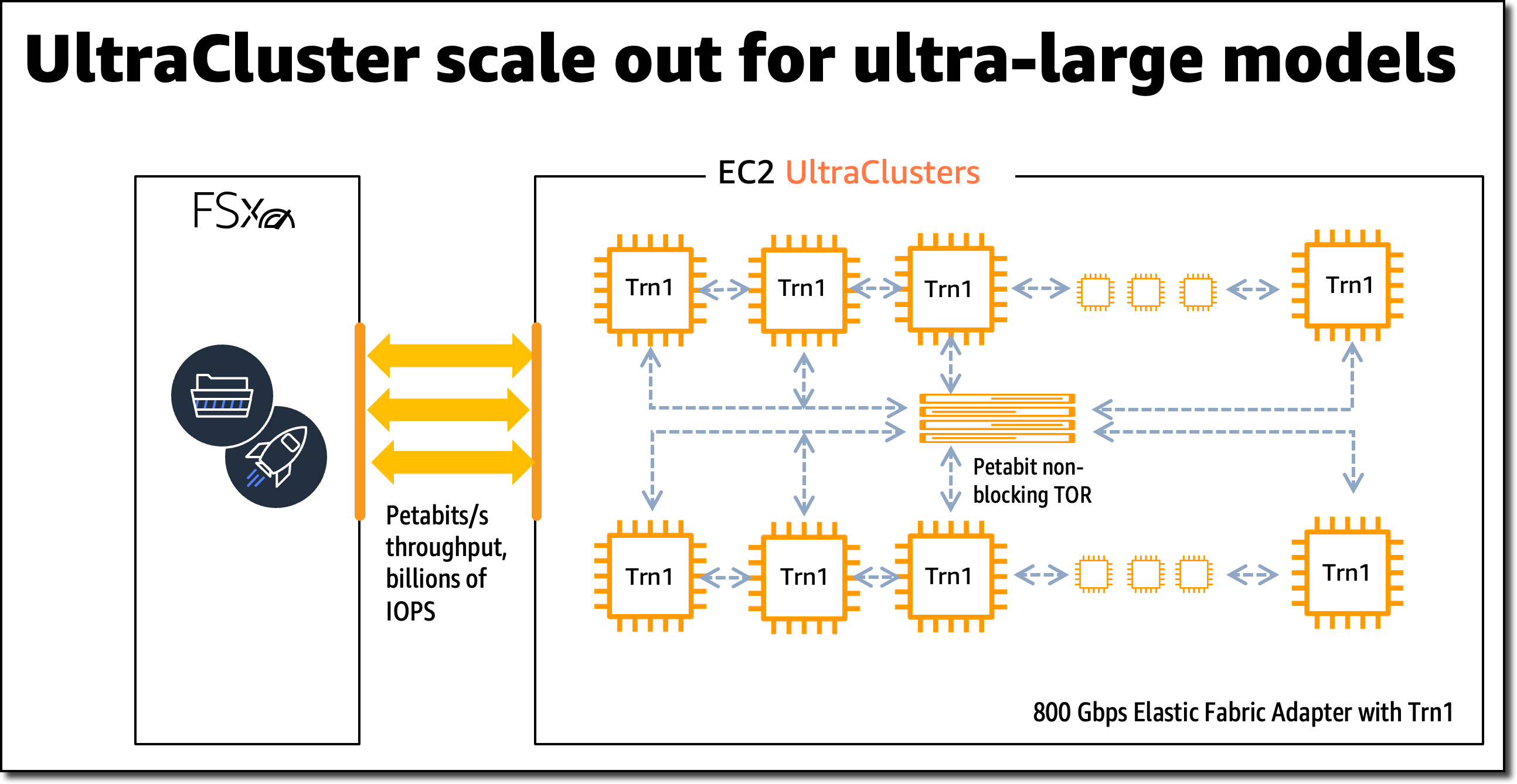
Trn1 instances are also the first EC2 instances to enable up to 800 Gbps of Elastic Fabric Adapter (EFA) network bandwidth for high-throughput network communication. This second generation EFA delivers lower latency and up to 2x more network bandwidth compared to the previous generation. Trn1 instances also come with up to 8 TB of local NVMe SSD storage for ultra-fast access to large datasets.

The following table lists the sizes and specs of Trn1 instances in detail.

Instance Name
vCPUs AWS Trainium Chips Accelerator Memory NeuronLink Instance Memory Instance Networking Local Instance Storage
trn1.2xlarge 8 1 32 GB N/A 32 GB Up to 12.5 Gbps 1x 500 GB NVMe
trn1.32xlarge 128 16 512 GB Supported 512 GB 800 Gbps 4x 2 TB NVMe

Trn1 EC2 UltraClusters
For large-scale model training, Trn1 instances integrate with Amazon FSx for Lustre high-performance storage and are deployed in EC2 UltraClusters. EC2 UltraClusters are hyperscale clusters interconnected with a non-blocking petabit-scale network. This gives you on-demand access to a supercomputer to cut model training time for large and complex models from months to weeks or even days.

Amazon EC2 Trn1 UltraCluster

AWS Trainium Innovation
AWS Trainium chips include specific scalar, vector, and tensor engines that are purpose-built for deep learning algorithms. This ensures higher chip utilization as compared to other architectures, resulting in higher performance.

Here is a short summary of additional hardware innovations:

  • Data Types: AWS Trainium supports a wide range of data types, including FP32, TF32, BF16, FP16, and UINT8, so you can choose the most suitable data type for your workloads. It also supports a new, configurable FP8 (cFP8) data type, which is especially relevant for large models because it reduces the memory footprint and I/O requirements of the model.
  • Hardware-Optimized Stochastic Rounding: Stochastic rounding achieves close to FP32-level accuracy with faster BF16-level performance when you enable auto-casting from FP32 to BF16 data types. Stochastic rounding is a different way of rounding floating-point numbers, which is more suitable for machine learning workloads versus the commonly used Round Nearest Even rounding. By setting the environment variable NEURON_RT_STOCHASTIC_ROUNDING_EN=1 to use stochastic rounding, you can train a model up to 30 percent faster.
  • Custom Operators, Dynamic Tensor Shapes: AWS Trainium also supports custom operators written in C++ and dynamic tensor shapes. Dynamic tensor shapes are key for models with unknown input tensor sizes, such as models processing text.

AWS Trainium shares the same AWS Neuron SDK as AWS Inferentia, making it easy for everyone who is already using AWS Inferentia to get started with AWS Trainium.

For model training, the Neuron SDK consists of a compiler, framework extensions, a runtime library, and developer tools. The Neuron plugin natively integrates with popular ML frameworks, such as PyTorch and TensorFlow.

The AWS Neuron SDK supports just-in-time (JIT) compilation, in addition to ahead-of-time (AOT) compilation, to speed up model compilation, and Eager Debug Mode, for a step-by-step execution.

To compile and run your model on AWS Trainium, you need to change only a few lines of code in your training script. You don’t need to tweak your model or think about data type conversion.

Get Started with Trn1 Instances
In this example, I train a PyTorch model on an EC2 Trn1 instance using the available PyTorch Neuron packages. PyTorch Neuron is based on the PyTorch XLA software package and enables conversion of PyTorch operations to AWS Trainium instructions.

Each AWS Trainium chip includes two NeuronCore accelerators, which are the main neural network compute units. With only a few changes to your training code, you can train your PyTorch model on AWS Trainium NeuronCores.

SSH into the Trn1 instance and activate a Python virtual environment that includes the PyTorch Neuron packages. If you’re using a Neuron-provided AMI, you can activate the preinstalled environment by running the following command:

source aws_neuron_venv_pytorch_p36/bin/activate

Before you can run your training script, you need to make a few modifications. On Trn1 instances, the default XLA device should be mapped to a NeuronCore.

Let’s start by adding the PyTorch XLA imports to your training script:

import torch, torch_xla
import torch_xla.core.xla_model as xm

Then, place your model and tensors onto an XLA device:

model.to(xm.xla_device())
tensor.to(xm.xla_device())

When the model is moved to the XLA device (NeuronCore), subsequent operations on the model are recorded for later execution. This is XLA’s lazy execution which is different from PyTorch’s eager execution. Within the training loop, you have to mark the graph to be optimized and run on the XLA device using xm.mark_step(). Without this mark, XLA cannot determine where the graph ends.

...
for data, target in train_loader:
	output = model(data)
	loss = loss_fn(output, target)
	loss.backward()
	optimizer.step()
	xm.mark_step()
...

You can now run your training script using torchrun <my_training_script>.py.

When running the training script, you can configure the number of NeuronCores to use for training by using torchrun –nproc_per_node.

For example, to run a multi-worker data parallel model training on all 32 NeuronCores in one trn1.32xlarge instance, run torchrun --nproc_per_node=32 <my_training_script>.py.

Data parallel is a strategy for distributed training that allows you to replicate your script across multiple workers, with each worker processing a portion of the training dataset. The workers then share their result with each other.

For more details on supported ML frameworks, model types, and how to prepare your model training script for large-scale distributed training across trn1.32xlarge instances, have a look at the AWS Neuron SDK documentation.

Profiling Tools
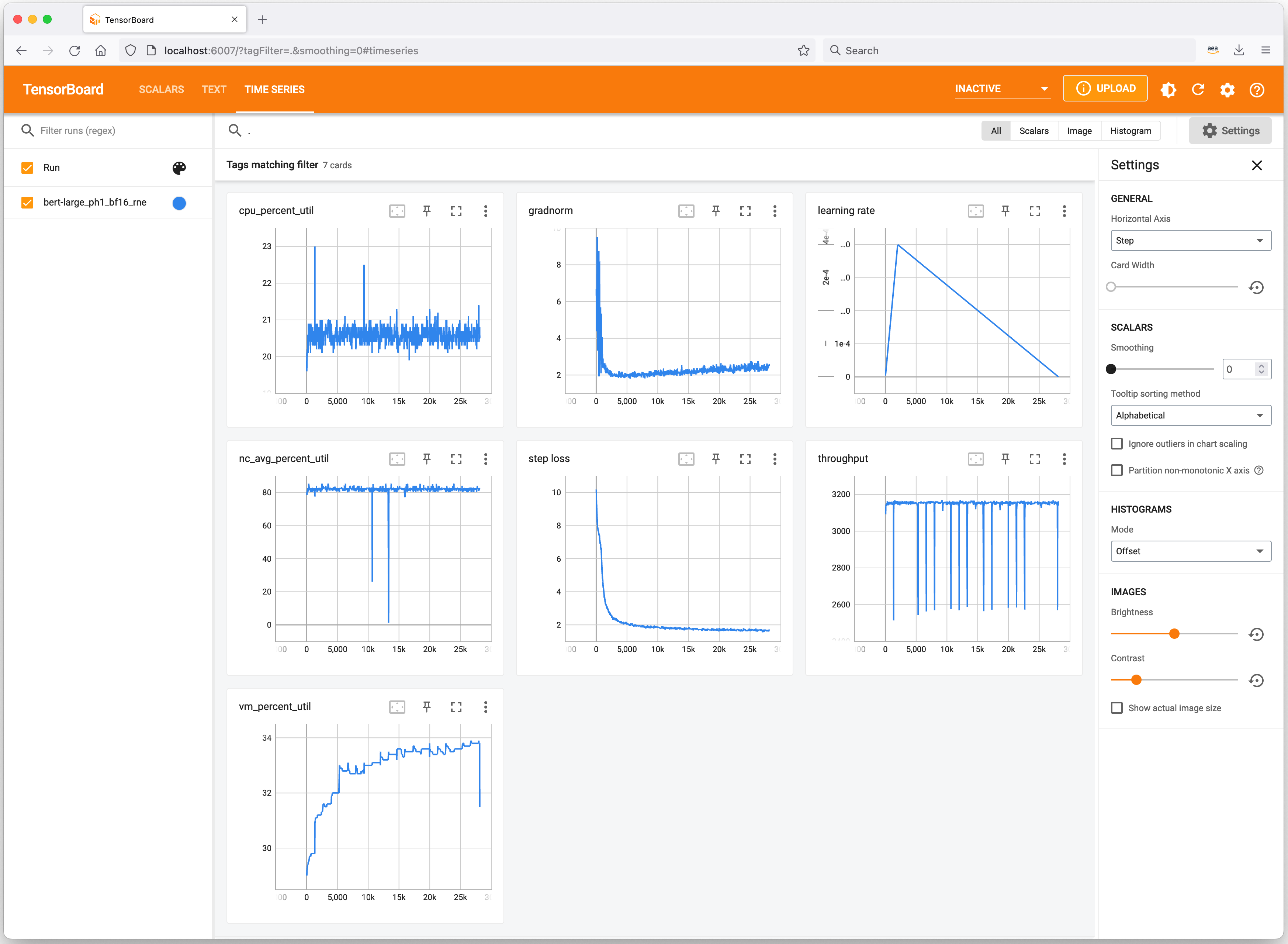
Let’s have a quick look at useful tools to keep track of your ML experiments and profile Trn1 instance resource consumption. Neuron integrates with TensorBoard to track and visualize your model training metrics.

AWS Neuron SDK TensorBoard integration

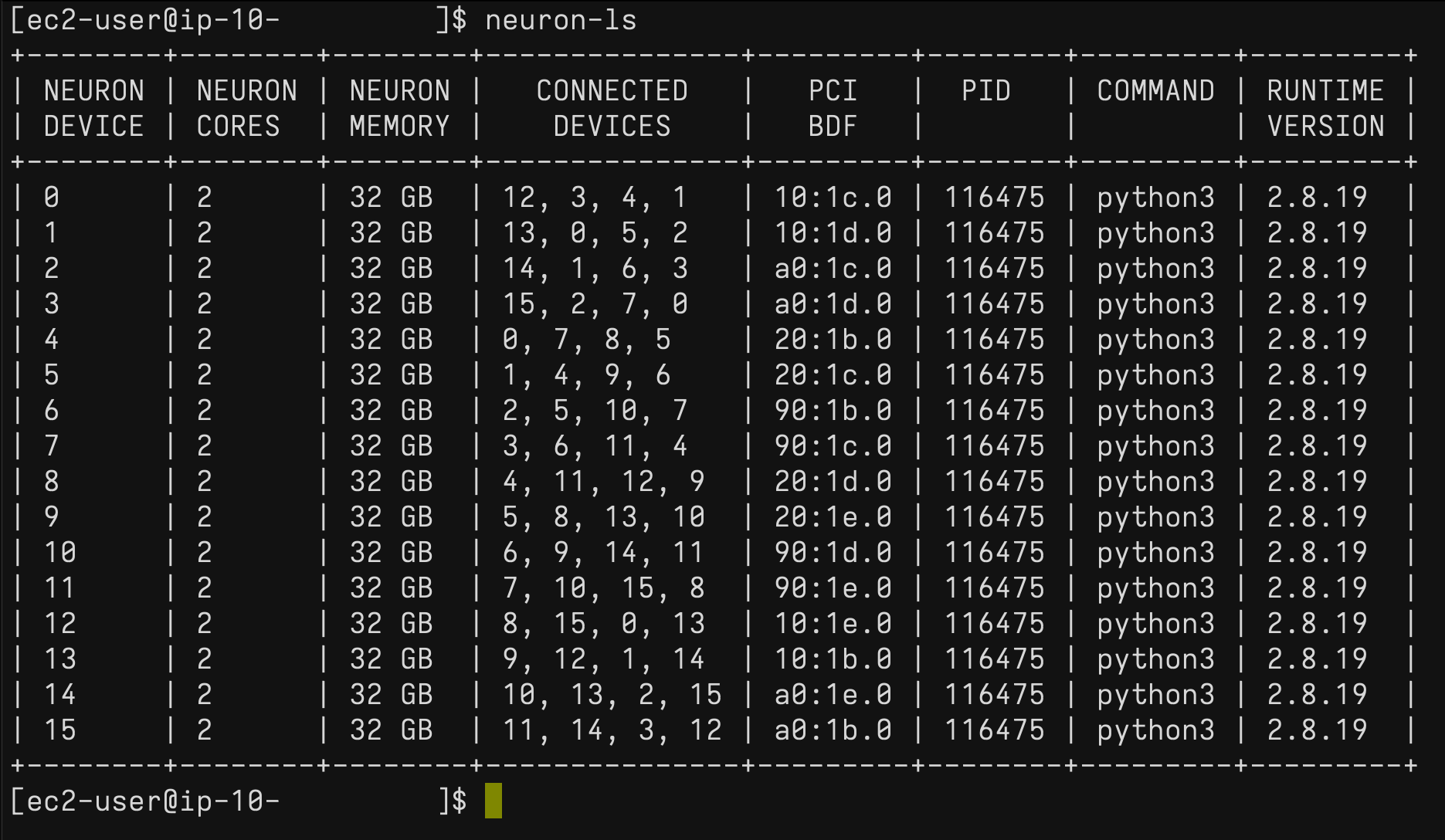
On the Trn1 instance, you can use the neuron-ls command to describe the number of Neuron devices present in the system, along with the associated NeuronCore count, memory, connectivity/topology, PCI device information, and the Python process that currently has ownership of the NeuronCores:

AWS Neuron SDK neuron-ls command

Similarly, you can use the neuron-top command to see a high-level view of the Neuron environment. This shows the utilization of each of the NeuronCores, any models that are currently loaded onto one or more NeuronCores, process IDs for any processes that are using the Neuron runtime, and basic system statistics relating to vCPU and memory usage.

AWS Neuron SDK neuron-top command

Available Now
You can launch Trn1 instances today in the AWS US East (N. Virginia) and US West (Oregon) Regions as On-Demand, Reserved, and Spot Instances or as part of a Savings Plan. As usual with Amazon EC2, you pay only for what you use. For more information, see Amazon EC2 pricing.

Trn1 instances can be deployed using AWS Deep Learning AMIs, and container images are available via managed services such as Amazon SageMaker, Amazon Elastic Kubernetes Service (Amazon EKS), Amazon Elastic Container Service (Amazon ECS), and AWS ParallelCluster.

To learn more, visit our Amazon EC2 Trn1 instances page, and please send feedback to AWS re:Post for EC2 or through your usual AWS Support contacts.

— Antje

Design a data mesh with event streaming for real-time recommendations on AWS

Post Syndicated from Vittorio Denti original https://aws.amazon.com/blogs/big-data/design-a-data-mesh-with-event-streaming-for-real-time-recommendations-on-aws/

This blog post was co-authored with Federico Piccinini.

The data landscape has been changing in recent years: there is a proliferation of entities producing and consuming large quantities of data within companies, and for most of them defining a proper data strategy has become of fundamental importance. A modern data strategy gives you a comprehensive plan to manage, access, analyze, and act on data.

As a result, more companies are considering the adoption of a data mesh architecture, a recently introduced paradigm where data is organized by domain, clear ownership of data and technology stack is enhanced, and a more agile setup is achieved. Because of this, some of your applications may need to be designed for a data-by-domain separation in order to benefit from a data mesh architecture.

In this post, we show you how to design a data mesh architecture for a scenario that requires real-time recommendations. The recommendation system is implemented through Amazon Personalize, a fully managed machine learning (ML) service, and works by consuming data by domain. For recommendations use cases, it’s important to have access to information about users, items, and interactions, often associated with different data sources within a company.

Because ML applications may have multiple types of input data, we propose a solution that works both for data at rest as well as real-time streaming. Real-time recommendations require streaming data in order to adapt to the user’s current intent.

Throughout the post, we introduce the data mesh paradigm and then extend it to a real-time use case by adding event streaming capabilities. We use the use case of a music streaming company that offers its customers the opportunity to listen to on-demand songs. The company has also started to offer, through the same platform, on-demand podcasts, and wants to take advantage of a modern data architecture to support data access for fast ML experimentation and inference.

Data mesh: A paradigm shift

Domain-driven design (DDD) represents a software design approach where complex solutions are divided into domains according to the underlying business logic. An architectural style that is often mentioned in the context of DDD is microservice architecture, a concept where software systems are structured into loosely coupled entities, namely microservices, each one owned by a small team and structured around business requirements. These paradigms, together with the advancement of cloud technologies, allowed companies to release software updates faster and continuously adapt their technology stack to evolving business requirements.

However, unlike software architectures, most data architectures were still designed around technologies rather than business domains. This changed in 2019, when Zhamak Dehghani introduced the data mesh. Data mesh is a paradigm shift towards data being treated as a product and processed as part of a domain. Data mesh applies the principles of DDD to data architectures: data is organized into data domains and the data is considered the product that the team owns and offers for consumption. This is a shift from a centralized ownership model to a decentralized one that allows companies to access data at scale. This shift also allows each team assigned to a data domain to build the data products by choosing the right technology for their job, analogous to software engineers working on a microservice.

Data mesh advocates for decentralized ownership and delivery of data management systems, while emphasizing the need for distributed governance and self-service tooling. The data mesh approach enables better autonomy of data domain owners and brings domains together to enable data sharing and federation across business units, without compromising on data security. This type of architecture supports the idea of distributed data, where all data is accessible for those with the right authority to access it. One key differentiator between a data lake and a data mesh is that in a data mesh, data doesn’t have to be consolidated into a single data lake and can remain within different databases.

For more information about the details and advantages of adopting the data mesh as a domain-driven data architecture, refer to Design a data mesh architecture using AWS Lake Formation and AWS Glue.

The components of a data mesh

Now that we have a good understanding of the data mesh paradigm, let’s look at the implementation and its components.

First, we start with data producers. These are the entities that are responsible for maintaining, owning, and exposing the specific data of their domain. Because of the domain separation, each producer can choose its own technology stack independently.

Similarly, we also have data consumers. These components, as their name indicates, use one or more data sources exposed by the producers. As before, adopting a data mesh architecture implies that each consumer is independent one another, meaning they could implement different technology stacks as well as solve different use cases.

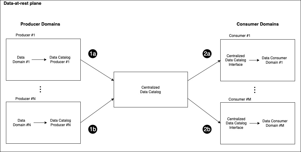
The data-at-rest plane is then completed by the Centralized Data Catalog, a component that works as the link between producers and consumers. This middle layer is responsible for indexing the available data producers into a centralized data catalog as well as controlling access to the different data sources.

The data catalog is used by the producers to expose the data products (steps 1a and 1b) to the organization’s data scientists and data engineers working on the consumer domains. The following figure illustrates how data products should be easily discoverable: the central data catalog allows the data consumers to find their data source of interest (steps 2a and 2b) after they have been registered with the centralized catalog by their corresponding producer domain (steps 1a and 1b).

Working with real-time events

One could argue that this architecture can only support data at rest as it is; indeed, there is no straightforward solution to move data in real time from a producer domain to a consumer. The paradigm presented so far addresses the scenario of data at rest, where producers are pulling data on demand rather than being notified when data is changed.

Because several applications need to quickly respond to the changes happening in the environment, real-time data is an important consideration in data architectures. For example, an ecommerce platform or a video streaming service can extract value from the real-time user interactions with content. In these cases, it’s critical to track events as they happen, feed them in the ML model, and adapt the predictions accordingly.

In this section, we want to introduce some of the streaming platforms that can work to implement this pattern, with a focus on Apache Kafka because it’s frequently used and many companies are moving their Kafka workloads to the cloud.

Apache Kafka is an open-source distributed event streaming platform that captures data in real time from sources such as microservices or databases, stores the events in streams organized into topics, and reacts to these events in real time as well as retrospectively. Event streaming architectures built on Apache Kafka follow the publish/subscribe paradigm: the producers publish events to topics via a write operation, and the consumers, which subscribe to such topics, receive the events as they happen. An alternative to Apache Kafka in this scenario could be Amazon Kinesis Data Streams, a streaming service that allows developers to collect, store, and process real-time data in the cloud.

If we consider for example an ecommerce platform, we could have a Payment microservice running the payment functionalities of the system publishing events to Purchases topic, tracking every transaction happening on the platform. Then, we could have another component subscribing to the Purchases topic to receive the events and take action accordingly, for example by updating a dashboard for business intelligence. For more information on Apache Kafka, we recommend reading Introduction to Apache Kafka.

Event-streaming architecture

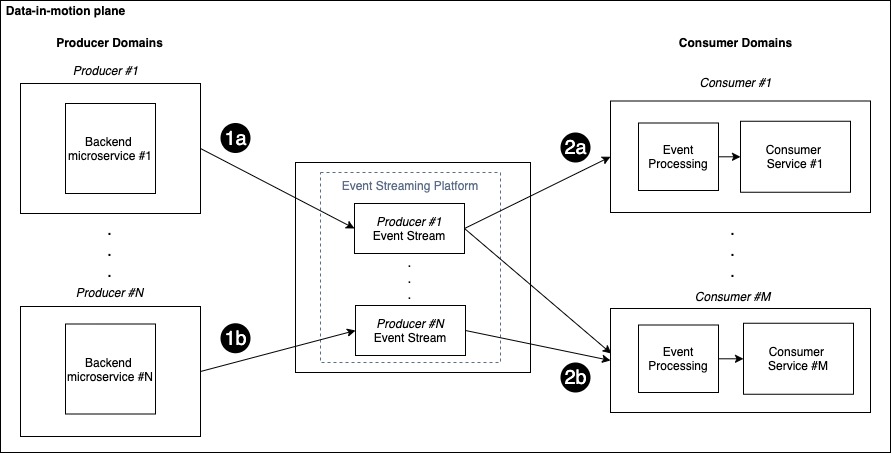
The data-in-motion plane is introduced to implement the publish/subscribe pattern in the context of a data mesh. Such a plane is composed of the set of producer and consumer domains connected via a central event streaming component that makes real-time events accessible. To benefit from the data-by-domain architecture, we consider each producer to have its own corresponding centralized stream, as shown in the following figure.

You can also think of the event stream as the channel for sending real-time events to the consumers, therefore each producer has its dedicated channel to send updates.

Each consumer can subscribe to multiple topics based on specific data needs. When new events are available, the corresponding producer publishes them in the associated stream (steps 1a and 1b) and the subscribers can read the events (step 2a and 2b), process them, and take action accordingly.

The preceding figure shows a scenario with N producer domains and M consumer domains: each consumer subscribes only to the streams of interest for that domain. In this example, Consumer #1 is subscribed to the events coming from Producer #1, while Consumer #M is subscribed to the events coming from both Producer #1 and Producer #N.

You could adopt this pattern to solve several use cases and data domains. For instance, a user playing a song on a music streaming platform can generate a new event sent from the Interactions service producer to the Personalization consumer, where the recommendation system generates personalized recommendations. Similarly, a Payment producer can send a transaction request, and a Fraud Detector consumer determines whether the transaction is fraudulent or not.

For producers and consumers to communicate correctly, the event payload schema needs to be consistent. Applications depend on schemas so no changes made to events break the implicit contract between producers and consumers. For complex use cases, you can use a schema registry to enforce compatibility in event streaming. For more information about the options for working with the AWS Glue Schema Registry, refer to Validate streaming data over Amazon MSK using schemas in cross-account AWS Glue Schema Registry.

Recommendation use case

Previously, we introduced the overall idea behind the data mesh architecture without focusing on a specific use case. In this section, we present a real-world scenario where the mesh paradigm is implemented using AWS.

Let’s consider the music streaming company XYZ, which offers its customers the opportunity to listen to on-demand songs. XYZ has recently started to offer, through the same platform, on-demand podcasts as well.

The ML team is interested in adding podcasts to the catalog of personalized recommendations that are presented to users. To do so, the ML team working on the recommendation system, which in the data mesh paradigm can be seen as a consumer, needs access to multiple data domains (producers): Users, Songs, Podcasts, and Interactions.

In this post, we use Amazon Personalize as a fully managed ML service for personalized recommendations. It allows developers to train, tune, and deploy custom ML models to deliver highly customized experiences. Amazon Personalize provisions the infrastructure and manages the entire ML pipeline, including processing the data; identifying features; and training, optimizing, and hosting the models. You can learn more about Amazon Personalize in the Developer Guide.

We now dive deeper into the implementation of the solution, both for the data-at-rest and data-in-motion scenario. ML needs large amounts of data at rest to create a dataset and train the models. Additionally, the personalization scenario requires access to real-time data to adapt to the users’ current intent, so we need access to real-time events and interactions. A data mesh solution for this scenario will require both:

  • Data at rest – Historical data from user, items, and interactions. Some of this could be stored in separate systems and data sources.
  • Data in motion – This data is for the real-time events, for instance songs listened to or new items made available in the catalog.

Architecture for data at rest

In this section, we focus on the data at rest part of the solution.

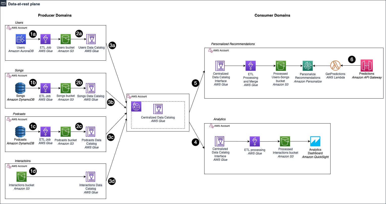
The following diagram shows how we can implement the data mesh architecture in the context of personalized recommendations, and include the podcasts in the recommendation system deployed with Amazon Personalize. Each producer domain owns the data and exposes them via the data catalogs. The consumers use the data catalogs to find the data they need for their application.

First, we can identify the three main components of the mesh architecture introduced before: data producers, the centralized data catalog, and data consumers.

In this specific example, we can see how different producer domains implement different storage solutions:

  • The Users domain uses Amazon Aurora as its own line of business (LOB) database, a relational database (step 1a)
  • Songs and Podcasts use Amazon DynamoDB, a NoSQL database (steps 1b and 1c)
  • Interactions ingests the events directly into Amazon S3 (step 1d)

The producer domains are decoupling their LOB databases from the data catalogs by using Amazon Simple Storage Service (Amazon S3). With the data mesh paradigm, each producer considers the data as a product, therefore it can preprocess the data before exposing them, and store the results in a format that is suitable for the consumers. This decoupling is implemented using AWS Glue to define an extract, transform, and load (ETL) pipeline, whose results are eventually stored in S3 buckets (steps 2a, 2b, 2c).

Finally, each producer shares its respective AWS Glue Data Catalog with the Centralized Data Catalog (steps 3a, 3b, 3c, 3d).

Data consumers can now access the different data domains through the central catalog. As shown in the preceding figure, we have two consumers: the Analytics domain, which accesses certain catalogs and showcases metrics on an Amazon QuickSight dashboard (step 4), and the Personalized Recommendations domain (step 5).

The latter, which is the one of interest for this post, consists of an AWS Glue ETL job that accesses, through the central catalog, data from the different producers. The ETL job performs traditional data engineering tasks, for example merging song and podcast data. We can now generate our Amazon Personalize solution, where our items dataset includes information about both songs and podcasts, expanding the initial recommendation catalog.

Our recommendation engine is then made available for inference requests through an API deployed using Amazon API Gateway (step 6).

The architecture is designed to work across multiple accounts: an AWS account is a natural boundary for the resources deployed into it and a single unit of billing. This approach allows us to separate the resources owned by the different domains and maintain operational agility: each team owns and controls its account. To learn more about the approaches for sharing data catalogs across different accounts while working with a data mesh, check out Design a data mesh architecture using AWS Lake Formation and AWS Glue.

We’re now able to provide users with song or podcast recommendations based on their comprehensive listening preferences across the two categories. In the next section, we explore how to improve the architecture to be reactive to continuously evolving data, such as new songs added to the catalog or new interactions made available.

Architecture for data in motion

Earlier, we introduced the theoretical framework for event streaming in the context of the data mesh, defined as the data-in-motion plane. We can now drill down into the architecture for our specific use case.

We’re using a scenario with four producers (Users, Songs, Podcasts, and Interactions), the central streaming component, and two consumer domains (Personalized Recommendations and Analytics). The data-in-motion plane is implemented by using a platform for event streaming, namely Apache Kafka, and each producer has a dedicated stream to publish its events.

In the scenario of real-time recommendations for music, the Personalized Recommendations consumer is notified about changes to Users, Songs, Podcasts, and Interactions. Similar to the at-rest example, we also consider a second consumer domain, called Analytics, used to create real-time dashboards about the trends in the interactions. Here, the analytics consumer requires only interaction events, therefore it subscribes only to the Interactions stream.

This architecture is designed to offer a loosely coupled interaction mechanism for producers and consumers: the producers don’t need to know about the consumers that are part of the system. The producers focus on emitting the events, the events are sent to the data-in-motion plane, and the delivery is guaranteed by the streaming platform.

Let’s drill down into the strategy for building this architecture in the cloud. For readability purposes, we study this part of the solution in isolation, without adding to the diagram of the data-at-rest scenario.

From a technological perspective, we use AWS Lambda to run the back-end business logic of the application: the microservice runs the logic in a Lambda function and publishes events to the event streams. We use Lambda because it fits our use case well, both for scalability and operational efficiency, because it offers minimal operational overhead. However, the architecture pattern is also valid for other types of backend deployments, for example, containers running on Amazon Elastic Kubernetes Service (Amazon EKS) or Amazon Elastic Container Service (Amazon ECS).

The data-in-motion plane is implemented using Amazon Managed Streaming for Apache Kafka (Amazon MSK), a fully managed solution for running Apache Kafka in the cloud. It provisions the servers, configures the Apache Kafka clusters, replaces servers when they fail, orchestrates server patches and upgrades, and runs clusters for high availability. Kafka organizes and stores events into topics. Topics are always multi-producer and multi-consumer: this means that one or many producers can publish to the same topic, and one or many consumers can subscribe to read from the topic. We use the concept of topics to model this architecture paradigm, and we assign one topic for each producer domain.

Finally, we adapt our previously introduced consumer domain, Personalized Recommendations, to take into account real-time events. This time, we use Lambda to read the events from the topics and invoke the commands to call the Amazon Personalize API through the Amazon Personalize SDK. Within the same consumer domain, we use a Lambda function per topic, which is triggered as soon as a new event is published in the monitored topic. This event-driven pattern allows us to run code only when a new event is published and we need to update the information in Amazon Personalize. Each Lambda function in the Personalized Recommendations domain uses the Amazon Personalize SDK to invoke the corresponding actions on Amazon Personalize and update the datasets.

Let’s consider a new interaction happening in the system using the following figure. This serverless implementation of the event streaming pattern extends the data mesh to respond to real-time events.

The Interactions microservice, which is running the backend logic of the application, publishes a new event (step 1), which is persisted in the Interactions topic (step 2). The publishing of a new event triggers the Lambda functions subscribed to the topic, in this case InteractionsUpdate and InteractionsIngestor (step 3). The InteractionsUpdate function invokes the PutEvents operation on the Amazon Personalize API through the Amazon Personalize SDK to add the real-time event to the recommendation system (step 4). InteractionsIngestor triggers the operations to refresh the dashboards according to the strategy adopted by the Analytics domain. Finally, other services and components can consume the recommendations through the API exposed by the Personalized Recommendation domain to make the predictions consumable (step 5).

For the Analytics domain, which we added to showcase the scalability of this architecture, we use a Lambda function to ingest the real-time events into Amazon Kinesis Data Firehose. Then we can visualize the interactions using Amazon OpenSearch Service in conjunction with Amazon QuickSight. For more details, refer to Visualize live analytics from Amazon QuickSight connected to Amazon OpenSearch Service.

Because the data producers, Kafka resources, and data consumers are all in different accounts, we need to establish cross-account connectivity to keep the traffic within the AWS infrastructure and avoid the public internet, both for security reasons as well as cost-optimization. The objective of this post is to show the architecture and the approach to implement this pattern. If you want to dive deeper into how to establish cross-account connectivity between producers and consumers and Amazon MSK, refer to Secure connectivity patterns to access Amazon MSK and How Goldman Sachs builds cross-account connectivity to their Amazon MSK clusters with AWS Private Link.

Data mesh with event streaming: Putting it all together

Earlier, we recalled the data mesh paradigm and designed a solution to emphasize the importance of adopting a data as a product strategy. Each producer domain exposes the data via the catalog, and they are made centrally discoverable through the Centralized Data Catalog. Each consumer domain has a catalog interface for connecting to the central catalog and finding the data required to build the solution the domain focuses on.

Next, we studied the scenario for data in motion, introduced Apache Kafka and Amazon MSK to implement the event streaming platform, and connected the producers and consumers with the streaming service via Lambda. This event-driven implementation allows us to decouple the producers from the consumers, and make the solution scalable as the domains may change and evolve during time, without significant changes required in the architecture.

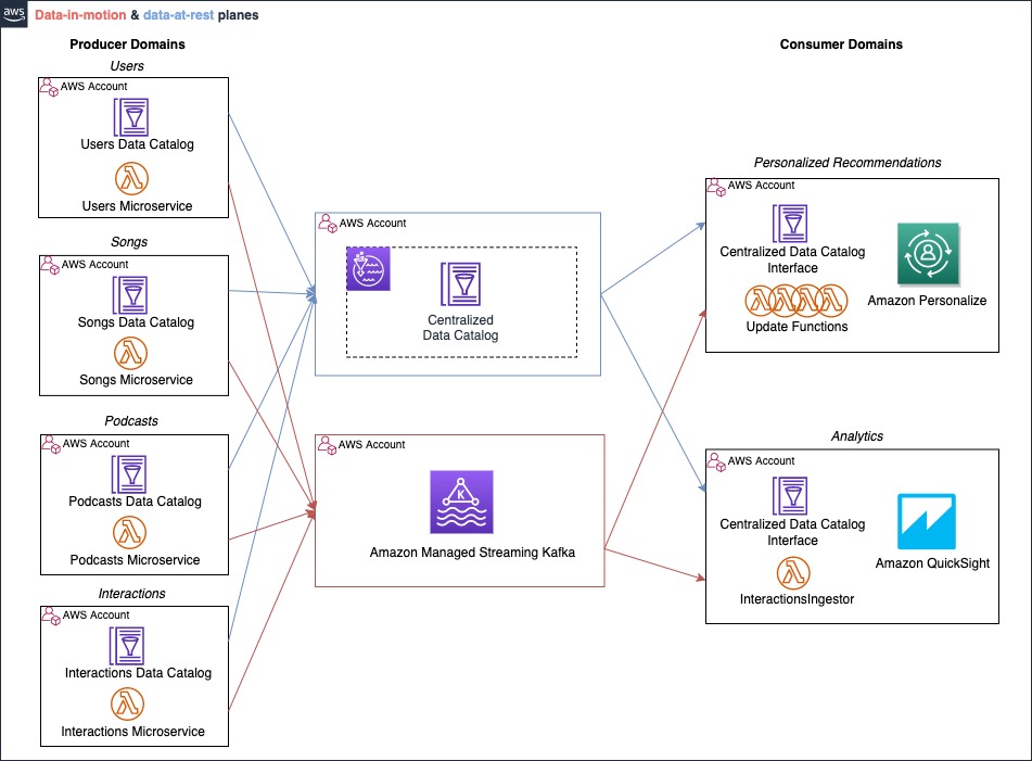
We can now put it all together, as shown in the following figure. The complete data mesh with event streaming architecture uses two different data planes: one is dedicated for sharing data at rest (blue); the other one is for data in motion (red).

Each domain has two interfaces required to communicate with both planes: the data catalogs and the Lambda functions. The data at rest is shared and discovered by taking advantage of the data catalogs, whereas the data in motion are emitted by the service running the backend logic in the producer domains. They’re consumed using the Lambda functions subscribed to the topics, which are deployed in the consumer domains.

Conclusion

In this post, we introduced the high-level architecture paradigm that allows you to extend the concept of a data mesh to real-time events.

We first covered the fundamental concepts associated with this architectural style, and then showcased how to apply this solution to solve real-world business challenges, such as real-time personalized recommendations and analytics, in a multi-account setting on AWS.

Furthermore, the framework presented in this post can be generalized to different domains, for example other AWS AI services such as Amazon Forecast or Amazon Comprehend, or your custom ML solutions built for your specific scenario and deployed through Amazon SageMaker. With the most experience, the most reliable, scalable and secure cloud, and the most comprehensive set of services and solutions, AWS is the best place to unlock value from your data.

More resources:


About the authors

Vittorio Denti is a Solutions Architect at AWS based in London. After completing his M.Sc. in Computer Science and Engineering at Politecnico di Milano (Milan) and the KTH Royal Institute of Technology (Stockholm), he joined AWS. Vittorio has a background in Distributed Systems and Machine Learning, and a strong interest in cloud technologies. He’s especially passionate for software engineering, building ML models, and putting ML into production.

Anna Grüebler is a Specialist Solutions Architect at AWS focusing on in Artificial Intelligence. She has more than 10 years experience helping customers develop and deploy machine learning applications. Her passion is taking new technologies and putting them in the hands of everyone, and solving difficult problems leveraging the advantages of using AI in the cloud.

New Hands-On Course for Business Analysts – Practical Decision Making using No-Code ML on AWS

Post Syndicated from Antje Barth original https://aws.amazon.com/blogs/aws/new-hands-on-course-for-business-analysts-practical-decision-making-using-no-code-ml-on-aws/

Artificial intelligence (AI) is all around us. AI sends certain emails to our spam folders. It powers autocorrect, which helps us fix typos when we text. And now we can use it to solve business problems.

In business, data-driven insights have become increasingly valuable. These insights are often discovered with the help of machine learning (ML), a subset of AI and the foundation of complex AI systems. And ML technology has come a long way. Today, you don’t need to be a data scientist or computer engineer to gain insights. With the help of no-code ML tools such as Amazon SageMaker Canvas, you can now achieve effective business outcomes using ML without writing a single line of code. You can better understand patterns, trends, and what’s likely to happen in the future. And that means making better business decisions!

Today, I’m happy to announce that AWS and Coursera are launching the new hands-on course Practical Decision Making using No-Code ML on AWS. This five-hour course is designed to demystify AI/ML and give anyone with a spreadsheet the ability to solve real-life business problems.

Practical Decision Making on Coursera

Course Highlights
Over the course of three lessons, you will learn how to address your business problem using ML, how to build and understand an ML model without any code, and how to use ML to extract value to make better decisions. Each lesson walks you through real-life business scenarios and hands-on exercises using Amazon SageMaker Canvas, a visual, no-code ML tool.

Lesson 1 – How To Address Your Business Problem Using ML
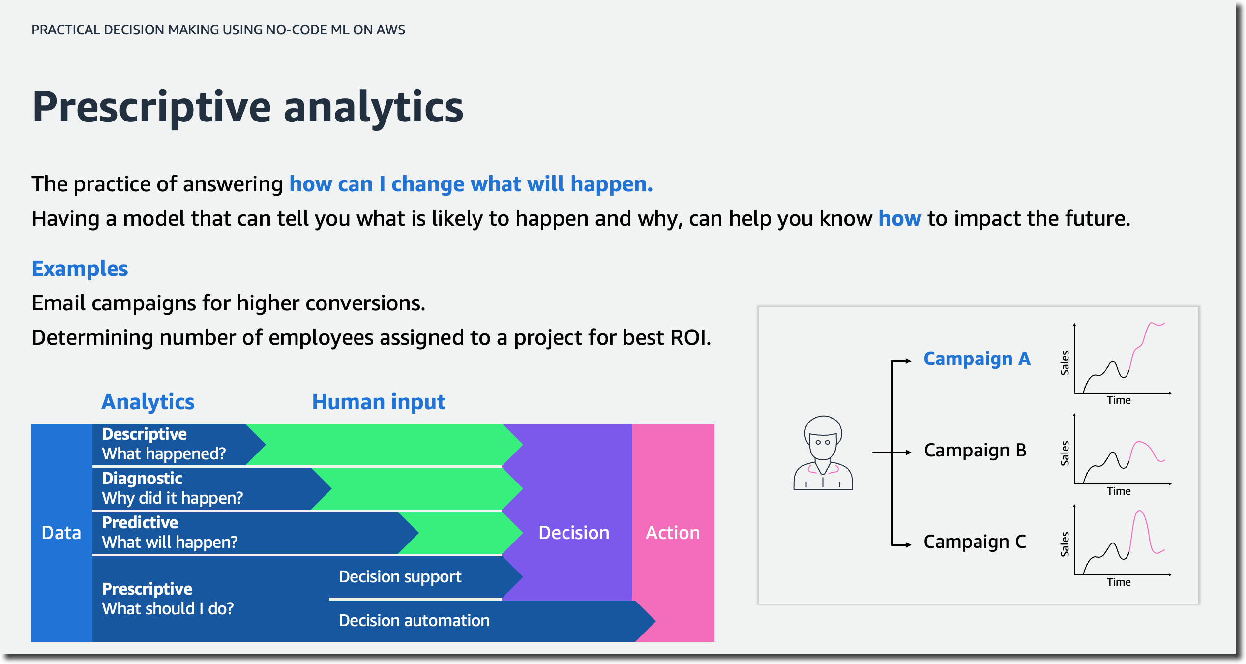
In the first lesson, you will learn how to address your business problem using ML without knowing data science. You will be able to describe the four stages of analytics and discuss the high-level concepts of AI/ML.

Practical Data Science - Prescriptive Analytics

This lesson will also introduce you to automated machine learning (AutoML) and how AutoML can help you generate insights based on common business use cases. You will then practice forming business questions around the most common machine learning problem types.

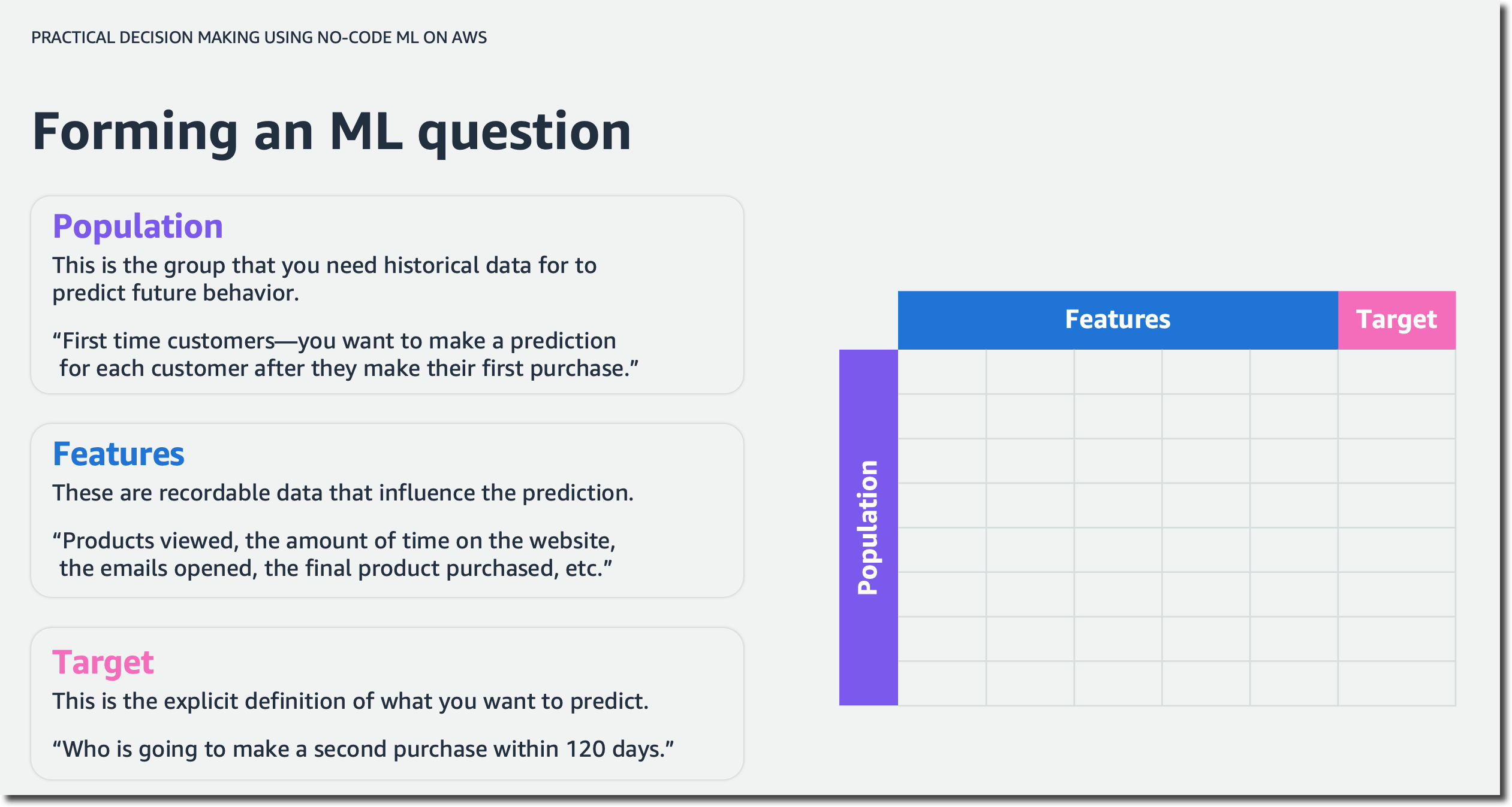
Practical Decision Making - Forming ML questions

For example, imagine you are a business analyst at a ticketing company. You manage ticket sales for large venues—concerts, sporting events, and so on. Let’s assume you want to predict cash flow. A question to solve with ML could be: “How can you better forecast ticket sales?” This is an example of time series forecasting. You will also explore numeric and category ML problems throughout the course. They will help you answer business questions such as “What’s the likely annual revenue for a customer?” and “Will this customer buy another ticket in the next three months?”.

Next, you will learn about the iterative process of asking questions for machine learning to make the questions more explicit and explore how to pick the highest value problems to work on.

Practical Decision Making - Value vs. Ease

The first lesson wraps up with a deep dive on how time influences your data across forecasting and nonforecasting business problems and how to set up your data for each ML problem type.

Lesson 2 – Build and Understand an ML Model Without Any Code
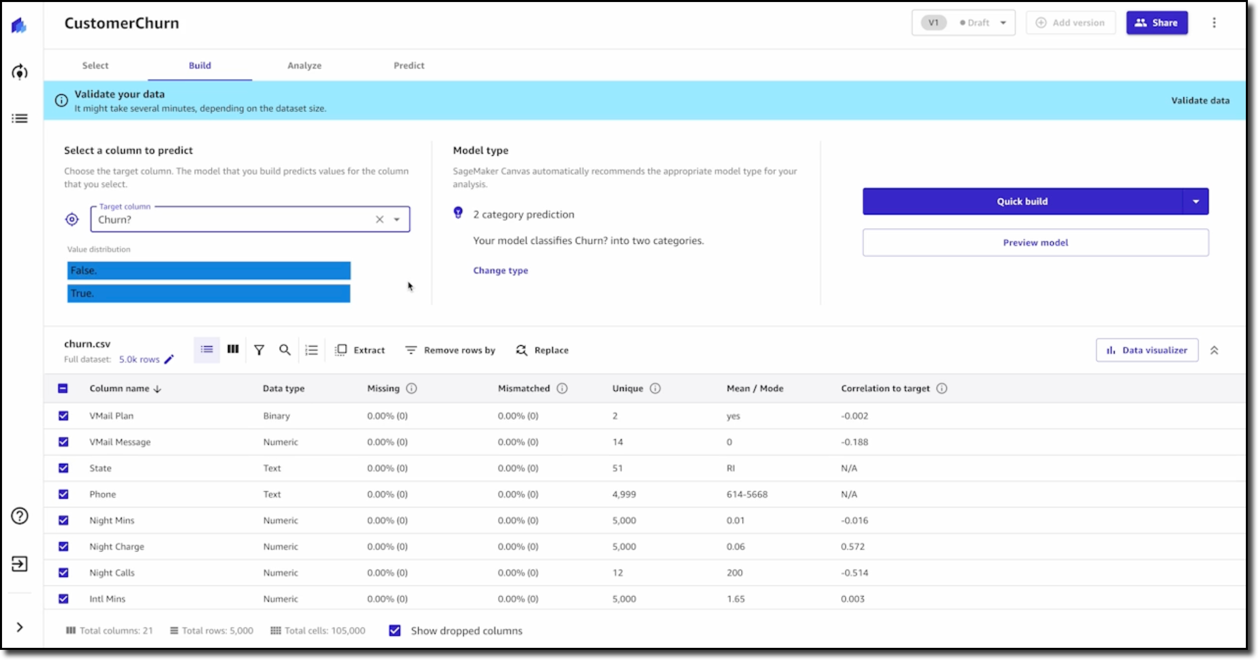
In the second lesson, you learn how to build and understand an ML model without any code using Amazon SageMaker Canvas. You will focus on a customer churn example with synthetically generated data from a cellular services company. The problem question is, “Which customers are most likely to cancel their service next month?”

Practical Decision Making - Customer Churn Example

You will learn how to import data and start exploring it. This lesson will explain how to select the right configuration, pick the target column, and show you how to prepare your data for ML.

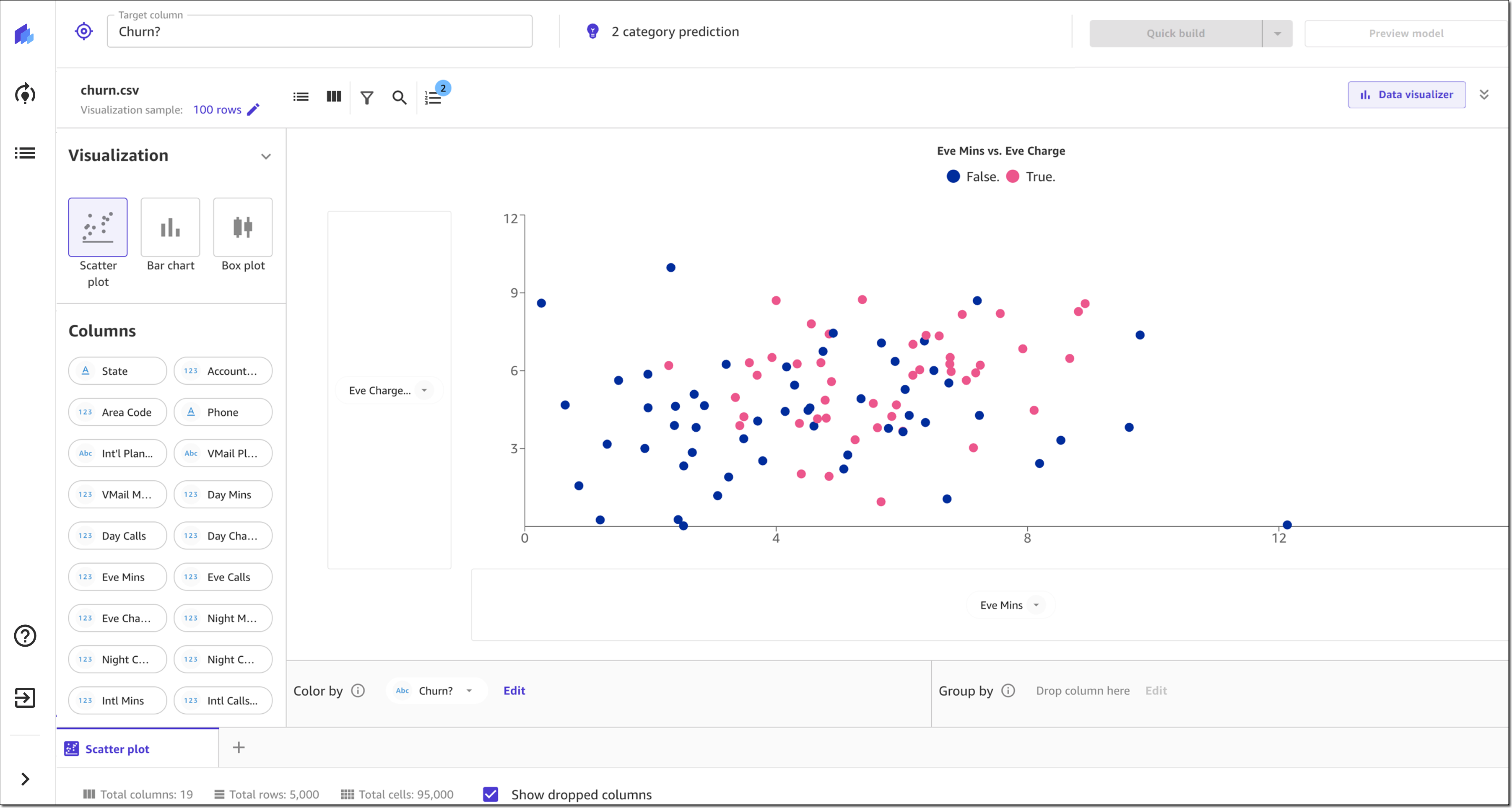
SageMaker Canvas also recently introduced new visualizations for exploratory data analysis (EDA), including scatter plots, bar charts, and box plots. These visualizations help you analyze the relationships between features in your data sets and comprehend your data better.

Practical Decision Making - SageMaker Canvas Scatter Plot

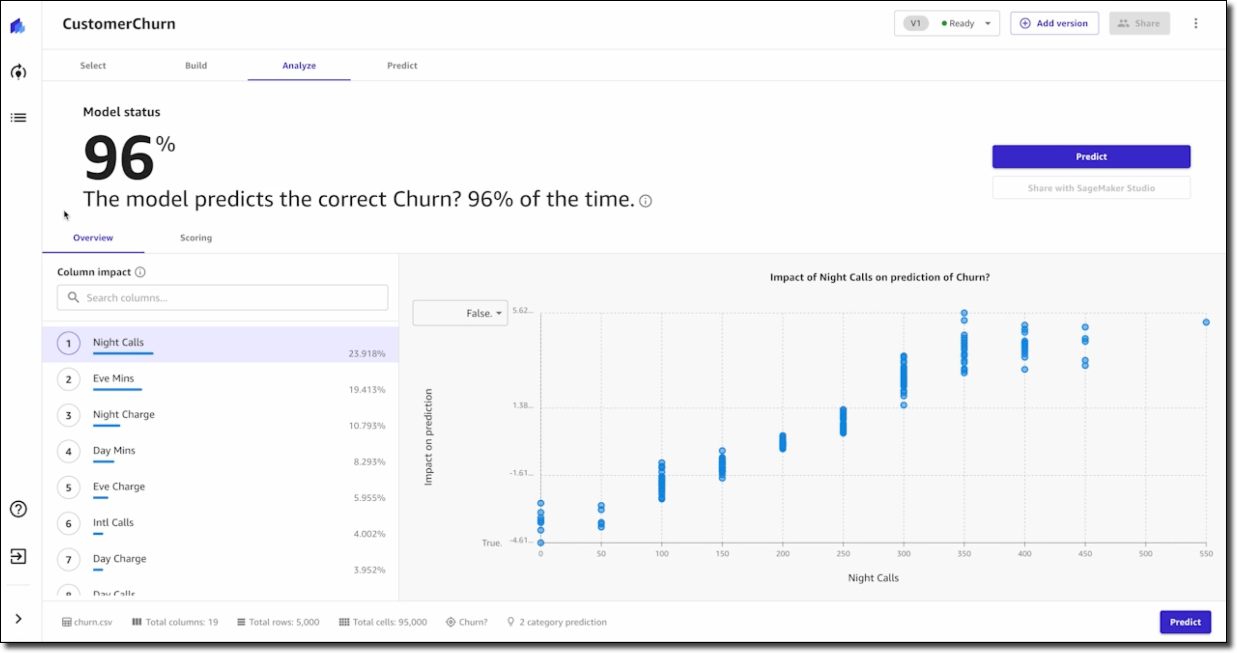
After a final data validation, you can preview the model. This shows you right away how accurate the model might be and, on average, which features or columns have the greatest relative impact on model predictions. Once you are done preparing and validating the data, you can go ahead and build the model.

Practical Decision Making - Model Evaluation

Next, you will learn how to evaluate the performance of the model. You will be able to describe the difference between training data and test data splits and how they are used to derive the model’s accuracy score. The lesson also discusses additional performance metrics and how you can apply domain knowledge to decide if the model is performing well. Once you understand how to evaluate the performance metrics, you have the foundation for making better business decisions.

The second lesson wraps up with some common gotchas to watch out for and shows how to iterate on the model to keep improving performance. You will be able to describe the concept of data leakage as a result of memorization versus generalization and additional model flaws to avoid. You will also learn how to iterate on questions, included features, and sample sizes to keep increasing model performance.

Lesson 3 – Extract Value From ML
In the third lesson, you learn how to extract value from ML to make better decisions. You will be able to generate and read predictions, including predictions on a single row of a spreadsheet, called a single prediction, and predictions on the entire spreadsheet, called batch prediction. You will be able to understand what is impacting predictions and play with different scenarios.

Next, you will learn how to share insights and predictions with others. You will learn how to take visuals from the product, such as feature importance charts or scoring diagrams, and share the insights through presentations or business reports.

The third lesson wraps up with how to collaborate with the data science team or a team member with machine learning expertise. When you build your model using SageMaker Canvas, you can choose either a Quick build or a Standard build. The Quick build usually takes 2–15 minutes and limits the input dataset to a maximum of 50,000 rows. The Standard build usually takes 2–4 hours and generally has a higher accuracy. SageMaker Canvas makes it easy to share a standard build model. In the process, you can reveal the model’s behind-the-scenes complexity down to the code level.

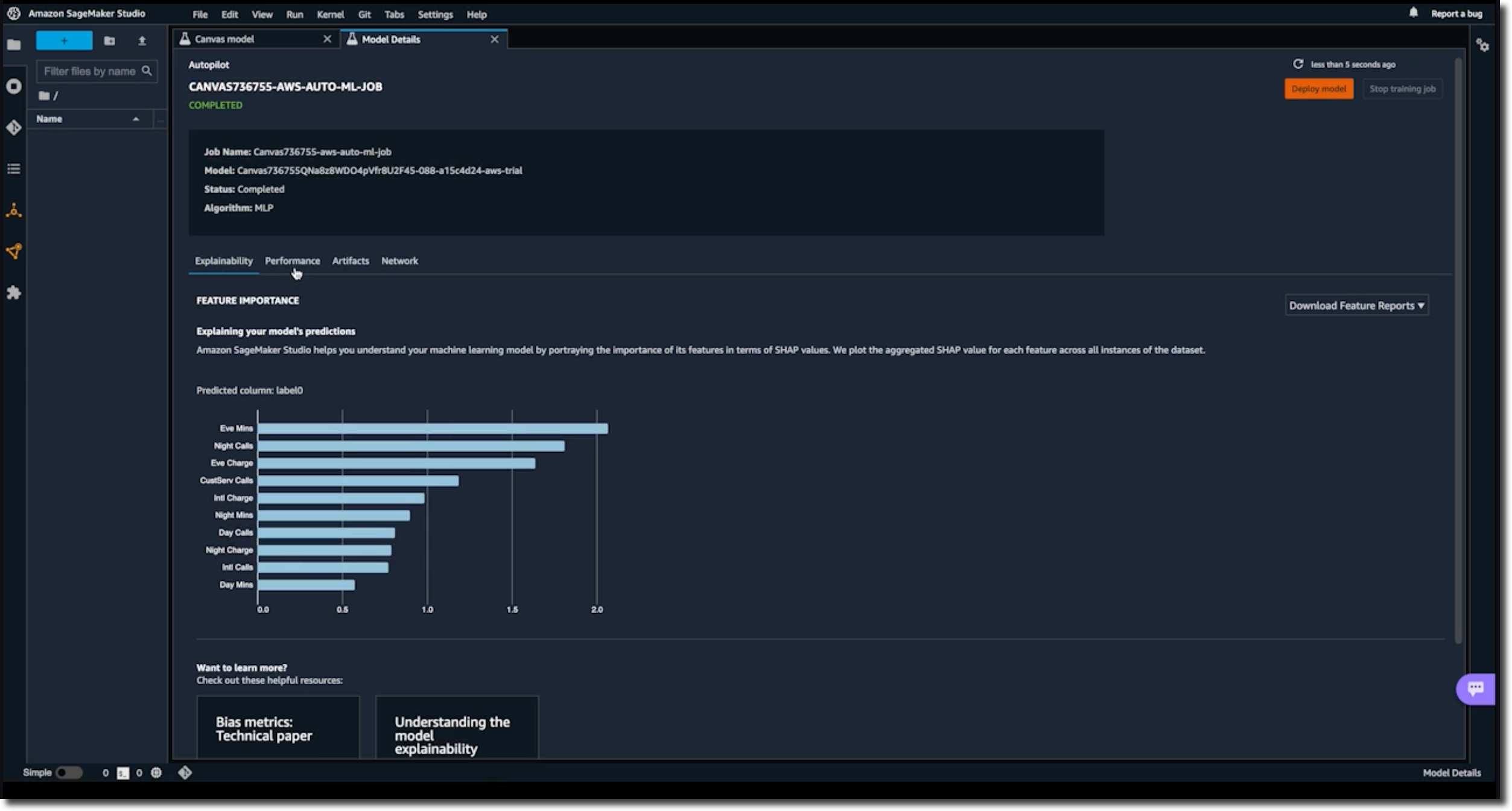
Once you have the trained model open, you can click on the Share button. This creates a link that can be opened in SageMaker Studio, an integrated development environment used by data science teams.

Practical Decision Making - Share Model

In SageMaker Studio, you can see the transformations to the input data set and detailed information about scoring and artifacts, like the model object. You can also see the Python notebooks for data exploration and feature engineering.

Practical Decision Making - SageMaker Studio

Hands-On Exercises
This course includes seven hands-on labs to put your learning into practice. You will have the opportunity to use no-code ML with SageMaker Canvas to solve real-world challenges based on publicly available datasets.

The labs focus on different business problems across industries, including retail, financial services, manufacturing, healthcare, and life sciences, as well as transport and logistics.

You will have the opportunity to work on customer churn predictions, housing price predictions, sales forecasting, loan predictions, diabetic patient readmission prediction, machine failure predictions, and supply chain delivery on-time predictions.

Register Today
Practical Decision Making using No-Code ML on AWS is a five-hour course for business analysts and anyone who wants to learn how to solve real-life business problems using no-code ML.

Sign up for Practical Decision Making using No-Code ML on AWS today at Coursera!

— Antje

Detecting Deepfake Audio by Modeling the Human Acoustic Tract

Post Syndicated from Bruce Schneier original https://www.schneier.com/blog/archives/2022/10/detecting-deepfake-audio-by-modeling-the-human-acoustic-tract.html

This is interesting research:

In this paper, we develop a new mechanism for detecting audio deepfakes using techniques from the field of articulatory phonetics. Specifically, we apply fluid dynamics to estimate the arrangement of the human vocal tract during speech generation and show that deepfakes often model impossible or highly-unlikely anatomical arrangements. When parameterized to achieve 99.9% precision, our detection mechanism achieves a recall of 99.5%, correctly identifying all but one deepfake sample in our dataset.

From an article by two of the researchers:

The first step in differentiating speech produced by humans from speech generated by deepfakes is understanding how to acoustically model the vocal tract. Luckily scientists have techniques to estimate what someone—or some being such as a dinosaur—would sound like based on anatomical measurements of its vocal tract.

We did the reverse. By inverting many of these same techniques, we were able to extract an approximation of a speaker’s vocal tract during a segment of speech. This allowed us to effectively peer into the anatomy of the speaker who created the audio sample.

From here, we hypothesized that deepfake audio samples would fail to be constrained by the same anatomical limitations humans have. In other words, the analysis of deepfaked audio samples simulated vocal tract shapes that do not exist in people.

Our testing results not only confirmed our hypothesis but revealed something interesting. When extracting vocal tract estimations from deepfake audio, we found that the estimations were often comically incorrect. For instance, it was common for deepfake audio to result in vocal tracts with the same relative diameter and consistency as a drinking straw, in contrast to human vocal tracts, which are much wider and more variable in shape.

This is, of course, not the last word. Deepfake generators will figure out how to use these techniques to create harder-to-detect fake voices. And the deepfake detectors will figure out another, better, detection technique. And the arms race will continue.

Slashdot thread.

3 Ways to Improve Data Protection in the Cloud

Post Syndicated from Jesse Mack original https://blog.rapid7.com/2022/09/07/3-ways-to-improve-data-protection-in-the-cloud/

3 Ways to Improve Data Protection in the Cloud

Cloud complexity is now a well-documented and widely felt phenomenon across technology teams — IT, development, and security alike. Multi-cloud architectures have become the norm, with 89% of organizations embracing a strategy that involves multiple cloud vendors. Not only are companies managing greater amounts of data than ever before, they’re also spread across an ever-increasing array of cloud services, applications, and devices.

Securing all this information and preventing data loss in a multi-cloud environment would be a tall task for any security team. Add to the mix an increasingly heightened threat landscape and an ongoing cybersecurity skills shortage, and the challenge becomes even greater.

Rapid7, Mimecast, and Netskope recently published a joint white paper outlining best practices for cloud data protection and pinpointing some key resources that organizations can leverage in this effort. Here are three key concepts the paper highlights.

1. Embrace AI

Artificial intelligence (AI) and machine learning are well-known technologies at this point, but their potential is only just beginning to be tapped when it comes to helping security teams become more efficient and more effective.

Examples of AI-based tools that can help security teams include curated detections within an extended detection and response (XDR) platform, as well as intelligent threat and anomaly detection within cloud security tools.

Machine learning won’t ever replace the trained eye and keen insight of a veteran cybersecurity analyst — but AI-based tools can take on some of the repetitive and time-consuming tasks that security pros face, allowing analysts to increase productivity and focus on the alerts and issues that matter most. The goal is human-machine collaboration, with AI augmenting and boosting the capabilities of the analyst.

2. Utilize automation

Automation and AI work together as a one-two punch of process improvement for security. If an AI-based tool detects an anomalous event, automation allows you to set up actions that can take place in response to that suspicious activity. This can help get the ball rolling faster on mitigating security issues — and speed is the name of the game when it comes to keeping out attackers.

In the context of a cloud security platform, built-in automation and remediation tools let you create bots that can carry out certain tasks, specified by:

  • Scope: What resources the bot should evaluate — i.e., specific cloud resource groups, or certain types of resources contained in those groups
  • Filters: The conditions in which a bot should act — e.g., what tags the resource has, or whether the ports are open
  • Actions: What task you want the bot to carry out — e.g., delete a resource, start or stop an instance, or send an email with key information about the resource in question

3. Leverage integrations

AI and automation can help drive efficiencies — but with a multitude of cloud services in play, there’s a risk that these automated actions proliferate and become unwieldy, making it tough for security teams to reap the full benefits. This is where integrations become critical: They allow teams to coordinate actions quickly and seamlessly across multiple vendor systems.

Integrations make it easier to create a holistic security environment formed by a consistent set of controls, rather than a patchwork of best practices. For example, if you have an integration that links your email security gateway to your security information and event management (SIEM) tool, you can create an alert when a user receives an email containing suspected ransomware or malware, and take automated remediation actions instantly. Or if your security service edge (SSE) platform detects a serious data exfiltration risk, you can build a customized workflow in your security orchestration, automation, and response (SOAR) to quarantine that resource or take it offline.

Dive deeper on cloud data protection

Keeping data secure in the cloud comes with its share of challenges, but integrations that leverage AI-based analytics and automated workflows can help you ensure you know where your data is, what security controls are in place, and what threats there might be in your environment.

Looking to go deeper on how to bring this vision to life? Download the white paper today, or join experts from Mimecast, Netskope, and Rapid7 for the webinar “Data Protection and Control in the Cloud” at 2pm EST on Tuesday, September 13.

Additional reading:

NEVER MISS A BLOG

Get the latest stories, expertise, and news about security today.

Classroom activities to discuss machine learning accuracy and ethics | Hello World #18

Post Syndicated from Janina Ander original https://www.raspberrypi.org/blog/classroom-activity-machine-learning-accuracy-ethics-hello-world-18/

In Hello World issue 18, available as a free PDF download, teacher Michael Jones shares how to use Teachable Machine with learners aged 13–14 in your classroom to investigate issues of accuracy and ethics in machine learning models.

Machine learning: Accuracy and ethics

The landscape for working with machine learning/AI/deep learning has grown considerably over the last couple of years. Students are now able to develop their understanding from the hard-coded end via resources such as Machine Learning for Kids, get their hands dirty using relatively inexpensive hardware such as the Nvidia Jetson Nano, and build a classification machine using the Google-driven Teachable Machine resources. I have used all three of the above with my students, and this article focuses on Teachable Machine.

For this module, I’m more concerned with the fuzzy end of AI, including how credible AI decisions are, and the elephant-in-the-room aspect of bias and potential for harm.

Michael Jones

For the worried, there is absolutely no coding involved in this resource; the ‘machine’ behind the portal does the hard work for you. For my Year 9 classes (students aged 13 to 14) undertaking a short, three-week module, this was ideal. The coding is important, but was not my focus. For this module, I’m more concerned with the fuzzy end of AI, including how credible AI decisions are, and the elephant-in-the-room aspect of bias and potential for harm.

Getting started with Teachable Machine activities

There are three possible routes to use in Teachable Machine, and my focus is the ‘Image Project’, and within this, the ‘Standard image model’. From there, you are presented with a basic training scenario template — see Hello World issue 16 (pages 84–86) for a step-by-step set-up and training guide. For this part of the project, my students trained the machine to recognise different breeds of dog, with border collie, labrador, saluki, and so on as classes. Any AI system devoted to recognition requires a substantial set of training data. Fortunately, there are a number of freely available data sets online (for example, download a folder of dog photos separated by breed by accessing helloworld.cc/dogdata). Be warned, these can be large, consisting of thousands of images. If you have more time, you may want to set students off to collect data to upload using a camera (just be aware that this can present safeguarding considerations). This is a key learning point with your students and an opportunity to discuss the time it takes to gather such data, and variations in the data (for example, images of dogs from the front, side, or top).

Drawing of a machine learning ars rover trying to decide whether it is seeing an alien or a rock.
Image recognition is a common application of machine learning technology.

Once you have downloaded your folders, upload the images to your Teachable Machine project. It is unlikely that you will be able to upload a whole subfolder at once — my students have found that the optimum number of images seems to be twelve. Remember to build this time for downloading and uploading into your lesson plan. This is a good opportunity to discuss the need for balance in the training data. Ask questions such as, “How likely would the model be to identify a saluki if the training set contained 10 salukis and 30 of the other dogs?” This is a left-field way of dropping the idea of bias into the exploration of AI — more on that later!

Accuracy issues in machine learning models

If you have got this far, the heavy lifting is complete and Google’s training engine will now do the work for you. Once you have set your model on its training, leave the system to complete its work — it takes seconds, even on large sets of data. Once it’s done, you should be ready to test you model. If all has gone well and a webcam is attached to your computer, the Output window will give a prediction of what is being viewed. Again, the article in Hello World issue 16 takes you through the exact steps of this process. Make sure you have several images ready to test. See Figure 1a for the response to an image of a saluki presented to the model. As you might expect, it is showing as a 100 percent prediction.

Screenshots from Teachable Machine showing photos of dogs classified as specific breeds with different degrees of confidence by a machine learning model.
Figure 1: Outputs of a Teachable Machine model classifying photos of dog breeds. 1a (left): Photo of a saluki. 1b (right): Photo of a Samoyed and two people.

It will spark an interesting discussion if you now try the same operation with an image with items other than the one you’re testing in it. For example see Figure 1b, in which two people are in the image along with the Samoyed dog. The model is undecided, as the people are affecting the outcome. This raises the question of accuracy. Which features are being used to identify the dogs as border collie and saluki? Why are the humans in the image throwing the model off the scent?

Getting closer to home, training a model on human faces provides an opportunity to explore AI accuracy through the question of what might differentiate a female from a male face. You can find a model at helloworld.cc/maleorfemale that contains 5418 images almost evenly spread across male and female faces (see Figure 2). Note that this model will take a little longer to train.

Screenshot from Teachable Machine showing two datasets of photos of faces labeled either male or female.
Figure 2: Two photo sets of faces labeled either male or female, uploaded to Teachable Machine.

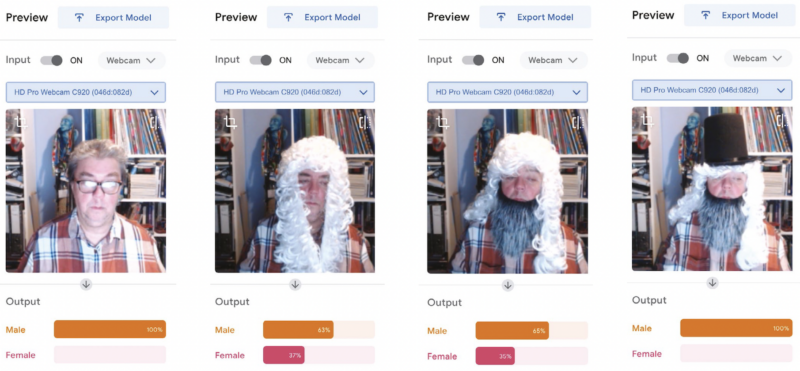
Once trained, try the model out. Props really help — a top hat, wig, and beard give the model a testing time (pun intended). In this test (see Figure 3), I presented myself to the model face-on and, unsurprisingly, I came out as 100 percent male. However, adding a judge’s wig forces the model into a rethink, and a beard produces a variety of results, but leaves the model unsure. It might be reasonable to assume that our model uses hair length as a strong feature. Adding a top hat to the ensemble brings the model back to a 100 percent prediction that the image is of a male.

Screenshots from Teachable Machine showing two datasets of a model classifying photos of the same face as either male or female with different degrees of confidence, based on the face is wearing a wig, a fake beard, or a tophat.
Figure 3: Outputs of a Teachable Machine model classifying photos of the author’s face as male or female with different degrees of confidence. Click to enlarge.

Machine learning uses a best-fit principle. The outputs, in this case whether I am male or female, have a greater certainty of male (65 percent) versus a lesser certainty of female (35 percent) if I wear a beard (Figure 3, second image from the right). Remove the beard and the likelihood of me being female increases by 2 percent (Figure 3, second image from the left).

Bias in machine learning models

Within a fairly small set of parameters, most human faces are similar. However, when you start digging, the research points to there being bias in AI (whether this is conscious or unconscious is a debate for another day!). You can exemplify this by firstly creating classes with labels such as ‘young smart’, ‘old smart’, ‘young not smart’, and ‘old not smart’. Select images that you think would fit the classes, and train them in Teachable Machine. You can then test the model by asking your students to find images they think fit each category. Run them against the model and ask students to debate whether the AI is acting fairly, and if not, why they think that is. Who is training these models? What images are they receiving? Similarly, you could create classes of images of known past criminals and heroes. Train the model before putting yourself in front of it. How far up the percentage scale are you towards being a criminal? It soon becomes frighteningly worrying that unless you are white and seemingly middle class, AI may prove problematic to you, from decisions on financial products such as mortgages through to mistaken arrest and identification.

It soon becomes frighteningly worrying that unless you are white and seemingly middle class, AI may prove problematic to you, from decisions on financial products such as mortgages through to mistaken arrest and identification.

Michael Jones

Encourage your students to discuss how they could influence this issue of race, class, and gender bias — for example, what rules would they use for identifying suitable images for a data set? There are some interesting articles on this issue that you can share with your students at helloworld.cc/aibias1 and helloworld.cc/aibias2.

Where next with your learners?

In the classroom, you could then follow the route of building models that identify letters for words, for example. One of my students built a model that could identify a range of spoons and forks. You may notice that Teachable Machine can also be run on Arduino boards, which adds an extra dimension. Why not get your students to create their own AI assistant that responds to commands? The possibilities are there to be explored. If you’re using webcams to collect photos yourself, why not create a system that will identify students? If you are lucky enough to have a set of identical twins in your class, that adds just a little more flavour! Teachable Machine offers a hands-on way to demonstrate the issues of AI accuracy and bias, and gives students a healthy opportunity for debate.

Michael Jones is director of Computer Science at Northfleet Technology College in the UK. He is a Specialist Leader of Education and a CS Champion for the National Centre for Computing Education.

More resources for AI and data science education

At the Foundation, AI education is one of our focus areas. Here is how we are supporting you and your learners in this area already:

  • Hello World issue 12 focuses on AI and machine learning education, with many practical resources, insightful interviews, and inspiring features from computer science educators. Download your free copy of issue 12 now.
  • In Hello World issue 16, the focus is on all things data science and data literacy for your learners. As always, you can download a free copy of the issue.
  • On our Hello World podcast, we’ve got episodes where we talk with practicing computing educators about how they bring AI, AI ethics, machine learning, and data science to the young people they teach.
  • If you’d like a practical introduction to the basics of machine learning and how to use it, take our free online course.
An image demonstrating that AI systems for object recognition do not distinguish between a real banana on a desk and the photo of a banana on a laptop screen.
  • Computing education researchers are working to answer the many open questions about what good AI and data science education looks like for young people. To learn more, you can watch the recordings from our research seminar series focused on this. We ourselves are working on research projects in this area and will share the results freely with the computing education community.
  • You can find a list of free educational resources about these topics that we’ve collated based on our research seminars, seminar participants’ recommendations, and our own work.

The post Classroom activities to discuss machine learning accuracy and ethics | Hello World #18 appeared first on Raspberry Pi.

AWS Week In Review – July 25, 2022

Post Syndicated from Antje Barth original https://aws.amazon.com/blogs/aws/aws-week-in-review-july-25-2022/

A few weeks ago, we hosted the first EMEA AWS Heroes Summit in Milan, Italy. This past week, I had the privilege to join the Americas AWS Heroes Summit in Seattle, Washington, USA. Meeting with our community experts is always inspiring and a great opportunity to learn from each other. During the Summit, AWS Heroes from North America and Latin America shared their thoughts with AWS developer advocates and product teams on topics such as serverless, containers, machine learning, data, and DevTools. You can learn more about the AWS Heroes program here.

AWS Heroes Summit Americas 2022

Last Week’s Launches
Here are some launches that got my attention during the previous week:

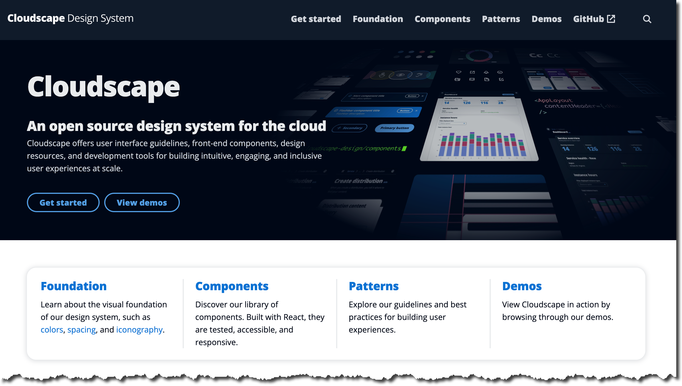
Cloudscape Design System Cloudscape is an open source design system for creating web applications. It was built for and is used by AWS products and services. We created it in 2016 to improve the user experience across web applications owned by AWS services and also to help teams implement those applications faster. If you’ve ever used the AWS Management Console, you’ve seen Cloudscape in action. If you are building a product that extends the AWS Management Console, designing a user interface for a hybrid cloud management system, or setting up an on-premises solution that uses AWS, have a look at Cloudscape Design System.

Cloudscape Design System

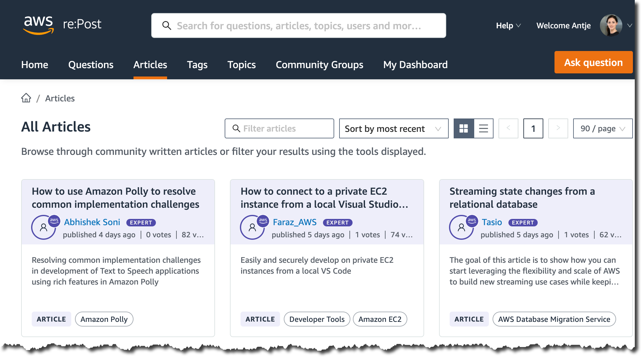
AWS re:Post introduces community-generated articlesAWS re:Post gives you access to a vibrant community that helps you become even more successful on AWS. Expert community members can now share technical guidance and knowledge beyond answering questions through the Articles feature. Using this feature, community members can share best practices and troubleshooting processes and address customer needs around AWS technology in greater depth. The Articles feature is unlocked for community members who have achieved Rising Star status on re:Post or subject matter experts who built their reputation in the community based on their contributions and certifications. If you have a Rising Star status on re:Post, start writing articles now! All other members can unlock Rising Star status through community contributions or simply browse available articles today on re:Post.

AWS re:Post

AWS Lambda announces support for attribute-based access control (ABAC) and new IAM condition key – You can now use attribute-based access control (ABAC) with AWS Lambda to control access to functions within AWS Identity and Access Management (IAM) using tags. ABAC is an authorization strategy that defines access permissions based on attributes. In AWS, these attributes are called tags. With ABAC, you can scale an access control strategy by setting granular permissions with tags without requiring permissions updates for every new user or resource as your organization scales. Read this blog post by Julian Wood and Chris McPeek to learn more.

AWS Lambda also announced support for lambda:SourceFunctionArn, a new IAM condition key that can be used for IAM policy conditions that specify the Amazon Resource Name (ARN) of the function from which a request is made. You can use the Condition element in your IAM policy to compare the lambda:SourceFunctionArn condition key in the request context with values that you specify in your policy. This allows you to implement advanced security controls for the AWS API calls taken by your Lambda function code. For more details, have a look at the Lambda Developer Guide.

Amazon Fraud Detector launches Account Takeover Insights (ATI)Amazon Fraud Detector now supports an Account Takeover Insights (ATI) model, a low-latency fraud detection machine learning model specifically designed to detect accounts that have been compromised through stolen credentials, phishing, social engineering, or other forms of account takeover. The ATI model is designed to detect up to four times more ATI fraud than traditional rules-based account takeover solutions while minimizing the level of friction for legitimate users. To learn more, have a look at the Amazon Fraud Detector documentation.

Amazon EMR on EC2 clusters (EMR Clusters) introduces more fine-grained access controls – Previously, all jobs running on an EMR cluster used the IAM role associated with the EMR cluster’s EC2 instances to access resources. This role is called the EMR EC2 instance profile. With the new runtime roles for Amazon EMR Steps, you can now specify a different IAM role for your Apache Spark and Hive jobs, scoping down access at a job level. This simplifies access controls on a single EMR cluster that is shared between multiple tenants, wherein each tenant is isolated using IAM roles. You can now also enforce table and column permissions based on your Amazon EMR runtime role to manage your access to data lakes with AWS Lake Formation. For more details, read the What’s New post.

For a full list of AWS announcements, be sure to keep an eye on the What’s New at AWS page.

Other AWS News
Here are some additional news and customer stories you may find interesting:

AWS open-source news and updates – My colleague Ricardo Sueiras writes this weekly open-source newsletter in which he highlights new open-source projects, tools, and demos from the AWS Community. Read edition #121 here.

AI Use Case Explorer – If you are interested in AI use cases, have a look at the new AI Use Case Explorer. You can search over 100 use cases and 400 customer success stories by industry, business function, and the business outcome you want to achieve.

Bayer centralizes and standardizes data from the carbon program using AWS – To help Brazilian farmers adopt climate-smart agricultural practices and reduce carbon emissions in their activities, Bayer created the Carbon Program, which aims to build carbon-neutral agriculture practices. Learn how Bayer uses AWS to centralize and standardize the data received from the different partners involved in the project in this Bayer case study.

Upcoming AWS Events
Check your calendars and sign up for these AWS events:

AWS re:Inforce 2022 – The event will be held this week in person on July 26 and 27 in Boston, Massachusetts, USA. You can watch the keynote and leadership sessions online for free. AWS On Air will also stream live from re:Inforce.

AWS SummitAWS Global Summits – AWS Global Summits are free events that bring the cloud computing community together to connect, collaborate, and learn about AWS. Registrations are open for the following AWS Summits in August:

Imagine Conference 2022IMAGINE 2022 – The IMAGINE 2022 conference will take place on August 3 at the Seattle Convention Center, Washington, USA. It’s a no-cost event that brings together education, state, and local leaders to learn about the latest innovations and best practices in the cloud. You can register here.
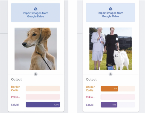
I’ll be speaking at Data Con LA on August 13–14 in Los Angeles, California, USA. Feel free to say “Hi!” if you’re around. And if you happen to be at Ray Summit on August 23–24 in San Francisco, California, USA, stop by the AWS booth. I’ll be there to discuss all things Ray on AWS.

That’s all for this week. Check back next Monday for another Week in Review!

Antje

This post is part of our Week in Review series. Check back each week for a quick roundup of interesting news and announcements from AWS!

New – Amazon SageMaker Ground Truth Now Supports Synthetic Data Generation

Post Syndicated from Antje Barth original https://aws.amazon.com/blogs/aws/new-amazon-sagemaker-ground-truth-now-supports-synthetic-data-generation/

Today, I am happy to announce that you can now use Amazon SageMaker Ground Truth to generate labeled synthetic image data.

Building machine learning (ML) models is an iterative process that, at a high level, starts with data collection and preparation, followed by model training and model deployment. And especially the first step, collecting large, diverse, and accurately labeled datasets for your model training, is often challenging and time-consuming.

Let’s take computer vision (CV) applications as an example. CV applications have come to play a key role in the industrial landscape. They help improve manufacturing quality or automate warehouses. Yet, collecting the data to train these CV models often takes a long time or can be impossible.

As a data scientist, you might spend months collecting hundreds of thousands of images from the production environments to make sure you capture all variations in data the model will come across. In some cases, finding all data variations might even be impossible, for example, sourcing images of rare product defects, or expensive, if you have to intentionally damage your products to get those images.

And once all data is collected, you need to accurately label the images, which is often a struggle in itself. Manually labeling images is slow and open to human error, and building custom labeling tools and setting up scaled labeling operations can be time-consuming and expensive. One way to mitigate this data challenge is by adding synthetic data to the mix.

Advantages of Combining Real-World Data with Synthetic Data
Combining your real-world data with synthetic data helps to create more complete training datasets for training your ML models.

Synthetic data itself is created by simple rules, statistical models, computer simulations, or other techniques. This allows synthetic data to be created in enormous quantities and with highly accurate labels for annotations across thousands of images. The label accuracy can be done at a very fine granularity, such as on a sub-object or pixel level, and across modalities. Modalities include bounding boxes, polygons, depth, and segments. Synthetic data can also be generated for a fraction of the cost, especially when compared to remote sensing imagery that otherwise relies on satellite, aerial, or drone image collection.

If you combine your real-world data with synthetic data, you can create more complete and balanced data sets, adding data variety that real-world data might lack. With synthetic data, you have the freedom to create any imagery environment, including edge cases that might be difficult to find and replicate in real-world data. You can customize objects and environments with variations, for example, to reflect different lighting, colors, texture, pose, or background. In other words, you can “order” the exact use case you are training your ML model for.

Now, let me show you how you can start sourcing labeled synthetic images using SageMaker Ground Truth.

Get Started on Your Synthetic Data Project with Amazon SageMaker Ground Truth
To request a new synthetic data project, navigate to the Amazon SageMaker Ground Truth console and select Synthetic data.

Amazon SageMaker Ground Truth Synthetic Data

Then, select Open project portal. In the project portal, you can request new projects, monitor projects that are in progress, and view batches of generated images once they become available for review. To initiate a new project, select Request project.

Amazon SageMaker Ground Truth Synthetic Data Project Portal

Describe your synthetic data needs and provide contact information.

Request a synthetic data project

After you submit the request form, you can check your project status in the project dashboard.

Amazon SageMaker Ground Truth Synthetic Data Project Created

In the next step, an AWS expert will reach out to discuss your project requirements in more detail. Upon review, the team will share a custom quote and project timeline.

If you want to continue, AWS digital artists will start by creating a small test batch of labeled synthetic images as a pilot production for you to review.

They collect your project inputs, such as reference photos and available 2D and 3D assets. The team then customizes those assets, adds the specified inclusions, such as scratches, dents, and textures, and creates the configuration that describes all the variations that need to be generated.

They can also create and add new objects based on your requirements, configure distributions and locations of objects in a scene, as well as modify object size, shape, color, and surface texture.

Once the objects are prepared, they are rendered using a photorealistic physics engine, capturing an image of the scene from a sensor that is placed in the virtual world. Images are also automatically labeled. Labels include 2D bounding boxes, instance segmentation, and contours.

You can monitor the progress of the data generation jobs on the project detail page. Once the pilot production test batch becomes available for review, you can spot-check the images and provide feedback for any rework that might be required.

Review available batches of synthetic data

Select the batch you want to review and View details
Sample batch of synthetic data in Amazon SageMaker Ground Truth

In addition to the images, you will also receive output image labels, metadata such as object positions, and image quality metrics as Amazon SageMaker compatible JSON files.

Synthetic Image Fidelity and Diversity Report
With each available batch of images, you also receive a synthetic image fidelity and diversity report. This report provides image and object level statistics and plots that help you make sense of the generated synthetic images.

The statistics are used to describe the diversity and the fidelity of the synthetic images and compare them with real images. Examples of the statistics and plots provided are the distributions of object classes, object sizes, image brightness, and image contrast, as well as the plots evaluating the indistinguishability between synthetic and real images.

Synthetic Image Fidelity and Diversity Report

Once you approve the pilot production test batch, the team will move to the production phase and start generating larger batches of labeled synthetic images with your desired label types, such as 2D bounding boxes, instance segmentation, and contours. Similar to the test batch, each production batch of images will be made available for you together with the image fidelity and diversity report to spot-check, accept, or reject.

All images and artifacts will be available for you to download from your S3 bucket once final production is complete.

Availability
Amazon SageMaker Ground Truth synthetic data is available in US East (N. Virginia). Synthetic data is priced on a per-label basis. You can request a custom quote that is tailored to your specific use case and requirements by filling out the project requirement form.

Learn more about SageMaker Ground Truth synthetic data on our Amazon SageMaker Data Labeling page.

Request your synthetic data project through the Amazon SageMaker Ground Truth console today!

— Antje

AWS Week In Review – June 6, 2022

Post Syndicated from Antje Barth original https://aws.amazon.com/blogs/aws/aws-week-in-review-june-6-2022/

This post is part of our Week in Review series. Check back each week for a quick roundup of interesting news and announcements from AWS!

I’ve just come back from a long (extended) holiday weekend here in the US and I’m still catching up on all the AWS launches that happened this past week. I’m particularly excited about some of the data, machine learning, and quantum computing news. Let’s have a look!

Last Week’s Launches
The launches that caught my attention last week are the following:

Amazon EMR Serverless is now generally available Amazon EMR Serverless allows you to run big data applications using open-source frameworks such as Apache Spark and Apache Hive without configuring, managing, and scaling clusters. The new serverless deployment option for Amazon EMR automatically scales resources up and down to provide just the right amount of capacity for your application, and you only pay for what you use. To learn more, check out Channy’s blog post and listen to The Official AWS Podcast episode on EMR Serverless.

AWS PrivateLink is now supported by additional AWS services AWS PrivateLink provides private connectivity between your virtual private cloud (VPC), AWS services, and your on-premises networks without exposing your traffic to the public internet. The following AWS services just added support for PrivateLink:

  • Amazon S3 on Outposts has added support for PrivateLink to perform management operations on your S3 storage by using private IP addresses in your VPC. This eliminates the need to use public IPs or proxy servers. Read the June 1 What’s New post for more information.
  • AWS Panorama now supports PrivateLink, allowing you to access AWS Panorama from your VPC without using public endpoints. AWS Panorama is a machine learning appliance and software development kit (SDK) that allows you to add computer vision (CV) to your on-premises cameras. Read the June 2 What’s New post for more information.
  • AWS Backup has added PrivateLink support for VMware workloads, providing direct access to AWS Backup from your VMware environment via a private endpoint within your VPC. Read the June 3 What’s New post for more information.

Amazon SageMaker JumpStart now supports incremental model training and automatic tuning – Besides ready-to-deploy solution templates for common machine learning (ML) use cases, SageMaker JumpStart also provides access to more than 300 pre-trained, open-source ML models. You can now incrementally train all the JumpStart models with new data without training from scratch. Through this fine-tuning process, you can shorten the training time to reach a better model. SageMaker JumpStart now also supports model tuning with SageMaker Automatic Model Tuning from its pre-trained model, solution templates, and example notebooks. Automatic tuning allows you to automatically search for the best hyperparameter configuration for your model.

Amazon Transcribe now supports automatic language identification for multi-lingual audioAmazon Transcribe converts audio input into text using automatic speech recognition (ASR) technology. If your audio recording contains more than one language, you can now enable multi-language identification, which identifies all languages spoken in the audio file and creates a transcript using each identified language. Automatic language identification for multilingual audio is supported for all 37 languages that are currently supported for batch transcriptions. Read the What’s New post from Amazon Transcribe to learn more.

Amazon Braket adds support for Borealis, the first publicly accessible quantum computer that is claimed to offer quantum advantage – If you are interested in quantum computing, you’ve likely heard the term “quantum advantage.” It refers to the technical milestone when a quantum computer outperforms the world’s fastest supercomputers on a well-defined task. Until now, none of the devices claimed to demonstrate quantum advantage have been accessible to the public. The Borealis device, a new photonic quantum processing unit (QPU) from Xanadu, is the first publicly available quantum computer that is claimed to have achieved quantum advantage. Amazon Braket, the quantum computing service from AWS, has just added support for Borealis. To learn more about how you can test a quantum advantage claim for yourself now on Amazon Braket, check out the What’s New post covering the addition of Borealis support.

For a full list of AWS announcements, be sure to keep an eye on the What’s New at AWS page.

Other AWS News
Some other updates and news that you may have missed:

New AWS Heroes – A warm welcome to our newest AWS Heroes! The AWS Heroes program is a worldwide initiative that acknowledges individuals who have truly gone above and beyond to share knowledge in technical communities. Get to know them in the June 2022 introduction blog post!

AWS open-source news and updates – My colleague Ricardo Sueiras writes this weekly open-source newsletter in which he highlights new open-source projects, tools, and demos from the AWS Community. Read edition #115 here.

Upcoming AWS Events
Join me in Las Vegas for Amazon re:MARS 2022. The conference takes place June 21–24 and is all about the latest innovations in machine learning, automation, robotics, and space. I will deliver a talk on how machine learning can help to improve disaster response. Say “Hi!” if you happen to be around and see me.

We also have more AWS Summits coming up over the next couple of months, both in-person and virtual.

In Europe:

In North America:

In South America:

Find an AWS Summit near you, and get notified when registration opens in your area.

Imagine Conference 2022You can now register for IMAGINE 2022 (August 3, Seattle). The IMAGINE 2022 conference is a no-cost event that brings together education, state, and local leaders to learn about the latest innovations and best practices in the cloud.

Sign up for the SQL Server Database Modernization webinar on June 21 to learn how to modernize and cost-optimize Microsoft SQL Server on AWS.

That’s all for this week. Check back next Monday for another Week in Review!

— Antje

Use a linear learner algorithm in Amazon Redshift ML to solve regression and classification problems

Post Syndicated from Phil Bates original https://aws.amazon.com/blogs/big-data/use-a-linear-learner-algorithm-in-amazon-redshift-ml-to-solve-regression-and-classification-problems/

Amazon Redshift is the fastest, most widely used, fully managed, and petabyte-scale cloud data warehouse. Tens of thousands of customers use Amazon Redshift to process exabytes of data every day to power their analytics workloads. Amazon Redshift ML, powered by Amazon SageMaker, makes it easy for SQL users such as data analysts, data scientists, and database developers to create, train, and deploy machine learning (ML) models using familiar SQL commands and then use these models to make predictions on new data for use cases such as churn prediction, customer lifetime value prediction, and product recommendations. Redshift ML makes the model available as a SQL function within the Amazon Redshift data warehouse so you can easily use it in queries and reports. Customers across all verticals are using Redshift ML to derive better insights from their data. For example, Jobcase uses Redshift ML to recommend job search at scale. Magellan RX Management uses Redshift ML to predict drug therapeutic use conditions.

Amazon Redshift supports supervised learning, including regression, binary classification, multi-class classification, and unsupervised learning using K-Means. You can optionally specify XGBoost, MLP, and now linear learner model types, which are supervised learning algorithms used for solving either classification or regression problems, and provide a significant increase in speed over traditional hyperparameter optimization techniques. Amazon Redshift also supports bring-your-own-model to invoke remote SageMaker endpoints.

In this post, we show you how to use Redshift ML to solve regression and classification problems using the SageMaker linear learner algorithm, which explores different training objectives and chooses the best solution from a validation set.

Solution overview

We first solve a linear regression problem, followed by a multi-class classification problem.

The following table shows some common use cases and algorithms used.

Use Case Algorithm / Problem Type
Customer churn prediction Classification
Predict if a sales lead will close Classification
Fraud detection Classification
Price and revenue prediction Linear regression
Customer lifetime value prediction Linear regression

To use the linear learner algorithm, you need to provide inputs or columns representing dimensional values and also the label or target, which is the value you’re trying to predict. The linear learner algorithm trains many models in parallel, and automatically determines the most optimized model.

Prerequisites

To get started, we need an Amazon Redshift cluster or an Amazon Redshift Serverless endpoint and an AWS Identity and Access Management (IAM) role attached that provides access to SageMaker and permissions to an Amazon Simple Storage Service (Amazon S3) bucket.

For an introduction to Redshift ML and instructions on setting it up, see Create, train, and deploy machine learning models in Amazon Redshift using SQL with Amazon Redshift ML.

To create a simple cluster with a default IAM role, see Use the default IAM role in Amazon Redshift to simplify accessing other AWS services.

Use case 1: Linear regression

In this use case, we analyze the Abalone dataset and determine the relationship between the physical measurements and use that to determine the age of abalone. The age of abalone is determined by cutting the shell through the cone, staining it, and counting the number of rings through a microscope, which is a time-consuming task. We want to predict the age using different physical measurements, which is easier to measure. The age of abalone is (number of rings + 1.5) years.

Prepare the data

Load the Abalone dataset into Amazon Redshift using the following SQL. You can use the Amazon Redshift query editor v2 or your preferred SQL tool to run these commands.

To create the table, use the following commands:

create table abalone_dataset
( 
id INT IDENTITY(1,1),
Sex     CHAR(1),
Length float,
Diameter float,
Height float,
Whole  float,
Shucked  float,
Viscera  float,
Shell float,
Rings  integer   
); 

To load data into Amazon Redshift, use the following COPY command:

COPY abalone_dataset 
from 's3://redshift-ml-multiclass/abalone.csv' 
REGION 'us-east-1'
IAM_ROLE default
CSV IGNOREHEADER 1
NULL AS 'NULL'; 

To train the model, we use the abalone table and 80% of the data to train the model, and then test the accuracy of that model by seeing if it correctly predicts the age of ring label attribute on the remaining 20% of the data. Run the following command to create training and validation tables:

create table abalone_training as
  select * from abalone_dataset where mod(id,10) < 8 ; 

create table abalone_validation as
  select * from abalone_dataset where mod(id,10) >= 8; 

Create a model in Redshift ML

To create a model in Amazon Redshift, use the following command:

CREATE MODEL model_abalone_ring_prediction
FROM (
 SELECT   Sex ,
Length ,
Diameter ,
Height ,
Whole  ,
Shucked  ,
Viscera  ,
Shell,
Rings  as target_label
FROM abalone_training
) TARGET target_label
FUNCTION f_abalone_ring_prediction
IAM_ROLE default
MODEL_TYPE LINEAR_LEARNER 
PROBLEM_TYPE REGRESSION
OBJECTIVE 'MSE'
SETTINGS (
  S3_BUCKET '<your-s3-bucket>',
  MAX_RUNTIME 15000
  ); 

We define the following parameters in the CREATE MODEL statement:

  • Problem type – We use the linear learner problem type, which is newly added to extend upon typical linear models by training many models in parallel, in a computationally efficient manner.
  • Objective – We specified MSE (mean square error) as our objective, which is a common metric for evaluation of regression problems.
  • Max runtime –This parameter denotes how long the model training can run. Specifying a larger value may help create a better tuned model. The default value for this parameter is 5400 (90 minutes). For this example, we set it to 15000.

The preceding statement takes a few seconds to complete. It initiates an Amazon SageMaker Autopilot process in the background to automatically build, train, and tune the best ML model for the input data. It then uses Amazon SageMaker Neo to deploy that model locally in the Amazon Redshift cluster or Amazon Redshift Serverless as a user-defined function (UDF). You can use the SHOW MODEL command in Amazon Redshift to track the progress of your model creation, which should be in the READY state within the max_runtime parameter you defined while creating the model.

To check the status of the model, use the following command:

show model model_abalone_ring_prediction;

The following is the tabular outcome for the preceding command after model training was done. It took approximately 120 minutes to train the model.

Key Value
Model Name model_abalone_ring_prediction
Schema Name public
Owner awsuser
Creation Time Tue, 10.05.2022 19:42:33
Model State READY
validation:mse 4.082088
Estimated Cost 5.423719
. .
TRAINING DATA: .
Query SELECT SEX , LENGTH , DIAMETER , HEIGHT , WHOLE , SHUCKED , VISCERA , SHELL, RINGS AS TARGET_LABEL
. FROM ABALONE_TRAINING
Target Column TARGET_LABEL
. .
PARAMETERS: .
Model Type linear_learner
Problem Type Regression
Objective MSE
AutoML Job Name redshiftml-20220510194233380173
Function Name f_abalone_ring_prediction
Function Parameters sex length diameter height whole shucked viscera shell
Function Parameter Types bpchar float8 float8 float8 float8 float8 float8 float8
IAM Role default-aws-iam-role
S3 Bucket poc-generic-bkt
Max Runtime 15000

Model validation

We notice from the preceding table that the MSE for the training data is 4.08. Now let’s run the prediction query and validate the accuracy of the model on the testing and validation dataset:

select
ROUND(AVG(POWER(( tgt_label - predicted ),2)),2) mse
, ROUND(SQRT(AVG(POWER(( tgt_label - predicted ),2))),2) rmse
from 
(
SELECT   Sex ,
Length ,
Diameter ,
Height ,
Whole  ,
Shucked  ,
Viscera  ,
Shell,
Rings as tgt_label,
f_abalone_ring_prediction(Sex ,Length ,Diameter ,Height ,Whole  ,Shucked  ,Viscera  ,Shell) as predicted,
case when tgt_label = predicted then 1
      else 0 end as match,
  case when tgt_label  <> predicted then 1
    else 0 end as nonmatch
FROM abalone_validation
)t1 

The following is the outcome from the query:

mse rmse
5.08 2.25

The MSE value from the preceding query results indicates that our model is accurate enough to the actual values from our validation dataset.

We can also observe that Redshift ML is able to identify the right combination of features to come up with a usable prediction model. We can further check the impact of each attribute and its contribution and weightage in the model selection using the following command:

select explain_model ('model_abalone_ring_prediction')

The following is the outcome, where each attribute weightage is representative of its role in model decision-making:

{"explanations":
    {"kernel_shap":
      {"label0":
        {"expected_value":10.06938362121582,
          "global_shap_values":
          {
            "diameter":0.6897614190439705,
            "height":0.38391156156643987,
            "length":0.29646334630067408,
            "sex":0.5516722137411109,
            "shell":1.5679368167990147,
            "shucked":2.222549468867254,
            "viscera":0.2879883139361144,
            "whole":0.8085603201751219
            }
        }
       }
      }
      ,"version":"1.0"
    }

Use case 2: Multi-class classification

For this use case, we use the Covertype dataset (copyright Jock A. Blackard and Colorado State University), which contains information collected by the US Geological Survey and the US Forest Service about wilderness areas in northern Colorado. This has been downloaded to an S3 bucket to make it simple to create the model. You may want to download the dataset description. This dataset contains various measurements such as elevation, distance to waters and roadways, as well as the wilderness area designation and the soil type. Our ML task is to create a model to predict the cover type for a given area.

Prepare the data

To prepare the data for this model, you need to create and populate the table public.covertype_data in Amazon Redshift using the Covertype dataset. You may use the following SQL in Amazon Redshift query editor v2 or your preferred SQL tool:

CREATE TABLE public.covertype_data (
    elevation bigint ENCODE az64,
    aspect bigint ENCODE az64,
    slope bigint ENCODE az64,
    horizontal_distance_to_hydrology bigint ENCODE az64,
    vertical_distance_to_hydrology bigint ENCODE az64,
    horizontal_distance_to_roadways bigint ENCODE az64,
    hillshade_9am bigint ENCODE az64,
    hillshade_noon bigint ENCODE az64,
    hillshade_3pm bigint ENCODE az64,
    horizontal_distance_to_fire_points bigint ENCODE az64,
    wilderness_area1 bigint ENCODE az64,
    wilderness_area2 bigint ENCODE az64,
    wilderness_area3 bigint ENCODE az64,
    wilderness_area4 bigint ENCODE az64,
    soil_type1 bigint ENCODE az64,
    soil_type2 bigint ENCODE az64,
    soil_type3 bigint ENCODE az64,
    soil_type4 bigint ENCODE az64,
    soil_type5 bigint ENCODE az64,
    soil_type6 bigint ENCODE az64,
    soil_type7 bigint ENCODE az64,
    soil_type8 bigint ENCODE az64,
    soil_type9 bigint ENCODE az64,
    soil_type10 bigint ENCODE az64,
    soil_type11 bigint ENCODE az64,
    soil_type12 bigint ENCODE az64,
    soil_type13 bigint ENCODE az64,
    soil_type14 bigint ENCODE az64,
    soil_type15 bigint ENCODE az64,
    soil_type16 bigint ENCODE az64,
    soil_type17 bigint ENCODE az64,
    soil_type18 bigint ENCODE az64,
    soil_type19 bigint ENCODE az64,
    soil_type20 bigint ENCODE az64,
    soil_type21 bigint ENCODE az64,
    soil_type22 bigint ENCODE az64,
    soil_type23 bigint ENCODE az64,
    soil_type24 bigint ENCODE az64,
    soil_type25 bigint ENCODE az64,
    soil_type26 bigint ENCODE az64,
    soil_type27 bigint ENCODE az64,
    soil_type28 bigint ENCODE az64,
    soil_type29 bigint ENCODE az64,
    soil_type30 bigint ENCODE az64,
    soil_type31 bigint ENCODE az64,
    soil_type32 bigint ENCODE az64,
    soil_type33 bigint ENCODE az64,
    soil_type34 bigint ENCODE az64,
    soil_type35 bigint ENCODE az64,
    soil_type36 bigint ENCODE az64,
    soil_type37 bigint ENCODE az64,
    soil_type38 bigint ENCODE az64,
    soil_type39 bigint ENCODE az64,
    soil_type40 bigint ENCODE az64,
    cover_type bigint ENCODE az64 
)
DISTSTYLE AUTO;	


Copy public.covertype_data
From 's3://redshift-ml-multiclass/covtype.data.gz'
iam_role default 
gzip
delimiter ','
region 'us-east-1';

Now that our dataset is loaded, we run the following SQL statements to split the data into three sets for training (80%), validation (10%), and prediction (10%). Note that Redshift ML Autopilot automatically splits the data into training and validation, but by splitting it here, you’re able to verify the accuracy of your model.

To prepare the dataset, assign random values to split the data:

create table  public.covertype_data_prep  as
select a.*,
cast (random() * 80 as int) as data_group_id
from public.covertype_data a;

Use the following code for the training set:

Create table public.covertype_training as
Select * from public.covertype_data_prep
Where data_group_id < 80;

Use the following code for the validation set:

Create table public.covertype_validation as
Select * from public.covertype_data_prep
Where data_group_id between 80 and 89;

Use the following code for the test set:

Create table public.covertype_test as
Select * from public.covertype_data_prep
Where data_group_id > 89; 

Now that we have our datasets, it’s time to create the model.

Create a model in Redshift ML using linear learner

Run the following SQL command to create your model—note our target is cover_type and we use all the inputs from our training set:

CREATE  MODEL forest_cover_type_model
FROM (select Elevation, 
   Aspect,  
   Slope,  
   Horizontal_distance_to_hydrology,  
   Vertical_distance_to_hydrology,   
   Horizontal_distance_to_roadways,  
   HIllshade_9am,  
   Hillshade_noon,  
   Hillshade_3pm , 
   Horizontal_Distance_To_Fire_Points,  
   Wilderness_Area1,  
   Wilderness_Area2,   
   Wilderness_Area3,  
   Wilderness_Area4,  
   soil_type1,
   Soil_Type2,
   Soil_Type3, 
   Soil_Type4, 
   Soil_Type5,  
   Soil_Type6, 
   Soil_Type7,  
   Soil_Type8, 
   Soil_Type9, 
   Soil_Type10 , 
   Soil_Type11,  
   Soil_Type12 , 
   Soil_Type13 ,
   Soil_Type14, 
   Soil_Type15, 
   Soil_Type16,  
   Soil_Type17, 
   Soil_Type18,  
   Soil_Type19,  
   Soil_Type20,  
   Soil_Type21,  
   Soil_Type22,  
   Soil_Type23,  
   Soil_Type24, 
   Soil_Type25,  
   Soil_Type26, 
   Soil_Type27,  
   Soil_Type28,  
   Soil_Type29,  
   Soil_Type30,  
   Soil_Type31, 
   Soil_Type32, 
   Soil_Type33,  
   Soil_Type34, 
   Soil_Type36, 
   Soil_Type37,  
   Soil_Type38,  
   Soil_Type39, 
   Soil_Type40,
  Cover_type from public.covertype_training)
TARGET cover_type
FUNCTION predict_cover_type
IAM_ROLE default
MODEL_TYPE LINEAR_LEARNER              
PROBLEM_TYPE MULTICLASS_CLASSIFICATION 
 OBJECTIVE 'Accuracy'
SETTINGS (
  S3_BUCKET '<<your-amazon-s3-bucket-name>>’
, 
  S3_GARBAGE_COLLECT OFF,
  MAX_RUNTIME 9600
) ;

You can use the SHOW MODEL command to view the status of the model.

You can see that the model has an accuracy score of .730279 and is in the READY state. Now let’s run a query to do some validation of our own.

Model validation

Run the following SQL query against the validation table, using the function created by our model:

select 
 cast(sum(t1.match)as decimal(7,2)) as predicted_matches
,cast(sum(t1.nonmatch) as decimal(7,2)) as predicted_non_matches
,cast(sum(t1.match + t1.nonmatch) as decimal(7,2))  as total_predictions
,predicted_matches / total_predictions as pct_accuracy
from 
(select 
Elevation, 
   Aspect,  
   Slope,  
   Horizontal_distance_to_hydrology,  
   Vertical_distance_to_hydrology,   
   Horizontal_distance_to_roadways,  
   HIllshade_9am,  
   Hillshade_noon,  
   Hillshade_3pm , 
   Horizontal_Distance_To_Fire_Points,  
   Wilderness_Area1,  
   Wilderness_Area2,   
   Wilderness_Area3,  
   Wilderness_Area4,  
   soil_type1,
   Soil_Type2,
   Soil_Type3, 
   Soil_Type4, 
   Soil_Type5,  
   Soil_Type6, 
   Soil_Type7,  
   Soil_Type8, 
   Soil_Type9, 
   Soil_Type10 , 
   Soil_Type11,  
   Soil_Type12 , 
   Soil_Type13 ,
   Soil_Type14, 
   Soil_Type15, 
   Soil_Type16,  
   Soil_Type17, 
   Soil_Type18,  
   Soil_Type19,  
   Soil_Type20,  
   Soil_Type21,  
   Soil_Type22,  
   Soil_Type23,  
   Soil_Type24, 
   Soil_Type25,  
   Soil_Type26, 
   Soil_Type27,  
   Soil_Type28,  
   Soil_Type29,  
   Soil_Type30,  
   Soil_Type31, 
   Soil_Type32, 
   Soil_Type33,  
   Soil_Type34, 
   Soil_Type36, 
   Soil_Type37,  
   Soil_Type38,  
   Soil_Type39, 
   Soil_Type40,
   Cover_type as actual_cover_type,
   predict_cover_type( Elevation, 
   Aspect,  
   Slope,  
   Horizontal_distance_to_hydrology,  
   Vertical_distance_to_hydrology,   
   Horizontal_distance_to_roadways,  
   HIllshade_9am,  
   Hillshade_noon,  
   Hillshade_3pm , 
   Horizontal_Distance_To_Fire_Points,  
   Wilderness_Area1,  
   Wilderness_Area2,   
   Wilderness_Area3,  
   Wilderness_Area4,  
   soil_type1,
   Soil_Type2,
   Soil_Type3, 
   Soil_Type4, 
   Soil_Type5,  
   Soil_Type6, 
   Soil_Type7,  
   Soil_Type8, 
   Soil_Type9, 
   Soil_Type10 , 
   Soil_Type11,  
   Soil_Type12 , 
   Soil_Type13 ,
   Soil_Type14, 
   Soil_Type15, 
   Soil_Type16,  
   Soil_Type17, 
   Soil_Type18,  
   Soil_Type19,  
   Soil_Type20,  
   Soil_Type21,  
   Soil_Type22,  
   Soil_Type23,  
   Soil_Type24, 
   Soil_Type25,  
   Soil_Type26, 
   Soil_Type27,  
   Soil_Type28,  
   Soil_Type29,  
   Soil_Type30,  
   Soil_Type31, 
   Soil_Type32, 
   Soil_Type33,  
   Soil_Type34, 
   Soil_Type36, 
   Soil_Type37,  
   Soil_Type38,  
   Soil_Type39, 
   Soil_Type40) as predicted_cover_type,
case when actual_cover_type = predicted_cover_type then 1
      else 0 end as match,
  case when actual_cover_type <>  predicted_cover_type then 1
    else 0 end as nonmatch

from public.covertype_validation
) t1;

You can see that our accuracy is very close to our score from the SHOW MODEL output.

Run a prediction query

Let’s run a prediction query in Amazon Redshift ML using our function against our test dataset to see the most common class of cover type for the Neota Wilderness Area. We can denote this by checking wildnerness_area2 for a value of 1.

The dataset includes the following wilderness areas:

  1. Rawah Wilderness Area
  2. Neota Wilderness Area
  3. Comanche Peak Wilderness Area
  4. Cache la Poudre Wilderness Area

The cover types are in seven different classes:

  1. Spruce/Fir
  2. Lodgepole Pine
  3. Ponderosa Pine
  4. Cottonwood/Willow
  5. Aspen
  6. Douglas Fir
  7. Krummholz

There are also 40 different soil type definitions, which you can see in the dataset description, with a value of 0 or 1 to note if it’s applicable for a particular row. The following are a few example soil types:

  1. Cathedral family – Rock outcrop complex, extremely stony
  2. Vanet-Ratake families –Rocky outcrop complex, very stony
  3. Haploborolis family – Rock outcrop complex, rubbly
  4. Ratake family – Rock outcrop complex, rubbly
  5. Vanet family – Rock outcrop complex, rubbly
  6. Vanet-Wetmore families – Rock outcrop complex, stony
select t1. predicted_cover_type, count(*) 
from 
(     
select 
   Elevation, 
   Aspect,  
   Slope,  
   Horizontal_distance_to_hydrology,  
   Vertical_distance_to_hydrology,   
   Horizontal_distance_to_roadways,  
   HIllshade_9am,  
   Hillshade_noon,  
   Hillshade_3pm , 
   Horizontal_Distance_To_Fire_Points,  
   Wilderness_Area1,  
   Wilderness_Area2,   
   Wilderness_Area3,  
   Wilderness_Area4,  
   soil_type1,
   Soil_Type2,
   Soil_Type3, 
   Soil_Type4, 
   Soil_Type5,  
   Soil_Type6, 
   Soil_Type7,  
   Soil_Type8, 
   Soil_Type9, 
   Soil_Type10 , 
   Soil_Type11,  
   Soil_Type12 , 
   Soil_Type13 ,
   Soil_Type14, 
   Soil_Type15, 
   Soil_Type16,  
   Soil_Type17, 
   Soil_Type18,  
   Soil_Type19,  
   Soil_Type20,  
   Soil_Type21,  
   Soil_Type22,  
   Soil_Type23,  
   Soil_Type24, 
   Soil_Type25,  
   Soil_Type26, 
   Soil_Type27,  
   Soil_Type28,  
   Soil_Type29,  
   Soil_Type30,  
   Soil_Type31, 
   Soil_Type32, 
   Soil_Type33,  
   Soil_Type34, 
   Soil_Type36, 
   Soil_Type37,  
   Soil_Type38,  
   Soil_Type39, 
   Soil_Type40,
   predict_cover_type( Elevation, 
   Aspect,  
   Slope,  
   Horizontal_distance_to_hydrology,  
   Vertical_distance_to_hydrology,   
   Horizontal_distance_to_roadways,  
   HIllshade_9am,  
   Hillshade_noon,  
   Hillshade_3pm , 
   Horizontal_Distance_To_Fire_Points,  
   Wilderness_Area1,  
   Wilderness_Area2,   
   Wilderness_Area3,  
   Wilderness_Area4,  
   soil_type1,
   Soil_Type2,
   Soil_Type3, 
   Soil_Type4, 
   Soil_Type5,  
   Soil_Type6, 
   Soil_Type7,  
   Soil_Type8, 
   Soil_Type9, 
   Soil_Type10,
   Soil_Type11,  
   Soil_Type12, 
   Soil_Type13,
   Soil_Type14, 
   Soil_Type15, 
   Soil_Type16,  
   Soil_Type17, 
   Soil_Type18,  
   Soil_Type19,  
   Soil_Type20,  
   Soil_Type21,  
   Soil_Type22,  
   Soil_Type23,  
   Soil_Type24, 
   Soil_Type25,  
   Soil_Type26, 
   Soil_Type27,  
   Soil_Type28,  
   Soil_Type29,  
   Soil_Type30,  
   Soil_Type31, 
   Soil_Type32, 
   Soil_Type33,  
   Soil_Type34, 
   Soil_Type36, 
   Soil_Type37,  
   Soil_Type38,  
   Soil_Type39, 
   Soil_Type40) as predicted_cover_type 

from public.covertype_test
where wilderness_area2 = 1)
t1
group by 1;

Our model has predicted that the majority of cover is Spruce and Fir.

You can experiment with various combinations, such as determining which soil types are most likely to occur in a predicted cover type.

Conclusion

Redshift ML makes it easy for users of all levels to create, train, and tune models using a SQL interface. In this post, we walked you through how to use the linear learner algorithm to create regression and multi-class classification models. You can then use those models to make predictions using simple SQL commands and gain valuable insights.

To learn more about RedShift ML, visit Amazon Redshift ML.


About the Authors

Phil Bates is a Senior Analytics Specialist Solutions Architect at AWS with over 25 years of data warehouse experience.

Sohaib Katariwala is an Analytics Specialist Solutions Architect at AWS. He has 12+ years of experience helping organizations derive insights from their data.

Tahir Aziz is an Analytics Solution Architect at AWS. He has worked with building data warehouses and big data solutions for over 13 years. He loves to help customers design end-to-end analytics solutions on AWS. Outside of work, he enjoys traveling and cooking.

Jiayuan Chen is a Senior Software Development Engineer at AWS. He is passionate about designing and building data-intensive applications, and has been working in the areas of data lake, query engine, ingestion, and analytics. He keeps up with latest technologies and innovates things that spark joy.

Debu Panda is a Senior Manager, Product Management at AWS, is an industry leader in analytics, application platform, and database technologies, and has more than 25 years of experience in the IT world. Debu has published numerous articles on analytics, enterprise Java, and databases and has presented at multiple conferences such as re:Invent, Oracle Open World, and Java One. He is lead author of the EJB 3 in Action (Manning Publications 2007, 2014) and Middleware Management (Packt).

A new Spark plugin for CPU and memory profiling

Post Syndicated from Bo Xiong original https://aws.amazon.com/blogs/devops/a-new-spark-plugin-for-cpu-and-memory-profiling/

Introduction

Have you ever wondered if there are low-hanging optimization opportunities to improve the performance of a Spark app? Profiling can help you gain visibility regarding the runtime characteristics of the Spark app to identify its bottlenecks and inefficiencies. We’re excited to announce the release of a new Spark plugin that enables profiling for JVM based Spark apps via Amazon CodeGuru. The plugin is open sourced on GitHub and published to Maven.

Walkthrough

This post shows how you can onboard this plugin with two steps in under 10 minutes.

  • Step 1: Create a profiling group in Amazon CodeGuru Profiler and grant permission to your Amazon EMR on EC2 role, so that profiler agents can emit metrics to CodeGuru. Detailed instructions can be found here.
  • Step 2: Reference codeguru-profiler-for-spark when submitting your Spark job, along with PROFILING_CONTEXT and ENABLE_AMAZON_PROFILER defined.

Prerequisites

Your app is built against Spark 3 and run on Amazon EMR release 6.x or newer. It doesn’t matter if you’re using Amazon EMR on Amazon Elastic Compute Cloud (Amazon EC2) or on Amazon Elastic Kubernetes Service (Amazon EKS).

Illustrative Example

For the purposes of illustration, consider the following example where profiling results are collected by the plugin and emitted to the “CodeGuru-Spark-Demo” profiling group.

spark-submit \
--master yarn \
--deploy-mode cluster \
--class \
--packages software.amazon.profiler:codeguru-profiler-for-spark:1.0 \
--conf spark.plugins=software.amazon.profiler.AmazonProfilerPlugin \
--conf spark.executorEnv.PROFILING_CONTEXT="{\\\"profilingGroupName\\\":\\\"CodeGuru-Spark-Demo\\\"}" \
--conf spark.executorEnv.ENABLE_AMAZON_PROFILER=true \
--conf spark.dynamicAllocation.enabled=false \t

An alternative way to specify PROFILING_CONTEXT and ENABLE_AMAZON_PROFILER is under the yarn-env.export classification for instance groups in the Amazon EMR web console. Note that PROFILING_CONTEXT, if configured in the web console, must escape all of the commas on top of what’s for the above spark-submit command.

[
  {
    "classification": "yarn-env",
    "properties": {},
    "configurations": [
      {
        "classification": "export",
        "properties": {
          "ENABLE_AMAZON_PROFILER": "true",
          "PROFILING_CONTEXT": "{\\\"profilingGroupName\\\":\\\"CodeGuru-Spark-Demo\\\"\\,\\\"driverEnabled\\\":\\\"true\\\"}"
        },
        "configurations": []
      }
    ]
  }
]

Once the job above is launched on Amazon EMR, profiling results should show up in your CodeGuru web console in about 10 minutes, similar to the following screenshot. Internally, it has helped us identify issues, such as thread contentions (revealed by the BLOCKED state in the latency flame graph), and unnecessarily create AWS Java clients (revealed by the CPU Hotspots view).

Go to your profiling group under the Amazon CodeGuru web console. Click the “Visualize CPU” button to render a flame graph displaying CPU usage. Switch to the latency view to identify latency bottlenecks, and switch to the heap summary view to identify objects consuming most memory.

Troubleshooting

To help with troubleshooting, use a sample Spark app provided in the plugin to check if everything is set up correctly. Note that the profilingGroupName value specified in PROFILING_CONTEXT should match what’s created in CodeGuru.

spark-submit \
--master yarn \
--deploy-mode cluster \
--class software.amazon.profiler.SampleSparkApp \
--packages software.amazon.profiler:codeguru-profiler-for-spark:1.0 \
--conf spark.plugins=software.amazon.profiler.AmazonProfilerPlugin \
--conf spark.executorEnv.PROFILING_CONTEXT="{\\\"profilingGroupName\\\":\\\"CodeGuru-Spark-Demo\\\"}" \
--conf spark.executorEnv.ENABLE_AMAZON_PROFILER=true \
--conf spark.yarn.appMasterEnv.PROFILING_CONTEXT="{\\\"profilingGroupName\\\":\\\"CodeGuru-Spark-Demo\\\",\\\"driverEnabled\\\":\\\"true\\\"}" \
--conf spark.yarn.appMasterEnv.ENABLE_AMAZON_PROFILER=true \
--conf spark.dynamicAllocation.enabled=false \
/usr/lib/hadoop-yarn/hadoop-yarn-server-tests.jar

Running the command above from the master node of your EMR cluster should produce logs similar to the following:

21/11/21 21:27:21 INFO Profiler: Starting the profiler : ProfilerParameters{profilingGroupName='CodeGuru-Spark-Demo', threadSupport=BasicThreadSupport (default), excludedThreads=[Signal Dispatcher, Attach Listener], shouldProfile=true, integrationMode='', memoryUsageLimit=104857600, heapSummaryEnabled=true, stackDepthLimit=1000, samplingInterval=PT1S, reportingInterval=PT5M, addProfilerOverheadAsSamples=true, minimumTimeForReporting=PT1M, dontReportIfSampledLessThanTimes=1}
21/11/21 21:27:21 INFO ProfilingCommandExecutor: Profiling scheduled, sampling rate is PT1S
...
21/11/21 21:27:23 INFO ProfilingCommand: New agent configuration received : AgentConfiguration(AgentParameters={MaxStackDepth=1000, MinimumTimeForReportingInMilliseconds=60000, SamplingIntervalInMilliseconds=1000, MemoryUsageLimitPercent=10, ReportingIntervalInMilliseconds=300000}, PeriodInSeconds=300, ShouldProfile=true)
21/11/21 21:32:23 INFO ProfilingCommand: Attempting to report profile data: start=2021-11-21T21:27:23.227Z end=2021-11-21T21:32:22.765Z force=false memoryRefresh=false numberOfTimesSampled=300
21/11/21 21:32:23 INFO javaClass: [HeapSummary] Processed 20 events.
21/11/21 21:32:24 INFO ProfilingCommand: Successfully reported profile

Note that the CodeGuru Profiler agent uses a reporting interval of five minutes. Therefore, any executor process shorter than five minutes won’t be reflected by the profiling result. If the right profiling group is not specified, or it’s associated with a wrong EC2 role in CodeGuru, then the log will show a message similar to “CodeGuruProfilerSDKClient: Exception while calling agent orchestration” along with a stack trace including a 403 status code. To rule out any network issues (e.g., your EMR job running in a VPC without an outbound gateway or a misconfigured outbound security group), then you can remote into an EMR host and ping the CodeGuru endpoint in your Region (e.g., ping codeguru-profiler.us-east-1.amazonaws.com).

Cleaning up

To avoid incurring future charges, you can delete the profiling group configured in CodeGuru and/or set the ENABLE_AMAZON_PROFILER environment variable to false.

Conclusion

In this post, we describe how to onboard this plugin with two steps. Consider to give it a try for your Spark app? You can find the Maven artifacts here. If you have feature requests, bug reports, feedback of any kind, or would like to contribute, please head over to the GitHub repository.

Author:

Bo Xiong

Bo Xiong is a software engineer with Amazon Ads, leveraging big data technologies to process petabytes of data for billing and reporting. His main interests include performance tuning and optimization for Spark on Amazon EMR, and data mining for actionable business insights.

Optimize AI/ML workloads for sustainability: Part 3, deployment and monitoring

Post Syndicated from Benoit de Chateauvieux original https://aws.amazon.com/blogs/architecture/optimize-ai-ml-workloads-for-sustainability-part-3-deployment-and-monitoring/

We’re celebrating Earth Day 2022 from 4/22 through 4/29 with posts that highlight how to build, maintain, and refine your workloads for sustainability.


AWS estimates that inference (the process of using a trained machine learning [ML] algorithm to make a prediction) makes up 90 percent of the cost of an ML model. Given with AWS you pay for what you use, we estimate that inference also generally equates to most of the resource usage within an ML lifecycle.

In this series, we’re following the phases of the Well-Architected machine learning lifecycle (Figure 1) to optimize your artificial intelligence (AI)/ML workloads. In Part 3, our final piece in the series, we show you how to reduce the environmental impact of your ML workload once your model is in production.


If you missed the first parts of this series, in Part 1, we showed you how to examine your workload to help you 1) evaluate the impact of your workload, 2) identify alternatives to training your own model, and 3) optimize data processing. In Part 2, we identified ways to reduce the environmental impact of developing, training, and tuning ML models.


ML lifecycle

Figure 1. ML lifecycle

Deployment

Select sustainable AWS Regions

As mentioned in Part 1, select an AWS Region with sustainable energy sources. When regulations and legal aspects allow, choose Regions near Amazon renewable energy projects and Regions where the grid has low published carbon intensity to deploy your model.

Align SLAs with sustainability goals

Define SLAs that support your sustainability goals while meeting your business requirements:

Use efficient silicon

For CPU-based ML inference, use AWS Graviton3. These processors offer the best performance per watt in Amazon Elastic Compute Cloud (Amazon EC2). They use up to 60% less energy than comparable EC2 instances. Graviton3 processors deliver up to three times better performance compared to Graviton2 processors for ML workloads, and they support bfloat16.

For deep learning workloads, the Amazon EC2 Inf1 instances (based on custom designed AWS Inferentia chips) deliver 2.3 times higher throughput and 80% lower cost compared to g4dn instances. Inf1 has 50% higher performance per watt than g4dn, which makes it the most sustainable ML accelerator Amazon EC2 offers.

Make efficient use of GPU

Use Amazon Elastic Inference to attach just the right amount of GPU-powered inference acceleration to any EC2 or SageMaker instance type or Amazon Elastic Container Service (Amazon ECS) task.

While training jobs batch process hundreds of data samples in parallel, inference jobs usually process a single input in real time, and thus consume a small amount of GPU compute. Elastic Inference allows you to reduce the cost and environmental impact of your inference by using GPU resources more efficiently.

Optimize models for inference

Improve efficiency of your models by compiling them into optimized forms with the following:

  • Various open-source libraries (like Treelite for decision tree ensembles)
  • Third-party tools like Hugging Face Infinity, which allows you to speed up transformer models and run inference not only on GPU but also on CPU.
  • SageMaker Neo’s runtime consumes as little as one-tenth the footprint of a deep learning framework and optimizes models to perform up to 25 time faster with no loss in accuracy (example with XGBoost).

Deploying more efficient models means you need fewer resources for inference.

Deploy multiple models behind a single endpoint

SageMaker provides three methods to deploy multiple models to a single endpoint to improve endpoint utilization:

  1. Host multiple models in one container behind one endpoint. Multi-model endpoints are served using a single container. This can help you cut up to 90 percent of your inference costs and carbon emissions.
  2. Host multiple models that use different containers behind one endpoint.
  3. Host a linear sequence of containers in an inference pipeline behind a single endpoint.

Sharing endpoint resources is more sustainable and less expensive than deploying a single model behind one endpoint.

Right-size your inference environment

Right-size your endpoints by using metrics from Amazon CloudWatch or by using the Amazon SageMaker Inference Recommender. This tool can run load testing jobs and recommend the proper instance type to host your model. When you use the appropriate instance type, you limit the carbon emission associated with over-provisioning.

If your workload has intermittent or unpredictable traffic, configure autoscaling inference endpoints in SageMaker to optimize your endpoints. Autoscaling monitors your endpoints and dynamically adjusts their capacity to maintain steady and predictable performance using as few resources as possible. You can also try Serverless Inference (in preview), which automatically launches compute resources and scales them in and out depending on traffic, which eliminates idle resources.

Consider inference at the edge

When working on Internet of Things (IoT) use cases, evaluate if ML inference at the edge can reduce the carbon footprint of your workload. To do this, consider factors like the compute capacity of your devices, their energy consumption, or the emissions related to data transfer to the cloud. When deploying ML models to edge devices, consider using SageMaker Edge Manager, which integrates with SageMaker Neo and AWS IoT Greengrass (Figure 2).

Run inference at the edge with SageMaker Edge

Figure 2. Run inference at the edge with SageMaker Edge

Device manufacturing represents 32-57 percent of the global Information Communication Technology carbon footprint. If your ML model is optimized, it requires less compute resources. You can then perform inference on lower specification machines, which minimizes the environmental impact of the device manufacturing and uses less energy.

The following techniques compress the size of models for deployment, which speeds up inference and saves energy without significant loss of accuracy:

  • Pruning removes weights (learnable parameters) that don’t contribute much to the model.
  • Quantization represents numbers with the low-bit integers without incurring significant loss in accuracy. Specifically, you can reduce resource usage by replacing the parameters in an inference model with half-precision (16 bit), bfloat16 (16 bit, but the same dynamic range as 32 bit), or 8-bit integers instead of the usual single-precision floating-point (32 bit) values.

Archive or delete unnecessary artifacts

Compress and reduce the volume of logs you keep during the inference phase. By default, CloudWatch retains logs indefinitely. By setting limited retention time for your inference logs, you’ll avoid the carbon footprint of unnecessary log storage. Also delete unused versions of your models and custom container images from your repositories.

Monitoring

Retrain only when necessary

Monitor your ML model in production and only retrain if it’s required. Because of model drift, robustness, or new ground truth data being available, models usually need to be retrained. Instead of retraining arbitrarily, monitor your ML model in production, automate your model drift detection and only retrain when your model’s predictive performance has fallen below defined KPIs.

Consider SageMaker PipelinesAWS Step Functions Data Science SDK for Amazon SageMaker, or third-party tools to automate your retraining pipelines.

Measure results and improve

To monitor and quantify improvements during the inference phase, track the following metrics:

For storage:

Conclusion

AI/ML workloads can be energy intensive, but as called out by UN and mentioned in the last IPCC report, AI can contribute to mitigation of climate change and the achievement of several Sustainable Development Goals. As technology builders, it’s our responsibility to make sustainable use of AI and ML.

In this blog post series, we presented best practices you can use to make sustainability-conscious architectural decisions and reduce the environmental impact for your AI/ML workloads.

Other posts in this series

About the Well-Architected Framework

These practices are part of the Sustainability Pillar of the AWS Well-Architected Framework. AWS Well-Architected is a set of guiding design principles developed by AWS to help organizations build secure, high-performing, resilient, and efficient infrastructure for a variety of applications and workloads. Use the AWS Well-Architected Tool to review your workloads periodically to address important design considerations and ensure that they follow the best practices and guidance of the AWS Well-Architected Framework. For follow up questions or comments, join our growing community on AWS re:Post.

Amazon SageMaker Serverless Inference – Machine Learning Inference without Worrying about Servers

Post Syndicated from Antje Barth original https://aws.amazon.com/blogs/aws/amazon-sagemaker-serverless-inference-machine-learning-inference-without-worrying-about-servers/

In December 2021, we introduced Amazon SageMaker Serverless Inference (in preview) as a new option in Amazon SageMaker to deploy machine learning (ML) models for inference without having to configure or manage the underlying infrastructure. Today, I’m happy to announce that Amazon SageMaker Serverless Inference is now generally available (GA).

Different ML inference use cases pose different requirements on your model hosting infrastructure. If you work on use cases such as ad serving, fraud detection, or personalized product recommendations, you are most likely looking for API-based, online inference with response times as low as a few milliseconds. If you work with large ML models, such as in computer vision (CV) applications, you might require infrastructure that is optimized to run inference on larger payload sizes in minutes. If you want to run predictions on an entire dataset, or larger batches of data, you might want to run an on-demand, one-time batch inference job instead of hosting a model-serving endpoint. And what if you have an application with intermittent traffic patterns, such as a chatbot service or an application to process forms or analyze data from documents? In this case, you might want an online inference option that is able to automatically provision and scale compute capacity based on the volume of inference requests. And during idle time, it should be able to turn off compute capacity completely so that you are not charged.

Amazon SageMaker, our fully managed ML service, offers different model inference options to support all of those use cases:

Amazon SageMaker Serverless Inference in More Detail
In a lot of conversations with ML practitioners, I’ve picked up the ask for a fully managed ML inference option that lets you focus on developing the inference code while managing all things infrastructure for you. SageMaker Serverless Inference now delivers this ease of deployment.

Based on the volume of inference requests your model receives, SageMaker Serverless Inference automatically provisions, scales, and turns off compute capacity. As a result, you pay for only the compute time to run your inference code and the amount of data processed, not for idle time.

You can use SageMaker’s built-in algorithms and ML framework-serving containers to deploy your model to a serverless inference endpoint or choose to bring your own container. If traffic becomes predictable and stable, you can easily update from a serverless inference endpoint to a SageMaker real-time endpoint without the need to make changes to your container image. Using Serverless Inference, you also benefit from SageMaker’s features, including built-in metrics such as invocation count, faults, latency, host metrics, and errors in Amazon CloudWatch.

Since its preview launch, SageMaker Serverless Inference has added support for the SageMaker Python SDK and model registry. SageMaker Python SDK is an open-source library for building and deploying ML models on SageMaker. SageMaker model registry lets you catalog, version, and deploy models to production.

New for the GA launch, SageMaker Serverless Inference has increased the maximum concurrent invocations per endpoint limit to 200 (from 50 during preview), allowing you to use Amazon SageMaker Serverless Inference for high-traffic workloads. Amazon SageMaker Serverless Inference is now available in all the AWS Regions where Amazon SageMaker is available, except for the AWS GovCloud (US) and AWS China Regions.

Several customers have already started enjoying the benefits of SageMaker Serverless Inference:

Bazaarvoice leverages machine learning to moderate user-generated content to enable a seamless shopping experience for our clients in a timely and trustworthy manner. Operating at a global scale over a diverse client base, however, requires a large variety of models, many of which are either infrequently used or need to scale quickly due to significant bursts in content. Amazon SageMaker Serverless Inference provides the best of both worlds: it scales quickly and seamlessly during bursts in content and reduces costs for infrequently used models.” — Lou Kratz, PhD, Principal Research Engineer, Bazaarvoice

Transformers have changed machine learning, and Hugging Face has been driving their adoption across companies, starting with natural language processing and now with audio and computer vision. The new frontier for machine learning teams across the world is to deploy large and powerful models in a cost-effective manner. We tested Amazon SageMaker Serverless Inference and were able to significantly reduce costs for intermittent traffic workloads while abstracting the infrastructure. We’ve enabled Hugging Face models to work out of the box with SageMaker Serverless Inference, helping customers reduce their machine learning costs even further.” — Jeff Boudier, Director of Product, Hugging Face

Now, let’s see how you can get started on SageMaker Serverless Inference.

For this demo, I’ve built a text classifier to turn e-commerce customer reviews, such as “I love this product!” into positive (1), neutral (0), and negative (-1) sentiments. I’ve used the Women’s E-Commerce Clothing Reviews dataset to fine-tune a RoBERTa model from the Hugging Face Transformers library and model hub. I will now show you how to deploy the trained model to an Amazon SageMaker Serverless Inference Endpoint.

Deploy Model to an Amazon SageMaker Serverless Inference Endpoint
You can create, update, describe, and delete a serverless inference endpoint using the SageMaker console, the AWS SDKs, the SageMaker Python SDK, the AWS CLI, or AWS CloudFormation. In this first example, I will use the SageMaker Python SDK as it simplifies the model deployment workflow through its abstractions. You can also use the SageMaker Python SDK to invoke the endpoint by passing the payload in line with the request. I will show you this in a bit.

First, let’s create the endpoint configuration with the desired serverless configuration. You can specify the memory size and maximum number of concurrent invocations. SageMaker Serverless Inference auto-assigns compute resources proportional to the memory you select. If you choose a larger memory size, your container has access to more vCPUs. As a general rule of thumb, the memory size should be at least as large as your model size. The memory sizes you can choose are 1024 MB, 2048 MB, 3072 MB, 4096 MB, 5120 MB, and 6144 MB. For my RoBERTa model, let’s configure a memory size of 5120 MB and a maximum of five concurrent invocations.

import sagemaker
from sagemaker.serverless import ServerlessInferenceConfig

serverless_config = ServerlessInferenceConfig(
	memory_size_in_mb=5120, 
	max_concurrency=5
)

Now let’s deploy the model. You can use the estimator.deploy() method to deploy the model directly from the SageMaker training estimator, together with the serverless inference endpoint configuration. I also provide my custom inference code in this example.


endpoint_name="roberta-womens-clothing-serverless-1"

estimator.deploy(
	endpoint_name = endpoint_name, 
	entry_point="inference.py",
	serverless_inference_config=serverless_config
)

SageMaker Serverless Inference also supports model registry when you use the AWS SDK for Python (Boto3). I will show you how to deploy the model from the model registry later in this post.

Let’s check the serverless inference endpoint settings and deployment status. Go to the SageMaker console and browse to the deployed inference endpoint:

Review Amazon SageMaker Serverless Endpoint configuration in the SageMaker Console

From the SageMaker console, you can also create, update, or delete serverless inference endpoints if needed. In Amazon SageMaker Studio, select the endpoint tab and your serverless inference endpoint to review the endpoint configuration details.

Review Amazon SageMaker Serverless Endpoint configuration in SageMaker Studio

Once the endpoint status shows InService, you can start sending inference requests.

Now, let’s run a few sample predictions. My fine-tuned RoBERTa model expects the inference requests in JSON Lines format with the review text to classify as the input feature. A JSON Lines text file comprises several lines where each individual line is a valid JSON object, delimited by a newline character. This is an ideal format for storing data that is processed one record at a time, such as in model inference. You can learn more about JSON Lines and other common data formats for inference in the Amazon SageMaker Developer Guide. Note that the following code might look different depending on your model’s accepted inference request format.


from sagemaker.predictor import Predictor
from sagemaker.serializers import JSONLinesSerializer
from sagemaker.deserializers import JSONLinesDeserializer

sess = sagemaker.Session(sagemaker_client=sm)

inputs = [
    {"features": ["I love this product!"]},
    {"features": ["OK, but not great."]},
    {"features": ["This is not the right product."]},
]

predictor = Predictor(
    endpoint_name=endpoint_name,
    serializer=JSONLinesSerializer(),
    deserializer=JSONLinesDeserializer(),
    sagemaker_session=sess
)

predicted_classes = predictor.predict(inputs)

for predicted_class in predicted_classes:
    print("Predicted class {} with probability {}".format(predicted_class['predicted_label'], predicted_class['probability']))

The result will look similar to this, classifying the sample reviews into the corresponding sentiment classes.


Predicted class 1 with probability 0.9495596289634705
Predicted class 0 with probability 0.5395089387893677
Predicted class -1 with probability 0.7887083292007446

You can also deploy your model from the model registry to a SageMaker Serverless Inference endpoint. This is currently only supported through the AWS SDK for Python (Boto3). Let me walk you through another quick demo.

Deploy Model from the SageMaker Model Registry
To deploy the model from the model registry using Boto3, let’s first create a model object from the model version by calling the create_model() method. Then, I pass the Amazon Resource Name (ARN) of the model version as part of the containers for the model object.

import boto3
import sagemaker

sm = boto3.client(service_name='sagemaker')
role = sagemaker.get_execution_role()
model_name="roberta-womens-clothing-serverless"

container_list = 
	[{'ModelPackageName': <MODEL_PACKAGE_ARN>}]

create_model_response = sm.create_model(
    ModelName = model_name,
    ExecutionRoleArn = role,
    Containers = container_list
)

Next, I create the serverless inference endpoint. Remember that you can create, update, describe, and delete a serverless inference endpoint using the SageMaker console, the AWS SDKs, the SageMaker Python SDK, the AWS CLI, or AWS CloudFormation. For consistency, I keep using Boto3 in this second example.

Similar to the first example, I start by creating the endpoint configuration with the desired serverless configuration. I specify the memory size of 5120 MB and a maximum number of five concurrent invocations for my endpoint.

endpoint_config_name="roberta-womens-clothing-serverless-ep-config"

create_endpoint_config_response = sm.create_endpoint_config(
    EndpointConfigName = endpoint_config_name,
    ProductionVariants=[{
        'ServerlessConfig':{
            'MemorySizeInMB' : 5120,
            'MaxConcurrency' : 5
        },
        'ModelName':model_name,
        'VariantName':'AllTraffic'}])

Next, I create the SageMaker Serverless Inference endpoint by calling the create_endpoint() method.


endpoint_name="roberta-womens-clothing-serverless-2"

create_endpoint_response = sm.create_endpoint(
    EndpointName=endpoint_name,
    EndpointConfigName=endpoint_config_name)

Once the endpoint status shows InService, you can start sending inference requests. Again, for consistency, I choose to run the sample prediction using Boto3 and the SageMaker runtime client invoke_endpoint() method.

sm_runtime = boto3.client("sagemaker-runtime")
response = sm_runtime.invoke_endpoint(
    EndpointName=endpoint_name,
    ContentType="application/jsonlines",
    Accept="application/jsonlines",
    Body=bytes('{"features": ["I love this product!"]}', 'utf-8')
)

print(response['Body'].read().decode('utf-8'))
{"probability": 0.966135561466217, "predicted_label": 1}

How to Optimize Your Model for SageMaker Serverless Inference
SageMaker Serverless Inference automatically scales the underlying compute resources to process requests. If the endpoint does not receive traffic for a while, it scales down the compute resources. If the endpoint suddenly receives new requests, you might notice that it takes some time for the endpoint to scale up the compute resources to process the requests.

This cold-start time greatly depends on your model size and the start-up time of your container. To optimize cold-start times, you can try to minimize the size of your model, for example, by applying techniques such as knowledge distillation, quantization, or model pruning.

Knowledge distillation uses a larger model (the teacher model) to train smaller models (student models) to solve the same task. Quantization reduces the precision of the numbers representing your model parameters from 32-bit floating-point numbers down to either 16-bit floating-point or 8-bit integers. Model pruning removes redundant model parameters that contribute little to the training process.

Availability and Pricing
Amazon SageMaker Serverless Inference is now available in all the AWS Regions where Amazon SageMaker is available except for the AWS GovCloud (US) and AWS China Regions.

With SageMaker Serverless Inference, you only pay for the compute capacity used to process inference requests, billed by the millisecond, and the amount of data processed. The compute capacity charge also depends on the memory configuration you choose. For detailed pricing information, visit the SageMaker pricing page.

Get Started Today with Amazon SageMaker Serverless Inference
To learn more about Amazon SageMaker Serverless Inference, visit the Amazon SageMaker machine learning inference webpage. Here are SageMaker Serverless Inference example notebooks that will help you get started right away. Give them a try from the SageMaker console, and let us know what you think.

Antje

Automatically Detect Operational Issues in Lambda Functions with Amazon DevOps Guru for Serverless

Post Syndicated from Marcia Villalba original https://aws.amazon.com/blogs/aws/automatically-detect-operational-issues-in-lambda-functions-with-amazon-devops-guru-for-serverless/

Today we are announcing Amazon DevOps Guru for Serverless, a new capability for Amazon DevOps Guru. It allows developers to improve the operational performance and availability of serverless applications.

AWS pioneered the serverless computing space with the launch of AWS Lambda in 2014. Today, hundreds of thousands of customers are using AWS Lambda. Lambda allows you to configure many parameters for your functions, like memory allocation, provisioned concurrency, and timeouts. For many customers, finding the right balance between all those parameters to optimize the performance and availability of their functions is challenging.

In December 2020, we announced DevOps Guru, a fully managed AIOps (Artificial Intelligence for IT operations) service that automatically detects and alerts customers about application issues and helps them to improve their applications’ availability. Today, we are announcing DevOps Guru for Serverless, a new capability for DevOps Guru, to help developers using Lambda automatically detect anomalous behavior at the function level and use ML-powered recommendations to remediate any issues that were detected.

DevOps Guru for Serverless uses ML to automatically identify and analyze a wide range of performance and availability-related issues for Lambda functions, such as low provisioned concurrency or underutilization of memory. To use this capability, you don’t need to be a serverless or ML expert.

The reactive insights of this capability help you troubleshoot ongoing issues affecting serverless applications efficiently with actionable recommendations that help you identify and fix the root cause in the shortest time possible.

DevOps Guru for Serverless also provides proactive insights that help you identify a wider range of operational anomalies long before your serverless application performance is affected. It also gives you recommendations on how to resolve the root cause of the issues.

When an issue is detected, DevOps Guru for Serverless displays the finding in the DevOps Guru console and sends notifications using Amazon EventBridge or Amazon Simple Notification Service (Amazon SNS). This allows developers to automatically manage and take real-time action on the discovered issues.

DevOps Guru for Serverless Proactive Insights
DevOps Guru for Serverless enables developers to proactively detect application issues before an event that affects the customer occurs. For example, if provision concurrency is set too low for a Lambda function and traffic for this application is growing, DevOps Guru will detect the growing traffic and the application latency degradation and generate a proactive insight showing the issue.

ML algorithms create these insights from operational data and application metrics. An insight provides high-level information, severity, status, and a recommendation for how to solve this issue.

Nowadays, DevOps Guru for Serverless provides proactive insights for Lambda and Amazon DynamoDB. These are the operational issues and the proactive insights available today:

  • Lambda concurrent executions reaching account limit – Triggered when concurrent executions reach an account limit for a continuous period.
  • Lambda Provisioned Concurrency function limit breached – Triggered when the reserved amount of provisioned concurrency is not enough over a period.
  • Lambda timeout high compared to SQS’s visibility timeout – Triggered when the duration of the lambda function exceeds the visibility timeout for the event source Amazon Simple Queue Service (Amazon SQS).
  • ­Lambda­ Provisioned Concurrency usage is lower than expected – Triggered when the utilization of the provisioned concurrency is too low.
  • Account read/write capacity for DynamoDB consumption reaching account limit – Triggered when the account consumed capacity is approaching account-level limits during a period of time.
  • DynamoDB table read/write consumed capacity reaching table limit – Triggered when the writes or reads in a table are reaching the ProvisionedWriteCapacityUnits or ProvisionedReadCapacityUnits limits for the table over a period.
  • DynamoDB table consumed capacity reaching AutoScaling Max parameter limit – Triggered when table consumed capacity is reaching AutoScaling Max parameters limit over a period.
  • DynamoDB read/write consumption lower than expected – Triggered when the value for ProvisionedWriteCapacityUnits or ProvisionedReadCapacityUnits is far from what is being consumed during a period of time.

Get started with DevOps Guru for Serverless
To get started, navigate to the DevOps Guru console to enable the service for your Lambda-based applications, other supported resources, or your entire account.

Configuring DevOps Guru

For this demo, create a new Lambda function with provisioned concurrency of 1. You can do this from the AWS console or programmatically. After you create it, you can check on the function overview page that the provisioned concurrency is set to 1.

Configuring Lambda provisioned concurrency

Add to the Lambda function a CloudWatch Event that triggers the function every minute. You can do that from the AWS console or programmatically. You can follow this tutorial to learn how to do it. Repeat that process five more times. Now the function will get triggered six times every minute from different events.

To trigger the proactive insight, you need to have six concurrent invocations of this Lambda function. To accomplish that, you need to ensure that the duration of each invocation is long enough. For this demo, you can make your function sleep for 30 seconds.

'use strict';

exports.handler = async (event) => {
  
    console.log('Sleep for 30 seconds')
    await new Promise(r => setTimeout(r, 30000));
    console.log('finish sleeping')

    return;
};

This configuration will trigger the proactive insight Lambda Provisioned Concurrency function limit breached for this function. You should see the insight in the console in three hours or less after the issue starts.

How to Check an Insight From the DevOps Guru Console
After a few hours, you can visit your DevOps Guru console, and you can verify that the proactive insight was triggered by exceeding the provisioned concurrency.

List of proactive insights

Select the Ongoing insight to see more details. The insight page opens, and it displays information relevant to the insight, metrics, events, and recommended actions for this issue.

Let’s examine this page in more detail. At the top of the page is the insight overview, with a description of what the insight is about and the severity of the issue. This is a proactive insight, so the user experience is not compromised by this issue. You also learn if the issue is ongoing and when it started. If the issue is not happening anymore, you can learn the end date for that insight. If you select the link for the affected applications, you can confirm all the Lambda functions that are affected by this insight.

Insight description information box

The next information box contains information about the CloudWatch metrics related to the proactive insight. This graph shows the metric ProvisionedConcurrecySpilloverInvocations with the summary of all the invocations in the last hours that the provisioned concurrency spilled.

Information about metrics

Relevant events are the next information box available on the page. These are AWS CloudTrail events that DevOps Guru uses combined with CloudWatch metrics and operational data to identify anomalous behavior that created the insight.

Relevant info about the insight

And finally on the page is the Recommendations information box, where DevOps Guru will output all the generated recommendations to help you address the issue. You can use the recommendations to learn the immediate steps you can take to remediate the issue.

Recommendations for the insights

In this proactive insight, DevOps Guru recommends you tune the provision concurrency of your Lambda function. It tells you to which value to set it, based on the past utilization of your function. You can also find the reasoning on why DevOps Guru recommends this insight.

Pricing and Availability
DevOps Guru for Serverless is offered to customers at no additional charge.

DevOps Guru for Serverless is available in all AWS Regions where DevOps Guru is available, US East (Ohio), US East (N. Virginia), US West (Oregon), Asia Pacific (Singapore), Asia Pacific (Sydney), Asia Pacific (Tokyo), Europe (Frankfurt), Europe (Ireland), and Europe (Stockholm).

Learn more about DevOps Guru for Serverless and register for the hands-on workshop on May 10 to learn more about this new launch.

Marcia

Optimize AI/ML workloads for sustainability: Part 2, model development

Post Syndicated from Benoit de Chateauvieux original https://aws.amazon.com/blogs/architecture/optimize-ai-ml-workloads-for-sustainability-part-2-model-development/

More complexity often means using more energy, and machine learning (ML) models are becoming bigger and more complex. And though ML hardware is getting more efficient, the energy required to train these ML models is increasing sharply.

In this series, we’re following the phases of the Well-Architected machine learning lifecycle (Figure 1) to optimize your artificial intelligence (AI)/ML workloads. In Part 2, we examine the model development phase and show you how to train, tune, and evaluate your ML model to help you reduce your carbon footprint.


If you missed the first part of this series, we showed you how to examine your workload to help you 1) evaluate the impact of your workload, 2) identify alternatives to training your own model, and 3) optimize data processing.


ML lifecycle

Figure 1. ML lifecycle

Model building

Define acceptable performance criteria

When you build an ML model, you’ll likely need to make trade-offs between your model’s accuracy and its carbon footprint. When we focus only on the model’s accuracy, we “ignore the economic, environmental, or social cost of reaching the reported accuracy.” Because the relationship between model accuracy and complexity is at best logarithmic, training a model longer or looking for better hyperparameters only leads to a small increase in performance.

Establish performance criteria that support your sustainability goals while meeting your business requirements, not exceeding them.

Select energy-efficient algorithms

Begin with a simple algorithm to establish a baseline. Then, test different algorithms with increasing complexity to observe whether performance has improved. If so, compare the performance gain against the difference in resources required.

Try to find simplified versions of algorithms. This will help you use less resources to achieve a similar outcome. For example, DistilBERT, a distilled version of BERT, has 40% fewer parameters, runs 60% faster, and preserves 97% of BERT’s performance.

Use pre-trained or partially pre-trained models

Consider techniques to avoid training a model from scratch:

  • Transfer Learning: Use a pre-trained source model and reuse it as the starting point for a second task. For example, a model trained on ImageNet (14 million images) can generalize with other datasets.
  • Incremental Training: Use artifacts from an existing model on an expanded dataset to train a new model.

Optimize your deep learning models to accelerate training

Compile your DL models from their high-level language representation to hardware-optimized instructions to reduce training time. You can achieve this with open-source compilers or Amazon SageMaker Training Compiler, which can speed up training of DL models by up to 50% by more efficiently using SageMaker GPU instances.

Start with small experiments, datasets, and compute resources

Experiment with smaller datasets in your development notebook. This allows you to iterate quickly with limited carbon emission.

Automate the ML environment

When building your model, use Lifecycle Configuration Scripts to automatically stop idle SageMaker Notebook instances. If you are using SageMaker Studio, install the auto-shutdown Jupyter extension to detect and stop idle resources.

Use the fully managed training process provided by SageMaker to automatically launch training instances and shut them down as soon as the training job is complete. This minimizes idle compute resources and thus limits the environmental impact of your training job.

Adopt a serverless architecture for your MLOps pipelines. For example, orchestration tools like AWS Step Functions or SageMaker Pipelines only provision resources when work needs to be done. This way, you’re not maintaining compute infrastructure 24/7.

Model training

Select sustainable AWS Regions

As mentioned in Part 1, select an AWS Region with sustainable energy sources. When regulations and legal aspects allow, choose Regions near Amazon renewable energy projects and Regions where the grid has low published carbon intensity to train your model.

Use a debugger

A debugger like SageMaker Debugger can identify training problems like system bottlenecks, overfitting, saturated activation functions, and under-utilization of system resources. It also provides built-in rules like LowGPUUtilization or Overfit. These rules monitor your workload and will automatically stop a training job as soon as it detects a bug (Figure 2), which helps you avoid unnecessary carbon emissions.

Automatically stop buggy training jobs with SageMaker Debugger

Figure 2. Automatically stop buggy training jobs with SageMaker Debugger

Optimize the resources of your training environment

Reference the recommended instance types for the algorithm you’ve selected in the SageMaker documentation. For example, for DeepAR, you should start with a single CPU instance and only switch to GPU and multiple instances when necessary.

Right size your training jobs with Amazon CloudWatch metrics that monitor the utilization of resources like CPU, GPU, memory, and disk utilization.

Consider Managed Spot Training, which takes advantage of unused Amazon Elastic Compute Cloud (Amazon EC2) capacity and can save you up to 90% in cost compared to On-Demand instances. By shaping your demand for the existing supply of EC2 instance capacity, you will improve your overall resource efficiency and reduce idle capacity of the overall AWS Cloud.
Use efficient silicon

Use AWS Trainium for optimized for DL training workloads. It is expected to be our most energy efficient processor for this purpose.

Archive or delete unnecessary training artifacts

Organize your ML experiments with SageMaker Experiments to clean up training resources you no longer need.
Reduce the volume of logs you keep. By default, CloudWatch retains logs indefinitely. By setting limited retention time for your notebooks and training logs, you’ll avoid the carbon footprint of unnecessary log storage.
Model tuning and evaluation

Use efficient cross-validation techniques for hyperparameter optimization

Prefer Bayesian search over random search (and avoid grid search). Bayesian search makes intelligent guesses about the next set of parameters to pick based on the prior set of trials. It typically requires 10 times fewer jobs than random search, and thus 10 times less compute resources, to find the best hyperparameters.

Limit the maximum number of concurrent training jobs. Running hyperparameter tuning jobs concurrently gets more work done quickly. However, a tuning job improves only through successive rounds of experiments. Typically, running one training job at a time achieves the best results with the least amount of compute resources.

Carefully choose the number of hyperparameters and their ranges. You get better results and use less compute resources by limiting your search to a few parameters and small ranges of values. If you know that a hyperparameter is log-scaled, convert it to further improve the optimization.

Use warm-start hyperparameter tuning

Use warm-start to leverage the learning gathered in previous tuning jobs to inform which combinations of hyperparameters to search over in the new tuning job. This technique avoids restarting hyperparameter optimization jobs from scratch and thus reduces the compute resources needed.

Measure results and improve

To monitor and quantify improvements of your training jobs, track the following metrics:

For storage:

Conclusion

In this blog post, we discussed techniques and best practices to reduce the energy required to build, train, and evaluate your ML models.

We also provided recommendations for the tuning process as it makes up a large part of the carbon impact of building an ML model. During hyperparameter and neural design search, hundreds of versions of a given model are created, trained, and evaluated before identifying an optimal design.

In the next post, we’ll continue our sustainability journey through the ML lifecycle and discuss the best practices you can follow when deploying and monitoring your model in production.

Want to learn more? Check out the Sustainability Pillar of the AWS Well-Architected Framework, the Architecting for sustainability session at re:Invent 2021, and other blog posts on architecting for sustainability.

Looking for more architecture content? AWS Architecture Center provides reference architecture diagrams, vetted architecture solutions, Well-Architected best practices, patterns, icons, and more!

Other posts in this series

Bias in the machine: How can we address gender bias in AI?

Post Syndicated from Sue Sentance original https://www.raspberrypi.org/blog/gender-bias-in-ai-machine-learning-biased-data/

At the Raspberry Pi Foundation, we’ve been thinking about questions relating to artificial intelligence (AI) education and data science education for several months now, inviting experts to share their perspectives in a series of very well-attended seminars. At the same time, we’ve been running a programme of research trials to find out what interventions in school might successfully improve gender balance in computing. We’re learning a lot, and one primary lesson is that these topics are not discrete: there are relationships between them.

We can’t talk about AI education — or computer science education more generally — without considering the context in which we deliver it, and the societal issues surrounding computing, AI, and data. For this International Women’s Day, I’m writing about the intersection of AI and gender, particularly with respect to gender bias in machine learning.

The quest for gender equality

Gender inequality is everywhere, and researchers, activists, and initiatives, and governments themselves, have struggled since the 1960s to tackle it. As women and girls around the world continue to suffer from discrimination, the United Nations has pledged, in its Sustainable Development Goals, to achieve gender equality and to empower all women and girls.

While progress has been made, new developments in technology may be threatening to undo this. As Susan Leahy, a machine learning researcher from the Insight Centre for Data Analytics, puts it:

Artificial intelligence is increasingly influencing the opinions and behaviour of people in everyday life. However, the over-representation of men in the design of these technologies could quietly undo decades of advances in gender equality.

Susan Leavy, 2018 [1]

Gender-biased data

In her 2019 award-winning book Invisible Women: Exploring Data Bias in a World Designed for Men [2], Caroline Ceriado Perez discusses the effects of gender-biased data. She describes, for example, how the designs of cities, workplaces, smartphones, and even crash test dummies are all based on data gathered from men. She also discusses that medical research has historically been conducted by men, on male bodies.

Looking at this problem from a different angle, researcher Mayra Buvinic and her colleagues highlight that in most countries of the world, there are no sources of data that capture the differences between male and female participation in civil society organisations, or in local advisory or decision making bodies [3]. A lack of data about girls and women will surely impact decision making negatively. 

Bias in machine learning

Machine learning (ML) is a type of artificial intelligence technology that relies on vast datasets for training. ML is currently being use in various systems for automated decision making. Bias in datasets for training ML models can be caused in several ways. For example, datasets can be biased because they are incomplete or skewed (as is the case in datasets which lack data about women). Another example is that datasets can be biased because of the use of incorrect labels by people who annotate the data. Annotating data is necessary for supervised learning, where machine learning models are trained to categorise data into categories decided upon by people (e.g. pineapples and mangoes).

A banana, a glass flask, and a potted plant on a white surface. Each object is surrounded by a white rectangular frame with a label identifying the object.
Max Gruber / Better Images of AI / Banana / Plant / Flask / CC-BY 4.0

In order for a machine learning model to categorise new data appropriately, it needs to be trained with data that is gathered from everyone, and is, in the case of supervised learning, annotated without bias. Failing to do this creates a biased ML model. Bias has been demonstrated in different types of AI systems that have been released as products. For example:

Facial recognition: AI researcher Joy Buolamwini discovered that existing AI facial recognition systems do not identify dark-skinned and female faces accurately. Her discovery, and her work to push for the first-ever piece of legislation in the USA to govern against bias in the algorithms that impact our lives, is narrated in the 2020 documentary Coded Bias

Natural language processing: Imagine an AI system that is tasked with filling in the missing word in “Man is to king as woman is to X” comes up with “queen”. But what if the system completes “Man is to software developer as woman is to X” with “secretary” or some other word that reflects stereotypical views of gender and careers? AI models called word embeddings learn by identifying patterns in huge collections of texts. In addition to the structural patterns of the text language, word embeddings learn human biases expressed in the texts. You can read more about this issue in this Brookings Institute report

Not noticing

There is much debate about the level of bias in systems using artificial intelligence, and some AI researchers worry that this will cause distrust in machine learning systems. Thus, some scientists are keen to emphasise the breadth of their training data across the genders. However, other researchers point out that despite all good intentions, gender disparities are so entrenched in society that we literally are not aware of all of them. White and male dominance in our society may be so unconsciously prevalent that we don’t notice all its effects.

Three women discuss something while looking at a laptop screen.

As sociologist Pierre Bourdieu famously asserted in 1977: “What is essential goes without saying because it comes without saying: the tradition is silent, not least about itself as a tradition.” [4]. This view holds that people’s experiences are deeply, or completely, shaped by social conventions, even those conventions that are biased. That means we cannot be sure we have accounted for all disparities when collecting data.

What is being done in the AI sector to address bias?

Developers and researchers of AI systems have been trying to establish rules for how to avoid bias in AI models. An example rule set is given in an article in the Harvard Business Review, which describes the fact that speech recognition systems originally performed poorly for female speakers as opposed to male ones, because systems analysed and modelled speech for taller speakers with longer vocal cords and lower-pitched voices (typically men).

A women looks at a computer screen.

The article recommends four ways for people who work in machine learning to try to avoid gender bias:

  • Ensure diversity in the training data (in the example from the article, including as many female audio samples as male ones)
  • Ensure that a diverse group of people labels the training data
  • Measure the accuracy of a ML model separately for different demographic categories to check whether the model is biased against some demographic categories
  • Establish techniques to encourage ML models towards unbiased results

What can everybody else do?

The above points can help people in the AI industry, which is of course important — but what about the rest of us? It’s important to raise awareness of the issues around gender data bias and AI lest we find out too late that we are reintroducing gender inequalities we have fought so hard to remove. Awareness is a good start, and some other suggestions, drawn out from others’ work in this area are:

Improve the gender balance in the AI workforce

Having more women in AI and data science, particularly in both technical and leadership roles, will help to reduce gender bias. A 2020 report by the World Economic Forum (WEF) on gender parity found that women account for only 26% of data and AI positions in the workforce. The WEF suggests five ways in which the AI workforce gender balance could be addressed:

  1. Support STEM education
  2. Showcase female AI trailblazers
  3. Mentor women for leadership roles
  4. Create equal opportunities
  5. Ensure a gender-equal reward system

Ensure the collection of and access to high-quality and up-to-date gender data

We need high-quality dataset on women and girls, with good coverage, including country coverage. Data needs to be comparable across countries in terms of concepts, definitions, and measures. Data should have both complexity and granularity, so it can be cross-tabulated and disaggregated, following the recommendations from the Data2x project on mapping gender data gaps.

A woman works at a multi-screen computer setup on a desk.

Educate young people about AI

At the Raspberry Pi Foundation we believe that introducing some of the potential (positive and negative) impacts of AI systems to young people through their school education may help to build awareness and understanding at a young age. The jury is out on what exactly to teach in AI education, and how to teach it. But we think educating young people about new and future technologies can help them to see AI-related work opportunities as being open to all, and to develop critical and ethical thinking.

Three teenage girls at a laptop

In our AI education seminars we heard a number of perspectives on this topic, and you can revisit the videos, presentation slides, and blog posts. We’ve also been curating a list of resources that can help to further AI education — although there is a long way to go until we understand this area fully. 

We’d love to hear your thoughts on this topic.


References

[1] Leavy, S. (2018). Gender bias in artificial intelligence: The need for diversity and gender theory in machine learning. Proceedings of the 1st International Workshop on Gender Equality in Software Engineering, 14–16.

[2] Perez, C. C. (2019). Invisible Women: Exploring Data Bias in a World Designed for Men. Random House.

[3] Buvinic M., Levine R. (2016). Closing the gender data gap. Significance 13(2):34–37 

[4] Bourdieu, P. (1977). Outline of a Theory of Practice (No. 16). Cambridge University Press. (p.167)

The post Bias in the machine: How can we address gender bias in AI? appeared first on Raspberry Pi.