Tag Archives: Case Study

How GE Aviation automated engine wash analytics with AWS Glue using a serverless architecture

Post Syndicated from Giridhar G Jorapur original https://aws.amazon.com/blogs/big-data/how-ge-aviation-automated-engine-wash-analytics-with-aws-glue-using-a-serverless-architecture/

This post is authored by Giridhar G Jorapur, GE Aviation Digital Technology.

Maintenance and overhauling of aircraft engines are essential for GE Aviation to increase time on wing gains and reduce shop visit costs. Engine wash analytics provide visibility into the significant time on wing gains that can be achieved through effective water wash, foam wash, and other tools. This empowers GE Aviation with digital insights that help optimize water and foam wash procedures and maximize fuel savings.

This post demonstrates how we automated our engine wash analytics process to handle the complexity of ingesting data from multiple data sources and how we selected the right programming paradigm to reduce the overall time of the analytics job. Prior to automation, analytics jobs took approximately 2 days to complete and ran only on an as-needed basis. In this post, we learn how to process large-scale data using AWS Glue and by integrating with other AWS services such as AWS Lambda and Amazon EventBridge. We also discuss how to achieve optimal AWS Glue job performance by applying various techniques.

Challenges

When we considered automating and developing the engine wash analytics process, we observed the following challenges:

  • Multiple data sources – The analytics process requires data from different sources such as foam wash events from IoT systems, flight parameters, and engine utilization data from a data lake hosted in an AWS account.
  • Large dataset processing and complex calculations – We needed to run analytics for seven commercial product lines. One of the product lines has approximately 280 million records, which is growing at a rate of 30% year over year. We needed analytics to run against 1 million wash events and perform over 2,000 calculations, while processing approximately 430 million flight records.
  • Scalable framework to accommodate new product lines and calculations – Due to the dynamics of the use case, we needed an extensible framework to add or remove new or existing product lines without affecting the existing process.
  • High performance and availability – We needed to run analytics daily to reflect the latest updates in engine wash events and changes in flight parameter data.
  • Security and compliance – Because the analytics processes involve flight and engine-related data, the data distribution and access need to adhere to the stringent security and compliance regulations of the aviation industry.

Solution overview

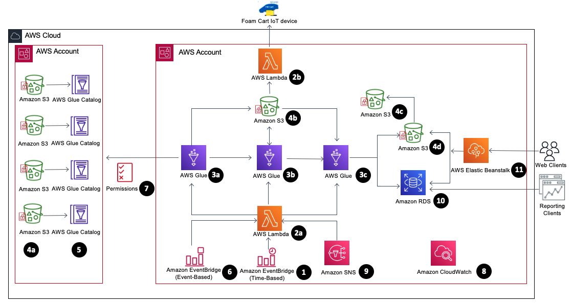
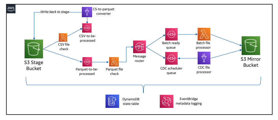
The following diagram illustrates the architecture of our wash analytics solution using AWS services.

The solution includes the following components:

  • EventBridge (1) – We use an EventBridge (time-based) to schedule the daily process to capture the delta changes between the runs.
  • Lambda (2a) – Lambda orchestrates the AWS Glue jobs initiation, backup, and recovery on failure for each stage, utilizing EventBridge (event-based) for the alerting of these events.
  • Lambda (2b) – Foam cart events from IoT devices are loaded into staging buckets in Amazon Simple Storage Service (Amazon S3) daily.
  • AWS Glue (3) – The wash analytics need to handle a small subset of data daily, but the initial historical load and transformation is huge. Because AWS Glue is serverless, it’s easy to set up and run with no maintenance.
    • Copy job (3a) – We use an AWS Glue copy job to copy only the required subset of data from across AWS accounts by connecting to AWS Glue Data Catalog tables using a cross-account AWS Identity and Access Management (IAM) role.
    • Business transformation jobs (3b, 3c) – When the copy job is complete, Lambda triggers subsequent AWS Glue jobs. Because our jobs are both compute and memory intensive, we use G2.x worker nodes. We can use Amazon CloudWatch metrics to fine-tune our jobs to use the right worker nodes. To handle complex calculations, we split large jobs up into multiple jobs by pipelining the output of one job as input to another job.
  • Source S3 buckets (4a) – Flights, wash events, and other engine parameter data is available in source buckets in a different AWS account exposed via Data Catalog tables.
  • Stage S3 bucket (4b) – Data from another AWS account is required for calculations, and all the intermediate outputs from the AWS Glue jobs are written to the staging bucket.
  • Backup S3 bucket (4c) – Every day before starting the AWS Glue job, the previous day’s output from the output bucket is backed up in the backup bucket. In case of any job failure, the data is recovered from this bucket.
  • Output S3 bucket (4d) – The final output from the AWS Glue jobs is written to the output bucket.

Continuing our analysis of the architecture components, we also use the following:

  • AWS Glue Data Catalog tables (5) – We catalog flights, wash events, and other engine parameter data using Data Catalog tables, which are accessed by AWS Glue copy jobs from another AWS account.
  • EventBridge (6) – We use EventBridge (event-based) to monitor for AWS Glue job state changes (SUCEEDED, FAILED, TIMEOUT, and STOPPED) and orchestrate the workflow, including backup, recovery, and job status notifications.
  • IAM role (7) – We set up cross-account IAM roles to copy the data from one account to another from the AWS Glue Data Catalog tables.
  • CloudWatch metrics (8) – You can monitor many different CloudWatch metrics. The following metrics can help you decide on horizontal or vertical scaling when fine-tuning the AWS Glue jobs:
    • CPU load of the driver and executors
    • Memory profile of the driver
    • ETL data movement
    • Data shuffle across executors
    • Job run metrics, including active executors, completed stages, and maximum needed executors
  • Amazon SNS (9) Amazon Simple Notification Service (Amazon SNS) automatically sends notifications to the support group on the error status of jobs, so they can take corrective action upon failure.
  • Amazon RDS (10) – The final transformed data is stored in Amazon Relational Database Service (Amazon RDS) for PostgreSQL (in addition to Amazon S3) to support legacy reporting tools.
  • Web application (11) – A web application is hosted on AWS Elastic Beanstalk, and is enabled with Auto Scaling exposed for clients to access the analytics data.

Implementation strategy

Implementing our solution included the following considerations:

  • Security – The data required for running analytics is present in different data sources and different AWS accounts. We needed to craft well-thought-out role-based access policies for accessing the data.
  • Selecting the right programming paradigm – PySpark does lazy evaluation while working with data frames. For PySpark to work efficiently with AWS Glue, we created data frames with required columns upfront and performed column-wise operations.
  • Choosing the right persistence storage – Writing to Amazon S3 enables multiple consumption patterns, and writes are much faster due to parallelism.

If we’re writing to Amazon RDS (for supporting legacy systems), we need to watch out for database connectivity and buffer lock issues while writing from AWS Glue jobs.

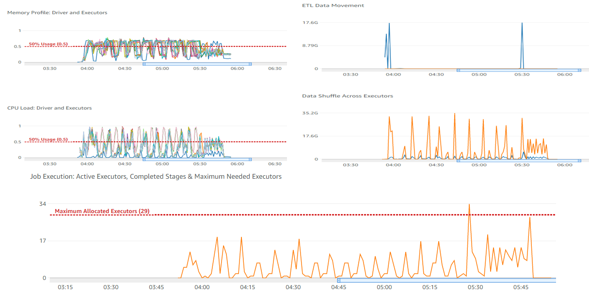
  • Data partitioning – Identifying the right key combination is important for partitioning the data for Spark to perform optimally. Our initial runs (without data partition) with 30 workers of type G2.x took 2 hours and 4 minutes to complete.

The following screenshot shows our CloudWatch metrics.

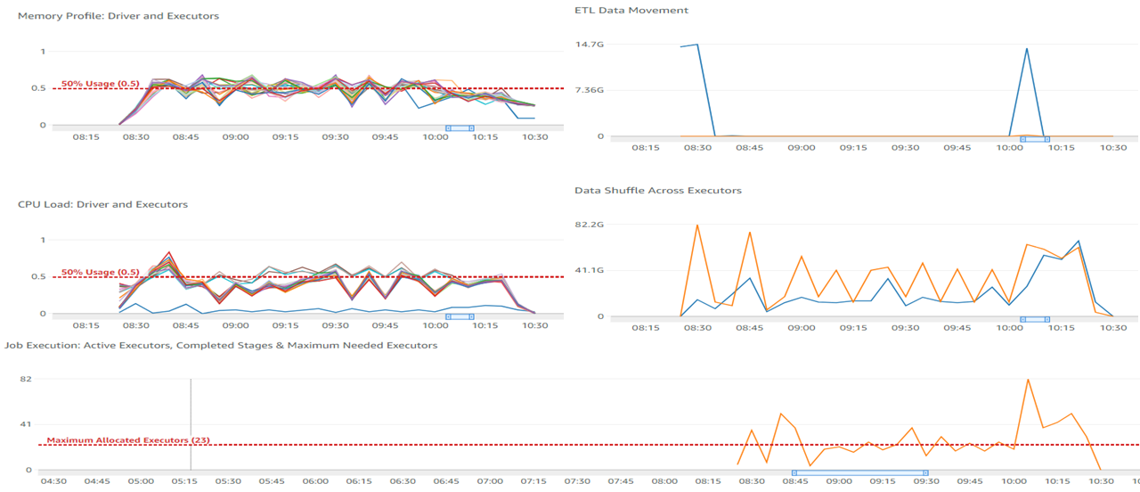
After a few dry runs, we were able to arrive at partitioning by a specific column (df.repartition(columnKey)) and with 24 workers of type G2.x, the job completed in 2 hours and 7 minutes. The following screenshot shows our new metrics.

We can observe a difference in CPU and memory utilization—running with even fewer nodes shows a smaller CPU utilization and memory footprint.

The following table shows how we achieved the final transformation with the strategies we discussed.

Iteration Run Time AWS Glue Job Status Strategy
1 ~12 hours Unsuccessful/Stopped Initial iteration
2 ~9 hours Unsuccessful/Stopped Changing code to PySpark methodology
3 5 hours, 11 minutes Partial success Splitting a complex large job into multiple jobs
4 3 hours, 33 minutes Success Partitioning by column key
5 2 hours, 39 minutes Success Changing CSV to Parquet file format while storing the copied data from another AWS account and intermediate results in the stage S3 bucket
6 2 hours, 9 minutes Success Infra scaling: horizontal and vertical scaling

Conclusion

In this post, we saw how to build a cost-effective, maintenance-free solution using serverless AWS services to process large-scale data. We also learned how to gain optimal AWS Glue job performance with key partitioning, using the Parquet data format while persisting in Amazon S3, splitting complex jobs into multiple jobs, and using the right programming paradigm.

As we continue to solidify our data lake solution for data from various sources, we can use Amazon Redshift Spectrum to serve various future analytical use cases.


About the Authors

Giridhar G Jorapur is a Staff Infrastructure Architect at GE Aviation. In this role, he is responsible for designing enterprise applications, migration and modernization of applications to the cloud. Apart from work, Giri enjoys investing himself in spiritual wellness. Connect him on LinkedIn.

How ENGIE scales their data ingestion pipelines using Amazon MWAA

Post Syndicated from Anouar Zaaber original https://aws.amazon.com/blogs/big-data/how-engie-scales-their-data-ingestion-pipelines-using-amazon-mwaa/

ENGIE—one of the largest utility providers in France and a global player in the zero-carbon energy transition—produces, transports, and deals electricity, gas, and energy services. With 160,000 employees worldwide, ENGIE is a decentralized organization and operates 25 business units with a high level of delegation and empowerment. ENGIE’s decentralized global customer base had accumulated lots of data, and it required a smarter, unique approach and solution to align its initiatives and provide data that is ingestible, organizable, governable, sharable, and actionable across its global business units.

In 2018, the company’s business leadership decided to accelerate its digital transformation through data and innovation by becoming a data-driven company. Yves Le Gélard, chief digital officer at ENGIE, explains the company’s purpose: “Sustainability for ENGIE is the alpha and the omega of everything. This is our raison d’être. We help large corporations and the biggest cities on earth in their attempts to transition to zero carbon as quickly as possible because it is actually the number one question for humanity today.”

ENGIE, as with any other big enterprise, is using multiple extract, transform, and load (ETL) tools to ingest data into their data lake on AWS. Nevertheless, they usually have expensive licensing plans. “The company needed a uniform method of collecting and analyzing data to help customers manage their value chains,” says Gregory Wolowiec, the Chief Technology Officer who leads ENGIE’s data program. ENGIE wanted a free-license application, well integrated with multiple technologies and with a continuous integration, continuous delivery (CI/CD) pipeline to more easily scale all their ingestion process.

ENGIE started using Amazon Managed Workflows for Apache Airflow (Amazon MWAA) to solve this issue and started moving various data sources from on-premise applications and ERPs, AWS services like Amazon Redshift, Amazon Relational Database Service (Amazon RDS), Amazon DynamoDB, external services like Salesforce, and other cloud providers to a centralized data lake on top of Amazon Simple Storage Service (Amazon S3).

Amazon MWAA is used in particular to collect and store harmonized operational and corporate data from different on-premises and software as a service (SaaS) data sources into a centralized data lake. The purpose of this data lake is to create a “group performance cockpit” that enables an efficient, data-driven analysis and thoughtful decision-making by the Engie Management board.

In this post, we share how ENGIE created a CI/CD pipeline for an Amazon MWAA project template using an AWS CodeCommit repository and plugged it into AWS CodePipeline to build, test, and package the code and custom plugins. In this use case, we developed a custom plugin to ingest data from Salesforce based on the Airflow Salesforce open-source plugin.

Solution overview

The following diagrams illustrate the solution architecture defining the implemented Amazon MWAA environment and its associated pipelines. It also describes the customer use case for Salesforce data ingestion into Amazon S3.

The following diagram shows the architecture of the deployed Amazon MWAA environment and the implemented pipelines.

The preceding architecture is fully deployed via infrastructure as code (IaC). The implementation includes the following:

  • Amazon MWAA environment – A customizable Amazon MWAA environment packaged with plugins and requirements and configured in a secure manner.
  • Provisioning pipeline – The admin team can manage the Amazon MWAA environment using the included CI/CD provisioning pipeline. This pipeline includes a CodeCommit repository plugged into CodePipeline to continuously update the environment and its plugins and requirements.
  • Project pipeline – This CI/CD pipeline comes with a CodeCommit repository that triggers CodePipeline to continuously build, test and deploy DAGs developed by users. Once deployed, these DAGs are made available in the Amazon MWAA environment.

The following diagram shows the data ingestion workflow, which includes the following steps:

  1. The DAG is triggered by Amazon MWAA manually or based on a schedule.
  2. Amazon MWAA initiates data collection parameters and calculates batches.
  3. Amazon MWAA distributes processing tasks among its workers.
  4. Data is retrieved from Salesforce in batches.
  5. Amazon MWAA assumes an AWS Identity and Access Management (IAM) role with the necessary permissions to store the collected data into the target S3 bucket.

This AWS Cloud Development Kit (AWS CDK) construct is implemented with the following security best practices:

  • With the principle of least privilege, you grant permissions to only the resources or actions that users need to perform tasks.
  • S3 buckets are deployed with security compliance rules: encryption, versioning, and blocking public access.
  • Authentication and authorization management is handled with AWS Single Sign-On (AWS SSO).
  • Airflow stores connections to external sources in a secure manner either in Airflow’s default secrets backend or an alternative secrets backend such as AWS Secrets Manager or AWS Systems Manager Parameter Store.

For this post, we step through a use case using the data from Salesforce to ingest it into an ENGIE data lake in order to transform it and build business reports.

Prerequisites for deployment

For this walkthrough, the following are prerequisites:

  • Basic knowledge of the Linux operating system
  • Access to an AWS account with administrator or power user (or equivalent) IAM role policies attached
  • Access to a shell environment or optionally with AWS CloudShell

Deploy the solution

To deploy and run the solution, complete the following steps:

  1. Install AWS CDK.
  2. Bootstrap your AWS account.
  3. Define your AWS CDK environment variables.
  4. Deploy the stack.

Install AWS CDK

The described solution is fully deployed with AWS CDK.

AWS CDK is an open-source software development framework to model and provision your cloud application resources using familiar programming languages. If you want to familiarize yourself with AWS CDK, the AWS CDK Workshop is a great place to start.

Install AWS CDK using the following commands:

npm install -g aws-cdk
# To check the installation
cdk --version

Bootstrap your AWS account

First, you need to make sure the environment where you’re planning to deploy the solution to has been bootstrapped. You only need to do this one time per environment where you want to deploy AWS CDK applications. If you’re unsure whether your environment has been bootstrapped already, you can always run the command again:

cdk bootstrap aws://YOUR_ACCOUNT_ID/YOUR_REGION

Define your AWS CDK environment variables

On Linux or MacOS, define your environment variables with the following code:

export CDK_DEFAULT_ACCOUNT=YOUR_ACCOUNT_ID
export CDK_DEFAULT_REGION=YOUR_REGION

On Windows, use the following code:

setx CDK_DEFAULT_ACCOUNT YOUR_ACCOUNT_ID
setx CDK_DEFAULT_REGION YOUR_REGION

Deploy the stack

By default, the stack deploys a basic Amazon MWAA environment with the associated pipelines described previously. It creates a new VPC in order to host the Amazon MWAA resources.

The stack can be customized using the parameters listed in the following table.

To pass a parameter to the construct, you can use the AWS CDK runtime context. If you intend to customize your environment with multiple parameters, we recommend using the cdk.json context file with version control to avoid unexpected changes to your deployments. Throughout our example, we pass only one parameter to the construct. Therefore, for the simplicity of the tutorial, we use the the --context or -c option to the cdk command, as in the following example:

cdk deploy -c paramName=paramValue -c paramName=paramValue ...
Parameter Description Default Valid values
vpcId VPC ID where the cluster is deployed. If none, creates a new one and needs the parameter cidr in that case. None VPC ID
cidr The CIDR for the VPC that is created to host Amazon MWAA resources. Used only if the vpcId is not defined. 172.31.0.0/16 IP CIDR
subnetIds Comma-separated list of subnets IDs where the cluster is deployed. If none, looks for private subnets in the same Availability Zone. None Subnet IDs list (coma separated)
envName Amazon MWAA environment name MwaaEnvironment String
envTags Amazon MWAA environment tags None See the following JSON example: '{"Environment":"MyEnv", "Application":"MyApp", "Reason":"Airflow"}'
environmentClass Amazon MWAA environment class mw1.small mw1.small, mw1.medium, mw1.large
maxWorkers Amazon MWAA maximum workers 1 int
webserverAccessMode Amazon MWAA environment access mode (private or public) PUBLIC_ONLY PUBLIC_ONLY, PRIVATE_ONLY
secretsBackend Amazon MWAA environment secrets backend Airflow SecretsManager

Clone the GitHub repository:

git clone https://github.com/aws-samples/cdk-amazon-mwaa-cicd

Deploy the stack using the following command:

cd mwaairflow && \
pip install . && \
cdk synth && \
cdk deploy -c vpcId=YOUR_VPC_ID

The following screenshot shows the stack deployment:

The following screenshot shows the deployed stack:

Create solution resources

For this walkthrough, you should have the following prerequisites:

If you don’t have a Salesforce account, you can create a SalesForce developer account:

  1. Sign up for a developer account.
  2. Copy the host from the email that you receive.
  3. Log in into your new Salesforce account
  4. Choose the profile icon, then Settings.
  5. Choose Reset my Security Token.
  6. Check your email and copy the security token that you receive.

After you complete these prerequisites, you’re ready to create the following resources:

  • An S3 bucket for Salesforce output data
  • An IAM role and IAM policy to write the Salesforce output data on Amazon S3
  • A Salesforce connection on the Airflow UI to be able to read from Salesforce
  • An AWS connection on the Airflow UI to be able to write on Amazon S3
  • An Airflow variable on the Airflow UI to store the name of the target S3 bucket

Create an S3 bucket for Salesforce output data

To create an output S3 bucket, complete the following steps:

  1. On the Amazon S3 console, choose Create bucket.

The Create bucket wizard opens.

  1. For Bucket name, enter a DNS-compliant name for your bucket, such as airflow-blog-post.
  2. For Region, choose the Region where you deployed your Amazon MWAA environment, for example, US East (N. Virginia) us-east-1.
  3. Choose Create bucket.

For more information, see Creating a bucket.

Create an IAM role and IAM policy to write the Salesforce output data on Amazon S3

In this step, we create an IAM policy that allows Amazon MWAA to write on your S3 bucket.

  1. On the IAM console, in the navigation pane, choose Policies.
  2. Choose Create policy.
  3. Choose the JSON tab.
  4. Enter the following JSON policy document, and replace airflow-blog-post with your bucket name:
    {
      "Version": "2012-10-17",
      "Statement": [
        {
          "Effect": "Allow",
          "Action": ["s3:ListBucket"],
          "Resource": ["arn:aws:s3:::airflow-blog-post"]
        },
        {
          "Effect": "Allow",
          "Action": [
            "s3:PutObject",
            "s3:GetObject",
            "s3:DeleteObject"
          ],
          "Resource": ["arn:aws:s3:::airflow-blog-post/*"]
        }
      ]
    }

  5. Choose Next: Tags.
  6. Choose Next: Review.
  7. For Name, choose a name for your policy (for example, airflow_data_output_policy).
  8. Choose Create policy.

Let’s attach the IAM policy to a new IAM role that we use in our Airflow connections.

  1. On the IAM console, choose Roles in the navigation pane and then choose Create role.
  2. In the Or select a service to view its use cases section, choose S3.
  3. For Select your use case, choose S3.
  4. Search for the name of the IAM policy that we created in the previous step (airflow_data_output_role) and select the policy.
  5. Choose Next: Tags.
  6. Choose Next: Review.
  7. For Role name, choose a name for your role (airflow_data_output_role).
  8. Review the role and then choose Create role.

You’re redirected to the Roles section.

  1. In the search box, enter the name of the role that you created and choose it.
  2. Copy the role ARN to use later to create the AWS connection on Airflow.

Create a Salesforce connection on the Airflow UI to be able to read from Salesforce

To read data from Salesforce, we need to create a connection using the Airflow user interface.

  1. On the Airflow UI, choose Admin.
  2. Choose Connections, and then the plus sign to create a new connection.
  3. Fill in the fields with the required information.

The following table provides more information about each value.

Field Mandatory Description Values
Conn Id Yes Connection ID to define and to be used later in the DAG For example, salesforce_connection
Conn Type Yes Connection type HTTP
Host Yes Salesforce host name host-dev-ed.my.salesforce.com or host.lightning.force.com. Replace the host with your Salesforce host and don’t add the http:// as prefix.
Login Yes The Salesforce user name. The user must have read access to the salesforce objects. [email protected]
Password Yes The corresponding password for the defined user. MyPassword123
Port No Salesforce instance port. By default, 443. 443
Extra Yes Specify the extra parameters (as a JSON dictionary) that can be used in the Salesforce connection. security_token is the Salesforce security token for authentication. To get the Salesforce security token in your email, you must reset your security token. {"security_token":"AbCdE..."}

Create an AWS connection in the Airflow UI to be able to write on Amazon S3

An AWS connection is required to upload data into Amazon S3, so we need to create a connection using the Airflow user interface.

  1. On the Airflow UI, choose Admin.
  2. Choose Connections, and then choose the plus sign to create a new connection.
  3. Fill in the fields with the required information.

The following table provides more information about the fields.

Field Mandatory Description Value
Conn Id Yes Connection ID to define and to be used later in the DAG For example, aws_connection
Conn Type Yes Connection type Amazon Web Services
Extra Yes It is required to specify the Region. You also need to provide the role ARN that we created earlier.
{
"region":"eu-west-1",
"role_arn":"arn:aws:iam::123456789101:role/airflow_data_output_role "
}

Create an Airflow variable on the Airflow UI to store the name of the target S3 bucket

We create a variable to set the name of the target S3 bucket. This variable is used by the DAG. So, we need to create a variable using the Airflow user interface.

  1. On the Airflow UI, choose Admin.
  2. Choose Variables, then choose the plus sign to create a new variable.
  3. For Key, enter bucket_name.
  4. For Val, enter the name of the S3 bucket that you created in a previous step (airflow-blog-post).

Create and deploy a DAG in Amazon MWAA

To be able to ingest data from Salesforce into Amazon S3, we need to create a DAG (Directed Acyclic Graph). To create and deploy the DAG, complete the following steps:

  1. Create a local Python DAG.
  2. Deploy your DAG using the project CI/CD pipeline.
  3. Run your DAG on the Airflow UI.
  4. Display your data in Amazon S3 (with S3 Select).

Create a local Python DAG

The provided SalesForceToS3Operator allows you to ingest data from Salesforce objects to an S3 bucket. Refer to standard Salesforce objects for the full list of objects you can ingest data from with this Airflow operator.

In this use case, we ingest data from the Opportunity Salesforce object. We retrieve the last 6 months’ data in monthly batches and we filter on a specific list of fields.

The DAG provided in the sample in GitHub repository imports the last 6 months of the Opportunity object (one file by month) by filtering the list of retrieved fields.

This operator takes two connections as parameters:

  • An AWS connection that is used to upload ingested data into Amazon S3.
  • A Salesforce connection to read data from Salesforce.

The following table provides more information about the parameters.

Parameter Type Mandatory Description
sf_conn_id string Yes Name of the Airflow connection that has the following information:

  • user name
  • password
  • security token
sf_obj string Yes Name of the relevant Salesforce object (Account, Lead, Opportunity)
s3_conn_id string Yes The destination S3 connection ID
s3_bucket string Yes The destination S3 bucket
s3_key string Yes The destination S3 key
sf_fields string No The (optional) list of fields that you want to get from the object (Id, Name, and so on).
If none (the default), then this gets all fields for the object.
fmt string No The (optional) format that the S3 key of the data should be in.
Possible values include CSV (default), JSON, and NDJSON.
from_date date format No A specific date-time (optional) formatted input to run queries from for incremental ingestion.
Evaluated against the SystemModStamp attribute.
Not compatible with the query parameter and should be in date-time format (for example, 2021-01-01T00:00:00Z).
Default: None
to_date date format No A specific date-time (optional) formatted input to run queries to for incremental ingestion.
Evaluated against the SystemModStamp attribute.
Not compatible with the query parameter and should be in date-time format (for example, 2021-01-01T00:00:00Z).
Default: None
query string No A specific query (optional) to run for the given object.
This overrides default query creation.
Default: None
relationship_object string No Some queries require relationship objects to work, and these are not the same names as the Salesforce object.
Specify that relationship object here (optional).
Default: None
record_time_added boolean No Set this optional value to true if you want to add a Unix timestamp field to the resulting data that marks when the data was fetched from Salesforce.
Default: False
coerce_to_timestamp boolean No Set this optional value to true if you want to convert all fields with dates and datetimes into Unix timestamp (UTC).
Default: False

The first step is to import the operator in your DAG:

from operators.salesforce_to_s3_operator import SalesforceToS3Operator

Then define your DAG default ARGs, which you can use for your common task parameters:

# These args will get passed on to each operator
# You can override them on a per-task basis during operator initialization
default_args = {
    'owner': '[email protected]',
    'depends_on_past': False,
    'start_date': days_ago(2),
    'retries': 0,
    'retry_delay': timedelta(minutes=1),
    'sf_conn_id': 'salesforce_connection',
    's3_conn_id': 'aws_connection',
    's3_bucket': 'salesforce-to-s3',
}
...

Finally, you define the tasks to use the operator.

The following examples illustrate some use cases.

Salesforce object full ingestion

This task ingests all the content of the Salesforce object defined in sf_obj. This selects all the object’s available fields and writes them into the defined format in fmt. See the following code:

...
salesforce_to_s3 = SalesforceToS3Operator(
    task_id="Opportunity_to_S3",
    sf_conn_id=default_args["sf_conn_id"],
    sf_obj="Opportunity",
    fmt="ndjson",
    s3_conn_id=default_args["s3_conn_id"],
    s3_bucket=default_args["s3_bucket"],
    s3_key=f"salesforce/raw/dt={s3_prefix}/{table.lower()}.json",
    dag=salesforce_to_s3_dag,
)
...

Salesforce object partial ingestion based on fields

This task ingests specific fields of the Salesforce object defined in sf_obj. The selected fields are defined in the optional sf_fields parameter. See the following code:

...
salesforce_to_s3 = SalesforceToS3Operator(
    task_id="Opportunity_to_S3",
    sf_conn_id=default_args["sf_conn_id"],
    sf_obj="Opportunity",
    sf_fields=["Id","Name","Amount"],
    fmt="ndjson",
    s3_conn_id=default_args["s3_conn_id"],
    s3_bucket=default_args["s3_bucket"],
    s3_key=f"salesforce/raw/dt={s3_prefix}/{table.lower()}.json",
    dag=salesforce_to_s3_dag,
)
...

Salesforce object partial ingestion based on time period

This task ingests all the fields of the Salesforce object defined in sf_obj. The time period can be relative using from_date or to_date parameters or absolute by using both parameters.

The following example illustrates relative ingestion from the defined date:

...
salesforce_to_s3 = SalesforceToS3Operator(
    task_id="Opportunity_to_S3",
    sf_conn_id=default_args["sf_conn_id"],
    sf_obj="Opportunity",
    from_date="YESTERDAY",
    fmt="ndjson",
    s3_conn_id=default_args["s3_conn_id"],
    s3_bucket=default_args["s3_bucket"],
    s3_key=f"salesforce/raw/dt={s3_prefix}/{table.lower()}.json",
    dag=salesforce_to_s3_dag,
)
...

The from_date and to_date parameters support Salesforce date-time format. It can be either a specific date or literal (for example TODAY, LAST_WEEK, LAST_N_DAYS:5). For more information about date formats, see Date Formats and Date Literals.

For the full DAG, refer to the sample in GitHub repository.

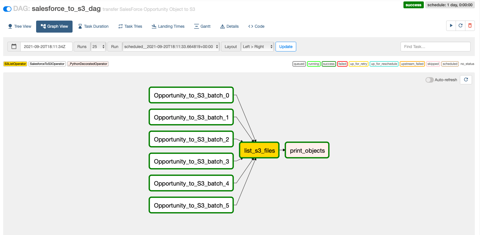
This code dynamically generates tasks that run queries to retrieve the data of the Opportunity object in the form of 1-month batches.

The sf_fields parameter allows us to extract only the selected fields from the object.

Save the DAG locally as salesforce_to_s3.py.

Deploy your DAG using the project CI/CD pipeline

As part of the CDK deployment, a CodeCommit repository and CodePipeline pipeline were created in order to continuously build, test, and deploy DAGs into your Amazon MWAA environment.

To deploy the new DAG, the source code should be committed to the CodeCommit repository. This triggers a CodePipeline run that builds, tests, and deploys your new DAG and makes it available in your Amazon MWAA environment.

  1. Sign in to the CodeCommit console in your deployment Region.
  2. Under Source, choose Repositories.

You should see a new repository mwaaproject.

  1. Push your new DAG in the mwaaproject repository under dags. You can either use the CodeCommit console or the Git command line to do so:
    1. CodeCommit console:
      1. Choose the project CodeCommit repository name mwaaproject and navigate under dags.
      2. Choose Add file and then Upload file and upload your new DAG.
    2. Git command line:
      1. To be able to clone and access your CodeCommit project with the Git command line, make sure Git client is properly configured. Refer to Setting up for AWS CodeCommit.
      2. Clone the repository with the following command after replacing <region> with your project Region:
        git clone https://git-codecommit.<region>.amazonaws.com/v1/repos/mwaaproject

      3. Copy the DAG file under dags and add it with the command:
        git add dags/salesforce_to_s3.py

      4. Commit your new file with a message:
        git commit -m "add salesforce DAG"

      5. Push the local file to the CodeCommit repository:
        git push

The new commit triggers a new pipeline that builds, tests, and deploys the new DAG. You can monitor the pipeline on the CodePipeline console.

  1. On the CodePipeline console, choose Pipeline in the navigation pane.
  2. On the Pipelines page, you should see mwaaproject-pipeline.
  3. Choose the pipeline to display its details.

After checking that the pipeline run is successful, you can verify that the DAG is deployed to the S3 bucket and therefore available on the Amazon MWAA console.

  1. On the Amazon S3 console, look for a bucket starting with mwaairflowstack-mwaaenvstackne and go under dags.

You should see the new DAG.

  1. On the Amazon MWAA console, choose DAGs.

You should be able to see the new DAG.

Run your DAG on the Airflow UI

Go to the Airflow UI and toggle on the DAG.

This triggers your DAG automatically.

Later, you can continue manually triggering it by choosing the run icon.

Choose the DAG and Graph View to see the run of your DAG.

If you have any issue, you can check the logs of the failed tasks from the task instance context menu.

Display your data in Amazon S3 (with S3 Select)

To display your data, complete the following steps:

  1. On the Amazon S3 console, in the Buckets list, choose the name of the bucket that contains the output of the Salesforce data (airflow-blog-post).
  2. In the Objects list, choose the name of the folder that has the object that you copied from Salesforce (opportunity).
  3. Choose the raw folder and the dt folder with the latest timestamp.
  4. Select any file.
  5. On the Actions menu, choose Query with S3 Select.
  6. Choose Run SQL query to preview the data.

Clean up

To avoid incurring future charges, delete the AWS CloudFormation stack and the resources that you deployed as part of this post.

  1. On the AWS CloudFormation console, delete the stack MWAAirflowStack.

To clean up the deployed resources using the AWS Command Line Interface (AWS CLI), you can simply run the following command:

cdk destroy MWAAirflowStack

Make sure you are in the root path of the project when you run the command.

After confirming that you want to destroy the CloudFormation stack, the solution’s resources are deleted from your AWS account.

The following screenshot shows the process of deploying the stack:

The following screenshot confirms the stack is undeployed.

  1. Navigate to the Amazon S3 console and locate the two buckets containing mwaairflowstack-mwaaenvstack and mwaairflowstack-mwaaproj that were created during the deployment.
  2. Select each bucket delete its contents, then delete the bucket.
  3. Delete the IAM role created to write on the S3 buckets.

Conclusion

ENGIE discovered significant value by using Amazon MWAA, enabling its global business units to ingest data in more productive ways. This post presented how ENGIE scaled their data ingestion pipelines using Amazon MWAA. The first part of the post described the architecture components and how to successfully deploy a CI/CD pipeline for an Amazon MWAA project template using a CodeCommit repository and plug it into CodePipeline to build, test, and package the code and custom plugins. The second part walked you through the steps to automate the ingestion process from Salesforce using Airflow with an example. For the Airflow configuration, you used Airflow variables, but you can also use Secrets Manager with Amazon MWAA using the secretsBackend parameter when deploying the stack.

The use case discussed in this post is just one example of how you can use Amazon MWAA to make it easier to set up and operate end-to-end data pipelines in the cloud at scale. For more information about Amazon MWAA, check out the User Guide.


About the Authors

Anouar Zaaber is a Senior Engagement Manager in AWS Professional Services. He leads internal AWS, external partner, and customer teams to deliver AWS cloud services that enable the customers to realize their business outcomes.

Amine El Mallem is a Data/ML Ops Engineer in AWS Professional Services. He works with customers to design, automate, and build solutions on AWS for their business needs.

Armando Segnini is a Data Architect with AWS Professional Services. He spends his time building scalable big data and analytics solutions for AWS Enterprise and Strategic customers. Armando also loves to travel with his family all around the world and take pictures of the places he visits.

Mohamed-Ali Elouaer is a DevOps Consultant with AWS Professional Services. He is part of the AWS ProServe team, helping enterprise customers solve complex problems related to automation, security, and monitoring using AWS services. In his free time, he likes to travel and watch movies.

Julien Grinsztajn is an Architect at ENGIE. He is part of the Digital & IT Consulting ENGIE IT team working on the definition of the architecture for complex projects related to data integration and network security. In his free time, he likes to travel the oceans to meet sharks and other marine creatures.

Monitoring Juniper Mist wireless network

Post Syndicated from Brian van Baekel original https://blog.zabbix.com/monitoring-juniper-mist-wireless-network/19093/

As Premium Zabbix partner, Opensource ICT Solutions is building Zabbix solutions all over the world. That means we have customers with a broad variety of requirements, thoughts on how to monitor things, which metrics are important and how to alert upon it. If one of those customers approaches us with a question concerning a task the likes of which we have never done before, it’s a challenge. And we love challenges! This blog post will cover one such challenge that we solved some time ago.

Quanza is a leading infrastructure operator offering a broad portfolio of services to completely take over the management of networks, data centers and cloud services. With more than 70 colleagues and at least as many specializations, everyone at Quanza works towards the same goal: designing, building, and operating an optimal IT infrastructure. Exactly like you would expect it… and then some. Quanza understands that you prefer to focus on your own innovation. By continuously mapping out your wishes, Quanza provides customized solutions that keep your network up and running 24×7. Today and in the future.

With a relentless focus on mission-critical environments, often of relevance to society, Quanza has an impressive line-up of customers. Some enterprises that chose to partner up with Quanza are SURF, Payvision, the Volksbank, and the Amsterdam Internet Exchange (AMS-IX), one of the world’s largest internet hubs.

Recently, customers started asking Quanza to embed Juniper MIST products for wired and wireless networks in their service portfolio. In order to fully support the network’s lifecycle (build, operate and innovate), the Juniper MIST products will need to be monitored by their 24×7 NOC. This is where we came into play, with our Zabbix knowledge.

We quickly decided to combine the knowledge Quanza has of the Juniper MIST equipment and API and our Zabbix knowledge to build the best possible monitoring solution.

SNMP or cloud?

The Juniper MIST solution is a cloud-based solution that provides a single pane of management for Juniper Networks products. As it’s cloud-based, it’s not a “traditional” network solution. As such, SNMP is not an option for device monitoring as they are communicating only with “the cloud” and we cannot access them directly like we used to do with traditional network equipment.

So, we started to investigate other options. One of the most common options right now is talking to some sort of API and pulling the metrics from that API. With Zabbix “HTTP agent” item key, this is no problem at all. Unfortunately, that’s not how the MIST API works. It’s pushing data instead of letting you pull it (actually, it does – but this doesn’t scale at all). Now, the Zabbix HTTP Agent item type allows trapping, but only in a specific Zabbix sender format. Of course, the MIST API does not allow that.

This means we have a problem. SNMP is not available. Pulling data is not a viable, scalable option. Pushing the data is an option, but Zabbix does not understand that.

Since we are not talking about some sort of proprietary monitoring tool which is completely closed and way too static, there is always a solution with Zabbix as long as you’re creative enough.

Getting data into Zabbix

We needed some middleware. Something that was able to receive that data from MIST and convert it into something that we can push into Zabbix.

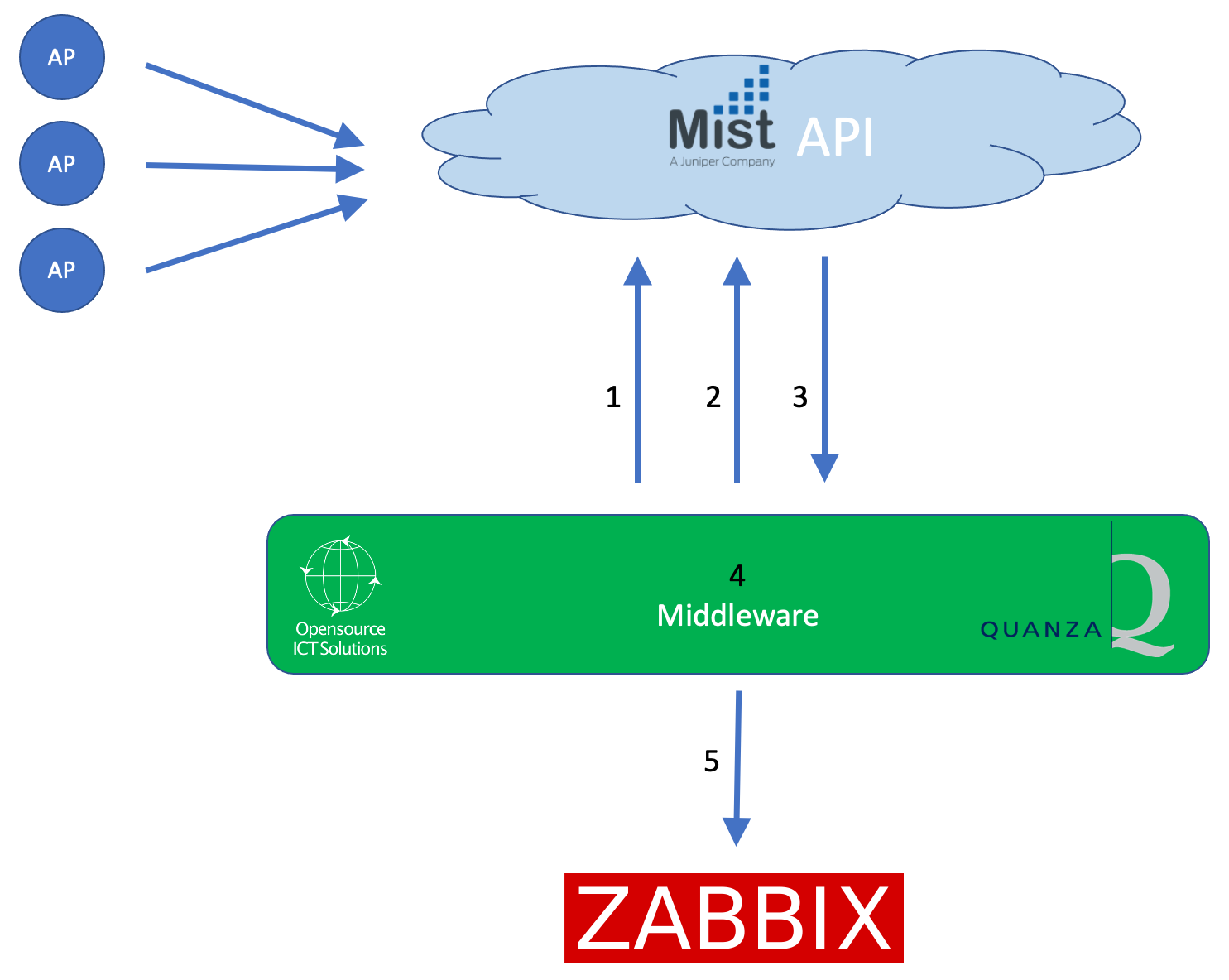
That’s exactly what we did. We, together with Quanza, built a middleware that uses an API token to authenticate against the MIST API endpoint. Once the authentication is successful, the middleware is allowed to subscribe to certain “channels”. These channels provide event and performance data. You can compare it with MQTT, where a subscription to channels/topics is needed to get the information you are interested in.

Mist Middleware explained

  • Step 1:  Authenticate using an API token.
  • Step 2: Subscribe to channels
  • Step 3: Receive performance and event data
  • Step 4: Filter out only the relevant (performance) data for Zabbix
  • Step 5: Push into Zabbix

Once we had this in place, the MIST part was finished. We had our data and were able to push it into the monitoring solution.

Parsing in Zabbix

So, right now we have the data available for Zabbix. Time to find a neat way to use it. As the environments (both inventory and the types of equipment that are used) might be dynamic, we definitely do not want to apply any manual work to monitor newly added sites/equipment.

That means that low-level discovery rules are pretty much the only viable solution.

Here we go:

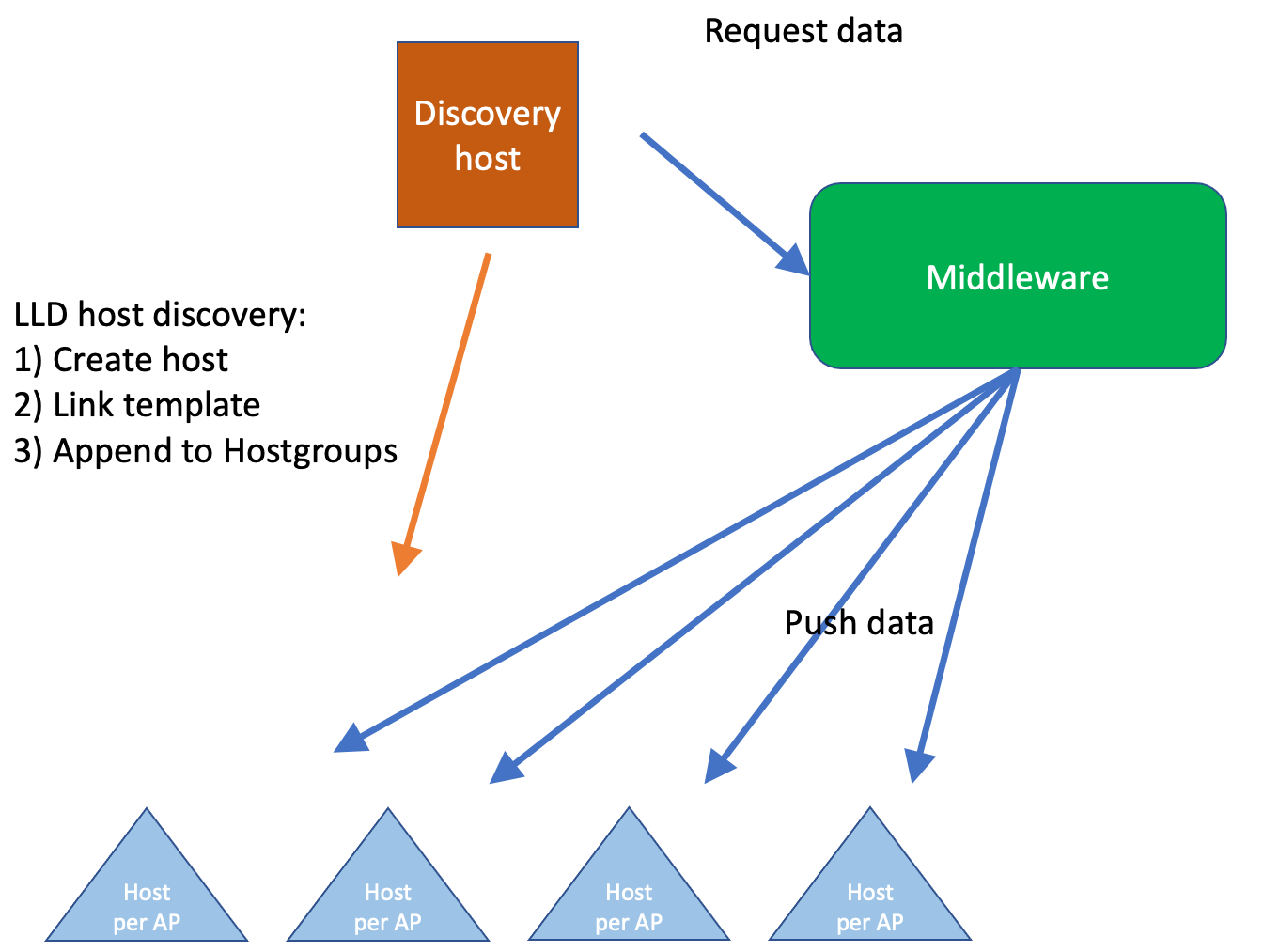
Describing host prototypes


Within Zabbix, we configure 1 host (the Discovery host) and apply a template on that host, with exactly 1 LLD rule: Query our middleware, and based on the information received, create new hosts (Host prototypes).

The data that is received looks like this:

{
"NODEID":"<NODEID>",
"NAME":"AP-<SITE>-<NUMBER",
"SITENAME":"<SITENAME>",
"SITEID":"<SITEID>",
"MAC":"<MAC ADDRESS>",
"ORGNAME":"<ORG NAME>"
},

Those new/discovered hosts will have the names of the AP and corresponding organization and location (in Mist: site). We also link a template to the discovered host and add it to a Host group with the variables we’ll need later, such as the organization, site name, siteID etc.

So, We need to parse those JSON elements. Luckily Zabbix provides, within the LLD rule config the option to parse this into LLD macros, so for example the Node id is parsed into {#ID} with the use of JSONPath $.NODEID:

LLD macro configuration

Once this process is complete, we have a new host per AP. Of course, there is no data on that host and querying the middleware or Mist is a bad idea. Scalability will be extremely problematic with more than a few organizations and sites configured in the Mist environment. As we’re building this with a big network integrator, scalability is a thing and we do not want to risk having a noticeable performance impact by using polling.

How about pushing data from the middleware into Zabbix? Once the data is received from Mist by the middleware, it’s parsed, filtered and then it pushes out whatever must be pushed out to Zabbix. We decided the best option is to push per host as we have those already available in Zabbix.

Now we should ensure two things:

    • do not overwhelm Zabbix with data being pushed in
    • Getting all the data with the least number of ‘pushes’ into Zabbix

Again, the flexibility of Zabbix is extremely useful here. On the AP hosts, there is a template with exactly 1 trapper item: receive performance data. From there, everything will be handled by the Zabbix ‘Master/Dependent’ item concept. We then extract data like temperatures, CPU load, memory usage, etc.

At the same time, we receive data regarding network usage (interface statistics) and radio information. As we do not know upfront how many network interfaces and radio’s there are on a particular Access Point, we do not want to hard-code such information. Here we are combining the concept of low-level discovery with dependent items (The following blog post covers the logic behind such an approach: Low-Level Discovery with Dependent items – Zabbix Blog)

Using ‘low-level discovery with dependent Items’, all relevant items are created ‘dynamically’ in such a way that a change on the MIST side (for example a new type of Access Point) doesn’t require changes on the Zabbix side. Monitoring starts within minutes and you’ll never miss any problem that might arise!
Just to give you an idea of the flow:
The Master Item gets a JSON format like this (and we’ve parsed only a small portion here) pushed into it from the middleware:

{
"mac":"<MAC ADDRESS>",
"model":"<MODEL>",
"port_stat":{
"eth0":{
"up":true,
"speed":1000,
"full_duplex":true,
"tx_bytes":37291245,
"tx_pkts":169443,
"rx_bytes":123742282,
"rx_pkts":779249,
"rx_errors":0,
"rx_peak_bps":14184,
"tx_peak_bps":5444
}
},
"cpu_util":2,
"cpu_user":652611,
"cpu_system":901455,
"radio_stat":{
"band_5":{
"num_clients":<CLIENTS>,
"channel":<CHANNEL>,
"bandwidth":0,
"power":0,
"tx_bytes":0,
"tx_pkts":0,
"rx_bytes":0,
"rx_pkts":0,
"noise_floor":<NOISE>,
"disabled":true,
"usage":"5",
"util_all":0,
"util_tx":0,
"util_rx_in_bss":0,
"util_rx_other_bss":0,
"util_unknown_wifi":0,
"util_non_wifi":0
}
"env_stat":{
"cpu_temp":<CPU TEMP>,
"ambient_temp":<AMBIENT TEMP>,
"humidity":0,
"attitude":0,
"pressure":0
}
}

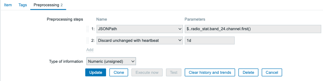
Within the Master item, we’re basically not parsing anything, it’s just there to receive the values and push them into the Dependent items. In the dependent items, we start “cherry-picking” only those metrics that we would like to see. As it’s JSON format, preprocessing step “JSONPath” comes in handy. At the same time, we’re looking into efficiency, so a second step is added: discard unchanged with heartbeat (1d):

Example: Getting out the statistics of the 2.4Ghz band radio:

Item prototype proprocessing

Of course, this has to be done with all items.

So far, we’ve heavily focussed on the technical part, but Zabbix does have quite a few options to visualize the data as well. As we’re waiting on the next LTS release, we have only set up a very small dashboard with a few widgets. One of the better ones:

number_clients

Here we’re using the new graph type widget, but instead of plotting the number of clients per AP, we’re plotting a dataset with an “aggregate” function. Of course, if we look at the dashboard widgets, there are many more things that can be visualized…

Efficiency and security considerations

As we were building this, we had 2 main considerations:

    • Efficiency
    • Security

Efficiency, as we are anticipating that Quanza will be responsible for quite a few MIST environments on top of the current environments in the near future, combined with a strict limit of allowed API calls against the MIST API. As such, it is really important to keep those API calls as low as possible. Next to that, with every new Access Point added, the load on the Zabbix server is increasing. Now that is not really a problem, as Zabbix is perfectly capable of monitoring thousands of metrics simultaneously, though it has its limits. And you do not want to hit those limits in a production environment with the only solution being migration to beefier hardware.

Security-wise this challenge had a few things going on since we’re talking to an external exposed API. MIST can invoke webhooks. This might’ve been a bit easier (we explored it, but there were of course other things to keep in mind while going down that road), but the main concern was the requirement that Zabbix / an interface to Zabbix is exposed to the internet. That didn’t look too appealing and required a bit more maintenance. The preferable solution was to create that middleware where we have full control of what queries are executed, how the API token is protected, which connections are established etc. etc.

Conclusion

Although this question was challenging, together with Quanza we created a scalable, secure, and dynamic solution. Zabbix is flexible enough to facilitate the tricks required to provide reliable monitoring and alerting in an efficient and secure manner. We strongly believe the only limitation is your own creativity and this case proves that once again.

Quanza can now ensure the availability of their customer Juniper MIST-based networks, and in case something breaks their 24×7 manned NOC will be able to take whatever action is required to ensure the availability of the customers’ network – all thanks to the flexibility of Zabbix.

The post Monitoring Juniper Mist wireless network appeared first on Zabbix Blog.

ZABBIX – Open-Source Monitoring Software for Automotive Monitoring

Post Syndicated from Dmitry Lambert original https://blog.zabbix.com/zabbix-open-source-monitoring-software-for-automotive-monitoring/18776/

In this article, I will try to cover the theoretical models on monitoring your vehicle fleet with minimal to no cost at all by using the ELM327 microcontroller, a python library to process the collected data and a Zabbix proxy running on a small Raspberry Pi device to store and sent the collected metrics to the central Zabbix server.

Expanding the scope of our Zabbix instance

The first thing that comes to mind when someone mentions a monitoring system is pretty simple. People think about server monitoring, and with servers, we usually mean Linux and Windows systems and also network monitoring for all kinds of flavors of switches, routers, firewalls, etc. But by putting so much focus on these standard things, we are someway limiting the possibilities of monitoring systems. Zabbix has proven itself as an extremely powerful monitoring tool that can combine and monitor all client infrastructure – no matter if we are talking about the aforementioned servers, network devices, services, applications, or anything else. And most important – Zabbix is truly a 100% open-source product, which allows anyone to use all listed functionalities for free.

Please, keep in mind that no doubt there are systems available that are created exactly for the same purpose I will cover here. Maybe they are more reliable. Perhaps they require less effort to achieve the desired result. But that is the exact reason why the presented model is mostly theoretical, with the primary goal being to show that it is hard to put Zabbix in some functionality boundaries. Usually, the only limitation is our imagination. And it is up to you to treat this information for pure entertainment or try to implement it in a place where you find it suitable.

Monitoring a car fleet

Let’s get straight to the point. You don’t need to own a huge logistics company with a thousand vehicle fleet to understand it. In simple words – if you or any of your relatives own a car, you should be aware that cars tend to break. Just like it usually happens, there could be many types of issues, starting with a flat tire and ending with some ongoing damage in the gearbox or engine. It is important to understand that vehicles themselves are becoming smarter. If in the past it was a purely mechanical device, then nowadays it is a highly complicated electronic system on top of that mechanical device that can diagnose the slightest deviations from accepted norms that are set by the manufacturer and inform about this malfunction either with an indicator light on your dash or simply with a log message that will be accessible only when read with specialized software or tools.

No alt text provided for this image


Keep in mind that malfunctions in vehicles are not as simple as boolean ( works or not ). In most cases an issue is noticed before the car is not able to move forward, and the purpose of that is to be informed and fix the issue before it has turned into a defect that actually prevents the vehicle from functioning.

And now think about this from an automotive business perspective. We may be talking about hundreds of vehicles that are always on the move to deliver something or someone in time. It should be straightforward that in such a niche business, each of these vehicles should be able to traverse close to a thousand kilometers per day.

No alt text provided for this image


Thankfully, as mentioned previously, the smart diagnostic system will let you know about all the potential problems. On the other hand, the driver of the vehicle usually has nothing to do with its repairs or technical condition. So in a perfect world, we should have a few technical employees that would simply ask returning driver whether everything is fine with the car after his shift – are there any errors, and connect with diagnostic software to read its logs to make sure that everything actually is ok. If it’s not ok, information should be passed to the technical department to move this vehicle to the maintenance.

Why such pressure? Well, remember that most of these notifications serve as a warning that something is not working as it should, but currently, it is not causing harm. However, if it is ignored, there is a high chance that at some point, the vehicle will not be able to continue its way to the destination.

No alt text provided for this image


So this is where Zabbix joins the conversation. Imagine if all this data transfer from the vehicle diagnostic system to the responsible employees would happen automatically, with potential error prioritization and escalation to further levels if any vehicle has an ongoing issue that remains active for multiple days. And remember that Zabbix is a completely free and open-source system, which means that we could achieve this result for free. And we are absolutely not limited to DTC ( Diagnostic Trouble Codes ) readings. Combining this ecosystem with the recent Zabbix 6.0 LTS release, we can create a geomap with the current location of any vehicle from our fleet. With a little effort, we can also get speed measurements, long stops, starts, and much more.

This is the part when the tested but still theoretical model comes into action. By now, we are aware that a car is way smarter than it may look, and it gathers and stores a lot of useful information. However, the Zabbix monitoring system as per the most common standard sits somewhere in our headquarters and monitors generic metrics of our IT infrastructure. So how could we potentially get this information from our vehicle to Zabbix?

No alt text provided for this image


Since all information is stored in ECU (Electronic Control Unit), there is also a way to read it. And it is achieved through OBD (On-Board Diagnostic) socket through the standardized protocol. Just like anything else, OBD has multiple versions or protocols of communications. Still, if we are talking about seamlessly modern cars, most likely we are talking about OBD-II, which included Electronic signaling and messaging format.

Using ELM327 to gather data

precisely OBD-II will help us to gather all information from the vehicle, to further transfer it to our Zabbix monitoring system. Initially, this may yet sound very unclear because we have some kind of socket to access our ECU, but how can we actually gather some meaningful data? For that, we will need ELM327

No alt text provided for this image


ELM327 is a programmed microcontroller produced by ELM Electronics for translating the OBD interface. Even today ELM327 command protocol is one of the most popular PC to OBD interface standards. Typically ELM abstracts the low-level protocol and presents a simple interface that can be called via UART, typically by a hand-held diagnostic tool or a computer program connected by USB, RS-232, Bluetooth, or WiFi. In our case, we don’t need and don’t have any dedicated diagnostic tool, so we will have to use something else to work with OBD-II and translate all incoming data. With the ELM-327, it is straightforward. You can purchase an ELM327 OBD2-Bluetooth adapter on Amazon for a couple of dollars, and it will be enough to provide the required functionality.

No alt text provided for this image

Data processing with Python-OBD and Raspberry Pi

As it usually happens, for all things that we need, we can find a Python library published under GPLv2. And as you already noticed from the screenshot, we are not limited to stored DTC values. In addition to that, we are able to read live data from our vehicle, such as speed, fuel pressure, coolant temperature, intake temperature, and much more.

No alt text provided for this image


The closer we get to the result, the simpler the task starts to look. At this point, we basically have everything that we need. We have the data, and we have the interface from which to read it. ELM327 allows us to transport this data to our device, and the python library will enable us to translate and process this information, therefore allowing sending clean data to our Zabbix. The only open question is what device should we use in our vehicle, on which we could run our Python script, and which would have GSM access to transfer gathered data to the Zabbix server. In my example choice was as simple as cheap – Raspberry Pi.

No alt text provided for this image


And then it’s a matter of choice when you have Raspberry set up on a vehicle, connected via Bluetooth or any other way to your ELM327, that is plugged into an OBD-II connector. With Python script running on Pi device to receive and process data from our ECM, we need to decide what piece of software from Zabbix we want on this device.

Zabbix proxy for data storage

Considering that the car could be driving through different areas where internet coverage could not be the best, but we also don’t want to lose any data simply because there was no connection, I think it is best to install Zabbix proxy on Raspberry Pi.

Zabbix proxy perfectly suits such a small setup and helps us with its main purpose. Proxy has a local database that stores all information that has to be sent to our Zabbix server. If because of some networking trouble this data can’t be passed to our server, it will be kept in the local database for a moment when a network connection is restored and data is sent. Luckily for us, Zabbix has Official Packages for Raspberry Pi OS, so we don’t need to tailor any magic around it.

The functionality of the Zabbix proxy allows us to choose between two modes ( Active and Passive ), which basically allows us to choose the direction of communication. It might not be the cheapest approach to purchase a static IP address for each unit. Therefore we will be using Zabbix Proxy (Active), which simply will connect to our Zabbix server and send all gathered information. Of course, there are security measures for validation to make sure that only designated devices will be able to send data to a server. If an even more secure approach is required, users may choose to use TLS encryption with PSK or Certificates.

No alt text provided for this image

Collecting the current latitude and longitude

Previously I mentioned, that with the new Geomap widget, it is possible to achieve a live view of the current location from all your fleet on a single dashboard. To do that, we obviously need live latitude and longitude readings, which ECU and stock Raspberry Pi are not able to provide. But this is the beauty of Raspberry Pi. With minimal investments, we can purchase a GPS unit and combine it with our Pi.

No alt text provided for this image

With a very simplified Python script, we can gather all required data, and move it to our Zabbix proxy that is installed on localhost, which then will parse this information to our Zabbix Server that will allow us to see it in the dashboard. As this is not a very native and straightforward approach to monitoring, we won’t be able to use native item types to collect this data. This means that all the collection must be done within the script, and then we need to pass this data using the Zabbix-sender utility. The purpose of this utility is very simple, without any complications, take data that is provided and send it to a specified Hostname.

No alt text provided for this image


Since Zabbix has a very powerful preprocessing engine, we don’t have to make our script over-complicated with data transformation to meet guidelines for data visualization within Zabbix. We can send raw data, just like it is, and then use any suitable preprocessing step in the Zabbix frontend to extract the value we need to visualize.

No alt text provided for this image

The many uses of the collected data

When the data arrives in the Latest data in our Zabbix frontend, consider the most complicated part of this task is done. And just like before the idea of automotive monitoring with Zabbix, the only limitation is your imagination. You can simply collect this data without any actions. Monitor it on your own, from time to time, just to see if you can do anything meaningful with it.

You are also able to utilize a wide list of trigger functions within Zabbix to define that it is a problem when some particular value is received. For example, when some DTC appeared on a device, or let’s say, the average speed of the vehicle exceeds a threshold. Maybe you want to set some borders for coordinates, and if a particular vehicle gets outside of a specified radius, it could raise a problem in your monitoring system.

It is up to you how to react to these triggers. It could be just a flashing light on your Problems view within the Zabbix frontend. It could also automatically create incidents for your maintenance team with a message that a particular vehicle has worn out brake pads that has to be replaced. But maybe if these brake pads are not replaced for a full week since the first time it was noticed, you want to receive a personalized message on your mobile phone so that you can escalate this issue further.

No secret that there are flaws and downsides. As I mentioned right in beginning, there are software and devices that are developed and adopted exactly for this purpose, however, my approach may not be 100% reliable. Data transfer from ECU is not as live as reading CPU utilization from your computer. All of this is just a reminder that monitoring is not limited to network devices and servers. And Zabbix, which is growing every year, provides more and more features to its users while remaining absolutely free and open-source, is here to support all your ideas and help them come to life.

The post ZABBIX – Open-Source Monitoring Software for Automotive Monitoring appeared first on Zabbix Blog.

How Belcorp decreased cost and improved reliability in its big data processing framework using Amazon EMR managed scaling

Post Syndicated from Diego Benavides original https://aws.amazon.com/blogs/big-data/how-belcorp-decreased-cost-and-improved-reliability-in-its-big-data-processing-framework-using-amazon-emr-managed-scaling/

This is a guest post by Diego Benavides and Luis Bendezú, Senior Data Architects, Data Architecture Direction at Belcorp.

Belcorp is one of the main consumer packaged goods (CPG) companies providing cosmetics products in the region for more than 50 years, allocated to around 13 countries in North, Central, and South America (AMER). Born in Peru and with its own product factory in Colombia, Belcorp always stayed ahead of the curve and adapted its business model according to customer needs and strengthened its strategy with technological trends, providing each time a better customer experience. Focused on this, Belcorp began to implement its own data strategy encouraging the use of data for decision-making. Based on this strategy, the Belcorp data architecture team designed and implemented a data ecosystem allowing business and analytics teams to consume functional data that they use to generate hypotheses and insights that are materialized in better marketing strategies or novel products. This post aims to detail a series of continuous improvements carried out during 2021 in order to reduce the number of platform incidents reported at the end of 2020, optimize SLAs required by the business, and be more cost-efficient when using Amazon EMR, resulting in up to 30% savings for the company.

To stay ahead of the curve, stronger companies have built a data strategy that allows them to improve main business strategies, or even create new ones, using data as a main driver. As one of the main consumer packaged goods (CPG) companies in the region, Belcorp is not an exception—in recent years we have been working to implement data-driven decision-making.

We know that all good data strategy is aligned to business objectives and based on main business use cases. Currently, all our team efforts are focused on the final consumers, and almost all business initiatives are related to hyper-personalization, pricing, and customer engagement.

To support these initiatives, the data architecture department provides data services like data integration, only one source of truth, data governance and data quality frameworks, data availability, data accessibility, and optimized time to market, according to business requirements like other big companies. To provide minimal capabilities to support all these services, we needed a scalable, flexible, and cost-efficient data ecosystem. Belcorp started this adventure a couple of years ago using AWS services like Amazon Elastic Compute Cloud (Amazon EC2), AWS Lambda, AWS Fargate, Amazon EMR, Amazon DynamoDB, and Amazon Redshift, which currently feed our main analytical solutions with data.

As we were growing, we had to continually improve our architecture design and processing framework in regards to data volume and more complex data solution requirements. We also had to adopt quality and monitoring frameworks in order to guarantee data integrity, data quality, and service level agreements (SLAs). As you can expect, it’s not an easy task, and requires its own strategy. At the beginning of 2021 and due to critical incidents we were finding, operational stability was affected, directly impacting business outcomes. Billing was also impacted, due to more new complex workloads being included, which caused an unexpected increase in platform costs. In response, we decided to focus on three challenges:

  • Operational stability
  • Cost-efficiency
  • Service level agreements

This post details some action points we carried out during 2021 over Belcorp’s data processing framework based on Amazon EMR. We also discuss how these actions helped us face the challenges previously mentioned, and also provide economic savings to Belcorp, which was the data architecture team’s main contribution to the company.

Overview of solution

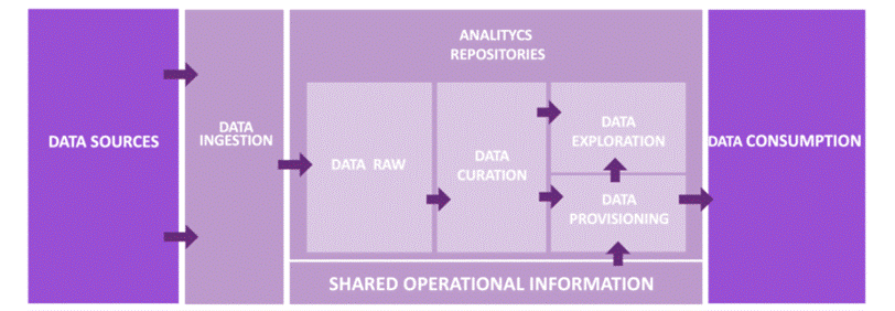
Belcorp’s data ecosystem is composed by seven key capability pillars (as shown in the following diagram) that define our architectural design and give us more or less technological flexible options. Our data platform can be classified as a part of the second generation of data platforms, as mentioned by Zhamak Dehghani in How to Move Beyond a Monolithic Data Lake to a Distributed Data Mesh. In fact, it has all the limitations and restrictions of a Lakehouse approach as mentioned in the paper Lakehouse: A New Generation of Open Platforms that Unify Data Warehousing and Advanced Analytics .

Belcorp’s data platform supports two main use cases. On one side, it provides data to be consumed using visualization tools, encouraging self-service. On the other side, it provides functional data to end-users, like data scientists or data analysts, through distributed data warehouses and object storage more suited to advanced analytical practices.

The following reference design explains the main two layers in charge of providing functional data for these use cases. The data processing layer is composed of two sub-layers. The first is Belcorp’s Data Lake Integrator, which is a built-in, in-house Python solution with a set of API REST services in charge of organizing all the data workloads and data stages inside the analytics repositories. It also works as a point of control to distribute resources to be allocated for each Amazon EMR Spark job. The processing sub-layer is mainly composed of the EMR cluster, which is in charge of orchestrating, tracking, and maintaining all the Spark jobs developed using a Scala framework.

For the persistent repository layer, we use Amazon Simple Storage Service (Amazon S3) object storage as a data repository for analytics workloads, where we have designed a set of data stages that have operational and functional purposes based on the reference architecture design. Discussing the repository design in more depth is out of scope for this post, but we must note that it covers all the common challenges related to data availability, data accessibility, data consistency, and data quality. In addition, it achieves all Belcorp’s needs required by its business model, despite all limitations and restrictions we inherit by the design previously mentioned.

We can now move our attention to the main purpose of this post.

As we mentioned, we experienced critical incidents (some of which existed before) and unexpected cost increases at the beginning of 2021, which motivated us to take action. The following table lists some of the main issues that attracted our attention.

Reported Incidents Impact
Delay in Spark jobs on Amazon EMR Core workloads take a long time
Delay in Amazon EMR nodes auto scaling Workloads take a long time
Increase in Amazon EMR computational usage per node Unexpected cost increase
Lost resource containers Workloads process a huge data crash
Overestimated memory and CPUs Unexpected cost increase

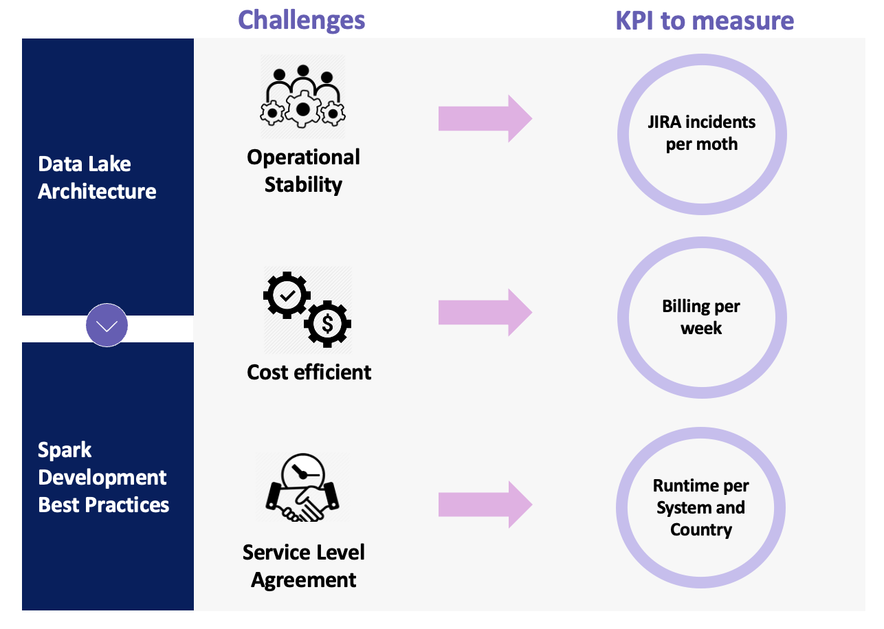
To face these issues, we decided to change strategies and started to analyze each issue in order to identify the cause. We defined two action lines based on three challenges that the leaders wanted us to work on. The following figure summarizes these lines and challenges.

The data lake architecture action line refers to all the architectural gaps and deprecated features that we determined as part of the main problems that were generating the incidents. The Spark development best practices action line is related to the developed Spark data solution that had been causing instability due to bad practices during the development lifecycle. Focusing on these action lines, our leaders defined three challenges in order to decrease the number of incidents and guarantee the quality of the service we provide: operational stability, cost-efficiency, and SLAs.

Based on these challenges, we defined three KPIs to measure the success of the project. Jira incidents allow us to validate that our changes are having a positive impact; billing per week shows the leaders that part of the changes we applied will gradually optimize cost; and runtime provides the business users with a better time to market.

Next, we defined the next steps and how to measure progress. Based on our monitoring framework, we determined that almost all incidents that arose were related to the data processing and persistent repository layers. Then we had to decide how to solve them. We could make reactive fixes in order to achieve operational stability and not have an impact on business, or we could change our usual way of working, analyze each issue, and provide a final solution to optimize our framework. As you can guess, we decided to change our way of working.

We performed a preliminary analysis to determine the main impacts and challenges. We then proposed the following actions and improvements based on our action lines:

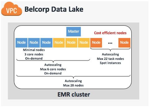
  • Data lake architecture – We redesigned the EMR cluster; we’re now using core and task nodes
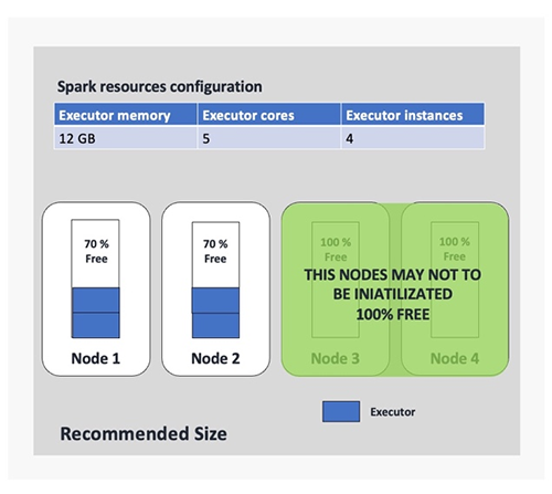
  • Spark development best practices – We optimized Spark parameters (RAM memory, cores, CPUs, and executor number)

In the next section, we explain in detail the actions and improvements proposed in order to achieve our goals.

Actions and improvements

As we mentioned in the previous section, the analysis made by the architecture team resulted in a list of actions and improvements that would help us face three challenges: operational stability, a cost-efficient data ecosystem, and SLAs.

Before going further, it’s a good time to provide more details about the Belcorp data processing framework. We built it based on Apache Spark using the Scala programming language. Our data processing framework is a set of scalable, parameterizable, and reusable Scala artifacts that provide development teams with a powerful tool to implement complex data pipelines, achieving the most complex business requirements using Apache Spark technology. Through the Belcorp DevOps framework, we deploy each artifact to several non-production environments. Then we promote into production, where the EMR cluster launches all the routines using the Scala artifacts that reference each conceptual area inside the analytical platform. This part of the cycle provides the teams with some degree of flexibility and agility. However, we forgot, for a moment, the quality of the software we were developing using Apache Spark technology.

In this section, we dive into the actions and improvements we applied in order to optimize the Belcorp data processing framework and improve the architecture.

Redesigning the EMR cluster

The current design and implementation of the Belcorp data lake is not the first version. We’re currently in version 2.0, and from the beginning of the first implementation until now, we’ve tried different EMR cluster designs to implement the data processing layer. Initially, we used a fixed cluster with four nodes (as shown in the following figure), but when the auto scaling capability was launched and Belcorp’s data workloads increased, we decided to move it there to optimize resource usage and costs. However, an auto scaled EMR cluster has different options too. You can choose between core and task nodes with a minimal and maximum number of each. In addition, you can select On-Demand or Spot Instances. You can also implement an optimized allocation strategy using EMR instance fleets to reduce the probability of Spot Instance loss. For more information about Amazon EMR resources allocation strategies, see Spark enhancements for elasticity and resiliency on Amazon EMR and Optimizing Amazon EMR for resilience and cost with capacity-optimized Spot Instances.

We tested all these capabilities, but we found some problems.

First, although AWS offers many capabilities and functionalities around Amazon EMR, if you don’t have some degree of knowledge about the technology that you want to use, you may encounter many issues as the use cases arise. As we mentioned, we decided to use the Apache Spark data processing engine through Amazon EMR as a part of Belcorp data ecosystem, but we faced many issues. Whenever an incident appeared, it motivated the data architect team in charge to fix it, as a part of the operational and support tasks. Almost all these reactive fixes were related to changing Amazon EMR configuration to try different alternatives in order to efficiently solve these incidents.

We figured out that almost all incidents were related to resource allocation, so we tested many configuration options such as instance types, increasing the number of nodes, customized rules for auto scaling, and fleet strategies. This last option was used to reduce node loss. At the end of 2020, we validated that an EMR cluster with automatic scaling enabled with a minimum capacity of three On-Demand core nodes 24/7 and the ability to scale up to 25 On-Demand core nodes provided us with a stable data processing platform. At the beginning of 2021, more complex Spark jobs were deployed as a part of the data processing routines inside the EMR cluster, causing operational instability again. In addition, the billing was increasing unexpectedly, which alerted leaders whose team needed to redesign the EMR cluster in order to keep healthy operational stability and optimize the costs.

We soon realized that it was possible to reduce up to 40% of the current billing using Spot Instances, instead of keeping all core nodes in On-Demand consumption. Another infrastructure optimization that we wanted to apply was to replace a number of core nodes with task nodes, because almost all Belcorp data workloads are memory-intensive and use Amazon S3 to read the source data and write the result dataset. The question here was how to do that without losing the benefits of the current design. To answer this question, we had the guidance of the AWS Account Team and our AWS Analytics and Big Data Specialist SA, in order to clarify questions about the following:

  • Apache Spark implementation in Amazon EMR
  • Core and task node best practices for production environments
  • Spot Instance behavior in Amazon EMR

We definitely recommend addressing these three main points before applying any changes because, according to our previous experience, making modifications in the dark can lead to costly and underperforming Amazon EMR implementation. With that in mind, we redesigned the EMR cluster to utilize EMR managed scaling, which automatically resizes your cluster for best performance at the lowest possible cost. We defined a maximum of 28 capacity units with three On-Demand core nodes always on (24/7) in order to support data workloads during the day. We then set an auto scaling limit of six On-Demand cores in order to provide minimal HDFS capabilities to support the remaining 22 task nodes composed of Spot Instances. This final configuration is based on advice from AWS experts that we have at least one core node to support six task nodes, keeping a 1:6 ratio. The following table summarizes our cluster design.

Cluster Scaling Policy Amazon EMR Managed Scaling Enabled
Minimum node units (MinimumCapacityUnits) 3
Maximum node units (a) 28
On-demand limit (MaximumOnDemandCapacityUnits) 6
Maximum core nodes (MaximumCoreCapacityUnits) 6
Instance type m4.10xlarge
Number of primary nodes 1
Primary node instance type m4.4xlarge

The following figure illustrates our updated and current cluster design.

Tuning Spark parameters

As any good book about Apache Spark can tell you, Spark parameter tuning is the main topic you need to look into before deploying a Spark application in production.

Adjusting Spark parameters is the task of setting up the resources (CPUs, memory, and the number of executors) to each Spark application. In this post, we don’t focus on driver instance resources; we focus on the executors because that’s the main issue we found inside Belcorp’s implementation.

After we applied improvements around join operation and cache strategies in Spark application development, we realized that some of those applications were assigned with overestimated resources in the EMR cluster. That means Spark applications assigned resources, but only 30% of the resources were used. The following Ganglia report illustrates the overestimation of resource allocation for one Spark application job, which we captured during one of our tests.

A big consequence of this behavior was the massive deployment of EMR nodes that weren’t being properly utilized. That means that numerous nodes were provisioned because of the auto scaling feature required by a Spark application submit, but much of the resources of these nodes were kept free. We show a basic example of this later in this section.

With this evidence, we began to suspect that we needed to adjust the Spark parameters of some of our Spark applications.

As we mentioned in previous sections, as part of the Belcorp data ecosystem, we built a Data Pipelines Integrator, which has the main responsibility of maintaining centralized control of the runs of each Spark application. To do that, it uses a JSON file containing the Spark parameter configuration and performs each spark-submit using Livy service, as shown in the following example code:

'/usr/lib/spark/bin/spark-submit' '--class' 'LoadToFunctional' '--conf' 'spark.executor.instances=62' '--conf' 'spark.executor.memory=17g' '--conf' 'spark.yarn.maxAppAttempts=2' '--conf' 'spark.submit.deployMode=cluster' '--conf' 'spark.master=yarn' '--conf' 'spark.executor.cores=5' 's3://<bucket-name>/FunctionalLayer.jar' '--system' 'CM' '--country' 'PE' '--current_step' 'functional' '--attempts' '1' '--ingest_attributes' '{"FileFormat": "zip", "environment": "PRD", "request_origin": "datalake_integrator", "next_step": "load-redshift"}' '--fileFormat' 'zip' '--next_step' 'load-redshift'

This JSON file contains the Spark parameter configuration of each Spark application related to an internal system and country we submit to the EMR cluster. In the following example, CM is the name of the system and PE is the country code that the data comes from:

"systems" : {
  "CM" : {
    "PE" : { 
      "params" : {"executorCores": 15, "executorMemory": "45g", "numExecutors": 50 },
      "conf" : { "spark.sql.shuffle.partitions" :120 }
    }
}

The problem with this approach is that as we add more applications, the management of these configuration files becomes more complex. In addition, we had a lot of Spark applications set up with a default configuration that was defined a long time ago when workloads were less expensive. So, it was expected that some things would change. One example of a Spark application with uncalibrated parameters is shown in the following figure (we use four executor instances only for the example). In this example, we realized we were allocating executors with a lot of resources without following any of the Spark best practices. This was causing the provisioning of fat executors (using Spark slang) allocating each of those in at least one node. That means that if we define a Spark application to be submitted using 10 executors, we require at least 10 nodes of the cluster and use 10 nodes for only one run, which was very expensive for us.

When you deal with Spark parameter tuning challenges, it’s always a good idea to follow expert advice. Perhaps one of the most important pieces of advice is related to the number of executor cores you should use in one Spark application. Experts suggest that an executor should have up to four or five cores. We were familiar with this restriction because we formerly developed Spark applications in the Hadoop ecosystem because of Hadoop File Systems I/O restrictions. That is, if we have more cores configured for one executor, we perform more I/O operations in a single HDFS data node, and it’s well known that HDFS degrades due to high concurrency. This constraint isn’t a problem if we use Amazon S3 as storage, but the suggestion remains due to the overload of the JVM. Remember, while you have more operational tasks, like I/O operations, the JVM of each executor has more work to do, so the JVM is degraded.

With these facts and previous findings, we realized that for some of our Spark applications, we were using only 30% of the assigned resources. We needed to recalibrate the Spark job parameters in order to allocate only the best-suited resources and significantly reduce the overuse of EMR nodes. The following figure provides an example of the benefits of this improvement, where we can observe a 50% of node reduction based on our earlier configuration.

We used the following optimized parameters to optimize the Spark application related to the CM system:

"systems" : {
  "CM" : {
    "PE" : { 
      "params" : {"executorCores": 5, "executorMemory": "17g", "numExecutors": 62 },
      "conf" : { "spark.sql.shuffle.partitions" :120 }
    }
}

Results

In this post, we wanted to share the success story of our project to improve the Belcorp data ecosystem, based on two lines of actions and three challenges defined by leaders using AWS data technologies and in-house platforms.

We were clear about our objectives from the beginning based on the defined KPIs, so we’ve been able to validate that the number of JIRA incidents reported at the end of May 2021 had a notable reduction. The following figures shows a reduction of up to 75% in respect to previous months, highlighting March as a critical peak.

Based on this incident reduction, we figured out that almost all Spark job routines running in the EMR cluster benefitted from a runtime optimization, including the two most complex Spark jobs, with a reduction up to 60%, as shown in the following figure.

Perhaps the most important contribution of the improvements made by the team is directly related to the billing per week. For example, Amazon EMR redesigning, the join operation improvements, cache best practices applied, and Spark parameter tuning—all of these produced a notable reduction in the use of cluster resources. As we know, Amazon EMR calculates billing based on the time that the cluster nodes have been on, regardless of whether they do any work. So, when we optimized EMR cluster usage, we optimized the costs we were generating as well. As shown in the following figure, only in 2 months, between March and May, we achieved a billing reduction of up to 40%. We estimate that we will save up to 26% of the annual billing that would have been generated without the improvements.

Conclusion and next steps

The data architecture team is in charge of the Belcorp data ecosystem’s continuous improvements, and we’re always being challenged to achieve a best-in-class architecture, craft better architectural solution designs, optimize cost, and create the most automated, flexible, and scalable frameworks.

At the same time, we’re thinking about the future of this data ecosystem—how we can adapt to new business needs, generate new business models, and address current architectural gaps. We’re working now on the next generation of the Belcorp data platform, based on novel approaches like data products, data mesh, and lake houses. We believe these new approaches and concepts are going to help us to cover our current architectural gaps in the second generation of our data platform design. Additionally, it’s going to help us better organize the business and development teams in order to obtain greater agility during the development cycle. We’re thinking of data solutions as a data product, and providing teams with a set of technological components and automated frameworks they can use as building blocks.

Acknowledgments

We would like to thank our leaders, especially Jose Israel Rico, Corporate Data Architecture Director, and Venkat Gopalan, Chief Technology, Data and Digital Officer, who inspire us to be customer centric, insist on the highest standards, and support every technical decision based on a stronger knowledge of the state of the art.


About the Authors

Diego Benavides is the Senior Data Architect of Belcorp in charge of the design, implementation, and the continuous improvement of the Global and Corporate Data Ecosystem Architecture. He has experience working with big data and advanced analytics technologies across many industry areas like telecommunication, banking, and retail.

Luis Bendezú works as a Senior Data Engineer at Belcorp. He’s in charge of continuous improvements and implementing new data lake features using a number of AWS services. He also has experience as a software engineer, designing APIs, integrating many platforms, decoupling applications, and automating manual jobs.

Mar Ortiz is a bioengineer who works as a Solutions Architect Associate at AWS. She has experience working with cloud compute and diverse technologies like media, databases, compute, and distributed architecture design.

Raúl Hugo is an AWS Sr. Solutions Architect with more than 12 years of experience in LATAM financial companies and global telco companies as a SysAdmin, DevOps engineer, and cloud specialist.
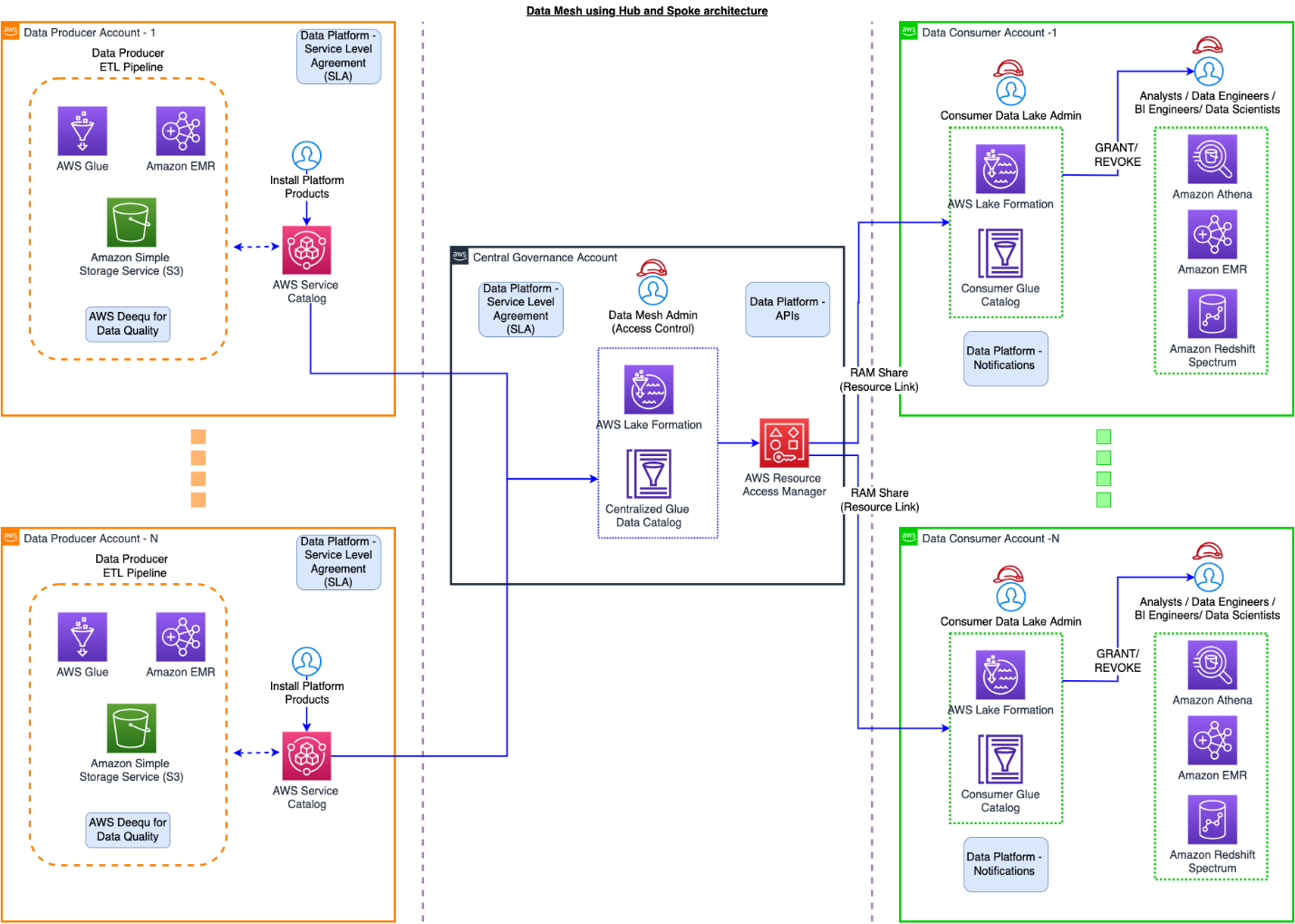
Ibotta builds a self-service data lake with AWS Glue

Post Syndicated from Erik Franco original https://aws.amazon.com/blogs/big-data/ibotta-builds-a-self-service-data-lake-with-aws-glue/

This is a guest post co-written by Erik Franco at Ibotta.

Ibotta is a free cash back rewards and payments app that gives consumers real cash for everyday purchases when they shop and pay through the app. Ibotta provides thousands of ways for consumers to earn cash on their purchases by partnering with more than 1,500 brands and retailers.

At Ibotta, we process terabytes of data every day. Our vision is to allow for these datasets to be easily used by data scientists, decision-makers, machine learning engineers, and business intelligence analysts to provide business insights and continually improve the consumer and saver experience. This strategy of data democratization has proven to be a key pillar in the explosive growth Ibotta has experienced in recent years.

This growth has also led us to rethink and rebuild our internal technology stacks. For example, as our datasets began to double in size every year combined with complex, nested JSON data structures, it became apparent that our data warehouse was no longer meeting the needs of our analytics teams. To solve this, Ibotta adopted a data lake solution. The data lake proved to be a huge success because it was a scalable, cost-effective solution that continued to fulfill the mission of data democratization.

The rapid growth that was the impetus for the transition to a data lake has now also forced upstream engineers to transition away from the monolith architecture to a microservice architecture. We now use event-driven microservices to build fault-tolerant and scalable systems that can react to events as they occur. For example, we have a microservice in charge of payments. Whenever a payment occurs, the service emits a PaymentCompleted event. Other services may listen to these PaymentCompleted events to trigger other actions, such as sending a thank you email.

In this post, we share how Ibotta built a self-service data lake using AWS Glue. AWS Glue is a serverless data integration service that makes it easy to discover, prepare, and combine data for analytics, machine learning, and application development.

Challenge: Fitting flexible, semi-structured schemas into relational schemas

The move to an event-driven architecture, while highly valuable, presented several challenges. Our analytics teams use these events for use cases where low-latency access to real-time data is expected, such as fraud detection. These real-time systems have fostered a new area of growth for Ibotta and complement well with our existing batch-based data lake architecture. However, this change presented two challenges:

  • Our events are semi-structured and deeply nested JSON objects that don’t translate well to relational schemas. Events are also flexible in nature. This flexibility allows our upstream engineering teams to make changes as needed and thereby allows Ibotta to move quickly in order to capitalize on market opportunities. Unfortunately, this flexibility makes it very difficult to keep schemas up to date.
  • Adding to these challenges, in the last 3 years, our analytics and platform engineering teams have doubled in size. Our data processing team, however, has stayed the same size largely due to difficulty in hiring qualified data engineers who possess specialized skills in developing scalable pipelines and industry demand. This meant that our data processing team couldn’t keep up with the requests from our analytics teams to onboard new data sources.

Solution: A self-service data lake

To solve these issues, we decided that it wasn’t enough for the data lake to provide self-service data consumption features. We also needed self-service data pipelines. These would provide both the platform engineering and analytics teams with a path to make their data available within the data lake and with minimal to no data engineering intervention necessary. The following diagram illustrates our self-service data ingestion pipeline.

The pipeline includes the following components:

  1. Ibotta data stakeholders – Our internal data stakeholders wanted the capability to automatically onboard datasets. This user base includes platform engineers, data scientists, and business analysts.
  2. Configuration file – Our data stakeholders update a YAML file with specific details on what dataset they need to onboard. Sources for these datasets include our enterprise microservices.
  3. Ibotta enterprise microservices – Microservices make up the bulk of our Ibotta platform. Many of these microservices utilize events to asynchronously communicate important information. These events are also valuable for deriving analytics insights.
  4. Amazon Kinesis – After the configuration file is updated, data is immediately streamed to Amazon Kinesis. Amazon Kinesis makes it easy to collect, process, and analyze real-time, streaming data so you can get timely insights and react quickly to new information. Streaming the data through Kinesis Data Streams and Kinesis Data Firehose gives us the flexibility to analyze the data in real time while also allowing us to store the data in Amazon Simple Storage Service (Amazon S3).
  5. Ibotta self-service data pipeline – This is the starting point of our data processing. We use Apache Airflow to orchestrate our pipelines once every hour.
  6. Amazon S3 raw data – Our data lands in Amazon S3 without any transformation. The complex nature of the JSON is retained for future processing or validation.
  7. AWS Glue – Our goal now is to take the complex nested JSON and create a simpler structure. AWS Glue provides a set of built-in transforms that we use to process this data. One of the transforms is Relationalize—an AWS Glue transform that takes semi-structured data and transforms it into a format that can be more easily analyzed by engines like Presto. This feature means that our analytics teams can continue to use the analytics engines they’re comfortable with and thereby lessen the impact of transitioning from relational data sources to semi-structured event data sources. The Relationalize function can flatten nested structures and create multiple dynamic frames. We use 80 lines of code to convert any JSON-based microservice message to a consumable table. We have provided this code base here as a reference and not for reuse.
    // Convert to a DynamicFrame and relationalize
       // Convert it back to DataFrame
       val dynamicFrame: DynamicFrame = DynamicFrame(df, glueContext)
       val dynamicFrameCollection: Seq[DynamicFrame] = dynamicFrame.relationalize(rootTableName = glueSourceTable,
         stagingPath = glueTempStorage,
         options = JsonOptions.empty)
       val relationalizedDF: Dataset[Row] = removeColumnDotNotationRelationalize(dynamicFrameCollection(0).toDF())
       // Get rid of dot-notation and repartition it
       val repartitionedDF: Dataset[Row] = relationalizedDF.repartition(finalRepartitionValue.toInt)
       // Write it out
       repartitionedDF
         .write
         .mode("overwrite")
         .option("compression", "snappy")
         .parquet(glueRelationalizeOutputS3Path)

  8. Amazon S3 curated – We then store the relationalized structures as Parquet format in Amazon S3.
  9. AWS Glue crawler AWS Glue crawlers allow us to automatically discover schema and catalogs in the AWS Glue Data Catalog. This feature is a core component of our self-service data pipelines because it removes the requirement of having a data engineer manually create or update the schemas. Previously, if a change needed to occur, it flowed through a communication path that included platform engineers, data engineers, and analytics. AWS Glue crawlers effectively remove the data engineers from this communication path. This means new datasets or changes to datasets are made available quickly within the data lake. It also frees up our data engineers to continue working on improvements to our self-service data pipelines and other data paved roadmap features.
  10. AWS Glue Data Catalog – A common problem in growing data lakes is that the datasets can become harder and harder to work with. A common reason for this is a lack of discoverability of data within the data lake as well as a lack of clear understanding of what the datasets are conveying. The AWS Glue Catalog is a feature that works in conjunction with AWS Glue crawlers to provide data lake users with searchable metadata for different data lake datasets. As AWS Glue crawlers discover new datasets or updates, they’re recorded into the Data Catalog. You can then add descriptions at the table or fields levels for these datasets. This cuts down on the level of tribal knowledge that exists between various data lake consumers and makes it easy for these users to self-serve from the data lake.
  11. End-user data consumption – The end-users are the same as our internal stakeholders called out in Step 1.

Benefits

The AWS Glue capabilities we described make it a core component of building our self-service data pipelines. When we initially adopted AWS Glue, we saw a three-fold decrease in our OPEX costs as compared to our previous data pipelines. This was further enhanced when AWS Glue moved to per-second billing. To date, AWS Glue has allowed us to realize a five-fold decrease in OPEX costs. Also, AWS Glue requires little to no manual intervention to ingest and process our over 200 complex JSON objects. This allows Ibotta to utilize AWS Glue each day as a key component in providing actionable data to the organization’s growing analytics and platform engineering teams.

We took away the following learnings in building self-service data platforms:

Conclusion and next steps

With the self-service data lake we have established, our business teams are realizing the benefits of speed and agility. As next steps, we’re going to improve our self-service pipeline with the following features:

  • AWS Glue streaming – Use AWS Glue streaming for real-time relationalization. With AWS Glue streaming, we can simplify our self-service pipelines by potentially getting rid of our orchestration layer while also getting data into the data lake sooner.
  • Support for ACID transactions – Implement data formats in the data lake that allow for ACID transactions. A benefit of this ACID layer is the ability to merge streaming data into data lake datasets.
  • Simplify data transport layers – Unify the data transport layers between the upstream platform engineering domains and the data domain. From the time we first implemented an event-driven architecture at Ibotta to today, AWS has offered new services such as Amazon EventBridge and Amazon Managed Streaming for Apache Kafka (Amazon MSK) that have the potential to simplify certain facets of our self-service and data pipelines.

We hope that this blog post will inspire your organization to build a self-service data lake using serverless technologies to accelerate your business goals.


About the Authors

Erik Franco is a Data Architect at Ibotta and is leading Ibotta’s implementation of its next-generation data platform. Erik enjoys fishing and is an avid hiker. You can often find him hiking one of the many trails in Colorado with his lovely wife Marlene and wonderful dog Sammy.

Shiv Narayanan is Global Business Development Manager for Data Lakes and Analytics solutions at AWS. He works with AWS customers across the globe to strategize, build, develop and deploy modern data platforms. Shiv loves music, travel, food and trying out new tech.

Matt Williams is a Senior Technical Account Manager for AWS Enterprise Support. He is passionate about guiding customers on their cloud journey and building innovative solutions for complex problems. In his spare time, Matt enjoys experimenting with technology, all things outdoors, and visiting new places.

How Goldman Sachs built persona tagging using Apache Flink on Amazon EMR

Post Syndicated from Balasubramanian Sakthivel original https://aws.amazon.com/blogs/big-data/how-goldman-sachs-built-persona-tagging-using-apache-flink-on-amazon-emr/

The Global Investment Research (GIR) division at Goldman Sachs is responsible for providing research and insights to the firm’s clients in the equity, fixed income, currency, and commodities markets. One of the long-standing goals of the GIR team is to deliver a personalized experience and relevant research content to their research users. Previously, in order to customize the user experience for their various types of clients, GIR offered a few distinct editions of their research site that were provided to users based on broad criteria. However, GIR did not have any way to create a personally curated content flow at the individual user level. To provide this functionality, GIR wanted to implement a system to actively filter the content that is recommended to their users on a per-user basis, keyed on characteristics such as the user’s job title or working region. Having this kind of system in place would both improve the user experience and simplify the workflows of GIR’s research users, by reducing the amount of time and effort required to find the research content that they need.

The first step towards achieving this is to directly classify GIR’s research users based on their profiles and readership. To that end, GIR created a system to tag users with personas. Each persona represents a type or classification that individual users can be tagged with, based on certain criteria. For example, GIR has a series of personas for classifying a user’s job title, and a user tagged with the “Chief Investment Officer” persona will have different research content highlighted and have a different site experience compared to one that is tagged with the “Corporate Treasurer” persona. This persona-tagging system can both efficiently carry out the data operations required for tagging users, as well as have new personas created as needed to fit use cases as they emerge.

In this post, we look at how GIR implemented this system using Amazon EMR.

Challenge

Given the number of contacts (i.e., millions) and the growing number of publications maintained in GIR’s research data store, creating a system for classifying users and recommending content is a scalability challenge. A newly created persona could potentially apply to almost every contact, in which case a tagging operation would need to be performed on several million data entries. In general, the number of contacts, the complexity of the data stored per contact, and the amount of criteria for personalization can only increase. To future-proof their workflow, GIR needed to ensure that their solution could handle the processing of large amounts of data as an expected and frequent case.

GIR’s business goal is to support two kinds of workflows for classification criteria: ad hoc and ongoing. An ad hoc criteria causes users that currently fit the defining criteria condition to immediately get tagged with the required persona, and is meant to facilitate the one-time tagging of specific contacts. On the other hand, an ongoing criteria is a continuous process that automatically tags users with a persona if a change to their attributes causes them to fit the criteria condition. The following diagram illustrates the desired personalization flow:

In the rest of this post, we focus on the design and implementation of GIR’s ad hoc workflow.

Apache Flink on Amazon EMR

To meet GIR’s scalability demands, they determined that Amazon EMR was the best fit for their use case, being a managed big data platform meant for processing large amounts of data using open source technologies such as Apache Flink. Although GIR evaluated a few other options that addressed their scalability concerns (such as AWS Glue), GIR chose Amazon EMR for its ease of integration into their existing systems and possibility to be adapted for both batch and streaming workflows.

Apache Flink is an open source big data distributed stream and batch processing engine that efficiently processes data from continuous events. Flink offers exactly-once guarantees, high throughput and low latency, and is suited for handling massive data streams. Also, Flink provides many easy-to-use APIs and mitigates the need for the programmer to worry about failures. However, building and maintaining a pipeline based on Flink comes with operational overhead and requires considerable expertise, in addition to provisioning physical resources.

Amazon EMR empowers users to create, operate, and scale big data environments such as Apache Flink quickly and cost-effectively. We can optimize costs by using Amazon EMR managed scaling to automatically increase or decrease the cluster nodes based on workload. In GIR’s use case, their users need to be able to trigger persona-tagging operations at any time, and require a predictable completion time for their jobs. For this, GIR decided to launch a long-running cluster, which allows multiple Flink jobs to be submitted simultaneously to the same cluster.

Ad hoc persona-tagging infrastructure and workflow

The following diagram illustrates the architecture of GIR’s ad hoc persona-tagging workflow on the AWS Cloud.

This is a broad overview, and the specifics of networking and security between components are out of scope for this post.

At a high level, we can discuss GIR’s workflow in four parts:

  1. Upload the Flink job artifacts to the EMR cluster.
  2. Trigger the Flink job.
  3. Within the Flink job, transform and then store user data.
  4. Continuous monitoring.

You can interact with Flink on Amazon EMR via the Amazon EMR console or the AWS Command Line Interface (AWS CLI). After launching the cluster, GIR used the Flink API to interact with and submit work to the Flink application. The Flink API provided a bit more functionality and was much easier to invoke from an AWS Lambda application.

The end goal of the setup is to have a pipeline where GIR’s internal users can freely make requests to update contact data (which in this use case is tagging or untagging contacts with various personas), and then have the updated contact data uploaded back to the GIR contact store.

Upload the Flink job artifacts to Amazon EMR

GIR has a GitLab project on-premises for managing the contents of their Flink job. To trigger the first part of their workflow and deploy a new version of the Flink job onto the cluster, a GitLab pipeline is run that first creates a .zip file containing the Flink job JAR file, properties, and config files.

The preceding diagram depicts the sequence of events that occurs in the job upload:

  1. The GitLab pipeline is manually triggered when a new Flink job should be uploaded. This transfers the .zip file containing the Flink job to an Amazon Simple Storage Service (Amazon S3) bucket on the GIR AWS account, labeled as “S3 Deployment artifacts”.
  2. A Lambda function (“Upload Lambda”) is triggered in response to the create event from Amazon S3.
  3. The function first uploads the Flink job JAR to the Amazon EMR Flink cluster, and retrieves the application ID for the Flink session.
  4. Finally, the function uploads the application properties file to a specific S3 bucket (“S3 Flink Job Properties”).

Trigger the Flink job

The second part of the workflow handles the submission of the actual Flink job to the cluster when job requests are generated. GIR has a user-facing web app called Personalization Workbench that provides the UI for carrying out persona-tagging operations. Admins and internal Goldman Sachs users can construct requests to tag or untag contacts with personas via this web app. When a request is submitted, a data file is generated that contains the details of the request.

The steps of this workflow are as follows:

  1. Personalization Workstation submits the details of the job request to the Flink Data S3 bucket, labeled as “S3 Flink data”.
  2. A Lambda function (“Run Lambda”) is triggered in response to the create event from Amazon S3.
  3. The function first reads the job properties file uploaded in the previous step to get the Flink job ID.
  4. Finally, the function makes an API call to run the required Flink job.

Process data

Contact data is processed according to the persona-tagging requests, and the transformed data is then uploaded back to the GIR contact store.

The steps of this workflow are as follows:

  1. The Flink job first reads the application properties file that was uploaded as part of the first step.
  2. Next, it reads the data file from the second workflow that contains the contact and persona data to be updated. The job then carries out the processing for the tagging or untagging operation.
  3. The results are uploaded back to the GIR contact store.
  4. Finally, both successful and failed requests are written back to Amazon S3.

Continuous monitoring

The final part of the overall workflow involves continuous monitoring of the EMR cluster in order to ensure that GIR’s tagging workflow is stable and that the cluster is in a healthy state. To ensure that the highest level of security is maintained with their client data, GIR wanted to avoid unconstrained SSH access to their AWS resources. Being constrained from accessing the EMR cluster’s primary node directly via SSH meant that GIR initially had no visibility into the EMR primary node logs or the Flink web interface.

By default, Amazon EMR archives the log files stored on the primary node to Amazon S3 at 5-minute intervals. Because this pipeline serves as a central platform for processing many ad hoc persona-tagging requests at a time, it was crucial for GIR to build a proper continuous monitoring system that would allow them to promptly diagnose any issues with the cluster.

To accomplish this, GIR implemented two monitoring solutions:

  • GIR installed an Amazon CloudWatch agent onto every node of their EMR cluster via bootstrap actions. The CloudWatch agent collects and publishes Flink metrics to CloudWatch under a custom metric namespace, where they can be viewed on the CloudWatch console. GIR configured the CloudWatch agent configuration file to capture relevant metrics, such as CPU utilization and total running EMR instances. The result is an EMR cluster where metrics are emitted to CloudWatch at a much faster rate than waiting for periodic S3 log flushes.
  • They also enabled the Flink UI in read-only mode by fronting the cluster’s primary node with a network load balancer and establishing connectivity from the Goldman Sachs on-premises network. This change allowed GIR to gain direct visibility into the state of their running EMR cluster and in-progress jobs.

Observations, challenges faced, and lessons learned

The personalization effort marked the first-time adoption of Amazon EMR within GIR. To date, hundreds of personalization criteria have been created in GIR’s production environment. In terms of web visits and clickthrough rate, site engagement with GIR personalized content has gradually increased since the implementation of the persona-tagging system.

GIR faced a few noteworthy challenges during development, as follows:

Restrictive security group rules

By default, Amazon EMR creates its security groups with rules that are less restrictive, because Amazon EMR can’t anticipate the specific custom settings for ingress and egress rules required by individual use cases. However, proper management of the security group rules is critical to protect the pipeline and data on the cluster. GIR used custom-managed security groups for their EMR cluster nodes and included only the needed security group rules for connectivity, in order to fulfill this stricter security posture.

Custom AMI

There were challenges in ensuring that the required packages were available when using custom Amazon Linux AMIs for Amazon EMR. As part of Goldman Sachs development SDLC controls, any Amazon Elastic Compute Cloud (Amazon EC2) instances on Goldman Sachs-owned AWS accounts are required to use internal Goldman Sachs-created AMIs. When GIR began development, the only compliant AMI that was available under this control was a minimal AMI based on the publicly available Amazon Linux 2 minimal AMI (amzn2-ami-minimal*-x86_64-ebs). However, Amazon EMR recommends using the full default Amazon 2 Linux AMI because it has all the necessary packages pre-installed. This resulted in various start up errors with no clear indication of the missing libraries.

GIR worked with AWS support to identify and resolve the issue by comparing the minimal and full AMIs, and installing the 177 missing packages individually (see the appendix for the full list of packages). In addition, various AMI-related files had been set to read-only permissions by the Goldman Sachs internal AMI creation process. Restoring these permissions to full read/write access allowed GIR to successfully start up their cluster.

Stalled Flink jobs

During GIR’s initial production rollout, GIR experienced an issue where their EMR cluster failed silently and caused their Lambda functions to time out. On further debugging, GIR found this issue to be related to an Akka quarantine-after-silence timeout setting. By default, it was set to 48 hours, causing the clusters to refuse more jobs after that time. GIR found a workaround by setting the value of akka.jvm-exit-on-fatal-error to false in the Flink config file.

Conclusion

In this post, we discussed how the GIR team at Goldman Sachs set up a system using Apache Flink on Amazon EMR to carry out the tagging of users with various personas, in order to better curate content offerings for those users. We also covered some of the challenges that GIR faced with the setup of their EMR cluster. This represents an important first step in providing GIR’s users with complete personalized content curation based on their individual profiles and readership.

Acknowledgments

The authors would like to thank the following members of the AWS and GIR teams for their close collaboration and guidance on this post:

  • Elizabeth Byrnes, Managing Director, GIR
  • Moon Wang, Managing Director, GIR
  • Ankur Gurha, Vice President, GIR
  • Jeremiah O’Connor, Solutions Architect, AWS
  • Ley Nezifort, Associate, GIR
  • Shruthi Venkatraman, Analyst, GIR

About the Authors

Balasubramanian Sakthivel is a Vice President at Goldman Sachs in New York. He has more than 16 years of technology leadership experience and worked on many firmwide entitlement, authentication and personalization projects. Bala drives the Global Investment Research division’s client access and data engineering strategy, including architecture, design and practices to enable the lines of business to make informed decisions and drive value. He is an innovator as well as an expert in developing and delivering large scale distributed software that solves real world problems, with demonstrated success envisioning and implementing a broad range of highly scalable platforms, products and architecture.

Victor Gan is an Analyst at Goldman Sachs in New York. Victor joined the Global Investment Research division in 2020 after graduating from Cornell University, and has been responsible for developing and provisioning cloud infrastructure for GIR’s user entitlement systems. He is focused on learning new technologies and streamlining cloud systems deployments.

Manjula Nagineni is a Solutions Architect with AWS based in New York. She works with major Financial service institutions, architecting, and modernizing their large-scale applications while adopting AWS cloud services. She is passionate about designing big data workloads cloud-natively. She has over 20 years of IT experience in Software Development, Analytics and Architecture across multiple domains such as finance, manufacturing and telecom.


Appendix

GIR ran the following command to install the missing AMI packages:

yum install -y libevent.x86_64 python2-botocore.noarch \

device-mapper-event-libs.x86_64 bind-license.noarch libwebp.x86_64 \

sgpio.x86_64 rsync.x86_64 perl-podlators.noarch libbasicobjects.x86_64 \

langtable.noarch sssd-client.x86_64 perl-Time-Local.noarch dosfstools.x86_64 \

attr.x86_64 perl-macros.x86_64 hwdata.x86_64 gpm-libs.x86_64 libtirpc.x86_64 \

device-mapper-persistent-data.x86_64 libconfig.x86_64 setserial.x86_64 \

rdate.x86_64 bc.x86_64 amazon-ssm-agent.x86_64 virt-what.x86_64 zip.x86_64 \

lvm2-libs.x86_64 python2-futures.noarch perl-threads.x86_64 \

dmraid-events.x86_64 bridge-utils.x86_64 mdadm.x86_64 ec2-net-utils.noarch \

kbd.x86_64 libtiff.x86_64 perl-File-Path.noarch quota-nls.noarch \

libstoragemgmt-python.noarch man-pages-overrides.x86_64 python2-rsa.noarch \

perl-Pod-Usage.noarch psacct.x86_64 libnl3-cli.x86_64 \

libstoragemgmt-python-clibs.x86_64 tcp_wrappers.x86_64 yum-utils.noarch \

libaio.x86_64 mtr.x86_64 teamd.x86_64 hibagent.noarch perl-PathTools.x86_64 \

libxml2-python.x86_64 dmraid.x86_64 pm-utils.x86_64 \

amazon-linux-extras-yum-plugin.noarch strace.x86_64 bzip2.x86_64 \

perl-libs.x86_64 kbd-legacy.noarch perl-Storable.x86_64 perl-parent.noarch \

bind-utils.x86_64 libverto-libevent.x86_64 ntsysv.x86_64 yum-langpacks.noarch \

libjpeg-turbo.x86_64 plymouth-core-libs.x86_64 perl-threads-shared.x86_64 \

kernel-tools.x86_64 bind-libs-lite.x86_64 screen.x86_64 \

perl-Text-ParseWords.noarch perl-Encode.x86_64 libcollection.x86_64 \

xfsdump.x86_64 perl-Getopt-Long.noarch man-pages.noarch pciutils.x86_64 \

python2-s3transfer.noarch plymouth-scripts.x86_64 device-mapper-event.x86_64 \

json-c.x86_64 pciutils-libs.x86_64 perl-Exporter.noarch libdwarf.x86_64 \

libpath_utils.x86_64 perl.x86_64 libpciaccess.x86_64 hunspell-en-US.noarch \

nfs-utils.x86_64 tcsh.x86_64 libdrm.x86_64 awscli.noarch cryptsetup.x86_64 \

python-colorama.noarch ec2-hibinit-agent.noarch usermode.x86_64 rpcbind.x86_64 \

perl-File-Temp.noarch libnl3.x86_64 generic-logos.noarch python-kitchen.noarch \

words.noarch kbd-misc.noarch python-docutils.noarch hunspell-en.noarch \

dyninst.x86_64 perl-Filter.x86_64 libnfsidmap.x86_64 kpatch-runtime.noarch \

python-simplejson.x86_64 time.x86_64 perl-Pod-Escapes.noarch \

perl-Pod-Perldoc.noarch langtable-data.noarch vim-enhanced.x86_64 \

bind-libs.x86_64 boost-system.x86_64 jbigkit-libs.x86_64 binutils.x86_64 \

wget.x86_64 libdaemon.x86_64 ed.x86_64 at.x86_64 libref_array.x86_64 \

libstoragemgmt.x86_64 libteam.x86_64 hunspell.x86_64 python-daemon.noarch \

dmidecode.x86_64 perl-Time-HiRes.x86_64 blktrace.x86_64 bash-completion.noarch \

lvm2.x86_64 mlocate.x86_64 aws-cfn-bootstrap.noarch plymouth.x86_64 \

parted.x86_64 tcpdump.x86_64 sysstat.x86_64 vim-filesystem.noarch \

lm_sensors-libs.x86_64 hunspell-en-GB.noarch cyrus-sasl-plain.x86_64 \

perl-constant.noarch libini_config.x86_64 python-lockfile.noarch \

perl-Socket.x86_64 nano.x86_64 setuptool.x86_64 traceroute.x86_64 \

unzip.x86_64 perl-Pod-Simple.noarch langtable-python.noarch jansson.x86_64 \

pystache.noarch keyutils.x86_64 acpid.x86_64 perl-Carp.noarch GeoIP.x86_64 \

python2-dateutil.noarch systemtap-runtime.x86_64 scl-utils.x86_64 \

python2-jmespath.noarch quota.x86_64 perl-HTTP-Tiny.noarch ec2-instance-connect.noarch \

vim-common.x86_64 libsss_idmap.x86_64 libsss_nss_idmap.x86_64 \

perl-Scalar-List-Utils.x86_64 gssproxy.x86_64 lsof.x86_64 ethtool.x86_64 \

boost-date-time.x86_64 python-pillow.x86_64 boost-thread.x86_64 yajl.x86_64

ConexED uses Amazon QuickSight to empower its institutional partners by unifying and curating powerful insights using engagement data

Post Syndicated from Michael Gorham original https://aws.amazon.com/blogs/big-data/conexed-uses-amazon-quicksight-to-empower-its-institutional-partners-by-unifying-and-curating-powerful-insights-using-engagement-data/

This post was co-written with Michael Gorham, Co-Founder and CTO of ConexED.

ConexED is one of the country’s fastest-growing EdTech companies designed specifically for education to enhance the student experience and elevate student success. Founded as a startup in 2008 to remove obstacles that hinder student persistence and access to student services, ConexED provides advisors, counselors, faculty, and staff in all departments across campus the tools necessary to meet students where they are.

ConexED offers a student success and case management platform, HUB Kiosk – Queuing System, and now a business intelligence (BI) dashboard powered by Amazon QuickSight to empower its institutional partners.

ConexED strives to make education more accessible by providing tools that make it easy and convenient for all students to connect with the academic support services that are vital to their success in today’s challenging and ever-evolving educational environment. ConexED’s student- and user-friendly interface makes online academic communications intuitive and as personalized as face-to-face encounters, while also making on-campus meetings as streamlined, and well reported as online meetings.

One of the biggest obstacles facing school administrators is getting meaningful data quickly so that informed, data-driven decisions can be made. Reporting can be time-consuming, so they are often generated infrequently, which leads to outdated data. In addition, reporting often lacks customization and data is typically captured in spreadsheets, which doesn’t provide a visual representation of the information that is easy to interpret. ConnexED has always offered robust reporting features, but the problem was that in providing this kind of data for our partners, our development team was spending more than half its time creating custom reporting for the constantly increasing breadth of data the ConexED system generates.

Every new feature we built requires at least two or three new reports – and therefore more of our development team’s time. After we implemented QuickSight, not only can ConexED’s development team focus all its energies on creating competitive features to accelerate the rollout of new product features, but also the reporting and data visualization are now features our customers can control and customize. QuickSight features such as drill-down filtering, predictive forecasting, and aggregation insights have given us the competitive edge that our customers expect from a modern, cloud-based solution.

New technology enables strategic planning

With QuickSight, we’re able to focus on building customer-facing solutions that capture data rather than spending a large portion of our development time solving data visualization and custom report problems. Our development team no longer has to spend its time creating reports for all the data generated, and our customers don’t need to wait. Partnering with QuickSight has enabled ConexED to develop its business intelligence dashboard, which is designed to create operational efficiencies, identify opportunities, and empower institutions by uniting critical data insights to cross-campus student support services. The QuickSight data used in ConexED’s BI dashboard analyzes collected information in real time, allowing our partners to properly project trends in the coming school year using predictive analytics to improve staff efficiency, enhance the student experience, and increase rates of retention and graduation.

The following image demonstrates heat mapping, which displays the recurring days and times when student requests for support services are most frequent, with the busiest hour segments appearing more saturated in color. This enables leadership to utilize staff efficiently so that students have the support services they need when they need it on their pathway to graduation. ConexED’s BI dashboard powered by QuickSight makes this kind of information possible so that our partners can plan strategically.

QuickSight dashboards allow our customers to drill down on the data to glean even more insights of what is happening on their campus. In the following example, the pie chart depicts a whole-campus view of meetings by department, but leadership can choose one of the colored segments to drill down further for more information about a specific department. Whatever the starting point, leadership now has the ability to access more specific, real-time data to understand what’s happening on their campus or any part of it.

Dashboards provide data visualization

Our customers have been extremely impressed with our QuickSight dashboards because they provide data visualizations that make the information easier to comprehend and parse. The dynamic, interactive nature of the dashboards allows ConexED’s partners to go deeper into the data with just a click of the mouse, which immediately generates new data based on what was clicked and therefore new visuals.

With QuickSight, not only can we programmatically display boiler-plate dashboards based on role type, but we can also allow our clients to branch off these dashboards and customize the reporting to their liking. The development team is now able to move quickly to build interesting features that ingest data and provide insightful visualizations and reports on the gathered data easily. ConexED’s BI dashboard powered by QuickSight enables leadership at our partner institutions to understand how users engage with support services on their campus – when they meet, why they meet, how they meet – so that they can make informed decisions to improve student engagement and services.

The right people with the right information

In education, giving the right level of data access to the right people is essential. With intuitive row- and column-level security and anonymous tagging in QuickSight, the ConexED development team was able to quickly build visualizations that correctly display partitioned data to thousands of different users with varying levels of access across our client base.

At ConexED, student success is paramount, and with QuickSight powering our BI dashboard, the right people get the right data, and our institutional customers can now easily analyze vast amounts of data to identify trends in student acquisition, retention, and completion rates. They can also solve student support staffing allocation problems and improve the student experience at their institutions.

QuickSight does the heavy lifting

The ability to securely pull and aggregate data from disparate sources with very little setup work has given ConexED a head start on the predictive analytics space in the EdTech market. Now building visualizations is intuitive, insightful, and fun. In fact, the development team even built in only 1 day an internal QuickSight dashboard to view our own customers’ QuickSight usage. The data visualization combinations are seemingly endless and infinitely valuable to our customers.

ConexED’s partnership with AWS has enabled us to use QuickSight to drive our BI dashboard and provide our customers with the power and information needed for today’s dynamic modern student support services teams.


About the Author

Michael Gorham is Co-Founder and CTO of ConexED. Michael is a multidisciplinary software architect with over 20 years’ experience

SEEK Asia modernizes search with CI/CD and Amazon OpenSearch Service

Post Syndicated from Fabian Tan original https://aws.amazon.com/blogs/big-data/seek-asia-modernizes-search-with-ci-cd-and-amazon-opensearch-service/

This post was written in collaboration with Abdulsalam Alshallah (Salam), Software Architect, and Hans Roessler, Principal Software Engineer at SEEK Asia.

SEEK is a market leader in online employment marketplaces with deep and rich insights into the future of work. As a global business, SEEK has a presence in Australia, New Zealand, Hong Kong, Southeast Asia, Brazil and Mexico and its websites attract over 400 million visits per year. SEEK Asia’s business operates across seven countries and includes leading portal brands such as jobsdb.com and jobstreet.com and leverages data and technology to create innovative solutions for candidates and hirers.

In this post, we share how SEEK Asia modernized their search-based system with a continuous integration and continuous delivery (CI/CD) pipeline and Amazon OpenSearch Service (successor to Amazon Elasticsearch Service).

Challenges associated with a self-managed search system

SEEK Asia provides a search-based system that enables employers to manage interactions between hirers and candidates. Although the system was already on AWS, it was a self-managed system running on Amazon Elastic Compute Cloud (Amazon EC2) with limited automation.

The self-managed system posed several challenges:

  • Slower release cycles – Deploying new configurations or new field mappings into the Elasticsearch cluster was a high-risk activity because changes affected the stability of the system. The little automation on both the self-managed cluster and workflows led to slower release cycles.
  • Higher operational overhead – Sizing the cluster to deliver greater performance, while managing cost effectively, was the other challenge. As with every other distributed system, even with sizing guidance, identifying the appropriate number of shards per node and the number of nodes to meet performance requirements still required some amount of trial and error, turning the exercise into a tedious and time-consuming activity. This consequently also led to slower release cycles. To overcome this challenge, in many occasions, oversizing the cluster became the quickest way to achieve the desired time to market, at the expense of cost.

Further challenges the team faced with self-managing their own Elasticsearch cluster included keeping up with new security patches, and minor and major platform upgrades.

Automating search delivery with Amazon OpenSearch Service

SEEK Asia knew that automation would the key to solving the challenges of their existing search service. Automating the undifferentiated heavy lifting would enable them to deliver more value to their customers quickly and improve staff productivity.

With the problems defined, the team set out to solve the challenges by automating the following:

  • Search infrastructure deployment
  • Search A/B testing infrastructure deployment
  • Redeployment of search infrastructure for any new infrastructure configuration (such as security patches or platform upgrades) and index mapping updates

The key services enabling the automation would be Amazon OpenSearch Service and establishing a search infrastructure CI/CD pipeline.

Architecture overview

The following diagram illustrates the architecture of the SEEK infrastructure and CI/CD pipeline with Amazon OpenSearch Service.

The workflow includes the following steps:

  1. Before the workflow kicks off, an existing Amazon OpenSearch Service cluster with a live feeder hydrates it. The live feeder is a serverless application built on Amazon Simple Queue Service (Amazon SQS) via Amazon Simple Notification Service (Amazon SNS) and AWS Lambda. Amazon SQS queues documents for processing, Amazon SNS enables data fanout (if required), and a Lambda function is invoked to process messages in the SQS queue to import data into Amazon OpenSearch Service. The feeder receives live updates for changes that need to be reflected on the cluster. Write concurrency to Amazon OpenSearch Service is managed by limiting the number of concurrent Lambda function invocations.
  2. The Amazon OpenSearch Service index mapping is version controlled in SEEK’s Git repository. Whenever an update to the index mapping is committed, the CI/CD pipeline kicks off a new Amazon OpenSearch Service cluster provisioning workflow.
  3. As part of the workflow, a new data hydration initialization feeder is deployed. The initialization feeder construct is similar to the live feeder, with one additional component: a script that runs within the CI/CD pipeline to calculate the number of batches required to hydrate the newly provisioned Amazon OpenSearch Service cluster up to a specific timestamp. The feeder systems were designed to achieve idempotency processing. This meant unique identifiers (UIDs) from the source data stores are reused for each document, and duplicated documents update an existing document with the exact same values.
  4. At the same time as Step 3, an Amazon OpenSearch Service cluster is deployed. To accelerate the initial data hydration process temporarily, the new cluster may be sized two or three times larger against sizing guidance with shard replicas and index refresh interval disabled until the hydration process is complete. The existing Amazon OpenSearch Service cluster remains as is, which means that two clusters are running concurrently.
  5. The script inspects the number of documents the source data store has and groups the documents by batch sizes. SEEK identified that 1,000 documents per batch provided the optimal ingestion import time, after running numerous experiments.
  6. Each batch is represented as one message and is queued into Amazon SQS via Amazon SNS. Every message that lands in Amazon SQS invokes a Lambda function. The Lambda function queries a separate data store, builds the document, and loads it into Amazon OpenSearch Service. The more messages that go into the queue, the more functions are invoked. To create baselines that allowed for further indexing optimization, the team took the following configurations into consideration and reiterated to achieve higher ingestion performance:
    1. Memory of the Lambda function
    2. Size of batch
    3. Size of each document in the batch
    4. Size of cluster (memory, vCPU, and number of primary shards)
  7. With the initialization feeder running, new documents are streamed to the cluster until it is synced with the data source. Eventually, the newly provisioned Amazon OpenSearch Service cluster catches up and is in the same state as the existing cluster. The hydration is complete when there are no remaining messages in the SQS queue.
  8. The initialization feeder is deleted and the Amazon OpenSearch Service cluster is downsized automatically to complete the deployment workflow, with replica shards created and the index refresh interval configured.
  9. Live search traffic is routed to the newly provisioned cluster when A/B testing is enabled via the API layer built on Application Load Balancer, Amazon Elastic Container Service (Amazon ECS), and Amazon CloudFront. The API layer decouples the client interface from the backend implementation that runs on Amazon OpenSearch Service.

Improved time to market and other outcomes

With Amazon OpenSearch Service, SEEK was able to automate an entire cluster, complete with Kibana, in a secure, managed environment. If testing didn’t produce the desired results, the team could change the dimensions of the cluster horizontally or vertically using different instance offerings within minutes. This enabled them to perform stress tests quickly to identify the sweet spot between performance and cost of the workload.

“By integrating Amazon OpenSearch Service with our existing CI/CD tools, we’re able to fully automate our search function deployments, which accelerated software delivery time,” says Abdulsalam Alshallah, APAC Software Architect. “The newly found confidence in the modern stack, alongside improved engineering practices, allowed us to mitigate the risk of changes—improving our time to market by 89% with zero impact to uptime.”

With the adoption of Amazon OpenSearch Service, other teams also saw improvements, including the following:

  • Common Vulnerability and Exposure (CVE) has dropped to zero with Amazon OpenSearch Service handling the underlying hardware security updates on SEEK’s behalf, improving their security posture
  • Improved availability with the Amazon OpenSearch Service Availability Zone awareness feature

Conclusion

Amazon OpenSearch Service managed capabilities has helped SEEK Asia to improve customer experience with speed and automation. By removing the undifferentiated heavy lifting, teams can deploy changes quickly to their search engines, allowing customers to get the latest search features faster and ultimately contributing to the SEEK purpose of helping people live more productive working lives and organisations succeed.

To learn more about Amazon OpenSearch Service, see Amazon OpenSearch Service features, the Developer Guide, or Introducing OpenSearch.


About the Authors

Fabian Tan is a Principal Solutions Architect at Amazon Web Services. He has a strong passion for software development, databases, data analytics and machine learning. He works closely with the Malaysian developer community to help them bring their ideas to life.

Hans Roessler is a Principal Software Architect at SEEKAsia. He is excited about new technologies and upgrading legacy to newer stacks. Always staying in touch with the latest technologies is one of his passions.

Abdulsalam Alshallah (Salam) is a Software architect at SEEK, Previously a Lead Cloud Architect for SEEKAsia, Salam has always been excited about new technologies, Cloud, Serverless & DevOps, in addition to his passion of eliminating wasted time/effort & resources; He is also one of the leaders of AWS User Group Malaysia.

Lucerna Health uses Amazon QuickSight embedded analytics to help healthcare customers uncover new insights

Post Syndicated from David Atkins original https://aws.amazon.com/blogs/big-data/lucerna-health-uses-amazon-quicksight-embedded-analytics-to-help-healthcare-customers-uncover-new-insights/

This is a guest post by Lucerna Health. Founded in 2018, Lucerna Health is a data technology company that connects people and data to deliver value-based care (VBC) results and operational transformation.

At Lucerna Health, data is at the heart of our business. Every day, we use clinical, sales, and operational data to help healthcare providers and payers grow and succeed in the value-based care (VBC) environment. Through our HITRUST CSF® certified Healthcare Data Platform, we support payer-provider integration, health engagement, database marketing, and VBC operations.

As our business grew, we found that faster real-time analysis and reporting capabilities through our platform were critical to success. However, that was a challenge for our data analytics team, which was busier than ever developing our proprietary data engine and data model. No matter how many dashboards we built, we knew we could never keep up with user demand with our previous BI solutions. We needed a more scalable technology that could grow as our customer base continued to expand.

In this post, we will outline how Amazon QuickSight helped us overcome these challenges.

Embedding analytics with QuickSight

We had a rising demand for business intelligence (BI) from our customers, and we needed a better tool to help us keep pace that met our security requirements and was part of a comprehensive business associate contract (BAA) and met HIPAA and other privacy standards. We were using several other BI solutions internally for impromptu analysis and reporting, but we realized we needed a fully embedded solution to provide more automation and an integrated experience within our Healthcare Data Platform. After trying out a different solution, we discovered it wasn’t cost-effective for us. That’s when we turned our attention to AWS.

Three years ago, we decided to go all-in on AWS, implementing a range of AWS services for compute, storage, and networking. Today, each of the building blocks we have in our IT infrastructure run on AWS. For example, we use Amazon Redshift, AWS Glue, and Amazon EMR for our Spark data pipelines, data lake, and data analytics. Because of our all-in approach, we were pleased to find that AWS had a BI platform called QuickSight. QuickSight is a powerful and cost-effective BI service that offers a strong feature set including self-service BI capabilities and interactive dashboards, and we liked the idea of continuing to be all-in on AWS by implementing this service.

One of the QuickSight’s features we were most excited about was its ability to embed analytics deep within our Healthcare Data Platform. With this solution’s embedded analytics software, we were able to integrate QuickSight dashboards directly into our own platform. For example, we offer our customers a portal where they can register a new analytical dashboard through our user interface. That interface connects to the QuickSight application programming interface (API) to enable embedding in a highly configurable and secure way.

With this functionality, our customers can ingest and visualize complex healthcare data, such as clinical data from electronic medical record (EMR) systems, eligibility and claims, CRM and digital interactions data. Our Insights data model is projected into Quicksight’s high performance in memory calculation engine enabling high performance analysis on massive datasets.

Creating a developer experience for customers

We have also embedded the QuickSight console into our platform. Through this approach, our healthcare data customers can build their own datasets and quickly share that data with a wider group of users through our platform. This gives our customers a developer experience that enables them to customize and share analytical reports with their colleagues. With only a few clicks, users can aggregate and compare data from their sales and EMR solutions.

QuickSight has also improved collaboration for our own teams when it comes to custom reports. In the past, teams could only do monthly or specialized reports, spending a lot of time building them, downloading them as PDFs, and sending them out to clients as slides. It was a time-consuming and inefficient way to share data. Now, our users can get easy access to data from previously siloed sources, and then simply publish reports and share access to that data immediately.

Helping healthcare providers uncover new insights

Because healthcare providers now have centralized data at their fingertips, they can make faster and more strategic decisions. For instance, management teams can look at dashboards on our platform to see updated demand data to plan more accurate staffing models. We’ve also created patient and provider data models that provide a 360-degree view of patient and payer data, increasing visibility. Additionally, care coordinators can reprioritize tasks and take action if necessary because they can view gaps in care through the dashboards. Armed with this data, care coordinators can work to improve the patient experience at the point of care.

Building and publishing reports twice as fast

QuickSight is a faster BI solution than anything we’ve used before. We can now craft a new dataset, apply permissions to it, build out an analysis, and publish and share it in a report twice as fast as we could before. The solution also gives our developers a better overall experience. For rapid development and deployment at scale, QuickSight performs extremely well at a very competitive price.

Because QuickSight is a serverless solution, we no longer need to worry about our BI overhead. With our previous solution, we had a lot of infrastructure, maintenance, and licensing costs. We have eliminated those challenges by implementing QuickSight. This is a key benefit because we’re an early stage company and our lean product development team can now focus on innovation instead of spinning up servers.

As our platform has become more sophisticated over the past few years, QuickSight has introduced vast number of great features for data catalog management, security, ML integrations, and look/feel that has really improved on our original solution’s BI capabilities. We look forward to continuing to use this powerful tool to help our customers get more out of their data.


About the Authors

David Atkins is the Co-Founder & Chief Operating Officer at Lucerna Health. Before co-founding Lucnera Health in 2018, David held multiple leadership roles in healthcare organizations, including spending six years at Centen Corporation as the Corporate Vice President of Enterprise Data and Analytic Solutions. Additionally, he served as the Provider Network Management Director at Anthem. When he isn’t spending time with his family, he can be found on the ski slopes or admiring his motorcycle, which he never rides.

Adriana Murillo is the Co-Founder & Chief Marketing Officer at Lucerna Health. Adriana has been involved in the healthcare industry for nearly 20 years. Before co-founding Lucerna Health, she founded Andes Unite, a marketing firm primarily serving healthcare provider organizations and health insurance plans. In addition, Adriana held leadership roles across market segment leadership, product development, and multicultural marketing at not-for-profit health solutions company Florida Blue. Adriana is a passionate cook who loves creating recipes and cooking for her family.

Accelo uses Amazon QuickSight to accelerate time to value in delivering embedded analytics to professional services businesses

Post Syndicated from Mahlon Duke original https://aws.amazon.com/blogs/big-data/accelo-uses-amazon-quicksight-to-accelerate-time-to-value-in-delivering-embedded-analytics-to-professional-services-businesses/

This is a guest post by Accelo. In their own words, “Accelo is the leading cloud-based platform for managing client work, from prospect to payment, for professional services companies. Each month, tens of thousands of Accelo users across 43 countries create more than 3 million activities, log 1.2 million hours of work, and generate over $140 million in invoices.”

Imagine driving a car with a blacked-out windshield. It sounds terrifying, but it’s the way things are for most small businesses. While they look into the rear-view mirror to see where they’ve been, they lack visibility into what’s ahead of them. The lack of real-time data and reliable forecasts leaves critical decisions like investment, hiring, and resourcing to “gut feel.” An industry survey conducted by Accelo shows 67% of senior leaders don’t have visibility into team utilization, and 54% of them can’t track client project budgets, much less profitability.

Professional services businesses generate most of their revenue directly from billable work they do for clients every day. Because no two clients, projects, or team members are the same, real-time and actionable insight is paramount to ensure happy clients and a successful, profitable business. A big part of the problem is that many businesses are trying to manage their client work with a cocktail of different, disconnected systems. No wonder KPMG found that 56% of CEOs have little confidence in the integrity of the data they’re using for decision-making.

Accelo’s mission is to solve this problem by giving businesses an integrated system to manage all their client work, from prospect to payment. By combining what have historically been disparate parts of the business—CRM, sales, project management, time tracking, client support, and billing—Accelo becomes the single source of truth for your business’s most important data.

Even with a trustworthy, automated and integrated system, decision makers still need to harness the data so they see what’s in front of them and can anticipate for the future. Accelo devoted all our resources and expertise to building a complete client work management platform, made up of essential products to achieve the greatest profitability. We recognized that in order to make the platform most effective, users needed to be empowered with the strongest analytics and actionable insights for strategic decision making. This drove us to seek out a leading BI solution that could seamlessly integrate with our platform and create the greatest user experience. Our objective was to ensure that Accelo users had access to the best BI tool without requiring them to spend more of their valuable time learning yet another tool – not to mention another login. We needed a powerful embedded analytics solution.

We evaluated dozens of leading BI and embedded reporting solutions, and Amazon QuickSight was the clear winner. In this post, we discuss why, and how QuickSight accelerated our time to value in delivering embedded analytics to our users.

Data drives insights

Even today, many organizations track their work manually. They extract data from different systems that don’t talk to each other, and manually manipulate it in spreadsheets, which wastes time and introduces the kinds of data integrity problems that cause CEOs to lose their confidence. As companies grow, these manual and error-prone approaches don’t scale with them, and the sheer level of effort required to keep data up to date can easily result in leaders just giving up.

With this in mind, Accelo’s embedded analytics solution was built from the ground up to grow with us and with our users. As a part of the AWS family, QuickSight eliminated one of the biggest hurdles for embedded analytics through its SPICE storage system. SPICE enables us to create unlimited, purpose-built datasets that are hosted in Amazon’s dynamic storage infrastructure. These smaller datasets load more quickly than your typical monolithic database, and can be updated as often as we need, all at an affordable per-gigabyte rate. This allows us to provide real-time analytics to our users swiftly, accurately, and economically.

“Being able to rely on Accelo to tell us everything about our projects saves us a lot of time, instead of having to go in and download a lot of information to create a spreadsheet to do any kind of analysis,” says Katherine Jonelis, Director of Operations, MHA Consulting. “My boss loves the dashboards. He loves just being able to look at that and instantly know, ‘Here’s where we are.’”

In addition to powering analytics for our users, QuickSight also helps our internal teams identify and track vital KPIs, which historically has been done via third-party apps. These metrics can cover anything, from calculating the effective billable rate across hundreds of projects and thousands of time entries, to determining how much time is left for the team to finish their tasks profitably and on budget. Because the reports are embedded directly in Accelo, which already houses all the data, it was easy for our team to adapt to the new reports and require minimal training.

Integrated vs. embedded

One of the most important factors in our evaluation of BI platforms was the time to value. We asked ourselves two questions: How long would it take to have the solution up and running, and how long would it take for our users to see value from it?

While there are plenty of powerful third-party, integrated BI products out there, they often require a complete integration, adding authentication and configuration on top of basic data extraction and transformations. This makes them an unattractive option, especially in an increasingly security-focused landscape. Meanwhile, most of the embedded products we evaluated required a time to launch that numbered in the months—spending time on infrastructure, data sources, and more. And that’s without considering the infrastructure and engineering costs of ongoing maintenance. One key benefit that propels QuickSight above other products is that it allowed us to reduce that setup time from months to weeks, and completely eliminated any configuration work for the end-user. This is possible thanks to built-in tools like native connections for AWS data sources, row-level security for datasets, and a simple user provisioning process.

Developer hours can be expensive, and are always in high demand. Even in a responsive and agile development environment like Accelo’s, development work still requires lead time before it can be scheduled and completed. Engineering resources are also finite—if they’re working on one thing today, something else is probably going into the backlog. QuickSight enables us to eliminate this bottleneck by shifting the task of managing these analytics from developers to data analysts. We used QuickSight to easily create datasets and reports, and placed a simple API call to embed them for our clients so they can start using them instantly. Now we’re able to quickly respond to our users’ ever-changing needs without requiring developers. That further improves the speed and quality of our data by using both the analysts’ general expertise with data visualization and their unique knowledge of Accelo’s schema. Today, all of Accelo’s reports are created and deployed through QuickSight. We’re able to accommodate dozens of custom requests each month for improvements—major and minor—without ever needing to involve a developer.

Implementation and training were also key considerations during our evaluation. Our customers are busy running their businesses. The last thing they want is to get trained on a new tool, not to mention the typically high cost associated with implementation. As a turnkey solution that requires no configuration and minimal education, QuickSight was the clear winner.

Delivering value in an agile environment

It’s no secret that employees dislike timesheets and would rather spend time working with their clients. For many services companies, logged time is how they bill their clients and get paid. Therefore, it’s vital that employees log all their hours. To make that process as painless as possible, Accelo offers several tools that minimize the amount of work it takes an employee to log their time. For example, the Auto Scheduling tool automatically builds out employees’ schedules based on the work they’re assigned, and logs their time with a single click. Inevitably, however, someone always forgets to log their time, leading to lost revenue.

To address this issue, Accelo built the Missing Time report, which pulls hundreds of thousands of time entries, complex work schedules, and even holiday and PTO time together to offer answers to these questions: Who hasn’t logged their time? How much time is missing? And from what time period?

Every business needs to know whether they’re profitable. Professional services businesses are unique in that profitability is tied directly to their individual clients and the relationships with them. Some clients may generate high revenues but require so much extra maintenance that they become unprofitable. On the other hand, low-profile clients that don’t require a lot of attention can significantly contribute to the business’s bottom line. By having all the client data under one roof, these centralized and embedded reports can provide visibility into your budgets, time entries, work status, and team utilization. This makes it possible to make real-time, data-driven actions without having to spend all day to get the data.

Summary

Clean and holistic data fosters deep insights that can lead to higher margins and profits. We’re excited to partner with AWS and QuickSight to provide professional services businesses with real-time insights into their operations so they can become truly data driven, effortlessly. Learn more about Accelo, and Amazon QuickSight Embedded Analytics!


About the Authors

Mahlon Duke, Accelo Product Manager of BI and Data.

Geoff McQueen, Accelo Founder and CEO.

How GE Aviation built cloud-native data pipelines at enterprise scale using the AWS platform

Post Syndicated from Alcuin Weidus original https://aws.amazon.com/blogs/big-data/how-ge-aviation-built-cloud-native-data-pipelines-at-enterprise-scale-using-the-aws-platform/

This post was co-written with Alcuin Weidus, Principal Architect from GE Aviation.

GE Aviation, an operating unit of GE, is a world-leading provider of jet and turboprop engines, as well as integrated systems for commercial, military, business, and general aviation aircraft. GE Aviation has a global service network to support these offerings.

From the turbosupercharger to the world’s most powerful commercial jet engine, GE’s history of powering the world’s aircraft features more than 90 years of innovation.

In this post, we share how GE Aviation built cloud-native data pipelines at enterprise scale using the AWS platform.

A focus on the foundation

At GE Aviation, we’ve been invested in the data space for many years. Witnessing the customer value and business insights that could be extracted from data at scale has propelled us forward. We’re always looking for new ways to evolve, grow, and modernize our data and analytics stack. In 2019, this meant moving from a traditional on-premises data footprint (with some specialized AWS use cases) to a fully AWS Cloud-native design. We understood the task was challenging, but we were committed to its success. We saw the tremendous potential in AWS, and were eager to partner closely with a company that has over a decade of cloud experience.

Our goal from the outset was clear: build an enterprise-scale data platform to accelerate and connect the business. Using the best of cloud technology would set us up to deliver on our goal and prioritize performance and reliability in the process. From an early point in the build, we knew that if we wanted to achieve true scale, we had to start with solid foundations. This meant first focusing on our data pipelines and storage layer, which serve as the ingest point for hundreds of source systems. Our team chose Amazon Simple Storage Service (Amazon S3) as our foundational data lake storage platform.

Amazon S3 was the first choice as it provides an optimal foundation for a data lake store delivering virtually unlimited scalability and 11 9s of durability. In addition to its scalable performance, it has ease-of-use features, native encryption, and access control capabilities. Equally important, Amazon S3 integrates with a broad portfolio of AWS services, such as Amazon Athena, the AWS Glue Data Catalog, AWS Glue ETL (extract, transform, and load) Amazon Redshift, Amazon Redshift Spectrum, and many third-party tools, providing a growing ecosystem of data management tools.

How we started

The journey started with an internal hackathon that brought cross-functional team members together. We organized around an initial design and established an architecture to start the build using serverless patterns. A combination of Amazon S3, AWS Glue ETL, and the Data Catalog were central to our solution. These three services in particular aligned to our broader strategy to be serverless wherever possible and build on top of AWS services that were experiencing heavy innovation in the way of new features.

We felt good about our approach and promptly got to work.

Solution overview

Our cloud data platform built on Amazon S3 is fed from a combination of enterprise ELT systems. We have an on-premises system that handles change data capture (CDC) workloads and another that works more in a traditional batch manner.

Our design has the on-premises ELT systems dropping files into an S3 bucket set up to receive raw data for both situations. We made the decision to standardize our processed data layer into Apache Parquet format for our cataloged S3 data lake in preparation for more efficient serverless consumption.

Our enterprise CDC system can already land files natively in Parquet; however, our batch files are limited to CSV, so the landing of CSV files triggers another serverless process to convert these files to Parquet using AWS Glue ETL.

The following diagram illustrates this workflow.

When raw data is present and ready in Apache Parquet format, we have an event-triggered solution that processes the data and loads it to another mirror S3 bucket (this is where our users access and consume the data).

Pipelines are developed to support loading at a table level. We have specific AWS Lambda functions to identify schema errors by comparing each file’s schema against the last successful run. Another function validates that a necessary primary key file is present for any CDC tables.

Data partitioning and CDC updates

When our preprocessing Lambda functions are complete, the files are processed in one of two distinct paths based on the table type. Batch table loads are by far the simpler of the two and are handled via a single Lambda function.

For CDC tables, we use AWS Glue ETL to load and perform the updates against our tables stored in the mirror S3 bucket. The AWS Glue job uses Apache Spark data frames to combine historical data, filter out deleted records, and union with any records inserted. For our process, updates are treated as delete-then-insert. After performing the union, the entire dataset is written out to the mirror S3 bucket in a newly created bucket partition.

The following diagram illustrates this workflow.

We write data into a new partition for each table load, so we can provide read consistency in a way that makes sense to our consuming business partners.

Building the Data Catalog

When each Amazon S3 mirror data load is complete, another separate serverless branch is triggered to handle catalog management.

The branch updates the location property within the catalog for pre-existing tables, indicating each newly added partition. When loading a table for the first time, we trigger a series of purpose-built Lambda functions to create the AWS Glue Data Catalog database (only required when it’s an entirely new source schema), create an AWS Glue crawler, start the crawler, and delete the crawler when it’s complete.

The following diagram illustrates this workflow.

These event-driven design patterns allow us to fully automate the catalog management piece of our architecture, which became a big win for our team because it lowered the operational overhead associated with onboarding new source tables. Every achievement like this mattered because it realized the potential the cloud had to transform how we build and support products across our technology organization.

Final implementation architecture and best practices

The solution evolved several times throughout the development cycle, typically due to learning something new in terms of serverless and cloud-native development, and further working with AWS Solutions Architect and AWS Professional Services teams. Along the way, we’ve discovered many cloud-native best practices and accelerated our serverless data journey to AWS.

The following diagram illustrates our final architecture.

We strategically added Amazon Simple Queue Service (Amazon SQS) between purpose-built Lambda functions to decouple the architecture. Amazon SQS gave our system a level of resiliency and operational observability that otherwise would have been a challenge.

Another best practice arose from using Amazon DynamoDB as a state table to help ensure our entire serverless integration pattern was writing to our mirror bucket with ACID guarantees.

On the topic of operational observability, we use Amazon EventBridge to capture and report on operational metadata like table load status, time of the last load, and row counts.

Bringing it all together

At the time of writing, we’ve had production workloads running through our solution for the better part of 14 months.

Production data is integrated from more than 30 source systems at present and totals several hundred tables. This solution has given us a great starting point for building our cloud data ecosystem. The flexibility and extensibility of AWS’s many services have been key to our success.

Appreciation for the AWS Glue Data Catalog has been an essential element. Without knowing it at the time we started building a data lake, we’ve been embracing a modern data architecture pattern and organizing around our transactionally consistent and cataloged mirror storage layer.

The introduction of a more seamless Apache Hudi experience within AWS has been a big win for our team. We’ve been busy incorporating Hudi into our CDC transaction pipeline and are thrilled with the results. We’re able to spend less time writing code managing the storage of our data, and more time focusing on the reliability of our system. This has been critical in our ability to scale. Our development pipeline has grown beyond 10,000 tables and more than 150 source systems as we approach another major production cutover.

Looking ahead, we’re intrigued by the potential for AWS Lake Formation goverened tables to further accelerate our momentum and management of CDC table loads.

Conclusion

Building our cloud-native integration pipeline has been a journey. What started as an idea and has turned into much more in a brief time. It’s hard to appreciate how far we’ve come when there’s always more to be done. That being said, the entire process has been extraordinary. We built deep and trusted partnerships with AWS, learned more about our internal value statement, and aligned more of our organization to a cloud-centric way of operating.

The ability to build solutions in a serverless manner opens up many doors for our data function and, most importantly, our customers. Speed to delivery and the pace of innovation is directly related to our ability to focus our engineering teams on business-specific problems while trusting a partner like AWS to do the heavy lifting of data center operations like racking, stacking, and powering servers. It also removes the operational burden of managing operating systems and applications with managed services. Finally, it allows us to focus on our customers and business process enablement rather than on IT infrastructure.

The breadth and depth of data and analytics services on AWS make it possible to solve our business problems by using the right resources to run whatever analysis is most appropriate for a specific need. AWS Data and Analytics has deep integrations across all layers of the AWS ecosystem, giving us the tools to analyze data using any approach quickly. We appreciate AWS’s continual innovation on behalf of its customers.


About the Authors

Alcuin Weidus is a Principal Data Architect for GE Aviation. Serverless advocate, perpetual data management student, and cloud native strategist, Alcuin is a data technology leader on a team responsible for accelerating technical outcomes across GE Aviation. Connect him on Linkedin.

Suresh Patnam is a Sr Solutions Architect at AWS; He works with customers to build IT strategy, making digital transformation through the cloud more accessible, focusing on big data, data lakes, and AI/ML. In his spare time, Suresh enjoys playing tennis and spending time with his family. Connect him on LinkedIn.
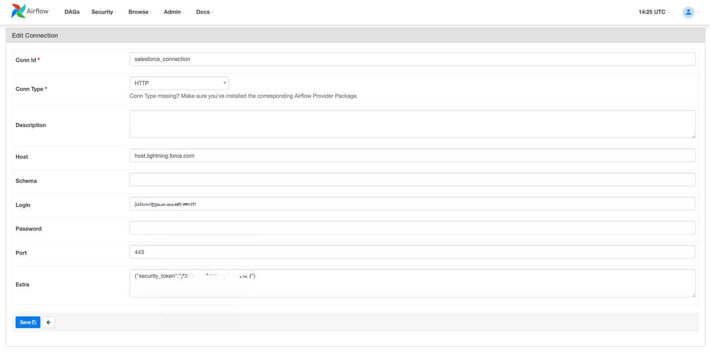
How Roche democratized access to data with Google Sheets and Amazon Redshift Data API

Post Syndicated from Dr. Yannick Misteli original https://aws.amazon.com/blogs/big-data/how-roche-democratized-access-to-data-with-google-sheets-and-amazon-redshift-data-api/

This post was co-written with Dr. Yannick Misteli, João Antunes, and Krzysztof Wisniewski from the Roche global Platform and ML engineering team as the lead authors.

Roche is a Swiss multinational healthcare company that operates worldwide. Roche is the largest pharmaceutical company in the world and the leading provider of cancer treatments globally.

In this post, Roche’s global Platform and machine learning (ML) engineering team discuss how they used Amazon Redshift data API to democratize access to the data in their Amazon Redshift data warehouse with Google Sheets (gSheets).

Business needs

Go-To-Market (GTM) is the domain that lets Roche understand customers and create and deliver valuable services that meet their needs. This lets them get a better understanding of the health ecosystem and provide better services for patients, doctors, and hospitals. It extends beyond health care professionals (HCPs) to a larger Healthcare ecosystem consisting of patients, communities, health authorities, payers, providers, academia, competitors, etc. Data and analytics are essential to supporting our internal and external stakeholders in their decision-making processes through actionable insights.

For this mission, Roche embraced the modern data stack and built a scalable solution in the cloud.

Driving true data democratization requires not only providing business leaders with polished dashboards or data scientists with SQL access, but also addressing the requirements of business users that need the data. For this purpose, most business users (such as Analysts) leverage Excel—or gSheet in the case of Roche—for data analysis.

Providing access to data in Amazon Redshift to these gSheets users is a non-trivial problem. Without a powerful and flexible tool that lets data consumers use self-service analytics, most organizations will not realize the promise of the modern data stack. To solve this problem, we want to empower every data analyst who doesn’t have an SQL skillset with a means by which they can easily access and manipulate data in the applications that they are most familiar with.

The Roche GTM organization uses the Redshift Data API to simplify the integration between gSheets and Amazon Redshift, and thus facilitate the data needs of their business users for analytical processing and querying. The Amazon Redshift Data API lets you painlessly access data from Amazon Redshift with all types of traditional, cloud-native, and containerized, serverless web service-based applications and event-driven applications. Data API simplifies data access, ingest, and egress from languages supported with AWS SDK, such as Python, Go, Java, Node.js, PHP, Ruby, and C++ so that you can focus on building applications as opposed to managing infrastructure. The process they developed using Amazon Redshift Data API has significantly lowered the barrier for entry for new users without needing any data warehousing experience.

Use-Case

In this post, you will learn how to integrate Amazon Redshift with gSheets to pull data sets directly back into gSheets. These mechanisms are facilitated through the use of the Amazon Redshift Data API and Google Apps Script. Google Apps Script is a programmatic way of manipulating and extending gSheets and the data that they contain.

Architecture

It is possible to include publicly available JS libraries such as JQuery-builder provided that Apps Script is natively a cloud-based Javascript platform.

The JQuery builder library facilitates the creation of standard SQL queries via a simple-to-use graphical user interface. The Redshift Data API can be used to retrieve the data directly to gSheets with a query in place. The following diagram illustrates the overall process from a technical standpoint:

Even though AppsScript is, in fact, Javascript, the AWS-provided SDKs for the browser (NodeJS and React) cannot be used on the Google platform, as they require specific properties that are native to the underlying infrastructure. It is possible to authenticate and access AWS resources through the available API calls. Here is an example of how to achieve that.

You can use an access key ID and a secret access key to authenticate the requests to AWS by using the code in the link example above. We recommend following the least privilege principle when granting access to this programmatic user, or assuming a role with temporary credentials. Since each user will require a different set of permissions on the Redshift objects—database, schema, and table—each user will have their own user access credentials. These credentials are safely stored under the AWS Secrets Manager service. Therefore, the programmatic user needs a set of permissions that enable them to retrieve secrets from the AWS Secrets Manager and execute queries against the Redshift Data API.

Code example for AppScript to use Data API

In this section, you will learn how to pull existing data back into a new gSheets Document. This section will not cover how to parse the data from the JQuery-builder library, as it is not within the main scope of the article.

<script src="https://cdn.jsdelivr.net/npm/jQuery-QueryBuilder/dist/js/query-builder.standalone.min.js"></script>    
  1. In the AWS console, go to Secrets Manager and create a new secret to store the database credentials to access the Redshift Cluster: username and password. These will be used to grant Redshift access to the gSheets user.
  2. In the AWS console, create a new IAM user with programmatic access, and generate the corresponding Access Key credentials. The only set of policies required for this user is to be able to read the secret created in the previous step from the AWS Secrets Manager service and to query the Redshift Data API.

    Below is the policy document:

    {
      "Version": "2012-10-17",
      "Statement": [
        {
          "Sid": "VisualEditor0",
          "Effect": "Allow",
          "Action": [
            "secretsmanager:GetSecretValue",
            "secretsmanager:DescribeSecret"
          ],
          "Resource": "arn:aws:secretsmanager:*::secret:*"
        },
        {
          "Sid": "VisualEditor1",
          "Effect": "Allow",
          "Action": "secretsmanager:ListSecrets",
          "Resource": "*"
        },
        {
          "Sid": "VisualEditor2",
          "Effect": "Allow",
          "Action": "redshift-data:*",
          "Resource": "arn:aws:redshift:*::cluster:*"
        }
      ]
    }

  3. Access the Google Apps Script console. Create an aws.gs file with the code available here. This will let you perform authenticated requests to the AWS services by providing an access key and a secret access key.
  4. Initiate the AWS variable providing the access key and secret access key created in step 3.
    AWS.init("<ACCESS_KEY>", "<SECRET_KEY>");

  5. Request the Redshift username and password from the AWS Secrets Manager:
    function runGetSecretValue_(secretId) {
     
      var resultJson = AWS.request(
        	getSecretsManagerTypeAWS_(),
        	getLocationAWS_(),
        	'secretsmanager.GetSecretValue',
        	{"Version": getVersionAWS_()},
        	method='POST',
        	payload={          
          	"SecretId" : secretId
        	},
        	headers={
          	"X-Amz-Target": "secretsmanager.GetSecretValue",
          	"Content-Type": "application/x-amz-json-1.1"
        	}
      );
     
      Logger.log("Execute Statement result: " + resultJson);
      return JSON.parse(resultJson);
     
    }

  6. Query a table using the Amazon Redshift Data API:
    function runExecuteStatement_(sql) {
     
      var resultJson = AWS.request(
        	getTypeAWS_(),
        	getLocationAWS_(),
        	'RedshiftData.ExecuteStatement',
        	{"Version": getVersionAWS_()},
        	method='POST',
        	payload={
          	"ClusterIdentifier": getClusterIdentifierReshift_(),
          	"Database": getDataBaseRedshift_(),
          	"DbUser": getDbUserRedshift_(),
          	"Sql": sql
        	},
        	headers={
          	"X-Amz-Target": "RedshiftData.ExecuteStatement",
          	"Content-Type": "application/x-amz-json-1.1"
        	}
      ); 
     
      Logger.log("Execute Statement result: " + resultJson); 

  7. The result can then be displayed as a table in gSheets:
    function fillGsheet_(recordArray) { 
     
      adjustRowsCount_(recordArray);
     
      var rowIndex = 1;
      for (var i = 0; i < recordArray.length; i++) {  
           
    	var rows = recordArray[i];
    	for (var j = 0; j < rows.length; j++) {
      	var columns = rows[j];
      	rowIndex++;
      	var columnIndex = 'A';
         
      	for (var k = 0; k < columns.length; k++) {
           
        	var field = columns[k];       
        	var value = getFieldValue_(field);
        	var range = columnIndex + rowIndex;
        	addToCell_(range, value);
     
        	columnIndex = nextChar_(columnIndex);
     
      	}
     
    	}
     
      }
     
    }

  8. Once finished, the Apps Script can be deployed as an Addon that enables end-users from an entire organization to leverage the capabilities of retrieving data from Amazon Redshift directly into their spreadsheets. Details on how Apps Script code can be deployed as an Addon can be found here.

How users access Google Sheets

  1. Open a gSheet, and go to manage addons -> Install addon:
  2. Once the Addon is successfully installed, select the Addon menu and select Redshift Synchronization. A dialog will appear prompting the user to select the combination of database, schema, and table from which to load the data.
  3. After choosing the intended table, a new panel will appear on the right side of the screen. Then, the user is prompted to select which columns to retrieve from the table, apply any filtering operation, and/or apply any aggregations to the data.
  4. Upon submitting the query, app scripts will translate the user selection into a query that is sent to the Amazon Redshift Data API. Then, the returned data is transformed and displayed as a regular gSheet table:

Security and Access Management

In the scripts above, there is a direct integration between AWS Secrets Manager and Google Apps Script. The scripts above can extract the currently-authenticated user’s Google email address. Using this value and a set of annotated tags, the script can appropriately pull the user’s credentials securely to authenticate the requests made to the Amazon Redshift cluster. Follow these steps to set up a new user in an existing Amazon Redshift cluster. Once the user has been created, follow these steps for creating a new AWS Secrets Manager secret for your cluster. Make sure that the appropriate tag is applied with the key of “email” along with the corresponding user’s Google email address. Here is a sample configuration that is used for creating Redshift groups, users, and data shares via the Redshift Data API:

connection:
 redshift_super_user_database: dev
 redshift_secret_name: dev_
 redshift_cluster_identifier: dev-cluster
 redshift_secrets_stack_name: dev-cluster-secrets
 environment: dev
 aws_region: eu-west-1
 tags:
   - key: "Environment"
 	value: "dev"
users:
 - name: user1
   email: [email protected]
 data_shares:
 - name: test_data_share
   schemas:
 	- schema1
   redshift_namespaces:
 	- USDFJIL234234WE
group:
 - name: readonly
   users:
 	- user1
   databases:
 	- database: database1
   	exclude-schemas:
     	- public
     	- pg_toast
     	- catalog_history
   	include-schemas:
     	- schema1
   	grant:
     	- select

Operational Metrics and Improvement

Providing access to live data that is hosted in Redshift directly to the business users and enabling true self-service decrease the burden on platform teams to provide data extracts or other mechanisms to deliver up-to-date information. Additionally, by not having different files and versions of data circulating, the business risk of reporting different key figures or KPI can be reduced, and an overall process efficiency can be achieved.

The initial success of this add-on in GTM led to the extension of this to a broader audience, where we are hoping to serve hundreds of users with all of the internal and public data in the future.

Conclusion

In this post, you learned how to create new Amazon Redshift tables and pull existing Redshift tables into a Google Sheet for business users to easily integrate with and manipulate data. This integration was seamless and demonstrated how easy the Amazon Redshift Data API makes integration with external applications, such as Google Sheets with Amazon Redshift. The outlined use-cases above are just a few examples of how the Amazon Redshift Data API can be applied and used to simplify interactions between users and Amazon Redshift clusters.


About the Authors

Dr. Yannick Misteli is leading cloud platform and ML engineering teams in global product strategy (GPS) at Roche. He is passionate about infrastructure and operationalizing data-driven solutions, and he has broad experience in driving business value creation through data analytics.

João Antunes is a Data Engineer in the Global Product Strategy (GPS) team at Roche. He has a track record of deploying Big Data batch and streaming solutions for the telco, finance, and pharma industries.

Krzysztof Wisniewski is a back-end JavaScript developer in the Global Product Strategy (GPS) team at Roche. He is passionate about full-stack development from the front-end through the back-end to databases.

Matt Noyce is a Senior Cloud Application Architect at AWS. He works together primarily with Life Sciences and Healthcare customers to architect and build solutions on AWS for their business needs.

Debu Panda, a Principal Product Manager at AWS, is an industry leader in analytics, application platform, and database technologies, and has more than 25 years of experience in the IT world. Debu has published numerous articles on analytics, enterprise Java, and databases and has presented at multiple conferences such as re:Invent, Oracle Open World, and Java One. He is lead author of the EJB 3 in Action (Manning Publications 2007, 2014) and Middleware Management (Packt).

TrueBlue uses Amazon QuickSight to deliver more accurate pricing and grow business

Post Syndicated from Robert Ward original https://aws.amazon.com/blogs/big-data/trueblue-uses-amazon-quicksight-to-deliver-more-accurate-pricing-and-grow-business/

This is a guest post by TrueBlue. In their own words, “Founded in 1989, TrueBlue provides specialized workforce solutions, including staffing, talent management, and recruitment process outsourcing (RPO). In 2020, the company connected approximately 490,000 people with work.”

At TrueBlue, we offer solutions that help employers connect with workers worldwide. Every day, sales teams at our 500-plus locations offer our customers job quotes. These quotes show our staff the hourly rates they should charge and what the gross margin might be on a bill rate.

As part of our work, our sales professionals use a concept called lockout, which is the process for approving sales orders below standard margins. As our company has grown, these approval requests have skyrocketed. We have more than 850 people bidding for potential customers at any time, but only a few dozen managers can approve lockout requests. The number of requests that managers had in their inboxes was increasingly overwhelming and took time away from more important daily tasks. They wanted a way to avoid the process altogether by standardizing job rate information.

In this post, I discuss the steps we took to solve our problem using data analysis and Amazon QuickSight.

Identifying regional pricing differences

To begin, I looked at hourly worker rates across all our locations and added state tax data and other information. That gave me our customer billing rate, plus the overhead to calculate the gross margin. Through my research, I discovered that regionality is important in determining different rates and margins, and that pricing isn’t consistent overall.

Our sales leaders wanted to take this to the next level and figure out the gross margin they would need to maintain a specific hourly billing rate. I could only see 7 months of information, but it amounted to nearly 1 million rows of data. We needed a fast, easy way to use spreadsheet software to find what we were looking for.

Using QuickSight to give sales teams better pricing data

In 2020, we decided to go all in on AWS to create a new data lake and invest in other business intelligence (BI) solutions. After speaking with the AWS team, we learned that QuickSight, a powerful BI service that runs on AWS, could give us the detailed filtering and analytical capabilities we needed.

We used QuickSight to create a new customer job quoting engine for our sales teams in 40 of our branch offices. This solution provides our team with the price quotes that optimize profit margins and the data to calculate the precise charge in each market, all of which can be quickly accessed on their laptops. Now, the lockout requests are disappearing because the sales teams have the information at their fingertips and don’t need to ask for approvals. And because our sales leaders don’t have to read through countless emails every day, they can focus on more value-added tasks.

The following diagram illustrates our solution workflow, which sends data from AWS Database Migration Service (AWS DMS) through a data pipeline to Amazon Athena for analysis, and ultimately to QuickSight.

Boosting customer retention and acquisition by 3%

With the data we’re getting from QuickSight, we can present our customers with more accurate pricing and billing information. As a result, we’ve increased new customer acquisition and retention. Our sales teams are closing phone deals at rates 3% higher than an internal sales control group. We’ve also seen an 11% increase in gross margin for the market in which we’ve used the job quoting engine the longest. Applying the data we have now is really making a difference in our business.

And with the live data powering QuickSight, we’re able to increase our margins. Every time we pay someone, our pricing is updated based on real-time regional data. The solution is always adapting to market conditions, so we can give customers nationwide a price with detailed market segmentation. For example, they can see why we’re charging more in the Midwest than in the South.

Being more transparent with customers

Our frontline sales teams can be more transparent about pricing with potential customers because they have better, more accurate pricing data. When a salesperson is on the phone with a customer, they can view the data in QuickSight and accurately explain what’s going on in a specific market. The pricing information is no longer an estimate; it’s completely accurate and up to date, and we can talk more confidently about what’s driving the cost, such as local conditions or risk ratings.

Another advantage of QuickSight and AWS is the agility and speed they give us. With AWS services, we can control how quickly to roll out the solution and who gets access. And we have more flexibility with AWS, so we can change things as we go and create better, faster tools for our internal teams without relying on a time-consuming, cumbersome development process. We can try things tomorrow that would have previously taken us 6 weeks to get into production, giving salespeople the new features they ask for quickly. And as a rapid prototyping vehicle, QuickSight is perfect for defining the next generation of job quoting packages that we’ll create for our customers.

Our job quoting tool isn’t just helping our frontline sales employees, it’s also benefiting staffing specialists, branch managers, market managers, and even regional and senior vice presidents. They can all see pricing averages and trends (as in the following screenshot), and select the data for specific markets or TrueBlue branches.

Conclusion

The downstream implications of our new job quoting tool powered by QuickSight are huge. Now conversations are happening at the right level, with the right kinds of customers driving more value for our business.


About the Authors

Robert Ward is the Senior Director of Technology at PeopleReady. His teams are responsible for delivering data science and machine learning solutions, strategy and data insights, democratized data, and business analytics solutions. PeopleReady is modernizing how the North American staffing industry connects people with work. Robert Ward is driven to craft innovations for desired outcomes.

Ryan Coyle is the AWS Account Manager for TrueBlue. He has partnered with TrueBlue on their digital transformation efforts since the beginning of 2020. In this function he has collaborated with them to close on-premises datacenter facilities, develop and deliver new products to market, and deliver data driven results to TrueBlue business units.

Shivani Sharma is one of the Account Managers supporting TrueBlue. She joined the team July 2020 where she partners with TrueBlue to drive and collaborate on their transformation initiatives.

Integral Ad Science secures self-service data lake using AWS Lake Formation

Post Syndicated from Mat Sharpe original https://aws.amazon.com/blogs/big-data/integral-ad-science-secures-self-service-data-lake-using-aws-lake-formation/

This post is co-written with Mat Sharpe, Technical Lead, AWS & Systems Engineering from Integral Ad Science.

Integral Ad Science (IAS) is a global leader in digital media quality. The company’s mission is to be the global benchmark for trust and transparency in digital media quality for the world’s leading brands, publishers, and platforms. IAS does this through data-driven technologies with actionable real-time signals and insight.

In this post, we discuss how IAS uses AWS Lake Formation and Amazon Athena to efficiently manage governance and security of data.

The challenge

IAS processes over 100 billion web transactions per day. With strong growth and changing seasonality, IAS needed a solution to reduce cost, eliminate idle capacity during low utilization periods, and maximize data processing speeds during peaks to ensure timely insights for customers.

In 2020, IAS deployed a data lake in AWS, storing data in Amazon Simple Storage Service (Amazon S3), cataloging its metadata in the AWS Glue Data Catalog, ingesting and processing using Amazon EMR, and using Athena to query and analyze the data. IAS wanted to create a unified data platform to meet its business requirements. Additionally, IAS wanted to enable self-service analytics for customers and users across multiple business units, while maintaining critical controls over data privacy and compliance with regulations such as GDPR and CCPA. To accomplish this, IAS needed to securely ingest and organize real-time and batch datasets, as well as secure and govern sensitive customer data.

To meet the dynamic nature of IAS’s data and use cases, the team needed a solution that could define access controls by attribute, such as classification of data and job function. IAS processes significant volumes of data and this continues to grow. To support the volume of data, IAS needed the governance solution to scale in order to create and secure many new daily datasets. This meant IAS could enable self-service access to data from different tools, such as development notebooks, the AWS Management Console, and business intelligence and query tools.

To address these needs, IAS evaluated several approaches, including a manual ticket-based onboarding process to define permissions on new datasets, many different AWS Identity and Access Management (IAM) policies, and an AWS Lambda based approach to automate defining Lake Formation table and column permissions triggered by changes in security requirements and the arrival of new datasets.

Although these approaches worked, they were complex and didn’t support the self-service experience that IAS data analysts required.

Solution overview

IAS selected Lake Formation, Athena, and Okta to solve this challenge. The following architectural diagram shows how the company chose to secure its data lake.

The solution needed to support data producers and consumers in multiple AWS accounts. For brevity, this diagram shows a central data lake producer that includes a set of S3 buckets for raw and processed data. Amazon EMR is used to ingest and process the data, and all metadata is cataloged in the data catalog. The data lake consumer account uses Lake Formation to define fine-grained permissions on datasets shared by the producer account; users logging in through Okta can run queries using Athena and be authorized by Lake Formation.

Lake Formation enables column-level control, and all Amazon S3 access is provisioned via a Lake Formation data access role in the query account, ensuring only that service can access the data. Each business unit with access to the data lake is provisioned with an IAM role that only allows limited access to:

  • That business unit’s Athena workgroup
  • That workgroup’s query output bucket
  • The lakeformation:GetDataAccess API

Because Lake Formation manages all the data access and permissions, the configuration of the user’s role policy in IAM becomes very straightforward. By defining an Athena workgroup per business unit, IAS also takes advantage of assigning per-department billing tags and query limits to help with cost management.

Define a tag strategy

IAS commonly deals with two types of data: data generated by the company and data from third parties. The latter usually includes contractual stipulations on privacy and use.

Some data sets require even tighter controls, and defining a tag strategy is one key way that IAS ensures compliance with data privacy standards. With the tag-based access controls in Lake Formation IAS can define a set of tags within an ontology that is assigned to tables and columns. This ensures users understand available data and whether or not they have access. It also helps IAS manage privacy permissions across numerous tables with new ones added every day.

At a simplistic level, we can define policy tags for class with private and non-private, and for owner with internal and partner.

As we progressed, our tagging ontology evolved to include individual data owners and data sources within our product portfolio.

Apply tags to data assets

After IAS defined the tag ontology, the team applied tags at the database, table, and column level to manage permissions. Tags are inherited, so they only need to be applied at the highest level. For example, IAS applied the owner and class tags at the database level and relied on inheritance to propagate the tags to all the underlying tables and columns. The following diagram shows how IAS activated a tagging strategy to distinguish between internal and partner datasets , while classifying sensitive information within these datasets.

Only a small number of columns contain sensitive information; IAS relied on inheritance to apply a non-private tag to the majority of the database objects and then overrode it with a private tag on a per-column basis.

The following screenshot shows the tags applied to a database on the Lake Formation console.

With its global scale, IAS needed a way to automate how tags are applied to datasets. The team experimented with various options including string matching on column names, but the results were unpredictable in situations where unexpected column names are used (ipaddress vs. ip_address, for example). Ultimately, IAS incorporated metadata tagging into its existing infrastructure as code (IaC) process, which gets applied as part of infrastructure updates.

Define fine-grained permissions

The final piece of the puzzle was to define permission rules to associate with tagged resources. The initial data lake deployment involved creating permission rules for every database and table, with column exclusions as necessary. Although these were generated programmatically, it added significant complexity when the team needed to troubleshoot access issues. With Lake Formation tag-based access controls, IAS reduced hundreds of permission rules down to precisely two rules, as shown in the following screenshot.

When using multiple tags, the expressions are logically ANDed together. The preceding statements permit access only to data tagged non-private and owned by internal.

Tags allowed IAS to simplify permission rules, making it easy to understand, troubleshoot, and audit access. The ability to easily audit which datasets include sensitive information and who within the organization has access to them made it easy to comply with data privacy regulations.

Benefits

This solution provides self-service analytics to IAS data engineers, analysts, and data scientists. Internal users can query the data lake with their choice of tools, such as Athena, while maintaining strong governance and auditing. The new approach using Lake Formation tag-based access controls reduces the integration code and manual controls required. The solution provides the following additional benefits:

  • Meets security requirements by providing column-level controls for data
  • Significantly reduces permission complexity
  • Reduces time to audit data security and troubleshoot permissions
  • Deploys data classification using existing IaC processes
  • Reduces the time it takes to onboard data users including engineers, analysts, and scientists

Conclusion

When IAS started this journey, the company was looking for a fully managed solution that would enable self-service analytics while meeting stringent data access policies. Lake Formation provided IAS with the capabilities needed to deliver on this promise for its employees. With tag-based access controls, IAS optimized the solution by reducing the number of permission rules from hundreds down to a few, making it even easier to manage and audit. IAS continues to analyze data using more tools governed by Lake Formation.


About the Authors

Mat Sharpe is the Technical Lead, AWS & Systems Engineering at IAS where he is responsible for the company’s AWS infrastructure and guiding the technical teams in their cloud journey. He is based in New York.

Brian Maguire is a Solution Architect at Amazon Web Services, where he is focused on helping customers build their ideas in the cloud. He is a technologist, writer, teacher, and student who loves learning. Brian is the co-author of the book Scalable Data Streaming with Amazon Kinesis.

Danny Gagne is a Solutions Architect at Amazon Web Services. He has extensive experience in the design and implementation of large-scale high-performance analysis systems, and is the co-author of the book Scalable Data Streaming with Amazon Kinesis. He lives in New York City.

How Rapid7 built multi-tenant analytics with Amazon Redshift using near-real-time datasets

Post Syndicated from Rahul Monga original https://aws.amazon.com/blogs/big-data/how-rapid7-built-multi-tenant-analytics-with-amazon-redshift-using-near-real-time-datasets/

This is a guest post co-written by Rahul Monga, Principal Software Engineer at Rapid7.

Rapid7 InsightVM is a vulnerability assessment and management product that provides visibility into the risks present across an organization. It equips you with the reporting, automation, and integrations needed to prioritize and fix those vulnerabilities in a fast and efficient manner. InsightVM has more than 5,000 customers across the globe, runs exclusively on AWS, and is available for purchase on AWS Marketplace.

To provide near-real-time insights to InsightVM customers, Rapid7 has recently undertaken a project to enhance the dashboards in their multi-tenant software as a service (SaaS) portal with metrics, trends, and aggregated statistics on vulnerability information identified in their customer assets. They chose Amazon Redshift as the data warehouse to power these dashboards due to its ability to deliver fast query performance on gigabytes to petabytes of data.

In this post, we discuss the design options that Rapid7 evaluated to build a multi-tenant data warehouse and analytics platform for InsightVM. We will deep dive into the challenges and solutions related to ingesting near-real-time datasets and how to create a scalable reporting solution that can efficiently run queries across more than 3 trillion rows. This post also discusses an option to address the scenario where a particular customer outgrows the average data access needs.

This post uses the terms customers, tenants, and organizations interchangeably to represent Rapid7 InsightVM customers.

Background

To collect data for InsightVM, customers can use scan engines or Rapid7’s Insight Agent. Scan engines allow you to collect vulnerability data on every asset connected to a network. This data is only collected when a scan is run. Alternatively, you can install the Insight Agent on individual assets to collect and send asset change information to InsightVM numerous times each day. The agent also ensures that asset data is sent to InsightVM regardless of whether or not the asset is connected to your network.

Data from scans and agents is sent in the form of packed documents, in micro-batches of hundreds of events. Around 500 documents per second are received across customers, and each document is around 2 MB in size. On a typical day, InsightVM processes 2–3 trillion rows of vulnerability data, which translates to around 56 GB of compressed data for a large customer. This data is normalized and processed by InsightVM’s vulnerability management engine and streamed to the data warehouse system for near-real-time availability of data for analytical insights to customers.

Architecture overview

In this section, we discuss the overall architectural setup for the InsightVM system.

Scan engines and agents collect and send asset information to the InsightVM cloud. Asset data is pooled, normalized, and processed to identify vulnerabilities. This is stored in an Amazon ElastiCache for Redis cluster and also pushed to Amazon Kinesis Data Firehouse for use in near-real time by InsightVM’s analytics dashboards. Kinesis Data Firehose delivers raw asset data to an Amazon Simple Storage Service (Amazon S3) bucket. The data is transformed using a custom developed ingestor service and stored in a new S3 bucket. The transformed data is then loaded into the Redshift data warehouse. Amazon Simple Notification Service (Amazon SNS), Amazon Simple Queue Service (Amazon SQS), and AWS Lambda are used to orchestrate this data flow.  In addition, to identify the latest timestamp of vulnerability data for assets, an auxiliary table is maintained and updated periodically with the update logic in the Lambda function, which is triggered through an Amazon CloudWatch event rule. Custom-built middleware components interface between the web user interface (UI) and the Amazon Redshift cluster to fetch asset information for display in dashboards.

The following diagram shows the implementation architecture of InsightVM, including the data warehouse system:

Rapid-7 Multi-tenant Architecture

The architecture has built-in tenant isolation because data access is abstracted through the API. The application uses a dimensional model to support low-latency queries and extensibility for future enhancements.

Amazon Redshift data warehouse design: Options evaluated and selection

Considering Rapid7’s need for near-real-time analytics at any scale, the InsightVM data warehouse system is designed to meet the following requirements:

  • Ability to view asset vulnerability data at near-real time, within 5–10 minutes of ingest
  • Less than 5 seconds’ latency when measured at 95 percentiles (p95) for reporting queries
  • Ability to support 15 concurrent queries per second, with the option to support more in the future
  • Simple and easy-to-manage data warehouse infrastructure
  • Data isolation for each customer or tenant

Rapid7 evaluated Amazon Redshift RA3 instances to support these requirements. When designing the Amazon Redshift schema to support these goals, they evaluated the following strategies:

  • Bridge model – Storage and access to data for each tenant is controlled at the individual schema level in the same database. In this approach, multiple schemas are set up, where each schema is associated with a tenant, with the same exact structure of the dimensional model.
  • Pool model – Data is stored in a single database schema for all tenants, and a new column (tenant_id) is used to scope and control access to individual tenant data. Access to the multi-tenant data is controlled using API-level access to the tables. Tenants aren’t aware of the underlying implementation of the analytical system and can’t query them directly.

For more information about multi-tenant models, see Implementing multi-tenant patterns in Amazon Redshift using data sharing.

Initially when evaluating the bridge model, it provided an advantage for tenant-only data for queries, plus the ability to decouple a tenant to an independent cluster if they outgrow the resources that are available in the single cluster. Also, when the p95 metrics were evaluated in this setup, the query response times were less than 5 seconds, because each tenant data is isolated into smaller tables. However, the major concern with this approach was with the near-real-time data ingestion into over 50,000 tables (5,000 customer schemas x approximately 10 tables per schema) every 5 minutes. Having thousands of commits every minute into an online analytical processing (OLAP) system like Amazon Redshift can lead to most resources being exhausted in the ingestion process. As a result, the application suffers query latencies as data grows.

The pool model provides a simpler setup, but the concern was with query latencies when multiple tenants access the application from the same tables. Rapid7 hoped that these concerns would be addressed by using Amazon Redshift’s support for massively parallel processing (MPP) to enable fast execution of most complex queries operating on large amounts of data. With the right table design using the right sort and distribution keys, it’s possible to optimize the setup. Furthermore, with automatic table optimization, the Amazon Redshift cluster can automatically make these determinations without any manual input.

Rapid7 evaluated both the pool and bridge model designs, and decided to implement the pool model. This model provides simplified data ingestion and can support query latencies of under 5 seconds at p95 with the right table design. The following table summarizes the results of p95 tests conducted with the pool model setup.

Query P95
Large customer: Query with multiple joins, which list assets, their vulnerabilities, and all their related attributes, with aggregated metrics for each asset, and filters to scope assets by attributes like location, names, and addresses Less than 4 seconds
Large customer: Query to return vulnerability content information given a list of vulnerability identifiers Less than 4 seconds

Tenet isolation and security

Tenant isolation is fundamental to the design and development of SaaS systems. It enables SaaS providers to reassure customers that, even in a multi-tenant environment, their resources can’t be accessed by other tenants.

With the Amazon Redshift table design using the pool model, Rapid7 built a separate data access layer in the middleware that templatized queries, augmented with runtime parameter substitution to uniquely filter specific tenant and organization data.

The following is a sample of templatized query:

<#if useDefaultVersion()>
currentAssetInstances AS (
SELECT tablename.*
FROM tablename
<#if (applyTags())>
JOIN dim_asset_tag USING (organization_id, attribute2, attribute3)
</#if>
WHERE organization_id ${getOrgIdFilter()}
<#if (applyTags())>
AND tag_id IN ($(tagIds))
</#if>
),
</#if>

The following is a Java interface snippet to populate the template:

public interface TemplateParameters {

boolean useDefaultVersion(); boolean useVersion(); default Set<String> getVersions() {
return null;
} default String getVersionJoin(String var1) {
return "";
}

String getTemplateName();

String getOrgIdString();

default String getOrgIdFilter() {
return "";
}

Every query uses organization_id and additional parameters to uniquely access tenant data. During runtime, organization_id and other metadata are extracted from the secured JWT token that is passed to middleware components after the user is authenticated in the Rapid7 cloud platform.

Best practices and lessons learned

To fully realize the benefits of the Amazon Redshift architecture and design for the multiple tenants & near real-time ingestion, considerations on the table design allow you to take full advantage of the massively parallel processing and columnar data storage. In this section, we discuss the best practices and lessons learned from building this solution.

Sort key for effective data pruning

Sorting a table on an appropriate sort key can accelerate query performance, especially queries with range-restricted predicates, by requiring fewer table blocks to be read from disk. To have Amazon Redshift choose the appropriate sort order, the AUTO option was utilized. Automatic table optimization continuously observes how queries interact with tables and discovers the right sort key for the table. To effectively prune the data by the tenant, organization_id is identified as the sort key to perform the restricted scans. Furthermore, because all queries are routed through the data access layer, organization_id is automatically added in the predicate conditions to ensure effective use of the sort keys.

Micro-batches for data ingestion

Amazon Redshift is designed for large data ingestion, rather than transaction processing. The cost of commits is relatively high, and excessive use of commits can result in queries waiting for access to the commit queue. Data is micro-batched during ingestion as it arrives for multiple organizations. This results in fewer transactions and commits when ingesting the data.

Load data in bulk

If you use multiple concurrent COPY commands to load one table from multiple files, Amazon Redshift is forced to perform a serialized load, and this type of load is much slower.

The Amazon Redshift manifest file is used to ingest the datasets that span multiple files in a single COPY command, which allows fast ingestion of data in each micro-batch.

RA3 instances for data sharing

Rapid 7 uses Amazon Redshift RA3 instances, which enable data sharing to allow you to securely and easily share live data across Amazon Redshift clusters for reads. In this multi-tenant architecture when a tenant outgrows the average data access needs, it can be isolated to a separate cluster easily and independently scaled using the data sharing. This is accomplished by monitoring the STL_SCAN table to identify different tenants and isolate them to allow for independent scalability as needed.

Concurrency scaling for consistently fast query performance

When concurrency scaling is enabled, Amazon Redshift automatically adds additional cluster capacity when you need it to process an increase in concurrent read queries. To meet the uptick in user requests, the concurrency scaling feature is enabled to dynamically bring up additional capacity to provide consistent p95 values that meet Rapid7’s defined requirements for the InsightVM application.

Results and benefits

Rapid7 saw the following results from this architecture:

  • The new architecture has reduced the time required to make data accessible to customers to less than 5 minutes on average. The previous architecture had higher level of processing time variance, and could sometimes exceed 45 minutes
  • Dashboards load faster and have enhanced drill-down functionality, improving the end-user experience
  • With all data in a single warehouse, InsightVM has a single source of truth, compared to the previous solution where InsightVM had copies of data maintained in different databases and domains, which could occasionally get out of sync
  • The new architecture lowers InsightVM’s reporting infrastructure cost by almost three times, as compared to the previous architecture

Conclusion

With Amazon Redshift, the Rapid7 team has been able to centralize asset and vulnerability information for InsightVM customers. The team has simultaneously met its performance and management objectives with the use of a multi-tenant pool model and optimized table design. In addition, data ingestion via Kinesis Data Firehose and custom-built microservices to load data into Amazon Redshift in near-real time enabled Rapid7 to deliver asset vulnerability information to customers more than nine times faster than before, improving the InsightVM customer experience.


About the Authors

Rahul Monga is a Principal Software Engineer at Rapid7, currently working on the next iteration of InsightVM. Rahul’s focus areas are highly distributed cloud architectures and big data processing. Originally from the Washington DC area, Rahul now resides in Austin, TX with his wife, daughter, and adopted pup.

Sujatha Kuppuraju is a Senior Solutions Architect at Amazon Web Services (AWS). She works with ISV customers to help design secured, scalable and well-architected solutions on the AWS Cloud. She is passionate about solving complex business problems with the ever-growing capabilities of technology.

Thiyagarajan Arumugam is a Principal Solutions Architect at Amazon Web Services and designs customer architectures to process data at scale. Prior to AWS, he built data warehouse solutions at Amazon.com. In his free time, he enjoys all outdoor sports and practices the Indian classical drum mridangam.

How Tophatter improved stability and lowered costs by migrating to Amazon Redshift RA3

Post Syndicated from Julien DeFrance original https://aws.amazon.com/blogs/big-data/how-tophatter-improved-stability-and-lowered-costs-by-migrating-to-amazon-redshift-ra3/

This is a guest post co-written by Julien DeFrance of Tophatter and Jordan Myers of Etleap. Tophatter is a mobile discovery marketplace that hosts live auctions for products spanning every major category. Etleap, an AWS Advanced Tier Data & Analytics partner, is an extract, transform, load, and transform (ETLT) service built for AWS.

As a company grows, it continually seeks out solutions that help its teams achieve better performance and scale of their data analytics, especially when business growth has eclipsed current capabilities. Migrating to a new architecture is often a key component of this. However, a migration path that is painless, flexible, and supported is not always available.

In this post, we walk through how Tophatter—a virtual auction house where buyers and sellers interact, chat, and transact in diverse categories—recently migrated from DS2 to RA3 nodes in Amazon Redshift. We highlight the steps they took, how they improved stability and lowered costs, and the lessons other companies can follow.

Tophatter’s data storage and ETL architecture

Tophatter stores the majority of their product data in MySQL databases, while sending some webhook and web events to Amazon Simple Storage Service (Amazon S3). Additionally, some of their vendors drop data directly into dedicated S3 buckets. Etleap integrates with these sources. Every hour (according to the schedule configured by Tophatter), Etleap extracts all the new data that has been added or changed in the source, transforms the new data according to the pipeline rules defined by the user in the UI, and loads the resulting data into Amazon Redshift.

Tophatter relies on Mode Analytics and Looker for data analysis, and uses Etleap’s model feature based on Amazon Redshift materialized views to persist the results of frequently used business intelligence (BI) queries. Tophatter configures the update schedule of the model to happen at defined times or when certain source tables have been updated with new data.

Ultimately, these critical data pipelines fuel Tophatter dashboards that both internal analysts and users interact with.

The following diagram illustrates how Tophatter uses Etleap’s AWS-native extract, transform, and load (ETL) tool to ingest data from their operational databases, applications, and Amazon S3 into Amazon Redshift.

Company growth leads to data latency

Before the migration, Tophatter’s team operated 4 DS2 Reserved Instance (RI) nodes (ds2.xlarge) in Amazon Redshift, which use HDD drives as opposed to relatively faster SSDs.

As their user base expanded and online auction activity increased exponentially, Tophatter’s ETL needs grew. In response, Etleap seamlessly scaled to support their increased volume of ingestion pipelines and materialized data models. But Tophatter’s Amazon Redshift cluster—which they managed internally—wasn’t as easy to scale. When Amazon Redshift usage increased, Tophatter had to resize the cluster manually or reduce the frequency of certain analytics queries or models. Finding the optimal cluster size often required multiple iterations.

Due to the time-sensitive nature of data needed for live online auctions, Tophatter used automated monitoring to notify on-call engineers when data pipeline latency had exceeded the desired threshold. Latencies and errors began to pop up more frequently—at least once or twice a week. These events caused distress for the on-call engineers. When the issue couldn’t be resolved internally, they notified Etleap support, who typically recommended either canceling or reducing the frequency of certain long-running model queries.

While the issue was still being resolved, the latencies resulted in downstream issues for the analytics team, such as certain tables being out of sync with others, resulting in incorrect query results.

Migrating to Amazon Redshift RA3

To improve stability and reduce engineering maintenance, Tophatter decided to migrate from DS2 to RA3 nodes. Amazon Redshift RA3 with managed storage is the latest generation node type and would allow Tophatter to scale compute and storage independently.

With DS2 nodes, there was pressure to offload or archive historical data to other storage because of fixed storage limits. RA3 nodes with managed storage are an excellent fit for analytics workloads that require high storage capacity, such as operational analytics, where the subset of data that’s most important continually evolves over time.

Moving to the RA3 instance type would also enable Tophatter to capitalize on the latest features of Amazon Redshift, such as AQUA (Advanced Query Accelerator), Data Sharing, Amazon Redshift ML, and cross-VPC support.

RA3 migration upgrade program

Tophatter understood the benefits of migrating to RA3, but worried that their 3-year DS2 Reserved Instances commitment would present a roadblock. They still had 2 years remaining in their agreement and were unsure if an option was available that would allow them to change course.

They found out about the AWS RA3 upgrade program from the AWS account team, which helps customers convert their DS2 Reserved Instance commitments into RA3 without breaking the commitment agreement. This path enables you to seamlessly migrate from your legacy Amazon Redshift clusters to one of three RA3 node types: ra3.xlplus, ra3.4xlarge, or ra3.16xlarge.

Tophatter’s engagement with the program consisted of five steps:

  1. Engage with the AWS account team.
  2. Receive pricing information from the AWS account team.
  3. Schedule the migration.
  4. Purchase RA3 Reserved Instances.
  5. Submit a case to cancel their DS2 Reserved Instances.

Tophatter had the opportunity to evaluate three options for their RA3 migration:

  • Elastic resize – This is the most efficient way to change the instance type and update the nodes in your Amazon Redshift cluster. The cluster endpoint doesn’t change and the downtime during resize is minimal.
  • Snapshot and restore method – Choose the snapshot and restore method if elastic resize is unavailable (from a mismatch between slice and node count). Or, use this method to minimize the amount of time it takes to write to your production database.
  • Classic resize – Choose the classic resize method if it’s the only option available. For single-node DS2 clusters, only a classic resize can be performed to convert the cluster into a multi-node cluster.

Achieving operational goals

Tophatter worked closely with their AWS account team for the migration and chose elastic resize due to the minimal downtime that option presented as well as prior experience using it. They completed the migration in under 2 hours, which included the requisite pre- and post-testing. As a pre-migration step, they took a snapshot of the cluster and were prepared to restore it if something went wrong.

After migrating to a 2 node ra3.4xlarge cluster, the Tophatter team realized numerous benefits:

  • Storage with up to 256 TB of Amazon Redshift managed storage for their cluster
  • Dramatically reduced latency of ingestion and data modeling
  • Control of the compute and storage capacities and costs, independently
  • Better system stability, with latency incidents requiring on-call engineer responses dropping to near zero

The following graph illustrates the average latency of a typical ingestion pipeline before and after the migration from DS2 to RA3.

Conclusion

When Tophatter set out to migrate their DS2 instances to RA3, they were unaware of the AWS RA3 upgrade program and its benefits. They were happy to learn that the program avoided the administrative overhead of getting approvals ahead of time for various specific configurations, and let them try several options in order to find a stable configuration.

Tophatter migrated from DS2 to RA3 without breaking their current commitment and enhanced their analytics to be agile and versatile. Now, Tophatter is aiming to realize greater scaling benefits to support its exponential growth by exploring new RA3 features such as:

  • Amazon Redshift Data Sharing – Provides instant, granular, high-performance data access without data copies or movement
  • Amazon Redshift ML – Allows you to create, train, and apply machine learning models using SQL commands in Amazon Redshift
  • AQUA – Provides a new distributed and hardware accelerated cache that brings compute to the storage layer for Amazon Redshift and delivers up to 10 times faster query performance than other enterprise cloud data warehouses
  • Cross-VPC support for Amazon Redshift – With an Amazon Redshift-managed VPC endpoint, you can privately access your Amazon Redshift data warehouse within your VPC from your client applications in another VPC within the same AWS account, another AWS account, or running on-premises without using public IPs or requiring encrypted traffic to traverse the internet

We hope Tophatter’s migration journey can help other AWS customers reap the benefits from the AWS RA3 upgrade program from DS2 or DC2 cluster families to RA3. We believe this enables better performance and cost benefits while unlocking valuable new Amazon Redshift features.


About the Authors

Julien DeFrance is a Principal Software Engineer at Tophatter based out of San Francisco. With a strong focus on backend and cloud infrastructure, he is part of the Logistics Engineering Squad, building and supporting integrations with third parties such as sellers, ERP systems, and carriers, architecting and implementing solutions to help optimize cost efficiency and service quality. Julien holds two AWS Certifications (Cloud Practitioner, Solutions Architect – Associate).


Jordan Myers is an engineer at Etleap with 5 years of experience in programming ETL software. In addition to programming, he provides deep-level technical customer support and writes technical documentation


Jobin George is a Big Data Solutions Architect with more than a decade of experience designing and implementing large-scale big data and analytics solutions. He provides technical guidance, design advice, and thought leadership to some of the key AWS customers and big data partners.


Maneesh Sharma is a Senior Database Engineer with Amazon Redshift. He works and collaborates with various Amazon Redshift Partners to drive better integration. In his spare time, he likes running, playing ping pong, and exploring new travel destinations.

Zabbix 5.0 – My happiness and disenchantment

Post Syndicated from Dennis Ananiev original https://blog.zabbix.com/zabbix-5-0-my-happiness-and-disenchantment/14107/

Zabbix is an open-source solution, and all features are available out of the box for free. You don’t have to pay for the pro, or business, or community versions. You can download Zabbix source files or packages from the official site and use them in your enterprise or your home lab, test and apply or even suggest your changes. Zabbix offers many new features in every release, and it’s an excellent approach to interact with the community. This post will share my experience with Zabbix and my opinion of improvements made in Zabbix 5.2.

Contents

I. Pros (3:49)

    1. Global view Dashboard (3:49)
    2. Host configuration (7:19)
    3. Discovery rules (11:56)
    4. Maintenance (15:46)

II. Cons (20:13)

Pros

Global view Dashboard

Improvements start from the central Zabbix 5.2 dashboard — it’s totally different from the earlier versions. Now it looks more clear and user-friendly.

Global view Dashboard

Now, we have a hiding vertical menu. Since this is a Global view dashboard, we can see hosts by availability and problems by the severity level (we didn’t have this opportunity in earlier versions), as well as system information.

From the Global view dashboard, you can configure the widgets. For instance, you can choose how many lines you can see in the problems panel.

Configuring widgets in the Dashboard

In earlier versions, you could see only 20 problems in your Dashboard, and you could change this parameter only in the Zabbix source code if you had some PHP knowledge. Now you can choose how many problems you display in the Show line field. This is really convenient as you might have a really enormous infrastructure and almost 200 problems per day filling in the Dashboard. In earlier versions, if the Zabbix Server was down, you could not see the previous problems without opening the menu “Last values”. Now you can choose the number of problems to display. In addition, you can choose to display the problems of a certain severity level only or to display only tags. For duty admins, it’s pretty good to see operational data with problems and show unacknowledged only.

This is convenient to Zabbix engineers or admins as sometimes admins monitor only certain parts of the infrastructure: some servers, databases, or middleware levels. In this case, you can choose to display Host groups or Tags for different layers. Then all you need is to click Apply.

Host configuration

There are many other configuration options that make the life of an engineer more comfortable. For instance, in Configuration > Hosts, new features are available.

New Hosts configuration

  • Here, as opposed to the earlier Zabbix versions, you can filter hosts by a specific proxy or specific tags. This made it hard to understand, which proxy was monitoring a specific host, especially if you were monitoring, for instance, one or two thousand hosts. The new feature saves you a lot of time as you don’t have to open other pages and try to find the necessary information.
  • Another new feature in the Hosts dashboard is the improved Items configuration.

Improved Items configuration

Here, if you click any item, for instance, the one collecting CPU data, you can now use the new Execute now and Test buttons to test values without waiting for an update interval.

New Execute now and Test buttons

So, if you click Test > Get value and test, you can get the value from a remote host immediately.

Using Get value and test button

Clicking the Test button, you can also check the correct Type for your data collection. Execute now allows you to pull a request to the remote host and return data back without waiting for a response, and immediately find the required information in the Latest data without waiting for an update interval.

Requesting data without waiting for update interval

You normally don’t need to collect data such as hostname or OS name very often. Such data is collected once per day or once per hour. However, you might not want to stay online waiting for collection. So, you can click Execute now and collect the data immediately.

NOTE. Execute now and Test buttons are available only starting from Zabbix 5.x.

Discovery rules

  • Another Zabbix configuration tool — Discovery rules were also improved. Previously, if we needed to discover some data, for instance, from a Linux server, such as Mounted filesystem discovery or Network interface discovery, we had to stay online and wait for the data to be collected. Now with Execute now and Test buttons, you don’t have to wait for the stated update interval and get values immediately.

New Discovery rules options

So, if you click Get value and test, you immediately get all data Types and all file system names for all partitions on the server, as well s JSON array. Here, you can check what data you do and don’t need and then exclude certain data using regular expressions. It’s a really big achievement to add the ability Test and Execute Now button everywhere because it makes system more complex and dynamic.

  • In earlier Zabbix versions, in Item prototypes, we couldn’t change anything in bulk. You had to open each of the items, for instance, Free nodes or Space utilization, and change what you need for each of them. Now, you can check All items box and use Mass update button.

Mass update for Items prototype

For instance, we can change all update intervals for all items at once.

Changing all update intervals at once

Previously, we could mass update only items and some triggers, while now we can use Mass update for item prototypes as well. Item prototypes are used very often in our everyday operations, for instance, to discover data by SNMP as SNMP is collecting data for network or storage devices where item prototypes are really important. For instance, NetApp storage may have about 1,500 items, and it is really difficult to change update interval history for such an enormous number of items. Now, you just click Mass update, change parameters for item prototypes, and apply changes to all items at once.

Maintenance

Maintenance has been a headache for many Zabbix engineers and administrators for ages. In Zabbix 4.2, we had three Maintenance menus: Maintenance, Periods, and Hosts and groups.

Maintenance settings in earlier Zabbix versions

Windows or Linux administrators using Zabbix only for monitoring their stuff could just select the period using Active since and Active till and didn’t know what to do if data collection and maintenance didn’t work correctly. For instance, if we started replacing RAM in the data center at 8 a.m. and spent two hours, we could set Active till to 10 a.m. However, surprisingly, it didn’t work.

In Zabbix 5.x, the team used a different approach — a separate menu for all items, which previously was displayed in three separate tabs.

Now you can set up all parameters in one window.

Improved Maintenance settings

NOTE. In most cases, Active since and Active till don’t work correctly for setting up downtime. To set up the downtime, the Period field should be used to choose Period type, date, and the number of days or hours needed to fix RAM in our example.


Maintenance period settings

Setting downtime period due to maintenance

This change is not intuitive; however, you should put attention to your Maintenance period settings when receiving calls from your admins and engineers about maintenance alerts. In addition, Maintenance period settings are more detailed, so you just need to practice selecting the required parameters. However, this is the question to the Zabbix team to make these parameter settings more user-friendly.

Cons

Unfortunately, some problems have been inherited from the earlier Zabbix versions.

  • For instance, in Administration > Users you still can’t change any parameters or clone users with the same characteristics, you have to create each user separately. If you have a thousand users, this will give you a headache to create all of them manually if you don’t know much about Zabbix API or Ansible.

Limited Users setting options

  • In addition, Zabbix doesn’t have any mechanisms for importing LDAP/SAML users and LDAP?SAML groups. It is still hard to create and synchronize this account with, for instance, Active Directory or other service directories. Active Directory administrator might change the users’ surname and move them to some other department, and Zabbix administrator won’t know about this due to this synchronization gap.
  • There are obvious drawbacks to the Zabbix menu. For instance, Hosts are still available under Monitoring, Inventory, and Configuration sections, which might be messy for the newbies as it is difficult to decide, which menu should be used. So, merging these menus will be a step forward to usability.
  • Lastly, in the Configuration > Hosts menu there was a drop-down list for host groups and templates, but in the newest Zabbix only the Select button is left. Now, without the drop-down list, it is tricky for newbies to choose host groups and templates.

Selecting host groups and templates

Zabbix migration in a mid-sized bank environment

Post Syndicated from Angelo Porta original https://blog.zabbix.com/zabbix-migration-in-a-mid-sized-bank-environment/13040/

A real CheckMK/LibreNMS to Zabbix migration for a mid-sized Italian bank (1,700 branches, many thousands of servers and switches). The customer needed a very robust architecture and ancillary services around the Zabbix engine to manage a robust and error-free configuration.

Content

I. Bank monitoring landscape (1:45)
II. Zabbix monitoring project (h2)
III. Questions & Answers (19:40)

Bank monitoring landscape

The bank is one of the 25 largest European banks for market capitalization and one of the 10 largest banks in Italy for:

  • branch network,
  • loans to customers,
  • direct funding from customers,
  • total assets,

At the end of 2019, at least 20 various monitoring tools were used by the bank:

  • LibreNMS for networking,
  • CheckMK for servers besides Microsoft,
  • Zabbix for some limited areas inside DCs,
  • Oracle Enterprise Monitor,
  • Microsoft SCCM,
  • custom monitoring tools (periodic plain counters, direct HTML page access, complex dashboards, etc.)

For each alert, hundreds of emails were sent to different people, which made it impossible to really monitor the environment. There was no central monitoring and monitoring efforts were distributed.

The bank requirements:

  • Single pane of glass for two Data Centers and branches.
  • Increased monitoring capabilities.
  • Secured environment (end-to-end encryption).
  • More automation and audit features.
  • Separate monitoring of two DCs and branches.
  • No direct monitoring: all traffic via Zabbix Proxy.
  • Revised and improved alerting schema/escalation.
  • Parallel with CheckMK and LibreNMS for a certain period of time.

Why Zabbix?

The bank has chosen Zabbix among its competitors for many reasons:

  • better cross feature on the network/server/software environment;
  • opportunity to integrate with other internal bank software;
  • continuous enhancements on every Zabbix release;
  • the best integration with automation software (Ansible); and
  • personnel previous experience and skills.

Zabbix central infrastructure — DCs

First, we had to design one infrastructure able to monitor many thousands of devices in two data centers and the branches, and many items and thousands of values per second, respectively.

The architecture is now based on two database servers clusterized using Patroni and Etcd, as well as many Zabbix proxies (one for each environment — preproduction, production, test, and so on). Two Zabbix servers, one for DCs and another for the branches. We also suggested deploying a third Zabbix server to monitor the two main Zabbix servers. The DC database is replicated on the branches DB server, while the branches DB is replicated on the server handling the DCs using Patroni, so two copies of each database are available at any point in time. The two data centers are located more than 50 kilometers apart from each other. In this picture, the focus is on DC monitoring:

Zabbix central infrastructure — DCs

Zabbix central infrastructure — branches

In this picture the focus is on branches.

Before starting the project, we projected one proxy for each branch, that is, more or less 1,500 proxies. We changed this initial choice during implementation by reducing branch proxies to four.

Zabbix central infrastructure — branches

Zabbix monitoring project

New infrastructure

Hardware

  • Two nodes bare metal Cluster for PostgreSQL DB.
  • Two bare Zabbix Engines — each with 2 Intel Xeon Gold 5120 2.2G, 14C/28T processors, 4 NVMe disks, 256GB RAM.
  • A single VM for Zabbix MoM.
  • Another bare server for databases backup

Software

  • OS RHEL 7.
  • PostgreSQL 12 with TimeScaleDB 1.6 extension.
  • Patroni Cluster 1.6.5 for managing Postgres/TimeScaleDB.
  • Zabbix Server 5.0.
  • Proxy for metrics collection (5 for each DC and 4 for branches).

Zabbix templates customization

We started using Zabbix 5.0 official templates. We deleted many metrics and made changes to templates keeping in mind a large number of servers and devices to monitor. We have:

  • added throttling and keepalive tuning for massive monitoring;
  • relaxed some triggers and related recovery to have no false positives and false negatives;
  • developed a new Custom templates module for Linux Multipath monitoring;
  • developed a new Custom template for NFS/CIFS monitoring (ZBXNEXT 6257);
  • developed a new custom Webhook for event ingestion on third-party software (CMS/Ticketing).

Zabbix configuration and provisioning

  • An essential part of the project was Zabbix configuration and provisioning, which was handled using Ansible tasks and playbook. This allowed us to distribute and automate agent installation and associate the templates with the hosts according to their role in the environment and with the host groups using the CMDB.
  • We have also developed some custom scripts, for instance, to have user alignment with the Active Directory.
  • We developed the single sign-on functionality using the Active Directory Federation Service and Zabbix SAML2.0 in order to interface with the Microsoft Active Directory functionality.


Issues found and solved

During the implementation, we found and solved many issues.

  • Dedicated proxy for each of 1,500 branches turned out too expensive to provide maintenance and support. So, it was decided to deploy fewer proxies and managed to connect all the devices in the branches using only four proxies.
  • Following deployment of all the metrics and the templates associated with over 10,000 devices, the Data Center database exceeded 3.5TB. To decrease the size of the database, we worked on throttling and on keep-alive and had to increase the keep-alive from 15 to 60 minutes and lower the sample interval to 5 minutes.
  • There is no official Zabbix Agent for Solaris 10 operating system. So, we needed to recompile and test this agent extensively.
  • The preprocessing step is not available for NFS stale status (ZBXNEXT-6257).
  • We needed to increase the maximum length of user macro to 2,048 characters on the server-side (ZBXNEXT-2603).
  • We needed to ask for JavaScript preprocessing user macros support (ZBXNEXT-5185).

Project deliverables

  • The project was started in April 2020, and massive deployment followed in July/August.
  • At the moment, we have over 5,000 monitored servers in two data centers and over 8,000 monitored devices in branches — servers, ATMs, switches, etc.
  • Currently, the data center database is less than 3.5TB each, and the branches’ database is about 0.5 TB.
  • We monitor two data centers with over 3,800 NPVS (new values per second).
  • Decommissioning of LibreNMS and CheckML is planned for the end of 2020.

Next steps

  • To complete the data center monitoring for other devices — to expand monitoring to networking equipment.
  • To complete branch monitoring for switches and Wi-Fi AP.
  • To implement Custom Periodic reporting.
  • To integrate with C-level dashboard.
  • To tune alerting and escalation to send the right messages to the right people so that messages will not be discarded.

Questions & Answers

Question. Have you considered upgrading to Zabbix 5.0 and using TimeScaleDB compression? What TimeScaleDB features are you interested in the most — partitioning or compression?

Answer. We plan to upgrade to Zabbix 5.0 later. First, we need to hold our infrastructure stress testing. So, we might wait for some minor release and then activate compression.

We use Postgres solutions for database, backup, and cluster management (Patroni), and TimeScaleDB is important to manage all this data efficiently.

Question. What is the expected NVPS for this environment?

Answer. Nearly 4,000 for the main DC and about 500 for the branches — a medium-large instance.

Question. What methods did you use to migrate from your numerous different solutions to Zabbix?

Answer. We used the easy method — installed everything from scratch as it was a complex task to migrate from too many different solutions. Most of the time, we used all monitoring solutions to check if Zabbix can collect the same monitoring information.