Tag Archives: launch

Announcing Fully Managed RStudio on Amazon SageMaker for Data Scientists

Post Syndicated from Channy Yun original https://aws.amazon.com/blogs/aws/announcing-fully-managed-rstudio-on-amazon-sagemaker-for-data-scientists/

Two years ago, we introduced Amazon SageMaker Studio, the industry’s first fully integrated development environment (IDE) for machine learning (ML). Amazon SageMaker Studio provides a single, web-based visual interface where you can perform all ML development steps, improving data science team productivity by up to 10 times

Many data scientists love the R project, an open-source ecosystem with more than 18,000 packages that is not just a programming language but is also an interactive environment for doing data science. RStudio is one of the most popular IDE among R developers for ML and data science projects. RStudio provides open-source tools for R and enterprise-ready professional software for data science teams to develop and share their work in the organization. But, building, securing, scaling and maintaining RStudio yourself is tedious and cumbersome.

Today, in collaboration with RStudio PBC, we are excited to announce the general availability of RStudio on Amazon SageMaker, the industry’s first fully managed RStudio Workbench IDE in the cloud. You can now bring your current RStudio license to easily migrate your self-managed RStudio environments to Amazon SageMaker in just a few simple steps. If you’d like to read more about this exciting collaboration, check out this blog from RStudio PBC.

With RStudio on Amazon SageMaker, administrators can have a simple experience to migrate their RStudio environments to integrate into Amazon SageMaker and bring existing RStudio licenses to manage through AWS License Manager. They can onboard both R and Python developers to the same Amazon SageMaker domain using AWS Single Sign-On (SSO) or AWS Identity and Access Management (IAM) and take it as a centralized place to configure both RStudio and Amzon SageMaker Studio.

So, data scientists have a freedom of choice between programming languages and coding interfaces to switch between RStudio and Amazon SageMaker Studio notebooks. All of their work, including code, datasets, repositories, and other artifacts are synchronized between the two environments through the underlying Amazon EFS storage.

Getting Started with RStudio on SageMaker
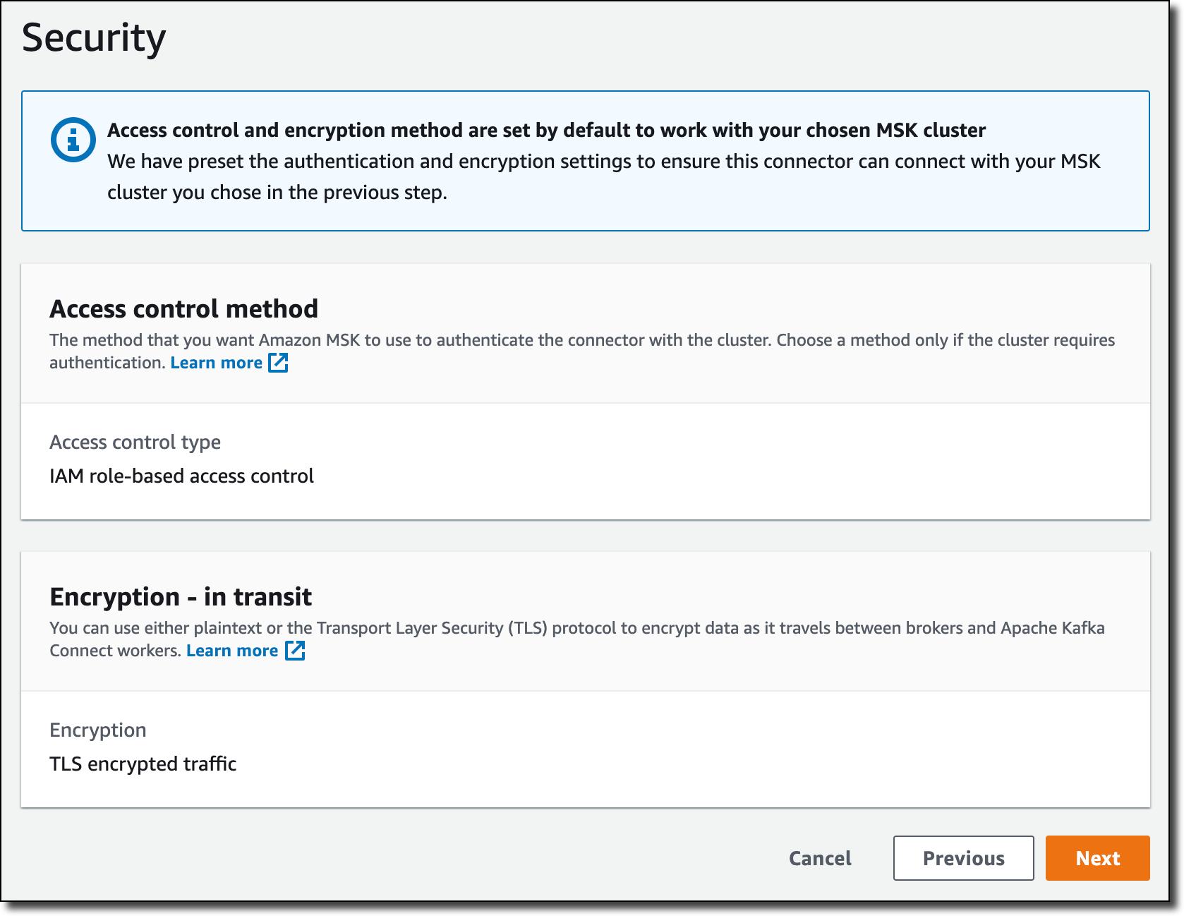
You now can launch the familiar RStudio Workbench with a simple click from Amazon SageMaker. Before getting started, your administrator needs to buy an appropriate license from RStudio PBC for end-users, set up your granted licenses in AWS License Manager, and create an Amazon SageMaker domain and user profile to launch RStudio on Amazon SageMaker. To learn all the administrator jobs, including managing licenses and monitoring usages, see a blog post of the setting up process, or Manage RStudio on Amazon SageMaker in the AWS documentation.

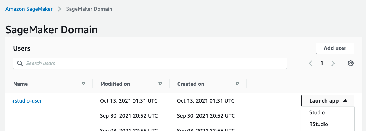
Once the required setup process is completed, you can open the RStudio Workbench from the new Launch app drop-down list in the created user list and select RStudio.

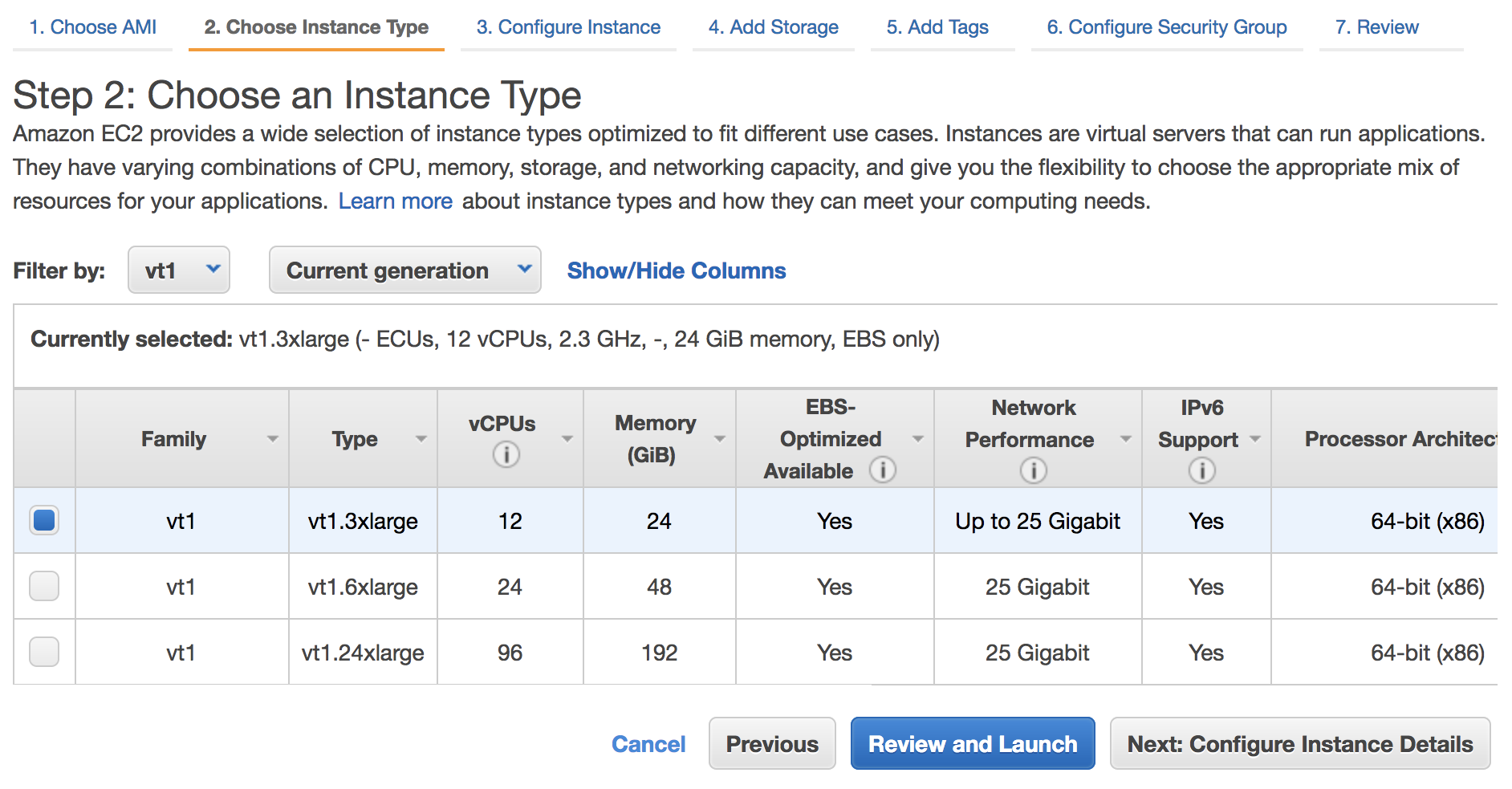
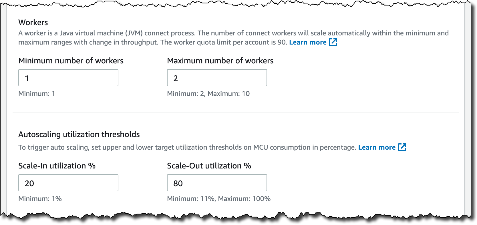
You will immediately see the RStudio Workbench home page and a list of sessions, projects, and published content on the home page. To create a new session, select the New Session button on the page, select a desired instance in the Instance Type dropdown list, and choose Start Session.

When you choose a compute instance type for a lightweight analysis that can be powered by two vCPU and four GiB memory, you can use a default ml.t3.medium instance. For a complex and large-scale ML modeling, you can choose a large instance with desired compute and memory from a wide array of ML instances available on Amazon SageMaker.

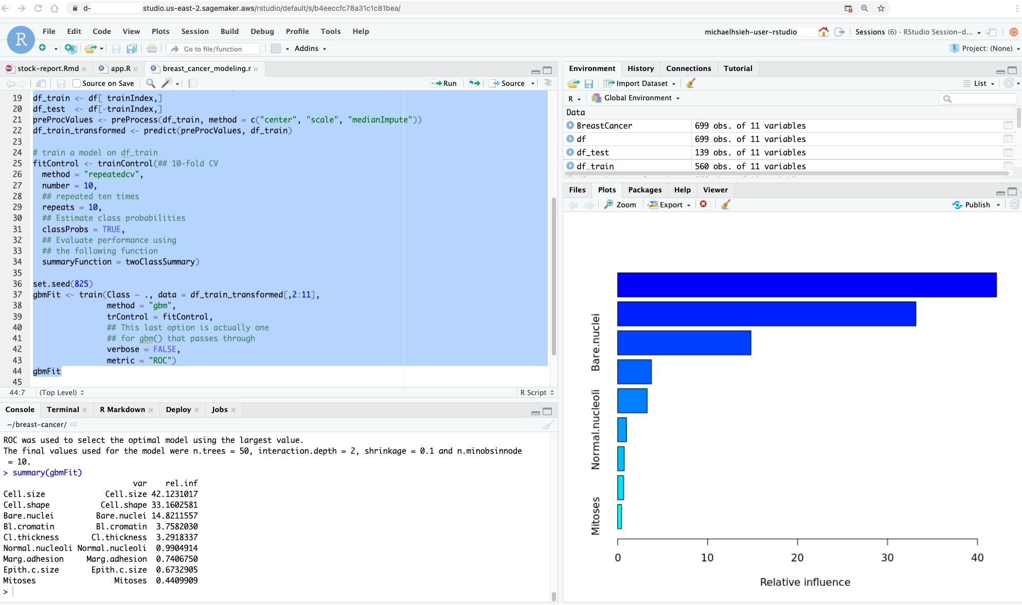
In a few minutes, your session will be ready for development in RStudio Workbench. When you launch your RStudio session, the Base R image serves as the basis of your instance. This Docker image includes R v4.0, AWS tools such as awscli, sagemaker, boto3 Python packages, and reticulate package for the interoperability between Python and R.

Managing R Packages and Publishing your Analysis
Along with the RStudio Workbench, RStudio Connect and RStudio Package Manager are the most used products of RStudio.

RStudio Connect is designed to allow data scientists to publish insights and dashboard and web applications from RStudio Workbench easily. RStudio Package Manager centrally manages the package repository for your organization so that data scientists can securely install packages faster while ensuring project reproducibility and repeatability.

Your administrator, for example, can create a repository and subscribe it to the built-in source named cran in RStudio Package Manager.

$ rspm sync --wait # Initiate a sync
$ rspm create repo --name=prod-cran --description='Access CRAN packages' # Create a repository:
$ rspm subscribe --repo=prod-cran --source=cran # Subscribe the repository to the cran source

When these steps are completed, you can use the prod-cran repository in the web interface of RStudio Package Manager.

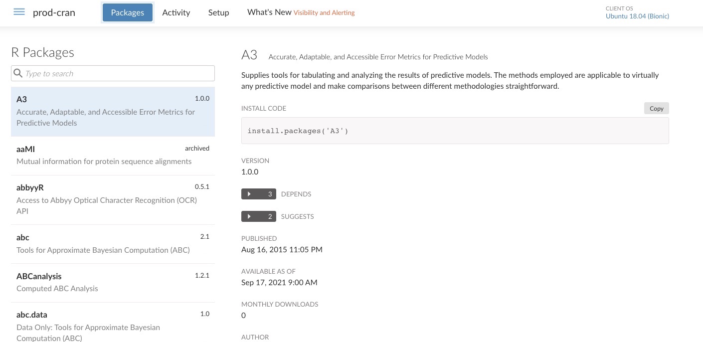
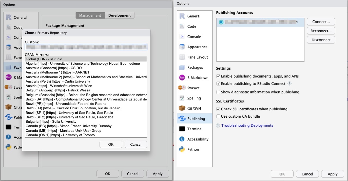
Now, you can configure this repository to install and manage your packages in RStudio Workbench. You can also configure RStudio Connect to publish insights, dashboard and web applications from RStudio Workbench via RStudio Connect so that your collaborators can easily consume your work.

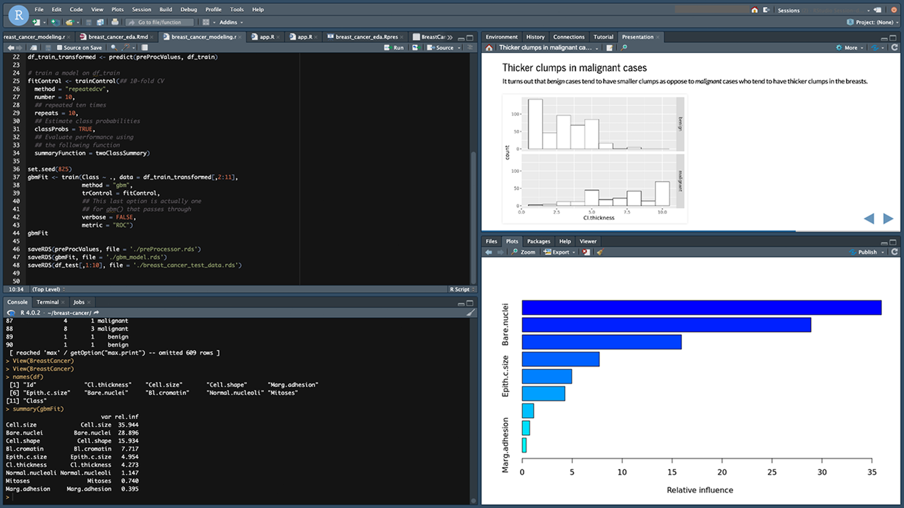
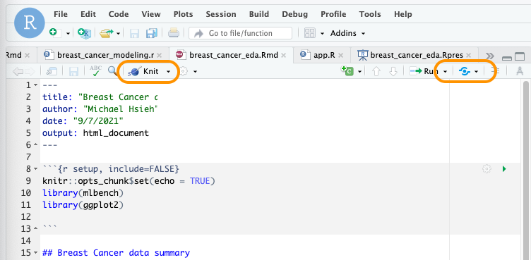
For example, you run the analysis inline to create an R Markdown that can be published to your collaborators. You can preview the slides while writing codes with the Preview button and publish it with the Publish icon in your RStudio session.

You can also publish Shiny application easy to create interactive web interfaces, or Python-based content such as Streamlit to the RStudio Connect instance.

To learn more, see Host RStudio Connect and Package Manager for ML development in RStudio on Amazon SageMaker written by my colleagues, Michael Hsieh, Chayan Panda, and Farooq Sabir on the AWS Machine Learning Blog.

Integrating training jobs with Amazon SageMaker
One of the benefits of using RStudio on Amazon SageMaker is the integration of Amazon SageMaker features. Your RStudio and Jupyter Notebook instances of Amazon SageMaker allow you to share the same Amazon EFS file system. You can import R codes written in Jupyter Notebook or use the same files in both Jupyter Notebook and RStudio without having to move your files between the two.

For example, you can run an R sample code including importing libraries, creating an Amazon SageMaker session, getting the IAM role, and importing and visualizing sample data. And then, it stores data on the S3 bucket, and triggers a training task with an XGBoost model by specifying the training container and defining an Amazon SageMaker Estimator. To learn more, see R sample codes in Amazon SageMaker.

# Import reticulate, readr and sagemaker libraries
library(reticulate)
library(readr)
sagemaker <- import('sagemaker')

# Create a sagemaker session
session <- sagemaker$Session()

# Get execution role
role_arn <- sagemaker$get_execution_role()

# Read a csv file from UCI public repository
data_file <- 'http://archive.ics.uci.edu/ml/machine-learning-databases/abalone/abalone.data'

# Copy data to a dataframe, rename columns, and show dataframe head
data_csv <- read_csv(file = data_file, col_names = FALSE, col_types = cols())
names(data_csv) <- c('sex', 'length', 'diameter', 'height', 'whole_weight', 'shucked_weight', 'viscera_weight', 'shell_weight', 'rings')
head(data_csv)

# Visualize data have height equal to 0
library(ggplot2)
options(repr.plot.width = 5, repr.plot.height = 4) 
ggplot(abalone, aes(x = height, y = rings, color = sex, alpha=0.5)) + geom_point() + geom_jitter()

# Upload data to Amazon S3 bucket
s3_train <- session$upload_data(path = data_csv,
                                bucket = my_s3_bucket, 
                                key_prefix = 'r_hello_world_demo/data')
s3_path = paste('s3://',bucket,'/r_hello_world_demo/data/abalone.csv',sep = '')

# Train a XGBoost model, specify the training containers, and define an Amazon SageMaker Estimator
container <- sagemaker$image_uris$retrieve(framework='xgboost', 
                                           region= session$boto_region_name, 
										   version='latest')							
estimator <- sagemaker$estimator$Estimator(image_uri = container,
                                           role = role_arn,
                                           train_instance_count = 1L,
                                           train_instance_type = 'ml.m5.4xlarge',
                                           train_volume_size = 30L,
                                           train_max_run = 3600L,
                                           input_mode = 'File',
                                           output_path = s3_path)

Now Available
RStudio on Amazon SageMaker is available in all AWS Regions where both Amazon SageMaker Studio and AWS License Manager are available. You can bring your own license of RStudio on Amazon SageMaker and pay for the underlying compute and storage resources within Amazon SageMaker or other AWS services, based on your usage.

To get started with RStudio on Amazon SageMaker, you can use AWS Free Tier. You can use 250 hours of ml.t3.medium instance on Amazon SageMaker Studio per month for the first two months. To learn more, see Amazon SageMaker Pricing page.

Give it a try, and please send us feedback either in the AWS forum for Amazon SageMaker or through your usual AWS support contacts.

Channy

New – Amazon EC2 C6i Instances Powered by the Latest Generation Intel Xeon Scalable Processors

Post Syndicated from Channy Yun original https://aws.amazon.com/blogs/aws/new-amazon-ec2-c6i-instances-powered-by-the-latest-generation-intel-xeon-scalable-processors/

We recently introduced Amazon EC2 M6i instances powered by the latest generation Intel® Xeon® Scalable processors with an all-core turbo frequency of 3.5 GHz, which offer customers up to 15% improvement in price performance compared to M5 instances.

Today, I am happy to announce the availability of the new compute-optimized Amazon EC2 C6i instances, which offer up to 15% improvement in price performance for a variety of workloads, versus comparable C5 instances. These instances are ideal for running compute-intensive workloads such as batch processing, machine learning, high-end gaming, high performance computing (HPC) workloads, ad serving, and video encoding.

Compared to C5 instances using an Intel processor, this new instance type provides:

  • Up to 15% improvement in compute price performance.
  • Up to 9% higher memory bandwidth.
  • Up to 40 Gbps for Amazon Elastic Block Store (EBS) and 50 Gbps for networking.
  • Always-on memory encryption.

Like M6i, C6i instances are available in 9 sizes:

Name vCPUs Memory
(GiB)
Network Bandwidth
(Gbps)
EBS Throughput
(Gbps)
c6i.large 2 4 Up to 12.5 Up to 10
c6i.xlarge 4 8 Up to 12.5 Up to 10
c6i.2xlarge 8 16 Up to 12.5 Up to 10
c6i.4xlarge 16 32 Up to 12.5 Up to 10
c6i.8xlarge 32 64 12.5 10
c6i.12xlarge 48 96 18.75 15
c6i.16xlarge 64 128 25 20
c6i.24xlarge 96 192 37.5 30
c6i.32xlarge 128 256 50 40

The new instances are built on the AWS Nitro System, a collection of building blocks that offloads many of the traditional virtualization functions to dedicated hardware for high performance, high availability, and highly secure cloud instances.

As you should do with M6i instances, for optimal networking performance, upgrade your Elastic Network Adapter (ENA) drivers to version 3. For more information, see this article about migrating an EC2 instance to a sixth-generation instance in the AWS Knowledge Center.

C6i instances support Elastic Fabric Adapter (EFA) on the c6i.32xlarge size for workloads that can benefit from lower network latency, such as HPC and video processing.

Available Now
C6i instances are available today in four AWS Regions: US East (N. Virginia, Ohio), US West (Oregon), and EU (Ireland). As usual with EC2, you pay for what you use. For more information, see the EC2 pricing page.

To learn more, visit the EC2 C6i instance page. You can send feedback to the AWS forum for Amazon EC2 or through your usual AWS Support contacts.

Channy

Goodbye Microsoft SQL Server, Hello Babelfish

Post Syndicated from Sébastien Stormacq original https://aws.amazon.com/blogs/aws/goodbye-microsoft-sql-server-hello-babelfish/

Many of our customers are telling us they want to move away from commercial database vendors to avoid expensive costs and burdensome licensing terms. But migrating away from commercial and legacy databases can be time-consuming and resource-intensive. When migrating your databases, you can automate the migration of your database schema and data using the AWS Schema Conversation Tool and AWS Database Migration Service. But there is always more work to do to migrate the application itself, including rewriting application code that interacts with the database. Motivation is there, but costs and risks are often limiting factors.

Today, we are making Babelfish for Aurora PostgreSQL available. Babelfish allows Amazon Aurora PostgreSQL-Compatible Edition to understand the SQL Server wire protocol. It allows you to migrate your SQL Server applications to PostgreSQL cheaper, faster, and with less risks involved with such change.

You can migrate your application in a fraction of the time that a traditional migration would require. You continue to use the existing queries and drivers your application uses today. Just point the application to an Amazon Aurora PostgreSQL database with Babelfish activated. Babelfish adds the capability to Amazon Aurora PostgreSQL to understand the SQL Server wire protocol Tabular Data Stream (TDS), as well as extending PostgreSQL to understand commonly used T-SQL commands used by SQL Server. Support for T-SQL includes elements such as the SQL dialect, static cursors, data types, triggers, stored procedures, and functions. Babelfish reduces the risk associated with database migration projects by significantly reducing the number of changes required to the application. When adopting Babelfish, you save on licensing costs of using SQL Server. Amazon Aurora provides the security, availability, and reliability of commercial databases at 1/10th the cost.

SQL Server has evolved over more than 30 years, and we do not expect to support all functionalities right away. Instead, we focused on the most common T-SQL commands and returning the correct response or an error message. For example, the MONEY datatype has different characteristics in SQL Server (with four decimals precision) and PostgreSQL (with two decimals precision). Such a subtle difference might lead to rounding errors and have a significant impact on downstream processes, such as financial reporting. In this case, and many others, Babelfish ensures the semantics of SQL Server data types and T-SQL functionality are preserved: we created a MONEY datatype that behaves as SQL Server apps would expect. When you create a table with this datatype through the Babelfish connection, you get this compatible datatype and behaviors that a SQL Server app would expect.

Create a Babelfish Cluster Using the Console
To show you how Babelfish works, let’s first connect to the console and create a new Amazon Aurora PostgreSQL cluster. The procedure is no different than for the regular Amazon Aurora database. In the RDS launch wizard, I first make sure I select an Aurora version compatible with PostgreSQL 13.4, or more recent. The updated console has additional filters to help you select the versions that are compatible with Babelfish.

Babelfish Create databaseThen, lower on the page, I select the option Turn on Babelfish.

Aurora turn on babelfish

Under Monitoring section, I also make sure I turn off Enable Enhanced monitoring. This option requires additional IAM permissions and preparation that are not relevant for this demo.

Enable Enhanced MonitoringAfter a couple of minutes, my cluster is created, it has two instances, one writer and one reader.

Babelfish cluster created

Create a Babelfish Cluster Using the CLI
Alternatively, I may use the CLI to create a cluster. I first create a parameter group to activate Babelfish (the console does it automatically):

aws rds create-db-cluster-parameter-group             \
    --db-cluster-parameter-group-name myapp-babelfish \
    --db-parameter-group-family aurora-postgresql13   \
    --description "babelfish APG 13"
aws rds modify-db-cluster-parameter-group             \
    --db-cluster-parameter-group-name myapp-babelfish \
    --parameters "ParameterName=rds.babelfish_status,ParameterValue=on,ApplyMethod=pending-reboot" \

Then I create the database cluster (when using the command below, adjust the security group id and the subnet group name) :

aws rds create-db-cluster \
    --db-cluster-identifier awsnewblog-cli-demo \
    --master-username postgres \  
    --master-user-password Passw0rd \
    --engine aurora-postgresql \
    --engine-version 13.4 \
    --vpc-security-group-ids sg-abcd1234 \
    --db-subnet-group-name default-vpc-1234abcd \
    --db-cluster-parameter-group-name myapp-babelfish
{
    "DBCluster": {
        "AllocatedStorage": 1,
        "AvailabilityZones": [
            "us-east-1c",
            "us-east-1d",
            "us-east-1a"
        ],
        "BackupRetentionPeriod": 1,
        "DBClusterIdentifier": "awsnewblog-cli-demo",
        "Status": "creating",
        ... <redacted for brevity> ...
    }
}

Once the cluster is created, I create an instance using

aws rds create-db-instance \
    --db-instance-identifier myapp-db1 \
    --db-instance-class db.r5.4xlarge \
    --db-subnet-group-name default-vpc-1234abcd \
    --db-cluster-identifier awsnewblog-cli-demo \
    --engine aurora-postgresql
{
    "DBInstance": {
        "DBInstanceIdentifier": "myapp-db1",
        "DBInstanceClass": "db.r5.4xlarge",
        "Engine": "aurora-postgresql",
        "DBInstanceStatus": "creating",
        ... <redacted for brevity> ...

Connect to the Babelfish Cluster
Once the cluster and instances are ready, I connect to the writer instance to create the database itself. I may connect to the instance using SQL Server Management Studio (SSMS) or other SQL client such as sqlcmd. The Windows client must be able to connect to the Babelfish cluster, I made sure the RDS security group authorizes connections from the Windows host.

Using SSMS on Windows, I select New Query in the toolbar, I enter the database DNS name as Server name. I select SQL Server Authentication and I enter the database Login and Password. I click on Connect.

Important: Do not connect via the SSMS Object Explorer. Be sure to connect using the query editor via the New Query button. At this time, Babelfish supports the query editor, but not the Object Explorer.

SSMS Connect to babelfish

Once connected, I check the version with select @@version statement and click the green Execute button in the toolbar. I can read the statement result on the bottom part of the screen.

Babelfish check version

Finally, I create the database on the instance with the create database demo statement.

babelfish create database

By default, Babelfish runs in single-db mode. Using this mode, you can have maximum one user database per instance. It allows to have a close mapping of schema names between SQL Server and PostgreSQL. Alternatively, you may turn on multi-db mode at cluster creation time. This allows you to create multiple user databases per instance. In PostgreSQL, user databases will be mapped to multiple schemas with the database name as a prefix.

Run an Application
For the purpose of this demo, I use a database schema provided by SQLServerTutorial.net as part of their SQL Server Tutorial to create a schema and populate it with data. The SQL script and application C# code I use in this demo are available on my GitHub repository. A big thanks to my colleague Anuja for providing me with a C# demo application.

In SQL Server Management Studio, I open the create_objects.sql script and I choose the green execute icon on the top toolbar. A confirmation message tells me the database schema is created.

babelfish create schema

I repeat the operation with the load_data.sql script to load data in the newly created tables. Data loading takes a few minutes to run.

Now the database is loaded, let’s open Anuja‘s  C# application developed to access a SQL Server database. I modify two lines of code:

  • line 12 : I type the DNS name of the Babelfish cluster I created earlier. Note that I use the DNS name of a “write” node from my cluster.
  • line 15 : I type the password I entered when I created the database cluster.

Visual Studio Code - Prepare app to connect to babelfish

And that’s it! No other modification is required on this app. This code written to query and interact with SQL Server is just working “as-is” on Aurora PostgreSQL with Babelfish.

babelfish application execution

Open Source Transparency
We decided to open-source the technology behind Babelfish to create the Babelfish for PostgreSQL open source project. It uses the permissive Apache 2.0 and PostgreSQL licenses, meaning you can modify or tweak or distribute Babelfish in whatever fashion you see fit. Over time, we are shifting Babelfish to fully open development on GitHub, so there is transparency from the start. Now, anyone, whether you are an AWS customer or not, can use Babelfish to leave behind SQL Server and quickly, easily, and cost-effectively migrate your applications to open source PostgreSQL. We believe Babelfish is going to make PostgreSQL accessible to a much wider group of customers and developers than ever before, particularly those with large numbers of complex applications originally written for SQL Server.

Availability
Babelfish for Aurora PostgreSQL is available today in all publicly available AWS Regions at no additional cost. Start your application migration today.

— seb

PS : if you wonder where the name Babelfish comes from, just remember the answer is 42. (Or you can read this slightly longer answer.)

New – Attribute-Based Instance Type Selection for EC2 Auto Scaling and EC2 Fleet

Post Syndicated from Danilo Poccia original https://aws.amazon.com/blogs/aws/new-attribute-based-instance-type-selection-for-ec2-auto-scaling-and-ec2-fleet/

The first AWS service I used, more than ten years ago, was Amazon Elastic Compute Cloud (Amazon EC2). Over time, EC2 has added a wide selection of instance types optimized to fit different use cases, with a varying combination of CPU/GPU, memory, storage, and networking capacity to give you the flexibility to choose the appropriate mix of resources for your applications.

One of the key advantages of the cloud is elasticity. With EC2 Fleet, you can synchronously request capacity across multiple instance types and purchase options, launching your instances across multiple Availability Zones, using the On-Demand, Reserved, and Spot Instances together. With EC2 Auto Scaling, you can automatically add or remove EC2 instances according to conditions you define and add advanced instance management capabilities such as warm pools, instance refresh, and health checks. With these tools, you need to manually update your configurations to benefit from the newest EC2 instances. Also, when you use EC2 Spot Instances to optimize your costs, it is important that you select multiple instance types to access the highest amount of Spot capacity. Until now, there was no easy way to build and maintain instance type configurations in a flexible way.

Today, I am happy to share that we are introducing attribute-based instance type selection (ABS), a new feature that lets you express your instance requirements as a set of attributes, such as vCPU, memory, and storage. Your requirements are translated by ABS to all matching instance types, simplifying the creation and maintenance of instance type configurations. This also allows you to automatically use newer generation instance types when they are released and access a broader range of capacity via EC2 Spot Instances. EC2 Fleet and EC2 Auto Scaling select and launch instances that fit the specified attributes, removing the need to manually pick instance types.

ABS is ideal for flexible workloads and frameworks, such as when running containers or web fleets, processing big data, and implementing continuous integration and deployment (CI/CD) tooling. When using Spot Instances, instead of picking and entering tens of instance types and sizes, you can now just use a simple attribute config to cover all of them and include new ones as they come out.

How Attribute-Based Instance Type Selection Works
With ABS, you replace the list of instance types with your instance requirements. You can specify instance requirements inside a launch template or in the EC2 Fleet or EC2 Auto Scaling requests as a launch template override.

ABS works in two steps:

  • First, ABS determines a list of instance types based on specified attributes, AWS Region, Availability Zone, and price.
  • Then, EC2 Auto Scaling or EC2 Fleet applies the selected allocation strategy to that list.

For Spot Instances, ABS supports the capacity-optimized and the lowest-price allocation strategies.

For On-Demand Instances, ABS supports the lowest-price allocation strategy. EC2 Auto Scaling or EC2 Fleet will resolve ABS attributes to a list of instance types and will launch the lowest priced instance first to fulfill the On-Demand portion of the capacity request, moving to the next lowest priced instance if needed.

By default ABS enables price protection to keep your spending under control. Price protection makes ABS avoid provisioning overly expensive instance types even if they happen to fit the attributes you selected and keeps the prices of provisioned instances within certain boundaries. With price protection enabled, ABS doesn’t select instance types whose price is above price protection thresholds. There are two separate thresholds for Spot and On-Demand instances that you can optionally customize.

Let’s see how ABS works in practice with a couple of examples.

Using Attribute-Based Instance Type Selection with EC2 Auto Scaling
I use the AWS Command Line Interface (CLI) with the --generate-cli-skeleton parameter to generate a file in YAML format with all the parameters accepted by the CreateAutoScalingGroup API.

aws autoscaling create-auto-scaling-group \
    --generate-cli-skeleton yaml-input > create-asg.yaml

In the YAML file, there is a new InstanceRequirements section that can be used to override the configuration of the launch template. These are all the attributes I can choose from with some sample values:

InstanceRequirements:
  VCpuCount:  # [REQUIRED] 
    Min: 0
    Max: 0
  MemoryMiB: # [REQUIRED] 
    Min: 0
    Max: 0
  CpuManufacturers:
  - amd
  MemoryGiBPerVCpu:
    Min: 0.0
    Max: 0.0
  ExcludedInstanceTypes:
  - ''
  InstanceGenerations:
  - previous
  SpotMaxPricePercentageOverLowestPrice: 0
  OnDemandMaxPricePercentageOverLowestPrice: 0
  BareMetal: required  #  Valid values are: included, excluded, required.
  BurstablePerformance: excluded #  Valid values are: included, excluded, required.
  RequireHibernateSupport: true
  NetworkInterfaceCount:
    Min: 0
    Max: 0
  LocalStorage: required  #  Valid values are: included, excluded, required.
  LocalStorageTypes:
  - ssd
  TotalLocalStorageGB:
    Min: 0.0
    Max: 0.0
  BaselineEbsBandwidthMbps:
    Min: 0
    Max: 0
  AcceleratorTypes:
  - inference
  AcceleratorCount:
    Min: 0
    Max: 0
  AcceleratorManufacturers:
  - amazon-web-services
  AcceleratorNames:
  - a100
  AcceleratorTotalMemoryMiB:
    Min: 0
    Max: 0

Instead of providing a list of overrides, each having an InstanceType attribute with a single instance type selected, I can now select the instance types based on my requirements. I can specify the minimum and maximum amount of vCPUs, and the range of memory. Optionally, I can ask for a minimum amount of memory per vCPUs.

There are many more attributes that I can select from. For example, I can include, exclude, or require the use of bare metal or burstable instances. I can add networking or storage requirements. If necessary, I can ask for GPU or FPGA accelerators, and so on.

In my case, I ask for instances with two to four vCPUs and at least 2048 MiB of memory. Previously, it would have taken about 40 overrides, one for each instance type that meets these requirements, but with ABS, I just have to specify three parameters in the InstanceRequirements section. This is the full configuration file I am going to use to create the Auto Scaling group:

AutoScalingGroupName: 'my-asg' # [REQUIRED] 
MixedInstancesPolicy:
  LaunchTemplate:
    LaunchTemplateSpecification:
      LaunchTemplateId: 'lt-0537239d9aef10a77'
    Overrides:
    - InstanceRequirements:
        VCpuCount: # [REQUIRED] 
          Min: 2
          Max: 4
        MemoryMiB: # [REQUIRED] 
          Min: 2048
  InstancesDistribution:
    OnDemandPercentageAboveBaseCapacity: 50
    SpotAllocationStrategy: 'capacity-optimized'
MinSize: 0 # [REQUIRED] 
MaxSize: 100 # [REQUIRED] 
DesiredCapacity: 4
VPCZoneIdentifier: 'subnet-e76a128a,subnet-e66a128b,subnet-e16a128c'

I create the Auto Scaling group passing the configuration file with the --cli-input-yaml parameter:

aws autoscaling create-auto-scaling-group \
    --cli-input-yaml file://my-create-asg.yaml

After a few minutes, four EC2 instances (corresponding to my DesiredCapacity) are running in the EC2 console. In the list, I find both C3 and C5a instances, spanning both time and CPU manufacturer.

Console screenshot.

Of those instances, 50 percent is On-Demand (based on the OnDemandPercentageAboveBaseCapacity option in the InstancesDistribution section). In the Spot Request tab of the EC2 console, I see the two requests:

Console screenshot.

As expected, all instance types follow my requirements and have size large. However, I quickly realize my application needs more compute capacity in each instance. I update the Auto Scaling group with the new requirements, asking for more vCPUs (between four and six):

aws autoscaling update-auto-scaling-group \
    --auto-scaling-group-name my-asg \
    --mixed-instances-policy '{
        "LaunchTemplate": {
            "Overrides": [
                {
                    "InstanceRequirements": {
                    "VCpuCount":{"Min": 4, "Max": 6},
                    "MemoryMiB":{"Min": 2048} }
                } ]
        } }' 

Then, I start the instance refresh of the Auto Scaling group:

aws autoscaling start-instance-refresh \
    --auto-scaling-group-name my-asg

EC2 Auto Scaling performs a rolling replacement of the instances based on the new requirements. After a few minutes, all instances have been replaced by new ones with size xlarge, and I have a mix of C5, C5a, and M3 instances running. All previous instances have been terminated.

Console screenshot.

Similar to before, two of the new instances are launched using Spot requests. The previous Spot requests have been closed.

Console screenshot.

How to Preview Matching Instances without Launching Them
To better understand how the new ABS works, I use the new EC2 GetInstanceTypesFromInstanceRequirements API. This API returns the list of instance types matching my requirements.

First, I create the YAML parameter file:

aws ec2 get-instance-types-from-instance-requirements --generate-cli-skeleton yaml-input > requirements.yaml

I edit the file with the same requirements I used to update the Auto Scaling group. This time, I also ask to use current generation instances:

ArchitectureTypes:  # [REQUIRED] 
- x86_64
VirtualizationTypes: # [REQUIRED] 
- hvm
InstanceRequirements: # [REQUIRED] 
  VCpuCount:
    Min: 4
    Max: 6
  MemoryMiB:
    Min: 2048
  InstanceGenerations:
    - current

Note that here I had to specify the type of architecture (x86_64) and virtualization (hvm). When creating the Auto Scaling group, this information was provided by the Amazon Machine Images (AMI) used by the launch template.

Now, let’s preview all the instance types selected by these requirements:

aws ec2 get-instance-types-from-instance-requirements \
    --cli-input-yaml file://requirements.yaml \
    --output table

------------------------------------------
|GetInstanceTypesFromInstanceRequirements|
+----------------------------------------+
||             InstanceTypes            ||
|+--------------------------------------+|
||             InstanceType             ||
|+--------------------------------------+|
||  c4.xlarge                           ||
||  c5.xlarge                           ||
||  c5a.xlarge                          ||
||  c5ad.xlarge                         ||
||  c5d.xlarge                          ||
||  c5n.xlarge                          ||
||  d2.xlarge                           ||
||  d3.xlarge                           ||
||  d3en.xlarge                         ||
||  g3s.xlarge                          ||
||  g4ad.xlarge                         ||
||  g4dn.xlarge                         ||
||  i3.xlarge                           ||
||  i3en.xlarge                         ||
||  inf1.xlarge                         ||
||  m4.xlarge                           ||
||  m5.xlarge                           ||
||  m5a.xlarge                          ||
||  m5ad.xlarge                         ||
||  m5d.xlarge                          ||
||  m5dn.xlarge                         ||
||  m5n.xlarge                          ||
||  m5zn.xlarge                         ||
||  m6i.xlarge                          ||
||  p2.xlarge                           ||
||  r4.xlarge                           ||
||  r5.xlarge                           ||
||  r5a.xlarge                          ||
||  r5ad.xlarge                         ||
||  r5b.xlarge                          ||
||  r5d.xlarge                          ||
||  r5dn.xlarge                         ||
||  r5n.xlarge                          ||
||  x1e.xlarge                          ||
||  z1d.xlarge                          ||
|+--------------------------------------+|

Using this new EC2 API, I can quickly test different requirements and see how they map to instance types. When new instance types are released, they are automatically added to the list if they match my requirements.

Availability and Pricing
You can use attribute-based instance type selection (ABS) with EC2 Auto Scaling and EC2 Fleet today in all public and GovCloud AWS Regions, with the exception of those based in China where we need more time. You can configure ABS using the AWS Command Line Interface (CLI), AWS SDKs, AWS Management Console, and AWS CloudFormation. There is no additional charge for using ABS; you only pay the standard EC2 pricing for the provisioned instances. For more information on price protection, see the EC2 Auto Scaling documentation.

This new feature makes it easy to use flexible instance type configurations instead of long lists of instance types. In this way, you can automatically use newer generation instance types when they are released in the Region. Also, you can easily access more capacity with your Spot requests.

Simplify your EC2 instance type configurations with attribute-based instance type selection.

Danilo

New – EC2 Instances Powered by Gaudi Accelerators for Training Deep Learning Models

Post Syndicated from Jeff Barr original https://aws.amazon.com/blogs/aws/new-ec2-instances-powered-by-gaudi-accelerators-for-training-deep-learning-models/

There are more applications today for deep learning than ever before. Natural language processing, recommendation systems, image recognition, video recognition, and more can all benefit from high-quality, well-trained models.

The process of building such a model is iterative: construct an initial model, train it on the ground truth data, do some test inferences, refine the model and repeat. Deep learning models contain many layers (hence the name), each of which transforms outputs of the previous layer. The training process is math and processor intensive, and places demands on just about every part of the systems used for training including the GPU or other training accelerator, the network, and local or network storage. This sophistication and complexity increases training time and raises costs.

New DL1 Instances
Today I would like to tell you about our new DL1 instances. Powered by Gaudi accelerators from Habana Labs, the dl1.24xlarge instances have the following specs:

Gaudi Accelerators – Each instance is equipped with eight Gaudi accelerators, with a total of 256 GB of High Bandwidth (HBM2) accelerator memory and high-speed, RDMA-powered communication between accelerators.

System Memory – 768 GB of system memory, enough to hold very large sets of training data in memory, as often requested by our customers.

Local Storage – 4 TB of local NVMe storage, configured as four 1 TB volumes.

Processor – Intel Cascade Lake processor with 96 vCPUs.

Network – 400 Gbps of network throughput.

As you can see, we have maxed out the specs in just about every dimension, with the goal of giving you a highly capable machine learning training platform with a low cost of entry and up to 40% better price-performance than current GPU-based EC2 instances.

Gaudi Inside
The Gaudi accelerators are custom-designed for machine learning training, and have a ton of cool & interesting features & attributes:

Data Types – Support for floating point (BF16 and FP32), signed integer (INT8, INT16, and INT32), and unsigned integer (UINT8, UINT16, and UINT32) data.

Generalized Matrix Multiplier Engine (GEMM) – Specialized hardware to accelerate matrix multiplication.

Tensor Processing Cores (TPCs) – Specialized VLIW SIMD (Very Long Instruction Word / Single Instruction Multiple Data) processing units designed for ML training. The TPCs are C-programmable, although most users will use higher-level tools and frameworks.

Getting Started with DL1 Instances
The Gaudi SynapseAI Software Suite for Training will help you to build new models and to migrate existing models from popular frameworks such as PyTorch and TensorFlow:

Here are some resources to get you started:

TensorFlow User Guide – Learn how to run your TensorFlow models on Gaudi.

PyTorch User Guide – Learn how to run your PyTorch models on Gaudi.

Gaudi Model Migration Guide – Learn how to port your PyTorch or TensorFlow to Gaudi.

HabanaAI Repo – This large, active repo contains setup instructions, reference models, academic papers, and much more.

You can use the TPC Programming Tools to write, simulate, and debug code that runs directly on the TPCs, and you can use the Habana Communication Library (HCL) to build applications that harness the power of multiple accelerators. The Habana Collective Communications Library (HCCL) runs atop HCL and gives you access to collective primitives for Reduce, Broadcast, Gather, and Scatter operations.

Now Available
DL1 instances are available today in the US East (N. Virginia) and US West (Oregon) Regions in On-Demand and Spot form. You can purchase Reserved Instances and Savings plans as well.

Jeff;

AWS Local Zones Are Now Open in Las Vegas, New York City, and Portland

Post Syndicated from Sébastien Stormacq original https://aws.amazon.com/blogs/aws/aws-local-zones-are-now-open-in-las-vegas-new-york-city-and-portland/

Today, we are opening three new AWS Local Zones in Las Vegas, New York City (located in New Jersey), and Portland metro areas. We are now at a total of 14 Local Zones in 13 cities since Jeff Barr announced the first Local Zone in Los Angeles in December 2019. These three new Local Zones join the ones in full operation in Boston, Chicago, Dallas, Denver, Houston, Kansas City, Los Angeles, Miami, Minneapolis, and Philadelphia.

Local Zones are one of the ways we bring select AWS services much closer to large populations and geographic areas where major industries come together. By having this proximity, you can deploy latency-sensitive workloads such as real-time gaming platforms, financial transaction processing, media and entertainment content creation, or ad services. Using Local Zones for migrations or hybrid strategies are two additional use cases allowing you to migrate your applications to a nearby AWS Local Zone while still meeting the low-latency requirements of hybrid deployments.

Local Zones support the deployment of workloads using Amazon Elastic Compute Cloud (Amazon EC2), Amazon Elastic Block Store (EBS), Amazon FSx for Windows File Server and Amazon FSx for Lustre, Elastic Load Balancing, Amazon Relational Database Service (RDS), and Amazon Virtual Private Cloud (VPC). Local Zones provide a high-bandwidth, secure connection between local workloads and those running in the parent AWS Region, while offering the full range of services found in a Region through the same APIs, console and tool sets. This page lists the exact AWS services and features available in each Local Zone.

Local Zones are easy to use and can be enabled in only three clicks! This article will help you learn how to provision infrastructure in a Local Zone, which is very similar to creating infrastructure in an Availability Zone. Once enabled, Local Zones appear as additional Availability Zones in your AWS Management Console or AWS Command Line Interface (CLI).

Local Zones in Action
Examples of workloads that our customers run in Local Zones include:

Dish Wireless is building the US-telecom’s first cloud-native 5G network. They are unleashing 5G connectivity with better speed, better security, and better latency. DISH is leveraging AWS Regions, AWS Local Zones, and AWS Outposts to extend AWS infrastructure and services to wherever they – or their customers – need it.

Integral Ad Science (IAS) is a global leader in digital media quality. Every millisecond counts when it comes to delivering actionable insights for its advertiser and publisher customers. Leveraging AWS Regions and AWS Local Zones, IAS ensures rapid response times in milliseconds when analyzing data and delivering insights.

Esports Engine (a Vindex company) is a turnkey esports solutions company working with gaming publishers, rights holders, brands, and teams to provide production, broadcast, tournament, and program design. Their graphic-intensive streaming content is live-fed from the locations where the games are recorded and then broadcast from the studios to viewers. AWS Local Zones replace their previous on-premises data centers to reduce the need for support for the physical data center buildings.

Proof Trading is a financial services company looking forward to taking advantage of AWS Local Zones to bring trading workloads closer to the major trading venues located in Chicago and New Jersey. Our industry blog has a detailed article that provides more context on trading-related workloads.

Ubitus is a cloud gaming technology leader. They deploy latency-sensitive game servers all over the world to be closer to gamers. An important part of having a great gaming experience is to have consistent low-latency game plays. AWS Local Zones are a game changer for them. Now, they can easily deploy and test clusters of game servers in many cities across the US, ensuring that more customers get a consistent experience regardless of where they are located.

What’s Next?
In 2019 when we launched our first Local Zone at AWS re:Invent 2019, we said we were just getting started. In addition to today’s announcement, we are working on opening three additional Local Zones in Atlanta, Phoenix, and Seattle by the end of the year, and we keep expanding. If you would like to express your interest in a particular location, please let us know by filling out the AWS Local Zones Interest form.

We are also listening to your feedback on additional services that we should add to Local Zones, such as more EC2 instance types to give you even more flexibility.

Build and deploy your workload on a Local Zone today.

— seb

Amazon RDS Custom for Oracle – New Control Capabilities in Database Environment

Post Syndicated from Channy Yun original https://aws.amazon.com/blogs/aws/amazon-rds-custom-for-oracle-new-control-capabilities-in-database-environment/

Managing databases in self-managed environments such as on premises or Amazon Elastic Compute Cloud (Amazon EC2) requires customers to spend time and resources doing database administration tasks such as provisioning, scaling, patching, backups, and configuring for high availability. So, hundreds of thousands of AWS customers use Amazon Relational Database Service (Amazon RDS) because it automates these undifferentiated administration tasks.

However, there are some legacy and packaged applications that require customers to make specialized customizations to the underlying database and the operating system (OS), such as Oracle industry specialized applications for healthcare and life sciences, telecom, retail, banking, and hospitality. Customers with these specific customization requirements cannot get the benefits of a fully managed database service like Amazon RDS, and they end up deploying their databases on premises or on EC2 instances.

Today, I am happy to announce the general availability of Amazon RDS Custom for Oracle, new capabilities that enable database administrators to access and customize the database environment and operating system. With RDS Custom for Oracle, you can now access and customize your database server host and operating system, for example by applying special patches and changing the database software settings to support third-party applications that require privileged access.

You can easily move your existing self-managed database for these applications to Amazon RDS and automate time-consuming database management tasks, such as software installation, patching, and backups. Here is a simple comparison of features and responsibilities between Amazon EC2, RDS Custom for Oracle, and RDS.

Features and Responsibilities Amazon EC2 RDS Custom for Oracle Amazon RDS
Application optimization Customer Customer Customer
Scaling/high availability Customer Shared AWS
DB backups Customer Shared AWS
DB software maintenance Customer Shared AWS
OS maintenance Customer Shared AWS
Server maintenance AWS AWS AWS

The shared responsibility model of RDS Custom for Oracle gives you more control than in RDS, but also more responsibility, similar to EC2. So, if you need deep control of your database environment where you take responsibility for changes that you make and want to offload common administration tasks to AWS, RDS Custom for Oracle is the recommended deployment option over self-managing databases on EC2.

Getting Started with Amazon RDS Custom for Oracle
To get started with RDS Custom for Oracle, you create a custom engine version (CEV), the database installation files of supported Oracle database versions and upload the CEV to Amazon Simple Storage Service (Amazon S3). This launch includes Oracle Enterprise Edition allowing Oracle customers to use their own licensed software with bring your own license (BYOL).

Then with just a few clicks in the AWS Management Console, you can deploy an Oracle database instance in minutes. Then, you can connect to it using SSH or AWS Systems Manager.

Before creating and connecting your DB instance, make sure that you meet some prerequisites such as configuring the AWS Identity and Access Management (IAM) role and Amazon Virtual Private Cloud (VPC) using the pre-created AWS CloudFormation template in the Amazon RDS User Guide.

A symmetric AWS Key Management Service (KMS) key is required for RDS Custom for Oracle. If you don’t have an existing symmetric KMS key in your account, create a KMS key by following the instructions in Creating keys in the AWS KMS Developer Guide.

The Oracle Database installation files and patches are hosted on Oracle Software Delivery Cloud. If you want to create a CEV, search and download your preferred version under the Linux x86/64 platform and upload it to Amazon S3.

$ aws s3 cp install-or-patch-file.zip \ s3://my-oracle-db-files

To create CEV for creating a DB instance, you need a CEV manifest, a JSON document that describes installation .zip files stored in Amazon S3. RDS Custom for Oracle will apply the patches in the order in which they are listed when creating the instance by using this CEV.

{
    "mediaImportTemplateVersion": "2020-08-14",
    "databaseInstallationFileNames": [
        "V982063-01.zip"
    ],
    "opatchFileNames": [
        "p6880880_190000_Linux-x86-64.zip"
    ],
    "psuRuPatchFileNames": [
        "p32126828_190000_Linux-x86-64.zip"
    ],
    "otherPatchFileNames": [
        "p29213893_1910000DBRU_Generic.zip",
        "p29782284_1910000DBRU_Generic.zip",
        "p28730253_190000_Linux-x86-64.zip",
        "p29374604_1910000DBRU_Linux-x86-64.zip",
        "p28852325_190000_Linux-x86-64.zip",
        "p29997937_190000_Linux-x86-64.zip",
        "p31335037_190000_Linux-x86-64.zip",
        "p31335142_190000_Generic.zip"
] }

To create a CEV in the AWS Management Console, choose Create custom engine version in the Custom engine version menu.

You can set Engine type to Oracle, choose your preferred database edition and version, and enter CEV manifest, the location of the S3 bucket that you specified. Then, choose Create custom engine version. Creation takes approximately two hours.

To create your DB instance with the prepared CEV, choose Create database in the Databases menu. When you choose a database creation method, select Standard create. You can set Engine options to Oracle and choose Amazon RDS Custom in the database management type.

In Settings, enter a unique name for the DB instance identifier and your master username and password. By default, the new instance uses an automatically generated password for the master user. To learn more in the remaining setting, see Settings for DB instances in the Amazon RDS User Guide. Choose Create database.

Alternatively, you can create a CEV by running create-custom-db-engine-version command in the AWS Command Line Interface (AWS CLI).

$ aws rds create-db-instances \
      --engine my-oracle-ee \
      --db-instance-identifier my-oracle-instance \ 
      --engine-version 19.my_cev1 \ 
      --allocated-storage 250 \ 
      --db-instance-class db.m5.xlarge \ 
      --db-subnet-group mydbsubnetgroup \ 
      --master-username masterawsuser \ 
      --master-user-password masteruserpassword \ 
      --backup-retention-period 3 \ 
      --no-multi-az \ 
              --port 8200 \
      --license-model bring-your-own-license \
      --kms-key-id my-kms-key

After you create your DB instance, you can connect to this instance using an SSH client. The procedure is the same as for connecting to an Amazon EC2 instance. To connect to the DB instance, you need the key pair associated with the instance. RDS Custom for Oracle creates the key pair on your behalf. The pair name uses the prefix do-not-delete-ssh-privatekey-db-. AWS Secrets Manager stores your private key as a secret.

For more information, see Connecting to your Linux instance using SSH in the Amazon EC2 User Guide.

You can also connect to it using AWS Systems Manager Session Manager, a capability that lets you manage EC2 instances through a browser-based shell. To learn more, see Connecting to your RDS Custom DB instance using SSH and AWS Systems Manager in the Amazon RDS User Guide.

Things to Know
Here are a couple of things to keep in mind about managing your DB instance:

High Availability (HA): To configure replication between DB instances in different Availability Zones to be resilient to Availability Zone failures, you can create read replicas for RDS Custom for Oracle DB instances. Read replica creation is similar to Amazon RDS, but with some differences. Not all options are supported when creating RDS Custom read replicas. To learn how to configure HA, see Working with RDS Custom for Oracle read replicas in the AWS Documentation.

Backup and Recovery: Like Amazon RDS, RDS Custom for Oracle creates and saves automated backups during the backup window of your DB instance. You can also back up your DB instance manually. The procedure is identical to taking a snapshot of an Amazon RDS DB instance. The first snapshot contains the data for the full DB instance just like in Amazon RDS. RDS Custom also includes a snapshot of the OS image, and the EBS volume that contains the database software. Subsequent snapshots are incremental. With backup retention enabled, RDS Custom also uploads transaction logs into an S3 bucket in your account to be used with the RDS point-in-time recovery feature. Restore DB snapshots, or restore DB instances to a specific point in time using either the AWS Management Console or the AWS CLI. To learn more, see Backing up and restoring an Amazon RDS Custom for Oracle DB instance in the Amazon RDS User Guide.

Monitoring and Logging: RDS Custom for Oracle provides a monitoring service called the support perimeter. This service ensures that your DB instance uses a supported AWS infrastructure, operating system, and database. Also, all changes and customizations to the underlying operating system are automatically logged for audit purposes using Systems Manager and AWS CloudTrail. To learn more, see Troubleshooting an Amazon RDS Custom for DB instance in the Amazon RDS User Guide.

Now Available
Amazon RDS Custom for Oracle is now available in US East (N. Virginia), US East (Ohio), US West (Oregon), EU (Frankfurt), EU (Ireland), EU (Stockholm), Asia Pacific (Singapore), Asia Pacific (Sydney), and Asia Pacific (Tokyo) regions.

To learn more, take a look at the product page and documentations of Amazon RDS Custom for Oracle. Please send us feedback either in the AWS forum for Amazon RDS or through your usual AWS support contacts.

Channy

New Strategy Recommendations Service Helps Streamline AWS Cloud Migration and Modernization

Post Syndicated from Steve Roberts original https://aws.amazon.com/blogs/aws/new-strategy-recommendations-service-helps-streamline-aws-cloud-migration-and-modernization/

Determining viable strategies for successful application migration and modernization to the cloud takes time. It can also require significant effort, depending on the size and complexity of the application portfolio to analyze. To date, the analysis process has been largely manual and nonstandard in nature, making it difficult to apply at scale on large portfolios. Limited time to make decisions, a lack of domain knowledge and cloud expertise, and low awareness of the available modernization tools and services can compound the effort and complexity.

Today, I’m pleased to announce AWS Migration Hub Strategy Recommendations to help automate the analysis of your application portfolios. Strategy Recommendations analyzes your running applications to determine runtime environments and process dependencies, optionally analyzes source code and databases, and more. The data collected from analysis is assessed against a set of business objectives that you prioritize, such as license cost reduction, speed of migration, reducing operational overhead from using managed services, or modernizing infrastructure using cloud-native technologies. Then, it produces recommendations of viable paths to migrate and modernize your applications.

Any given application could have multiple paths for migration and modernization, including rehosting, replatforming, or refactoring. You’ll get recommendations on all viable paths, and you can elect to override the recommendations as you see fit. Everyone can use Strategy Recommendations, regardless of experience, to lower the effort and time required and complexity involved in assessing application portfolios, whether they’re on premises awaiting migration or already in the AWS Cloud pending further modernization.

Taking as an example a typical N-tier application, an ASP.NET web application with a Microsoft SQL Server database, Strategy Recommendations helps you analyze the various components such as the servers hosting the web front end, the backend servers, and the database itself to determine viable paths and tools you can use to migrate and modernize onto the AWS Cloud. For instance, if your goal is to reduce licensing costs for the application, Strategy Recommendations may recommend you to refactor your application to .NET on Linux using the Porting Assistant for .NET.

Registering your Application Servers for Strategy Recommendations
Registration of the servers hosting your application portfolio with AWS Application Discovery Service is a prerequisite for Strategy Recommendations. The servers to register can be running on-premises as physical servers or virtual machines (VMs), or they can be Amazon Elastic Compute Cloud (Amazon EC2) instances for applications you’ve already migrated with a “lift-and-shift” process. You can find details on the different options for registering your application servers in the AWS Application Discovery Service User Guide.

Automated Data Collection for Analysis
With your servers registered in AWS Application Discovery Service, you can set up automated collection of the process level analysis of your application portfolio using an agentless data collector provided by Strategy Recommendations. The agentless collector can be downloaded as an Open Virtualization Appliance (OVA) for VMWare vCenter environments. If you’ve already migrated some or all of your applications to EC2, there’s also an EC2 Amazon Machine Image (AMI), which includes the collector, to help further analyze these applications for modernization opportunities.

If you don’t want, or cannot use, automated collection methods, or you’ve already collected this data using another tool or service, then you can instead manually import the data for analysis. However, the recommendations you obtain for manually imported data won’t be as in-depth as those originating from automated data collection. One additional benefit of automated collection is that it’s much easier to refresh the data as you progress, too.

Application and process discovery on your servers is language-agnostic. For .NET and Java applications in GitHub and GitHub Enterprise repositories and Microsoft SQL Server databases, you can optionally include detection of cloud anti-patterns. It’s important to note that if you elect to have source code or database analysis performed, no actual code or data is uploaded to Strategy Recommendations; only the results of the analysis are sent. By the way, if you elect to manually import your data for analysis, the option to perform deeper source code and database analysis is not supported.

Analyzing your Application Portfolio
Full details on how to set up automated data collection, the analysis options, and other important prerequisites can be found in the Strategy Recommendations User Guide, so I won’t go into further detail here. Instead, I want to look at how you can start analyzing an application portfolio that’s already been migrated to EC2, with an intent to modernize further, using the agentless collector. As mentioned earlier, Strategy Recommendations supports analysis of application portfolios hosted on physical on-premises servers or virtual machines, or (as shown in this post) on EC2 instances.

To start collection of data for analysis, I need to follow a small number of steps:

  1. Start and configure the Strategy Recommendations agentless collector, using either the downloadable OVA or the provided EC2 AMI.
  2. Configure each of the Windows and Linux instances hosting my applications to allow access from the collector.
  3. Configure my initial business priorities and other application and database preferences to get my initial recommendations. I can fine-tune these options later.

My first stop is at the Migration Hub console, where I click Strategy in the navigation panel to take me to the Get started page. On clicking any of the Download data collector, Download import template, or Get recommendations buttons, I’m first asked to agree to the creation of a service-linked role, granting Strategy Recommendations the necessary permissions to access other services on my behalf. Once I agree, I start at the Configure data sources page of a short wizard. Here, I can view a list of any previously registered collectors. I can also download the OVA version of the data collector and an import template for any application data I want to import manually, outside of automated collection.

Initial data source configuration page

I’m going to use the EC2 AMI-based collector so, before proceeding with this wizard, I open the EC2 console in a new browser tab to launch it. To find the image for the Strategy Recommendations data collector I can either go to the AMIs page, select Public images, and filter by owner 703163444405, or, from the Launch Instances wizard, enter the name AWSMHubApplicationDataCollector in the Search field. Once I’ve found the image, I proceed through the launch wizard as I would for any other AMI.

Configuration of the collector is a simple process, and I’m guided using a series of questions. As I mentioned earlier, full information is in the user guide that I linked to, so I won’t go into every detail here. To start the configuration process, I first use SSH to connect to my collector instance and then run a Docker container, using the command docker exec -it application-data-collector bash. In the running container, I start the configuration Q&A with the command collector setup. During the process, you’re asked to supply data for the following items of information:

  1. Usage agreement and confirmation that all required roles have been set up, followed by a set of AWS access and secret keys.
  2. For on-premises Windows application servers that are not managed by vCenter, or EC2 Windows instances, I need to provide a user ID and password that will allow the collector to connect to my servers using WinRM.
  3. If I have any Linux application servers, I can choose whether the collector connects using SSH or certificate-based authentication.
  4. Finally, I can configure source code analysis for .NET and Java applications in repositories on GitHub or GitHub Enterprise. These require a Git username and personal access token (PAT). I can also configure additional, deeper, source code analysis for C# applications. This does, however, require a separate server running Windows, on which I’ve installed the Porting Assistant for .NET.

Once I have completed these steps, my data collector is registered and ready to start inspecting my servers. Back on the Strategy Recommendations Configure data sources page, I refresh the page and can now see my collector listed.

Registered data collector

The second step is to enable access from the collector to my application servers, details for which can be found in the Step 4: Set up the Strategy Recommendations collector topic of the user guide. For my Windows Server, I used RDP to connect and then downloaded and ran two PowerShell scripts from links provided in the guide to configure WinRM. For larger server fleets, you might consider using AWS Systems Manager Automation to perform this task. For my Linux servers, having chosen to use SSH authentication for the collector, I needed to copy public key material generated during collector configuration process to each server.

At this point, the servers to be analyzed are known to AWS Application Discovery Service, the Strategy Recommendations data collector is configured, and each server is configured to allow access from the collector. It’s now time for my third and final step; namely, to set my business and other priorities for the analysis and let the service get to work to generate my recommendations.

Back in the Get started page in Strategy Recommendations, since my collector is registered and I have no manual application data to import, I just choose Next. This takes me to the Specify Preferences page, where I set my business priorities and other preferences. I can revise these and reanalyze at any time, but for now, I use drag and drop to set License cost reduction, Modernizing infrastructure using cloud-native technologies, and Reduce operational overhead with managed services as my highest priorities. I leave the remaining options, for application and database preferences, unchanged.

Configuring my business priorities and other settings for the analysis recommendations

Choosing Next, I reach the Review page, summarizing my choices, then choose Start data analysis. One item of note, the analysis runs against all servers that you’ve configured in Application Discovery Service, so you may see more servers being processed than you imported in the earlier step (servers not configured to allow access by the collector show up in results with a collection status of “data collection failed”).

With analysis complete, my recommendations are summarized (no anti-pattern analysis has been run yet).

Initial recommendations from server analysis

One of my servers is running Windows and hosts an older version of nopCommerce, originally a .NET Framework-based application, and a related SQL Server database. As my highest business priority was license cost reduction, I start my inspection at that server. The recommendations available so far are based on inspection of just the server itself. Analysis of the source code and components comprising the application may likely influence those recommendations, so I request further analysis of the application source code by drilling down to the server and application of interest.

Adding source code analysis for the server application

Code analysis creates a JSON-format report file in Amazon Simple Storage Service (Amazon S3), which when I open it, shows anti-patterns such as accessing log files using Windows file system paths instead of a cloud-based service such as Amazon CloudWatch, fixed IP addresses, a server-specific database connection, and more.

Following code analysis, the suggested recommendations update slightly from those based on just inspection of the servers. One application component that was originally recommended for a replatforming approach is now a candidate for refactoring.

Revised recommendations

Returning to my server of interest, clicking the Strategy options tab shows me the recommendations. The results of the code analysis have played a part in the weightings, along with my business priorities. The image below shows the initial recommendations, which are based on just analysis of the server itself.

The initial recommendations

Below are the revised recommendations for the server, following source code analysis.

Revised recommendations following source code analysis

The recommendations for the server also include replatforming the application’s SQL Server database to MySQL on Amazon Relational Database Service (RDS). This is suggested because in my priorities, I requested consideration of managed services. Before following this recommendation I may want to perform an additional anti-pattern analysis of the database, which I can do after creating a secret in AWS Secrets Manager to hold the database credentials (check the user guide topic on database analysis for more details). Analysis of databases, which is currently only available for SQL Server, identifies migration incompatibilities such as unsupported data types.

In the screenshots, you’ll notice additional viable paths for migration and modernization. This applies to both servers and application components. I can choose a viable path over the recommended strategy if I so want by selecting the viable strategy option and clicking Set preferred. In the screenshot below, for the nopCommerce application component, I’ve chosen to prefer the replatform route to containers for the application, using AWS App2Container. And of course, I can always rewind to the start and adjust my business priorities and other options and reanalyze my data.

Setting a preferred approach for a recommendation

Taking the initial recommendations, then using code and database analysis, or revising your priorities for analysis and the suggested recommendations, provides scope to experiment with multiple “what if” options to discover the optimal strategy for migrating and modernizing application portfolios to the cloud. Once that optimal strategy is determined, you can communicate it to downstream teams to begin the migration and modernization process for your application portfolio.

Get Recommendations for Migration and Modernization Today
You can get started analyzing your servers and application portfolios today with AWS Migration Hub Strategy Recommendations, at no extra charge, in the US East (N. Virginia), US West (Oregon), Asia Pacific (Sydney), Asia Pacific (Tokyo), Europe (Frankfurt), Europe (Ireland), and Europe (London) Regions. You can, of course, deploy the applications you choose to migrate and modernize based on recommendations from the tool to all Regions. As I noted earlier, you can find more details on prerequisites, getting started with the collector, and working with recommendations in the user guide.

— Steve

Computer Vision at the Edge with AWS Panorama

Post Syndicated from Sébastien Stormacq original https://aws.amazon.com/blogs/aws/computer-vision-at-the-edge-with-aws-panorama/

Today, the AWS Panorama Appliance is generally available to all of you. The AWS Panorama Appliance is a computer vision (CV) appliance designed to be deployed on your network to analyze images provided by your on-premises cameras.

AWS Panorama Appliance

Every week, I read about new and innovative use cases for computer vision. Some customers are using CV to verify pallet trucks are parked in designated areas to ensure worker safety in warehouses, some are analyzing customer walking flows in retail stores to optimize space and product placement, and some are using it to recognize cats and mice, just to name a few.

AWS customers agree the cloud is the most convenient place to train computer vision models thanks to its virtually infinite access to storage and compute resources. In the cloud, data scientists have access to powerful tools such as Amazon SageMaker and a wide variety of compute resources and frameworks.

However, when it’s time to analyze images from one or multiple video feeds, many of you are telling us the cloud is not the place where you want to run such workloads. There are a number of reasons for that: sometimes the facilities where the images are captured do not have enough bandwidth to send video feeds to the cloud, some use cases require very low latency, or some just want to keep their images on premises and not send them for analysis outside of their network.

At re:Invent 2020, we announced the AWS Panorama Appliance and SDK to address these requirements.

AWS Panorama is a machine learning appliance and software development kit (SDK) that allows you to bring computer vision to on-premises cameras to make predictions locally with high accuracy and low latency. With the AWS Panorama Appliance, you can automate tasks that have traditionally required human inspection to improve visibility into potential issues. For example, you can use AWS Panorama Appliance to evaluate manufacturing quality, identify bottlenecks in industrial processes, and monitor workplace security even in environments with limited or no internet connectivity. The software development kit allows camera manufacturers to bring equivalent capabilities directly inside their IP camera.

As usual on this blog, I would like to walk you through the development and deployment of a computer vision application for the AWS Panorama Appliance. The demo application from this blog uses a machine learning model to recognise objects in frames of video from a network camera. The application loads a model onto the AWS Panorama Appliance, gets images from a camera, and runs those images through the model. The application then overlays the results on top of the original video and outputs it to a connected display. The application uses libraries provided by AWS Panorama to interact with input and output video streams and the model, no low level programming is required.

Let’s first define a few concepts. I borrowed the following definitions from the AWS Panorama documentation page.

Concepts
The AWS Panorama Appliance is the hardware that runs your applications. You use the AWS Panorama console or AWS SDKs to register an appliance, update its software, and deploy applications to it. The software that runs on the appliance discovers and connects to camera streams, sends frames of video to your application, and optionally displays video output on an attached display.

The appliance is an edge device. Instead of sending images to the AWS Cloud for processing, it runs applications locally on optimized hardware. This enables you to analyze video in real time and process the results with limited connectivity. The appliance only requires an internet connection to report its status, upload logs, and get software updates and deployments.

An application comprises multiple components called nodes, which represent cameras, models, code, or global variables. A node can be configuration only (inputs and outputs), or include artifacts (models and code). Application nodes are bundled in node packages that you upload to an S3 access point, where the AWS Panorama Appliance can access them. An application manifest is a configuration file that defines connections between the nodes.

A computer vision model is a machine learning network that is trained to process images. Computer vision models can perform various tasks such as classification, detection, segmentation, and tracking. A computer vision model takes an image as input and outputs information about the image or objects in the image.

AWS Panorama supports models built with Apache MXNet, DarkNet, GluonCV, Keras, ONNX, PyTorch, TensorFlow, and TensorFlow Lite. You can build models with Amazon SageMaker and import them from an Amazon Simple Storage Service (Amazon S3) bucket.

AWS Panorama Context

Now that we grasp the concepts, let’s get our hands on.

Unboxing Your AWS Panorama Appliance
In the box the service team sent me, I found the appliance itself (no surprise!), a power cord and two ethernet cables. The box also contains a USB key to initially configure the appliance. The device is designed to work in industrial environments. It has two ethernet ports next to the power connector on the back. On the front, protected behind a sliding door, I found a SD card reader, one HDMI connector and two USB ports. There is also a power button and a reset button to reinitialise the device to its factory state.

AWS Panorama Appliance Front Side AWS Panorama Appliance Back Side AWS Panorama USB key

Configuring Your Appliance
I first configured it for my network (cable + DHCP, but it also supports static IP configuration) and registered it to securely connect back to my AWS Account. To do so, I navigated to the AWS Management Console, entered my network configuration details. It generated a set of configuration files and certificates. I copied them to the appliance using the provided USB key. My colleague Martin Beeby shared screenshots of this process. The team slightly modified the screens based on the feedback they received during the preview, but I don’t think it is worth going through the step-by-step process again. Tip from the field: be sure to use the USB key provided in the box, it is correctly formatted and automatically recognised by the appliance (my own USB key was not recognized properly).

I then downloaded a sample application from the Panorama GitHub repository and tried it with the Test Utility for Panorama, also available on this GitHub (the test utility is an EC2 instance configured to act as a simulator). The Test Utility for Panorama uses Jupyter notebooks to quickly experiment with sample applications or your code before deploying it to the appliance. It also lists commands allowing you to deploy your applications to the appliance programmatically.

Panorama Command Line
The Panorama command line simplifies the operations to create a project, import assets, package it, and deploy it to the AWS Panorama Appliance. You can follow these instructions to download and install the Panorama command line.

When receiving an application developed by someone else, like the sample application, I have to replace AWS account IDs in all application files and directory names. I do this with one single command:

panorama-cli import-application

Application Structure
A Panorama application structure looks as follows:

├── assets
├── graphs
│   └── example_project
│       └── graph.json
└── packages
    ├── accountXYZ-model-1.0
    │   ├── descriptor.json
    │   └── package.json
    └── accountXYZ-sample-app-1.0
        ├── Dockerfile
        ├── descriptor.json
        ├── package.json
        └── src
            └── app.py

  • graph.json lists all the packages and nodes in this application. Nodes are the way to define an application in Panorama.
  • in each package package.json has details about the package and the assets it uses.
  • model package model has a descriptor.json which contains the metadata required for compiling the model.
  • container packagesample-app package contains the application code in the src directory and a Dockerfile to build the container. descriptor.json has details about which command and file to use when the container is launched.
  • assets directory is where all the assets reside, such as packaged code and compiled models. You should not make any changes in this directory.

Note that package names are prefixed with your account number.

When my application is ready, I build the container (I am using a Linux machine with Docker Engine and Docker CLI to avoid using Docker Desktop for macOS or Windows.)

$ panorama-cli build-container                               \
               --container-asset-name {container_asset_name} \ 
               --package-path packages/{account_id}-{package_name}-1.0 

A Note About the Cameras
AWS Panorama Appliance has a concept of “abstract cameras”. Abstract camera sources are placeholders that can be mapped to actual camera devices during application deployment. The Test Utility for Panorama allows you to map abstract cameras to video files for easy, repeatable tests.

Adding a ML Model
The AWS Panorama Appliance supports multiple ML Model frameworks. Models may be trained on Amazon SageMaker or any other solution of your choice. I downloaded my ML model from S3 and import it to my project:

panorama-cli add-raw-model                                                 \
    --model-asset-name {asset_name}                                        \
    --model-s3-uri s3://{S3_BUCKET}/{project_name}/{ML_MODEL_FNAME}.tar.gz \
    --descriptor-path {descriptor_path}                                    \
    --packages-path {package_path}

Behind the scenes, ML Models are compiled to optimise them to the Nvidia Accelerated Linux Arm64 architecture of the AWS Panorama Appliance.

Package the Application
Now that I have a ML model and my application code packaged in a container, I am ready to package my application assets for AWS Panorama Appliance:

panorama-cli package-application

This command uploads all my application assets to the AWS cloud account along with all the manifests.

Deploy the Application
Finally I deploy the application to the AWS Panorama Appliance. A deployment copies the application and its configuration, like camera stream selection, from the AWS cloud to my on-premise AWS Panorama Appliance. I may deploy my application programmatically using Python code (and the Boto3 SDK you might know already):


client = boto3.client('panorama')
client.create_application_instance(
    Name="AWS News Blog Sample Application",
    Description="An object detection app",
    ManifestPayload={
       'PayloadData': manifest         # <== this is the graph.json file content 
    },
    RuntimeRoleArn=role,               # <== this is a role that gives my app permissions to use AWS Services such as Cloudwatch
    DefaultRuntimeContextDevice=device # <== this is my device name 
)

Alternatively, I may use the AWS Management Console:

On Deployed applications, I select Deploy application.

AWS Panorama - Start the deployment

I copy and paste the content of graphs/<project name>/graph.json to the console and select Next.

AWS Panorama - Copy Graph JSON

I give my application a name and an optional description. I select Proceed to deploy.

AWS Panoram Deploy - Application Name

The next steps are

  • declare an IAM role to give permissions to my application to use AWS Service. The minimal permissions set allows to call the PuMetricData API on CloudWatch.
  • select the AWS Panorama Appliance I want to deploy to
  • map the abstract cameras defined in the application descriptors.json to physical cameras known by the AWS Panorama Appliance
  • fill in any application-specific inputs, such as acceptable threshold value, log level etc.

An example IAM policy is

AWSTemplateFormatVersion: '2010-09-09'
Description: Resources for an AWS Panorama application.
Resources:
  runtimeRole:
    Type: AWS::IAM::Role
    Properties:
      AssumeRolePolicyDocument:
        Version: "2012-10-17"
        Statement:
          -
            Effect: Allow
            Principal:
              Service:
                - panorama.amazonaws.com
            Action:
              - sts:AssumeRole
      Policies:
        - PolicyName: cloudwatch-putmetrics
          PolicyDocument:
            Version: 2012-10-17
            Statement:
              - Effect: Allow
                Action: 'cloudwatch:PutMetricData'
                Resource: '*'
      Path: /service-role/

These six screenhots capture this process:

AWS Panorama - Deploy 2 AWS Panorama - Deploy 1 AWS Panorama - Deploy 3
AWS Panorama - Deploy 4 AWS Panorama - Deploy 5 AWS Panorama - Deploy 5

The deployment takes 15-30 minutes depending on the size of your code and your ML models, and the appliance available bandwidth. Eventually, the status turn green to “Running”.

AWS Panorama - Deployment Completed

Once the application is deployed to your AWS Panorama Appliance it begins to run, continuously analyzing video and generating highly accurate predictions locally within milliseconds. I connect an HDMI cable to the AWS Panorama Appliance to monitor the output, and I can see:

AWS Panorama HDMI output

Should anything goes wrong during the deployment or during the life of the application, I have access to the logs on Amazon CloudWatch. There are two log streams created, one for the AWS Panorama Appliance itself and one for the application.

AWS Panorama Appliance log AWS Panorama application log

Pricing and Availability
The AWS Panorama Appliance is available to purchase at AWS Elemental order page in the AWS Console. You can place orders from the United States, Canada, the United Kingdom, and the European Union. There is a one-time charge of $4,000 for the appliance itself.

There is a usage charge of $8.33 / month / camera feed.

AWS Panorama stores versioned copies of all assets deployed to the AWS Panorama Appliance (including ML models and business logic) in the cloud. You are charged $0.10 per-GB, per-month for this storage.

You may incur additional charges if the business logic deployed to your AWS Panorama Appliance uses other AWS services. For example, if your business logic uploads ML predictions to S3 for offline analysis, you will be billed separately by S3 for any storage charges incurred.

The AWS Panorama Appliance can be installed anywhere. The appliance connects back to the AWS Panorama service in the AWS cloud in one of the following AWS Region : US East (N. Virginia), US West (Oregon), Canada (Central), or Europe (Ireland).

Go and build your first computer vision model today.

— seb

New – AWS Data Exchange for Amazon Redshift

Post Syndicated from Jeff Barr original https://aws.amazon.com/blogs/aws/new-aws-data-exchange-for-amazon-redshift/

Back in 2019 I told you about AWS Data Exchange and showed you how to Find, Subscribe To, and Use Data Products. Today, you can choose from over 3600 data products in ten categories:

In my introductory post I showed you how could subscribe to data products and then download the data sets into an Amazon Simple Storage Service (Amazon S3) bucket. I then suggested various options for further processing, including AWS Lambda functions, a AWS Glue crawler, or an Amazon Athena query.

Today we are making it even easier for you to find, subscribe to, and use third-party data with the introduction of AWS Data Exchange for Amazon Redshift. As a subscriber, you can directly use data from providers without any further processing, and no need for an Extract Transform Load (ETL) process. Because you don’t have to do any processing, the data is always current and can be used directly in your Amazon Redshift queries. AWS Data Exchange for Amazon Redshift takes care of managing all entitlements and payments for you, with all charges billed to your AWS account.

As a provider, you now have a new way to license your data and make it available to your customers.

As I was writing this post, it was cool to realize just how many existing aspects of Redshift, and Data Exchange played central roles. Because Redshift has a clean separation of storage and compute, along with built-in data sharing features, the data provider allocates and pays for storage, and the data subscriber does the same for compute. The provider does not need to scale their cluster in proportion to the size of their subscriber base, and can focus on acquiring and providing data.

Let’s take a look at this feature from two vantage points: subscribing to a data product, and publishing a data product.

AWS Data Exchange for Amazon Redshift – Subscribing to a Data Product
As a data subscriber I can browse through the AWS Data Exchange catalog and find data products that are relevant to my business, and subscribe to them.

Data providers can also create private offers and extend them to me for access via the AWS Data Exchange Console. I click My product offers, and review the offers that have been extended to me. I click on Continue to subscribe to proceed:

Then I complete my subscription by reviewing the offer and the subscription terms, noting the data sets that I will get, and clicking Subscribe:

Once the subscription is completed, I am notified and can move forward:

From the Redshift Console, I click Datashares, select From other accounts, and I can see the subscribed data set:

Next, I associate it with one or more of my Redshift clusters by creating a database that points to the subscribed datashare, and use the tables, views, and stored procedures to power my Redshift queries and my applications.

AWS Data Exchange for Amazon Redshift – Publishing a Data Product
As a data provider I can include Redshift tables, views, schemas and user-defined functions in my AWS Data Exchange product. To keep things simple, I’ll create a product that includes just one Redshift table.

I use the spiffy new Redshift Query Editor V2 to create a table that maps US area codes to a city and a state:

Then I examine the list of existing datashares for my Redshift cluster, and click Create datashare to make a new one:

Next, I go through the usual process for creating a datashare. I select AWS Data Exchange datashare, assign a name (area_code_reference), pick the database within the cluster, and make the datashare accessible to publicly accessible clusters:

Then I scroll down and click Add to move forward:

I choose my schema (public), opt to include only tables and views in my datashare, and then add the area_codes table:

At this point I can click Add to wrap up, or Add and repeat to make a more complex product that contains additional objects.

I confirm that the datashare contains the table, and click Create datashare to move forward:

Now I am ready to start publishing my data! I visit the AWS Data Exchange Console, expand the navigation on the left, and click Owned data sets:

I review the Data set creation steps, and click Create data set to proceed:

I select Amazon Redshift datashare, give my data set a name (United States Area Codes), enter a description, and click Create data set to proceed:

I create a revision called v1:

I select my datashare and click Add datashare(s):

Then I finalize the revision:

I showed you how to create a datashare and a dataset, and to publish a product using the console. If you are publishing multiple products and/or making regular revisions, you can automate all of these steps using the AWS Command Line Interface (CLI) and the Amazon Data Exchange APIs.

Initial Data Products
Multiple data providers are working to make their data products available to you through AWS Data Exchange for Amazon Redshift. Here are some of the initial offerings and the official descriptions:

  • FactSet Supply Chain Relationships – FactSet Revere Supply Chain Relationships data is built to expose business relationship interconnections among companies globally. This feed provides access to the complex networks of companies’ key customers, suppliers, competitors, and strategic partners, collected from annual filings, investor presentations, and press releases.
  • Foursquare Places 2021: New York City Sample – This trial dataset contains Foursquare’ss integrated Places (POI) database for New York City, accessible as a Redshift Data Share. Instantly load Foursquare’s Places data in to a Redshift table for further processing and analysis. Foursquare data is privacy-compliant, uniquely sourced, and trusted by top enterprises like Uber, Samsung, and Apple.
  • Mathematica Medicare Pilot Dataset – Aggregate Medicare HCC counts and prevalence by state, county, payer, and filtered to the diabetic population from 2017 to 2019.
  • COVID-19 Vaccination in Canada – This listing contains sample datasets for COVID-19 Vaccination in Canada data.
  • Revelio Labs Workforce Composition and Trends Data (Trial data) – Understand the workforce composition and trends of any company.
  • Facteus – US Card Consumer Payment – CPG Backtest – Historical sample from panel of SKU-level transaction detail from cash and card transactions across hundreds of Consumer-Packaged Goods sold at over 9,000 urban convenience stores and bodegas across the U.S.
  • Decadata Argo Supply Chain Trial Data – Supply chain data for CPG firms delivering products to US Grocery Retailers.

Jeff;

VMware Cloud on AWS Outposts Brings VMware SDDC as a Fully Managed Service on Premises

Post Syndicated from Channy Yun original https://aws.amazon.com/blogs/aws/vmware-cloud-on-aws-outposts-brings-vmware-sddc-as-a-fully-managed-service-on-premises/

In 2017, AWS and VMware brought VMware Cloud on AWS, the VMware enterprise-class Software-Defined Data Center (SDDC) software for all vSphere-based workloads, to the AWS Cloud with optimized access to native AWS services. VMware Cloud on AWS provides dedicated, single-tenant cloud infrastructure, delivered on the next-generation bare-metal AWS infrastructure based on the latest Amazon EC2 storage optimized high I/O instances and featuring low-latency non-volatile memory express (NVMe) based SSDs.

Some customers have certain workloads that will likely need to remain on premises, such as applications that are latency-sensitive, have to meet specific data residency to the requirement for data to be stored locally, and proceed local data to the need to run apps closer to where data resides or need to be in close proximity to on-premises assets. These customers would like to be able to use the same VMware tools, APIs, and skill sets that they’ve been using to run their infrastructure on premises and seamlessly integrate these on-premises workloads with the rest of their applications in the AWS Cloud.

AWS and VMware are bringing the VMware Cloud on AWS experience on premises by announcing the general availability of VMware Cloud on AWS Outposts, VMware’s enterprise-class SDDC software deployed on AWS Nitro System-based EC2 bare-metal instances in AWS Outposts, a fully managed service that brings AWS infrastructure and services on premises for a truly consistent hybrid experience. VMware Cloud on AWS Outposts runs on AWS infrastructure within any location provided to us by the customer to support applications that require low latency and to accommodate local data processing and data residency needs as long as the network requirements are met.

AWS Outposts VMware Cloud on AWS Outposts VMware Cloud on AWS
Use cases Low-latency compute, Local data processing, Data residency, Migration and modernization Low-latency compute, Local data processing, Data residency, Migration and modernization with consistent VMware environments Cloud Migrations, Data center extension, Disaster Recovery, Scalable VDI and DevTest, and App modernization
Control Plane AWS console VMware Cloud portal
Software AWS services VMware SDDC built on AWS services*
Infrastructure AWS custom-built hardware
Hardware Location Customers’ datacenters, co-location space, or on-premises facilities AWS Regions

* VMware Cloud runs on Amazon Nitro System-based EC2 bare-metal instances provisioned in AWS Outposts or AWS Regions.

With VMware Cloud on AWS Outposts, you can remove the overhead associated with designing, procuring, and managing IT infrastructure, thereby improving IT efficiency. You can get operational consistency with a single pane of glass in vCenter that allows you to manage your SDDCs in the AWS Regions, on VMware Cloud on AWS Outposts, and in your self-managed on-premises VMware environments.

Preview with VMware on AWS Outposts
To get started with VMware Cloud on AWS Outposts, a group of experts from AWS or VMware will help you understand your specific requirements and sizing needs. Please contact your usual sales representatives from either AWS or VMware before the order.

After your requirements and site conditions are collected, you can simply log into the VMware Cloud Service Portal. Choose VMware Cloud on AWS Outposts from My Services, and start an order. This ordering process via the VMware Cloud Service Portal will be generally available by the end of VMware’s Q3FY22 fiscal quarter (October 29, 2021). If you need to order VMware Cloud on AWS Outposts sooner, contact your AWS or VMware representative.

This order initiates a process for us to collect the necessary site and installation information. You will receive an email confirmation once the order is successfully submitted and confirmed.

AWS will contact you to schedule and perform the site assessment. If your site is compliant with all requirements, then your Outpost will be ordered and installed on your site. Once the VMware Cloud on AWS Outposts capacity is delivered to your site and plugged into power and network connections, AWS will provision the Amazon EC2 instances for SDDC consumption. VMware will perform additional validation and notify you when the VMware Cloud on AWS Outposts service is available.

Next, you will be able to see the available capacity on the VMware Cloud Service Portal and create your SDDC as needed. The connection to your on-premises network is already configured based on the information we collected from the previous steps.

You will need to configure or use your own Virtual Private Cloud (VPC) and subnet to connect as you use in AWS. Workloads running on VMware Cloud on AWS Outpost communicate with other resources in your VPC through elastic network interface (ENI) the same way they do for VMware Cloud on AWS. Performance is subject to the service link connection to the parent AWS Region.

Things to Know
Here are a couple of things to keep in mind about VMware Cloud on AWS Outposts:

Support Process: Unlike AWS Outposts, the VMware Cloud on AWS Outposts service is operated and managed by AWS and VMware. VMware will be your first line of support for VMware Cloud on AWS Outposts. AWS will contact you regarding hardware-related maintenance and replacement. For all other issues, you can use the in-service chat support, which is available 24×5 in English across all global Regions or contact your enterprise support personnel from VMware.

Hybrid with Other Outposts: Similar to VMware Cloud on AWS, you can use ENI to connect your SDDCs to AWS services running on another AWS Outpost or in an AWS Region. VMware Cloud on AWS Outposts has been validated to function with native AWS services such as Amazon CloudWatch, AWS Systems Manager, and Amazon S3 from the connected VPC in the AWS Region. Also, it can fully integrate with all native AWS services such as Amazon EC2, S3, and Amazon RDS that are supported on a native AWS Outposts rack that exists in the same location. Please reach out to your AWS or VMware representative for additional assistance in setting up the connectivity between your Outpost and the nearest AWS Region.

Network Connectivity: While VMware Cloud on AWS Outposts requires reliable network connectivity to the nearest AWS Region, the SDDC continues functioning if network connectivity to the AWS Region is temporarily unavailable. However, the VMware Cloud control plane will be unavailable when network connectivity is down. SDDC configurations can be accessed but network functions such as creating a new logical network , deleting an existing logical network and modifying a logical network will fail. However, you can still access vCenter to perform VM operations, and your data remains safely stored on your Outpost during periods of disconnect.

Data Residency: Your data will remain on VMware Cloud on AWS Outposts by default. This is enabled through the local storage and VMware vSAN technology. You may choose to replicate some or all of your data to AWS Regions or VMware Cloud on AWS based on your specific residency requirements. Some limited metadata will flow back to the AWS Region and the VMware Cloud Service Platform. As an example, information about instance health, instance activity (launched, stopped), and the underlying hypervisor system may be sent back to the parent AWS Region. This information enables AWS to provide alerting on instance health and capacity and apply patches and updates to the Outpost.

Get started with VMware Cloud on AWS Outposts
We’re pleased to announce the general availability of VMware Cloud on AWS Outposts. It can be shipped to the United States and connected to an AWS Region where VMware Cloud on AWS is supported: US East (N. Virginia) or US West (Oregon). If you want to deploy VMware Cloud on AWS Outposts outside the United States or connect VMware Cloud on AWS Outposts to other AWS Regions, please contact your AWS or VMware sales representative.

You can contact your AWS or VMware sales representative to place an order. You will also be able to place an order via the VMware Cloud Service Portal by October 29, 2021. When purchasing through AWS, you can also take advantage of your existing AWS enterprise contracts and AWS field promotional programs such as Migration Acceleration Program (MAP).

To learn more, visit the VMware Cloud on AWS Outposts page. Please send feedback to the VMware forum for VMware on AWS or through your usual AWS support contacts.

Channy

AWS Cloud Control API, a Uniform API to Access AWS & Third-Party Services

Post Syndicated from Sébastien Stormacq original https://aws.amazon.com/blogs/aws/announcing-aws-cloud-control-api/

Today, I am happy to announce the availability of AWS Cloud Control API a set of common application programming interfaces (APIs) that are designed to make it easy for developers to manage their AWS and third-party services.

AWS delivers the broadest and deepest portfolio of cloud services. Builders leverage these to build any type of cloud infrastructure. It started with Amazon Simple Storage Service (Amazon S3) 15 years ago and grew over 200+ services. Each AWS service has a specific API with its own vocabulary, input parameters, and error reporting. For example, you use the S3 CreateBucket API to create an Amazon Simple Storage Service (Amazon S3) bucket and the Amazon Elastic Compute Cloud (Amazon EC2) RunInstances API to create an EC2 instances.

Some of you use AWS APIs to build infrastructure-as-code, some to inspect and automatically improve your security posture, some others for configuration management, or to provision and to configure high performance compute clusters. The use cases are countless.

As applications and infrastructures become increasingly sophisticated and you work across more AWS services, it becomes increasingly difficult to learn and manage distinct APIs. This challenge is exacerbated when you also use third-party services in your infrastructure, since you have to build and maintain custom code to manage both the AWS and third-party services together.

Cloud Control API is a standard set of APIs to Create, Read, Update, Delete, and List (CRUDL) resources across hundreds of AWS Services (more being added) and dozens of third-party services (and growing).

It exposes five common verbs (CreateResource, GetResource, UpdateResource, DeleteResource, ListResource) to manage the lifecycle of services. For example, to create an Amazon Elastic Container Service (Amazon ECS) cluster or an AWS Lambda function, you call the same CreateResource API, passing as parameters the type and attributes of the resource you want to create: an Amazon ECS cluster or an Lambda function. The input parameters are defined by an unified resource model using JSON. Similarly, the return types and error messages are uniform across all verbs and all resources.

Cloud Control API provides support for hundreds of AWS resources today, and we will continue to add support for existing AWS resources across services such as Amazon Elastic Compute Cloud (Amazon EC2) and Amazon Simple Storage Service (Amazon S3) in the coming months. It will support new AWS resources typically on the day of launch.

Until today, when I want to get the details about an Lambda function or a Amazon Kinesis stream, I use the get-function API to call Lambda and the describe-stream API to call Kinesis. Notice in the example below how different these two API calls are: they have different names, different naming conventions, different JSON outputs, etc.

aws lambda get-function --function-name TictactoeDatabaseCdkStack
{
    "Configuration": {
        "FunctionName": "TictactoeDatabaseCdkStack",
        "FunctionArn": "arn:aws:lambda:us-west-2:0123456789:function:TictactoeDatabaseCdkStack",
        "Runtime": "nodejs14.x",
        "Role": "arn:aws:iam::0123456789:role/TictactoeDatabaseCdkStack",
        "Handler": "framework.onEvent",
        "CodeSize": 21539,
        "Timeout": 900,
        "MemorySize": 128,
        "LastModified": "2021-06-07T11:26:39.767+0000",

...

aws kinesis describe-stream --stream-name AWSNewsBlog
{
    "StreamDescription": {
        "Shards": [
            {
                "ShardId": "shardId-000000000000",
                "HashKeyRange": {
                    "StartingHashKey": "0",
                    "EndingHashKey": "340282366920938463463374607431768211455"
                },
                "SequenceNumberRange": {
                    "StartingSequenceNumber": "49622132796672989268327879810972713309953024040638611458"
                }
            }
        ],
        "StreamARN": "arn:aws:kinesis:us-west-2:012345678901:stream/AWSNewsBlog",
        "StreamName": "AWSNewsBlog",
        "StreamStatus": "ACTIVE",
        "RetentionPeriodHours": 24,
        "EncryptionType": "NONE",
        "KeyId": null,
        "StreamCreationTimestamp": "2021-09-17T14:58:20+02:00"
    }
}	

In contrast, when using the Cloud Control API, I use a single API name get-resource, and I receive a consistent output.

aws cloudcontrol get-resource        \
    --type-name AWS::Kinesis::Stream \
    --identifier NewsBlogDemo
{
   "TypeName": "AWS::Kinesis::Stream",
   "ResourceDescription": {
      "Identifier": "NewsBlogDemo",
      "Properties": "{\"Arn\":\"arn:aws:kinesis:us-west-2:486652066693:stream/NewsBlogDemo\",\"RetentionPeriodHours\":168,\"Name\":\"NewsBlogDemo\",\"ShardCount\":3}"
   }
}	

Similary, to create the resource above I used the create-resource API.


aws cloudcontrol create-resource    \
   --type-name AWS::Kinesis::Stream \
   --desired-state "{"Name": "NewsBlogDemo","RetentionPeriodHours":168, "ShardCount":3}"

In my opinion, there are three types of builders that are going to adopt Cloud Control API:

Builders
The first community is builders using AWS Services APIs to manage their infrastructure or their customer’s infrastructure. The ones requiring usage of low-level AWS Services APIs rather than higher level tools. For example, I know companies that manages AWS infrastructures on behalf of their clients. Many developed solutions to list and describe all resources deployed in their client’s AWS Accounts, for management and billing purposes. Often, they built specific tools to address their requirements, but find it hard to keep up with new AWS Services and features. Cloud Control API simplifies this type of tools by offering a consistent, resource-centric approach. It makes easier to keep up with new AWS Services and features.

Another example: Stedi is a developer-focused platform for building automated Electronic Data Interchange (EDI) solutions that integrate with any business system. “We have a strong focus on infrastructure as code (IaC) within Stedi and have been looking for a programmatic way to discover and delete legacy cloud resources that are no longer managed through CloudFormation – helping us reduce complexity and manage cost,” said Olaf Conjin, Serverless Engineer at Stedi, Inc. “With AWS Cloud Control API, our teams can easily list each of these legacy resources, cross-reference them against CloudFormation managed resources, apply additional logic and delete the legacy resources. By deleting these unused legacy resources using Cloud Control API, we can manage our cloud spend in a simpler and faster manner. Cloud Control API allows us to remove the need to author and maintain custom code to discover and delete each type of resource, helping us improve our developer velocity”.

APN Partners
The second community that benefits from Cloud Control API is APN Partners, such as HashiCorp (maker of Terraform) and Pulumi, and other APN Partners offering solutions that relies on AWS Services APIs. When AWS releases a new service or feature, our partner’s engineering teams need to learn, integrate, and test a new set of AWS Service APIs to expose it in their offerings. This is a time consuming process and often leads to a lag between the AWS release and the availability of the service or feature in their solution. With the new Cloud Control API, partners are now able to build a unique REST API code base, using unified API verbs, common input parameters, and common error types. They just have to merge the standardized pre-defined uniform resource model to interact with new AWS Services exposed as REST resources.

Launch Partners
HashiCorp and Pulumi are our launch partners, both solutions are integrated with Cloud Control API today.

HashiCorp provides cloud infrastructure automation software that enables organizations to provision, secure, connect, and run any infrastructure for any application. “AWS Cloud Control API makes it easier for our teams to build solutions to integrate with new and existing AWS services,” said James Bayer – EVP Product, HashiCorp. “Integrating HashiCorp Terraform with AWS Cloud Control API means developers are able to use the newly released AWS features and services, typically on the day of launch.”

Pulumi’s new AWS Native Provider, powered by the AWS Cloud Control API, “gives Pulumi’s users faster access to the latest AWS innovations, typically the day they launch, without any need for us to manually implement support,” said Joe Duffy, CEO at Pulumi. “The full surface area of AWS resources provided by AWS Cloud Control API can now be automated from familiar languages like Python, TypeScript, .NET, and Go, with standard IDEs, package managers, and test frameworks, with high fidelity and great quality. Using this new provider, developers and infrastructure teams can develop and ship modern AWS applications and infrastructure faster and with more confidence than ever before.”

To learn more about HashiCorp and Pulumi’s integration with Cloud Control API, refer to their blog post and announcements. I will add the links here as soon as they are available.

AWS Customers
The third type of builders that will benefit from Cloud Control API is AWS customers using solution such as Terraform or Pulumi. You can benefit from Cloud Control API too. For example, when using the new Terraform AWS Cloud Control provider or Pulumi’s AWS Native Provider, you can benefit from availability of new AWS Services and features typically on the day of launch.

Now that you understand the benefits, let’s see Cloud Control API in action.

How It Works?
To start using Cloud Control API, I first make sure I use the latest AWS Command Line Interface (CLI) version. Depending on how the CLI was installed, there are different methods to update the CLI. Cloud Control API is available from our AWS SDKs as well.

To create an AWS Lambda function, I first create an index.py handler, I zip it, and upload the zip file to one of my private bucket. I pay attention that the S3 bucket is in the same AWS Region where I will create the Lambda function:

cat << EOF > index.py  
heredoc> import json 
def lambda_handler(event, context):
    return {
        'statusCode': 200,
        'body': json.dumps('Hello from Lambda!')
    }
EOF

zip index.zip index.py
aws s3 cp index.zip s3://private-bucket-seb/index.zip

Then, I call the create-resource API, passing the same set of arguments as required by the corresponding CloudFormation resource. In this example, the Code, Role, Runtime, and Handler arguments are mandatory, as per the CloudFormation AWS::Lambda::Function documentation.

aws cloudcontrol create-resource          \
       --type-name AWS::Lambda::Function   \
       --desired-state '{"Code":{"S3Bucket":"private-bucket-seb","S3Key":"index.zip"},"Role":"arn:aws:iam::0123456789:role/lambda_basic_execution","Runtime":"python3.9","Handler":"index.lambda_handler"}' \
       --client-token 123


{
    "ProgressEvent": {
        "TypeName": "AWS::Lambda::Function",
        "RequestToken": "56a0782b-2b26-491c-b082-18f63d571bbd",
        "Operation": "CREATE",
        "OperationStatus": "IN_PROGRESS",
        "EventTime": "2021-09-26T12:05:42.210000+02:00"
    }
}

I may call the same command again to get the status or to learn about an eventual error:

aws cloudcontrol create-resource          \
       --type-name AWS::Lambda::Function   \
       --desired-state '{"Code":{"S3Bucket":"private-bucket-seb","S3Key":"index.zip"},"Role":"arn:aws:iam::0123456789:role/lambda_basic_execution","Runtime":"python3.9","Handler":"index.lambda_handler"}' \
       --client-token 123

{
    "ProgressEvent": {
        "TypeName": "AWS::Lambda::Function",
        "Identifier": "ukjfq7sqG15LvfC30hwbRAMfR-96K3UNUCxNd9",
        "RequestToken": "f634b21d-22ed-41bb-9612-8740297d20a3",
        "Operation": "CREATE",
        "OperationStatus": "SUCCESS",
        "EventTime": "2021-09-26T19:46:46.643000+02:00"
    }
}

Here, the OperationStatus is SUCCESS and the function name is ukjfq7sqG15LvfC30hwbRAMfR-96K3UNUCxNd9 (I can pass my own name if I want something more descriptive 🙂 )

I then invoke the Lambda function to ensure it works as expected:

aws lambda invoke \
    --function-name ukjfq7sqG15LvfC30hwbRAMfR-96K3UNUCxNd9 \
    out.txt && cat out.txt && rm out.txt 

{
    "StatusCode": 200,
    "ExecutedVersion": "$LATEST"
}
{"statusCode": 200, "body": "\"Hello from Lambda!\""}

When finished, I delete the Lambda function using Cloud Control API:

aws cloudcontrol delete-resource \
     --type-name AWS::Lambda::Function \
     --identifier ukjfq7sqG15LvfC30hwbRAMfR-96K3UNUCxNd9 
{
    "ProgressEvent": {
        "TypeName": "AWS::Lambda::Function",
        "Identifier": "ukjfq7sqG15LvfC30hwbRAMfR-96K3UNUCxNd9",
        "RequestToken": "8923991d-72b3-4981-8160-4d9a585965a3",
        "Operation": "DELETE",
        "OperationStatus": "IN_PROGRESS",
        "EventTime": "2021-09-26T20:06:22.013000+02:00"
    }
}

Idempotency
You might have noticed the client-token parameter I passed to the create-resource API call. Create, Update, and Delete requests all accept a ClientToken, which is used to ensure idempotency of the request.

  • We recommend always passing a client token. This will disambiguate requests in case a retry is needed. Otherwise, you may encounter unexpected errors like ConcurrentOperationException or AlreadyExists.
  • We recommend that client tokens always be unique for every single request, such as by passing a UUID.

One More Thing
At the heart of AWS Cloud Control API source of data, there is the CloudFormation Public Registry, which my colleague Steve announced earlier this month in this blog post. It allows anyone to expose a set of AWS resources through CloudFormation and AWS CDK. This is the mechanism AWS Service teams are now using to release their services and features as CloudFormation and AWS CDK resources. Multiple third-party vendors are also publishing their solutions in the CloudFormation Public Registry. All resources published are modelled with a standard schema that defines the resource, its properties, and their attributes in a uniform way.

AWS Cloud Control API is a CRUDL API layer on top of resources published in the CloudFormation Public Registry. Any resource published in the registry exposes its attributes with standard JSON schemas. The resource can then be created, updated, deleted, or listed using Cloud Control API with no additional work.

For example, imagine I decide to expose a public CloudFormation stack to let any AWS customer create VPN servers, based on EC2 instances. I model the VPNServer resource type and publish it in the CloudFormation Public Registry. With no additional work on my side, my custom resource “VPNServer” is now available to all AWS customers through the Cloud Control API REST API. Not only, it is also automatically available through solutions like Hashicorp’s Terraform and Pulumi, and potentially others who adopt Cloud Control API in the future.

It is worth mentioning Cloud Control API is not aimed at replacing the traditional AWS service-level APIs. They are still there and will always be there, but we think that Cloud Control API is easier and more consistent to use and you should use it for new apps.

Availability and Pricing
Cloud Control API is available in all AWS Regions, except China.

You will only pay for the usage of underlying AWS resources, such as a CloudWatch logs or Lambda functions invocations, or pay for the number of handler operations and handler operation duration associated with using third-party resources (such as Datadog monitors or MongoDB Atlas clusters). There are no minimum fees and no required upfront commitments.

I can’t wait to discover what you are going to build on top of this new Cloud Control API. Go build!

— seb

Amazon Managed Service for Prometheus Is Now Generally Available with Alert Manager and Ruler

Post Syndicated from Channy Yun original https://aws.amazon.com/blogs/aws/amazon-managed-service-for-prometheus-is-now-generally-available-with-alert-manager-and-ruler/

At AWS re:Invent 2020, we introduced the preview of Amazon Managed Service for Prometheus, an open source Prometheus-compatible monitoring service that makes it easy to monitor containerized applications at scale. With Amazon Managed Service for Prometheus, you can use the Prometheus query language (PromQL) to monitor the performance of containerized workloads without having to manage the underlying infrastructure required to scale and secure the ingestion, storage, alert, and querying of operational metrics.

Amazon Managed Service for Prometheus automatically scales as your monitoring needs grow. It is a highly available service deployed across multiple Availability Zones (AZs) that integrates AWS security and compliance capabilities. The service offers native support for PromQL as well as the ability to ingest Prometheus metrics from over 150 Prometheus exporters maintained by the open source community.

With Amazon Managed Service for Prometheus, you can collect Prometheus metrics from Amazon Elastic Compute Cloud (Amazon EC2), Amazon Elastic Container Service (Amazon ECS), and Amazon Elastic Kubernetes Service (Amazon EKS) environments using AWS Distro for OpenTelemetry (ADOT) or Prometheus servers as collection agents.

During the preview, we contributed the high-availability alert manager to the open source Cortex project, a project providing horizontally scalable, highly available, multi-tenant, long-term store for Prometheus. Also, we reduced the price of metric samples ingested by up to 84 percent, and supported collection of metrics for AWS Lambda applications by ADOT.

Today, I am happy to announce the general availability of Amazon Managed Service for Prometheus with new features such as alert manager and ruler that support Amazon Simple Notification Service (Amazon SNS) as a receiver destination for notifications from Alert Manager. You can integrate Amazon SNS with destinations such as email, webhook, Slack, PagerDuty, OpsGenie, or VictorOps with Amazon SNS.

Getting Started with Alert Manager and Ruler
To get started in the AWS Management Console, you can simply create a workspace, a logical space dedicated to the storage, alerting, and querying of metrics from one or more Prometheus servers. You can set up the ingestion of Prometheus metrics to this workspace using Helm and query those metrics. To learn more, see Getting started in the Amazon Managed Service for Prometheus User Guide.

At general availability, we added new alert manager and rules management features. The service supports two types of rules: recording rules and alerting rules. These rules files are the same YAML format as standalone Prometheus, which may be configured and then evaluated at regular intervals.

To configure your workspace with a set of rules, choose Add namespace in Rules management and select a YAML format rules file.

An example rules file would record CPU usage metrics in container workloads and triggers an alert if CPU usage is high for five minutes.

Next, you can create a new Amazon SNS topic or reuse an existing SNS topic where it will route the alerts. The alertmanager routes the alerts to SNS and SNS routes to downstream locations. Configured alerting rules will fire alerts to the Alert Manager, which deduplicate, group, and route alerts to Amazon SNS via the SNS receiver. If you’d like to receive email notifications for your alerts, configure an email subscription for the SNS topic you had.

To give Amazon Managed Service for Prometheus permission to send messages to your SNS topic, select the topic you plan to send to, and add the access policy block:

{
    "Sid": "Allow_Publish_Alarms",
    "Effect": "Allow",
    "Principal": {
        "Service": "aps.amazonaws.com"
    },
    "Action": [
        "sns:Publish",
        "sns:GetTopicAttributes"
    ],
    "Resource": "arn:aws:sns:us-east-1:123456789012:Notifyme"
}

If you have a topic to get alerts, you can configure this SNS receiver in the alert manager configuration. An example config file is the same format as Prometheus, but you have to provide the config underneath an alertmanager_config: block in for the service’s Alert Manager. For more information about the Alert Manager config, visit Alerting Configuration in Prometheus guide.

alertmanager_config:
  route:
    receiver: default
    repeat_interval: 5m
  receivers:
    name: default
    sns_configs:
      topic_arn: "arn:aws:sns:us-east-1:123456789012:Notifyme"
      sigv4:
        region: us-west-2
      attributes:
        key: severity
        value: "warning"

You can replace the topic_arn for the topic that you create while setting up the SNS connection. To learn more about the SNS receiver in the alert manager config, visit Prometheus SNS receiver on the Prometheus Github page.

To configure the Alert Manager, open the Alert Manager and choose Add definition, then select a YAML format alert config file.

When an alert is created by Prometheus and sent to the Alert Manager, it can be queried by hitting the ListAlerts endpoint to see all the active alerts in the system. After hitting the endpoint, you can see alerts in the list of actively firing alerts.

$ curl https://aps-workspaces.us-east-1.amazonaws.com/workspaces/ws-0123456/alertmanager/api/v2/alerts
GET /workspaces/ws-0123456/alertmanager/api/v2/alerts HTTP/1.1
Host: aps-workspaces.us-east-1.amazonaws.com
X-Amz-Date: 20210628T171924Z
...
[
    "receivers": [
      {
        "name": "default"
      }
    ],
    "startsAt": "2021-09-24T01:37:42.393Z",
    "updatedAt": "2021-09-24T01:37:42.393Z",
    "endsAt": "2021-09-24T01:37:42.393Z",
    "status": {
      "state": "unprocessed",
    },
    "labels": {
      "severity": "warning"
    }
  }
]

A successful notification will result in an email received from your SNS topic with the alert details. Also, you can output messages in JSON format to be easily processed downstream of SNS by AWS Lambda or other APIs and webhook receiving endpoints. For example, you can connect SNS with a Lambda function for message transformation or triggering automation. To learn more, visit Configuring Alertmanager to output JSON to SNS in the Amazon Managed Service for Prometheus User Guide.

Sending from Amazon SNS to Other Notification Destinations
You can connect Amazon SNS to a variety of outbound destinations such as email, webhook (HTTP), Slack, PageDuty, and OpsGenie.

  • Webhook – To configure a preexisting SNS topic to output messages to a webhook endpoint, first create a subscription to an existing topic. Once active, your HTTP endpoint should receive SNS notifications.
  • Slack – You can either integrate with Slack’s email-to-channel integration where Slack has the ability to accept an email and forward it to a Slack channel, or you can utilize a Lambda function to rewrite the SNS notification to Slack. To learn more, see forwarding emails to Slack channels and AWS Lambda function to convert SNS messages to Slack.
  • PagerDuty – To customize the payload sent to PagerDuty, customize the template that is used in generating the message sent to SNS by adjusting or updating template_files block in your alertmanager definition.

Available Now
Amazon Managed Service for Prometheus is available today in nine AWS Regions: US East (N. Virginia), US East (Ohio), US West (Oregon), Europe (Frankfurt), Europe (Ireland), Europe (Stockholm), Asia Pacific (Singapore), Asia Pacific (Sydney), and Asia Pacific (Tokyo).

You pay only for what you use, based on metrics ingested, queried, and stored. As part of the AWS Free Tier, you can get started with Amazon Managed Service for Prometheus for 40 million metric samples ingested and 10 GB metrics stored per month. To learn more, visit the pricing page.

If you want to learn about AWS observability on AWS, visit One Observability Workshop which provides a hands-on experience for you on the wide variety of toolsets AWS offers to set up monitoring and observability on your applications.

Please send feedback to the AWS forum for Amazon Managed Service for Prometheus or through your usual AWS support contacts.

Channy

New – Amazon Genomics CLI Is Now Open Source and Generally Available

Post Syndicated from Danilo Poccia original https://aws.amazon.com/blogs/aws/new-amazon-genomics-cli-is-now-open-source-and-generally-available/

Less than 70 years separate us from one of the greatest discoveries of all time: the double helix structure of DNA. We now know that DNA is a sort of a twisted ladder composed of four types of compounds, called bases. These four bases are usually identified by an uppercase letter: adenine (A), guanine (G), cytosine (C), and thymine (T). One of the reasons for the double helix structure is that when these compounds are at the two sides of the ladder, A always bonds with T, and C always bonds with G.

If we unroll the ladder on a table, we’d see two sequences of “letters”, and each of the two sides would carry the same genetic information. For example, here are two series (AGCT and TCGA) bound together:

A – T
G – C
C – G
T – A

These series of letters can be very long. For example, the human genome is composed of over 3 billion letters of code and acts as the biological blueprint of every cell in a person. The information in a person’s genome can be used to create highly personalized treatments to improve the health of individuals and even the entire population. Similarly, genomic data can be use to track infectious diseases, improve diagnosis, and even track epidemics, food pathogens and toxins. This is the emerging field of environmental genomics.

Accessing genomic data requires genome sequencing, which with recent advances in technology, can be done for large groups of individuals, quickly and more cost-effectively than ever before. In the next five years, genomics datasets are estimated to grow and contain more than a billion sequenced genomes.

How Genomics Data Analysis Works
Genomics data analysis uses a variety of tools that need to be orchestrated as a specific sequence of steps, or a workflow. To facilitate developing, sharing, and running workflows, the genomics and bioinformatics communities have developed specialized workflow definition languages like WDL, Nextflow, CWL, and Snakemake.

However, this process generates petabytes of raw genomic data and experts in genomics and life science struggle to scale compute and storage resources to handle data at such massive scale.

To process data and provide answers quickly, cloud resources like compute, storage, and networking need to be configured to work together with analysis tools. As a result, scientists and researchers often have to spend valuable time deploying infrastructure and modifying open-source genomics analysis tools instead of making contributions to genomics innovations.

Introducing Amazon Genomics CLI
A couple of months ago, we shared the preview of Amazon Genomics CLI, a tool that makes it easier to process genomics data at petabyte scale on AWS. I am excited to share that the Amazon Genomics CLI is now an open source project and is generally available today. You can use it with publicly available workflows as a starting point and develop your analysis on top of these.

Amazon Genomics CLI simplifies and automates the deployment of cloud infrastructure, providing you with an easy-to-use command line interface to quickly setup and run genomics workflows on AWS. By removing the heavy lifting from setting up and running genomics workflows in the cloud, software developers and researchers can automatically provision, configure and scale cloud resources to enable faster and more cost-effective population-level genetics studies, drug discovery cycles, and more.

Amazon Genomics CLI lets you run your workflows on an optimized cloud infrastructure. More specifically, the CLI:

  • Includes improvements to genomics workflow engines to make them integrate better with AWS, removing the burden to manually modify open-source tools and tune them to run efficiently at scale. These tools work seamlessly across Amazon Elastic Container Service (Amazon ECS), Amazon DynamoDB, Amazon Elastic File System (Amazon EFS), and Amazon Simple Storage Service (Amazon S3), helping you to scale compute and storage and at the same time optimize your costs using features like EC2 Spot Instances.
  • Eliminates the most time-consuming tasks like provisioning storage and compute capacities, deploying the genomics workflow engines, and tuning the clusters used to execute workflows.
  • Automatically increases or decreases cloud resources based on your workloads, which eliminates the risk of buying too much or too little capacity.
  • Tags resources so that you can use tools like AWS Cost & Usage Report to understand the costs related to your genomics data analysis across multiple AWS services.

The use of Amazon Genomics CLI is based on these three main concepts:

Workflow – These are bioinformatics workflows written in languages like WDL or Nextflow. They can be either single script files or packages of multiple files. These workflow script files are workflow definitions and combined with additional metadata, like the workflow language the definition is written in, form a workflow specification that is used by the CLI to execute workflows on appropriate compute resources.

Context – A context encapsulates and automates time-consuming tasks to configure and deploy workflow engines, create data access policies, and tune compute clusters (managed using AWS Batch) for operation at scale.

Project – A project links together workflows, datasets, and the contexts used to process them. From a user perspective, it handles resources related to the same problem or used by the same team.

Let’s see how this works in practice.

Using Amazon Genomics CLI
I follow the instructions to install Amazon Genomics CLI on my laptop. Now, I can use the agc command to manage genomic workloads. I see the available options with:

$ agc --help

The first time I use it, I activate my AWS account:

$ agc account activate

This creates the core infrastructure that Amazon Genomics CLI needs to operate, which includes an S3 bucket, a virtual private cloud (VPC), and a DynamoDB table. The S3 bucket is used for durable metadata, and the VPC is used to isolate compute resources.

Optionally, I can bring my own VPC. I can also use one of my named profiles for the AWS Command Line Interface (CLI). In this way, I can customize the AWS Region and the AWS account used by the Amazon Genomics CLI.

I configure my email address in the local settings. This wil be used to tag resources created by the CLI:

$ agc configure email [email protected]

There are a few demo projects in the examples folder included by the Amazon Genomics CLI installation. These projects use different engines, such as Cromwell or Nextflow. In the demo-wdl-project folder, the agc-project.yaml file describes the workflows, the data, and the contexts for the Demo project:

---
name: Demo
schemaVersion: 1
workflows:
  hello:
    type:
      language: wdl
      version: 1.0
    sourceURL: workflows/hello
  read:
    type:
      language: wdl
      version: 1.0
    sourceURL: workflows/read
  haplotype:
    type:
      language: wdl
      version: 1.0
    sourceURL: workflows/haplotype
  words-with-vowels:
    type:
      language: wdl
      version: 1.0
    sourceURL: workflows/words
data:
  - location: s3://gatk-test-data
    readOnly: true
  - location: s3://broad-references
    readOnly: true
contexts:
  myContext:
    engines:
      - type: wdl
        engine: cromwell

  spotCtx:
    requestSpotInstances: true
    engines:
      - type: wdl
        engine: cromwell

For this project, there are four workflows (hello, read, words-with-vowels, and haplotype). The project has read-only access to two S3 buckets and can run workflows using two contexts. Both contexts use the Cromwell engine. One context (spotCtx) uses Amazon EC2 Spot Instances to optimize costs.

In the demo-wdl-project folder, I use the Amazon Genomics CLI to deploy the spotCtx context:

$ agc context deploy -c spotCtx

After a few minutes, the context is ready, and I can execute the workflows. Once started, a context incurs about $0.40 per hour of baseline costs. These costs don’t include the resources created to execute workflows. Those resources depend on your specific use case. Contexts have the option to use spot instances by adding the requestSpotInstances flag to their configuration.

I use the CLI to see the status of the contexts of the project:

$ agc context status

INSTANCE spotCtx STARTED true

Now, let’s look at the workflows included in this project:

$ agc workflow list

2021-09-24T11:15:29+01:00 𝒊  Listing workflows.
WORKFLOWNAME haplotype
WORKFLOWNAME hello
WORKFLOWNAME read
WORKFLOWNAME words-with-vowels

The simplest workflow is hello. The content of the hello.wdl file is quite understandable if you know any programming language:

version 1.0
workflow hello_agc {
    call hello {}
}
task hello {
    command { echo "Hello Amazon Genomics CLI!" }
    runtime {
        docker: "ubuntu:latest"
    }
    output { String out = read_string( stdout() ) }
}

The hello workflow defines a single task (hello) that prints the output of a command. The task is executed on a specific container image (ubuntu:latest). The output is taken from standard output (stdout), the default file descriptor where a process can write output.

Running workflows is an asynchronous process. After submitting a workflow from the CLI, it is handled entirely in the cloud. I can run multiple workflows at a time. The underlying compute resources will automatically scale and I will be charged only for what I use.

Using the CLI, I start the hello workflow:

$ agc workflow run hello -c spotCtx

2021-09-24T13:03:47+01:00 𝒊  Running workflow. Workflow name: 'hello', Arguments: '', Context: 'spotCtx'
fcf72b78-f725-493e-b633-7dbe67878e91

The workflow was successfully submitted, and the last line is the workflow execution ID. I can use this ID to reference a specific workflow execution. Now, I check the status of the workflow:

$ agc workflow status

2021-09-24T13:04:21+01:00 𝒊  Showing workflow run(s). Max Runs: 20
WORKFLOWINSTANCE	spotCtx	fcf72b78-f725-493e-b633-7dbe67878e91	true	RUNNING	2021-09-24T12:03:53Z	hello

The hello workflow is still running. After a few minutes, I check again:

$ agc workflow status

2021-09-24T13:12:23+01:00 𝒊  Showing workflow run(s). Max Runs: 20
WORKFLOWINSTANCE	spotCtx	fcf72b78-f725-493e-b633-7dbe67878e91	true	COMPLETE	2021-09-24T12:03:53Z	hello

The workflow has terminated and is now complete. I look at the workflow logs:

$ agc logs workflow hello

2021-09-24T13:13:08+01:00 𝒊  Showing the logs for 'hello'
2021-09-24T13:13:12+01:00 𝒊  Showing logs for the latest run of the workflow. Run id: 'fcf72b78-f725-493e-b633-7dbe67878e91'
Fri, 24 Sep 2021 13:07:22 +0100	download: s3://agc-123412341234-eu-west-1/scripts/1a82f9a96e387d78ae3786c967f97cc0 to tmp/tmp.498XAhEOy/batch-file-temp
Fri, 24 Sep 2021 13:07:22 +0100	*** LOCALIZING INPUTS ***
Fri, 24 Sep 2021 13:07:23 +0100	download: s3://agc-123412341234-eu-west-1/project/Demo/userid/danilop20tbvT/context/spotCtx/cromwell-execution/hello_agc/fcf72b78-f725-493e-b633-7dbe67878e91/call-hello/script to agc-024700040865-eu-west-1/project/Demo/userid/danilop20tbvT/context/spotCtx/cromwell-execution/hello_agc/fcf72b78-f725-493e-b633-7dbe67878e91/call-hello/script
Fri, 24 Sep 2021 13:07:23 +0100	*** COMPLETED LOCALIZATION ***
Fri, 24 Sep 2021 13:07:23 +0100	Hello Amazon Genomics CLI!
Fri, 24 Sep 2021 13:07:23 +0100	*** DELOCALIZING OUTPUTS ***
Fri, 24 Sep 2021 13:07:24 +0100	upload: ./hello-rc.txt to s3://agc-123412341234-eu-west-1/project/Demo/userid/danilop20tbvT/context/spotCtx/cromwell-execution/hello_agc/fcf72b78-f725-493e-b633-7dbe67878e91/call-hello/hello-rc.txt
Fri, 24 Sep 2021 13:07:25 +0100	upload: ./hello-stderr.log to s3://agc-123412341234-eu-west-1/project/Demo/userid/danilop20tbvT/context/spotCtx/cromwell-execution/hello_agc/fcf72b78-f725-493e-b633-7dbe67878e91/call-hello/hello-stderr.log
Fri, 24 Sep 2021 13:07:25 +0100	upload: ./hello-stdout.log to s3://agc-123412341234-eu-west-1/project/Demo/userid/danilop20tbvT/context/spotCtx/cromwell-execution/hello_agc/fcf72b78-f725-493e-b633-7dbe67878e91/call-hello/hello-stdout.log
Fri, 24 Sep 2021 13:07:25 +0100	*** COMPLETED DELOCALIZATION ***
Fri, 24 Sep 2021 13:07:25 +0100	*** EXITING WITH RETURN CODE ***
Fri, 24 Sep 2021 13:07:25 +0100	0

In the logs, I find as expected the Hello Amazon Genomics CLI! message printed by workflow.

I can also look at the content of hello-stdout.log on S3 using the information in the log above:

aws s3 cp s3://agc-123412341234-eu-west-1/project/Demo/userid/danilop20tbvT/context/spotCtx/cromwell-execution/hello_agc/fcf72b78-f725-493e-b633-7dbe67878e91/call-hello/hello-stdout.log -

Hello Amazon Genomics CLI!

It worked! Now, let’s look for at more complex workflows. Before I change project, I destroy the context for the Demo project:

$ agc context destroy -c spotCtx

In the gatk-best-practices-project folder, I list the available workflows for the project:

$ agc workflow list

2021-09-24T11:41:14+01:00 𝒊  Listing workflows.
WORKFLOWNAME	bam-to-unmapped-bams
WORKFLOWNAME	cram-to-bam
WORKFLOWNAME	gatk4-basic-joint-genotyping
WORKFLOWNAME	gatk4-data-processing
WORKFLOWNAME	gatk4-germline-snps-indels
WORKFLOWNAME	gatk4-rnaseq-germline-snps-indels
WORKFLOWNAME	interleaved-fastq-to-paired-fastq
WORKFLOWNAME	paired-fastq-to-unmapped-bam
WORKFLOWNAME	seq-format-validation

In the agc-project.yaml file, the gatk4-data-processing workflow points to a local directory with the same name. This is the content of that directory:

$ ls gatk4-data-processing

MANIFEST.json
processing-for-variant-discovery-gatk4.hg38.wgs.inputs.json
processing-for-variant-discovery-gatk4.wdl

This workflow processes high-throughput sequencing data with GATK4, a genomic analysis toolkit focused on variant discovery.

The directory contains a MANIFEST.json file. The manifest file describes which file contains the main workflow to execute (there can be more than one WDL file in the directory) and where to find input parameters and options. Here’s the content of the manifest file:

{
  "mainWorkflowURL": "processing-for-variant-discovery-gatk4.wdl",
  "inputFileURLs": [
    "processing-for-variant-discovery-gatk4.hg38.wgs.inputs.json"
  ],
  "optionFileURL": "options.json"
}

In the gatk-best-practices-project folder, I create a context to run the workflows:

$ agc context deploy -c spotCtx

Then, I start the gatk4-data-processing workflow:

$ agc workflow run gatk4-data-processing -c spotCtx

2021-09-24T12:08:22+01:00 𝒊  Running workflow. Workflow name: 'gatk4-data-processing', Arguments: '', Context: 'spotCtx'
630e2d53-0c28-4f35-873e-65363529c3de

After a couple of hours, the workflow has terminated:

$ agc workflow status

2021-09-24T14:06:40+01:00 𝒊  Showing workflow run(s). Max Runs: 20
WORKFLOWINSTANCE	spotCtx	630e2d53-0c28-4f35-873e-65363529c3de	true	COMPLETE	2021-09-24T11:08:28Z	gatk4-data-processing

I look at the logs:

$ agc logs workflow gatk4-data-processing

...
Fri, 24 Sep 2021 14:02:32 +0100	*** DELOCALIZING OUTPUTS ***
Fri, 24 Sep 2021 14:03:45 +0100	upload: ./NA12878.hg38.bam to s3://agc-123412341234-eu-west-1/project/GATK/userid/danilop20tbvT/context/spotCtx/cromwell-execution/PreProcessingForVariantDiscovery_GATK4/630e2d53-0c28-4f35-873e-65363529c3de/call-GatherBamFiles/NA12878.hg38.bam
Fri, 24 Sep 2021 14:03:46 +0100	upload: ./NA12878.hg38.bam.md5 to s3://agc-123412341234-eu-west-1/project/GATK/userid/danilop20tbvT/context/spotCtx/cromwell-execution/PreProcessingForVariantDiscovery_GATK4/630e2d53-0c28-4f35-873e-65363529c3de/call-GatherBamFiles/NA12878.hg38.bam.md5
Fri, 24 Sep 2021 14:03:47 +0100	upload: ./NA12878.hg38.bai to s3://agc-123412341234-eu-west-1/project/GATK/userid/danilop20tbvT/context/spotCtx/cromwell-execution/PreProcessingForVariantDiscovery_GATK4/630e2d53-0c28-4f35-873e-65363529c3de/call-GatherBamFiles/NA12878.hg38.bai
Fri, 24 Sep 2021 14:03:48 +0100	upload: ./GatherBamFiles-rc.txt to s3://agc-123412341234-eu-west-1/project/GATK/userid/danilop20tbvT/context/spotCtx/cromwell-execution/PreProcessingForVariantDiscovery_GATK4/630e2d53-0c28-4f35-873e-65363529c3de/call-GatherBamFiles/GatherBamFiles-rc.txt
Fri, 24 Sep 2021 14:03:49 +0100	upload: ./GatherBamFiles-stderr.log to s3://agc-123412341234-eu-west-1/project/GATK/userid/danilop20tbvT/context/spotCtx/cromwell-execution/PreProcessingForVariantDiscovery_GATK4/630e2d53-0c28-4f35-873e-65363529c3de/call-GatherBamFiles/GatherBamFiles-stderr.log
Fri, 24 Sep 2021 14:03:50 +0100	upload: ./GatherBamFiles-stdout.log to s3://agc-123412341234-eu-west-1/project/GATK/userid/danilop20tbvT/context/spotCtx/cromwell-execution/PreProcessingForVariantDiscovery_GATK4/630e2d53-0c28-4f35-873e-65363529c3de/call-GatherBamFiles/GatherBamFiles-stdout.log
Fri, 24 Sep 2021 14:03:50 +0100	*** COMPLETED DELOCALIZATION ***
Fri, 24 Sep 2021 14:03:50 +0100	*** EXITING WITH RETURN CODE ***
Fri, 24 Sep 2021 14:03:50 +0100	0

Results have been written to the S3 bucket created during the account activation. The name of the bucket is in the logs but I can also find it stored as a parameter by AWS Systems Manager. I can save it in an environment variable with the following command:

$ export AGC_BUCKET=$(aws ssm get-parameter \
  --name /agc/_common/bucket \
  --query 'Parameter.Value' \
  --output text)

Using the AWS Command Line Interface (CLI), I can now explore the results on the S3 bucket and get the outputs of the workflow.

Before looking at the results, I remove the resources that I don’t need by stopping the context. This will destroy all compute resources, but retain data in S3.

$ agc context destroy -c spotCtx

Additional examples on configuring different contexts and running additional workflows are provided in the documentation on GitHub.

Availability and Pricing
Amazon Genomics CLI is an open source tool, and you can use it today in all AWS Regions with the exception of AWS GovCloud (US) and Regions located in China. There is no cost for using the AWS Genomics CLI. You pay for the AWS resources created by the CLI.

With the Amazon Genomics CLI, you can focus on science instead of architecting infrastructure. This gets you up and running faster, enabling research, development, and testing workloads. For production workloads that scale to several thousand parallel workflows, we can provide recommended ways to leverage additional Amazon services, like AWS Step Functions, just reach out to our account teams for more information.

Danilo

Amazon QuickSight Q – Business Intelligence Using Natural Language Questions

Post Syndicated from Jeff Barr original https://aws.amazon.com/blogs/aws/amazon-quicksight-q-business-intelligence-using-natural-language-questions/

Making sense of business data so that you can get value out of it is worthwhile yet still challenging. Even though the term Business Intelligence (BI) has been around since the mid-1800s (according to Wikipedia) adoption of contemporary BI tools within enterprises is still fairly low.

Amazon QuickSight was designed to make it easier for you to put BI to work in your organization. Announced in 2015 and launched in 2016, QuickSight is a scalable BI service built for the cloud. Since that 2016 launch, we have added many new features, including geospatial visualization and private VPC access in 2017, pay-per-session pricing in 2018, additional APIs (data, dashboard, SPICE, and permissions in 2019), embedded authoring of dashboards & support for auto-naratives in 2020, and Dataset-as-a-Source in 2021.

QuickSight Q is Here
My colleague Harunobu Kameda announced Amazon QuickSight Q (or Q for short) last December and gave you a sneak peek. Today I am happy to announce the general availability of Q, and would like to show you how it works!

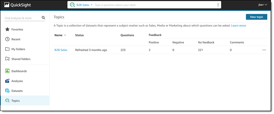
To recap, Q is a natural language query tool for the Enterprise Edition of QuickSight. Powered by machine learning, it makes your existing data more accessible, and therefore more valuable. Think of Q as your personal Business Intelligence Engineer or Data Analyst, one that is on call 24 hours a day and always ready to provide you with quick, meaningful results! You get high-quality results in seconds, always shown in an appropriate form.

Behind the scenes, Q uses Natural Language Understanding (NLU) to discover the intent of your question. Aided by models that have been trained to recognize vocabulary and concepts drawn from multiple domains (sales, marketing, retail, HR, advertising, financial services, health care, and so forth), Q is able to answer questions that refer all data sources supported by QuickSight. This includes data from AWS sources such as Amazon Redshift, Amazon Relational Database Service (RDS), Amazon Aurora, Amazon Athena, and Amazon Simple Storage Service (Amazon S3) as well as third party sources & SaaS apps such as Salesforce, Adobe Analytics, ServiceNow, and Excel.

Q in Action
Q is powered by topics, which are generally created by QuickSight Authors for use within an organization (if you are a QuickSight Author, you can learn more about getting started). Topics represent subject areas for questions, and are created interactively. To learn more about the five-step process that Authors use to create a topic, be sure to watch our new video, Tips to Create a Great Q Topic.

To use Q, I simply select a topic (B2B Sales in this case) and enter a question in the Q bar at the top of the page:

Q query --

In addition to the actual results, Q gives me access to explanatory information that I can review to ensure that my question was understood and processed as desired. For example, I can click on sales and learn how Q handles the field:

Detailed information on the use of the sales field.

I can fine-tune each aspect as well; here I clicked Sorted by:

Changing sort order for sales field.

Q chooses an appropriate visual representation for each answer, but I can fine-tune that as well:

Select a new visual type.

Perhaps I want a donut chart instead:

Now that you have seen how Q processes a question and gives you control over how the question is processed & displayed, let’s take a look at a few more questions, starting with “which product sells best in south?”

Question:

Here’s “what is total sales by region and category?” using the vertical stacked bar chart visual:

Total sales by region and catergory.

Behind the Scenes – Q Topics
As I mentioned earlier, Q uses topics to represent a particular subject matter. I click Topics to see the list of topics that I have created or that have been shared with me:

I click B2B Sales to learn more. The Summary page is designed to provide QuickSight Authors with information that they can use to fine-tune the topic:

Info about the B2B Sales Topic.

I can click on the Data tab and learn more about the list of fields that Q uses to answer questions. Each field can have some synonyms or friendly names to make the process of asking questions simpler and more natural:

List of fields for the B2B Sales topic.

I can expand a field (row) to learn more about how Q “understands” and uses the field. I can make changes in order to exercise control over the types of aggregations that make sense for the field, and I can also provide additional semantic information:

Information about the Product Name field.

As an example of providing additional semantic information, if the field’s Semantic Type is Location, I can choose the appropriate sub-type:

The User Activity tab shows me the questions that users are asking of this topic:

User activirty for the B2B Sales topic.

QuickSight Authors can use this tab to monitor user feedback, get a sense of the most common questions, and also use the common questions to drive improvements to the content provided on QuickSight dashboards.

Finally, the Verified answers tab shows the answers that have been manually reviewed and approved:

Things to Know
Here are a couple of things to know about Amazon QuickSight Q:

Pricing – There’s a monthly fee for each Reader and each Author; take a look at the QuickSight Pricing Page for more information.

Regions – Q is available in the US East (N. Virginia), US West (Oregon), US East (Ohio), Europe (Ireland), Europe (Frankfurt), and Europe (London) Regions.

Supported Languages – We are launching with question support in English.

Jeff;

AWS Cloud Builders – Career Transformation & Personal Growth

Post Syndicated from Jeff Barr original https://aws.amazon.com/blogs/aws/aws-cloud-builders-career-transformation-personal-growth/

Long-time readers of this blog know that I firmly believe in the power of education to improve lives. AWS Training and Certification equips people and organizations around the world with cloud computing education to build and validate cloud computing skills. With demand for cloud skills and experience at an all-time high, there’s never been a better time to get started.

On the training side you have a multitude of options for classroom and digital training, including offerings from AWS Training Partners. After you have been trained and have gained some experience, you can prepare for, schedule, and earn one or more of the eleven AWS Certifications.

I encourage you to spend some time watching our new AWS Cloud Builder Career Stories videos. In these videos you will hear some AWS Training and Certification success stories:

  • Uri Parush became a Serverless Architect and rode a wave of innovation.
  • David Webster became an AWS Technical Practice Lead after dreaming of becoming an inventor.
  • Karolina Boboli retrained as a Cloud Architect after a career as an accountant.
  • Florian Clanet reminisces about putting his first application into service and how it reminded him of designing lighting for a high school play.
  • Veliswa Boya trained for her AWS Certification and became the first female AWS Developer Advocate in Africa.
  • Karen Tovmasyan wrote his first book about cloud and remembered his first boxing match.
  • Sara Alasfoor built her first AWS data analytics solution and learned that she could tackle any obstacle.
  • Bruno Amaro Almedia was happy to be thanked for publishing his first article about AWS after earning twelve AWS certifications.
  • Nicola Racco was terrified and exhilarated when he released his first serverless project.

I hope that you enjoy the stories, and that they inspire you to embark on a learning journey of your own!

Jeff;

New for AWS Distro for OpenTelemetry – Tracing Support is Now Generally Available

Post Syndicated from Danilo Poccia original https://aws.amazon.com/blogs/aws/new-for-aws-distro-for-opentelemetry-tracing-support-is-now-generally-available/

Last year before re:Invent, we introduced the public preview of AWS Distro for OpenTelemetry, a secure distribution of the OpenTelemetry project supported by AWS. OpenTelemetry provides tools, APIs, and SDKs to instrument, generate, collect, and export telemetry data to better understand the behavior and the performance of your applications. Yesterday, upstream OpenTelemetry announced tracing stability milestone for its components. Today, I am happy to share that support for traces is now generally available in AWS Distro for OpenTelemetry.

Using OpenTelemetry, you can instrument your applications just once and then send traces to multiple monitoring solutions.

You can use AWS Distro for OpenTelemetry to instrument your applications running on Amazon Elastic Compute Cloud (Amazon EC2), Amazon Elastic Container Service (Amazon ECS), Amazon Elastic Kubernetes Service (EKS), and AWS Lambda, as well as on premises. Containers running on AWS Fargate and orchestrated via either ECS or EKS are also supported.

You can send tracing data collected by AWS Distro for OpenTelemetry to AWS X-Ray, as well as partner destinations such as:

You can use auto-instrumentation agents to collect traces without changing your code. Auto-instrumentation is available today for Java and Python applications. Auto-instrumentation support for Python currently only covers the AWS SDK. You can instrument your applications using other programming languages (such as Go, Node.js, and .NET) with the OpenTelemetry SDKs.

Let’s see how this works in practice for a Java application.

Visualizing Traces for a Java Application Using Auto-Instrumentation
I create a simple Java application that shows the list of my Amazon Simple Storage Service (Amazon S3) buckets and my Amazon DynamoDB tables:

package com.example.myapp;

import software.amazon.awssdk.regions.Region;
import software.amazon.awssdk.services.s3.S3Client;
import software.amazon.awssdk.services.s3.model.*;
import software.amazon.awssdk.services.dynamodb.model.DynamoDbException;
import software.amazon.awssdk.services.dynamodb.model.ListTablesResponse;
import software.amazon.awssdk.services.dynamodb.model.ListTablesRequest;
import software.amazon.awssdk.services.dynamodb.DynamoDbClient;

import java.util.List;

/**
 * Hello world!
 *
 */
public class App {

    public static void listAllTables(DynamoDbClient ddb) {

        System.out.println("DynamoDB Tables:");

        boolean moreTables = true;
        String lastName = null;

        while (moreTables) {
            try {
                ListTablesResponse response = null;
                if (lastName == null) {
                    ListTablesRequest request = ListTablesRequest.builder().build();
                    response = ddb.listTables(request);
                } else {
                    ListTablesRequest request = ListTablesRequest.builder().exclusiveStartTableName(lastName).build();
                    response = ddb.listTables(request);
                }

                List<String> tableNames = response.tableNames();

                if (tableNames.size() > 0) {
                    for (String curName : tableNames) {
                        System.out.format("* %s\n", curName);
                    }
                } else {
                    System.out.println("No tables found!");
                    System.exit(0);
                }

                lastName = response.lastEvaluatedTableName();
                if (lastName == null) {
                    moreTables = false;
                }
            } catch (DynamoDbException e) {
                System.err.println(e.getMessage());
                System.exit(1);
            }
        }

        System.out.println("Done!\n");
    }

    public static void listAllBuckets(S3Client s3) {

        System.out.println("S3 Buckets:");

        ListBucketsRequest listBucketsRequest = ListBucketsRequest.builder().build();
        ListBucketsResponse listBucketsResponse = s3.listBuckets(listBucketsRequest);
        listBucketsResponse.buckets().stream().forEach(x -> System.out.format("* %s\n", x.name()));

        System.out.println("Done!\n");
    }

    public static void listAllBucketsAndTables(S3Client s3, DynamoDbClient ddb) {
        listAllBuckets(s3);
        listAllTables(ddb);
    }

    public static void main(String[] args) {

        Region region = Region.EU_WEST_1;

        S3Client s3 = S3Client.builder().region(region).build();
        DynamoDbClient ddb = DynamoDbClient.builder().region(region).build();

        listAllBucketsAndTables(s3, ddb);

        s3.close();
        ddb.close();
    }
}

I package the application using Apache Maven. Here’s the Project Object Model (POM) file managing dependencies such as the AWS SDK for Java 2.x that I use to interact with S3 and DynamoDB:

<project xmlns="http://maven.apache.org/POM/4.0.0" xmlns:xsi="http://www.w3.org/2001/XMLSchema-instance" xsi:schemaLocation="http://maven.apache.org/POM/4.0.0 http://maven.apache.org/maven-v4_0_0.xsd">
  <modelVersion>4.0.0</modelVersion>
  <properties>
    <project.build.sourceEncoding>UTF-8</project.build.sourceEncoding>
  </properties>
  <groupId>com.example.myapp</groupId>
  <artifactId>myapp</artifactId>
  <packaging>jar</packaging>
  <version>1.0-SNAPSHOT</version>
  <name>myapp</name>
  <dependencyManagement>
    <dependencies>
      <dependency>
        <groupId>software.amazon.awssdk</groupId>
        <artifactId>bom</artifactId>
        <version>2.17.38</version>
        <type>pom</type>
        <scope>import</scope>
      </dependency>
    </dependencies>
  </dependencyManagement>
  <dependencies>
    <dependency>
      <groupId>junit</groupId>
      <artifactId>junit</artifactId>
      <version>3.8.1</version>
      <scope>test</scope>
    </dependency>
    <dependency>
      <groupId>software.amazon.awssdk</groupId>
      <artifactId>s3</artifactId>
    </dependency>
    <dependency>
      <groupId>software.amazon.awssdk</groupId>
      <artifactId>dynamodb</artifactId>
    </dependency>
  </dependencies>
  <build>
    <plugins>
      <plugin>
        <groupId>org.apache.maven.plugins</groupId>
        <artifactId>maven-compiler-plugin</artifactId>
        <version>3.8.1</version>
        <configuration>
          <source>8</source>
          <target>8</target>
        </configuration>
      </plugin>
      <plugin>
        <artifactId>maven-assembly-plugin</artifactId>
        <configuration>
          <archive>
            <manifest>
              <mainClass>com.example.myapp.App</mainClass>
            </manifest>
          </archive>
          <descriptorRefs>
            <descriptorRef>jar-with-dependencies</descriptorRef>
          </descriptorRefs>
        </configuration>
      </plugin>
    </plugins>
  </build>
</project>

I use Maven to create an executable Java Archive (JAR) file that includes all dependencies:

$ mvn clean compile assembly:single

To run the application and get tracing data, I need two components:

In one terminal, I run the AWS Distro for OpenTelemetry Collector using Docker:

$ docker run --rm -p 4317:4317 -p 55680:55680 -p 8889:8888 \
         -e AWS_REGION=eu-west-1 \
         -e AWS_PROFILE=default \
         -v ~/.aws:/root/.aws \
         --name awscollector public.ecr.aws/aws-observability/aws-otel-collector:latest

The collector is now ready to receive traces and forward them to a monitoring platform. By default, the AWS Distro for OpenTelemetry Collector sends traces to AWS X-Ray. I can change the exporter or add more exporters by editing the collector configuration. For example, I can follow the documentation to configure OLTP exporters to send telemetry data using the OLTP protocol. In the documentation, I also find how to configure other partner destinations. [[ It would be great it we had a link for the partner section, I can find only links to a specific partner ]]

I download the latest version of the AWS Distro for OpenTelemetry Auto-Instrumentation Java Agent. Now, I run my application and use the agent to capture telemetry data without having to add any specific instrumentation the code. In the OTEL_RESOURCE_ATTRIBUTES environment variable I set a name and a namespace for the service: [[ Are service.name and service.namespace being used by X-Ray? I couldn’t find them in the service map ]]

$ OTEL_RESOURCE_ATTRIBUTES=service.name=MyApp,service.namespace=MyTeam \
  java -javaagent:otel/aws-opentelemetry-agent.jar \
       -jar myapp/target/myapp-1.0-SNAPSHOT-jar-with-dependencies.jar

As expected, I get the list of my S3 buckets globally and of the DynamoDB tables in the Region.

To generate more tracing data, I run the previous command a few times. Each time I run the application, telemetry data is collected by the agent and sent to the collector. The collector buffers the data and then sends it to the configured exporters. By default, it is sending traces to X-Ray.

Now, I look at the service map in the AWS X-Ray console to see my application’s interactions with other services:

Console screenshot.

And there they are! Without any change in the code, I see my application’s calls to the S3 and DynamoDB APIs. There were no errors, and all the circles are green. Inside the circles, I find the average latency of the invocations and the number of transactions per minute.

Adding Spans to a Java Application
The information automatically collected can be improved by providing more information with the traces. For example, I might have interactions with the same service in different parts of my application, and it would be useful to separate those interactions in the service map. In this way, if there is an error or high latency, I would know which part of my application is affected.

One way to do so is to use spans or segments. A span represents a group of logically related activities. For example, the listAllBucketsAndTables method is performing two operations, one with S3 and one with DynamoDB. I’d like to group them together in a span. The quickest way with OpenTelemetry is to add the @WithSpan annotation to the method. Because the result of a method usually depends on its arguments, I also use the @SpanAttribute annotation to describe which arguments in the method invocation should be automatically added as attributes to the span.

@WithSpan
    public static void listAllBucketsAndTables(@SpanAttribute("title") String title, S3Client s3, DynamoDbClient ddb) {

        System.out.println(title);

        listAllBuckets(s3);
        listAllTables(ddb);
    }

To be able to use the @WithSpan and @SpanAttribute annotations, I need to import them into the code and add the necessary OpenTelemetry dependencies to the POM. All these changes are based on the OpenTelemetry specifications and don’t depend on the actual implementation that I am using, or on the tool that I will use to visualize or analyze the telemetry data. I have only to make these changes once to instrument my application. Isn’t that great?

To better see how spans work, I create another method that is running the same operations in reverse order, first listing the DynamoDB tables, then the S3 buckets:

    @WithSpan
    public static void listTablesFirstAndThenBuckets(@SpanAttribute("title") String title, S3Client s3, DynamoDbClient ddb) {

        System.out.println(title);

        listAllTables(ddb);
        listAllBuckets(s3);
    }

The application is now running the two methods (listAllBucketsAndTables and listTablesFirstAndThenBuckets) one after the other. For simplicity, here’s the full code of the instrumented application:

package com.example.myapp;

import software.amazon.awssdk.regions.Region;
import software.amazon.awssdk.services.s3.S3Client;
import software.amazon.awssdk.services.s3.model.*;
import software.amazon.awssdk.services.dynamodb.model.DynamoDbException;
import software.amazon.awssdk.services.dynamodb.model.ListTablesResponse;
import software.amazon.awssdk.services.dynamodb.model.ListTablesRequest;
import software.amazon.awssdk.services.dynamodb.DynamoDbClient;

import java.util.List;

import io.opentelemetry.extension.annotations.SpanAttribute;
import io.opentelemetry.extension.annotations.WithSpan;

/**
 * Hello world!
 *
 */
public class App {

    public static void listAllTables(DynamoDbClient ddb) {

        System.out.println("DynamoDB Tables:");

        boolean moreTables = true;
        String lastName = null;

        while (moreTables) {
            try {
                ListTablesResponse response = null;
                if (lastName == null) {
                    ListTablesRequest request = ListTablesRequest.builder().build();
                    response = ddb.listTables(request);
                } else {
                    ListTablesRequest request = ListTablesRequest.builder().exclusiveStartTableName(lastName).build();
                    response = ddb.listTables(request);
                }

                List<String> tableNames = response.tableNames();

                if (tableNames.size() > 0) {
                    for (String curName : tableNames) {
                        System.out.format("* %s\n", curName);
                    }
                } else {
                    System.out.println("No tables found!");
                    System.exit(0);
                }

                lastName = response.lastEvaluatedTableName();
                if (lastName == null) {
                    moreTables = false;
                }
            } catch (DynamoDbException e) {
                System.err.println(e.getMessage());
                System.exit(1);
            }
        }

        System.out.println("Done!\n");
    }

    public static void listAllBuckets(S3Client s3) {

        System.out.println("S3 Buckets:");

        ListBucketsRequest listBucketsRequest = ListBucketsRequest.builder().build();
        ListBucketsResponse listBucketsResponse = s3.listBuckets(listBucketsRequest);
        listBucketsResponse.buckets().stream().forEach(x -> System.out.format("* %s\n", x.name()));

        System.out.println("Done!\n");
    }

    @WithSpan
    public static void listAllBucketsAndTables(@SpanAttribute("title") String title, S3Client s3, DynamoDbClient ddb) {

        System.out.println(title);

        listAllBuckets(s3);
        listAllTables(ddb);

    }

    @WithSpan
    public static void listTablesFirstAndThenBuckets(@SpanAttribute("title") String title, S3Client s3, DynamoDbClient ddb) {

        System.out.println(title);

        listAllTables(ddb);
        listAllBuckets(s3);

    }

    public static void main(String[] args) {

        Region region = Region.EU_WEST_1;

        S3Client s3 = S3Client.builder().region(region).build();
        DynamoDbClient ddb = DynamoDbClient.builder().region(region).build();

        listAllBucketsAndTables("My S3 buckets and DynamoDB tables", s3, ddb);
        listTablesFirstAndThenBuckets("My DynamoDB tables first and then S3 bucket", s3, ddb);

        s3.close();
        ddb.close();
    }
}

And here’s the updated POM that includes the additional OpenTelemetry dependencies:

<project xmlns="http://maven.apache.org/POM/4.0.0" xmlns:xsi="http://www.w3.org/2001/XMLSchema-instance" xsi:schemaLocation="http://maven.apache.org/POM/4.0.0 http://maven.apache.org/maven-v4_0_0.xsd">
  <modelVersion>4.0.0</modelVersion>
  <properties>
    <project.build.sourceEncoding>UTF-8</project.build.sourceEncoding>
  </properties>
  <groupId>com.example.myapp</groupId>
  <artifactId>myapp</artifactId>
  <packaging>jar</packaging>
  <version>1.0-SNAPSHOT</version>
  <name>myapp</name>
  <dependencyManagement>
    <dependencies>
      <dependency>
        <groupId>software.amazon.awssdk</groupId>
        <artifactId>bom</artifactId>
        <version>2.16.60</version>
        <type>pom</type>
        <scope>import</scope>
      </dependency>
    </dependencies>
  </dependencyManagement>
  <dependencies>
    <dependency>
      <groupId>junit</groupId>
      <artifactId>junit</artifactId>
      <version>3.8.1</version>
      <scope>test</scope>
    </dependency>
    <dependency>
      <groupId>software.amazon.awssdk</groupId>
      <artifactId>s3</artifactId>
    </dependency>
    <dependency>
      <groupId>software.amazon.awssdk</groupId>
      <artifactId>dynamodb</artifactId>
    </dependency>
    <dependency>
      <groupId>io.opentelemetry</groupId>
      <artifactId>opentelemetry-extension-annotations</artifactId>
      <version>1.5.0</version>
    </dependency>
    <dependency>
      <groupId>io.opentelemetry</groupId>
      <artifactId>opentelemetry-api</artifactId>
      <version>1.5.0</version>
    </dependency>
  </dependencies>
  <build>
    <plugins>
      <plugin>
        <groupId>org.apache.maven.plugins</groupId>
        <artifactId>maven-compiler-plugin</artifactId>
        <version>3.8.1</version>
        <configuration>
          <source>8</source>
          <target>8</target>
        </configuration>
      </plugin>
      <plugin>
        <artifactId>maven-assembly-plugin</artifactId>
        <configuration>
          <archive>
            <manifest>
              <mainClass>com.example.myapp.App</mainClass>
            </manifest>
          </archive>
          <descriptorRefs>
            <descriptorRef>jar-with-dependencies</descriptorRef>
          </descriptorRefs>
        </configuration>
      </plugin>
    </plugins>
  </build>
</project>

I compile my application with these changes and run it again a few times:

$ mvn clean compile assembly:single

$ OTEL_RESOURCE_ATTRIBUTES=service.name=MyApp,service.namespace=MyTeam \
  java -javaagent:otel/aws-opentelemetry-agent.jar \
       -jar myapp/target/myapp-1.0-SNAPSHOT-jar-with-dependencies.jar

Now, let’s look at the X-Ray service map, computed using the additional information provided by those annotations.

Console screenshot.

Now I see the two methods and the other services they invoke. If there are errors or high latency, I can easily understand how the two methods are affected.

In the Traces section of the X-Ray console, I look at the Raw data for some of the traces. Because the title argument was annotated with @SpanAttribute, each trace has the value of that argument in the metadata section.

Console screenshot.

Collecting Traces from Lambda Functions
The previous steps work on premises, on EC2, and with applications running in containers. To collect traces and use auto-instrumentation with Lambda functions, you can use the AWS managed OpenTelemetry Lambda Layers (a few examples are included in the repository).

After you add the Lambda layer to your function, you can use the environment variable OPENTELEMETRY_COLLECTOR_CONFIG_FILE to pass your own configuration to the collector. More information on using AWS Distro for OpenTelemetry with AWS Lambda is available in the documentation.

Availability and Pricing
You can use AWS Distro for OpenTelemetry to get telemetry data from your application running on premises and on AWS. There are no additional costs for using AWS Distro for OpenTelemetry. Depending on your configuration, you might pay for the AWS services that are destinations for OpenTelemetry data, such as AWS X-Ray, Amazon CloudWatch, and Amazon Managed Service for Prometheus (AMP).

To learn more, you are invited to this webinar on Thursday, October 7 at 10:00 am PT / 1:00 pm EDT / 7:00 pm CEST.

Simplify the instrumentation of your applications and improve their observability using AWS Distro for OpenTelemetry today.

Danilo

In the Works – AWS Region in New Zealand

Post Syndicated from Jeff Barr original https://aws.amazon.com/blogs/aws/in-the-works-aws-region-in-new-zealand/

We are currently working on regions in Australia, India, Indonesia, Israel, Spain , Switzerland, and the United Arab Emirates.

Auckland, New Zealand in the Works
Today I am happy to announce that the new AWS Asia Pacific (Auckland) Region is in the works and will open in 2024. This region will have three Availability Zones and will give AWS customers in New Zealand the ability to run workloads and store data that must remain in-country.

There are 81 Availability Zones within 25 AWS Regions in operation today, with 24 more Availability Zones and eight announced regions (including this one) underway.

Each of the Availability Zones will be physically independent of the others in region, close enough to support applications that need low latency, yet sufficiently distant to significantly reduce the risk that an AZ-level event will have an impact on business continuity. The AZs in this region will be connected together via high-bandwidth, low-latency network connections over dedicated, fully redundant fiber. This connectivity supports applications that need synchronous replication between AZs for availability or redundancy; you can take a peek at the AWS Global Infrastructure page to learn more about how we design and build regions and AZs.

AWS in New Zealand
According to an economic impact study (EIS) that we released as part of this launch, we estimate that our NZ$ 7.5 billion (5.3 billion USD) investment will create 1,000 new jobs and will have an estimated economic impact of NZ$ 10.8 billion (7.7 billion USD) over the next fifteen years.

The first AWS office in New Zealand opened in 2013 and now employs over 100 solution architects, account managers, sales representatives, professional services consultants, and cloud experts.

Other AWS infrastructure includes a pair of Amazon CloudFront edge locations in Auckland along with access to the AWS global backbone through multiple, redundant submarine cables. For more information about connectivity options, be sure to check out New Zealand Internet Connectivity to AWS.

Stay Tuned
We’ll announce the opening of this and the other regions in future blog posts, so be sure to stay tuned!

Jeff;

PS – The Amazon Polly Aria voice (New Zealand English) was launched earlier this year and should be of interest to New Zealanders. Visit the Amazon Polly Console to get started!

Introducing Amazon MSK Connect – Stream Data to and from Your Apache Kafka Clusters Using Managed Connectors

Post Syndicated from Danilo Poccia original https://aws.amazon.com/blogs/aws/introducing-amazon-msk-connect-stream-data-to-and-from-your-apache-kafka-clusters-using-managed-connectors/

Apache Kafka is an open-source platform for building real-time streaming data pipelines and applications. At re:Invent 2018, we announced Amazon Managed Streaming for Apache Kafka, a fully managed service that makes it easy to build and run applications that use Apache Kafka to process streaming data.

When you use Apache Kafka, you capture real-time data from sources such as IoT devices, database change events, and website clickstreams, and deliver it to destinations such as databases and persistent storage.

Kafka Connect is an open-source component of Apache Kafka that provides a framework for connecting with external systems such as databases, key-value stores, search indexes, and file systems. However, manually running Kafka Connect clusters requires you to plan and provision the required infrastructure, deal with cluster operations, and scale it in response to load changes.

Today, we’re announcing a new capability that makes it easier to manage Kafka Connect clusters. MSK Connect allows you to configure and deploy a connector using Kafka Connect with a just few clicks. MSK Connect provisions the required resources and sets up the cluster. It continuously monitors the health and delivery state of connectors, patches and manages the underlying hardware, and auto-scales connectors to match changes in throughput. As a result, you can focus your resources on building applications rather than managing infrastructure.

MSK Connect is fully compatible with Kafka Connect, which means you can migrate your existing connectors without code changes. You don’t need an MSK cluster to use MSK Connect. It supports Amazon MSK, Apache Kafka, and Apache Kafka compatible clusters as sources and sinks. These clusters can be self-managed or managed by AWS partners and 3rd parties as long as MSK Connect can privately connect to the clusters.

Using MSK Connect with Amazon Aurora and Debezium
To test MSK Connect, I want to use it to stream data change events from one of my databases. To do so, I use Debezium, an open-source distributed platform for change data capture built on top of Apache Kafka.

I use a MySQL-compatible Amazon Aurora database as the source and the Debezium MySQL connector with the setup described in this architectural diagram:

Architectural diagram.

To use my Aurora database with Debezium, I need to turn on binary logging in the DB cluster parameter group. I follow the steps in the How do I turn on binary logging for my Amazon Aurora MySQL cluster article.

Next, I have to create a custom plugin for MSK Connect. A custom plugin is a set of JAR files that contain the implementation of one or more connectors, transforms, or converters. Amazon MSK will install the plugin on the workers of the connect cluster where the connector is running.

From the Debezium website, I download the MySQL connector plugin for the latest stable release. Because MSK Connect accepts custom plugins in ZIP or JAR format, I convert the downloaded archive to ZIP format and keep the JARs files in the main directory:

$ tar xzf debezium-connector-mysql-1.6.1.Final-plugin.tar.gz
$ cd debezium-connector-mysql
$ zip -9 ../debezium-connector-mysql-1.6.1.zip *
$ cd ..

Then, I use the AWS Command Line Interface (CLI) to upload the custom plugin to an Amazon Simple Storage Service (Amazon S3) bucket in the same AWS Region I am using for MSK Connect:

$ aws s3 cp debezium-connector-mysql-1.6.1.zip s3://my-bucket/path/

On the Amazon MSK console there is a new MSK Connect section. I look at the connectors and choose Create connector. Then, I create a custom plugin and browse my S3 buckets to select the custom plugin ZIP file I uploaded before.

Console screenshot.

I enter a name and a description for the plugin and then choose Next.

Console screenshot.

Now that the configuration of the custom plugin is complete, I start the creation of the connector. I enter a name and a description for the connector.

Console screenshot.

I have the option to use a self-managed Apache Kafka cluster or one that is managed by MSK. I select one of my MSK cluster that is configured to use IAM authentication. The MSK cluster I select is in the same virtual private cloud (VPC) as my Aurora database. To connect, the MSK cluster and Aurora database use the default security group for the VPC. For simplicity, I use a cluster configuration with auto.create.topics.enable set to true.

Console screenshot.

In Connector configuration, I use the following settings:

connector.class=io.debezium.connector.mysql.MySqlConnector
tasks.max=1
database.hostname=<aurora-database-writer-instance-endpoint>
database.port=3306
database.user=my-database-user
database.password=my-secret-password
database.server.id=123456
database.server.name=ecommerce-server
database.include.list=ecommerce
database.history.kafka.topic=dbhistory.ecommerce
database.history.kafka.bootstrap.servers=<bootstrap servers>
database.history.consumer.security.protocol=SASL_SSL
database.history.consumer.sasl.mechanism=AWS_MSK_IAM
database.history.consumer.sasl.jaas.config=software.amazon.msk.auth.iam.IAMLoginModule required;
database.history.consumer.sasl.client.callback.handler.class=software.amazon.msk.auth.iam.IAMClientCallbackHandler
database.history.producer.security.protocol=SASL_SSL
database.history.producer.sasl.mechanism=AWS_MSK_IAM
database.history.producer.sasl.jaas.config=software.amazon.msk.auth.iam.IAMLoginModule required;
database.history.producer.sasl.client.callback.handler.class=software.amazon.msk.auth.iam.IAMClientCallbackHandler
include.schema.changes=true

Some of these settings are generic and should be specified for any connector. For example:

  • connector.class is the Java class of the connector.
  • tasks.max is the maximum number of tasks that should be created for this connector.

Other settings are specific to the Debezium MySQL connector:

  • The database.hostname contains the writer instance endpoint of my Aurora database.
  • The database.server.name is a logical name of the database server. It is used for the names of the Kafka topics created by Debezium.
  • The database.include.list contains the list of databases hosted by the specified server.
  • The database.history.kafka.topic is a Kafka topic used internally by Debezium to track database schema changes.
  • The database.history.kafka.bootstrap.servers contains the bootstrap servers of the MSK cluster.
  • The final eight lines (database.history.consumer.* and database.history.producer.*) enable IAM authentication to access the database history topic.

In Connector capacity, I can choose between autoscaled or provisioned capacity. For this setup, I choose Autoscaled and leave all other settings at their defaults.

Console screenshot.

With autoscaled capacity, I can configure these parameters:

  • MSK Connect Unit (MCU) count per worker – Each MCU provides 1 vCPU of compute and 4 GB of memory.
  • The minimum and maximum number of workers.
  • Autoscaling utilization thresholds – The upper and lower target utilization thresholds on MCU consumption in percentage to trigger auto scaling.

Console screenshot.

There is a summary of the minimum and maximum MCUs, memory, and network bandwidth for the connector.

Console screenshot.

For Worker configuration, you can use the default one provided by Amazon MSK or provide your own configuration. In my setup, I use the default one.

In Access permissions, I create a IAM role. In the trusted entities, I add kafkaconnect.amazonaws.com to allow MSK Connect to assume the role.

The role is used by MSK Connect to interact with the MSK cluster and other AWS services. For my setup, I add:

The Debezium connector needs access to the cluster configuration to find the replication factor to use to create the history topic. For this reason, I add to the permissions policy the kafka-cluster:DescribeClusterDynamicConfiguration action (equivalent Apache Kafka’s DESCRIBE_CONFIGS cluster ACL).

Depending on your configuration, you might need to add more permissions to the role (for example, in case the connector needs access to other AWS resources such as an S3 bucket). If that is the case, you should add permissions before creating the connector.

In Security, the settings for authentication and encryption in transit are taken from the MSK cluster.

Console screenshot.

In Logs, I choose to deliver logs to CloudWatch Logs to have more information on the execution of the connector. By using CloudWatch Logs, I can easily manage retention and interactively search and analyze my log data with CloudWatch Logs Insights. I enter the log group ARN (it’s the same log group I used before in the IAM role) and then choose Next.

Console screenshot.

I review the settings and then choose Create connector. After a few minutes, the connector is running.

Testing MSK Connect with Amazon Aurora and Debezium
Now let’s test the architecture I just set up. I start an Amazon Elastic Compute Cloud (Amazon EC2) instance to update the database and start a couple of Kafka consumers to see Debezium in action. To be able to connect to both the MSK cluster and the Aurora database, I use the same VPC and assign the default security group. I also add another security group that gives me SSH access to the instance.

I download a binary distribution of Apache Kafka and extract the archive in the home directory:

$ tar xvf kafka_2.13-2.7.1.tgz

To use IAM to authenticate with the MSK cluster, I follow the instructions in the Amazon MSK Developer Guide to configure clients for IAM access control. I download the latest stable release of the Amazon MSK Library for IAM:

$ wget https://github.com/aws/aws-msk-iam-auth/releases/download/1.1.0/aws-msk-iam-auth-1.1.0-all.jar

In the ~/kafka_2.13-2.7.1/config/ directory I create a client-config.properties file to configure a Kafka client to use IAM authentication:

# Sets up TLS for encryption and SASL for authN.
security.protocol = SASL_SSL

# Identifies the SASL mechanism to use.
sasl.mechanism = AWS_MSK_IAM

# Binds SASL client implementation.
sasl.jaas.config = software.amazon.msk.auth.iam.IAMLoginModule required;

# Encapsulates constructing a SigV4 signature based on extracted credentials.
# The SASL client bound by "sasl.jaas.config" invokes this class.
sasl.client.callback.handler.class = software.amazon.msk.auth.iam.IAMClientCallbackHandler

I add a few lines to my Bash profile to:

  • Add Kafka binaries to the PATH.
  • Add the MSK Library for IAM to the CLASSPATH.
  • Create the BOOTSTRAP_SERVERS environment variable to store the bootstrap servers of my MSK cluster.
$ cat >> ~./bash_profile
export PATH=~/kafka_2.13-2.7.1/bin:$PATH
export CLASSPATH=/home/ec2-user/aws-msk-iam-auth-1.1.0-all.jar
export BOOTSTRAP_SERVERS=<bootstrap servers>

Then, I open three terminal connections to the instance.

In the first terminal connection, I start a Kafka consumer for a topic with the same name as the database server (ecommerce-server). This topic is used by Debezium to stream schema changes (for example, when a new table is created).

$ cd ~/kafka_2.13-2.7.1/
$ kafka-console-consumer.sh --bootstrap-server $BOOTSTRAP_SERVERS \
                            --consumer.config config/client-config.properties \
                            --topic ecommerce-server --from-beginning

In the second terminal connection, I start another Kafka consumer for a topic with a name built by concatenating the database server (ecommerce-server), the database (ecommerce), and the table (orders). This topic is used by Debezium to stream data changes for the table (for example, when a new record is inserted).

$ cd ~/kafka_2.13-2.7.1/
$ kafka-console-consumer.sh --bootstrap-server $BOOTSTRAP_SERVERS \
                            --consumer.config config/client-config.properties \
                            --topic ecommerce-server.ecommerce.orders --from-beginning

In the third terminal connection, I install a MySQL client using the MariaDB package and connect to the Aurora database:

$ sudo yum install mariadb
$ mysql -h <aurora-database-writer-instance-endpoint> -u <database-user> -p

From this connection, I create the ecommerce database and a table for my orders:

CREATE DATABASE ecommerce;

USE ecommerce

CREATE TABLE orders (
       order_id VARCHAR(255),
       customer_id VARCHAR(255),
       item_description VARCHAR(255),
       price DECIMAL(6,2),
       order_date DATETIME DEFAULT CURRENT_TIMESTAMP
);

These database changes are captured by the Debezium connector managed by MSK Connect and are streamed to the MSK cluster. In the first terminal, consuming the topic with schema changes, I see the information on the creation of database and table:

Struct{source=Struct{version=1.6.1.Final,connector=mysql,name=ecommerce-server,ts_ms=1629202831473,db=ecommerce,server_id=1980402433,file=mysql-bin-changelog.000003,pos=9828,row=0},databaseName=ecommerce,ddl=CREATE DATABASE ecommerce,tableChanges=[]}
Struct{source=Struct{version=1.6.1.Final,connector=mysql,name=ecommerce-server,ts_ms=1629202878811,db=ecommerce,table=orders,server_id=1980402433,file=mysql-bin-changelog.000003,pos=10002,row=0},databaseName=ecommerce,ddl=CREATE TABLE orders ( order_id VARCHAR(255), customer_id VARCHAR(255), item_description VARCHAR(255), price DECIMAL(6,2), order_date DATETIME DEFAULT CURRENT_TIMESTAMP ),tableChanges=[Struct{type=CREATE,id="ecommerce"."orders",table=Struct{defaultCharsetName=latin1,primaryKeyColumnNames=[],columns=[Struct{name=order_id,jdbcType=12,typeName=VARCHAR,typeExpression=VARCHAR,charsetName=latin1,length=255,position=1,optional=true,autoIncremented=false,generated=false}, Struct{name=customer_id,jdbcType=12,typeName=VARCHAR,typeExpression=VARCHAR,charsetName=latin1,length=255,position=2,optional=true,autoIncremented=false,generated=false}, Struct{name=item_description,jdbcType=12,typeName=VARCHAR,typeExpression=VARCHAR,charsetName=latin1,length=255,position=3,optional=true,autoIncremented=false,generated=false}, Struct{name=price,jdbcType=3,typeName=DECIMAL,typeExpression=DECIMAL,length=6,scale=2,position=4,optional=true,autoIncremented=false,generated=false}, Struct{name=order_date,jdbcType=93,typeName=DATETIME,typeExpression=DATETIME,position=5,optional=true,autoIncremented=false,generated=false}]}}]}

Then, I go back to the database connection in the third terminal to insert a few records in the orders table:

INSERT INTO orders VALUES ("123456", "123", "A super noisy mechanical keyboard", "50.00", "2021-08-16 10:11:12");
INSERT INTO orders VALUES ("123457", "123", "An extremely wide monitor", "500.00", "2021-08-16 11:12:13");
INSERT INTO orders VALUES ("123458", "123", "A too sensible microphone", "150.00", "2021-08-16 12:13:14");

In the second terminal, I see the information on the records inserted into the orders table:

Struct{after=Struct{order_id=123456,customer_id=123,item_description=A super noisy mechanical keyboard,price=50.00,order_date=1629108672000},source=Struct{version=1.6.1.Final,connector=mysql,name=ecommerce-server,ts_ms=1629202993000,db=ecommerce,table=orders,server_id=1980402433,file=mysql-bin-changelog.000003,pos=10464,row=0},op=c,ts_ms=1629202993614}
Struct{after=Struct{order_id=123457,customer_id=123,item_description=An extremely wide monitor,price=500.00,order_date=1629112333000},source=Struct{version=1.6.1.Final,connector=mysql,name=ecommerce-server,ts_ms=1629202993000,db=ecommerce,table=orders,server_id=1980402433,file=mysql-bin-changelog.000003,pos=10793,row=0},op=c,ts_ms=1629202993621}
Struct{after=Struct{order_id=123458,customer_id=123,item_description=A too sensible microphone,price=150.00,order_date=1629115994000},source=Struct{version=1.6.1.Final,connector=mysql,name=ecommerce-server,ts_ms=1629202993000,db=ecommerce,table=orders,server_id=1980402433,file=mysql-bin-changelog.000003,pos=11114,row=0},op=c,ts_ms=1629202993630}

My change data capture architecture is up and running and the connector is fully managed by MSK Connect.

Availability and Pricing
MSK Connect is available in the following AWS Regions: Asia Pacific (Mumbai), Asia Pacific (Seoul), Asia Pacific (Singapore), Asia Pacific (Sydney), Asia Pacific (Tokyo), Canada (Central), EU (Frankfurt), EU (Ireland), EU (London), EU (Paris), EU (Stockholm), South America (Sao Paulo), US East (N. Virginia), US East (Ohio), US West (N. California), US West (Oregon). For more information, see the AWS Regional Services List.

With MSK Connect you pay for what you use. The resources used by your connectors can be scaled automatically based on your workload. For more information, see the Amazon MSK pricing page.

Simplify the management of your Apache Kafka connectors today with MSK Connect.

Danilo

New – Amazon EC2 VT1 Instances for Live Multi-stream Video Transcoding

Post Syndicated from Channy Yun original https://aws.amazon.com/blogs/aws/new-amazon-ec2-vt1-instances-for-live-multi-stream-video-transcoding/

Global demand for video content has been rapidly increasing and now has the major audiences of Internet and mobile network traffic. Over-the-top streaming services such as Twitch continue to see an explosion of content creators who are seeking live delivery with great image quality, while live event broadcasters are increasingly looking to embrace agile cloud infrastructure to reduce costs without sacrificing reliability, and efficiently scale with demand.

Today, I am happy to announce the general availability of Amazon EC2 VT1 instances that are designed to provide the best price performance for multi-stream video transcoding with resolutions up to 4K UHD. These VT1 instances feature Xilinx® Alveo™ U30 media accelerator transcoding cards with accelerated H.264/AVC and H.265/HEVC codecs and provide up to 30% better price per stream compared to the latest GPU-based EC2 instances and up to 60% better price per stream compared to the latest CPU-based EC2 instances.

Customers with their own live broadcast and streaming video pipelines can use VT1 instances to transcode video streams with resolutions up to 4K UHD. VT1 instances feature networking interfaces of up to 25 Gbps that can ingest multiple video streams over IP with low latency and low jitter. This capability makes it possible for these customers to fully embrace scalable, cost-effective, and resilient infrastructure.

Amazon EC2 VT1 Instance Type
EC2 VT1 instances are available in three sizes. The accelerated H.264/AVC and H.265/HEVC codecs are integrated into Xilinx Zynq ZU7EV SoCs. Each Xilinx® Alveo™ U30 media transcoding accelerator card contains two Zynq SoCs.

Instance size vCPUs Xilinx U30 card Memory Network bandwidth EBS-optimized bandwidth 1080p60 Streams per instance
vt1.3xlarge 12 1 24GB Up to 25 Gbps Up to 4.75 Gbps 8
vt1.6xlarge 24 2 48GB 25 Gbps 4.75 Gbps 16
vt1.24xlarge 96 8 192GB 25 Gbps 19 Gbps 64

The VT1 instances are suitable for transcoding multiple streams per instance. The streams can be processed independently in parallel or mixed (picture-in-picture, side-by-side, transitions). The vCPU cores help with implementing image processing, audio processing, and multiplexing. The Xilinx® Alveo™ U30 card can simultaneously output multiple streams at different resolutions (1080p, 720p, 480p, and 360p) and in both H.264 and H.265.

Each VT1 instance can be configured to produce parallel encoding with different settings, resolutions and transmission bit rate (“ABR ladders“). For example, a 4K UHD stream can be encoded at 60 frames per second with H.265 for high resolution display. Multiple lower resolutions can be encoded with H.264 for delivery to standard displays.

Get Started with EC2 VT1 Instances
You can now launch VT1 instances in the Amazon EC2 console, AWS Command Line Interface (AWS CLI), or using an SDK with the Amazon EC2 API.

We provide a number of sample video processing pipelines for the VT1 instances. There are tutorials and code examples in the GitHub repository that cover how to tune the codecs for image quality and transcoding latency, call the runtime for the U30 cards directly from your own applications, incorporate video filters such as titling and watermarking, and deploy with container orchestration frameworks.

Xilinx provides the “Xilinx Video Transcoding SDK” which includes:

VT1 instances can be coupled with Amazon Elastic Container Service (Amazon ECS) and Amazon Elastic Kubernetes Service (Amazon EKS) to efficiently scale transcoding workloads and with Amazon CloudFront to deliver content globally. VT1 instances can also be launched with Amazon Machine Images (AMIs) and containers developed by AWS Marketplace partners, such as Nginx for supplemental video processing functionality.

You can complement VT1 instances with AWS Media Services for reliable packaging and origination of transcoded content. To learn more, you can use a solution library of Live Streaming on AWS to build a live video workflow using these AWS services.

Available Now
Amazon EC2 VT1 instances are now available in the US East (N. Virginia), US West (Oregon), Europe (Ireland), Asia Pacific (Tokyo) Regions. To learn more, visit the EC2 VT1 instance page. Please send feedback to the AWS forum for Amazon EC2 or through your usual AWS support contacts.

– Channy