Post Syndicated from turnoff.us original http://turnoff.us/geek/insecurity-system/

Post Syndicated from turnoff.us original http://turnoff.us/geek/insecurity-system/
Post Syndicated from Let's Encrypt original https://letsencrypt.org/2024/03/19/new-intermediate-certificates/
On Wednesday, March 13, 2024, Let’s Encrypt generated 10 new Intermediate CA Key Pairs, and issued 15 new Intermediate CA Certificates containing the new public keys. These new intermediate certificates provide smaller and more efficient certificate chains to Let’s Encrypt Subscribers, enhancing the overall online experience in terms of speed, security, and accessibility.
First, a bit of history. In September, 2020, Let’s Encrypt issued a new root and collection of intermediate certificates. Those certificates helped us improve the privacy and efficiency of Web security by making ECDSA end-entity certificates widely available. However, those intermediates are approaching their expiration dates, so it is time to replace them.
Our new batch of intermediates are very similar to the ones we issued in 2020, with a few small changes. We’re going to go over what those changes are and why we made them.
We created 5 new 2048-bit RSA intermediate certificates named in sequence from R10 through R14. These are issued by ISRG Root X1. You can think of them as direct replacements for our existing R3 and R4 intermediates.
We also created 5 new P-384 ECDSA intermediate certificates named in sequence from E5 through E9. Each of these is represented by two certificates: one issued by ISRG Root X2 (exactly like our existing E1 and E2), and one issued (or cross-signed) by ISRG Root X1.
You can see details of all of the certificates on our updated hierarchy page.
Rotating the set of intermediates we issue from helps keep the Internet agile and more secure. It encourages automation and efficiency, and discourages outdated practices like key pinning. “Key Pinning” is a practice in which clients — either ACME clients getting certificates for their site, or apps connecting to their own backend servers — decide to trust only a single issuing intermediate certificate rather than delegating trust to the system trust store. Updating pinned keys is a manual process, which leads to an increased risk of errors and potential business continuity failures.
Intermediates usually change only every five years, so this joint is exercised infrequently and client software keeps making the same mistakes. Shortening the lifetime from five years to three years means we will be conducting another ceremony in just two years, ahead of the expiration date on these recently created certificates. This ensures we exercise the joint more frequently than in the past.
We also issued more intermediates this time around. Historically, we’ve had two of each key type (RSA and ECDSA): one for active issuance, and one held as a backup for emergencies. Moving forward we will have five: two conducting active issuance, two waiting in the wings to be introduced in about one year, and one for emergency backup. Randomizing the selected issuer for a given key type means it will be impossible to predict which intermediate a certificate will be issued from. We are very hopeful that these steps will prevent intermediate key pinning altogether, and help the WebPKI remain agile moving forward.
These shorter intermediate lifetimes and randomized intermediate issuance shouldn’t impact the online experience of the general Internet user. Subscribers may be impacted if they are pinning one of our intermediates, though this should be incredibly rare.
When we issued ISRG Root X2 in 2020, we decided to cross-sign it from ISRG Root X1 so that it would be trusted even by systems that didn’t yet have ISRG Root X2 in their trust store. This meant that Subscribers who wanted issuance from our ECDSA intermediates would have a choice: they could either have a very short, ECDSA-only, but low-compatibility chain terminating at ISRG Root X2, or they could have a longer, high-compatibility chain terminating at ISRG Root X1. At the time, this tradeoff (TLS handshake size vs compatibility) seemed like a reasonable choice to provide, and we provided the high-compatibility chain by default to support the largest number of configurations.
ISRG Root X2 is now trusted by most platforms, and we can now offer an improved version of the same choice. The same very short, ECDSA-only chain will still be available for Subscribers who want to optimize their TLS handshakes at the cost of some compatibility. But the high-compatibility chain will be drastically improving: instead of containing two intermediates (both E1 and the cross-signed ISRG Root X2), it will now contain only a single intermediate: the version of one of our new ECDSA intermediates cross-signed by ISRG Root X1.
This reduces the size of our default ECDSA chain by about a third, and is an important step towards removing our ECDSA allow-list.
We’ve made two other tiny changes that are worth mentioning, but will have no impact on how Subscribers and clients use our certificates:
We’ve changed how the Subject Key ID field is calculated, from a SHA-1 hash of the public key, to a truncated SHA-256 hash of the same data. Although this use of SHA-1 was not cryptographically relevant, it is still nice to remove one more usage of that broken algorithm, helping move towards a world where cryptography libraries don’t need to include SHA-1 support at all.
We have removed our CPS OID from the Certificate Policies extension. This saves a few bytes in the certificate, which can add up to a lot of bandwidth saved over the course of billions of TLS handshakes.
Both of these mirror two identical changes that we made for our Subscriber Certificates in the past year.
We intend to put two of each of the new RSA and ECDSA keys into rotation in the next few months. Two of each will be ready to swap in at a future date, and one of each will be held in reserve in case of an emergency. Read more about the strategy in our December 2023 post on the Community Forum.
Not familiar with the forum? It’s where Let’s Encrypt publishes updates on our Issuance Tech and APIs. It’s also where you can go for troubleshooting help from community experts and Let’s Encrypt staff. Check it out and subscribe to alerts for technical updates.
We hope that this has been an interesting and informative tour around our new intermediates, and we look forward to continuing to improve the Internet, one certificate at a time.
We depend on contributions from our community of users and supporters in order to provide our services. If your company or organization would like to sponsor Let’s Encrypt please email us at [email protected]. We ask that you make an individual contribution if it is within your means.
Post Syndicated from Let's Encrypt original https://letsencrypt.org/2024/03/19/new-intermediate-certificates.html
On Wednesday, March 13, 2024, Let’s Encrypt generated 10 new Intermediate CA Key Pairs, and issued 15 new Intermediate CA Certificates containing the new public keys. These new intermediate certificates provide smaller and more efficient certificate chains to Let’s Encrypt Subscribers, enhancing the overall online experience in terms of speed, security, and accessibility.
First, a bit of history. In September, 2020, Let’s Encrypt issued a new root and collection of intermediate certificates. Those certificates helped us improve the privacy and efficiency of Web security by making ECDSA end-entity certificates widely available. However, those intermediates are approaching their expiration dates, so it is time to replace them.
Our new batch of intermediates are very similar to the ones we issued in 2020, with a few small changes. We’re going to go over what those changes are and why we made them.
We created 5 new 2048-bit RSA intermediate certificates named in sequence from R10 through R14. These are issued by ISRG Root X1. You can think of them as direct replacements for our existing R3 and R4 intermediates.
We also created 5 new P-384 ECDSA intermediate certificates named in sequence from E5 through E9. Each of these is represented by two certificates: one issued by ISRG Root X2 (exactly like our existing E1 and E2), and one issued (or cross-signed) by ISRG Root X1.
You can see details of all of the certificates on our updated hierarchy page.
Rotating the set of intermediates we issue from helps keep the Internet agile and more secure. It encourages automation and efficiency, and discourages outdated practices like key pinning. “Key Pinning” is a practice in which clients — either ACME clients getting certificates for their site, or apps connecting to their own backend servers — decide to trust only a single issuing intermediate certificate rather than delegating trust to the system trust store. Updating pinned keys is a manual process, which leads to an increased risk of errors and potential business continuity failures.
Intermediates usually change only every five years, so this joint is exercised infrequently and client software keeps making the same mistakes. Shortening the lifetime from five years to three years means we will be conducting another ceremony in just two years, ahead of the expiration date on these recently created certificates. This ensures we exercise the joint more frequently than in the past.
We also issued more intermediates this time around. Historically, we’ve had two of each key type (RSA and ECDSA): one for active issuance, and one held as a backup for emergencies. Moving forward we will have five: two conducting active issuance, two waiting in the wings to be introduced in about one year, and one for emergency backup. Randomizing the selected issuer for a given key type means it will be impossible to predict which intermediate a certificate will be issued from. We are very hopeful that these steps will prevent intermediate key pinning altogether, and help the WebPKI remain agile moving forward.
These shorter intermediate lifetimes and randomized intermediate issuance shouldn’t impact the online experience of the general Internet user. Subscribers may be impacted if they are pinning one of our intermediates, though this should be incredibly rare.
When we issued ISRG Root X2 in 2020, we decided to cross-sign it from ISRG Root X1 so that it would be trusted even by systems that didn’t yet have ISRG Root X2 in their trust store. This meant that Subscribers who wanted issuance from our ECDSA intermediates would have a choice: they could either have a very short, ECDSA-only, but low-compatibility chain terminating at ISRG Root X2, or they could have a longer, high-compatibility chain terminating at ISRG Root X1. At the time, this tradeoff (TLS handshake size vs compatibility) seemed like a reasonable choice to provide, and we provided the high-compatibility chain by default to support the largest number of configurations.
ISRG Root X2 is now trusted by most platforms, and we can now offer an improved version of the same choice. The same very short, ECDSA-only chain will still be available for Subscribers who want to optimize their TLS handshakes at the cost of some compatibility. But the high-compatibility chain will be drastically improving: instead of containing two intermediates (both E1 and the cross-signed ISRG Root X2), it will now contain only a single intermediate: the version of one of our new ECDSA intermediates cross-signed by ISRG Root X1.
This reduces the size of our default ECDSA chain by about a third, and is an important step towards removing our ECDSA allow-list.
We’ve made two other tiny changes that are worth mentioning, but will have no impact on how Subscribers and clients use our certificates:
We’ve changed how the Subject Key ID field is calculated, from a SHA-1 hash of the public key, to a truncated SHA-256 hash of the same data. Although this use of SHA-1 was not cryptographically relevant, it is still nice to remove one more usage of that broken algorithm, helping move towards a world where cryptography libraries don’t need to include SHA-1 support at all.
We have removed our CPS OID from the Certificate Policies extension. This saves a few bytes in the certificate, which can add up to a lot of bandwidth saved over the course of billions of TLS handshakes.
Both of these mirror two identical changes that we made for our Subscriber Certificates in the past year.
We intend to put two of each of the new RSA and ECDSA keys into rotation in the next few months. Two of each will be ready to swap in at a future date, and one of each will be held in reserve in case of an emergency. Read more about the strategy in our December 2023 post on the Community Forum.
Not familiar with the forum? It’s where Let’s Encrypt publishes updates on our Issuance Tech and APIs. It’s also where you can go for troubleshooting help from community experts and Let’s Encrypt staff. Check it out and subscribe to alerts for technical updates.
We hope that this has been an interesting and informative tour around our new intermediates, and we look forward to continuing to improve the Internet, one certificate at a time.
We depend on contributions from our community of users and supporters in order to provide our services. If your company or organization would like to sponsor Let’s Encrypt please email us at [email protected]. We ask that you make an individual contribution if it is within your means.
Post Syndicated from Lorenzo Nicora original https://aws.amazon.com/blogs/big-data/amazon-managed-service-for-apache-flink-now-supports-apache-flink-version-1-18/
Apache Flink is an open source distributed processing engine, offering powerful programming interfaces for both stream and batch processing, with first-class support for stateful processing and event time semantics. Apache Flink supports multiple programming languages, Java, Python, Scala, SQL, and multiple APIs with different level of abstraction, which can be used interchangeably in the same application.
Amazon Managed Service for Apache Flink, which offers a fully managed, serverless experience in running Apache Flink applications, now supports Apache Flink 1.18.1, the latest version of Apache Flink at the time of writing.
In this post, we discuss some of the interesting new features and capabilities of Apache Flink, introduced with the most recent major releases, 1.16, 1.17, and 1.18, and now supported in Managed Service for Apache Flink.
Before we dive into the new functionalities of Apache Flink available with version 1.18.1, let’s explore the new capabilities that come from the availability of many new open source connectors.
A dedicated OpenSearch connector is now available to be included in your projects, enabling an Apache Flink application to write data directly into OpenSearch, without relying on Elasticsearch compatibility mode. This connector is compatible with Amazon OpenSearch Service provisioned and OpenSearch Service Serverless.
This new connector supports SQL and Table APIs, working with both Java and Python, and the DataStream API, for Java only. Out of the box, it provides at-least-once guarantees, synchronizing the writes with Flink checkpointing. You can achieve exactly-once semantics using deterministic IDs and upsert method.
By default, the connector uses OpenSearch version 1.x client libraries. You can switch to version 2.x by adding the correct dependencies.
Apache Flink developers can now use a dedicated connector to write data into Amazon DynamoDB. This connector is based on the Apache Flink AsyncSink, developed by AWS and now an integral part of the Apache Flink project, to simplify the implementation of efficient sink connectors, using non-blocking write requests and adaptive batching.
This connector also supports both SQL and Table APIs, Java and Python, and DataStream API, for Java only. By default, the sink writes in batches to optimize throughput. A notable feature of the SQL version is support for the PARTITIONED BY clause. By specifying one or more keys, you can achieve some client-side deduplication, only sending the latest record per key with each batch write. An equivalent can be achieved with the DataStream API by specifying a list of partition keys for overwriting within each batch.
This connector only works as a sink. You cannot use it for reading from DynamoDB. To look up data in DynamoDB, you still need to implement a lookup using the Flink Async I/O API or implementing a custom user-defined function (UDF), for SQL.
Another interesting connector is for MongoDB. In this case, both source and sink are available, for both the SQL and Table APIs and DataStream API. The new connector is now officially part of the Apache Flink project and supported by the community. This new connector replaces the old one provided by MongoDB directly, which only supports older Flink Sink and Source APIs.
As for other data store connectors, the source can either be used as a bounded source, in batch mode, or for lookups. The sink works both in batch mode and streaming, supporting both upsert and append mode.
Among the many notable features of this connector, one that’s worth mentioning is the ability to enable caching when using the source for lookups. Out of the box, the sink supports at-least-once guarantees. When a primary key is defined, the sink can support exactly-once semantics via idempotent upserts. The sink connector also supports exactly-once semantics, with idempotent upserts, when the primary key is defined.
Not a new feature, but an important factor to consider when updating an older Apache Flink application, is the new connector versioning. Starting from Apache Flink version 1.17, most connectors have been externalized from the main Apache Flink distribution and follow independent versioning.
To include the right dependency, you need to specify the artifact version with the form: <connector-version>-<flink-version>
For example, the latest Kafka connector, also working with Amazon Managed Streaming for Apache Kafka (Amazon MSK), at the time of writing is version 3.1.0. If you are using Apache Flink 1.18, the dependency to use will be the following:
For Amazon Kinesis, the new connector version is 4.2.0. The dependency for Apache Flink 1.18 will be the following:
In the following sections, we discuss more of the powerful new features now available in Apache Flink 1.18 and supported in Amazon Managed Service for Apache Flink.
In Apache Flink SQL, users can provide hints to join queries that can be used to suggest the optimizer to have an effect in the query plan. In particular, in streaming applications, lookup joins are used to enrich a table, representing streaming data, with data that is queried from an external system, typically a database. Since version 1.16, several improvements have been introduced for lookup joins, allowing you to adjust the behavior of the join and improve performance:
FULL, for a small dataset that can be held entirely in memory, PARTIAL, for a large dataset, only caching the most recent records, or NONE, to completely disable cache. For PARTIAL cache, you can also configure the number of rows to buffer and the time-to-live.PARTIAL or NONE lookup cache, to configure the behavior in case of a failed lookup in the external database.All these behaviors can be controlled using a LOOKUP hint, like in the following example, where we show a lookup join using async lookup:
In this section, we discuss new improvements and support in PyFlink.
Apache Flink newest versions introduced several improvements for PyFlink users. First and foremost, Python 3.10 is now supported, and Python 3.6 support has been completely removed (FLINK-29421). Managed Service for Apache Flink currently uses Python 3.10 runtime to run PyFlink applications.
From the perspective of the programming API, PyFlink is getting closer to Java on every version. The DataStream API now supports features like side outputs and broadcast state, and gaps on windowing API have been closed. PyFlink also now supports new connectors like Amazon Kinesis Data Streams directly from the DataStream API.
PyFlink is very efficient. The overhead of running Flink API operators in PyFlink is minimal compared to Java or Scala, because the runtime actually runs the operator implementation in the JVM directly, regardless of the language of your application. But when you have a user-defined function, things are slightly different. A line of Python code as simple as lambda x: x + 1, or as complex as a Pandas function, must run in a Python runtime.
By default, Apache Flink runs a Python runtime on each Task Manager, external to the JVM. Each record is serialized, handed to the Python runtime via inter-process communication, deserialized, and processed in the Python runtime. The result is then serialized and handed back to the JVM, where it’s deserialized. This is the PyFlink PROCESS mode. It’s very stable but it introduces an overhead, and in some cases, it may become a performance bottleneck.
Since version 1.15, Apache Flink also supports THREAD mode for PyFlink. In this mode, Python user-defined functions are run within the JVM itself, removing the serialization/deserialization and inter-process communication overhead. THREAD mode has some limitations; for example, THREAD mode cannot be used for Pandas or UDAFs (user-defined aggregate functions, consisting of many input records and one output record), but can substantially improve performance of a PyFlink application.
With version 1.16, the support of THREAD mode has been substantially extended, also covering the Python DataStream API.
THREAD mode is supported by Managed Service for Apache Flink, and can be enabled directly from your PyFlink application.
If you use Apple Silicon-based machines to develop PyFlink applications, developing for PyFlink 1.15, you have probably encountered some of the known Python dependency issues on Apple Silicon. These issues have been finally resolved (FLINK-25188). These limitations did not affect PyFlink applications running on Managed Service for Apache Flink. Before version 1.16, if you wanted to develop a PyFlink application on a machine using M1, M2, or M3 chipset, you had to use some workarounds, because it was impossible to install PyFlink 1.15 or earlier directly on the machine.
Apache Flink 1.15 already supported Incremental Checkpoints and Buffer Debloating. These features can be used, particularly in combination, to improve checkpoint performance, making checkpointing duration more predictable, especially in the presence of backpressure. For more information about these features, see Optimize checkpointing in your Amazon Managed Service for Apache Flink applications with buffer debloating and unaligned checkpoints.
With versions 1.16 and 1.17, several changes have been introduced to improve stability and performance.
Apache Flink uses watermarks to support event-time semantics. Watermarks are special records, normally injected in the flow from the source operator, that mark the progress of event time for operators like event time windowing aggregations. A common technique is delaying watermarks from the latest observed event time, to allow events to be out of order, at least to some degree.
However, the use of watermarks comes with a challenge. When the application has multiple sources, for example it receives events from multiple partitions of a Kafka topic, watermarks are generated independently for each partition. Internally, each operator always waits for the same watermark on all input partitions, practically aligning it on the slowest partition. The drawback is that if one of the partitions is not receiving data, watermarks don’t progress, increasing the end-to-end latency. For this reason, an optional idleness timeout has been introduced in many streaming sources. After the configured timeout, watermark generation ignores any partition not receiving any record, and watermarks can progress.
You can also face a similar but opposite challenge if one source is receiving events much faster than the others. Watermarks are aligned to the slowest partition, meaning that any windowing aggregation will wait for the watermark. Records from the fast source have to wait, being buffered. This may result in buffering an excessive volume of data, and an uncontrollable growth of operator state.
To address the issue of faster sources, starting with Apache Flink 1.17, you can enable watermark alignment of source splits (FLINK-28853). This mechanism, disabled by default, makes sure that no partitions progress their watermarks too fast, compared to other partitions. You can bind together multiple sources, like multiple input topics, assigning the same alignment group ID, and configuring the duration of the maximal drift from the current watermark. If one specific partition is receiving events too fast, the source operator pauses consuming that partition until the drift is reduced below the configured threshold.
You can enable it for each source separately. All you need is to specify an alignment group ID, which will bind together all sources that have the same ID, and the duration of the maximal drift from the current minimal watermark. This will pause consuming from the source subtask that are advancing too fast, until the drift is lower than the threshold specified.
The following code snippet shows how you can set up watermark alignment of source splits on a Kafka source emitting bounded-out-of-orderness watermarks:
This feature is only available with FLIP-217 compatible sources, supporting watermark alignment of source splits. As of writing, among major streaming source connectors, only Kafka source supports this feature.
The SQL and Table APIs now directly support Protobuf format. To use this format, you need to generate the Protobuf Java classes from the .proto schema definition files and include them as dependencies in your application.
The Protobuf format only works with the SQL and Table APIs and only to read or write Protobuf-serialized data from a source or to a sink. Currently, Flink doesn’t directly support Protobuf to serialize state directly and it doesn’t support schema evolution, as it does for Avro, for example. You still need to register a custom serializer with some overhead for your application.
Apache Flink internally relies on Akka for sending data between subtasks. In 2022, Lightbend, the company behind Akka, announced a license change for future Akka versions, from Apache 2.0 to a more restrictive license, and that Akka 2.6, the version used by Apache Flink, would not receive any further security update or fix.
Although Akka has been historically very stable and doesn’t require frequent updates, this license change represented a risk for the Apache Flink project. The decision of the Apache Flink community was to replace Akka with a fork of the version 2.6, called Apache Pekko (FLINK-32468). This fork will retain the Apache 2.0 license and receive any required updates by the community. In the meantime, the Apache Flink community will consider whether to remove the dependency on Akka or Pekko completely.
Apache Flink offers optional compression (default: off) for all checkpoints and savepoints. Apache Flink identified a bug in Flink 1.18.1 where the operator state couldn’t be properly restored when snapshot compression is enabled. This could result in either data loss or inability to restore from checkpoint. To resolve this, Managed Service for Apache Flink has backported the fix that will be included in future versions of Apache Flink.
If you are currently running an application on Managed Service for Apache Flink using Apache Flink 1.15 or older, you can now upgrade it in-place to 1.18 without losing the state, using the AWS Command Line Interface (AWS CLI), AWS CloudFormation or AWS Cloud Development Kit (AWS CDK), or any tool that uses the AWS API.
The UpdateApplication API action now supports updating the Apache Flink runtime version of an existing Managed Service for Apache Flink application. You can use UpdateApplication directly on a running application.
Before proceeding with the in-place update, you need to verify and update the dependencies included in your application, making sure they are compatible with the new Apache Flink version. In particular, you need to update any Apache Flink library, connectors, and possibly Scala version.
Also, we recommend testing the updated application before proceeding with the update. We recommend testing locally and in a non-production environment, using the target Apache Flink runtime version, to ensure no regressions were introduced.
And finally, if your application is stateful, we recommend taking a snapshot of the running application state. This will enable you to roll back to the previous application version.
When you’re ready, you can now use the UpdateApplication API action or update-application AWS CLI command to update the runtime version of the application and point it to the new application artifact, JAR, or zip file, with the updated dependencies.
For more detailed information about the process and the API, refer to In-place version upgrade for Apache Flink. The documentation includes a step by step instructions and a video to guide you through the upgrade process.
In this post, we examined some of the new features of Apache Flink, supported in Amazon Managed Service for Apache Flink. This list is not comprehensive. Apache Flink also introduced some very promising features, like operator-level TTL for the SQL and Table API [FLIP-292] and Time Travel [FLIP-308], but these are not yet supported by the API, and not really accessible to users yet. For this reason, we decided not to cover them in this post.
With the support of Apache Flink 1.18, Managed Service for Apache Flink now supports the latest released Apache Flink version. We have seen some of the interesting new features and new connectors available with Apache Flink 1.18 and how Managed Service for Apache Flink helps you upgrade an existing application in place.
You can find more details about recent releases from the Apache Flink blog and release notes:
If you are new to Apache Flink, we recommend our guide to choosing the right API and language and following the getting started guide to start using Managed Service for Apache Flink.
 Lorenzo Nicora works as Senior Streaming Solution Architect at AWS, helping customers across EMEA. He has been building cloud-native, data-intensive systems for over 25 years, working in the finance industry both through consultancies and for FinTech product companies. He has leveraged open-source technologies extensively and contributed to several projects, including Apache Flink.
 Francisco Morillo is a Streaming Solutions Architect at AWS. Francisco works with AWS customers, helping them design real-time analytics architectures using AWS services, supporting Amazon MSK and Amazon Managed Service for Apache Flink.
Post Syndicated from Explosm.net original https://explosm.net/comics/stealing-my-stuff
New Cyanide and Happiness Comic
Post Syndicated from Patrick Kennedy original https://www.servethehome.com/nvidia-gtc-2024-keynote-coverage-new-cpus-gpus-and-more/
We are covering the NVIDIA GTC 2024 keynote live from San Jose California with tons of new product launches from the AI company
The post NVIDIA GTC 2024 Keynote Coverage New CPUs GPUs and More appeared first on ServeTheHome.
Post Syndicated from Antje Barth original https://aws.amazon.com/blogs/aws/aws-weekly-roundup-claude-3-haiku-in-amazon-bedrock-aws-cloudformation-optimizations-and-more-march-18-2024/
Storage, storage, storage! Last week, we celebrated 18 years of innovation on Amazon Simple Storage Service (Amazon S3) at AWS Pi Day 2024. Amazon S3 mascot Buckets joined the celebrations and had a ton of fun! The 4-hour live stream was packed with puns, pie recipes powered by PartyRock, demos, code, and discussions about generative AI and Amazon S3.

AWS Pi Day 2024 — Twitch live stream on March 14, 2024
In case you missed the live stream, you can watch the recording. We’ll also update the AWS Pi Day 2024 post on community.aws this week with show notes and session clips.
Last week’s launches
Here are some launches that got my attention:
Anthropic’s Claude 3 Haiku model is now available in Amazon Bedrock — Anthropic recently introduced the Claude 3 family of foundation models (FMs), comprising Claude 3 Haiku, Claude 3 Sonnet, and Claude 3 Opus. Claude 3 Haiku, the fastest and most compact model in the family, is now available in Amazon Bedrock. Check out Channy’s post for more details. In addition, my colleague Mike shows how to get started with Haiku in Amazon Bedrock in his video on community.aws.
Up to 40 percent faster stack creation with AWS CloudFormation — AWS CloudFormation now creates stacks up to 40 percent faster and has a new event called CONFIGURATION_COMPLETE. With this event, CloudFormation begins parallel creation of dependent resources within a stack, speeding up the whole process. The new event also gives users more control to shortcut their stack creation process in scenarios where a resource consistency check is unnecessary. To learn more, read this AWS DevOps Blog post.
Amazon SageMaker Canvas extends its model registry integration — SageMaker Canvas has extended its model registry integration to include time series forecasting models and models fine-tuned through SageMaker JumpStart. Users can now register these models to the SageMaker Model Registry with just a click. This enhancement expands the model registry integration to all problem types supported in Canvas, such as regression/classification tabular models and CV/NLP models. It streamlines the deployment of machine learning (ML) models to production environments. Check the Developer Guide for more information.
For a full list of AWS announcements, be sure to keep an eye on the What’s New at AWS page.
Other AWS news
Here are some additional news items, open source projects, and Twitch shows that you might find interesting:
 Build On Generative AI — Season 3 of your favorite weekly Twitch show about all things generative AI is in full swing! Streaming every Monday, 9:00 US PT, my colleagues Tiffany and Darko discuss different aspects of generative AI and invite guest speakers to demo their work. In today’s episode, guest Martyn Kilbryde showed how to build a JIRA Agent powered by Amazon Bedrock. Check out show notes and the full list of episodes on community.aws.
Amazon S3 Connector for PyTorch — The Amazon S3 Connector for PyTorch now lets PyTorch Lightning users save model checkpoints directly to Amazon S3. Saving PyTorch Lightning model checkpoints is up to 40 percent faster with the Amazon S3 Connector for PyTorch than writing to Amazon Elastic Compute Cloud (Amazon EC2) instance storage. You can now also save, load, and delete checkpoints directly from PyTorch Lightning training jobs to Amazon S3. Check out the open source project on GitHub.
AWS open source news and updates — My colleague Ricardo writes this weekly open source newsletter in which he highlights new open source projects, tools, and demos from the AWS Community.
Upcoming AWS events
Check your calendars and sign up for these AWS events:
AWS at NVIDIA GTC 2024 — The NVIDIA GTC 2024 developer conference is taking place this week (March 18–21) in San Jose, CA. If you’re around, visit AWS at booth #708 to explore generative AI demos and get inspired by AWS, AWS Partners, and customer experts on the latest offerings in generative AI, robotics, and advanced computing at the in-booth theatre. Check out the AWS sessions and request 1:1 meetings.
 AWS Summits — It’s AWS Summit season again! The first one is Paris (April 3), followed by Amsterdam (April 9), Sydney (April 10–11), London (April 24), Berlin (May 15–16), and Seoul (May 16–17). AWS Summits are a series of free online and in-person events that bring the cloud computing community together to connect, collaborate, and learn about AWS.
 AWS re:Inforce — Join us for AWS re:Inforce (June 10–12) in Philadelphia, PA. AWS re:Inforce is a learning conference focused on AWS security solutions, cloud security, compliance, and identity. Connect with the AWS teams that build the security tools and meet AWS customers to learn about their security journeys.
You can browse all upcoming in-person and virtual events.
That’s all for this week. Check back next Monday for another Weekly Roundup!
— Antje
This post is part of our Weekly Roundup series. Check back each week for a quick roundup of interesting news and announcements from AWS!
Post Syndicated from The Atlantic original https://www.youtube.com/watch?v=9q8_DpQk480
Post Syndicated from Tony Stricker original https://aws.amazon.com/blogs/big-data/enrich-your-customer-data-with-geospatial-insights-using-amazon-redshift-aws-data-exchange-and-amazon-quicksight/
It always pays to know more about your customers, and AWS Data Exchange makes it straightforward to use publicly available census data to enrich your customer dataset.
The United States Census Bureau conducts the US census every 10 years and gathers household survey data. This data is anonymized, aggregated, and made available for public use. The smallest geographic area for which the Census Bureau collects and aggregates data are census blocks, which are formed by streets, roads, railroads, streams and other bodies of water, other visible physical and cultural features, and the legal boundaries shown on Census Bureau maps.
If you know the census block in which a customer lives, you are able to make general inferences about their demographic characteristics. With these new attributes, you are able to build a segmentation model to identify distinct groups of customers that you can target with personalized messaging. This data is available to subscribe to on AWS Data Exchange—and with data sharing, you don’t need to pay to store a copy of it in your account in order to query it.
In this post, we show how to use customer addresses to enrich a dataset with additional demographic details from the US Census Bureau dataset.
The solution includes the following high-level steps:
The following diagram illustrates the solution architecture.

You can use the following AWS CloudFormation template to deploy the required infrastructure. Before deployment, you need to sign up for QuickSight access through the AWS Management Console.
Amazon Redshift is a fully managed, petabyte-scale data warehouse service in the cloud. Redshift Serverless makes it straightforward to run analytics workloads of any size without having to manage data warehouse infrastructure.
To load our address data, we first create a Redshift Serverless workgroup. Then we use Amazon Redshift Query Editor v2 to load customer data from Amazon Simple Storage Service (Amazon S3).
There are two primary components of the Redshift Serverless architecture:
To create your namespace and workgroup, refer to Creating a data warehouse with Amazon Redshift Serverless. For this exercise, name your workgroup sandbox and your namespace adx-demo.
You can use Query Editor v2 to submit queries and load data to your data warehouse through a web interface. To configure Query Editor v2 for your AWS account, refer to Data load made easy and secure in Amazon Redshift using Query Editor V2. After it’s configured, complete the following steps:
customer_data schema within the dev database in your data warehouse:The file has no column headers and is pipe delimited (|). For information on how to load data from either Amazon S3 or your local desktop, refer to Loading data into a database.
Location Service lets you add location data and functionality to applications, which includes capabilities such as maps, points of interest, geocoding, routing, geofences, and tracking.
Our data is in Amazon Redshift, so we need to access the Location Service APIs using SQL statements. Each row of data contains an address that we want to enrich and geotag using the Location Service APIs. Amazon Redshift allows developers to create UDFs using a SQL SELECT clause, Python, or Lambda.
Lambda is a compute service that lets you run code without provisioning or managing servers. With Lambda UDFs, you can write custom functions with complex logic and integrate with third-party components. Scalar Lambda UDFs return one result per invocation of the function—in this case, the Lambda function runs one time for each row of data it receives.
For this post, we write a Lambda function that uses the Location Service API to geotag and validate our customer addresses. Then we register this Lambda function as a UDF with our Redshift instance, allowing us to call the function from a SQL command.
For instructions to create a Location Service place index and create your Lambda function and scalar UDF, refer to Access Amazon Location Service from Amazon Redshift. For this post, we use ESRI as a provider and name the place index placeindex.redshift.
Test your new function with the following code, which returns the coordinates of the White House in Washington, DC:
AWS Data Exchange is a data marketplace with more than 3,500 products from over 300 providers delivered—through files, APIs, or Amazon Redshift queries—directly to the data lakes, applications, analytics, and machine learning models that use it.
First, we need to give our Redshift namespace permission via AWS Identity and Access Management (IAM) to access subscriptions on AWS Data Exchange. Then we can subscribe to our sample demographic data. Complete the following steps:
AWSDataExchangeSubscriberFullAccess managed policy to your Amazon Redshift commands access role you assigned when creating the namespace.The subscription may take a few minutes to configure.
In Query Editor v2, you should see the new database you just created and two new tables: one that holds the block group polygons and another that holds the demographic information for each block group.

There are two primary types of spatial data: raster and vector data. Raster data is represented as a grid of pixels and is beyond the scope of this post. Vector data is comprised of vertices, edges, and polygons. With geospatial data, vertices are represented as latitude and longitude points and edges are the connections between pairs of vertices. Think of the road connecting two intersections on a map. A polygon is a set of vertices with a series of connecting edges that form a continuous shape. A simple rectangle is a polygon, just as the state border of Ohio can be represented as a polygon. The geography_usa_blockgroup_2019 dataset that you subscribed to has 220,134 rows, each representing a single census block group and its geographic shape.
Amazon Redshift supports the storage and querying of vector-based spatial data with the GEOMETRY and GEOGRAPHY data types. You can use Redshift SQL functions to perform queries such as a point in polygon operation to determine if a given latitude/longitude point falls within the boundaries of a given polygon (such as state or county boundary). In this dataset, you can observe that the geom column in geography_usa_blockgroup_2019 is of type GEOMETRY.
Our goal is to determine which census block (polygon) each of our geotagged addresses falls within so we can enrich our customer records with details that we know about the census block. Complete the following steps:
This code uses the ST_POINT function to create a new column from the latitude/longitude coordinates called address_point of type GEOMETRY and subtype POINT. It uses the ST_SetSRID geospatial function to set the spatial reference identifier (SRID) of the new column to 4326.
The SRID defines the spatial reference system to be used when evaluating the geometry data. It’s important when joining or comparing geospatial data that they have matching SRIDs. You can check the SRID of an existing geometry column by using the ST_SRID function. For more information on SRIDs and GEOMETRY data types, refer to Querying spatial data in Amazon Redshift.
The preceding code creates a new table called customer_addresses_with_census, which joins the customer addresses to the census block in which they belong as well as the demographic data associated with that census block.
To do this, you used the ST_CONTAINS function, which accepts two geometry data types as an input and returns TRUE if the 2D projection of the first input geometry contains the second input geometry. In our case, we have census blocks represented as polygons and addresses represented as points. The join in the SQL statement succeeds when the point falls within the boundaries of the polygon.
QuickSight is a cloud-scale business intelligence (BI) service that you can use to deliver easy-to-understand insights to the people who you work with, wherever they are. QuickSight connects to your data in the cloud and combines data from many different sources.
First, let’s build some new calculated fields that will help us better understand the demographics of our customer base. We can do this in QuickSight, or we can use SQL to build the columns in a Redshift view. The following is the code for a Redshift view:
To get QuickSight to talk to our Redshift Serverless endpoint, complete the following steps:
Now you can create a new dataset in QuickSight.


You will need the endpoint for our workgroup and the user name and password that you created when you set up your workgroup. You can find your workgroup’s endpoint on the Redshift Serverless console by navigating to your workgroup configuration. The following screenshot is an example of the connection settings needed. Notice the connection type is the name of the VPC connection that you previously configured in QuickSight. When you copy the endpoint from the Redshift console, be sure to remove the database and port number from the end of the URL before entering it in the field.

You’ll be prompted to choose the table you want to use for your dataset.

This will connect your visualizations directly to the data in the database rather than ingesting data into the QuickSight in-memory data store.

median_income under Fields list and drag it to the Value field well.This builds a histogram showing the distribution of median_income for our customers based on the census block group in which they live.

In this post, we demonstrated how companies can use open census data available on AWS Data Exchange to effortlessly gain a high-level understanding of their customer base from a demographic standpoint. This basic understanding of customers based on where they live can serve as the foundation for more targeted marketing campaigns and even influence product development and service offerings.
As always, AWS welcomes your feedback. Please leave your thoughts and questions in the comments section.
 Tony Stricker is a Principal Technologist on the Data Strategy team at AWS, where he helps senior executives adopt a data-driven mindset and align their people/process/technology in ways that foster innovation and drive towards specific, tangible business outcomes. He has a background as a data warehouse architect and data scientist and has delivered solutions in to production across multiple industries including oil and gas, financial services, public sector, and manufacturing. In his spare time, Tony likes to hang out with his dog and cat, work on home improvement projects, and restore vintage Airstream campers.
Post Syndicated from Shoukat Ghouse original https://aws.amazon.com/blogs/big-data/multicloud-data-lake-analytics-with-amazon-athena/
Many organizations operate data lakes spanning multiple cloud data stores. This could be for various reasons, such as business expansions, mergers, or specific cloud provider preferences for different business units. In these cases, you may want an integrated query layer to seamlessly run analytical queries across these diverse cloud stores and streamline your data analytics processes. With a unified query interface, you can avoid the complexity of managing multiple query tools and gain a holistic view of your data assets regardless of where the data assets reside. You can consolidate your analytics workflows, reducing the need for extensive tooling and infrastructure management. This consolidation not only saves time and resources but also enables teams to focus more on deriving insights from data rather than navigating through various query tools and interfaces. A unified query interface promotes a holistic view of data assets by breaking down silos and facilitating seamless access to data stored across different cloud data stores. This comprehensive view enhances decision-making capabilities by empowering stakeholders to analyze data from multiple sources in a unified manner, leading to more informed strategic decisions.
In this post, we delve into the ways in which you can use Amazon Athena connectors to efficiently query data files residing across Azure Data Lake Storage (ADLS) Gen2, Google Cloud Storage (GCS), and Amazon Simple Storage Service (Amazon S3). Additionally, we explore the use of Athena workgroups and cost allocation tags to effectively categorize and analyze the costs associated with running analytical queries.
Imagine a fictional company named Oktank, which manages its data across data lakes on Amazon S3, ADLS, and GCS. Oktank wants to be able to query any of their cloud data stores and run analytical queries like joins and aggregations across the data stores without needing to transfer data to an S3 data lake. Oktank also wants to identify and analyze the costs associated with running analytics queries. To achieve this, Oktank envisions a unified data query layer using Athena.
The following diagram illustrates the high-level solution architecture.

Users run their queries from Athena connecting to specific Athena workgroups. Athena uses connectors to federate the queries across multiple data sources. In this case, we use the Amazon Athena Azure Synapse connector to query data from ADLS Gen2 via Synapse and the Amazon Athena GCS connector for GCS. An Athena connector is an extension of the Athena query engine. When a query runs on a federated data source using a connector, Athena invokes multiple AWS Lambda functions to read from the data sources in parallel to optimize performance. Refer to Using Amazon Athena Federated Query for further details. The AWS Glue Data Catalog holds the metadata for Amazon S3 and GCS data.
In the following sections, we demonstrate how to build this architecture.
Before you configure your resources on AWS, you need to set up the necessary infrastructure required for this post in both Azure and GCP. The detailed steps and guidelines for creating the resources in Azure and GCP are beyond the scope of this post. Refer to the respective documentation for details. In this section, we provide some basic steps needed to create the resources required for the post.
You can download the sample data file cust_feedback_v0.csv.
To set up the sample dataset for Azure, log in to the Azure portal and upload the file to ADLS Gen2. The following screenshot shows the file under the container blog-container under a specific storage account on ADLS Gen2.

Set up a Synapse workspace in Azure and create an external table in Synapse that points to the relevant location. The following commands offer a foundational guide for running the necessary actions within the Synapse workspace to create the essential resources for this post. Refer to the corresponding Synapse documentation for additional details as required.
Note down the user name, password, database name, and the serverless or dedicated SQL endpoint you use—you need these in the subsequent steps.
This completes the setup on Azure for the sample dataset.
To set up the sample dataset for GCS, upload the file to the GCS bucket.

Create a GCP service account and grant access to the bucket.

In addition, create a JSON key for the service account. The content of the key is needed in subsequent steps.

This completes the setup on GCP for our sample dataset.
You can now run the provided AWS CloudFormation stack to create the solution resources. Identify an AWS Region in which you want to create the resources and ensure you use the same Region throughout the setup and verifications.
Refer to the following table for the necessary parameters that you must provide. You can leave other parameters at their default values or modify them according to your requirement.
| Parameter Name | Expected Value |
AzureSynapseUserName |
User name for the Synapse database you created. |
AzureSynapsePwd |
Password for the Synapse database user. |
AzureSynapseURL |
Synapse JDBC URL, in the following format: For example: |
GCSSecretKey |
Content from the secret key file from GCP. |
UserAzureADLSOnlyUserPassword |
AWS Management Console password for the Azure-only user. This user can only query data from ADLS. |
UserGCSOnlyUserPassword |
AWS Management Console password for the GCS-only user. This user can only query data from GCP GCS. |
UserMultiCloudUserPassword |
AWS Management Console password for the multi-cloud user. This user can query data from any of the cloud stores. |
The stack provisions the VPC, subnets, S3 buckets, Athena workgroups, and AWS Glue database and tables. It creates two secrets in AWS Secrets Manager to store the GCS secret key and the Synapse user name and password. You use these secrets when creating the Athena connectors.
The stack also creates three AWS Identity and Access Management (IAM) users and grants permissions on corresponding Athena workgroups, Athena data sources, and Lambda functions: AzureADLSUser, which can run queries on ADLS and Amazon S3, GCPGCSUser, which can query GCS and Amazon S3, and MultiCloudUser, which can query Amazon S3, Azure ADLS Gen2 and GCS data sources. The stack does not create the Athena data source and Lambda functions. You create these in subsequent steps when you create the Athena connectors.
The stack also attaches cost allocation tags to the Athena workgroups, the secrets in Secrets Manager, and the S3 buckets. You use these tags for cost analysis in subsequent steps.
When the stack deployment is complete, note the values of the CloudFormation stack outputs, which you use in subsequent steps.

Upload the data file to the S3 bucket created by the CloudFormation stack. You can retrieve the bucket name from the value of the key named S3SourceBucket from the stack output. This serves as the S3 data lake data for this post.
You can now create the connectors.
To set up the Azure Synapse connector, complete the following steps:
| Property Name | CloudFormation Output Key |
SecretNamePrefix |
AzureSecretName |
DefaultConnectionString |
AzureSynapseConnectorJDBCURL |
LambdaFunctionName |
AzureADLSLambdaFunctionName |
SecurityGroupIds |
SecurityGroupId |
SpillBucket |
AthenaLocationAzure |
SubnetIds |
PrivateSubnetId |

Wait for the application to be deployed before proceeding to the next step.
To create the Athena GCS connector, complete the following steps:
| Property Name | CloudFormation Output Key |
SpillBucket |
AthenaLocationGCP |
GCSSecretName |
GCSSecretName |
LambdaFunctionName |
GCSLambdaFunctionName |
For the GCS connector, there are some post-deployment steps to create the AWS Glue database and table for the GCS data file. In this post, the CloudFormation stack you deployed earlier already created these resources, so you don’t have to create it. The stack created an AWS Glue database called oktank_multicloudanalytics_gcp and a table called customer_feedbacks under the database with the required configurations.
Log in to the Lambda console to verify the Lambda functions were created.

Next, you create the Athena data sources corresponding to these connectors.
Complete the following steps to create your Azure data source:

AthenaFederatedDataSourceNameForAzure key from the CloudFormation stack output.
You should be able to see the associated schemas for the Azure external database.

Complete the following steps to create your Azure data source:

AthenaFederatedDataSourceNameForGCS key from the CloudFormation stack output.
This completes the deployment. You can now run the multi-cloud queries from Athena.
In this section, we demonstrate how to query the data sources using the ADLS user, GCS user, and multi-cloud user.
The ADLS user can run multi-cloud queries on ADLS Gen2 and Amazon S3 data. Complete the following steps:
UserAzureADLSUser from the CloudFormation stack output.
athena-mc-analytics-azure-wg in the Athena query editor.


The GCS user can run multi-cloud queries on GCS and Amazon S3 data. Complete the following steps:
UserGCPGCSUser from the CloudFormation stack output.athena-mc-analytics-gcp-wg in the Athena query editor.
The multi-cloud user can run queries that can access data from any cloud store. Complete the following steps:
UserMultiCloudUser from the CloudFormation stack output.athena-mc-analytics-multi-wg in the Athena query editor.
When you run multi-cloud queries, you need to carefully consider the data transfer costs associated with each cloud provider. Refer to the corresponding cloud documentation for details. The cost reports highlighted in this section refer to the AWS infrastructure and service usage costs. The storage and other associated costs with ADLS, Synapse, and GCS are not included.
Let’s see how to handle cost analysis for the multiple scenarios we have discussed.
The CloudFormation stack you deployed earlier added user-defined cost allocation tags, as shown in the following screenshot.

Sign in to AWS Billing and Cost Management console and enable these cost allocation tags. It may take up to 24 hours for the cost allocation tags to be available and reflected in AWS Cost Explorer.
To track the cost of the Lambda functions deployed as part of the GCS and Synapse connectors, you can use the AWS generated cost allocation tags, as shown in the following screenshot.

You can use these tags on the Billing and Cost Management console to determine the cost per tag. We provide some sample screenshots for reference. These reports only show the cost of AWS resources used to access ADLS Gen2 or GCP GCS. The reports do not show the cost of GCP or Azure resources.
To view Athena costs, choose the tag athena-mc-analytics:athena:workgroup and filter the tags values azure, gcp, and multi.

You can also use workgroups to set limits on the amount of data each workgroup can process to track and control cost. For more information, refer to Using workgroups to control query access and costs and Separate queries and managing costs using Amazon Athena workgroups.
To view the costs for Amazon S3 storage (Athena query results and spill storage), choose the tag athena-mc-analytics:s3:result-spill and filter the tag values azure, gcp, and multi.

To view the costs for the Lambda functions, choose the tag aws:cloudformation:stack-name and filter the tag values serverlessepo-AthenaSynapseConnector and serverlessepo-AthenaGCSConnector.

Cost allocation tags help manage and track costs effectively when you’re running multi-cloud queries. This can help you track, control, and optimize your spending while taking advantage of the benefits of multi-cloud data analytics.
To avoid incurring further charges, delete the CloudFormation stacks to delete the resources you provisioned as part of this post. There are two additional stacks deployed for each connector: serverlessrepo-AthenaGCSConnector and serverlessrepo-AthenaSynapseConnector. Delete all three stacks.
In this post, we discussed a comprehensive solution for organizations looking to implement multi-cloud data lake analytics using Athena, enabling a consolidated view of data across diverse cloud data stores and enhancing decision-making capabilities. We focused on querying data lakes across Amazon S3, Azure Data Lake Storage Gen2, and Google Cloud Storage using Athena. We demonstrated how to set up resources on Azure, GCP, and AWS, including creating databases, tables, Lambda functions, and Athena data sources. We also provided instructions for querying federated data sources from Athena, demonstrating how you can run multi-cloud queries tailored to your specific needs. Lastly, we discussed cost analysis using AWS cost allocation tags.
For further reading, refer to the following resources:
 Shoukat Ghouse is a Senior Big Data Specialist Solutions Architect at AWS. He helps customers around the world build robust, efficient and scalable data platforms on AWS leveraging AWS analytics services like AWS Glue, AWS Lake Formation, Amazon Athena and Amazon EMR.
Post Syndicated from The Atlantic original https://www.youtube.com/watch?v=307ftoh6JAM
Post Syndicated from digiblurDIY original https://www.youtube.com/watch?v=tGhz9N2aAAg
Post Syndicated from The Atlantic original https://www.youtube.com/watch?v=s8xh7Vu-iKs
Post Syndicated from corbet original https://lwn.net/Articles/964793/
Kernel developers have long been told that any attempt to allocate memory
might fail, so their code must be prepared for memory to be unavailable.
Informally, though, the kernel’s memory-management subsystem implements a
policy whereby requests below a certain size will not fail (in process
context, at least), regardless of
how tight memory may be. A recent discussion on the linux-mm list has
looked at the idea of making the “too small to
fail” rule a policy that developers can rely on.
Post Syndicated from Tyler Terenzoni original https://blog.rapid7.com/2024/03/18/rapid7-offers-continued-vulnerability-coverage-in-the-face-of-nvd-delays/

Recently, the US National Institute of Standards and Technology (NIST) announced on the National Vulnerability Database (NVD) site that there would be delays in adding information on newly published CVEs. NVD enriches CVEs with basic details about a vulnerability like the vulnerability’s CVSS score, software products impacted by a CVE, information on the bug, patching status, etc. Since February 12th, 2024, NVD has largely stopped enriching vulnerabilities.
Given the broad usage and visibility into the NVD, the delays are sure to have a widespread impact on security operations that rely on timely and effective vulnerability information to prioritize and respond to risk introduced by software vulnerabilities.
We want to assure our customers that this does not impact Rapid7’s ability to provide coverage and checks for vulnerabilities in our products. At Rapid7, we believe in a multi-layered approach to vulnerability detection creation and risk scoring, which means that our products are not completely reliant on any single source of information, NVD included.
In fact, for vulnerability creation, we largely use vendor advisories, and as such our customers will continue to see new vulnerability detections made available without interruption. For vulnerability prioritization, our vulnerability researchers aggregate vulnerability intelligence from multiple sources, including our own research, to provide accurate information and risk scoring. Example areas of our coverage that are currently unaffected by the NVD delays include:
Below is an example of a latest vulnerability for Microsoft CVE-2024-26166 with the CVSS and Active Risk scores unaffected by NVD:
All our vulnerability detections, including the ones leveraging NVD for enrichment details, will continue to be supplemented by our proprietary risk scoring algorithm, Active Risk.
Active Risk leverages intelligence from multiple threat feeds, in addition to CVSS score, like AttackerKB, Metasploit, ExploitDB, Project Heisenberg, CISA KEV list, and other third-party dark web sources to provide security teams with threat-aware vulnerability risk scores on scale of 0-1000. This approach ensures customers can continue to prioritize and remediate risk despite the NVD delays.
First and foremost, we want to assure our customers that they will continue to have coverage and checks across emergent and active vulnerabilities across our products. Our teams will continue to invest in diverse vulnerability enrichment information, and we are actively working on new updates that will ensure there is no additional impact to risk scoring. We continue to monitor the situation, share relevant information as it becomes available, and offer additional guidance for customers via our support channels.
Post Syndicated from jake original https://lwn.net/Articles/965829/
Security updates have been issued by Debian (curl, spip, and unadf), Fedora (chromium, iwd, opensc, openvswitch, python3.6, shim, shim-unsigned-aarch64, and shim-unsigned-x64), Mageia (batik, imagemagick, irssi, jackson-databind, jupyter-notebook, ncurses, and yajl), Oracle (.NET 7.0, .NET 8.0, and dnsmasq), Red Hat (postgresql:10), SUSE (chromium, kernel, openvswitch, python-rpyc, and tiff), and Ubuntu (openjdk-8).
Post Syndicated from Netflix Technology Blog original https://netflixtechblog.com/sequential-testing-keeps-the-world-streaming-netflix-part-2-counting-processes-da6805341642
Michael Lindon, Chris Sanden, Vache Shirikian, Yanjun Liu, Minal Mishra, Martin Tingley

Have you ever encountered a bug while streaming Netflix? Did your title stop unexpectedly, or not start at all? In the first installment of this blog series on sequential testing, we described our canary testing methodology for continuous metrics such as play-delay. One of our readers commented
What if the new release is not related to a new play/streaming feature? For example, what if the new release includes modified login functionality? Will you still monitor the “play-delay” metric?
Netflix monitors a large suite of metrics, many of which can be classified as counts. These include metrics such as the number of logins, errors, successful play starts, and even the number of customer call center contacts. In this second installment, we describe our sequential methodology for testing count metrics, outlined in the NeurIPS paper Anytime Valid Inference for Multinomial Count Data.
Suppose we are about to deploy new code that changes the login behavior. To de-risk the software rollout we A/B test the new code, known also as a canary test. Whenever an event such as a login occurs, a log flows through our real-time backend and the corresponding timestamp is recorded. Figure 1 illustrates the sequences of timestamps generated by devices assigned to the new (treatment) and existing (control) software versions. A question that naturally concerns us is whether there are fewer login events in the treatment. Can you tell?
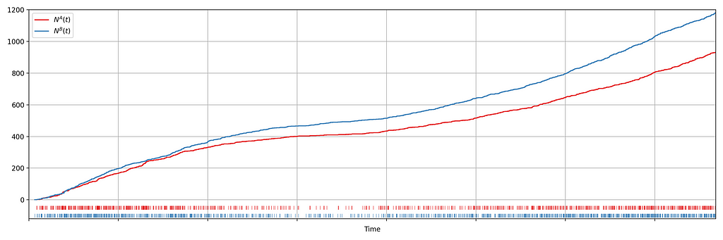
It is not immediately obvious by simple inspection of the point processes in Figure 1. The difference becomes immediately obvious when we visualize the observed counting processes, shown in Figure 2.
The counting processes are functions that increment by 1 whenever a new event arrives. Clearly, there are fewer events occurring in the treatment than in the control. If these were login events, this would suggest that the new code contains a bug that prevents some users from being able to log in successfully.
This is a common situation when dealing with event timestamps. To give another example, if events corresponded to errors or crashes, we would like to know if these are accruing faster in the treatment than in the control. Moreover, we want to answer that question as quickly as possible to prevent any further disruption to the service. This necessitates sequential testing techniques which were introduced in part 1.
Our data for each treatment group is a realization of a one-dimensional point process, that is, a sequence of timestamps. As the rate at which the events arrive is time-varying (in both treatment and control), we model the point process as a time-inhomogeneous Poisson point process. This point process is defined by an intensity function λ: ℝ → [0, ∞). The number of events in the interval [0,t), denoted N(t), has the following Poisson distribution
N(t) ~ Poisson(Λ(t)), where Λ(t) = ∫₀ᵗ λ(s) ds.
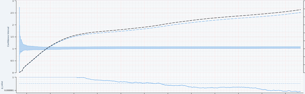
We seek to test the null hypothesis H₀: λᴬ(t) = λᴮ(t) for all t i.e. the intensity functions for control (A) and treatment (B) are the same. This can be done semiparametrically without making any assumptions about the intensity functions λᴬ and λᴮ. Moreover, the novelty of the research is that this can be done sequentially, as described in section 4 of our paper. Conveniently, the only data required to test this hypothesis at time t is Nᴬ(t) and Nᴮ(t), the total number of events observed so far in control and treatment. In other words, all you need to test the null hypothesis is two integers, which can easily be updated as new events arrive. Here is an example from a simulated A/A test, in which we know by design that the intensity function is the same for the control (A) and the treatment (B), albeit nonstationary.
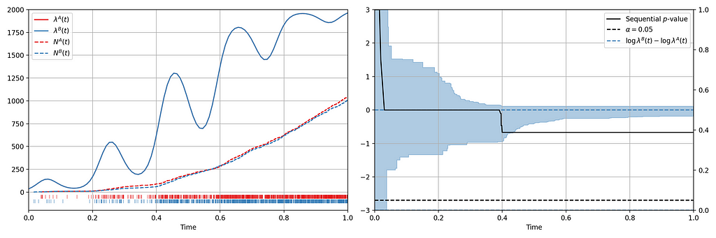
Figure 3 provides an illustration of an A/A setting. The left figure presents the raw data and the intensity functions, and the right figure presents the sequential statistical analysis. The blue and red rug plots indicate the observed arrival timestamps of events from the treatment and control streams respectively. The dashed lines are the observed counting processes. As this data is simulated under the null, the intensity functions are identical and overlay each other. The left axis of the right figure visualizes the evolution of the confidence sequence on the log-difference of intensity functions. The right axis of the right figure visualizes the evolution of the sequential p-value. We can make the two following observations
Now let’s consider an illustration of an A/B setting. Figure 4 shows observed arrival times for treatment and control when the intensity functions differ. As this is a simulation, the true difference between log intensities is known.
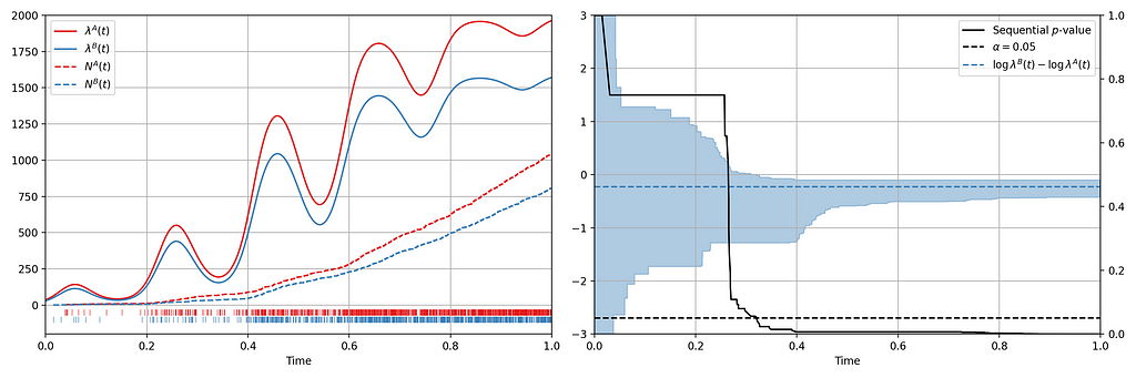
We can make the following observations
Now we present a number of case studies where this methodology has rapidly detected serious problems in a number of count metrics
Figure 2 actually presents counts of title start events from a real canary test. Whenever a title starts successfully, an event is sent from the device to Netflix. We have a stream of title start events from treatment devices and a stream of title start events from control devices. Whenever fewer title starts are observed among treatment devices, there is usually a bug in the new client preventing playback.
In this case, the canary test detected a bug that was later determined to have prevented approximately 60% of treatment devices from being able to start their streams. The confidence sequence is shown in Figure 5, in addition to the (sequential) p-value. While the exact units of time have been omitted, this bug was detected at the sub-second level.
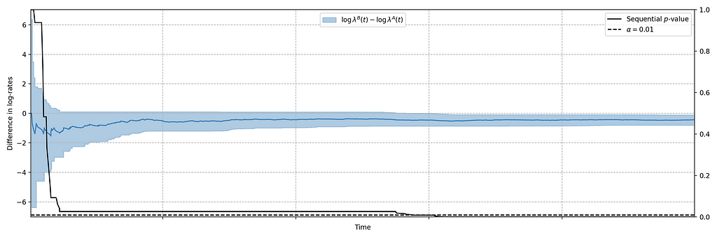
In addition to title start events, we also monitor whenever the Netflix client shuts down unexpectedly. As before, we have two streams of abnormal shutdown events, one from treatment devices, and one from control devices. The following screenshots are taken directly from our Lumen dashboards.
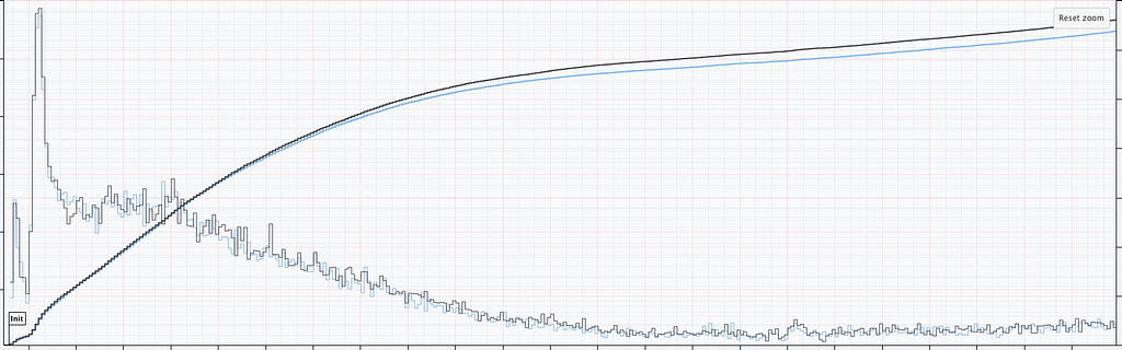
Figure 6 illustrates two important points. There is clearly nonstationarity in the arrival of abnormal shutdown events. It is also not easy to visibly see any difference between treatment and control from the non-cumulative view. The difference is, however, much easier to see from the cumulative view by observing the counting process. There is a small but visible increase in the number of abnormal shutdowns in the treatment. Figure 7 shows how our sequential statistical methodology is even able to identify such small differences.
Netflix also monitors the number of errors produced by treatment and control. This is a high cardinality metric as every error is annotated with a code indicating the type of error. Monitoring errors segmented by code helps developers diagnose issues quickly. Figure 8 shows the sequential p-values, on the log scale, for a set of error codes that Netflix monitors during client rollouts. In this example, we have detected a higher volume of 3.1.18 errors being produced by treatment devices. Devices experiencing this error are presented with the following message:
“We’re having trouble playing this title right now”
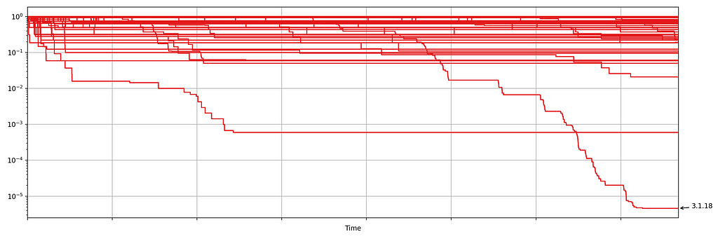
Knowing which errors increased can streamline the process of identifying the bug for our developers. We immediately send developers alerts through Slack integrations, such as the following
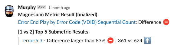
The next time you are watching Netflix and encounter an error, know that we’re on it!
The statistical approach outlined in our paper is remarkably easy to implement in practice. All you need are two integers, the number of events observed so far in the treatment and control. The code is available in this short GitHub gist. Here are two usage examples:
> counts = [100, 101]
> assignment_probabilities = [0.5, 0.5]
> sequential_p_value(counts, assignment_probabilities)
  1

> counts = [100, 201]
> assignment_probabilities = [0.5, 0.5]
> sequential_p_value(counts, assignment_probabilities)
  5.06061172163498e-06
The code generalizes to more than just two treatment groups. For full details, including hyperparameter tuning, see section 4 of the paper.
![]()
Sequential Testing Keeps the World Streaming Netflix Part 2: Counting Processes was originally published in Netflix TechBlog on Medium, where people are continuing the conversation by highlighting and responding to this story.
Post Syndicated from The History Guy: History Deserves to Be Remembered original https://www.youtube.com/watch?v=UMvlEgjPm9M
Post Syndicated from Bruce Schneier original https://www.schneier.com/blog/archives/2024/03/drones-and-the-us-air-force.html
Fascinating analysis of the use of drones on a modern battlefield—that is, Ukraine—and the inability of the US Air Force to react to this change.
The F-35A certainly remains an important platform for high-intensity conventional warfare. But the Air Force is planning to buy 1,763 of the aircraft, which will remain in service through the year 2070. These jets, which are wholly unsuited for countering proliferated low-cost enemy drones in the air littoral, present enormous opportunity costs for the service as a whole. In a set of comments posted on LinkedIn last month, defense analyst T.X. Hammes estimated the following. The delivered cost of a single F-35A is around $130 million, but buying and operating that plane throughout its lifecycle will cost at least $460 million. He estimated that a single Chinese Sunflower suicide drone costs about $30,000—so you could purchase 16,000 Sunflowers for the cost of one F-35A. And since the full mission capable rate of the F-35A has hovered around 50 percent in recent years, you need two to ensure that all missions can be completed—for an opportunity cost of 32,000 Sunflowers. As Hammes concluded, “Which do you think creates more problems for air defense?”
Ironically, the first service to respond decisively to the new contestation of the air littoral has been the U.S. Army. Its soldiers are directly threatened by lethal drones, as the Tower 22 attack demonstrated all too clearly. Quite unexpectedly, last month the Army cancelled its future reconnaissance helicopter which has already cost the service $2 billion—because fielding a costly manned reconnaissance aircraft no longer makes sense. Today, the same mission can be performed by far less expensive drones—without putting any pilots at risk. The Army also decided to retire its aging Shadow and Raven legacy drones, whose declining survivability and capabilities have rendered them obsolete, and announced a new rapid buy of 600 Coyote counter-drone drones in order to help protect its troops.
Post Syndicated from BeardedTinker original https://www.youtube.com/watch?v=Eatl4mNcb9g