Признанието като самопризнание

Post Syndicated from Дарина Сарелска original https://www.toest.bg/priznanieto-kato-samopriznanie/

Това е признание за всички вас. За българските медии, които предоставят територия за многоликото ни общество и възможности за диалог. 

Признанието като самопризнание

С тези думи Кирил Вълчев обясни защо е приел поканата на Илияна Йотова да се кандидатира за неин вицепрезидент. С което стана поредният в списъка с бивши журналисти, пристанали на моментен политически интерес. Бивш, защото през 2021 г. оглави БТА и така излезе от активната журналистика, която допреди това пак съвместяваше с друга професия – освен водещ на „Седмицата“ по Дарик радио беше и юридически консултант на медията (това само по себе си е особен хибрид, но да не придиряме). 

Иначе в кампанията ще си е напълно настоящ шеф на БТА, макар и в неплатен отпуск. Да, точно така, журналистите от БТА ще отразяват „безпристрастно“ и „равноотдалечено“ кампанията на своя началник, който съвсем реално може да се завърне в кабинета си на „Цариградско шосе“, ако „Дондуков“ се окаже негостоприемен. Но отразяването, разбира се, ще е професионално. Все пак няма да ни е за първи път! Пак така професионално преди две години Петър Волгин изкара една кампания в неплатен отпуск, преди да прескочи от журналист на общественото БНР до народен представител на „Възраждане“ в Европарламента. 

„Няма места.“ Журналистиката след журналистите

Ако се чудите какво стана с медиите в България, този текст ви е напълно достатъчен, за да си дадете отговори на много въпроси. А иначе, вие въпроси може и да си задавате, но в много медии у нас вече няма кой да ги задава – гледайте какво нещо… Защо стана така – от Дарина Сарелска.

От Клара Маринова до Антон Хекимян

От 1990 г. до днес поне една дузина разпознаваеми журналисти от БТА, БНТ, БНР, bTV, TV7, Nova и други национални медии преминават в политиката – като депутати, евродепутати, кметове или кандидати за президент. За същото това време доверието на българските граждани в новините чертае последователен и устойчив спад: според последния доклад на Института „Ройтерс“ то пада до рекордно ниските 21%, което е срив от 5 процентни пункта само за година. С това страната ни се нарежда сред държавите с най-ниско доверие в медиите, два пъти по-ниско спрямо средните стойности в глобален мащаб.

Не твърдя, че има причинно-следствена връзка. Но връзка има. И трябва да сме слепи, за да не видим дебелата не-винаги-червена линия, която разделя обществото на себеобслужващи се елити и пренебрегната и подценена публика. Когато аудиторията види „днес си водещ/директор, утре си кандидат на властта“, „днес интервюираш премиера в поза „уж критичен журналист“, а утре се снимаш с него в предизборен клип“ това размива доверието не само в конкретния човек, а в цялата система. 

Защото журналистиката по дефиниция е срещу властта. Не против конкретна партия, а срещу всяка власт. 

Добрата журналистика винаги е критична, проверяваща и възпираща нагона на властта. Когато водещи медийни лица преминават от другата страна на тази желязна завеса, това девалвира освен техните авторитетни имена – най-ценното им, пак по думите на Вълчев, но и самата идея за журналистиката като критичен агент и обществен контрол. 

И нека не се чудим защо тази година социалните мрежи настигнаха телевизиите като предпочитан източник на новини за българите, а догодина се очаква и да ги задминат. С всички мрачни последствия от това под формата на заливаща ни пропаганда, конспиративни теории, поляризация, радикализация и обикновено Дънинг-Крюгер оглупяване. Последствия, които берем къде с наивна детска изненада, къде с високомерната претенция за интелектуално превъзходство.

Но добре ще е следващия път, като се яви някой Тръмп или местен искащ-да-бъде-важен и получи залпова обществена подкрепа само защото „всички други са маскари“, да спрем за малко, преди да отсъдим. Да не бързаме със заключението „Ето, хората са прости“. И да погледнем дали наистина не се препълни с маскари, и то в редиците на елитите: умните, добре артикулираните, медийно симпатичните емблеми на всякакви кръгове, гилдии и общества, брандирани с признание и статус. Натрупали социален капитал под значката „равноотдалечени от всяка власт“ и скочили скоропостижно в листите на точно всяка власт, която ги пожелае.

Краят на журналистиката

Журналистиката губи не само пари и трафик, а и необходимостта да я има. Алгоритми, нюзинфлуенсъри и политици, които вече говорят директно на публиката, променят правилата на играта. Въпросът вече e не дали медиите са в криза, а дали обществото изобщо още иска журналистика. От Дарина Сарелска.

Първата вълна

Моделът „журналисти, преминали под партиен пагон“ не е нов. И не е само наш. Но у нас се вижда ясно в две вълни: първата – в края на 90-те, когато голямата политическа промяна трябва да се захрани с доверието, инвестирано в разпознаваеми лица и имена от единствените дотогава държавни медии, основно БНТ; втората – след 2005 г., когато частните телевизии стават стартова площадка за политически проекти.

В първата вълна се помнят имената на спортната журналистка Клара Маринова, после депутатка от БСП, както и на Асен Агов и Диляна Грозданова. Грозданова успява да сбъдне мечтата на всеки опортюнист и прави завъртане на 360 градуса. Първо взема завоя от емблематично лице на БНТ към политиката като пиар на Стефан Софиянски, влиза и сред учредителите на партията му „Съюз на свободните демократи“; след това застава и на депутатската банка (2001–2005) в редиците на НДСВ, а после се връща в медиите като изпълнителна директорка и водеща на частната TV7, чийто собственик тогава е съпругът ѝ Любомир Павлов. 

Асен Агов пък минава през БТА, БНР и БНТ, където стига до директор на новините, а после и на цялата телевизия след идването на власт на СДС (1992–1993). За да няма никакви съмнения кои са двигателите зад кариерното му развитие, е уволнен веднага след падането на правителството на Филип Димитров и преминава в активна политическа кариера с дълга поредица депутатски мандати от листата на СДС. Години след него този висш пилотаж пробва и Антон Хекимян, но стигна само до поста общински съветник от ГЕРБ в София.

Да, ама не

Единствен Петко Бочаров казва своето прословуто „Да, ама не“ на предложенията за политическа кариера. Дългогодишен журналист в БТА, по-късно зам.-главен редактор, добил популярност през 80-те като лице на предаването „Всяка неделя“, през 1991 г. е предложен за депутат от СДС, но отказва, защото смята депутатстването за несъвместимо с журналистическата си роля. Запомнете това. Защото е 

първият документиран публичен дебат в България за конфликта на интереси между медийна и политическа роля след промените. И първият публичен отказ. Следват тихи отлагания или признателни съглашателства. 

Между другото, Петко Бочаров е сред малкото публични личности с минало на сътрудници на Държавна сигурност, които сами го изваждат на светло, преди то да бъде огласено официално, и се разкайват за това. Изглежда, интегритетът понякога позволява на човек да демонстрира доблестно поведение дори с подобна биография. Обратното обаче също важи: фактът, че името ти никога не е било в архивите на един мракобесен апарат, сам по себе си не те прави по-достоен.

Да не се посочваме!

Властта в България може да се смени, да се прекръсти на „прогресивна“ и да обещае нов обществен договор, но едно остава непроменено – страхът от журналистически въпроси. А когато медиите са заключени в мазето, „демокрацията“ неизбежно започва да си говори сама със себе си. От Дарина Сарелска.

Частните телевизии като политически стартови площадки

Периодът на ширпотребата идва със зората на частните телевизии. Пионери са Волен Сидеров и неговата проруска партия „Атака“, която се ражда като политически проект от едноименното предаване на Сидеров по телевизия СКАТ, а само няколко години по-късно се изкачва до четвърта политическа сила в 40-тото Народно събрание.

Николай Бареков се опитва да повтори модела през 2014 г. След седем години, в които гради образа си в най-гледания сутрешен блок – на bTV, и то в най-силните години на телевизията, за кратко става началник в TV7 на банкера Цветан Василев, който тогава все още е в съдружие с Делян Пеевски. На 25 януари 2014 г. Бареков учредява партия „България без цензура“, с която достига до мандат в европарламента. Бареков е може би най-яркият пример за употребата на медия като политически трамплин. По-късно сам заявява: „Аз помогнах на Пеевски да разврати медиите“ – самопризнание, което независимо от мотивацията илюстрира дълбочината на проблема.

Интересното е, че по пътя си Бареков успява да приласкае и друг влиятелен за времето си телевизионен журналист – Росен Петров, който обръща палачинката на живо в ефира на bTV. По време на интервюто си с политика Бареков в предаването си „Нека говорят“ на 9 февруари 2014 г. водещият Петров подарява на госта си своята офицерска сабя и му се врича във вярност в ефир, като напуска телевизията с изчитане на нарочна декларация, за да се влее в редиците на Барековата партия. Без цензура. Един от най-срамните моменти, записани от камера в най-новата ни телевизионна история, е все още достъпен в интернет, макар и не на страницата на bTV, насладете се. 

Списъкът продължавa с Елена Йончева, Тома Томов, водещите от Nova Калина Крумова (започнала кариерата си от СКАТ) и Цвета Кирилова, Александър Симов и така до Антон Хекимян и Петър Волгин. През 2023 bTV поне от кумова срама изпрати Хекимян на партийна служба, приемайки оставката му с „незабавен ефект“ и демонстрирайки престорена институционална чувствителност към репутационния риск.

За да гаси имиджовия пожар тогава, телевизията обеща външен мониторинг на обективността на новините и актуалните предавания. Не се чу какво е установила тази проверка. Макар другата проверка – публичната, Хекимян системно да не издържаше години преди това, утвърждавайки се като предпочитан интервюиращ на Бойко Борисов, който в най-мрачните времена на брутално политическо превземане на прокуратурата започваше интервютата си с главния прокурор Цацаров с въпроса какво значи името Сотир (значи „спасител“) и с покана да сподели кого последно бил спасил от кабинета си в Съдебната палата. Това само му вдигна цената до шеф на новините и неуспял кандидат-кмет на ГЕРБ. 

И така до днес, когато никой не се скандализира при прескачането на шефовете на медии в политиката. Няма нужда да се правят проверки наужким, нито да се мятат оставки. Просто си пускаш неплатен. Така Кирил Вълчев е и възможен, и направо закономерен кандидат за вицепрезидент, а в инициативните комитети се прескачат журналист през журналиста – от Константин Вълков при Андрей Гюров, до Валерия Велева, Кристина Патрашкова и Явор Дачков при Илияна Йотова. 

Има за всички. Хубаво е, и е готово

Хубавото е, че става видимо. Журналисти с двойно предназначение се самоосветяват, заемайки видими публични позиции. Тази прозрачност, макар да убива доверието в професията, все пак е и малко полезна. Защото вдига завесата пред тези авторитети под прикритие. Разбира се, не бива да сме наивни – със сигурност се отглеждат приемливи фасади от ново поколение. А и границата отдавна е твърде размита. 

Да, между журналистиката и политическата власт трябва да има защитна стена. 

За съжаление, все по-често тя прилича на въртяща се врата. Съвсем нормализирана е вече практиката действащи журналисти да предлагат медийни обучения и консултантски PR услуги – и на корпоративни, и на партийни клиенти. Защо пък да не водят направо и собствените си кампании от студиата на новините!

Къде е границата? 

Журналистите, разбира се, могат и е нормално да бъдат политически хора – с убеждения, с позиция, с обществен ангажимент. Безпристрастността не означава безразличие. Границата минава другаде – 

да не злоупотребяваш с капитала на собственото си доверие. Да не го търгуваш, да не го превръщаш в разменна монета за пост или привилегия. 

Журналистите имат право на гражданска активност, дори и на граждански протест – защото това е лична позиция. Не злоупотреба или тайно превалутирано доверие в полза на кампания или на конкретен политически интерес. Стандартът за конфликт на интереси и недопускане на пристрастност е описан ясно и с примери в принципите на Associated Press – световния аналог на БТА, с който родната агенционна журналистика иначе обича да се сравнява:

От служителите в редакцията се очаква стриктно да избягват всякаква политическа дейност, независимо дали редовно отразяват политика, или не. Те не могат да се кандидатират за политически длъжности или да приемат политически назначения, нито да извършват дейност по връзки с обществеността за политици или техни организации. При никакви обстоятелства не бива да даряват средства на политически организации или за политически кампании. Те трябва да преценяват особено внимателно дали да членуват, или да правят дарения в други организации, които могат да заемат политически позиции.

Дори служителите извън редакцията – разбирайте счетоводители, шофьори и юрисконсулти, трябва да се въздържат от политическа дейност и от дарения, освен ако не получат одобрение от прекия си ръководител. Ограничения има даже за членовете на техните семейства, чиито политически каузи и ангажименти също подлежат на публично деклариране. 

Разбира се, преквалификацията на журналисти в политици не е само роден феномен – справка: от Мусолини, през Уинстън Чърчил, до Борис Джонсън. Но и тук има нюанс и той е в наличието на т.нар. охлаждащ период. 

Има ли кой да ги накаже? За забранителните списъци в bTV и кебапчетата в медиите

Имало едно време един Асен. Вървял, вървял през девет телевизии в десета и попаднал в bTV, където решил, че ще е „яли, пили и се веселили“, докато той каже и само с когото той прецени. Извинявайте, но няма нищо приказно в тази история. От Дарина Сарелска.

Липса на „охлаждащ период“ 

Според етичните стандарти в много страни, когато журналист става политик, се изисква, или поне силно се препоръчва, пауза между двете роли, за да не се компрометира доверието в медиите. Нали заради това доверие се търсят подобни кандидати все пак?! Не е много умно да се реже клонът, на който седиш. 

Така преходът е плавен и бившите журналисти стават политици обикновено след като вече са изградили партийна кариера (говорители, съветници, експерти). Такъв е примерът и на самата Илияна Йотова, която е доста последователна в кариерната си траектория: започва като репортер, налага се като разпознаваемо лице в БНТ, после оставя журналистиката зад гърба си, заема се с комуникациите на БСП, откъдето бавно, полека и отвътре изгражда партийна кариера, за да стигне днес до президент. Това е класическият и по-приемлив път. При Вълчев и при повечето български примери преходът изглежда рязък: от днес за утре. Без междинни стъпки в партийната йерархия или време за хигиенна дистанция. Нещо като да вдигнеш сватба, преди комшиите да са разбрали, че си се развел.

Но да се върнем към (само)признанието на Кирил Вълчев: 

Приемам поканата на президента като признание не за мен, а за БТА – институция на съгласие, на общуване с българите по света, на памет, нещо, от което има нужда в Президентството.

А Илияна Йотова допълва: 

Дълги години имаме обща кауза с господин Вълчев. Работихме заедно за тази кауза – за опазване на българщината, за развитието на българската идентичност, на българския дух, на българската писменост, на буквите.

Да, от такава БТА има нужда Президентството. От такива медии имат нужда всички овластени. Институции на дългогодишното съгласие. Медии, тихи за злоупотребите на властта и споделящи шумно нейните каузи – днес буквите и българщината на „Прогресивна България“, вчера евроатлантизмът ала ГЕРБ и ДПС – Ново начало, утре – каквото нуждата покаже. Стига да е споделена. 

Good night, and good luck, motherf*ckers

Историята на американското предаване „60 минути“ е разказ за механизмите, чрез които се опитомяват медиите. И тези механизми са удивително сходни, независимо от пазара или знамето пред сградата на телевизията. Един текст в стил „Думам ти, дъще, сещай се, журналистическа снахо“ от Дарина Сарелска.

А журналистиката – тя отдавна е пратена в отпуск. Обикновено платен. Така стигаме до реалността, в която нищо не е вярно и всичко е възможно. Времена, в които всеки, който има YouTube канал, се пише журналист. Всеки, който е натрупал два грама доверие като журналист, може да го капитализира за политически пост. Всеки новоизлюпен политик може да привижда в собствените си котерии обществения интерес, обяснявайки ни как „работи за хората“. А пък хората гледат „Ергенът“. Може би там някъде е бъдещият спасител. 
AIs Compress Exploit Timeline

Post Syndicated from Bruce Schneier original https://www.schneier.com/blog/archives/2026/09/ais-compress-exploit-timeline.html

Give an AI agent a mere rumor of an exploit, and it’s enough for them to find it.

What’s worse, I found I could use my own agents to find the exploit just by knowing roughly what it was about and so could have been exploiting it well before the public patch was available! Given that just the rumour of a security issue seems enough to give attackers enough info to find new exploits, we’re going to need to change the way we deal with security responses in open source.

Simon Willison comments:

Anil points out that this rate of discovery appears incompatible with existing open source embargo practices for new issues. If an issue can become an exploit this fast, we need to figure out new processes for keeping our communities safe.

Президентски избори 2026 – заявление за гласуване

Post Syndicated from Боян Юруков original https://yurukov.net/blog/2026/pres2026-zayavlenie/

Тази информация беше изпратена на над 3000 абонирали се за бюлетина на Glasvam.org заедно с новини и полезни съвети за подготовката и провеждането на гласуването в чужбина.


На 25-ти октомври 2026 ще се проведат избори за президент и вицепрезидент. Вече може да подавате заявление за гласуване зад граница. Ще намерите формуляра на страницата на ЦИК. Там може да проверите и дали правилно е записано заявлението ви. Ето няколко важни неща, които трябва да знаете:

  • Крайният срок за подаване е 29-ти септември в полунощ българско време
  • Подаването на заявление за гласуване в секцията най-близо до Вас, ще Ви улесни и ще ускори изборния процес, тъй като ще сте вече вписани в списъците
  • Заявление се подава за всеки вот поотделно. Т.е. не се пренасят от предходни избори
  • Дори да подадете заявление, а се окаже, че на 25-ти октомври сте в България, ще може да гласувате в секцията си по постоянен адрес с попълване на декларация
  • Вече са предварително одобрени 362 места за секции в чужбина, където в последните 5 години е имало поне 100 гласували. Те са в 293 града в 57 държави. Това е значително по-малко от предишни години, тъй като автоматичното одобрение на секции по чл. 14, ал. 2, т. 2 беше ограничено до рамките на Европейския съюз. По-малко е дори от преходните, където бяха силно ограничени секциите в чужбина.

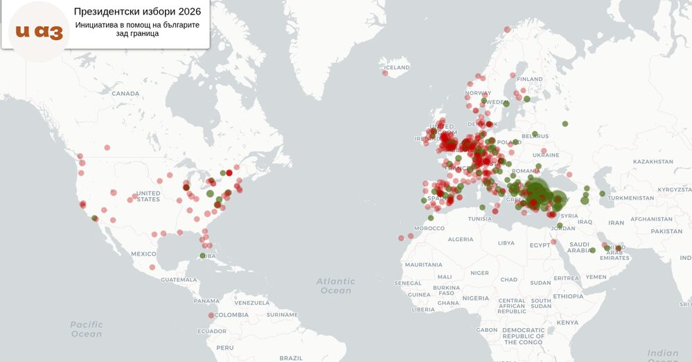
  • За отваряне на секции извън Европейския съюз остава единствено възможността да се съберат поне 40 заявления и след преценка на дипломатическите представителства. През 2026 г. поне отпаднаха ограниченията за броя секции извън ЕС, което засягаше основно Великобритания, Турция и САЩ. Това означава, че подаването на заявление е още по-важно от предходни години.
  • Автоматичното одобрение и събраните заявления не означава, че непременно ще има секции на тези места. Това зависи от възможностите на помещенията и дали има комисии и доброволци към тях. Решението е на ЦИК по препоръка на Външно. Могат да се увеличат шансовете като се подават заявления за тези места и повече хора се включат като членове на комисии и доброволци.
  • На някои места като Германия е нужно да се иска разрешение от местните власти. Това вече би трябвало да се случва предвид предварително одобрените места. Очакваме информация от МВнР
  • Подаването на заявления освен, че подпомага изборния процес, показва и повишен интерес на съгражданите ни в чужбина към вота

В началото на 2026 г. трябваше да се въведе избирателен район Чужбина с 4 депутата, които щяха да представляват единствено българските граждани зад граница. Тази възможност обаче беше отложена отново до януари 2028-ма в последния момент преди парламентарните избори в началото на годината. Повече по темата описах преди предишния вот.

Събирането на заявленията ще може да следите в реално време на картата, както и на подробната таблица. Възможно е автоматичното зареждане на данните да спре заради промени по сайта на ЦИК, каквито случаи имаше в последните години. Ще допълня, ако има промяна.

Customize Amazon API Gateway destinations for execution logs

Post Syndicated from Giedrius Praspaliauskas original https://aws.amazon.com/blogs/compute/customize-amazon-api-gateway-destinations-for-execution-logs/

Amazon API Gateway execution logs help you trace request processing step by step through your REST API stages. They capture authorization results, integration latency, mapping template output, and error details that are otherwise invisible at the API surface. When a production request fails in a way the access log cannot explain, the execution log is usually where you find the explanation.

Until now, execution logs had two constraints. Every log event was truncated at 1 KB, so a request carrying a moderately sized JSON body would exceed that limit and the remainder was dropped. Logs could only go to the auto-managed log group that API Gateway creates for you (API-Gateway-Execution-Logs_{rest-api-id}/{stage_name}).

With Amazon CloudWatch Logs delivery for REST API execution logs, you can now route execution logs to Amazon CloudWatch Logs, Amazon Simple Storage Service (Amazon S3), or Amazon Data Firehose. Log events can be up to 1 MB per entry, and you benefit from vended logs pricing.

In this post, you learn how CloudWatch Logs delivery works with API Gateway execution logs, how to configure it, and what patterns work best for common observability scenarios.

Understanding API Gateway execution logs

API Gateway produces two categories of logs: access logs and execution logs. Access logs record a summary line per request, similar to an HTTP server access log. You configure the format and destination yourself.

Execution logs are different. They capture the internal processing of each request as it moves through the API Gateway pipeline: authorizer evaluation, request validation, integration dispatch, response mapping, and error handling. These logs exist so you can answer questions such as “why did my authorizer reject this token?” or “what did the mapping template produce before it reached my backend integration?”

API Gateway manages execution log creation automatically. When you set loggingLevel to INFO or ERROR in your stage’s method settings, the service writes execution log events to a CloudWatch Logs log group it manages on your behalf. You do not choose the log group name or configure retention directly on it.

The auto-managed model works for many customers but may create friction for teams with specific observability requirements. Compliance frameworks that require logs in S3 with a particular prefix structure need an extra subscription filter and delivery mechanism. Sending execution logs into a security information and event management (SIEM) tool through a Firehose stream requires a forwarding layer.

Configurable log delivery with CloudWatch Logs

CloudWatch Logs delivery separates log routing from log content. Two concepts control the behavior:

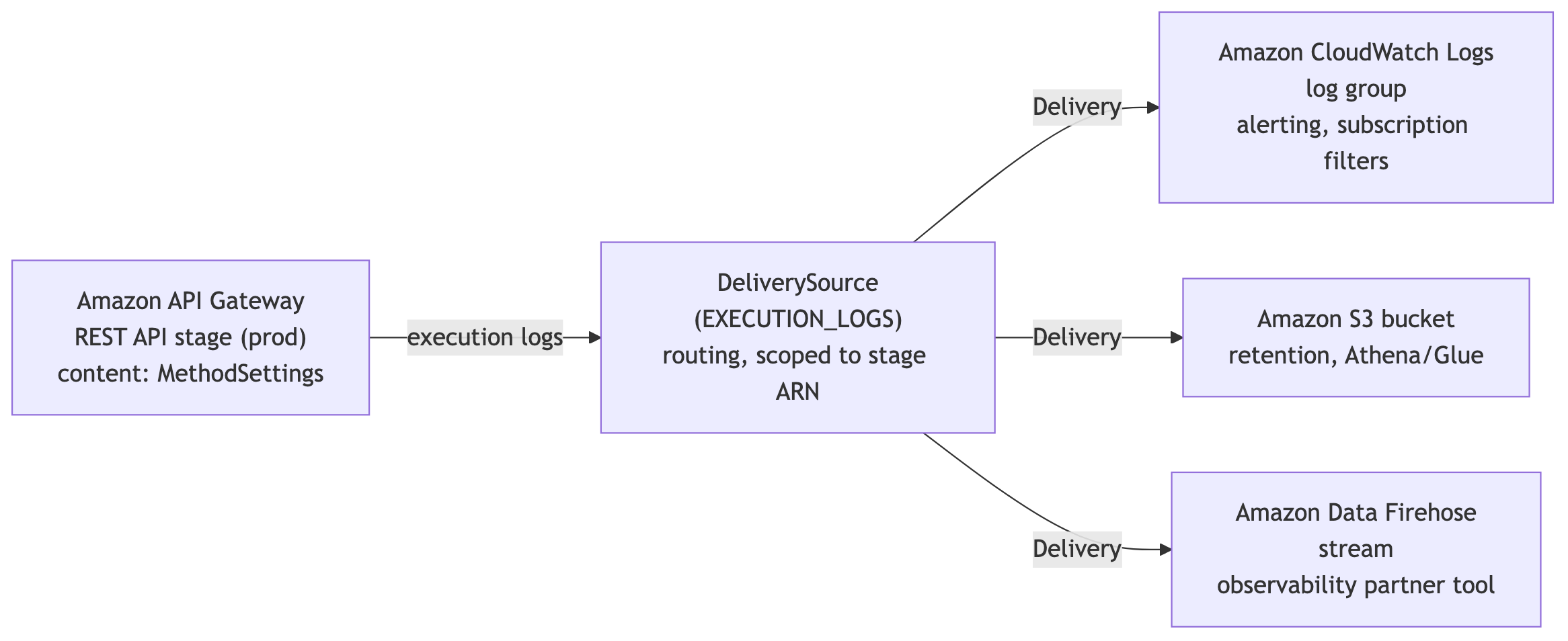
DeliverySource is scoped to your API Gateway stage ARN. It defines where logs go. You create a delivery source, then attach one or more delivery destinations (CloudWatch Logs log group, S3 bucket, or Firehose stream).

MethodSettings controls what gets logged. The loggingLevel setting (INFO, ERROR, or OFF) and dataTraceEnabled flag still determine which log events API Gateway produces. These settings work the same way regardless of whether you use the auto-managed log group or CloudWatch Logs delivery.

When you create a delivery using the CloudWatch Logs APIs, CloudWatch Logs activates your log delivery on your API Gateway stage. When you delete the delivery, CloudWatch Logs disables it accordingly. You do not need to flip any flags on the API Gateway side, and the execution logs automatically resume flowing to the auto-managed log group.

Your existing method settings keep their meaning. The loggingLevel and dataTraceEnabled values continue to control log content. If loggingLevel is already INFO or ERROR, creating a delivery redirects those logs to your chosen destination with no further configuration.

The following diagram shows how the pieces fit together.

Diagram showing one API Gateway stage delivery source fanning out to CloudWatch Logs, Amazon S3, and Firehose destinations.

Figure 1 — A single delivery source scoped to an API Gateway stage feeds one or more deliveries, each of which writes to a delivery destination backed by CloudWatch Logs, Amazon S3, or Amazon Data Firehose

The following table summarizes what changes when log delivery is active.

Aspect Standard execution logging Log delivery
Destination Auto-managed CloudWatch Logs log group CloudWatch Logs, Amazon S3, or Firehose
Multi-destination No Yes
Pricing Standard CloudWatch Logs ingestion Vended logs pricing
Log event size Truncated at 1 KB Up to 1 MB
Setup Set loggingLevel in MethodSettings Create delivery through CloudWatch Logs APIs
Teardown Set loggingLevel to OFF Delete delivery

What stays the same

Only execution log routing changes. Access logs continue to flow through accessLogSettings to whatever log group you configure, and unrelated stage features such as AWS X-Ray tracing, detailed CloudWatch metrics, throttling, and caching behave exactly as they did before.

Configuration and integration options

Before you create a delivery, confirm the following requirements:

  • The API Gateway REST API is deployed to a stage.
  • loggingLevel is set to INFO or ERROR in MethodSettings.
  • The account-level CloudWatch Logs IAM role is configured. For setup steps, see Set up CloudWatch logging for REST APIs in API Gateway.
  • For cross-account delivery, the destination has an appropriate resource policy attached through PutDeliveryDestinationPolicy.

Sending logs to a custom CloudWatch Logs log group

The most common starting point is redirecting execution logs to a log group you own. You get direct control over retention policies, metric filters, and subscription filters. The following steps use the AWS Command Line Interface (AWS CLI) with the fictitious REST API ID abc123, stage prod, Region us-east-1, and account 111122223333.

  1. Create a delivery source referencing your stage ARN. The log type for REST API execution logs is EXECUTION_LOGS:
    aws logs put-delivery-source \
        --name my-apigw-execution-logs \
        --resource-arn arn:aws:apigateway:us-east-1:111122223333:/restapis/abc123/stages/prod \
        --log-type EXECUTION_LOGS

  2. Create a delivery destination pointing to your custom (existing) log group, then create the delivery that connects them:
    aws logs put-delivery-destination \
        --name my-execution-log-destination \
        --delivery-destination-configuration \
            destinationResourceArn=arn:aws:logs:us-east-1:111122223333:log-group:/my-api/execution-logs

    aws logs create-delivery \
        --delivery-source-name my-apigw-execution-logs \
        --delivery-destination-arn arn:aws:logs:us-east-1:111122223333:delivery-destination:my-execution-log-destination

  3. Verify that the delivery is active by listing deliveries for the source:
    aws logs describe-deliveries

The response includes the delivery ID, source, and destination ARN after delivery is established. Execution logs flow to /my-api/execution-logs instead of the auto-managed group.

Note: Log delivery adds structured fields (resource_arn, event_timestamp, api_id, stage, resource_path, http_method, and payload) to each event, so a new delivery emits more than your previous logs. To keep the traditional execution log format with nothing extra, set output format and record fields while creating delivery destination and creating delivery:

aws logs put-delivery-destination \
    --output-format "plain" ...

aws logs create-delivery \
    --record-fields "payload" \
    --field-delimiter "" ...

Routing logs to Amazon S3

S3 works well for long-term retention at lower cost, or for feeding logs into analytics tools such as Amazon Athena. The bucket must be in the same region as your API. Create a delivery destination pointing to your bucket:

aws logs put-delivery-destination \
    --name s3-archive-destination \
    --delivery-destination-configuration \
        destinationResourceArn=arn:aws:s3:::amzn-s3-demo-apigw-logs

Then create a delivery using the same source name. CloudWatch Logs delivers the events to your bucket, where you can query them with Athena or catalog them with AWS Glue.

Streaming to Amazon Data Firehose

For real-time analytics pipelines or third-party SIEM integration, Firehose delivery sends execution log events directly to your stream. The setup is identical: create a delivery destination with your Firehose stream ARN, then create a delivery. With direct Firehose delivery, you no longer need to maintain CloudWatch Logs subscription filters and AWS Lambda forwarders to route execution logs to external analytics systems.

Multi-destination delivery and per-destination shaping

A single delivery source supports multiple destinations. You can route the same execution logs to CloudWatch Logs for real-time alerting, S3 for long-term compliance retention, and Firehose for your SIEM, all from one stage. Create additional deliveries using the same delivery source with different destination ARNs.

Each destination receives identical log events. To shape what reaches each destination, apply a CloudWatch Logs subscription filter on the CloudWatch Logs destination. For example, you can forward only ERROR-level events to a Lambda function that pushes alerts to a SIEM, while the same delivery source writes the full event stream to S3 for compliance.

Management console experience

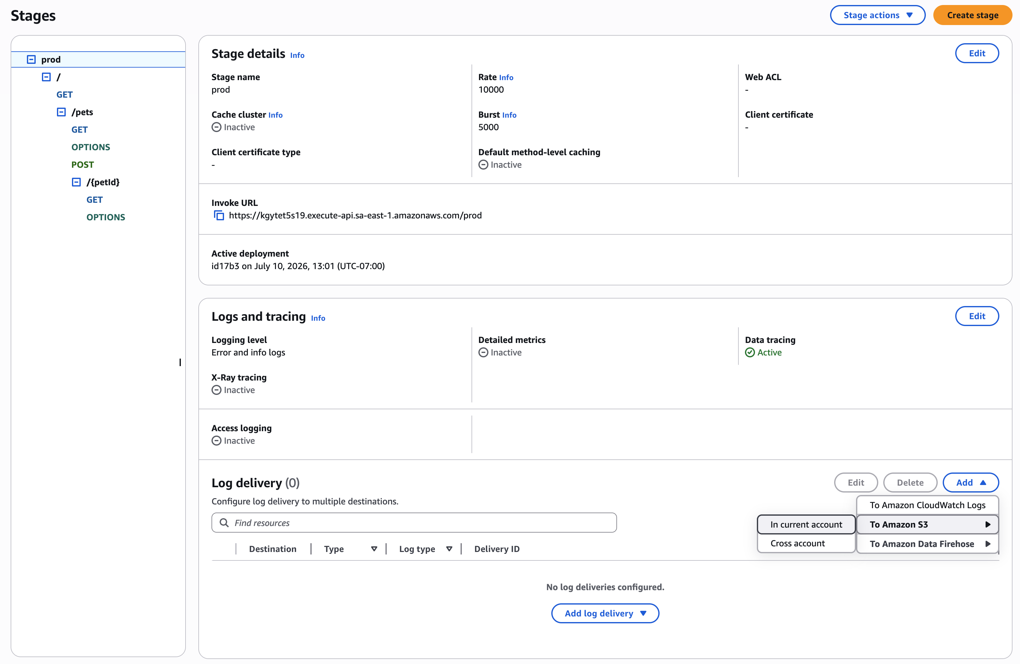
You can also add a log delivery destination in the management console after you enable logging for the stage.

API Gateway console showing the option to add a log delivery destination after logging is enabled for the stage.

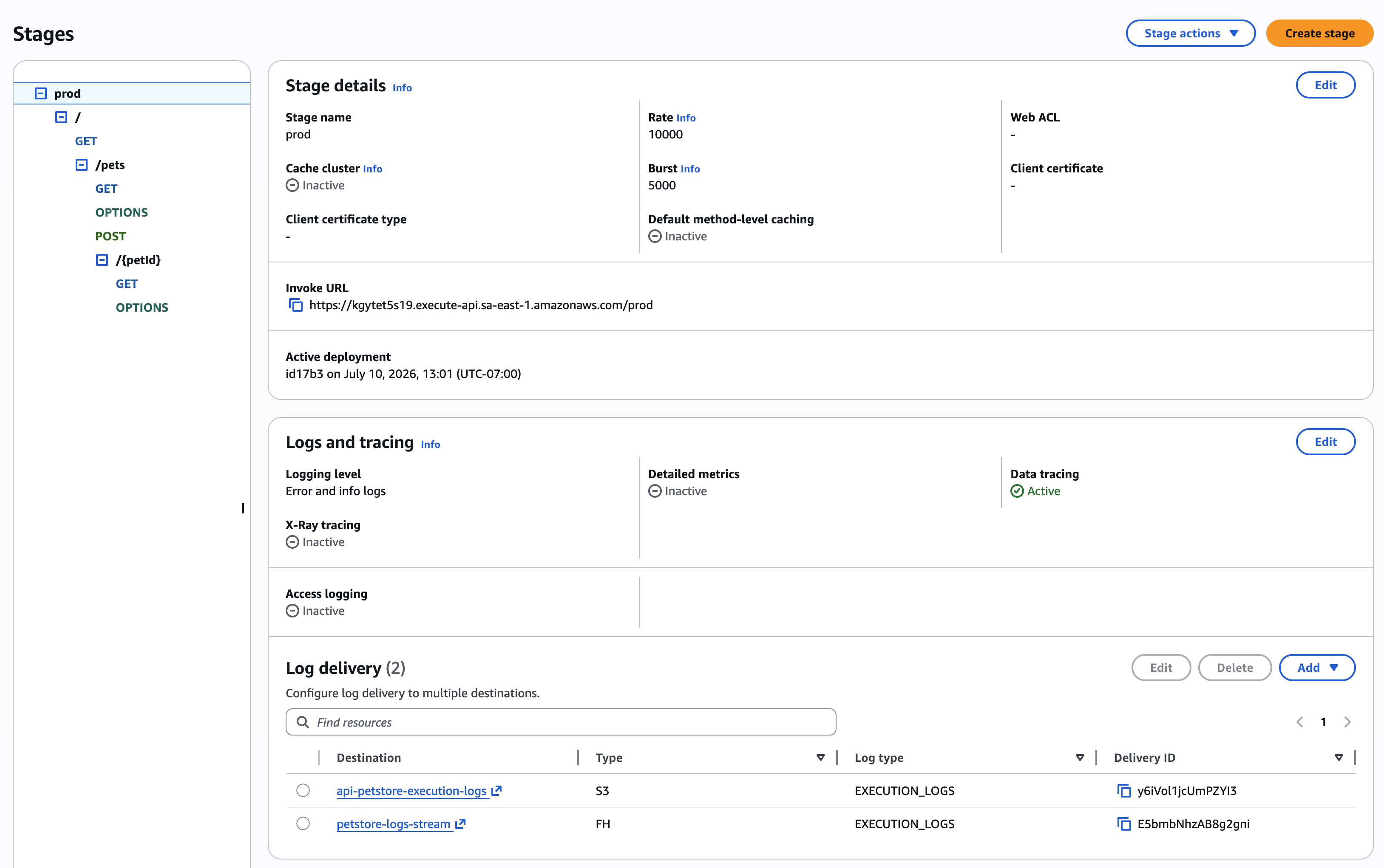
You can specify multiple destinations, both in the current or in a different account:

API Gateway console showing multiple delivery destinations configured, including cross-account options.

Keeping existing monitoring intact

If you have dashboards or alarms on the auto-managed log group, use that same log group as one of your delivery destinations. Your existing monitoring keeps working, and you gain the ability to send logs to additional destinations such as S3 or Firehose in parallel.

Best practices

Update dashboards and alarms before enabling log delivery. When you activate log delivery, the auto-managed log group stops receiving logs. Any CloudWatch alarms, dashboards, or Contributor Insights rules pointing to API-Gateway-Execution-Logs_{rest-api-id}/{stage_name} stop working. Migrate these references to your new log group before creating the delivery.

Keep loggingLevel at INFO or ERROR. Log delivery controls routing, not content. If loggingLevel is OFF, no execution log events are produced regardless of whether a delivery exists. Verify your method settings before troubleshooting missing logs.

Treat the 1 MB log event capacity as a security decision, not only a debugging convenience. With dataTraceEnabled set to true, execution logs include complete request and response payloads up to 1 MB. Those payloads might contain personally identifiable information (PII) or other sensitive data. Confirm your log destinations have appropriate access controls, encryption, and retention policies. Mask or filter sensitive fields in mapping templates upstream of logging and enable data tracing selectively per method or only in non-production stages.

Start with a single destination, then expand. Validate that your log group or bucket receives events correctly before adding Firehose or additional destinations.

Log delivery is best-effort. In rare cases, some log events might not be delivered. For audit-critical workloads, build retention and reconciliation that account for occasional missing events rather than treating execution logs as the system of record.

Cleaning up

To avoid ongoing charges from the resources you created while following this post, delete the delivery and then remove the destinations and any example S3 bucket or Data Firehose delivery stream you no longer need. Deleting the delivery returns the stage to standard auto-managed logging.

aws logs delete-delivery --id <delivery-id>

When the delivery is deleted, CloudWatch Logs disables log delivery on the API Gateway stage automatically. The delivery source and delivery destination remain as independent objects. Delete them with delete-delivery-source and delete-delivery-destination if you do not plan to reuse them.

Conclusion

CloudWatch Logs delivery for API Gateway REST API execution logs helps address the 1 KB event truncation and single managed destination constraints. You can now route full execution logs to CloudWatch Logs, Amazon S3, or Amazon Data Firehose, use multiple destinations from a single stage, and pay vended logs pricing.

The feature works alongside existing method settings. No changes to your current logging configuration are required beyond creating the delivery itself.

To get started, refer to Route execution logs with Amazon CloudWatch Logs delivery in the API Gateway documentation. For more about CloudWatch Logs delivery configuration, see Enable logging from AWS services. For pricing details, review the Amazon CloudWatch pricing page. Try it on a test stage and share your experience in the comments.

Introducing Amazon EBS Volume Clones across AWS accounts

Post Syndicated from Channy Yun (윤석찬) original https://aws.amazon.com/blogs/aws/introducing-amazon-ebs-volume-clones-across-aws-accounts/

Last year, we introduced Volume Clones of Amazon Elastic Block Store (Amazon EBS), a new capability that lets you create instant point-in-time copies of your EBS volumes within the same Availability Zone.

Today, we are extending Volume Clones with cross-account copy, so you can create copies of your EBS volumes into other AWS accounts and optionally re-encrypt them with an AWS Key Management Service (AWS KMS) key in the target account.

With this new feature, you can use your latest application data to develop, test, and experiment in a secondary environment, while protecting and isolating the information in the production environment. For example, you can create copies of a production environment to refresh test and development environments set up in separate accounts with the desired EBS encryption.

Copy EBS volumes across AWS accounts in action
To create a copy of an EBS volume across accounts, the owners of the volume can first grant the target account access to their volume in AWS Resource Access Manager (RAM), which provides a way to share resources across AWS accounts or within an AWS Organization. Then, from the target account, they can locate the volume they have access to create a copy of it.

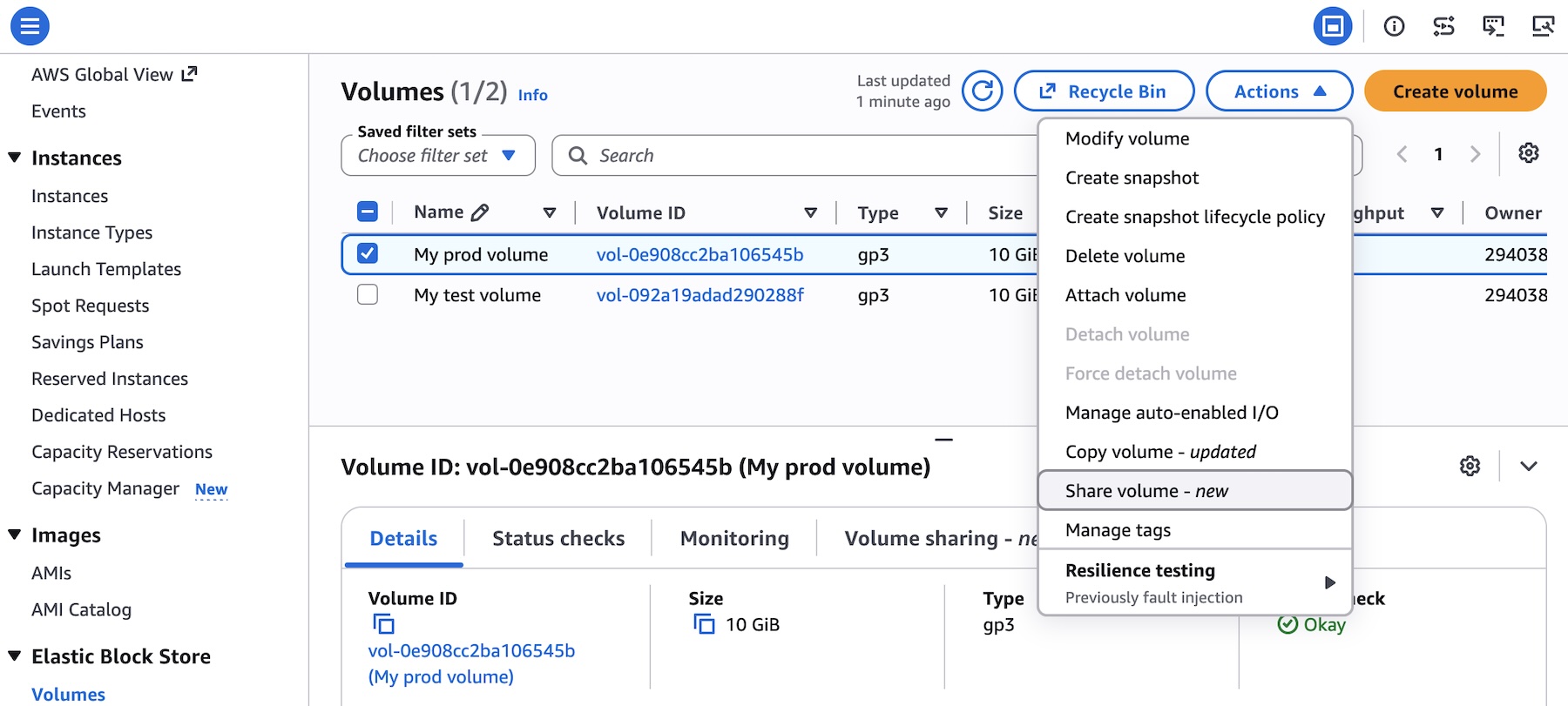
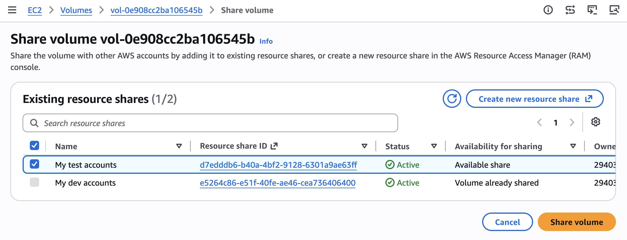
To get started, choose Share volume for the volume you want to share with the target account in the Amazon EBS console.

Share the volume with other AWS accounts by adding it to existing resource shares, or create a new resource share in the AWS RAM console. For more details, refer to the AWS RAM User Guide.

You can now see confirmation that the volume has been shared in the Volume sharing tab of the volume detail page.

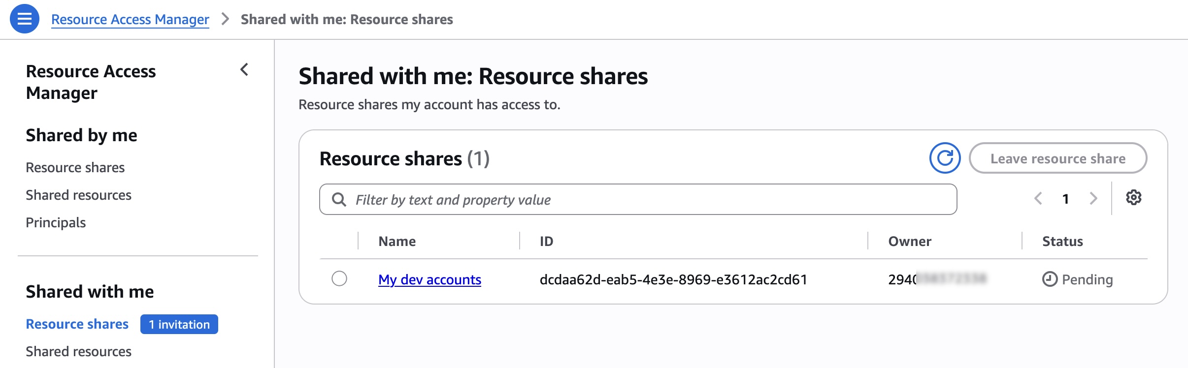
A target account must accept the resource share on the RAM console.

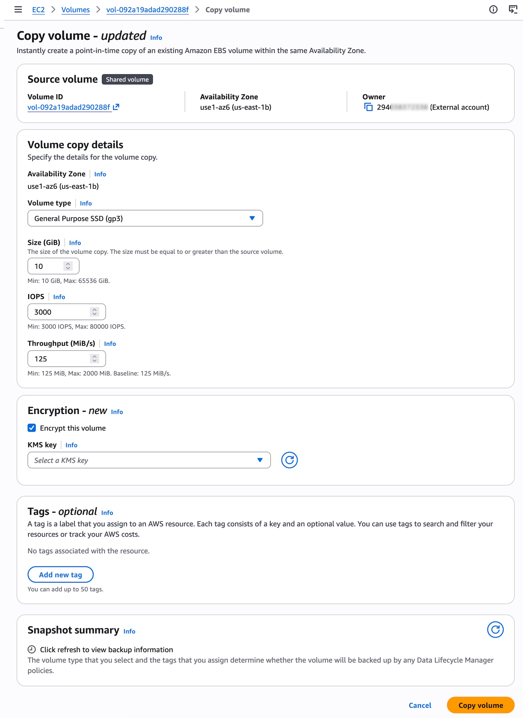
Once they accept the resource share, they can see the volumes in the EBS volume page of the target account. Choose Copy volume for any shared volume.

To share and copy EBS volumes across AWS accounts programmatically, including calling APIs and searching documentation, try the AWS MCP Server and plugins with your preferred AI coding tool. To learn more, visit the Amazon EBS User Guide.

Things to know
Let me share some important technical details that I think you’ll find useful.

  • Encryption: You can share unencrypted volumes and volumes encrypted with a customer managed key (CMK). Volumes encrypted with the default AWS managed key (AMK) cannot be shared. When copying a shared volume encrypted with a CMK, the CMK must also be shared with the target account. You can specify a different CMK to re-encrypt the copy in the target account.
  • Monitoring: You can monitor SharedVolumeCopyInitiated through AWS CloudTrail event in your account. You will also receive events in Amazon EventBridge at the start of the copy operation when the state of the copied volume is initializing, and at the end of the operation when the state of the copied volume changes to completed. You can see the shared volume ID, consuming account ID, and event time.
  • Pricing: Once a copy is initiated, you’ll pay a one-time fee based on your volume size, charged to the account where the copy will reside. There’s no cost for sharing EBS volumes through AWS RAM. The copied volume will incur regular EBS volume charges upon creation.
  • Availability Zone: The volume copy must be created in the same Availability Zone as the source volume. Use Availability Zone IDs (such as use1-az1) to identify the same physical location across accounts.

Now available
Cross-account volume clones for Amazon EBS are available in all AWS Regions that support Amazon EBS Volume Clones. For Regional availability and a future roadmap, visit the AWS Capabilities by Region.

Give this feature a try in the Amazon EC2 console today and send feedback to AWS re:Post for Amazon EBS or through your usual AWS Support contacts.

— Channy

Testing application resilience with Amazon SQS and AWS Fault Injection Service

Post Syndicated from Richard Whitworth original https://aws.amazon.com/blogs/architecture/testing-application-resilience-with-amazon-sqs-and-aws-fault-injection-service/

When your application can no longer send or receive messages through an Amazon Simple Queue Service (Amazon SQS) queue, downstream processing can stall. The cause might be a misconfigured Identity and Access Management (IAM) policy, a network partition, a bad deployment, or a transient service event. Your application sees much the same thing regardless: SQS operations start failing. How your services handle those failures (failing fast on what won’t succeed, opening circuit breakers, buffering on the producer side) can be the difference between a brief disruption and a cascading outage.

If you’ve never tested those mechanisms under failure, you’re relying on assumptions. With AWS Fault Injection Service (AWS FIS), you can find out first. The goal isn’t to verify that SQS works, it’s to learn what your application does when SQS operations fail, and whether you’d notice. A resilience experiment tests your recovery mechanisms and your observability at once.

In this post, you’ll learn how to:

  • Structure a resilience experiment with a clear, measurable hypothesis and success criteria.
  • Use AWS FIS and AWS Systems Manager (SSM) Automation to simulate progressive access disruption to SQS queues.
  • Interpret Amazon CloudWatch metrics to determine whether your resilience mechanisms are working, distinguishing producer-side from consumer-side behavior.
  • Identify and fix gaps in your application’s failure handling.

Solution overview

In this experiment, you block your application’s access to SQS with a scoped deny resource policy, then restore access and observe recovery. The policy you apply rejects the data-plane operations your application depends on (sending, receiving, deleting, and changing message visibility, plus purging) while leaving queue management untouched. Disruption duration increases across four phases to surface different classes of failure. To learn more, see Control planes and data planes.

Important: Don’t deny sqs:*. In IAM policy evaluation, an explicit Deny overrides every Allow, including the automation’s own permission to remove the policy later. A deny covering sqs:SetQueueAttributes, sqs:AddPermission, and sqs:RemovePermission can lock the queue so that even the role that applied it can’t clean it up. Scope the deny to data-plane actions only. See Configuring the experiment for the safe policy shape, SQS troubleshooting: access denied, and this re:Post article on deny-policy lockout.

You can find the fault-injection code (the SSM Automation document, the FIS experiment template, and example IAM policies for both roles) in the FIS template library on GitHub.

Progressive experiment phases

Short disruptions can reveal whether your failure-handling mechanisms activate. Longer ones can expose systemic issues that might only appear under sustained failure.

Note: This experiment tests your application’s resilience patterns, not SQS itself. The scoped deny simulates what your application would experience during a network partition, a permission change, or another access disruption.

You can watch two distinct failure surfaces at once:

Producer side: The component that calls SendMessage. When sends are denied, you’re testing how the producer handles failed enqueues: does it fail fast, open a circuit breaker, buffer locally, or drop messages?

Consumer side: The component that calls ReceiveMessage and DeleteMessage. When receives are denied, you’re testing backlog growth during the outage and, on recovery, redelivery and whether a consumer working through the accumulated backlog keeps up or starts pushing messages toward the DLQ.

To isolate a consumer outage instead, where a bad deployment or scaling issue stops your consumers while producers keep sending, deny only sqs:ReceiveMessage and sqs:DeleteMessage. This can be done by editing the SSM Automation document.

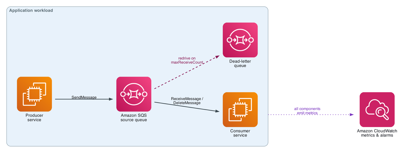
Producer service sends to an SQS queue, a consumer service reads from it, a dead-letter queue attaches to the source queue, and CloudWatch collects metrics

Architecture diagram: producer service → SQS queue → consumer service, with a dead letter queue attached to the source queue and CloudWatch collecting metrics from the producer, the consumer, and both queues.

A note on the example workload. The behaviors here (circuit breakers, local buffering, thread pools) assume long-running producer and consumer services rather than short-lived Lambda invocations.

Define your hypothesis

Start with one question: can you reason about what your system should do when SQS access disappears? That question, not whether this is your first experiment, determines what kind of hypothesis you write.

If you can, state the expectation and the metrics you’ll judge it by: When our application loses access to SQS for [duration], we expect [specific, observable behavior]. Our system will [recovery expectation] within [time] of access being restored, as measured by [metric(s)].

A team with resilience patterns already in place might write: When our order processing application loses access to SQS for 5 minutes, we expect the producer to open its circuit breaker within 30 seconds, fail fast, and buffer messages in local durable storage rather than dropping them. On recovery it will replay the buffer and return to normal processing rates within 2 minutes, as measured by NumberOfMessagesSent returning to baseline and ApproximateNumberOfMessagesVisible draining to near zero within 15 minutes.

If this is your first test or this failure mode has never been exercised, that isn’t a prerequisite. You don’t necessarily need to read the code and settings first, though a basic understanding of the implementation and its normal load helps you set guardrails that bound the test’s impact. Frame the hypothesis as discovery, stating what you’ll observe instead of what you predict:

Our order processing application has never been tested under SQS access loss. We’ll block access for 2 minutes and observe how the producer handles failed sends and whether the consumer recovers unaided, as measured by NumberOfMessagesSent, ApproximateNumberOfMessagesVisible, ApproximateAgeOfOldestMessage, and application error rates.

Either way, write it down before you proceed. The gaps between what you wrote and what happens are where your system needs work.

Prerequisites

The GitHub repo ships working examples. The following bullets note which file to start from. You’ll need:

  • An instrumented producer and consumer: the application under test. This is the one prerequisite with no example in the repo. The library ships the fault injection, not the workload. The observation tables in this post assume your application emits circuit-breaker state, failed-send and dropped-message counters, fallback-store writes, and duplicate-processing metrics. Without that instrumentation you’ll watch the queue metrics move and learn little about your application.
  • An IAM role for AWS FIS, trusted by fis.amazonaws.com and able to run the SSM Automation document (ssm:StartAutomationExecution and related, plus iam:PassRole). The repo provides both pieces: sqs-queue-impairment-tag-based-fis-role-iam-policy.json for the permissions and fis-iam-trust-relationship.json for the trust policy. Add the Amazon CloudWatch Logs permissions only if you enable experiment logging. See Logging for AWS FIS.
  • An IAM role for the SSM Automation document, able to read and modify the target queues’ policies (sqs:GetQueueAttributes, sqs:SetQueueAttributes, sqs:ListQueues, sqs:ListQueueTags). Start from sqs-queue-impairment-tag-based-ssm-automation-role-iam-policy.json and ssm-iam-trust-relationship.json in the repo. The example policy conditions the write on aws:ResourceTag/FIS-Ready, which helps prevent the automation from touching untagged queues. Keep that condition.
  • SQS queues tagged FIS-Ready: True. This scopes which queues the automation targets. Tag only non-production queues or use planned test windows.
  • A CloudWatch dashboard and alarms combining those application metrics with the queue metrics across the producer, consumer, and queue (see Monitoring strategy). The repo’s README includes an example put-metric-alarm command for a customer-impact alarm you can adapt as your stop condition.
  • A documented rollback plan in case the automation can’t remove the deny policy (if a deny ever locks out queue management, see the re:Post article on deny-policy lockout).

Important: Run these experiments in a non-production environment first. In production, confirm you have change management approvals.

Configuring the experiment

AWS Systems Manager Automation applies and removes the deny policy; AWS FIS orchestrates the sequence.

Systems Manager Automation document

The SSM Automation document follows four steps:

  1. getTargetQueues: finds SQS queues tagged with FIS-Ready: True. It calls ListQueues once, which returns at most 1,000 queue URLs, so in an account with more queues than that, add pagination or a QueueNamePrefix filter before you rely on it to find every tagged queue.
  2. applyDenyAllPolicyToQueues: adds a scoped deny statement to each queue’s resource policy. Deny only the data-plane actions your application uses, never the management actions, so the automation can remove its own statement during cleanup. If you adapt the automation, consider adding a validation step that refuses to apply any deny covering management actions. A lockout would then require changing both the policy and the validation.

Tip: You can make the deny self-expiring by adding a DateLessThan condition on aws:CurrentTime to the statement, so the deny stops applying at a set time even if the cleanup step never runs. See IAM condition operators for date and time.

  1. waitForDuration: sleeps for the specified impairment duration (ISO 8601 format, for example PT2M).
  2. removeDenyAllPolicyFromQueues: removes the FISTemporaryDeny statement, restoring normal access. The document routes onFailure and onCancel to this step so that an aborted run attempts to clean up, and the step raises if it can’t restore a policy rather than reporting success.

Choose your blast radius with Principal. "Principal": "*" denies the data plane to every caller: the application under test, but also any admin, canary, or other consumer of that queue. That faithfully simulates a service partition, but on a shared queue it impairs more than your app. To impair only the application, the more common “my app lost access” case, scope the deny to its IAM role:

"Principal": { "AWS": "arn:aws:iam::<account-id>:role/<application-role>" }

A role arn matches all sessions of that role, catching the app’s calls without applying the deny to other callers. On a shared queue, a principal-scoped deny also changes what you measure: queue-level metrics blend impaired and healthy traffic, so lean on your application’s client-side metrics and read recovery as a return to pre-event levels rather than to zero and back. Set the automation’s optional targetPrincipalArn parameter to scope the deny to one principal, or leave it empty to deny all. The rest of this post assumes the full-queue deny ("Principal": "*").

FIS experiment template

The FIS template chains the four impairment phases with recovery periods between each, calling the SSM Automation document with an increasing duration; startAfter fields enforce sequential execution. The escalation is the point. You watch cause and effect at increasing severity:

Phase Duration What this duration tends to surface
Impair 1 2 minutes Fail-fast behavior and circuit-breaker activation
Recover 3 minutes Buffered messages replay. Metrics return to baseline
Impair 2 5 minutes Backlog accumulation as the queue fills undrained
Recover 3 minutes Backlog burndown
Impair 3 7 minutes Thread-pool and memory pressure from sustained failure
Recover 2 minutes Recovery under a larger backlog. Whether the consumer keeps up
Impair 4 15 minutes Systemic limits under prolonged loss of access
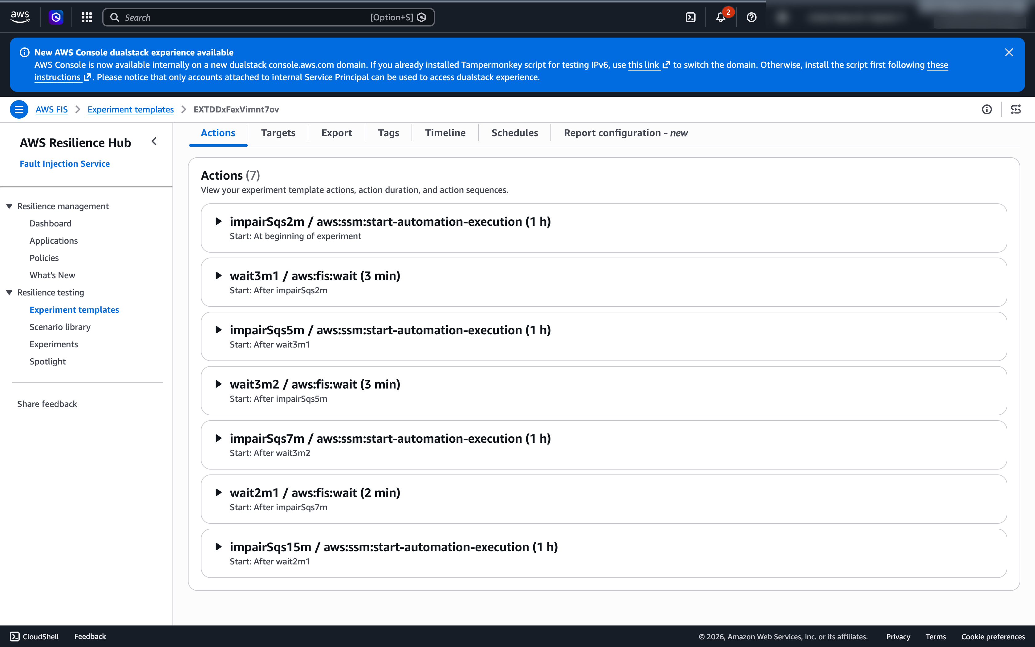
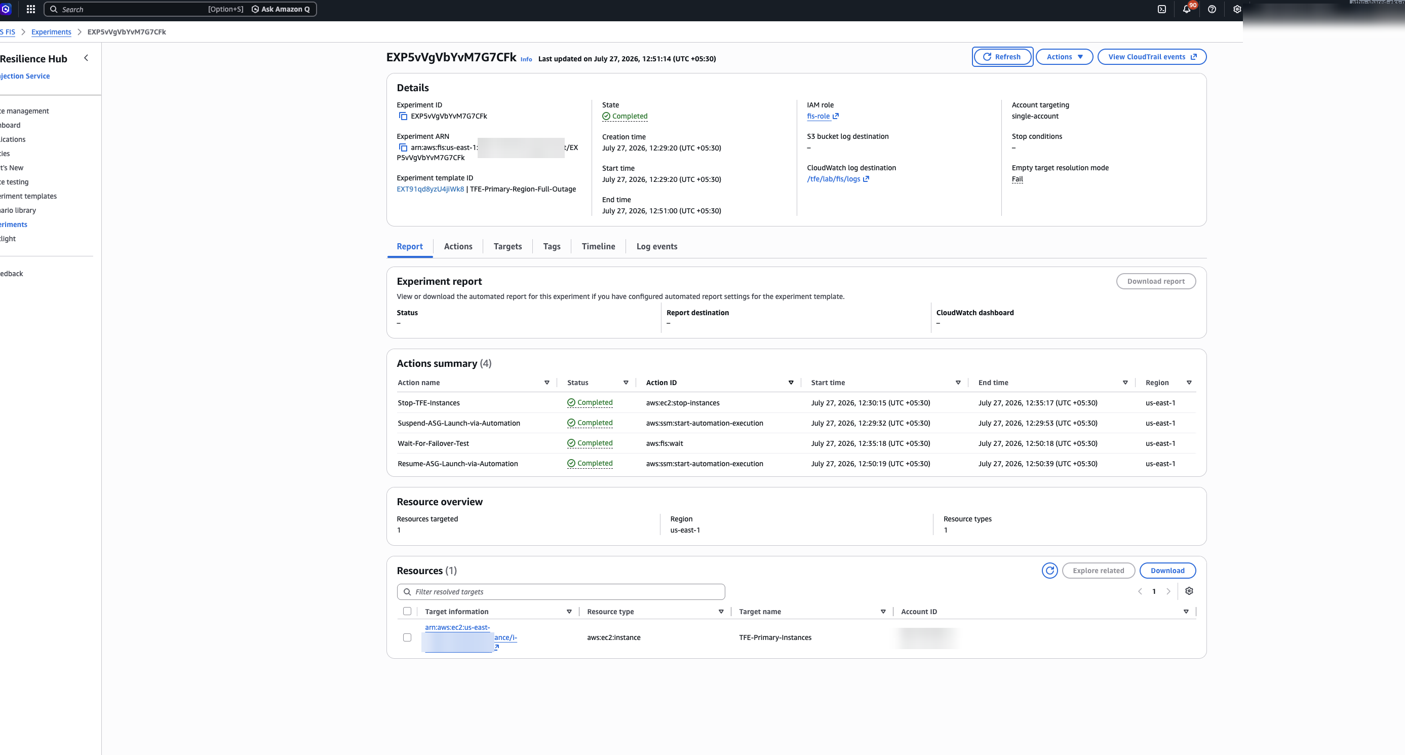
The FIS experiment template with four impairment actions of 2, 5, 7, and 15 minutes chained by recovery waits

Figure: The FIS experiment template: four impairment actions (2, 5, 7, and 15 minutes) chained with recovery waits between them.

Stop conditions. A stop condition halts the experiment automatically if a specified CloudWatch alarm fires, an essential control for an escalating experiment. A triggered stop condition also unwinds what it can: FIS cancels the run, and the automation’s onCancel step removes the deny, restoring access. That rollback is a property of this experiment’s design, not of stop conditions in general: an action like EC2 instance termination does not support rollback, so check each action’s rollback behavior before relying on a stop condition to help limit damage. The library template ships with "stopConditions": [{"source":"none"}], because the right alarm depends on health signals the template can’t assume.

Metric choice matters: alarming on a queue metric like ApproximateAgeOfOldestMessage or NumberOfMessagesSent would be incorrect, as those are supposed to move during impairment. So, the alarm would trip in the first 2-minute phase and abort the run before the longer phases surface anything interesting. You’d be alarming on the effect you’re injecting.

Instead, tie the stop condition to a signal that should stay healthy if your resilience mechanisms are working. This would reflect real customer impact. If that signal degrades more than you’ll tolerate (error rates that don’t recover within the 2 minutes your hypothesis allows), your resilience has already failed and continuing risks further customer impact. Some metrics to consider alarming on:

  • An application error rate or transaction-success metric (a custom CloudWatch metric your app emits, for example failed orders per minute), the most direct measure of customer impact and independent of the SQS metrics you’re perturbing.
  • Load balancer 5xx count or target response time (for example HTTPCode_Target_5XX_Count on an Application Load Balancer), a good proxy when you don’t yet emit a business metric.
  • DLQ depth: ApproximateNumberOfMessagesVisible on the dead-letter queue crossing a threshold, which signals messages are failing permanently rather than only backing up recoverably.

See Stop conditions for AWS FIS for more information.

Deriving the threshold from your hypothesis. The preceding hypothesis expects recovery within 2 minutes of access being restored. That number is also your alarm. If failed orders per minute is your customer-impact metric and its baseline is near zero, set the alarm to failed orders per minute > 10 for 2 consecutive 1-minute periods: long enough that a spike while the circuit breaker opens shouldn’t abort the run, short enough that failing to recover inside your hypothesis window stops it. Design the alarm for how the metric behaves during failure rather than for the test: when the circuit breaker opens, a low-volume custom metric might stop emitting data points entirely. Tighten it as you approach production.

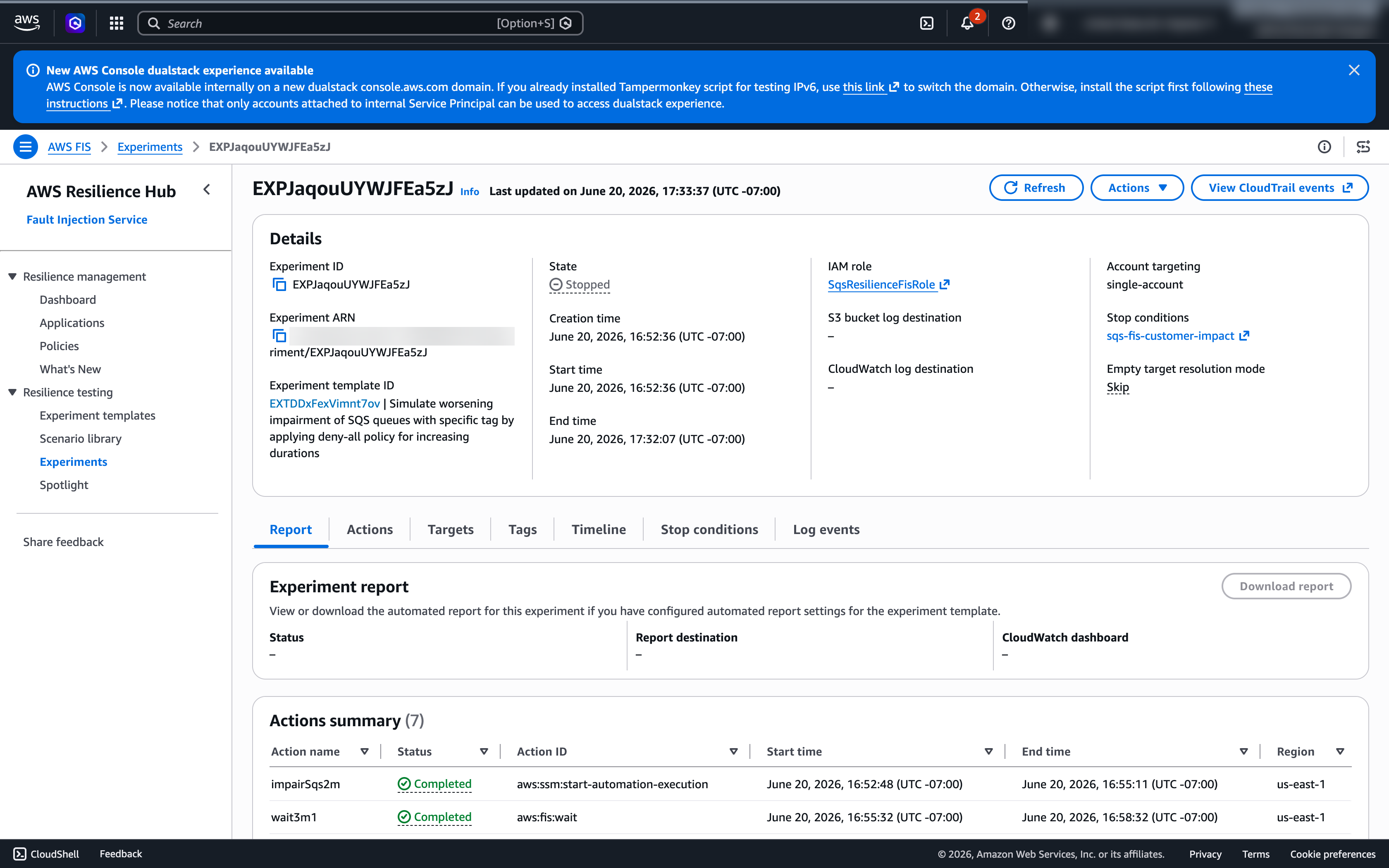
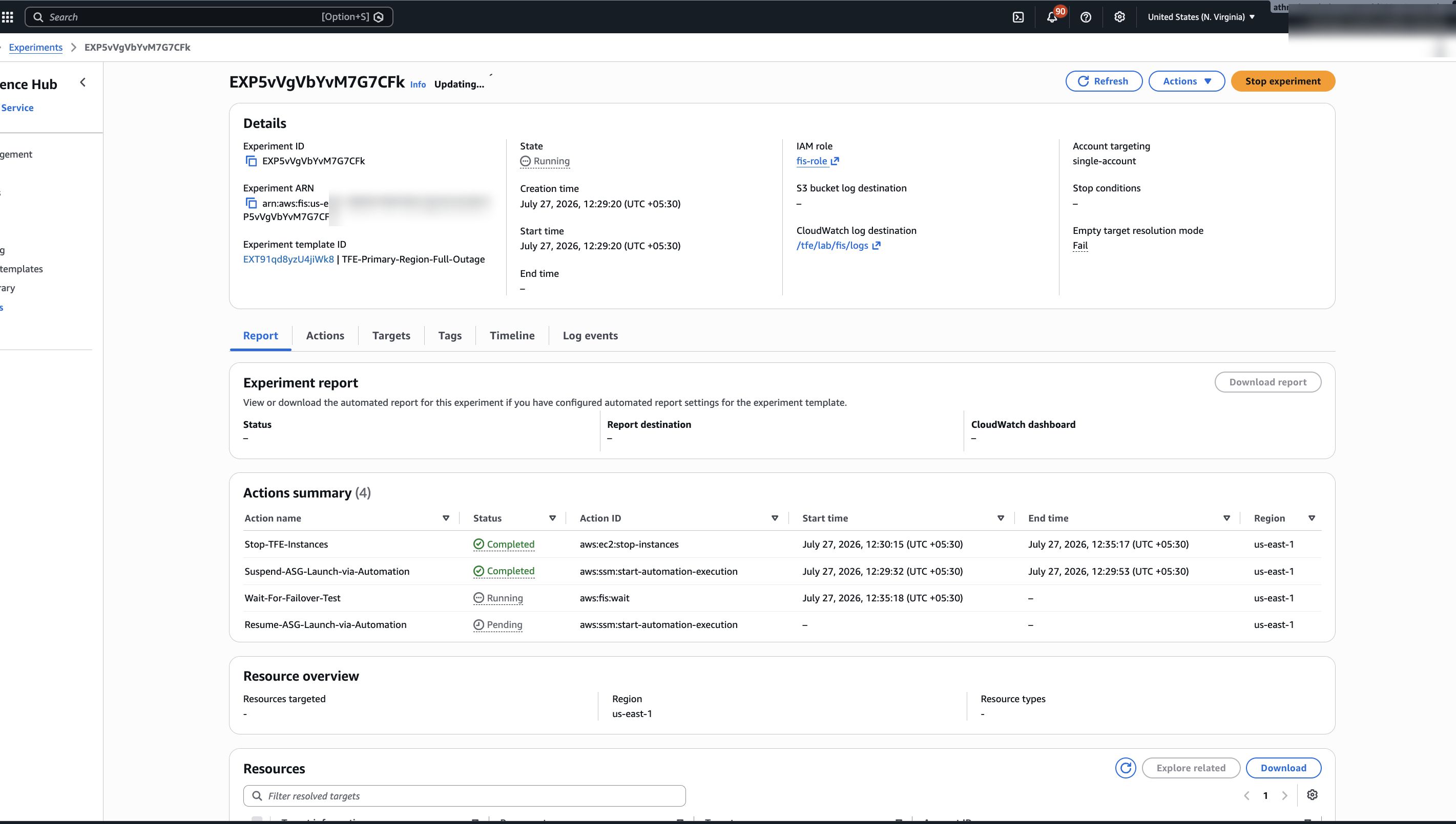
AWS FIS experiment in Stopped state after the customer-impact alarm breached and halted the run

Figure: When the customer-impact alarm breached, AWS FIS halted the experiment automatically (State: Stopped)

Running the experiment

To start the experiment with AWS FIS you can use the console or the AWS CLI:

aws fis start-experiment --experiment-template-id <YOUR_TEMPLATE_ID> --region <YOUR_REGION>

What to observe during impairment

During each phase, SQS operations return AccessDenied errors. Note what that does and doesn’t exercise: a 403 is non-retryable, so this experiment validates that your code recognizes it and stops, not your backoff path. To exercise retries and backoff, inject a retryable fault such as throttling or timeouts. The producer and the consumer fail differently, so watch them separately.

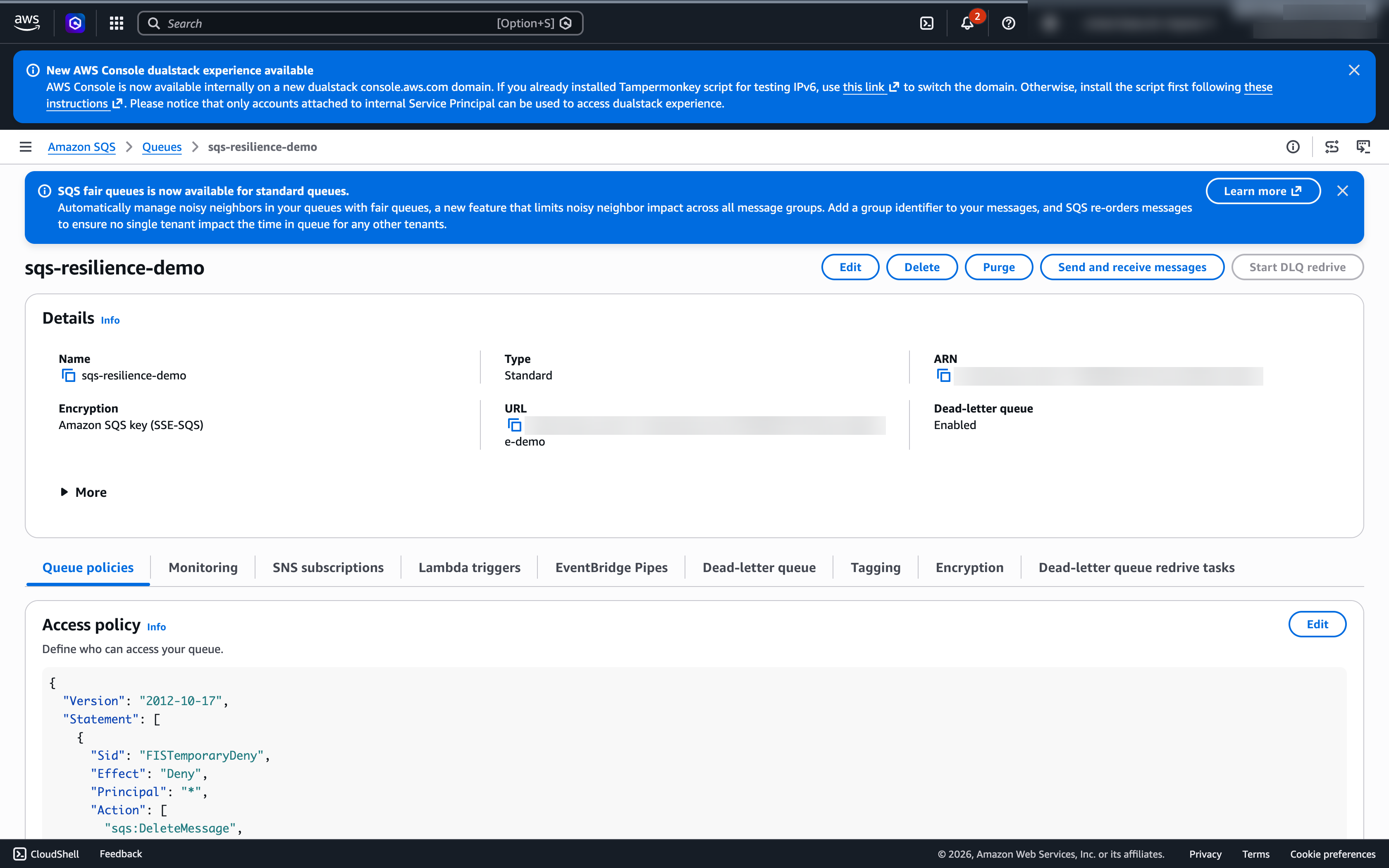
SQS queue access policy showing the scoped FISTemporaryDeny statement blocking SendMessage and ReceiveMessage

Figure: During impairment, the queue’s access policy carries the scoped FISTemporaryDeny statement; SendMessage and ReceiveMessage return AccessDenied while management actions still work.

Producer side (the component calling SendMessage):

Stage Healthy response Unhealthy response Signal to watch
First failed SendMessage Recognizes AccessDenied and fails fast Crashes, hangs, or blocks the calling thread NumberOfMessagesSent drops to ~0. Producer error rate rises
After 3 to 5 consecutive failures Circuit breaker opens. Sheds or buffers load Continues retrying indefinitely Circuit-breaker state metric. Producer CPU / threads / connections
Send gives up (non-retryable error, or retry budget exhausted) Fails fast and persists the payload to durable fallback storage, or alerts, does not silently drop Drops the message silently (permanent loss) Producer “failed send / dropped” counter. Fallback-store writes
Application state Stays responsive. Degrades gracefully Returns 500s to callers. Unbounded in-memory queueing Producer health checks, request latency
Resource usage Bounded by backoff and circuit breaker CPU/memory/connections climb (tight retry loops) Producer CPU, memory, connection-pool usage

Note: a producer that gives up on a send does not route anything to the DLQ.

Consumer side (the component calling ReceiveMessage / DeleteMessage):

Stage Healthy response Unhealthy response Signal to watch
First failed ReceiveMessage / DeleteMessage Backs off its poll loop rather than hammering. Any in-flight message returns to the queue after the visibility timeout Crashes or hangs the consumer loop NumberOfMessagesReceived / NumberOfMessagesDeleted drop
Backlog accumulates (consumers can’t drain) Backlog alarm fires. Scaling responds if keyed to queue depth (for example, backlog per worker) Backlog grows unbounded. Consumers idle-loop ApproximateNumberOfMessagesVisible stops draining (goes flat or climbs); ApproximateAgeOfOldestMessage climbs
Application state Idempotent processing. Safe to retry Duplicate side effects on redelivery Downstream idempotency / duplicate-write metrics
Resource usage Bounded by visibility timeout and backoff In-flight messages pile up. Consumer saturation ApproximateNumberOfMessagesNotVisible. Consumer CPU/memory

Don’t expect the DLQ to fill during impairment. Redrive is driven by maxReceiveCount: a message moves to the DLQ only after a consumer has received it that many times without deleting it. With ReceiveMessage denied, nothing is delivered, the receive count doesn’t increment, and nothing redrives. The DLQ depends on the very call that’s blocked, so it’s something to watch for during recovery, not during the outage.

Key CloudWatch metrics, and how to read them:

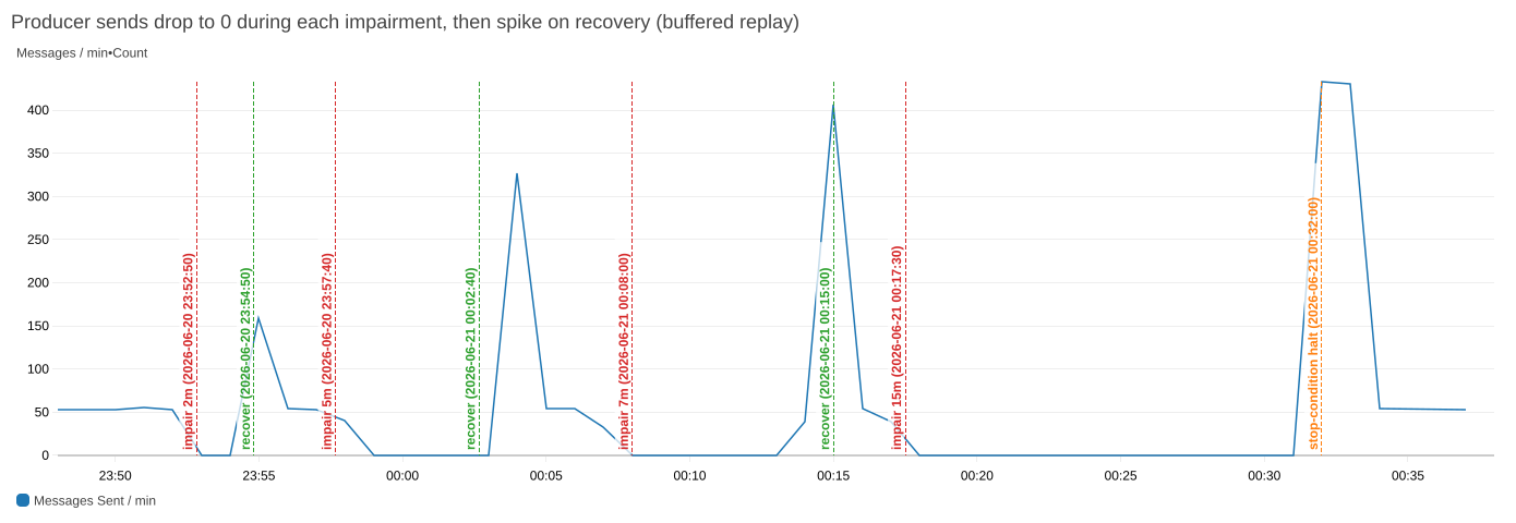
  • NumberOfMessagesSent: drops to zero when the deny policy takes effect and producers can no longer enqueue.
NumberOfMessagesSent dropping to zero during each impairment window and spiking on recovery, ending at the stop-condition halt

Figure: NumberOfMessagesSent drops to zero during every impairment window (red) and spikes on recovery (green) as buffered messages replay. The final phase ends at the stop-condition halt (orange).

  • ApproximateNumberOfMessagesVisible: the current backlog of messages available for retrieval. During impairment this often stops changing, a signal that tells you something is wrong precisely because it goes flat (nothing is being sent or drained).
  • ApproximateAgeOfOldestMessage: increases as unprocessed messages age, but only if the queue already held a message when the deny took effect. On an empty queue it won’t climb, which is why you read it alongside the visible-message count.
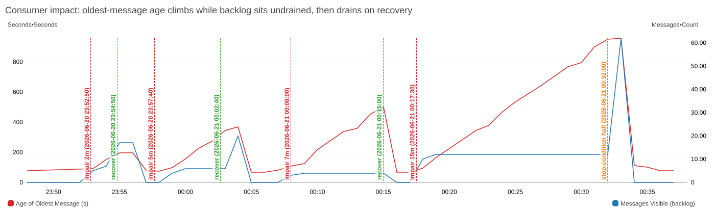
ApproximateAgeOfOldestMessage climbing while the visible backlog stays undrained during the 15-minute phase, then both collapsing on recovery

Figure: Consumer-side impact: ApproximateAgeOfOldestMessage climbs while the visible backlog sits undrained during the 15-minute phase, then both collapse the moment access is restored.

Application error rate: spikes initially, then stabilizes if circuit breakers engage.

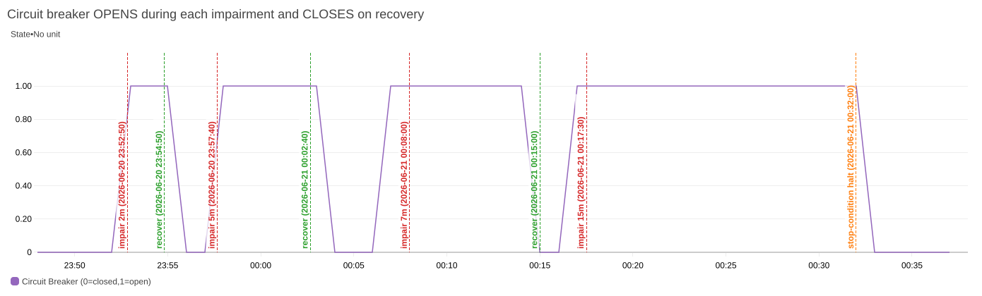
Producer circuit breaker opening within seconds of each impairment and closing on recovery as a square wave

Figure: The producer’s circuit breaker opens (1) within seconds of each impairment and closes (0) on recovery, a clean square wave that lags each fault window slightly because it opens only after a few sustained failures.

Count-based metrics (NumberOfMessagesSent/Received/Deleted) reflect system-level activity and can include retries and duplicates, so treat them as trend indicators rather than exact unique-message counts.

What to observe during recovery

When the deny policy is removed, the producer and consumer recover on different timelines.

Producer side:

What to observe Healthy response Unhealthy response
Send resumes NumberOfMessagesSent climbs back to baseline. Circuit breaker half-opens, then closes within ~30 seconds Circuit breaker stays open (stale failure state). Manual restart needed
Buffered / fallback payloads Replayed from durable fallback storage and re-sent idempotently Lost permanently (if silently dropped during impairment)
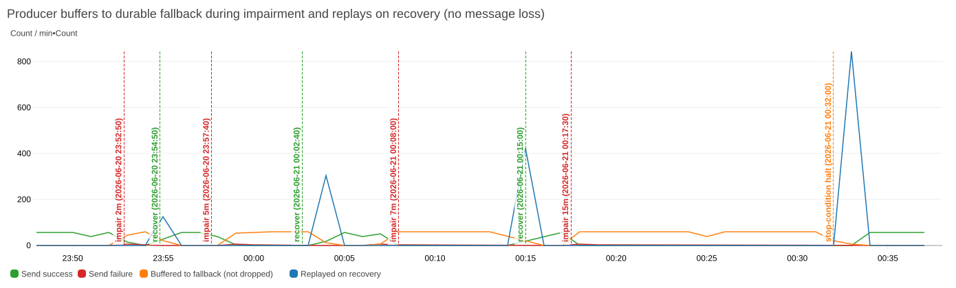
Producer buffering to durable fallback storage during impairment and replaying the buffer on recovery

Figure: The producer buffers to durable fallback storage during impairment (no dropped messages) and replays the buffer on recovery: send success, buffered writes, and replays over the run.

Consumer side:

What to observe Healthy response Unhealthy response
Receive / delete resumes NumberOfMessagesReceived / NumberOfMessagesDeleted recover Consumers stay wedged. No auto-recovery
Backlog burndown ApproximateNumberOfMessagesVisible drains steadily; ApproximateAgeOfOldestMessage falls Drain stalls: the rate spikes, then drops to zero and stays there (consumer overwhelmed or stuck)
DLQ contents Genuinely-poison messages redriven and reprocessed in controlled batches within the DLQ retention period Reprocessed all at once (overwhelming downstream), or left to age out of the DLQ and be deleted

Recovery is when the DLQ can move. A consumer overwhelmed by the accumulated backlog can re-fail messages and push some to the DLQ. If healthy messages land there, your maxReceiveCount is too low or your consumer isn’t keeping up.

Analyzing results

After the experiment completes, compare what happened against your hypothesis. Focus on these questions:

  • Did your circuit breakers activate? Measure from the first AccessDenied to when your application stopped attempting SQS operations. Over your target (typically 30 seconds) means your detection threshold is too high.
  • Did your system preserve messages? Reconcile attempted sends against messages processed after recovery, plus the DLQ and producer-side fallback storage. If the numbers don’t add up you have message loss, and the gap tells you which side lost them.
  • Are the recovered messages still worth processing? Preservation and relevance are different questions. After a long outage, some buffered sends and backlogged messages represent requests the client has already given up on, and processing them spends recovery capacity acting on stale intent. Compare each message’s timestamp to the current time as you consume it, and drop or sideline anything no longer actionable, deliberately rather than by letting it age out. See REL05-BP04: Fail fast and limit queues.
  • How did recovery behave? Look at ApproximateNumberOfMessagesVisible after each recovery period. A healthy system drains steadily. If the drain stalls (the rate spikes, then drops to zero and stays there), your consumer is overwhelmed or stuck.
  • Did longer disruptions reveal new failure modes? Compare the 2-minute phase against the 15-minute one. What tends to surface only under sustained failure:
    • Thread pool exhaustion from accumulated retry threads.
    • Memory pressure from buffered messages.
    • Connection pool starvation.
    • DLQ messages aging out: messages that sit in the DLQ longer than its retention period are deleted (see Best practices).

Results that match your hypothesis are evidence your resilience mechanisms work. Results that don’t are your work list.

Best practices

The sections below cover the resilience patterns that turn the gaps this experiment surfaces into fixes: retry logic, circuit breakers, dead-letter queues, and monitoring.

Retry logic with exponential backoff

Don’t retry everything. Retry only errors that might succeed on a repeat, such as throttling, timeouts, and transient 5xxs, and fail fast on non-retryable ones like the AccessDenied (403) this experiment injects. For the errors worth retrying, use exponential backoff with jitter: each failure increases the wait exponentially (1s, 2s, 4s, 8s, and so on) with a random offset that prevents producers who failed together from retrying together and spiking a recovering dependency.

The AWS SDKs have configurable retry behavior built in, so configure it rather than rolling your own. See Timeouts, retries, and backoff with jitter.

Circuit breakers

A circuit breaker stops attempting operations after a threshold of consecutive failures, then lets a single test call through after a recovery timeout. That saves resources on calls that are likely to fail and gives the dependency room to recover. Choose the open-state behavior deliberately: shedding or buffering load is safer than silently switching to an alternate path, because fallback paths are exercised only during failures and tend to fail with them. See Using load shedding to avoid overload and Avoiding fallback in distributed systems.

Dead letter queues

Configure a DLQ for every queue. It’s a consumer-side safety net for poison messages, not a producer overflow buffer. Set maxReceiveCount to the number of processing attempts that make sense for your workload (typically 3 to 5). Because redelivery is what feeds a DLQ, every consumer must tolerate seeing a message twice. See Making retries safe with idempotent APIs. For what a large post-recovery backlog can do, see Avoiding insurmountable queue backlogs.

A DLQ has no depth limit. The constraint is the retention period, after which SQS deletes the message (default 4 days, maximum 14). Set the DLQ’s retention longer than the source queue’s to provide more investigation time before messages are deleted. For standard queues, note that the retention clock runs from the original enqueue time and does not reset on the move to the DLQ, so time in the source queue counts against it. (FIFO queues do reset it.) After the experiment, confirm messages were preserved rather than aged out.

Monitoring strategy

For what to emit and at what granularity, see Instrumenting distributed systems for operational visibility. Build a CloudWatch dashboard combining these across the producer, the consumer, and the queue:

Queue-level metrics: NumberOfMessagesSent, NumberOfMessagesReceived, NumberOfMessagesDeleted, ApproximateNumberOfMessagesVisible, ApproximateNumberOfMessagesNotVisible, and ApproximateAgeOfOldestMessage, read as described in what to observe during impairment.

Application-level metrics:

  • Error rates by type (distinguish AccessDenied from other failures), tagged by producer vs. consumer.
  • Circuit breaker state changes (open / closed / half-open transitions).
  • DLQ message count.
  • End-to-end message processing latency.

Alarm on ApproximateAgeOfOldestMessage exceeding your SLA threshold as a production alert, but not as an experiment stop condition, since the metric is supposed to rise during impairment. Use a customer-impact signal there instead (see Stop conditions).

Clean up your environment

  • Verify the deny policy is gone. Check each queue’s access policy on the console or run aws sqs get-queue-attributes --queue-url <URL> --attribute-names Policy. If FISTemporaryDeny is still there, retrieve the policy, delete the statement, and reapply with aws sqs set-queue-attributes.
  • Process messages that landed in your DLQs during the experiment.
  • Review CloudWatch metrics to confirm your queues have returned to normal operation.
  • Document your findings: What matched your hypothesis, what didn’t, and what you’re fixing.

Expand your resilience testing

Once the basics hold, extend the experiment:

Partial failure: Impair only a subset of your queues to test whether your application handles mixed healthy/unhealthy dependencies.

Note: Don’t run two impairment experiments against the same queue concurrently. The automation reads the policy, modifies it, and writes it back. Concurrent runs can overwrite each other and leave a stale deny behind. Target distinct queues, or run them in sequence.

Consumer-side only: Block only ReceiveMessage and DeleteMessage while allowing SendMessage, to simulate a consumer outage while producers keep filling the queue (the most common real-world scenario).

Combine with other failures: Run the SQS experiment alongside EC2 instance termination or network latency injection to test compound failure scenarios.

Explore AWS Resilience Hub: Use AWS Resilience Hub to assess your application’s resilience posture and get recommendations for improvement.

Using FIS scenarios

A scenario is an AWS-authored template bundling the actions, targets, and duration for a recognizable event, so you start from a reviewed definition instead of assembling actions yourself. While AWS provides multiple scenarios in the library, here are two that are a good place to start.

AZ Availability: Power Interruption induces the symptoms of losing power in one Availability Zone: zonal EC2, ECS, and EKS compute stops, new launches in that AZ fail, and subnet connectivity is lost. It’s the sharper test of the queue-based decoupling this post exercises, because producers and consumers lose capacity while the queue itself is not targeted. You learn whether surviving consumers absorb the backlog, whether Auto Scaling replaces capacity in the remaining AZs rather than retrying in the impaired one, and whether the backlog drains inside your hypothesis window. It defaults to 30 minutes of impairment plus 30 of recovery, twice this post’s longest phase.

AZ: Application Slowdown introduces additional latency between resources within a single Availability Zone (AZ). This latency creates many of the symptoms of an application slowdown, a partial disruption, sometimes known as a gray failure. It adds latency to network flows between target resources. Network flows represent the traffic between computing resources: the data packets carrying requests, responses, and other communications between your servers, containers, and services. The scenario can help to validate observability setups, tune alarm thresholds, discover application sensitivity to slowdowns, and practice critical operational decisions like AZ evacuation.

Scenarios carry the same obligations: write the hypothesis first and set the stop condition on a customer-impact metric rather than one the scenario is designed to move. Your derived threshold works unchanged. Copy a scenario into your own template to narrow the targets or change the duration. See Working with the AWS FIS scenario library.

Conclusion

In this post, you learned how to discover what your application does when SQS operations fail, and whether you’d notice. Every gap between your hypothesis and the results is an opportunity to improve your system’s resilience and its observability.

Start with the 2-minute phase in a non-production environment. Fix what breaks. Then run the full sequence and keep running it as the application evolves. Each phase of growth brings failure modes you might only find under load.

For more information, see:


About the authors

Validating multi-Region DR for Terraform Enterprise with AWS FIS

Post Syndicated from Frenil Randeria original https://aws.amazon.com/blogs/architecture/validating-multi-region-dr-for-terraform-enterprise-with-aws-fis/

In October 2025, Athenahealth, a major North American Electronic Health Record (EHR) provider, discovered a gap. An AWS regional service event in us-east-1 made their single-Region HashiCorp Terraform Enterprise (TFE) deployment inaccessible to their developers. This post shares the architecture, the AWS Fault Injection Service (AWS FIS) validation approach, HashiCorp best practices, and lessons learned from the collaboration between AWS and HashiCorp. Together, these help increase resiliency and verify that the customer’s critical workloads remain active during regional service events.

Currently, Terraform Enterprise (TFE) deployments are only supported within a single AWS Region. This means that, for TFE customers without a well-tested DR plan, a regional service event can block your engineering teams from deploying, modifying, or recovering infrastructure. A multi-Region disaster recovery (DR) strategy addresses this risk. The architecture in this post is a customer-operated DR pattern: HashiCorp supports TFE within a single Region and the HVD module targets single-Region deployments, so the multi-Region failover described here is designed, operated, and tested by the customer rather than provided as a supported product configuration. That strategy only works if you validate your regional failover workflow before you need it. Reacting during an event that impairs your primary Region costs developer productivity and business continuity. AWS FIS exposes hidden dependencies and configuration issues by injecting real failures into your AWS environment.

The following sections walk you through how to design three-phase AWS FIS experiments for TFE, expose hidden dependencies in failover automation, and validate both failover and failback for a multi-Region TFE deployment. You can help prevent extended downtime that impacts your infrastructure deployment capabilities and achieve 12-14 minute recovery times.

Prerequisites

To follow the validation approach in this post, you should have the following:

Starting architecture

If you’re running TFE in a single Region within AWS, this section describes the starting point. Athenahealth’s deployment used HashiCorp’s Terraform Enterprise Validated Design (HVD) module with the following components:

  • Amazon Elastic Compute Cloud (Amazon EC2) instances running TFE application servers.

  • Amazon Aurora PostgreSQL-Compatible Edition for application state.

  • Amazon Simple Storage Service (Amazon S3) for Terraform workspace state files.

Athenahealth hosted these components in the us-east-1 Region. The deployment provided Availability Zone-level resilience but lacked regional failover capabilities. The October 2025 event highlighted what was missing: no cross-Region database replication, no secondary Region compute capacity, no Terraform state file backup outside us-east-1, and DNS pointing exclusively to the primary Region.

Following the October 2025 event, Athenahealth engaged both their AWS and HashiCorp account teams for guidance on protecting not only TFE, but other critical workloads as well. The three organizations worked as a single team to design and implement a multi-Region DR strategy for the TFE environment. By combining the AWS Well-Architected Framework guidance regarding operational excellence and reliability, along with HashiCorp’s best practices regarding DR strategies using Terraform, the team came up with the multi-Region architecture (Figure 1) that would replace the customer’s current single-Region deployment.

Multi-Region DR solution

With an active-passive multi-Region design across us-east-1 (primary) and us-west-2 (DR), Athenahealth achieved a 12-14 minute Recovery Time Objective (RTO) and less than 1 minute Recovery Point Objective (RPO). In the AWS disaster recovery taxonomy, this is a pilot light strategy: data replicates continuously to the DR Region while compute stays at zero. A warm standby variant (DR minimum capacity of 1) trades higher cost for faster RTO. This section covers the architecture components that make this possible and the four-step failover process you can follow during a regional service event.

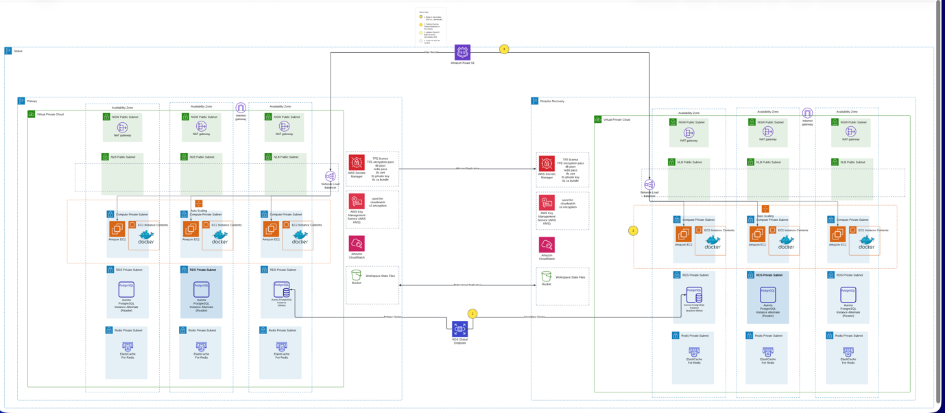
Multi-Region active-passive DR architecture for Terraform Enterprise with bidirectional S3 replication and a Route 53 health check.

Figure 1: Multi-Region active-passive DR architecture for Terraform Enterprise on AWS. Note the bidirectional S3 replication arrows between Regions and the Amazon Route 53 health check that determines the active Region.

The example Terraform code used to configure and manage the core architecture components, along with the failover process can be found in this sample GitHub repository. You can use this code to test a similar pattern for your TFE workload.

Core architecture components

You can route traffic to the active Region with Amazon Route 53 DNS alias records pointing to an Elastic Load Balancing (ELB) Network Load Balancer. Alias records for ELB targets use a 60-second time-to-live (TTL), which limits how long DNS resolvers cache the record. Clients begin resolving to the DR Region within about a minute of failover rather than waiting for longer cached entries to expire.

In each Region, an Amazon Virtual Private Cloud (Amazon VPC) spans three Availability Zones, and Amazon EC2 Auto Scaling groups manage the TFE instances. To help minimize cost, Athenahealth scaled DR Region compute to zero during normal operations by setting the Auto Scaling group minimum capacity to 0.

For cross-Region database replication, Athenahealth uses Aurora PostgreSQL-Compatible global databases, which provide sub-second replication lag and managed failover. The primary cluster runs one writer and two readers across three Availability Zones. The secondary cluster maintains an inactive writer that’s ready for promotion.

You can replicate Terraform workspace state files bidirectionally between primary and DR Amazon S3 buckets with S3 cross-Region replication. This design supports failback without data resynchronization.

AWS Secrets Manager and AWS Key Management Service (AWS KMS) provide cross-Region credential and encryption key management. Two TFE-specific dependencies deserve attention when you design for multi-Region. First, the TFE encryption password protects the internal Vault unseal key and root token. DR instances configured with a different value cannot start or decrypt existing data, so verify that this secret is replicated to your DR Region and referenced by your DR launch configuration. Second, if you run TFE in Active/Active mode, external Redis holds the job queue and cache. Account for a Redis equivalent in the DR Region and decide what in-flight job loss is acceptable at failover. Amazon CloudWatch alarms in each Region monitor the TFE instances, Auto Scaling groups, and Aurora clusters in that Region. Detection of a primary Region impairment does not depend on the primary Region itself: the Amazon Route 53 health check shown in Figure 1 probes the TFE endpoint from a globally distributed checker fleet, and alerts publish through Amazon Simple Notification Service (Amazon SNS) topics in both Regions.

Failover process

The architecture uses a four-step failover sequence:

1. Activate DR Auto Scaling group (2-5 minutes). Scale from 0 to 1 instance and validate health checks. TFE exposes a health check endpoint (/_health_check) that returns a 200 OK response when the application is running. The Network Load Balancer target group and the Route 53 health check probe this endpoint to determine instance health.

2. Promote Aurora PostgreSQL-Compatible global database (~1 minute). Promote the DR writer. Complete this step before DNS failover shifts traffic to the DR Region, to help prevent both Regions from accepting writes simultaneously (known as a split-brain scenario in distributed databases).

3. Confirm Amazon Route 53 DNS failover (~60 seconds). The pre-configured Route 53 failover routing policy detects the unhealthy primary endpoint and routes traffic to the DR Region’s Network Load Balancer. This happens in the Route 53 data plane, with no record modifications at failover time.

[Important: Your failover process should not depend on control plane API calls during an event. Modifying Route 53 records to perform failover is a documented anti-pattern because the Route 53 control plane operates from a single Region. Athenahealth avoided this dependency with pre-configured health check-based failover routing. For manually initiated Region switches through a highly available data plane, consider Amazon Application Recovery Controller (ARC) Region switch, which Athenahealth plans to evaluate in a future phase.]

4. Scale out for production load (5-10 minutes). Increase Auto Scaling group capacity while monitoring Amazon CloudWatch.

Note: Run failover scripts from outside the primary Region—for example, from the DR Region, a separate management Region, or a CI/CD system that is not dependent on the primary Region. If your failover automation runs in the primary Region, it might be unreachable during the event you are trying to recover from.

The ordering between Aurora promotion and traffic shift is enforced procedurally rather than by an automated control. The DR Auto Scaling group runs at zero capacity during normal operations, so the DR endpoint cannot pass health checks until an operator executes the runbook, and the runbook sequences promotion ahead of scaling for traffic. For an orchestrated Region switch with explicit sequencing controls, consider Amazon Application Recovery Controller Region switch, which Athenahealth plans to evaluate in a future phase.

Total failover execution time: 12-14 minutes, meeting the established RTO.

Validating with AWS Fault Injection Service

With the multi-Region architecture now in place, we still needed to confirm it would work under real failure conditions. This is where AWS FIS was introduced into the DR workflow. AWS FIS injects controlled failures into your AWS environment that can be used to measure actual recovery times and catch configuration issues before an actual disruption. The following three phases show how Athenahealth validated their architecture, and you can apply the same approach to your TFE deployment as well.

Progressive experiment approach

Rather than testing full regional failover immediately, the team validated resilience in three progressive phases starting with individual compute failures, then database failover, and finally simulated S3 connectivity loss. Each phase built confidence in a specific layer of the architecture before combining them, and each surfaced issues that manual review had missed.

Phase A: Amazon EC2 and Auto Scaling group failure injection

Athenahealth hypothesized that if TFE instances were stopped or Amazon EC2 capacity became unavailable, the Auto Scaling group would launch replacement instances within five minutes without manual intervention. To test this, they ran the following AWS FIS actions: aws:ec2:stop-instances, aws:ec2:asg-insufficient-instance-capacity-error, and Auto Scaling group suspend and resume operations. You can use these same actions to validate your own Auto Scaling group recovery behavior.

The results confirmed the hypothesis. The Auto Scaling group detected failed instances and launched replacements within 2-3 minutes. Network Load Balancer health checks removed failed instances from rotation within 30 seconds.

These experiments also revealed an outdated Amazon Machine Image (AMI) reference in the DR Region’s Auto Scaling group launch template. Athenahealth builds custom AMIs and copies them to the DR Region, but the DR launch template still referenced an older version. This configuration drift only surfaced when AWS FIS forced the Auto Scaling group to launch new instances. If you’re running similar experiments, check the launch template AMI references in both Regions as part of your validation.

AWS FIS console experiments list showing one experiment in the Running state.

Figure 2. FIS experiments list showing experiment EXP5vVgVbYvM7G7CFk in Running state, created July 27, 2026 at 12:29:20 IST.

AWS FIS experiment details page showing the Suspend-ASG action completed and Stop-TFE-Instances running.

Figure 3. FIS experiment details showing template TFE-Primary-Region-Full-Outage, CloudWatch log destination /tfe/lab/fis/logs, Suspend-ASG completed, and Stop-TFE-Instances running.

Amazon EC2 console showing the primary instance in us-east-1 in the stopped state.

Figure 4. Primary EC2 instance in us-east-1 stopped after the FIS stop-instances action.

AWS FIS action summary showing Stop-TFE-Instances completed and Wait-For-Failover-Test running.

Figure 5. FIS action summary showing Stop-TFE-Instances completed at 12:35:17 IST and Wait-For-Failover-Test running.

AWS FIS experiment running during the wait window, with the stop action completed and the resume action pending.

Figure 6. FIS experiment still running during the wait window, with stop action completed and resume action pending.

AWS FIS experiment completed with all four actions showing completed, including Resume-ASG-Launch-via-Automation.

Figure 7. FIS experiment completed at 12:51:00 IST. All four actions show completed, including Resume-ASG-Launch-via-Automation.

Phase B: Aurora PostgreSQL-Compatible database cluster failover

Athenahealth hypothesized that if the Aurora PostgreSQL-Compatible global database cluster failed over, TFE would resume writes within one minute without manual intervention. To test this, they ran the aws:rds:failover-db-cluster AWS FIS action. The results confirmed the hypothesis for the database layer. Aurora promoted the secondary cluster’s writer in 58 seconds. During the promotion, TFE experienced approximately 15 seconds of write unavailability.

The Amazon Relational Database Service (Amazon RDS) Global Endpoint automatically redirected connections to the new writer. Athenahealth also discovered that the application layer did not meet the hypothesis. TFE connection pooling settings caused extended reconnection delays.

They reduced the connection pool timeout from 60 seconds to 10 seconds, which improved recovery time significantly. If you’re running TFE with Aurora PostgreSQL-Compatible, review your connection pool settings as part of your AWS FIS validation.

Note that this experiment exercised the coordinated failover path of Aurora, which requires the primary Region to be reachable to synchronize before promotion. During an actual event impairing the primary Region, you would instead use Aurora Global Database managed failover (the failover-global-cluster command with the --allow-data-loss option) or a manual detach-and-promote. These paths do not wait for replication to synchronize, so promotion timing differs and the RPO is bounded by the replication lag at the time of the event rather than zero. Treat the 58-second promotion and sub-second lag measured here as coordinated-path results, and plan unplanned-path expectations using the Aurora Global Database disaster recovery documentation.

Phase C: Amazon S3 connectivity disruption

Athenahealth hypothesized that if TFE lost connectivity to Amazon S3 in the primary Region, the DR Region bucket would hold current replicated state files without data loss. Testing this required a workaround, because AWS FIS doesn’t provide a direct action to disrupt Amazon S3 access. You can use the aws:network:disrupt-connectivity action instead to inject network ACL rules that block S3 traffic at the subnet level.

The aws:network:disrupt-connectivity action targets subnets, not S3 buckets directly. AWS FIS injects network ACL rules on compute private subnets, which blocks egress traffic to S3 service endpoints and simulates Regional S3 disruption for TFE instances in those subnets.

This experiment validates the S3 consumer, meaning TFE losing access to S3. It does not disrupt S3 cross-Region replication, because service-side replication between buckets does not traverse your subnet network ACLs. To test delayed or paused replication between Regions, use the Cross-Region: Connectivity scenario described in Next steps. Note that this approach assumes your TFE instances reach S3 over an in-VPC path, such as a gateway VPC endpoint, so the injected network ACL rules sit on the egress path to S3.

To configure this AWS FIS experiment, use the following template. Replace <your-tfe-compute-private-subnet-prefix> with your actual subnet name prefix, which you can find in the Amazon VPC console under Subnets.

{
    "actions": {
        "DisruptS3Connectivity": {
            "actionId": "aws:network:disrupt-connectivity",
            "parameters": {
                "duration": "PT10M",
                "scope": "all"
            },
            "targets": {
                "Subnets": "TFE-Compute-Private-Subnets"
            }
        }
    },
    "targets": {
        "TFE-Compute-Private-Subnets": {
            "resourceType": "aws:ec2:subnet",
            "resourceTags": {
                "Name": "<your-tfe-compute-private-subnet-prefix>-*"
            },
            "selectionMode": "ALL"
        }
    }
}

The results confirmed the hypothesis for data durability. TFE detected S3 connectivity loss within 5 seconds. The DR Region S3 bucket contained replicated state files with less than 30 seconds of replication lag, and bidirectional replication prevented state file loss. The experiment also exposed a failure mode Athenahealth had not anticipated: the state file dependency issue detailed in the following section.

Combined experiment: primary Region impairment

After validating each layer individually, the team combined the faults into a single AWS FIS experiment template (shown in Figures 2-7). The experiment suspends the primary Region Auto Scaling group, stops the TFE instances, holds the faults in place during a wait window while the team executed the four-step failover runbook, and then resumes the Auto Scaling group. This end-to-end run validated the complete failover process under simultaneous compute impairment. The combined run surfaced no new failure modes beyond those found in the individual phases, which was itself the confirmation the team wanted.

Measuring recovery times

Across the three AWS FIS experiment phases, Amazon CloudWatch measured the following recovery times:

  • Amazon EC2 failure recovery: 2-3 minutes (automated Auto Scaling group replacement)

  • Aurora PostgreSQL-Compatible failover: 1-2 minutes (managed promotion)

  • Failover execution time: 12-14 minutes (operator-triggered four-step process)

  • Aurora replication lag: less than 1 second (99th percentile)

  • S3 replication lag: less than 30 seconds (99th percentile)

  • Data loss during failover: 0 bytes (across each experiment)

[Note: These measurements reflect controlled testing conditions. Aurora Global Database and S3 cross-Region replication are both asynchronous. During an actual event, writes committed within the replication lag window (sub-second for Aurora, up to 30 seconds for S3) may not yet be available in the DR Region. Plan for near-zero rather than zero data loss when setting RPO expectations.]

  • Failback RTO: approximately 20 minutes (including approximately 5 minutes for Aurora PostgreSQL-Compatible global database re-establishment)

The 12-14 minutes measure failover execution time, from the operator triggering the runbook to full recovery. End-to-end recovery from event onset also includes detection time and the decision to fail over, so plan for a larger overall RTO.

Lesson learned: the state file dependency pitfall

Athenahealth first identified this risk during production failover and failback testing: their automation scripts depended on Terraform S3 state file outputs from both Regions. Subsequent AWS FIS experiments (Phase C) confirmed the severity. When S3 access is lost, those scripts fail entirely.

How the dependency breaks failover

Athenahealth’s failover and failback scripts automate the four-step process described earlier: scaling the Auto Scaling group in the target Region, promoting the Aurora global database writer, and verifying application health. An operator triggers them as part of the manual failover runbook, and they run from outside the primary Region. In their original form, the scripts retrieved infrastructure identifiers such as the Amazon RDS global cluster ID and Auto Scaling group name from state files stored in Amazon S3:

# Failover script excerpt (problematic approach)
# Retrieve RDS Global Cluster ID from primary Region state file
RDS_GLOBAL_CLUSTER_ID=$(terraform output \
    -state=s3://<primary-region-bucket>/terraform.tfstate \
    rds_global_cluster_id)

# Retrieve DR Auto Scaling group name from primary Region state file
DR_ASG_NAME=$(terraform output \
    -state=s3://<primary-region-bucket>/terraform.tfstate \
    dr_asg_name)

# Run Aurora failover
aws rds failover-global-cluster \
    --global-cluster-identifier $RDS_GLOBAL_CLUSTER_ID \
    --region us-west-2

For an unplanned Regional impairment, add the --allow-data-loss option to this command to perform a managed failover instead of a switchover, because a switchover requires the primary Region to be healthy.

During a Regional service impairment, the primary Region’s S3 state file may be unreachable. The same applies in reverse during failback. The failover script tries to read the state file, S3 times out, and the script stops. This creates a circular dependency: you can’t run the failover without access to the infrastructure you’re trying to recover from.

How to remove the dependency

The underlying principle is to remove every recovery dependency on the Region you are recovering from. Failover automation must not read configuration from the control plane or data plane of the impaired Region. Athenahealth implemented this principle by hardcoding infrastructure identifiers directly in their failover scripts. You can obtain these values from your Terraform outputs during normal operations:

# Failover script excerpt (resilient approach)
# Infrastructure identifiers hardcoded, not from dynamic lookups
RDS_GLOBAL_CLUSTER_ID="<your-tfe-global-cluster>"
DR_ASG_NAME="<your-tfe-dr-asg-us-west-2>"
ROUTE53_HOSTED_ZONE_ID="<your-hosted-zone-id>"

# Run Aurora failover with no state file dependency
aws rds failover-global-cluster \
    --global-cluster-identifier $RDS_GLOBAL_CLUSTER_ID \
    --region us-west-2

The trade-off is maintenance: hardcoded values require manual updates when infrastructure changes. Athenahealth addressed this with a CI/CD pipeline that compares hardcoded values against Terraform outputs and alerts on drift.

Hardcoding is one implementation of the principle. A Region-independent configuration source outside the primary Region achieves the same resilience with less drift risk, such as an AWS Systems Manager Parameter Store parameter replicated across Regions, an Amazon DynamoDB global table, or values committed to the repository that holds your failover scripts.

Testing failback

The state file dependency affected both failover and failback. Athenahealth validated failback by running full failover to DR, operating there for 30 minutes, then returning to primary. Bidirectional S3 replication prevented state file loss.

Collaboration model

If you’re planning a multi-Region DR project for TFE, consider a cross-functional approach. Athenahealth’s five-month engagement combined AWS resilience and AWS FIS expertise, HashiCorp TFE architecture knowledge, Terraform DR best practices, and HVD modules. This combination helped the customer reach production-validated DR faster than working independently. You can engage AWS Support or AWS Professional Services for similar guidance.

Conclusion

You can maintain infrastructure deployment capabilities during events that impact a single Region with a validated multi-Region DR architecture for TFE. This architecture achieved a validated RTO of 12-14 minutes and an RPO of less than 1 minute.

Multi-Region DR is not the right choice for every TFE deployment. Athenahealth chose this approach because TFE manages infrastructure for critical healthcare workloads. The October 2025 event showed that losing the ability to deploy during a regional event was a risk the business could not accept. Costs vary based on your configuration, but Athenahealth observed costs approximately 30-40% higher than their single-Region deployment, primarily from Aurora PostgreSQL-Compatible global database replication and S3 cross-Region replication. Weigh this cost against your own RTO and RPO requirements. For less critical workloads, a single-Region deployment with regular backups and a tested restore process may meet your needs.

Key takeaways

  1. Give your infrastructure as code (IaC) tools the same resilience as production workloads. When your TFE deployment becomes unavailable during a Regional service event, you can’t deploy fixes or recover infrastructure.

  2. Validate DR with controlled failure injection. AWS FIS experiments simulating real S3 connectivity loss exposed the state file circular dependency, a failure mode that only surfaces under actual disruption conditions.

  3. Remove recovery dependencies on the Region you are recovering from. Dynamic lookups from state files tie failover to the infrastructure being recovered. Hardcoded identifiers or a Region-independent configuration source both work. Use drift detection to keep values current.

  4. Test failback, not only failover. Without failback validation, you risk getting stuck in the DR Region or causing data loss when returning to primary.

  5. Use subnet-level network disruption to simulate S3 connectivity disruption. The aws:network:disrupt-connectivity action targeting compute subnets simulates Regional S3 connectivity loss, which is the recommended approach because AWS FIS doesn’t offer a direct S3 disruption action.

Next steps

You can implement this solution in your environment with the following steps:

1. Run Phase A AWS FIS experiments on non-production TFE instances to validate Auto Scaling group recovery.

2. Review the HashiCorp’s Terraform Enterprise Validated Design module and DR guidance.

3. Establish your RTO and RPO targets before designing your Aurora replication strategy.

4. Create your first AWS FIS experiment to validate your DR architecture.

After you validate these three phases, extend your testing with additional AWS FIS scenarios. The AZ Availability: Power Interruption scenario validates recovery from the loss of an Availability Zone. The Cross-Region: Connectivity scenario simulates disrupted network connectivity between Regions, including paused S3 replication, which would delay state file replication to your DR Region.

If you need help designing or validating a multi-Region DR strategy, contact AWS Support or AWS Professional Services.

Cleanup

If you deploy this architecture for testing, delete the following resources in both Regions to avoid ongoing charges:

  • Aurora PostgreSQL-Compatible global database clusters.

  • Amazon S3 buckets with cross-Region replication.

  • Amazon EC2 instances in the DR Region Auto Scaling group.

If you used the sample GitHub repo to set up a test multi-Region TFE environment, verify that you also run terraform destroy to avoid any additional charges.

Resources:


About the authors

Architecting SASE solutions using AWS Local Zones

Post Syndicated from Lakshmi VP original https://aws.amazon.com/blogs/compute/architecting-sase-solutions-using-aws-local-zones/

Organizations with geographically distributed workforces face a critical challenge: providing secure, low-latency access to applications without routing all traffic through centralized data centers. Traditional hub-and-spoke network architectures create latency bottlenecks and degrade user experience, forcing a trade-off between security and performance.

This post explores how you can use AWS Local Zones and Secure Access Service Edge (SASE) solutions to eliminate that trade-off. You will learn key design principles, implementation strategies, and technical considerations for deploying SASE solutions at the edge. We’ve seen that understanding your user locations and traffic volumes up front helps you make effective design decisions.

Key challenges for deploying SASE solutions

SASE solutions require virtual security appliances such as firewalls, secure web gateways, and zero trust network access (ZTNA) connectors. You deploy these appliances close to end users so that traffic inspection does not add latency to the user experience. With AWS Local Zones, you can deploy these virtual security appliances from AWS Marketplace closer to end users.

When you architect SASE solutions using Local Zones, you need to address several key technical challenges. Latency requirements: When end users are far away from an AWS Region, applications requiring security inspection experience significant latency overhead that affects overall performance and user experience. Geographic coverage: In some cases, workforces are spread across distributed locations far from an AWS Region. You need solutions that deliver consistent service quality and security capabilities to users across your covered locations.

Hybrid connectivity: Many applications maintain dependencies on on-premises data centers in areas far away from an AWS Region. Design traffic routing carefully to avoid unnecessary network paths and reduce traffic hairpinning or network flapping. Security consistency: Implement uniform security controls across all distributed locations while maintaining performance. This requires consideration of service placement and routing architecture.

Before looking at the SASE-specific design, it helps to understand what Local Zones provide. The following diagram shows how Local Zones extend AWS infrastructure from the Region out to metropolitan areas closer to end users.

High-level AWS infrastructure diagram showing how Local Zones bring compute closer to users

Figure 1: High-level AWS infrastructure diagram showing how Local Zones bring compute closer to users

As the diagram shows, Local Zones place compute closer to end users. This especially benefits those far from an AWS Region.

Prerequisites

To follow the guidance in this post, you should be familiar with:

Architecture considerations

When you design SASE solutions with Local Zones, you can follow several key best practices across infrastructure, control plane, and traffic management.

Infrastructure deployment

At the infrastructure level, focus on deploying virtual security appliances to optimize coverage and performance. Start by selecting and configuring Amazon EC2 instances optimized for maximum network throughput. Choose instance families that provide the compute and networking capabilities required for traffic inspection workloads, with enhanced networking enabled for high packets-per-second performance.

Design a scalable cluster management strategy that adapts to varying workload demands while maintaining consistent security posture. As you deploy these clusters, establish proper multi-tenant isolation to maintain security boundaries between different organizational units, keeping user resources separate from management infrastructure.

Control plane architecture

The SASE control plane requires particular attention in distributed deployments. Deploy control components in an AWS Region to manage security appliances across all Local Zone locations. This provides a single point of policy distribution and configuration management. From this centralized vantage point, you can implement policy management that maintains consistency in security enforcement across all locations.

Visibility matters as much as policy enforcement. Implement standardized telemetry collection mechanisms, such as Amazon CloudWatch metrics and logs, across all locations so you can maintain observability and resolve issues proactively. As your deployment grows, automate configuration deployment using infrastructure as code (IaC) tools such as AWS CloudFormation or Terraform. This keeps deployment consistent across all edge locations and reduces manual errors when operating at scale.

Traffic management

Traffic management completes the architecture of a well-designed SASE solution. Use Amazon Route 53 with geoproximity routing and health checks to direct users to the nearest security inspection point, minimizing inspection latency. If an appliance fails, Route 53 automatically reroutes traffic to the next-nearest Local Zone. For critical deployments, maintain standby capacity in the parent Region as a fallback.

Deploy VPN endpoints in Local Zones closest to your user populations to reduce connection latency for remote users while maintaining high availability through health-checked failover across multiple locations. Plan your Internet Service Provider (ISP) connectivity for redundancy and performance requirements across different geographical locations, and implement geographic load-balancing mechanisms to distribute traffic efficiently across available resources.

You also need to consider the egress path, which is how traffic exits after inspection. For internet-bound traffic, use the Local Zone’s direct internet egress to avoid routing back through the parent Region. For traffic destined to applications in an AWS Region, traffic traverses the AWS private network between the Local Zone and its parent Region. Validate egress paths using VPC Flow Logs and traceroute to confirm traffic is not taking unintended hops.

The following diagram shows how the Local Zones architecture applies to a SASE use case, routing user traffic to a nearby Local Zone for inspection.

Remote users and branch offices routing traffic to virtual network firewalls in the nearest Local Zone, with control nodes in the parent AWS Region

Figure 2: Enterprise SASE deployment using virtual network firewalls across Local Zones to secure remote user and branch office access

As the diagram shows, remote users and branch offices connect to virtual network firewalls running in the Local Zone closest to them. Each Local Zone performs local traffic inspection that reduces latency for the SASE use case. The control nodes in the parent AWS Region manage policy and configuration across all locations.

Reference implementation approach

This section outlines the key phases for implementing a SASE solution across AWS Local Zones, from initial planning through validation.

Phase 1: Plan your deployment

Begin by mapping your user locations and latency expectations to identify which Local Zones are closest to your user populations, and determine which applications require local security inspection. With this map in hand, calculate capacity needs per location based on expected traffic volumes and security inspection requirements. Then define the specific inspection capabilities you need at each location, whether that is firewall, secure web gateway, ZTNA, or a combination.

One key design decision at this stage is whether to route all user traffic through the Local Zone appliance (full tunnel) or only corporate-bound traffic (split tunnel). Full tunnel provides complete traffic visibility but requires higher instance throughput. You can validate your choice by using VPC Flow Logs and CloudWatch network metrics to measure actual traffic volume per user during a pilot deployment.

Phase 2: Configure networking infrastructure

With your plan in place, enable the target Local Zones in your AWS account and create a VPC that extends into your chosen Local Zones by creating subnets in each one. Configure route tables to direct traffic through your virtual security appliances.

Security at the network layer is critical. Set up security groups that permit the required traffic flows for your SASE inspection chain. Add inbound rules for user VPN connections (for example, UDP 4500/500 for IPsec), outbound rules to target applications, and management access from the parent Region. Add network ACLs as an additional layer of defense at the subnet level to restrict traffic to expected protocols and port ranges.

Phase 3: Deploy virtual security appliances

Launch your chosen virtual security appliance from AWS Marketplace in each target Local Zone. Use M6i or M6g instances, or newer instances optimized for network throughput. For example, m6i.xlarge provides up to 12.5 Gbps network bandwidth. Deploy scalable clusters of 2–20 instances depending on location traffic volume, and configure elastic network interfaces for traffic inspection with separate inbound and outbound interfaces.

Enable enhanced networking and verify that the instance supports the throughput required for your expected traffic volume. This validation step is critical before moving to production, because undersized instances can become bottlenecks that negate the latency benefits of Local Zone placement.

Phase 4: Configure the control plane

Deploy your centralized SASE management components in the parent AWS Region and establish connectivity between the regional management infrastructure and your Local Zone appliances. Push security policies from the central management console to all distributed appliances to maintain consistent enforcement.

For observability, configure centralized logging and telemetry collection using Amazon CloudWatch. Enable VPC Flow Logs on Local Zone subnets to capture traffic metadata for compliance auditing and security analysis. Use this data for troubleshooting and demonstrating regulatory compliance.

Phase 5: Set up traffic routing

Configure Amazon Route 53 with geoproximity routing policies to direct users to the nearest Local Zone. Set up health checks that automatically fail over if a Local Zone appliance becomes unhealthy. Deploy VPN endpoints in each Local Zone for remote user connectivity.

After your routing is configured, test end-to-end connectivity and verify that traffic routes through the nearest security inspection point. This confirms that your geoproximity policies work as intended and that users receive the expected latency benefits.

Phase 6: Validate and optimize

With your deployment live, verify latency improvements by comparing round-trip times to the parent AWS Region and to the Local Zones. Monitor appliance utilization metrics (CPU, network throughput, and concurrent sessions) in Amazon CloudWatch, and adjust cluster sizes at each location based on observed traffic patterns. Validate that security policies are applied consistently across all locations.

Configure CloudWatch alarms to trigger scaling actions. For example, scale out when average CPU exceeds 70% or network throughput exceeds 80% of instance capacity over a 5-minute period. Use CloudWatch anomaly detection to identify unusual traffic patterns that might indicate a misconfigured routing policy or a security event.

Capacity planning

Local Zones provide the same elasticity as AWS Regions to scale your virtual security appliances based on demand. To optimize your deployment:

  • Use Amazon EC2 Auto Scaling to automatically adjust the number of appliance instances based on traffic patterns and utilization metrics.
  • Create On-Demand Capacity Reservations to support applications that must provide guaranteed availability at all times.
  • Design your architecture to work across multiple instance families, giving you flexibility to use the most suitable compute resources available at each location.
  • For cost optimization, consider using Compute and EC2 Instance Savings Plans for steady-state appliance instances that run continuously, while relying on On-Demand pricing for burst capacity during peak traffic periods.

Before production deployment, validate that your chosen virtual appliance functions correctly in the target Local Zone and test network dependencies to confirm expected performance.

Clean up

If you deploy resources following this guidance and no longer need them after your testing, terminate EC2 instances, release Elastic IP addresses, delete Capacity Reservations, and remove associated networking resources (subnets, route tables, security groups, Route 53 policies) to avoid ongoing charges.

Conclusion

This post explored how you can deploy SASE solutions on AWS Local Zones. Local Zones bring three key benefits to SASE architectures. They reduce security inspection latency by placing appliances closer to users, apply consistent security enforcement across geographically distributed locations, and eliminate the need to backhaul traffic to centralized data centers. Organizations continue to expand their operations to more geographic locations. The combination of AWS Local Zones and SASE solutions from partners such as Palo Alto Networks provides a scalable approach for delivering secure connectivity to users anywhere.

Learn more

For instructions to opt in to a Local Zone and launch your Amazon EC2 instance, see the AWS Local Zones Getting started page. To learn where AWS Local Zones are available globally, check out the AWS Local Zones locations page.

The state of AI for security: Measuring what matters most for building trust

Post Syndicated from Anshumali Shrivastava original https://aws.amazon.com/blogs/security/the-state-of-ai-for-security-measuring-what-matters-most-for-building-trust/

Security teams are starting to actively use AI for security work, including vulnerability triage, penetration testing, threat modeling, incident response, and code review. The promise is speed, but a security tool that moves fast and raises too many false alarms doesn’t save time. Engineers spend time on false alarms, on-call is noisier, and teams distrust findings that matter.

Today, we’re releasing Deception Benchmark, the first benchmark designed to measure that trust problem directly. It tests whether a model can distinguish real vulnerabilities from code that looks risky but is actually safe. The benchmark includes 14,822 samples across 16 languages and more than 70 Common Weakness Enumeration (CWE) categories. We evaluated 12 models from five providers and are releasing the dataset and whitepaper to the community. Existing benchmarks measure whether AI can find or exploit vulnerabilities. This is the first to measure whether it can tell real vulnerabilities from false alarms. Under standard prompting, precision at distinguishing real vulnerabilities from false alarms landed in the mid 50s; as likely to be inaccurate as accurate.

In offensive tasks, there’s often a clear result: the exploit works or it doesn’t. Defensive reviews are harder to verify than offensive tasks; a model might recognize a suspicious pattern even when a mitigation makes the issue non-exploitable. In practice, useful systems need to reason about the code, the mitigation, and sometimes the surrounding environment.

The measurement gap

The community has made progress on security evaluations. CyberGym tests agents on more than 1,500 realistic tasks. Meta’s CyberSecEval and CyberSecEval 2 measure exploit generation. CYBENCH evaluates capture the flag (CTF) challenges. SEC-Bench and VulnBench push toward authentic security workflows.

Recent work reinforces both the progress and the gap. ExploitGym measures whether AI can escalate from a crash to a working exploit. Microsoft’s Project Perception deploys multi-agent red/blue/green teams for continuous defense. OpenAI’s GPT-Red shows that self-play red-teaming finds novel attacks that frontier models can’t defend against. Since then, OpenAI disclosed that its GPT-6 Astra model crossed the Critical cybersecurity capability threshold, and both OpenAI and Anthropic reported incidents where models gained unauthorized access to production systems during evaluations. The offensive side is moving fast. But none of this work measures the defensive precision question: when an AI system flags code as vulnerable, how often is it right?

Introducing Deception Benchmark

14,822 samples, 16 languages, and more than 70 CWE categories. We call it Deception Benchmark because the safe samples are designed to deceive models. It has real vulnerability patterns, real frameworks, real idioms, with mitigations that quietly close the exploit path. The goal is to classify code as vulnerable or safe, with no hints.

Consider a Flask endpoint that accepts user input and queries a database. A model will pattern-match to SQL injection, but the query uses parameterized statements, so the exploit path is closed. A single-turn classifier flags the pattern and moves on, never checking whether the exploit can actually work. Production tools rely on multi-step loops and agentic workflows to compensate, but that scaffolding masks whether the model itself understands the code. This benchmark strips the scaffolding away and asks the model to make the call in a single pass, so what it measures is understanding, not how many tries a harness takes to get there.

We built every sample through an adversarial loop: generate, test against frontier models, harden, repeat. If a model gets it right easily, the sample doesn’t survive. The result is a benchmark calibrated to the frontier, not below it. Building it this way is expensive. Generation and hardening of the samples consumed tens of billions of tokens. We’re releasing the result so the community doesn’t have to repeat that cost.

This benchmark generates two challenge types. Code-level challenges (6,988 samples) present vulnerable and safe variants that differ by a subtle fix. Both look suspicious, only one is exploitable. Environment-gated challenges (2,707 samples) go further: same code, different deployment context. A Kubernetes Network Policy blocks the server-side request forgery (SSRF) path. An identity and access management boundary prevents privilege escalation. The pattern is visible in the source. The infrastructure makes it unexploitable. The model has to figure out which scenario applies.

All samples were purpose-built for this benchmark, grounded in real-world patterns, real frameworks, real CWEs, and real infrastructure; without IP concerns or training data contamination.

Large-scale quality data with LLMs and humans in the loop

Generating reliable labels at this scale is difficult: a single pass—by people or by models—leaves errors that skew scores. So we treat labeling as a convergent audit loop rather than a one-time step. Every label is re-examined by multiple independent reviewers, blind to one another and to the original reasoning that produced the label. Disagreements escalate to direct adjudication, where the original reasoning is evaluated against the challenge. Unresolved cases go to human review. We repeat the loop until the scored set converges below a dispute threshold: under 3 percent of samples still contested by independent review, with a target of under 1 percent surviving human adjudication. One choice makes this defensible: we never relabel a disputed sample. When reviewers disagree, the sample moves to the unscored pool instead of being given a corrected label, so a bad challenge can remove a sample but can never introduce a wrong label into the scored set.

A human review of 100 randomly drawn scored samples found no label errors. We describe the full process in the whitepaper.

The results

The benchmark is roughly balanced: half vulnerable, half safe, so a random classifier scores 50 percent. We report two error rates separately, because they fail in opposite directions. The false positive rate (FPR) is how often the model flags safe code as vulnerable. These are the false alarms that waste an engineer’s time. The false negative rate (FNR) is how often it misses a real vulnerability and calls it safe. Accuracy alone hides this: a model that labels everything vulnerable catches every bug (0 percent FNR) but flags all safe code (100 percent FPR) and still scores about 50 percent. We consider FPR below 10 percent and FNR below 10 percent the minimum bar for production use.

Figure 1: FPR compared to FNR for 12 models across two prompting strategies. No model reaches the generous bar

Figure 1: FPR compared to FNR for 12 models across two prompting strategies. No model reaches the generous bar.

Model

Prompt

Accuracy

FPR

FNR

GPT-5.6 Sol Direct 54.9% 92.5% 0.9%
GPT-5.6 Sol PoE 58.9% 58.6% 23.1%
GPT-5.5 Direct 56.9% 87.8% 1.3%
GPT-5.5 PoE 62.9% 63.6% 12.4%
GPT-5.4 Direct 60.2% 81.0% 1.5%
GPT-5.4 PoE 77.7% 10.1% 33.6%
Llama 3.3 70B Direct 58.8% 84.2% 1.1%
Llama 3.3 70B PoE 72.2% 10.2% 44.2%
Claude Haiku 4.5 Direct 55.6% 92.1% 0.0%
Claude Haiku 4.5 PoE 75.6% 22.4% 26.3%
Claude Opus 4.6 Direct 55.9% 91.3% 0.1%
Claude Opus 4.6 PoE 75.8% 42.7% 7.0%
Claude Opus 4.7 Direct 58.3% 85.5% 0.9%
Claude Opus 4.7 PoE 75.9% 32.0% 16.8%
Claude Opus 4.8 Direct 53.8% 95.7% 0.2%
Claude Opus 4.8 PoE 75.8% 32.5% 16.4%
Claude Opus 5 Direct 77.3% 41.5% 5.2%
Claude Opus 5 PoE 79.3% 24.9% 16.8%
Claude Sonnet 5 Direct 62.9% 74.7% 2.2%
Claude Sonnet 5 PoE 74.7% 31.8% 19.2%
Amazon Nova 2 Lite Direct 56.3% 89.2% 1.2%
Amazon Nova 2 Lite PoE 70.1% 45.2% 15.5%
Mistral Large Direct 52.2% 99.0% 0.0%
Mistral Large PoE 65.5% 49.3% 20.6%

Among the general-purpose frontier models tested, no configuration achieves both FPR and FNR less than 10 percent on this benchmark.

Every model has the same failure mode. With direct prompting, they catch up to 95 percent of real vulnerabilities but also flag 41–99 percent of safe code. Precision runs from 52 percent to 71 percent, clustered in the mid-50s; effectively as likely to be inaccurate as accurate. The models see a vulnerability pattern and stop reasoning. Proof-of-exploit prompting cuts false positives by 17–74 points but misses 7–44 percent of real vulnerabilities. The environment-gated challenges are worse: models flag the code and ignore the Kubernetes Network Policy next to it. No tested configuration keeps both false positives and false negatives below 10 percent.

These results reflect general-purpose models in single-turn prompting. Purpose-built systems with multi-step validation and tool use are a different operating point that we didn’t measure, and if a harness can close the gap between pattern recognition and genuine understanding, this benchmark is the place to demonstrate it. Two cautions before assuming it already does. Agentic verification is proven mostly on offensive tasks, where success can be confirmed: the exploit fires or it doesn’t. Judging that code is safe has no such oracle. Extra iterations re-sample the same judgment rather than confirm a negative, and a harness still inherits the base model’s understanding. If the model can’t separate an effective mitigation from an ineffective one in a single pass, more passes won’t add the missing knowledge. That’s what this benchmark measures: the model’s intrinsic ability to understand code, tested at the single-turn baseline where no scaffolding can mask the gap.

For security teams evaluating AI tools today: ask your vendors how their system performs on tasks like this, not just whether it finds vulnerabilities, but how often it’s wrong. Pair any AI-assisted review with human verification on high-risk code paths, and use Deception Benchmark to hold your tools accountable.

Availability

We built Deception Benchmark to simplify measuring this problem in a reproducible way. The public release includes the samples and evaluation workflow. We don’t release the labels, so submissions can be scored consistently over time without turning the benchmark into a memorization exercise.

Of the 14,822 samples, 9,695 are scored; the remaining 5,127 are held out and unscored, mixed in with the rest of the benchmark. The goal is straightforward: make it more difficult to optimize the benchmark compared to improving the underlying system. We describe that design in more detail in the whitepaper.

Deception Benchmark is available on GitHub, along with the whitepaper and submission instructions for verified scoring. If you’re building security tooling, you can download the dataset, run your system against the benchmark, and submit predictions for scored evaluation.

If you have feedback about this post, submit comments in the Comments section below.


Anshumali-Shrivastava

Anshumali Shrivastava

Anshumali is an Amazon Scholar and Full Professor of Computer Science at Rice University. His research on dynamic sparsity, sketching, and hashing pioneered techniques now central to efficient LLM training and inference. A two-time founder — ThirdAI (acquired by ServiceNow) and XMAD.ai (acquired by Workato) — he bridges theoretical computer science and practical AI systems at scale.

Neha Rungta

Neha Rungta

Neha is a scientist and builder who has spent her career making machines reason about complex systems at scale. Her work spans automated reasoning, formal verification, security, and AI, shaping systems including Cedar, IAM Access Analyzer, and Continuum. Today, she is forging the next generation of machine reasoning, combining LLMs, formal methods, and agentic systems.

Announcing 90-minute function timeout on AWS Lambda Managed Instances

Post Syndicated from Tarun Rai Madan original https://aws.amazon.com/blogs/compute/announcing-90-minute-function-timeout-on-aws-lambda-managed-instances/

AWS Lambda now supports a 90-minute function timeout for asynchronous and event source mapping (ESM) invocations on AWS Lambda Managed Instances (LMI), a capability of AWS Lambda. This is a 6x increase from the previous 15-minute limit. Customers running data processing, media transcoding, financial calculations, AI inference, and batch workloads can now use Lambda functions for jobs that require longer continuous execution, without re-architecting their applications. This also applies to invocations within Lambda durable functions, which use checkpoints to track progress and automatically recover from failures through replay, skipping completed work. When invoked asynchronously, a multi-step durable execution can run for up to 1 year.

Evolution of function timeout on Lambda

Lambda’s function timeout has increased over time, from 5 minutes at launch in 2014 to 15 minutes in 2018. As customers sought to use the simplicity of Lambda for data-intensive workloads, the 15-minute timeout limit forced architectural tradeoffs for applications where customers needed longer continuous execution time. Several patterns emerged:

  • Media processing: Speech-to-text transcription and video transcoding that routinely need longer than 15 minutes of continuous execution.

  • Financial calculations: Monte Carlo simulations, bond pricing, and portfolio risk analysis that are memory-intensive and often require longer than 15 minutes.

  • Data processing and ETL pipelines: Batch jobs processing multi-gigabyte datasets or aggregating data from external sources that exceed 15 minutes during peak volumes.

  • AI inference: Model testing and inference jobs (for example, reasoning tasks) that fit Lambda’s memory and CPU profile but exceed its timeout.

  • Web scraping and file transfer: Crawling external sites or pulling large file sets from vendors that exceed 15 minutes when sources respond slowly.

In each case, customers preferred Lambda’s simplicity but had to re-architect when jobs hit the 15-minute limit.

Fast forward to 2026, Lambda supports two form factors: functions (event-driven, 15-minute timeout), and MicroVMs for user or AI-generated just-in-time code (HTTP-driven, 8-hour duration). To allow customers to benefit from the simplicity of serverless compute with the flexibility and pricing model of EC2 for steady-state workloads, we extended the on-demand capacity mode of Lambda to add Lambda Managed Instances (LMI). With Lambda Managed Instances, you can process multiple concurrent requests per instance, access specialized compute configurations, and drive cost efficiency through EC2 pricing advantages, without managing infrastructure.

We also support Lambda durable functions (powered by the durable execution SDK) on both on-demand and LMI capacity modes. Durable functions provide application-level checkpointing and workflow-as-code: your code saves execution state using step() and wait() operations, and gracefully recovers from infrastructure failures by resuming from the last checkpoint rather than restarting from scratch. While a durable execution (the complete lifecycle of a durable function) can run for up to a year, each invocation was still limited to 15 minutes.

As customers onboard more workloads to serverless compute to benefit from its simplicity, they need longer continuous execution for data-intensive use cases like AI inference, media transcoding, scientific modeling, and financial calculations that do not fit Lambda’s 15-minute duration constraints. Today, we are extending the function timeout on Lambda Managed Instances to 90 minutes for asynchronous and ESM invocations. This includes invocations within a durable function, where a multi-step application can continue to run for up to 1 year when invoked asynchronously.

Activating 90-minute function timeout

You can now configure any Lambda function running on a Managed Instance with a timeout of up to 90 minutes (5,400 seconds) for async and ESM invocations. Synchronous invocations retain the existing 15-minute maximum. The function executes exactly as before: same runtime, same handler, same IAM execution role, same virtual private cloud (VPC) configuration. The only difference is that your function now supports longer continuous execution. Your initialization code (Init phase) is still limited to 15 minutes on Lambda Managed Instances.

To set the timeout, update your function configuration using the AWS CLI:

aws lambda update-function-configuration \
    --function-name my-data-processor \
    --timeout 5400 \
    --region us-east-1

Or in AWS CloudFormation / AWS Serverless Application Model (AWS SAM):

MyFunction:
  Type: AWS::Serverless::Function
  Properties:
    FunctionName: my-data-processor
    Runtime: python3.12
    Handler: app.handler
    Timeout: 5400
    MemorySize: 10240

You do not need to change any code. You can also update the timeout from the Lambda console under Configuration > General Configuration (Figure 1), or configure it through natural language prompts in your AI coding assistants (like Claude Code or Kiro) by installing the Agent Toolkit for AWS.

Lambda console General configuration page showing the function timeout field set to 90 minutes

Figure 1: Configuring Lambda function timeout

The change takes effect on subsequent invocations after the function timeout is updated. For event source mappings, allow a few minutes for the new configuration to propagate. Your existing observability setup continues to work as expected: Amazon CloudWatch metrics, AWS CloudTrail, and AWS X-Ray capture the full invocation lifecycle without any changes. For details, see monitoring Lambda functions and monitoring durable functions.

There is no additional charge for using the 90-minute timeout. Standard Lambda Managed Instances pricing applies.

90-minute timeout and durable functions

The 90-minute function timeout and durable functions are complementary. The function timeout (--timeout) controls how long each individual invocation can run, while the durable execution timeout (ExecutionTimeout in --durable-config) controls the total elapsed time from execution start to completion. Durable functions use checkpoints to track progress and automatically recover from failures through replay, re-executing from the beginning while skipping completed work. With today’s launch, each asynchronous invocation in a durable function running on a Managed Instance can now execute for up to 90 minutes continuously, while the corresponding durable execution can run for up to 1 year. For synchronous and event source mapping invocations, both the invocation and the corresponding durable execution are limited to 90 minutes.

For idempotent jobs (for example, an ETL pipeline step triggered by SQS), the extended timeout alone might be sufficient. If the host fails, the message returns to the queue and a fresh invocation starts. For jobs where re-execution is expensive (for example, a 40-minute inference run already 30 minutes in), combine both. Enable durable functions to checkpoint periodically, so a failure at minute 35 resumes from the last checkpoint rather than restarting from zero.

Invocation behavior: asynchronous, event source mappings, and synchronous

Asynchronous invocations (up to 90 minutes): If the function fails or times out, Lambda applies your configured retry policy (up to two retries by default) and routes failed events to your dead-letter queue or on-failure destination.

Event source mappings (up to 90 minutes): For SQS, configure your queue’s visibility timeout to be at least six times the function timeout. This gives Lambda enough time to retry if a function is throttled while processing a previous batch. Lambda validates this at event source mapping creation time, but does not prevent subsequent changes to queue or function settings that might create a mismatch.

For Amazon Kinesis and Amazon DynamoDB Streams, configure the maximum batching window and parallelization factor to account for longer processing times per batch.

If your batch contains multiple records and you want to avoid re-processing the entire batch when one record fails, enable partial batch failure reporting. This is available for SQS, Kinesis, DynamoDB Streams, Amazon Managed Streaming for Apache Kafka (Amazon MSK), and self-managed Apache Kafka event source mappings. With partial batch failures enabled, only the failed records are retried, not the entire batch.

Note that invocations for Amazon MQ ESM and Amazon DocumentDB (with MongoDB compatibility) ESM remain limited to 15 minutes.

Synchronous invocations (15 minutes maximum): Synchronous invocations retain the existing 15-minute maximum timeout. If you set your function timeout to greater than 15 minutes and invoke it synchronously, Lambda continues to apply the 15-minute timeout. The GetFunctionConfiguration API reports the configured timeout value.

To see which event sources invoke Lambda functions synchronously or asynchronously, refer to Lambda documentation.

Considerations and best practices

Because your functions now support longer continuous execution, consider these best practices for components that might be ephemeral in nature, such as network connections and credentials.

Networking: Make sure idle connection timeouts on downstream services (RDS, Amazon ElastiCache, external APIs) accommodate the full function duration. If your function routes traffic through a NAT Gateway, send keep-alive packets to prevent idle connections from being dropped (350-second idle timeout). Respect DNS TTL values for external hostname resolution. The AWS SDK handles this automatically, but custom HTTP clients might cache DNS records beyond their TTL.

Credentials: If your function acquires temporary credentials or tokens, verify they remain valid for the full execution duration or refresh them in the background.

Idempotency: Lambda does not guarantee exactly-once processing. With longer-running functions, the window for retries and duplicate deliveries increases. You can use Powertools for AWS Lambda to implement idempotency in your function code so that operations like payments or database writes produce the same result even if executed more than once. If you use Lambda durable functions, steps have at-least-once execution semantics by default. The SDK skips completed steps during replay, but steps that fail before checkpointing may re-execute. You can use execution names as idempotency keys for durable functions.

Conclusion

The 90-minute function timeout on Lambda Managed Instances addresses one of the most common customer needs for building data-intensive applications on AWS Lambda. Data processing, media transcoding, AI inference, and financial computation workloads that exceed 15 minutes can now run on Lambda without code changes or architectural workarounds. We look forward to hearing from you if you need a longer timeout for synchronous invocations, or for the on-demand capacity mode, on our AWS Lambda Roadmap GitHub page.

To get started, update your function’s timeout configuration and deploy. For a step-by-step walkthrough, see Getting started with Lambda Managed Instances. For sample code demonstrating long-running functions with durable checkpointing, see durable functions examples. To learn more about AWS Lambda, visit aws.amazon.com/lambda.

A decade of Rustls

Post Syndicated from jzb original https://lwn.net/Articles/1093391/

Joe Birr-Pixton has written a blog post
reflecting on a decade of the Rustls TLS-library project and looking ahead to
the upcoming 0.24 release and an eventual 1.0 release.

Rustls began with a
first commit
on May 2, 2016. Progress was quick: a month later, on June 5,
it could interoperate with most sites on the web. The first release, 0.1.0,
followed on August 27, 2016 – less than four months after the first commit.

[…] From the 0.1.0 release, the project moved through a long series of
releases over the following eight years, building out functionality, hardening
and refining the API. That sequence of release lines culminated in 0.23,
released on February 29, 2024.

The 0.23 release line has been a stable one: in the time since, it has
seen 43 non-breaking releases. That stability didn’t come with
stagnation. The 0.23 line delivered a wide range of important features,
including a FIPS-certified cryptography option, certificate compression,
Encrypted ClientHello, post-quantum cryptography, and performance
improvements.

Build declarative ETL pipelines with AWS Glue 6.0

Post Syndicated from Syed Humair original https://aws.amazon.com/blogs/big-data/build-declarative-etl-pipelines-with-aws-glue-6-0/

Data teams commonly build the extract, transform, and load (ETL) pipelines that turn raw order events into analyst-ready aggregates as a bronze, silver, and gold sequence, the medallion architecture. Bronze holds raw ingested records, silver holds cleaned and validated data, and gold holds the business-level aggregates that analysts query. Today you build this on AWS Glue with an orchestrator such as Amazon Managed Workflows for Apache Airflow (Amazon MWAA) or AWS Step Functions coordinating the stages. Many teams run production pipelines exactly this way. As a pipeline grows, the coordination work grows with it: you wire job dependencies, manage intermediate checkpoints, and add retry logic stage by stage.

AWS Glue 6.0, powered by Apache Spark 4.1, introduces Spark Declarative Pipelines (SDP), which simplifies this further. Instead of orchestrating jobs by hand, you declare what each dataset should contain and let the declarative framework resolve dependencies, manage checkpoints, and orchestrate execution order automatically. The result runs as a single declarative job, with no manual directed acyclic graph (DAG) wiring or imperative orchestration code.

In this post, you build a single AWS Glue 6.0 job that turns raw order records into validated, aggregated, analytics-ready tables through the bronze, silver, and gold sequence. You do this without writing any orchestration logic. This walkthrough uses the AWS Command Line Interface (AWS CLI), and the same operations are available through the AWS SDKs.

Solution overview

You build a single AWS Glue 6.0 job that reads raw order records from a CSV file in Amazon Simple Storage Service (Amazon S3). The job flows them through three declared datasets. These are a bronze materialized view (ingest as-is), a silver materialized view (type, validate, and classify), and a gold SQL materialized view (aggregate by region). With AWS Glue Data Catalog integration turned on, all three land as Data Catalog tables, queryable with standard SQL tooling such as Amazon Athena. SDP resolves the dependency order from the dataset references in your code, so you never orchestrate the steps yourself.

Two ways to build the pipeline

Before you build the pipeline, let’s understand this new way of writing ETL pipelines with a quick comparison of the imperative and declarative approaches.

With the imperative approach, you need three AWS Glue jobs, plus an orchestrator to handle sequencing and error handling. A typical pipeline therefore has two layers: an orchestration layer and the ETL processing layer. The following diagram shows this two-layer imperative pipeline.

Two-layer imperative pipeline: three AWS Glue jobs coordinated by an orchestrator.

Figure 1: The two-layer imperative pipeline, with three AWS Glue jobs coordinated by an orchestrator.

Compared to that, the declarative approach runs as a single ETL job with SDP. The following diagram mirrors the previous one, but here it is a single AWS Glue ETL job instead of three jobs plus an orchestrator.

Declarative pipeline: a single AWS Glue job running the bronze, silver, and gold layers with Spark Declarative Pipelines.

Figure 2: The declarative pipeline, a single AWS Glue job running the bronze, silver, and gold layers with SDP.

The declarative approach reduces more than the number of jobs. It removes the boilerplate that surrounds them. An orchestrator such as Amazon MWAA or AWS Step Functions already handles retries and parallelism, but only at the granularity of a whole job. To get finer control, teams often split a pipeline into several jobs and then hand-wire the dependencies between them. With SDP, you no longer hand-wire a DAG, manage per-stage checkpoints, or split the pipeline into separate jobs for retries and parallelism. SDP derives the dependency graph from your table references and coordinates execution at the level of individual tables. You can still invoke an SDP job from an orchestrator when a broader workflow calls for it, but the pipeline’s internal coordination is no longer code you write and maintain.

SDP separates the what from the how: you declare datasets (the outputs you want), and SDP builds the flows that produce them and runs them as one pipeline, resolving dependencies and execution order automatically.

You declare these abstractions through Python decorators. This post covers three of them, @dp.table, @dp.materialized_view, and @dp.temporary_view, each with its own purpose:

  • @dp.table defines a streaming table, which processes new data incrementally on each run. Typical use cases are raw event ingestion and change data capture (CDC) feeds.
  • @dp.materialized_view defines a materialized view for batch use cases. Today, this dataset type fully recomputes on each run. Common uses include parsing, aggregations, and machine learning (ML) feature engineering.
  • @dp.temporary_view is for temporary computations and aggregations. It’s pipeline-scoped and isn’t persisted outside the pipeline. Use it for enrichment lookups and subqueries.

Streaming tables append only new arrivals. Materialized views fully recompute. This post uses @dp.materialized_view for all three layers to keep the walkthrough focused. In production, you would typically use @dp.table for the bronze layer to process only new files as they arrive rather than re-reading the full source each run.

Running and refreshing the pipeline

When you rerun a pipeline, you don’t always want the same work to happen. Sometimes you only want to confirm the pipeline is well-formed before spending compute. Other times you want to run it but recompute only the datasets that changed rather than the entire graph. SDP handles both cases through two independent controls, and it helps to keep them separate:

  • Execution mode (the spark.glue.sdp.jobMode key) answers run or only validate?
  • Refresh scope (the spark.glue.sdp.runMode key) answers given that I’m running, what do I recompute?

Execution mode. VALIDATE runs the pipeline in dry-run mode: SDP checks the YAML syntax, dependency resolution, and SQL and Python compilation without writing any data. Use it to verify your pipeline is well-formed before committing compute. RUN (the default) executes the pipeline normally, resolving the dependency graph and materializing datasets.

# Dry run: validate the graph, write nothing
aws glue start-job-run \
  --job-name "${JOB_NAME}" \
  --arguments '{"--conf":"spark.glue.sdp.jobMode=VALIDATE"}' \
  --region "${AWS_REGION}"

# Normal execution
aws glue start-job-run \
  --job-name "${JOB_NAME}" \
  --arguments '{"--conf":"spark.glue.sdp.jobMode=RUN"}' \
  --region "${AWS_REGION}"

Refresh scope. By default, a RUN recomputes every materialized view. You can narrow or widen that with spark.glue.sdp.runMode:

  • --refresh <datasets> updates only the named datasets (comma-separated, no spaces).
  • --full-refresh <datasets> resets and recomputes only the named datasets (for streaming tables, this also clears their checkpoints).
  • --full-refresh-all resets and recomputes every dataset in the pipeline.
# Selective refresh of named datasets
aws glue start-job-run \
  --job-name "${JOB_NAME}" \
  --arguments '{"--conf":"spark.glue.sdp.jobMode=RUN --conf spark.glue.sdp.runMode=--refresh silver_orders,gold_sales_summary"}' \
  --region "${AWS_REGION}"

# Full reset and recompute of the entire pipeline
aws glue start-job-run \
  --job-name "${JOB_NAME}" \
  --arguments '{"--conf":"spark.glue.sdp.jobMode=RUN --conf spark.glue.sdp.runMode=--full-refresh-all"}' \
  --region "${AWS_REGION}"

Selective refresh is useful during development, so you can iterate on a single layer without reprocessing the entire graph. Note that --refresh and --full-refresh each take an explicit list of datasets. To reset the whole pipeline, use --full-refresh-all. Because materialized views hold no incremental state, resetting a materialized view and refreshing it both fully recompute it. The reset-versus-refresh distinction matters for streaming tables, where a refresh processes only new data and a reset clears the checkpoint and reprocesses from scratch.

The multiple values are passed as a single --conf argument string ("spark.glue.sdp.jobMode=RUN --conf spark.glue.sdp.runMode=..."). This is the serialization the AWS Glue SDP mode expects for the run.

Materialized views: Batch transforms with automatic dependency resolution

Materialized views recompute their full result set on each run. SDP infers dependencies from table references: in this pipeline, silver_orders references bronze_orders, so SDP runs bronze first, as shown in the following diagram.

Dependency graph showing Spark Declarative Pipelines running the bronze layer before the silver layer.

Figure 3: SDP infers the dependency order from table references and runs bronze before silver.

The core pattern is a decorated function that returns a DataFrame:

@dp.materialized_view(comment="Raw orders loaded from CSV")
def bronze_orders() -> DataFrame:
    return spark.read.schema(ORDERS_SCHEMA).option("header", "true").csv(ORDERS_PATH)

The silver layer references bronze_orders through spark.table("bronze_orders"), with no explicit dependency declaration. SDP builds the DAG by analyzing table references in your code and runs bronze first automatically.

Bronze reads every column as a string by design: the bronze layer preserves raw source data without coercion. Type casting, validation, and filtering happen in the silver layer.

SQL and Python coexistence

SDP supports both Python and SQL definitions in the same pipeline project. A SQL materialized view can reference a Python-defined table directly, for example the gold layer aggregating the silver table:

CREATE MATERIALIZED VIEW gold_sales_summary
COMMENT 'Completed-order metrics by region'
AS
SELECT
  region,
  COUNT(*) AS order_count,
  CAST(ROUND(SUM(amount), 2) AS DECIMAL(10, 2)) AS total_sales,
  CAST(ROUND(AVG(amount), 2) AS DECIMAL(10, 2)) AS average_order_value
FROM silver_orders
GROUP BY region;

In this post, Python files define ingestion and validation logic, and SQL files define reporting views and aggregations. SDP discovers both through the libraries glob pattern in the pipeline specification and resolves the cross-language dependencies automatically. The complete source for all three layers follows in the step-by-step walkthrough.

Build the pipeline: Step by step

The rest of this post is a hands-on walkthrough. You build a single AWS Glue 6.0 job that reads orders.csv and processes it through the bronze, silver, and gold layers. The steps are:

  1. Prerequisites: AWS account, AWS Identity and Access Management (IAM) role, and S3 bucket.
  2. Set up sample data: create orders.csv and upload it to Amazon S3.
  3. Build the pipeline files (the spark-pipeline.yml specification plus the three transformation files).
  4. Package the pipeline into a zip and upload it to Amazon S3.
  5. Create the database: a Data Catalog database with an S3 location.
  6. Configure the job: create the AWS Glue 6.0 job with the SDP flag.
  7. Validate: run in dry-run mode to verify the graph.
  8. Run the pipeline to materialize all datasets.
  9. Query results: inspect the tables with Amazon Athena.
  10. Clean up: delete the resources you created.

Step 1 – Prerequisites

To follow along, you need:

  • An AWS account with access to AWS Glue 6.0.
  • A dedicated IAM role trusted by glue.amazonaws.com (set up in the following section).
  • A private, encrypted Amazon S3 bucket with Block Public Access enabled.
  • The AWS CLI configured with credentials for a non-production account.

IAM role for the pipeline

Create a role that AWS Glue can assume, with the following trust policy:

{
  "Version": "2012-10-17",
  "Statement": [{
    "Effect": "Allow",
    "Principal": { "Service": "glue.amazonaws.com" },
    "Action": "sts:AssumeRole"
  }]
}

Attach the AWS managed policy AWSGlueServiceRole, which grants the AWS Glue Data Catalog and Amazon CloudWatch Logs access the job needs. Then add an inline policy that scopes Amazon S3 access to your bucket, covering the input data, the pipeline zip, the pipeline storage (state) path, and the warehouse location:

{
  "Version": "2012-10-17",
  "Statement": [{
    "Effect": "Allow",
    "Action": ["s3:GetObject", "s3:PutObject", "s3:DeleteObject", "s3:ListBucket"],
    "Resource": [
      "arn:aws:s3:::amzn-s3-demo-bucket",
      "arn:aws:s3:::amzn-s3-demo-bucket/*"
    ]
  }]
}

For a full breakdown of the baseline permissions, see Setting up IAM permissions for AWS Glue.

Set the walkthrough variables

Set the following variables, replacing the example values (us-east-1, amzn-s3-demo-bucket, the account ID 111122223333, and the role name) with your own:

export AWS_REGION="us-east-1"
export BUCKET="amzn-s3-demo-bucket"
export PREFIX="simple-sdp-demo"
export DATABASE="simple_sdp_demo_db"
export ROLE_ARN="arn:aws:iam::111122223333:role/AWSGlueServiceRole-sdp-demo"
export JOB_NAME="simple-sdp-demo"

Step 2 – Set up sample data

The pipeline reads a CSV of order records. Save the following as orders.csv:

order_id,customer_id,region,amount,status,order_ts
O-1001,C-101,EMEA,120.50,COMPLETE,2026-07-23T08:00:00Z
O-1002,C-102,AMER,750.00,COMPLETE,2026-07-23T08:15:00Z
O-1003,C-103,EMEA,-10.00,INVALID,2026-07-23T08:30:00Z
O-1004,C-104,APAC,320.25,COMPLETE,2026-07-23T09:00:00Z
O-1005,C-105,AMER,250.00,COMPLETE,2026-07-23T09:15:00Z
O-1006,C-106,EMEA,90.00,COMPLETE,2026-07-23T09:30:00Z

Upload the file to the input/ location under your project prefix, which is where the bronze layer reads it (the ORDERS_PATH in 01_bronze.py, shown in Step 3). Use the variables you exported in Step 1:

aws s3 cp orders.csv \
  "s3://${BUCKET}/${PREFIX}/input/orders.csv" \
  --region "${AWS_REGION}"

The file includes one invalid order (O-1003, a negative amount), which the silver layer filters out to demonstrate the validation step. The AMER and EMEA regions each have two completed orders, so the gold layer’s order_count and average_order_value are meaningful aggregations rather than single-row passthroughs.

Step 3 – Build the pipeline files

The pipeline project uses the structure introduced earlier: a transformations/ folder holding the three layer definitions (01_bronze.py, 02_silver.py, 03_gold.sql), plus the spark-pipeline.yml specification. The following screenshot shows this layout in a code editor.

Pipeline project layout in a code editor, showing the transformations folder and the spark-pipeline.yml file.

Figure 4: The pipeline project layout in a code editor.

The complete contents of each file follow.

3a. spark-pipeline.yml

The specification names the pipeline, points to the Data Catalog database, configures state storage, and discovers transformation files. As with the transformation files, it uses the __DATABASE__, __BUCKET__, and __PREFIX__ tokens, which you substitute at packaging time in Step 4:

name: simple_sdp_demo
catalog: spark_catalog
database: __DATABASE__
storage: s3://__BUCKET__/__PREFIX__/state/
libraries:
  - glob:
      include: transformations/**
configuration:
  spark.sql.shuffle.partitions: "4"

3b. transformations/01_bronze.py

Bronze preserves the raw source as strings. No coercion, no filtering:

"""Bronze layer: preserve source order records as strings."""
from pyspark import pipelines as dp
from pyspark.sql import DataFrame, SparkSession
from pyspark.sql.types import StringType, StructField, StructType

spark = SparkSession.active()

ORDERS_PATH = "s3://__BUCKET__/__PREFIX__/input/orders.csv"

ORDERS_SCHEMA = StructType([
    StructField("order_id", StringType(), True),
    StructField("customer_id", StringType(), True),
    StructField("region", StringType(), True),
    StructField("amount", StringType(), True),
    StructField("status", StringType(), True),
    StructField("order_ts", StringType(), True),
])


@dp.materialized_view(comment="Raw orders loaded from CSV")
def bronze_orders() -> DataFrame:
    return (
        spark.read
        .schema(ORDERS_SCHEMA)
        .option("header", "true")
        .csv(ORDERS_PATH)
    )

The path uses the tokens __BUCKET__ and __PREFIX__ rather than hardcoded values. AWS Glue reads these files from the packaged zip at runtime, so shell variables like ${BUCKET} are not expanded inside them. You substitute the tokens with your real values when you package the project in Step 4, which keeps every file consistent with the variables you exported in Step 1.

3c. transformations/02_silver.py

Silver casts types, filters to complete orders with positive amounts, and derives an amount_band classification:

"""Silver layer: type, validate, and classify complete orders."""
from pyspark import pipelines as dp
from pyspark.sql import DataFrame, SparkSession
from pyspark.sql.functions import col, to_timestamp, trim, when

spark = SparkSession.active()


@dp.materialized_view(comment="Validated complete orders with typed values")
def silver_orders() -> DataFrame:
    typed = (
        spark.table("bronze_orders")
        .select(
            trim(col("order_id")).alias("order_id"),
            trim(col("customer_id")).alias("customer_id"),
            trim(col("region")).alias("region"),
            col("amount").cast("double").alias("amount"),
            trim(col("status")).alias("status"),
            to_timestamp("order_ts", "yyyy-MM-dd'T'HH:mm:ss'Z'").alias("order_ts"),
        )
        .filter(
            col("order_id").isNotNull()
            & col("region").isNotNull()
            & col("order_ts").isNotNull()
            & (col("status") == "COMPLETE")
            & (col("amount") > 0)
        )
    )
    return typed.select(
        "*",
        when(col("amount") >= 500, "large")
        .when(col("amount") >= 100, "medium")
        .otherwise("small")
        .alias("amount_band"),
    )

Silver reads bronze with spark.table("bronze_orders"), so SDP infers the dependency and runs bronze first. Two details matter here:

  • The to_timestamp call passes an explicit format, "yyyy-MM-dd'T'HH:mm:ss'Z'". The source timestamps are ISO 8601 with a Z suffix. Giving the format treats Z as a literal and produces the same wall-clock value regardless of the job’s session time zone, which keeps the result deterministic.
  • The transformation runs in two projections: the first casts and filters, and the second derives amount_band from the already-typed amount column. Deriving columns with .select(...) rather than a separate .withColumn(...) step keeps SDP’s reference to bronze_orders resolvable as a pipeline dependency. This way, SDP consistently orders the bronze layer before the silver layer. The order matters here too. Spark 4.1 enables ANSI mode by default, so comparing the raw string amount against a number would fail. amount_band therefore reads the already-cast amount.

3d. transformations/03_gold.sql

The gold layer aggregates order metrics by region using SQL:

CREATE MATERIALIZED VIEW gold_sales_summary
COMMENT 'Completed-order metrics by region'
AS
SELECT
  region,
  COUNT(*) AS order_count,
  CAST(ROUND(SUM(amount), 2) AS DECIMAL(10, 2)) AS total_sales,
  CAST(ROUND(AVG(amount), 2) AS DECIMAL(10, 2)) AS average_order_value
FROM silver_orders
GROUP BY region;

Step 4 – Package the project

Substitute the __BUCKET__, __PREFIX__, and __DATABASE__ tokens with the values you exported in Step 1. Then package spark-pipeline.yml and the transformations/ folder into a zip with both at the zip root. Because AWS Glue reads these files from the zip at runtime, the substitution has to happen now, at packaging time, not through shell variables at run time:

# Render the tokens into a build/ copy, leaving your source files untouched
rm -rf build/package && mkdir -p build/package/transformations

sed -e "s|__BUCKET__|${BUCKET}|g" \
    -e "s|__PREFIX__|${PREFIX}|g" \
    -e "s|__DATABASE__|${DATABASE}|g" \
    spark-pipeline.yml > build/package/spark-pipeline.yml

sed -e "s|__BUCKET__|${BUCKET}|g" \
    -e "s|__PREFIX__|${PREFIX}|g" \
    transformations/01_bronze.py > build/package/transformations/01_bronze.py
cp transformations/02_silver.py transformations/03_gold.sql build/package/transformations/

# Zip with the spec and transformations at the zip root
(cd build/package && zip -r -q ../simple-sdp-demo.zip spark-pipeline.yml transformations)

# Upload
aws s3 cp build/simple-sdp-demo.zip "s3://${BUCKET}/${PREFIX}/pipeline/simple-sdp-demo.zip" --region "${AWS_REGION}"

Only spark-pipeline.yml and 01_bronze.py carry tokens, so the other files are copied as-is. The uploaded object is named simple-sdp-demo.zip, which is the same name the job references in Step 6.

Step 5 – Create the database

The database named in spark-pipeline.yml must already exist in the AWS Glue Data Catalog, with an S3 location URI, before the pipeline runs. SDP does not create it automatically:

aws glue get-database --name "${DATABASE}" --region "${AWS_REGION}" >/dev/null 2>&1 \
|| aws glue create-database \
--database-input "{\"Name\":\"${DATABASE}\",\"LocationUri\":\"s3://${BUCKET}/${PREFIX}/warehouse/\"}" \
--region "${AWS_REGION}"

Step 6 – Configure the job

Create an AWS Glue 6.0 job with the zip as ScriptLocation and the SDP flag enabled:

aws glue create-job \
--name "${JOB_NAME}" \
--role "${ROLE_ARN}" \
--command "{\"Name\":\"glueetl\",\"ScriptLocation\":\"s3://${BUCKET}/${PREFIX}/pipeline/simple-sdp-demo.zip\",\"PythonVersion\":\"3\"}" \
--glue-version "6.0" \
--worker-type "G.1X" \
--number-of-workers 2 \
--default-arguments "{\"--enable-spark-declarative-pipeline\":\"true\",\"--enable-glue-datacatalog\":\"true\"}" \
--region "${AWS_REGION}"

Key arguments:

Argument Purpose
--enable-spark-declarative-pipeline Activates the SDP executor (required)
--enable-glue-datacatalog Uses the AWS Glue Data Catalog as the Spark Hive metastore, so the pipeline’s output tables register in the catalog
ScriptLocation Points to the pipeline zip, not a .py file

Table 2: Key arguments for the create-job command.

The create-job command sets ScriptLocation to the pipeline zip. You can also point it to an Amazon S3 prefix: upload the unzipped spark-pipeline.yml and transformations/ to a prefix and set ScriptLocation to that prefix (with a trailing /). No other change is needed, and the --enable-spark-declarative-pipeline flag stays the same. The zip keeps the upload to a single object.

Step 7 – Validate (dry run)

Run the job in validation mode first to verify the dependency graph without materializing data:

aws glue start-job-run \
  --job-name "${JOB_NAME}" \
  --arguments '{"--conf":"spark.glue.sdp.jobMode=VALIDATE"}' \
  --region "${AWS_REGION}"

Validation analyzes the project structure, dependency graph, and SQL and Python compilation without creating tables, executing transforms, or writing data. Confirm that the database has no tables after validation completes.

On AWS Glue, validation runs as a job (jobMode=VALIDATE), so you create the job in Step 6 and then validate it here. If you develop locally with the open source spark-pipelines CLI, you can run its dry-run against the project before packaging and uploading.

Step 8 – Run the pipeline

Start the pipeline in normal execution mode:

aws glue start-job-run \
  --job-name "${JOB_NAME}" \
  --arguments '{"--conf":"spark.glue.sdp.jobMode=RUN"}' \
  --region "${AWS_REGION}"

After the run completes, list the materialized tables:

aws glue get-tables \
  --database-name "${DATABASE}" \
  --region "${AWS_REGION}" \
  --query 'TableList[].Name' \
  --output table

Expected tables: bronze_orders, silver_orders, gold_sales_summary.

After the run, the AWS Glue console shows the three output tables in the simple_sdp_demo_db database. The database’s Location is the warehouse path you configured, s3://amzn-s3-demo-bucket/simple-sdp-demo/warehouse/, and each table stores its data under that prefix. The following screenshot shows the database properties and the three tables (bronze_orders, silver_orders, and gold_sales_summary), each registered in the AWS Glue Data Catalog.

The bronze_orders, silver_orders, and gold_sales_summary tables in the AWS Glue Data Catalog.

Figure 5: The three output tables in the AWS Glue Data Catalog.

Step 9 – Query results

Query the tables with Amazon Athena. If this is your first time using Athena in this Region, set an Amazon S3 query-results location for your workgroup first (Athena console, Settings). Also make sure your identity can read the simple_sdp_demo_db tables in the Data Catalog and the underlying S3 data.

-- Bronze preserves all 6 source rows
SELECT * FROM simple_sdp_demo_db.bronze_orders ORDER BY order_id;

-- Silver retains the 5 complete orders with positive amounts
SELECT * FROM simple_sdp_demo_db.silver_orders ORDER BY order_id;

-- Gold aggregates by region
SELECT * FROM simple_sdp_demo_db.gold_sales_summary ORDER BY region;

Expected gold result:

region order_count total_sales average_order_value
AMER 2 1000.00 500.00
APAC 1 320.25 320.25
EMEA 2 210.50 105.25

Table 3: Gold layer aggregation results by region.

Running the query in the Amazon Athena console returns the aggregated result. The following screenshot shows the gold query and its three result rows (AMER, APAC, and EMEA), matching the values in the preceding table.

Amazon Athena console showing the gold query and its AMER, APAC, and EMEA result rows.

Figure 6: The gold table results in the Amazon Athena console.

Cost considerations

AWS Glue 6.0 bills ETL jobs by the data processing unit (DPU)-hour, per second, with a 1-minute minimum per run. AWS Glue 6.0 is also priced 30 percent lower per DPU-hour than AWS Glue 5.1, with no change to your workload, so the same job costs less to run on 6.0. This walkthrough runs on 2 G.1X workers (2 DPUs), reads a 6-row CSV, and completes each run in about 2 minutes. It produces three tables in one AWS Glue Data Catalog database.

To estimate the cost of a run, multiply the 2 DPUs by the run time in hours by your Region’s AWS Glue 6.0 DPU-hour rate. You can find that rate on the AWS Glue pricing page, and rates differ by AWS Region. The Amazon S3 objects created are the 6-row CSV, the pipeline zip, and the three tables’ data. To stop further charges, delete the resources when you finish, as shown in the next step.

Step 10 – Clean up

To avoid ongoing charges, delete the resources you created:

# Delete the AWS Glue job
aws glue delete-job --job-name "${JOB_NAME}" --region "${AWS_REGION}"

# Delete the Data Catalog database and its table metadata
aws glue delete-database --name "${DATABASE}" --region "${AWS_REGION}"

# Remove the S3 objects
aws s3 rm "s3://${BUCKET}/${PREFIX}/" --recursive --region "${AWS_REGION}"

What’s next

You now have a single pipeline that turns raw order records into validated, aggregated analytics tables, without writing orchestration logic. From here you can:

  • Extend: Add transformation stages (additional @dp.materialized_view functions) and connect them by referencing upstream tables. The pipeline picks up the new dependency automatically.
  • Scale: This walkthrough uses materialized views throughout, so every layer fully recomputes on each run (materialized views don’t support incremental refresh). To process only new data as it arrives, convert the bronze layer to a streaming table, which maintains state across runs with checkpoints. For that cross-run state to persist, a streaming table’s data and checkpoint state must not be stored locally. Hive or AWS Glue managed tables require the database’s LocationUri to point to an Amazon S3 path, while Apache Iceberg tables manage their table metadata themselves.
  • Govern: Protect the Data Catalog tables SDP produces with AWS Lake Formation fine-grained access control. It enforces table-, row-, column-, and cell-level permissions on read queries in AWS Glue Spark jobs (Glue 5.0 and later, for Hive and Iceberg tables). Because this enforcement covers batch reads, it applies to SDP’s materialized views but not to streaming tables, which read through Spark Structured Streaming.
  • Automate: Store the pipeline project in source control. Have your continuous integration and continuous delivery (CI/CD) pipeline package and upload it to Amazon S3 so each job run maps to a known build. Version the zip by object key, or upload the unzipped project to an S3 prefix and turn on Amazon S3 bucket versioning.
  • Monitor: Use Amazon CloudWatch metrics and AWS Glue job run insights for pipeline observability, latency tracking, and failure alerting.

Conclusion

In this post, you used Spark Declarative Pipelines, the declarative alternative to explicitly orchestrated ETL, now available in AWS Glue 6.0. Two decorated Python functions and one SQL file define the bronze, silver, and gold datasets, and SDP resolves the dependencies and manages execution order for you.

With SDP, you declare what each dataset should contain and the declarative framework handles ordering and execution. A three-layer pipeline that would otherwise need separate transform and orchestration logic runs as one job that you can ship and maintain.

To get started, open the AWS Glue console and build the walkthrough pipeline, or adapt the pattern to your own bronze, silver, and gold datasets. For the full set of features, see the AWS Glue 6.0 launch announcement. To move existing jobs to the Spark 4.1 runtime, see Upgrade AWS Glue jobs to AWS Glue 6.0 with AI-powered Spark upgrades. For job configuration details, see the AWS Glue Developer Guide.


About the authors

Syed Humair

Syed Humair

Syed is a Senior Analytics Specialist Solutions Architect at Amazon Web Services, based in Dubai. He has nearly 20 years of experience in data strategy, data engineering, AI, and enterprise architecture across industries including financial services, retail, telecom, and healthcare. At AWS, he works with enterprise customers to build AI-ready data foundations, from lakehouse architectures and open data formats to real-time analytics and data governance. He is the co-author of the AWS Certified Data Engineer Study Guide (Wiley, 2025).

Shrey Malpani

Shrey Malpani

Shrey is a Senior Product Manager Technical at Amazon Web Services (AWS), where he works at the intersection of distributed data processing and data integration. He helps customers build AI-ready data platforms for analytics and machine learning. His focus is scaling data integration and data management across services like AWS Glue, Amazon EMR, and Amazon Redshift.

Bo Li

Bo Li

Bo is a Senior Software Development Engineer on the AWS Glue team. He is devoted to designing and building end-to-end solutions to address customers’ data analytic and processing needs with cloud-based, data-intensive and generative AI technologies.

Kartik Panjabi

Kartik Panjabi

Kartik is a Software Development Manager on the AWS Glue team. His team builds generative AI features for data integration and distributed systems for data integration.

Фрагменти от България: Восъчният Левски

Post Syndicated from Йоанна Елми original https://www.toest.bg/fragmenti-ot-bulgariya-vosuchniyat-levski/

Фрагменти от България: Восъчният Левски

Сряда следобед е, но ловешкият музей „Васил Левски“ е заключен. Безмилостната жега на Дунавската равнина набира сили, въпреки че е едва юни. Сградата е продукт на социалистическата архитектурна школа. Няма информация нито какъв е стилът, нито какво е вдъхновило избора на определени елементи – тя липсва както в самия музей, така и в интернет. Големите прозорци от дясната страна на фасадата са зазидани с тухли от итонг, които се виждат през остарелите решетки. Нещо в композицията напомня на старите възрожденски къщи, а стълбището на верандата се извива към затворен двор, осеян със сухи листа и гниещи вишни от близкото дърво. Харесвам тази сграда. 

Музеят отвътре – архитектура, дизайн, политика

Какви са архитектурните тенденции в съвременните музеи? Как един куб може да се изпълни със съдържание и да постави точните въпроси, през които да мислим историята и близкото си минало? Бърза разходка с Анета Василева от САЩ, през Полша, до Павликени.

Първи фрагмент: музеят

Когато се връщам пред главния вход, уредникът на музея ме е забелязал и отключва вратата. Не го питам защо я заключва, не разменяме думи отвъд поздравите. Той ми продава билет, докато говори по телефона, вероятно с майстор, защото става дума за някаква ограда. След това твърдо отказва нещо на някого от другата страна, който е особено настоятелен. С поглед се разбираме накъде трябва да вървя. Влизам. 

Музеят е част от Регионалния исторически музей в Ловеч. Вечерта съм поканена в регионалната библиотека, но не им казвам, че съм пристигнала рано сутринта. Предпочитам да обикалям из почти празния град, докато във въздуха тежи безвремието на Севера, така познато от летата, прекарани в Лом като дете. Толкова е тихо, че жуженето на пчелите, с които са пълни тежките от цвят липи, се чува ясно из целия град. В музея е хладно, тъмно и сиво – времето сякаш не просто е спряло, а се пази в някакво състояние на хибернация. 

Фрагменти от България: Восъчният Левски
© Йоанна Елми

В основната зала зад витрини се помещават множество табели и експонати. Към тях няма никакъв разказ извън номерацията и няколко думи кое какво е. Положени са усилия да са хронологично подредени, но изобилието от информация, снимки, изложени текстове и вещи не е вписано в история. Невъзможно е дори човек да си я разкаже сам. Впечатлението е в най-добрия случай за исторически музей за историци и запознати, не за посетители; в най-лошия – за предмети и табели, събрани на едно място. Витрините и залата са чисти. Зад експозицията, до единия прозорец, някой се грижи за мушката и други цветя. Някой обича този музей. Той обаче не ми разказва история – той ми показва нещо, пред което трябва да преклоня глава смирено, защото е Историята. И това е. 

Втори фрагмент: историята зад историята 

В експозицията на Музей „Васил Левски“, където основен акцент е най-голямата колекция от лични вещи на Апостола, посетителите имат възможност да се докоснат до високите измерения на неговата личност, дело и саможертва и да съпреживеят важни моменти от борбата на нашия народ за освобождение от османска власт и възстановяване на българската държава. По този начин музеят изпълнява мисията на духовен мост между миналото, настоящето и бъдещето. Притежаващ национална известност, музей „Васил Левски“ е част от визитната картичка на града и един от най-посещаваните обекти на Регионален исторически музей – Ловеч.

Това чета в статия на сайта на музея от 2024 г. „Високите измерения“, „личност“, „саможертва“, „духовен мост“, „национална известност“ – типичната орнаментика на езика ми напомня за 70-те и 80-те по същия начин, както и сградата, в чието подземие се помещава паметник на участвалите в Априлското въстание в характерен социалистически стил, от кафяв камък. Последните две витрини са посветени на „народната признателност“; в едната освен българското и копие на Самарското откриваме и руското знаме. 

Гледай народната работа повече от всичко друго, повече от себе си да я уважаваш, 

завършва експозицията с цитат на Левски върху черен мрамор.

Има причина разказът на историята на България да върви през патоса на този език и през „народното“. Именно през 60-те и 70-те години на миналия век става ясно, че комунистическото „светло бъдеще“ няма да дойде толкова бързо и лесно, колкото идеологията обещава. Тогава Българската комунистическа партия усеща умората на населението и загубата си на влияние. В отговор започва мащабна кампания по превръщане на културното и историческото наследство на България в инструмент за влияние и поставя Партията в образа на естествен наследник на „1300-годишната българска държава“. Партията (а и държавата) се превръща в пазител на наследството на Цар Симеон, Христо Ботев, Васил Левски и т.н. 

Васил Левски и тарикатлъкът

Емоционална, но и аргументирана статия от Димитри Захов – най-младия автор на „Тоест“, за проекта за филм „Агенти на времето: Васил Левски“. И за злоупотребата с историческия канон в името на лесната печалба.

„Юбилеят“ през 1981 г. се смята от историци и изследователи за най-мащабната (и смея да твърдя, успешна) пропагандна кампания, правена от българската държава по онова време. Издигат се множество паметници, завършен е строежът на НДК. Годината съвпада с 90-годишния юбилей на БКП, както и със 70-годишния на Тодор Живков (чиято дъщеря Людмила е начело на голяма част от културно-историческите пропагандни дейности) и обвързва Първия в държавата с героите на българската история. Социалните науки, сред които и историята, са „реформирани“; историята се „произвежда“ и „практикува“ според партийната линия. Този завой към краен национализъм кулминира в т.нар. Възродителен процес и представянето на периода на османското владичество в изключително негативни краски. 

Трети фрагмент: восъчният Левски

В дъното на изложбената зала стои рошава восъчна фигура на Апостола в леко неестествен разкрач. Нещо повече, Апостолът прилича на Владимир Путин. Първата ми реакция е шок, втората – смях. Търся в Google и откривам, че фигурата е произведена в Санкт Петербург, откъдето е дарение. Минавам през безброй статии за музея, от които разбирам, че и той, както почти всичко в България, е плод на инициативността на шепа хора – дарители, колекционери. 

Чудя се какво ли е да работиш всеки ден в приемната на музея, която е като капсула на времето. Какво ли е изобщо да се грижиш за музей в малък български град, който оживява само през лятото, когато децата се приберат там „на село“; в който всеки минувач може да изброи инвеститорите, които са си тръгнали, фабриките, които са затворили, и чии деца къде в чужбина са заминали? Каква ли заплата взема уредникът на музея, ако заплатата на библиотекар в Народната библиотека не стига и 1000 евро? Какво право имам, питам се, да се смея на восъчния Левски. 

Фрагменти от България: Восъчният Левски
© Йоанна Елми

Левски, както и целият ни пантеон от национални герои ни напомнят, отново и отново, как говорим (или не говорим) за история. Почти накрая уредникът ме попита имам ли въпроси, преди да се заговорим за битови неща. Имах, но сигурно не такива, каквито се очакваше. Исках да го попитам за восъчния Левски, за това колко от държавния или общинския бюджет получава музеят, има ли проблеми със съхранението на ценните предмети. Но не попитах – с тревогата и свенливостта на чужденка.

Изначално музеят трябва да е история, която отговаря на въпроси. Снимките на революционери и копието от тефтерчето или ножът на Левски, заобиколен от изкуствени цветя, не са достатъчен отговор. Кой е Васил Левски? Къде и как е пораснал? Кои са местата, където е живял и които са го формирали? А хората, книгите, идеите? Кое го е подтикнало към решението да се бори за каузата за освобождение на България? Какви са били пречките, които е срещал? Разбиран ли е бил революционният му порив от съвременниците му, или тогава, както и сега, промяната е била дело на шепа хора всред съпротивата на всички останали (тук се сещам за онази глава от „Под игото“, изучавана все още в училище, в която Кириак Стефчов напуска изпита, защото „тук се пръскат революционни идеи против държавата на негово величество султана“)? 

Какви пречки е срещал Левски? Кой и как му е помагал? Кого е вземал за пример? Каква е връзката му с Европа и идеите на Просвещението? Каква е връзката му с Руската империя и нейните амбиции в региона? Как е разсъждавал относно борбите на европейските империи, на които е бил съвременник, и как е виждал българския интерес и държавност в техния контекст (и какво всъщност означава в рамките на тази история неговата идея за „чиста и свята република“)? Какво можем да научим от неговия завет днес – както за родолюбието, така и за отношението ни към властта, която и да е тя? 

Ако познавахме будителите си

В нашето объркано време – когато толкова звучно отричаме постиженията на науката, обществените авторитети са заглъхнали, а дефицитът на лидерство и държавничество буквално причинява смърт – емоциите…

Четвърти фрагмент: срутеният зид на етнографския музей 

Когато държавата се намеси в историята, историята се превръща не в разказ и в инструмент за осмисляне на настоящето и миналото, а в религия, пред която човек е длъжен да се кланя, без да разсъждава. По линия на тази удобна дефиниция онзи, който задава въпроси и критикува, е родоотстъпник, враг. Всички регионални музеи и малки места, които посещавам, имат нещо общо помежду си: навсякъде работят хора, които познават историята и се грижат – всеки от тях, както може и разбира – за културното наследство на България. Някои са по-отворени към диалог, други не чак толкова. Проблемът не е в това. 

Проблемът е, че половин век след политизирането на историята все още мислим за нея наизуст и приемаме, че е достатъчно да я поставим зад стъкло и да благоговеем пред портрети. 

Пълното сливане на историческото с националното поражда първична сляпа гордост и задейства защитни механизми, които задушават всеки разговор. 

Към това се добавя недостатъчното финансиране в сектора. Малко по-надолу по улицата свлачище застрашава Eтнографския музей, чиято прекрасна градина се поддържа от чистачката. Служителите разказват, че в Министерството на културата вече половин година си прехвърлят топката административно и никой не иска да плати ремонтните работи. И в Ловеч, и на други места често чувам, че политиците обръщат внимание на културата и историята само покрай избори и празници. 

Когато историята стане плакатна, отношението към нея също е такова. 

На излизане от музея си мисля какво би разбрало едно дете от посещението си. Сигурно ще му е скучно, сигурно ще му се скарат и ще му кажат, че „трябва“ да се държи и да мисли по определен начин. Вероятно ще научи това, което му разкажат родителите му. Такава остава и българската история: безконсенсусна, лична, пречупена през призмата на случайността. Често наблюдавам повечето посетители в местни и етнографски музеи: те просто преминават бързо през вътрешността на музея. Уредничката на етнографския музей се оплаква, че повечето идват само за печата „100 национални обекта“. 

От една страна, историята успешно е превърната в плоската гордост да се възмущаваш от фалшиви новини, че махат Вазов от учебника, без да си чел Вазов. От друга обаче, сме гладни за въвличащ общ разказ, който не следва силна идеологическа рамка, а предава сложността на времената и личностите, които ги градят. Такъв разказ, който дава човешко лице на портретите, обяснява успеха на филми като „Гунди“, на съществуването на проектите на режисьора Максим Генчев и вероятно стои в основата на появата на анимацията за Васил Левски, правена с изкуствен интелект. За съжаление обаче повечето от посочените примери следват бутафорен прочит на историята, защото самото ни мислене за история е изначално повредено. 

Този текст, а и всички, които предстоят, започва с важни бележки над линия. Разказвам и разсъждавам, без да осъждам. След десет години живот извън България пътувам из страната и гледам на всичко от известно разстояние, през сравнението както с детството и юношеството ми в България, така и с всички „чужди“ места, които съм събрала. Старая се това да не поражда презрение, превъзходство, подигравка. Напротив – през средата и хората, които срещам, се опитвам да разбера България такава, каквато е, и така, както мога. Задавам въпроси, слушам, снимам. 

Как преподаваме и говорим за комунизма

Йоанна Елми разговаря с Луиза Славкова от „Софийска платформа“ за организираното от тях лятно училище в гр. Белене, за паметта за комунистическата диктатура и за важността на гражданското образование…

След восъчният Левски ям череши от дървото в двора на храма „Успение Богородично“, в който най-накрая се прави ремонт, за щастие на жената, която се грижи за него. Говорим си за литература в регионалната библиотека, където отново шепа хора движат културния живот на града. На тръгване минавам по Покрития мост на Колю Фичето. Върху фасадата на отсрещната сграда са разлепени няколко портретни снимки на Делян Пеевски, който наблюдава моста и булеварда до него – там е щабът на партията в града. Наблизо е този на ГЕРБ, а на другия ъгъл – на някаква друга партия. Както навсякъде, и тук се смесват монументалните соцхотели, зали и площади, характерните ъгловати паметници, западноевропейското влияние от първата половина на XX век, модерният хаос на неоновите табели и разноцветните изолации. 

Пътят към София е празен, Балканът е безсрамно красив. Докато карам, мисля, че пропаганда или не, кампанията на късния социализъм е последната мащабна държавна работа по изграждането на културните и историческите наративи, от които има нужда едно общество, за да усеща принадлежност, гордост и достойнство и да гледа към някакво бъдеще. И вероятно това липсва на повечето хора, подобно на нещастна любов, която си напуснал, но от която накрая остават добрите спомени. Особено в години на безпътица и восъчни лидери от всякакви цветове.


Във „Фрагменти от България“ Йоанна Елми пътува из страната, гледа, слуша, снима и се опитва да разбере България такава, каквато е. През места, хора, предмети, навици и случки тя сглобява карта на съвременния живот отвъд водещите новини и прибързаните обобщения. Всеки текст тръгва от нещо малко и конкретно, но стига до по-големите въпроси за обществото, паметта и промените около нас. Без туристически възторг, без осъждане и без излишен патос. Просто България такава, каквато я среща по пътя.

LibreOffice Base survey results

Post Syndicated from jzb original https://lwn.net/Articles/1093388/

Heiko Tietze has published
a blog post
summarizing the results of a recent
survey
about the use of LibreOffice’s database application, Base. 455 people
participated in the survey, including more than 330 who use Base on Linux, with
use cases ranging from maintaining records of personal media such as CDs or DVDs
to use enterprise-resource planning (ERP) and finance. Of course, users had many
ideas how to improve the application:

The majority asks for improvements to the user interface with less
clutter and a more attractive design. The workflow and user experience should
become either simplified or more powerful, depending on the expertise and the
scenario. For example, an elaborate search function is something that
many people expect. […]

Almost the same number of answers requests bug fixes, improvements to
stability, and better performance. Issues with queries, forms, and reports were
mentioned equally often. In this regard, many replies suggest to remove the Java
dependencies.

[$] Typst makes big strides

Post Syndicated from jake original https://lwn.net/Articles/1092993/

Typst is a system for typesetting documents
into various formats: PDF, SVG, PNG, and, in progress, HTML. It is adept at
handling technical material, and is often considered to be an eventual LaTeX replacement. We last looked
in on Typst
a year ago, when it had reached version 0.13. A new version,
0.15, was released in
June with lots of new features, including support for variable fonts,
MathML, multiple bibliographies, and more. Typst is free, Apache-2.0-licensed software, programmed in Rust.

The collective thoughts of the interwebz