Post Syndicated from Explosm.net original https://explosm.net/comics/award-2
New Cyanide and Happiness Comic
Post Syndicated from Explosm.net original https://explosm.net/comics/award-2
New Cyanide and Happiness Comic
Post Syndicated from xkcd.com original https://xkcd.com/2819/
Post Syndicated from Bryan Young original https://www.servethehome.com/sk-hynix-ps1010-and-ps1030-pcie-gen5-nvme-ssds-and-v9-nand-at-fms-2023/
At FMS 2023, we saw the SK hynix PS1010 and PS1030 PCIe Gen5 NVMe SSDs using the company’s V7 TLC NAND. The company also showed off V9 NAND
The post SK hynix PS1010 and PS1030 PCIe Gen5 NVMe SSDs and V9 NAND at FMS 2023 appeared first on ServeTheHome.
Post Syndicated from Anand Komandooru original https://aws.amazon.com/blogs/big-data/automate-the-archive-and-purge-data-process-for-amazon-rds-for-postgresql-using-pg_partman-amazon-s3-and-aws-glue/
The post Archive and Purge Data for Amazon RDS for PostgreSQL and Amazon Aurora with PostgreSQL Compatibility using pg_partman and Amazon S3 proposes data archival as a critical part of data management and shows how to efficiently use PostgreSQL’s native range partition to partition current (hot) data with pg_partman and archive historical (cold) data in Amazon Simple Storage Service (Amazon S3). Customers need a cloud-native automated solution to archive historical data from their databases. Customers want the business logic to be maintained and run from outside the database to reduce the compute load on the database server. This post proposes an automated solution by using AWS Glue for automating the PostgreSQL data archiving and restoration process, thereby streamlining the entire procedure.
AWS Glue is a serverless data integration service that makes it easier to discover, prepare, move, and integrate data from multiple sources for analytics, machine learning (ML), and application development. There is no need to pre-provision, configure, or manage infrastructure. It can also automatically scale resources to meet the requirements of your data processing job, providing a high level of abstraction and convenience. AWS Glue integrates seamlessly with AWS services like Amazon S3, Amazon Relational Database Service (Amazon RDS), Amazon Redshift, Amazon DynamoDB, Amazon Kinesis Data Streams, and Amazon DocumentDB (with MongoDB compatibility) to offer a robust, cloud-native data integration solution.
The features of AWS Glue, which include a scheduler for automating tasks, code generation for ETL (extract, transform, and load) processes, notebook integration for interactive development and debugging, as well as robust security and compliance measures, make it a convenient and cost-effective solution for archival and restoration needs.
The solution combines PostgreSQL’s native range partitioning feature with pg_partman, the Amazon S3 export and import functions in Amazon RDS, and AWS Glue as an automation tool.
The solution involves the following steps:
The solution is based on AWS Glue, which takes care of archiving and restoring databases with Availability Zone redundancy. The solution is comprised of the following technical components:
You can create an AWS Cloud9 environment in one of the private subnets available in your AWS account to set up test data in Amazon RDS. The following diagram illustrates the solution architecture.

For instructions to set up your environment for implementing the solution proposed in this post, refer to Deploy the application in the GitHub repo.
Complete the following steps to provision the necessary AWS resources:
The CDK project includes three stacks: vpcstack, dbstack, and gluestack, implemented in the vpc_stack.py, db_stack.py, and glue_stack.py modules, respectively.
These stacks have preconfigured dependencies to simplify the process for you. app.py declares Python modules as a set of nested stacks. It passes a reference from vpcstack to dbstack, and a reference from both vpcstack and dbstack to gluestack.
gluestack reads the following attributes from the parent stacks:
The deployment of the three stacks creates the technical components listed earlier in this post.
Prepare the database using the information provided in Populate and configure the test data on GitHub.
The “Maintain and Archive” AWS Glue workflow created in the first step consists of two jobs: “Partman run maintenance” and “Archive Cold Tables.”
The “Partman run maintenance” job runs the Partman.run_maintenance_proc() procedure to create new partitions and detach old partitions based on the retention setup in the previous step for the configured table. The “Archive Cold Tables” job identifies the detached old partitions and exports the historical data to an Amazon S3 destination using aws_s3.query_export_to_s3. In the end, the job drops the archived partitions from the database, freeing up storage space. The following screenshot shows the results of running this workflow on demand from the AWS Glue console.

Additionally, you can set up this AWS Glue workflow to be triggered on a schedule, on demand, or with an Amazon EventBridge event. You need to use your business requirement to select the right trigger.
The “Restore from S3” Glue workflow created in the first step consists of one job: “Restore from S3.”
This job initiates the run of the partman.create_partition_time procedure to create a new table partition based on your specified month. It subsequently calls aws_s3.table_import_from_s3 to restore the matched data from Amazon S3 to the newly created table partition.
To start the “Restore from S3” workflow, navigate to the workflow on the AWS Glue console and choose Run.
The following screenshot shows the “Restore from S3” workflow run details.

The solution provided in this post automated the PostgreSQL data archival and restoration process using AWS Glue.
You can use the following steps to confirm that the historical data in the database is successfully archived after running the “Maintain and Archive” AWS Glue workflow:

\dt command to list the available tables and confirm the archived table ticket_purchase_hist_p2020_01 does not exist in the database.
You can use the following steps to confirm that the archived data is restored to the database successfully after running the “Restore from S3” AWS Glue workflow.
\dt command to list the available tables and confirm the archived table ticket_history_hist_p2020_01 is restored to the database.
Use the information provided in Cleanup to clean up your test environment created for testing the solution proposed in this post.
This post showed how to use AWS Glue workflows to automate the archive and restore process in RDS for PostgreSQL database table partitions using Amazon S3 as archive storage. The automation is run on demand but can be set up to be trigged on a recurring schedule. It allows you to define the sequence and dependencies of jobs, track the progress of each workflow job, view run logs, and monitor the overall health and performance of your tasks. Although we used Amazon RDS for PostgreSQL as an example, the same solution works for Amazon Aurora-PostgreSQL Compatible Edition as well. Modernize your database cron jobs using AWS Glue by using this post and the GitHub repo. Gain a high-level understanding of AWS Glue and its components by using the following hands-on workshop.
 Anand Komandooru is a Senior Cloud Architect at AWS. He joined AWS Professional Services organization in 2021 and helps customers build cloud-native applications on AWS cloud. He has over 20 years of experience building software and his favorite Amazon leadership principle is “Leaders are right a lot.”
 Li Liu is a Senior Database Specialty Architect with the Professional Services team at Amazon Web Services. She helps customers migrate traditional on-premise databases to the AWS Cloud. She specializes in database design, architecture, and performance tuning.
 Neil Potter is a Senior Cloud Application Architect at AWS. He works with AWS customers to help them migrate their workloads to the AWS Cloud. He specializes in application modernization and cloud-native design and is based in New Jersey.
 Vivek Shrivastava is a Principal Data Architect, Data Lake in AWS Professional Services. He is a big data enthusiast and holds 14 AWS Certifications. He is passionate about helping customers build scalable and high-performance data analytics solutions in the cloud. In his spare time, he loves reading and finds areas for home automation.
Post Syndicated from Rapid7 original https://blog.rapid7.com/2023/08/22/ransomware-as-a-service-cheat-sheet/

Ransomware-as-a-Service, or RaaS, has taken the threat landscape by storm — so much so that in 2023, the White House re-classified ransomware as a national security threat. How has RaaS taken the impact of ransomware attacks to this next level of federal concern? By allowing potential cybercriminals to launch a ransomware attack regardless of their experience with programming or technical sophistication.
According to Cybersecurity Ventures, ransomware might cost companies nearly $265 billion annually by the end of 2031. Meanwhile, bad actors get a lot of bang for their buck with Ransomware-as-a-Service. RaaS kit subscriptions can be as little as $40 per month.
That said, security professionals shouldn’t roll over or wave the white flag. Implementing a few key strategies can minimize the effect and decrease the likelihood of falling victim to a RaaS attack.
Organizations should clearly understand what RaaS is to make their security strategies specific to the needs of ransomware defense.
So, what is Ransomware-as-a-Service? It’s a business model designed by larger, more sophisticated ransomware groups. These groups utilize their technical expertise to create portable ransomware packages — or kits — that they then sell to buyers aiming to launch their own ransomware attacks.
Basically, ransomware operators turn their processes into a program or software usable by other threat actors. RaaS packages are often advertised on forums on the dark web, and they can also come with downloadable features, bundled offers, and 24/7 support staff. Well-known examples of groups that produce RaaS kits include:
RaaS kits aren’t developed out of the goodness of ransomware groups’ hearts. As noted above, these kits operate similarly to SaaS business models in that users follow some type of payment plan with the original ransomware operators.
These plans might look like:
When it comes to Ransomware-as-a-Service, the best method of defense follows a pretty consistent cybersecurity theme: Prevention is protection. Ransomware attacks are extremely costly and time-consuming for security teams to retroactively address. So, implementing security strategies aimed at stopping RaaS users in their tracks should be considered essential.
However, RaaS attacks are evolving faster than ever, so it can be tough for security teams to know where to start. Here’s a cheat sheet of three easy ways to defend your organization from RaaS attacks — well before they even strike.
Patching is a critical part of cybersecurity maintenance. Ransomware operators are looking out for new vulnerabilities to exploit around the clock — after all, that’s their full-time job. So, it’s critical for organizations to amp up their vulnerability management strategy and stay on top of the growing list of critical vulnerability exploits (CVEs) that bad actors use to breach sensitive systems and assets. A rigorous patching program will go a long way in keeping the latest RaaS kits at bay.
RaaS Hack: Keep tabs on what vulnerabilities your organization might have by checking up on CISA’s Known Exploited Vulnerabilities Catalog. This federal resource includes a bulletin that security teams can subscribe to, as well as downloadable versions in CSV and JSON formats.
One of the biggest problems with RaaS attacks is that they move fast. Once RaaS users find an “in,” they can swiftly move into other connected environments — which can lead to an organization getting completely infested by ransomware.
To prevent the RaaS ripple effect, organizations should segment their networks. Network segmentation compartmentalizes one larger network into sub-networks, which allows security teams to devise security controls unique to each smaller network. Sub-networks not only make network security more manageable, they also make network security more diverse — mitigating the damage of one exploited vulnerability.
An organization is only as strong as its weakest link — and more often than not, humans are the weakest link. IBM’s 2023 X-Force Threat Intelligence Index found that successful phishing campaigns caused 41% of all security incidents. That means a critical remedy for RaaS attacks is providing organization-wide education on attempts via phishing, business email compromise, or other attack methods reliant on human error.
RaaS Hack: If your organization has limited resources for cybersecurity, leveraging managed services can implement cybersecurity “training wheels.” Managed services vendors can help educate your teams — and by proxy, your whole organization — on best practices for protection against RaaS attacks.
RaaS attacks are growing more frequent and more sophisticated, and it can be tough to match and meet bad actors where they’re at when you are inundated with a laundry list of other daily tasks.
That’s why we built Managed Threat Complete, an always-on MDR with vulnerability management in a single subscription that helps take the load off your security teams so they have space to innovate and strategize. Leverage the skill of our world-class cybersecurity experts and learn how to implement robust RaaS defense in your organization today.
Post Syndicated from Talks at Google original https://www.youtube.com/watch?v=-Fc8dsenlLA
Post Syndicated from jake original https://lwn.net/Articles/941796/
The
PineTime is an inexpensive
smartwatch developed by PINE64 that is
designed to run open-source operating systems. Despite its low cost, however,
it has most of the features expected from more expensive, proprietary
smartwatches. Because it runs open-source software, though, interested
developers
can add any other useful features that they dream up.
Post Syndicated from Николай Марченко original https://bivol.bg/panev-zelenite-komentar.html

Както писа “Биволъ” (вижте долу) на 22 септември 2023 г., доклад на вътрешната Анкетна комисия на ПП “Зелено движение” (част от Обединение “Демократична България”), публикуван в сайта ни, разкрива сериозни…
Post Syndicated from jake original https://lwn.net/Articles/942405/
Security updates have been issued by Debian (intel-microcode, lxc, and zabbix), Fedora (clamav), SUSE (python-configobj), and Ubuntu (clamav).
Post Syndicated from Rapid7 original https://blog.rapid7.com/2023/08/22/rapid7-takes-2023-sc-awards-for-vulnerability-management-and-threat-detection/

The highly respected SC Awards program, hosted by SC Media, recognizes the solutions, organizations, and people driving innovation and success in information security. Now in its 26th year, the SC Awards continue to grow and evolve.
Rapid7 is proud to announce we have received not one, but two prestigious SC Awards this year! InsightVM is the 2023 SC Award recipient for Best Vulnerability Management Solution and InsightIDR received the award in the brand new Best Threat Detection Technology category.
This year, SC’s panel of independent industry leaders, from sectors including healthcare, financial services, manufacturing, consulting, and education sorted through a record number of entries. Additionally, SC added several new award categories and several modified categories to the competition.
InsightVM is a vulnerability management tool that provides visibility into an organization’s security program, enabling security teams to reduce attack surface and security risk. The tool helps manage and mature vulnerability management programs by identifying vulnerabilities, prioritizing remediation efforts, and tracking progress against key metrics.
SC Media says InsightVM was selected for its ability to support the entire vulnerability management lifecycle and enabling security teams to manage their program more effectively. SC also noted the solution’s integration with Project Sonar for external-facing asset and threat exposure monitoring, as well as its robust tagging system to prioritize critical assets for remediation. Finally, they noted that live dashboards, Remediation Projects, and Goals and SLAs ease collaboration with stakeholders.
InsightVM was designed to provide a shared view and common language needed to collaborate with traditionally siloed teams and drive impactful remediation. As a result, easy collaboration stands out to customers as well.
“We’ve got at least five different teams that have responsibility for their own systems,” said Nick Defoe, Director of Information Security, US Signal. “Using the dashboard interface, we’ve been able to build out the reporting for each individual team. Getting these disparate groups all into one platform where they can see what they need to do for vulnerability management has been critical to our success.”
InsightIDR, Rapid7’s cloud-native XDR and next-gen SIEM, offers unified and transformed security data to detect real attacks and provide high-context insights to stop threats early in the attack chain.
According to SC Media, InsightIDR was selected because it empowers teams to deliver sophisticated detection and response outcomes with greater efficiency and efficacy, wherever they are in their security journey. This tracks with customers, as well.
In a recent Techvalidate survey, 92% of Rapid7 customers reported that InsightIDR creates efficiency and scale, and it offers savings that make it an accessible and robust solution for diverse industries and teams.
“When I put Rapid7 in place my response time went from three to four hours to ten to fifteen minutes,” said Kerry LeBlanc, IT Security Engineer, Bioventus. “I see what it is and how to remediate it. Everything is right there. I can query the endpoint or get information and pull up different things on the user.”
SC also noted InsightIDR’s “complete visibility, coverage, superior signal-to-noise, and smarter responses.” InsightIDR provides this complete visibility and coverage with a native endpoint agent, network sensors, collectors and APIs. Lightweight, software-based collection technology and integrations go beyond unifying data to correlate, attribute, and enrich diverse datasets into a single, harmonious picture — unlocking efficiency to give teams time back, ensure that they find real threats faster, and that they can respond quickly and completely.
Rapid7 offers free trials of both InsightVM and InsightIDR.
Post Syndicated from Bruce Schneier original https://www.schneier.com/blog/archives/2023/08/applying-ai-to-license-plate-surveillance.html
License plate scanners aren’t new. Neither is using them for bulk surveillance. What’s new is that AI is being used on the data, identifying “suspicious” vehicle behavior:
Typically, Automatic License Plate Recognition (ALPR) technology is used to search for plates linked to specific crimes. But in this case it was used to examine the driving patterns of anyone passing one of Westchester County’s 480 cameras over a two-year period. Zayas’ lawyer Ben Gold contested the AI-gathered evidence against his client, decrying it as “dragnet surveillance.”
And he had the data to back it up. A FOIA he filed with the Westchester police revealed that the ALPR system was scanning over 16 million license plates a week, across 480 ALPR cameras. Of those systems, 434 were stationary, attached to poles and signs, while the remaining 46 were mobile, attached to police vehicles. The AI was not just looking at license plates either. It had also been taking notes on vehicles’ make, model and color—useful when a plate number for a suspect vehicle isn’t visible or is unknown.
Post Syndicated from Николай Марченко original https://bivol.bg/doklad-zelenite.html

Вътрешен доклад на Анкетна комисия в ПП “Зелено движение”, което е част от коалицията “Демократична България” разкрива сериозни нарушения в партийната финансова и кадрова дисциплина. “Биволъ” разполага с целия доклад…
Post Syndicated from Crosstalk Solutions original https://www.youtube.com/watch?v=4skwEXkYC7E
Post Syndicated from Explosm.net original https://explosm.net/comics/blade-runner
New Cyanide and Happiness Comic
Post Syndicated from Emina Torlak original https://aws.amazon.com/blogs/security/how-we-designed-cedar-to-be-intuitive-to-use-fast-and-safe/
This post is a deep dive into the design of Cedar, an open source language for writing and evaluating authorization policies. Using Cedar, you can control access to your application’s resources in a modular and reusable way. You write Cedar policies that express your application’s permissions, and the application uses Cedar’s authorization engine to decide which access requests to allow. This decouples access control from the application logic, letting you write, update, audit, and reuse authorization policies independently of application code.
Cedar’s authorization engine is built to a high standard of performance and correctness. Application developers report typical authorization latencies of less than 1 ms, even with hundreds of policies. The resulting authorization decision — Allow or Deny — is provably correct, thanks to the use of verification-guided development. This high standard means your application can use Cedar with confidence, just like Amazon Web Services (AWS) does as part of the Amazon Verified Permissions and AWS Verified Access services.
Cedar’s design is based on three core tenets: usability, speed, and safety. Cedar policies are intuitive to read because they’re defined using your application’s vocabulary—for example, photos organized into albums for a photo-sharing application. Cedar’s policy structure reflects common authorization use cases and enables fast evaluation. Cedar’s semantics are intuitive and safer by default: policies combine to allow or deny access according to rules you already know from AWS Identity and Access Management (IAM).
This post shows how Cedar’s authorization semantics, data model, and policy syntax work together to make the Cedar language intuitive to use, fast, and safe. We cover each of these in turn and highlight how their design reflects our tenets.
We show how Cedar works on an example application for sharing photos, called PhotoFlash, illustrated in Figure 1.

Figure 1: An example PhotoFlash account. User Jane has two photos, four albums, and three user groups
PhotoFlash lets users like Jane upload photos to the cloud, tag them, and organize them into albums. Jane can also share photos with others, for example, letting her friends view photos in her trips album. PhotoFlash provides a point-and-click interface for users to share access, and then stores the resulting permissions as Cedar policies.
When a user attempts to perform an action on a resource (for example, view a photo), PhotoFlash calls the Cedar authorization engine to determine whether access is allowed. The authorizer evaluates the stored policies against the request and application-specific data (such as a photo’s tags) and returns Allow or Deny. If it returns Allow, PhotoFlash proceeds with the action. If it returns Deny, PhotoFlash reports that the action is not permitted.
Let’s look at some policies and see how Cedar evaluates them to authorize requests safely and simply.
To let Jane’s friends view photos in her trips album, PhotoFlash generates and stores the following Cedar permit policy:
Cedar policies define who (the principal) can do what (the action) on what asset (the resource). This policy allows the principal (a PhotoFlash User) in Jane’s friends group to view the resources (a Photo) in Jane’s trips album.
Cedar’s authorizer grants access only if a request satisfies a specific permit policy. This semantics is default deny: Requests that don’t satisfy any permit policy are denied.
Given only our example Policy A, the authorizer will allow Alice to view Jane’s flower.jpg photo. Alice’s request satisfies Policy A because Alice is one of Jane’s friends (see Figure 1). But the authorizer will deny John’s request to view this photo. That’s because John isn’t one of Jane’s friends, and there is no other permit that grants John access to Jane’s photos.
While PhotoFlash allows individual users to choose their own permissions, it also enforces system-wide security rules.
For example, PhotoFlash wants to prevent users from performing actions on resources that are owned by someone else and tagged as private. If a user (Jane) accidentally permits someone else (Alice) to view a private photo (receipt.jpg), PhotoFlash wants to override the user-defined permission and deny the request.
In Cedar, such guardrails are expressed as forbid policies:
This PhotoFlash policy says that a principal is forbidden from taking an action on a resource when the resource is tagged as private and isn’t contained in the principal’s account.
Cedar’s authorizer makes sure that forbids override permits. If a request satisfies a forbid policy, it’s denied regardless of what permissions are satisfied.
For example, the authorizer will deny Alice’s request to view Jane’s receipt.jpg photo. This request satisfies Policy A because Alice is one of Jane’s friends. But it also satisfies the guardrail in Policy B because the photo is tagged as private. The guardrail wins, and the request is denied.
Cedar’s authorization decisions are independent of the order the policies are evaluated in. Whether the authorizer evaluates Policy A first and then Policy B, or the other way around, doesn’t matter. As you’ll see later, the Cedar language design ensures that policies can be evaluated in any order to reach the same authorization decision. To understand the combined meaning of multiple Cedar policies, you need only remember that access is allowed if the request satisfies a permit policy and there are no applicable forbid policies.
We’ve proved (using automated reasoning) that Cedar’s authorizer satisfies the default deny, forbids override permits, and order independence properties. These properties help make Cedar’s behavior safe by default and intuitive. Amazon IAM has the same properties. Cedar builds on more than a decade of IAM experience by formalizing and enforcing these properties as parts of its design.
Now that we’ve seen how Cedar authorizes requests, let’s look at how its data model and syntax support writing policies that are quick to read and evaluate.
Cedar policies are defined in terms of a vocabulary specific to your application. For example, PhotoFlash organizes photos into albums and users into groups while a task management application organizes tasks into lists. You reflect this vocabulary into Cedar’s data model, which organizes entities into a hierarchy. Entities correspond to objects within your application, such as photos and users. The hierarchy reflects grouping of entities, such as nesting of photos into albums. Think of it as a directed-acyclic graph. Figure 2 shows the entity hierarchy for PhotoFlash that matches Figure 1.

Figure 2: An example hierarchy for PhotoFlash, matching the illustration in Figure 1
Entities are stored objects that serve as principals, resources, and actions in Cedar policies. Policies refer to these objects using entity references, such as Album::”jane/art”.
Policies use the in operator to check if the hierarchy relates two entities. For example, Photo::”flower.jpg” in Account::”jane” is true for the hierarchy in Figure 2, but Photo::”flower.jpg” in Album::”jane/conference” is not. PhotoFlash can persist the entity hierarchy in a dedicated entity store, or compute the relevant parts as needed for an authorization request.
Each entity also has a record that maps named attributes to values. An attribute stores a Cedar value: an entity reference, record, string, 64-bit integer, boolean, or a set of values. For example, Photo::”flower.jpg” has attributes describing the photo’s metadata, such as tags, which is a set of strings, and raw, which is an entity reference to another Photo. Cedar supports a small collection of operators that can be applied to values; these operators are carefully chosen to enable efficient evaluation.
If the concepts you’ve seen so far seem familiar, that’s not surprising. Cedar’s data model is designed to allow you to implement time-tested access control models, including role-based and attribute-based access control (RBAC and ABAC). The entity hierarchy and the in operator support RBAC-style roles as groups, while entity records and the . operator let you express ABAC-style permissions using per-object attributes.
Cedar uses a simple, structured syntax for writing policies. This structure makes Cedar policies simple to understand and fast to authorize at scale. Let’s see how by taking a closer look at Cedar’s syntax.
Figure 3 illustrates the structure of Cedar policies: an effect and scope, optionally followed by one or more conditions.
The effect of a policy is to either permit or forbid access. The scope can use equality (==) or membership (in) constraints to restrict the principals, actions, and resources to which the policy applies. Policy conditions are expressions that further restrict when the policy applies.
This structure makes policies straightforward to read and understand: The scope expresses an RBAC rule, and the conditions express ABAC rules. For example, PhotoFlash Policy A has no conditions and expresses a single RBAC rule. Policy B has an open (unconstrained) scope and expresses a single ABAC rule. A quick glance is enough to see if a policy is just an RBAC rule, just an ABAC rule, or a mix of both.

Figure 3: Cedar policy structure, illustrated on PhotoFlash Policy A and B
Scopes also enable scalable authorization for large policy stores through policy slicing. This is a property of Cedar that lets applications authorize a request against a subset of stored policies, supporting real-time decisions even for stores with thousands of policies. With slicing, an application needs to pass a policy to the authorizer only when the request’s principal and resource are descendants of the principal and resource entities specified in the policy’s scope. For example, PhotoFlash needs to include Policy A only for requests that involve the descendants of Group::”jane/friends” and Album::”jane/trips”. But Policy B must be included for all requests because of its open scope.
Policy conditions are Boolean-valued expressions. The Cedar expression language has a familiar syntax that includes if-then-else expressions, short-circuiting Boolean operators (!, &&, ||), and basic operations on Cedar values. Notably, there is no way to express looping or to change the application state (for example, mutate an attribute).
Cedar excludes loops to bound authorization latency. With no loops or costly built-in operators, Cedar policies terminate in O(n2) steps in the worst case (when conditions contain certain set operations), or O(n) in the common case.
Cedar also excludes stateful operations for performance and understandability. Since policies can’t change the application state, their evaluation can be parallelized for better performance, and you can reason about them in any order to see what accesses are allowed.
In this post, we explored how Cedar’s design supports intuitive, fast, and safe authorization. With Cedar, your application’s access control rules become standalone policies that are clear, auditable, and reusable. You enforce these policies by calling Cedar’s authorizer to decide quickly and safely which requests are allowed. To learn more, see how to use Cedar to secure your app, and how we built Cedar to a high standard of assurance. You can also visit the Cedar website and blog, try it out in the Cedar playground, and join us on Cedar’s Slack channel.
If you have feedback about this post, submit comments in the Comments section below. If you have questions about this post, contact AWS Support.
Want more AWS Security news? Follow us on Twitter.
Post Syndicated from Marcia Villalba original https://aws.amazon.com/blogs/aws/aws-weekly-roundup-aws-appsync-aws-codepipeline-events-and-more-august-21-2023/
In a few days, I will board a plane towards the south. My tour around Latin America starts. But I won’t be alone in this adventure, you can find some other News Blog authors, like Jeff or Seb, speaking at AWS Community Days and local events in Peru, Argentina, Chile, and Uruguay. If you see us, come and say hi. We would love to meet you.

Last Week’s Launches
Here are some launches that got my attention during the previous week.
AWS AppSync now supports JavaScript for all resolvers in GraphQL APIs – Last year, we announced that AppSync now supports JavaScript pipeline resolvers. And starting last week, developers can use JavaScript to write unit resolvers, pipeline resolvers, and AppSync functions that are run on the AppSync Javascript runtime.
AWS CodePipeline now supports GitLab – Now you can use your GitLab.com source repository to build, test, and deploy code changes using AWS CodePipeline, in addition to other providers like AWS CodeCommit, Bitbucket, GitHub.com, and GitHub Enterprise Server.
Amazon CloudWatch Agent adds support for OpenTelemetry traces and AWS X-Ray – With the new version of the agent you are now able to collect metrics, logs, and traces with a single agent, not only for CloudWatch but also for OpenTelemetry and AWS X-Ray. Simplifying the installation, configuration, and management of telemetry collection.
New instance types: Amazon EC2 M7a and Amazon EC2 Hpc7a – The new Amazon EC2 M7a is a general purpose instance type powered by 4th Gen AMD EPYC processor. In the announcement blog, you can find all the specifics for this instance type. The new Amazon EC2 Hpc7a instances are also powered by 4th Gen AMD EPYC processors. These instance types are optimized for high performance computing and Channy Yun wrote a blog post describing the different characteristics of the Amazon EC2 Hpc7a instance type.
AWS DeepRacer Educator Playbooks – Last week we introduced the AWS DeepRacer educator playblooks, these are a tool for educators to integrate foundational machine learning (ML) curriculum and labs into their classrooms. Educators can use these playbooks to easily upskill students in the basics of ML with autonomous vehicles.
For a full list of AWS announcements, be sure to keep an eye on the What’s New at AWS page.
Other AWS News
Some other updates and news that you might have missed:
Guide for using AWS Lambda to process Apache Kafka Streams – Julian Wood just published the most complete guide you can find on how to use Lambda with Apache Kafka. If you are an Amazon Kinesis user, don’t worry. We’ve got you covered with this video series where you will find similar topics.
The Official AWS Podcast – Listen each week for updates on the latest AWS news and deep dives into exciting use cases. There are also official AWS podcasts in several languages. Check out the ones in French, German, Italian, and Spanish.
AWS Open-Source News and Updates – This is a newsletter curated by my colleague Ricardo to bring you the latest open source projects, posts, events, and more.
Upcoming AWS Events
Check your calendars and sign up for these AWS events:
Join AWS Hybrid Cloud & Edge Day to learn how to deploy your applications in the everywhere cloud
AWS Global Summits – The 2023 AWS Summits season is almost ending with the last two in-person events in Mexico City (August 30) and Johannesburg (September 26).
AWS re:Invent  (November 27–December 1) – But don’t worry because re:Invent season is coming closer. Join us to hear the latest from AWS, learn from experts, and connect with the global cloud community. Registration is now open.
AWS Community Days  – Join a community-led conference run by AWS user group leaders in your region:Taiwan (August 26), Aotearoa (September 6), Lebanon (September 9), Munich (September 14), Argentina (September 16), Spain (September 23), and Chile (September 30). Check all the upcoming AWS Community Days here.
CDK Day (September 29) – A community-led fully virtual event with tracks in English and in Spanish about CDK and related projects. Learn more in the website.
That’s all for this week. Check back next Monday for another Week in Review!
— Marcia
Post Syndicated from Nikhil Agarwal original https://aws.amazon.com/blogs/big-data/amazon-cloudwatch-metrics-for-amazon-opensearch-service-storage-and-shard-skew-health/
Amazon OpenSearch Service is a managed service that makes it easy to deploy, operate, and scale OpenSearch clusters in AWS to perform interactive log analytics, real-time application monitoring, website search, and more. OpenSearch is an open source, distributed search and analytics suite.
When working with OpenSearch Service, shard strategy is key. Shards distribute your workload across the data nodes of your cluster. When creating an index, you tell OpenSearch Service how many primary shards to create and how many replicas to create of each shard. The primary shards are independent partitions of the full dataset. OpenSearch Service automatically distributes your data across the primary shards in an index. Our recommendation is to use two replicas for your index. For example, if you set your index’s shard count to three primary shards and two replicas, you will have a total of nine shards. Properly configured indexes can help boost overall domain performance, whereas a misconfigured index will lead to storage and performance skew.
OpenSearch Service distributes the shards in your indexes to the data nodes in your domain, ensuring that no primary shard and its replicas are placed on the same node. The data for the shards are stored in the node’s storage. If your indexes (and therefore their shards) are very different sizes, the storage used on the data nodes in the domain will be unequal, or skewed. Storage skew leads to uneven memory and CPU utilization, intermittent and uneven latency, and uneven queueing and rejecting of requests. Therefore, it’s important to configure and maintain indexes such that shards can be distributed evenly across the data nodes of your cluster.
In this post, we explore how to deploy Amazon CloudWatch metrics using an AWS CloudFormation template to monitor an OpenSearch Service domain’s storage and shard skew. This solution uses an AWS Lambda function to extract storage and shard distribution metadata from your OpenSearch Service domain, calculates the level of skew, and then pushes this information to CloudWatch metrics so that you can easily monitor, alert, and respond.
The solution and associated resources are available for you to deploy into your own AWS account as a CloudFormation template. The template deploys the following resources:
OpensearchSkewMetricsLambdaRole. This allows write access to CloudWatch metrics and access to the CloudWatch log group and OpenSearch APIs.Opensearch-SkewMetricsPublisher-py./aws/lambda/Opensearch-skewmetrics-publisher-py.EventRuleForOSSkew.aws_/<region-name>/<MetricIdentifier>/_storagemetricaws_/<region-name>/<MetricIdentifier>/_shardmetricFor this walkthrough, you should have the following prerequisites:
To deploy the CloudFormation template, complete the following steps:


Opensearch-SkewMetricsPublisher-py-<stackname>.Make sure to grant the Lambda execution role permission to the OpenSearch Service domain’s resource-based policy, if you are using one. If fine-grained access control is enabled on the domain, then follow the steps in Mapping roles to users (as mentioned in the prerequisites) to allow the Lambda function to read from the domain in read-only access.
The Lambda function that sends OpenSearch domain metrics to CloudWatch is set to a default frequency of 1 day. You can change this configuration to monitor the domain at the required granularity by updating the event schedule for the rule deployed by the CloudFormation stack on the EventBridge console. Note that if the frequency is set to 1 minute, this will trigger the Lambda function every minute and will increase the Lambda cost.
This solution uses the cat/allocation API, which provides the number of data nodes in the domain along with each data node’s number of shards and storage usage attributes. For further details on domain storage and shard skew, refer to Node shard and storage skew. The Lambda function processes and sorts each data node’s storage and shard skew from the average value. Any data node’s skew above 10% from the average is generally considered to be significantly skewed. This will start to impact CPU, network, and disk bandwidth usage because the nodes with the highest storage utilization tend to be the resource-strained nodes, whereas nodes with less than 10% usage represent underutilized capacity.
Refer to Demystifying Elasticsearch shard allocation for details related to shard size and shard count strategy. In general, we recommend keeping shard sizes between 10–30 GB for workloads where search latency is a key performance objective and 30–50 GB for write-heavy workloads. For shard count, we recommend maintaining index shard counts that are divisible by the data node count. For additional details, refer to Sizing Amazon OpenSearch Service domains and Shard strategy.
After you run this solution in your account, it will create two CloudWatch metrics for monitoring. To access these CloudWatch metrics, use the following steps:
_storageworkspace and _shardworkspace, respectively.You can hover the mouse over the plotted lines to see the node skew information.
The following screenshots show examples of how the CloudWatch metrics will appear on the console.
The storage skew metrics will be similar to the following screenshot. Storage skew metrics shows the domain storage skew. If you hover over the graph, it shows the node list with available nodes in the domain. This list is sorted by the storage size (largest to smallest). The Lambda function will periodically post the latest storage skew results.

The shard skew metrics will be similar to the following screenshot. Shard skew metrics show the domain shard skew. If you hover over the graph, it shows the node list with available nodes in the domain. This list is sorted by the shard size (largest to smallest). The Lambda function will periodically post the latest storage skew results.

Storage skew occurs when one or more nodes within the domain has significantly more storage than other nodes. The CloudWatch metric will show higher deviation of storage usage for these nodes vs. other nodes. Similarly, shard skew occurs when one or more nodes has significantly more shards than others nodes. The CloudWatch metric will show higher deviation for these nodes vs. other nodes in the domain. When the domain storage or shard skew is detected, you can raise a support case to work with the AWS team for remediation actions. See How do I rebalance the uneven shard distribution in my Amazon OpenSearch Service cluster for information on how to take remediation actions to configure your domain shard strategy for optimal performance.
The cost associated with using this solution would be minimal, around few cents per month since it generates CloudWatch metrics. The solution also runs Lambda code, and in this case the Lambda functions make API calls. For pricing details, refer to Amazon CloudWatch Pricing and AWS Lambda Pricing.
If you decide that you no longer want to keep the Lambda function and associated resources, you can navigate to the AWS CloudFormation console, choose the stack, and choose Delete.
If you want to add the CloudWatch skew monitor metrics mechanism back in at any point, you can create the stack again from the CloudFormation template.
You can use this solution to get a better understanding of your OpenSearch Service domain’s storage and shard skew to improve its performance and possibly lower the cost of operating your domain. See Use Elasticsearch’s _rollover API For efficient storage distribution for more details related to shard allocation and efficient storage distribution strategy.
 Nikhil Agarwal is Sr. Technical Manager with Amazon Web Services. He is passionate about helping customers achieve operational excellence in their cloud journey and working activity on technical solutions. He is also AI/ML enthusiastic and deep dives into customer’s ML-specific use cases. Outside of work, he enjoys traveling with family and exploring different gadgets.
 Karthik Chemudupati is a Principal Technical Account Manager (TAM) with AWS, focused on helping customers achieve cost optimization and operational excellence. He has more than 19 years of IT experience in software engineering, cloud operations and automations. Karthik joined AWS in 2016 as a TAM and worked with more than dozen Enterprise Customers across US-West. Outside of work, he enjoys spending time with his family.
 Gene Alpert is a Senior Analytics Specialist with AWS Enterprise Support. He has been focused on our Amazon OpenSearch Service customers and ecosystem for the past three years. Gene joined AWS in 2017. Outside of work he enjoys mountain biking, traveling, and playing Population:One in VR.
Post Syndicated from Taylor Blau original https://github.blog/2023-08-21-highlights-from-git-2-42/
The open source Git project just released Git 2.42 with features and bug fixes from over 78 contributors, 17 of them new. We last caught up with you on the latest in Git back when 2.41 was released.
To celebrate this most recent release, here’s GitHub’s look at some of the most interesting features and changes introduced since last time.
Many long-time readers of these blog posts will recall our coverage of reachability bitmaps. Most notably, we covered Git’s new multi-pack reachability bitmaps back in our coverage of the 2.34 release towards the end of 2021.
If this is your first time here, or you need a refresher on reachability bitmaps, don’t worry. Reachability bitmaps allow Git to quickly determine the result set of a reachability query, like when serving fetches or clones. Git stores a collection of bitmaps for a handful of commits. Each bit position is tied to a specific object, and the value of that bit indicates whether or not it is reachable from the given commit.
This often allows Git to compute the answers to reachability queries using bitmaps much more quickly than without, particularly for large repositories. For instance, if you want to know the set of objects unique to some branch relative to another, you can build up a bitmap for each endpoint (in this case, the branch we’re interested in, along with main), and compute the AND NOT between them. The resulting bitmap has bits set to “1” for exactly the set of objects unique to one side of the reachability query.
But what happens if one side doesn’t have bitmap coverage, or if the branch has moved on since the last time it was covered with a bitmap?
In previous versions of Git, the answer was that Git would build up a complete bitmap for all reachability tips relative to the query. It does so by walking backwards from each tip, assembling its own bitmap, and then stopping as soon as it finds an existing bitmap in history. Here’s an example of the existing traversal routine:

There’s a lot going on here, but let’s break it down. Above we have a commit graph, with five branches and one tag. Each of the commits are indicated by circles, and the references are indicated by squares pointing at their respective referents. Existing bitmaps can be found for both the v2.42.0 tag, and the branch bar.
In the above, we’re trying to compute the set of objects which are reachable from main, but aren’t reachable from any other branch. By inspection, it’s clear that the answer is {C₆, C₇}, but let’s step through how Git would arrive at the same result:
foo, bar, baz, and quux), we walk along the commit graph, marking each of the corresponding bits in our have‘s bitmap in the top-left.bar), we can OR in the bits from that commit’s bitmap into our have‘s set, and move on to the next branch.main), this time marking or ORing bits into the have‘s bitmap.AND NOTing the two bitmaps together, leaving us with the set of objects unique to main.We can see that in the above, having existing bitmap coverage (as is the case with branch bar) is extremely beneficial, since they allow us to discover the set of objects reachable from a certain point in the graph immediately without having to open up and parse objects.
But what happens when bitmap coverage is sparse? In that case, we end up having to walk over many objects in order to find an existing bitmap. Oftentimes, the additional overhead of maintaining a series of bitmaps outweighs the benefits of using them in the first place, particularly when coverage is poor.
In this release, Git introduces a new variant of the bitmap traversal algorithm that often out performs the existing implementation, particularly when bitmap coverage is sparse.
The new algorithm represents the unwanted side of the reachability query as a bitmap from the query’s boundary, instead of the union of bitmap(s) from the individual tips on the unwanted side. The exact definition of what a query boundary is is slightly technical, but for our purposes you can think of it as the first commit in the wanted set of objects which is also reachable from at least one unwanted object.
In the above example, this is commit C₅, which is reachable from both main (which is in the wanted half of the reachability query) along with bar and baz (both of which are in the unwanted half). Let’s step through computing the same result using the boundary-based approach:

The approach here is similar to the above, but not quite the same. Here’s the process:
C₅.have‘s bitmap.want‘s side by starting a walk from main until either we hit an existing bitmap, the beginning of history, or an object marked in the previous step.AND NOT between the two bitmaps, and return the results.When there are bitmaps close to the boundary commit(s), or the unwanted half of the query is large, this algorithm often vastly outperforms the existing traversal. In the toy example above, you can see we compute the answer much more quickly when using the boundary-based approach. But in real-world examples, between a 2- and 15-fold improvement can be observed between the two algorithms.
You can try out the new algorithm by running:
$ git repack -ad --write-bitmap-index
$ git config pack.useBitmapBoundaryTraversal true
in your repository (using Git 2.42), and then using git rev-list with the --use-bitmap-index flag.
[source]
for-each-refIf you’ve ever scripted around Git before, you are likely familiar with its for-each-ref command. If not, you likely won’t be surprised to learn that this command is used to enumerate references in your repository, like so:
$ git for-each-ref --sort='-*committerdate' refs/tags
264b9b3b04610cb4c25e01c78d9a022c2e2cdf19 tag    refs/tags/v2.42.0-rc2
570f1f74dee662d204b82407c99dcb0889e54117 tag    refs/tags/v2.42.0-rc1
e8f04c21fdad4551047395d0b5ff997c67aedd90 tag    refs/tags/v2.42.0-rc0
32d03a12c77c1c6e0bbd3f3cfe7f7c7deaf1dc5e tag    refs/tags/v2.41.0
[...]
for-each-ref is extremely useful for listing references, finding which references point at a given object (with --points-at), which references have been merged into a given branch (with --merged), or which references contain a given commit (with --contains).
Git relies on the same machinery used by for-each-ref across many different components, including the reference advertisement phase of pushes. During a push, the Git server first advertises a list of references that it wants the client to know about, and the client can then exclude those objects (and anything reachable from them) from the packfile they generate during the push.
Suppose that you have some references that you don’t want to advertise to clients during a push? For example, GitHub maintains a pair of references for each open pull request, like refs/pull/NNN/head and refs/pull/NNN/merge, which aren’t advertised to pushers. Luckily, Git has a mechanism that allows server operators to exclude groups of references from the push advertisement phase by configuring the transfer.hideRefs variable.
Git implements the functionality configured by transfer.hideRefs by enumerating all references, and then inspecting each one to see whether or not it should advertise that reference to pushers. Here’s a toy example of a similar process:

Here, we want to list every reference that doesn’t begin with refs/pull/. In order to do that, Git enumerates each reference one-by-one, and performs a prefix comparison to determine whether or not to include it in the set.
For repositories that have a small number of hidden references, this isn’t such a big deal. But what if you have thousands, tens of thousands, or even more hidden references? Performing that many prefix comparisons only to throw out a reference as hidden can easily become costly.
In Git 2.42, there is a new mechanism to more efficiently exclude references. Instead of inspecting each reference one-by-one, Git first locates the start and end of each excluded region in its packed-refs file. Once it has this information, it creates a jump list allowing it to skip over whole regions of excluded references in a single step, rather than discarding them one by one, like so:
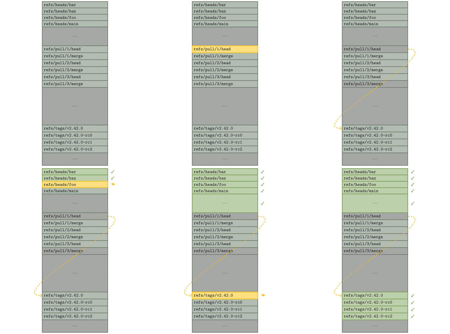
Like the previous example, we still want to discard all of the refs/pull references from the result set. To do so, Git finds the first reference beginning with refs/pull (if one exists), and then performs a modified binary search to find the location of the first reference after all of the ones beginning with refs/pull.
It can then use this information (indicated by the dotted yellow arrow) to avoid looking at the refs/pull hierarchy entirely, providing a measurable speed-up over inspecting and discarding each hidden reference individually.
In Git 2.42, you can try out this new functionality with git for-each-ref‘s new --exclude option. This release also uses this new mechanism to improve the reference advertisement above, as well as analogous components for fetching. In extreme examples, this can provide a 20-fold improvement in the CPU cost of advertising references during a push.
Git 2.42 also comes with a pair of new options in the git pack-refs command, which is responsible for updating the packed-refs file with any new loose references that aren’t stored. In certain scenarios (such as a reference being frequently updated or deleted), it can be useful to exclude those references from ever entering the packed-refs file in the first place.
git pack-refs now understands how to tweak the set of references it packs using its new --include and --exclude flags.
In our last set of release highlights, we talked about a new mechanism for collecting unreachable objects in Git known as cruft packs. Git uses cruft packs to collect and track the age of unreachable objects in your repository, gradually letting them age out before eventually being pruned from your repository.
But Git doesn’t simply delete every unreachable object (unless you tell it to with --prune=now). Instead, it will delete every object except those that meet one of the below criteria:
But what do you do if you want to hold onto an object (or many objects) which are both unreachable and haven’t been modified since the pruning cutoff?
Historically, the only answer to this question was that you should point a reference at those object(s). That works if you have a relatively small set of objects you want to hold on to. But what if you have more precious objects than you could feasibly keep track of with references?
Git 2.42 introduces a new mechanism to preserve unreachable objects, regardless of whether or not they have been modified recently. Using the new gc.recentObjectsHook configuration, you can configure external program(s) that Git will run any time it is about to perform a pruning garbage collection. Each configured program is allowed to print out a line-delimited sequence of object IDs, each of which is immune to pruning, regardless of its age.
Even if you haven’t started using cruft packs yet, this new configuration option works even when using loose objects to hold unreachable objects which have not yet aged out of your repository.
This makes it possible to store a potentially large set of unreachable objects which you want to retain in your repository indefinitely using an external mechanism, like a SQLite database. To try out this new feature for yourself, you can run:
$ git config gc.recentObjectsHook /path/to/your/program
$ git gc --prune=<approxidate>
Over time, many commands have gained support for working with the sparse index. For commands that lacked support for the sparse index, invoking those commands would cause your repository to expand the index to cover the entire repository, which can be a potentially expensive operation.
This release, the diff-tree command joined the group of commands with full support for the sparse index, meaning that you can now use diff-tree without expanding your index.
This work was contributed by Shuqi Liang, one of the Git project’s Google Summer of Code (GSoC) students. You can read more about their project here, and follow along with their progress on their blog.
[source]
If you’ve gotten this far in the blog post and thought that we were done talking about git for-each-ref, think again! This release enhances for-each-ref‘s --format option with a handful of new ways to format a reference.
The first set of new options enables for-each-ref to show a handful of GPG-related information about commits at reference tips. You can ask for the GPG signature directly, or individual components of it, like its grade, the signer, key, fingerprint, and so on. For example,
$ git for-each-ref --format='%(refname) %(signature:key)' \
    --sort=v:refname 'refs/remotes/origin/release-*' | tac
refs/remotes/origin/release-3.1 4AEE18F83AFDEB23
refs/remotes/origin/release-3.0 4AEE18F83AFDEB23
refs/remotes/origin/release-2.13 4AEE18F83AFDEB23
[...]
This work was contributed by Kousik Sanagavarapu, another GSoC student working on Git! You can read more about their project here, and keep up to date with their work on their blog.
Earlier in this post, we talked about git rev-list, a low-level utility for listing the set of objects contained in some query.
In our early examples, we discussed a straightforward case of listing objects unique to one branch. But git rev-list supports much more complex modifiers, like --branches, --tags, --remotes, and more.
In addition to specifying modifiers like these on the command-line, git rev-list has a --stdin mode which allows for reading a line-delimited sequence of commits (optionally prefixed with ^, indicating objects reachable from those commit(s) should be excluded) from the command’s standard input.
Previously, support for --stdin extended only to referring to commits by their object ID, without support for more complex modifiers like the ones listed earlier. In Git 2.42, git rev-list --stdin can now accept the same set of modifiers given on the command line, making it much more useful when scripting.
[source]
Picture this: you’re working away on your repository, typing up a tag message for a tag named foo. Suppose that in the background, you have some repeating task that fetches new commits from your remote repository. If you happen to fetch a tag foo/bar while writing the tag message for foo, Git will complain that you cannot have both tag foo and foo/bar.
OK, so far so good: Git does not support this kind of tag hierarchy1. But what happened to your tag message? In previous versions of Git, you’d be out of luck, since your in-progress message at $GIT_DIR/TAG_EDITMSG is deleted before the error is displayed. In Git 2.42, Git delays deleting the TAG_EDITMSG until after the tag is successfully written, allowing you to recover your work later on.
[source]
In other git tag-related news, this release comes with a fix for a subtle bug that appeared when listing tags. git tag can list existing tags with the -l option (or when invoked with no arguments). You can further refine those results to only show tags which point at a given object with the --points-at option.
But what if you have one or more tags that point at the given object through one or more other tags instead of directly? Previous versions of Git would fail to report those tags. Git 2.42 addresses this by dereferencing tags through multiple layers before determining whether or not it points to a given object.
[source]
Finally, back in Git 2.38, git cat-file --batch picked up a new -z flag, allowing you to specify NUL-delimited input instead of delimiting your input with a standard newline. This flag is useful when issuing queries which themselves contain newlines, like trying to read the contents of some blob by path, if the path contains newlines.
But the new -z option only changed the rules for git cat-file‘s input, leaving the output still delimited by newlines. Ordinarily, this won’t cause any problems. But if git cat-file can’t locate an object, it will print out ” missing”, followed by a newline.
If the given query itself contains a newline, the result is unparseable. To address this, git cat-file has a new mode, -Z (as opposed to its lowercase variant, -z) which changes both the input and output to be NUL-delimited.
[source]
That’s just a sample of changes from the latest release. For more, check out the release notes for 2.42, or any previous version in the Git repository.
$GIT_DIR/refs/tags/foo/bar, it would be impossible to store a tag foo, since it would need to live at $GIT_DIR/refs/tags/foo, which already exists as a directory. ↩
The post Highlights from Git 2.42 appeared first on The GitHub Blog.
Post Syndicated from Eric Washington original https://aws.amazon.com/blogs/security/aws-launched-a-landing-zone-for-the-baseline-informatiebeveiliging-overheid-bio-and-is-issued-a-certificate-for-the-bio-thema-uitwerking-clouddiensten/
We’re pleased to announce that we’ve launched a Landing Zone for the Baseline Informatiebeveiliging Overheid (BIO) framework to support our Dutch customers in their compliance needs with the BIO framework.
We also demonstrated compliance with the BIO Thema-uitwerking Clouddiensten. This alignment with the BIO Thema-uitwerking Clouddiensten requirements demonstrates our continuous commitment to adhere to the heightened expectations for cloud service providers.
Amazon Web Services (AWS) customers across the Dutch public sector can use AWS certified services with confidence, knowing that the AWS services listed in the certificate adhere to the strict requirements imposed on the consumption of cloud-based services.
The BIO framework is an information security framework that the four layers of the Dutch public sector are required to adhere to. This means that it’s mandatory for the Dutch central government, all provinces, municipalities, and regional water authorities to be compliant with the BIO framework.
To support AWS customers in demonstrating their compliance with the BIO framework, AWS developed a Landing Zone for the BIO framework. This Landing Zone for the BIO framework is a pre-configured AWS environment that includes a subset of the technical requirements of the BIO framework. It’s a helpful tool that provides a starting point from which customers can further build their own AWS environment.
For more information regarding the Landing Zone for the BIO framework, see the AWS Reference Guide for Dutch BIO Framework and BIO Theme-elaboration Cloud Services in AWS Artifact. You can also reach out to your AWS account team or contact AWS through the Contact Us page.
In addition to the BIO framework, there’s another information security framework designed specifically for the use of cloud services. It is called BIO Thema-uitwerking Clouddiensten. The BIO Thema-uitwerking Clouddiensten is a guidance document for Dutch cloud service consumers to help them formulate controls and objectives when using cloud services. Consumers can view it as an additional control framework on top of the BIO framework.
AWS was evaluated by the monitoring body, EY CertifyPoint, in February 2023, and it was determined that AWS successfully demonstrated compliance for Amazon Elastic Compute Cloud (Amazon EC2), Amazon Simple Storage Service (Amazon S3), and Amazon Relational Database Service (Amazon RDS) services. The Certificate of Compliance illustrating the compliance status of AWS and the assessment summary report from EY CertifyPoint are available on AWS Artifact. The certificate is available in Dutch and English.
For more information regarding the BIO Thema-uitwerking Clouddiensten, see the AWS Reference Guide for Dutch BIO Framework and BIO Theme-elaboration Cloud Services in AWS Artifact. You can also reach out to your AWS account team or contact AWS through the Contact Us page.
AWS strives to continuously bring services into scope of its compliance programs to help you meet your architectural and regulatory needs.
To learn more about our compliance and security programs, see AWS Compliance Programs. As always, we value your feedback and questions; reach out to the AWS Compliance team through the Contact Us page.
If you have feedback about this post, submit comments in the Comments section below.
Want more AWS Security how-to content, news, and feature announcements? Follow us on Twitter.
Post Syndicated from Stavros Macrakis original https://aws.amazon.com/blogs/big-data/try-semantic-search-with-the-amazon-opensearch-service-vector-engine/
Amazon OpenSearch Service has long supported both lexical and vector search, since the introduction of its kNN plugin in 2020. With recent developments in generative AI, including AWS’s launch of Amazon Bedrock earlier in 2023, you can now use Amazon Bedrock-hosted models in conjunction with the vector database capabilities of OpenSearch Service, allowing you to implement semantic search, retrieval augmented generation (RAG), recommendation engines, and rich media search based on high-quality vector search. The recent launch of the vector engine for Amazon OpenSearch Serverless makes it even easier to deploy such solutions.
OpenSearch Service supports a variety of search and relevance ranking techniques. Lexical search looks for words in the documents that appear in the queries. Semantic search, supported by vector embeddings, embeds documents and queries into a semantic high-dimension vector space where texts with related meanings are nearby in the vector space and therefore semantically similar, so that it returns similar items even if they don’t share any words with the query.
We’ve put together two demos on the public OpenSearch Playground to show you the strengths and weaknesses of the different techniques: one comparing textual vector search to lexical search, the other comparing cross-modal textual and image search to textual vector search. With OpenSearch’s Search Comparison Tool, you can compare the different approaches. For the demo, we’re using the Amazon Titan foundation model hosted on Amazon Bedrock for embeddings, with no fine tuning. The dataset consists of a selection of Amazon clothing, jewelry, and outdoor products.
A search engine is a special kind of database, allowing you to store documents and data and then run queries to retrieve the most relevant ones. End-user search queries usually consist of text entered in a search box. Two important techniques for using that text are lexical search and semantic search. In lexical search, the search engine compares the words in the search query to the words in the documents, matching word for word. Only items that have all or most of the words the user typed match the query. In semantic search, the search engine uses a machine learning (ML) model to encode text from the source documents as a dense vector in a high-dimensional vector space; this is also called embedding the text into the vector space. It similarly codes the query as a vector and then uses a distance metric to find nearby vectors in the multi-dimensional space. The algorithm for finding nearby vectors is called kNN (k Nearest Neighbors). Semantic search does not match individual query terms—it finds documents whose vector embedding is near the query’s embedding in the vector space and therefore semantically similar to the query, so the user can retrieve items that don’t have any of the words that were in the query, even though the items are highly relevant.
The demo of textual vector search shows how vector embeddings can capture the context of your query beyond just the words that compose it.
In the text box at the top, enter the query tennis clothes. On the left (Query 1), there’s an OpenSearch DSL (Domain Specific Language for queries) semantic query using the amazon_products_text_embedding index, and on the right (Query 2), there’s a simple lexical query using the amazon_products_text index. You’ll see that lexical search doesn’t know that clothes can be tops, shorts, dresses, and so on, but semantic search does.

Compare semantic and lexical results
Similarly, in a search for warm-weather hat, the semantic results find lots of hats suitable for warm weather, whereas the lexical search returns results mentioning the words “warm” and “hat,” all of which are warm hats suitable for cold weather, not warm-weather hats. Similarly, if you’re looking for long dresses with long sleeves, you might search for long long-sleeved dress. A lexical search ends up finding some short dresses with long sleeves and even a child’s dress shirt because the word “dress” appears in the description, whereas the semantic search finds much more relevant results: mostly long dresses with long sleeves, with a couple of errors.
The demo of cross-modal textual and image search shows searching for images using textual descriptions. This works by finding images that are related to your textual descriptions using a pre-production multi-modal embedding. We’ll compare searching for visual similarity (on the left) and textual similarity (on the right). In some cases, we get very similar results.
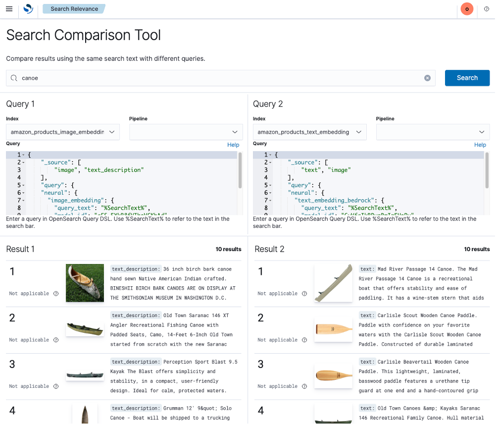
Compare image and textual embeddings
For example, sailboat shoes does a good job with both approaches, but white sailboat shoes does much better using visual similarity. The query canoe finds mostly canoes using visual similarity—which is probably what a user would expect—but a mixture of canoes and canoe accessories such as paddles using textual similarity.
If you are interested in exploring the multi-modal model, please reach out to your AWS specialist.
These demos give you an idea of the capabilities of vector-based semantic vs. word-based lexical search and what can be accomplished by utilizing the vector engine for OpenSearch Serverless to build your search experiences. Of course, production-quality search experiences use many more techniques to improve results. In particular, our experimentation shows that hybrid search, combining lexical and vector approaches, typically results in a 15% improvement in search result quality over lexical or vector search alone on industry-standard test sets, as measured by the NDCG@10 metric (Normalized Discounted Cumulative Gain in the first 10 results). The improvement is because lexical outperforms vector for very specific names of things, and semantic works better for broader queries. For example, in the semantic vs. lexical comparison, the query saranac 146, a brand of canoe, works very well in lexical search, whereas semantic search doesn’t return relevant results. This demonstrates why the combination of semantic and lexical search provides superior results.
OpenSearch Service includes a vector engine that supports semantic search as well as classic lexical search. The examples shown in the demo pages show the strengths and weaknesses of different techniques. You can use the Search Comparison Tool on your own data in OpenSearch 2.9 or higher.
For further information about OpenSearch’s semantic search capabilities, see the following:
 Stavros Macrakis is a Senior Technical Product Manager on the OpenSearch project of Amazon Web Services. He is passionate about giving customers the tools to improve the quality of their search results.