Seven Reasons Your Backup Strategy Might Be Failing You

Post Syndicated from Kari Rivas original https://www.backblaze.com/blog/seven-reasons-your-backup-strategy-might-be-failing-you/
A decorative image showing a cloud with a backup symbol, then three circles with 3, 2, and 1. There are question marks behind the cloud.

Are you confident that your backup strategy has you covered? If not, it’s time to confront the reality that your backup strategy might not be as strong as you think. And even if you’re feeling great about it, it can never hurt to poke holes in your strategy to see where you need to shore up your defenses.

Whether you’re a small business owner wearing many hats (including the responsibility for backing up your company’s data) or a seasoned IT professional, you know that protecting your data is a top priority. The industry standard is the 3-2-1 backup strategy, which states you should have three copies of your data on two different kinds of media with at least one copy off-site or in the cloud. But a lot has changed since that standard was introduced. 

In this post, we’ll identify several ways your 3-2-1 strategy (and your backups in general) could fail. These are common mistakes that even professional IT teams can make. While 3-2-1 is a great place to start, especially if you’re not currently following that approach, it can now be considered table stakes. 

For larger businesses or any business wanting to fail proof its backups, read on to learn how you can plug the gaps in your 3-2-1 strategy and better secure your data from ransomware and other disasters.

Join the Webinar

There’s more to learn about how to shore up your data protection strategy. Join Backblaze on Thursday, August 10 at 10 a.m. PT/noon CT/5 p.m. UTC for a 30-minute webinar on “10 Common Data Protection Mistakes.”

Sign Up ➔ 

Let’s start with a quick review of the 3-2-1 strategy.

The 3-2-1 Backup Strategy

A 3-2-1 strategy means having at least three total copies of your data, two of which are local but on different media, and at least one off-site copy or in the cloud. For instance, a business may keep a local copy of its data on a server at the main office, a second copy of its data on a NAS device in the same location, and a third copy of its data in the public cloud, such as Backblaze B2 Cloud Storage. Hence, there are three copies of its data with two local copies on different media (the server and NAS) and one copy stored off-site in the cloud.
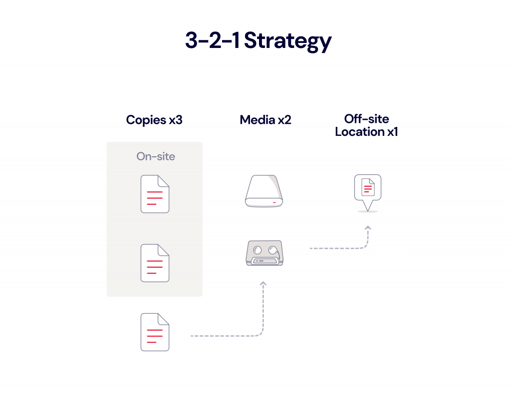
A diagram showing a 3-2-1 backup strategy, in which there are three copies of data, in two different locations, with one location off-site.

The 3-2-1 rule originated in 2005 when Peter Krogh, a photographer, writer, and consultant, introduced it in his book, “The DAM Book: Digital Asset Management for Photographers.” As this rule was developed almost 20 years ago, you can imagine that it may be outdated in some regards. Consider that 2005 was the year YouTube was founded. Let’s face it, a lot has changed since 2005, and today the 3-2-1 strategy is just the starting point. In fact, even if you’re faithfully following the 3-2-1 rule, there may still be some gaps in your data protection strategy.

While backups to external hard drives, tape, and other recordable media (CDs, DVDs, and SD cards) were common two decades ago, those modalities are now considered legacy storage. The public cloud was a relatively new innovation in 2005, so, at first, 3-2-1 did not even consider the possibilities of cloud storage. 

Arguably, the entire concept of “media” in 3-2-1 (as in having two local copies of your data on two different kinds of media) may not make sense in today’s modern IT environment. And, while an on-premises copy of your data typically offers the fastest Recovery Time Objective (RTO), having two local copies of your data will not protect against the multitude of potential natural disasters like fire, floods, tornados, and earthquakes. 

The “2” part of the 3-2-1 equation may make sense for consumers and sole proprietors (e.g., photographers, graphic designers, etc.) who are prone to hardware failure and for whom having a second copy of data on a NAS device or external hard drive is an easy solution, but enterprises have more complex infrastructures. 

Enterprises may be better served by having more than one off-site copy, in case of an on-premises data disaster. This can be easily automated with a cloud replication tool which allows you to store your data in different regions. (Backblaze offers Cloud Replication for this purpose.) Replicating your data across regions provides geographical separation from your production environment and added redundancy. The bottom line is that 3-2-1 is a good starting point for configuring your backup strategy, but it should not be taken as a one-size-fits-all approach.

The 3-2-1-1-0 Strategy

Some companies in the data protection space, like Veeam, have updated 3-2-1 with the 3-2-1-1-0 approach. This particular definition stipulates that you:

  • Maintain at least three copies of business data.
  • Store data on at least two different types of storage media.
  • Keep one copy of the backups in an off-site location.
  • Keep one copy of the media offline or air gapped.
  • Ensure all recoverability solutions have zero errors.
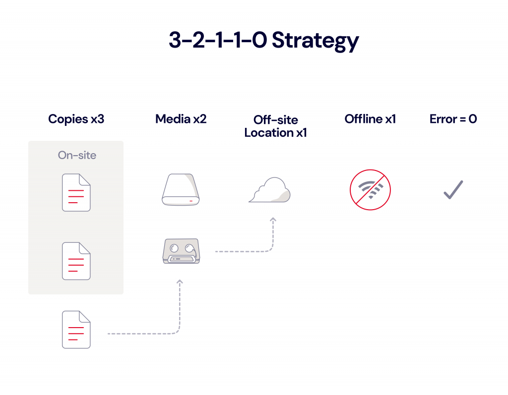
A diagram showing the 3-2-1-1-0 backup strategy.

The 3-2-1-1-0 approach addresses two important weaknesses of 3-2-1. First, 3-2-1 doesn’t address the prevalence of ransomware. Even if you follow 3-2-1 with fidelity, your data could still be vulnerable to a ransomware attack. The 3-2-1-1-0 rule covers this by requiring one copy to be offline or air gapped. With Object Lock, your data can be made immutable, which is considered a virtual air gap, thus fulfilling the 3-2-1-1-0 rule. 

Second, 3-2-1 does not consider disaster recovery (DR) needs. While backups are one part of your disaster recovery plan, your DR plan needs to consider many more factors. The “0” in 3-2-1-1-0 captures an important aspect of DR planning, which is that you must test your backups and ensure you can recover from them without error. Ultimately, you should architect your backup strategy to support your DR plan and the potential need for a recovery, rather than trying to abide by any particular backup rule.

Additional Gaps in Your Backup Strategy

As you can tell by now, there are many shades of gray when it comes to 3-2-1, and these varying interpretations can create areas of weakness in a business’ data protection plan. Review your own plan for the following seven common mistakes and close the gaps in your strategy by implementing the suggested best practices.

1. Using Sync Functionality Instead of Backing Up

You may be following 3-2-1, but if copies of your data are stored on a sync service like Google Drive, Dropbox, or OneDrive, you’re not fully protected. Syncing your data does not allow you to recover from previous versions with the level of granularity that a backup offers.

Best Practice: Instead, ensure you have three copies of your data protected by true backup functionality.

2. Counting Production Data as a Backup

Some interpret the production data to be one of the three copies of data or one of the two different media types.

Best Practice: It’s open to interpretation, but you may want to consider having three copies of data in addition to your production data for the best protection.

3. Using a Storage Appliance That’s Vulnerable to Ransomware

Many on-premises storage systems now support immutability, so it’s a good time to reevaluate your local storage. 

Best Practice: New features in popular backup software like Veeam even enable NAS devices to be protected from ransomware. Learn more about Veeam support for NAS immutability and how to orchestrate end-to-end immutability for impenetrable backups.

4. Not Backing Up Your SaaS Data

It’s a mistake to think your Microsoft 365, Google Workspace, and other software as a service (SaaS) data is protected because it’s already hosted in the cloud. SaaS providers operate under a “shared responsibility model,” meaning they may not back up your data as often as you’d like or provide effective means to recovery. 

Best Practice: Be sure to back up your SaaS data to the cloud to ensure complete coverage of the 3-2-1 rule. 

5. Relying On Off-Site Legacy Storage

It’s always a good idea to have at least one copy of your data on-site for the fastest RTO. But if you’re relying on legacy storage, like tape, to fulfill the off-site requirement of the 3-2-1 strategy, you probably know how expensive and time-consuming it can be. And sometimes that expense and timesuck means your off-site backups are not updated as often as they should be, which leads to mistakes. 

Best Practice: Replace your off-site storage with cloud storage to modernize your architecture and prevent gaps in your backups. Backblaze B2 is one-fifth of the cost of AWS, so it’s easily affordable to migrate off tape and other legacy storage systems.

6. No Plan for Affected Infrastructure

Faithfully following 3-2-1 will get you nowhere if you don’t have the infrastructure to restore your backups. If your infrastructure is destroyed or disrupted, you need a way to ensure business continuity in the face of data disaster.

Best Practice: Be sure your disaster recovery plan outlines how you will access your DR documentation and implement the plan even if your environment is down. Using a tool like Cloud Instant Business Recovery (Cloud IBR), which offers an on-demand, automated solution that allows Veeam users to stand up bare metal servers in the cloud, allows you to immediately begin recovering data while rebuilding infrastructure.

7. Keeping Your Off-Site Copy Down the Street

The 3-2-1 policy states that one copy of your data be kept off-site, and some companies maintain a DR site for that exact purpose. However, if your DR facility is in the same local area as your main office, you have a big gap in your data protection strategy. 

Best Practice: Ideally, you should have an off-site copy of your data stored in a public cloud data center far from your data production site, to protect against regional natural disasters.

Telco Adopts Cloud for Geographic Separation

AcenTek’s existing storage scheme covered the 3-2-1 basics, but their off-site copy was no further away than their own data center. In the case of a large natural disaster, their one off-site copy could be vulnerable to destruction, leaving them without a path to recovery. With Backblaze B2, AcenTek has an additional layer of resilience for its backup data by storing it in a secure, immutable cloud storage platform across the country from their headquarters in Minnesota.

Read the Full Story ➔ 

Modernize Your Backup Strategy

The 3-2-1 strategy is a great starting point for small businesses that need to develop a backup plan, but larger mid-market and enterprise organizations must think about business continuity more holistically. 

Backblaze B2 Cloud Storage makes it easy to modernize your backup strategy by sending data backups and archives straight to the cloud—without the expense and complexity of many public cloud services.

At one-fifth of the price of AWS, Backblaze B2 is an affordable, time-saving alternative to the hyperscalers, LTO, and traditional DR sites. Get started today or contact Sales for more information on Backblaze B2 Reserve, Backblaze’s all-inclusive capacity-based pricing that includes premium support and no egress fees. The intricacies of operations, data management, and potential risks demand a more advanced approach to ensure uninterrupted operations. By leveraging cloud storage, you can create a robust, cost-effective, and flexible backup strategy that you can easily customize to your business needs.

Interested in learning more about backup, business continuity, and disaster recovery best practices? Check out the free Backblaze resources below.

The post Seven Reasons Your Backup Strategy Might Be Failing You appeared first on Backblaze Blog | Cloud Storage & Cloud Backup.
Configure SAML federation for Amazon OpenSearch Serverless with Okta

Post Syndicated from Aish Gunasekar original https://aws.amazon.com/blogs/big-data/configure-saml-federation-for-amazon-opensearch-serverless-with-okta/

Modern applications apply security controls across many systems and their subsystems. Keeping all of these systems in sync would be a major undertaking if you tried to implement it separately. Centralized identity management is the way to maintain a single identity provider (IdP) that can authenticate actors and manage and distribute their rights.

OpenSearch is an open-source search and analytics suite that enables you to ingest, store, analyze, and visualize full text and log data. Amazon OpenSearch Serverless makes it simple to deploy, scale, and operate OpenSearch in the AWS Cloud, freeing you from the undifferentiated heavy lifting of sizing, scaling, and operating an OpenSearch cluster. When you use OpenSearch Serverless, you can integrate with your existing Security Assertion Markup Language 2.0 (SAML)-compliant IdP to provide granular access control for your OpenSearch Serverless collections. Our customers use a variety of IdPs, including AWS IAM Identity Center (successor to AWS SSO), Okta, Keycloak, Active Directory Federation Services (AD FS), and Auth0.

In this post, you will learn how to use Okta as your IdP and integrate it with OpenSearch Serverless to securely manage your users and groups for secure access to your data.

Solution overview

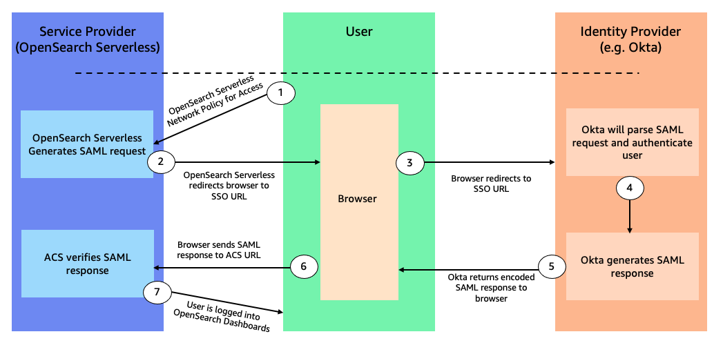
The flow of access requests is depicted in the following figure.

When you navigate to OpenSearch Dashboards, the workflow steps are as follows:

  1. OpenSearch Serverless generates a SAML authentication request.
  2. OpenSearch Serverless redirects your request back to the browser.
  3. The browser redirects to the Okta URL via the Okta application setup.
  4. Okta parses the SAML request, authenticates the user, and generates a SAML response.
  5. Okta returns the encoded SAML response to the browser.
  6. The browser sends the SAML response back to the OpenSearch Serverless Assertion Consumer Services (ACS) URL.
  7. ACS verifies the SAML response and logs in the user with the permissions defined in the data access policy.

Prerequisites

Complete the following prerequisite steps:

  1. Create an OpenSearch Serverless collection. For instructions, refer to Preview: Amazon OpenSearch Serverless – Run Search and Analytics Workloads without Managing Clusters.
  2. Make a note of your AWS account ID to use while configuring your application in Okta.
  3. Create an Okta account, which you will use as an IdP.
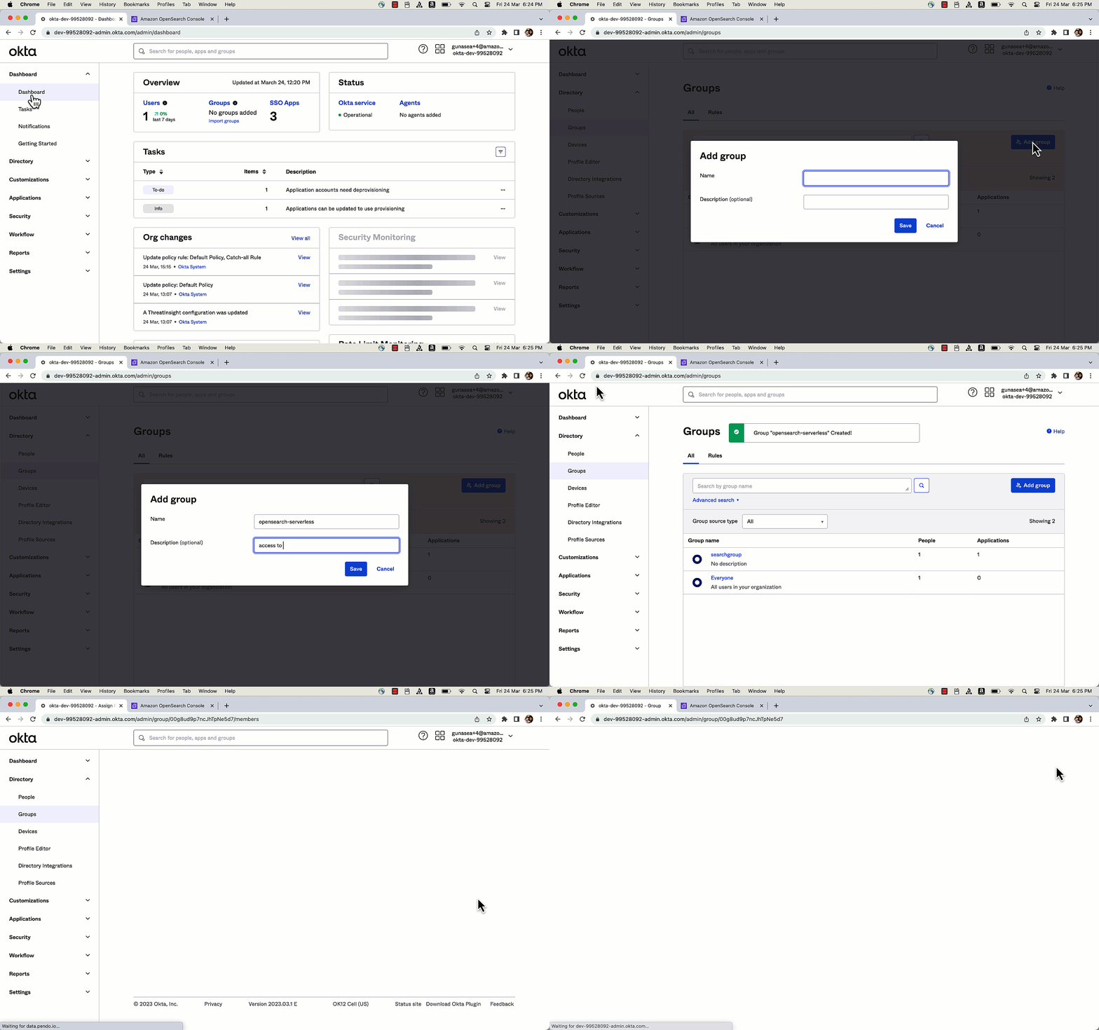
  4. Create users and a group in Okta:
    1. Log in to your Okta account, and in the navigation pane, choose Directory, then choose Groups.
    2. Choose Add Group and name itopensearch-serverless, then choose Save.
    3. Choose Assign People to add users.
    4. You can add users to theopensearch-serverlessgroup by choosing the plus sign next to the user name, or you can choose Add All.
    5. Add your users, then choose Save.
    6. To create new users, choose People in the navigation pane under Directory, then choose Add Person.
    7. Provide your first name, last name, user name (email ID), and primary email address.
    8. For Password, choose Set by admin and First-time password.
    9. To create your user, choose Save.
    10. In the navigation pane, choose Groups, then choose theopensearch-serverless group you created earlier.

The following graphic gives a quick demonstration of setting up a user and group.

Configure an application in Okta

To configure an application in Okta, complete the following steps:

  1. Navigate to the Applications page on the Okta console.
  2. Choose App Integration, select SAML 2.0 web application, then choose Next.
  3. For Name, enter a name for the app (for example, myweblogs), then choose Next.
  4. Under Application ACS URL, enter the URL using the format https://collection.<REGION>.aoss.amazonaws.com/_saml/acs (replace <REGION> with the corresponding Region) to generate the IdP metadata.
  5. Select Use this for Recipient URL and Destination URL to use the same ACS URL as the recipient and destination.
  6. Specify aws:opensearch:<AWS-Account-ID> under Audience URI (SP Entity ID). This specifies who the assertion is intended for within the SAML assertion.
  7. Under Group Attribute Statements, enter a name that is relevant to your application, such as mygroup, and select unspecified as the name format. (Don’t forget this name, you’ll need it later.)
  8. Select equals as the filter and enter opensearch-serverless.
  9. Select I’m a software vendor. I’d like to integrate my app with Okta and choose Finish.
  10. After an app is created, choose the sign-on tab, scroll down to the metadata details, and copy the value for Metadata URL.

The following graphic gives a quick demonstration of setting up an application in Okta via the preceding steps.

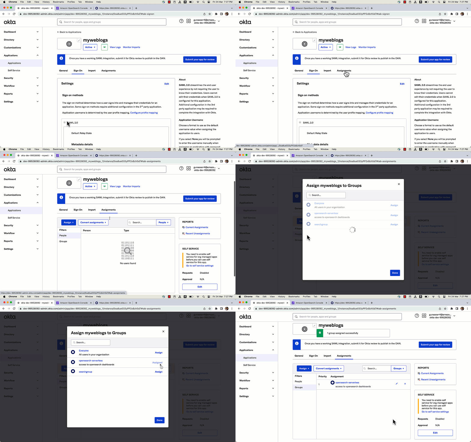
Next, you associate the users and groups to the application that you created in the previous step.

  1. On the Applications page, choose the app you created earlier.
  2. On the Assignments tab, choose Assign.
  3. Select Assign To Groups and choose the group you wish to assign to (opensearch-serverlessin this case).
  4. Choose Done.

The following graphic gives a quick demonstration of assigning groups to the application via the preceding steps.

Set up SAML on OpenSearch Serverless

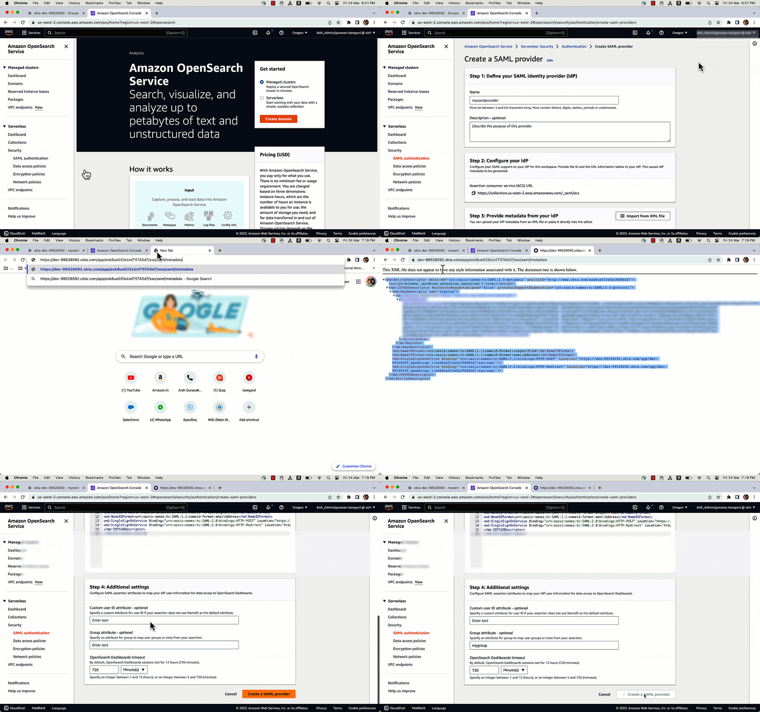
In this section, you create a SAML provider that you’ll use for your OpenSearch Serverless collection. Complete the following steps:

  1. Open the OpenSearch Serverless console on a new tab.
  2. In the navigation pane, under Serverless, choose SAML authentication.
  3. Select Add SAML provider.
  4. Provide a recognizable name (for example, okta) and a description.
  5. Open a new tab and enter the copied metadata URL into your browser.

You should see the metadata for the Okta application.

  1. Take note of this metadata and copy it to your clipboard.
  2. On the OpenSearch Service console tab, enter this metadata in the Provide metadata from your IdP section.
  3. Under Additional settings, enter mygroup or the group attribute provided in the Okta configuration.
  4. Choose Create a SAML provider.

The SAML provider has now been created.

The following graphic gives a quick demonstration of setting up the SAML provider in OpenSearch Serverless via the preceding steps.

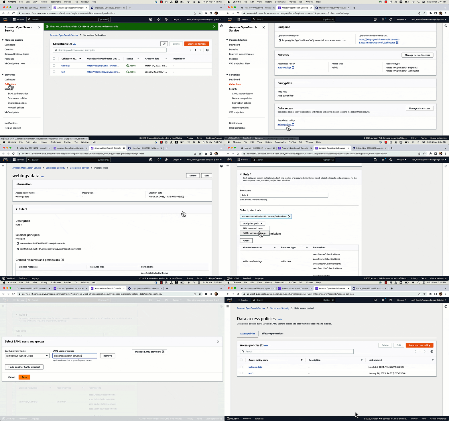
Update the data access policy

You need to configure the right permissions in the data access policies associated with your OpenSearch collection so your Okta group members can access the OpenSearch Dashboards endpoint.

  1. On the OpenSearch Serverless console, open your collection.
  2. Choose the data access policy associated with the collection in the Data Access section.
  3. Choose Edit.
  4. Choose Principals and Add a SAML principal.
  5. Select the SAML provider you created earlier and enter group/opensearch-serverless next to it.
  6. The OpenSearch Dashboards endpoint can be accessed by all group members. You can grant access to collections, indexes, or both.
  7. Choose Save.

Log in to OpenSearch Dashboards

Now that you have set permissions to access the dashboards, choose the Dashboards URL under the general information for the OpenSearch Serverless collection. This should take you to the website
https://collection-endpoint/_dashboards/

You will see a list with all the access options. Choose the SAML provider that you created (okta in this case) and log in using your Okta credentials. You will now be logged into OpenSearch Dashboards with the permissions that are part of the data access policy. You can perform searches or create visualizations from the dashboard.

Clean up

To avoid unwanted charges, delete the OpenSearch Serverless collection, data access policy, and SAML provider created as part of this demonstration.

Summary

In this post, you learned how to set up Okta as an IdP to access OpenSearch Dashboards using SAML. You also learned how to set up users and groups within Okta and configure their access to OpenSearch Dashboards. For more details, refer to SAML authentication for Amazon OpenSearch Serverless.

You can also refer to the Getting started with Amazon OpenSearch Serverless workshop to know more about OpenSearch Serverless.

If you have feedback about this post, submit it in the comments section. If you have questions about this post, start a new thread on the OpenSearch Service forum or contact AWS Support.


About the Authors

Aish Gunasekar is a Specialist Solutions architect with a focus on Amazon OpenSearch Service. Her passion at AWS is to help customers design highly scalable architectures and help them in their cloud adoption journey. Outside of work, she enjoys hiking and baking.

Prashant Agrawal is a Sr. Search Specialist Solutions Architect with Amazon OpenSearch Service. He works closely with customers to help them migrate their workloads to the cloud and helps existing customers fine-tune their clusters to achieve better performance and save on cost. Before joining AWS, he helped various customers use OpenSearch and Elasticsearch for their search and log analytics use cases. When not working, you can find him traveling and exploring new places. In short, he likes doing Eat → Travel → Repeat.

Security updates for Tuesday

Post Syndicated from corbet original https://lwn.net/Articles/940755/

Security updates have been issued by Debian (libhtmlcleaner-java and thunderbird), Red Hat (dbus, kernel, kernel-rt, kpatch-patch, and thunderbird), Scientific Linux (thunderbird), SUSE (chromium, gstreamer-plugins-bad, gstreamer-plugins-base, gstreamer-plugins-good, gstreamer-plugins-ugly, kernel-firmware, libqt5-qtbase, libqt5-qtsvg, librsvg, pcre2, perl-Net-Netmask, qt6-base, and thunderbird), and Ubuntu (firefox).

Project Cybersafe Schools: Bringing security tools for free to small K-12 school districts in the US

Post Syndicated from Zaid Zaid original http://blog.cloudflare.com/project-cybersafe-schools/

Project Cybersafe Schools: Bringing security tools for free to small K-12 school districts in the US

Project Cybersafe Schools: Bringing security tools for free to small K-12 school districts in the US

Like other under-resourced organizations, schools face cyber attacks from malicious actors that can impact their ability to safely perform their basic function: teach children. Schools face email, phishing, and ransomware attacks that slow access and threaten leaks of confidential student data. And these attacks have real effects. In a report issued at the end of 2022, the U.S. Government Accountability Office concluded that schools serving kindergarten through 12th grade (K-12) reported significant educational impact and monetary loss due to cybersecurity incidents, such as ransomware attacks. Recovery time can extend from 2 all the way up to 9 months — that’s almost an entire school year.

Cloudflare’s mission is to help build a better Internet, and we have always believed in helping protect those who might otherwise not have the resources to protect themselves from cyberattack.

It is against this backdrop that we’re very excited to introduce an initiative aimed at small K-12 public school districts: Project Cybersafe Schools. Announced as part of the Back to School Safely: K-12 Cybersecurity Summit at the White House on August 8, 2023, Project Cybersafe Schools will support eligible K-12 public school districts with a package of Zero Trust cybersecurity solutions — for free, and with no time limit. These tools will help eligible school districts minimize their exposure to common cyber threats.

Schools are prime targets for cyberattacks

In Q2 2023 alone, Cloudflare blocked an average of 70 million cyber threats each day targeting the U.S. education sector, and saw a 47% increase in DDoS attacks quarter-over-quarter. In September 2022, the Los Angeles Unified School District suffered a cyber attack, and the perpetrators later posted students’ private information on the dark web. Then, in January 2022, the public school system in Albuquerque, New Mexico was forced to close down for two days following a cyber attack that compromised student data. The list goes on. Between 2016 and 2022, there were 1,619 publicly reported cybersecurity-related incidents aimed at K-12 public schools and districts in the United States.

As an alliance member of the Joint Cyber Defense Collaborative, Cloudflare began conversations with officials from the Cybersecurity & Infrastructure Security Agency (CISA), the Department of Education, and the White House about how we could partner to protect K-12 schools in the United States from cyber threats. We think that we are particularly well-suited to help protect K-12 schools against cyber attacks. For almost a decade, Cloudflare has supported organizations that are particularly vulnerable to cyber threats and lack the resources to protect themselves through projects like Project Galileo, the Athenian Project, the Critical Infrastructure Defense Project, and Project Safekeeping.

Unlike many colleges, universities, and even some larger school districts, smaller school districts often lack the capacity to manage cyber threats. The lack of funding and staff make schools prime targets for hackers. These attacks prevent students from learning, put students’ personal information at risk, and cost school districts time and money in the aftermath of the attacks.

Project Cybersafe Schools: protecting the smallest K-12 public school districts

Project Cybersafe Schools will help support small K-12 public school districts by providing cloud email security to protect against a broad spectrum of threats including Business Email Compromise, multichannel phishing, credential harvesting, and other targeted attacks. Project Cybersafe Schools will also protect against Internet threats with DNS filtering by preventing users from reaching unwanted or harmful online content like ransomware or phishing sites. It can also be deployed to comply with the Children’s Internet Protection Act (CIPA), which Congress passed in 2000, to address concerns about children’s access to obscene or harmful content on the Internet.

We believe that Cloudflare can make a meaningful impact on the cybersecurity needs of our small school districts, which allows the schools to focus on what they do best: teaching students. Hopefully, this project will bring privacy, security, and peace of mind to school managers, staff, teachers, and students, allowing them to focus solely on teaching and learning fearlessly.

What Zero Trust services are available?

Eligible K-12 public school districts in the United States will have access to a package of enterprise-level Zero Trust cybersecurity services for free and with no time limit – there is no catch and no underlying obligations. Eligible organizations will benefit from:

  • Email Protection: Safeguards inboxes with cloud email security by protecting against a broad spectrum of threats including malware-less Business Email Compromise, multichannel phishing, credential harvesting, and other targeted attacks.
  • DNS Filtering: Protects against Internet threats with DNS filtering by preventing users from reaching unwanted or harmful online content like ransomware or phishing sites and can be deployed to comply with the Children’s Internet Protection Act (CIPA).

Who can apply?

To be eligible, Project Cybersafe Schools participants must be:

  • K-12 public school districts located in the United States
  • Up to 2,500 students in the district

If you think your school district may be eligible, we welcome you to contact us to learn more. To apply please visit: https://www.cloudflare.com/lp/cybersafe-schools/

For schools or school districts that do not qualify for Project Cybersafe Schools, Cloudflare has other packages available with educational pricing. If you do not qualify for Project Cybersafe Schools, but are interested in our educational services, please contact us at [email protected].

You Can’t Rush Post-Quantum-Computing Cryptography Standards

Post Syndicated from Bruce Schneier original https://www.schneier.com/blog/archives/2023/08/you-cant-rush-post-quantum-computing-standards.html

I just read an article complaining that NIST is taking too long in finalizing its post-quantum-computing cryptography standards.

This process has been going on since 2016, and since that time there has been a huge increase in quantum technology and an equally large increase in quantum understanding and interest. Yet seven years later, we have only four algorithms, although last week NIST announced that a number of other candidates are under consideration, a process that is expected to take “several years.

The delay in developing quantum-resistant algorithms is especially troubling given the time it will take to get those products to market. It generally takes four to six years with a new standard for a vendor to develop an ASIC to implement the standard, and it then takes time for the vendor to get the product validated, which seems to be taking a troubling amount of time.

Yes, the process will take several years, and you really don’t want to rush it. I wrote this last year:

Ian Cassels, British mathematician and World War II cryptanalyst, once said that “cryptography is a mixture of mathematics and muddle, and without the muddle the mathematics can be used against you.” This mixture is particularly difficult to achieve with public-key algorithms, which rely on the mathematics for their security in a way that symmetric algorithms do not. We got lucky with RSA and related algorithms: their mathematics hinge on the problem of factoring, which turned out to be robustly difficult. Post-quantum algorithms rely on other mathematical disciplines and problems­—code-based cryptography, hash-based cryptography, lattice-based cryptography, multivariate cryptography, and so on­—whose mathematics are both more complicated and less well-understood. We’re seeing these breaks because those core mathematical problems aren’t nearly as well-studied as factoring is.

[…]

As the new cryptanalytic results demonstrate, we’re still learning a lot about how to turn hard mathematical problems into public-key cryptosystems. We have too much math and an inability to add more muddle, and that results in algorithms that are vulnerable to advances in mathematics. More cryptanalytic results are coming, and more algorithms are going to be broken.

As to the long time it takes to get new encryption products to market, work on shortening it:

The moral is the need for cryptographic agility. It’s not enough to implement a single standard; it’s vital that our systems be able to easily swap in new algorithms when required.

Whatever NIST comes up with, expect that it will get broken sooner than we all want. It’s the nature of these trap-door functions we’re using for public-key cryptography.

Updating Fedora the unsupported way

Post Syndicated from Matthew Garrett original https://mjg59.dreamwidth.org/67126.html

I dug out a computer running Fedora 28, which was released 2018-04-01 – over 5 years ago. Backing up the data and re-installing seemed tedious, but the current version of Fedora is 38, and while Fedora supports updates from N to N+2 that was still going to be 5 separate upgrades. That seemed tedious, so I figured I’d just try to do an update from 28 directly to 38. This is, obviously, extremely unsupported, but what could possibly go wrong?

Running sudo dnf system-upgrade download --releasever=38 didn’t successfully resolve dependencies, but sudo dnf system-upgrade download --releasever=38 --allowerasing passed and dnf started downloading 6GB of packages. And then promptly failed, since I didn’t have any of the relevant signing keys. So I downloaded the fedora-gpg-keys package from F38 by hand and tried to install it, and got a signature hdr data: BAD, no. of bytes(88084) out of range error. It turns out that rpm doesn’t handle cases where the signature header is larger than a few K, and RPMs from modern versions of Fedora. The obvious fix would be to install a newer version of rpm, but that wouldn’t be easy without upgrading the rest of the system as well – or, alternatively, downloading a bunch of build depends and building it. Given that I’m already doing all of this in the worst way possible, let’s do something different.

The relevant code in the hdrblobRead function of rpm’s lib/header.c is:

int32_t il_max = HEADER_TAGS_MAX;
int32_t dl_max = HEADER_DATA_MAX;

if (regionTag == RPMTAG_HEADERSIGNATURES) {
il_max = 32;
dl_max = 8192;
}

which indicates that if the header in question is RPMTAG_HEADERSIGNATURES, it sets more restrictive limits on the size (no, I don’t know why). So I installed rpm-libs-debuginfo, ran gdb against librpm.so.8, loaded the symbol file, and then did disassemble hdrblobRead. The relevant chunk ends up being:

0x000000000001bc81 <+81>: cmp $0x3e,%ebx
0x000000000001bc84 <+84>: mov $0xfffffff,%ecx
0x000000000001bc89 <+89>: mov $0x2000,%eax
0x000000000001bc8e <+94>: mov %r12,%rdi
0x000000000001bc91 <+97>: cmovne %ecx,%eax

which is basically “If ebx is not 0x3e, set eax to 0xffffffff – otherwise, set it to 0x2000”. RPMTAG_HEADERSIGNATURES is 62, which is 0x3e, so I just opened librpm.so.8 in hexedit, went to byte 0x1bc81, and replaced 0x3e with 0xfe (an arbitrary invalid value). This has the effect of skipping the if (regionTag == RPMTAG_HEADERSIGNATURES) code and so using the default limits even if the header section in question is the signatures. And with that one byte modification, rpm from F28 would suddenly install the fedora-gpg-keys package from F38. Success!

But short-lived. dnf now believed packages had valid signatures, but sadly there were still issues. A bunch of packages in F38 had files that conflicted with packages in F28. These were largely Python 3 packages that conflicted with Python 2 packages from F28 – jumping this many releases meant that a bunch of explicit replaces and the like no longer existed. The easiest way to solve this was simply to uninstall python 2 before upgrading, and avoiding the entire transition. Another issue was that some data files had moved from libxcrypt-common to libxcrypt, and removing libxcrypt-common would remove libxcrypt and a bunch of important things that depended on it (like, for instance, systemd). So I built a fake empty package that provided libxcrypt-common and removed the actual package. Surely everything would work now?

Ha no. The final obstacle was that several packages depended on rpmlib(CaretInVersions), and building another fake package that provided that didn’t work. I shouted into the void and Bill Nottingham answered – rpmlib dependencies are synthesised by rpm itself, indicating that it has the ability to handle extensions that specific packages are making use of. This made things harder, since the list is hard-coded in the binary. But since I’m already committing crimes against humanity with a hex editor, why not go further? Back to editing librpm.so.8 and finding the list of rpmlib() dependencies it provides. There were a bunch, but I couldn’t really extend the list. What I could do is overwrite existing entries. I tried this a few times but (unsurprisingly) broke other things since packages depended on the feature I’d overwritten. Finally, I rewrote rpmlib(ExplicitPackageProvide) to rpmlib(CaretInVersions) (adding an extra ‘\0’ at the end of it to deal with it being shorter than the original string) and apparently nothing I wanted to install depended on rpmlib(ExplicitPackageProvide) because dnf finished its transaction checks and prompted me to reboot to perform the update. So, I did.

And about an hour later, it rebooted and gave me a whole bunch of errors due to the fact that dbus never got started. A bit of digging revealed that I had no /etc/systemd/system/dbus.service, a symlink that was presumably introduced at some point between F28 and F38 but which didn’t get automatically added in my case because well who knows. That was literally the only thing I needed to fix up after the upgrade, and on the next reboot I was presented with a gdm prompt and had a fully functional F38 machine.

You should not do this. I should not do this. This was a terrible idea. Any situation where you’re binary patching your package manager to get it to let you do something is obviously a bad situation. And with hindsight performing 5 independent upgrades might have been faster. But that would have just involved me typing the same thing 5 times, while this way I learned something. And what I learned is “Terrible ideas sometimes work and so you should definitely act upon them rather than doing the sensible thing”, so like I said, you should not do this in case you learn the same lesson.

comment count unavailable comments

New — Deliver Interactive Real-Time Live Streams with Amazon IVS

Post Syndicated from Donnie Prakoso original https://aws.amazon.com/blogs/aws/new-deliver-interactive-real-time-live-streams-with-amazon-ivs/

Live streaming is becoming an increasingly popular way to connect customers with their favorite influencers and brands through interactive live video experiences. Our customers, DeNA and Rooter, rely on Amazon Interactive Video Service (Amazon IVS), a fully managed live streaming solution, to build engaging live stream and interactive video experiences for their audiences.

In March we introduced Amazon IVS support for multiple hosts in live streams to further provide flexibility in building interactive experiences, by using a resource called stage. A stage is a virtual space where participants can exchange audio and video in real time.

However, latency is still a critical component to engaging audiences and enriching the overall experience. The lower the latency, the better it is to connect with live audiences in a direct and personal way. Previously, Amazon IVS supported real-time live streaming for up to 12 hosts via stages with around 3–5 seconds latency for viewers via channels. This latency gap restricts the ability to build interactive experiences with direct engagement for wider audiences.

Introducing Amazon IVS Real-Time Streaming
Today, I’m excited to share that with Amazon IVS Real-Time Streaming, you now can deliver real-time live streams to 10,000 viewers with up to 12 hosts from a stage, with latency that can be under 300 milliseconds from host to viewer.

This feature unlocks the opportunity for you to build interactive video experiences for social media applications or for latency sensitive use cases like auctions.

Now you will no longer have to compromise to achieve real-time latency for viewers. You can avoid such workarounds as using multiple AWS services or external tools. Instead, you can simply use Amazon IVS as a centralized service to deliver real-time interactive live streams, and you don’t even need to enable anything on your account to start using this feature.

Deliver Real-time Streams with The Amazon IVS Broadcast SDK
To deliver real-time streams, you need to interact with a stage resource and use the Amazon IVS Broadcast SDK available on iOS, Android, and web. With a stage, you can create a virtual space for participants to join as either viewers or hosts with real-time latency that can be under 300 ms.

You can use a stage to build an experience where hosts and viewers can go live together. For example, inviting viewers to become hosts and join other hosts in a Q&A session, delivering a singing competition, or having multiple guests in a talk show.

We published an overview on how to get started with a stage resource on the Add multiple hosts to live streams with Amazon IVS page. Let me do a quick refresher for the overall flow and how to interact with a stage resource.

First, you need to create a stage. You can do this via the console or programmatically using the Amazon IVS API. The following command is an example of how to create a stage using the create-stage API and AWS CLI.

$ aws ivs-realtime create-stage \
    --region us-east-1 \
    --name demo-realtime \
{
    "stage": {
        "arn": "arn:aws:ivs:us-east-1:xyz:stage/mEvTj9PDyBwQ",
        "name": "demo-realtime",
        "tags": {}
    }
}

A key concept for a stage resource that enables participants to join as a host or a viewer is a participation token. A participant token is an authorization token that lets your participants publish or subscribe to a stage. When you’re using the create-stage API, you can also generate a participation token and add additional information by using attributes, including custom user IDs and their display names. The API responds with stage details and participant tokens.

$ aws ivs-realtime create-stage \
    --region us-east-1 \
    --name demo-realtime \
    --participant-token-configurations userId=test-1,capabilities=PUBLISH,SUBSCRIBE,attributes={demo-attribute=test-1}

{
    "participantTokens": [
        {
            "attributes": {
                "demo-attribute": "test-1"
            },
            "capabilities": [
                "PUBLISH",
                "SUBSCRIBE"
            ],
            "participantId": "p7HIfs3v9GIo",
            "token": "TOKEN",
            "userId": "test-1"
        }
    ],
    "stage": {
        "arn": "arn:aws:ivs:us-east-1:xyz:stage/mEvTj9PDyBwQ",
        "name": "demo-realtime",
        "tags": {}
    }
}

In addition to the create-stage API, you can also programmatically generate participant tokens using the API. Currently, there are two capability values for a participant token, PUBLISH and SUBSCRIBE. If you need to invite a participant to host, you need to add a PUBLISH capability while creating the participant token. With the PUBLISH attribute, you can include video and audio of your host into a stream.

Here is an example on how you can generate a participant token.

$ aws ivs-realtime create-participant-token \
    --region us-east-1 \
	--capabilities PUBLISH \
	--stage-arn ARN \
	--user-id test-2

{
    "participantToken": {
        "capabilities": [
            "PUBLISH"
        ],
        "expirationTime": "2023-07-23T23:48:57+00:00",
        "participantId": "86KGafGbrXpK",
        "token": "TOKEN",
        "userId": "test-2"
    }
}

Once you have generated a participant token, you need to distribute it to your respective clients using, for example, a WebSocket message. Then, within your client applications using Amazon IVS Broadcast SDK, you can use this participant token to let the your users join the stage as hosts or viewers. To learn more on how you can interact with a stage resource, you can see and review the sample demo for iOS or Android, and the supporting serverless applications for real-time demo.

At this point, you’re able to deliver real-time live streams using a stage to 10,000 viewers. If you need to extend the stream to a wider audience, you can use your stage as the input for a channel and use the Amazon IVS Low-Latency Streaming capability. With a channel, you can deliver high concurrency video from a single source with low latency that can be under 5 seconds to millions of viewers. You can learn more on how to publish a stage to a channel on the Amazon IVS Broadcast SDK documentation page, which includes information for iOS, Android, and web.

Layered Encoding Feature for Amazon IVS Real-Time Streaming Capability
End users prefer a live stream with good quality. However, the quality of the live stream depends on various factors, such as the health of their network connections and device performance.

The most common scenario is that viewers will receive a single version of video that is above their optimum viewing configuration. For example, if the host can produce high-quality video, the live stream can be enjoyed by viewers with good connections, but viewers with slower connections would experience loading delays or even an inability to watch the videos. However, if the host can only produce low-quality video, viewers with good connections will get less optimal video, while viewers with slower connections will have a better experience.

To address the issue, with this announcement we also released the layered encoding feature for Amazon IVS Real-Time Streaming capability. With layered encoding (also known as simulcast) when you publish to a stage, Amazon IVS will automatically send multiple variations of video and audio. This ensures your viewers can continue to enjoy the stream at the best quality they can receive based on their network conditions.

Customer Voices
During the private preview period, we heard lots of feedback from our customers about Amazon IVS Real-Time Streaming.

Whatnot is a live stream shopping platform and marketplace that allows collectors and enthusiasts to connect with their community to buy and sell products they’re passionate about. “Scaling live video auctions to our global community is one of our major engineering challenges. Ensuring real-time latency is fundamental to maintaining the integrity and excitement of our auction experience. By leveraging Amazon IVS Real-Time Streaming, we can confidently scale our operations worldwide, assuring a seamless and high-quality real-time video experience across our entire user base, whether on web or mobile platforms.”, Ludo Antonov, VP of Engineering.

Available Now
Amazon IVS Real-Time Streaming is available in all AWS Regions where Amazon IVS is available. To use Amazon IVS Real-Time Streaming, you pay an hourly rate for the duration that you have hosts or viewers connected to the stage resource as a participant.

Learn more about benefits, use cases, how to get started, and pricing details for Amazon IVS’s Real-Time Streaming and Low-Latency Streaming capabilities on the Amazon IVS page.

Happy streaming!
— Donnie

Perform time series forecasting using Amazon Redshift ML and Amazon Forecast

Post Syndicated from Tahir Aziz original https://aws.amazon.com/blogs/big-data/perform-time-series-forecasting-using-amazon-redshift-ml-and-amazon-forecast/

Amazon Redshift is a fully managed, petabyte-scale data warehouse service in the cloud. Tens of thousands of customers use Amazon Redshift to process exabytes of data every day to power their analytics workloads.

Many businesses use different software tools to analyze historical data and past patterns to forecast future demand and trends to make more accurate financial, marketing, and operational decisions. Forecasting acts as a planning tool to help enterprises prepare for the uncertainty that can occur in the future.

Amazon Redshift ML makes it easy for data analysts and database developers to create, train, and apply machine learning (ML) models using familiar SQL commands in Amazon Redshift.

With Redshift ML, you can take advantage of Amazon SageMaker, a fully managed ML service, without learning new tools or languages. Simply use SQL statements to create and train SageMaker ML models using your Redshift data and then use these models to make predictions. For more information on how to use Redshift ML, refer to Create, train, and deploy machine learning models in Amazon Redshift using SQL with Amazon Redshift ML.

With Redshift ML, you can now use Amazon Forecast, an ML-based time series forecasting service, without learning any new tools or having to create pipelines to move your data. You can use SQL statements to create and train forecasting models from your time series data in Amazon Redshift and use these models to generate forecasts about revenue, inventory, resource usage, or demand forecasting in your queries and reports.

For example, businesses use forecasting to do the following:

  • Use resources more efficiently
  • Time the launch of new products or services
  • Estimate recurring costs
  • Predict future events like sales volumes and earnings

In this post, we demonstrate how you can create forecasting models using Redshift ML and generate future forecasts using simple SQL commands.

When you use forecasting in Amazon Redshift, Redshift ML uses Forecast to train the forecasting model and to generate forecasts. You pay only the associated Forecast costs. There are no additional costs associated with Amazon Redshift for creating or using Forecast models to generate predictions. View Amazon Forecast pricing for details.

Solution overview

Amazon Forecast is a fully managed time series forecasting service based on machine learning. Forecast uses different ML algorithms to perform complex ML tasks for your datasets. Using historical data, Forecast automatically trains multiple algorithms and produces a forecasting model, also known as a predictor. Amazon Redshift provides a simple SQL command to create forecasting models. It seamlessly integrates with Forecast to create a dataset, predictor, and forecast automatically without you worrying about any of these steps. Redshift ML supports target time series data and related time series data.

As the following diagram demonstrates, Amazon Redshift will call Forecast, and data needed for Forecast model creation and training will be pushed from Amazon Redshift to Forecast through Amazon Simple Storage Service (Amazon S3). When the model is ready, it can be accessed using SQL from within Amazon Redshift using any business intelligence (BI) tool. In our case, we use Amazon Redshift Query Editor v2.0 to create forecast tables and visualize the data.

To show this capability, we demonstrate two use cases:

  • Forecast electricity consumption by customer
  • Predict bike sharing rentals

What is time series data?

Time series data is any dataset that collects information at various time intervals. This data is distinct because it orders data points by time. Time series data is plottable on a line graph and such time series graphs are valuable tools for visualizing the data. Data scientists use them to identify forecasting data characteristics.

Time series forecasting is a data science technique that uses machine learning and other computer technologies to study past observations and predict future values of time series data.

Prerequisites

Complete the following prerequisites before starting:

  1. Make sure you have an Amazon Redshift Serverless endpoint or a Redshift cluster.
  2. Have access to Amazon Redshift Query Editor v2.
  3. On the Amazon S3 console, create an S3 bucket that Redshift ML uses for uploading the training data that Forecast uses to train the model.
  4. Create an AWS Identity and Access Management (IAM role). For more information, refer to Creating an IAM role as the default.

Although it’s easy to get started with AmazonS3FullAccess, AmazonForecastFullAccess, AmazonRedshiftAllCommandsFullAccess, and AmazonSageMakerFullAccess, we recommend using the minimal policy that we have provided (if you already have an existing IAM role, just add it to that role). If you need to use AWS Key Management Service (AWS KMS) or VPC routing, refer to Cluster and configure setup for Amazon Redshift ML administration.

To use Forecast, you need to have the AmazonForecastFullAccess policy. For more restrictive IAM permissions, you can use the following IAM policy:

{
    "Version": "2012-10-17",
    "Statement": [
        {
            "Sid": "VisualEditor0",
            "Effect": "Allow",
            "Action": [
                "forecast:DescribeDataset",
                "forecast:DescribeDatasetGroup",
                "forecast:DescribeAutoPredictor",
                "forecast:CreateDatasetImportJob",
                "forecast:CreateForecast",
                "forecast:DescribeForecast",
                "forecast:DescribeForecastExportJob",
                "forecast:CreateMonitor",
                "forecast:CreateForecastExportJob",
                "forecast:CreateAutoPredictor",
                "forecast:DescribeDatasetImportJob",
                "forecast:CreateDatasetGroup",
                "forecast:CreateDataset",
                "forecast:TagResource",
                "forecast:UpdateDatasetGroup"
            ],
            "Resource": "*"
        } ,
		{
			"Effect": "Allow",
			"Action": [
				"iam:PassRole"
			],
			"Resource":"arn:aws:iam::<aws_account_id>:role/service-role/<Amazon_Redshift_cluster_iam_role_name>"
		}
    ]
}

To allow Amazon Redshift and Forecast to assume the role to interact with other services, add the following trust policy to the IAM role:

{
  "Version": "2012-10-17",
  "Statement": [
    {
      "Effect": "Allow",
      "Principal": {
        "Service": [
          "redshift.amazonaws.com",
           "redshift-serverless.amazonaws.com",
           "forecast.amazonaws.com",
           "sagemaker.amazonaws.com" 
        ]
      },
      "Action": "sts:AssumeRole"
    }
  ]
}[

Use case 1: Forecast electricity consumption

In our first use case, we demonstrate forecasting electricity consumption for individual households. Predicting or forecasting usage could help utility companies better manage their resources and keep them ahead on planning the distribution and supply. Typically, utility companies use software tools to perform the forecasting and perform a lot of steps to create the forecasting data. We show you how to use the data in your Redshift data warehouse to perform predictive analysis or create forecasting models.

For this post, we use a modified version of the individual household electric power consumption dataset. For more information, see ElectricityLoadDiagrams20112014 Data Set (Dua, D. and Karra Taniskidou, E. (2017). UCI Machine Learning Repository [http://archive.ics.uci.edu/ml]. Irvine, CA: University of California, School of Information and Computer Science).

Prepare the data

Refer to the following notebook for the steps needed to create this use case.

Using Query Editor V2, connect to your cluster and open a new notebook.

The data contains measurements of electric power consumption in different households for the year 2014. We aggregated the usage data hourly. Each row represents the total electricity usage for a given household at an hourly granularity.

For our use case, we use a subset of the source data’s attributes:

  • Usage_datetime – Electricity usage time
  • Consumptioninkw – Hourly electricity consumption data in kW
  • Customer_id – Household customer ID

Create the table electricity_consumption and load data using the COPY command:

CREATE TABLE electricity_consumption
(usage_datetime timestamp, 
consumptioninkw float, 
customer_id varchar(24)
);

COPY electricity_consumption
FROM 's3://redshift-blogs/amazon-forecast-blog/electricityusagedata/electricityusagedata.csv'
IAM_ROLE default
REGION 'us-east-1' delimiter ',' IGNOREHEADER 1;

You can verify the dataset by running a SQL query on your table.

As you can notice, the dataset has electricity consumption in the target field (consumptioninkw) at hourly intervals for individual consumers (customer_id).

Create a forecasting model in Redshift ML

We use the Create Model command to create and train a forecast model. For our forecasting dataset, we use electricity consumption data within the FROM clause. See the following code:

CREATE MODEL forecast_electricity_consumption
FROM electricity_consumption 
TARGET consumptioninkw 
IAM_ROLE 'arn:aws:your-IAM-Role'
AUTO ON MODEL_TYPE FORECAST
SETTINGS (S3_BUCKET 'your-S3-bucket-name',
 HORIZON 24,
 FREQUENCY 'H',
 S3_GARBAGE_COLLECT OFF);

Here, the model name is forecast_electricity_consumption. We use the following settings to create the model:

  • Target – The name of the field for prediction.
  • HORIZON – The number of time steps in the future to forecast.
  • FREQUENCY – The forecast frequency, which should match the input frequency in our case (H meaning hourly). Other acceptable frequency values are Y | M | W | D | H | 30min | 15min | 10min | 5min | 1min. For more details, refer to CREATE MODEL with Forecast.

The Create Model command must include one VARCHAR (customer_id) and a timestamp dimension (usage_datetime). All other related time series feature data must be INT or FLOAT data types.

For the Redshift ML forecasting model, make sure that when you issue a CREATE MODEL statement, you specify MODEL_TYPE as FORECAST. When Redshift ML trains a model or predictor on Forecast, it has a fixed forecast, meaning there is not a physical model to compile and run. Therefore, an inference function is not needed for Forecast models. Instead, we show you how you can pull an exported forecast from the training output location in Amazon S3 into a table locally in your Redshift data warehouse.

When using Forecast, the create model command is run in synchronous mode. This means that after the command is run, it will take 10–15 minutes to set up the required Forecast artifacts. The model will then start training in asynchronous mode, meaning that the training is done behind the scenes by Forecast. You can check when the model training is complete by running the show model command:

SHOW MODEL forecast_electricity_consumption;

The following screenshot shows the results.

The model is trained and deployed when status is shown as READY. If you see TRAINING, that means the model is still training and you need to wait for it to complete.

Generate a forecast

After a model has finished training, you can run a simple create table as command to instantiate all the forecast results into a table. This command will get all the forecast results from the S3 bucket where Forecast exported them.

Create the table locally and load the data in the new table:

CREATE TABLE forecast_electricty_predictions AS SELECT FORECAST(forecast_electricity_consumption);

Here, FORECAST is a function that takes your model’s name as input.

Next, check the forecasted data for the next 24 hours:

Select * from forecast_electricity_predictions;

The following screenshot shows the results.

As shown in the preceding screenshot, our forecast is generated for 24 hours because the HORIZON and FREQUENCY parameters at the model creation and training time were defined as 24H, and that can’t change after the model is trained.

Use case 2: Predict bike sharing rentals

Redshift ML supports historical related time series (RTS) datasets. Historical RTS datasets contain data points up to the forecast horizon, and don’t contain any data points within the forecast horizon.

For this use case, we use a modified version of the Bike Sharing Dataset (Fanaee-T,Hadi. (2013). Bike Sharing Dataset. UCI Machine Learning Repository. https://doi.org/10.24432/C5W894).

Our time series dataset contains the event_timestamp and item_id dimensions. It also contains additional attributes, including season, holiday, temperature, and workingday. These features are RTS because they may impact the no_of_bikes_rented target attribute.

For this post, we only include the workingday feature as RTS to help forecast the no_of_bikes_rented target. Based on following chart, we can see a correlation where the number of bikes rented has a direct relationship with working day.

Prepare the data

Refer to the following notebook for the steps needed to create this use case.

Load the dataset into Amazon Redshift using the following SQL. You can use Query Editor v2 or your preferred SQL tool to run these commands.

To create the table, use the following commands:

create table bike_sampledata
(
event_timestamp timestamp,
season float , 
holiday float , 
workingday float , 
weather float , 
temperature float , 
atemperature float, 
humidity float , 
windspeed float , 
casual float , 
registered float , 
no_of_bikes_rented float,
item_id varchar(255)
);

To load data into Amazon Redshift, use the following COPY command:

copy bike_sampledata
from 's3://redshift-blogs/amazon-forecast-blog/bike-data/bike.csv'
IAM_ROLE default
format as csv
region 'us-east-1';

Create a model in Redshift ML using Forecast

For this example, we are not considering any other RTS features and the goal is to forecast the number of bike rentals for the next 24 hours by accounting for the working day only. You can perform analysis and include additional RTS features in the SELECT query as desired.

Run the following SQL command to create your model—note our target is no_of_bikes_rented, which contains the number of total rentals, and we use item_id, event_timestamp, and workingday as inputs from our training set:

CREATE MODEL forecast_bike_consumption 
FROM (
     select
     s.item_id , s.event_timestamp, s.no_of_bikes_rented, s.workingday
     from     
     bike_sampledata s
     )
TARGET no_of_bikes_rented
IAM_ROLE 'arn:aws:your-IAM-Role'
AUTO ON MODEL_TYPE FORECAST
OBJECTIVE 'AverageWeightedQuantileLoss'
SETTINGS (S3_BUCKET 'your-s3-bucket-name',
          HORIZON 24,
          FREQUENCY 'H',
          PERCENTILES '0.25,0.50,0.75,mean',
          S3_GARBAGE_COLLECT ON);

The Create Model command must include one VARCHAR (item_id) and a timestamp dimension (event_timestamp). All other RTS feature data must be INT or FLOAT data types.

The OBJECTIVE parameter specifies a metric to minimize or maximize the objective of a job. For more details, refer to AutoMLJobObjective.

As in the previous use case, the Create Model command will take 10–15 minutes to set up the required Forecast artifacts and then will start the training in asynchronous mode so model training is done behind the scenes by Forecast. You can check if the model is in the Ready state by running the show model command:

SHOW MODEL forecast_bike_consumption;

Generate predictions

After a model has finished training, you can run a Create table command to instantiate all the forecast results into a table. This command gets all the forecast results from the S3 bucket where Forecast exported them.

Create the table locally and load the data in the new table:

CREATE TABLE forecast_bike_consumption_results 
AS SELECT FORECAST(forecast_bike_consumption);

Run following SQL to inspect the generated forecast results:

select * from forecast_bike_consumption_results;

To visualize the data to help us understand it more, select Chart. For the X axis, choose the time attribute and for the Y axis, choose mean.

You can also visualize all the three forecasts together to understand the differences between them:

  1. Choose Trace and choose Time for the X axis and for p50 for the Y axis.
  2. Choose Trace again and choose Time for the X axis and p75 for the Y axis.
  3. Edit the chart title and legend and provide suitable labels.

Clean up

Complete the following steps to clean up your resources:

  1. Delete the Redshift Serverless workgroup or namespace you have for this post (this will also drop all the objects created).
  2. If you used an existing Redshift Serverless workgroup or namespace, use the following code to drop these objects:
    DROP TABLE forecast_electricty_predictions;
    DROP MODEL forecast_electricity_consumption;
    DROP TABLE electricity_consumption;
    DROP TABLE forecast_bike_consumption_results;
    DROP MODEL forecast_bike_consumption;
    DROP TABLE bike_sampledata;

Conclusion

Redshift ML makes it easy for users of all skill levels to use ML technology. With no prior ML knowledge, you can use Redshift ML to gain business insights for your data.

With Forecast, you can use time series data and related data to forecast different business outcomes using familiar Amazon Redshift SQL commands.

We encourage you to start using this amazing new feature and give us your feedback. For more details, refer to CREATE MODEL with Forecast.


About the authors

Tahir Aziz is an Analytics Solution Architect at AWS. He has worked with building data warehouses and big data solutions for over 15 years. He loves to help customers design end-to-end analytics solutions on AWS. Outside of work, he enjoys traveling and cooking.

Ahmed Shehata is a Senior Analytics Specialist Solutions Architect at AWS based on Toronto. He has more than two decades of experience helping customers modernize their data platforms, Ahmed is passionate about helping customers build efficient, performant and scalable Analytic solutions.

Nikos Koulouris is a Software Development Engineer at AWS. He received his PhD from University of California, San Diego and he has been working in the areas of databases and analytics.

Almost a Decade in the Making Our Fanless Intel i3-N305 2.5GbE Firewall Review

Post Syndicated from Patrick Kennedy original https://www.servethehome.com/almost-a-decade-in-the-making-our-fanless-intel-i3-n305-2-5gbe-firewall-review/

We review the biggest advancement in a decade in this fanless Intel Core i3-N305 fanless firewall review and see new storage features as well

The post Almost a Decade in the Making Our Fanless Intel i3-N305 2.5GbE Firewall Review appeared first on ServeTheHome.

Build a serverless retail solution for endless aisle on AWS

Post Syndicated from Sandeep Mehta original https://aws.amazon.com/blogs/architecture/building-serverless-endless-aisle-retail-architectures-on-aws/

In traditional business models, retailers handle order-fulfillment processes from start to finish—including inventory management, owning or leasing warehouses, and managing supply chains. But many retailers aren’t set up to carry additional inventory.

The “endless aisle” business model is an alternative solution for lean retailers that are carrying enough in-store inventory while wanting to avoid revenue loss. Endless aisle is also known as drop-shipping, or fulfilling orders through automated integration with product partners. Such automation results in a customer’s ability to place an order on a tablet or kiosk when they cannot find a specific product of their choice on in-store shelves.

Why is the endless aisle concept important for businesses and customers alike? It means that:

  • Businesses no longer need to stock products more than shelf deep.
  • End customers can easily place an order at the store and get it shipped directly to their home or place of choice.

Let’s explore these concepts further.

Solution overview

When customers are in-store and looking to order items that are not available on shelves, a store associate can scan the SKU code on a tablet. The kiosk experience is similar, where the customer can search for the item themselves by typing in its name.

For example, if a customer visits a clothing store that only stocks the items on shelves and finds the store is out of a product in their size, preferred color, or both, the associate can scan the SKU and check whether the item is available to ship. The application then raises a request with a store’s product partner. The request returns the available products the associate can show to the customer, who can then choose to place an order. When the order is processed, it is directly fulfilled by the partner.

Serverless endless aisle reference architecture

Figure 1 illustrates how to architect a serverless endless aisle architecture for order processing.

Building endless aisle architecture for order processing

Figure 1. Building endless aisle architecture for order processing

Website hosting and security

We’ll host the endless aisle website on Amazon Simple Storage Service (Amazon S3) with Amazon CloudFront for better response time. CloudFront is a content delivery network (CDN) service built for high performance and security. CloudFront can reduce the latency to other AWS services by providing access at the edge and by caching the static content, while dynamic content is provided by Amazon API Gateway integration for our use case. A Web Application Firewall (WAF) is used after CloudFront for protection against internet threats, such as cross-site scripting (XSS) and SQL injection.

Amazon Cognito is used for managing the application user pool, and provides security for who can then access the application.

Solution walkthrough

Let’s review the architecture steps in detail.

Step 1. The store associate logs into the application with their username and password. When the associate or customer scans the bar code/SKU, the following process flow is executed.

Step 2. The front-end application translates the SKU code into a product number and invokes the Get Item API.

Step 3. An invoked getItem AWS Lambda function handles the API call.

This architecture’s design pattern supports multiple partner integration and allows reusability of the code. The design can be integrated with any partner with the ability to integrate using APIs, and the partner-specific transformation is built separately using Lambda functions.

We’ll use Amazon DynamoDB for storing partner information metadata—for example, partner_id, partner_name, partner APIs.

Step 4. The getItem Lambda function fetches partner information from an DynamoDB table. It transforms the request body using a Transformation Lambda function.

Step 5. The getItem Lambda function calls the right partner API. Upon receiving a request, the partner API returns the available product (based on SKU code) with details such as size, color, and any other variable parameter, along with images.

It can also provide links to similar available products the customer may be interested in based on the selected product. This helps retail clients increase their revenue and offer products that aren’t available at a given time on their shelves.

The customer then selects from the available products. Having selected the right product with specific details on parameters such as color, size, quantity, and more, they add them to the cart and begin the check-out process. The customer enters their shipping address and payment information to place an order.

Step 6. The orders are pushed to an Amazon Simple Queue Service (Amazon SQS) queue named create-order-queue. Amazon SQS provides a straightforward and reliable way for customers to decouple and connect micro-services together using queues.

Step 7. Amazon SQS ensures that there is no data loss and orders are processed from the queue by the orders API. The createOrder Lambda function pulls the messages from Amazon SQS and processes them.

Step 8. The orders API body is then transformed into the message format expected by the partner API. This transformation can be done by a Lambda function defined in the configuration in the ‘partners-table’ DynamoDB table.

Step 9. A partner API is called using the endpoint URL, which is obtained from the partners-table. When the order is placed, a confirmation will be returned by the partner API response. With this confirmation, order details are entered in another DynamoDB table called orders-table.

Step 10. With DynamoDB stream, you can track any insert or update to the DynamoDB table.

Step 11. A notifier Lambda function invokes Amazon Simple Email Service (Amazon SES) to notify the store about order activity.

Step 12. The processed orders are integrated with the customer’s ERP application for the reconciliation process. This can be achieved by Amazon Eventbridge rule that invokes a dataSync Lambda function.

Prerequisites

For this walkthrough, you’ll need the following prerequisites:

Build

Locally install CDK library:

npm install -g aws-cdk

Build an Infrastructure package to create deployable assets, which will be used in CloudFormation template.

cd serverless-partner-integration-endless-aisle && sh build.sh

Synthesize CloudFormation template

To see the CloudFormation template generated by the CDK, execute the below steps.

cd serveless-partner-integration-endless-aisle/infrastructure

cdk bootstrap && cdk synth

Check the output files in the “cdk.out” directory. AWS CloudFormation template is created for deployment in your AWS account.

Deploy

Use CDK to deploy/redeploy your stack to an AWS Account.

Set store email address for notifications. If a store wants to get updates about customer orders, they can set STORE_EMAIL value with store email. You will receive a verification email in this account, after which SES can send you order updates.

export STORE_EMAIL=”[email protected]” - Put your email here.

Set up AWS credentials with the information found in this developer guide.

Now run:

cdk deploy

Testing

After the deployment, CDK will output Amazon Cloudfront URL to use for testing.

  • If you have provided STORE_EMAIL address during the set up, then approve the email link received from Amazon SES in your inbox. This will allow order notifications to your inbox.
  • Create a sample user by using the following command, that you can use to login to the website.
    aws cognito-idp admin-create-user --user-pool-id <REACT_APP_USER_POOL_ID> --username <UserName> --user-attributes Name="email",Value="<USER_EMAIL>" Name="email_verified",Value=true
  • The user will receive password in their email.
  • Open CloudFront URL in a web browser. Login to the website with the username and password. It will ask you to reset your password.
  • Explore different features such as Partner Lookup, Product search, Placing an order, and Order Lookup.

Cleaning up

To avoid incurring future charges, delete the resources, delete the cloud formation stack when not needed.

The following command will delete the infrastructure and website stack created in your AWS account:

cdk destroy

Conclusion

In this blog, we demonstrated how to build an in-store digital channel for retail customers. You can now build your endless aisle application using the architecture described in this blog and integrate with your partners, or reach out to accelerate your retail business.

Further reading

Introducing Incus

Post Syndicated from jake original https://lwn.net/Articles/940684/

The Linux Containers project has
announced the addition of
Incus, which is a fork of LXD
5.16 started by Aleksa Sarai. Incus was created in response to Canonical’s removal of LXD from Linux
Containers
.

After some discussion with Aleksa and a fair bit of encouragement from our
community, we have made the decision to take Incus under the umbrella of
Linux Containers and will commit to it the infrastructure which was
previously made available to LXD.

The goal of Incus is to provide a fully community led alternative to
Canonical’s LXD as well as providing an opportunity to correct some
mistakes that were made during LXD’s development which couldn’t be
corrected without breaking backward compatibility.

In addition to Aleksa, the initial set of maintainers for Incus will
include Christian Brauner, Serge Hallyn, Stéphane Graber and Tycho
Andersen, effectively including the entire team that once created LXD.

The Sourceware 25 roadmap

Post Syndicated from corbet original https://lwn.net/Articles/940683/

Sourceware, the development home for
the GNU toolchain and more, is about to celebrate its 25th anniversary and
is looking
forward
to the next 25 years:

That is why in the last couple of years we have started to
diversify our hardware partners, setup new services using
containers and isolated VMs, investigated secure supply chain
issues, added redundant mirrors, created a non-profit home,
collected funds, invested in open communication, open office hours
and introduced community oversight by a Sourceware Project
Leadership Committee with the help from the Software Freedom
Conservancy.

[$] Shadow stacks for 64-bit Arm systems

Post Syndicated from corbet original https://lwn.net/Articles/940403/

Return-oriented
programming (ROP)
has, for some years now, been a valuable tool for
those who would subvert a system’s security. It is thus not surprising
that a lot of effort has gone into thwarting ROP attacks, which depend on
corrupting the call stack with a carefully chosen set of return addresses,
at both the hardware and software levels. One result of this work is
shadow stacks, which can detect corruption of the call stack, allowing the
operating system to react accordingly. The 64-bit Arm implementation of
shadow stacks is called “guarded control stack” (GCS); patches implementing
support for this feature are currently under discussion.

Security updates for Monday

Post Syndicated from jake original https://lwn.net/Articles/940682/

Security updates have been issued by Debian (burp, chromium, ghostscript, openimageio, pdfcrack, python-werkzeug, thunderbird, and webkit2gtk), Fedora (amanda, libopenmpt, llhttp, samba, seamonkey, and xen), Red Hat (thunderbird), Slackware (mozilla and samba), and SUSE (perl-Net-Netmask, python-Django1, trytond, and virtualbox).

Using response streaming with AWS Lambda Web Adapter to optimize performance

Post Syndicated from James Beswick original https://aws.amazon.com/blogs/compute/using-response-streaming-with-aws-lambda-web-adapter-to-optimize-performance/

This post is written by Harold Sun, Senior Serverless SSA, AWS GCR, Xue Jiaqing, Solutions Architect, AWS GCR, and Su Jie, Associate Solution Architect, AWS GCR.

AWS Lambda now supports Lambda response streaming, which introduces a new invocation mode accessible through the Lambda Function URLs. This feature enables Lambda functions to send response content in sequential chunks to the client. It is available for Lambda’s Node.js runtime, custom runtimes, and can be accessed using the InvokeWithResponseStream API in Lambda.

The Lambda Web Adapter, written in Rust, serves as a universal adapter for Lambda Runtime API and HTTP API. It allows developers to package familiar HTTP 1.1/1.0 web applications, such as Express.js, Next.js, Flask, SpringBoot, or Laravel, and deploy them on AWS Lambda. This replaces the need to modify the web application to accommodate Lambda’s input and output formats, reducing the complexity of adapting code to meet Lambda’s requirements.

When using other managed runtimes such as Java, Go, Python, or Ruby, developers can use the Lambda Web Adapter to build applications that support Lambda response streaming more easily.

Implementing response streaming with Lambda Web Adapter

In general, you can regard Lambda Web Adapter as an extension of Lambda, which is integrated into Lambda’s runtime environment using the Lambda Extension API. It operates within an independent process space when the Lambda function is invoked and serves as a custom runtime. When the function is run, the Web Adapter starts alongside the packaged web application.

After initialization, it performs a readiness check on the configured web application’s port every 10ms (the default is 8080, but you can configure other ports using environment variables). Once it receives an HTTP response with an “200 OK” status from the web application, it encapsulates the received Lambda invocation parameters according to the HTTP protocol and sends a request to the running web application.

Once the web application responds to this request, the Web Adapter formats the response content according to the function’s response format and sends it to the client, completing one invocation of the function.

Web adapter architecture

Similarly, the Lambda Web Adapter uses the Custom Runtime API to implement response streaming. When implementing a function using response streaming:

  1. The Web Adapter sends a POST request to the Lambda Runtime’s Response API, including the Lambda-Runtime-Function-Response-Mode HTTP header with the value streaming and the Transfer-Encoding HTTP header with the value chunked:
    POST http://${AWS_LAMBDA_RUNTIME_API}/runtime/invocation/${AwsRequestId}/response
    Lambda-Runtime-Function-Response-Mode: streaming
    Transfer-Encoding: chunked
  2. It encodes the response data according to the HTTP/1.1 Chunked Transfer Encoding protocol specification and sends it as the “Body” to the Lambda Runtime’s Response API.
  3. After assembling the response and completing the data transmission, the Web Adapter closes the underlying network connection.

Under normal circumstances, completing these steps enables Lambda response streaming in a function. However, this is not sufficient for web application scenarios. Web applications must often send custom HTTP response status codes, custom HTTP headers, and some cookie data to the client. The previous steps only achieve streaming of the response body, and cannot add content to the response’s HTTP headers.

To add these, when sending the response content to the Response API, you must:

  1. Add a Content-Type HTTP Header to specify the MIME type (original media type) of the response as application/vnd.awslambda.http-integration-response.
  2. Send the custom response headers, such as HTTP status code, customer headers, and cookies, in JSON format.
  3. Send 8 NULL characters as separators.
  4. Send the response content encoded using the HTTP 1.1 Chunked Transfer Encoding protocol.

Here is an example of the response format:

POST http://${AWS_LAMBDA_RUNTIME_API}/runtime/invocation/${AwsRequestId}/response
Lambda-Runtime-Function-Response-Mode: streaming
Transfer-Encoding: chunked
Content-Type: application/vnd.awslambda.http-integration-response
{
    "statusCode":200,
    "headers":{
        "Content-Type":"text/html",
        "custom-header":"outer space"
    },
    "cookies":[
        "language=xxx",
        "theme=abc"
    ]
}
8 NULL characters
Chunked response body

In Lambda Function URLs, multi-value HTTP headers are not supported. As a result, you cannot implement responses with multi-value HTTP headers in the Lambda Web Adapter.

Using response streaming with Lambda Web Adapter

When packaging Lambda functions using the zip format, you must attach the Lambda Web Adapter as a layer and configure the environment variable AWS_LAMBDA_EXEC_WRAPPER with the value /opt/bootstrap.

After that, you can configure the startup script of the web application as the Lambda function’s handler. By doing this, the function is able to use the Lambda Web Adapter, and the web application can be launched and run within the Lambda runtime environment.

The AWS_LAMBDA_EXEC_WRAPPER environment variable points to the bootstrap script provided by the Web Adapter to ensure the proper execution of the web application.

When using a Docker Image or OCI Image to package the Lambda function, you only need to include the Lambda Web Adapter binary package in the Dockerfile by copying it to the /opt/extensions directory within the image. Additionally, you should specify the port on which the web application listens by setting the PORT environment variable:

COPY --from=public.ecr.aws/awsguru/aws-lambda-adapter:0.7.0 /lambda-adapter /opt/extensions/lambda-adapter

ENV PORT=3000

By default, the Web Adapter is invoked using the buffered mode. To use response streaming as the invocation mode in the function, you must configure an environment variable. Specify the function’s Web Adapter invocation mode as response_stream:

ENV AWS_LWA_INVOKE_MODE=response_stream

Due to the different data formats between the buffered and response stream invocation modes, you must configure the AWS_LWA_INVOKE_MODE to have the same behavior as the InvokeMode specified in the Lambda Function URLs. Otherwise, the client may not process the response content correctly.

Lambda response streaming example

Server-side rendering (SSR) can accelerate the loading time of a React application. With SSR, the the server generates the HTML pages and sends them to the client, which renders the content. The browser executes the hydration process, which “wakes up” the static components from the received HTML and mounts them into the React application. This allows for a faster response to user interactions and improves the overall user experience.

By using Lambda response streaming, your application can achieve a faster TTFB by processing response content in sequential chunks. This helps to reduce the time it takes for the initial data to be sent from the server to the client, enhancing overall performance.

The hydration process can introduce delays as the client-side JavaScript must re-render and rehydrate the page after the initial load. Lambda response streaming minimizes the need for full page hydration, leading to an improved user experience.

Next.js 13’s support for streaming with suspense complements the Lambda response streaming feature, allowing you to use both SSR and selective hydration. This combination can lead to greater improvements in performance and user experience for your Next.js applications.

This GitHub repo demonstrates a Next.js application that supports Lambda response streaming using the Web Adapter and the streaming with suspense feature. Use AWS Serverless Application Model (AWS SAM) to deploy the application to test these optimizations:

git clone [email protected]:aws-samples/lwa-nextjs-response-streaming-example.git
cd lwa-nextjs-response-streaming-example.git

sam build
sam deploy -g --stack-name lambda-web-adapter-nextjs-response-streaming-example

After the sam deploy process is completed, you can access the Lambda Function URLs endpoint provided in the output. Here is the output of the Lambda response streaming Next.js application demo:

Example output

Quotas and pricing

Web Adapter is an enhancement to Lambda and does not incur additional costs. You are only charged for the Lambda function usage based on the resources consumed.

However, response streaming may result in additional network costs. You are billed for any part of the response that exceeds 6MB. For more information, refer to the pricing page.

There is a maximum response size limit of 20MB for Lambda response streaming. This is a soft limit, and you can request to increase this limit by creating a support ticket.

The response speed of Lambda response streaming depends on the size of the response body. The transfer rate for the first 6MB is not limited, but any part of the response beyond 6MB has a maximum throughput of 2MB/s. For more detailed information, refer to Bandwidth limits for response streaming.

Conclusion

Lambda response streaming can improve the TTFB for web pages. With the support of AWS Lambda Web Adapter, developers can more easily package web applications that support Lambda response streaming, enhancing the user experience and performance metrics of their web applications.

For more serverless learning resources, visit Serverless Land.

The collective thoughts of the interwebz