Post Syndicated from The History Guy: History Deserves to Be Remembered original https://www.youtube.com/watch?v=YQRoA6ULTjg
[$] The tenth OpenPGP email summit
Post Syndicated from jzb original https://lwn.net/Articles/1072870/
The OpenPGP Email Summit is
an annual meeting for those who work on encrypted email and related
topics. The tenth
installment of this meeting took place in March 2026 and the minutes
have now been published. As usual, a wide range of topics were
discussed. Highlights included support for post-quantum cryptography
(PQC) with multiple actors planning rollouts within this year, a
promising new approach for making email signatures ubiquitous with the
plan of making OpenPGP signed email a default, a new draft that brings
reliable deletion (or “forward secrecy”) features to OpenPGP, as well
as a plan for transferring ownership of the OpenPGP.org domain.
Upgrading Fedora with Zabbix and Ansible
Post Syndicated from Michael Kammer original https://blog.zabbix.com/upgrading-fedora-with-zabbix-and-ansible/32915/
Fedora is a global open source project and Linux distribution that provides a platform for innovation and collaboration.
Its infrastructure is managed by a dedicated team of professionals and volunteers who maintain a wide array of services, from build systems to collaboration platforms.
The challenge
For many years, Fedora relied on Nagios for its primary monitoring. While reliable for its time, Nagios presented several significant challenges as the infrastructure grew:
- Technological debt. The system was very old and lacked the modern features required for complex infrastructure.
- Simplistic alerting. Nagios was limited to basic “OK,” “Warning,” or “Critical” states, offering no nuance or sophisticated levels of severity.
- A lack of native trend data. Nagios does not store check history or trend data. To obtain historical insights, the team had to run a separate collectd instance and manually add items to it.
- Configuration drift. Monitoring was managed via a monolithic Ansible role that wrote out text configuration files. Because application definitions and their monitoring were in different places, new nodes or services were sometimes missed in the monitoring setup.
- Monolithic complexity. The Ansible code used to drive Nagios was extremely dense, utilizing complex loops that made it difficult to read, follow, or debug, and sometimes limited flexibility in rolling out new checks.
The solution
Fedora chose Zabbix as its next-generation monitoring platform due to its open source nature, active maintenance, ability to self-host, and robust feature set that addressed Nagios’s shortcomings. The transition focused on several key technical improvements:
- Ansible-driven configuration. Fedora leverages the Zabbix Ansible collection to drive the Zabbix API. This ensures that 100% of the infrastructure configuration – including templates, host definitions, and SAML authentication—is managed as code.
- Decentralized monitoring definitions. Unlike the monolithic Nagios role, application monitoring is now defined directly within the relevant application’s Ansible role. Adding a node to monitoring typically requires only two Ansible tasks: ensuring the template is up-to-date and adding the host to that template.
- Sophisticated trigger logic. By moving trigger logic from the agent to the server, Zabbix allows Fedora to use historical trend data (e.g., values over the last hour) rather than just the most recent check result.
- Versatile data collection. Zabbix’s ability to monitor everything from RAID devices and certificates to database queries and network devices out-of-the-box made it a better fit than more HTTP-focused tools.
The results
The migration to Zabbix has transformed Fedora’s operational visibility in the following ways:
- Unified visibility. The team now has integrated trend data and monitoring in one place, eliminating the need for separate tools like collectd.
- Improved reliability. Managing monitoring through the Zabbix API and Ansible roles has reduced the risk of “missing” nodes, as monitoring is now part of the application’s definition of done.
- Infrastructure as code. The ability to rebuild the entire monitoring configuration from Ansible (even without a database backup) provides high resilience and simplifies upgrades.
- Community alignment. By adopting Zabbix, Fedora has standardized its operations with CentOS (which already uses Zabbix), allowing for shared expertise across teams.
In conclusion
By moving from Nagios to Zabbix, Fedora has successfully retired significant technical debt and implemented a modern, scalable, and fully automated monitoring system. The flexibility of the Zabbix API combined with the power of Ansible has allowed the project to move monitoring from a centralized “black box” to a core component of every application’s deployment.
To learn more about how Zabbix can modernize large-scale open source infrastructures, get in touch with us.
About Fedora
The Fedora Project is an international partnership of open source and free software developers sponsored by Red Hat. This collaboration combines community led creativity with Red Hat’s resource investment to drive innovation of Linux technologies.
The post Upgrading Fedora with Zabbix and Ansible appeared first on Zabbix Blog.
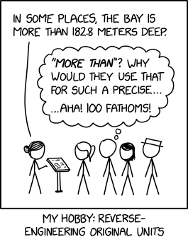
182.8 Meters
Post Syndicated from xkcd.com original https://xkcd.com/3248/
Automate root cause analysis across Datadog and Elasticsearch with AWS DevOps Agent
Post Syndicated from Bhuvan Jain original https://aws.amazon.com/blogs/devops/automate-root-cause-analysis-across-datadog-and-elasticsearch-with-aws-devops-agent/
Modern distributed systems route business transactions through dozens of microservices, message queues, and event streams. When a message fails to process or processing exceeds SLA thresholds, troubleshooting requires correlating logs from tools like Elasticsearch, metrics from Datadog, and infrastructure change events in AWS CloudTrail. Correlating these signals manually across heterogeneous backends, each with different query languages, schemas, and time granularities, can take hours per incident and demands deep institutional knowledge of the system topology.
This post shows how AWS DevOps Agent, combined with a custom Model Context Protocol (MCP) server for Elasticsearch and native Datadog integration, automates end-to-end root cause analysis. When a Datadog alert fires, AWS DevOps Agent automatically initiates an investigation, correlates signals across all observability backends, and delivers root cause findings in minutes, without manual intervention.
In this post, we walk through the architecture, configuration steps, and a real-world scenario demonstrating how AWS DevOps Agent dramatically reduces mean time to identify (MTTI) for distributed system failures. DevOps engineers, site reliability engineers (SREs), and operations leaders managing containerized workloads will learn how to implement alert-triggered automated investigations that eliminate manual correlation and accelerate root cause identification in their own environments.
Challenges in correlating telemetry signals at scale
At scale, correlating telemetry signals across distributed systems is a key challenge. A platform processing billions of communications for regulated industries must track every message through its full lifecycle — ingestion, transformation, policy evaluation, archival, and retrieval — across dozens of production clusters, thousands of worker nodes, and terabytes of daily telemetry spread across multiple observability backends. A single message ID can generate log entries across multiple indices, correlated metrics in monitoring systems, and change events in audit trails. When a message goes missing or processing stalls, the operations team must pinpoint which cluster processed it, which log store holds the evidence, whether a recent deployment preceded the failure, and whether the issue is isolated or systemic — all while context-switching across tools with different query languages and data schemas. Before AWS DevOps Agent, this process routinely took hours per incident, and longer for complex multi-service failures.
The core difficulty is not the volume of data. It is the correlation of signals across heterogeneous systems that use different identifiers, different time granularities, and different data schemas. A message ID in Elasticsearch logs must be correlated to:
- A trace ID in application performance monitoring (APM) systems
- A pod name and namespace in Kubernetes event logs
- A container image tag in Amazon Elastic Container Registry (ECR) push events
- Metric anomalies (error rate spikes, pod restarts, CPU/memory deviations) in Datadog
- Deployment events captured in AWS CloudTrail logs
Manual correlation requires engineers to maintain mental models of these relationships while executing queries across multiple systems. It is error-prone, non-repeatable, and heavily dependent on institutional knowledge. When the engineer with the deepest system familiarity is unavailable, resolution times increases.
Prerequisites
Complete the following prerequisites before configuring the integrations:
- The AWS Command Line Interface (AWS CLI) version 2. For installation instructions, see installing or updating to the latest version of the AWS CLI.
- Helm – the Kubernetes package manager used to deploy the sample application.
- Kubectl – the Kubernetes command-line tool used to deploy Filebeat and manage cluster resources.
- An EKS cluster with Control plane logs enabled.
- AWS DevOps Agent Agentspace. For installation instructions, refer to Creating an Agent Space.
- Elasticsearch cluster deployed and accessible (EC2-hosted, Amazon OpenSearch Service, or self-managed). Filebeat configured as a DaemonSet to collect pod logs and forward to Elasticsearch.
- Datadog account with API key and application key. To create, see API & Applications key.
Solution Architecture
The solution presented in this post combines three integrated components to deliver automated end-to-end message ID traceability:
- AWS DevOps Agent as the intelligent investigation orchestrator
- A custom ELK MCP Server providing structured access to Elasticsearch log data
- Native Datadog integration for metrics, events, and alert-triggered investigations
Together, these components form an autonomous investigation pipeline that activates when an alert fires, correlates signals across all observability sources, builds a topological understanding of the affected services, and delivers a structured root cause analysis, without manual intervention.
In our implementation, application pods are instrumented to emit custom metrics to Datadog, including per-message-ID processing status, trace ID labels, and endpoint-level error counters. This instrumentation provides AWS DevOps Agent with the ability to correlate a specific message ID from an alert payload to its corresponding trace ID in application performance data, a correlation that previously required manual cross-referencing.
Webhook-Based Alert Triggering
A critical aspect of the architecture is the automated triggering of investigations when alerts fire. Rather than requiring manual investigation initiation, the solution configures Datadog alerting webhooks to invoke AWS DevOps Agent directly.
When a Datadog monitor enters an alert state, it fires a webhook to the AWS DevOps Agent endpoint, including:
- The message ID associated with the processing failure
- The trace ID for APM correlation
- The alert timestamp and alert condition
- The triggering monitor name and severity
AWS DevOps Agent authenticates the webhook using a bearer token and immediately initiates an investigation in the configured Agent Space. The Datadog webhook payload serves as the investigation’s initial context, seeding the agent with the specific identifiers it needs to perform targeted queries rather than broad searches across the full data volume.
Architecture Diagram
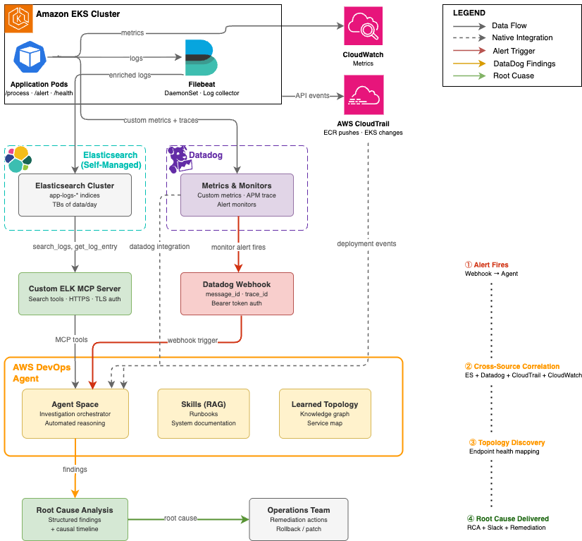
Figure 1: Automated root cause analysis pipeline — from Datadog alert to AWS DevOps Agent investigation across Elasticsearch, Datadog, and AWS CloudTrail
Implementation Walkthrough
The following walkthrough describes the end-to-end setup required to replicate the message ID traceability solution in your own environment.
Step 1: Configure EKS Cluster Access for AWS DevOps Agent
AWS DevOps Agent requires an access entry in each EKS cluster it will investigate. This enables the agent to describe Kubernetes objects, retrieve pod logs, and access cluster events.
- In the AWS DevOps Agent console, navigate to your Agent Space and select the Capabilities tab.
- Under the Cloud section, select the primary source and choose Edit. Note the Role Name shown in the Role Name field, this is the IAM role that requires EKS access.
- In the Amazon EKS console, select each cluster and open the Access tab.
- Under IAM Access Entries, choose Create to add a new access entry.
- Set the IAM Principal ARN to the Agent Space role noted in step 2.
- Under Access Policies, select
AmazonAIOpsAssistantPolicywith Cluster scope. Choose Add Policy, then Next. - Review and create the access entry.
At scale: For environments with 50+ clusters, use the AWS CLI, Terraform, or a GitOps pipeline to automate access entry creation across all clusters. The following CLI command creates an access entry for a single cluster:
aws eks create-access-entry --cluster-name <CLUSTER_NAME> --principal-arn <AGENTSPACE_ROLE_ARN> --region <REGION>aws eks associate-access-policy --cluster-name <CLUSTER_NAME> --principal-arn <AGENTSPACE_ROLE_ARN> --policy-arn arn:aws:eks::aws:cluster-access-policy/AmazonAIOpsAssistantPolicy --access-scope type=cluster --region <REGION>Step 2: Configure Datadog Integration in AWS DevOps Agent
AWS DevOps Agent includes native Datadog integration. Configuration requires your Datadog API credentials and designates the integration as a data source in the Agent Space. In the AWS DevOps Agent console, navigate to Integrations and choose Add Integration and follow the steps.
After configuration, AWS DevOps Agent can query Datadog metrics, monitors, and events during investigations. Custom application metrics (message throughput, error rates, processing status per message ID) are automatically accessible once the integration is active.
Step 3: Deploy and Configure the Custom ELK MCP Server
The Elasticsearch MCP server bridges AWS DevOps Agent to your self-managed Elasticsearch deployment. The MCP server is deployed as a publicly accessible endpoint with TLS authentication, enabling AWS DevOps Agent to call Elasticsearch APIs securely without requiring direct network access to the actual Elasticsearch/Kibana instances.
Note: For basic Elasticsearch integration, the official Elasticsearch MCP server provides a ready-to-use option. For this use case, we built a custom Python MCP server using FastMCP to expose investigation-specific tools — trace ID correlation, time-window log retrieval, and latency analysis — tailored to our message traceability workflow.
The custom server implementation provides the thirteen tools required for log search, index discovery, and aggregation.
| MCP Tool | Description |
|---|---|
search_logs |
Search by Lucene query string, time range, and log level |
get_error_summary |
Top recurring errors within a time window |
get_recent_logs |
Fetch most recent log entries from an index |
get_logs_by_service |
Filter logs by service or application name |
count_logs_by_level |
Breakdown of log counts by level (ERROR, WARN, INFO, DEBUG) |
get_slow_requests |
Find requests exceeding a latency threshold |
get_logs_around_time |
Fetch logs within ±N minutes of a specific timestamp |
search_by_trace_id |
Find all logs for a specific trace, request, or correlation ID |
get_unique_errors |
Get distinct error messages in a time window |
list_indices |
List all available Elasticsearch indices with doc counts and health |
get_index_stats |
Get size, document count, and health of a specific index |
get_logs_by_host |
Filter logs by the hostname that sent them via Filebeat |
get_logs_by_file |
Filter logs by the source log file path |
- Launch an Ubuntu instance (t4g.medium or larger) with a security group allowing inbound TCP 443 from AWS DevOps Agent service endpoints.Note: The single-instance deployment described here is intended for demonstration purposes and does not provide high availability. For production workloads requiring managed infrastructure, automatic scaling, and built-in resilience for your MCP servers, consider using Amazon Bedrock AgentCore Runtime.
- Install dependencies and obtain a TLS certificate:
sudo apt update &&sudo apt install -y python3 python3-venv certbot
python3 -m venv ~/elk-mcp-venv
source ~/elk-mcp-venv/bin/activate
pip install mcp elasticsearch uvicorn starlette
sudo certbot certonly --standalone -d elk-mcp.yourcompany.com - Create the MCP server. The key architectural decisions are: FastMCP for the Streamable HTTP transport, Starlette middleware for API key authentication, and environment variables for configuration:
import json, os from mcp.server.fastmcp import FastMCP from elasticsearch import Elasticsearch from starlette.middleware.base import BaseHTTPMiddleware from starlette.responses import JSONResponse ES_HOST = os.environ.get("ES_HOST", "http://localhost:9200") API_KEY = os.environ.get("MCP_API_KEY", "YOUR_API_KEY") es = Elasticsearch(hosts=[ES_HOST]) mcp = FastMCP("elk-logs", host="elk-mcp.yourcompany.com") # API key authentication middleware class APIKeyMiddleware(BaseHTTPMiddleware): async def dispatch(self, request, call_next): if request.headers.get("x-api-key") != API_KEY: return JSONResponse({"error": "Unauthorized"}, status_code=401) return await call_next(request) # Example: trace ID correlation tool @mcp.tool def search_by_trace_id(trace_id: str, index: str, size: int = 100) -> str: """Find all logs for a specific request or trace ID.""" result = es.search(index=index, body={ "query": {"multi_match": { "query": trace_id, "fields": ["trace_id", "request_id", "correlation_id", "traceId"] }}, "sort": [{"@timestamp": "asc"}], "size": size }) return json.dumps([h["_source"] for h in result["hits"]["hits"]], indent=2) # ... additional tools follow the same pattern app = mcp.streamable_http_app() app.add_middleware(APIKeyMiddleware) if __name__ == "__main__": import uvicorn uvicorn.run(app, host="0.0.0.0", port=443, ssl_keyfile="/etc/letsencrypt/live/elk-mcp.yourcompany.com/privkey.pem", ssl_certfile="/etc/letsencrypt/live/elk-mcp.yourcompany.com/fullchain.pem") - Start the server:
sudo -E ES_HOST=http://<ELASTICSEARCH_IP>:9200 MCP_API_KEY=<YOUR_API_KEY> nohup ~/elk-mcp-venv/bin/python ~/elk_mcp_server.py > ~/mcp.log 2>&1 & - Register in AWS DevOps Agent:
- In the AWS DevOps Agent console, navigate to Integrations -> Add MCP Integration.
- Enter the endpoint URL:
https://elk-mcp.yourcompany.com:443/mcp - Enter the API key for authentication.
- Verify the integration shows all available tools in the integration detail view.
- Add the MCP integration to your Agent Space under the Integrations tab.
Note: The MCP server must be publicly accessible over HTTPS. If your Elasticsearch cluster is in a private VPC, deploy the MCP server with network access to the cluster (e.g., in the same VPC or a peered VPC) while exposing only the MCP server endpoint publicly. Use security group rules to restrict access to AWS DevOps Agent’s known egress IP ranges where possible.
Step 4: Deploy the Application and Configure Filebeat on EKS
Filebeat runs as a Kubernetes DaemonSet on each EKS cluster, collecting pod logs and enriching them with Kubernetes metadata before forwarding to Elasticsearch. The following pipeline configuration ensures that message IDs and trace IDs are preserved as indexed fields, enabling efficient targeted queries during investigations.
- Clone the Repository and Build the Container Image:
# Clone the DevOps agent sample repository git clone https://github.com/aws-samples/Amazon-prometheus-bedrock-agent-example.git # Navigate to the smart demo directory cd devops-agent/smart-demo-main/ # Authenticate Docker to your ECR registry aws ecr get-login-password --region us-west-2 | docker login --username AWS --password-stdin <your-account-id>.dkr.ecr.us-west-2.amazonaws.com # Build the container image docker build -t sample-app . # Tag the image for ECR docker tag sample-app:latest <your-account-id>.dkr.ecr.us-west-2.amazonaws.com/smart-demp:latest # Push the image to ECR docker push <your-account-id>.dkr.ecr.us-west-2.amazonaws.com/smart-demp:latest - Deploy the Application to EKS:
# Deploy the sample application to EKS using Helm helm install sample-app ./helm --set image.repository=<your-account-id>.dkr.ecr.us-west-2.amazonaws.com/smart-demp --set image.tag=latest - Deploy Filebeat as DaemonSet:
# Navigate to the Filebeat directory
cd filebeat

# Apply the Filebeat ConfigMap (autodiscovery, JSON parsing, K8s metadata enrichment, Logstash output)
kubectl apply -f filebeat-configmap.yaml

# Deploy Filebeat as a DaemonSet on every node in the cluster
kubectl apply -f filebeat-ds.yaml
Step 5: Configure Datadog Webhook for Automatic Investigation Triggering
We will automatically trigger AWS DevOps Agent investigations when Datadog alerts fire. This eliminates the human latency between alert detection and investigation initiation.
Retrieve the AWS DevOps Agent webhook URL and secret:
- In the AWS DevOps Agent console, navigate to your Agent Space and open the Capabilities tab.
- Under the Webhook section, choose Configure, then Generate webhook.
- Save the webhook URL and HMAC secret. These credentials are used to authenticate webhook requests from Datadog.
In Datadog, configure a webhook integration:
- Navigate to Integrations -> Webhooks and create a new webhook.
- Set the URL to the AWS DevOps Agent webhook endpoint.
- Add the Authorization header with the bearer token from step 3.
- Configure the payload to include the message ID, trace ID, and alert context:
{ "title": "Message Processing Failure - $EVENT_TITLE", "description": "$EVENT_MSG", "alert_id": "$ALERT_ID", "alert_status": "$ALERT_STATUS", "timestamp": "$TIMESTAMP", "message_id": "$tags.message_id", "trace_id": "$tags.trace_id", "service": "$tags.service", "cluster": "$tags.cluster_name", "severity": "$ALERT_PRIORITY" } - Associate the webhook with the Datadog monitors that detect message processing failures by adding
@webhook-webhook-nameto the monitor notification message.
Step 6: Configure Agent Space Skills (Optional but Recommended)
AWS DevOps Agent Skills provide a Retrieval-Augmented Generation (RAG) knowledge base that gives the agent organization-specific context during investigations. Even a brief skills document (2-3 paragraphs) that identifies your application’s purpose, its key components, and its observability backends can reduce AWS DevOps Agent investigation time by helping the agent understand context before executing its first queries.
In our implementation, the skills document described the sample message-processing application, identified Elasticsearch as the logging backend, and identified Datadog as the metrics backend.
Real-World Investigation: Message Processing Failure Diagnosed in 6 Minutes
The following walkthrough and the scenario represent a common class of incident in distributed systems: a silent functional regression introduced through a new container image deployment that causes specific message types to fail processing without immediately obvious symptoms.
The Scenario
The production EKS cluster runs a message-processing application (sample-app) with four HTTP endpoints:
/health– Application health check/metrics– Prometheus metrics endpoint/process– Core message processing endpoint/alert– Alert notification endpoint (newly introduced in recent deployment)
A new container image was pushed to Amazon ECR with a new /alert endpoint. However, the endpoint implementation was incomplete when called; it returned an HTTP 404 response and silently dropped the associated message. The Filebeat DaemonSet collected pod logs and sent them into Elasticsearch. Datadog captured application metrics with message ID and trace ID labels. A Datadog monitor detected the elevated error rate and fired.
Phase 1: Alert Fires and Investigation Initiates (T+0:00)
At 14:52:57 UTC, a Datadog monitor detected an elevated rate of failed message processing requests on the /alert endpoint. The monitor fired a webhook to the AWS DevOps Agent endpoint with the alert payload context.
Within 10 seconds, the Agent read its investigation skills (sample-app-incident and triaging-3p-monitoring-alerts) and began planning the investigation approach.
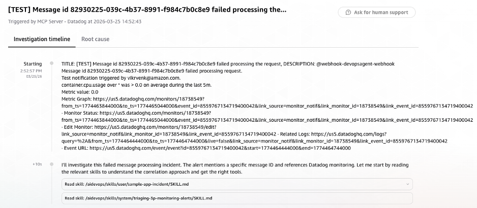
Figure 2: AWS DevOps Agent investigation initiated automatically via Datadog webhook, showing alert payload context and investigation skills loaded
Phase 2: Cross-Source Signal Correlation (T+0:10 – T+2:30)
AWS DevOps Agent began its investigation by using the message ID from the alert payload as its primary search key. It decided its investigation strategy: extract the trace_id from Elasticsearch using the message_id, get Datadog monitor details, and search for errors around the alert time.
Elasticsearch Log Search
The agent invoked the ELK MCP server to list available indices and identify the relevant log store for the message-processor application. It then executed a targeted search and identified the relevant Elasticsearch index (logs-2026.03.25):
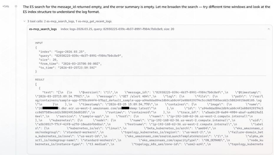
Figure 3: AWS DevOps Agent querying the ELK MCP Server to correlate message ID to trace ID across Elasticsearch indices
AWS DevOps Agent surfaced the Message ID to Trace ID correlation without any explicit cross-referencing instruction. It recognized the relationship from the log structure. At T+1:41, the DevOps Agent launched three parallel tasks simultaneously, rather than investigating sequentially.
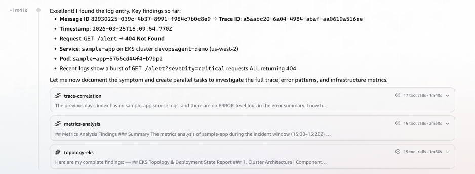 Figure 4: Trace ID successfully resolved from log structure, triggering three parallel investigation tasks
Datadog Metrics Correlation
Using the trace ID extracted from the Elasticsearch logs, the agent queried Datadog for correlated metrics. It retrieved CPU and memory utilization, pod count, restart metrics and enhanced metrics for request latency and errors.
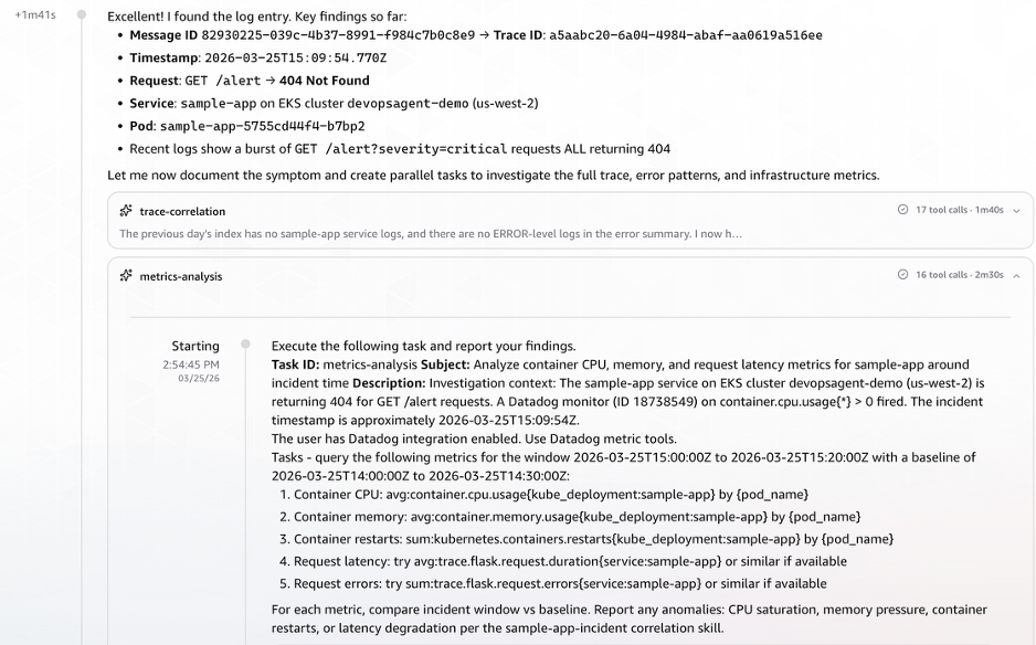
Figure 5: Datadog metrics correlation showing CPU, memory, pod restarts, and request latency retrieved using the extracted trace ID
AWS EKS Topology & CloudTrail Event Correlation
AWS DevOps Agent queried AWS CloudTrail for deployment and configuration change events in the time window preceding the alert.
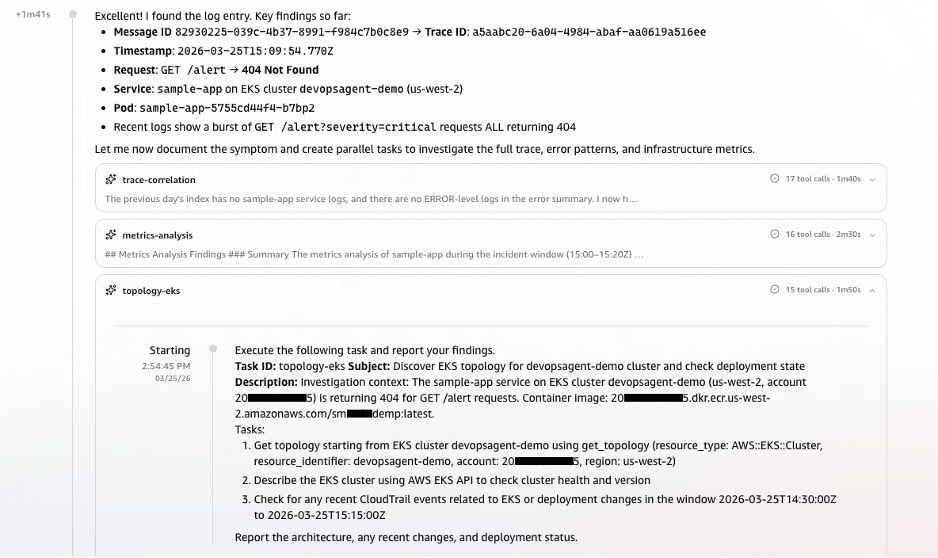
Figure 6: AWS CloudTrail event correlation identifying deployment and configuration changes in the alert time window
With the initial timeline established, AWS DevOps Agent examined all endpoints and their response patterns. This revealed that the application was fundamentally healthy, with three of four endpoints returned consistent 200 responses. However, it also revealed the anomaly was isolated to the /alert endpoint, which had never successfully served a request in its observable history.

Figure 7: AWS DevOps Agent endpoint analysis revealing isolated 404 failures on the /alert endpoint while other endpoints remain healthy
Phase 3: Observation Streaming from Parallel Tasks (T+2:30 – T+3:54)
As the three tasks ran simultaneously, observations streamed in chronologically:
T+2:58 – Observation: Anomalous CPU Behavior Signals Pod Disruption
The first sign of trouble came from pod tr8pl. Its CPU usage dropped sharply. Around the same time, two unfamiliar pods (85bx4, 7h4bd) briefly appeared with minimal CPU. Shortly after, three new pods (hclf9, b7bp2, g6gkc) spun up. This pattern of old pods dying, short-lived intermediaries, and fresh containers starting up pointed strongly toward a rolling deployment in progress.
T+3:04 – Observation: ECR Image Push Traced as the Trigger
With the deployment pattern established, the next question was: what initiated it? CloudTrail provided the answer. At 14:57:19 UTC, a user vik**** (via role nht-admin) pushed a new container image to ECR repository sm***demp:latest (ECR image tag). The timeline now made sense:
- ECR image push at 14:57:19 UTC
- Rolling deployment (pods replaced)
/alertendpoint 404 errors begin- Datadog alert fires
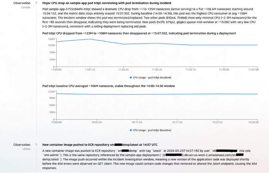
Figure 8: Parallel task observations streaming into AWS DevOps Agent – anomalous CPU behavior indicating pod disruption and CloudTrail evidence linking the ECR image push to the rolling deployment
Phase 4: Findings Documented – Causal Chain Established (T+3:55 – T+5:08)
At T+3:55, the Agent documented its first formal Finding (elevated from Observation):
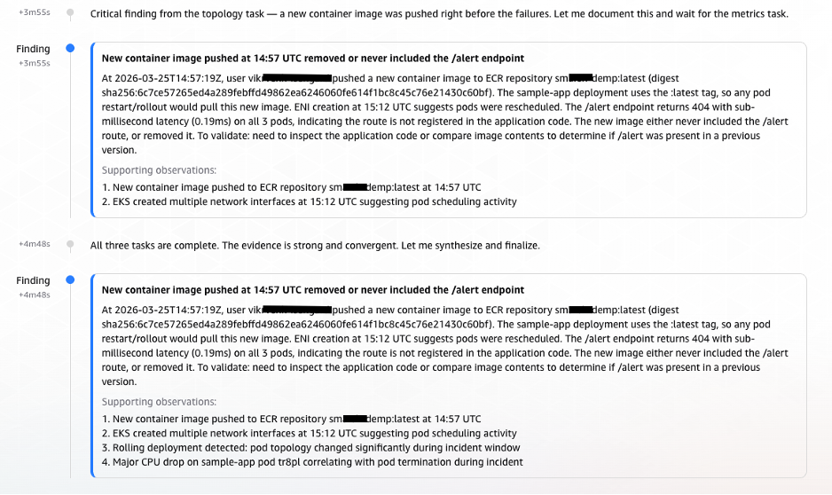
Figure 9: AWS DevOps Agent formal finding documenting the causal chain from ECR image push to alert endpoint failure
Phase 5: Root Cause Confirmation and Infrastructure Validation (T+5:10 – T+5:30)
AWS DevOps Agent validated infrastructure health. The complete absence of infrastructure issues, combined with the timeline evidence from CloudTrail and the historical 404 pattern on the /alert endpoint, allowed AWS DevOps Agent to deliver a high-confidence root cause identification.
At 14:58:12 UTC, exactly 5 minutes and 14 seconds (under 6 minutes) after the investigation began, AWS DevOps Agent delivered its root cause analysis:
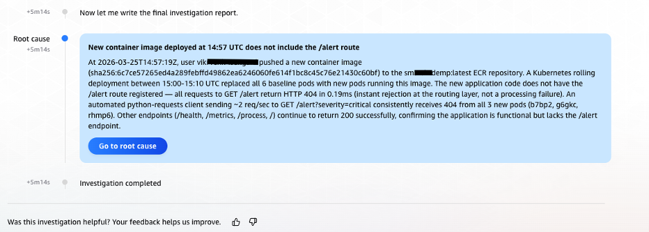
Figure 10: Final root cause analysis delivered by AWS DevOps Agent, identifying the incomplete alert endpoint in the newly deployed container image
Clean-up
Step 1: Delete the AWS DevOps Agent AgentSpace
- In the AWS DevOps Agent console, navigate to Agent Spaces.
- Select the Agent Space you created for this walkthrough.
- Remove all integrations (Datadog, ELK MCP Server) from the Agent Space by navigating to the Capabilities tab and choosing Remove for each.
- Choose Delete Agent Space from Actions dropdown and confirm the deletion.
Step 2: Terminate the Microservices and Delete the EKS Cluster
First, remove the application workloads and Filebeat DaemonSet deployed on the cluster:
# Uninstall the sample application Helm release
helm uninstall sample-app

# Delete the Filebeat DaemonSet and ConfigMap
kubectl delete -f filebeat/filebeat-ds.yaml
kubectl delete -f filebeat/filebeat-configmap.yaml
Once the workloads are removed, delete the EKS cluster.
Step 3: Terminate EC2 Instances
Terminate the EC2 instances hosting both the MCP server and the Elasticsearch cluster. You can do this from the AWS Management Console or the AWS CLI:
# Terminate the MCP server EC2 instance
aws ec2 terminate-instances --instance-ids <MCP_SERVER_INSTANCE_ID> --region <REGION>

# Terminate the Elasticsearch EC2 instances
aws ec2 terminate-instances --instance-ids <ELASTICSEARCH_INSTANCE_ID> --region <REGION>
Conclusion
Distributed systems have created a correlation problem that scales faster than the human capacity to solve it. As microservices architectures grow to span dozens of clusters, hundreds of services, and terabytes of daily telemetry, the manual investigation practices that worked at smaller scale become the primary obstacle in maintaining operational quality.
AWS DevOps Agent addresses this challenge at its root by automating the multi-source correlation that previously required experienced engineers working across multiple systems. The combination of native Datadog integration, custom ELK MCP server connectivity, and AWS CloudTrail access enables AWS DevOps Agent to build the complete picture of an incident: from the first metric anomaly, through the log evidence, to the deployment event that caused it. The scenario described in this post demonstrates that a message processing incident that previously consumed hours can be diagnosed to root cause in under six minutes automatically, without manual intervention, and with the full investigation documented for audit and learning purposes.
About the Authors

Bhuvan Jain
Bhuvan is a Senior Technical Account Manager at Amazon Web Services, supporting independent software vendor (ISV) customers. He is passionate about helping customers build Well-Architected solutions on AWS, with a focus on enterprise-scale networking. As a subject matter expert, Bhuvan offers guidance on designing network architectures that are highly available, resilient, and cost-effective. He holds a Master’s degree in Electrical and Computer Engineering from the University of Illinois at Chicago (UIC). In his free time, he enjoys playing basketball and volleyball, as well as watching movies and TV series.

Vikram Venkataraman
Vikram Venkataraman is a Principal Specialist Solutions Architect at Amazon Web Services. He helps customers modernize, scale, and adopt best practices for containerized workloads on Amazon EKS. With the emergence of AI-powered automation, Vikram has been actively working with customers to leverage AWS AI/ML services to solve complex operational challenges, streamline monitoring workflows, and enhance incident response through intelligent automation. He designed and built the POC architecture described in this post and is a co-author of the EKS knowledge graphs blog.
CIRT insights: How to help prevent unauthorized account removals from AWS Organizations
Post Syndicated from Shannon Brazil original https://aws.amazon.com/blogs/security/cirt-insights-how-to-help-prevent-unauthorized-account-removals-from-aws-organizations/
The AWS Customer Incident Response Team works with customers to help them recover from active security incidents. As part of this work, the team often uncovers new or trending tactics used by various threat actors that take advantage of specific customer configurations and designs.
Understanding these tactics can help inform your architecture decisions, improve your response plans, and detect these situations if they occur in your environment.
This post examines a new approach we’re seeing threat actors use after they gain control of a customer account, which is to remove it from the customer’s AWS Organizations implementation and the policies and protections that structure provides.
The described tactic doesn’t take advantage of vulnerabilities within AWS services, instead it uses an unexpected opportunity created by a specific configuration or design to make unauthorized use of resources within an AWS account.
What’s happening?
This approach starts with the threat actor using credentials that have the organizations:LeaveOrganizationpermission grant. This permission provides access to the LeaveOrganizations API call, which, when called from a member account, attempts to remove that account from the organization.
It’s important to remember that while this approach might use a compromised root credential, threat actors can also use other methods to elevate their access until they have the required permission or the ability to assume a role that has this permission, or they have the ability to grant their current credential this permission. This is why a least privilege approach to authorization is critical to protect your environment. To learn more, see AWS Identity and Access Management (IAM) documentation and the AWS Organizations guidance on organizational unit (OU) design and service control policy (SCP) implementation.
The impact on your environment
After the account is removed from the organization, the restrictions inherited as a part of that organization—such as SCPs that were preventing destructive actions, limiting which AWS Regions could be used, or blocking specific API calls—no longer apply. The account is also no longer part of consolidated billing, so the organization’s billing alerts and cost anomaly detection will no longer cover activity in that account. AWS CloudTrail organization trails stop capturing events from the departed account, and Amazon GuardDuty findings managed through a delegated administrator will stop flowing to the central security account.
The result is frequently that the organization loses visibility into the account while it still contains resources for the organization. Related threat technique catalog entries:
- T1078.A002: Account Root User: Initial access using compromised root credentials
- T1078.004: Cloud Accounts: Initial access using compromised IAM credentials
- T1098: Account Manipulation: Privilege escalation and modifying account settings to maintain control
- T1666.A002: Leave AWS Organization: Removing a member account from the organization to bypass SCPs and governance controls
- T1562.008: Disable Cloud Logs: Loss of centralized logging visibility after leaving the organization
Detecting this technique
When an account attempts to leave an organization, at least two API calls are logged in CloudTrail: organizations:AcceptHandshake and organizations:LeaveOrganization. If you have centralized logging configured, these might be among the last events you see from the compromised account. After it leaves the organization, it might default to logging events within the account to its own CloudTrail logs. The following CloudTrail events are associated with accounts joining or leaving an organization. These should be investigated unless they’re part of an approved operational workflow that’s used by your teams to manage AWS Organizations.
| CloudTrail event | What it indicates |
| A member account is leaving the organization | |
| The account is accepting an invitation to join a different organization | |
| An organization is inviting the account | |
| The management account is removing a member account (different from a member leaving on its own) |
Recommended steps to prevent this technique
Implement an SCP that denies the organizations:LeaveOrganization action. AWS Organizations provides detailed guidance on implementing this control, including the specific SCP policy JSON and advice on how to design your OU structure to accommodate legitimate account migrations while keeping the protection in place for production and development accounts.
SCPs act as guardrails that limit what any IAM policy can permit within member accounts. We strongly encourage every customer using AWS Organizations to verify whether this SCP is in place today and take steps to implement it if it is not. This SCP is quick to deploy and has minimal operational impact, providing a process to carefully manage and consider separating a member account from an organization.
Because this action can originate from any compromised IAM principal with the organizations:LeaveOrganization—not just root—the principle of least privilege for IAM permissions is an important complementary control. Limiting which users and roles can add, remove, or change policies, assume other roles, or modify their own permissions reduces the paths available for unauthorized permission changes. Regularly reviewing IAM policies for overly broad permissions—particularly iam:AttachRolePolicy, iam:AttachUserPolicy, iam:PutRolePolicy, and sts:AssumeRole with wide trust policies—will help reduce the scope of what a compromised principal can do.
Root account security remains important, because root compromise is a common entry point for this pattern. Enabling multi-factor authentication (MFA) on every root user, deleting any root access keys, and adopting centralized root access management to remove root credentials from member accounts entirely, will help reduce the risk.
Looking ahead
This technique highlights a broader theme that we see across engagements: threat actors are increasingly aware of how AWS governance controls work, and they’re taking deliberate steps to separate accounts from the controls that an organization provides. Disabling AWS CloudTrail, deleting Amazon GuardDuty detectors, and removing accounts from organizations are all variations of the same strategy: removing your accounts from the guardrails and visibility that would otherwise constrain their activity and help the customer respond.
The controls to prevent this are available today and straightforward to implement. We encourage teams to start with the AWS Organizations service team’s guidance and implement the DenyLeaveOrganizationSCP—it’s the single highest-impact, lowest-effort control for this technique. Beyond that, reviewing SCP coverage across your OU structure, verifying that both root credentials and IAM permissions are properly secured across all member accounts, and ensuring that your detection and response processes account for this technique will contribute to a stronger posture. The Threat Technique Catalog for AWS includes detection guidance for the underlying techniques.
Additional related resources
- Threat Technique Catalog for AWS – Matrix
- T1078.A002: Account Root User
- T1078.004: Cloud Accounts
- T1098: Account Manipulation
- T1666.A002: Leave AWS Organization
- Essential security controls to prevent unauthorized account removal in AWS Organizations
- Centrally manage root access for member accounts
- AWS Organizations Service Control Policies
- Amazon GuardDuty
- AWS CloudTrail User Guide
If you have feedback about this post, submit comments in the Comments section below.
AMD EPYC 8005 is Out with Up to 84 Zen 5 Cores in a 225W TDP Package
Post Syndicated from Patrick Kennedy original https://www.servethehome.com/amd-epyc-8005-is-out-with-up-to-84-zen-5-cores-in-a-225w-tdp/
AMD is out with the SKUs and new details on the AMD EPYC 8005 series, which is a massive shift in the line’s capabilities
The post AMD EPYC 8005 is Out with Up to 84 Zen 5 Cores in a 225W TDP Package appeared first on ServeTheHome.
Governing infrastructure as code using pattern-based policy as code
Post Syndicated from Guptaji Teegela original https://aws.amazon.com/blogs/security/governing-infrastructure-as-code-using-pattern-based-policy-as-code/
Organizations often struggle to enforce security and compliance requirements consistently across their cloud infrastructure. In one environment, a workload might be deployed in an AWS Region that was never approved for that class of data. In another, a security group might allow broader access than intended. Required tags might be missing. Encryption might be assumed but not configured. These gaps create risk, increase review effort, and make audits harder than they need to be.
Many organizations already have standards that describe what good infrastructure looks like. The more difficult problem is making sure those expectations are checked the same way across repositories, environments, and teams before infrastructure is deployed. Manual review helps, but it doesn’t scale when delivery moves faster and more teams provision infrastructure directly.
Policy as code helps address this problem. It turns control intent into preventive checks that run in delivery workflow.
A pattern-based policy model makes those checks more straightforward to review, maintain, and explain. Teams can organize policy checks around recurring control patterns such as required metadata, allowed configuration, exposure restriction, protection enforcement, and privilege constraint, as shown in Figure 1. This structure simplifies policy coverage across security, governance, risk, and compliance (GRC), and engineering teams.
This post shows you how to use Open Policy Agent (OPA) in continuous integration and continuous delivery (CI/CD) pipelines to validate Amazon Web Services (AWS) infrastructure changes before deployment. You will learn how to structure policy checks around recurring control patterns, fit those checks into a gated delivery workflow, and retain validation artifacts that support both release decisions and later audit review.
The Compliance Engineering and Automation team from AWS Security Assurance Services (AWS SAS) frequently helps customers implement policy as code as part of broader control design and compliance automation efforts. This post focuses on the pre-deployment layer. Runtime monitoring and post-deployment controls still matter, but they are outside the scope of this article.
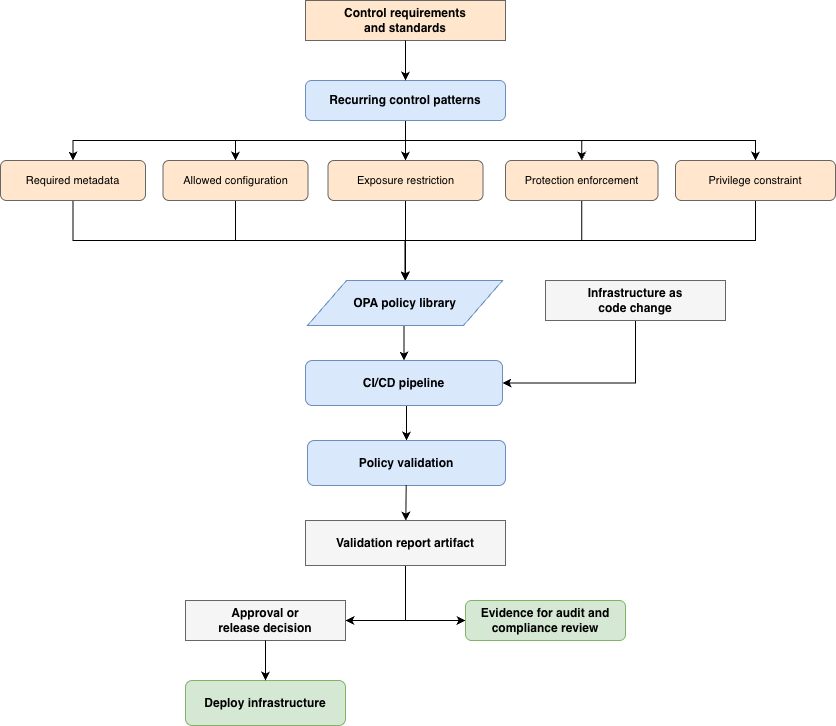
Figure 1: Pattern-based policy as code in a gated delivery workflow
Organize policies around recurring patterns
Teams sometimes build rules one service at a time, which can make policy as code libraries difficult to review and extend as the library grows. Similar control requirements can be expressed differently across repositories, and teams lose a common way to discuss what the policies are enforcing.
A pattern-based approach organizes policies around recurring control intent rather than service-specific checks, as shown in Figure 2. This makes coverage more straightforward to review, explain, and evolve as infrastructure changes.
A practical set of patterns includes:
- Required metadata – for tags and other fields used for ownership, support, cost allocation, and automation.
- Allowed configuration – for approved Regions, accepted deployment boundaries, and other approved settings.
- Exposure restriction – for configurations that make infrastructure more reachable than intended, such as public ingress or internet-facing resources in the wrong environment.
- Protection enforcement – for baseline safeguards such as encryption, logging, or deletion protection.
- Privilege constraint – for AWS Identity and Access Management (IAM) definitions and access patterns that need tighter validation.
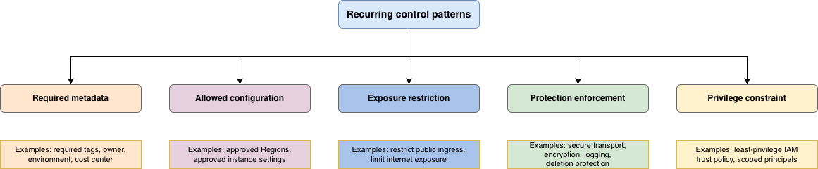
Figure 2: Recurring control patterns used to organize policy as code checks
Where OPA fits in a layered governance model
This post focuses on the preventive layer. You still need runtime controls, drift monitoring, remediation workflows, and compliance reporting. On AWS, AWS Organizations, AWS Control Tower, AWS Config, and AWS Security Hub remain important after resources exist.
OPA fits earlier in the process and validates that infrastructure changes align with expectations. OPA evaluates structured input (HashiCorp Terraform plan JSON) against policy logic. It doesn’t replace AWS governance services that provide organizational guardrails, continuous monitoring, and resource level enforcement after resources exist.
As shown in Figure 3:
- OPA – Checks proposed changes before deployment
- AWS Organizations and Control Tower – Establish organizational guardrails
- AWS Config and Security Hub – Provide visibility and monitoring after resources exist
- Service-level protections – Enforce settings at the resource boundary
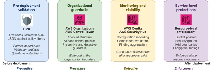
Figure 3: OPA validates changes pre-deployment; AWS services enforce guardrails, monitoring, and controls post-deployment
How to implement policy validation in your CI/CD pipeline
Use the following steps to integrate OPA policy evaluation into your delivery workflow:
Submit a change through a pull request or merge request.
- Run early validation checks such as formatting, syntax validation, and dependency checks.
- Generate a Terraform plan and convert it to JSON format.
- Evaluate the plan (JSON format) against the shared OPA policy library.
- Publish the validation report as an artifact.
- Run additional automated quality checks as needed.
- Use the validation artifact during approval decisions for higher-risk environments.
- Deploy approved changes.
- Continue post-deployment monitoring through AWS-native governance services.
Quality gates provide automated pass or fail results based on defined criteria. Approval gates control whether a change moves into a protected environment. This separation matters—manual approval isn’t the first place where anyone notices missing tags, a disallowed AWS Region, or public ingress. Automated checks identify those issues earlier. OPA belongs in the automated gate layer. Its output also feeds the approval process.
Structure your policy library by control domain and intent
A pattern-based library structure, as shown in the following sample, keeps the policy model closer to how teams talk about controls.
A compliance engineer might describe a requirement as mandatory metadata. A cloud engineer might describe the same requirement as a tagging standard. The pattern structure helps both teams talk about the same thing.
Example 1: Enforce secure transport for Amazon S3
This example demonstrates the protection enforcement pattern for Amazon Simple Storage Service (Amazon S3). The goal is to verify that S3 bucket access is protected in transit by requiring a bucket policy that denies requests when aws:SecureTransport is set to false.
The policy checks two things: whether an S3 bucket policy includes a deny statement that blocks non-encrypted requests, and whether an S3 bucket has any corresponding bucket policy at all. The rule evaluates both create and update actions in the Terraform plan JSON.
This example uses an explicit deny rather than an allow statement for secure transport. An explicit deny overrides allow statements that might exist elsewhere in the policy set, making it the stronger enforcement pattern.
When you adapt this example, decide whether you want to require one exact policy shape or support several equivalent forms of enforcement. A strict rule is more straightforward to reason about, but it might create false positives if teams already use alternate policy structures that achieve the same outcome.
Example 2: Restrict public ingress on sensitive ports
This example implements the exposure restriction pattern. The goal is to identify Amazon Virtual Private Cloud (Amazon VPC) security group configurations that allow public ingress on sensitive ports before those rules are deployed.
The policy evaluates both inline aws_security_group ingress rules and standalone aws_security_group_rule resources, because customer repositories often use both modeling styles.
This example checks directly for public ingress on sensitive ports rather than trying to infer whether later controls might reduce actual exposure. Security group rules are a direct expression of intended network reachability, making them the right place to enforce this pattern early.
When you adapt this example, review which ports to treat as sensitive, whether both IPv4 and IPv6 exposure need checking, and how to handle approved exceptions.
Example 3: Enforce least privilege trust policy for IAM roles
This example implements the privilege constraint pattern for IAM role trust policies. The goal is to identify trust relationships that allow overly broad principals to assume a role. The policy inspects the assume_role_policy document for aws_iam_role resources and looks for wildcard principals in three valid representations: Principal is "*", Principal.AWS is "*", and Principal.AWS is an array containing "*". A wildcard principal allows a broader set of callers than most environments intend to permit. By treating wildcard principals as the prohibited pattern, the rule enforces a safer default and returns a clear result that reviewers can understand quickly.
When you adapt this example, decide what least privilege means for your IAM trust model. The key design choice is whether your policy checks for a single prohibited pattern or validates trust relationships against an approved set of trusted principals and conditions.
AWS Labs provides IAM Policy Autopilot, an open-source Model Context Protocol (MCP) server and command-line tool that helps generate baseline identity-based IAM policies from application code. That is adjacent to the pattern shown here —IAM Policy Autopilot helps with policy generation, while this example focuses on validating whether IAM role trust policies are scoped appropriately in infrastructure changes.
CI/CD implementation examples
The following examples show the same operating model in two common CI/CD systems. The syntax changes, but the sequence stays the same: validate, plan, evaluate policy, retain the artifact, and use the result during promotion and approval. These examples assume OPA is installed in your CI/CD environment, the opa-policies directory contains your policy library, and Terraform is configured with appropriate credentials.
Retain validation artifacts for review and audit support
In mature delivery workflows, policy results don’t disappear into pipeline logs but are retained as validation artifacts. Those artifacts help reviewers decide whether a change is ready for approval, supports exception handling by showing which controls failed and why, and can stay with the change record for later audit discussions. At a minimum, the artifact identifies the change or pipeline run, the evaluated scope, the policy package or version, the checks that ran, and the pass or fail results.
Test the policy model like software
The first few rules are usually straightforward.The real work starts when the library grows and multiple teams depend on it. Testing includes:
- Positive and negative test cases – Each policy has cases that show valid input and cases that show expected failures.
- Regression coverage – Shared helpers need regression coverage.
- Realistic fixtures – Terraform plan fixtures look like real changes rather than tiny made-up samples.
- Impact analysis – When a rule changes, teams can tell quickly what else might be affected.
If developers stop trusting the results, they stop treating policy as a useful mechanism.
A phased approach to rolling out policy checks
You don’t need broad coverage on day one. A phased rollout works better than an all at once enforcement approach.
Phase 1: Assess and pilot
- Start in advisory mode so teams can see results without being blocked.
- Identify two or three high-confidence patterns such as required metadata, approved Regions, or public exposure restrictions.
- Run OPA against existing pipelines and review the output for accuracy.
Phase 2: Begin enforcement
- Enforce the small set of high-confidence patterns after the output is stable and the failures are useful.
- Integrate validation artifacts into your approval workflow.
- Establish ownership and exception handling processes for shared packages.
Phase 3: Operationalize and expand
- Formalize versioning for shared policy packages.
- Expand pattern coverage based on team feedback and organizational priorities.
- Connect pre-deployment validation with post-deployment monitoring through AWS Config, AWS Security Hub, and AWS Organizations.
Conclusion
Policy as code helps narrow the distance between what an organization says it expects and what its delivery system checks. By implementing these OPA patterns in your CI/CD pipelines, you can build a preventive layer that evaluates infrastructure changes before deployment. With a pattern-based library, validation artifacts, and clear ownership, policy as code becomes a repeatable way to help translate control intent into day-to-day delivery, while AWS governance services continue to provide visibility and monitoring after resources exist.
To learn more about policy as code and AWS governance capabilities, see:
- Contact AWS Security Assurance Services – Get help with your compliance engineering journey
- Open Policy Agent Documentation – Read the official OPA documentation and policy language reference
- AWS Security Hub User Guide – Learn how to aggregate and prioritize security findings
- AWS Well-Architected Framework: Security pillar – Review security best practices for your workloads
- AWS Config Developer Guide – Learn how to monitor and record resource configurations
- IAM Policy Autopilot – An open source command line interface (CLI) and MCP server from AWS Labs that helps generate IAM policies
If you have feedback about this post, submit comments in the Comments section below.
Firefox 151.0 released
Post Syndicated from corbet original https://lwn.net/Articles/1073579/
Version
151.0 of the Firefox browser has been released. Significant changes
include the ability to clear and restart a private-browsing session, better
fingerprinting protection, control over the apparent location when using the
Firefox VPN, and more.
JG Wentworth #lastweektonight
Post Syndicated from LastWeekTonight original https://www.youtube.com/shorts/oWLIm0Bs3Rg
A systematic approach to benchmarking SQL processing engines on AWS
Post Syndicated from Anubhav Awasthi original https://aws.amazon.com/blogs/big-data/a-systematic-approach-to-benchmarking-sql-processing-engines-on-aws/
Selecting the right SQL processing solution for large-scale data analytics is a critical decision for organizations. As data volumes grow exponentially, the technology landscape has evolved to offer diverse options for processing and analyzing this information efficiently. This post presents a systematic framework for evaluating and benchmarking SQL processing engines on AWS, using Apache JMeter to conduct practical performance testing at scale.
The AWS analytics ecosystem
AWS offers a rich portfolio of SQL processing solutions to meet various analytical needs:
- Serverless query services – Amazon Athena is a serverless, interactive query service that uses standard SQL to analyze data in Amazon Simple Storage Service (Amazon S3), offering automatic scaling, parallel query execution, and pay-per-query pricing with no infrastructure management required
- Data warehouse solutions – Amazon Redshift offers scalable, high-performance cloud data warehousing with serverless options, zero-ETL integrations, AI-powered query assistance, and seamless machine learning (ML) integration for modern analytics at scale
- Managed open source engines – Amazon EMR supports Apache Spark SQL, Apache Trino (formerly PrestoSQL), and other distributed query frameworks
- Self-managed options – You can deploy open source engines like Apache Spark, Apache Flink, and Trino on Amazon Elastic Kubernetes Service (Amazon EKS) for greater control
- Partner solutions – You can access specialized big data analytics tools through AWS Marketplace
These options are further enhanced by modern open table formats such as Apache Iceberg, Delta Lake, and Apache Hudi, which bring crucial enterprise features like ACID (Atomicity, Consistency, Isolation, and Durability) transactions, schema evolution, and time travel capabilities to data lakes. These SQL processing solutions operate under the AWS Shared Responsibility Model. AWS manages the security of the underlying infrastructure and services, and customers are responsible for secure configuration, access management, and data protection within their testing environments. This division of responsibility remains important when evaluating and benchmarking different SQL engines. Proper security configuration and implementation by customers is essential for maintaining a secure analytics environment.
Evaluation challenges in SQL engine selection
The rich ecosystem of SQL processing options creates significant evaluation challenges. Each SQL engine employs unique architectural approaches and optimization strategies, making direct comparisons complex. Organizations embarking on this evaluation journey face several interconnected obstacles:
- Creating environments that accurately reflect production scenarios
- Developing test datasets that mirror real-world data characteristics and volumes
- Replicating real-world query patterns and concurrency levels
- Maintaining uniform testing conditions across different engine architectures
- Controlling infrastructure expenses throughout the evaluation process
Performance considerations at petabyte scale
When evaluating solutions for petabyte-scale deployments, the complexity intensifies considerably. Several critical factors come into play:
- Resource management – Distributed SQL engines require precise balancing of CPU, memory, and storage resources. Suboptimal resource allocation can lead to query failures and performance degradation, particularly as data volumes grow.
- Data distribution patterns – How data is distributed across partitions or nodes significantly impacts query performance. Data skew can create processing bottlenecks, with some nodes handling disproportionate workloads while others remain underutilized.
- Concurrency handling – High-concurrency environments demand sophisticated workload scheduling and resource isolation mechanisms. The ability to maintain consistent performance under varying concurrent loads becomes a critical differentiator between solutions.
- Meaningful metrics – Performance evaluation at scale requires comprehensive metrics analysis:
- Mean, median, and percentile response times (particularly p90 and p95)
- Query throughput under varying concurrency levels
- Scalability characteristics across diverse workload types
- Resource utilization efficiency during peak loads
Limitations of traditional benchmarks
Although industry-standard benchmarks like TPC-DS and TPC-H provide valuable insights, our experience with multiple customer engagements has shown that tailored, workload-specific testing often reveals performance characteristics not captured by these standardized tests. This is especially true for complex, multi-tenant environments with diverse query patterns. Organizations that complement standard benchmarks with workload-specific testing typically experience shorter proof-of-concept cycles, optimized evaluation costs, and more efficient testing operations. This comprehensive approach helps reduce uncertainty in the final solution selection process.
Prerequisites
Before you dive into the evaluation process, make sure you have the following prerequisites:
- An AWS account with appropriate permissions to create and manage Amazon Elastic Compute Cloud (Amazon EC2) instances and access the SQL engines you plan to benchmark.
- Basic familiarity with AWS services, particularly Amazon EC2 and the SQL engines you intend to evaluate (such as Athena, Amazon Redshift, or Amazon EMR).
- Experience with SQL and data analytics concepts.
- Access to the SQL engines you choose to benchmark. This post assumes you’ve already set up the engines you want to test. For setup instructions, refer to the AWS documentation for each service.
- A dataset suitable for your benchmarking needs. Dataset creation and loading are not covered in this post. Build petabyte-scale synthetic test data with Amazon EMR on EC2 provides prescriptive guidance to generate test datasets at scale. Make sure your test datasets are stored in S3 buckets with encryption enabled (using SSE-KMS or SSE-S3) and that all service connections use TLS for data in transit.
Benefits of Apache JMeter
As organizations scale their analytics workloads to petabyte levels, there is a growing need for a robust, structured approach to SQL query performance testing. Although many organizations develop custom testing frameworks or use various benchmarking tools, these approaches often lack standardization and can be difficult to replicate across different SQL engines. The complexity of modern data architectures, combined with the variety of available SQL processing solutions, demands a systematic evaluation methodology. Apache JMeter emerges as a powerful solution to address this challenge. Though traditionally known for web application testing, JMeter’s extensible architecture and robust feature set make it particularly well-suited for SQL performance testing at scale.JMeter offers several advantages for evaluating SQL engines:
- Support for multiple protocols and connections
- Ability to simulate complex concurrent workloads
- Built-in performance metrics and reporting
- Extensible architecture for custom testing scenarios
- Integration capabilities with continuous integration and continuous delivery (CI/CD) pipelines
Through this proposed framework, which has been validated across multiple customer engagements at petabyte scale, we aim to help organizations make more informed decisions when selecting a SQL processing solution. Our experience working with customers to assess various AWS Analytics services and open source solutions has demonstrated that a systematic evaluation approach significantly reduces proof-of-concept cycles and optimizes resource investments. This framework has helped organizations effectively evaluate services like Athena, Amazon Redshift, and Amazon EMR, alongside open source solutions such as Trino on Amazon EKS, based on their specific workload profiles and performance requirements.With this methodology, organizations can accomplish the following:
- Navigate the complex landscape of large-scale data processing technologies
- Reduce proof-of-concept cycles from months to weeks
- Minimize infrastructure costs during evaluation phases
- Make data-driven decisions about technology selection
- Better align technology choices with business requirements
- Establish repeatable testing patterns for future evaluations
Testing methodology in practice
A successful SQL engine evaluation requires understanding and replicating real-world workload patterns. Our methodology, refined through numerous customer engagements, focuses on comprehensive testing across multiple dimensions while remaining adaptable to specific organizational needs.
Query pattern selection
We begin by selecting representative query patterns that mirror production workloads:
- Aggregation queries that summarize large datasets using operations like SUM, AVG, and COUNT
- Complex join operations that test the engine’s ability to combine data efficiently across multiple tables
- String operations that evaluate text processing capabilities
- Nested queries that assess the engine’s optimization capabilities for complex query structures
A carefully selected set of 8–10 queries typically provides sufficient coverage while keeping the evaluation manageable. These should reflect your actual workload characteristics and business requirements.
Data volume variations
Testing across different data volumes is important for understanding scalability characteristics. We structure our tests around varying data scan ranges:
- Small-scale scans – Queries accessing 1–7 days of data (megabytes to gigabytes)
- Large-scale scans – Queries spanning 14–30 days (terabytes to petabytes)
This approach evaluates both I/O efficiency with large datasets and metadata handling with smaller, frequent queries, helping understand how services like Amazon EMR, Amazon Redshift, or Athena optimize query execution across different access patterns.
Concurrency testing
Real-world analytics environments rarely process single queries in isolation. Our methodology incorporates the following features:
- Progressive concurrency testing starting at lower levels (typically 16, 32, 64, and 128 parallel queries), though these numbers can be adjusted based on your test infrastructure capacity and specific requirements. We recommend starting with smaller concurrency levels and gradually scaling up to understand performance characteristics
- Varied query complexity and frequency (referred to as query weights) to simulate realistic workload distributions. This means some queries are run more often or are more resource-intensive than others, mimicking real-world usage patterns.
- Mixed query patterns running simultaneously to test resource management.
- Consistent execution across different date ranges to evaluate scaling behavior.
This approach is particularly important when evaluating managed services like the workload management capabilities of Amazon Redshift or the resource allocation strategies of Amazon EMR.
Query weight distribution
Production environments typically see varying frequencies of different query types. Our framework incorporates weighted query distribution to simulate real-world scenarios more accurately. In a typical distribution, frequent lightweight queries might represent 60% of the workload, complex analytical queries might comprise 30%, and resource-intensive data processing operations might make up the remaining 10%.This weighted approach makes sure performance testing reflects actual usage patterns rather than artificial benchmarking scenarios. The exact distribution should mirror your organization’s specific workload patterns.
Sequential vs. concurrent testing
Our methodology implements two distinct testing phases:
- Sequential testing – Establishes baseline performance metrics:
- Runs each query type independently across different date ranges
- Runs multiple iterations to provide consistency and identify variability
- Helps understand individual query performance characteristics
- Concurrent testing – Simulates real-world multi-user scenarios:
- Implements weighted query distributions
- Tests different concurrency levels to identify scaling limitations
- Evaluates resource management capabilities of different engines
JMeter efficiently implements both testing phases while maintaining consistent test conditions across SQL engines. Its ability to handle various JDBC connections makes it particularly suitable for testing AWS analytics services.Through this structured approach, organizations can gather comprehensive performance data reflecting their specific use cases, enabling informed SQL engine selection decisions while maintaining core principles of systematic evaluation and realistic workload simulation.
Test plans
To evaluate SQL engines’ performance under varying workloads, we designed two test scenarios: sequential and concurrent execution plans. Each scenario was executed across different data volumes by adjusting the query date range filters to cover 1, 7, 14, and 30 days. These variations simulate typical analytical workloads with progressively increasing data sizes.For sequential runs, each test was treated as a distinct batch, grouping all queries (Query 1 to Query 9) under the same date range—each query will scan data for 1, 7, 14, and 30 days with appropriate date filtering in the query’s where predicate. We used JMeter to capture average query response times for each batch. This configuration was run three times, and the final metrics reflect the average response time across these iterations to ensure reliability and account for environmental variance.Although three iterations provide initial insights, if you observe significant variations in results (typically more than 10% deviation between runs), consider expanding to 10 or more iterations. This additional sampling helps establish statistical significance, identify true performance patterns, and distinguish outliers (beyond three standard deviations) from normal variations. Document any consistent anomalies, because they may indicate important performance or security considerations for your specific environment.The following table shows the sample test plans template for the sequential test plan run.
| Dataset Time Range | Run | Query Weights | ||||||||
| Query 1 | Query 2 | Query 3 | Query 4 | Query 5 | Query 6 | Query 7 | Query 8 | Query 9 | ||
| 1 day | Run 1 | |||||||||
| Run 2 | ||||||||||
| Run 3 | ||||||||||
| Avg | ||||||||||
| 7 days | Run 1 | |||||||||
| Run 2 | ||||||||||
| Run 3 | ||||||||||
| Avg | ||||||||||
| 14 days | Run 1 | |||||||||
| Run 2 | ||||||||||
| Run 3 | ||||||||||
| Avg | ||||||||||
| 30 days | Run 1 | |||||||||
| Run 2 | ||||||||||
| Run 3 | ||||||||||
| Avg | ||||||||||
For the concurrent test plan, we introduced a probabilistic weighted distribution to the queries (Query 1 to Query 9), simulating a more realistic production-like environment where query frequency varies based on business relevance and usage patterns. This added a layer of complexity to better reflect how the SQL engine would perform under real-world concurrent access patterns.The following table shows the sample test plans template for the concurrent test plan run.
| Dataset Time Range | Concurrent Runs | Query Weights | ||||||||
| Query 1 | Query 2 | Query 3 | Query 4 | Query 5 | Query 6 | Query 7 | Query 8 | Query 9 | ||
| 1 days | 8 | 11% | 11% | 11% | 11% | 11% | 11% | 11% | 11% | 11% |
| 16 | 10% | 5% | 24% | 5% | 5% | 5% | 24% | 14% | 10% | |
| 32 | 8% | 3% | 24% | 5% | 5% | 5% | 24% | 16% | 8% | |
| 64 | 7% | 3% | 24% | 6% | 4% | 6% | 26% | 16% | 9% | |
| 128 | 1% | 4% | 19% | 8% | 5% | 7% | 14% | 20% | 22% | |
| *7 days | 8 | 11% | 11% | 11% | 11% | 11% | 11% | 11% | 11% | 11% |
| 16 | 10% | 5% | 24% | 5% | 5% | 5% | 24% | 14% | 10% | |
| 32 | 8% | 3% | 24% | 5% | 5% | 5% | 24% | 16% | 8% | |
| 64 | 7% | 3% | 24% | 6% | 4% | 6% | 26% | 16% | 9% | |
| **128 | 1% | 4% | 19% | 8% | 5% | 7% | 14% | 20% | 22% | |
| 14 days | 8 | 11% | 11% | 11% | 11% | 11% | 11% | 11% | 11% | 11% |
| 16 | 10% | 5% | 24% | 5% | 5% | 5% | 24% | 14% | 10% | |
| 32 | 8% | 3% | 24% | 5% | 5% | 5% | 24% | 16% | 8% | |
| 64 | 7% | 3% | 24% | 6% | 4% | 6% | 26% | 16% | 9% | |
| 128 | 1% | 4% | 19% | 8% | 5% | 7% | 14% | 20% | 22% | |
| 30 days | 8 | 11% | 11% | 11% | 11% | 11% | 11% | 11% | 11% | 11% |
| 16 | 10% | 5% | 24% | 5% | 5% | 5% | 24% | 14% | 10% | |
| 32 | 8% | 3% | 24% | 5% | 5% | 5% | 24% | 16% | 8% | |
| 64 | 7% | 3% | 24% | 6% | 4% | 6% | 26% | 16% | 9% | |
| 128 | 1% | 4% | 19% | 8% | 5% | 7% | 14% | 20% | 22% | |
For example, for configuration of *7 days concurrent run with **128 concurrency, the proposed configuration distributes Query 1 to Query 9 with appropriate weighted submissions such that Query 9 is executed the greatest number of times in the overall 128 executions submitted across all 9 queries for this run.
JMeter setup
To begin, you must set up JMeter on a machine that can handle the desired test load. An EC2 instance is a flexible and cost-effective option. Choose an instance type with sufficient vCPUs to support your maximum planned concurrency. For example, a c6i.4xlarge or higher is typically suitable for moderate to high throughput testing scenarios. For the operating system, you might choose Amazon Linux, which is optimized for AWS. For production-grade testing environments, deploy the JMeter EC2 instance in a private subnet of a virtual private cloud (VPC) with appropriate security groups that allow only required connections. This network isolation helps maintain security while executing performance tests. Consider using Amazon Virtual Private Cloud (Amazon VPC) endpoints for secure access to AWS services.
After the instance is provisioned, install Java (Java 17 LTS or Java 21 LTS) and download the latest version of JMeter. Be sure to configure the system with appropriate JVM options to allocate sufficient heap memory for large-scale test executions. Refer to Getting Started to learn more.
JMeter concepts
Before you create test plans in JMeter, it’s important to understand a few foundational concepts that influence how your test plan behaves—such as thread groups, user-defined variables, and JDBC connection. These components enable the simulation of real-world query loads, including concurrency and pacing.
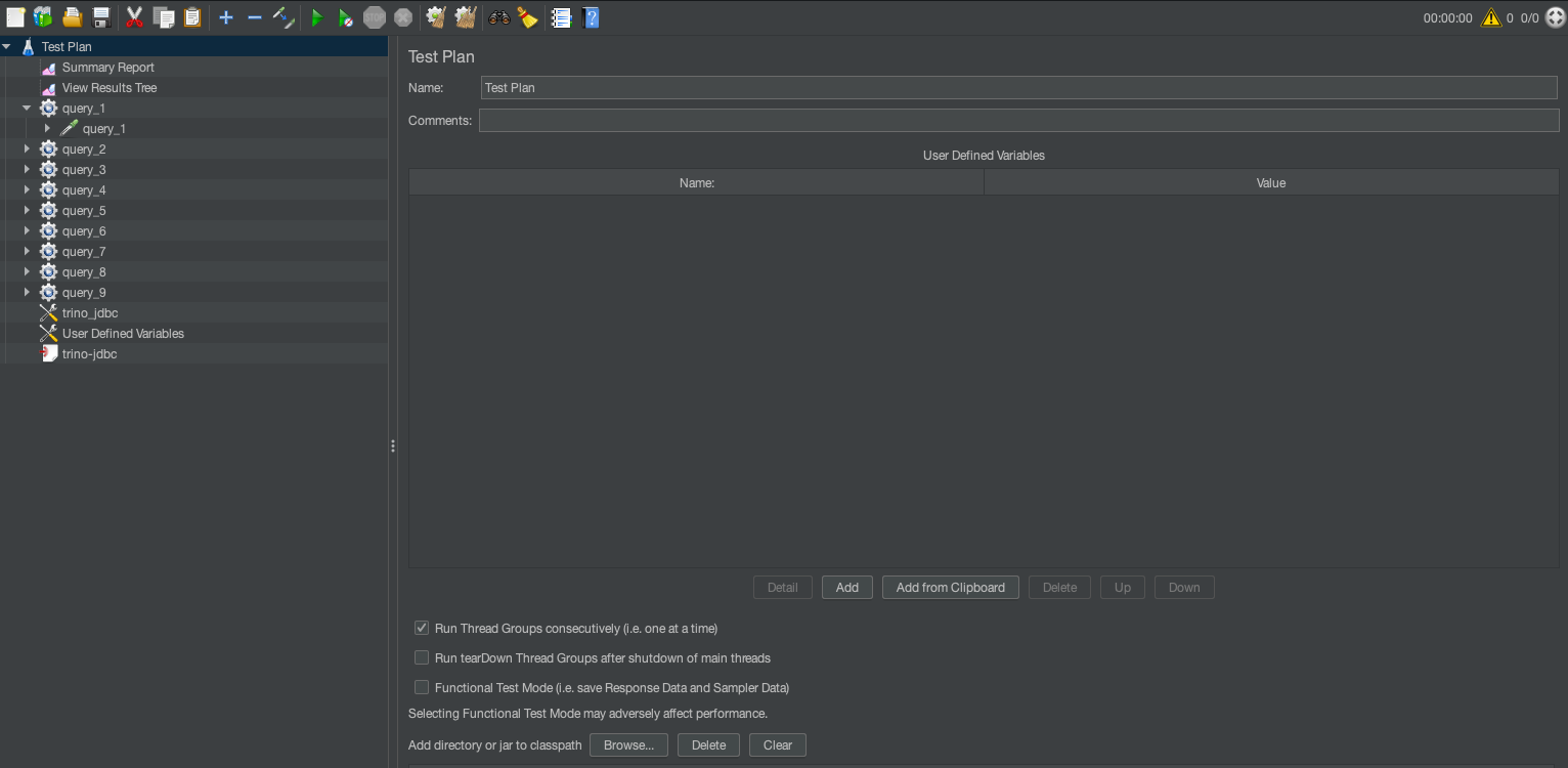
Test plans
The test plan is the top-level container for a JMeter test. It defines the overall testing strategy, including the queries to execute, their parameters, and the concurrent user behavior. These plans are represented as jmx files that can then be used for CLI-based execution. JMeter supports both GUI and CLI modes. It is highly recommended that you use the JMeter GUI primarily for creating test plans as jmx, and use the CLI for large load tests. You can also run thread groups consecutively for sequential execution. The default behavior is to run all thread groups in parallel suited for concurrent execution. Refer to Building a Test Plan to learn more about options available with test plans.
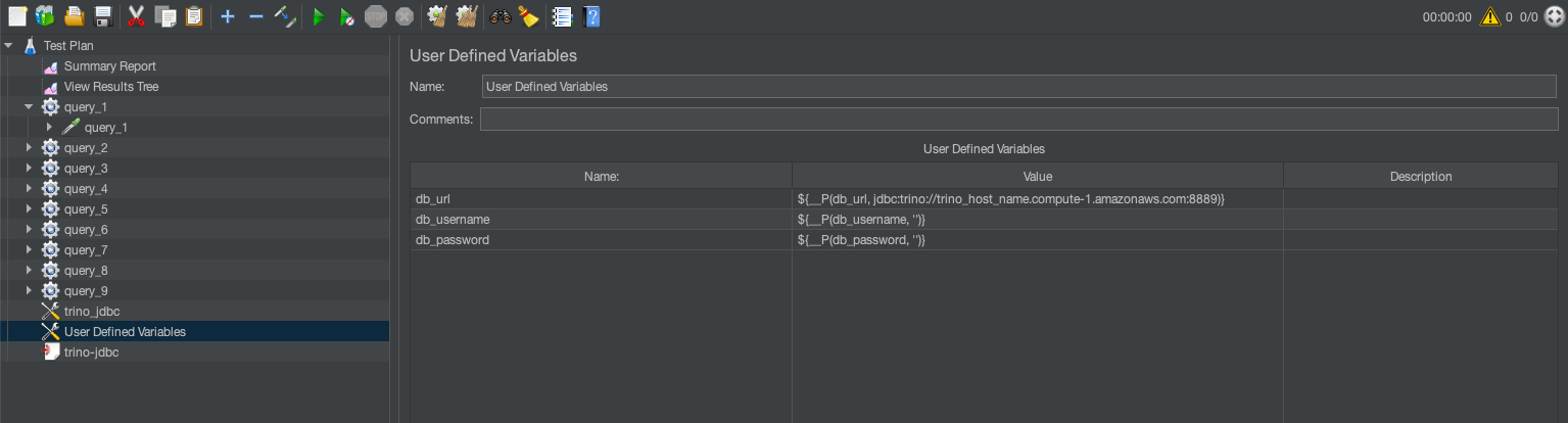
User-defined variables
User-defined variables are global parameters that you can reuse throughout the test plan. They are helpful for defining database credentials, server URLs, or query parameters. For example:DB_URL=jdbc:trino://trino-cluster.example.com:8889?SSL=true #Enable SSL/TLS
You can configure authentication (user name and password) through your organization’s approved methods, such as AWS Secrets Manager (see Move hardcoded secrets to AWS Secrets Manager) AWS Identity and Access Management (IAM) roles, or other secure credential management systems.
Thread groups
A thread group represents a group of virtual users (threads) executing test actions. Each thread simulates a single user sending requests to the SQL engine. This can be used to simulate concurrent runs. For example, in the preceding template, Query 3 has 19% weightage across 128 runs. This means .19*128=25 total runs, so we set the thread group to 25.
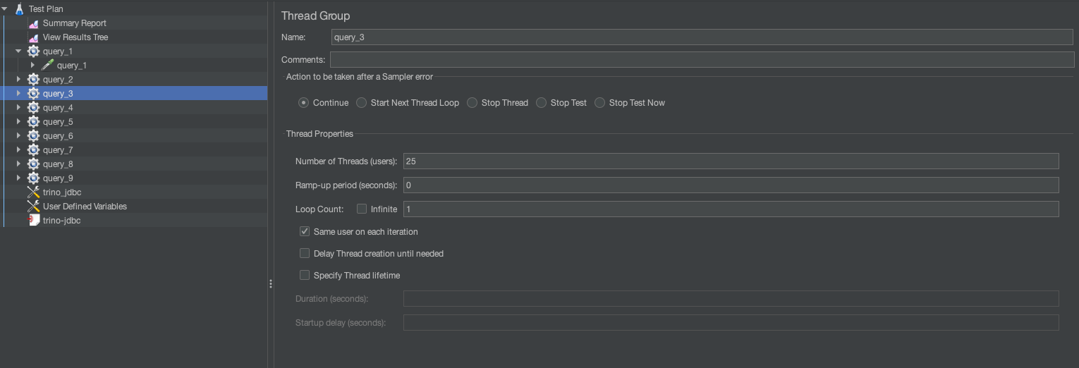
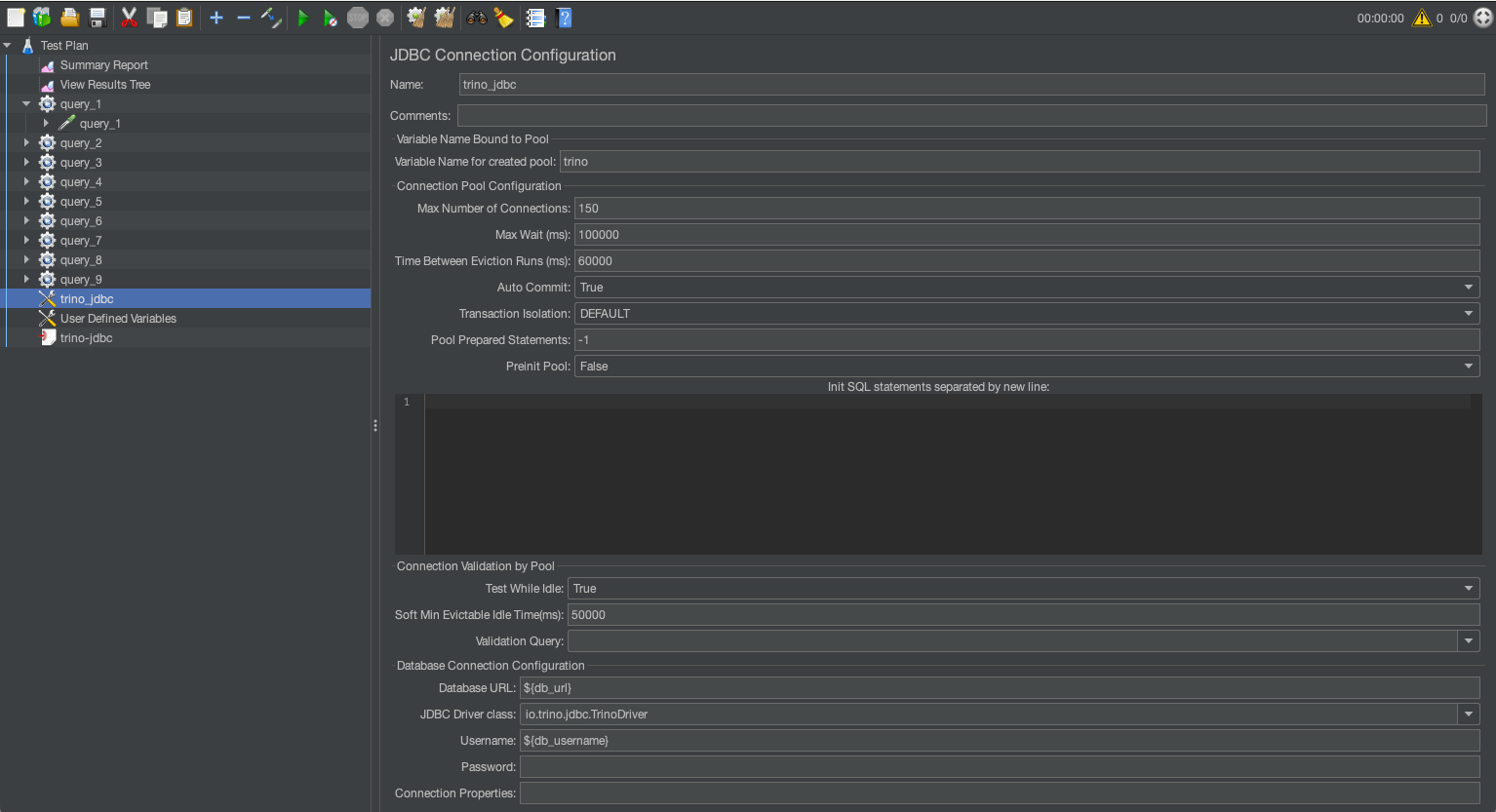
JDBC connection configuration
JDBC connection configuration sets up the database connection for the test. It specifies the database URL, driver, and credentials required for executing SQL queries. Key fields to configure are database URL and JDBC driver class. The following table summarizes the different configuration settings.
| SQL Engine | JDBC Driver | JDBC Driver Class |
| Trino on EMR | trino-jdbc-<trino_version>-amzn-0.jar |
io.trino.jdbc.TrinoDriver |
| Athena | Athena JDBC 3.x driver | com.amazon.athena.jdbc.AthenaDriver |
| Amazon Redshift | Amazon Redshift JDBC driver | com.amazon.redshift.jdbc.Driver |
| Trino on EKS | Trino JDBC driver | io.trino.jdbc.TrinoDriver |
JDBC requests
The JDBC request executes SQL queries against the database using the configuration defined in the JDBC connection configuration.
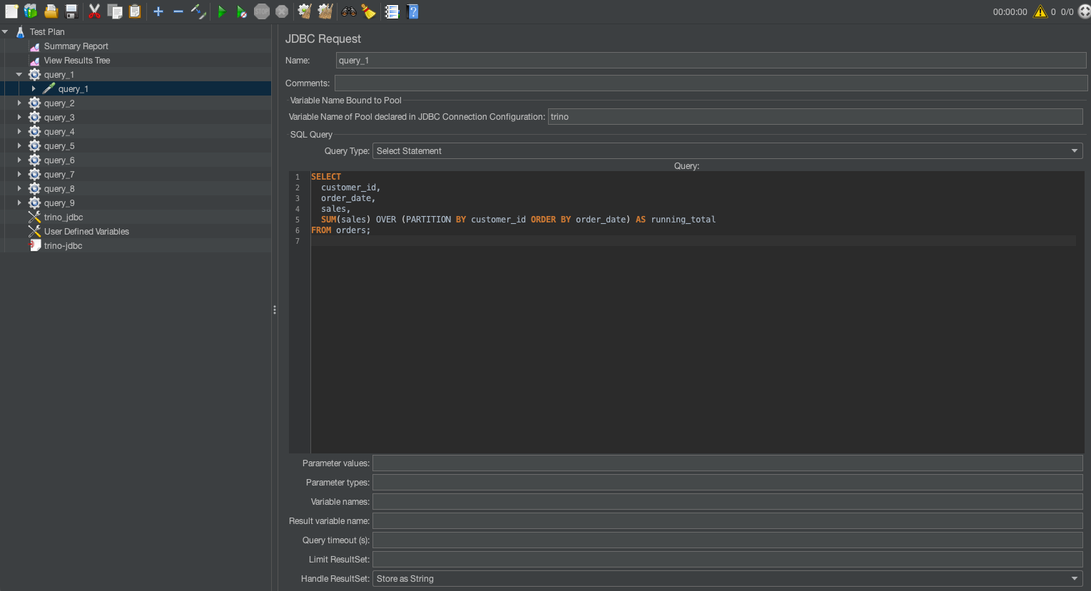
For example, following command runs the JMeter in CLI mode:
The output folder will contain an HTML report with different statistics. The following screenshot illustrates 128 concurrent runs.
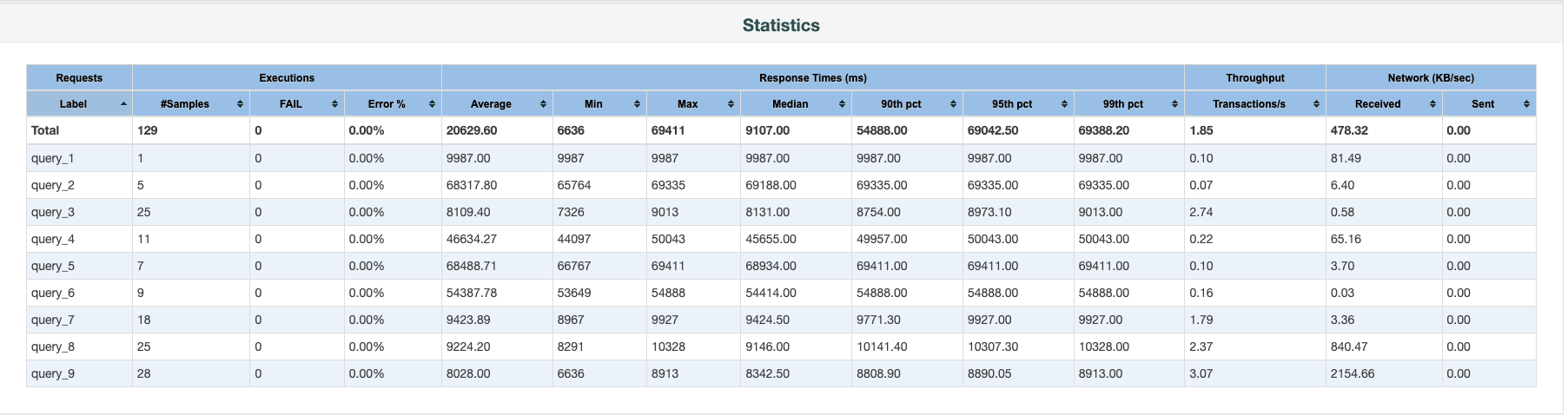
Monitoring and logging
For comprehensive visibility and audit requirements, enable AWS CloudTrail logging, VPC Flow Logs, and service-specific logs (like Amazon S3 access logs). These logs can be centralized in Amazon CloudWatch Logs for monitoring and analysis. This provides proper audit trails while evaluating different SQL engines and helps track access patterns and potential security events.
Post-test steps
After running your JMeter tests, proceed with the following steps:
- Review the HTML report’s key metrics, including response times, throughput, and error rates across different query types and concurrency levels.
- Run identical test plans across your candidate SQL engines for direct performance comparison.
- Refine your test plans based on initial findings, focusing on areas where performance differences are significant.
- Factor in the cost implications alongside performance metrics to make a balanced decision.
These steps can help you systematically evaluate and select the most suitable SQL engine for your analytics workloads.
Resources
In the preceding steps, we walked through a UI-based setup for JMeter along with test plans. We have created a few sample JMeter test plans for both sequential and concurrent runs along with sample test reports. You can modify the plans to fit your needs.
- JMeter sample report
- JMeter test plan for sequential run
- JMeter test plan for concurrent run
Clean up
After you complete your benchmarking process, clean up the resources to avoid unnecessary costs:
- Stop or delete the EC2 instances used for running JMeter.
- Depending on which SQL engines you used for testing, clean up active resources.
- Review your AWS Management Console to confirm no active resources remain.
- If you created test datasets in Amazon S3 or other storage services specifically for this benchmarking, consider deleting them if they’re no longer needed.
- Although JMeter test plans and results don’t incur AWS costs, organize or delete local files as needed for your record-keeping.
Summary
Selecting the right SQL processing solution for large-scale analytics demands a systematic, data-driven approach. Our JMeter framework can help organizations effectively evaluate different SQL engines by simulating real-world workload patterns across various query types, data volumes, and concurrency levels. This methodology reduces proof-of-concept cycles and provides insights beyond traditional benchmarks, helping you assess managed AWS services like Athena and Amazon Redshift and open source solutions on Amazon EKS.
About the authors
GPUs Are Only Half the Equation
Post Syndicated from David Johnson original https://www.backblaze.com/blog/gpus-are-only-half-the-equation/

AI cloud platforms have spent the last few years competing on GPU availability, interconnects, and cluster performance. That makes sense. GPUs are the engine of AI infrastructure, and demand for them has been relentless.
But a GPU can only work as fast as the data pipeline feeding it.
Think of it like a fleet of race cars. You can have the best cars on the track, the fastest pit crew, and a perfect race strategy. But if the fuel lines supplying the pit tanks can’t move gasoline fast enough, the cars are going to sit there waiting.
The cars are not the problem. The fuel supply system is.
The same thing happens in AI infrastructure. GPUs rely on high-performance flash storage when training models or running inference. But before data can be served from that flash tier, it often needs to move from durable object storage into the performance layer. If that upstream object storage layer can’t deliver data quickly and consistently, the entire pipeline slows down.
That’s why GPU availability is only half the equation. The other half is the data supply architecture that keeps those GPUs working.
The hidden bottleneck in AI infrastructure
AI workloads move a lot of data, constantly. Training datasets need to be staged and prepared so jobs can access them quickly. Model checkpoints, artifacts, embeddings, and intermediate outputs need to be written back for durability and reuse. Inference pipelines generate their own steady stream of reads and writes as models serve predictions and capture outputs.
All of that activity puts pressure on the storage and networking layers underneath the AI platform.
The bottleneck usually does not come from one obvious failure. Instead, it builds from a few things happening at once:
- Data retrieval slows down under load.
- Network paths become congested.
- Request overhead compounds at dataset scale.
- I/O behavior becomes less predictable as concurrency increases.
Individually, each of these may seem manageable. Together, they can quietly limit how efficiently AI infrastructure runs.
And the problem gets more visible as platforms scale. A handful of GPUs might be fine, while dozens or hundreds of GPUs create a very different demand profile. The upstream storage layer has to sustain much higher aggregate throughput while also absorbing frequent checkpoint and artifact writes.
Adding more GPUs increases potential compute capacity. But it also increases the rate at which data has to move.
Without enough throughput from the upstream data layer, more compute does not automatically translate into more performance.
Idle GPUs are expensive GPUs
When GPUs wait on data, the impact is both technical and financial.
First, idle GPUs waste compute capacity. GPU time is expensive, and AI workloads are designed to keep those processors busy. When the data pipeline can’t keep up, organizations end up paying for compute that is not being fully used.
Second, data delays slow development. Training runs take longer. Clusters stay reserved for more time. Teams wait longer to evaluate results. Even small drops in utilization can raise the cost of AI work because each run takes longer to finish.
Over time, that means slower iteration, delayed experiments, and longer paths to new models and features.
For AI cloud platforms, the risk is even bigger. Customers judge the platform by outcomes: how quickly jobs start, how consistently workloads run, and whether performance scales as expected. If jobs take longer than expected or results vary from run to run, customers may assume the GPUs are the issue.
But the real problem may be that the data pipeline can’t deliver data fast enough.
AI changes what object storage needs to do
Object storage has traditionally been evaluated around durability, scalability, cost, and general-purpose cloud performance. Those still matter, and AI infrastructure adds a new requirement: sustained data movement.
AI workloads require an object storage layer that can continuously supply downstream performance tiers under real-world load.
That means object storage needs to:
- Sustain high aggregate throughput, not just short bursts.
- Deliver predictable performance under continuous data movement.
- Absorb large checkpoint and artifact writes.
- Quickly rehydrate data when needed.
Many traditional object storage architectures were not built for this kind of steady, high-volume supply model. They can perform well for archival workloads, backups, and general-purpose applications, but AI introduces sustained pressure that exposes architectural limits.
The result is rarely a dramatic failure. More often, it looks like variability. Performance fluctuates under load. Scaling becomes harder to predict. GPU clusters wait on data more often than they should.
That variability becomes a competitive problem.
For AI clouds, storage is now part of the product experience
GPU availability is becoming table stakes. What separates platforms is not just how many GPUs they advertise, but how reliably those GPUs translate into real-world AI performance and productivity.
We said that customers care about outcomes. They want models to train faster. They want workloads to stay stable as they scale. They want infrastructure that helps them iterate quickly instead of introducing another bottleneck.
That means the upstream data layer has become performance infrastructure.
The storage layer also shapes the customer experience. If storage feels disconnected, complicated, or bolted on, customers notice. If it is native, branded, performant, and easy to consume, it strengthens the platform.
That is where B2 Neo comes in.
B2 Neo: Storage built to keep AI workloads moving
Backblaze B2 Neo gives platforms a high-throughput, white-label object storage backbone designed to support AI workloads at production scale.
It is S3-compatible, engineered for sustained throughput, and built to supply high-performance flash tiers without forcing providers to build and operate complex storage infrastructure in-house.
With B2 Neo, AI cloud platforms can offer object storage as a native extension of their own platform, including branded endpoints, partner-controlled pricing, and API-driven provisioning. That gives providers a new branded revenue stream while keeping the customer experience centered on their own platform.
B2 Neo also supports private connectivity options, helping create dedicated data paths that reduce shared network contention and improve predictability for demanding workloads. Backblaze has positioned the platform for high-throughput use cases, including up to 1Tbps aggregate throughput for AI and media workloads.
For platforms, that means storage becomes less of a build-vs-buy distraction and more of a platform advantage.
What AI clouds gain
When the data supply layer can keep up, GPU infrastructure becomes more effective.
Neocloud platforms can improve GPU utilization by reducing the time clusters spend waiting on data. AI teams can iterate faster because training runs and experiments move through the pipeline more efficiently. Platform performance becomes more predictable as datasets grow and clusters scale.
And operationally, neoclouds avoid the burden of building, scaling, and maintaining a large object storage system themselves.
That matters because every engineering cycle spent building commodity infrastructure is a cycle not spent improving the core compute platform, customer experience, orchestration layer, or AI-specific tooling.
The bottom line
AI clouds are winning because they give builders access to the compute resources they need. But compute alone is not enough.
A GPU cluster is only as useful as the data pipeline that keeps it fed.
As AI workloads scale, the storage layer becomes part of the performance story. The neoclouds that solve the data throughput problem will be better positioned to deliver consistent customer outcomes, improve GPU utilization, and turn storage into a native part of the platform experience.
GPU availability is only half the equation; Backblaze delivers the other half.Interested in learning how Backblaze supports AI cloud platforms? Explore B2 Neo or reach out to start a technical and strategic conversation.
The post GPUs Are Only Half the Equation appeared first on Backblaze Blog | Cloud Storage & Cloud Backup
Build petabyte-scale synthetic test data with Amazon EMR on EC2
Post Syndicated from Anubhav Awasthi original https://aws.amazon.com/blogs/big-data/build-petabyte-scale-synthetic-test-data-with-amazon-emr-on-ec2/
As you scale your data systems, you face a challenge: how to test thoroughly without putting customer data at risk. Using production data for testing can expose sensitive customer information to unauthorized access or breaches. For customers in regulated industries like finance and healthcare, this risk isn’t only a concern. It’s unacceptable. A data breach during testing could compromise their privacy, damage their trust, and expose organizations to significant compliance penalties. Synthetic test data solves this problem by generating artificial datasets that replicate the structure and patterns of real data without containing any actual customer information. This approach means you can test performance, validate data pipelines, and develop new features while ensuring that customer data remains protected and compliance requirements are met.
As data volumes grow from terabytes to petabytes, the architecture for generating synthetic data must evolve to meet increasing demands for scale, performance, and data quality. In this post, we show how you can build a scalable synthetic data generation solution using Amazon EMR, Apache Spark, and the Faker library.
The challenge of synthetic data generation
Traditional benchmark datasets like TPC-DS provide standardized schemas and predetermined data volumes for consistent testing environments across different systems. However, they fall short in meeting real-world testing requirements. These benchmarks don’t capture industry-specific patterns or the complex relationships found in actual production data. Their rigid schemas and simplified distributions fail to reflect business requirements, and scaling them while maintaining data consistency proves difficult. Perhaps most critically, generating massive datasets with traditional approaches requires specialized architectures to avoid proportional increases in compute costs and time.
Requirements for production-grade synthetic data
Effective workload validation demands synthetic data that mirrors production distributions while maintaining referential integrity across related tables and entities. The generation process must scale horizontally to accommodate growing data volumes while delivering deterministic results. Given identical input parameters, the system should produce the same dataset across multiple runs, supporting consistent testing cycles and comparative analysis.
Beyond technical requirements, synthetic data addresses compliance needs by minimizing exposure of personally identifiable information (PII) and protected health information (PHI) in non-production environments. This approach satisfies GDPR, HIPAA, and CCPA requirements while supporting secure cross-border data transfer, regular stress testing without compromising sensitive information, and providing an audit-friendly alternative to data masking that preserves analytical properties.
Solution overview
Architecting a synthetic data generation system that scales from terabytes to petabytes requires balancing several competing demands: the system must scale horizontally while maintaining data quality, generate large volumes efficiently, manage compute and storage resources cost-effectively, and support various schemas and output formats.
Our architecture addresses these challenges through four core components. Apache Spark on Amazon EMR provides the distributed computing framework necessary for large-scale generation. The Faker library offers synthetic data generation functions that integrate with Spark. Amazon Simple Storage Service (Amazon S3) with Apache Iceberg serves as the storage layer. We chose Iceberg for its schema and partition evolution capabilities without data rewrites, atomic transactions for consistency, precise time travel features for reproducible testing, and optimized performance at extreme scale. Amazon EMR handles dynamic resource allocation and cluster management.
The following diagram illustrates the solution architecture.
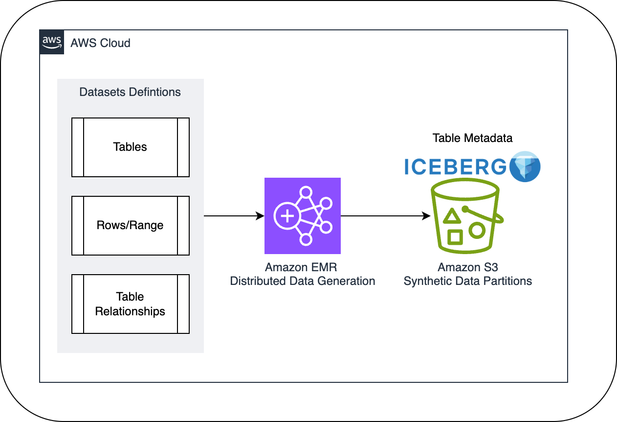
Synthetic data generation at scale with Amazon EMR
Amazon EMR emerges as a particularly powerful solution for this use case, offering several advantages that directly address our requirements. It facilitates scaling of compute resources through instance fleets and Spot Instances, which can reduce costs by up to 90% compared to On-Demand pricing. The service provides built-in performance optimization for Spark applications with real-time monitoring through Amazon CloudWatch integration.
The managed infrastructure reduces operational overhead by handling the underlying Spark ecosystem and cluster lifecycle, while still providing control over scaling policies, instance types, and configurations. Integration with Amazon S3, AWS Glue, and Amazon Athena facilitates end-to-end data generation and testing workflows. Support for multiple programming languages and notebooks provides flexibility in implementing generation logic tailored to specific testing scenarios.
The synthetic data generation process follows a systematic approach designed for efficiency and scalability, as illustrated in the following diagram.

Although synthetic data generation isn’t a sensitive workload, it’s important to maintain robust security throughout the data generation process. Amazon EMR provides security features that align with organizational compliance requirements.
For comprehensive security guidance specific to Amazon EMR deployments, refer to Security in Amazon EMR. The solution follows the AWS Shared Responsibility Model, where AWS manages the security of the cloud infrastructure, and customers maintain responsibility for data security, access management, and compliance controls in the cloud. Specifically for synthetic data generation workloads, AWS manages the security of the underlying Amazon EMR infrastructure, network, and service operations, and customers implement appropriate security controls for their data generation pipelines. Consider the following key areas:
- Data protection – Enable encryption at rest and in transit using Amazon EMR security configurations, including Amazon S3 encryption and TLS certificates for inter-node communication.
- Network security – Deploy Amazon EMR clusters in private subnets with security groups following least privilege, and enable the Amazon EMR block public access feature.
- Access control – Implement AWS Identity and Access Management (IAM) roles with least privilege for Amazon EMR service roles, Amazon Elastic Compute Cloud (Amazon EC2) instance profiles, and runtime roles to isolate job access. Fine-grained table-level and column-level permissions can be controlled using AWS Lake Formation. Additional authentication options are available using Kerberos and LDAP.
Optimize Faker for petabyte-scale data generation
When generating synthetic data at petabyte scale, using Faker’s implementations can quickly lead to performance bottlenecks. To overcome these limitations, adopt a combination of different optimization approaches instead of the default setup. Some of the approaches we adopted in this scenario are discussed in this section.
Faker instance pooling
The following code creates multiple Faker instances to avoid contention when generating data in parallel:
Consistent seed management
The following code provides reproducible data generation across distributed executors:
Random access to Faker pool
The following code distributes load across multiple Faker instances to reduce contention:
Broadcast variables for reference data
The following code efficiently distributes reference data to all executors:
Batch generation of synthetic data
The following code generates fake data in batches rather than one-by-one:
ThreadPoolExecutor for parallel processing
The following code uses Python’s threading for parallel operations within executors:
Optimize Amazon EMR and Spark
When processing massive datasets with Spark on Amazon EMR, carefully tuning configurations can substantially enhance performance beyond the standard settings. In this section, we discuss ways to optimize the execution environment, so you can efficiently handle petabyte-scale workloads with synthetic data generation. By strategically using Spark’s advanced features and configuring Amazon EMR for your specific use case, you can improve throughput, reduce processing time, and maximize resource utilization.
Arrow configuration
The following code enables Apache Arrow for efficient data transfer between Python and JVM. The default value is false.
Enable this configuration when your PySpark application frequently converts data between Python and JVM, especially for large DataFrames or when using Pandas operations. Keep this setting disabled for pure Spark SQL workloads or when memory is constrained.
This optimization is most effective in the following scenarios:
- When processing large-scale datasets that require frequent conversion between Python and JVM.
- In a PySpark application where large DataFrame operations and Pandas integration are needed.
- With data science workloads that combine Python UDFs with Spark SQL operations.
Consider the following trade-offs:
- Arrow maintains in-memory columnar format, resulting in increased memory consumption.
- Not all data types are fully supported in older versions of Spark.
- It might introduce overhead for very small datasets where conversion costs outweigh the benefits.
Adaptive query execution
The following code allows Spark to dynamically optimize query execution plans. The default value is true in Spark 3.2 and later, and false in earlier versions.
This optimization is generally recommended to keep enabled for most workloads. Consider disabling only when you have highly optimized, predictable queries where the adaptive overhead isn’t beneficial, or when troubleshooting query performance issues.
This optimization is most effective in the following scenarios:
- Complex join operations with unknown or skewed data distributions.
- Multi-stage queries where initial plans might be suboptimal.
- When processing data with changing characteristics over time.
Consider the following trade-offs:
- You may experience additional overhead during the query planning phase.
- You might occasionally choose suboptimal plans for certain edge cases.
Parallelism configuration
The following code sets appropriate parallelism for distributed data processing based on the volume of data you’re generating. The default value for spark.default.parallelism is the total number of cores on all executor nodes or 2, whichever larger. The default value for spark.sql.shuffle.partitions is 200.
Adjust this configuration when the default of 200 shuffle partitions creates too many small tasks (increase data volume) or too few large tasks (decrease for smaller datasets). Generally, aim for partition sizes of 100–200 MB. Modify default.parallelism when your RDD operations need different parallelism than the CPU-based default.
This optimization is most effective in the following scenarios:
- When generating consistent volumes of synthetic data across multiple runs.
- When you have predictable resource requirements.
- When you need to precisely control executor utilization.
Consider the following trade-offs:
- Static configuration might not adapt well to varying data volumes.
- Too many partitions can lead to task scheduling overhead.
- Too few partitions might cause memory pressure on executors.
Memory management
The following code optimizes memory allocation for execution and storage. The default value for spark.memory.fraction is 0.6, and for spark.memory.storageFraction is 0.5.
Increase memory.fraction from 0.6 to 0.8 when your workload is memory-intensive and you’re not using the JVM heap for other purposes. Adjust storageFraction based on your caching vs. execution memory needs. Decrease to 0.3 if you do minimal caching but have complex computations, and increase to 0.7 or higher for cache-heavy workloads.
This optimization is most effective in the following scenarios:
- Workloads that are memory-intensive and need fine-grained control.
- Workloads that balance between execution memory and cached data.
- During synthetic data generation that has many interdependent fields.
Consider the following trade-offs:
- Incorrect memory configuration can lead to frequent spills to disk or out-of-memory (OOM) errors.
- You might need to change the configuration to suit different workload characteristics.
- The settings must be monitored and tuned for optimal performance.
Limited Python UDF usage
The following code uses Spark’s built-in functions where possible instead of Python user-defined functions (UDFs). No additional configuration is needed. This is a coding practice.
We recommend using Spark functions over Python UDFs when the same functionality can be achieved. Use Python UDFs only when complex business logic can’t be expressed using Spark’s built-in functions, or when integrating with specialized Python libraries.
This optimization is most effective in the following scenarios:
- Simple transformations that can be performed using Spark functions.
- High-throughput workloads where serialization overhead needs to be minimized.
Consider the following trade-offs:
- This approach is less flexible compared to customer Python-based transformations or functions.
- You might need to use complex expressions to accomplish certain data patterns.
- There is a potential learning curve to familiarize yourself with Spark functions.
DataFrame caching
The following code caches frequently used DataFrames to avoid regenerating data. The default behavior doesn’t use caching. DataFrames are recomputed on each action.
Use this optimization to cache DataFrames that are accessed multiple times in your application. Monitor memory usage and use MEMORY_AND_DISK storage level for large DataFrames. Uncache DataFrames when they’re no longer needed to free memory.
This optimization is most effective in the following scenarios:
- When reusing reference data across multiple operations (can result in performance gains).
- For workloads where the same data is processed on multiple occasions.
Consider the following trade-offs:
- Too much caching might lead to memory process.
- Planning is required to manage cache in environments where memory is scarce.
Optimal partitioning
By default, Spark determines partitioning based on input data and previous operations. The following code makes sure data is properly distributed across executors:
Use repartition() when you need to increase partitions for better parallelism or support even data distribution. Use coalesce() when reducing partitions to avoid small files. Generally, target 100–200 MB per partition for optimal performance.
This optimization is most effective in the following scenarios:
- When controlling data distribution and avoiding data skew is very important.
- Before executing an expensive operation that will benefit from balanced data distribution.
- When optimizing downstream consumption use cases.
Consider the following trade-offs:
- This option is more expensive than
coalesce(). For large datasets,repartition()can lead to large shuffle. - The approach requires trial and experimentation to determine the optimal partition count.
- There is no “one-size-fits-all” setting. Different applications or operations might gain performance with different partitioning.
Partition-aware writing
By default, data is written without partitioning. The following code organizes data for efficient storage and retrieval:
Partition data when you have predictable query patterns that filter on specific columns. Choose partition columns that are frequently used in WHERE clauses and have reasonable cardinality (avoid too many small partitions or too few large ones).
This optimization offers the following benefits:
- Allows for highly parallel write operation across multiple executors.
- Organizes the data that is close to real-world production data.
- Allows for partition pruning when querying the data.
Consider the following trade-offs:
- Excess partitioning or too fine-grained partitioning might result in small files.
- It might result in data skew because of hot partitions.
- You might encounter storage and metadata overhead because of excessive partitions.
Best practices
Through our journey from terabytes to petabytes, we’ve identified several best practices:
- Begin with a modest dataset and incrementally scale, allowing for identification of bottlenecks at each stage.
- Implement robust data validation checks to confirm synthetic data maintains expected properties at scale.
- Regularly review and adjust Amazon EMR configurations, using Spot Instances and right-sizing clusters.
- Develop parameterized job scripts that can adjust data volume, complexity, and cluster resources dynamically.
- Design your synthetic data schema and generation logic to quickly accommodate new fields or changing distributions over time.
Conclusion
Our journey from terabytes to petabytes of synthetic data generation demonstrates how Amazon EMR, combined with Spark and Faker, can effectively address large-scale testing needs. The architecture we explored in this post scales to meet demanding data generation requirements while maintaining data quality and cost-efficiency.
We showed how starting with a solid foundation at terabyte scale, then gradually expanding through Amazon EMR managed services and Spot Instances, helps organizations build robust synthetic data pipelines. The combination of efficient data generation techniques, proper validation, and continuous monitoring provides reliable results at scale.
To begin implementing your own synthetic data generation system, start small, test thoroughly, and scale incrementally. For implementation guidance, refer to Generate production-grade synthetic data at petabyte-scale using Apache Spark and Faker on Amazon EMR.
About the authors
Meet Amazon Redshift RG – AWS Graviton-based instances with an integrated data lake query engine delivering up to 2.4x better performance at 30% lower price than RA3
Post Syndicated from Ankit Sahu original https://aws.amazon.com/blogs/big-data/meet-amazon-redshift-rg-aws-graviton-based-instances-with-an-integrated-data-lake-query-engine-delivering-up-to-2-4x-better-performance-at-30-lower-price-than-ra3/
On May 12, 2026, we announced the general availability of Amazon Redshift RG instances, powered by AWS Graviton processors. RG instances are up to 2.2x as fast for data warehouse workloads and up to 2.4x as fast for data lake workloads, all at 30% lower price per vCPU compared to RA3 instances. RG instances support all data lake formats supported by RA3 and eliminate Amazon Redshift Spectrum’s per-TB scanning charges. RG instances feature a custom-built integrated vectorized query engine, making them a more performant and cost-effective foundation for unified analytics.
We are launching with two instance sizes: rg.xlarge and rg.4xlarge, with additional sizes coming later this year.
Why we built this
RG instances bring the power of AWS Graviton processors to Amazon Redshift Provisioned clusters for the first time, paired with a purpose-built vectorized query engine. By combining Graviton’s superior price-performance with the latest Amazon Redshift innovations, RG instances deliver a step-change improvement across two dimensions: significantly lower cost and meaningfully faster performance for both warehouse and data lake workloads using Apache Iceberg and Apache Parquet. We built RG to help you avoid choosing between performance and economics. Graviton costs less to operate, and we’re passing that benefit to you while simultaneously raising the performance bar. Equally important, we designed RG to maintain full feature parity with RA3, so you can modernize your existing clusters without rearchitecting workloads or sacrificing capabilities you depend on today.
This combination is also increasingly critical for agentic artificial intelligence (AI) workloads. AI agents operating at scale generate a new class of analytics demand: high volumes of unique, unpredictable queries that require fast, low-latency responses to keep agents productive. Traditional price-performance ratios make running these workloads at scale cost-prohibitive. RG instances address this head-on. Lower per-vCPU pricing makes sustained high-query volumes economically viable, while improved query performance makes sure agents get answers fast enough to remain effective. Together, this provides the foundation for AI-driven analytics at the scale and economics that agentic workloads demand.
What’s new
RG instances: Better performance, lower cost
RG instances run on AWS Graviton, Amazon’s custom-designed cloud processor built from the ground up to deliver superior price-performance and energy efficiency. This translates directly into RG instances offering more compute cores, higher memory bandwidth, and lower inter-process communication latency compared to RA3, with performance improvements across warehouse, data lake, and mixed workloads.
Graviton costs less to operate, and we’re passing that benefit directly to you. RG instances are priced at a 30% lower cost per vCPU compared to RA3. Reserved Instance pricing follows the same model, making RG Reserved Instances equally 30% less costly than RA3. For pricing details, visit the Amazon Redshift pricing page.
Performance results
RG instances deliver faster, more efficient analytics across your most demanding warehouse and data lake workloads, whether you’re querying structured data in Amazon Redshift Managed Storage (RMS), running analytics over Iceberg tables in Amazon Simple Storage Service (Amazon S3), or processing Parquet files at scale. Iceberg workloads see the most significant gains, delivering up to 2.4x faster query execution. Parquet workloads deliver up to 1.5x faster query execution, and RMS-based data warehouse workloads deliver up to 2.2x faster query execution. All performance improvements are measured using industry-standard TPC-DS and TPC-H benchmarks at 10 TB scale on rg.4xlarge instances.
When combined with RG’s 30% lower per-vCPU pricing compared to RA3, these performance gains translate to even greater price-performance improvements, delivering more analytics value for every dollar spent.
Built-in data lake query engine – no more Spectrum charges
With RA3, data lake queries were offloaded to a separate fleet of nodes called Amazon Redshift Spectrum, scanning data externally and returning results back to the cluster. This architecture introduced network overhead, added latency, and imposed a $5/TB scanning charge on every query. RG instances change this fundamentally with a custom-built vectorized data lake engine running directly inside the cluster, eliminating Spectrum scanning charges.
The purpose-built vectorized engine includes a highly optimized scan layer that implements the latest data pruning techniques, a purpose-built I/O subsystem, and a range of optimizations that use Graviton’s processing capabilities to make scanning Iceberg and Parquet data highly efficient. Beyond raw scan performance, the engine introduces JIT ANALYZE, a capability that automatically collects and uses statistics for data lake tables during query execution. This eliminates the need for manual statistics collection. The system uses intelligent heuristics to identify queries that will benefit from statistics, maintains lightweight sketch data structures, and builds high-quality table-level and column-level statistics, all transparently. Having up-to-date statistics on data lake tables can deliver orders-of-magnitude improvements in query performance, and with JIT ANALYZE, you get this benefit automatically without operational overhead.
What customers are saying
Sean Lynch, Vice President, Data and Architecture, Southwest Airlines:
“Amazon Redshift RG instances have the potential to deliver meaningful business impact for Southwest Airlines. Based on initial testing in our development environment, our data warehouse workloads run 50-60% faster, and data lake analytics are 45% faster, enabling teams to get insights sooner, respond to operational conditions faster, and make data-driven decisions with less latency. These early results are encouraging, and we are excited to validate and scale these improvements in production. All of this comes without per-terabyte Spectrum scanning charges, delivering 30% lower cost than RA3 at a time when fuel prices continue to pressure industry margins.”
Akshay Srinivasan, Data Engineer, tombola:
“The new Graviton-based Amazon Redshift RG instances delivered 1.8x-2x faster write throughput and up to 2.2x faster read speeds compared to RA3 across a diverse set of batch and analytical jobs, enabling us to process 40% more within the same window. Compressed ETL cycles, accelerated time-to-insight, and decision-making no longer bottlenecked by the pipeline. Together, these translated directly into fresher data reaching our analysts and business teams sooner. What made this even more compelling was a concurrent 30% reduction in compute spend alongside the gains. Delivering more for less is a rare outcome, and one worth highlighting. In a volume-heavy gaming industry at tombola, where query latency and cost compound at scale, this has been one of the more impactful platform decisions we’ve made this year.”
Modernizing your workloads to RG
Today, we are launching rg.xlarge and rg.4xlarge instance sizes, available now for you to modernize your existing Amazon Redshift provisioned workloads. RG instances support three migration paths, all accessible directly from the AWS Management Console:
- Elastic Resize (recommended): The fastest path for most customers migrating from RA3 or DC2, with only 10-15 minutes of downtime.
- Snapshot & Restore: Best for you if you need to make configuration changes as part of your migration.
- Classic Resize: Available for workloads that require a full cluster rebuild.
Before migrating your production workloads, we strongly recommend validating your queries and workloads on RG instances first. We’ve published an Upgrade Guide to help you right-size your cluster and plan your migration with confidence.
Getting started
You can start using the RG instances (rg.xlarge and rg.4xlarge) today in the following AWS Regions: US East (N. Virginia), US East (Ohio), US West (Oregon), US West (N. California), Canada (Central), South America (São Paulo), Europe (Ireland), Europe (Frankfurt), Europe (London), Europe (Paris), Europe (Stockholm), Europe (Milan), Europe (Spain), Asia Pacific (Tokyo), Asia Pacific (Seoul), Asia Pacific (Singapore), Asia Pacific (Sydney), Asia Pacific (Mumbai), Asia Pacific (Jakarta), Asia Pacific (Hong Kong), Asia Pacific (Osaka), Asia Pacific (Malaysia), Asia Pacific (Hyderabad), Asia Pacific (Taipei), and Asia Pacific (Melbourne).
You can launch new clusters or migrate existing clusters through the AWS Management Console, AWS Command Line Interface (AWS CLI), or AWS API.
To create a new RG cluster in the Amazon Redshift console
- Review the Cluster and Nodes in the Amazon Redshift documentation.
- Choose Amazon Redshift on the AWS Management Console and choose Create Cluster.
- In the Create Cluster screen, choose the required RG node type.
To modernize from RA3 or DC2 in the Amazon Redshift console
- Review the Upgrade Guide in the Amazon Redshift documentation.
- Choose your migration path. Elastic Resize is the right starting point for most customers.
- Choose the required RG node type.
For pricing details, visit the Amazon Redshift pricing page.
Clean up
If you are evaluating RG instances in a test or development environment and do not wish to continue, you can delete your RG cluster directly from the AWS Management Console or by using the AWS CLI to avoid incurring additional charges. If you used Snapshot & Restore to create a test RG cluster alongside your existing RA3 cluster, make sure you delete the RG cluster and any associated snapshots you no longer need. If you are using Data Sharing during migration, remember to remove data shares and decommission your RA3 cluster after you have fully validated your workloads on RG.
Conclusion
Amazon Redshift RG instances represent a significant step forward for you if you run data warehouse and data lake workloads on AWS. By bringing AWS Graviton processors to Amazon Redshift Provisioned clusters for the first time, paired with a purpose-built vectorized native data lake engine, RG instances deliver up to 2.4x better performance on Iceberg workloads, up to 1.5x on Parquet, and up to 2.2x on RMS data warehouse workloads, all at 30% lower per-vCPU cost than RA3. The elimination of Amazon Redshift Spectrum scanning charges makes data lake query costs predictable for the first time.
To get started with RG instances, visit the Amazon Redshift RG documentation to assess your workload and plan your migration.
Resources
- Amazon Redshift RG Instance Documentation.
- Upgrade Guide.
- Amazon Redshift Pricing.
- AWS re:Post – Amazon Redshift Community.
Questions or feedback? Drop a comment or join the discussion on AWS re:Post.
About the authors
[$] openSUSE “terms of site” raise complaints about age restrictions
Post Syndicated from jzb original https://lwn.net/Articles/1072689/
Many people in the Linux community began using the operating system—and
contributing to open source—at a tender age, often well before
their 16th birthday. Thus, a recent change in openSUSE’s terms of site (ToS)
that required users of the project’s web site to be “at least 16
” in their jurisdiction has
years of age or the age of majority
raised objections. The terms have since been modified, though users
must still have parental approval to create accounts if they are
younger than 16.
Rapid7’s 2026 Global Cybersecurity Summit: Key Takeaways for Security Leaders
Post Syndicated from Emma Burdett original https://www.rapid7.com/blog/post/it-2026-global-cybersecurity-summit-key-takeaways-security-leaders
Security teams are working in an environment where speed, scale, and complexity are all increasing at the same time. Across the Rapid7 2026 Global Cybersecurity Summit, the focus was not just on how the threat landscape is evolving, but on how teams are adapting their approach to keep up.
The sessions brought together perspectives from across detection and response, exposure management, AI, and security operations, with a consistent emphasis on making better decisions earlier and with more confidence.
How modern attacks are starting across identity, cloud, and social engineering
Several sessions explored how initial access has shifted toward identity misuse, social engineering, and cloud misconfigurations. These entry points often blend into normal activity, making it harder for teams to distinguish between legitimate behavior and early-stage compromise.
Understanding how attacks begin has become a critical part of detection strategy. Rather than relying on a single signal, teams need to recognize how activity develops across multiple systems and how seemingly low-risk events can connect into something more serious.
What real incident response looks like inside modern MDR and SOC teams
The sessions focused on MDR and the SOC provided a closer look at how incidents unfold in practice. Investigations rarely follow a clean path, and analysts are constantly making decisions with incomplete information while attackers continue to move.
What stands out is how MDR extends the SOC beyond detection, combining continuous monitoring with human-led response to guide organizations through incidents as they happen. Alerts initiate the process, but outcomes depend on how teams interpret signals, prioritize actions, and manage tradeoffs under pressure across cloud, identity, and on-prem environments.
This view highlights the operational reality behind incident response, where coordination and judgment shape the outcome as much as the technology itself.
Why complexity is slowing security teams down
Security environments continue to expand, bringing more tools, more data, and more potential points of failure. Across the summit, speakers highlighted how fragmented visibility and unclear ownership can make it difficult to maintain a consistent view of risk.
The challenge is not eliminating complexity, but managing it in a way that allows teams to act effectively. Organizations that focus on clarity, ownership, and prioritization are better positioned to respond when signals start to converge.
How exposure management is reshaping risk prioritization
A recurring theme was the shift from vulnerability management toward exposure management. Vulnerability data provides insight into what exists, but it does not always reflect what creates meaningful risk.
Exposure management adds context by connecting vulnerabilities to assets, identities, and business impact. This allows teams to focus on what is reachable and relevant, helping them prioritize based on real-world risk rather than volume alone.
Frameworks like CTEM were highlighted as a practical way to structure this approach, creating a continuous process that connects discovery, validation, and response.
How AI is influencing both attacker behavior and defender workflows
AI is now influencing both sides of the security equation. Attackers are using it to scale reconnaissance and improve the effectiveness of social engineering, while defenders are applying it to reduce alert fatigue and accelerate analysis.
The discussion focused on how AI fits into real workflows, particularly in areas such as triage, enrichment, and investigation. Teams are finding the most value when AI is used to support decision-making rather than replace it, with transparency and oversight remaining central to adoption.
How security operations are shifting in practice
Across the summit, a clear direction emerged. Security operations are moving toward earlier action, more informed prioritization, and tighter integration between exposure, detection, and response.
This shift is reflected in how teams are building workflows that connect signals across environments and allow them to act before an incident escalates. It also reflects a broader move toward confidence in decision-making, where context and clarity are just as important as visibility.
Sound good? All sessions are available to catch up on, on demand here.
How ALS GeoAnalytics LITHOLENS ™ revolutionizes core logging through machine learning with Amazon EKS
Post Syndicated from Saransh Burman original https://aws.amazon.com/blogs/architecture/how-als-geoanalytics-litholens-revolutionizes-core-logging-through-machine-learning-with-amazon-eks/
In the mining industry, accurate geological analysis is required for improving mine design and development. Traditionally, this involved labor-intensive and time-consuming on-site inspections of drill core samples, often conducted in remote and challenging environments. ALS GeoAnalytics has streamlined this process through its LITHOLENS  platform, a machine learning (ML)-powered system that uses deep learning and machine vision to automate core logging. LITHOLENS significantly enhances data consistency, operational efficiency, and scalability while significantly reducing logging-related costs and lowering greenhouse gas emissions to support sustainable mineral extraction.
This post explores how ALS GeoAnalytics successfully deployed LITHOLENS with Amazon Elastic Kubernetes Service (Amazon EKS) to scale model training and inference while minimizing cost.
The challenge
Development of a new mine involves the creation of a 3D map of the ore body, known as a geological or resource model. This model drives all future design decisions and creating it requires drilling thousands of holes throughout the ore body to examine the structure and composition of the samples extracted. This process is subject to numerous challenges that affect both active and historical drilling campaigns. Challenges such as:
- Remote site access requiring geologists to travel long distances to visually inspect physical core boxes
- Subjective interpretations led to inconsistencies, with different experts often producing varying geological logs
- Underutilized historical imagery from past campaigns lacked standardized tools for meaningful analysis
- Lost or degraded physical samples made it difficult to revisit legacy data or validate past interpretations
- Limited transparency in logging and decision-making processes hindered collaboration and accountability
- Scheduling bottlenecks arose from reliance on a small pool of qualified experts
- Non-standardized data collection methods prevented effective scaling and cross-project comparison
These limitations not only delayed project timelines but also restricted the ability to generate reliable, high-resolution geological insights—ultimately impeding the speed and effectiveness of exploration strategies.
Machine learning at geological scale
ALS GeoAnalytics developed a comprehensive suite of machine learning and computer vision models to automate geological and geotechnical logging, transforming raw core imagery and data into actionable insights.
A machine learning pipeline formed the foundation for high-resolution visual analysis. It begins with the Color Extraction module, which scans each image to identify unique pixel colors and store the results in Amazon Simple Storage Service (Amazon S3). This data is fed into the Color Clustering module, where users can specify clustering parameters and choose from algorithms such as K-Means, which assigns pixels to clusters based on proximity to centroids, or the Gaussian Mixture Model (GMM), which uses probabilistic distributions to capture more complex variance structures within the color data. These methods effectively reduced image complexity and helped highlight mineralogical variation.
To quantify color composition along the core, the Percentage Report module was introduced. It segmented each image into user-defined sections (for example, 20 cm intervals) and calculated the proportional distribution of each color cluster, enabling spatial analysis of lithological patterns.
On the deep learning front, the team developed and deployed an advanced suite of models tailored for geological and geotechnical analysis. A highlight of this work was the development of RoQE Net, a state-of-the-art neural network designed for geotechnical parameter extraction. RoQE Net demonstrated exceptional accuracy in computing Rock Quality Designation (RQD) and extracting alpha angles, key metrics for assessing core integrity and rock mass quality. In parallel, VeinNet and CobbleNet were engineered to identify and map complex geological features such as veins, cobbles, and lithological structures with high precision. These models were benchmarked against industry standards and consistently outperformed traditional methods in terms of accuracy, reliability, and scalability.Together, these machine learning and deep learning components form the backbone of the LITHOLENS platform—delivering automated, scalable, and highly accurate geological intelligence that accelerates decision-making and enhances the efficiency of exploration and resource modeling workflows.
Solution architecture
ALS GeoAnalytics built LITHOLENS on AWS using a hybrid architecture that combines containerized workloads with serverless components. The system uses Amazon EKS for compute-intensive machine learning tasks, AWS Lambda for API operations, Amazon S3 for data storage, and Amazon Relational Database Service (Amazon RDS) for structured data management.
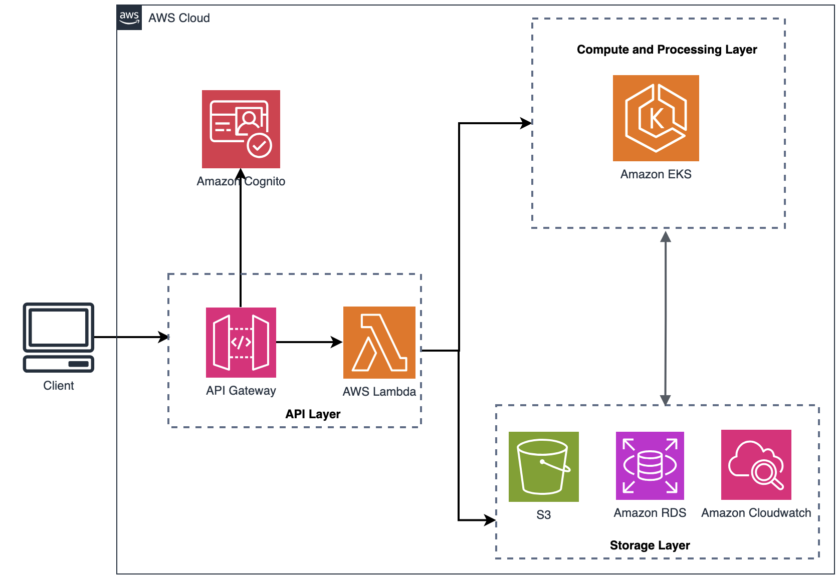
Figure 1: Architecture Diagram
LITHOLENS uses a unified API model to drive next-generation rock and mineral data analysis. This unified API created is a unified application programming interface that combines multiple services, data streams, and analytic capabilities into a single, powerful access point. Unlike traditional APIs—which might deliver basic, one-dimensional data—you can use the unified API to connect, analyze, and automate complex workflows across departments, vendors, and a wide variety of data sources all at once. With the unified REST API, users can submit geological analysis jobs, monitor progress, and retrieve results through a single interface. This API combines multiple services and data streams into one access point, so users can automate complex workflows across departments and data sources.
Architecture flow:
- Request Intake – Jobs are submitted through Amazon API Gateway with a payload specifying job parameters and EKS configuration.
- Job Orchestration – The API backend, running on AWS Lambda, provisions EKS containers with the appropriate configuration. User data scripts bootstrap each instance with required setup and execution commands.
- Execution and Data Flow
- Input data is retrieved from Amazon S3.
- Computation is performed on EKS pods using G6 instances.
- Logs and intermediate results are continuously tracked.
- Results are stored in S3 or persisted into RDS through dedicated API calls.
- Resource Management – Upon job completion, EKS containers instances automatically shut down, reducing costs.
Architecting for scale and efficiency
To handle variable workloads efficiently, ALS GeoAnalytics implemented a hybrid architecture that’s designed for both performance and cost. The system uses Amazon EKS for compute-intensive ML tasks while using AWS Lambda for lightweight API operations and job orchestration.
Key architectural decisions:
- Amazon EKS for ML Workloads – Deep learning model training and inference require sustained compute power with GPU acceleration. EKS provides the container orchestration needed to manage these workloads across G6 instances, with automatic scaling based on job queue depth.
- Lambda for API Gateway – Job submission, status checking, and result retrieval are handled through serverless functions. This removes the overhead of maintaining always-on API servers for sporadic client requests, reducing costs during low-usage periods.
- Pre-configured AMIs – Custom Amazon Machine Images contain all required dependencies and model artifacts, reducing container startup time from several minutes to under 30 seconds. This approach improves job throughput and reduces compute costs by minimizing idle time.
- Automated Resource Management -–EKS clusters scale down to zero when no jobs are queued, so compute resources are only consumed during active processing. Combined with S3 for data persistence and RDS for metadata, this creates a cost-effective architecture that scales with actual usage.
This design addresses the geological industry’s unpredictable workload patterns while maintaining the performance needed for complex computer vision tasks.
Business impact and results
LITHOLENS has seen success with 10 different mining companies on over 40 active projects, with substantially accelerated project completion and a standard analysis process used across all projects. This new approach has made mineral detection and classification more accurate while reducing the need for experts to visit sites. Teams can now trace how analysis decisions are made, grade minerals more consistently, and plan projects and assign resources more effectively. Real-time monitoring and reporting give managers up-to-the-minute information on how projects are progressing.
Conclusion
The massive scalability of Amazon EKS has allowed ALS GeoAnalytics to fundamentally transform how core logging and analysis is conducted. AWS suite of services enables LITHOLENS to efficiently implement computer vision and machine learning, bringing new operational capabilities to our customers and opening business opportunities throughout the mining industry. The success of LITHOLENS demonstrates how cloud computing and AI can help modernize a long-standing industry like mining, creating value through improved operational efficiency, accuracy, and scalability. ALS GeoAnalytics continues to evolve its platform on AWS, using cloud computing to push the boundaries of what’s possible, and looking to grow LITHOLENS in to promising applications in oil and gas, civil engineering, and even space exploration.
About the authors
How Synthesia optimizes generative AI video inference on Amazon EC2 G7e instances
Post Syndicated from Moises Hernandez original https://aws.amazon.com/blogs/architecture/how-synthesia-optimizes-generative-ai-video-inference-on-amazon-ec2-g7e-instances/
Synthesia, an enterprise-focused AI video platform, has transformed content creation, helping everyone to create video content without cameras or microphones. To achieve this, Synthesia allows its users to create video avatars that synthesize the likeness and voice of real people. Synthesia achieves this through a series of in-house developed models based on various architectures, including latent diffusion video generation models.
Customers like Synthesia often choose to host their models on Amazon Elastic Compute Cloud (Amazon EC2) instances because of the flexibility and control over the underlying hardware that the service provides, and among them they find the G7e instance family to be a cost-efficient option to serve GPU-memory intensive generative AI video models, giving customers access to NVIDIA RTX PRO 6000 Blackwell GPUs, with 96GB of GPU memory.
When generating videos using AI models with a Variational Auto Encoder (VAE) Decoder in the architecture, customers often find the GPU utilization is bottlenecked by the saving rate of the video frames to a file held on storage. This causes GPU stalls and reduces average GPU kernel utilization, which is the percentage of time the GPU is actively executing compute kernels rather than idle.
This post introduces a video decoding optimization technique that we have ideated in collaboration with Synthesia Research Engineering team, which we call Asynchronous Frame Generation Pipeline. Adopting this technique allows you to overlap GPU compute, device-to-host (D2H) data transfer, and host-side post-processing. In this post, we apply this technique to the VAE decoder of a Wan video generation model as an example, where our benchmarks on G7e show increased GPU kernel utilization from 82% to 99.9%, in turn leading to an 8.2% decrease in latency (and increase in throughput) for video decoding. We expect this technique to benefit any customer with a chunked video generation pipeline that transfers frames to host memory.
You can find an end-to-end example implementation of the Asynchronous Generation Pipeline applied to the Hugging Face Diffusers format of the Wan 2.2 14B Model in the associated GitHub repository.
In the following section, you will see how latent diffusion models generate video and why the traditional sequential decoding approach can lead to inefficient GPU utilization.
Understanding the sequential decoding bottleneck
Latent diffusion video generation models have emerged as powerful tools for generating temporally coherent video sequences. To reduce compute and memory requirements, these models perform the diffusion process in a compressed latent space of a variational auto-encoder (VAE), as depicted in the below figure, which has generally a much lower dimensionality than the originating video pixel space.
Fig. 1 High-level architecture of a VAE model. The depicted frames are taken from the Wan 2.2 repository sample video used in the example implementation in the next sections.
At inference time, a latent representation is initialized with noise and iteratively denoised via a Diffusion Process. To make sure that the output follows the text prompt, every denoising step is conditioned on the text input if present. After the final denoising step, the Diffusion Process yields a generated video that is still represented in the latent space of the VAE. The last step therefore consists in decoding the latent video back into a human-readable pixel video using the decoder part of the VAE.
Processing the whole latent or pixel video at once is usually too resource-intensive, even on large GPUs. It is therefore common to split the video along the temporal dimension and to decode video frames one latent frame at a time, resulting in a chunk of, for example, 4 consecutive pixel frames, as shown in Fig 2.
Fig.2 Decoding one latent results in a chunk of 4 time-consecutive pixel frames which are transferred from the GPU to the host.
Once a chunk has been decoded and processed on the GPU, the corresponding pixel frames must be transferred back to host (CPU) memory with a D2H transfer, so they can be written to a file or further processed. If you wait to transfer the video frames once the entire video has been decoded, the full decoded video must fit in GPU memory before being transferred, making this strategy hard to scale for arbitrarily long videos. A more memory-efficient alternative is to transfer the decoded frames every time a chunk is decoded, so that the GPU memory footprint of the decoder scales with the size of the chunk instead of the full video.
Traditionally, a newly generated set of frames in a chunk N is passed from GPU memory to CPU RAM synchronously, and it is committed to storage before the CPU can launch the CUDA kernels (referred to as kernels from now on) that process the N+1 chunk. This leads to systematic GPU stalls between chunks, as the copy from device to host prevents the GPU from immediately starting work on the next chunk, reducing overall hardware utilization, and in turn increasing processing time. We will refer to this synchronous process as Sequential Frame Generation Pipeline, which is depicted in Fig. 3.

Fig.3 Schematic representation of the Sequential Frame Generation Pipeline. Launching the kernels processing Chunk N+1 needs to wait for the full copy and storage of the frames in Chunk N.
In the following section, you will learn how to overcome this bottleneck using an asynchronous pipeline that overlaps GPU computation with data transfers and host-side processing.
Asynchronous Frame Generation Pipeline
To minimize GPU stalling, and in turn increase GPU utilization, you need to modify the Sequential Frame Generation Pipeline introduced in the previous section, so that all host-side CPU work (such as appending decoded frames to a file) runs in parallel with a stream of uninterrupted device-side kernels. This section shows you how to achieve this using as an example the implementation of an Asynchronous Wan VAE Decoder, which is implemented with PyTorch and you can find in the associated GitHub repository.
By default, PyTorch schedules work on a single (default) CUDA stream per device which executes the operations in issue order unless additional streams are explicitly created. To decouple compute and D2H copies, the implementation uses two CUDA streams so that the GPU is allowed to overlap compute kernels, which are enqueued on the default stream, and D2H copies on a dedicated copy stream. Compute kernels are enqueued on the default stream, which from now on can be referred to as Compute Stream, and D2H copies on a dedicated copy stream, namely the Copy Stream. In Fig. 4 you can find the full setup on a GPU accelerated instance (G7e in our example) depicted.
Fig. 4 High level diagram of the key components in our implementation of the Asynchronous Frame Generation Pipeline.
On the host side, kernel submissions are interleaved with D2H transfers and post-transfer processing and, to avoid host-side blocking calls and maximize GPU utilization the Asynchronous Frame Generation Pipeline introduces two mechanics:
- A dedicated Worker CPU thread responsible for reading chunks from Host Memory (RAM), and writing them to file, leaving the main Python thread to focus on launching kernels and scheduling D2H transfers.
- Two in-memory Buffers on the GPU Memory (VRAM), and on the Host Memory (RAM), and page-lock the required Host Memory buffers to make sure D2H copies are performed fully asynchronously.
Using a double-buffer strategy makes sure that for adjacent chunks the compute, D2H transfer, and host processing can overlap safely as they operate on distinct memory buffers.
Fig. 5 Schematic representation of the interplay between Events, Streams, Buffers, and Worker component in the Asynchronous Frame Generation Pipeline implementation. Events are depicted as left and right conditions, expressing what the process WAITs for, and ISSUEs when it has completed. The size of the boxes representing operations has been scaled to fit the text, and therefore not representative of the actual processing time.
Since buffers can be accessed concurrently by different components, the implementation introduces a synchronization mechanism to avoid different kernels and threads corrupting data held in the buffer. This can be achieved using CUDA Events which are used as a barrier that clears if it can answer closed questions such as: Has decoding of chunk N completed? You can find the interplay between Streams, Threads and Events depicted in Fig. 5.
G7e benchmark results
To quantify the impact of the Asynchronous Frame Generation pipeline, you can benchmark the decoding of a single 41 latent-frames test video for both the Synchronous and Asynchronous pipeline on a g7e.2xlarge EC2 instance using this sample notebook. To have a common baseline, the benchmarks are based on the unoptimized Hugging Face Diffusers Wan 2.2 14B model, and, in both cases, the benchmarking loop performs an initial full decoding cycle to let CUDA and PyTorch initialize and allocate memory pools and cache. After warmup, the benchmarking session carries out 10 consecutive full video decoding cycles. We have run an end-to-end run as an example and present the results in Table 1.
| Metric | Synchronous (time s /video) | Asynchronous (time s / video) |
| min | 21.98 | 20.16 |
| mean | 21.99 | 20.17 |
| P99 | 22.01 | 20.20 |
Table. 1 Benchmark results for 10 consecutive decoding runs for the Synchronous and Asynchronous pipelines.
The example results show a speed gain of up to 8.2% on this benchmark, decreasing the Real Time Factor of the decoder from 3.21 to 2.95. Considering the g7e.2xlarge pricing as of writing this post ($3.36 per GPU on-demand in the Ohio region), this leads to an average saving of $896 for decoding 1,000 hours of video on a single GPU. This is a theoretical saving, calculated assuming that the underlying model operates at full computational efficiency without bottlenecks.
To have a qualitative understanding of how this performance boost is achieved, you can profile both the Synchronous and Asynchronous pipelines using this sample notebook. The results for an example run are reported in Fig. 6 and Fig. 7, showing the absence of GPU stalls in the Asynchronous pipeline as opposed to the Synchronous pipeline.
Fig. 6 Profile of the Synchronous pipeline single thread and stream. As the main CPU thread is writing Chunk N frames to disk, the GPU stream stalls, waiting for the CPU to launch the kernels needed to process Chunk N+1
Fig.7 In the Asynchronous pipeline, the Compute Stream is not interrupted by the copying and writing of the frames to disk. The Main Thread is free to launch the processing kernels. This figure is displayed with a different zoom level than Fig. 6 to highlight the qualitative differences.
By focusing on the temporal axis for two consecutive chunks in the steady state, you can quantify the GPU kernel utilization increase, which, in our example run was 82% for the Synchronous case, increasing to 99.9% for the Asynchronous case.
Conclusion
In this post, we demonstrated how the Asynchronous Frame Generation Pipeline can improve GPU utilization when decoding latent videos on Amazon EC2 G7e instances. By decoupling GPU compute from device-to-host transfers and host-side I/O using dual CUDA streams, pinned memory buffers, and a dedicated worker thread, we eliminated the GPU stalls inherent in traditional synchronous decoding pipelines.
The sample benchmarks on the Wan 2.2 14B VAE decoder show an 8.2% reduction in decoding latency, translating to approximately $896 in savings per 1,000 hours of decoded video on a single GPU when considering the g7e.2xlarge pricing as of writing this post ($3.36 per GPU on-demand in the Ohio region). These gains come without any changes to model weights or inference quality, purely from better hardware utilization. We expect the kernel utilization gain to be even more impactful on optimized and compiled models, which make more efficient use of the GPU.
The techniques presented here are not specific to the Wan architecture, nor to the specific GPU utilized. Any chunked video generation pipeline that transfers frames to host memory can benefit from this approach. We encourage you to explore the associated sample implementation to experiment with how the Asynchronous Frame Generation Pipeline could be integrated into your own video generation workloads.
To get started with G7e instances for your generative AI video workloads, visit the Amazon EC2 G7e instance page.
About the authors
[$] In search of faster this_cpu operations
Post Syndicated from corbet original https://lwn.net/Articles/1073395/
The kernel’s this_cpu
operations are meant to speed access to per-CPU variables. They are
more optimal on some CPUs than others, though. During a
memory-management-track session at the 2026 Linux Storage,
Filesystem, Memory Management, and BPF Summit, Yang Shi proposed a
fundamental, and somewhat controversial, change to how these operations
work in order to provide better performance on a wider range of architectures.
[$] What’s brewing in CXL
Post Syndicated from corbet original https://lwn.net/Articles/1072858/
Compute
Express Link (CXL) is a technology intended to enable the provision of
“memory nodes” in data centers that provide (possibly shared) memory to
nearby CPUs. It has, Dan Williams said at the beginning of his
memory-management-track session on the topic at the 2026 Linux Storage,
Filesystem, Memory Management, and BPF Summit, “been making
“. He used the session to
memory-management problems worse since 2021
provide an overview of the ways in which CXL can be expected to extend that
record into the future.