Tag Archives: Industries

How Samsung achieved real-time pricing with AWS Lambda Response Streaming

2026-06-15 Vijay Naik

Post Syndicated from Vijay Naik original https://aws.amazon.com/blogs/architecture/how-samsung-achieved-real-time-pricing-with-aws-lambda-response-streaming/

This post is co-authored with Sathish Kumar and Christopher Chan from Samsung ecommerce.

In high-traffic ecommerce, achieving real-time pricing is critical to prevent price inconsistency. Pricing inconsistency creates cart shock and erodes trust. This isn’t broken software, it’s a symptom of architectural latency that you can address using AWS Lambda Response Streaming and Amazon CloudFront for systems aggregating data from multiple backend sources.

In this post, we walk through the legacy architecture challenges, the stateless streaming solution, key implementation patterns, and performance results—a pattern you can apply if you’re building high-traffic APIs that aggregate data from multiple backend sources.

Samsung.com is Samsung’s primary direct-to-consumer channel, selling smartphones, TVs, appliances, and accessories, each with multiple variants, offers, and regional pricing. This complexity makes real-time price accuracy especially important.

Samsung’s All Deals and Product Finder pages showcase these products during high-traffic events like Black Friday. To maintain low latency for these high-density Product Listing Pages (PLPs) and comparison tables, the legacy infrastructure relied on asynchronous caching, which introduced a desynchronization gap where the cached price drifted from the authoritative pricing engine.

Problem: Legacy middleware caching created a 1-hour desynchronization gap between the authoritative pricing engine and customer-facing pages.

Our approach: We dismantled the stateful Data Aggregation (DA) architecture and built a real-time Bulk Arbitration Engine (a stateless orchestration layer that queries the Pricing Engine directly at request time) using AWS Lambda Response Streaming and Amazon CloudFront edge caching.

Challenge: The Data Aggregation trap

When product listing pages need to display pricing for over 30 item combinations simultaneously, the latency of calling the Pricing Engine for each item combination individually becomes untenable. To solve this, we built a backend for frontend (BFF) service to do a “Data Aggregation. This DA service was designed to decouple the frontend from the heavy Pricing Engine.

It relied on a scheduled Cron Worker that ran hourly to fetch the entire product catalog. The worker would then precompute prices for every possible permutation of products and store them in a local cache.

While this improved read speeds, it created two significant failures:

1. The Permutation Explosion – The DA service had to precompute every combination just in case a customer viewed it.

The Math: 30 products × (Variants × Offers × Add-ons) = Thousands of records per page
Storage Impact: Cache grew exponentially with each new product variant added
Waste: Most precomputed combinations were never requested

2. The Synchronization Lag – Because the Cron job ran only once per hour, price changes (for example, flash sales) lagged significantly. Customers continued to see old prices until the next scheduled sync.

Business Impact: Flash sales showed incorrect old pricing until the next run time
Customer Trust: Cart shock when checkout price differed from product page price
Competitive Disadvantage: Competitors with real-time pricing gained market share

Legacy Data Aggregation architecture

Architecture diagram showing the legacy Data Aggregation layer between the Pricing Engine and CloudFront CDN.

Figure 1: Legacy Data Aggregation (DA) Architecture The legacy system relied on a scheduled Cron job, creating a distinct “Desynchronization Layer” between the Authority (Pricing) and the Customer. Precomputation of all product permutations consumed significant storage and compute resources.

The solution: Stateless streaming architecture

Intermediate layers storing data will eventually diverge from the source, so we collaborated with our AWS Technical Account Manager (TAM) and service teams to architect a new solution: the Bulk Arbitration Engine, a stateless orchestration layer that queries the Pricing Engine directly at request time.

The new architecture follows a Pass-Through pattern:

1. Client Request: The browser requests prices for 30 specific SKUs using a single HTTP GET request.

2. Streaming Orchestration: An AWS Lambda function fans out these 30 requests to the Pricing Engine in parallel.

3. Immediate Response: As the Pricing Engine returns data, the Lambda streams it immediately to the client without buffering.

Why Lambda Response Streaming?

We evaluated several alternatives before settling on this approach:

Traditional request-response pattern (buffered) – A standard Lambda invocation buffers the full response before returning it to the client, which negates the latency benefit of parallel fan-out. For 30 concurrent SKU lookups, this added seconds of wait time.
EC2 with improved caching – This was the legacy approach. Caching layers will eventually drift from the source of truth, which was the core problem we needed to solve.
Lambda Response Streaming – This was the only option that let us fan out requests in parallel, stream results as they arrived (reducing time-to-first-byte), and remain fully stateless with no intermediate cache to maintain or invalidate.

New stateless streaming architecture

New stateless Lambda Response Streaming architecture with CloudFront caching layer directly connected to Lambda function, which streams real-time responses from Pricing Engine without intermediate buffering. The diagram shows customer GET request to CloudFront, cache hit/miss routing decision, Lambda orchestration of parallel SKU lookups, and streaming response back through CloudFront edge.

Architecture diagram showing the stateless streaming solution with CloudFront connected directly to Lambda.

Figure 2: Stateless Streaming Architecture The new architecture eliminates the middleware cache. A high-performance stream connects the user directly to the pricing source of truth. CloudFront edge locations cache the response for 95% of traffic, while remaining requests go directly to Lambda for real-time pricing.

Implementation walkthrough

Transitioning to this new architecture required solving two specific technical constraints regarding CDN behavior and cold starts. We implemented the solution in three steps.

Step 1: Implementing the streaming handler

The core of our solution is the Node.js Lambda handler wrapped in awslambda.streamifyResponse(). This allows us to pipe data through a transformation and compression stream directly to the client as it becomes available.

We used a custom NDJSONTransform to convert pricing objects into newline-delimited JSON (NDJSON), allowing the browser to parse and render each price as it arrives rather than waiting for the complete response.

// Lambda Handler with Response Streaming
// File: lambda-handler.js

import * as awslambda from "aws-lambda";
import * as zlib from "zlib";
import { pipeline } from "stream/promises";
import { NDJSONTransform } from "./transforms/ndjson-transform.js";

// Constants
const PROCESSING_MODE = process.env.PROCESSING_MODE || "MODE_QUERYSTRING";
const MODE_QUERYSTRING = "MODE_QUERYSTRING";

// The Handler MUST be wrapped in streamifyResponse() to enable streaming
export const handler = awslambda.streamifyResponse(
  async (event, responseStream, _context) => {
    try {
      if (PROCESSING_MODE === MODE_QUERYSTRING) {
        // Set response metadata with status code and headers
        const httpResponseMetadata = {
          statusCode: 200,
          headers: {
            "Content-Type": "application/x-ndjson",
            "Content-Encoding": "gzip",
            "Cache-Control": "public, max-age=300", // 5 min cache
            "X-Custom-Header": "lambda-streaming",
          },
        };

        responseStream = awslambda.HttpResponseStream.from(
          responseStream,
          httpResponseMetadata
        );

        const ndjsonTransform = new NDJSONTransform();

        // Create gzip stream with fast compression level (Z_BEST_SPEED = Level 1)
        // Level 1 prioritizes speed over compression ratio for real-time responses
        const gzip = zlib.createGzip({
          level: zlib.constants.Z_BEST_SPEED,
        });

        // Process the request, writing to the gzip stream
        await processRequestUsingQueryString(event, ndjsonTransform, _context);

        // Pipeline: Transform → Compress → Send
        await pipeline(ndjsonTransform, gzip, responseStream);
      }

      // ... error handling
    } catch (error) {
      console.error("Lambda streaming error:", error);
      responseStream.destroy();
    } finally {
      await flushMetrics().catch(console.error);
    }
  }
);

Helper function to fan-out the requests in parallel:

// Process request: fan out SKU lookups in parallel
async function processRequestUsingQueryString(event, ndjsonTransform, context) {
  try {
    // Parse query string to extract SKU list
    const queryString = event.rawQueryString || "";
    const skus = parseCompressedQueryString(queryString);

    // Fetch pricing in parallel using Promise.all
    const pricingPromises = skus.map((sku) =>
      fetchPricingForSKU(sku).catch((err) => ({
        sku: sku.id,
        error: err.message,
      }))
    );

    const pricingResults = await Promise.all(pricingPromises);

    // Emit each result as a separate NDJSON line
    for (const result of pricingResults) {
      ndjsonTransform.write(result);
    }

    ndjsonTransform.end();
  } catch (error) {
    ndjsonTransform.destroy(error);
  }
}

The handler also uses helper functions for parsing the compressed query string (parseCompressedQueryString), fetching individual SKU prices with connection pooling (fetchPricingForSKU), and flushing metrics to Amazon CloudWatch (flushMetrics).

Key implementation details:

awslambda.streamifyResponse() wraps the handler so it streams data in real time instead of waiting for the full response from the pricing engine.
NDJSONTransform converts objects to newline-delimited JSON (one object per line)
GZIP (GNU zip) compression with Z_BEST_SPEED (Level 1) prioritizes speed over compression ratio
pipeline() handles error propagation and stream cleanup
Response headers include Cache-Control for CloudFront caching

Step 2: Compressing the request data into a GET request

We needed to send complex request data (30 SKUs, context metadata) to the API.

Constraint: CloudFront and standard HTTP specs treat POST requests as non-idempotent, meaning they are not cacheable by default.

Our approach: We developed a dense, compressed query string format to fit the complex request data into a standard GET request. Format: g=group1(p=SKU-A:1:p=SKU-B:2)…

This allowed us to strictly use GET requests, keeping the request URI within standard length limits (~800 bytes) while carrying the same data as a 3-4KB JSON body.

Client-Side Code: Building the Compressed Query String

// Client-side: Building the compressed query string format
// File: pricing-client.js

/**
 * Builds a compressed query string for bulk pricing requests
 * Format: g=group1(p=SKU-A:1:p=SKU-B:2:p=SKU-C:3)
 * @param {Array} skus - Array of SKU objects with { id, variant }
 * @param {Object} context - Customer context { customerId, region, sessionId }
 * @returns {string} Compressed query string
 */
function buildPricingQueryString(skus, context = {}) {
  if (!skus || skus.length === 0) {
    throw new Error("SKUs array cannot be empty");
  }

  if (skus.length > 30) {
    throw new Error("Maximum 30 SKUs per request. Split into multiple batches.");
  }

  // Build SKU portion: p=SKU-001:1:p=SKU-002:2
  const skuParts = skus
    .map((sku) => {
      const variant = sku.variant || 1;
      return `p=${sku.id}:${variant}`;
    })
    .join(":");

  // Build context portion (optional)
  let contextPart = "";
  if (context && Object.keys(context).length > 0) {
    const contextStr = Object.entries(context)
      .map(([key, value]) => `${key}=${value}`)
      .join(":");
    contextPart = `:c=${contextStr}`;
  }

  // Final format: g=group1(p=SKU-A:1:p=SKU-B:2:c=customerId=123:region=US-EAST-1)
  return `g=group1(${skuParts}${contextPart})`;
}

/**
 * Fetches pricing data with streaming NDJSON response parsing
 * Core pattern: read chunks, split by newlines, parse each line as JSON
 */
async function fetchPricingStream(skus, options = {}) {
  const queryString = buildPricingQueryString(skus);
  const url = `${options.baseUrl}?${queryString}`;
  const response = await fetch(url, {
    method: "GET",
    headers: { Accept: "application/x-ndjson" },
  });

  // Stream the response using the ReadableStream API
  const reader = response.body.getReader();
  const decoder = new TextDecoder();
  const pricingData = [];
  let buffer = "";

  while (true) {
    const { done, value } = await reader.read();
    if (done) break;

    // Decode chunk and append to buffer
    buffer += decoder.decode(value, { stream: true });

    // Split by newlines (NDJSON format: one JSON object per line)
    const lines = buffer.split("\n");

    // Keep the last incomplete line in buffer
    buffer = lines.pop() || "";

    // Parse each complete line as a JSON object
    for (const line of lines) {
      if (line.trim()) {
        const pricingObject = JSON.parse(line);
        pricingData.push(pricingObject);

        // Optional: update UI immediately as each price arrives
        if (options.onChunk) {
          options.onChunk(pricingObject);
        }
      }
    }
  }

  reader.releaseLock();
  return pricingData;
}

On page load, the client calls fetchPricingStream with up to 30 SKUs and an onChunk callback that updates each product’s DOM (Document Object Model) element as pricing chunks arrive. Helper functions handle updating individual price elements, displaying variant information, and gracefully degrading with a user-friendly message if pricing is temporarily unavailable.

Step 3: Configuring CloudFront for uncacheable requests

To allow CloudFront to cache these complex GET requests effectively, we configured a precise Cache Policy that includes all query strings and specific headers.

# Terraform: CloudFront Cache Policy Configuration
# File: cloudfront-cache-policy.tf

resource "aws_cloudfront_cache_policy" "pricing-cache-policy" {
  name = "${var.lambda_function_name}-cache-policy"

  # TTL Configuration
  default_ttl = 300  # 5 minutes
  max_ttl     = 1800 # 30 minutes
  min_ttl     = 300   # 5 minute

  parameters_in_cache_key_and_forwarded_to_origin {
    # Don't cache based on cookies (we don't use them)
    cookies_config {
      cookie_behavior = "none"
    }

    # Allowlist specific headers for cache key
    headers_config {
      header_behavior = "whitelist"
      headers {
        items = [
          "x-ecom-pricing-1",   # Custom headers (anonymized)
          "x-ecom-pricing-2",  
          "x-ecom-pricing-3"    
        ]
      }
    }

    # Include query strings in cache key
    # This verifies different SKU combinations have separate cache entries
    query_strings_config {
      query_string_behavior = "all"
    }

    # Enable automatic GZIP compression
    enable_accept_encoding_gzip = true
  }
}

# CloudFront Origin Request Policy (forward headers to Lambda)
resource "aws_cloudfront_origin_request_policy" "pricing-origin-policy" {
  name = "${var.lambda_function_name}-origin-policy"

  headers_config {
    header_behavior = "whitelist"
    headers {
      items = [
        "x-ecom-pricing-1",
        "x-ecom-pricing-2",
        "x-ecom-pricing-3"
      ]
    }
  }

  query_strings_config {
    query_string_behavior = "all"
  }

  cookies_config {
    cookie_behavior = "none"
  }
}

The CloudFront distribution itself is configured with HTTPS-only viewer protocol, the cache policy and origin request policy as shown in the preceding section, and points to the Lambda as its origin through HTTPS.

Cache policy highlights:

5-minute default TTL balances freshness and cache efficiency
Query strings included in cache key (different SKU combos = separate cache entries)
Header allowlisting allows custom pricing variants
Automatic GZIP compression reduces bandwidth
5–30 minute TTL range provides flexibility for different content

Performance optimization results

We optimized the system through four distinct phases, testing each configuration with K6 load test scripts (500 concurrent users, 30 items per request) to simulate high-traffic events like Black Friday.

Phase 1: The baseline (Global VPN)

We tested our initial proof-of-concept with the default network configuration, where all outbound traffic (including requests to AWS services like Lambda) was routed through a global VPN, forcing traffic onto the public network and back into the AWS backbone, adding unnecessary network hops and delays. The Lambda used a standard buffered response with no compression. The results were suboptimal (4,500ms P90) because connection overhead dominated the request.

DNS resolution: approximately 50 ms
TCP handshake: approximately 100 ms
TLS negotiation: approximately 150 ms
Total connection overhead: approximately 300 ms per call

This overhead created a massive bottleneck for latency before business logic even ran.

Phase 2: Amazon VPC Peering and warm starts

To remove the network penalty, we acted on two fronts:

First: Moved the Lambda inside an Amazon Virtual Private Cloud (Amazon VPC) peered directly to the pricing origin, cutting DNS and TLS overhead to near zero for internal calls.
Second: Enabled Provisioned Concurrency for Lambda to remove the 500–1000 ms cold start latency.

With these changes, P90 latency dropped to 1,000 ms, a 4.5x improvement, but still not real-time enough.

Phase 3: HTTP/2 and GZIP compression

The remaining bottleneck was the sheer size of the data transfer. We targeted two optimizations:

HTTP/2 Multiplexing: Enabled HTTP/2 multiplexing to reuse a single TCP connection for the 30 parallel SKU lookups, saving seconds of cumulative handshake time.
GZIP Compression: Applied GZIP compression (Level 1 / Z_BEST_SPEED), which reduced the response size by 76 percent (170KB → 40KB).

These two optimizations brought P90 latency down to 218 ms.

Phase 4: Production (edge caching)

In the final phase, we layered CloudFront edge caching on top of the optimized Lambda. Because we had successfully converted our request data to a GET request (Step 2), we could now cache the computed prices for 95 percent of incoming traffic.The final P90 latency landed at 50 ms.In practice, the 95 percent cache hit ratio means only 1 in 20 requests actually invokes the Lambda function; the rest are served directly from CloudFront edge locations closest to the customer. During peak events like Black Friday, this translates to millions of requests served at edge speed without touching the origin, keeping both latency and compute costs minimal.

Performance metrics table

Metric	Phase 1 (Baseline)	Phase 2 (VPC)	Phase 3 (HTTP/2)	Phase 4 (Production)
P50 Latency	1,670 ms	501 ms	176 ms	35 ms
P90 Latency	4,500 ms	1,000 ms	218 ms	50 ms
P99 Latency	5,100 ms	2,400 ms	500 ms	150 ms
Cache Hit Ratio	<1%	<1%	<1%	95%
Response Size	170 KB	170 KB	40 KB	40 KB
Concurrent Users	500	500	500	500
P90 Improvement vs Baseline	1x	4.5x	20x	90x

The following chart shows P90 latency improvements across each optimization phase.

Latency improvements across four optimization phases.

K6 load test configuration:

// A sample K6 load test script
import http from 'k6/http';
import { check } from 'k6';

export let options = {
  stages: [
    { duration: '2m', target: 100 },  // Ramp up
    { duration: '5m', target: 500 },  // Stay at 500 concurrent users
    { duration: '2m', target: 0 },    // Ramp down
  ],
  thresholds: {
    http_req_duration: ['p(90)<100', 'p(99)<500'], // P90 < 100ms, P99 < 500ms
  },
};

export default function () {
  const url = 'https://api.example.com/pricing?g=group1(p=SKU-001:1:p=SKU-002:2:...)';
  const res = http.get(url);
  
  check(res, {
    'status is 200': (r) => r.status === 200,
    'response has content': (r) => r.body.length > 0,
  });
}

Resilience, scale, and security considerations

Beyond latency, we designed the system to handle failure gracefully, scale under load, and protect data in transit.

Batching limits

The 30-item limit per request is intentional. If a page requires more (for example, 50 items), the client logic splits them into multiple parallel batches.–We chose 30 because of the following:

Lambda execution time under 5 seconds
Prevents timeout issues during high latency
Balances parallel requests vs. Lambda concurrency limits
Typical product listing pages show 20–30 items

async function fetchLargePricingBatch(skus) {
  const BATCH_SIZE = 30;
  const batches = [];

  // Split into 30-item chunks
  for (let i = 0; i < skus.length; i += BATCH_SIZE) {
    batches.push(skus.slice(i, i + BATCH_SIZE));
  }

  // Fetch all batches in parallel
  const results = await Promise.all(
    batches.map((batch) =>
      fetchPricingStream(batch, { timeout: 30000 })
    )
  );

  // Flatten results
  return results.flat();
}

Partial failures

The streaming architecture is resilient. If pricing for one item fails, the stream doesn’t crash; it continues processing the remaining items, so the user still sees a mostly complete page.

Partial failure handling:

async function processRequestUsingQueryString(event, ndjsonTransform, context) {
  const skus = parseCompressedQueryString(event.rawQueryString);

  for (const sku of skus) {
    try {
      const pricing = await fetchPricingForSKU(sku);
      ndjsonTransform.write(pricing);
    } catch (error) {
      // Emit error object but continue processing other SKUs
      ndjsonTransform.write({
        sku: sku.id,
        variant: sku.variant,
        error: error.message,
        timestamp: new Date().toISOString(),
      });
    }
  }

  ndjsonTransform.end();
}

Data protection

While constructing the query string on the client exposes the request structure, this data (SKUs, variants) is already public. The actual pricing logic and business rules remain securely protected within the Pricing Engine.
Data in transit encrypted with TLS 1.3.
Amazon VPC endpoint connection to pricing engine (no internet exposure).
No sensitive data logged (PII, pricing algorithms excluded).
CloudTrail logs API calls for audit trail.

Conclusion

Stale pricing forces engineering teams to choose between freshness and scale. With the Data Aggregation pattern, we attempted to maintain both but compromised on data integrity due to the lag inherent in scheduled synchronization.By using AWS Lambda Response Streaming and Amazon CloudFront, we removed the need for a synchronization layer entirely. The result is a system that delivers the 50 ms latency required for a smooth user experience while supporting price consistency between the product page and checkout.

Beyond performance, this architecture significantly reduced operational footprint: compute fleet shrank from over 100 auto-scaled instances during peak events to only 5–10 Lambda functions, lowering maintenance and operational costs. This outcome was the result of close collaboration between Samsung’s ecommerce engineering team, our AWS Technical Account Manager (TAM), and the Lambda and CloudFront service teams, who helped architect the solution, review design decisions, and guide Samsung through production readiness. This technique applies to similar high-traffic data aggregation scenarios: product catalogs, inventory systems, recommendation engines, or services that combine multiple backend responses in real-time.

To get started, identify your highest-latency aggregation endpoints, evaluate whether your request data can be converted to cacheable GET requests and implement Lambda Response Streaming for a single endpoint before migrating your full API

Resources: – AWS Lambda Response Streaming documentation – Lambda Response Streaming tutorial – Amazon CloudFront Developer Guide – CloudFront cache policies

Learn more

For more on the concepts and technologies discussed in this post:

Introducing AWS Lambda Response Streaming – The AWS Compute blog post that introduces the streaming pattern used in this solution
Tutorial: Creating a Response Streaming Lambda Function – Step-by-step tutorial to build your first streaming Lambda function
CloudFront Best Practices – Best practices for configuring CloudFront distributions
NDJSON Format – The newline-delimited JSON specification used for incremental response parsing
Node.js Streams API – The Node.js streams documentation underpinning the Transform and Pipeline patterns
Terraform AWS Provider – Infrastructure as code provider used for the CloudFront and WAF configurations
AWS Prescriptive Guidance: Load Testing – AWS guidance on load testing tools including K6

About the authors

How Zynga scaled multi-warehouse data governance with Amazon Redshift federated permissions

2026-05-27 Johan Eklund, Matthew Wongkee, Noelia Tardón

Post Syndicated from Johan Eklund, Matthew Wongkee, Noelia Tardón original https://aws.amazon.com/blogs/big-data/how-zynga-scaled-multi-warehouse-data-governance-with-amazon-redshift-federated-permissions/

Zynga, a global leader in interactive entertainment operates a portfolio of mobile game studios including Socialpoint, the creators of Dragon City and Monster Legends. Zynga’s analytics platform processes telemetry and revenue data across studios using Amazon Redshift as its central data warehouse.

As Zynga expanded its analytics architecture to include individual studios with their own compute environments, the team faced a challenge: how to maintain centralized data governance while granting studios independent query capacity. Their existing approach to permission management introduced lag and required custom infrastructure if scaled to multiple warehouses.

In this post, we walk through how Zynga adopted Amazon Redshift federated permissions and AWS IAM Identity Center to enforce consistent, tiered data access across provisioned and serverless Amazon Redshift environments without building custom synchronization pipelines.

The challenge

Zynga needed to onboard Socialpoint’s current Amazon Redshift workloads and make Zynga’s central data available to them. Zynga’s existing production cluster would house the Socialpoint raw data, but the compute would come from another warehouse set up as a consumer. At the same time, Zynga’s data access control policies would need to be enforced across all warehouses. Zynga uses a tiered access control policy which would need to be synced across all consumers with no permission lag or manual grant synchronization.

During the migration, Socialpoint’s specific extract, transform, and load (ETL) processes would be included in Zynga’s central ETLs and their data ingestion pipeline would be replaced by Zynga’s latest generation of data ingestion infrastructure. Because the migration process happens in stages, Amazon Redshift sizing would also gradually need to increase.

The team evaluated two alternatives before arriving at a solution:

AWS Lake Formation couldn’t manage local and cross-cluster permissions using the same interface, and required AWS Access and Identity Management (IAM) or IAM Identity Center authentication for all users including service accounts.
Manual grants on consumer clusters introduced a delay between when permissions were updated on the producer and when they took effect on the consumer. This approach would also require an external job that synced permissions and would be unlikely to scale well beyond 2–3 consumers.

Solution overview

Zynga implemented a solution using three AWS services working together:

Amazon Redshift federated permissions enabled cross-cluster queries without explicit data shares. Permissions granted on the producer cluster propagate immediately to consumer workgroups through AWS Glue Data Catalog registration.
AWS IAM Identity Center provides unified authentication through federation with Okta. When users sign in, their Okta group memberships are provisioned through a System for Cross-domain Identity Management (SCIM) and automatically map to Amazon Redshift roles, removing the need for external synchronization jobs.
Amazon Redshift Serverless provides the compute layer for Socialpoint, scaling to zero when idle and avoiding the need to pre-size a provisioned cluster during the migration period.

The architecture uses a dual-grant approach where every permission is granted to both an IAM Identity Center group (for users) and a federated IAM role (for service accounts). This gives both authentication paths the same access.

How it works

Authentication with IAM Identity Center

Zynga’s existing Okta directory syncs to IAM Identity Center, which is connected to the Amazon Redshift Serverless workgroup. When a user authenticates, Amazon Redshift automatically creates a user mapped to their email address and assigns them to roles based on their Okta group membership.

For example, an analyst in the Gamma Tier group signs in and is automatically assigned the AWSIDC:role.sso.gamma role in Amazon Redshift. No manual role assignment or synchronization job is required.

Service accounts, used for programmatic access, authenticate differently. Either using their IAM role and calling the get-credentials API, or by using the new federated permissions feature. Each service account assumes a federated IAM role, which creates a corresponding federated user in Amazon Redshift (for example, IAMR:role_iam_gamma).

Figure 1 – Identity layer

The dual-grant approach

To ensure that both users and service accounts can access the same data, every read permission is granted to both the IAM Identity Center group and the federated IAM role in a single statement:

GRANT SELECT ON schema.table TO
	'IAMR:role_iam_gamma',
	ROLE 'AWSIDC:role.sso.gamma';

Transitioning the producer cluster

The shared provisioned cluster already had active users with local grants. To avoid disruption, Zynga implemented a tri-grant approach on the producer during the transition period. Existing stored procedures were modified to grant permissions to three targets: the legacy local role, the IAM Identity Center group, and the federated IAM role.

GRANT SELECT ON schema.table TO
	ROLE role_rs_gamma,
	ROLE 'AWSIDC:role.sso.gamma','IAMR:role_iam_gamma';

This approach maintains backward compatibility for existing users on the producer while enabling immediate access from the new serverless workgroup. The long-term plan includes migration of all producer users to IAM Identity Center and retire the legacy local grants.

Stored procedures for consistent governance

Rather than requiring users to construct dual-grant statements manually, Zynga created stored procedures that encapsulate the grant logic:

grant_read accepts a table name and access tier, then issues the appropriate dual-grant for both the IAM Identity Center group and the federated IAM role.
grant_write grants data definition language (DDL) and data manipulation language (DML) permissions to the appropriate team-based role.

This provides a consistent interface for permission management regardless of which cluster or workgroup that the user is on.

Figure 2 – Data and compute layer

Results

The migration delivered measurable improvements:

Immediate permission propagation – Grants on the producer cluster took effect on the consumer workgroup instantly, replacing a process that previously required manual intervention and introduced lag.
Zero additional infrastructure cost – Federated permissions, federated queries, and IAM Identity Center added no incremental costs to the architecture.
Removed custom synchronization – The team removed the need for Lake Formation configurations, external AWS Lambda functions, and Airflow workflows for permission management.
Scalable pattern – The same architecture can be extended to additional studio workgroups without duplicating permission management logic.

Lessons learned

Zynga adopted federated permissions shortly after the feature launched in US West Oregon (us-west-2) in January 2026. The team shared several observations from their early adoption:

Run a proof of concept first. The team validated the full permission model in a test environment before deploying to production, including testing that existing data shares to other clusters were not disrupted.
Plan for the dual-grant requirement. Because IAM Identity Center users and federated IAM roles are distinct identity types, every read permission requires two grants. Encapsulating this in stored procedures prevents errors and reduces cognitive overhead.
Start with serverless for new workloads. With Amazon Redshift Serverless, the team can avoid sizing decisions during the migration period. If usage patterns later justify it, they can migrate to a provisioned cluster from a serverless snapshot with minimal downtime.
Engage with AWS. As an early adopter of a new feature, Zynga maintained regular contact with the Amazon Redshift team through their AWS Technical Account Manager to report issues and request enhancements.

Conclusion

Zynga’s adoption of Amazon Redshift federated permissions demonstrates how organizations with multi-cluster Amazon Redshift architectures can enforce centralized data governance without building custom synchronization infrastructure. By combining federated permissions with IAM Identity Center and Amazon Redshift Serverless, the team established a pattern that scales to additional studios while maintaining consistent access controls and reducing operational overhead.

To learn more about the services used in this post, see the following resources:

About the authors

How ALS GeoAnalytics LITHOLENS ™ revolutionizes core logging through machine learning with Amazon EKS

2026-05-19 Saransh Burman

Post Syndicated from Saransh Burman original https://aws.amazon.com/blogs/architecture/how-als-geoanalytics-litholens-revolutionizes-core-logging-through-machine-learning-with-amazon-eks/

In the mining industry, accurate geological analysis is required for improving mine design and development. Traditionally, this involved labor-intensive and time-consuming on-site inspections of drill core samples, often conducted in remote and challenging environments. ALS GeoAnalytics has streamlined this process through its LITHOLENS platform, a machine learning (ML)-powered system that uses deep learning and machine vision to automate core logging. LITHOLENS significantly enhances data consistency, operational efficiency, and scalability while significantly reducing logging-related costs and lowering greenhouse gas emissions to support sustainable mineral extraction.

This post explores how ALS GeoAnalytics successfully deployed LITHOLENS with Amazon Elastic Kubernetes Service (Amazon EKS) to scale model training and inference while minimizing cost.

The challenge

Development of a new mine involves the creation of a 3D map of the ore body, known as a geological or resource model. This model drives all future design decisions and creating it requires drilling thousands of holes throughout the ore body to examine the structure and composition of the samples extracted. This process is subject to numerous challenges that affect both active and historical drilling campaigns. Challenges such as:

Remote site access requiring geologists to travel long distances to visually inspect physical core boxes
Subjective interpretations led to inconsistencies, with different experts often producing varying geological logs
Underutilized historical imagery from past campaigns lacked standardized tools for meaningful analysis
Lost or degraded physical samples made it difficult to revisit legacy data or validate past interpretations
Limited transparency in logging and decision-making processes hindered collaboration and accountability
Scheduling bottlenecks arose from reliance on a small pool of qualified experts
Non-standardized data collection methods prevented effective scaling and cross-project comparison

These limitations not only delayed project timelines but also restricted the ability to generate reliable, high-resolution geological insights—ultimately impeding the speed and effectiveness of exploration strategies.

Machine learning at geological scale

ALS GeoAnalytics developed a comprehensive suite of machine learning and computer vision models to automate geological and geotechnical logging, transforming raw core imagery and data into actionable insights.

A machine learning pipeline formed the foundation for high-resolution visual analysis. It begins with the Color Extraction module, which scans each image to identify unique pixel colors and store the results in Amazon Simple Storage Service (Amazon S3). This data is fed into the Color Clustering module, where users can specify clustering parameters and choose from algorithms such as K-Means, which assigns pixels to clusters based on proximity to centroids, or the Gaussian Mixture Model (GMM), which uses probabilistic distributions to capture more complex variance structures within the color data. These methods effectively reduced image complexity and helped highlight mineralogical variation.

To quantify color composition along the core, the Percentage Report module was introduced. It segmented each image into user-defined sections (for example, 20 cm intervals) and calculated the proportional distribution of each color cluster, enabling spatial analysis of lithological patterns.

On the deep learning front, the team developed and deployed an advanced suite of models tailored for geological and geotechnical analysis. A highlight of this work was the development of RoQE Net, a state-of-the-art neural network designed for geotechnical parameter extraction. RoQE Net demonstrated exceptional accuracy in computing Rock Quality Designation (RQD) and extracting alpha angles, key metrics for assessing core integrity and rock mass quality. In parallel, VeinNet and CobbleNet were engineered to identify and map complex geological features such as veins, cobbles, and lithological structures with high precision. These models were benchmarked against industry standards and consistently outperformed traditional methods in terms of accuracy, reliability, and scalability.Together, these machine learning and deep learning components form the backbone of the LITHOLENS platform—delivering automated, scalable, and highly accurate geological intelligence that accelerates decision-making and enhances the efficiency of exploration and resource modeling workflows.

Solution architecture

ALS GeoAnalytics built LITHOLENS on AWS using a hybrid architecture that combines containerized workloads with serverless components. The system uses Amazon EKS for compute-intensive machine learning tasks, AWS Lambda for API operations, Amazon S3 for data storage, and Amazon Relational Database Service (Amazon RDS) for structured data management.

Figure 1: Architecture Diagram

LITHOLENS uses a unified API model to drive next-generation rock and mineral data analysis. This unified API created is a unified application programming interface that combines multiple services, data streams, and analytic capabilities into a single, powerful access point. Unlike traditional APIs—which might deliver basic, one-dimensional data—you can use the unified API to connect, analyze, and automate complex workflows across departments, vendors, and a wide variety of data sources all at once. With the unified REST API, users can submit geological analysis jobs, monitor progress, and retrieve results through a single interface. This API combines multiple services and data streams into one access point, so users can automate complex workflows across departments and data sources.

Architecture flow:

Request Intake – Jobs are submitted through Amazon API Gateway with a payload specifying job parameters and EKS configuration.
Job Orchestration – The API backend, running on AWS Lambda, provisions EKS containers with the appropriate configuration. User data scripts bootstrap each instance with required setup and execution commands.
Execution and Data Flow
- Input data is retrieved from Amazon S3.
- Computation is performed on EKS pods using G6 instances.
- Logs and intermediate results are continuously tracked.
- Results are stored in S3 or persisted into RDS through dedicated API calls.
Resource Management – Upon job completion, EKS containers instances automatically shut down, reducing costs.

Architecting for scale and efficiency

To handle variable workloads efficiently, ALS GeoAnalytics implemented a hybrid architecture that’s designed for both performance and cost. The system uses Amazon EKS for compute-intensive ML tasks while using AWS Lambda for lightweight API operations and job orchestration.

Key architectural decisions:

Amazon EKS for ML Workloads – Deep learning model training and inference require sustained compute power with GPU acceleration. EKS provides the container orchestration needed to manage these workloads across G6 instances, with automatic scaling based on job queue depth.
Lambda for API Gateway – Job submission, status checking, and result retrieval are handled through serverless functions. This removes the overhead of maintaining always-on API servers for sporadic client requests, reducing costs during low-usage periods.
Pre-configured AMIs – Custom Amazon Machine Images contain all required dependencies and model artifacts, reducing container startup time from several minutes to under 30 seconds. This approach improves job throughput and reduces compute costs by minimizing idle time.
Automated Resource Management -–EKS clusters scale down to zero when no jobs are queued, so compute resources are only consumed during active processing. Combined with S3 for data persistence and RDS for metadata, this creates a cost-effective architecture that scales with actual usage.

This design addresses the geological industry’s unpredictable workload patterns while maintaining the performance needed for complex computer vision tasks.

Business impact and results

LITHOLENS has seen success with 10 different mining companies on over 40 active projects, with substantially accelerated project completion and a standard analysis process used across all projects. This new approach has made mineral detection and classification more accurate while reducing the need for experts to visit sites. Teams can now trace how analysis decisions are made, grade minerals more consistently, and plan projects and assign resources more effectively. Real-time monitoring and reporting give managers up-to-the-minute information on how projects are progressing.

Conclusion

The massive scalability of Amazon EKS has allowed ALS GeoAnalytics to fundamentally transform how core logging and analysis is conducted. AWS suite of services enables LITHOLENS to efficiently implement computer vision and machine learning, bringing new operational capabilities to our customers and opening business opportunities throughout the mining industry. The success of LITHOLENS demonstrates how cloud computing and AI can help modernize a long-standing industry like mining, creating value through improved operational efficiency, accuracy, and scalability. ALS GeoAnalytics continues to evolve its platform on AWS, using cloud computing to push the boundaries of what’s possible, and looking to grow LITHOLENS in to promising applications in oil and gas, civil engineering, and even space exploration.

About the authors

Building hybrid multi-tenant architecture for stateful services on AWS

2026-05-12 Vasu Raj

Post Syndicated from Vasu Raj original https://aws.amazon.com/blogs/architecture/building-hybrid-multi-tenant-architecture-for-stateful-services-on-aws/

Running a large-scale ad-serving infrastructure presents unique challenges when balancing tenant isolation with operational efficiency. Our infrastructure handles millions of requests per second and generates billions of dollars in annual advertising revenue, serving ads across multiple properties and systems.

The cellular architecture problem

Earlier, we had a cellular architecture where we allocated each AWS account with Application Load Balancer (ALB) and Amazon Elastic Container Service (Amazon ECS) to a given tenant. This approach provided accurate isolation but created the following significant operational challenges.

The scale problem: Supporting only 18 clients across four AWS Regions requires 181 separate targets. Our team configured dedicated AWS accounts, VPCs, load balancers, AWS Identity and Access Management (IAM) roles, and downstream service connections for each client.
The efficiency problem: Our servers spent more than 98 percent of their time waiting and less than 1 percent executing code. Average CPU utilization sat at 3 percent, and memory at 19 percent. We were paying for massive infrastructure that remained idle most of the time.
The onboarding problem: Bringing a new client online took approximately 52 days—roughly two weeks for AWS account provisioning, three weeks for VPC and networking setup, one week for IAM role configuration, and two weeks for downstream service integration and testing.
The scalability problem: When traffic grows or a new client joined, our only option is to spin up an entirely new cell and migrate to the client. We couldn’t support concurrent tier-1 live events—multiple high-value games couldn’t run simultaneously, forcing us to divert traffic to alternative systems.
The noisy neighbor problem: Despite our isolation efforts, we still experienced performance degradation when tenants shared infrastructure, affecting service quality and reliability.

Why we needed dedicated compute

Our ad-serving platform is a stateful service that loads and maintains data in memory for each tenant rather than fetching it from a database on every request. This in-memory state improves performance but creates the noisy neighbor problem when tenants share infrastructure.When two tenants share a cluster, their in-memory data competes for the same heap. A tenant with a large dataset can trigger out-of-memory conditions that affect its neighbors. This made shared-task and shared-cluster approaches challenging our stateful workloads.We needed a solution that maintained cluster-level isolation while dramatically improving operational efficiency.

Solution overview

We designed a hybrid multi-tenant architecture that provides cluster-level isolation within shared accounts. Here’s what we implemented:

Pre-integration model: Instead of provisioning VPCs, IAM roles, and downstream service connections for each new tenant, we created a configuration-driven infrastructure where these integrations are established once and reused across tenants.
Amazon Route 53 weighted routing: We implemented Route 53 weighted routing to enable gradual traffic migration between clusters without client-side changes. This allowed us to shift tenants between tiers as their traffic patterns evolved.
AWS PrivateLink connectivity: We established AWS PrivateLink endpoints that all tenants share, removing the need for us to set up new VPC peering or Transit Gateway connections for each tenant and reducing network configuration overhead by 80 percent.
Tier-based architecture: We organized our infrastructure into tiers (High TPS, Standard TPS, Low TPS) with multiple cells per tier, enabling horizontal scaling without the operational burden of per-tenant AWS accounts.
Configuration-driven onboarding: New tenant onboarding became a configuration change rather than an infrastructure provisioning exercise, dramatically reducing time and manual effort.

The architecture is organized around three nested levels of hierarchy. A tier is the top-level grouping—a logical classification of tenants that share a common infrastructure footprint. A tier spans one or more cells, where each cell is an AWS account boundary that represents the unit of horizontal scale-out at the account level. Within each cell, one or more infra groups serve as the self-contained infrastructure unit: a VPC, an Application Load Balancer, a set of ECS clusters (one per tenant), IAM roles, and a monitoring stack.

Why three levels? As you scale from 10 to 100 to 1,000 tenants, you will reach different AWS limits at different scales. Application Load Balancer target group limits constrain how many tenants fit in a single load balancer. AWS account limits on Elastic Network Interfaces (ENIs) and VPC endpoints constrain how many load balancers fit in a single account. This three-level hierarchy gives you two independent scaling levers to address each constraint—add infra groups to scale within an account and add cells to scale across accounts. The key design principle is that we pre-wire downstream service dependencies at tier creation, not at tenant onboarding. AWS PrivateLink connections from the tier VPC to each downstream service VPC are established after the tier is provisioned. After onboarding tenants to that tier, they automatically inherit full downstream connectivity. This single architectural decision is the primary reason for the 80 percent reduction in infrastructure setup steps. Route 53 performs weighted DNS routing across Application Load Balancers in multiple infra groups and cell accounts, enabling horizontal scale-out without client-side changes.

The following diagram illustrates the full architecture: Route 53 distributes traffic across ALBs in multiple infra groups within a single cell account, each ALB routes to tenant-specific ECS clusters using listener rules and target groups, and the clusters share tier-level PrivateLink connections to downstream services.

Multi-Tenant Architecture Diagram

Figure 1: Hybrid multi-tenant architecture showing Route 53 weighted routing, Application Load Balancer listener rules, dedicated ECS clusters per tenant, and shared AWS PrivateLink connections to downstream services.

Prerequisites

Before you build this architecture, make sure that you have the following:An AWS account configured with least privileged permissions to create VPCs, Application Load Balancers, ECS clusters, Route 53 hosted zones, and VPC endpoints. You also need the AWS Command Line Interface (AWS CLI) version 2.x or later installed and configured with appropriate credentials. This walkthrough assumes intermediate familiarity with Amazon ECS, Application Load Balancer, and Amazon Route 53—specifically ECS task definitions, Application Load Balancer listener rules, and Route 53 routing policies. You also need at least one downstream service exposing a VPC endpoint service for AWS PrivateLink connectivity.

Estimated time to complete: 2–3 hours.

Walkthrough

This walkthrough shows you how to build the previously described hybrid multi-tenant architecture. You will configure Route 53 weighted routing, deploy an ALB with tenant-specific listener rules, create dedicated ECS clusters per tenant, and establish AWS PrivateLink connectivity to shared downstream services. These will be done in a way that makes future tenant onboarding a configuration-only operation.

Step 1: Configure Route 53 Regional endpoints with weighted routing

Each tier exposes a single Regional DNS endpoint (for example, tier-1.us-east-1.example.com) backed by Route 53 weighted routing records. You can configure Route 53 to use weighted routing to help distribute traffic across ALBs in multiple AWS accounts. When you add a new account to the tier for horizontal scale-out, add a new weighted record. You don’t need to change existing tenant DNS entries.

To configure Route 53 weighted routing for a tier:

Open the Amazon Route 53 console and choose Hosted zones.
Select or create the hosted zone for your tier.
Choose Create record and select Weighted as the routing policy.
Set the record name to your tier endpoint (for example, tier-1.us-east-1.example.com), record type to A, and configure an alias pointing to the ALB in your first AWS account.
Set the Weight to 50 and provide a unique Set ID (for example, account-1).
Enable Evaluate target health so Route 53 helps make sure that it directs traffic to healthy ALBs when you configure health evaluation.
Repeat for each additional AWS account in the tier, using matching weights.

Alternatively, run the following AWS CLI command to create the first weighted record:

aws route53 change-resource-record-sets \
  --hosted-zone-id YOUR_HOSTED_ZONE_ID \
  --change-batch '{
    "Changes": [{
      "Action": "CREATE",
      "ResourceRecordSet": {
        "Name": "tier-1.us-east-1.example.com",
        "Type": "A",
        "SetIdentifier": "account-1",
        "Weight": 50,
        "AliasTarget": {
          "HostedZoneId": "Z35S*****K",
          "DNSName": "your-alb.us-east-1.elb.amazonaws.com",
          "EvaluateTargetHealth": true
        }
      }
    }]
  }'

Note: Replace Z35S****K with the hosted zone ID for your ALB’s AWS Region. For more information, see Elastic Load Balancing endpoints and quotas.

Route 53 supports up to 10,000 weighted records per hosted zone, so this approach scales to thousands of AWS accounts without architectural changes. For more information about weighted routing, see Weighted routing in the Amazon Route 53 Developer Guide.

Step 2: Deploy an Application Load Balancer with tenant-specific listener rules

Each infra group contains one Application Load Balancer. The load balancer inspects incoming requests and forwards them to the correct tenant’s ECS service based on a tenant identifier extracted from the request path or a custom HTTP header.

Two Application Load Balancer quotas shape the capacity of each infra group: a maximum of 100 target groups per load balancer, and a maximum of 5 target groups per listener rule. With 20 listener rules each forwarding to 5 target groups, a single load balancer supports up to 50 tenants per infra group. With up to 5 ECS clusters per tenant, a single infra group can host up to 100 ECS clusters.

To create a tenant-specific listener rule:

Open the Amazon EC2 console and choose Load Balancers in the navigation pane.
Select your Application Load Balancer and choose the Listeners tab.
Choose View/edit rules for the HTTPS listener.
Choose the plus (+) icon to add a new rule.
Add a condition: Path is /tenant-a/* (or HTTP header if you use header-based routing).
Add an action: Forward to the target group for tenant-a.
Set a unique rule priority and save.

To create the target group and listener rule using the AWS CLI:

# Create a target group for the tenant
aws elbv2 create-target-group \
  --name tg-tenant-a \
  --protocol HTTP --port 8080 \
  --vpc-id YOUR_VPC_ID \
  --target-type ip
# Add a listener rule routing /tenant-a/* to the target group
aws elbv2 create-rule \
  --listener-arn YOUR_LISTENER_ARN \
  --conditions '[{"Field":"path-pattern","Values":["/tenant-a/*"]}]' \
  --actions '[{"Type":"forward","TargetGroupArn":"YOUR_TARGET_GROUP_ARN"}]' \
  --priority 10

For more information, see Listener rules for your Application Load Balancer.

Step 3: Create dedicated ECS clusters per tenant

In this step, you create a dedicated ECS cluster for each tenant within your infra group’s VPC. Use a consistent naming convention that encodes the tier, cell, infra group, and tenant identifier (for example, tier-1-cell-1-ig-1-tenant-a) to make ownership clear during operations and incident response.To create a dedicated ECS cluster for a tenant:

Open the Amazon ECS console and choose Clusters.
Choose Create cluster.
Enter a cluster name following your naming convention (for example, tier-1-cell-1-ig-1-tenant-a).
Select EC2 Linux + Networking and configure the instance type and Auto Scaling group settings appropriate for the tenant’s workload.
Select the infra group VPC and subnets.
Choose Create.

To create the cluster using the AWS CLI:

aws ecs create-cluster \
  --cluster-name tier-1-cell-1-ig-1-tenant-a \
  --region us-east-1

In the ECS task definition for this tenant, pass the tenant identifier as an environment variable. The application reads this value at startup to scope its data access — loading only that tenant’s configuration and state from the shared remote cache:

{
  "containerDefinitions": [{
    "name": "app",
    "image": "your-ecr-image:latest",
    "environment": [
      { "name": "TENANT_ID", "value": "tenant-a" },
      { "name": "CACHE_ENDPOINT", "value": "cache.tier-1.internal" }
    ]
  }]
}

Note: Replace your-ecr-image:latest with your Amazon Elastic Container Registry (Amazon ECR) image URI.

Register the ECS service as a target in the ALB target group created in Step 2. Configure ECS service auto-scaling based on central processing unit (CPU) and memory utilization metrics, scoped to the individual service. Because each cluster is single-tenant, the ECS limit of 5,000 tasks per service applies exclusively to that tenant. One tenant’s resource consumption can’t affect another tenant’s cluster. For more information, see Creating a cluster in the Amazon ECS Developer Guide.

Step 4: Establish AWS Private Link connectivity to shared dependencies

This step happens at tier creation, not at tenant onboarding—and that distinction is the architectural heart of the design. For each downstream service your application integrates with, create a VPC interface endpoint in the infra group VPC. The ECS tasks in the tier route traffic to downstream services through these endpoints. Tenants onboarded to that tier can access downstream connectivity through the pre-configured endpoints.

Each VPC interface endpoint costs approximately $7.30/month plus data transfer charges ($0.01/GB). For a tier with 50 tenants sharing one endpoint, this cost is negligible compared to the operational savings. If your downstream services are in the same VPC, consider using VPC peering or AWS Transit Gateway as lower-cost alternatives. Use AWS PrivateLink when you need to connect to services in different AWS accounts or when you require the security and isolation benefits of private connectivity.

To create a VPC interface endpoint for a downstream service:

Open the Amazon VPC console and choose Endpoints in the navigation pane.
Choose Create endpoint.
Select Find service by name and enter the VPC endpoint service name provided by the downstream service owner.
Select the infra group VPC and the subnets used by ECS tasks.
Attach a security group that allows outbound traffic from ECS tasks to the endpoint on the required port.
Choose Create endpoint.

To create the endpoint using the AWS CLI:

aws ec2 create-vpc-endpoint \
  --vpc-id YOUR_VPC_ID \
  --service-name com.amazonaws.vpce.us-east-1.vpce-svc-YOUR_SERVICE_ID \
  --vpc-endpoint-type Interface \
  --subnet-ids subnet-*** subnet-*** \
  --security-group-ids sg-YOUR_SG_ID

Define tier-level IAM roles with the permissions needed to access downstream services and assign these roles to ECS task definitions at the tier level. New tenants can receive the tier-level permissions through the shared IAM roles without per-tenant role creation. For more information, see Access an AWS service using an interface VPC endpoint.

Step 5: Configure tenant isolation, scaling, and observability

This architecture enforces tenant isolation at three layers through customer configuration. At the routing layer, ALB listener rules route traffic exclusively to the correct tenant’s target group based on the tenant identifier. ALB listener rules help route traffic to the correct tenant’s target group based on your configuration. At the compute layer, each tenant has a dedicated ECS cluster, so resource limits apply per cluster and cluster-level isolation is designed to help minimize the impact of one tenant’s resource consumption on another tenant. At the in-memory state layer, because each ECS cluster is single-tenant, in-memory data loaded at startup belongs exclusively to that tenant with no shared heap between tenants.

Scaling strategies

When a single tenant’s traffic grows but you haven’t reached the 50-tenant limit per infra group, use vertical scaling — it’s faster (minutes vs. hours) and doesn’t require Route 53 changes. Increase ECS task CPU and memory reservations in the task definition, or switch to larger EC2 instance types in the Auto Scaling group.

When you’re approaching the 50-tenant limit or when multiple tenants need capacity simultaneously, add a new infra group within the same cell—a new VPC, ALB, and set of ECS clusters. Route 53 weighted routing distributes traffic across infra groups without client-side changes:

aws route53 change-resource-record-sets \
  --hosted-zone-id YOUR_HOSTED_ZONE_ID \
  --change-batch '{
    "Changes": [{
      "Action": "CREATE",
      "ResourceRecordSet": {
        "Name": "tier-1.us-east-1.example.com",
        "Type": "A",
        "SetIdentifier": "cell-1-ig-2",
        "Weight": 50,
        "AliasTarget": {
          "HostedZoneId": "Z3******K",
          "DNSName": "your-alb-ig-2.us-east-1.elb.amazonaws.com",
          "EvaluateTargetHealth": true
        }
      }
    }]
  }'

Use cell-level scaling only when you’re approaching account-level limits—typically after 3–4 infra groups per cell. Each AWS account has hard limits on ENIs, VPC endpoints, and other resources. When a cell approaches these limits, add a new cell by provisioning an identical tier infrastructure stack in a new AWS account and registering its ALBs in Route 53 with weighted records alongside existing cells:

aws route53 change-resource-record-sets \
  --hosted-zone-id YOUR_HOSTED_ZONE_ID \
  --change-batch '{
    "Changes": [{
      "Action": "CREATE",
      "ResourceRecordSet": {
        "Name": "tier-1.us-east-1.example.com",
        "Type": "A",
        "SetIdentifier": "cell-2",
        "Weight": 50,
        "AliasTarget": {
          "HostedZoneId": "Z35SXDOTRQ7X7K",
          "DNSName": "your-alb-cell-2.us-east-1.elb.amazonaws.com",
          "EvaluateTargetHealth": true
        }
      }
    }]
  }'

The tier endpoint (tier-1.us-east-1.example.com) remains stable. Tenants don’t need to update their DNS configuration as the tier grows. The following table summarizes when to use each scaling lever:

Trigger	Action	Unit added
Application Load Balancer target group limit (~50 tenants per infra group)	Add an infra group within the same cell	Infra group (VPC + Application Load Balancer + ECS clusters)
AWS account-level limits (ENIs, VPC endpoints)	Add a new cell	Cell (new AWS account)

Observability

Observability is structured at two levels. Emit tenant-level metrics from each ECS service with the tenant identifier as an Amazon CloudWatch dimension. Key metrics to monitor:

Memory usage per ECS service is the primary signal for in-memory state growth. A sudden spike often indicates a data model change or misconfigured data pipeline. Set CloudWatch alarms at 70 percent (warning) and 85 percent (critical). When memory usage exceeds 70 percent, investigate whether the tenant’s data model has changed or if a data pipeline is misconfigured. At 85 percent, prepare to vertically scale the ECS task definition. TargetResponseTime and request count per ALB target group measure latency and throughput per tenant. Establish a baseline for each tenant during onboarding (typically 100–200 ms for stateful services), then alert when latency exceeds 2x baseline for more than 5 minutes. HTTPCode_Target_5XX_Count per target group tracks error rate per tenant.For tier-level health, monitor ALB ActiveConnectionCount and ProcessedBytes, Route 53 health check status per load balancer, and ECS cluster CPU reservation and memory reservation for capacity planning. Configure Amazon CloudWatch Logs with structured log fields including tenant_id, tier_id, and region in every log entry. Use a single log group per tier with log stream prefixes that encode the tenant identifier. The following CloudWatch Logs Insights query identifies error rates by tenant across the entire tier:

fields @timestamp, tenant_id, @message
| filter @message like /ERROR/
| stats count() as error_count by tenant_id
| sort error_count desc

Step 6: Validate the architecture

Before onboarding production tenants, validate your architecture with the following checks:

Send test requests to your tier endpoint with different tenant identifiers in the path.
Verify that Route 53 distributes traffic across Application Load Balancers: aws route53 test-dns-answer --hosted-zone-id YOUR_ID --record-name tier-1.us-east-1.example.com
Confirm the load balancer routes requests to the correct tenant’s ECS cluster by checking ALB access logs.
Test AWS PrivateLink connectivity by making requests from ECS tasks to downstream services.
Simulate a tenant memory spike by loading a large dataset and confirm that it doesn’t affect other tenants.
Verify that CloudWatch metrics are being emitted with correct tenant_id dimensions.

Results

These results come from implementing this architecture for a stateful ad-serving application. Before this architecture, onboarding a new tenant required 52 days. With this architecture, onboarding dropped to seven days—primarily testing and validation, because infrastructure is pre-provisioned.

Measured improvements:

Tenant onboarding time: from 52 days to 7 days (86 percent reduction)
Infrastructure setup steps per tenant: 80 percent fewer
Engineering effort per onboarding: 80 percent reduction
Feature release time: from 2–3 days to 1 day
Tenant capacity: up to 100 tenants per AWS account with strong cluster-level isolation

Cleaning up

To avoid incurring future charges, delete the resources in the following order:

Deregister ECS services from target groups, then delete ECS clusters (this might take 5–10 minutes).
Delete Application Load Balancer listener rules, then delete target groups associated with test tenants.
Remove Route 53 weighted routing records for test tier endpoints.
Delete VPC interface endpoints (AWS PrivateLink) created during tier setup.
Terminate EC2 instances in Auto Scaling groups, then delete the Auto Scaling groups.
(Optional) Delete the VPC if no other resources depend on it.

Note: Deleting these resources stops charges immediately. If you plan to reuse this architecture, consider stopping ECS services instead of deleting clusters.

Conclusion

In this post, I showed you how to build a hybrid multi-tenant architecture that provides strong tenant isolation without requiring per-tenant AWS accounts. You learned how to configure Route 53 weighted routing to distribute traffic across multiple accounts, deploy Application Load Balancer listener rules for tenant-specific routing, create dedicated ECS clusters per tenant, and establish AWS PrivateLink connectivity to shared dependencies. This approach reduced tenant onboarding time by 86 percent and infrastructure setup steps by 80 percent.

The most important design decision is decoupling dependency setup from tenant onboarding. Pre-wiring the PrivateLink connections, IAM roles, and remote cache endpoints at tier creation transforms onboarding from a multi-week infrastructure project into a configuration-only operation. The three-level hierarchy (tier, cell, infra group) gives you two independent scaling levers. Add infra groups when an Application Load Balancer approaches its target group limit. Add cells when an AWS account approaches its ENI or VPC endpoint limits. Route 53 weighted routing absorbs both changes transparently.

Next steps

Ready to implement this architecture? Here’s how to get started:

Assess your current tenant distribution and identify candidates for tier consolidation.
Define tier promotion criteria based on your latency and isolation requirements.
Start with a single tier and 2–3 test tenants to validate the architecture.
Gradually migrate existing tenants using a phased approach.
Monitor tenant-level metrics for 2–4 weeks before scaling to additional tiers.

For additional guidance, review the AWS Well-Architected Framework — SaaS Lens and explore the SaaS ECS reference architecture on the GitHub website.

Optional enhancements

After you’ve implemented this architecture, consider these additional improvements: formalized tier migration playbooks with automated tooling to make moving tenants between tiers a predictable, low-risk operation; and bin-packing analysis across tiers to identify tenants whose memory footprints allow co-location on the same EC2 instance without sharing a cluster, reducing EC2 costs while maintaining isolation properties.Have you implemented a similar multi-tenant architecture? Leave a comment or reach out to share your story.

Related resources

About the authors

How to build a cross-Region resilience for Amazon OpenSearch Service with Amazon MSK

2026-05-11 Sriharsha Subramanya Begolli

Post Syndicated from Sriharsha Subramanya Begolli original https://aws.amazon.com/blogs/big-data/how-to-build-a-cross-region-resilience-for-amazon-opensearch-service-with-amazon-msk/

Cross-Region resilience for Amazon OpenSearch Service has historically been a complex challenge, relying on S3-based snapshots or cross-cluster replication that demand intricate manual failover procedures often resulting in hours of downtime, data inconsistencies, and significant lag during outages, or other operational disruptions. To overcome these limitations and help businesses stay focused on their core objectives, we’ve developed a solution that automatically maintains synchronized data across AWS Regions while supporting active-active operations in both AWS Regions.

AWS offers two OpenSearch offerings, namely Amazon OpenSearch Service, a managed cluster-based service where you provision and manage OpenSearch domains (nodes, storage, scaling), and Amazon OpenSearch Serverless, a serverless option where AWS automatically manages infrastructure and scaling and you create collections for your search or analytics workloads. OpenSearch Service provides high availability (HA) within an AWS Region through its Multi-AZ deployment model and provides Regional resiliency with cross-cluster replication. Amazon Managed Streaming for Apache Kafka (Amazon MSK) Replicator is an Amazon MSK feature that you can use to reliably replicate data across Amazon MSK clusters in different or the same AWS Region.

In this post, we outline the solution that provides cross-Region resiliency without needing to reestablish relationships during a fail-back, using an active-active replication model with Amazon OpenSearch Ingestion (OSI) and Amazon Managed Streaming for Apache Kafka (Amazon MSK). This solution applies to both OpenSearch Service managed clusters and Amazon OpenSearch Serverless collections. We use Amazon OpenSearch Serverless as an example for the configurations in this post.

Solution overview

In this solution we use Amazon MSK Replicator for bidirectional cross-Region data replication, with OSI pipelines to index data into Amazon OpenSearch Serverless collections in each AWS Region. While the S3 based approach serves the purpose, Amazon MSK Replicator provides near real-time replication with identical topic naming, which supports active-active operations. Amazon MSK Replicator provides automatic loop prevention and consumer group offset synchronization, enabling seamless cross-Region failover. You can find the code for the entire solution in the GitHub repo.

Your architecture will follow a Regional-first approach where data sources write to a local Amazon MSK cluster within their AWS Region. In this sample deployment, an AWS Lambda function serves as the producer, streaming data into the MSK cluster. OSI pipelines consume the incoming data from the local MSK cluster and persist it to an Amazon OpenSearch Serverless collection within the same AWS Region. To achieve cross-Region data synchronization, Amazon MSK Replicator facilitates bidirectional replication between the Amazon MSK clusters, preserving the same topic names across both environments. This design validates that Amazon OpenSearch Serverless collections in each AWS Region maintain identical datasets, provides low-latency search capabilities and high availability for globally distributed workloads.

Prerequisites

Deploy the AWS Cloudformation template to install the prerequisites. The solution has the following prerequisite steps:

Set up Amazon Virtual Private Cloud (Amazon VPC) infrastructure in both Regions
1. Create Amazon VPCs with private subnets in at least two or three Availability Zones for high availability at the AWS Region level
2. Configure Network Address Translation (NAT) Gateways for outbound internet access from private subnets
3. Use non-overlapping CIDR blocks
Establish Amazon OpenSearch Serverless collections in both AWS Regions
Create Amazon OpenSearch Serverless Collections for log analytics
Configure encryption, network, and data access policies
Create Amazon VPC endpoints for private access
Configure MSK clusters in both AWS Regions
Enable AWS Identity and Access Management (IAM) authentication (SASL/IAM)
Enable Multi-VPC connectivity (required for Amazon MSK Replicator and OSI)
Configure MSK cluster policies to allow kafka.amazonaws.com and osis-pipelines.amazonaws.com service principals
Configure IAM permissions for pipeline and replication access
Create IAM roles for the OSI pipelines with permissions to access Amazon Managed Streaming for Apache Kafka and Amazon OpenSearch Serverless.
Create IAM roles for the Amazon MSK Replicator with permissions for cross-Region access to Amazon Managed Streaming for Apache Kafka clusters.

This AWS CloudFormation template helps you in deploying all of the required configurations with primary AWS Region as us-east-1 and secondary AWS Region as us-west-2.

The following snippets shows the configuration for the OSI pipeline, which writes data from Amazon MSK to Amazon OpenSearch Serverless. The OSI pipeline uses MSK as a source with IAM authentication.

version: "2"
kafka-pipeline:
source:
kafka:
acknowledgments: true
topics:
- name: "opensearch-data"
group_id: "osi-consumer-group-primary"
aws:
msk:
arn: "arn:aws:kafka:us-east-1:<aws-acccount-id>:cluster/production-msk-primary/CLUSTER_ID"
region: "us-east-1"
sts_role_arn: "arn:aws:iam::<aws-acccount-id>:role/production-osi-pipeline-primary-role"
sink:
- opensearch:
hosts:
- "https://<OPENSEARCH_SERVERLESS_COLLECTION_ID>.us-east-1.aoss.amazonaws.com"
index: "application-logs-${yyyy.MM.dd}"
aws:
serverless: true
region: "us-east-1"
sts_role_arn: "arn:aws:iam::<aws-acccount-id>:role/production-osi-pipeline-primary-role"
dlq:
s3:
bucket: "production-opensearch-dlq-us-east-1"
region: "us-east-1"
sts_role_arn: "arn:aws:iam::<aws-acccount-id>:role/production-osi-pipeline-primary-role"

The OSI pipeline IAM Role has the required permission for Amazon MSK and Amazon OpenSearch Serverless to consume message data from the source and write data to the destination. For true active-active replication, sample deploys two Amazon MSK Replicators in each AWS Region. Each Amazon MSK cluster requires cluster policy to allow Amazon MSK Replicator and OSI to connect. To validate the bidirectional replication, the solution uses AWS Lambda functions to produce test messages to both Amazon MSK clusters.

When an application generates an event, it first publishes the message to an Apache Kafka topic in the Regional streaming cluster powered by Amazon Managed Streaming for Apache Kafka. In this sample deployment, an AWS Lambda function simulates application activity by producing events into the topic. These events are durably stored in the Apache Kafka partitions, providing a reliable buffer between producers and downstream consumers. An ingestion pipeline built using Amazon OpenSearch Ingestion continuously reads the event stream from the Apache Kafka topic and prepares the data for indexing. The pipeline then indexes the processed events into a collection in Amazon OpenSearch Serverless, making the data searchable in near real time.

At the same time, Amazon MSK Replicator replicates the Apache Kafka topic to a peer Amazon MSK cluster in a secondary AWS Region while preserving the topic structure. This makes the same event stream available in the secondary AWS Region without requiring changes to downstream consumers. An OpenSearch Ingestion pipeline in the secondary AWS Region consumes the replicated topic and indexes the events into its local OpenSearch Serverless collection. As events continue to flow through the system, both AWS Regions maintain synchronized datasets that can be queried independently. This architecture enables low-latency Regional search while maintaining a resilient, cross-Region copy of the indexed data.

Failover scenario and considerations

You can failover your application to the Amazon OpenSearch Serverless collection in the other AWS Region and continue operations without interruption. The data present before the impairment is available in both collections. Upon recovery, Amazon MSK Replicator and OSI pipelines automatically resume operations without manual intervention. Data that you write to the healthy AWS Region during the impairment is automatically backfilled to the recovered AWS Region. For detailed step-by-step guidance, see disaster recovery section in GitHub repo.

When using Amazon MSK Replicator, be aware that cross-Region data transfer incurs additional costs. To help verify reliability, configure Dead Letter Queues (DLQ) for OSI pipelines to capture failed document ingestion. Additionally, monitor essential Amazon CloudWatch metrics including ReplicationLatency for tracking lag between clusters, DocumentsFailed for identifying ingestion issues, and MessagesInPerSec for observing message throughput.

Persistent buffering in OSI provides a built-in safety net that prevents data loss when data producers send information faster than your OpenSearch cluster can process it, removing the need to provision and manage separate buffering infrastructure. By using managed storage across multiple Availability Zones, this feature enhances data durability while dynamically allocating OpenSearch Compute Units (OCUs) for both buffering and data processing, which incurs additional costs. Persistent buffering isn’t enabled by default. Without it, the OSI pipeline relies on an in-memory buffer, which is volatile and has limited capacity for storing incoming data before processing.

Conclusion

In this post, we showed you how to achieve cross-Regional resiliency for Amazon OpenSearch Serverless and OpenSearch Service managed clusters. In our experiments, most writes of a few KBs of data completed within one to a few seconds between the two chosen AWS Regions. Replication lag between the AWS Regions depends on network delay between chosen Regions and the settings configured on Amazon Opensearch Ingestion (OSI) pipeline.

Refer to AWS Service Level Agreements (SLAs) and Amazon Opensearch Ingestion (OSI) for more details. You can also achieve active-passive replication for OpenSearch using OSI and Amazon Simple Storage Service (Amazon S3) as mentioned in another post Achieve cross-Region resilience with Amazon OpenSearch Ingestion.

About the authors

Build a multi-tenant configuration system with tagged storage patterns

2026-04-08 Koshal Agrawal

Post Syndicated from Koshal Agrawal original https://aws.amazon.com/blogs/architecture/build-a-multi-tenant-configuration-system-with-tagged-storage-patterns/

In modern microservices architectures, configuration management remains one of the most challenging operational concerns. Two gaps emerge as organizations scale: handling tenant metadata that changes faster than cache TTL allows, and scaling the metadata service itself without creating a performance bottleneck.

Traditional caching strategies force an uncomfortable trade-off: either accept stale tenant context (risking incorrect data isolation or feature flags), or implement aggressive cache invalidation that sacrifices performance and increases load on your metadata service. When tenant counts grow into the hundreds or thousands, this metadata service itself becomes a scaling challenge, particularly when different configuration types have vastly different access patterns.

The challenge intensifies when you need to support different storage backends for different configuration types. Some require high-frequency access patterns suited for Amazon DynamoDB, while others benefit from the hierarchical organization and built-in versioning of AWS Systems Manager Parameter Store. Traditional solutions often force engineering teams into a corner: either build multiple configuration services (increasing operational overhead), or compromise on performance by using a single storage backend that isn’t optimized for every use case.

In this post, we demonstrate how you can build a scalable, multi-tenant configuration service using the tagged storage pattern, an architectural approach that uses key prefixes (like tenant_config_ or param_config_) to automatically route configuration requests to the most appropriate AWS storage service. This pattern maintains strict tenant isolation and supports real-time, zero-downtime configuration updates through event-driven architecture, alleviating the cache staleness problem.

What you’ll learn:

Implementing a multi-tenant data model with DynamoDB and Parameter Store
Using the Strategy pattern for flexible storage backend switching
Building tenant isolation through JSON Web Token (JWT) claims
Creating an event-driven auto-refresh mechanism with Amazon EventBridge and AWS Lambda
Implementing zero-downtime configuration updates with gRPC (a high-performance communication protocol) streaming
Addressing the cache TTL problem for rapidly-changing tenant metadata

By the end of this post, you’ll understand how to architect a configuration service that handles complex multi-tenant requirements while optimizing for both performance and operational simplicity.

Solution overview

The architecture uses four AWS services orchestrated through a NestJS-based gRPC service to create a reliable, event-driven configuration management system. Let’s first understand the overall architecture before diving into each component’s implementation details.

Architecture components

The following diagram shows the end-to-end architecture of the Multi-Tenant Configuration Service deployed on AWS, from how client requests enter the system to how configuration data is retrieved from the right storage backend.

WS microservices architecture diagram showing ECS Fargate services, API Gateway, Cognito auth, DynamoDB, and CloudWatch monitoring

Figure 1: Multi-Tenant Configuration Service Architecture

Client applications authenticate via Amazon Cognito and pass through AWS WAF before reaching Amazon API Gateway. Traffic is then routed through a VPC Link to an Application Load Balancer, which distributes requests across two core microservices running on Amazon Elastic Container Service (Amazon ECS) on AWS Fargate within private subnets :

Order Service— handles incoming REST requests and delegates configuration lookups to the Config Service via gRPC
Config Service— exposes a gRPC API and uses a Config Strategy Factory to dynamically select the appropriate storage backend (DynamoDB or Parameter Store) based on the request

Service discovery is managed by AWS Cloud Map, while Amazon CloudWatch centralizes logs and metrics across services.

The system is organized into four interconnected layers, each addressing a specific aspect of the configuration management challenge:

1. Storage layer – multi-backend strategy

The storage layer strategically uses two complementary AWS services, each optimized for different configuration access patterns and requirements.

Amazon DynamoDB: Stores tenant-specific configurations. These are settings unique to each customer, such as payment gateway preferences or feature flags. With single-digit millisecond latency, DynamoDB handles high-frequency reads efficiently. The schema uses composite keys (TENANT#{tenantId} as partition key, CONFIG#{configType} as sort key) for efficient tenant-scoped queries and built-in multi-tenant isolation at the data model level.
AWS Systems Manager Parameter Store: manages shared parameters. These are configuration values used across multiple services or tenants, such as API endpoints, database connection strings, and region-specific settings. Unlike tenant-specific configs that change frequently, these parameters are relatively static but benefit from hierarchical organization. The path structure (/config-service/{tenantId}/{service}/{parameter}) enables bulk retrieval operations, reducing the number of API calls needed during service initialization from dozens to a single request.

2. Service layer – gRPC with strategy pattern

A NestJS-based microservice implements the configuration retrieval logic using gRPC for high-performance, type-safe communication. This choice significantly reduces network bandwidth and improves response times for service-to-service communication where compatibility with web browsers isn’t a requirement.

At the core is a Strategy Pattern implementation that determines the optimal storage backend based on configuration key prefixes. This pattern simplifies the addition of new storage backends (like Amazon Simple Storage Service (Amazon S3) for large configuration files) without modifying the core service logic.

3. Authentication layer – Amazon Cognito

User authentication flows through Amazon Cognito with custom attributes:

custom:tenantId (immutable) – Tenant identifier embedded in JWT
custom:role (mutable) – User role for authorization

Critical security design: The service never accepts tenantId from request parameters. Instead, it extracts the tenant context from validated JWT tokens, making sure requests cannot access other tenants’ data even if they attempt to manipulate request payloads.

4. Event-driven refresh layer

Traditional configuration updates present a dilemma: how do you keep services synchronized without compromising performance or causing downtime?

Polling approaches continuously check for changes, generating unnecessary API calls that cost money even when nothing changes. They also introduce delays. Services don’t see updates until the next poll cycle, which could be seconds or minutes later.

Service restart approaches cause downtime, drop active connections, and disrupt user sessions. For SaaS applications serving customers 24/7, restart-based updates are unacceptable.

The event-driven refresh layer addresses both problems by implementing a reactive architecture where Amazon EventBridge monitors Parameter Store for changes and triggers AWS Lambda to update the service’s local cache. This achieves configuration updates within seconds while users experience no interruption.

Technical implementation

The following sections detail the implementation, starting with the data model, which serves as the backbone for tenant isolation and efficient querying.

A. Multi-tenant data model

The foundation of tenant isolation begins with the data model. Using DynamoDB’s composite key structure, we achieve both tenant isolation and efficient querying without requiring separate tables per tenant.

DynamoDB schema design:

The following example shows a tenant-specific configuration stored in DynamoDB, illustrating how composite keys enable both isolation and efficient access:

{
  "pk": "TENANT#acme-corp",
  "sk": "CONFIG#payment-gateway",
  "config": {
    "providers": [
      {
        "name": "Stripe",
        "apiEndpoint": "https://api.stripe.com",
        "retryPolicy": "exponential"
      }
    ]
  },
  "isActive": true,
  "version": 2,
  "createdAt": "2024-01-15T10:30:00Z",
  "updatedAt": "2024-02-20T14:45:00Z"
}

Key schema decisions:

Partition key pattern: TENANT#{tenantId} makes sure tenant data is co-located, enabling efficient tenant-scoped queries while maintaining logical separation.
Sort key pattern: CONFIG#{configType} allows querying specific configuration types within a tenant’s data. The CONFIG# prefix enables future expansion with other entity types (for example, METADATA#, AUDIT#).
Soft deletion: The isActive boolean flag supports soft deletion, maintaining audit trails while excluding inactive configurations from queries.
Versioning: The version field tracks configuration changes, supporting rollback capabilities and change history.

Parameter store organization:

Parameters follow a hierarchical structure that mirrors the multi-tenant model. This example demonstrates the path structure:

/config-service/
├── acme-corp/
│   ├── api/
│   │   ├── api-key
│   │   └── endpoint
│   └── database/
│       └── connection-string
└── globex-inc/
    ├── api/
    │   ├── api-key
    │   └── endpoint
    └── database/
        └── connection-string

This structure provides several benefits:

Bulk retrieval using path prefix (GetParametersByPath API)
Clear ownership and access control through AWS Identity and Access Management (AWS IAM) policies
Environment separation (dev/staging/prod) at the path level
Automatic parameter versioning and change tracking

Advanced: Multi-dimensional tenant context
For organizations with multiple services requiring different configuration scopes, consider introducing a second dimension in the partition key:

PK = "TENANT#acme-corp|SERVICE#order-service"
SK = "CONFIG#payment-gateway"

This multi-dimensional approach enables service-level isolation where the Order service sees only billing API configurations while the Reporting service doesn’t have access to payment gateway settings. It also provides efficient service-scoped queries, retrieve configurations for a specific service with PK = TENANT#acme-corp|SERVICE#order-service and SK begins with CONFIG#. The second dimension can represent business units, geographic regions, or a logical boundary that aligns with access control requirements, making this pattern particularly valuable when fine-grained access control beyond tenant-level isolation is needed. For detailed guidance on multi-tenant DynamoDB modelling patterns, see amazon-dynamodb-data-modeling-for-multi-tenancy-part-2.

B. Strategy pattern for storage flexibility

The system decides which storage backend to use for each configuration request. The Strategy Pattern is a design approach that allows a program to choose different behaviors at runtime based on context. Think of it like a traffic controller that examines each request and directs it to the appropriate service.

Why use the strategy pattern?

Without the Strategy Pattern, handling multiple storage backends would require complex conditional logic throughout the code base. Different tenant metadata has vastly different access patterns. Routing to optimized backends alleviates both DynamoDB cost explosions (for rarely-changing configs) and Parameter Store throttling (for high-frequency reads), addressing the scaling gap. A naive implementation might look something like this and it’s worth pausing to understand why this approach breaks down.

// Without Strategy Pattern - complex and hard to maintain
async getConfig(key: string, tenantId: string) {
  if (key.startsWith('tenant_config_')) {
    // DynamoDB logic here
    const pk = `TENANT#${tenantId}`;
    const sk = `CONFIG#${key.slice(14)}`;
    return await this.dynamoDB.query({...});
  } else if (key.startsWith('param_config_')) {
    // Parameter Store logic here
    const path = `/config-service/${tenantId}/${key.slice(13)}`;
    return await this.ssm.getParameter({...});
  }
  // More conditions as backends are added...
}

Every time you add a new storage backend, say, AWS Secrets Manager or Amazon S3, you’re forced to reach back into this function and bolt on another else if. The storage logic becomes tightly coupled to your service layer, making it harder to test each backend in isolation and nearly impossible to swap one out without risking regressions elsewhere.

Implementation strategy

The Strategy Pattern encapsulates storage-specific logic into separate, interchangeable strategy classes. This code demonstrates how the factory examines keys and selects strategies:

@Injectable()
export class ConfigStrategyFactory {
  private keyStrategyMap = new Map<string, ConfigStrategy>([
    ['tenant_config_', this.dynamoDBConfigStrategy],
    ['param_config_', this.ssmConfigStrategy],
  ]);
  getStrategy(key: string): ConfigStrategy {
    for (const [prefix, strategy] of this.keyStrategyMap.entries()) {
      if (key.startsWith(prefix)) {
        return strategy;
      }
    }
    throw new ValidationException(`Invalid key format: ${key}`);
  }
}

Key prefix mapping:

tenant_config_* → Routes to Amazon DynamoDB for tenant-specific, high-frequency access patterns
param_config_* → Routes to AWS Systems Manager Parameter Store for shared, hierarchical parameters

With this approach, adding a new storage backend requires only:

Creating a new strategy class implementing the ConfigStrategy interface
Adding one line to the keyStrategyMap with the new prefix and strategy
No changes to existing strategies or calling code

This design helps protect technology investments. As requirements evolve and new AWS services become relevant, the system adapts without major rewrites.

Multi-layer caching strategy

Different configurations benefit from different caching approaches. The pattern implements different caching strategies optimized for each configuration type’s access patterns and business requirements:

High-frequency tenant configurations (accessed thousands of times per minute) use application-level caching with short Time-To-Live (TTL) values. This significantly reduces database queries while maintaining reasonably fresh data.
Shared parameters (accessed frequently but change rarely) use in-memory caching with event-driven invalidation. The cache only refreshes when EventBridge detects an actual change, alleviating unnecessary API calls.

Cache Security Considerations

The implementation uses a shared in-memory Map with tenant-prefixed keys (tenantId:serviceName:configKey). Cached values are configuration metadata (API endpoints, feature flags, thresholds), not sensitive data like credentials or PII. Sensitive values remain in Parameter Store with SecureString encryption and are retrieved on-demand, not cached. Even in edge cases, downstream access controls (JWT validation, DynamoDB composite keys) act as the final enforcement boundary.

For teams handling more sensitive configuration payloads, consider Amazon ElastiCache (Redis OSS) or Valkey with key-prefix isolation and encryption at rest/in transit, though this adds 1-3ms network latency versus sub-millisecond in-memory access.

C. Authentication and tenant isolation

Tenant isolation is enforced at multiple layers, starting with JWT-based authentication and custom authorization guards.

Cognito JWT validation flow:

Client authenticates with Cognito and receives JWT token
Request includes JWT in Authorization: Bearer {token} header
CognitoJwtGuard validates token signature against Cognito JSON Web Key Sets (JWKS) endpoint
Guard extracts custom:tenantId claim and attaches to request context
TenantAccessGuard verifies user has access to requested tenant
Service layer uses validated tenantId for data operations

This implementation demonstrates the secure approach to tenant context extraction:

async retrieveConfig(req: RetrieveConfigRequest): Promise<RetrieveConfigResponse> {
  // tenantId is extracted from validated JWT token, never from request parameters
  const tenantId = (req as any).tenantId;
  if (!tenantId) {
    throw new UnauthorizedException('Tenant ID not found in authentication context');
  }
  const strategy = this.strategyFactory.getStrategy(req.key);
  const data = await strategy.getConfig(req.serviceName, req.key, tenantId);
  return { data };
}

Why this approach helps prevent unauthorized access:

Consider what happens if an unauthorized user tries to access another tenant’s configuration:

User authenticates as Tenant A and receives JWT with custom:tenantId: "tenant-a"
User attempts to manipulate request to access Tenant B’s data
The service extracts tenantId from the JWT (still “tenant-a”), ignoring request parameters
Query uses the JWT’s tenant ID, so user only sees Tenant A’s data

Advanced: Infrastructure-level credential isolation

The current design enforces tenant isolation at the application layer through JWT extraction and DynamoDB composite keys. The ECS task uses a shared IAM execution role, meaning tenant requests operate under the same AWS credentials. While this approach is sufficient for most multi-tenant applications, teams with stricter compliance requirements (HIPAA, PCI-DSS, FedRAMP) may need infrastructure-level isolation.

For enhanced isolation, consider implementing a Token Vending Machine (TVM) pattern with AWS Security Token Service (STS) to issue temporary, tenant-scoped IAM credentials. This provides infrastructure-level isolation with per-tenant AWS CloudTrail audit trails and principle of least privilege enforcement. However, TVM adds operational complexity (credential caching, STS API costs, token refresh logic) and latency (50-100ms per operation).

Consider this as a next step when compliance auditors require infrastructure-level separation rather than a baseline requirement.

This design helps prevent cross-tenant access attempts at the infrastructure level, addressing a common security issue.

D. Zero-downtime auto-refresh mechanism

Configuration updates in production systems present a classic operations challenge. This event-driven approach addresses the cache TTL trade-off entirely, configurations update in real-time without polling or staleness windows.

EventBridge integration flow:

1. Parameter Store Change
         ↓
2. EventBridge Rule (matches /config-service/* changes)
         ↓
3. Lambda Function (extracts tenantId from path)
         ↓
4. Service Discovery (AWS Cloud Map queries for healthy instances)
         ↓
5. gRPC Refresh Call (direct service-to-service invocation)
         ↓
6. In-Memory Cache Update (zero-downtime)
         ↓
7. Updated Configuration Active (no connection drops)

Key benefits:

Zero downtime: No service restarts required. Connections remain active
Reactive updates: Only triggers when changes occur (no wasteful polling)
Cost efficient: Minimizes SSM API calls through caching and event-driven refresh
Audit trail: EventBridge provides complete change history and monitoring

When to use this pattern?

The tagged storage pattern isn’t universally applicable. Like most architectural approaches, it has ideal use cases where the benefits significantly outweigh the implementation complexity. Consider this pattern when your application matches these characteristics:

Multi-tenant SaaS requiring strict tenant isolation and regulatory compliance benefit significantly. The pattern’s infrastructure-level isolation through JWT claims and data model design provides security commitments that application-level isolation cannot match.
Microservices architectures with complex configuration requirements across dozens of services find value in the centralized management and flexible storage routing.
Organizations managing configurations across multiple storage backends and environments (dev, staging, production, DR) appreciate the hierarchical organization and path-based access control that Parameter Store provides, combined with DynamoDB’s performance for high-frequency access.
High-throughput applications (1000+ requests/second) needing sub-millisecond response times use DynamoDB Accelerator (DAX) for in-memory caching. While DynamoDB offers excellent single-digit millisecond latency, DAX delivers microsecond read latency, typically 5-10x faster for cached data. This makes a substantial difference at scale.
Teams prioritizing operational simplicity value the event-driven refresh mechanism that avoids manual deployment coordination.

Getting started

Ready to implement the Tagged Storage Pattern in your organization?

Start with a pilot project focusing on a single microservice and gradually expand the pattern across your architecture. The modular design means that you can realize benefits incrementally while building confidence in the approach.

Implementation steps:

Design your data model: Define DynamoDB schema and Parameter Store hierarchy
Set up Amazon Cognito: Configure user pool with custom tenant attributes
Build the service layer: Implement Strategy Pattern for storage routing
Add event-driven refresh: Configure EventBridge rules and Lambda function
Test tenant isolation: Verify JWT validation and cross-tenant access deterrence
Deploy and monitor: Establish CloudWatch dashboards and operational procedures

You can find the complete code for this solution, including AWS CloudFormation templates, deployment and testing scripts, in the GitHub – Configuration Management Service.

To avoid incurring ongoing charges, delete the resources you created during this walkthrough. For detailed cleanup instructions including step-by-step commands and verification steps, see the Infrastructure Cleanup Guide.

Conclusion

Building a multi-tenant configuration service requires careful consideration of storage patterns, security boundaries, and operational requirements. The tagged storage pattern demonstrated in this post provides a flexible, scalable foundation that addresses these challenges through:

Intelligent storage routing: The Strategy Pattern provides optimal backend selection per configuration type, allowing DynamoDB for tenant-specific settings and SSM Parameter Store for shared parameters.
Zero-downtime updates: Event-driven architecture through EventBridge and Lambda avoids service restarts and polling overhead so that configurations refresh immediately upon changes.
Strong tenant isolation: JWT-based authentication with custom claims makes sure tenant boundaries are enforced at the infrastructure level, not application logic, helping prevent cross-tenant access attempts.
Operational simplicity: In-memory caching, combined with event-driven refresh, can reduce API costs while maintaining microsecond response times.
Cost efficiency: Pay-per-request billing, aggressive caching, and Spot instances help keep operational costs minimal even at scale.

Additional resources

About the authors

How Aigen transformed agricultural robotics for sustainable farming with Amazon SageMaker AI

2026-03-30 Purna Sanyal

Post Syndicated from Purna Sanyal original https://aws.amazon.com/blogs/architecture/how-aigen-transformed-agricultural-robotics-for-sustainable-farming-with-amazon-sagemaker-ai/

This post is cowritten with Yuri Brigance, and Usman M. Khan from Aigen.

Aigen builds autonomous robots designed to help farmers remove herbicide-resistant weeds and improve crop yield through AI-driven technology. These robots operate without chemicals, using renewable energy, and provide real-time, field-level data to enhance decision-making. Using advanced computer vision AI, Aigen’s robots autonomously identify and remove weeds without harming crops, giving farmers an eco-friendly, cost-effective solution to traditional weed management and efficient farming. As its robotic fleet expanded, Aigen’s on-premises infrastructure became a bottleneck in scaling its model-building pipeline.

In this post, you will learn how Aigen modernized its machine learning (ML) pipeline with Amazon SageMaker AI to overcome industry-wide agricultural robotics challenges and scale sustainable farming. This post focuses on the strategies and architecture patterns that enabled Aigen to modernize its pipeline across hundreds of distributed edge solar robots and showcase the significant business outcomes unlocked through this transformation. By adopting automated data labeling and human-in-the-loop validation, Aigen increased image labeling throughput by 20x while reducing image labeling costs by 22.5x.

Key challenges of scaling field agricultural robots

Aigen’s initial ML pipeline was designed to build task-specific edge models for its field robots. Robot data was uploaded to Amazon Simple Storage Service (Amazon S3) for manual labeling. The annotated datasets were then used to train new task-specific edge models on Aigen’s on-premises infrastructure. However, this ML pipeline introduced several limitations:

Connectivity Constraints: Inconsistent internet in rural areas hampered communication between robots and cloud.
High Data Labeling Cost: Manual data labeling of thousands of new samples data per day proved prohibitively expensive and time-consuming.
Limited Computational Power: Training specialized edge models and fine-tuning foundation models (FMs) for specific tasks using on-premises hardware was a bottleneck due to limited parallelism and GPU compute power with on-premises RTX 3090 machines.
Scalability Issues: Model Training and data labeling batch Inference had to compete for the same RTX 3090 machines, causing delays either for the data science team for model training or the data labeling team for batch inference.

Solution

Aigen addresses these challenges by adopting an AWS AI-driven, cloud-native approach that enables scalable and automated operations:

Edge Computing: Robots use AWS IoT Core and cloud utilities to safely offload data to Amazon S3, even in low-connectivity regimes.
Automated Data Pipeline: Data collected by the robots flows through an Extract, Transform, and Load (ETL) pipeline for preprocessing. Data labeling is accelerated using an ensemble of vision foundation models (Grounding DINO, Owl-ViT, SAM2, CLIPSeg) along with custom expert vision models to automatically annotate large volumes of field imagery. Through active learning, the pipeline selects and down-samples the most informative samples, which are then reviewed and refined by human annotators before being passed downstream into the model training workflow.
Cloud native ML Pipeline: Aigen accelerates model training on Amazon SageMaker AI, using Distributed Data Parallel (DDP) across multi-GPU clusters to achieve faster iteration cycles and efficient hyperparameter tuning. By scaling training in the cloud, Aigen removes resource contention between model training and data labeling batch inference. This results in improved throughput, reduced wait times, and a more predictable ML workflow for data science and labeling teams.

Let’s take a closer look at how Aigen’s solution architecture is designed to meet diverse machine learning needs, from data labeling to real-time inference on autonomous field robots, starting with its model architecture.

Model architecture

Aigen’s models are classified in four hierarchical categories that form a progression from broad, general-purpose models to highly specialized models tailored for edge computing. Foundation Models (L1) are the starting point, with each subsequent category building on the previous model, adding specificity or performance enhancements.

Figure 1: Aigen Model Architecture

Figure 1: Aigen Model Architecture

Foundation models use a combination of Aigen’s proprietary and open source foundation vision models to support plant detection, wheel detection, general object recognition, and segmentation. SAM2 is the primary model for generating segmentation masks, while Grounding DINO provides prompt-based annotation for objects like cars and people. Aigen employs a leading image generation model with ControlNet + Depth to create synthetic data with an option to fine-tune LoRA adapters to produce samples like field data. Aigen’s large vision models, trained on extensive field datasets, serve as robust foundations for crop identification and as high-quality starting points for building specialized pre-labeling models.
Expert models are distilled from FMs and trained on annotated field images to perform precise, task-specific vision workloads. They generate high-quality pre-labels, bounding boxes, segmentation masks, and keypoint detections, which are then validated and refined by human annotators. Segmentation combined with key points allows the system to identify fine-grained plant anatomy, such as stems and other structural features. These models use both Vision Transformer and CNN-based architectures, and contain 10s of millions of parameters.
Student models are compact, full-precision (FP32) models designed for ultra-low latency and minimal memory usage and are continuously fine-tuned on the latest data. Distilled from expert models, they remain extremely small, typically under 1.5M parameters, and are further improved through quantization-aware training (QAT), pruning, and other compression techniques. These optimizations enable efficient edge deployment, requiring as little as 2 Tera Operations Per Second (TOPS) while achieving real-time, double-digit frames per second (FPS) within the robot’s perception stack. Each student model is task-specific, tailored to individual crops (for example, tomato, cotton, sugar beets, soybeans) and various view angles such as top-down or intra-row.
Edge models are built by further improving the full-precision student models for inference on the robot’s Neural Processing Unit (NPU). It undergoes QAT, followed by conversion to TFLite and INT8 quantization to reduce model size, lower power consumption, and increase inference throughput on the robot’s NPU. Purpose built for ultra-efficient edge inference, these models run on a 2.3-TOPS NPU using roughly 1.5W of power while sustaining real-time, double-digit FPS performance. These models contain 1M–1.2M parameters and occupy about 2 MB of memory.

This hybrid multi model ecosystem approach works well to balance model accuracy with edge computing constraints.

Modernized cloud native architecture for continuous model improvement

The modernized architecture forms a closed loop of nearly continuous model improvement, connecting field data collection from the robot to iterative training and rapid redeployment of updated models back onto the robot. This end-to-end cycle enables faster refinement, higher accuracy, and ongoing adaptation to real-world conditions.

Figure 2: Aigen modernized architecture

Figure 2: Aigen modernized architecture

The following sections describe the end-to-end process illustrated in the architecture diagram, from field data ingestion into AWS to continuous model delivery back to the robotic fleet. The workflow is organized into three key stages:

Data Collection and Data Ingestion: Field Robots connect to AWS services using AWS IoT Core. Raw data, including navigation and crop-camera video (RGB + Depth), robot telemetry (odometry, frame timestamps), camera intrinsics/extrinsic, and job metadata, is continuously transmitted from the robots to Amazon S3 buckets. These data provide centralized storage for field, crop, and task specific downstream processing.
Data Processing and Data Labeling: Aigen ETL unpacks the raw data, catalogs it, and stores it in Amazon S3. SageMaker AI processing jobs perform batch inference on this data and label the images using an ensemble of expert models running on the G5/G6 family of GPU instances. Aigen’s active learning process down-selects pre-labeled images and sends them for human review, where annotators validate and correct identified errors. Active learning analyzes images, embeddings, predictions, and other signals to identify the most informative samples for training. This approach removes the need to annotate every data point, often millions per field per season, by prioritizing images where the model struggles or those that add diversity. With multiple selection criteria, active learning helps keep dataset size manageable, control labeling effort, and verify only the most relevant samples are used to improve model performance.
Model Training: The final annotated data is stored back in Amazon S3. SageMaker AI Training jobs pull this data from Amazon S3 and use multi-GPU instances to train expert, student and edge models. Edge-optimized models are deployed to the robots, while the newly finetuned expert models are used for the next cycle of data labeling.

Built on a cloud-native architecture, the workflow uses AWS services to deliver reliability, and robust performance, while effectively addressing the key challenges of scaling Aigen’s robotic fleet. The automated process collects data from field robot and use that in model training in the cloud, minimizing manual intervention while maintaining efficiency. Human-in-the-loop validation ensures high-quality training data by having annotators review and correct AI-generated pre-labels. Finally, active learning creates a positive feedback loop that continuously improves models by prioritizing the most relevant training data, enhancing robotic performance in real-world conditions.

Business benefits

This AI-powered solution delivered the following benefits:

Cost Efficiency: Reduced labeling costs from ~$2.00 to $0.089 per image, achieving a 22.5× cost reduction
Faster Annotation Pipeline: Reduced average annotation time from 14 minutes 57 seconds with manual labeling to just 41 seconds with SageMaker batch inference. This acceleration shortens model delivery for new crops from months to weeks, enabling quicker deployment and unlocking new business opportunities.
Rapid Scaling Gains: Experiment capacity increased from five per week on on-premises infrastructure to hundreds per week using Amazon SageMaker AI, achieving a 20× increase in throughput over previous hardware.
Innovation
- The powerful GPU instances of Amazon SageMaker AI enabled the training and fine-tuning of advanced Vision Transformers models, which were not feasible on limited on-premises hardware. This access to state-of-the-art (SOTA) GPUs accelerates model innovation.
- Scalable training infrastructure removes GPU bottlenecks by enabling parallel experimentation. This allows faster testing of new architectures and hyperparameters tuning, significantly speeding up model innovation compared to the slow, sequential workflow imposed by limited on-premises GPU capacity.

Key learnings

Amazon SageMaker AI has been instrumental in Aigen’s robotics system transformation, delivering significant benefits across the machine learning pipeline:

Self-Managed AI Infrastructure: SageMaker AI removes the need for Aigen to build and maintain auto scaling GPU compute infrastructure. This reduction in development costs allows Aigen to focus more on model development rather than infrastructure management, accelerating the production of deployment-ready models.
Streamlined ML Workflow: SageMaker AI streamlines the entire ML lifecycle, from data preparation to model deployment. Its flexibility supports the use of various built-in features and custom processes such as pre-labeling that cut down the time required to produce high-quality training data.
Efficient Resource Utilization: The managed infrastructure of SageMaker AI lowers operational overhead, supports continuous model updates, such as daily fine-tuning as plants grow, without resource bottlenecks. For example, when moving to a new customer’s cotton field with different soil, lighting, or crop varieties, the base cotton model may underperform. With SageMaker AI, Aigen can rapidly ingest new data and fine-tune models on this new condition to improve performance. Over multiple seasons and fields, this process builds a diverse, high-quality dataset that steadily strengthens the model family.

To achieve similar results in your organization, start by evaluating your current data labeling costs and consider implementing active learning techniques to reduce manual annotation overhead.

Conclusion

By using AWS services, particularly SageMaker AI, Aigen moved beyond the limitations of its on-premises infrastructure and established a foundation for continued growth and innovation. The new architecture delivers the scalability, efficiency, and intelligence needed to expand its fleet of eco-friendly agricultural robots, bringing sustainable farming practices to more fields worldwide. Aigen’s journey illustrates how generative AI can modernize machine learning pipelines for robotics, enabling more productive and environmentally sustainable agriculture. You can implement a similar architecture pattern to improve the machine learning pipeline.

Get started with model training and model inference by visiting Amazon SageMaker AI Studio. Creating your first Serverless ML flow pipeline is also supported in SageMaker AI Studio for additional workflow flexibility.

About the Authors

Multi-Region keys: A new approach to key replication in AWS Payment Cryptography

2025-09-16 Ruy Cavalcanti

Post Syndicated from Ruy Cavalcanti original https://aws.amazon.com/blogs/security/multi-region-keys-a-new-approach-to-key-replication-in-aws-payment-cryptography/

In our previous blog post (Part 1 of our key replication series), Automatically replicate your card payment keys across AWS Regions, we explored an event-driven, serverless architecture using AWS PrivateLink to securely replicate card payment keys across AWS Regions. That solution demonstrated how to build a custom replication framework for payment cryptography keys.

Based on customer feedback requesting a more automated, no-code approach, we’re excited to announce an additional option to this capability with Multi-Region keys for AWS Payment Cryptography in Part 2 of our series.

By using this new feature, you can automatically synchronize payment cryptography keys from a primary Region to other Regions that you select, improving resilience and availability of payment applications. You can also choose between account-level replication or key-level replication, giving more flexibility in how to manage payment keys across Regions.

Multi-Region keys: Overview and benefits

The new Multi-Region key replication feature for AWS Payment Cryptography offers you flexible control over your key replication strategy through the following primary capabilities:

Control whether keys are replicated
Select specific Regions for key replication
Manage replication configuration changes
Configure either account-level or key-level replication to meet business needs

Multi-Region keys help deliver several benefits for global payment operations, including:

Improved availability: Access your payment keys even if a Region becomes unavailable
Disaster recovery: Maintain business continuity with replicated keys across Regions
Global operations: Support payment processing across multiple geographic regions
Simplified management: Centralized control with distributed availability
Consistent key IDs: The same key ID across Regions simplifies application development

Configuration options

Payment Cryptography provides two distinct methods for configuring Multi-Region key replication, giving flexibility to implement a strategy that best fits your organization’s needs. You can choose between a broad, account-level approach or a more granular, key-level method.

Account-level

With account-level configuration, AWS automatically replicates exportable symmetric keys created in your Payment Cryptography account from your designated primary Region to other Regions you specify. This simplifies key management in multi-Region deployments, provides consistent key availability in the Regions that you specify, and reduces the operational overhead of key management.

To configure account-level replication using the AWS Command Line Interface (AWS CLI), use the new enable-default-key-replication-regions API to set the Regions where AWS will replicate your keys. To remove Regions from your default replication list, use the disable-default-key-replication-regions API.

Note: Only symmetric keys created after the account-level replication is enabled will be replicated.

Key-level replication

By using key-level replication, you can achieve more granular control by:

Designating specific keys as multi-Region keys
Defining custom replication targets for each multi-Region key
Maintaining Region-specific keys when needed

Note: Within each Region, Payment Cryptography maintains redundancy of your keys across multiple Availability Zones for high availability. Multi-Region key replication extends across geographic boundaries, giving you additional resilience against Regional outages while maintaining control over where your keys are stored.

You can specify replication Regions during key creation using the --replication-regions parameter, using the AWS CLI, with the create-key or import-key APIs. For existing keys, you can use the new add-key-replication-regions and remove-key-replication-regions APIs to manage which regions receive your replicated keys.

Important: When you specify replication Regions during key creation, these settings take precedence over default replication Regions configured at the account level.

How it works

Figure 1 shows the process when you replicate a key in Payment Cryptography.

The key is created in your designated primary Region
Payment Cryptography automatically replicates the key material asynchronously to the specified replica Regions
The replicated keys maintain the same key ID across Regions; only the Region portion of the Amazon Resource Name (ARN) changes
The key in the primary Region is marked with MultiRegionKeyType: PRIMARY
Keys in replica Regions are marked with MultiRegionKeyType: REPLICA and include a reference to the primary Region
When deleting a key, its deletion cascades from the primary to replica Regions

Figure 1: Representation of key replication from us-east-1 to us-west-2

Example: Creating a multi-Region key at key level

The following is an example of creating a card verification key (CVK) in the primary Region (us-east-1) with replication to us-west-2:

aws payment-cryptography create-key \
--exportable \
--key-attributes KeyAlgorithm=TDES_2KEY,\
KeyUsage=TR31_C0_CARD_VERIFICATION_KEY,\
KeyClass=SYMMETRIC_KEY,KeyModesOfUse='{Generate=true,Verify=true}' \
--region us-east-1 \
--replication-regions us-west-2

The response shows the key being created with replication in progress:

{
  "Key": {
    "KeyArn": "arn:aws:payment-cryptography:us-east-1:111122223333:key/qs6643jl4ohibtqk",
    "KeyAttributes": {
      "KeyUsage": "TR31_C0_CARD_VERIFICATION_KEY",
      "KeyClass": "SYMMETRIC_KEY",
      "KeyAlgorithm": "TDES_2KEY",
      "KeyModesOfUse": {
        "Encrypt": false,
        "Decrypt": false,
        "Wrap": false,
        "Unwrap": false,
        "Generate": true,
        "Sign": false,
        "Verify": true,
        "DeriveKey": false,
        "NoRestrictions": false
      }
    },
    "KeyCheckValue": "CC5EE2",
    "KeyCheckValueAlgorithm": "ANSI_X9_24",
    "Enabled": true,
    "Exportable": true,
    "KeyState": "CREATE_COMPLETE",
    "KeyOrigin": "AWS_PAYMENT_CRYPTOGRAPHY",
    "CreateTimestamp": "2025-08-21T15:25:54.475000-03:00",
    "UsageStartTimestamp": "2025-08-21T15:25:54.287000-03:00",
    "MultiRegionKeyType": "PRIMARY",
    "ReplicationStatus": {
      "us-west-2": {
        "Status": "IN_PROGRESS"
      }
    },
    "UsingDefaultReplicationRegions": false
  }
}

After replication completes, the status updates to SYNCHRONIZED:

aws payment-cryptography get-key \
--key-identifier arn:aws:payment-cryptography:us-east-1:111122223333:key/qs6643jl4ohibtqk \
--region us-east-1

{
    "Key": {
        "KeyArn": "arn:aws:payment-cryptography:us-east-1:111122223333:key/qs6643jl4ohibtqk",
        "KeyAttributes": {
            "KeyUsage": "TR31_C0_CARD_VERIFICATION_KEY",
            "KeyClass": "SYMMETRIC_KEY",
            "KeyAlgorithm": "TDES_2KEY",
            "KeyModesOfUse": {
                "Encrypt": false,
                "Decrypt": false,
                "Wrap": false,
                "Unwrap": false,
                "Generate": true,
                "Sign": false,
                "Verify": true,
                "DeriveKey": false,
                "NoRestrictions": false
            }
        },
        "KeyCheckValue": "CC5EE2",
        "KeyCheckValueAlgorithm": "ANSI_X9_24",
        "Enabled": true,
        "Exportable": true,
        "KeyState": "CREATE_COMPLETE",
        "KeyOrigin": "AWS_PAYMENT_CRYPTOGRAPHY",
        "CreateTimestamp": "2025-08-21T15:25:54.475000-03:00",
        "UsageStartTimestamp": "2025-08-21T15:25:54.287000-03:00",
        "MultiRegionKeyType": "PRIMARY",
        "ReplicationStatus": {
            "us-west-2": {
                "Status": "SYNCHRONIZED"
            }
        },
        "UsingDefaultReplicationRegions": false
    }
}

You can then access the key in the replica Region (us-west-2) using the same key ID and changing only the Region name:

aws payment-cryptography get-key \
--key-identifier arn:aws:payment-cryptography:us-west-2:111122223333:key/qs6643jl4ohibtqk \
--region us-west-2

The response shows the replica key with a reference to the primary Region:

{
    "Key": {
        "KeyArn": "arn:aws:payment-cryptography:us-west-2:111122223333:key/qs6643jl4ohibtqk",
        "KeyAttributes": {
            "KeyUsage": "TR31_C0_CARD_VERIFICATION_KEY",
            "KeyClass": "SYMMETRIC_KEY",
            "KeyAlgorithm": "TDES_2KEY",
            "KeyModesOfUse": {
                "Encrypt": false,
                "Decrypt": false,
                "Wrap": false,
                "Unwrap": false,
                "Generate": true,
                "Sign": false,
                "Verify": true,
                "DeriveKey": false,
                "NoRestrictions": false
            }
        },
        "KeyCheckValue": "CC5EE2",
        "KeyCheckValueAlgorithm": "ANSI_X9_24",
        "Enabled": true,
        "Exportable": true,
        "KeyState": "CREATE_COMPLETE",
        "KeyOrigin": "AWS_PAYMENT_CRYPTOGRAPHY",
        "CreateTimestamp": "2025-08-21T15:25:54.475000-03:00",
        "UsageStartTimestamp": "2025-08-21T15:25:54.287000-03:00",
        "MultiRegionKeyType": "REPLICA",
        "PrimaryRegion": "us-east-1"
    }
}

Things to consider

When using multi-Region keys, several important aspects should be considered. Multi-Region key replication supports only symmetric keys with the exportable attribute enabled, and asymmetric keys are not supported. For billing purposes, AWS bills per key per Region, which means replicating to three Regions incurs costs for the primary key plus costs for each key in the replica Regions.

Key aliases and tags require separate management in each Region because they are not part of the replication process. While primary keys support modifications and updates, replica keys are read-only copies that support only cryptographic operations. Modifications must be made to the key in the primary Region, and Payment Cryptography automatically propagates these changes to the replica Regions. Monitor the replication status to confirm successful synchronization of these changes.

The deletion process for multi-Region keys follows specific behavior patterns that are important to understand. When a primary key is scheduled for deletion, associated replica keys are deleted immediately. The primary key enters a pending deletion state with a minimum 3-day waiting period, during which the deletion can be canceled. However, if you restore the primary key by canceling its deletion, you will need to re-enable replication to recreate the replica keys in your desired Regions. After the 3-day waiting period expires, the primary key is permanently deleted and becomes unrecoverable. Note that deleting a replica key affects only that specific Region and does not impact the primary key or other replica keys.

Multi-Region key replication operates with eventual consistency. When creating new keys or making changes to existing keys, these updates might not appear immediately across all Regions. Applications should be designed to handle this eventual consistency model and not assume immediate availability of keys or key changes in replica Regions. If your application requires strong consistency, implement polling mechanisms using the GetKey API to verify that changes have been synchronized before proceeding with key operations.

Logging and monitoring

Payment Cryptography logs API activity through AWS CloudTrail, which now includes new events and attributes specific to Multi-Region key replication.

New CloudTrail event

The service logs a new event type called SynchronizeMultiRegionKey, which appears in primary and replica Regions.

Primary Region events:

Two SynchronizeMultiRegionKey events are logged in the primary Region for each replication Region defined:

One event related to a key export process.

{
    "eventVersion": "1.11",
    "userIdentity": {
        "accountId": "111122223333",
        "invokedBy": "payment-cryptography.amazonaws.com"
    },
    "eventTime": "2025-08-21T18:25:56Z",
    "eventSource": "payment-cryptography.amazonaws.com",
    "eventName": "SynchronizeMultiRegionKey",
    "awsRegion": "us-east-1",
    "sourceIPAddress": "payment-cryptography.amazonaws.com",
    "userAgent": "payment-cryptography.amazonaws.com",
    "requestParameters": null,
    "responseElements": null,
    "eventID": "fbae27f1-f2ad-49d1-ab05-d460b0b4ca25",
    "readOnly": false,
    "eventType": "AwsServiceEvent",
    "managementEvent": true,
    "recipientAccountId": "111122223333",
    "serviceEventDetails": {
        "keyArn": "arn:aws:payment-cryptography:us-east-1:111122223333:key/qs6643jl4ohibtqk",
        "replicationRegion": "us-west-2",
        "replicationType": "ExportKeyReplica"
    },
    "eventCategory": "Management"
}

One event related to a key import process.

{
    "eventVersion": "1.11",
    "userIdentity": {
        "accountId": "111122223333",
        "invokedBy": "payment-cryptography.amazonaws.com"
    },
    "eventTime": "2025-08-21T18:25:56Z",
    "eventSource": "payment-cryptography.amazonaws.com",
    "eventName": "SynchronizeMultiRegionKey",
    "awsRegion": "us-east-1",
    "sourceIPAddress": "payment-cryptography.amazonaws.com",
    "userAgent": "payment-cryptography.amazonaws.com",
    "requestParameters": null,
    "responseElements": null,
    "eventID": "5c06716f-88ea-4315-b633-5dde83d7232c",
    "readOnly": false,
    "eventType": "AwsServiceEvent",
    "managementEvent": true,
    "recipientAccountId": "111122223333",
    "serviceEventDetails": {
        "keyArn": "arn:aws:payment-cryptography:us-east-1:111122223333:key/qs6643jl4ohibtqk",
        "replicationRegion": "us-west-2",
        "replicationType": "ImportKeyReplica"
    },
    "eventCategory": "Management"
}

Replica Region events:

One SynchronizeMultiRegionKey event is logged as an import key process in each replicated Region.

{
    "eventVersion": "1.11",
    "userIdentity": {
        "accountId": "111122223333",
        "invokedBy": "payment-cryptography.amazonaws.com"
    },
    "eventTime": "2025-08-21T18:25:56Z",
    "eventSource": "payment-cryptography.amazonaws.com",
    "eventName": "SynchronizeMultiRegionKey",
    "awsRegion": "us-west-2",
    "sourceIPAddress": "payment-cryptography.amazonaws.com",
    "userAgent": "payment-cryptography.amazonaws.com",
    "requestParameters": null,
    "responseElements": null,
    "eventID": "0a952017-dd89-435e-8959-5de7b43c86d5",
    "readOnly": false,
    "eventType": "AwsServiceEvent",
    "managementEvent": true,
    "recipientAccountId": "111122223333",
    "serviceEventDetails": {
        "keyArn": "arn:aws:payment-cryptography:us-west-2:111122223333:key/qs6643jl4ohibtqk",
        "replicationRegion": "us-west-2",
        "replicationType": "ImportKeyReplica"
    },
    "eventCategory": "Management"
}

New CloudTrail event attributes

New attributes were included in the service key management APIs. The following are examples of the CreateKey API highlighting the new attributes.

One CreateKey event in the primary Region:

{
    "eventVersion": "1.11",
...
    "eventTime": "2025-08-21T18:25:54Z",
    "eventSource": "payment-cryptography.amazonaws.com",
    "eventName": "CreateKey",
    "awsRegion": "us-east-1",
...
    "requestParameters": {
        "keyAttributes": {
            "keyUsage": "TR31_C0_CARD_VERIFICATION_KEY",
            "keyClass": "SYMMETRIC_KEY",
            "keyAlgorithm": "TDES_2KEY",
            "keyModesOfUse": {
                "encrypt": false,
                "decrypt": false,
                "wrap": false,
                "unwrap": false,
                "generate": true,
                "sign": false,
                "verify": true,
                "deriveKey": false,
                "noRestrictions": false
            }
        },
        "exportable": true,
        "replicationRegions": [
            "us-west-2"
        ]
    },
    "responseElements": {
        "key": {
            "keyArn": "arn:aws:payment-cryptography:us-east-1:111122223333:key/qs6643jl4ohibtqk",
            "keyAttributes": {
                "keyUsage": "TR31_C0_CARD_VERIFICATION_KEY",
                "keyClass": "SYMMETRIC_KEY",
                "keyAlgorithm": "TDES_2KEY",
                "keyModesOfUse": {
                    "encrypt": false,
                    "decrypt": false,
                    "wrap": false,
                    "unwrap": false,
                    "generate": true,
                    "sign": false,
                    "verify": true,
                    "deriveKey": false,
                    "noRestrictions": false
                }
            },
            "keyCheckValue": "CC5EE2",
            "keyCheckValueAlgorithm": "ANSI_X9_24",
            "enabled": true,
            "exportable": true,
            "keyState": "CREATE_COMPLETE",
            "keyOrigin": "AWS_PAYMENT_CRYPTOGRAPHY",
            "createTimestamp": "Aug 21, 2025, 6:25:54 PM",
            "usageStartTimestamp": "Aug 21, 2025, 6:25:54 PM",
            "multiRegionKeyType": "PRIMARY",
            "replicationStatus": {
                "us-west-2": {
                    "status": "IN_PROGRESS"
                }
            },
            "usingDefaultReplicationRegions": false
        }
    },
...
}

One CreateKey event in a replica Region:

{
    "eventVersion": "1.11",
    "userIdentity": {
...
        "invokedBy": "payment-cryptography.amazonaws.com"
    },
    "eventTime": "2025-08-21T18:25:54Z",
    "eventSource": "payment-cryptography.amazonaws.com",
    "eventName": "CreateKey",
    "awsRegion": "us-west-2",
    "sourceIPAddress": "payment-cryptography.amazonaws.com",
    "userAgent": "payment-cryptography.amazonaws.com",
    "requestParameters": {
        "keyAttributes": {
            "keyUsage": "TR31_C0_CARD_VERIFICATION_KEY",
            "keyClass": "SYMMETRIC_KEY",
            "keyAlgorithm": "TDES_2KEY",
            "keyModesOfUse": {
                "encrypt": false,
                "decrypt": false,
                "wrap": false,
                "unwrap": false,
                "generate": true,
                "sign": false,
                "verify": true,
                "deriveKey": false,
                "noRestrictions": false
            }
        },
        "exportable": true,
        "enabled": true
    },
    "responseElements": {
        "key": {
            "keyArn": "arn:aws:payment-cryptography:us-west-2:111122223333:key/qs6643jl4ohibtqk",
            "keyAttributes": {
                "keyUsage": "TR31_C0_CARD_VERIFICATION_KEY",
                "keyClass": "SYMMETRIC_KEY",
                "keyAlgorithm": "TDES_2KEY",
                "keyModesOfUse": {
                    "encrypt": false,
                    "decrypt": false,
                    "wrap": false,
                    "unwrap": false,
                    "generate": true,
                    "sign": false,
                    "verify": true,
                    "deriveKey": false,
                    "noRestrictions": false
                }
            },
            "keyCheckValue": "CC5EE2",
            "keyCheckValueAlgorithm": "ANSI_X9_24",
            "enabled": true,
            "exportable": true,
            "keyState": "CREATE_COMPLETE",
            "keyOrigin": "AWS_PAYMENT_CRYPTOGRAPHY",
            "usageStartTimestamp": "Aug 21, 2025, 6:25:54 PM"
        }
    },
...
}

Getting started

To start using Multi-Region key replication in Payment Cryptography:

Determine your primary Region.
Determine your replica Regions and if you will use account-level or key-level configuration.
Create new exportable symmetric keys or update existing keys to use the Multi-Region key replication feature.
Update your applications to use the consistent key IDs across Regions.

Conclusion

The new Multi-Region key replication feature in Payment Cryptography enhances our automatic key replication capabilities, providing improved resilience and simplified management for global payment applications. This feature helps make sure your payment cryptography keys are available when and where you need them, with the flexibility to choose between account-level or key-level replication strategies.

For more information about AWS Payment Cryptography, visit https://aws.amazon.com/payment-cryptography/.

If you have feedback about this post, submit comments in the Comments section below. If you have questions about this post, contact AWS Support.

Empower your teams with modern architecture governance

2025-04-21 Rostislav Markov

Post Syndicated from Rostislav Markov original https://aws.amazon.com/blogs/architecture/empower-your-teams-with-modern-architecture-governance/

Agile product teams thrive on autonomy and rapid iteration, especially in the cloud where they can quickly deploy and test systems. However, traditional architecture governance often stands in their way, because many enterprises still impose centralized, one-off architecture signoffs early in the process. Historically, these signoffs verified design compliance with corporate standards in a slower, on-premises world. In cloud environments, such signoffs quickly become obsolete—along with their associated architectural documents—and discourage teams from considering new insights.

Modern cloud architectures demand a new governance approach. In this post, we show how collaborative architecture oversight can transform team performance through automation, self-service platforms, and distributed decision-making. We explore how key stakeholders (developers, architects, security specialists, and shared services teams) can participate in architectural decisions through asynchronous approval workflows, while making sure non-negotiable controls such as encryption at rest and in transit are consistently enforced through automation and policy as code. This approach empowers teams to experiment and adapt quickly while maintaining robust enterprise standards.

The promise of traditional architecture signoffs

Traditional architecture governance centers around formal reviews where teams submit detailed design documents to a central architecture board. These artifacts often include comprehensive diagrams, technology selections, security plans, and integration specifications. Architects and a variety of stakeholders such as security specialists, compliance officers, quality assurance, and operations teams review these documents in scheduled meetings before issuing a signoff. These approvals represent point-in-time validations against enterprise standards, assuming minimal deviation during implementation.

Why traditional signoffs fall short

Signoffs can create challenges in modern cloud architectures:

Substituting for continuous compliance when automated verification is missing, creating false assurance through one-off reviews
Creating a restrictive “check-the-box” mentality where meeting minimum documented requirements becomes the goal instead of exploring the best solutions
Removing decision authority from implementation teams who often have the most contextual knowledge
Delaying implementation feedback loops and reducing organizational agility

Consider an agile team responsible for a strategic cloud application that’s moved beyond minimal viable product and is now scaling to support growing business demands. The system architecture must evolve to handle increasing data volumes, performance requirements, and unanticipated integrations. However, corporate stakeholders insist on rigid adherence to the originally approved architecture documents. Although governance is essential for production systems, this inflexible approach with an early architecture signoff prevents the team from implementing architectural improvements as they go. What appears as meaningful control to stakeholders becomes a stifling constraint for builders, ultimately compromising the system stability the governance process aims to protect.

Modern cloud architecture support

A modern architecture function operates around evolving capabilities across three core areas: preapproved blueprints, distributed governance, and automated insights—with traditional signoffs reserved as an exception path for unique use cases.

Preapproved blueprints

Preapproved blueprints like reference architectures and code templates enable your teams to move faster while maintaining corporate standards. This approach supports a use-case-focused assessment model, where architects can concentrate on evaluating specific workflows or threats relevant to a unique use case—rather than having to understand the entire system or threat model from scratch. In this way, the architecture function shifts to managing by exception and refocus reviews on deviations from the standard. Blueprints should have gravity, guiding teams towards standardized patterns while preventing fragmentation through too many tools, databases, middleware options, or SDKs. Consider the following:

Pattern-based reference architectures – These set clear principles for security and resilience without micromanaging. These standards align teams while allowing innovation within a reliable framework. The cloud-driven enterprise transformation at BMW Group exemplifies how moving from signoffs to enablement through pattern-based architectures can be successful.
Self-service platforms – These provide standardized resources that empower teams to build independently. A self-service platform with preapproved templates for deployment toolchains and infrastructure code enables confident and rapid development. Most companies host these on internal developer platforms like Backstage or AWS Service Catalog. This also allows controlled changes to the blueprints and to track their adoption.
Blueprint lifecycle – Blueprints require their own approval process. Although this creates significant efficiency by reducing individual system reviews, it introduces the challenge of managing existing deployments when patterns are updated. Include versioning and migration strategies when introducing new blueprints.

Distributed governance

Distributed governance treats architectural decision-making as a continuous, collaborative process with clear accountability, delegating decision-making and empowering your builders within established blueprints. Consider the following:

Architecture decision records (ADRs) – These replace formal, one-off signoffs by documenting decisions for each build iteration. This approach promotes transparency and maintains team agility without compromising accountability for decisions and approvals with key stakeholders. It also allows teams to defer decisions until they are most relevant. For practical implementation guidance, see Using architectural decision records to streamline decision-making for a software development project. To learn about how to write concise ADRs and avoid duplication, consult the ADR templates GitHub repository and When Should I Write an Architecture Decision Record.
Community-driven consultations – Architecture departments can foster self-organization by creating architecture communities of practice for peer knowledge-sharing. These communities enable collaboration on best practices, challenges, and standards, cultivating a culture of distributed decision-making, without eliminating the lines of responsibility and accountability for final decisions. This approach works because deep architectural expertise often resides with builders who have hands-on experience with specific use cases and technologies. The role of the architecture function shifts towards providing the necessary infrastructure and identifying thought leaders in the organization.

Automated insights

Automated insights enable compliance with corporate standards through real-time monitoring and adaptation:

Continuous monitoring – Continuous workload discovery detects architecture based on log data such as AWS Config, AWS CloudTrail, VPC Flow Logs, and Amazon GuardDuty. Gathering insights from application environments allows the architecture function to automatically create architecture diagrams, embed compliance policies as code such as AWS Config rules, and provide real-time security checks like the Workload Discovery on AWS solution, which can automatically generate architecture diagrams and cost reports for AWS accounts. Consult the AWS Partner Solutions Finder to explore partner-provided solutions for application discovery and monitoring.
AI-driven governance – AI tools can analyze decisions, identify architectural and code inefficiencies, detect anomalies, and suggest optimized configurations. This supports informed decision-making, in particular when complimented with thorough human verification and oversight. Amazon Bedrock Agents can find similar existing ADRs, analyze architecture diagrams, and generate infrastructure code. For instance, Japan’s Digital Agency uses an AI assistant to streamline migration reviews for hundreds of systems.

Comparison

The modern view improves the overall value-add and support model of your architecture function. The following table compares the traditional and modern views.

Aspect	Traditional View	Modern View
Purpose	Centralized signoff to enforce control and reduce risk	Empower teams with preapproved standards to prevent sprawl and manage their distribution such as through Backstage
Architecture approach	Fixed, one-time design	Evolving, treated as a parametrized, reusable code product refined through feedback
Team empowerment	Limited, decisions approved by centralized authority	High, teams make decisions within clear standards
Team speed and agility	Slower, due to dependency on signoff	Faster, continuous iteration without waiting for approvals
Risk management	Early signoff to lock in decisions and reduce uncertainty	Risk managed through continuous control validation with automated evidence collection, providing stronger assurance for second and third lines of defense than point-in-time assessments
Compliance	Manual checks by experts	Automated through policy as code and AI tools
Transparency	Limited, focused on approval documentation	High, lightweight decision records for technical stakeholders and visualizations or dashboards for non-technical oversight functions
Collaboration	Centralized control, limited cross-team collaboration	Peer-led communities (collective governance) such as Security Guardians
Innovation	Restricted, focus on following signed-off designs	Encouraged, teams explore within a standards-based framework

Despite the benefits, many organizations struggle to let go of signoffs for a number of reasons, including:

Cultural resistance – In risk-averse cultures where failing fast is not accepted, leaders hesitate to let go of centralized control mechanisms.
Compliance concerns – In regulated industries, centralized approvals serve as control gates. The modern view replaces point-in-time trust with continuous compliance mechanisms—automated guardrails, real-time monitoring, and evidence collection—enabling even highly regulated environments to achieve compliance with small, autonomous teams operating within clear boundaries (“two-pizza team”).
Lack of infrastructure – Some organizations lack self-service platforms, automated compliance, or observability, so they fall back on signoff to manage risk.
Governance concerns – Traditional teams often view distributed decision-making as no governance rather than transformed governance.

The modern view offers significant benefits, though with governance considerations:

Speed and flexibility – Teams move faster without waiting for approvals, deploying AWS resources iteratively.
Empowerment and ownership – Builders using standards and ADRs feel accountable and actively shape architecture.
Innovation and experimentation – Self-service tools and AI guidance foster experimentation without delays.

Conclusion

You can empower your builders by rethinking your architecture signoff. In the modern view discussed in this post, architecture governance aligns with the pace and flexibility of the cloud, allowing teams to innovate within a shared framework. This approach values standards and autonomy over control, and transforms your architecture function into a strategic partner in a fast-evolving landscape.

To learn how to establish and maintain cloud-centered principles and patterns, refer to the platform architecture chapter of the AWS Cloud Adoption Framework and the AWS Culture of Security resources.

Related resources

About the author

Scale and deliver game streaming experiences with Amazon GameLift Streams

2025-03-06 Donnie Prakoso

Post Syndicated from Donnie Prakoso original https://aws.amazon.com/blogs/aws/scale-and-deliver-game-streaming-experiences-with-amazon-gamelift-streams/

Since 2016, game developers have been using Amazon GameLift to power games with dedicated, scalable server hosting capable of supporting 100M concurrent users (CCU) in a single game. Responding to customer requests for additional managed compute capabilities beyond game servers, we’re announcing Amazon GameLift Streams — a new capability in Amazon GameLift to help game publishers build and deliver global, direct-to-player game streaming experiences. As part of this announcement, existing capabilities in Amazon GameLift are now known as Amazon Gamelift Servers, continuing to serve hundreds of developers including industry leaders Ubisoft, Zynga, WB Games, and Meta.

Amazon GameLift Streams helps you deliver game streaming experiences at up to 1080p resolution and 60 frames per second across devices including iOS, Android, and PCs. In just a few clicks, you can deploy games built with a variety of 3D engines, without modifications, onto fully-managed cloud-based GPU instances and stream games through the AWS Network Backbone directly to any device with a web browser.

Amazon GameLift Streams helps you distribute your games direct-to-players, without having to invest millions of dollars in infrastructure and software development to build your own service. Players can start gaming in just a few seconds, without waiting for downloads or installs.

Here’s a quick look at Amazon GameLift Streams:

You can use the Amazon GameLift Streams SDK to integrate with your existing identity services, storefronts, game launchers, websites, or newly created experiences such as playable demos, and begin streaming to players. You can monitor active streams and usage from within the AWS console, and seamlessly scale your streaming infrastructure across multiple regions on the AWS global network to reach more players around the world with low-latency gameplay. Amazon GameLift Streams is the only solution that enables you to upload your game content onto fully-managed GPU instances in the cloud and start streaming in minutes, with little or no modification of your code.

Players can access AAA, AA, and indie games on PCs, phones, tablets, smart TVs, or any device with a WebRTC-enabled browser. Amazon GameLift Streams allows you to dynamically scale streaming capacity to match player demand, ensuring you only pay for what you need. You can choose from a selection of GPU instances that offer a range of price performance, and rely on the built-in security of AWS to protect your intellectual property.

Let’s get started
To begin using Amazon GameLift Streams, I need an existing Amazon GameLift Streams implementation. I prepare my game files by following the Amazon GameLift Streams documentation.

Then, I’ll upload my files to Amazon Simple Storage Service (Amazon S3). I can use the AWS Management Console or this AWS Command Line Interface (AWS CLI) command to upload my game files:

aws s3 sync my-game-folder s3://my-bucket/my-game-path

The next step is to create an Amazon GameLift Streams application. I navigate to the Amazon GameLift Streams console. This is how the new AWS GameLift Streams console looks:

On the Amazon GameLift Streams console, I choose Create application.

In the Runtime settings, I select the runtime environment for my game application.

Then, I need to select my S3 bucket and folder from the previous step, then set the path to my game’s main executable.

I also have the option to configure the automatic transfer of application-generated log files into a S3 bucket. After I’m done with this configuration, I choose Create application.

After my application setup is completed, I need to create a stream group, a collection of compute resources to run and stream the application. I navigate to Stream groups in the left navigation pane of the Amazon GameLift Streams console.

On this page, I define a description for my new stream group.

Here, I select the capabilities and pricing of my stream group. Since my application is using Microsoft Windows Server 2022 Base, I make sure to select one of the compatible stream classes.

Next, I need to link with the application I created in the previous step.

On the Configure stream settings page, I can configure additional locations for my stream group, bringing in additional capacity from other AWS Regions. There are two capacity options that I can choose, always-on capacity and on-demand capacity. The default capacity setting provides one streaming slot, which is sufficient for initial testing.

Then, I need to review my configuration and choose Create stream group.

With stream groups configured, I can test my game streaming. I navigate to the Test stream page on the console to launch my application as a stream. I select this stream group and select Choose.

On the next page, I can configure any command line arguments or environment variables to run my application. I don’t need any extra configurations and choose Test stream.

Then, I can see that my application is running as expected. I can also interact with my game. This test helps me verify that my game works properly in streaming mode and serves as an initial proof of concept.

After I’ve confirmed everything works, I can integrate the Web SDK into my own website. The Web SDK and AWS Software Development Kit (AWS SDK) with Amazon GameLift Streams APIs help me to embed game streams, similar to what I tested in the console, into any web page I manage.

Additional things to know

Availability – Amazon GameLift Streams is currently available in the following AWS Regions: US East (Ohio), US West (Oregon), Asia Pacific (Tokyo), Europe (Frankfurt). Additional streaming capacity can also be configured in US East (N. Virginia) and Europe (Ireland).
Supported operating systems – Amazon GameLift Streams supports games running on Windows, Linux, or Proton, offering easy onboarding and compatibility with game binaries. Learn more on Choosing a configuration in Amazon GameLift Streams documentation page.
Programmatic access – This new capability provides comprehensive tools including service APIs, client streaming SDKs, and AWS CLI for content packaging.

Now available
Explore how to streamline your game distribution using Amazon GameLift Streams. Learn more about getting started on the Amazon GameLift Streams page.

Happy streaming!

— Donnie

—

How is the News Blog doing? Take this 1 minute survey!

(This survey is hosted by an external company. AWS handles your information as described in the AWS Privacy Notice. AWS will own the data gathered via this survey and will not share the information collected with survey respondents.)

Transform lease agreement workflows with Amazon Bedrock

2024-12-31 Syed Masudullah Sadullah

Post Syndicated from Syed Masudullah Sadullah original https://aws.amazon.com/blogs/architecture/transform-lease-agreement-workflows-with-amazon-bedrock/

Rental and lease agreements can be a complex and time-consuming process for property management companies and landlords. The agreements contain legal language, varied formatting, and diverse terms and conditions based on state and local regulations. Landlord-tenant laws vary significantly across the country, with each state having its own set of regulations. For example, California’s landlord-tenant law spans over 100 pages in the state’s Civil Code. Manually extracting and processing the key details from lease documents is inefficient and error prone. In 2023, there were approximately 45 million rental units managed by over 310,000 property management companies in the US, most of which want to take advantage of AI-powered lease management systems to streamline operations, enhance tenant experience, and optimize costs.

Generative AI, powered by large language models (LLMs), is helping how businesses approach complex document processing tasks, including lease management. Amazon Bedrock, a fully managed service, offers a choice of high-performing foundation models (FMs) from leading AI companies like AI21 Labs, Anthropic, Cohere, Luma (coming soon), Meta, Mistral AI, poolside (coming soon), Stability AI, and Amazon through a single API, along with a broad set of capabilities to build generative AI applications with security, privacy, and responsible AI.

This post explores how Amazon Bedrock can transform property management operations and optimize costs. We examine a practical approach to tackle challenges such as processing high volumes of lease agreements, maintaining compliance with varied regulatory requirements.

Lease management process

Rental property management requires a careful balance of manual and automated processes to provide smooth administration of lease agreements. Although technological solutions have improved efficiency in many areas, the handling of lease documents still relies heavily on manual effort from both property managers and back-office staff.

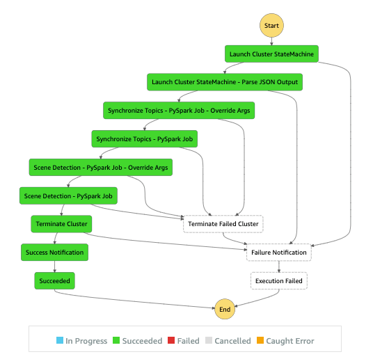
The following diagram shows a critical part of the lease processing workflow.

In this workflow, when a tenant signs a physical lease document, the property manager scans and uploads it to capture the terms electronically. A back office processor reviews the files, manually extracting key details like rent, duration, and deposit, and uses this to set up billing, payments, and reminders. The processor also manages lease functions, including processing payments, sending reminders, and issuing renewal notices, with some tasks automated but requiring manual review to address non-standard lease terms and special conditions. Alternatively, in the case when a tenant signs the lease digitally, the document is automatically captured in the system and processed further.

Overall, lease management functions involve manual and automated steps.

Solution overview

By using LLMs, you can automate key steps in the lease handling workflow, transitioning from a manual approach to a more streamlined and intelligent system. With prompt engineering, LLMs can interpret the language of lease agreements mandated by state, county, and local laws, and accurately extract terms and conditions for downstream functions such as rent processing and renewal notifications. Optionally, a fine-tuning approach helps LLMs understand industry-specific terminology.

The solution approach in this post uses Amazon Bedrock, which offers a selection of FMs and provides seamless integration with other AWS services. Although we used Anthropic’s Claude 3 Sonnet model on Amazon Bedrock to describe the solution in the post, Amazon Bedrock allows you to experiment with other models using the same approach, enabling you to find the best fit for your specific requirements.

Our event-driven solution is structured in three key steps, as illustrated in the following diagram:

Constructing a standard lease terms knowledge base – This stage involves building a comprehensive repository of standard lease terms and conditions
Validating and extracting lease agreement details – Here, we focus on accurately parsing and extracting crucial information from individual lease agreements
Automating lease-related downstream processes – The final stage implements automation for various lease management tasks and workflows

This solution demonstrates how advanced models can be effectively integrated into real-world business processes, streamlining lease management operations while maintaining accuracy and compliance.

For a practical implementation of this solution, refer to the solution repository, where you can find code for AWS Lambda functions, a sample standard lease template, and an example lease document for you to test in your own AWS environment.

Prerequisites

To implement this solution, you need the following prerequisites:

An AWS account with AWS Management Console and programmatic administrator access.
Access to Amazon Bedrock models. To demonstrate this approach, we use Anthropic’s Claude 3 Sonnet.
Access to AWS Identity and Access Management (IAM) to create roles and policies.
Proficiency in developing and deploying Lambda functions in your preferred programming language. We use Python pseudocode to describe steps in this post.
Amazon Simple Queue Service (Amazon SQS) to scale Lambda function invocations.
Access to an Amazon Simple Storage Service (Amazon S3) bucket to store standard lease templates, lease documents, and other tenant communication templates as required. You should have proficiency in setting up S3 notifications to destinations such as Lambda and Amazon SQS.
Access to Amazon DynamoDB with an understanding of your data volumes and throughput capacity mode to store lease terms extracted from lease documents.
Amazon EventBridge Scheduler to configure schedules for recurring lease-related activities.

Build a standard lease terms knowledge base

In the first stage, you build a foundation of the solution by curating a library of standard lease document templates to capture diverse laws and regulations across different states, cities, and counties.

To describe the solution approach in this post, we use the Amazon Bedrock Converse API, which provides a consistent way to invoke models, removing the complexity to adjust for model-specific differences such as inference parameters. It also manages multi-turn conversations by incorporating conversational history into requests.

With the Converse API, you can establish a centralized knowledge base in DynamoDB to streamline validation of mandatory requirements in lease documents. Because the lease templates don’t change often, a DynamoDB based knowledge base provides a cost-effective way to store mandatory terms required by different jurisdictions, removing the need to invoke Amazon Bedrock queries every time a lease is processed. The use of the Converse API with DynamoDB also eliminates an extra layer of complex knowledge base creation that requires additional integration, cost, and maintenance.

Complete the following steps to create your knowledge base:

Create an S3 bucket called Lease Templates and upload the standard lease templates.

Because lease templates don’t change often, this step is done only for new or modified templates.

Next, you configure S3 notifications to trigger a Lambda function to process the template.

Create a prompt instructing the LLM to analyze lease templates and identify terms and conditions mandated by state, county, and city regulations. The prompt can also include directives on how to parse the template and extract terms, conditions, and clauses as defined in the sample. See the following code:

<instructions>

Please review the provided residential apartment lease agreement template and extract the following information for each state or jurisdiction represented in the document. Extract state, county, city, zipcode and township details of the template in json format such as state as key and Ohio as value, zipcode as key and 43065 as value, etc. State and Zipcode is mandatory.

<laws>

Mandated state or local laws: Identify any specific laws, statutes, or regulations that the lease agreement must include or comply with based on the state or local jurisdiction. This could include things like maximum security deposit amounts, required notice periods for lease termination, or provisions tenant rights, security features on doors or windows or balcony, wall paint related obligations and landlord obligations. Provide output in json format with name and condition as key, value pairs.

</laws>

<terms>

Mandated lease terms and clauses: Extract any specific terms, clauses, or language that the lease agreement must contain due to state or local requirements. This may include items like required disclosures, prohibited provisions, or mandatory sections covering topics such as security deposits, maintenance responsibilities, or move-in/move-out procedures. Provide output in json format with name and condition as key, value pairs.

</terms>

<structure>

Formatting or structure requirements: Note if the lease agreement template must follow a particular format, structure, or organization based on state or local guidelines. This could involve the order of sections, required headings, or formatting of specific provisions. Provide output in json format with name and condition as key, value pairs.

</structure>

For each state or jurisdiction represented in the lease agreement template, please provide the extracted information in json format as described above. Include the state/jurisdiction name, the relevant mandated laws, terms, clauses, and formatting requirements. Where possible, cite the specific legal authority or source for the required provisions. The goal is to create a comprehensive guide in json format that a property manager could use to ensure their residential lease agreements comply with the applicable state and local requirements, based on the provided template document. In addition to above terms and conditions, provide any other relevant terms you find the template that could be important and should be included in lease documents by property manager. Provide only json output and don't include any other text and don't add any super header to the overall json response. Start the json with state key, value pair to put the item into Amazon DynamoDB table.

</instructions>

Using the Converse API, extract mandatory terms and conditions as JSON output with state and zipcode as unique identifiers:

doc_message = {
              "role": "user",
              "content":
[
{ "document":{"name": "Document 1",
         "format": "pdf",
         "source":{"bytes":file_bytes}}
},
{ "text": prompt
}
]
response = bedrock.converse
(
  modelId = "anthropic.claude-3-sonnet-20240229-v1:0",    
  messages = [doc_message],
  inferenceConfig = {"maxTokens":4096, "temperature":0}
)

The following screenshot shows the output of the Amazon Bedrock Converse API call, which will serve as a reference for processing lease documents for that jurisdiction.

Create a leaseagreementtemplateterms table in DynamoDB and store the JSON output, forming the knowledge base:

#Convert JSON string to Python dictionary
item = json.loads(response_text)

#Insert response_text item into DynamoDB table
table = dynamodb.Table('leaseagreementtemplateterms')
try:
response = table.put_item(Item=item)
print('Item inserted successfully: ', item['state'], item['zipcode'])
except Exception as e:
print('Error inserting item: ', item['state'], item['zipcode'], e)

You can configure on-demand or provisioned throughput capacity for the table based on your workload requirements. This data repository makes sure that the mandatory requirements for each jurisdiction are readily available for validation when new lease agreements are processed. It’s also more cost-effective to retrieve terms from the DynamoDB table than invoking Amazon Bedrock every time a lease needs to be validated against standard terms in the template.

You can repeat the process to capture standard lease terms of all jurisdictions you have operations in and if there are regulatory changes in the standard terms of already processed templates.

Validate and extract lease agreement details

In the second stage of the solution, you validate each lease agreement against standard terms captured during the previous stage to confirm compliance. After the lease is determined to be compliant on all mandatory clauses for the jurisdiction, you extract terms and conditions to run lease management functions. Compared to the volume and frequency of templates processed in first stage, you frequently process a larger number of documents in the lease processing stage, therefore a scalable solution using Amazon SQS is optimal. You can use S3 notifications and an SQS queue-based approach to decouple and scale the document processing as required.

Complete the following steps:

Create an S3 bucket called Lease Agreements to upload lease documents, and configure S3 upload notifications to destination type Amazon SQS.

Next, you configure Amazon SQS to trigger a Lambda function to perform downstream processing of the lease document.

For this post, to identify the jurisdiction, we mentioned state and zipcode as part of file name. With that information, retrieve mandatory terms corresponding to that jurisdiction from the DynamoDB leaseagreementtemplateterms knowledge base.
```
Table = dynamodb.Table('leaseagreementtemplateterms')
response = table.query(KeyConditionExpression = Key('state').eq(state) &
Key('zipcode').eq(zipcode))
```

Over a period of time, standard lease templates may change for various reasons. If you have more than one version of the template for each state and zipcode combination, use the latest version of mandatory terms for validation.

With the extracted mandatory terms and uploaded lease document, create a prompt for the Amazon Bedrock Converse API to validate whether the lease complies with all required clauses and conditions. The following prompt considers various aspects of lease processing, and you can add more details as required for your use case. The prompt also asks the LLM to score the confidence level on the accuracy of the processing, which you can use to determine if further manual review is required.

<instructions>

You are an AI data processor assisting a residential property management company. Your task is to review residential lease agreement document uploaded and validate that it contains the mandatory terms, conditions, and clauses provided in the following context.

<json_mandatory_terms>

+ str(mandatory_lease_terms_json)

</ json_mandatory_terms>

Please review the lease agreement document and check if it includes the mandatory terms, conditions, and clauses as mentioned in terms above. Do not hallucinate or use any public information for validation. Clauses could be just statements. Don't look for specific statements but make sure the meaning is in alignment.

Validate if rent amount, lease start date, security deposit amount, etc, have valid values such as amounts and dates. For example, if security deposit is mandatory in the terms JSON, then the lease document should have the term security deposit with a valid $ amount value. Identify any gaps or missing elements that are in the JSON and provide a summary report.

The report should include: The state and local jurisdiction of the property. A list of all the mandatory terms, conditions, and clauses required for that jurisdiction as per JSON. A list of any missing or incomplete elements in the lease agreement document you just reviewed. If any mandatory terms are missing or not properly mentioned with valid values in the lease document, please provide recommendations on what needs to be amended in the lease document and approximate wording for each recommendation to add in the lease document. Please provide the report in a clear and concise format that the property manager can easily understand and act upon. If all mandatory terms look good, then confirm the same in the report by outputting a response 'status: agreement is validated' along with the report. If a term or condition or clause doesn't fulfill as per mandatory JSON, then output a response 'status: agreement is not fully validated' along with the report.

<confidence_score>

Share a confidence score in percentage on how confident are you that you validation is accurate and the lease document is complete.

</confidence_score>

</instructions>

The Converse API call generates a detailed validation report in JSON format as shown in the following screenshot, outlining any sections or terms that don’t align with the mandatory requirements. It also provides a confidence score on the accuracy of the lease document and recommendations on how to amend those terms and conditions.

Based on the model’s recommendations, you can amend the lease and make sure the terms and conditions are compliant with mandatory requirements, and then re-validate the lease document.

After the document is successfully validated, the model prepares a final validation report along with a confidence score. In our solution, we’ve considered 95% as the threshold for successful validation. You can decide your threshold and have a manual review step in the workflow as required.

After the amended lease is validated successfully, prompt the Amazon Bedrock Converse API to extract required terms from the lease document, such as tenancy start date, end date, security deposit, utilities paid by, and so on. Add additional fields to the prompt as required for your business activities and workflows.

<instructions>

You are a Lease document data processor. You will be provided a lease agreement of a real estate rental unit such as apartment, home or condo. Extract the information from the lease document and create a json that can be inserted into Amazon DynamoDB table. Following are the terms and conditions of the lease that you need to extract:

state is state where the lease is processed (Example: Ohio, Pennsylvania, etc.)

zipcode is zipcode where the lease is processed (example 43065, 19019, etc.)

lease_id is Rental agreement title
new_or_amendment is 'new'
agreement_signed_date is date on which this lease is signed (mm/dd/yyyy)
deposit_amount is Deposit amount
deposit_paid_by_date is date when deposit should be paid by mm/dd/yyyy)
fixtures are kitchen appliances, furnitures or any other applicances
owner_name is Landlord's or Owner's name of the rental unit
property_address is address of the rental unit which is on lease
rent_amount is monthly rent amount
rent_paid_by_day_of_month is due date of rental payment
tenancy_end_date is lease end date on which the lease is terminating
tenancy_start_date is lease start date on which the lease is starting
tenant_name is Tenant's name of the rental unit
termination_notice_min_days is minimum notice period in days
utilities_terms_electricity is who will pay the electricity bill
When creating the summary, be sure to understand the legal language in the agreement and create a valid output.

</instructions>

Create a Lease Agreements table in DynamoDB to store the terms and condition of the lease as a lease primary record.

You can use this record to carry out lease management activities throughout the life of the lease, such as rent reminders, renewal notices, and promotional emails. Because the lease is renewed by the same tenant, you can update the primary record and extend the process. If the lease expires and a new lease is signed by different tenant, you can create a new lease primary record again for the rental unit, thereby enabling the continuous lifecycle of property management workflows.

The following screenshot is a sample lease record for each lease agreement processed in the table.

Automate lease-related notifications and reminders

After the lease terms are extracted into the lease agreement table, you can automate downstream processes. The solution in this post uses EventBridge Scheduler and Lambda functions to run different lease management functions. However, you can also use Amazon Bedrock to perform some of those functions, such as generating communications or custom notifications as required. You can determine what works best for your use case based on volumes, flexibility, and cost involved in using Amazon Bedrock and modify the approach.

Complete the following steps:

Using dates and other lease terms, configure EventBridge Scheduler to trigger periodic notifications and batch processes. For example, you can schedule monthly rent reminders or renewal notices nearing lease end or periodic promotions.

Using standard templates from Amazon S3, you can automate notices and reminders for an improved customer experience and archive the communications for future audits.

#Send rent reminder on 25th of every month using templates stored in s3
response = s3.get_object(Bucket = "leasenoticetemplates",

Key = "rentreminder.txt" )
#Publish SNS email message
topic = sns.Topic('arn:aws:sns:us-east-2:1234567890:leasecommunications')
response = topic.publish(Message = rentreminder)

The following screenshot is a sample recurring rent reminder email scheduled through EventBridge.

Conclusion

In this post, we explored a generative AI-based approach to lease processing using the power of Amazon Bedrock. Our approach addresses the complex challenges of manual lease management by establishing a comprehensive lease template library and knowledge base, automating compliance validation against jurisdiction-specific requirements, and centralizing lease term storage for efficient processing of rental management functions. This approach not only streamlines the initial processing of leases, but also significantly reduces administrative overhead in ongoing lease management. By automating lease processing activities, you can optimize administrative costs, improve accuracy, and enhance overall operational efficiency.

For the implementation of this solution, refer to the solution repository, which contains Lambda function code and sample lease files to test in your own AWS environment.

Build a dynamic rules engine with Amazon Managed Service for Apache Flink

2024-10-03 Steven Carpenter

Post Syndicated from Steven Carpenter original https://aws.amazon.com/blogs/big-data/build-a-dynamic-rules-engine-with-amazon-managed-service-for-apache-flink/

Imagine you have some streaming data. It could be from an Internet of Things (IoT) sensor, log data ingestion, or even shopper impression data. Regardless of the source, you have been tasked with acting on the data—alerting or triggering when something occurs. Martin Fowler says: “You can build a simple rules engine yourself. All you need is to create a bunch of objects with conditions and actions, store them in a collection, and run through them to evaluate the conditions and execute the actions.”

A business rules engine (or simply rules engine) is a software system that executes many rules based on some input to determine some output. Simplistically, it’s a lot of “if then,” “and,” and “or” statements that are evaluated on some data. There are many different business rule systems, such as Drools, OpenL Tablets, or even RuleBook, and they all share a commonality: they define rules (collection of objects with conditions) that get executed (evaluate the conditions) to derive an output (execute the actions). The following is a simplistic example:

if (office_temperature) < 50 degrees => send an alert

if (office_temperature) < 50 degrees AND (occupancy_sensor) == TRUE => < Trigger action to turn on heat>

When a single condition or a composition of conditions evaluates to true, it is desired to send out an alert to potentially act on that event (trigger the heat to warm the 50 degrees room).

This post demonstrates how to implement a dynamic rules engine using Amazon Managed Service for Apache Flink. Our implementation provides the ability to create dynamic rules that can be created and updated without the need to change or redeploy the underlying code or implementation of the rules engine itself. We discuss the architecture, the key services of the implementation, some implementation details that you can use to build your own rules engine, and an AWS Cloud Development Kit (AWS CDK) project to deploy this in your own account.

Solution overview

The workflow of our solution starts with the ingestion of the data. We assume that we have some source data. It could be from a variety of places, but for this demonstration, we use streaming data (IoT sensor data) as our input data. This is what we will evaluate our rules on. For example purposes, let’s assume we are looking at data from our AnyCompany Home Thermostat. We’ll see attributes like temperature, occupancy, humidity, and more. The thermostat publishes the respective values every 1 minute, so we’ll base our rules around that idea. Because we’re ingesting this data in near real time, we need a service designed specifically for this use case. For this solution, we use Amazon Kinesis Data Streams.

In a traditional rules engine, there may be a finite list of rules. The creation of new rules would likely involve a revision and redeployment of the code base, a replacement of some rules file, or some overwriting process. However, a dynamic rules engine is different. Much like our streaming input data, our rules can also be streamed as well. Here we can use Kinesis Data Streams to stream our rules as they are created.

At this point, we have two streams of data:

The raw data from our thermostat
The business rules perhaps created through a user interface

The following diagram illustrates we can connect these streams together. Architecture Diagram

Connecting streams

A typical use case for Managed Service for Apache Flink is to interactively query and analyze data in real time and continuously produce insights for time-sensitive use cases. With this in mind, if you have a rule that corresponds to the temperature dropping below a certain value (especially in winter), it might be critical to evaluate and produce a result as timely as possible.

Apache Flink connectors are software components that move data into and out of a Managed Service for Apache Flink application. Connectors are flexible integrations that let you read from files and directories. They consist of complete modules for interacting with AWS services and third-party systems. For more details about connectors, see Use Apache Flink connectors with Managed Service for Apache Flink.

We use two types of connectors (operators) for this solution:

Sources – Provide input to your application from a Kinesis data stream, file, or other data source
Sinks – Send output from your application to a Kinesis data stream, Amazon Data Firehose stream, or other data destination

Flink applications are streaming dataflows that may be transformed by user-defined operators. These dataflows form directed graphs that start with one or more sources and end in one or more sinks. The following diagram illustrates an example dataflow (source). As previously discussed, we have two Kinesis data streams that can be used as sources for our Flink program.

Flink Data Flow

The following code snippet shows how we have our Kinesis sources set up within our Flink code:

/**
* Creates a DataStream of Rule objects by consuming rule data from a Kinesis
* stream.
*
* @param env The StreamExecutionEnvironment for the Flink job
* @return A DataStream of Rule objects
* @throws IOException if an error occurs while reading Kinesis properties
*/
private DataStream<Rule> createRuleStream(StreamExecutionEnvironment env, Properties sourceProperties)
                throws IOException {
        String RULES_SOURCE = KinesisUtils.getKinesisRuntimeProperty("kinesis", "rulesTopicName");
        FlinkKinesisConsumer<String> kinesisConsumer = new FlinkKinesisConsumer<>(RULES_SOURCE,
                        new SimpleStringSchema(),
                        sourceProperties);
        DataStream<String> rulesStrings = env.addSource(kinesisConsumer)
                        .name("RulesStream")
                        .uid("rules-stream");
        return rulesStrings.flatMap(new RuleDeserializer()).name("Rule Deserialization");
}

/**
* Creates a DataStream of SensorEvent objects by consuming sensor event data
* from a Kinesis stream.
*
* @param env The StreamExecutionEnvironment for the Flink job
* @return A DataStream of SensorEvent objects
* @throws IOException if an error occurs while reading Kinesis properties
*/
private DataStream<SensorEvent> createSensorEventStream(StreamExecutionEnvironment env,
            Properties sourceProperties) throws IOException {
    String DATA_SOURCE = KinesisUtils.getKinesisRuntimeProperty("kinesis", "dataTopicName");
    FlinkKinesisConsumer<String> kinesisConsumer = new FlinkKinesisConsumer<>(DATA_SOURCE,
                    new SimpleStringSchema(),
                    sourceProperties);
    DataStream<String> transactionsStringsStream = env.addSource(kinesisConsumer)
                    .name("EventStream")
                    .uid("sensor-events-stream");

    return transactionsStringsStream.flatMap(new JsonDeserializer<>(SensorEvent.class))
                    .returns(SensorEvent.class)
                    .flatMap(new TimeStamper<>())
                    .returns(SensorEvent.class)
                    .name("Transactions Deserialization");
}

We use a broadcast state, which can be used to combine and jointly process two streams of events in a specific way. A broadcast state is a good fit for applications that need to join a low-throughput stream and a high-throughput stream or need to dynamically update their processing logic. The following diagram illustrates an example how the broadcast state is connected. For more details, see A Practical Guide to Broadcast State in Apache Flink.

Broadcast State

This fits the idea of our dynamic rules engine, where we have a low-throughput rules stream (added to as needed) and a high-throughput transactions stream (coming in at a regular interval, such as one per minute). This broadcast stream allows us to take our transactions stream (or the thermostat data) and connect it to the rules stream as shown in the following code snippet:

// Processing pipeline setup
DataStream<Alert> alerts = sensorEvents
    .connect(rulesStream)
    .process(new DynamicKeyFunction())
    .uid("partition-sensor-data")
    .name("Partition Sensor Data by Equipment and RuleId")
    .keyBy((equipmentSensorHash) -> equipmentSensorHash.getKey())
    .connect(rulesStream)
    .process(new DynamicAlertFunction())
    .uid("rule-evaluator")
    .name("Rule Evaluator");

To learn more about the broadcast state, see The Broadcast State Pattern. When the broadcast stream is connected to the data stream (as in the preceding example), it becomes a BroadcastConnectedStream. The function applied to this stream, which allows us to process the transactions and rules, implements the processBroadcastElement method. The KeyedBroadcastProcessFunction interface provides three methods to process records and emit results:

processBroadcastElement() – This is called for each record of the broadcasted stream (our rules stream).
processElement() – This is called for each record of the keyed stream. It provides read-only access to the broadcast state to prevent modifications that result in different broadcast states across the parallel instances of the function. The processElement method retrieves the rule from the broadcast state and the previous sensor event of the keyed state. If the expression evaluates to TRUE (discussed in the next section), an alert will be emitted.
onTimer() – This is called when a previously registered timer fires. Timers can be registered in the processElement method and are used to perform computations or clean up states in the future. This is used in our code to make sure any old data (as defined by our rule) is evicted as necessary.

We can handle the rule in the broadcast state instance as follows:

@Override
public void processBroadcastElement(Rule rule, Context ctx, Collector<Alert> out) throws Exception {
   BroadcastState<String, Rule> broadcastState = ctx.getBroadcastState(RulesEvaluator.Descriptors.rulesDescriptor);
   Long currentProcessTime = System.currentTimeMillis();
   // If we get a new rule, we'll give it insufficient data rule op status
    if (!broadcastState.contains(rule.getId())) {
        outputRuleOpData(rule, OperationStatus.INSUFFICIENT_DATA, currentProcessTime, ctx);
    }
   ProcessingUtils.handleRuleBroadcast(rule, broadcastState);
}

static void handleRuleBroadcast(FDDRule rule, BroadcastState<String, FDDRule> broadcastState)
        throws Exception {
    switch (rule.getStatus()) {
        case ACTIVE:
            broadcastState.put(rule.getId(), rule);
            break;
        case INACTIVE:
            broadcastState.remove(rule.getId());
            break;
    }
}

Notice what happens in the code when the rule status is INACTIVE. This would remove the rule from the broadcast state, which would then no longer consider the rule to be used. Similarly, handling the broadcast of a rule that is ACTIVE would add or replace the rule within the broadcast state. This is allowing us to dynamically make changes, adding and removing rules as necessary.

Evaluating rules

Rules can be evaluated in a variety of ways. Although it’s not a requirement, our rules were created in a Java Expression Language (JEXL) compatible format. This allows us to evaluate rules by providing a JEXL expression along with the appropriate context (the necessary transactions to reevaluate the rule or key-value pairs), and simply calling the evaluate method:

JexlExpression expression = jexl.createExpression(rule.getRuleExpression());
Boolean isAlertTriggered = (Boolean) expression.evaluate(context);

A powerful feature of JEXL is that not only can it support simple expressions (such as those including comparison and arithmetic), it also has support for user-defined functions. JEXL allows you to call any method on a Java object using the same syntax. If there is a POJO with the name SENSOR_cebb1baf_2df0_4267_b489_28be562fccea that has the method hasNotChanged, you would call that method using the expression. You can find more of these user-defined functions that we used within our SensorMapState class.

Let’s look at an example of how this would work, using a rule expression exists that reads as follows:

"SENSOR_cebb1baf_2df0_4267_b489_28be562fccea.hasNotChanged(5)"

This rule, evaluated by JEXL, would be equivalent to a sensor that hasn’t changed in 5 minutes

The corresponding user-defined function (part of SensorMapState) that is exposed to JEXL (using the context) is as follows:

public Boolean hasNotChanged(Integer time) {
    Long minutesSinceChange = getMinutesSinceChange();
    log.debug("Time: " + time + " | Minutes since change: " + minutesSinceChange);
    return minutesSinceChange >  time;
}

Relevant data, like that below, would go into the context window, which would then be used to evaluate the rule.

{
    "id": "SENSOR_cebb1baf_2df0_4267_b489_28be562fccea",
    "measureValue": 10,
    "eventTimestamp": 1721666423000
}

In this case, the result (or value of isAlertTriggered) is TRUE.

Creating sinks

Much like how we previously created sources, we also can create sinks. These sinks will be used as the end to our stream processing where our analyzed and evaluated results will get emitted for future use. Like our source, our sink is also a Kinesis data stream, where a downstream Lambda consumer will iterate the records and process them to take the appropriate action. There are many applications of downstream processing; for example, we can persist this evaluation result, create a push notification, or update a rule dashboard.

Based on the previous evaluation, we have the following logic within the process function itself:

if (isAlertTriggered) {
    alert = new Alert(rule.getEquipmentName(), rule.getName(), rule.getId(), AlertStatus.START,
            triggeringEvents, currentEvalTime);
    log.info("Pushing {} alert for {}", AlertStatus.START, rule.getName());
}
out.collect(alert);

When the process function emits the alert, the alert response is sent to the sink, which then can be read and used downstream in the architecture:

alerts.flatMap(new JsonSerializer<>(Alert.class))
    .name("Alerts Deserialization").sinkTo(createAlertSink(sinkProperties))
    .uid("alerts-json-sink")
    .name("Alerts JSON Sink");

At this point, we can then process it. We have a Lambda function logging the records where we can see the following:

{
   "equipmentName":"THERMOSTAT_1",
   "ruleName":"RuleTest2",
   "ruleId":"cda160c0-c790-47da-bd65-4abae838af3b",
   "status":"START",
   "triggeringEvents":[
      {
         "equipment":{
            "id":"THERMOSTAT_1",
         },
         "id":"SENSOR_cebb1baf_2df0_4267_b489_28be562fccea",
         "measureValue":20.0,
         "eventTimestamp":1721672715000,
         "ingestionTimestamp":1721741792958
      }
   ],
   "timestamp":1721741792790
}

Although simplified in this example, these code snippets form the basis for taking the evaluation results and sending them elsewhere.

Conclusion

In this post, we demonstrated how to implement a dynamic rules engine using Managed Service for Apache Flink with both the rules and input data streamed through Kinesis Data Streams. You can learn more about it with the e-learning that we have available.

As companies seek to implement near real-time rules engines, this architecture presents a compelling solution. Managed Service for Apache Flink offers powerful capabilities for transforming and analyzing streaming data in real time, while simplifying the management of Flink workloads and seamlessly integrating with other AWS services.

To help you get started with this architecture, we’re excited to announce that we’ll be publishing our complete rules engine code as a sample on GitHub. This comprehensive example will go beyond the code snippets provided in our post, offering a deeper look into the intricacies of building a dynamic rules engine with Flink.

We encourage you to explore this sample code, adapt it to your specific use case, and take advantage of the full potential of real-time data processing in your applications. Check out the GitHub repository, and don’t hesitate to reach out with any questions or feedback as you embark on your journey with Flink and AWS!

About the Authors

Steven Carpenter is a Senior Solution Developer on the AWS Industries Prototyping and Customer Engineering (PACE) team, helping AWS customers bring innovative ideas to life through rapid prototyping on the AWS platform. He holds a master’s degree in Computer Science from Wayne State University in Detroit, Michigan. Connect with Steven on LinkedIn!

Aravindharaj Rajendran is a Senior Solution Developer within the AWS Industries Prototyping and Customer Engineering (PACE) team, based in Herndon, VA. He helps AWS customers materialize their innovative ideas by rapid prototyping using the AWS platform. Outside of work, he loves playing PC games, Badminton and Traveling.

Automatically replicate your card payment keys across AWS Regions

2024-08-30 Ruy Cavalcanti

Post Syndicated from Ruy Cavalcanti original https://aws.amazon.com/blogs/security/automatically-replicate-your-card-payment-keys-across-aws-regions/

In this blog post, I dive into a cross-Region replication (CRR) solution for card payment keys, with a specific focus on the powerful capabilities of AWS Payment Cryptography, showing how your card payment keys can be securely transported and stored.

In today’s digital landscape, where online transactions have become an integral part of our daily lives, ensuring the seamless operation and security of card payment transactions is of utmost importance. As customer expectations for uninterrupted service and data protection continue to rise, organizations are faced with the challenge of implementing robust security measures and disaster recovery strategies that can withstand even the most severe disruptions.

For large enterprises dealing with card payments, the stakes are even higher. These organizations often have stringent requirements related to disaster recovery (DR), resilience, and availability, where even a 99.99 percent uptime isn’t enough. Additionally, because these enterprises deliver their services globally, they need to ensure that their payment applications and the associated card payment keys, which are crucial for securing card data and payment transactions, are securely replicated and stored across AWS Regions.

Furthermore, I explore an event-driven, serverless architecture and the use of AWS PrivateLink to securely move keys through the AWS backbone, providing additional layers of security and efficiency. Overall, this blog post offers valuable insights into using AWS services for secure and resilient data management across AWS Regions.

Card payment key management

If you examine key management, you will notice that card payment keys are shared between devices and third parties today the same as they were around 40 years ago.

A key ceremony is the process held when parties want to securely exchange keys. It involves key custodians responsible for transporting and entering, key components that have been printed on pieces of paper into a hardware security module (HSM). This is necessary to share initial key encryption keys.

Let’s look at the main issues with the current key ceremony process:

It requires a secure room with a network-disconnected Payment HSM
The logistics are difficult: Three key custodians in the same place at the same time
Timewise, it usually takes weeks to have all custodians available, which can interfere with a project release
The cost of the operation which includes maintaining a secure room and the travel of the key custodians
Lost or stolen key components

Now, let’s consider the working keys used to encrypt sensitive card data. They rely on those initial keys to protect them. If the initial keys are compromised, their associated working keys are also considered compromised. I also see companies using key management standards from the 1990s, such as ANSI X9.17 / FIPS 171, to share working keys. NIST withdrew the FIPS 171 standard in 2005.

Analyzing the current scenario, you’ll notice security risks because of the way keys are shared today and sometimes because organizations are using deprecated standards.

So, let’s get card payment security into the twenty-first century!

Solution overview

AWS Payment Cryptography is a highly available and scalable service that currently operates within the scope of an individual Region. This means that the encryption keys and associated metadata are replicated across multiple Availability Zones within that Region, providing redundancy and minimizing the risk of downtime caused by failures within a single Region.

While this regional replication across multiple Availability Zones provides a higher level of availability and fault tolerance compared to traditional on-premises HSM solutions, some customers with stringent business continuity requirements have requested support for multi-Region replication.

By spanning multiple Regions, organizations can achieve a higher level of resilience and disaster recovery capabilities because data and services can be replicated and failover mechanisms can be implemented across geographically dispersed locations.

This Payment Cryptography CRR solution addresses the critical requirements of high availability, resilience, and disaster recovery for card payment transactions. By replicating encryption keys and associated metadata across multiple Regions, you can maintain uninterrupted access to payment services, even in the event of a regional outage or disaster.

Note: When planning your replication strategy, check the available Payment Cryptography service endpoints.

Here’s how it works:

Primary Region: Encryption keys are generated and managed in a primary Region using Payment Cryptography.
Replication: The generated encryption keys are securely replicated to a secondary Region, creating redundant copies for failover purposes.
Failover: In the event of a regional outage or disaster in the primary Region, payment operations can seamlessly failover to a secondary Region, using the replicated encryption keys to continue processing transactions without interruption.

This cross-Region replication approach enhances availability and resilience and facilitates robust disaster recovery strategies, allowing organizations to quickly restore payment services in a new Region if necessary.

Figure 1: Cross-Region replication (CRR) solution architecture

The elements of the CRR architecture are as follows:

Payment Cryptography control plane events are sent to an AWS CloudTrail trail.
The CloudTrail trail is configured to send logs to an Amazon CloudWatch Logs log group.
This log group contains an AWS Lambda subscription filter that filters the following events from Payment Cryptography: CreateKey, DeleteKey and ImportKey.
When one of the events is detected, a Lambda function is launched to start key replication.
The Lambda function performs key export and import processes in a secure way using TR-31, which uses an initial key securely generated and shared using TR-34. This initial key is generated when the solution is enabled.
Communication between the primary (origin) Region and the Payment Cryptography service endpoint at the secondary (destination) Region is done through an Amazon Virtual Private Cloud (Amazon VPC) peering connection, over VPC interface endpoints from PrivateLink.
Metadata information is saved on Amazon DynamoDB tables.

Walkthrough

The CRR solution is deployed in several steps, and it’s essential to understand the underlying processes involved, particularly TR-34 (ANSI X9.24-2) and TR-31 (ANSI X9.143-2022), which play crucial roles in ensuring the secure replication of card payment keys across Regions.

Clone the solution repository from GitHub.
Verify that the prerequisites are in place.
Define which Region the AWS Cloud Development Kit (AWS CDK) stack will be deployed in. This is the primary Region that Payment Cryptography keys will be replicated from.
Enable CRR. This step involves the TR-34 process, which is a widely adopted standard for the secure distribution of symmetric keys using asymmetric techniques. In the context of this solution, TR-34 is used to securely exchange the initial key-encrypting key (KEK) between the primary and secondary Regions. This KEK is then used to encrypt and securely transmit the card payment keys (also called working keys) during the replication process. TR-34 uses asymmetric cryptographic algorithms, such as RSA, to maintain the confidentiality, integrity and authenticity of the exchanged keys.

Figure 2: TR-34 import key process
Create, import, and delete keys in the primary Region to check that keys will be automatically replicated. This step uses the TR-31 process, which is a standard for the secure exchange of cryptographic keys and related data. In this solution, TR-31 is employed to securely replicate the card payment keys from the primary Region to the secondary Region, using the previously established KEK for encryption. TR-31 incorporates various cryptographic algorithms, such as AES and HMAC, to protect the confidentiality and integrity of the replicated keys during transit

Figure 3: TR-31 import key process
Clean up when needed.

Detailed information about key blocks can be found on the related ANSI documentation. To summarize, the TR-31 key block specification and the TR-34 key block specification, which is based on the TR-31 key block specification, consists of three parts:

Key block header (KBH) – Contains attribute information about the key and the key block.
Encrypted data – This is the key (initial key encryption key for TR-34 and working key for TR-31) being exchanged.
Signature (MAC) – Calculated over the KBH and encrypted data.

Figure 4 presents the entire TR-31 and TR-34 key block parts. It is also called key binding method, which is the technique used to protect the key block secrecy and integrity. On both key blocks, the key, its length, and padding fields are encrypted, maintaining the key block secrecy. Signing of the entire key block fields verifies its integrity and authenticity. The signed result is appended to the end of the block.

Figure 4: TR-31 and TR-34 key block formats

By adhering to industry-standard protocols like TR-34 and TR-31, this solution helps to ensure that the replication of card payment keys across Regions is performed in a secure manner that delivers confidentiality, integrity, and authenticity. It’s worth mentioning that Payment Cryptography fully supports and implements these standards, providing a solution that adheres to PCI standards for secure key management and replication.

If you want to dive deep into this key management processes, see the service documentation page on import and export keys.

Prerequisites

The Payment Cryptography CRR solution will be deployed through the AWS CDK. The code was developed in Python and assumes that there is a python3 executable in your path. It’s also assumed that the AWS Command Line Interface (AWS CLI) and AWS CDK executables exist in the path system variable of your local computer.

Download and install the following:

It’s recommended that you use the latest stable versions. Tests were performed using the following versions:

Python: 3.12.2 (MacOS version)
jq: 1.7.1 (MacOS version)
AWS CLI: aws-cli/2.15.29 Python/3.11.8 Darwin/22.6.0 exe/x86_64 prompt/off
AWS CDK: 2.132.1 (build 9df7dd3)

To set up access to your AWS account, see Configure the AWS CLI.

Note: Tests and commands in the following sections where run on a MacOS operating system.

Deploy the primary resources

The solution is deployed in two main parts:

Primary Region resources deployment
CRR setup, where a secondary Region is defined for deployment of the necessary resources

This section will cover the first part:

Figure 5: Primary Region resources

Figure 5 shows the resources that will be deployed in the primary Region:

A CloudTrail trail for write-only log events.
CloudWatch Logs log group associated with the CloudTrail trail. An Amazon Simple Storage Service (Amazon S3) bucket is also created to store this trail’s log events.
A VPC, private subnets, a security group, Lambda functions, and VPC endpoint resources to address private communication inside the AWS backbone.
DynamoDB tables and DynamoDB Streams to manage key replication and orchestrate the solution deployment to the secondary Region.
Lambda functions responsible for managing and orchestrating the solution deployment and setup.

Some parameters can be configured before deployment. They’re located in the cdk.json file (part of the GitHub solution to be downloaded) inside the solution base directory.

The parameters reside inside the context.ENVIRONMENTS.dev key:

{
  ...
  "context": {
    ...
    "ENVIRONMENTS": {
      "dev": {
        "origin_vpc_cidr": "10.2.0.0/16",
        "origin_vpc_name": "origin-vpc",
        "origin_subnets_mask": 22,
        "origin_subnets_prefix_name": "origin-subnet-private"
      }
    }
  }
}

Note: You can change the parameters origin_vpc_cidr, origin_vpc_name and origin_subnets_prefix_name.

Validate that there aren’t VPCs already created with the same CIDR range as the one defined in this file. Currently, the solution is set to be deployed in only two Availability Zones, so the suggestion is to keep the origin_subnet_mask value as is.

To deploy the primary resources:

Download the solution folder from GitHub:

$ git clone https://github.com/aws-samples/automatically-replicate-your-card-payment-keys.git && cd automatically-replicate-your-card-payment-keys

Inside the solution directory, create a python virtual environment:
```
$ python3 -m venv .venv
```
Activate the python virtual environment:
```
$ source .venv/bin/activate
```
Install the dependencies:
```
$ pip install -r requirements.txt
```
If this is the first time deploying resources with the AWS CDK to your account in the selected AWS Region, run:
```
$ cdk bootstrap
```

Deploy the solution using the AWS CDK:

$ cdk deploy

Expected output:

Do you wish to deploy these changes (y/n)? y  
apc-crr: deploying... [1/1]  
apc-crr: creating CloudFormation changeset...
   apc-crr
  Deployment time: 307.88s
Stack ARN:
arn:aws:cloudformation:<aws_region>:<aws_account>:stack/apc-crr/<stack_id>
  Total time: 316.06s

If the solution is correctly deployed, an AWS CloudFormation stack with the name apc-crr will have a status of CREATE_COMPLETE status. You can check that by running the following command:

$ aws cloudformation list-stacks --stack-status CREATE_COMPLETE

Expected output:

{
    "StackSummaries": [
        {
            "StackId": "arn:aws:cloudformation:us-east-1:111122223333:stack/apc-crr/5933bc00-f5c1-11ee-9bb2-12ef8d00991b",
            "StackName": "apc-crr",
            "CreationTime": "2024-04-08T16:02:07.413000+00:00",
            "LastUpdatedTime": "2024-04-08T16:02:21.439000+00:00",
            "StackStatus": "CREATE_COMPLETE",
            "DriftInformation": {
                "StackDriftStatus": "NOT_CHECKED"
            }
        },
        {
            "StackId": "arn:aws:cloudformation:us-east-1:111122223333:stack/CDKToolkit/781e5390-e528-11ee-823a-0a6d63bbc467",
            "StackName": "CDKToolkit",
            "TemplateDescription": "This stack includes resources needed to deploy AWS CDK apps into this environment",
            "CreationTime": "2024-03-18T13:07:27.472000+00:00",
            "LastUpdatedTime": "2024-03-18T13:07:35.060000+00:00",
            "StackStatus": "CREATE_COMPLETE",
            "DriftInformation": {
                "StackDriftStatus": "NOT_CHECKED"
            }
        }
    ]
}

Set up cross-Region replication

Some parameters can be configured before initiating the setup. They’re located in the enable-crr.json file in the ./application folder.

The contents of the enable-crr.json file are:

{
  "enabled": true,
  "dest_region": "us-east-1",
  "kek_alias": "CRR_KEK_DO-NOT-DELETE_",
  "key_algo": "TDES_3KEY",
  "kdh_alias": "KDH_SIGN_KEY_DO-NOT-DELETE_",
  "krd_alias": "KRD_SIGN_KEY_DO-NOT-DELETE_",
  "dest_vpc_name": "apc-crr/destination-vpc",
  "dest_vpc_cidr": "10.3.0.0/16",
  "dest_subnet1_cidr": "10.3.0.0/22",
  "dest_subnet2_cidr": "10.3.4.0/22",
  "dest_subnets_prefix_name": "apc-crr/destination-vpc/destination-subnet-private",
  "dest_rt_prefix_name": "apc-crr/destination-vpc/destination-rtb-private"
}

You can change the dest_region, dest_vpc_name, dest_vpc_cidr, dest_subnet1_cidr, dest_subnet2_cidr, dest_subnets_prefix_name and dest_rt_prefix_name parameters.

Validate that there are no VPCs or subnets already created with the same CIDR ranges as are defined in this file.

To enable CRR and monitor its deployment process

Enable CRR.

From the solution base folder, navigate to the application directory:

$ cd application

Run the enable script.

$ ./enable-crr.sh

Expected output:

START RequestId: 8aad062a-ff0b-4963-8ca0-f8078346854f Version: $LATEST  
Setup has initiated. A CloudFormation template will be deployed in us-west-2.  
Please check the apcStackMonitor log to follow the deployment status.  
You can do that by checking the CloudWatch Logs Log group /aws/apc-crr/apcStackMonitor in the Management Console,  
or by typing on a shell terminal: aws logs tail "/aws/lambda/apcStackMonitor" --follow  
You can also check the CloudFormation Stack in the Management Console: Account 111122223333, Region us-west-2  
END RequestId: 8aad062a-ff0b-4963-8ca0-f8078346854f  
REPORT RequestId: 8aad062a-ff0b-4963-8ca0-f8078346854f  Duration: 1484.53 ms  Billed Duration: 1485 ms  Memory Size: 128 MB Max Memory Used: 79 MB  Init Duration: 400.95 ms

This will launch a CloudFormation stack to be deployed in the AWS Region that the keys will be replicated to (secondary Region). Logs will be presented in the /aws/lambda/apcStackMonitor log (terminal from step 2).

If the stack is successfully deployed (CREATE_COMPLETE state), then the KEK setup will be invoked. Logs will be presented in the /aws/lambda/apcKekSetup log (terminal from step 3).

If the following message is displayed in the apcKekSetup log, then it means that the setup was concluded and new working keys created, deleted, or imported will be replicated.

Keys Generated, Imported and Deleted in <Primary (Origin) Region> are now being automatically replicated to <Secondary (Destination) Region>

There should be two keys created in the Region where CRR is deployed and two keys created where the working keys will be replicated. Use the following commands to check the keys:

$ aws payment-cryptography list-keys --region us-east-1

Command output showing the keys generated in the primary Region (us-east-1 in the example):

{
    "Keys": [
        {
            "Enabled": true,
            "KeyArn": "arn:aws:payment-cryptography:us-east-1:111122223333:key/oevdxprw6szesmfx",
            "KeyAttributes": {
                "KeyAlgorithm": "RSA_4096",
                "KeyClass": "PUBLIC_KEY",
                "KeyModesOfUse": {
                    "Decrypt": false,
                    "DeriveKey": false,
                    "Encrypt": false,
                    "Generate": false,
                    "NoRestrictions": false,
                    "Sign": false,
                    "Unwrap": false,
                    "Verify": true,
                    "Wrap": false
                },
                "KeyUsage": "TR31_S0_ASYMMETRIC_KEY_FOR_DIGITAL_SIGNATURE"
            },
            "KeyState": "CREATE_COMPLETE"
        },
        {
            "Enabled": true,
            "Exportable": true,
            "KeyArn": "arn:aws:payment-cryptography:us-east-1:111122223333:key/ey63g3an7u4ifz7u",
            "KeyAttributes": {
                "KeyAlgorithm": "TDES_3KEY",
                "KeyClass": "SYMMETRIC_KEY",
                "KeyModesOfUse": {
                    "Decrypt": true,
                    "DeriveKey": false,
                    "Encrypt": true,
                    "Generate": false,
                    "NoRestrictions": false,
                    "Sign": false,
                    "Unwrap": true,
                    "Verify": false,
                    "Wrap": true
                },
                "KeyUsage": "TR31_K0_KEY_ENCRYPTION_KEY"
            },
            "KeyCheckValue": "7FB069",
            "KeyState": "CREATE_COMPLETE"
        }
    ]
}

$ aws payment-cryptography list-keys --region us-west-2

The following is the command output showing the keys generated in the secondary Region (us-west-2 in the example):

{
    "Keys": [
        {
            "Enabled": true,
            "Exportable": true,
            "KeyArn": "arn:aws:payment-cryptography:us-west-2:111122223333:key/4luahnz4ubuioq4s",
            "KeyAttributes": {
                "KeyAlgorithm": "RSA_2048",
                "KeyClass": "ASYMMETRIC_KEY_PAIR",
                "KeyModesOfUse": {
                    "Decrypt": true,
                    "DeriveKey": false,
                    "Encrypt": true,
                    "Generate": false,
                    "NoRestrictions": false,
                    "Sign": false,
                    "Unwrap": true,
                    "Verify": false,
                    "Wrap": true
                },
                "KeyUsage": "TR31_D1_ASYMMETRIC_KEY_FOR_DATA_ENCRYPTION"
            },
            "KeyCheckValue": "56739D06",
            "KeyState": "CREATE_COMPLETE"
        },
        {
            "Enabled": true,
            "Exportable": true,
            "KeyArn": "arn:aws:payment-cryptography:us-west-2:111122223333:key/5gao3i6qvuyqqtzk",
            "KeyAttributes": {
                "KeyAlgorithm": "TDES_3KEY",
                "KeyClass": "SYMMETRIC_KEY",
                "KeyModesOfUse": {
                    "Decrypt": true,
                    "DeriveKey": false,
                    "Encrypt": true,
                    "Generate": false,
                    "NoRestrictions": false,
                    "Sign": false,
                    "Unwrap": true,
                    "Verify": false,
                    "Wrap": true
                },
                "KeyUsage": "TR31_K0_KEY_ENCRYPTION_KEY"
            },
            "KeyCheckValue": "7FB069",
            "KeyState": "CREATE_COMPLETE"
        }
    ]
}

Monitor the resources deployment in the secondary Region. Open a terminal to tail the apcStackMonitor Lambda log and check the deployment of the resources in the secondary Region.

$ aws logs tail "/aws/lambda/apcStackMonitor" --follow

The expected output is:

2024-03-05T15:18:17.870000+00:00 2024/03/05/apcStackMonitor[$LATEST]6e6762b029cb4f7d8963c3206226deac INIT_START Runtime Version: python:3.11.v29  Runtime Version ARN: arn:aws:lambda:us-east-1::runtime:2fb93380dac14772d30092f109b1784b517398458eef71a3f757425231fe6769  
2024-03-05T15:18:18.321000+00:00 2024/03/05/apcStackMonitor[$LATEST]6e6762b029cb4f7d8963c3206226deac START RequestId: 1bdd37b4-e95b-43bd-a49b-9da55e603845 Version: $LATEST  
2024-03-05T15:18:18.933000+00:00 2024/03/05/apcStackMonitor[$LATEST]6e6762b029cb4f7d8963c3206226deac Stack creation in progress. Status: CREATE_IN_PROGRESS  
2024-03-05T15:18:24.017000+00:00 2024/03/05/apcStackMonitor[$LATEST]6e6762b029cb4f7d8963c3206226deac Stack creation in progress. Status: CREATE_IN_PROGRESS  
2024-03-05T15:18:29.108000+00:00 2024/03/05/apcStackMonitor[$LATEST]6e6762b029cb4f7d8963c3206226deac Stack creation in progress. Status: CREATE_IN_PROGRESS  
...  
2024-03-05T15:21:32.302000+00:00 2024/03/05/apcStackMonitor[$LATEST]6e6762b029cb4f7d8963c3206226deac Stack creation in progress. Status: CREATE_IN_PROGRESS  
2024-03-05T15:21:37.390000+00:00 2024/03/05/apcStackMonitor[$LATEST]6e6762b029cb4f7d8963c3206226deac Stack creation completed. Status: CREATE_COMPLETE  
2024-03-05T15:21:38.258000+00:00 2024/03/05/apcStackMonitor[$LATEST]6e6762b029cb4f7d8963c3206226deac Stack successfully deployed. Status: CREATE_COMPLETE  
2024-03-05T15:21:38.354000+00:00 2024/03/05/apcStackMonitor[$LATEST]6e6762b029cb4f7d8963c3206226deac END RequestId: 1bdd37b4-e95b-43bd-a49b-9da55e603845  
2024-03-05T15:21:38.354000+00:00 2024/03/05/apcStackMonitor[$LATEST]6e6762b029cb4f7d8963c3206226deac REPORT RequestId: 1bdd37b4-e95b-43bd-a49b-9da55e603845Duration: 200032.11 ms Billed Duration: 200033 ms  Memory Size: 128 MB Max Memory Used: 93 MB  Init Duration: 450.87 ms

Monitor the setup of the KEKs between the primary and secondary Regions. Open another terminal to tail the apcKekSetup Lambda log and check the setup of the KEK between the key distribution host (Payment Cryptography in the primary Region) and the key receiving devices (Payment Cryptography in the secondary Region).

This process uses the TR-34 norm.

$ aws logs tail "/aws/lambda/apcKekSetup" -–follow

The expected output is:

2024-03-12T14:58:18.954000+00:00 2024/03/12/apcKekSetup[$LATEST]ea4c6a7c85ac42da8a043aa8626d2897 INIT_START Runtime Version: python:3.11.v29  Runtime Version ARN: arn:aws:lambda:us-west-2::runtime:2fb93380dac14772d30092f109b1784b517398458eef71a3f757425231fe6769  
2024-03-12T14:58:19.399000+00:00 2024/03/12/apcKekSetup[$LATEST]ea4c6a7c85ac42da8a043aa8626d2897 START RequestId: a9b60171-dfaf-433a-954c-b0a332d22f50 Version: $LATEST  
2024-03-12T14:58:19.596000+00:00 2024/03/12/apcKekSetup[$LATEST]ea4c6a7c85ac42da8a043aa8626d2897 ##### Step 1. Generating Key Encryption Key (KEK) - Key that will be used to encrypt the Working Keys  
2024-03-12T14:58:19.850000+00:00 2024/03/12/apcKekSetup[$LATEST]ea4c6a7c85ac42da8a043aa8626d2897 ##### Step 2. Getting APC Import Parameters from us-east-1  
2024-03-12T14:58:21.680000+00:00 2024/03/12/apcKekSetup[$LATEST]ea4c6a7c85ac42da8a043aa8626d2897 ##### Step 3. Importing the Root Wrapping Certificates in us-west-2  
2024-03-12T14:58:21.826000+00:00 2024/03/12/apcKekSetup[$LATEST]ea4c6a7c85ac42da8a043aa8626d2897 ##### Step 4. Getting APC Export Parameters from us-west-2  
2024-03-12T14:58:23.193000+00:00 2024/03/12/apcKekSetup[$LATEST]ea4c6a7c85ac42da8a043aa8626d2897 ##### Step 5. Importing the Root Signing Certificates in us-east-1  
2024-03-12T14:58:23.439000+00:00 2024/03/12/apcKekSetup[$LATEST]ea4c6a7c85ac42da8a043aa8626d2897 ##### Step 6. Exporting the KEK from us-west-2  
2024-03-12T14:58:23.555000+00:00 2024/03/12/apcKekSetup[$LATEST]ea4c6a7c85ac42da8a043aa8626d2897 ##### Step 7. Importing the Wrapped KEK to us-east-1  
2024-03-12T14:58:23.840000+00:00 2024/03/12/apcKekSetup[$LATEST]ea4c6a7c85ac42da8a043aa8626d2897 ##### Initial Key Exchange Successfully Completed.  
2024-03-12T14:58:23.840000+00:00 2024/03/12/apcKekSetup[$LATEST]ea4c6a7c85ac42da8a043aa8626d2897 Keys Generated, Imported and Deleted in us-west-2 are now being automatically replicated to us-east-1  
2024-03-12T14:58:23.840000+00:00 2024/03/12/apcKekSetup[$LATEST]ea4c6a7c85ac42da8a043aa8626d2897 Keys already present in APC won't be replicated. If you want to, it must be done manually.  
2024-03-12T14:58:23.844000+00:00 2024/03/12/apcKekSetup[$LATEST]ea4c6a7c85ac42da8a043aa8626d2897 END RequestId: a9b60171-dfaf-433a-954c-b0a332d22f50  
2024-03-12T14:58:23.844000+00:00 2024/03/12/apcKekSetup[$LATEST]ea4c6a7c85ac42da8a043aa8626d2897 REPORT RequestId: a9b60171-dfaf-433a-954c-b0a332d22f50 Duration: 4444.78 ms  Billed Duration: 4445 ms  Memory Size: 5120 MB  Max Memory Used: 95 MB  Init Duration: 444.73 ms

Testing

Now it’s time to test the solution. The idea is to simulate an application that manages keys in the service. You will use AWS CLI to send commands directly from a local computer to the Payment Cryptography public endpoints.

Check if the user or role being used has the necessary permissions to manage keys in the service. The following AWS Identity and Access Management (IAM) policy example shows an IAM policy that can be attached to the user or role that will run the commands in the service.

{
      "Version": "2012-10-17",
      "Statement": [
            {
               "Effect": "Allow",
               "Action": [
                  "payment-cryptography:CreateKey",
                  "payment-cryptography:ImportKey",
                  "payment-cryptography:DeleteKey"
               ],
               "Resource": [
                  "*"
               ]
            }   
      ]
   }

Note: As an add-on, you can change the *(asterisk) to the Amazon Resource Name (ARN) of the created key.

For information about IAM policies, see the Identity and access management for Payment Cryptography documentation.

To test the solution

Prepare to monitor the replication processes. Open a new terminal to monitor the apcReplicateWk log and verify that keys are being replicated from one Region to the other.
```
$ aws logs tail "/aws/lambda/apcReplicateWk" --follow
```

Create, import, and delete working keys. Start creating and deleting keys in the account and Region where the CRR solution was deployed (primary Region).

Currently, the solution only listens to the CreateKey, ImportKey and DeleteKey commands. CreateAlias and DeleteAlias commands aren’t yet implemented, so the aliases won’t replicate.

It takes some time for the replication function to be invoked because it relies on the following steps:

A Payment Cryptography (CreateKey, ImportKey, or DeleteKey) log event is delivered to a CloudTrail trail.
The log event is sent to the CloudWatch Logs log group, which invokes the subscription filter and the Lambda function associated with it is run.

CloudTrail typically delivers logs within about 5 minutes of an API call. This time isn’t guaranteed. See the AWS CloudTrail Service Level Agreement for more information.

Example 1: Create a working key

Run the following command:

aws payment-cryptography create-key --exportable --key-attributes KeyAlgorithm=TDES_2KEY,\
KeyUsage=TR31_C0_CARD_VERIFICATION_KEY,KeyClass=SYMMETRIC_KEY, \
KeyModesOfUse='{Generate=true,Verify=true}'

Command output:

{
    "Key": {
        "CreateTimestamp": "2022-10-26T16:04:11.642000-07:00",
        "Enabled": true,
        "Exportable": true,
        "KeyArn": "arn:aws:payment-cryptography:us-east-1:111122223333:key/hjprdg5o4jtgs5tw",
        "KeyAttributes": {
            "KeyAlgorithm": "TDES_2KEY",
            "KeyClass": "SYMMETRIC_KEY",
            "KeyModesOfUse": {
                "Decrypt": false,
                "DeriveKey": false,
                "Encrypt": false,
                "Generate": true,
                "NoRestrictions": false,
                "Sign": false,
                "Unwrap": false,
                "Verify": true,
                "Wrap": false
            },
            "KeyUsage": "TR31_C0_CARD_VERIFICATION_KEY"
        },
        "KeyCheckValue": "B72F",
        "KeyCheckValueAlgorithm": "ANSI_X9_24",
        "KeyOrigin": "AWS_PAYMENT_CRYPTOGRAPHY",
        "KeyState": "CREATE_COMPLETE",
        "UsageStartTimestamp": "2022-10-26T16:04:11.559000-07:00"
    }
}

From the terminal where the /aws/lambda/apcReplicateWk log is being tailed, the expected output is:

2024-03-05T15:57:13.871000+00:00 2024/03/05/apcReplicateWk[$LATEST]66dae4eef2bf42f6afd0e4cc70b48606 INIT_START Runtime Version: python:3.11.v29   Runtime Version ARN: arn:aws:lambda:us-east-1::runtime:2fb93380dac14772d30092f109b1784b517398458eef71a3f757425231fe6769  
2024-03-05T15:57:14.326000+00:00 2024/03/05/apcReplicateWk[$LATEST]66dae4eef2bf42f6afd0e4cc70b48606 START RequestId: c7670e9b-6db0-494e-86c4-4c64126695ee Version: $LATEST  
2024-03-05T15:57:14.327000+00:00 2024/03/05/apcReplicateWk[$LATEST]66dae4eef2bf42f6afd0e4cc70b48606 This is a WK! Sync in progress...  
2024-03-05T15:57:14.717000+00:00 2024/03/05/apcReplicateWk[$LATEST]66dae4eef2bf42f6afd0e4cc70b48606 ##### Step 1. Exporting SYMMETRIC_KEY arn:aws:payment-cryptography:us-east-1:111122223333:key/hjprdg5o4jtgs5tw from us-east-1 using alias/CRR_KEK_DO-NOT-DELETE_6e3606a32690 Key Encryption Key  
2024-03-05T15:57:15.044000+00:00 2024/03/05/apcReplicateWk[$LATEST]66dae4eef2bf42f6afd0e4cc70b48606 ##### Step 2. Importing the Wrapped Key to us-west-2  
2024-03-05T15:57:15.661000+00:00 2024/03/05/apcReplicateWk[$LATEST]66dae4eef2bf42f6afd0e4cc70b48606 Imported SYMMETRIC_KEY key: arn:aws:payment-cryptography:us-west-2:111122223333:key/bykk4cwnbyfu3exo as TR31_C0_CARD_VERIFICATION_KEY in us-west-2  
2024-03-05T15:57:15.794000+00:00 2024/03/05/apcReplicateWk[$LATEST]66dae4eef2bf42f6afd0e4cc70b48606 END RequestId: c7670e9b-6db0-494e-86c4-4c64126695ee  
2024-03-05T15:57:15.794000+00:00 2024/03/05/apcReplicateWk[$LATEST]66dae4eef2bf42f6afd0e4cc70b48606 REPORT RequestId: c7670e9b-6db0-494e-86c4-4c64126695ee        Duration: 1468.13 ms    Billed Duration: 1469 ms        Memory Size: 128 MB     Max Memory Used: 78 MB  Init Duration: 454.02 ms

Example 2: Delete a working key:

Run the following command:

aws payment-cryptography delete-key \
--key-identifier arn:aws:payment-cryptography:us-east-1:111122223333:key/hjprdg5o4jtgs5tw

Command output:

{
    "Key": {
        "KeyArn": "arn:aws:payment-cryptography:us-east-2:111122223333:key/kwapwa6qaifllw2h",
        "KeyAttributes": {
            "KeyUsage": "TR31_C0_CARD_VERIFICATION_KEY",
            "KeyClass": "SYMMETRIC_KEY",
            "KeyAlgorithm": "TDES_2KEY",
            "KeyModesOfUse": {
                "Encrypt": false,
                "Decrypt": false,
                "Wrap": false,
                "Unwrap": false,
                "Generate": true,
                "Sign": false,
                "Verify": true,
                "DeriveKey": false,
                "NoRestrictions": false
            }
        },
        "KeyCheckValue": "",
        "KeyCheckValueAlgorithm": "ANSI_X9_24",
        "Enabled": false,
        "Exportable": true,
        "KeyState": "DELETE_PENDING",
        "KeyOrigin": "AWS_PAYMENT_CRYPTOGRAPHY",
        "CreateTimestamp": "2023-06-05T12:01:29.969000-07:00",
        "UsageStopTimestamp": "2023-06-05T14:31:13.399000-07:00",
        "DeletePendingTimestamp": "2023-06-12T14:58:32.865000-07:00"
    }
}

From the terminal where the /aws/lambda/apcReplicateWk log is being tailed, the expected output is:

2024-03-05T16:02:56.892000+00:00 2024/03/05/apcReplicateWk[$LATEST]66dae4eef2bf42f6afd0e4cc70b48606 START RequestId: d557cb28-6974-4888-bb7b-9f8aa4b78640 Version: $LATEST  
2024-03-05T16:02:56.894000+00:00 2024/03/05/apcReplicateWk[$LATEST]66dae4eef2bf42f6afd0e4cc70b48606 This is not CreateKey or ImportKey!  
2024-03-05T16:02:57.621000+00:00 2024/03/05/apcReplicateWk[$LATEST]66dae4eef2bf42f6afd0e4cc70b48606 arn:aws:payment-cryptography:us-west-2: 111122223333:key/bykk4cwnbyfu3exo deleted from us-west-2.  
2024-03-05T16:02:57.691000+00:00 2024/03/05/apcReplicateWk[$LATEST]66dae4eef2bf42f6afd0e4cc70b48606 END RequestId: d557cb28-6974-4888-bb7b-9f8aa4b78640  
2024-03-05T16:02:57.691000+00:00 2024/03/05/apcReplicateWk[$LATEST]66dae4eef2bf42f6afd0e4cc70b48606 REPORT RequestId: d557cb28-6974-4888-bb7b-9f8aa4b78640        Duration: 802.89 ms     Billed Duration: 803 ms Memory Size: 128 MB     Max Memory Used: 79 MB

See the service documentation for more information about key management operations.

Clean up

You can disable the solution (keys will stop being replicated, but the resources from the primary Region will remain deployed) or destroy the resources that were deployed.

Note: Completing only Step 3, destroying the stack, won’t delete the resources deployed in the secondary Region or the keys that have been generated.

Disable the CRR solution.

The KEKs created during the enablement process will be disabled and marked for deletion in both the primary and secondary Regions. The waiting period before deletion is 3 days.

From the base directory where the solution is deployed, run the following commands:

$ source .venv/bin/activate
$ cd application
$ ./disable-crr.sh

Expected output:

START RequestId: bc96659c-3063-460a-8b29-2aa21b967c9a Version: $LATEST  
Deletion has initiated...  
Please check the apcKekSetup log to check if the solution has been successfully disabled.  
You can do that by checking the CloudWatch Logs Log group /aws/apc-crr/apcKekSetup in the Management Console,  
or by typing on a shell terminal: aws logs tail "/aws/lambda/apcKekSetup" --follow  
  
Please check the apcStackMonitor log to follow the stack deletion status.  
You can do that by checking the CloudWatch Logs Log group /aws/apc-crr/apcStackMonitor in the Management Console,  
or by typing on a shell terminal: aws logs tail "/aws/lambda/apcStackMonitor" --follow  
END RequestId: bc96659c-3063-460a-8b29-2aa21b967c9a  
REPORT RequestId: bc96659c-3063-460a-8b29-2aa21b967c9a  Duration: 341.94 ms Billed Duration: 342 ms Memory Size: 128 MB Max Memory Used: 76 MB  Init Duration: 429.87 ms

Monitor the Lambda functions logs.

Open two other terminals.

On the first terminal, run:

$ aws logs tail "/aws/lambda/apcKekSetup" --follow

On the second terminal, run:

$ aws logs tail "/aws/lambda/apcStackMonitor" --follow

Keys created during the exchange of the KEK will be deleted and the logs will be presented in the /aws/lambda/apcKekSetup log group.

Expected output:

2024-03-05T16:40:23.510000+00:00 2024/03/05/apcKekSetup[$LATEST]1c97946d8bc747b19cc35d9b1472ff8d INIT_START Runtime Version: python:3.11.v28  Runtime Version ARN: arn:aws:lambda:us-east-1::runtime:7893bafe1f7e5c0681bc8da889edf656777a53c2a26e3f73436bdcbc87ccfbe8  
2024-03-05T16:40:23.971000+00:00 2024/03/05/apcKekSetup[$LATEST]1c97946d8bc747b19cc35d9b1472ff8d START RequestId: fc10b303-f028-4a94-a2cf-b8c0a762ea16 Version: $LATEST  
2024-03-05T16:40:23.971000+00:00 2024/03/05/apcKekSetup[$LATEST]1c97946d8bc747b19cc35d9b1472ff8d Disabling CRR and Deleting KEKs  
2024-03-05T16:40:25.276000+00:00 2024/03/05/apcKekSetup[$LATEST]1c97946d8bc747b19cc35d9b1472ff8d Keys and aliases deleted from APC.  
2024-03-05T16:40:25.294000+00:00 2024/03/05/apcKekSetup[$LATEST]1c97946d8bc747b19cc35d9b1472ff8d DB status updated.  
2024-03-05T16:40:25.297000+00:00 2024/03/05/apcKekSetup[$LATEST]1c97946d8bc747b19cc35d9b1472ff8d END RequestId: fc10b303-f028-4a94-a2cf-b8c0a762ea16  
2024-03-05T16:40:25.297000+00:00 2024/03/05/apcKekSetup[$LATEST]1c97946d8bc747b19cc35d9b1472ff8d REPORT RequestId: fc10b303-f028-4a94-a2cf-b8c0a762ea16 Duration: 1326.39 ms  Billed Duration: 1327 ms  Memory Size: 5120 MB  Max Memory Used: 94 MB  Init Duration: 460.29 ms

Second, the CloudFormation stack will be deleted with its associated resources.
Logs will be presented in the /aws/lambda/apcStackMonitor Log group.

Expected output:

2024-03-05T16:40:25.854000+00:00 2024/03/05/apcStackMonitor[$LATEST]2cb4c9044a08474894ff5fa81940dbec START RequestId: 6b0b8207-19ae-40a1-b889-c92f8a5c243c Version: $LATEST  
2024-03-05T16:40:26.486000+00:00 2024/03/05/apcStackMonitor[$LATEST]2cb4c9044a08474894ff5fa81940dbec De-provisioning Resources in the Destination Region. StackName: apc-setup-orchestrator-77aecbcf-1e4f-4e2a-8faa-6e3606a32690  
2024-03-05T16:40:26.805000+00:00 2024/03/05/apcStackMonitor[$LATEST]2cb4c9044a08474894ff5fa81940dbec Stack deletion in progress. Status: DELETE_IN_PROGRESS  
2024-03-05T16:40:31.889000+00:00 2024/03/05/apcStackMonitor[$LATEST]2cb4c9044a08474894ff5fa81940dbec Stack deletion in progress. Status: DELETE_IN_PROGRESS  
2024-03-05T16:40:36.977000+00:00 2024/03/05/apcStackMonitor[$LATEST]2cb4c9044a08474894ff5fa81940dbec Stack deletion in progress. Status: DELETE_IN_PROGRESS  
2024-03-05T16:40:42.065000+00:00 2024/03/05/apcStackMonitor[$LATEST]2cb4c9044a08474894ff5fa81940dbec Stack deletion in progress. Status: DELETE_IN_PROGRESS  
2024-03-05T16:40:47.152000+00:00 2024/03/05/apcStackMonitor[$LATEST]2cb4c9044a08474894ff5fa81940dbec Stack deletion in progress. Status: DELETE_IN_PROGRESS  
...  
2024-03-05T16:44:10.598000+00:00 2024/03/05/apcStackMonitor[$LATEST]2cb4c9044a08474894ff5fa81940dbec Stack deletion in progress. Status: DELETE_IN_PROGRESS  
2024-03-05T16:44:15.683000+00:00 2024/03/05/apcStackMonitor[$LATEST]2cb4c9044a08474894ff5fa81940dbec Stack deletion in progress. Status: DELETE_IN_PROGRESS  
2024-03-05T16:44:20.847000+00:00 2024/03/05/apcStackMonitor[$LATEST]2cb4c9044a08474894ff5fa81940dbec Stack deletion completed. Status: DELETE_COMPLETE  
2024-03-05T16:44:21.043000+00:00 2024/03/05/apcStackMonitor[$LATEST]2cb4c9044a08474894ff5fa81940dbec Resources successfully deleted. Status: DELETE_COMPLETE  
2024-03-05T16:44:21.601000+00:00 2024/03/05/apcStackMonitor[$LATEST]2cb4c9044a08474894ff5fa81940dbec END RequestId: 6b0b8207-19ae-40a1-b889-c92f8a5c243c  
2024-03-05T16:44:21.601000+00:00 2024/03/05/apcStackMonitor[$LATEST]2cb4c9044a08474894ff5fa81940dbec REPORT RequestId: 6b0b8207-19ae-40a1-b889-c92f8a5c243cDuration: 235746.42 ms Billed Duration: 235747 ms  Memory Size: 128 MB Max Memory Used: 94 MB

Destroy the CDK stack.

$ cd ..
$ cdk destroy

Expected output:

Are you sure you want to delete: apc-crr (y/n)? y  
apc-crr: destroying... [1/1]  
   apc-crr: destroyed

Delete all remaining working keys from the primary Region. If keys generated in the primary Region weren’t deleted before disabling the solution, then they’ll also exist in the secondary Region. To clean up keys in both Regions, get the key ARNS that have a status of CREATE_COMPLETE and delete them.

$ aws payment-cryptography list-keys --region <Primary (Origin) Region>

$ aws payment-cryptography delete-key \
--key-identifier <key arn> --region <Primary (Origin) Region>

$ aws payment-cryptography list-keys --region <Secondary (Destination) Region>

$ aws payment-cryptography delete-key \
--key-identifier <key arn> --region <Secondary (Destination) Region>

Security considerations

While using this Payment Cryptography CRR solution, it is crucial that you follow security best practices to maintain the highest level of protection for sensitive payment data:

Least privilege access: Implement strict access controls and follow the principle of least privilege, granting access to payment cryptography resources only to authorized personnel and services.
Encryption in transit and at rest: Make sure that sensitive data, including encryption keys and payment card data, is encrypted both in transit and at rest using industry-standard encryption algorithms.
Audit logging and monitoring: Activate audit logging and continuously monitor activity logs for suspicious or unauthorized access attempts.
Regular key rotation: Implement a key rotation strategy to periodically rotate encryption keys, reducing the risk of key compromise and minimizing potential exposure.
Incident response plan: Develop and regularly test an incident response plan to promote efficient and coordinated actions in the event of a security breach or data compromise.

Conclusion

In the rapidly evolving world of card payment transactions, maintaining high availability, resilience, robust security, and disaster recovery capabilities is crucial for maintaining customer trust and business continuity. AWS Payment Cryptography offers a solution that is tailored specifically for protecting sensitive payment card data.

By using the CRR solution, organizations can confidently address the stringent requirements of the payment industry, safeguarding sensitive data while providing continued access to payment services, even in the face of regional outages or disasters. With Payment Cryptography, organizations are empowered to deliver seamless and secure payment experiences to their customers.

To go further with this solution, you can modify it to fit your organization architecture by, for example, adding replication for the CreateAlias command. This will allow the Payment Cryptography keys alias to also be replicated between the primary and secondary Regions.

References

If you have feedback about this post, submit comments in the Comments section below. If you have questions about this post, contact AWS Support.

Encryption in transit over external networks: AWS guidance for NYDFS and beyond

2024-08-21 Aravind Gopaluni

Post Syndicated from Aravind Gopaluni original https://aws.amazon.com/blogs/security/encryption-in-transit-over-external-networks-aws-guidance-for-nydfs-and-beyond/

On November 1, 2023, the New York State Department of Financial Services (NYDFS) issued its Second Amendment (the Amendment) to its Cybersecurity Requirements for Financial Services Companies adopted in 2017, published within Section 500 of 23 NYCRR 500 (the Cybersecurity Requirements; the Cybersecurity Requirements as amended by the Amendment, the Amended Cybersecurity Requirements). In the introduction to its Cybersecurity Resource Center, the Department explains that the revisions are aimed at addressing the changes in the increasing sophistication of threat actors, the prevalence of and relative ease in running cyberattacks, and the availability of additional controls to manage cyber risks.

This blog post focuses on the revision to the encryption in transit requirement under section 500.15(a). It outlines the encryption capabilities and secure connectivity options offered by Amazon Web Services (AWS) to help customers demonstrate compliance with this updated requirement. The post also provides best practices guidance, emphasizing the shared responsibility model. This enables organizations to design robust data protection strategies that address not only the updated NYDFS encryption requirements but potentially also other security standards and regulatory requirements.

The target audience for this information includes security leaders, architects, engineers, and security operations team members and risk, compliance, and audit professionals.

Note that the information provided here is for informational purposes only; it is not legal or compliance advice and should not be relied on as legal or compliance advice. Customers are responsible for making their own independent assessments and should obtain appropriate advice from their own legal and compliance advisors regarding compliance with applicable NYDFS regulations.

500.15 Encryption of nonpublic information

The updated requirement in the Amendment states that:

As part of its cybersecurity program, each covered entity shall implement a written policy requiring encryption that meets industry standards, to protect nonpublic information held or transmitted by the covered entity both in transit over external networks and at rest.
To the extent a covered entity determines that encryption of nonpublic information at rest is infeasible, the covered entity may instead secure such nonpublic information using effective alternative compensating controls that have been reviewed and approved by the covered entity’s CISO in writing. The feasibility of encryption and effectiveness of the compensating controls shall be reviewed by the CISO at least annually.

This section of the Amendment removes the covered entity’s chief information security officer’s (CISO) discretion to approve compensating controls when encryption of nonpublic information in transit over external networks is deemed infeasible. The Amendment mandates that, effective November 2024, organizations must encrypt nonpublic information transmitted over external networks without the option of implementing alternative compensating controls. While the use of security best practices such as network segmentation, multi-factor authentication (MFA), and intrusion detection and prevention systems (IDS/IPS) can provide defense in depth, these compensating controls are no longer sufficient to replace encryption in transit over external networks for nonpublic information.

However, the Amendment still allows for the CISO to approve the use of alternative compensating controls where encryption of nonpublic information at rest is deemed infeasible. AWS is committed to providing industry-standard encryption services and capabilities to help protect customer data at rest in the cloud, offering customers the ability to add layers of security to their data at rest, providing scalable and efficient encryption features. This includes the following services:

Data encryption capabilities available in AWS storage and database services, such as Amazon Elastic Block Store (Amazon EBS), Amazon Simple Storage Service (Amazon S3), Amazon Relational Database Service (Amazon RDS), and Amazon Redshift.
Flexible key management options, including AWS Key Management Service (AWS KMS), which allow you to choose whether to have AWS manage the encryption keys or keep complete control over your keys.
Dedicated, hardware-based cryptographic key storage using AWS CloudHSM, to help you adhere to compliance requirements

While the above highlights encryption-at-rest capabilities offered by AWS, the focus of this blog post is to provide guidance and best practice recommendations for encryption in transit.

AWS guidance and best practice recommendations

Cloud network traffic encompasses connections to and from the cloud and traffic between cloud service provider (CSP) services. From an organization’s perspective, CSP networks and data centers are deemed external because they aren’t under the organization’s direct control. The connection between the organization and a CSP, typically established over the internet or dedicated links, is considered an external network. Encrypting data in transit over these external networks is crucial and should be an integral part of an organization’s cybersecurity program.

AWS implements multiple mechanisms to help ensure the confidentiality and integrity of customer data during transit and at rest across various points within its environment. While AWS employs transparent encryption at various transit points, we strongly recommend incorporating encryption by design into your architecture. AWS provides robust encryption-in-transit capabilities to help you adhere to compliance requirements and mitigate the risks of unauthorized disclosure and modification of nonpublic information in transit over external networks.

Additionally, AWS recommends that financial services institutions adopt a secure by design (SbD) approach to implement architectures that are pre-tested from a security perspective. SbD helps establish control objectives, security baselines, security configurations, and audit capabilities for workloads running on AWS.

Security and Compliance is a shared responsibility between AWS and the customer. Shared responsibility can vary depending on the security configuration options for each service. You should carefully consider the services you choose because your organization’s responsibilities vary depending on the services used, the integration of those services into your IT environment, and applicable laws and regulations. AWS provides resources such as service user guides and AWS Customer Compliance Guides, which map security best practices for individual services to leading compliance frameworks, including NYDFS.

Protecting connections to and from AWS

We understand that customers place a high priority on privacy and data security. That’s why AWS gives you ownership and control over your data through services that allow you to determine where your content will be stored, secure your content in transit and at rest, and manage access to AWS services and resources for your users. When architecting workloads on AWS, classifying data based on its sensitivity, criticality, and compliance requirements is essential. Proper data classification allows you to implement appropriate security controls and data protection mechanisms, such as Transport Layer Security (TLS) at the application layer, access control measures, and secure network connectivity options for nonpublic information over external networks. When it comes to transmitting nonpublic information over external networks, it’s a recommended practice to identify network segments traversed by this data based on your network architecture. While AWS employs transparent encryption at various transit points, it’s advisable to implement encryption solutions at multiple layers of the OSI model to establish defense in depth and enhance end-to-end encryption capabilities. Although requirement 500.15 of the Amendment doesn’t mandate end-to-end encryption, implementing such controls can provide an added layer of security and can help demonstrate that nonpublic information is consistently encrypted during transit.

AWS offers several options to achieve this. While not every option provides end-to-end encryption on its own, using them in combination helps to ensure that nonpublic information doesn’t traverse open, public networks unprotected. These options include:

Using AWS Direct Connect with IEEE 802.1AE MAC Security Standard (MACsec) encryption
VPN connections
Secure API endpoints
Client-side encryption of data before sending it to AWS

AWS Direct Connect with MACsec encryption

AWS Direct Connect provides direct connectivity to the AWS network through third-party colocation facilities, using a cross-connect between an AWS owned device and either a customer- or partner-owned device. Direct Connect can reduce network costs, increase bandwidth throughput, and provide a more consistent network experience than internet-based connections. Within Direct Connect connections (a physical construct) there will be one or more virtual interfaces (VIFs). These are logical entities and are reflected as industry-standard 802.1Q VLANs on the customer equipment terminating the Direct Connect connection. Depending on the type of VIF, they will use either public or private IP addressing. There are three different types of VIFs:

Public virtual interface – Establish connectivity between AWS public endpoints and your data center, office, or colocation environment.
Transit virtual interface – Establish private connectivity between AWS Transit Gateways and your data center, office, or colocation environment. Transit Gateways is an AWS managed high availability and scalability regional network transit hub used to interconnect Amazon Virtual Private Cloud (Amazon VPC) and customer networks.
Private virtual interface – Establish private connectivity between Amazon VPC resources and your data center, office, or colocation environment.

By default, a Direct Connect connection isn’t encrypted from your premises to the Direct Connect location because AWS cannot assume your on-premises device supports the MACsec protocol. With MACsec, Direct Connect delivers native, near line-rate, point-to-point encryption, ensuring that data communications between AWS and your corporate network remain protected. MACsec is supported on 10 Gbps and 100 Gbps dedicated Direct Connect connections at selected points of presence. Using Direct Connect with MACsec-enabled connections and combining it with the transparent physical network encryption offered by AWS from the Direct Connect location through the AWS backbone not only benefits you by allowing you to securely exchange data with AWS, but also enables you to use the highest available bandwidth. For additional information on MACsec support and cipher suites, see the MACsec section in the Direct Connect FAQs.

Figure 1 illustrates a sample reference architecture for securing traffic from corporate network to your VPCs over Direct Connect with MACsec and AWS Transit Gateways.

Figure 1: Sample architecture for using Direct Connect with MACsec encryption

In the sample architecture, you can see that Layer 2 encryption through MACsec only encrypts the traffic from your on-premises systems to the AWS device in the Direct Connect location, and therefore you need to consider additional encryption solutions at Layer 3, 4, or 7 to get closer to end-to-end encryption to the device where you’re comfortable for the packets to be decrypted. In the next section, let’s review an option for using network layer encryption using AWS Site-to-Site VPN.

Direct Connect with Site-to-Site VPN

AWS Site-to-Site VPN is a fully managed service that creates a secure connection between your corporate network and your Amazon VPC using IP security (IPsec) tunnels over the internet. Data transferred between your VPC and the remote network routes over an encrypted VPN connection to help maintain the confidentiality and integrity of data in transit. Each VPN connection consists of two tunnels between a virtual private gateway or transit gateway on the AWS side and a customer gateway on the on-premises side. Each tunnel supports a maximum throughput of up to 1.25 Gbps. See Site-to-Site VPN quotas for more information.

You can use Site-to-Site VPN over Direct Connect to achieve secure IPsec connection with the low latency and consistent network experience of Direct Connect when reaching resources in your Amazon VPCs.

Figure 2 illustrates a sample reference architecture for establishing end-to-end IPsec-encrypted connections between your networks and Transit Gateway over a private dedicated connection.

Figure 2: Encrypted connections between the AWS Cloud and a customer’s network using VPN

While Direct Connect with MACsec and Site-to-Site VPN with IPsec can provide encryption at the physical and network layers respectively, they primarily secure the data in transit between your on-premises network and the AWS network boundary. To further enhance the coverage for end-to-end encryption, it is advisable to use TLS encryption. In the next section, let’s review mechanisms for securing API endpoints on AWS using TLS encryption.

Secure API endpoints

APIs act as the front door for applications to access data, business logic, or functionality from other applications and backend services.

AWS enables you to establish secure, encrypted connections to its services using public AWS service API endpoints. Public AWS owned service API endpoints (AWS managed services like Amazon Simple Queue Service (Amazon SQS), AWS Identity and Access Management (IAM), AWS Key Management Service (AWS KMS), others) have certificates that are owned and deployed by AWS. By default, requests to these public endpoints use HTTPS. To align with evolving technology and regulatory standards for TLS, as of February 27, 2024, AWS has updated its TLS policy to require a minimum of TLS 1.2, thereby deprecating support for TLS 1.0 and 1.1 versions on AWS service API endpoints across each of our AWS Regions and Availability Zones.

Additionally, to enhance connection performance, AWS has begun enabling TLS version 1.3 globally for its service API endpoints. If you’re using the AWS SDKs or AWS Command Line Interface (AWS CLI), you will automatically benefit from TLS 1.3 after a service enables it.

While requests to public AWS service API endpoints use HTTPS by default, a few services, such as Amazon S3 and Amazon DynamoDB, allow using either HTTP or HTTPS. If the client or application chooses HTTP, the communication isn’t encrypted. Customers are responsible for enforcing HTTPS connections when using such AWS services. To help ensure secure communication, you can establish an identity perimeter by using the IAM policy condition key aws:SecureTransport in your IAM roles to evaluate the connection and mandate HTTPS usage.

As enterprises increasingly adopt cloud computing and microservices architectures, teams frequently build and manage internal applications exposed as private API endpoints. Customers are responsible for managing the certificates on private customer-owned endpoints. AWS helps you deploy private customer-owned identities (that is, TLS certificates) through the use of AWS Certificate Manager (ACM) private certificate authorities (PCA) and the integration with AWS services that offer private customer-owned TLS termination endpoints.

ACM is a fully managed service that lets you provision, manage, and deploy public and private TLS certificates for use with AWS services and internal connected resources. ACM minimizes the time-consuming manual process of purchasing, uploading, and renewing TLS certificates. You can provide certificates for your integrated AWS services either by issuing them directly using ACM or by importing third-party certificates into the ACM management system. ACM offers two options for deploying managed X.509 certificates. You can choose the best one for your needs.

AWS Certificate Manager (ACM) – This service is for enterprise customers who need a secure web presence using TLS. ACM certificates are deployed through Elastic Load Balancing (ELB), Amazon CloudFront, Amazon API Gateway, and other integrated AWS services. The most common application of this type is a secure public website with significant traffic requirements. ACM also helps to simplify security management by automating the renewal of expiring certificates.
AWS Private Certificate Authority (Private CA) – This service is for enterprise customers building a public key infrastructure (PKI) inside the AWS Cloud and is intended for private use within an organization. With AWS Private CA, you can create your own certificate authority (CA) hierarchy and issue certificates with it for authenticating users, computers, applications, services, servers, and other devices. Certificates issued by a private CA cannot be used on the internet. For more information, see the AWS Private CA User Guide.

You can use a centralized API gateway service, such as Amazon API Gateway, to securely expose customer-owned private API endpoints. API Gateway is a fully managed service that allows developers to create, publish, maintain, monitor, and secure APIs at scale. With API Gateway, you can create RESTful APIs and WebSocket APIs, enabling near real-time, two-way communication applications. API Gateway operations must be encrypted in-transit using TLS, and require the use of HTTPS endpoints. You can use API Gateway to configure custom domains for your APIs using TLS certificates provisioned and managed by ACM. Developers can optionally choose a specific TLS version for their custom domain names. For use cases that require mutual TLS (mTLS) authentication, you can configure certificate-based mTLS authentication on your custom domains.

Pre-encryption of data to be sent to AWS

Depending on the risk profile and sensitivity of the data that’s being transferred to AWS, you might want to choose encrypting data in an application running on your corporate network before sending it to AWS (client-side encryption). AWS offers a variety of SDKs and client-side encryption libraries to help you encrypt and decrypt data in your applications. You can use these libraries with the cryptographic service provider of your choice, including AWS Key Management Service or AWS CloudHSM, but the libraries do not require an AWS service.

The AWS Encryption SDK is a client-side encryption library that you can use to encrypt and decrypt data in your application and is available in several programming languages, including a command-line interface. You can use the SDK to encrypt your data before you send it to an AWS service. The SDK offers advanced data protection features, including envelope encryption and additional authenticated data (AAD). It also offers secure, authenticated, symmetric key algorithm suites, such as 256-bit AES-GCM with key derivation and signing.
The AWS Database Encryption SDK is a set of software libraries developed in open source that enable you to include client-side encryption in your database design. The SDK provides record-level encryption solutions. You specify which fields are encrypted and which fields are included in the signatures that help ensure the authenticity of your data. Encrypting your sensitive data in transit and at rest helps ensure that your plaintext data isn’t available to a third party, including AWS. The AWS Database Encryption SDK for DynamoDB is designed especially for DynamoDB applications. It encrypts the attribute values in each table item using a unique encryption key. It then signs the item to protect it against unauthorized changes, such as adding or deleting attributes or swapping encrypted values. After you create and configure the required components, the SDK transparently encrypts and signs your table items when you add them to a table. It also verifies and decrypts them when you retrieve them. Searchable encryption in the AWS Database Encryption SDK enables you search encrypted records without decrypting the entire database. This is accomplished by using beacons, which create a map between the plaintext value written to a field and the encrypted value that is stored in your database. For more information, see the AWS Database Encryption SDK Developer Guide.
The Amazon S3 Encryption Client is a client-side encryption library that enables you to encrypt an object locally to help ensure its security before passing it to Amazon S3. It integrates seamlessly with the Amazon S3 APIs to provide a straightforward solution for client-side encryption of data before uploading to Amazon S3. After you instantiate the Amazon S3 Encryption Client, your objects are automatically encrypted and decrypted as part of your Amazon S3 PutObject and GetObject requests. Your objects are encrypted with a unique data key. You can use both the Amazon S3 Encryption Client and server-side encryption to encrypt your data. The Amazon S3 Encryption Client is supported in a variety of programming languages and supports industry-standard algorithms for encrypting objects and data keys. For more information, see the Amazon S3 Encryption Client developer guide.

Encryption in-transit inside AWS

AWS implements responsible and sophisticated technical and physical controls that are designed to help prevent unauthorized access to or disclosure of your content. To protect data in transit, traffic traversing through the AWS network that is outside of AWS physical control is transparently encrypted by AWS at the physical layer. This includes traffic between AWS Regions (except China Regions), traffic between Availability Zones, and between Direct Connect locations and Regions through the AWS backbone network.

Network segmentation

When you create an AWS account, AWS offers a virtual networking option to launch resources in a logically isolated virtual private network (VPN), Amazon Virtual Private Cloud (Amazon VPC). A VPC is limited to a single AWS Region and every VPC has one or more subnets. VPCs can be connected externally using an internet gateway (IGW), VPC peering connection, VPN, Direct Connect, or Transit Gateways. Traffic within the your VPC is considered internal because you have complete control over your virtual networking environment, including selection of your own IP address range, creation of subnets, and configuration of route tables and network gateways.

As a customer, you maintain ownership of your data, and you select which AWS services can process, store, and host your data, and you choose the Regions in which your data is stored. AWS doesn’t automatically replicate data across Regions, unless the you choose to do so. Data transmitted over the AWS global network between Regions and Availability Zones is automatically encrypted at the physical layer before leaving AWS secured facilities. Cross-Region traffic that uses Amazon VPC and Transit Gateway peering is automatically bulk-encrypted when it exits a Region.

Encryption between instances

AWS provides secure and private connectivity between Amazon Elastic Compute Cloud (Amazon EC2) instances of all types. The Nitro System is the underlying foundation for modern Amazon EC2 instances. It’s a combination of purpose-built server designs, data processors, system management components, and specialized firmware that provides the underlying foundation for EC2 instances launched since the beginning of 2018. Instance types that use the offload capabilities of the underlying Nitro System hardware automatically encrypt in-transit traffic between instances. This encryption uses Authenticated Encryption with Associated Data (AEAD) algorithms, with 256-bit encryption and has no impact on network performance. To support this additional in-transit traffic encryption between instances, instances must be of supported instance types, in the same Region, and in the same VPC or peered VPCs. For a list of supported instance types and additional requirements, see Encryption in transit.

Conclusion

The second Amendment to the NYDFS Cybersecurity Regulation underscores the criticality of safeguarding nonpublic information during transmission over external networks. By mandating encryption for data in transit and eliminating the option for compensating controls, the Amendment reinforces the need for robust, industry-standard encryption measures to protect the confidentiality and integrity of sensitive information.

AWS provides a comprehensive suite of encryption services and secure connectivity options that enable you to design and implement robust data protection strategies. The transparent encryption mechanisms that AWS has built into services across its global network infrastructure, secure API endpoints with TLS encryption, and services such as Direct Connect with MACsec encryption and Site-to-Site VPN, can help you establish secure, encrypted pathways for transmitting nonpublic information over external networks.

By embracing the principles outlined in this blog post, financial services organizations can address not only the updated NYDFS encryption requirements for section 500.15(a) but can also potentially demonstrate their commitment to data security across other security standards and regulatory requirements.

For further reading on considerations for AWS customers regarding adherence to the Second Amendment to the NYDFS Cybersecurity Regulation, see the AWS Compliance Guide to NYDFS Cybersecurity Regulation.

If you have feedback about this post, submit comments in the Comments section below. If you have questions about this post, start a new thread on the AWS Financial Services re:Post and AWS Security, Identity, & Compliance re:Post ,or contact AWS Support.

Genomics workflows, Part 6: cost prediction

2024-04-24 Rostislav Markov

Post Syndicated from Rostislav Markov original https://aws.amazon.com/blogs/architecture/part-6-genomics-workflows-cost-prediction/

Genomics workflows run on large pools of compute resources and take petabyte-scale datasets as inputs. Workflow runs can cost as much as hundreds of thousands of US dollars. Given this large scale, scientists want to estimate the projected cost of their genomics workflow runs before deciding to launch them.

In Part 6 of this series, we build on the benchmarking concepts presented in Part 5. You will learn how to train machine learning (ML) models on historical data to predict the cost of future runs. While we focus on genomics, the design pattern is broadly applicable to any compute-intensive workflow use case.

Use case

In large life-sciences organizations, multiple research teams often use the same genomics applications. The actual cost of consuming shared resources is only periodically shown or charged back to research teams.

In this blog post’s scenario, scientists want to predict the cost of future workflow runs based on the following input parameters:

Workflow name
Input data set size
Expected output dataset size

In our experience, scientists might not know how to reliably estimate compute cost based on the preceding parameters. This is because workflow run cost doesn’t linearly correlate to the input dataset size. For example, some workflow steps might be highly parallelizable while others aren’t. Otherwise, scientists could simply use the AWS Pricing Calculator or interact programmatically with the AWS Price List API. To solve this problem, we use ML to model the pattern of correlation and predict workflow cost.

Business benefits of predicting the cost of genomics workflow runs

Price prediction brings the following benefits:

Prioritizing workflow runs based on financial impact
Promoting cost awareness and frugality with application users
Supporting enterprise resource planning and prevention of budget overruns by integrating estimation data into management reporting and approval workflows

Prerequisites

To build this solution, you must have workflows running on AWS for which you collect actual cost data after each workflow run. This setup is demonstrated in Part 3 and Part 5 of this blog series. This data provides training data for the solution’s cost prediction models.

Solution overview

This solution includes a friendly user interface, ML models that predict usage parameters, and a metadata storage mechanism to estimate the cost of a workflow run. We use the automated workflow manager presented in Part 3 and the benchmarking solution from Part 5. The data on historical workflow launches and their cost serves as training and testing data for our ML models. We store this in Amazon DynamoDB. We use AWS Amplify to host a serverless user interface and a library/framework such as React to build it.

Scientists input the required parameters about their genomics workflow run to the Amplify frontend React application. The latter makes a request to an Amazon API Gateway REST API. This invokes an AWS Lambda function, which calls an Amazon SageMaker hosted endpoint to return predicted costs (Figure 1).

This visual summarizes the cost prediction and model training processes. Users request cost predictions for future workflow runs on a web frontend hosted in AWS Amplify. The frontend passes the requests to an Amazon API Gateway endpoint with Lambda integration. The Lambda function retrieves the suitable model endpoint from the DynamoDB table and invokes the model via the Amazon SageMaker API. Model training runs on a schedule and is orchestrated by an AWS Step Functions state machine. The state machine queries training datasets from the DynamoDB table. If the new model performs better, it is registered in the SageMaker model registry. Otherwise, the state machine sends a notification to an Amazon Simple Notification Service topic stating that there are no updates.

Figure 1. Automated cost prediction of genomics workflow runs

Each workflow captured in the DynamoDB table has a corresponding ML model trained for the specific use case. Separating out models for specific workflows simplifies the model development process. This solution periodically trains ML models to improve their overall accuracy and performance. A rule in Amazon EventBridge Scheduler invokes model training on a regular basis. An AWS Step Functions state machine automates the model training process.

Implementation considerations

When a scientist submits a request (which includes the name of the workflow they’re running), API Gateway uses Lambda integration. The Lambda function retrieves a record from the DynamoDB table that keeps track of the SageMaker hosted endpoints. The partition key of the table is the workflow name (indicated as workflow_name), as shown in the following example:

This visual displays an exemplary DynamoDB record. The record includes the Amazon SageMaker hosted endpoint that AWS Lambda would retrieve for a regenie workflow.

Using the input parameters, the Lambda function invokes the SageMaker hosted endpoint and returns the inference values back to the frontend.

Automating model training

Our Step Functions state machine for model training uses native SageMaker SDK integration. It runs as follows:

The state machine invokes a SageMaker training job to train a new ML model. The training job uses the historical workflow run data sourced from the DynamoDB table. After the training job completes, it outputs the ML model to an Amazon Simple Storage Service (Amazon S3) bucket.
The state machine registers the new model in the SageMaker model registry.
A Lambda function compares the performance of the new model with the prior version on the training dataset.
If the new model performs better than the prior model, the state machine creates a new SageMaker hosted endpoint configuration and puts the endpoint name in the DynamoDB table.
Otherwise, the state machine sends a notification to an Amazon Simple Notification Service (Amazon SNS) topic stating that there are no updates.

Conclusion

In this blog post, we demonstrated how genomics research teams can build a price estimator to predict genomics workflow run cost. This solution trains ML models for each workflow based on data from historical workflow runs. A state machine helps automate the entire model training process. You can use price estimation to promote cost awareness in your organization and reduce the risk of budget overruns.

Our solution is particularly suitable if you want to predict the price of individual workflow runs. If you want forecast overall consumption of your shared application infrastructure, consider deploying a forecasting workflow with Amazon Forecast. The Build workflows for Amazon Forecast with AWS Step Functions blog post provides details on the specific use case for using Amazon Forecast workflows.

Related information

Process price transparency data using AWS Glue

2023-05-04 Hari Thatavarthy

Post Syndicated from Hari Thatavarthy original https://aws.amazon.com/blogs/big-data/process-price-transparency-data-using-aws-glue/

The Transparency in Coverage rule is a federal regulation in the United States that was finalized by the Center for Medicare and Medicaid Services (CMS) in October 2020. The rule requires health insurers to provide clear and concise information to consumers about their health plan benefits, including costs and coverage details. Under the rule, health insurers must make available to their members a list of negotiated rates for in-network providers, as well as an estimate of the member’s out-of-pocket costs for specific health care services. This information must be made available to members through an online tool that is accessible and easy to use. The Transparency in Coverage rule also requires insurers to make available data files that contain detailed information on the prices they negotiate with health care providers. This information can be used by employers, researchers, and others to compare prices across different insurers and health care providers. Phase 1 implementation of this regulation, which went into effect on July 1, 2022, requires that payors publish machine-readable files publicly for each plan that they offer. CMS (Center for Medicare and Medicaid Services) has published a technical implementation guide with file formats, file structure, and standards on producing these machine-readable files.

This post walks you through the preprocessing and processing steps required to prepare data published by health insurers in light of this federal regulation using AWS Glue. We also show how to query and derive insights using Amazon Athena.

AWS Glue is a serverless data integration service that makes it straightforward to discover, prepare, move, and integrate data from multiple sources for analytics, machine learning (ML), and application development. Athena is a serverless, interactive analytics service built on open-source frameworks, supporting open-table and file formats. Athena provides a simplified, flexible way to analyze petabytes of data.

Challenges processing these machine-readable files

The machine-readable files published by these payors vary in size. A single file can range from a few megabytes to hundreds of gigabytes. These files contain large JSON objects that are deeply nested. Unlike NDJSON and JSONL formats, where each line in the file is a JSON object, these files contain a single large JSON object that can span across multiple lines. The following figure represents the schema of an in_network rate file published by a major health insurer on their website for public access. This file, when uncompressed, is about 20 GB in size, contains a single JSON object, and is deeply nested. The following figure represents the schema of this JSON object when printed using the Spark printSchema() function. Each highlighted box in red is a nested array structure.

JSON Schema

Loading a 20 GB deeply nested JSON object requires a machine with a large memory footprint. Data when loaded into memory is 4–10 times its size on disk. A 20 GB JSON object may need a machine with up to 200 GB memory. To process workloads larger than 20 GB, these machines need to be scaled vertically, thereby significantly increasing hardware costs. Vertical scaling has its limits, and it’s not possible to scale beyond a certain point. Analyzing this data requires unnesting and flattening of deeply nested array structures. These transformations explode the data at an exponential rate, thereby adding to the need for more memory and disk space.

You can use an in-memory distributed processing framework such as Apache Spark to process and analyze such large volumes of data. However, to load this single large JSON object as a Spark DataFrame and perform an action on it, a worker node needs enough memory to load this object in full. When a worker node tries to load this large deeply nested JSON object and there isn’t enough memory to load it in full, the processing job will fail with out-of-memory issues. This calls for splitting the large JSON object into smaller chunks using some form of preprocessing logic. Once preprocessed, these smaller files can then be further processed in parallel by worker nodes without running into out-of-memory issues.

Solution overview

The solution involves a two-step approach. The first is a preprocessing step, which takes the large JSON object as input and splits it to multiple manageable chunks. This is required to address the challenges we mentioned earlier. The second is a processing step, which prepares and publishes data for analysis.

The preprocessing step uses an AWS Glue Python shell job to split the large JSON object into smaller JSON files. The processing step unnests and flattens the array items from these smaller JSON files in parallel. It then partitions and writes the output as Parquet on Amazon Simple Storage Service (Amazon S3). The partitioned data is cataloged and analyzed using Athena. The following diagram illustrates this workflow.

Solution Overview

Prerequisites

To implement the solution in your own AWS account, you need to create or configure the following AWS resources in advance:

An S3 bucket to persist the source and processed data. Download the input file and upload it to the path s3://yourbucket/ptd/2023-03-01_United-HealthCare-Services—Inc-_Third-Party-Administrator_PS1-50_C2_in-network-rates.json.gz.
An AWS Identity and Access Management (IAM) role for your AWS Glue extract, transform, and load (ETL) job. For instructions, refer to Setting up IAM permissions for AWS Glue. Adjust the permissions to ensure AWS Glue has read/write access to Amazon S3 locations.
An IAM role for Athena with AWS Glue Data Catalog permissions to create and query tables.

Create an AWS Glue preprocessing job

The preprocessing step uses ijson, an open-source iterative JSON parser to extract items in the outermost array of top-level attributes. By streaming and iteratively parsing the large JSON file, the preprocessing step loads only a portion of the file into memory, thereby avoiding out-of-memory issues. It also uses s3pathlib, an open-source Python interface to Amazon S3. This makes it easy to work with S3 file systems.

To create and run the AWS Glue job for preprocessing, complete the following steps:

On the AWS Glue console, choose Jobs under Glue Studio in the navigation pane.
Create a new job.
Select Python shell script editor.
Select Create a new script with boilerplate code.
Enter the following code into the editor (adjust the S3 bucket names and paths to point to the input and output locations in Amazon S3):

import ijson
import json
import decimal
from s3pathlib import S3Path
from s3pathlib import context
import boto3
from io import StringIO

class JSONEncoder(json.JSONEncoder):
    def default(self, obj):
        if isinstance(obj, decimal.Decimal):
            return float(obj)
        return json.JSONEncoder.default(self, obj)
        
def upload_to_s3(data, upload_path):
    data = bytes(StringIO(json.dumps(data,cls=JSONEncoder)).getvalue(),encoding='utf-8')
    s3_client.put_object(Body=data, Bucket=bucket, Key=upload_path)
        
s3_client = boto3.client('s3')

#Replace with your bucket and path to JSON object on your bucket
bucket = 'yourbucket'
largefile_key = 'ptd/2023-03-01_United-HealthCare-Services--Inc-_Third-Party-Administrator_PS1-50_C2_in-network-rates.json.gz'
p = S3Path(bucket, largefile_key)


#Replace the paths to suit your needs
upload_path_base = 'ptd/preprocessed/base/base.json'
upload_path_in_network = 'ptd/preprocessed/in_network/'
upload_path_provider_references = 'ptd/preprocessed/provider_references/'

#Extract top the values of the following top level attributes and persist them on your S3 bucket
# -- reporting_entity_name
# -- reporting_entity_type
# -- last_updated_on
# -- version

base ={
    'reporting_entity_name' : '',
    'reporting_entity_type' : '',
    'last_updated_on' :'',
    'version' : ''
}

with p.open("r") as f:
    obj = ijson.items(f, 'reporting_entity_name')
    for evt in obj:
        base['reporting_entity_name'] = evt
        break
    
with p.open("r") as f:
    obj = ijson.items(f, 'reporting_entity_type')
    for evt in obj:
        base['reporting_entity_type'] = evt
        break
    
with p.open("r") as f:
    obj = ijson.items(f, 'last_updated_on')
    for evt in obj:
        base['last_updated_on'] = evt
        break
    
with p.open("r") as f:
    obj = ijson.items(f,'version')
    for evt in obj:
        base['version'] = evt
        break
        
upload_to_s3(base,upload_path_base)

#Seek the position of JSON key provider_references 
#Iterate through items in provider_references array, and for every 1000 items create a JSON file on S3 bucket
with p.open("r") as f:
    provider_references = ijson.items(f, 'provider_references.item')
    fk = 0
    lst = []
    for rowcnt,row in enumerate(provider_references):
        if rowcnt % 1000 == 0:
            if fk > 0:
                dest = upload_path_provider_references + path
                upload_to_s3(lst,dest)
            lst = []
            path = 'provider_references_{0}.json'.format(fk)
            fk = fk + 1

        lst.append(row)

    path = 'provider_references_{0}.json'.format(fk)
    dest = upload_path_provider_references + path
    upload_to_s3(lst,dest)
    
#Seek the position of JSON key in_network
#Iterate through items in in_network array, and for every 25 items create a JSON file on S3 bucket
with p.open("r") as f:
    in_network = ijson.items(f, 'in_network.item')
    fk = 0
    lst = []
    for rowcnt,row in enumerate(in_network):
        if rowcnt % 25 == 0:
            if fk > 0:
                dest = upload_path_in_network + path
                upload_to_s3(lst,dest)
            lst = []
            path = 'in_network_{0}.json'.format(fk)
            fk = fk + 1

        lst.append(row)


    path = 'in_network_{0}.json'.format(fk)
    dest = upload_path_in_network + path
    upload_to_s3(lst,dest)

Update the properties of your job on the Job details tab:
1. For Type, choose Python Shell.
2. For Python version, choose Python 3.9.
3. For Data processing units, choose 1 DPU.

For Python shell jobs, you can allocate either 0.0625 or 1 DPU. The default is 0.0625 DPU. A DPU is a relative measure of processing power that consists of 4 vCPUs of compute capacity and 16 GB of memory.

python shell job config

The Python libraries ijson and s3pathlib are available in pip and can be installed using the AWS Glue job parameter --additional-python-modules. You can also choose to package these libraries, upload them to Amazon S3, and refer to them from your AWS Glue job. For instructions on packaging your library, refer to Providing your own Python library.

To install the Python libraries, set the following job parameters:
- Key – --additional-python-modules
- Value – ijson,s3pathlib
Run the job.

The preprocessing step creates three folders in the S3 bucket: base, in_network and provider_references.

s3_folder_1

Files in in_network and provider_references folders contains array of JSON objects. Each of these JSON objects represents an element in the outermost array of the original large JSON object.

s3_folder_2

Create an AWS Glue processing job

The processing job uses the output of the preprocessing step to create a denormalized view of data by extracting and flattening elements and attributes from nested arrays. The extent of unnesting depends on the attributes we need for analysis. For example, attributes such as negotiated_rate, npi, and billing_code are essential for analysis and extracting values associated with these attributes requires multiple levels of unnesting. The denormalized data is then partitioned by the billing_code column, persisted as Parquet on Amazon S3, and registered as a table on the AWS Glue Data Catalog for querying.

The following code sample guides you through the implementation using PySpark. The columns used to partition the data depends on query patterns used to analyze the data. Arriving at a partitioning strategy that is in line with the query patterns will improve overall query performance during analysis. This post assumes that the queries used for analyzing data will always use the column billing_code to filter and fetch data of interest. Data in each partition is bucketed by npi to improve query performance.

To create your AWS Glue job, complete the following steps:

On the AWS Glue console, choose Jobs under Glue Studio in the navigation pane.
Create a new job.
Select Spark script editor.
Select Create a new script with boilerplate code.
Enter the following code into the editor (adjust the S3 bucket names and paths to point to the input and output locations in Amazon S3):

import sys
from pyspark.context import SparkContext
from pyspark.sql import SparkSession
sc = SparkContext.getOrCreate()
spark = SparkSession(sc)
from pyspark.sql.functions import explode

#create a dataframe of base objects - reporting_entity_name, reporting_entity_type, version, last_updated_on
#using the output of preprocessing step

base_df = spark.read.json('s3://yourbucket/ptd/preprocessed/base/')

#create a dataframe over provider_references objects using the output of preprocessing step
prvd_df = spark.read.json('s3://yourbucket/ptd/preprocessed/provider_references/')

#cross join dataframe of base objects with dataframe of provider_references 
prvd_df = prvd_df.crossJoin(base_df)

#create a dataframe over in_network objects using the output of preprocessing step
in_ntwrk_df = spark.read.json('s3://yourbucket/ptd/preprocessed/in_network/')

#unnest and flatten negotiated_rates and provider_references from in_network objects
in_ntwrk_df2 = in_ntwrk_df.select(
 in_ntwrk_df.billing_code, in_ntwrk_df.billing_code_type, in_ntwrk_df.billing_code_type_version,
 in_ntwrk_df.covered_services, in_ntwrk_df.description, in_ntwrk_df.name,
 explode(in_ntwrk_df.negotiated_rates).alias('exploded_negotiated_rates'),
 in_ntwrk_df.negotiation_arrangement)


in_ntwrk_df3 = in_ntwrk_df2.select(
 in_ntwrk_df2.billing_code, in_ntwrk_df2.billing_code_type, in_ntwrk_df2.billing_code_type_version,
 in_ntwrk_df2.covered_services, in_ntwrk_df2.description, in_ntwrk_df2.name,
 in_ntwrk_df2.exploded_negotiated_rates.negotiated_prices.alias(
 'exploded_negotiated_rates_negotiated_prices'),
 explode(in_ntwrk_df2.exploded_negotiated_rates.provider_references).alias(
 'exploded_negotiated_rates_provider_references'),
 in_ntwrk_df2.negotiation_arrangement)

#join the exploded in_network dataframe with provider_references dataframe
jdf = prvd_df.join(
 in_ntwrk_df3,
 prvd_df.provider_group_id == in_ntwrk_df3.exploded_negotiated_rates_provider_references,"fullouter")

#un-nest and flatten attributes from rest of the nested arrays.
jdf2 = jdf.select(
 jdf.reporting_entity_name,jdf.reporting_entity_type,jdf.last_updated_on,jdf.version,
 jdf.provider_group_id, jdf.provider_groups, jdf.billing_code,
 jdf.billing_code_type, jdf.billing_code_type_version, jdf.covered_services,
 jdf.description, jdf.name,
 explode(jdf.exploded_negotiated_rates_negotiated_prices).alias(
 'exploded_negotiated_rates_negotiated_prices'),
 jdf.exploded_negotiated_rates_provider_references,
 jdf.negotiation_arrangement)

jdf3 = jdf2.select(
 jdf2.reporting_entity_name,jdf2.reporting_entity_type,jdf2.last_updated_on,jdf2.version,
 jdf2.provider_group_id,
 explode(jdf2.provider_groups).alias('exploded_provider_groups'),
 jdf2.billing_code, jdf2.billing_code_type, jdf2.billing_code_type_version,
 jdf2.covered_services, jdf2.description, jdf2.name,
 jdf2.exploded_negotiated_rates_negotiated_prices.additional_information.
 alias('additional_information'),
 jdf2.exploded_negotiated_rates_negotiated_prices.billing_class.alias(
 'billing_class'),
 jdf2.exploded_negotiated_rates_negotiated_prices.billing_code_modifier.
 alias('billing_code_modifier'),
 jdf2.exploded_negotiated_rates_negotiated_prices.expiration_date.alias(
 'expiration_date'),
 jdf2.exploded_negotiated_rates_negotiated_prices.negotiated_rate.alias(
 'negotiated_rate'),
 jdf2.exploded_negotiated_rates_negotiated_prices.negotiated_type.alias(
 'negotiated_type'),
 jdf2.exploded_negotiated_rates_negotiated_prices.service_code.alias(
 'service_code'), jdf2.exploded_negotiated_rates_provider_references,
 jdf2.negotiation_arrangement)

jdf4 = jdf3.select(jdf3.reporting_entity_name,jdf3.reporting_entity_type,jdf3.last_updated_on,jdf3.version,
 jdf3.provider_group_id,
 explode(jdf3.exploded_provider_groups.npi).alias('npi'),
 jdf3.exploded_provider_groups.tin.type.alias('tin_type'),
 jdf3.exploded_provider_groups.tin.value.alias('tin'),
 jdf3.billing_code, jdf3.billing_code_type,
 jdf3.billing_code_type_version, jdf3.covered_services,
 jdf3.description, jdf3.name, jdf3.additional_information,
 jdf3.billing_class, jdf3.billing_code_modifier,
 jdf3.expiration_date, jdf3.negotiated_rate,
 jdf3.negotiated_type, jdf3.service_code,
 jdf3.negotiation_arrangement)

#repartition by billing_code. 
#Repartition changes the distribution of data on spark cluster. 
#By repartition data we will avoid writing too many small files.
jdf5=jdf4.repartition("billing_code")
 
datasink_path = "s3://yourbucket/ptd/processed/billing_code_npi/parquet/"

#persist dataframe as parquet on S3 and catalog it
#Partition the data by billing_code. This enables analytical queries to skip data and improve performance of queries
#Data is also bucketed and sorted npi to improve query performance during analysis

jdf5.write.format('parquet').mode("overwrite").partitionBy('billing_code').bucketBy(2, 'npi').sortBy('npi').saveAsTable('ptdtable', path = datasink_path)

Update the properties of your job on the Job details tab:
1. For Type, choose Spark.
2. For Glue version, choose Glue 4.0.
3. For Language, choose Python 3.
4. For Worker type, choose G 2X.
5. For Requested number of workers, enter 20.

Arriving at the number of workers and worker type to use for your processing job depends on factors such as the amount of data being processed, the speed at which it needs to be processed, and the partitioning strategy used. Repartitioning of data can result in out-of-memory issues, especially when data is heavily skewed on the column used to repartition. It’s possible to reach Amazon S3 service limits if too many workers are assigned to the job. This is because tasks running on these worker nodes may try to read/write from the same S3 prefix, causing Amazon S3 to throttle the incoming requests. For more details, refer to Best practices design patterns: optimizing Amazon S3 performance.

processing job config

Exploding array elements creates new rows and columns, thereby exponentially increasing the amount of data that needs to be processed. Apache Spark splits this data into multiple Spark partitions on different worker nodes so that it can process large amounts of data in parallel. In Apache Spark, shuffling happens when data needs to be redistributed across the cluster. Shuffle operations are commonly triggered by wide transformations such as join, reduceByKey, groupByKey, and repartition. In case of exceptions due to local storage limitations, it helps to supplement or replace local disk storage capacity with Amazon S3 for large shuffle operations. This is possible with the AWS Glue Spark shuffle plugin with Amazon S3. With the cloud shuffle storage plugin for Apache Spark, you can avoid disk space-related failures.

To use the Spark shuffle plugin, set the following job parameters:
- Key – --write-shuffle-files-to-s3
- Value – true

Query the data

You can query the cataloged data using Athena. For instructions on setting up Athena, refer to Setting up.

On the Athena console, choose Query editor in the navigation pane to run your query, and specify your data source and database.

sql query

To find the minimum, maximum, and average negotiated rates for procedure codes, run the following query:

SELECT
billing_code,
round(min(negotiated_rate),2) as min_price,
round(avg(negotiated_rate),2) as avg_price,
round(max(negotiated_rate),2) as max_price,
description
FROM "default"."ptdtable"
group by billing_code, description
limit 10;

The following screenshot shows the query results.

sql query results

Clean up

To avoid incurring future charges, delete the AWS resources you created:

Delete the S3 objects and bucket.
Delete the IAM policies and roles.
Delete the AWS Glue jobs for preprocessing and processing.

Conclusion

This post guided you through the necessary preprocessing and processing steps to query and analyze price transparency-related machine-readable files. Although it’s possible to use other AWS services to process such data, this post focused on preparing and publishing data using AWS Glue.

To learn more about the Transparency in Coverage rule, refer to Transparency in Coverage. For best practices for scaling Apache Spark jobs and partitioning data with AWS Glue, refer to Best practices to scale Apache Spark jobs and partition data with AWS Glue. To learn how to monitor AWS Glue jobs, refer to Monitoring AWS Glue Spark jobs.

We look forward to hearing any feedback or questions.

About the Authors

Hari Thatavarthy is a Senior Solutions Architect on the AWS Data Lab team. He helps customers design and build solutions in the data and analytics space. He believes in data democratization and loves to solve complex data processing-related problems. In his spare time, he loves to play table tennis.

Krishna Maddileti is a Senior Solutions Architect on the AWS Data Lab team. He partners with customers on their AWS journey and helps them with data engineering, data lakes, and analytics. In his spare time, he enjoys spending time with his family and playing video games with his 7-year-old.

Yadukishore Tatavarthi is a Senior Partner Solutions Architect at AWS. He works closely with global system integrator partners to enable and support customers moving their workloads to AWS.

Manish Kola is a Solutions Architect on the AWS Data Lab team. He partners with customers on their AWS journey.

Noritaka Sekiyama is a Principal Big Data Architect on the AWS Glue team. He is responsible for building software artifacts to help customers. In his spare time, he enjoys cycling with his new road bike.

AWS Week in Review – February 27, 2023

2023-02-27 Antje Barth

Post Syndicated from Antje Barth original https://aws.amazon.com/blogs/aws/aws-week-in-review-february-27-2023/

A couple days ago, I had the honor of doing a live stream on generative AI, discussing recent innovations and concepts behind the current generation of large language and vision models and how we got there. In today’s roundup of news and announcements, I will share some additional information—including an expanded partnership to make generative AI more accessible, a blog post about diffusion models, and our weekly Twitch show on Generative AI. Let’s dive right into it!

Last Week’s Launches
Here are some launches that got my attention during the previous week:

Integrated Private Wireless on AWS – The Integrated Private Wireless on AWS program is designed to provide enterprises with managed and validated private wireless offerings from leading communications service providers (CSPs). The offerings integrate CSPs’ private 5G and 4G LTE wireless networks with AWS services across AWS Regions, AWS Local Zones, AWS Outposts, and AWS Snow Family. For more details, read this Industries Blog post and check out this eBook. And, if you’re attending the Mobile World Congress Barcelona this week, stop by the AWS booth at the Upper Walkway, South Entrance, at the Fira Barcelona Gran Via, to learn more.

AWS Glue Crawlers – Now integrate with Lake Formation. AWS Glue Crawlers are used to discover datasets, extract schema information, and populate the AWS Glue Data Catalog. With this Glue Crawler and Lake Formation integration, you can configure a crawler to use Lake Formation permissions to access an S3 data store or a Data Catalog table with an underlying S3 location within the same AWS account or another AWS account. You can configure an existing Data Catalog table as a crawler’s target if the crawler and the Data Catalog table reside in the same account. To learn more, check out this Big Data Blog post.

Amazon SageMaker Model Monitor – You can now launch and configure Amazon SageMaker Model Monitor from the SageMaker Model Dashboard using a code-free point-and-click setup experience. SageMaker Model Dashboard gives you unified monitoring across all your models by providing insights into deviations from expected behavior, automated alerts, and troubleshooting to improve model performance. Model Monitor can detect drift in data quality, model quality, bias, and feature attribution and alert you to take remedial actions when such changes occur.

Amazon EKS – Now supports Kubernetes version 1.25. Kubernetes 1.25 introduced several new features and bug fixes, and you can now use Amazon EKS and Amazon EKS Distro to run Kubernetes version 1.25. You can create new 1.25 clusters or upgrade your existing clusters to 1.25 using the Amazon EKS console, the eksctl command line interface, or through an infrastructure-as-code tool. To learn more about this release named “Combiner,” check out this Containers Blog post.

Amazon Detective – New self-paced workshop available. You can now learn to use Amazon Detective with a new self-paced workshop in AWS Workshop Studio. AWS Workshop Studio is a collection of self-paced tutorials designed to teach practical skills and techniques to solve business problems. The Amazon Detective workshop is designed to teach you how to use the primary features of Detective through a series of interactive modules that cover topics such as security alert triage, security incident investigation, and threat hunting. Get started with the Amazon Detective Workshop.

For a full list of AWS announcements, be sure to keep an eye on the What’s New at AWS page.

Other AWS News
Here are some additional news items and blog posts that you may find interesting:

AWS and Hugging Face collaborate to make generative AI more accessible and cost-efficient – This previous week, we announced an expanded collaboration between AWS and Hugging Face to accelerate the training, fine-tuning, and deployment of large language and vision models used to create generative AI applications. Generative AI applications can perform a variety of tasks, including text summarization, answering questions, code generation, image creation, and writing essays and articles. For more details, read this Machine Learning Blog post.

If you are interested in generative AI, I also recommend reading this blog post on how to Fine-tune text-to-image Stable Diffusion models with Amazon SageMaker JumpStart. Stable Diffusion is a deep learning model that allows you to generate realistic, high-quality images and stunning art in just a few seconds. This blog post discusses how to make design choices, including dataset quality, size of training dataset, choice of hyperparameter values, and applicability to multiple datasets.

AWS open-source news and updates – My colleague Ricardo writes this weekly open-source newsletter in which he highlights new open-source projects, tools, and demos from the AWS Community. Read edition #146 here.

Upcoming AWS Events
Check your calendars and sign up for these AWS events:

#BuildOn Generative AI – Join our weekly live Build On Generative AI Twitch show. Every Monday morning, 9:00 US PT, my colleagues Emily and Darko take a look at aspects of generative AI. They host developers, scientists, startup founders, and AI leaders and discuss how to build generative AI applications on AWS.

In today’s episode, my colleague Chris walked us through an end-to-end ML pipeline from data ingestion to fine-tuning and deployment of generative AI models. You can watch the video here.

AWS Pi Day 2023 Small AWS Pi Day – Join me on March 14 for the third annual AWS Pi Day live, virtual event hosted on the AWS On Air channel on Twitch as we celebrate the 17th birthday of Amazon S3 and the cloud.

We will discuss the latest innovations across AWS Data services, from storage to analytics and AI/ML. If you are curious about how AI can transform your business, register here and join my session.

AWS Innovate Data and AI/ML edition – AWS Innovate is a free online event to learn the latest from AWS experts and get step-by-step guidance on using AI/ML to drive fast, efficient, and measurable results. Register now for EMEA (March 9) and the Americas (March 14).

You can browse all upcoming AWS-led in-person, virtual events and developer focused events such as Community Days.

That’s all for this week. Check back next Monday for another Week in Review!

— Antje

This post is part of our Week in Review series. Check back each week for a quick roundup of interesting news and announcements from AWS!

Introducing Amazon Omics – A Purpose-Built Service to Store, Query, and Analyze Genomic and Biological Data at Scale

2022-11-29 Channy Yun

Post Syndicated from Channy Yun original https://aws.amazon.com/blogs/aws/introducing-amazon-omics-a-purpose-built-service-to-store-query-and-analyze-genomic-and-biological-data-at-scale/

You might learn in high school biology class that the human genome is composed of over three billion letters of code using adenine (A), guanine (G), cytosine (C), and thymine (T) paired in the deoxyribonucleic acid (DNA). The human genome acts as the biological blueprint of every human cell. And that’s only the foundation for what makes us human.

Healthcare and life sciences organizations collect myriad types of biological data to improve patient care and drive scientific research. These organizations map an individual’s genetic predisposition to disease, identify new drug targets based on protein structure and function, profile tumors based on what genes are expressed in a specific cell, or investigate how gut bacteria can influence human health. Collectively, these studies are often known as “omics”.

AWS has helped healthcare and life sciences organizations accelerate the translation of this data into actionable insights for over a decade. Industry leaders such as as Ancestry, AstraZeneca, Illumina, DNAnexus, Genomics England, and GRAIL leverage AWS to accelerate time to discovery while concurrently reducing costs and enhancing security.

The scale these customers, and others, operate at continues to increase rapidly. When omics data across thousand or hundreds of thousands (or more!) of individuals are compared and analyzed, new insights for predicting disease and the efficacy of different drug treatments are possible.

However, this scale, which can be many petabytes of data, can add complexity. When I studied medical informatics in my Ph.D course, I experienced this complexity in data access, processing, and tooling. You need a way to store omics data that is cost-efficient and easy to access. You need to scale compute across millions of biological samples while preserving accuracy and reliability. You also need specialized tools to analyze genetic patterns across populations and train machine learning (ML) models to predict diseases.

Today I’m excited to announce the general availability of Amazon Omics, a purpose-built service to help bioinformaticians, researchers, and scientists store, query, and analyze genomic, transcriptomic, and other omics data and then generate insights from that data to improve health and advance scientific discoveries.

With just a few clicks in the Omics console, you can import and normalize petabytes of data into formats optimized for analysis. Amazon Omics provides scalable workflows and integrated tools for preparing and analyzing omics data and automatically provisions and scales the underlying cloud infrastructure. So, you can focus on advancing science and translate discoveries into diagnostics and therapies.

Amazon Omics has three primary components:

Omics-optimized object storage that helps customers store and share their data efficiently and at low cost.
Managed compute for bioinformatics workflows that allows customers to run the exact analysis they specify, without worrying about provisioning underlying infrastructure.
Optimized data stores for population-scale variant analysis.

Now let’s learn more about each component of Amazon Omics. Generally, it follows the steps to create a data store and import data files, such as genome sequencing raw data, set up a basic bioinformatics workflow, and analyze results using existing AWS analytics and ML services.

The Getting Started page in the Omics console contains tutorial examples using Amazon SageMaker notebooks with the Python SDK. I will demonstrate Amazon Omics features through an example using a human genome reference.

Omics Data Storage
The Omics data storage helps you store and share petabytes of omics data efficiently. You can create data stores and import sample data in the Omics console and also do the same job in the AWS Command Line Interface (AWS CLI).

Let’s make a reference store and import a reference genome. This example uses Genome Reference Consortium Human Reference 38 (hg38), which is open access and available from the following Amazon S3 bucket: s3://broad-references/hg38/v0/Homo_sapiens_assembly38.fasta.

As prerequisites, you need to create Amazon S3 bucket in your preferred Region and the necessary IAM permissions to access S3 buckets. In the Omics console, you can easily create and select IAM role during the Omics storage setup.

Use the following AWS CLI command to create your reference store, copy the genome data to your S3 bucket, and import it data into your reference store.

// Create your reference store
$ aws omics create-reference-store --name "Reference Store"

// Import your reference data into your data store
$ aws s3 cp s3://broad-references/hg38/v0/Homo_sapiens_assembly38.fasta,name=hg38 s3://channy-omics
$ aws omics start-reference-import-job --sources sourceFile=s3://channy-omics/Homo_sapiens_assembly38.fasta,name=hg38 --reference-store-id 123456789 --role-arn arn:aws:iam::01234567890:role/OmicsImportRole

You can see the result in your console too.

Now you can create a sequence store. A sequence store is similar to an S3 bucket. Each object in a sequence store is known as a “read set”. A read set is an abstraction of a set of genomics file types:

FASTQ – A text-based file format that stores information about a base (sequence letter) from a sequencer and the corresponding quality information.
BAM – The compressed binary version of raw reads and their mapping to a reference genome.
CRAM – Similar to BAM, but uses the reference genome information to aid in compression.

Amazon Omics allows you to specify domain-specific metadata to your read sets you import. These are searchable and defined when you start a read set import job.

As an example, we will use the 1000 Genomes Project, a highly detailed catalogue of more than 80 million human genetic variants for more than 400 billions data points from over 2500 individuals. Let’s make a sequence store and then import genome sequence files into it.

// Create your sequence store 
$ aws omics create-sequence-store --name "MySequenceStore"

// Import your reference data into your data store
$ aws s3 cp s3://1000genomes/phase3/data/HG00146/sequence_read/SRR233106_1.filt.fastq.gz s3://channy-omics
$ aws s3 cp s3://1000genomes/phase3/data/HG00146/sequence_read/SRR233106_2.filt.fastq.gz s3://channy-omics

$ aws omics start-read-set-import-job --cli-input-json ‘
{
    "sourceFiles":
    {
        "source1": "s3://channy-omics/SRR233106_1.filt.fastq.gz",
        "source2": "s3://channy-omics/SRR233106_2.filt.fastq.gz"

    },
    "sourceFileType": "FASTQ",
    "subjectId": "mySubject2",
    "sampleId": "mySample2",
    "referenceArn": "arn:aws:omics:us-east-1:123456789012:referenceStore/123467890",
    "name": "HG00100"
}’

You can see the result in your console again.

Analytics Transformations
You can store variant data referring to a mutation, a difference between what the sequencer read at a position compared to the known reference and annotation data, known information about a location or variant in a genome, such as whether it may cause disease.

A variant store supports both variant call format files (VCF) where there is a called variant and gVCF inputs with records covering every position in a genome. An annotation store supports either a generic feature format (GFF3), tab-separated values (TSV), or VCF file. An annotation store can be mapped to the same coordinate system as variant stores during an import.

Once you’ve imported your data, you can now run queries like as followings which search for Single Nucleotide Variants (SNVs), the most common type of genetic variation among people, on human chromosome 1.

SELECT
    sampleid,
    contigname,
    start,
    referenceallele,
    alternatealleles
FROM "myvariantstore"."myvariantstore"
WHERE
    contigname = 'chr1'
    and cardinality(alternatealleles) = 1
    and length(alternatealleles[1]) = 1
    and length(referenceallele) = 1
LIMIT 10

You can see the output of this query:

#	sampleid	contigname	start	referenceallele	alternatealleles
1	NA20858	chr1	10096	T	[A]
2	NA19347	chr1	10096	T	[A]
3	NA19735	chr1	10096	T	[A]
4	NA20827	chr1	10102	T	[A]
5	HG04132	chr1	10102	T	[A]
6	HG01961	chr1	10102	T	[A]
7	HG02314	chr1	10102	T	[A]
8	HG02837	chr1	10102	T	[A]
9	HG01111	chr1	10102	T	[A]
10	NA19205	chr1	10108	A	[T]

You can view, manage, and query those data by integrating with existing analytics engines such as Amazon Athena. These query results can be used to train ML models in Amazon SageMaker.

Bioinformatics Workflows
Amazon Omics allows you to perform bioinformatics workflow, such as variant calling or gene expression, analysis on AWS. These compute workloads are defined using workflow languages like Workflow Description Language (WDL) and Nextflow, domain-specific languages that specify multiple compute tasks and their input and output dependencies.

You can define and execute a workflow using a few simple CLI commands. As an example, create a main.wdl file with the following WDL codes to create a simple WDL workflow with one task that creates a copy of a file.

version 1.0
workflow Test {
	input {
		File input_file
	}
	call FileCopy {
		input:
			input_file = input_file,
	}
	output {
		File output_file = FileCopy.output_file
	}
}
task FileCopy {
	input {
		File input_file
	}
	command {
		echo "copying ~{input_file}" >&2
		cat ~{input_file} > output
	}
	output {
		File output_file = "output"
	}
}

Then zip up your workflow and create your workflow with Amazon Omics using the AWS CLI:

$ zip my-wdl-workflow-zip main.wdl
$ aws omics create-workflow \
    --name MyWDLWorkflow \
    --description "My WDL Workflow" \
    --definition-zip file://my-wdl-workflow.zip \
    --parameter-template '{"input_file": "input test file to copy"}'

To run the workflow we just created, you can use the following command:

aws omics start-run \
  --workflow-id // id of the workflow we just created  \
  --role-arn // arn of the IAM role to run the workflow with  \
  --parameters '{"input_file": "s3://bucket/path/to/file"}' \
  --output-uri s3://bucket/path/to/results

Once the workflow completes, you could use these results in s3://bucket/path/to/results for downstream analyses in the Omics variant store.

You can execute a run, a single invocation of a workflow with a task and defined compute specifications. An individual run acts on your defined input data and produces an output. Runs also can have priorities associated with them, which allow specific runs to take execution precedence over other submitted and concurrent runs. For example, you can specify that a run that is high priority will be run before one that is lower priority.

You can optionally use a run group, a group of runs that you can set the max vCPU and max duration runs to help limit the compute resources used per run. This can help you partition users who may need access to different workflows to run on different data. It can also be used as a budget control/resource fairness mechanism by isolating users to specific run groups.

As you saw, Amazon Omics gives you a managed service with a couple of clicks and simple commands, and APIs in analyzing large-scale omic data, such as human genome samples so you can derive meaningful insights from this data, in hours rather than weeks. We also provide more tutorial SageMaker notebooks that you can use in Amazon SageMaker to help you get started.

In terms of data security, Amazon Omics helps ensure that your data remains secure and patient privacy is protected with customer-managed encryption keys, and HIPAA eligibility.

Customer and Partner Voices
Customers and partners in the healthcare and life science industry have shared how they are using Amazon Omics to accelerate scientific insights.

Children’s Hospital of Philadelphia (CHOP) is the oldest hospital in the United States dedicated exclusively to pediatrics and strives to advance healthcare for children with the integration of excellent patient care and innovative research. AWS has worked with the CHOP Research Institute for many years as they’ve led the way in utilizing data and technology to solve challenging problems in child health.

“At Children’s Hospital of Philadelphia, we know that getting a comprehensive view of our patients is crucial to delivering the best possible care, based on the most innovative research. Combining multiple clinical modalities is foundational to achieving this. With Amazon Omics, we can expand our understanding of our patients’ health, all the way down to their DNA.” – Jeff Pennington, Associate Vice President & Chief Research Informatics Officer, Children’s Hospital of Philadelphia

G42 Healthcare enables AI-powered healthcare that uses data and emerging technologies to personalize preventative care.

“Amazon Omics allows G42 to accelerate a competitive and deployable end-to-end service with globally leading data governance. We’re able to leverage the extensive omics data management and bioinformatics solutions hosted globally on AWS, at our customers’ fingertips. Our collaboration with AWS is much more than data – it’s about value.” – Ashish Koshi, CEO, G42 Healthcare

C2i Genomics brings together researchers, physicians and patients to utilize ultra-sensitive whole-genome cancer detection to personalize medicine, reduce cancer treatment costs, and accelerate drug development.

“In C2i Genomics, we empower our data scientists by providing them cloud-based computational solutions to run high-scale, customizable genomic pipelines, allowing them to focus on method development and clinical performance, while the company’s engineering teams are responsible for the operations, security and privacy aspects of the workloads. Amazon Omics allows researchers to use tools and languages from their own domain, and considerably reduces the engineering maintenance effort while taking care of cost and resource allocation considerations, which in turn reduce time-to-market and NRE costs of new features and algorithmic improvements.” – Ury Alon, VP Engineering, C2i Genomics

We are excited to work hand in hand with our AWS partners to build scalable, multi-modal solutions that enable the conversion of raw sequencing data into insights.

Lifebit builds enterprise data platforms for organizations with complex and sensitive biomedical datasets, empowering customers across the life sciences sector to transform how they use sensitive biomedical data.

“At Lifebit, we’re on a mission to connect the world’s biomedical data to obtain novel therapeutic insights. Our customers work with vast cohorts of linked genomic, multi-omics and clinical data – and these data volumes are expanding rapidly. With Amazon Omics they will have access to optimised analytics and storage for this large-scale data, allowing us to provide even more scalable bioinformatics solutions. Our customers will benefit from significantly lower cost per gigabase of data, essentially achieving hot storage performance at cold storage prices, removing cost as a barrier to generating insights from their population-scale biomedical data.” – Thorben Seeger, Chief Business Development Officer, Lifebit

To hear more customers and partner voices, see Amazon Omics Customers page.

Now Available
Amazon Omics is now available in the US East (N. Virginia), US West (Oregon), Europe (Ireland), Europe (London), Europe (Frankfurt), and Asia Pacific (Singapore) Regions.

To learn more, see the Amazon Omics page, Amazon Omics User Guide, Genomics on AWS, and Healthcare & Life Sciences on AWS. Give it a try, and please contact AWS genomics team and send feedback through your usual AWS support contacts.

– Channy

A new Spark plugin for CPU and memory profiling

2022-05-13 Bo Xiong

Post Syndicated from Bo Xiong original https://aws.amazon.com/blogs/devops/a-new-spark-plugin-for-cpu-and-memory-profiling/

Introduction

Have you ever wondered if there are low-hanging optimization opportunities to improve the performance of a Spark app? Profiling can help you gain visibility regarding the runtime characteristics of the Spark app to identify its bottlenecks and inefficiencies. We’re excited to announce the release of a new Spark plugin that enables profiling for JVM based Spark apps via Amazon CodeGuru. The plugin is open sourced on GitHub and published to Maven.

Walkthrough

This post shows how you can onboard this plugin with two steps in under 10 minutes.

Step 1: Create a profiling group in Amazon CodeGuru Profiler and grant permission to your Amazon EMR on EC2 role, so that profiler agents can emit metrics to CodeGuru. Detailed instructions can be found here.
Step 2: Reference codeguru-profiler-for-spark when submitting your Spark job, along with PROFILING_CONTEXT and ENABLE_AMAZON_PROFILER defined.

Prerequisites

Your app is built against Spark 3 and run on Amazon EMR release 6.x or newer. It doesn’t matter if you’re using Amazon EMR on Amazon Elastic Compute Cloud (Amazon EC2) or on Amazon Elastic Kubernetes Service (Amazon EKS).

Illustrative Example

For the purposes of illustration, consider the following example where profiling results are collected by the plugin and emitted to the “CodeGuru-Spark-Demo” profiling group.

spark-submit \
--master yarn \
--deploy-mode cluster \
--class \
--packages software.amazon.profiler:codeguru-profiler-for-spark:1.0 \
--conf spark.plugins=software.amazon.profiler.AmazonProfilerPlugin \
--conf spark.executorEnv.PROFILING_CONTEXT="{\\\"profilingGroupName\\\":\\\"CodeGuru-Spark-Demo\\\"}" \
--conf spark.executorEnv.ENABLE_AMAZON_PROFILER=true \
--conf spark.dynamicAllocation.enabled=false \t

An alternative way to specify PROFILING_CONTEXT and ENABLE_AMAZON_PROFILER is under the yarn-env.export classification for instance groups in the Amazon EMR web console. Note that PROFILING_CONTEXT, if configured in the web console, must escape all of the commas on top of what’s for the above spark-submit command.

[
  {
    "classification": "yarn-env",
    "properties": {},
    "configurations": [
      {
        "classification": "export",
        "properties": {
          "ENABLE_AMAZON_PROFILER": "true",
          "PROFILING_CONTEXT": "{\\\"profilingGroupName\\\":\\\"CodeGuru-Spark-Demo\\\"\\,\\\"driverEnabled\\\":\\\"true\\\"}"
        },
        "configurations": []
      }
    ]
  }
]

Once the job above is launched on Amazon EMR, profiling results should show up in your CodeGuru web console in about 10 minutes, similar to the following screenshot. Internally, it has helped us identify issues, such as thread contentions (revealed by the BLOCKED state in the latency flame graph), and unnecessarily create AWS Java clients (revealed by the CPU Hotspots view).

Go to your profiling group under the Amazon CodeGuru web console. Click the “Visualize CPU” button to render a flame graph displaying CPU usage. Switch to the latency view to identify latency bottlenecks, and switch to the heap summary view to identify objects consuming most memory.

Troubleshooting

To help with troubleshooting, use a sample Spark app provided in the plugin to check if everything is set up correctly. Note that the profilingGroupName value specified in PROFILING_CONTEXT should match what’s created in CodeGuru.

spark-submit \
--master yarn \
--deploy-mode cluster \
--class software.amazon.profiler.SampleSparkApp \
--packages software.amazon.profiler:codeguru-profiler-for-spark:1.0 \
--conf spark.plugins=software.amazon.profiler.AmazonProfilerPlugin \
--conf spark.executorEnv.PROFILING_CONTEXT="{\\\"profilingGroupName\\\":\\\"CodeGuru-Spark-Demo\\\"}" \
--conf spark.executorEnv.ENABLE_AMAZON_PROFILER=true \
--conf spark.yarn.appMasterEnv.PROFILING_CONTEXT="{\\\"profilingGroupName\\\":\\\"CodeGuru-Spark-Demo\\\",\\\"driverEnabled\\\":\\\"true\\\"}" \
--conf spark.yarn.appMasterEnv.ENABLE_AMAZON_PROFILER=true \
--conf spark.dynamicAllocation.enabled=false \
/usr/lib/hadoop-yarn/hadoop-yarn-server-tests.jar

Running the command above from the master node of your EMR cluster should produce logs similar to the following:

21/11/21 21:27:21 INFO Profiler: Starting the profiler : ProfilerParameters{profilingGroupName='CodeGuru-Spark-Demo', threadSupport=BasicThreadSupport (default), excludedThreads=[Signal Dispatcher, Attach Listener], shouldProfile=true, integrationMode='', memoryUsageLimit=104857600, heapSummaryEnabled=true, stackDepthLimit=1000, samplingInterval=PT1S, reportingInterval=PT5M, addProfilerOverheadAsSamples=true, minimumTimeForReporting=PT1M, dontReportIfSampledLessThanTimes=1}
21/11/21 21:27:21 INFO ProfilingCommandExecutor: Profiling scheduled, sampling rate is PT1S
...
21/11/21 21:27:23 INFO ProfilingCommand: New agent configuration received : AgentConfiguration(AgentParameters={MaxStackDepth=1000, MinimumTimeForReportingInMilliseconds=60000, SamplingIntervalInMilliseconds=1000, MemoryUsageLimitPercent=10, ReportingIntervalInMilliseconds=300000}, PeriodInSeconds=300, ShouldProfile=true)
21/11/21 21:32:23 INFO ProfilingCommand: Attempting to report profile data: start=2021-11-21T21:27:23.227Z end=2021-11-21T21:32:22.765Z force=false memoryRefresh=false numberOfTimesSampled=300
21/11/21 21:32:23 INFO javaClass: [HeapSummary] Processed 20 events.
21/11/21 21:32:24 INFO ProfilingCommand: Successfully reported profile

Note that the CodeGuru Profiler agent uses a reporting interval of five minutes. Therefore, any executor process shorter than five minutes won’t be reflected by the profiling result. If the right profiling group is not specified, or it’s associated with a wrong EC2 role in CodeGuru, then the log will show a message similar to “CodeGuruProfilerSDKClient: Exception while calling agent orchestration” along with a stack trace including a 403 status code. To rule out any network issues (e.g., your EMR job running in a VPC without an outbound gateway or a misconfigured outbound security group), then you can remote into an EMR host and ping the CodeGuru endpoint in your Region (e.g., ping codeguru-profiler.us-east-1.amazonaws.com).

Cleaning up

To avoid incurring future charges, you can delete the profiling group configured in CodeGuru and/or set the ENABLE_AMAZON_PROFILER environment variable to false.

Conclusion

In this post, we describe how to onboard this plugin with two steps. Consider to give it a try for your Spark app? You can find the Maven artifacts here. If you have feature requests, bug reports, feedback of any kind, or would like to contribute, please head over to the GitHub repository.

Author:

ProLink uses Amazon QuickSight to enable states to deliver housing assistance to those in need

2022-03-05 Ryan Kim

Post Syndicated from Ryan Kim original https://aws.amazon.com/blogs/big-data/prolink-uses-amazon-quicksight-to-enable-states-to-deliver-housing-assistance-to-those-in-need/

This is a joint post by ProLink Solutions and AWS. ProLink Solutions builds software solutions for emergency fund deployment to help state agencies distribute funds to homeowners in need. Over the past 20 years, ProLink Solutions has developed software for the affordable housing industry, designed to make the experience less complicated and easy to report on.

The COVID-19 pandemic has impacted homeowners across the United States who were unable to pay their mortgages, resulting in delinquencies, defaults, and foreclosures. The federal government acted quickly by establishing the Homeowner Assistance Fund (HAF) under the American Rescue Plan Act of 2021, granting nearly $10 billion to states to distribute to homeowners experiencing COVID-related financial hardships.

Distributing these funds quickly and efficiently required states to rapidly deploy new programs, workflows, and reporting. ProLink Solutions rose to the occasion with a new software as a service (SaaS) solution called ProLink+. Consisting of two parts—a homeowner portal that makes the funding application process easy for homeowners, and a back-office system to help state agencies review and approve funding applications—ProLink+ is a turnkey solution for state agencies looking to distribute their HAF dollars fast. For state agencies responsible for HAF programs, data reporting is key because it reinforces the organizational mission of the agency and helps shape public perception of how the program is progressing. Due to the emergency nature of the funding program, state agencies are continually in the public eye, and therefore access to real-time reporting is a must. As a result, ProLink uses Amazon QuickSight as their business intelligence (BI) solution to create and embed dashboards into the ProLink+ solution.

In this post, we share how ProLink+ uses QuickSight to enhance states’ capabilities to analyze and assess their fund deployment status.

Building the solution with AWS

Data-driven decision-making is critical in any industry or business today, and the affordable housing industry is no exception. As a primary technology player in the affordable housing industry for over two decades, ProLink Solutions supports state housing finance agencies by providing comprehensive suite of software products. ProLink has been an AWS customer since 2012, utilizing AWS services to design and build their in-house software development to maximize agility, scale, functionality, and speed to market of their solutions.

The ProLink+ SaaS solution is built using multiple AWS resources, including but not limited to Amazon Elastic Compute Cloud (Amazon EC2), Elastic Load Balancing, Amazon Simple Storage Service (Amazon S3), Amazon Relational Database Service (Amazon RDS), AWS Lambda, and Amazon Cognito. It also utilizes Amazon CloudFront for a secure and high-performance content delivery system to the end-user.

QuickSight inherent integrations with their AWS resources and microservices make it a logical choice for ProLink. In addition, QuickSight allowsProLink to deliver dashboard functionality efficiently and securely without incurring significant costs. Due to the intuitive design of QuickSight, ProLink business analysts are able to build rich, informative dashboards without writing any code or engineering input, thereby shortening the time to client delivery and increasing the efficiency of the decision-making process. With its simple setup and ability to easily create embedded dashboards and visualization tools, QuickSight is yet another flexible and powerful tool that ProLink Solutions uses to deliver high-quality products and services to the market.

Intuitive and effective data visualization is key

The integration of QuickSight into ProLink+ offers a unique opportunity to create a seamless embedded solution for users. For example, the reporting integration isn’t a separate redirect to a different system. The solution exists in the main user interface with visualizations directly associated to the unique activities. Relevant data can be displayed without adding unnecessary complexity to the solution. This experience adds additional value by reducing the learning curve for new customers.

State agencies use QuickSight’s embedded dashboard capabilities in ProLink+ for internal analytical purposes, as well as for real-time reporting to the public. The agencies are proactively thinking about what information needs to be made available to the public and how to best present it. These are big decisions that impact how the public sees the work of the government.

The Percent of Funds Disbursed chart in the following screenshot illustrates how much of the allocation the agency received from the US Department of the Treasury has been disbursed to homeowners in the state.

Blazing a trail for more easily accessible funding

Federal funding programs have traditionally faced challenges with distribution to citizens in need. ProLink Solutions seeks to provide an easy-to-adopt, easy-to-use, and repeatable solution for governments, powered by modern technology. ProLink+ simplifies the process of distributing the funds to the public through an intuitive interface. The dashboard capabilities of QuickSight are an asset to both ProLink Solutions as a solutions provider and state government agencies as end-users. Intuitive, effective data reporting and visualization provides critical insights that help governments communicate their work on behalf of the public, while continuing to improve delivery of their services.

“State agencies across the board are looking for visual reporting tools to tell their stories more effectively. I’m glad QuickSight was readily available to us and we were able to quickly develop a dashboard in our ProLink+ deployment.” Shawn McKenna, CEO ProLink Solutions

Learn more about how ProLink Solutions is helping states distribute housing assistance quickly to those in need.

_______________________________________________________________________

About the Authors

Ryan Kim is the Director of Product Marketing at ProLink Solutions. Ryan leads industry partnerships/initiatives and positioning of all ProLink Solutions’s technology products that serve the affordable housing industry.

Scott Kirn is the Chief Information Officer at ProLink Solutions. Scott leads the Information Technology group at ProLink Solutions and drives all aspects of product development and delivery.

Walter McCain II is a Solutions Architect at Amazon Web Services. Walter is a Solutions Architect for Amazon Web Services, helping customers build operational best practices, application products, and technical solutions in the AWS Cloud. Walter is involved in evangelizing AWS Cloud computing architectures and development for various technologies such as serverless, media entertainment, migration strategies, and security, to name a few.