This week, Metasploit contributor Dean Welch has added an SMB to Meterpreter session upgrade module. It uses PsExec to facilitate the upgrade. Users can load the module with use windows/manage/smb_to_meterpreter and specify the session number they wish to upgrade. This functionality is also available with the command sessions -u <session_id>. This work is part of an overarching effort to enable a variety of session types to be upgraded to Meterpreter when possible.
Description: Adds the ability to upgrade authenticated SMB sessions to Meterpreter sessions using PsExec techniques.
Enhancements and features (1)
#21527 from zeroSteiner – Adds authentication support to the MCP server’s HTTP transport by default.
Bugs fixed (2)
#21618 from zeroSteiner – Fixes a crash when running the scanner/discovery/udp_sweep module on Windows environments.
#21624 from adfoster-r7 – Fixes a bug with SSH session’s debug information showing the incorrect value localuser @ instead of ssh_user @ ssh_ip.
Documentation
You can find the latest Metasploit documentation on our docsite at docs.metasploit.com.
Get it
As always, you can update to the latest Metasploit Framework with msfupdate and you can get more details on the changes since the last blog post from GitHub:
At Computex 2026 we came across one of the first servers based around Arm’s new AGI server CPU. ASRock Rack had their 1U4E1S-ARM, a 1U single-socket server that will be the backbone of future data center systems
The GNU Guix project has announced
three vulnerabilities in the guix substitute utility as well
as a fourth that affects the guix pull and guix
time-machine commands. The impact of the vulnerabilities ranges from remote privilege
escalation to local disclosure of sensitive files.
The remote exploitation of guix substitute only requires that the
vulnerable system attempt to download a binary substitute. Any
configured substitute server, including ones discovered using guix-daemon‘s --discover option, can exploit this, and so can a
man-in-the-middle (MITM), regardless of whether https is used in the
substitute server urls.
The local exploitation of guix substitute only requires
the ability to connect to guix-daemon’s socket, which by default any
user can do.
Separately, another security issue (CVE ID pending) was identified
in guix pull and guix time-machine, which enables anyone who can
control the channels file used by these commands to cause a file to be
created or overwritten wherever the user running the command in
question has permission to create them.
The project is recommending that all users upgrade guix
and guix-daemon immediately. See the announcement for
instructions, how to test for the vulnerabilities, the disclosure
timeline, and more.
A number of problems related to negative directory entries (dentries) were
the topic of a filesystem-track session at
the 2026 Linux Storage,
Filesystem, Memory Management, and BPF Summit. Negative dentries are
used to indicate that a file of a given name does not exist in a directory;
it is an optimization that short-circuits the lookup of the file name when
the answer is already known.
Miklos Szeredi led a
session that discussed
some problems that come from having too many negative dentries for a
directory.
Officers can also tap into data showing a car’s decals, bumper stickers, back and top racks—along with temporary and unique state tags.
Flock calls it a “Vehicle Fingerprint” and it’s touted as a way for law enforcement officials to get more information “even when you don’t have full plate information,” the company’s presentation shows.
The company gives police officers the ability to search that data as well, to “build stronger cases with less information upfront.” That includes being able to locate multiple vehicles law enforcement officials believe are moving together and what Flock calls a “multi geo search.”
This kind of thing is older than AI; I wrote about it in my 2014 book Beyond Fear. Edward Snowden revealed that the NSA was using cell phone location data to track phones that were habitually near each other.
As bad as Flock is, remember that anyone with broad access to cell phone location data can do the same thing.
Един ден си олигарх, а на следващия вече не си. Не защото си осъден. Не защото си изгубил богатството си. А защото държавата е решила, че не отговаряш на дефиницията в закона. Така е в Украйна. В България политиците в стил „’секи сам си преценя“ решават кой е олигарх и кой не.
А всъщност на една държава не ѝ е нужно да се бори с олигарсите. Нужно е да направи невъзможна появата им.
След 11 юли 2022 г. най-богатият човек в Украйна вече не е олигарх
Ринат Ахмедов не изгуби милиардите си, нито продаде заводите си, нито прекрати финансирането на политици. Просто се отказа от медийната си империя, като прехвърли телевизионните лицензи на държавата и закри медийния си холдинг.
Причината беше съвсем прагматична: ако не контролира медии, той престава да е „олигарх“ по украинския закон.
Не съм бил, не съм и няма да бъда олигарх. Аз съм най-големият предприемач, най-големият работодател и най-големият данъкоплатец в Украйна.
Ринат Ахметов
Известен и с прозвището Кръстника на Донецк, Ахметов изгуби значителна част от индустриалната си империя, след като Донбас се оказа под руски контрол. Въпреки това той – с „кариера“, стартирала от уличните банди, син на миньор и продавачка – продължава да е единственият украинец в класацията на най-богатите хора в света.
Всеки, който отговаря на три от следните четири критерия, е олигарх според украинското законодателство:
активно участие в политиката;
богатство над определен праг;
собственост на предприятия с монополно/господстващо положение;
медийно влияние.
Ако украински гражданин бъде вписан в регистъра на олигарсите, следват ограничения:
не може да финансира партии;
не може да участва в големи приватизационни сделки;
висши държавни служители трябва да декларират официално срещите си с него.
Когато през септември 2021 г. президентът Володимир Зеленски подписа закона срещу олигарсите, обещанията бяха революционни. Украйна ще сложи край на ерата, в която няколко свръхбогати мъже определят политиката, медиите и икономиката. А деолигархизацията ще помогне за членството в ЕС, към което се стреми бившата съветска република. Защото една от проблемните сфери, посочени от ЕС, е именно липсата на напредък в намаляване на олигархичното влияние.
Две години след влизането на закона в сила самата Украйна спря прилагането му. Не защото е победила олигарсите, както твърди Зеленски, а защото e във война, но главното:
стигна се до неудобния извод, че никой закон не може да замени независимите институции.
Такива са и препоръките на Венецианската комисия в анализа ѝ на украинския закон, чието пълно наименование е Закон за предотвратяване на заплахите за националната сигурност, свързани с прекомерното влияние на лица със значителна икономическа или политическа тежест в обществения живот. Европейската комисия за демокрация чрез право, както е официалното наименование на този независим орган, не отхвърля целта на закона, а средствата. В доклада си тя препоръчва системния, а не персоналния подход. Това означава да се премахват условията, които позволяват на икономическата мощ да се превръща в политическо влияние, а не държавата да съставя списъци на олигарси.
Украинските власти трябва да предотвратят възстановяването на властта и влиянието на олигарсите след войната, като проведат по-всеобхватни и структурни реформи в съответствие с европейските стандарти.
Според украинския закон Съветът за национална сигурност и отбрана решава кой да влиза в регистъра на олигарсите, където се планираше да попаднат поне 80 души.
Венецианската комисия предупреждава, че деолигархизацията започва не с регистър на олигарсите, а с институционални реформи. Година по-късно Германският институт за международни отношения и сигурност констатира, че войната е отслабила икономическата мощ на част от украинските олигарси, но моделът на управление не е скъсал с миналото.
Продуктът на провалените реформи
Същественият въпрос е не дали някой е олигарх, а как институциите позволяват на икономическата мощ да се превръща в политическо влияние. Ако тази връзка не бъде прекъсната, всеки „победен“ олигарх ще бъде заменен от следващия. Така борбата с олигарсите става удобен политически лозунг вместо последователна политика на държавата.
В България въпросът кой е олигарх, се решава по политическа целесъобразност.
Поне двама обаче са назовани като такива в официалните документи на американската администрация за санкциите по закона „Магнитски“ – бившият хазартен бос Васил Божков и политикът и настоящ лидер на ДПС Делян Пеевски. Те са санкционирани заради онова, което обикновено правят олигарсите: значима корупция, търговия с влияние, подкупи и злоупотреба с публична власт.
В България не е воден дебат какво е олигархията и как да се ограничи влиянието ѝ, без да се нарушат принципите на правовата държава. Тук спорът започва и свършва с въпроса кой е олигарх. През 2012 г. в интервю за „Капитал“ лидерът на ГЕРБ Бойко Борисов, по онова време в първия си премиерски мандат, казва, че
олигарх e богат човек, който не може да вечеря с премиера.
Грешен отговор.
В началото на Прехода думата „олигарх“ отсъстваше от политическия речник. България произвеждаше нова прослойка от богати и свръхбогати хора, натрупали капитали чрез приватизацията, банковите фалити, държавните поръчки и преразпределението на държавни активи. Но за повечето от тях се говореше като за „мутри“, „силови групировки“, „икономически групировки“, „кредитни милионери“. Самото явление предхождаше понятието.
Определението „олигарх“ навлезе в българските медии в периода на активното натрупване на капитал, около 1996–1998 г., а активно се използва от началото на този век. Но още по-рано чуждестранните анализатори започват да го употребяват за една малка група хора в разпадналия се съветски блок. След приватизацията при Борис Елцин те придобиха контрол върху природните ресурси и държавните предприятия. В ерата на Путин олигарх не означава вече само милиардер, получил богатството си чрез приватизация и близост до властта, а и човек, чието положение зависи от Кремъл. Преди Путин олигарсите имаха много по-голямо политическо влияние.
След протестите през 2013–2014 г. срещу назначаването на Делян Пеевски за председател на ДАНС терминът окончателно се наложи и в България. Но вместо да опише модел на управление, започна да се използва като етикет.
Българските политици зададоха грешния въпрос. Вместо „Как се появиха олигарсите?“ питат „Кой е олигарх?“. Затова и безконтролните зависимости между политика и бизнес не намаляват, а едни бизнесмени просто биват сменени с други.
Олигарх ли е човек заради богатството си? Или заради влиянието си? Това са различни неща. Може да си милиардер без политическа власт. Можеш и да не си милиардер, но да контролираш обществени поръчки, назначения и закони чрез близостта си до властта.
Богатството е белег на олигарха, но политическото влияние е неговата същност.
За някои олигарси влиянието върху политиката не е достатъчно. Те пожелаха да произвеждат политика, вместо да си плащат за нея. Енергийният бос Христо Ковачки направи това, банкерът Цветан Василев подкрепи друг проект, Васил Божков също опита. Делян Пеевски избра различен път – вместо да създава партия, рейдва ДПС.
Създателят и президент на „Мултигруп“ Илия Павлов например беше типичен олигарх. Неслучайно кабинетът на проф. Любен Беров се помни като правителството на „Мултигруп“, а влиянието на групировката остана силно и в кабинета на Жан Виденов, даже и при Сакскобургготски.
Не богатството обаче поражда олигархията, а слабата държава. В анализа за Украйна на брюкселския мозъчен тръст Bruegel се стига до извода, че
олигарсите не са продукт на самото богатство, а на закъснели и половинчати икономически реформи, които създават пазарни изкривявания и възможност за печалба заради близост до властта.
Олигарсите не са причината за провалените реформи. Те са продуктът на провалените реформи.
Украинският закон задава въпроса „Кой е олигарх?“, а Венецианската комисия отвръща как възниква олигархията, но България още не е стигнала дотам. Тук продължаваме да спорим за имената вместо за правилата.
Най-лесният начин да симулираш битка с олигархията е да обявиш война на олигарсите. Най-трудният е да ремонтираш институциите и да промениш средата, която ги създава. Българската политика почти винаги избира първото.
Още като президент Румен Радев и други преди него превърнаха „разграждането на олигархичния модел“ в една от най-често повтаряните политически мантри. Но олигархичният модел не се разгражда с лозунги. Разграждат го институции.
Ако следваме препоръките на Венецианската комисия, това би означавало независимо правосъдие, конкурентни пазари вместо монополи и картели, по-малко корупция в обществените поръчки, силни регулатори, ефективни антикорупционни органи и мерки срещу прането на пари. Макар и да не са изминали 100 дни от работата на новото управляващо мнозинство, засега виждаме друго – медиен пукот, никакви структурни промени, назначения като при „Борисов–Пеевски“. Смелост за реформи няма.
Генезисът на олигархията в България е различен от украинския. В Украйна тя се ражда от разпадането на съветската индустрия и приватизацията на огромни производствени комплекси. Българската олигархия няма свои Ахметов или Виктор Пинчук, зет на бившия украински президент Кучма. Ако украинският олигарх печели политическо влияние чрез индустриалната си мощ, българският често натрупва икономическа сила чрез близост с политици, които осигуряват достъп до публичен ресурс, европейски фондове и приватизационни сделки.
Българската олигархия се проявява като мрежа от политически и съдебни покровителства и регулаторни зависимости. Тя прозира зад изискванията към всяка голяма обществена поръчка, зад картелите в различни сектори на икономиката, зад кадровите решения на Висшия съдебен съвет.
Докато политиците спорят кой е олигарх, олигархията няма проблем. Проблемът ѝ започва едва когато държавата започне да променя правилата вместо имената.
Counter Service is used across Grab’s anti-fraud platform to answer time-windowed count questions, such as recent ride requests by a user or failed payment attempts on a card. The service handles tens of thousands of queries per second (QPS) with about a billion requests per day, while maintaining strict requirements around latency and reliability to support real-time fraud rule evaluation.
For most of its life, Counter Service was backed by a wide-column database that served the workload reliably as the service scaled. As part of a broader infrastructure review mandated at an organizational level, our database team evaluated alternatives to this storage that many services relied on, including Counter Service. Based on their assessment, Aerospike emerged as a good fit for our use-case. We also used the migration as an opportunity to decouple storage concerns from business logic, a necessary first step for this migration, and one that would reduce the effort required for future storage changes. As part of the same effort, we revisited the data model and access patterns in detail, which helped us identify and apply several straightforward optimizations.
This post walks through how we did it. What we built on the reader-side to make the migration safe, how we redesigned the writer-side data model around the new backend, and what we ran into during the gradual rollout.
Setting the stage
Counter data is stored in three time granularities: 15-minute, hourly, and daily buckets. A typical read would be along the lines of, “give me the count for key X over the last 90 minutes”, which the service decomposes into the smallest possible set of buckets, one hourly in the middle, a few 15-minute buckets at the edges, fetches them, and sums.
In the original setup, each granularity was stored in a separate table with a composite primary key:
The clustering column gave us convenient range queries, that is needed for the Counter Service. On the write path, each incoming counter event triggered a read-modify-write, three parallel SELECT across the three tables, an in-memory increment, then a batch write. This produced four network round-trips per event.
As this service is a core part of Grab’s fraud detection ecosystem and handles high query volume, migrating its underlying storage required a careful rollout plan. We had three requirements:
Ramp traffic to the new backend gradually and roll back at any point with a config change.
Monitor both the original and new storage paths to verify data integrity before switching over.
Complete the migration without downtime.
We also wanted the migration machinery to be reusable for future storage changes. The migration is divided into three workstreams, which we’ll walk through below:
Preparing the reader service.
Identifying the best integration mechanism for the new storage.
Updating the writer pipeline.
Reader: Separating the data access layer
The reader is a Rust service. Before any migration work began, the reader’s business logic had tight coupling with the storage layer. Session creation, query building, fan-out orchestration, and the data types those queries returned were all intertwined in a single flat file. The main application state struct (AppState) held a raw database session handle and prepared query references. Every handler, gRPC Remote Procedure Calls (gRPC) or HyperText Transfer Protocol (HTTP), received the bare session as a parameter. Variable names baked the storage technology into the business layer.
This made the storage migration difficult to attempt directly. We couldn’t add a second storage backend without forking the orchestration logic, and we had no way to test the read path in isolation from a real database session. So we did the migration prep in three stages.
Stage 1: Extracting the storage code
The first stage shipped no behavioural change. We deleted the monolithic storage file and split its contents in two:
storage/legacy.rs: wrapped session creation, prepared statements, and query execution behind a LegacyStorage struct.
batch_read_ops.rs: kept only the orchestration logic: time-range splitting, channel-based fan-out, and aggregation.
AppState started holding an Arc<LegacyStorage> instead of a raw session handle. The PreparedQueries struct lost its statements (those moved inside LegacyStorage). We renamed every storage-specific identifier in business code to generic storage_* names.
The result was a hard fence. After Stage 1, the database driver crate was reachable only from inside the storage module. Nothing in the business logic or handlers imported it any more.
Stage 2: The storage facade
With the seam in place, we introduced the actual abstraction. A new storage/ module with mod.rs, legacy.rs, aerospike.rs, and mock_storage.rs as siblings became the only place driver crates were reachable from.
The idiomatic Rust approach would have been a trait with associated types, but our backend selection is runtime (a config string parsed at startup), and associated types propagate upwards through every consumer. The alternative, trait objects with boxed futures adds a heap allocation per query, which we wanted to avoid at our QPS.
A match statement at the request boundary, which made it easier to reason about and debug. The facade then routes everything to the original backend without the rest of the code knowing or caring.
Each backend’s execute_queries honours the same contract: take a Vec<QueryCandidate> and a HashMap<BatchIndex, Sender<...>>, and emit (index, value, timestamp, granularity) tuples into those channels. The orchestration layer above doesn’t need to know whether a candidate became a paginated row stream or a single batch read with client-side map filtering, both write into the same channels in the same shape.
On top of the facade we layered three config-driven operating modes that map to the migration phases:
Single: one backend serves the request.
WithShadow: the primary serves the response; the secondary runs asynchronously in the background for parity comparison.
WithSplit: a deterministic percentage of traffic is served by each backend. Used for the live cutover.
The mode and traffic percentages are read from a service config, allowing the reader to move from legacy-only to Aerospike-only without code changes. The transition starts in Single(legacy), then shadow reads are enabled with WithShadow(primary=legacy, secondary=aerospike, pct=X). The shadow percentage is gradually ramped from 5% to 20%, 50%, and finally 100%, while parity is verified through metrics. Optionally, the system can then move into WithSplit(primary=legacy, secondary=aerospike, split=X), where live traffic is gradually shifted from the original backend to Aerospike, for example from 5% to 30%, 70%, and then 100%. Once Aerospike is fully validated and serving all traffic, the reader moves to Single(aerospike).
Stage 3: Shadow comparison and metrics
Each storage call carries metadata like backend, role (primary/secondary/shadow), and mode, attached as tags to every metric. When Aerospike was added, existing dashboards showed per-backend breakdowns without changes.
We placed the mode dispatch at the handler level rather than inside the storage layer to validate the full request path, not only the rows returned by storage. This also lets the response return as soon as the primary completes, while the shadow runs as a fire-and-forget background task.
Writer: redesigning the data model
Since the two systems use different storage engines, it wasn’t clear that a one-to-one port of our original schema would work. We tried three approaches.
Approaches 1 and 2: Row-per-bucket
We first tried mirroring our original row-per-bucket model. Approach 1 used Aerospike’s Secondary Index (SI) to recover range queries; approach 2 skipped SI and computed the exact set of primary keys client-side via BatchGet.
Both hit the same wall: Aerospike’s primary index is 64 bytes per record, kept in memory. At billions of records, index memory becomes the constraint. SI added overhead and operational complexity we didn’t need.
Approach 3: Map-based schema
The third approach was structurally different from the first two and was the most compact of the options. Rather than storing one record per bucket, which kept us in the same cardinality regime, we collapsed all bucket counts for a single counter into one record. The values were stored as a sorted map keyed by bucket timestamp:
The map keys are bucket timestamps in milliseconds. The map values are running counts. One record holds the entire time series for one counter at one granularity.
Reads become straightforward: fetch the record, iterate the map, sum the entries within the requested window. Each Get returns a bounded number of map entries (determined by Time To Live (TTL) and bucket size), and client-side filtering of that many entries is negligible.
Writes use MapIncrementOp, an atomic server-side increment of a value at a given map key, creating the entry on first access. Combined with MapRemoveByKeyRangeOp for pruning stale entries, every write is one atomic operation:
For TTL management, we couldn’t use Aerospike’s record-level expiry directly. A single record holds many timestamps, so record-level TTL would either keep everything or drop everything. Instead, we prune stale map entries explicitly on every write using MapRemoveByKeyRangeOp. The record-level TTL stays as a safety net for counters that stop receiving writes.
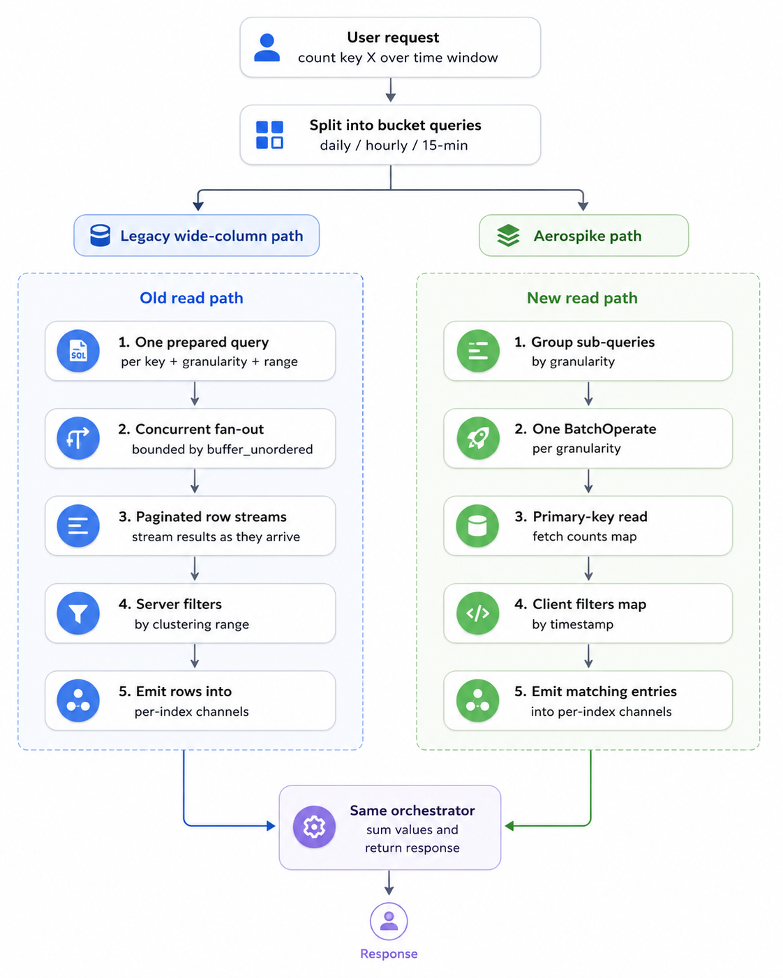
The two backends produce very different network shapes for the same logical query. The original backend returns many small paginated row streams, one per (key, granularity). The server filters by time range using the clustering column. Aerospike returns one batch response with the entire counts map per key, and the client filters the map to the requested range. The reader’s storage layer hides this difference: both paths emit (index, value, timestamp, granularity) tuples into the same per-index channels, and the orchestrator above sums them the same way.
The third approach performed best in testing. By collapsing many bucket records into a single record per counter, we reduced the total record count by more than an order of magnitude, which also reduced primary index memory. It also produced a smaller on-disk footprint, since the long counter key is stored once per record instead of being repeated across every bucket. The schema was chosen to fit the access pattern, with the index and disk savings following naturally.
The pipeline continues writing to the original backend as the primary, while Aerospike is added as a separate asynchronous shadow write behind a deterministic rollout logic. This lets us ramp Aerospike gradually and eventually cut over to it fully.
Reader: How each backend actually serves a query
The two storage backends sit behind the same execute_queries contract on the reader service, but what they do internally for a single batch read looks very different.
Figure 1. How a single read request flows through each backend.
The reader takes a batch of counter queries and decomposes each into one or more sub-queries per granularity (a 90-minute window for instance, becomes one hourly sub-query and two 15-minute sub-queries). In the original backend, each sub-query becomes its own prepared statement bound with (start_ms, end_ms, key), and the storage layer fires all of them concurrently as a stream of futures with buffer_unordered capping in-flight queries to a tuned bound. Each query returns a paginated row iterator, the server uses the clustering column to filter by time range and rows stream through to per-index channels as they arrive. So a single user request can produce many small queries, each a separate network round-trip to the partition master holding key, with results dribbled back over a paginated stream.
On Aerospike, the storage layer first groups all sub-queries by granularity, then issues one BatchOperate per granularity. Each sub-query becomes a single primary-key read against the appropriate set; the server returns the entire counts map for that key in one record. The client iterates the map and emits only the entries whose timestamps fall inside the requested range. This keeps the code simple, and at our map sizes the overhead is negligible. There’s no streaming, a batch read either succeeds or fails as a unit and there are at most three network round-trips per user request, one per granularity, regardless of how many sub-queries there are.
This reflects the different design philosophies of the two systems. Wide-column stores typically expect client-side fan-out for reads, while Aerospike’s batch API is designed for exactly this multi-key pattern.
A few issues with the Aerospike Rust client also surfaced during rollout, as it was less mature than its Go counterpart. For example, when we started, the officially available Rust client was synchronous, so every batch read had to be bridged through tokio::task::spawn_blocking with some amount of custom plumbing. Once the official async client was released, we removed that layer and saw measurable improvements in both p50 and p99 latency. The other issue was Domain Name System (DNS). The client resolved seed hostnames only during initialization and did not re-resolve them when the cluster topology refreshed. As a result, a full staging cluster replacement, with new IPs behind the same hostnames, left the client stuck on the old IPs until restart. We filed the bug upstream, and a fix shipped in a subsequent release. We also reproduced the scenario locally with a Docker-based end-to-end test and ran additional staging drills to confirm recovery before continuing the rollout.
Experiment with indexing
We run Aerospike in its default storage configuration, Hybrid Memory Architecture (HMA), where the primary index sits in Random-Access Memory (RAM) and the data sits on Solid-State Drive (SSD). The other relevant mode keeps both index and data in Dynamic Random-Access Memory (DRAM), which is more expensive and not something that fits our use-case. Even in HMA, the primary index grows linearly with record count. At our scale, that growth was a foreseeable issue.
To raise the memory ceiling, we tried moving the primary index itself from RAM to local Non-Volatile Memory Express (NVMe) while keeping data on SSD. We expected the extra index latency to be invisible within our overall request budget. In practice, we started seeing p99 spikes that did not track overall QPS. Instead, they followed I/O activity on hot keys. We observed that when many concurrent lookups land on the same record, the in-memory index handles them more prudently compared to a disk backed index. Adding more and better nodes improved things slightly but did not mitigate the issue. Consequently, we reverted back to in-memory index with a memory-optimized instance type.
Overall impact
The migration delivered gains across infrastructure, performance, and data footprint. Most of these improvements trace back to the schema redesign like collapsing rows into maps, rather than the database change itself.
The primary index currently uses about 50 GB of the roughly 100 GB usable memory per node. The same dataset is around 1 TB on disk, compared with around 3 TB on the original setup. This is primarily attributed to our adoption of the map-based schema discussed earlier.
In production, p99 read latency was consistently better than the original setup, with roughly 50% improvement across our read paths. The write path now uses a single atomic increment operation, replacing the read-modify-write pattern we had built previously.
The new setup costs roughly 45–50% less per node compared to our original setup. We also reduced the replication factor from 3 to 2, saving roughly a third of both storage and primary index memory. RF=2 can be awkward in databases that depend on write quorum, but Aerospike’s master-replica model still keeps an authoritative copy available after a single-node loss. That gives us meaningful fault tolerance even at RF=2. The remaining risk, a simultaneous multi-AZ failure, was acceptable for this workload because the writer continues producing increments from the source event stream. Any lost counter data can self-heal as new events arrive.
Conclusion
This migration ultimately came down to aligning the storage design with the workload. These results would not have been achieved by simply swapping one storage system for another. As the service evolved over time, our initial design choices became less optimal, and the migration surfaced opportunities to rethink them. The gains came from focusing on optimization opportunities, redesigning the data model, and cleanly separating storage concerns. Through shadow reads and writes, followed by a gradual rollout, we completed the migration with zero downtime and no data-integrity issues. The result is a system that fits its workload well and a foundation that makes future storage changes safer and easier to attempt.
Join us
Grab is Southeast Asia’s leading superapp, serving over 900 cities across eight countries (Cambodia, Indonesia, Malaysia, Myanmar, the Philippines, Singapore, Thailand, and Vietnam). Through a single platform, millions of users access mobility, delivery, and digital financial services, including ride-hailing, food delivery, payments, lending, and digital banking via GXS Bank and GXBank. Founded in 2012, Grab’s mission is to drive Southeast Asia forward by creating economic empowerment for everyone while delivering sustainable financial performance and positive social impact.
Powered by technology and driven by heart, our mission is to drive Southeast Asia forward by creating economic empowerment for everyone. If this mission speaks to you, join our team today!
AWS CloudFormation helps you model and provision cloud infrastructure as code using JSON or YAML templates, or through tools like the AWS Cloud Development Kit (CDK). Whether you create stacks directly, use change sets for preview, or deploy through CI/CD pipelines and AI agents, the speed of your deployment cycle directly impacts how fast you can iterate.
In March 2024, we published How we sped up AWS CloudFormation deployments with optimistic stabilization, where we explained how CloudFormation provisions resources and what happens during stabilization. That post introduced the CONFIGURATION_COMPLETE event and the optimistic stabilization strategy that reduced deployment times by up to 40%. Today, CloudFormation express mode takes this further.
Express mode is recommended for development workflows where you iterate frequently. It makes your deployments complete faster so you can get immediate feedback. For production deployments where you need resources ready to serve traffic before proceeding, the default behavior remains the right choice. Combined with pre-deployment validation, which catches template errors before provisioning begins, Express mode completes the iterate-faster picture: validate in seconds, deploy in seconds. To understand what express mode gives you, you first need to understand what CloudFormation has always done during deployment.
What CloudFormation does during deployment
When you add an AWS::SQS::Queue to your template and deploy, the queue is created. But can it receive messages yet? Often, no. There’s a window between “resource created” and “resource can serve traffic.” This is true across AWS services. An EC2 instance is “launched” before it can respond to HTTP requests. A CloudFront distribution is “created” before it propagates to edge locations worldwide. An ECS service is “active” before its containers pass health checks and reach desired capacity. And a Lambda function deletion isn’t complete until its network interfaces are cleaned up.
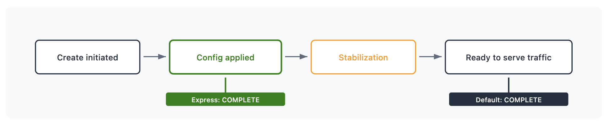
Figure 1: Single resource lifecycle phases
This process is called stabilization. Stabilization means that when a stack operation reports CREATE_COMPLETE, the resources can serve traffic. This is useful for production pipelines where “stack complete” should mean “ready to shift traffic.” Now, with express mode, you have a second option.
Express mode gives you control over when you want CloudFormation to report completion. With express mode, CloudFormation completes the stack operation as soon as resource configuration is applied. Resources continue becoming ready to serve traffic in the background. Regardless of mode, CloudFormation still:
Respects resource dependencies within the stack – if a resource references another resource’s ID or attribute, the referenced resource’s configuration is confirmed first. Resources with no dependencies on each other proceed in parallel.
Creates, updates, or deletes each resource the same way
Retries dependent resources that encounter transient failures during the operation
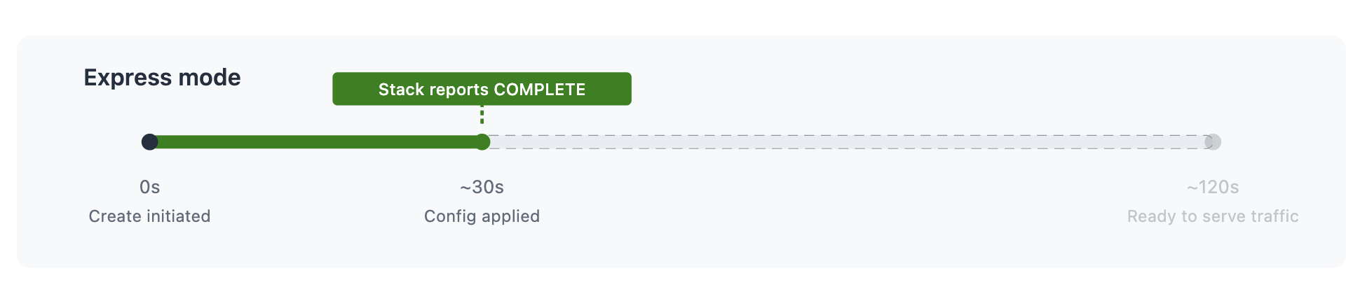
Here’s what that looks like for a deployment:
Figure 3: Express mode timeline
The resource takes the same time to become ready to serve traffic in both cases. Express mode makes your iteration cycle faster by not blocking you on the stabilization wait.
When this matters
Development iteration
You’re building a VPC with subnets, a security group, and an ALB. You need the ALB’s DNS name and the security group ID to configure the next layer of your application. You don’t need to send traffic to the ALB right now. You just need to know it exists and get its attributes. With Express mode, you get the ARN, the DNS name, and the security group bindings in seconds. You proceed to your next iteration.
AI agent workflows
An AI agent iterating on infrastructure needs a tight feedback loop: deploy, observe the result, adjust, deploy again. The agent doesn’t need the CloudFront distribution to propagate globally before deciding whether the template is correct. It needs confirmation that the configuration was accepted.
Express mode turns a 5-10 minute CloudFront deployment into a sub-minute confirmation. The agent can validate, refine, and redeploy multiple times in the window a single default deployment would have taken.
Dependent stack deployments
When you deploy multiple stacks in sequence, each stack operation completes faster with Express mode. Whether dependencies exist within a stack or across stacks via import/export, Express mode handles retries and waits to make sure dependent resources can still be provisioned. It moves faster without breaking your dependency chain
Getting started
Enable Express mode per operation with a single parameter:
Express mode disables rollback by default for faster iteration. If a resource fails to configure, the stack stays in place and you can fix and retry immediately. To re-enable rollback:
Use the --express flag with sam deploy or sam sync:
sam deploy --express

sam sync --express
To persist the setting, add --save-params and Express mode is saved to your samconfig.toml:
sam deploy --express --save-params
The --disable-rollback flag works alongside --express to control rollback behavior within the deployment configuration.
No template changes. No new resource types. The same template deploys the same resources. You’re choosing when to receive the “done” signal.
Additional considerations
Change sets: Express mode is supported with change sets. Specify --deployment-config at create-change-set time, and the configuration is stored with the change set and applied when executed.
Nested stacks: When you enable Express mode on a parent stack, it propagates to all nested stacks in the hierarchy. All resources across the hierarchy complete when configuration is applied.
Express mode gives you immediate confirmation that your infrastructure configuration is applied, so you can move to your next iteration without waiting for stabilization. It separates “is my configuration correct” from “are my resources serving traffic” and lets you decide which question you need answered right now.
For development iteration, AI agent workflows, and dependent stack deployments where you need resource identifiers rather than traffic readiness, Express mode delivers that answer much more quickly. For production deployments where “stack complete” should mean “ready to serve traffic,” the default behavior remains the right choice.
In August 2025, the CalyxOS privacy-focused
Android distribution announced
that it was pausing all releases while it reworked its
release process, security protocols, and changed its signing keys
following the departure of one of its founders. The project has now announced
that it is “officially back from the hiatus” with the
7.2.2.0 release.
CalyxOS 7.2.2.0 is signed by us using a new
HSM-based, open-source signing solution we designed to enhance the
security of the entire signing process, ensure redundancy, and remove
single points of failure. You can verify CalyxOS 7.2.2.0 and future
builds following these
instructions. For anyone who is interested, the security audit
report of the HSM provisioning ceremony script can be found here.
In addition, we also went through significant infrastructure
improvements. In particular, we have set up a cleaner server structure
to streamline each release. In response to Google’s less frequent AOSP
source code releases, our team developed scripts to reduce the
overhead in applying monthly patches and updates. Please keep in mind,
additional manual steps are still needed to compensate for AOSP
changes, such as requesting and storing kernel sources with each
update. Currently, our lead engineer is continuing the maintenance of
the base device trees for both LineageOS and CalyxOS to bridge the gap
created by the absence of Google Pixel device trees.
Managing high-volume application logs at scale presents challenges from slow query performance and difficulty running complex aggregations to maintaining real-time analytics on streaming data. Apache Iceberg materialized views with AWS Glue, Amazon Data Firehose, and AWS Lambda address these challenges by accelerating log analytics through pre-computed query results.
In this post, you learn how to build an application log pipeline for production use with Amazon CloudWatch Logs, AWS Lambda, Amazon Data Firehose, AWS Glue, and Apache Iceberg materialized tables. You then use materialized views to accelerate query performance. This solution helps you achieve faster query response times on large-scale log data without requiring you to manage continuous data lake refresh.
Solution overview
This solution accelerates log analytics by pre-computing query results through Apache Iceberg materialized views. By querying pre-aggregated results instead of scanning raw log data for every request, you can help reduce query response times. For example, queries that previously took minutes scanning terabytes of raw data may return in seconds from the compact materialized view. Results update automatically as new logs arrive, helping you handle high-volume log streams while maintaining fast analytics performance.
Architecture overview
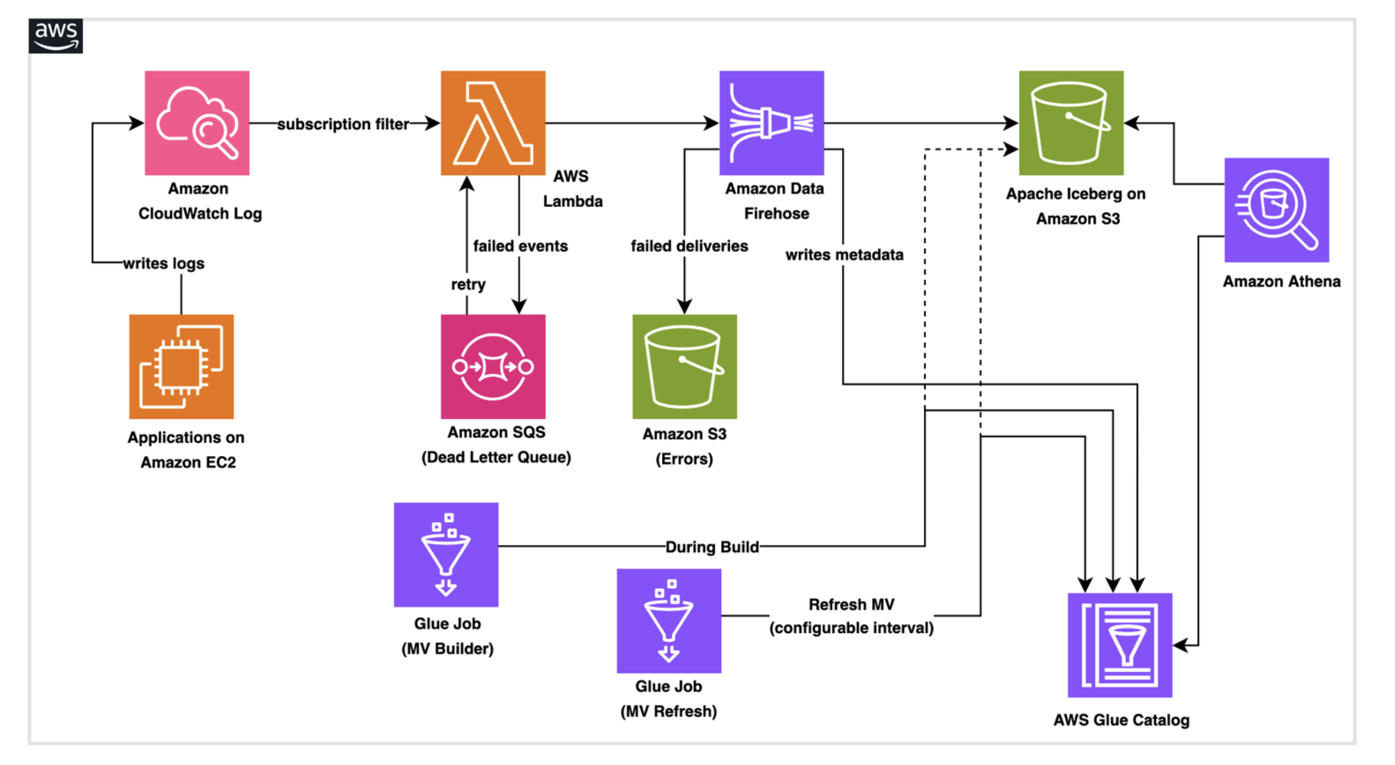
The architecture consists of AWS services working together to create a data pipeline:
Amazon CloudWatch Logs receives application logs and system events, then routes them to downstream targets using CloudWatch Logs subscription filters. CloudWatch Logs has a built-in retry mechanism. If the destination service returns a retryable error, CloudWatch Logs automatically retries delivery for up to 24 hours.
AWS Lambda serves as the transformation layer, parsing log messages, enriching data, and preparing records for storage.
Amazon Data Firehose buffers incoming data and handles the technical requirements of writing to Apache Iceberg tables (an open-source data table format), including batch optimization, schema validation, and automatic retry logic for failed writes.
AWS Glue runs a one-time job during stack creation to provision the Iceberg database, base table, and materialized view structure in the Data Catalog. A second scheduled Glue job refreshes the materialized view by recomputing aggregations from the base table on a configurable interval helping downstream queries through Amazon Athena return up-to-date, pre-aggregated results without scanning raw data.
This architecture is designed to support automatic scaling, serverless infrastructure, error handling that routes failed records to Amazon S3 for analysis and replay, capture of failed Lambda invocations for automatic retry, and real-time monitoring through Amazon CloudWatch metrics.
Prerequisites
Before you deploy the solution, review the following prerequisites.
AWS account with necessary permissions to execute an AWS CloudFormation template, run AWS Glue jobs, run queries to verify Iceberg table data using Amazon Athena.
Basic familiarity with Boto3 to understand Python code. Foundational understanding of Apache Iceberg concepts.
Solution deployment
The following deployment steps guide you through implementing this solution in your AWS account.
Step 1: Deploy the AWS CloudFormation pipeline stack
You can deploy this solution using an AWS CloudFormation stack. The template handles creating Amazon S3 buckets, uploading AWS Glue and Lambda scripts, provisioning IAM roles, configuring the Firehose delivery stream, and running the Glue job to create the Iceberg database, base table, and materialized view.
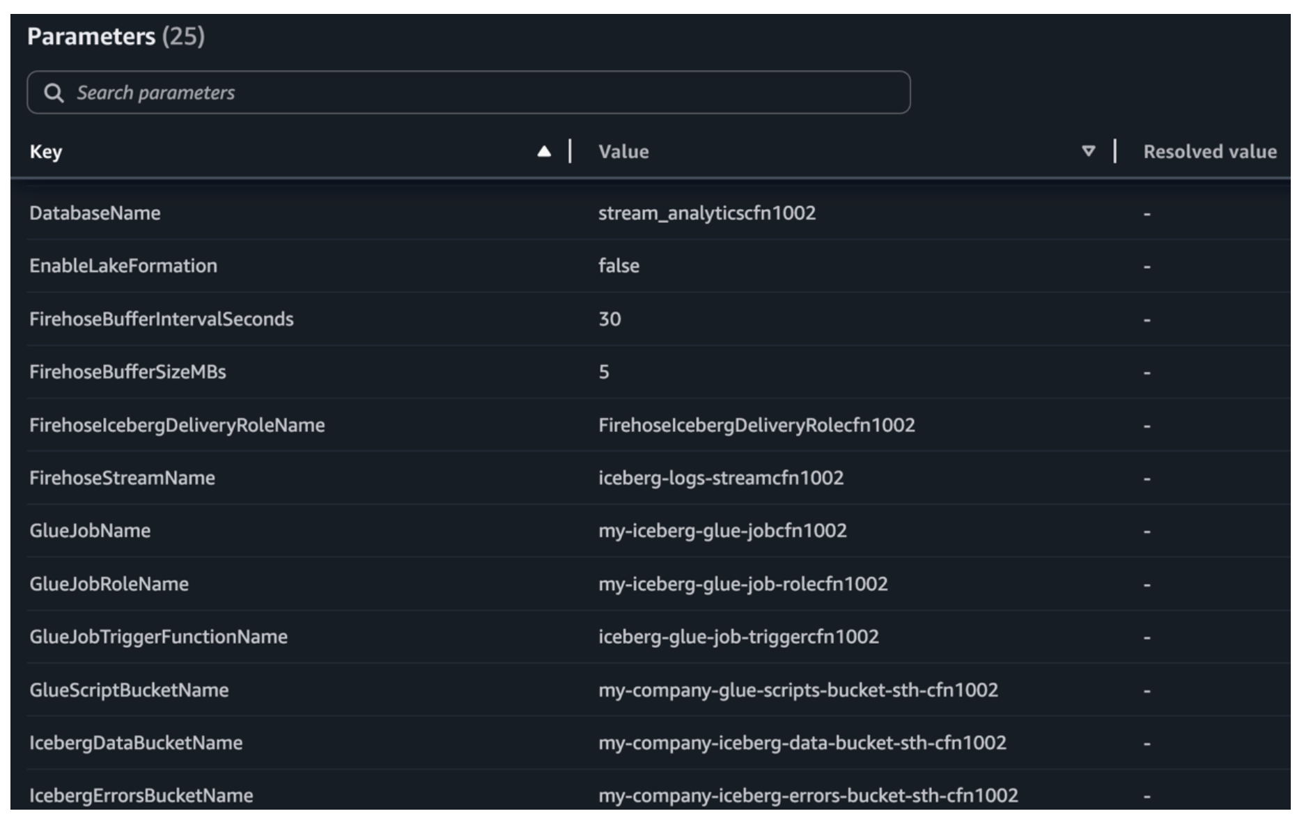
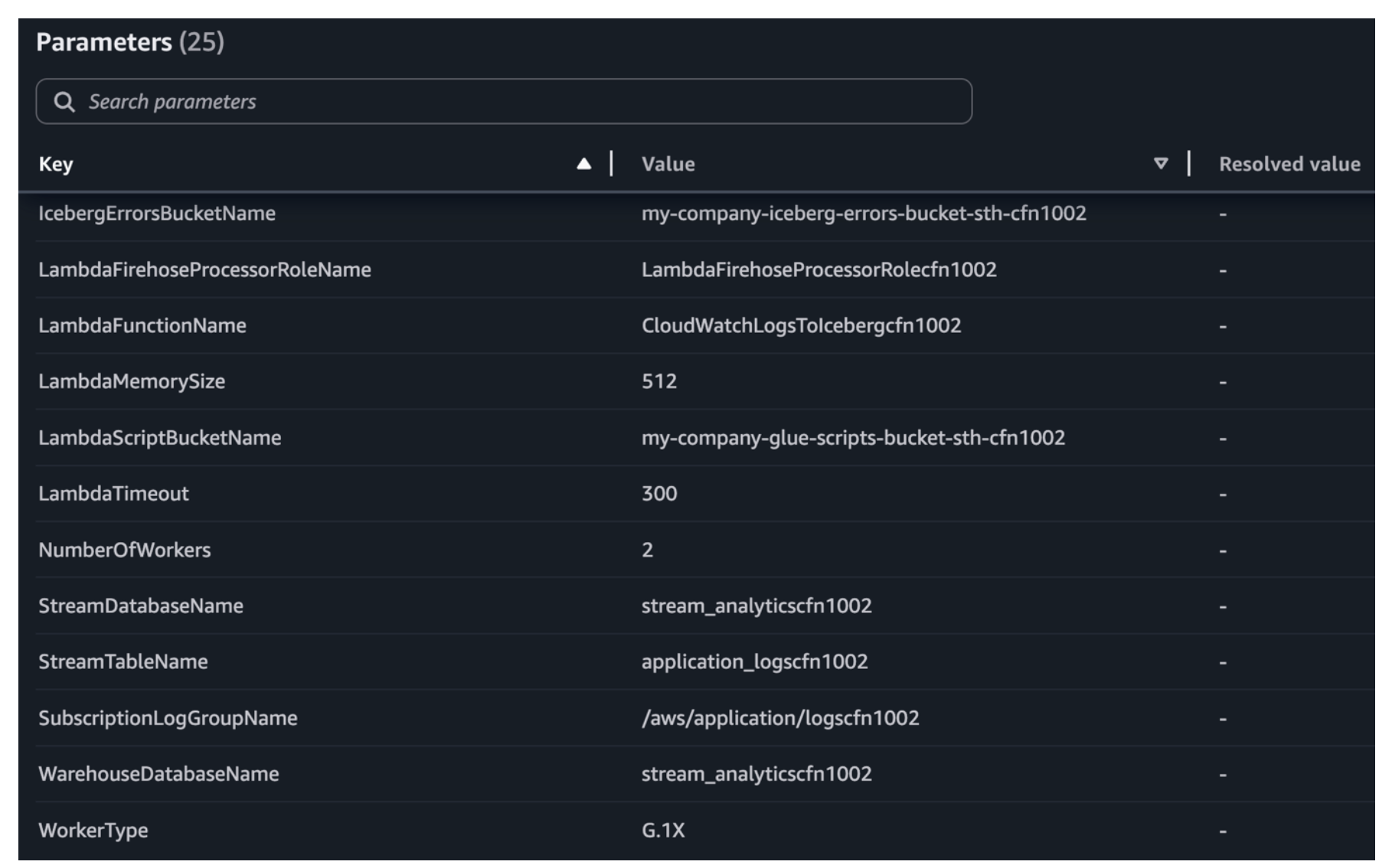
Launch the stack in the AWS CloudFormation console. Review the parameters marked REQUIRED and adjust the toggle options (CreateScriptBucket, EnableLakeFormation, CreateSubscriptionLogGroup) based on your environment. Other parameters include preconfigured defaults that you should review for your environment. Choose the CloudFormation stack to deploy resources using the AWS CloudFormation console.
Pipeline stack required parameters view in the AWS CloudFormation console.
Additional pipeline stack required parameters in the AWS CloudFormation console.
Step 2: Test the end-to-end pipeline
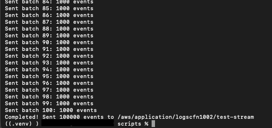
Send sample log events matching the Iceberg table schema (for example, id, customer_name, amount, and order_date) to the CloudWatch log group. The subscription filter triggers the Lambda, which forwards records to Firehose for delivery into the Iceberg table.
git clone https://github.com/aws-samples/sample-log-analytics-iceberg-mv.git
cd sample-log-analytics-iceberg-mv
python3 scripts/send_test_logs.py
Execution of test events.
Verify data delivery and refresh the materialized view
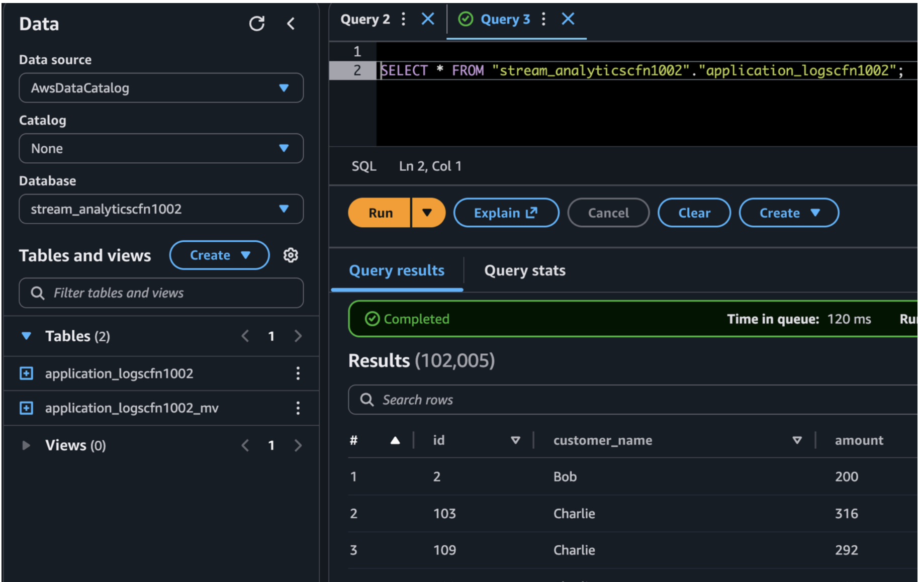
Allow approximately 30 seconds (learn more in Buffer data for dynamic partitioning) for the Firehose buffer to flush. After the buffer flushes, run the following query in Amazon Athena to verify that data has been successfully delivered to the base table.
Query result using Amazon Athena.
Automated materialized view refresh
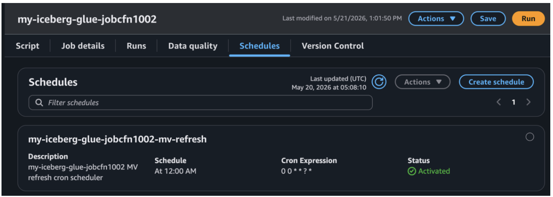
In this example, the AWS CloudFormation stack provisions a Glue job configured to run the materialized view (MV) refresh once daily at midnight UTC, meaning the MV reflects data up to the previous day. You can adjust the trigger’s cron schedule to match common MV refresh requirements such as hourly, every 15 minutes, or on demand.
The Glue job performs a full recomputation of the aggregations from the base Iceberg table and writes the results to the MV. Downstream consumers querying through Athena read from this pre-aggregated view, delivering faster performance. This is especially critical in real production scenarios where the base table contains millions of records and numerous columns. Computing aggregations directly from raw data at query time would degrade downstream application performance.
Job scheduled view in the AWS Glue console.
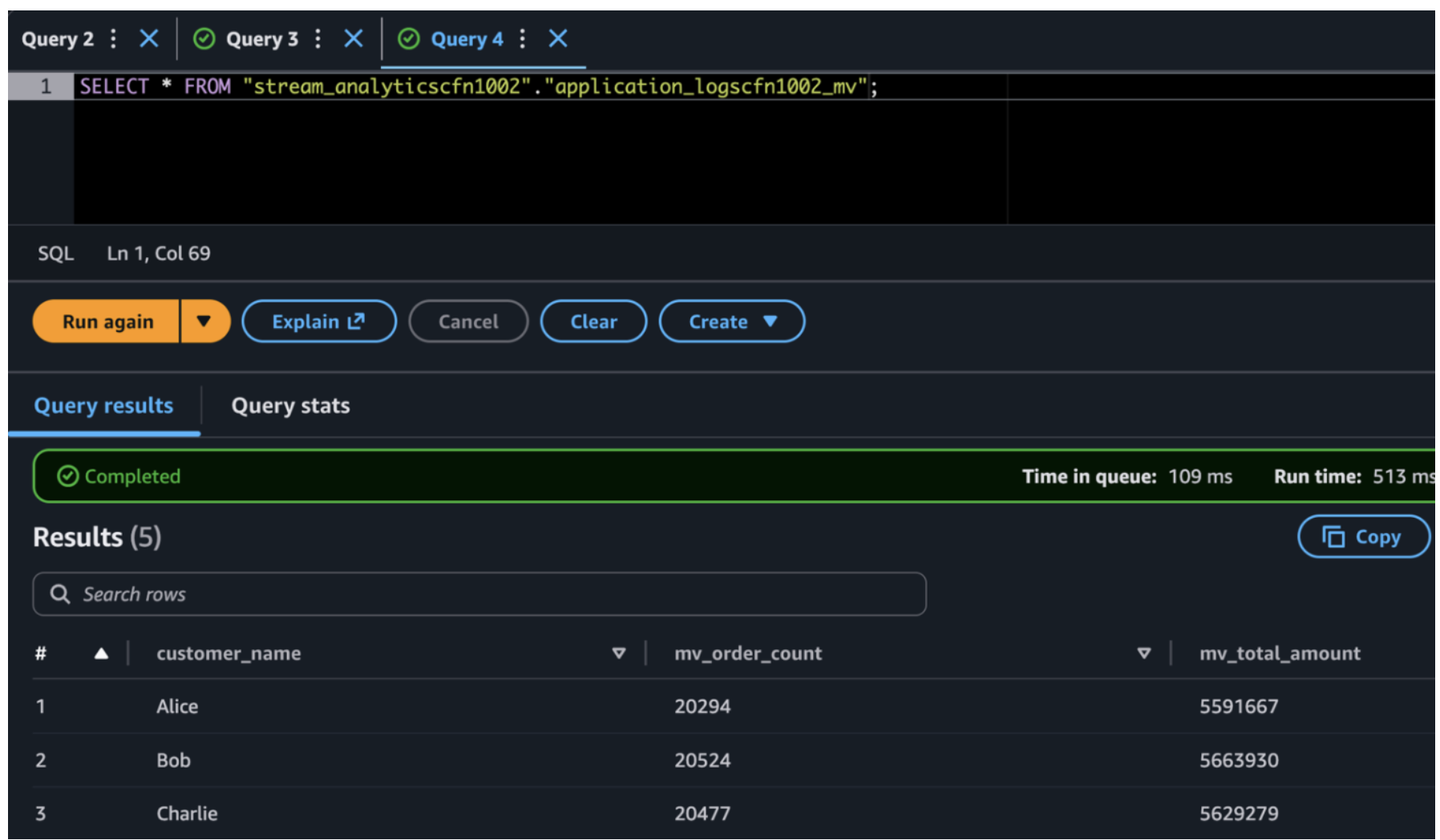
In a production environment, the base Iceberg table stores every individual order event, potentially millions of rows with dozens of columns growing daily. When dashboards or downstream applications need aggregated insights like daily revenue per customer or monthly order counts by region, querying the base table directly forces Athena to scan terabytes of raw data on every request. This results in slow response times and high costs at scale. The materialized view solves this by pre-computing these business-level aggregations once during the scheduled refresh, storing the results in a compact, purpose-built table with far fewer rows and columns. This means a dashboard query that would scan millions of raw records now reads from a pre-aggregated table, designed to reduce query response time. The base table remains your source of truth for granular, row-level lookups, while the materialized view serves as the performance layer for repeated analytical queries with embedded business logic.
Materialized View query result using Amazon Athena
Alternative: Amazon S3 Tables
This solution can also be implemented using Amazon S3 Tables, which provides a fully managed Apache Iceberg experience with native support for materialized views. In this post, we use the Glue-based approach to demonstrate the underlying mechanics and provide full flexibility to customize refresh logic for your specific requirements. To learn more, see Getting started with S3 Tables.
Clean up
To avoid incurring future charges, delete the resources you created as part of this exercise if you are not planning to use them further. Delete the stacks created in the previous steps, then empty and delete the Amazon S3 buckets.
Conclusion
This solution shows how to build a scalable application log data pipeline that delivers log events from Amazon CloudWatch Logs to Apache Iceberg tables using AWS Lambda and Amazon Data Firehose. This architecture uses fully managed AWS services to minimize operational overhead while providing high availability and consistent performance.
Key strengths include serverless infrastructure designed to support automatic scaling, error handling designed to route failed records to Amazon S3 for troubleshooting and replay, and analytics capabilities through Apache Iceberg’s ACID transactions and query performance optimizations. As you move this solution into production, we recommend that you implement data quality checks in Lambda and configure encryption at rest and in transit for your data. You can also establish data retention policies and explore partitioning strategies for better query performance.
You now have a log analytics pipeline built for production use that scales with your workload.
A few astute observers have noticed that some
content on kernel.org had disappeared and were understandably
concerned. Konstantin Ryabitsev has provided an update via
social.kernel.org:
There was an unfortunate error while changing the kernel.org
primary/secondary mirroring infrastructure, which resulted in the /pub
tree suddenly becoming empty. No data was lost, just public mirror
copies. Everything is now being restored, but deletes are fast and
restores are slow, so thank you for your patience!
The incident is
being tracked on the Linux Foundation’s IT status page.
Building and maintaining clusters for data processing with Apache Spark has long been a pain point for organizations of all sizes. Traditional deployments require significant operational overhead and present multiple challenges that slow down time-to-insight and increase total cost of ownership. In this post, we will demonstrate three integration patterns that let data teams focus on analytics instead of infrastructure management.
Consider the typical experience of data teams working with self-managed Spark clusters:
Infrastructure complexity – Teams must manage Amazon Elastic Compute Cloud (Amazon EC2) instances, networking, security groups, and cluster configurations across development, staging, and production environments.
Cost unpredictability – Idle clusters continue consuming resources and generating bills, while automatic scaling policies often lag behind actual demand patterns.
Operational burden – DevOps teams spend significant time patching, monitoring, and troubleshooting cluster health issues.
Development friction – Data scientists and engineers must wait for cluster provisioning before they can begin exploratory analysis, slowing down iterative development cycles.
Interactive workload challenges – Managing interactive Spark workloads typically requires additional components, exposing specific ports, and complex network configurations.
These challenges become especially pronounced when organizations need to support multiple concurrent workloads: notebooks for data scientists, scheduled pipelines for data engineers, and ad hoc queries for analysts. The traditional approach encourages teams to choose between maintaining multiple clusters (expensive) or sharing resources (contentious) while maintaining fixed endpoint connectivity for interactive workloads (usually exposing JDBC ports for the Thrift protocol).
The Apache Spark engine in Amazon Athena addresses these operational challenges by providing a fully managed, serverless Spark execution environment. Built on Firecracker micro-VMs (AWS’s lightweight virtualization technology) and running the AWS-optimized Spark 3.5.6 engine with Spark Connect support, Athena with Apache Spark launches and scales in seconds, reducing costs for unpredictable workloads and infrastructure operational overhead.
Athena with Apache Spark is already integrated as a compute engine within Amazon SageMaker Unified Studio notebooks, providing rapid startup and scaling, making it ideal for ad hoc data exploration and transformations.
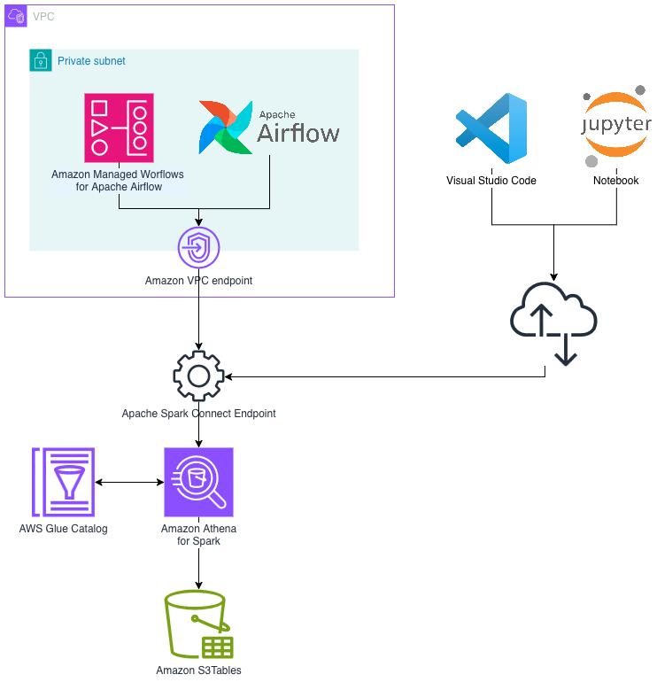
This post shows how developers, data engineers, and analysts can connect to a secure Spark Connect endpoint in Athena with Apache Spark. You can use your preferred tools, such as Jupyter notebooks, VS Code, or dbt with Apache Airflow, without managing cluster lifecycle or scaling.
Solution overview
We explore three integration patterns that demonstrate how the flexibility of Athena with Apache Spark can reduce operational overhead and accelerate innovation with on-demand resource readiness:
Pattern A: Interactive analysis with Jupyter notebooks – Data scientists connect notebooks directly to Athena with Apache Spark for exploratory analysis and feature engineering.
Pattern B: Local development with VS Code – Software engineers develop Spark applications in their preferred IDE (integrated development environment) while executing on serverless compute.
Pattern C: Scheduled pipelines with dbt + Apache Airflow – Data engineers run production transformation pipelines with proper orchestration and session lifecycle management.
The following diagram illustrates the high-level architecture for connecting to Athena with Apache Spark using Spark Connect.
What’s new in the Apache Spark engine in Amazon Athena
In November 2025, the Apache Spark engine in Amazon Athena released a significant update with rapid session creation times and capabilities that weren’t possible with previous iterations:
Secure Spark Connect – Adds Spark Connect as a fully managed, authenticated, and authorized AWS endpoint for remote connectivity from Spark-compatible tools. For more information, see Spark Connect support.
Session-level cost attribution – Track costs per interactive session in AWS Cost Explorer or Cost and Usage Reports for granular chargeback and budgeting. For more information, see Session level cost attribution.
Advanced debugging capabilities – Live Spark UI and Spark History Server support for debugging workloads from both APIs and notebooks. For more information, see Accessing the Spark UI.
An Athena with Apache Spark workgroup configured with the latest Spark 3.5.6 engine.
Python 3.9+ installed locally.
AWS credentials configured.
Note: This tutorial creates AWS resources that incur charges, including Athena sessions (charged per DPU-hour), Amazon S3 storage, and data transfer. Athena sessions are charged while active, even if idle within the timeout period. Follow the cleanup instructions at the end of this post to avoid ongoing charges.
Provisioning workflow overview
The workflow for using the Apache Spark engine in Amazon Athena with Spark Connect follows these steps:
Create the session – Use the AWS API (start_session) to initialize a Spark session. The Spark driver is immediately ready to process requests (no JVM startup time).
Get the Spark Connect endpoint – Retrieve the endpoint URL and authentication token using get_session_endpoint.
Configure Your Tools – Set the SPARK_REMOTE environment variable or configure your tool with the Spark Connect URL.
Run Processing Steps – Run your Spark code as you normally would, but in a fully serverless environment that scales automatically based on your needs.
Monitor via Spark UI – Access the live Spark UI for debugging and performance monitoring using get_resource_dashboard.
Terminate the session – Clean up resources when finished using terminate_session.
By default, the session is configured with autoscaling using Spark Dynamic Resource Allocation up to 60 workers and an idle timeout of 20 minutes. You can change the default configuration at the workgroup level when creating it (create_work_group API) or when creating the session (start_session API).
Pattern A: Interactive analysis with Jupyter notebooks
The Jupyter notebook integration provides an interactive environment for exploratory data analysis, feature engineering, and model preparation. Notebooks connect directly to Athena with Apache Spark sessions for rapid iteration without cluster management.
Set up the environment
Create and activate a Python virtual environment, then install the required dependencies and start JupyterLab:
Before connecting, create an Athena with Apache Spark workgroup on the AWS Management Console:
Navigate to Amazon Athena → Workgroups → Create workgroup.
Select Apache Spark as the analytics engine.
Choose the Spark 3.5.6 engine version.
Configure the IAM role for the workgroup.
Configure the Amazon S3 output location.
Note: If you used Athena with Apache Spark previously, you need to create a new workgroup to use the latest version with Spark Connect support.
Create a session and connect
In your Jupyter notebook, use boto3 to create a session and establish the Spark Connect connection:
import boto3

# Initialize the Athena client
client = boto3.client('athena', region_name='us-east-1') # Replace with your region

# Start a new Spark session
response=client.start_session(
    WorkGroup='your-workgroup-name',
    EngineConfiguration={}
)
session_id=response['SessionId']
print(f"Session created: {session_id}")

# Get the session endpoint and authentication token
response=client.get_session_endpoint(SessionId=session_id)
authtoken=response['AuthToken']
endpoint_url=response['EndpointUrl']

# Build the Spark Connect URL
endpoint_url=endpoint_url.replace("https", "sc") + ":443/;use_ssl=true;"
url_with_headers=f"{endpoint_url}x-aws-proxy-auth={authtoken}"

# Create the Spark session
from pyspark.sql import SparkSession
from pyspark.sql.functions import col, rand, sum, avg, count

spark = SparkSession.builder \
    .remote(url_with_headers) \
    .getOrCreate()

# Verify the connection
spark.sql("SELECT 1").show()
Run queries and observe automatic scaling
Generate a larger dataset to trigger executor scaling. You can monitor the scaling behavior through the Spark UI:
# Generate large dataset to trigger executor scaling
large_data = spark.range(0, 10000000, numPartitions=100)

# Heavy computation that will require more executors
result=large_data.select(
    col("id"),
    (col("id") * col("id")).alias("squared"),
    rand().alias("random")
).groupBy((col("id") % 1000).alias("group")).agg(
    sum("squared").alias("sum_squared"),
    avg("random").alias("avg_random"),
    count("*").alias("count")
).orderBy("group")

result.show()
Access the Spark UI
Each session comes with a secure URL serving the Spark UI, to monitor and debug applications:
import os

# Get account ID
sts=boto3.client("sts")
account_id=sts.get_caller_identity()["Account"]

# Build session ARN
partition=os.environ.get("AWS_PARTITION", "aws")
region="us-east-1"
workgroup="your-workgroup-name"
session_arn=f"arn:{partition}:athena:{region}:{account_id}:workgroup/{workgroup}/session/{session_id}"

# Get Spark UI URL
ui_response=client.get_resource_dashboard(ResourceARN=session_arn)
print(f"Spark UI: {ui_response['Url']}")
Pattern B: Local development with VS Code
VS Code integration lets you develop Spark applications locally in your preferred IDE while executing on Amazon Athena with Apache Spark compute. This pattern is ideal for building reusable libraries, testing transformations, and developing production-ready code.
Set up the environment
Create a virtual environment and install dependencies:
The workflow is identical to Pattern A. You start a session with boto3, build the Spark Connect URL, and create a SparkSession. The key difference is setting the SPARK_REMOTE environment variable, which allows SparkSession.builder.getOrCreate() to connect automatically:
import os
import boto3

# Start session and get endpoint (same as Pattern A)
client=boto3.client('athena', region_name='us-east-1')
response=client.start_session(WorkGroup='your-workgroup', EngineConfiguration={})
session_id=response['SessionId']
response=client.get_session_endpoint(SessionId=session_id)
endpoint_url=response['EndpointUrl'].replace("https", "sc") + ":443/;use_ssl=true;"
spark_remote=f"{endpoint_url}x-aws-proxy-auth={response['AuthToken']}"

# Set environment variable for automatic connection
os.environ["SPARK_REMOTE"]=spark_remote

# Now SparkSession connects automatically
from pyspark.sql import SparkSession
spark=SparkSession.builder.getOrCreate()
Note: The SPARK_REMOTE URL contains a short-lived authentication token that expires with the session. For production workloads, retrieve the token on demand using get_session_endpoint() rather than storing it persistently. Avoid logging or persisting this value.
This same pattern works with most Spark-compatible development environments. AI coding assistants like Claude Code, Cursor, and Kiro benefit particularly well from this approach. The ability to spin up a fresh Athena with Apache Spark session in seconds means developers can rapidly iterate on generated code and test transformations immediately. They can tear down sessions when done, without maintaining a persistent cluster between coding sessions.
Pattern C: Scheduled pipelines with dbt + Airflow
For production data pipelines, combining dbt (data build tool) with Apache Airflow orchestration provides a robust, version-controlled approach to managing complex transformation workflows. Athena with Apache Spark executes the dbt models with serverless compute, eliminating cluster management overhead.
Install dependencies
The key dependencies for dbt with Athena with Apache Spark must be installed in the correct order:
pip install pyspark[connect]==3.5.6 # Install first to ensure correct version
pip install dbt-spark[session]
pip install setuptools
Important: Install pyspark[connect]==3.5.6 first to make sure dbt uses the compatible PySpark version.
Configure dbt profile
Configure dbt to use Spark Connect with a session-based connection. Create a profiles.yml file:
The method: session configuration uses a local Spark session. When pyspark[connect]==3.5.6 is installed and the SPARK_REMOTE environment variable is set, dbt automatically connects through Spark Connect.
spark_connect_profile:
  target: dev
  outputs:
    dev:
      type: spark
      method: session
      schema: default
      database: default
      host: NA # Ignored by method=session
      user: dummy # Placeholder
      connect_timeout: 30
      connect_retries: 0
Create a dbt model
Create a dbt model that writes to Apache Iceberg format (models/bucketed_data.sql):
{{ config(
    materialized='table',
    file_format='iceberg',
    catalog='iceberg',
    location_root='s3://your-bucket/iceberg-tables'
) }}

WITH numbers AS (
    SELECT id
    FROM range(0, 100000)
),
buckets AS (
    SELECT
        id,
        id % 10 AS bucket,
        current_timestamp() AS created_at
    FROM numbers
)
SELECT * FROM buckets
setup_athena_session – A PythonOperator that starts the session and pushes spark_remote_url to XCom.
run_dbt – A BashOperator that sets SPARK_REMOTE from XCom and runs dbt.
terminate_athena_session – A PythonOperator with trigger_rule=ALL_DONE to make sure cleanup runs even on failure.
from airflow import DAG
from airflow.operators.python import PythonOperator
from airflow.operators.bash import BashOperator
from airflow.utils.trigger_rule import TriggerRule
from datetime import datetime

with DAG(
    dag_id="athena_dbt_pipeline",
    schedule="@daily",
    catchup=False,
    start_date=datetime(2025, 1, 1),
) as dag:

    setup_session=PythonOperator(
        task_id="setup_athena_session",
        python_callable=setup_athena_session, # similar boto3 flow demonstrated earlier
    )

    run_dbt=BashOperator(
        task_id="run_dbt",
        bash_command="""
        export SPARK_REMOTE="{{ (ti.xcom_pull(task_ids='setup_athena_session') or {}).get('spark_remote_url', '') }}"
        source /path/to/dbt-env/bin/activate
        dbt run --project-dir . --profiles-dir .
        """
    )

    close_session=PythonOperator(
        task_id="terminate_athena_session",
        python_callable=terminate_athena_session,
        trigger_rule=TriggerRule.ALL_DONE,
    )

    setup_session >> run_dbt >> close_session
Security and best practices
When you connect to Athena with Apache Spark, follow these practices to protect your data and credentials.
Spark Connect security
Athena with Apache Spark uses Spark Connect to securely transmit queries and receive results. All communication is encrypted end-to-end using TLS 1.2+. Session tokens are short-lived and automatically rotated.
Recommendations:
Use IAM roles for authentication rather than long-lived credentials.
Session tokens have a limited lifetime, so refresh them for long-running operations.
Monitor Spark Connect activity in AWS CloudTrail for audit compliance.
IAM permissions
Implement least-privilege IAM policies. At minimum, the following permissions are required:
athena:StartSession, athena:TerminateSession, athena:GetSession, athena:GetSessionEndpoint, and athena:GetResourceDashboard on your workgroup.
Amazon S3 permissions for your data buckets.
AWS Glue Data Catalog permissions for your database and table access.
Clean up
To avoid ongoing charges, remove the resources created during this walkthrough:
Delete the Athena workgroup you created for this tutorial using the Amazon Athena console or the DeleteWorkGroup API.
Remove Amazon S3 objects created during testing, including query results and Iceberg table data at your configured output location. Data written to Amazon S3 persists after session termination and continues to incur storage costs.
Delete any IAM roles created specifically for this walkthrough.
Remove any AWS Glue Data Catalog databases and tables created during testing.
Conclusion
The Apache Spark engine in Amazon Athena with Spark Connect support transforms how teams build and operate Spark workloads. By eliminating cluster management overhead and providing near-instant, serverless compute, data teams can focus on delivering insights rather than managing infrastructure.
The three patterns covered in this post demonstrate the flexibility of Athena with Apache Spark:
Pattern A (Jupyter notebooks) – Ideal for data scientists doing exploratory analysis and feature engineering.
Pattern B (VS Code) – Well-suited for software engineers building production-ready Spark applications.
Pattern C (dbt + Airflow) – Well-suited for data engineers running scheduled, version-controlled transformation pipelines.
With rapid session creation, automatic scaling, and pay-per-use pricing, Athena with Apache Spark provides a compelling alternative to self-managed Spark clusters.
To provide the best experiences, we use technologies like cookies to store and/or access device information. Consenting to these technologies will allow us to process data such as browsing behavior or unique IDs on this site. Not consenting or withdrawing consent, may adversely affect certain features and functions.
Functional
Always active
The technical storage or access is strictly necessary for the legitimate purpose of enabling the use of a specific service explicitly requested by the subscriber or user, or for the sole purpose of carrying out the transmission of a communication over an electronic communications network.
Preferences
The technical storage or access is necessary for the legitimate purpose of storing preferences that are not requested by the subscriber or user.
Statistics
The technical storage or access that is used exclusively for statistical purposes.The technical storage or access that is used exclusively for anonymous statistical purposes. Without a subpoena, voluntary compliance on the part of your Internet Service Provider, or additional records from a third party, information stored or retrieved for this purpose alone cannot usually be used to identify you.
Marketing
The technical storage or access is required to create user profiles to send advertising, or to track the user on a website or across several websites for similar marketing purposes.