Седмицата (5–10 май)

Post Syndicated from Светла Енчева original https://www.toest.bg/siedmitsata-5-10-may/

Седмицата (5–10 май)

Католическият свят си има нов папа – Лъв XIV. И всички се радват. Тръмпистите – че той е американец, един вид, техен човек. Останалите – че макар и американец, доскорошният кардинал Робърт Превост никак не прилича на Тръмп, а възгледите му го сродяват по-скоро с предшественика му – папа Франциск.

И докато във Ватикана се показва дим само при избора на нов предводител на Католическата църква, в България димките за отвличане на вниманието са обичайна практика. Една от актуалните е заявката на МОН, че няма всички ученици задължително да учат православие, а ще могат да избират между него, ислям и светски добродетели.

На практика обаче, за да се изучава един задължителноизбираем предмет, за него трябва да се съберат повече от 10 ученици. Силно вероятно е върху училищата да се упражнява натиск да се предлага приоритетно православието – и защото такава е политическата воля, и защото повечето учители членуват в синдиката на Янка Такева, която много държи на задължителното въвеждане на религията в училище. И родителите ще са карани да подписват, че искат религия, с аргументи като например, че няма достатъчно учители, за да се предлагат алтернативни варианти.

Чудя се обаче: ако в един клас има 20 мюсюлманчета и 2 православни християнчета, християнчетата ислям ли ще трябва да учат? Или не е политкоректно да си задавам такива въпроси?

За политкоректността по български е и новата статия на Александър Драганов. Той повдига въпроса за привилегиите в България, които свързва с бившата социалистическа номенклатура – със зъби и нокти тя се опитва да се консервира, тоест да запази позициите си и да облагодетелства наследниците си. Александър смята, че този проблем трябва да се реши, преди да стигнем до въпросите за расата и пола.

Проблемите с расата и пола в България обаче не стоят на пауза, докато останките от номенклатурата не се изпарят в небитието на някое хипотетично бъдеще. Затова в „Тоест“ ги държим под око. След събарянето на къщите в „Захарна фабрика“ и оставянето на около 200 души на улицата обръщаме специално внимание на ромските гета и тази седмица имаме две публикации по темата.

„Изоставеното наследство. Защо България не може да продължи да пренебрегва правото на дом“ е статията на Сара Перин, изпълнителна директорка на „Тръст за социална алтернатива“. Тя анализира историческия генезис на сегрегацията на ромите още от 50-те години на XX в. и дава предложения за адекватна жилищна политика, която не дискриминира и не създава бездомници.

Ина Иванова пък разговаря с живеещия във Франция Абдулсамед Вели, който е главен редактор на „Филибелии“ – онлайн медията на пловдивския квартал „Столипиново“. Може би и вие като мен тепърва научавате, че има такъв уебсайт. А него не само го има, ами е достъпен на цели осем езика – български, английски, френски, немски, италиански, руски, испански и турски. Не се сещам за друга българска онлайн медия, която може да се похвали с такова нещо.

Междувременно на първия тур на президентските избори в съседна Румъния пропутинският кандидат Джордже Симион излезе начело с убедителна преднина. Емилия Милчева разсъждава по темата какво ще стане, ако български Симион се яви на бял кон на президентските избори догодина. Докато националната ни сигурност се занимава с частни поръчки, няма причина това да не се случи.

Или чакайте – ние български Симион нямаме ли си вече? Или по-скоро Симион е румънски Радев? Ами ето – българският президент реши да отбележи Деня на Европа, като… инициира референдум срещу еврото. Подходящо, а?

Но да си проветрим душите с малко култура. В рубриката „На второ четене“ Стефан Иванов ни припомня три книги на български автори – „Дървета за прегръщане“ от Цветелина Александрова, „Това е краят на света и се чувствам добре“ от Стефан Касев и „Инструкции за направа на тигър“ от Георги Анев. Не бих могла да резюмирам статията на Стефан по-добре от самия него:

„Три начина да се сглоби фигурата на отчуждения, влюбен, вътрешно разкъсан човек. Александрова пише, сякаш гледа през прозореца с мокра чаша в ръка. Касев пише с кал по обувките и с вътрешен глас, който се пита: „Защо?“ Анев по-скоро реже месо от съвременността с хирургическа насмешка.“

Като стана дума за хирургическа насмешка, веднага се сещам за Елена Телбис. „Ние отдавна сме хвърлени в бездната, следователно не можем да бъдем хвърлени някъде, където вече сме“, казва тя в епизод 13 на „Т.Е. от Е.Т.“:

Дойде време за препоръката ми. Този път тя е за изложба.

Мартин Атанасов е много интересен визуален артист, който умее да пресъздава смисъл чрез детайли от изображения. Такава е и новата му изложба, която може да срещнете под имената „Чупливи очертания“ или „Крехки очертания“ (Fragile Outlines на английски). В нея той изследва телата на куиър хората, които се чувстват не на място в света, защото той сякаш не е предназначен за тях.

Изложбата е в галерия „Октопод“ в подлеза на „Сердика“. В нея се влиза през една малка врата при изхода към бул. „Дондуков“, която е много лесно да не се забележи.

Приятно четене и гледане! А ние сме горди, че съществуваме благодарение на вашата подкрепа.

Behind the Scenes: Building a Robust Ads Event Processing Pipeline

Post Syndicated from Netflix Technology Blog original https://netflixtechblog.com/behind-the-scenes-building-a-robust-ads-event-processing-pipeline-e4e86caf9249

Kinesh Satiya

Introduction

In a digital advertising platform, a robust feedback system is essential for the lifecycle and success of an ad campaign. This system comprises of diverse sub-systems designed to monitor, measure, and optimize ad campaigns. At Netflix, we embarked on a journey to build a robust event processing platform that not only meets the current demands but also scales for future needs. This blog post delves into the architectural evolution and technical decisions that underpin our Ads event processing pipeline.

Ad serving acts like the “brain” — making decisions, optimizing delivery and ensuring right Ad is shown to the right member at the right time. Meanwhile, ad events, after an Ad is rendered, function like “heartbeats”, continuously providing real-time feedback (oxygen/nutrients) that fuels better decision-making, optimizations, reporting, measurement, and billing. Expanding on this analogy:

  • Just as the brain relies on continuous blood flow, ad serving depends on a steady stream of ad events to adjust next ad serving decision, frequency capping, pacing, and personalization.
  • If the nervous system stops sending signals (ad events stop flowing), the brain (ad serving) lacks critical insights and starts making poor decisions or even fails.
  • The healthier and more accurate the event stream (just like strong heart function), the better the ad serving system can adapt, optimize, and drive business outcomes.

Let’s dive into the journey of building this pipeline.

The Pilot

In November 2022, we launched a brand new basic ads plan, in partnership with Microsoft. The software systems extended the existing Netflix playback systems to play ads. Initially, the system was designed to be simple, secure, and efficient, with an underlying ethos of device-originated and server-proxied operations. The system consisted of three main components: the Microsoft Ad Server, Netflix Ads Manager, and Ad Event Handler. Each ad served required tracking to ensure the feedback loop functioned effectively, providing the external ad server with insights on impressions, frequency capping (advertiser policy that limits the number of times a user sees a specific ad), and monetization processes.

Key features of this system include:

  1. Client Request: Client devices request for ads during an ad break from Netflix playback systems, which is then decorated with information by ads manager to request ads from the ad server.
  2. Server-Side Ad Insertion: The Ad Server sends ad responses using the VAST (Video Ad Serving Template) format.
  3. Netflix Ads Manager: This service parses VAST documents, extracts tracking event information, and creates a simplified response structure for Netflix playback systems and client devices.
     — The tracking information is packed into a structured protobuf data model.
     — This structure is encrypted to create an opaque token.
     — The final response, informs the client devices, when to send an event and the corresponding token.
  4. Client Device: During ad playback, client devices send events accompanied by a token. The Netflix telemetry system then enqueues all these events in Kafka for asynchronous processing.
  5. Ads Event Handler: This component is a Kafka consumer, that reads/decrypts the event payload and forwards the tracking information encoded back to the ad server and other vendors.
Fig 1: Basic Ad Event Handling System

There is an excellent prior blog post that explains how this systems was tested end-to-end at scale. This system design allowed us to quickly add new integrations for verification with vendors like DV, IAS and Nielsen for measurement.

The Expansion

As we continued to expand our third-party (3P) advertising vendors for measurement, tracking and verification, we identified a critical trend: growth in the volume of data encapsulated within opaque tokens. These tokens, which are cached on client devices, present a risk of elevated memory usage, potentially impacting device performance. We also anticipated increase in third-party tracking URLs, metadata needs, and more event types as our business added new capabilities.

To strategically address these challenges, we introduced a new persistence layer using Key-Value abstraction, between ad serving and event handling system: Ads Metadata Registry. This transient storage service stores metadata for each Ad served, and upon callback, event handler would read the tracking information to relay information to the vendors. The contract between the client device and Ads systems continues to use the opaque token per event, but now, instead of tracking information, it contains reference identifiers — Ad ID, the corresponding metadata record ID in the registry and the event name. This approach future proofed our systems to handle any growth in data that needs to pass from ad serving to event handling systems.

Fig 2: Storage service between Ad Serving & Reporting

The Evolution

In January of 2024, we decided to invest in in-house advertising technology platform. This implied that the event processing pipeline had to evolve significantly — attain parity with existing offerings and continue to support new product launches with rapid iterations using in-house Netflix Ad Server. This required re-evaluation of the entire architecture across all of Ads engineering teams.

First, we made an inventory of the use-cases that would need to be supported through ad events.

  1. We’d need to start supporting frequency capping in-house for all ads through Netflix Ad server.
  2. Incorporate pricing information for impressions to set the stage for billing events, which are used to charge advertisers.
  3. A robust reporting system to share campaign reports with advertisers, combined with metrics data collection, helps assess the delivery and effectiveness of the campaign.
  4. Scale event handler to perform tracking information look-ups across different vendors.

Next, we examined upcoming launches, such as Pause/Display ads, to gain deeper insights into our strategic initiatives. We recognized that Display Ads would utilize a distinct logging framework, suggesting that different upstream pipelines might deliver ad telemetry. However, the downstream use-cases were expected to remain largely consistent. Additionally, by reviewing the goals of our telemetry teams, we saw large initiatives aimed at upgrading the platform, indicating potential future migrations.

Keeping the above insights & challenges in mind,

  • We planned a centralized ad event collection system. This centralized service would consolidate common operations like decryption of tokens, enrichment, hashing identifiers into a single step execution and provide a single unified data contract to consumers that is highly extensible (like being agnostic to ad server & ad media).
  • We proposed moving all consumers of ad telemetry downstream of the centralized service. This creates a clean separation between upstream systems and consumers in Ads Engineering.
  • In the initial development phase of our advertising system, a crucial component was the creation of ad sessions based on individual ad events. This system was constructed using ad playback telemetry, which allowed us to gather essential metrics from these ad sessions. A significant decision in this plan was to position the ad sessionization process downstream of the raw ad events.
  • The proposal also recommended moving all our Ads data processing pipelines for reporting/analytics/metrics for Ads using the data published by the centralized system.

Putting together all the components in our vision –

Fig 3: Ad Event processing pipeline

Key components on event processing pipeline –

Ads Event Publisher: This centralized system is responsible for collecting ads telemetry and providing unified ad events to the ads engineering teams. It supports various functions such as measurement, finance/billing, reporting, frequency capping, and maintaining an essential feedback loop back to the ad server.

Realtime Consumers

  1. Frequency Capping: This system tracks impressions for each campaign, profile, and any other frequency capping parameters set up for the campaign. It is utilized by the Ad Server during each ad decision to ensure ads are served with frequency limits.
  2. Ads Metrics: This component is a Flink job that transforms raw data to a set of dimensions and metrics, subsequently writing to Apache Druid OLAP database. The streaming data is further backed by an offline process that corrects any inaccuracy during streaming ingestion and providing accurate metrics. It provides real-time metrics to assess the delivery health of campaigns and applies budget capping functionality.
  3. Ads Sessionizer: An Apache Flink job that consolidates all events related to a single ad into an Ad Session. This session provides real-time information about ad playback, offering essential business insights and reporting. It is a crucial job that supports all downstream analytical and reporting processes.
  4. Ads Event Handler: This service continuously sends information to ad vendors by reading tracking information from ad events, ensuring accurate and timely data exchange.

Billing/Revenue: These are offline workflows designed to curate impressions, supporting billing and revenue recognition processes.

Ads Reporting & Metrics: This service powers reporting module for our account managers and provides a centralized metrics API that help assess the delivery of a campaign.

This was a massive multi-quarter effort across different engineering teams. With extensive planning (kudos to our TPM team!) and coordination, we were able to iterate fast, build several services and execute the vision above, to power our in-house ads technology platform.

Conclusion

These systems have significantly accelerated our ability to launch new capabilities for the business.

  • Through our partnership with Microsoft, Display Ad events were integrated into the new pipeline for reusability and ensuring when launching through Netflix ads systems, all use-cases were covered.
  • Programmatic buying capabilities now support the exchange of numerous trackers and dynamic bid prices on impression events.
  • Sharing opt-out signals helps ensure privacy and compliance with GDPR regulations for Ads business in Europe, supporting accurate reporting and measurement.
  • New event types like Ad clicks and scanning of QR codes events also flow through the pipeline, ensuring all metrics and reporting are tracked consistently.

Key Takeways

  • Strategic, incremental evolution: The development of our ads event processing systems has been a carefully orchestrated journey. Each iteration was meticulously planned by addressing existing challenges, anticipating future needs, and showcasing teamwork, planning, and coordination across various teams. These pillars have been fundamental to the success of this journey.
  • Data contract: A clear data contract has been pivotal in ensuring consistency in interpretation and interoperability across our systems. By standardizing the data models, and establishing a clear data exchange between ad serving, and centralized event collection, our teams have been able to iterate at exceptional speed and continue to deliver many launches on time.
  • Separation of concerns: Consumers are relieved from the need to understand each source of ad telemetry or manage updates and migrations. Instead, a centralized system handles these tasks, allowing consumers to focus on their core business logic.

We have an exciting list of projects on the horizon. These include managing ad events from ads on Netflix live streams, de-duplication processes, and enriching data signals to deliver enhanced reporting and insights. Additionally, we are advancing our Native Ads strategy, integrating Conversion API for improved conversion tracking, among many others.

This is definitely not a season finale; it’s just the beginning of our journey to create a best-in-class ads technology platform. We warmly invite you to share your thoughts and comments with us. If you’re interested in learning more or becoming a part of this innovative journey, Ads Engineering is hiring!

Acknowledgements

A special thanks to our amazing colleagues and teams who helped build our foundational post-impression system: Simon Spencer, Priyankaa Vijayakumar, Indrajit Roy Choudhury; Ads TPM team — Sonya Bellamy; the Ad Serving Team — Andrew Sweeney, Tim Zheng, Haidong Tang and Ed Barker; the Ads Data Engineering Team — Sonali Sharma, Harsha Arepalli, and Wini Tran; Product Data Systems — David Klosowski; and the entire Ads Reporting and Measurement team!


Behind the Scenes: Building a Robust Ads Event Processing Pipeline was originally published in Netflix TechBlog on Medium, where people are continuing the conversation by highlighting and responding to this story.

Configure cross-account access of Amazon SageMaker Lakehouse multi-catalog tables using AWS Glue 5.0 Spark

Post Syndicated from Aarthi Srinivasan original https://aws.amazon.com/blogs/big-data/configure-cross-account-access-of-amazon-sagemaker-lakehouse-multi-catalog-tables-using-aws-glue-5-0-spark/

Many organizations build and operate enterprise-wide data mesh architectures using the AWS Glue Data Catalog and AWS Lake Formation for their Amazon Simple Storage Service (Amazon S3) based data lakes. Now, with Amazon SageMaker Lakehouse, these organizations can unify their data analytics and AI/ML workflows while maintaining secure cross-account access without data replication. By centralizing access to a single copy of data and using the secure fine-grained permissions of Lake Formation, enterprises can accelerate their analytics initiatives while reducing operational complexity across business units.

SageMaker Lakehouse organizes data using logical containers called catalogs, enabling teams to seamlessly query and analyze data across their entire ecosystem—from S3 data lakes to Amazon Redshift warehouses—using familiar Apache Iceberg compatible tools. Organizations can either mount their existing data warehouse to the lakehouse or create new catalogs using Amazon Redshift managed storage. Built-in zero-ETL connectors reduce data silos by integrating various data sources, enabling unified analytics across teams. This seamless integration particularly benefits existing AWS customers who already use the Data Catalog and Lake Formation, because they can immediately take advantage of SageMaker Lakehouse capabilities.

AWS Glue is a serverless service that makes data integration simpler, faster, and cheaper. We launched AWS Glue 5.0 with upgraded Apache Spark 3.5.4 and Python 3.11. AWS Glue 5.0 adds support for SageMaker Lakehouse to unify your data across S3 data lakes and Redshift data warehouses.

In our previous blog post, we demonstrated the process of creating tables in both the Amazon Redshift managed catalog and Amazon Redshift federated catalog within a single AWS account. In this post, we show you how to share a Redshift table and Amazon S3 based Iceberg table from the account that owns the data to another account that consumes the data. In the recipient account, we run a join query on the shared data lake and data warehouse tables using Spark in AWS Glue 5.0. We walk you through the complete cross-account setup and provide the Spark configuration in a Python notebook.

Solution overview

To demonstrate the functionality of SageMaker Lakehouse multi-catalog tables using AWS Glue 5.0 Spark, let’s assume the retail company Example Retail Corp launches a campaign to understand their market and drive growth by country of operation. Their infrastructure consists of a Redshift data warehouse for structured data and an S3 data lake for structured and semi-structured data. The marketing team realizes that customer data is spread across those two systems and wants to use the support of their data engineering and analysts to analyze and provide insights. As a company, they prefer unified governance for managing data access while enabling a secure sharing mechanism for business and engineering teams.

Let’s see how they can achieve the goal using SageMaker Lakehouse. The solution is represented in the following diagram.

001-BDB 5089

The setup could be extended to enterprise data meshes where a data producer account will own the Redshift clusters, catalog the tables in a central governance account, and share with any number of consumer accounts from the central account. Multiple consumer accounts could analyze the shared Redshift tables using the SageMaker Lakehouse integrated analytics engines.

The solution also works for cross-Region table access. You would create a resource link for the catalog tables in an AWS Region where you want to run your analyses and create dashboards. For cross-Region resource link setup, refer to Setting up cross-Region table access.

Prerequisites

To implement this solution, you need the following prerequisites:

  • Two AWS accounts with Lake Formation cross-account sharing version 4 and Lake Formation administrator configured. Refer to the Lake Formation data administrator permissions and initial setup of Lake Formation.
  • Permissions from Prerequisites for managing Amazon Redshift namespaces in the AWS Glue Data Catalog granted to the Lake Formation administrator role on both accounts.
  • An S3 bucket in the producer account to host the sample Iceberg table data.
  • An AWS Identity and Access Management (IAM) role, LakeFormationS3Registration_custom, in the producer account to register your Iceberg table’s Amazon S3 location with Lake Formation. For details, refer to Registering an Amazon S3 location and Requirements for roles used to register locations.
  • An Amazon Redshift Serverless namespace in the producer account. Follow the instructions in Creating a data warehouse with Amazon Redshift Serverless to launch a serverless namespace with default settings.
  • Two sample datasets, orders and returns, in CSV format. This is Example Retail Corp’s data on their customer purchase and return trends. Their marketing team has collected these data in a Redshift table and Amazon S3 from various systems. The instructions to create these tables are provided in the appendix at the end of this post. After completing the steps in the appendix, you should have customerdb.returnstbl_iceberg in your default catalog and ordersdb.orderstbl in your Redshift Serverless application default namespace.
  • An IAM role, Glue-execution-role, in the consumer account, with the following policies:
    1. AWS managed policies AWSGlueServiceRole and AmazonRedshiftDataFullAccess.
    2. Create a new in-line policy with the following permissions and attach it:
      {
          "Version": "2012-10-17",
          "Statement": [
              {
                  "Sid": "LFandRSserverlessAccess",
                  "Effect": "Allow",
                  "Action": [
                      "lakeformation:GetDataAccess",
                      "redshift-serverless:GetCredentials"
                  ],
                  "Resource": "*"
              },
              {
                  "Effect": "Allow",
                  "Action": "iam:PassRole",
                  "Resource": "*",
                  "Condition": {
                      "StringEquals": {
                          "iam:PassedToService": "glue.amazonaws.com"
                      }
                  }
              }
          ]
      }

    3. Add the following trust policy to Glue-execution-role, allowing AWS Glue to assume this role:
      {
          "Version": "2012-10-17",
          "Statement": [
              {
                  "Effect": "Allow",
                  "Principal": {
                      "Service": [
                          "glue.amazonaws.com"
                      ]
                  },
                  "Action": "sts:AssumeRole"
              }
          ]
      }

    Steps for producer account setup

    For the producer account setup, you can either use your IAM administrator role added as Lake Formation administrator or use a Lake Formation administrator role with permissions added as discussed in the prerequisites. For illustration purposes, we use the IAM admin role Admin added as Lake Formation administrator.

    002-BDB 5089

    Configure your catalog

    Complete the following steps to set up your catalog:

    1. Log in to AWS Management Console as Admin.
    2. On the Amazon Redshift console, follow the instructions in Registering Amazon Redshift clusters and namespaces to the AWS Glue Data Catalog.
    3. After the registration is initiated, you will see the invite from Amazon Redshift on the Lake Formation console.
    4. Select the pending catalog invitation and choose Approve and create catalog.

    003-BDB 5089

    1. On the Set catalog details page, configure your catalog:
      1. For Name, enter a name (for this post, redshiftserverless1-uswest2).
      2. Select Access this catalog from Apache Iceberg compatible engines.
      3. Choose the IAM role you created for the data transfer.
      4. Choose Next.

      004-BDB 5089

    2. On the Grant permissions – optional page, choose Add permissions.
      1. Grant the Admin user Super user permissions for Catalog permissions and Grantable permissions.
      2. Choose Add.

      005-BDB 5089

    3. Verify the granted permission on the next page and choose Next.
      006-BDB 5089
    4. Review the details on the Review and create page and choose Create catalog.
      007-BDB 5089

    Wait a few seconds for the catalog to show up.

    1. Choose Catalogs in the navigation pane and verify that the redshiftserverless1-uswest2 catalog is created.
      008-BDB 5089
    2. Explore the catalog detail page to verify the ordersdb.public database.
      009-BDB 5089
    3. On the database View dropdown menu, view the table and verify that the orderstbl table shows up.
      010-BDB 5089

    As the Admin role, you can also query the orderstbl in Amazon Athena and confirm the data is available.

    011-BDB 5089

    Grant permissions on the tables from the producer account to the consumer account

    In this step, we share the Amazon Redshift federated catalog database redshiftserverless1-uswest2:ordersdb.public and table orderstbl as well as the Amazon S3 based Iceberg table returnstbl_iceberg and its database customerdb from the default catalog to the consumer account. We can’t share the entire catalog to external accounts as a catalog-level permission; we just share the database and table.

    1. On the Lake Formation console, choose Data permissions in the navigation pane.
    2. Choose Grant.
      012-BDB 5089
    3. Under Principals, select External accounts.
    4. Provide the consumer account ID.
    5. Under LF-Tags or catalog resources, select Named Data Catalog resources.
    6. For Catalogs, choose the account ID that represents the default catalog.
    7. For Databases, choose customerdb.
      013-BDB 5089
    8. Under Database permissions, select Describe under Database permissions and Grantable permissions.
    9. Choose Grant.
      014-BDB 5089
    10. Repeat these steps and grant table-level Select and Describe permissions on returnstbl_iceberg.
    11. Repeat these steps again to grant database- and table-level permissions for the ordertbl table of the federated catalog database redshiftserverless1-uswest2/ordersdb.

    The following screenshots show the configuration for database-level permissions.

    015-BDB 5089

    016-BDB 5089

    The following screenshots show the configuration for table-level permissions.

    017-BDB 5089

    018-BDB 5089

    1. Choose Data permissions in the navigation pane and verify that the consumer account has been granted database- and table-level permissions for both orderstbl from the federated catalog and returnstbl_iceberg from the default catalog.
      019-BDB 5089

    Register the Amazon S3 location of the returnstbl_iceberg with Lake Formation.

    In this step, we register the Amazon S3 based Iceberg table returnstbl_iceberg data location with Lake Formation to be managed by Lake Formation permissions. Complete the following steps:

    1. On the Lake Formation console, choose Data lake locations in the navigation pane.
    2. Choose Register location.
      020-BDB 5089
    3. For Amazon S3 path, enter the path for your S3 bucket that you provided while creating the Iceberg table returnstbl_iceberg.
    4. For IAM role, provide the user-defined role LakeFormationS3Registration_custom that you created as a prerequisite.
    5. For Permission mode, select Lake Formation.
    6. Choose Register location.
      021-BDB 5089
    7. Choose Data lake locations in the navigation pane to verify the Amazon S3 registration.
      022-BDB 5089

    With this step, the producer account setup is complete.

    Steps for consumer account setup

    For the consumer account setup, we use the IAM admin role Admin, added as a Lake Formation administrator.

    The steps in the consumer account are quite involved. In the consumer account, a Lake Formation administrator will accept the AWS Resource Access Manager (AWS RAM) shares and create the required resource links that point to the shared catalog, database, and tables. The Lake Formation admin verifies that the shared resources are accessible by running test queries in Athena. The admin further grants permissions to the role Glue-execution-role on the resource links, database, and tables. The admin then runs a join query in AWS Glue 5.0 Spark using Glue-execution-role.

    Accept and verify the shared resources

    Lake Formation uses AWS RAM shares to enable cross-account sharing with Data Catalog resource policies in the AWS RAM policies. To view and verify the shared resources from producer account, complete the following steps:

    1. Log in to the consumer AWS console and set the AWS Region to match the producer’s shared resource Region. For this post, we use us-west-2.
    2. Open the Lake Formation console. You will see a message indicating there is a pending invite and asking you accept it on the AWS RAM console.
      023-BDB 5089
    3. Follow the instructions in Accepting a resource share invitation from AWS RAM to review and accept the pending invites.
    4. When the invite status changes to Accepted, choose Shared resources under Shared with me in the navigation pane.
    5. Verify that the Redshift Serverless federated catalog redshiftserverless1-uswest2, the default catalog database customerdb, the table returnstbl_iceberg, and the producer account ID under Owner ID column display correctly.
      024-BDB 5089
    6. On the Lake Formation console, under Data Catalog in the navigation pane, choose Databases.
    7. Search by the producer account ID.
      You should see the customerdb and public databases. You can further select each database and choose View tables on the Actions dropdown menu and verify the table names

    025-BDB 5089

    You will not see an AWS RAM share invite for the catalog level on the Lake Formation console, because catalog-level sharing isn’t possible. You can review the shared federated catalog and Amazon Redshift managed catalog names on the AWS RAM console, or using the AWS Command Line Interface (AWS CLI) or SDK.

    Create a catalog link container and resource links

    A catalog link container is a Data Catalog object that references a local or cross-account federated database-level catalog from other AWS accounts. For more details, refer to Accessing a shared federated catalog. Catalog link containers are essentially Lake Formation resource links at the catalog level that reference or point to a Redshift cluster federated catalog or Amazon Redshift managed catalog object from other accounts.

    In the following steps, we create a catalog link container that points to the producer shared federated catalog redshiftserverless1-uswest2. Inside the catalog link container, we create a database. Inside the database, we create a resource link for the table that points to the shared federated catalog table <<producer account id>>:redshiftserverless1-uswest2/ordersdb.public.orderstbl.

    1. On the Lake Formation console, under Data Catalog in the navigation pane, choose Catalogs.
    2. Choose Create catalog.

    026-BDB 5089

    1. Provide the following details for the catalog:
      1. For Name, enter a name for the catalog (for this post, rl_link_container_ordersdb).
      2. For Type, choose Catalog Link container.
      3. For Source, choose Redshift.
      4. For Target Redshift Catalog, enter the Amazon Resource Name (ARN) of the producer federated catalog (arn:aws:glue:us-west-2:<<producer account id>>:catalog/redshiftserverless1-uswest2/ordersdb).
      5. Under Access from engines, select Access this catalog from Apache Iceberg compatible engines.
      6. For IAM role, provide the Redshift-S3 data transfer role that you had created in the prerequisites.
      7. Choose Next.

    027-BDB 5089

    1. On the Grant permissions – optional page, choose Add permissions.
      1. Grant the Admin user Super user permissions for Catalog permissions and Grantable permissions.
      2. Choose Add and then choose Next.

    028-BDB 5089

    1. Review the details on the Review and create page and choose Create catalog.

    Wait a few seconds for the catalog to show up.

    029-BDB 5089

    1. In the navigation pane, choose Catalogs.
    2. Verify that rl_link_container_ordersdb is created.

    030-BDB 5089

    Create a database under rl_link_container_ordersdb

    Complete the following steps:

    1. On the Lake Formation console, under Data Catalog in the navigation pane, choose Databases.
    2. On the Choose catalog dropdown menu, choose rl_link_container_ordersdb.
    3. Choose Create database.

    Alternatively, you can choose the Create dropdown menu and then choose Database.

    1. Provide details for the database:
      1. For Name, enter a name (for this post, public_db).
      2. For Catalog, choose rl_link_container_ordersdb.
      3. Leave Location – optional as blank.
      4. Under Default permissions for newly created tables, deselect Use only IAM access control for new tables in this database.
      5. Choose Create database.

    031-BDB 5089

    1. Choose Catalogs in the navigation pane to verify that public_db is created under rl_link_container_ordersdb.

    032-BDB 5089

    Create a table resource link for the shared federated catalog table

    A resource link to a shared federated catalog table can reside only inside the database of a catalog link container. A resource link for such tables will not work if created inside the default catalog. For more details on resource links, refer to Creating a resource link to a shared Data Catalog table.

    Complete the following steps to create a table resource link:

    1. On the Lake Formation console, under Data Catalog in the navigation pane, choose Tables.
    2. On the Create dropdown menu, choose Resource link.

    033-BDB 5089

    1. Provide details for the table resource link:
      1. For Resource link name, enter a name (for this post, rl_orderstbl).
      2. For Destination catalog, choose rl_link_container_ordersdb.
      3. For Database, choose public_db.
      4. For Shared table’s region, choose US West (Oregon).
      5. For Shared table, choose orderstbl.
      6. After the Shared table is selected, Shared table’s database and Shared table’s catalog ID should get automatically populated.
      7. Choose Create.

    034-BDB 5089

    1. In the navigation pane, choose Databases to verify that rl_orderstbl is created under public_db, inside rl_link_container_ordersdb.

    035-BDB 5089

    036-BDB 5089

    Create a database resource link for the shared default catalog database.

    Now we create a database resource link in the default catalog to query the Amazon S3 based Iceberg table shared from the producer. For details on database resource links, refer Creating a resource link to a shared Data Catalog database.

    Though we are able to see the shared database in the default catalog of the consumer, a resource link is required to query from analytics engines, such as Athena, Amazon EMR, and AWS Glue. When using AWS Glue with Lake Formation tables, the resource link needs to be named identically to the source account’s resource. For additional details on using AWS Glue with Lake Formation, refer to Considerations and limitations.

    Complete the following steps to create a database resource link:

    1. On the Lake Formation console, under Data Catalog in the navigation pane, choose Databases.
    2. On the Choose catalog dropdown menu, choose the account ID to choose the default catalog.
    3. Search for customerdb.

    You should see the shared database name customerdb with the Owner account ID as that of your producer account ID.

    1. Select customerdb, and on the Create dropdown menu, choose Resource link.
    2. Provide details for the resource link:
      1. For Resource link name, enter a name (for this post, customerdb).
      2. The rest of the fields should be already populated.
      3. Choose Create.
    3. In the navigation pane, choose Databases and verify that customerdb is created under the default catalog. Resource link names will show in italicized font.

    037-BDB 5089

    Verify access as Admin using Athena

    Now you can verify your access using Athena. Complete the following steps:

    1. Open the Athena console.
    2. Make sure an S3 bucket is provided to store the Athena query results. For details, refer to Specify a query result location using the Athena console.
    3. In the navigation pane, verify both the default catalog and federated catalog tables by previewing them.
    4. You can also run a join query as follows. Pay attention to the three-point notation for referring to the tables from two different catalogs:
    SELECT
    returns_tb.market as Market,
    sum(orders_tb.quantity) as Total_Quantity
    FROM rl_link_container_ordersdb.public_db.rl_orderstbl as orders_tb
    JOIN awsdatacatalog.customerdb.returnstbl_iceberg as returns_tb
    ON orders_tb.order_id = returns_tb.order_id
    GROUP BY returns_tb.market;

    038-BDB 5089

    This verifies the new capability of SageMaker Lakehouse, which enables accessing Redshift cluster tables and Amazon S3 based Iceberg tables in the same query, across AWS accounts, through the Data Catalog, using Lake Formation permissions.

    Grant permissions to Glue-execution-role

    Now we will share the resources from the producer account with additional IAM principals in the consumer account. Usually, the data lake admin grants permissions to data analysts, data scientists, and data engineers in the consumer account to do their job functions, such as processing and analyzing the data.

    We set up Lake Formation permissions on the catalog link container, databases, tables, and resource links to the AWS Glue job execution role Glue-execution-role that we created in the prerequisites.

    Resource links allow only Describe and Drop permissions. You need to use the Grant on target configuration to provide database Describe and table Select permissions.

    Complete the following steps:

    1. On the Lake Formation console, choose Data permissions in the navigation pane.
    2. Choose Grant.
    3. Under Principals, select IAM users and roles.
    4. For IAM users and roles, enter Glue-execution-role.
    5. Under LF-Tags or catalog resources, select Named Data Catalog resources.
    6. For Catalogs, choose rl_link_container_ordersdb and the consumer account ID, which indicates the default catalog.
    7. Under Catalog permissions, select Describe for Catalog permissions.
    8. Choose Grant.

    039-BDB 5089

    040-BDB 5089

    1. Repeat these steps for the catalog rl_link_container_ordersdb:
      1. On the Databases dropdown menu, choose public_db.
      2. Under Database permissions, select Describe.
      3. Choose Grant.
    2. Repeat these steps again, but after choosing rl_link_container_ordersdb and public_db, on the Tables dropdown menu, choose rl_orderstbl.
      1. Under Resource link permissions, select Describe.
      2. Choose Grant.
    3. Repeat these steps to grant additional permissions to Glue-execution-role.
      1. For this iteration, grant Describe permissions on the default catalog databases public and customerdb.
      2. Grant Describe permission on the resource link customerdb.
      3. Grant Select permission on the tables returnstbl_iceberg and orderstbl.

    The following screenshots show the configuration for database public and customerdb permissions.

    041-BDB 5089

    042-BDB 5089

    The following screenshots show the configuration for resource link customerdb permissions.

    043-BDB 5089

    044-BDB 5089

    The following screenshots show the configuration for table returnstbl_iceberg permissions.

    045-BDB 5089

    046-BDB 5089

    The following screenshots show the configuration for table orderstbl permissions.

    047-BDB 5089

    048-BDB 5089

    1. In the navigation pane, choose Data permissions and verify permissions on Glue-execution-role.

    049-BDB 5089

    Run a PySpark job in AWS Glue 5.0

    Download the PySpark script LakeHouseGlueSparkJob.py. This AWS Glue PySpark script runs Spark SQL by joining the producer shared federated orderstbl table and Amazon S3 based returns table in the consumer account to analyze the data and identify the total orders placed per market.

    Replace <<consumer_account_id>> in the script with your consumer account ID. Complete the following steps to create and run an AWS Glue job:

    1. On the AWS Glue console, in the navigation pane, choose ETL jobs.
    2. Choose Create job, then choose Script editor.

    050-BDB 5089

    1. For Engine, choose Spark.
    2. For Options, choose Start fresh.
    3. Choose Upload script.
    4. Browse to the location where you downloaded and edited the script, select the script, and choose Open.
    5. On the Job details tab, provide the following information:
      1. For Name, enter a name (for this post, LakeHouseGlueSparkJob).
      2. Under Basic properties, for IAM role, choose Glue-execution-role.
      3. For Glue version, select Glue 5.0.
      4. Under Advanced properties, for Job parameters, choose Add new parameter.
      5. Add the parameters --datalake-formats = iceberg and --enable-lakeformation-fine-grained-access = true.
    6. Save the job.
    7. Choose Run to execute the AWS Glue job, and wait for the job to complete.
    8. Review the job run details from the Output logs

    051-BDB 5089

    052-BDB 5089

    Clean up

    To avoid incurring costs on your AWS accounts, clean up the resources you created:

    1. Delete the Lake Formation permissions, catalog link container, database, and tables in the consumer account.
    2. Delete the AWS Glue job in the consumer account.
    3. Delete the federated catalog, database, and table resources in the producer account.
    4. Delete the Redshift Serverless namespace in the producer account.
    5. Delete the S3 buckets you created as part of data transfer in both accounts and the Athena query results bucket in the consumer account.
    6. Clean up the IAM roles you created for the SageMaker Lakehouse setup as part of the prerequisites.

    Conclusion

    In this post, we illustrated how to bring your existing Redshift tables to SageMaker Lakehouse and share them securely with external AWS accounts. We also showed how to query the shared data warehouse and data lakehouse tables in the same Spark session, from a recipient account, using Spark in AWS Glue 5.0.

    We hope you find this useful to integrate your Redshift tables with an existing data mesh and access the tables using AWS Glue Spark. Test this solution in your accounts and share feedback in the comments section. Stay tuned for more updates and feel free to explore the features of SageMaker Lakehouse and AWS Glue versions.

    Appendix: Table creation

    Complete the following steps to create a returns table in the Amazon S3 based default catalog and an orders table in Amazon Redshift:

    1. Download the CSV format datasets orders and returns.
    2. Upload them to your S3 bucket under the corresponding table prefix path.
    3. Use the following SQL statements in Athena. First-time users of Athena should refer to Specify a query result location.
    CREATE DATABASE customerdb;
    CREATE EXTERNAL TABLE customerdb.returnstbl_csv(
      `returned` string, 
      `order_id` string, 
      `market` string)
    ROW FORMAT DELIMITED 
      FIELDS TERMINATED BY '\;' 
    LOCATION
      's3://<your-S3-bucket>/<prefix-for-returns-table-data>/'
    TBLPROPERTIES (
      'skip.header.line.count'='1'
    );
    
    select * from customerdb.returnstbl_csv limit 10; 
    

    053-BDB 5089

    1. Create an Iceberg format table in the default catalog and insert data from the CSV format table:
    CREATE TABLE customerdb.returnstbl_iceberg(
      `returned` string, 
      `order_id` string, 
      `market` string)
    LOCATION 's3://<your-producer-account-bucket>/returnstbl_iceberg/' 
    TBLPROPERTIES (
      'table_type'='ICEBERG'
    );
    
    INSERT INTO customerdb.returnstbl_iceberg
    SELECT *
    FROM returnstbl_csv;  
    
    SELECT * FROM customerdb.returnstbl_iceberg LIMIT 10; 
    

    054-BDB 5089

    1. To create the orders table in the Redshift Serverless namespace, open the Query Editor v2 on the Amazon Redshift console.
    2. Connect to the default namespace using your database admin user credentials.
    3. Run the following commands in the SQL editor to create the database ordersdb and table orderstbl in it. Copy the data from your S3 location of the orders data to the orderstbl:
    create database ordersdb;
    use ordersdb;
    
    create table orderstbl(
      row_id int, 
      order_id VARCHAR, 
      order_date VARCHAR, 
      ship_date VARCHAR, 
      ship_mode VARCHAR, 
      customer_id VARCHAR, 
      customer_name VARCHAR, 
      segment VARCHAR, 
      city VARCHAR, 
      state VARCHAR, 
      country VARCHAR, 
      postal_code int, 
      market VARCHAR, 
      region VARCHAR, 
      product_id VARCHAR, 
      category VARCHAR, 
      sub_category VARCHAR, 
      product_name VARCHAR, 
      sales VARCHAR, 
      quantity bigint, 
      discount VARCHAR, 
      profit VARCHAR, 
      shipping_cost VARCHAR, 
      order_priority VARCHAR
      );
    
    copy orderstbl
    from 's3://<your-s3-bucket>/ordersdatacsv/orders.csv' 
    iam_role 'arn:aws:iam::<producer-account-id>:role/service-role/<your-Redshift-Role>'
    CSV 
    DELIMITER ';'
    IGNOREHEADER 1
    ;
    
    select * from ordersdb.orderstbl limit 5;


    About the Authors

    055-BDB 5089Aarthi Srinivasan is a Senior Big Data Architect with Amazon SageMaker Lakehouse. She collaborates with the service team to enhance product features, works with AWS customers and partners to architect lakehouse solutions, and establishes best practices for data governance.

    056-BDB 5089Subhasis Sarkar is a Senior Data Engineer with Amazon. Subhasis thrives on solving complex technological challenges with innovative solutions. He specializes in AWS data architectures, particularly data mesh implementations using AWS CDK components.

Metasploit Wrap-Up 05/09/2025

Post Syndicated from Brendan Watters original https://blog.rapid7.com/2025/05/09/metasploit-wrap-up-05-09-2025/

New Toys and New Techniques

Metasploit Wrap-Up 05/09/2025

This release features a new OPNSense login scanner, a module targeting the Sante PACS path traversal vulnerability, an additional method for stealing Network Access Account credentials via SMB to HTTP relay, and the Erlang/OTP SSH exploit everyone was excited about.

New module content (4)

Sante PACS Server Path Traversal (CVE-2025-2264)

Authors: Michael Heinzl and Tenable
Type: Auxiliary
Pull request: #20124 contributed by h4x-x0r
Path: gather/pacsserver_traversal
AttackerKB reference: CVE-2025-2264

Description: This adds an auxiliary module for CVE-2025-2264. The vulnerability is present in Sante PACS Server and allows an attacker to perform path traversal to read arbitrary files.

OPNSense Login Scanner

Author: sjanusz-r7
Type: Auxiliary
Pull request: #19992 contributed by sjanusz-r7
Path: scanner/http/opnsense_login

Description: This adds a login scanner module for OPNSense.

SMB to HTTP relay version of Get NAA Creds

Authors: jheysel-r7, skelsec, smashery, and xpn
Type: Auxiliary
Pull request: #19952 contributed by jheysel-r7
Path: server/relay/relay_get_naa_credentials

Description: This adds a new module for obtaining NAA credentials from SCCM by authenticating through a relayed SMB connection.

Erlang OTP Pre-Auth RCE Scanner and Exploit

Authors: Horizon3 Attack Team, Martin Kristiansen, Matt Keeley, and mekhalleh (RAMELLA Sebastien)
Type: Exploit
Pull request: #20060 contributed by mekhalleh
Path: linux/ssh/ssh_erlangotp_rce
AttackerKB reference: CVE-2025-32433

Description: This adds a module which exploits CVE-2025-32433, a pre-authentication vulnerability in Erlang-based SSH servers
that allows for remote command execution as the root user. By sending crafted SSH packets, it executes a Metasploit payload to establish a session on the target system.

Enhancements and features (4)

  • #20027 from e2002e – This adds support for Shodan facets.
  • #20115 from cgranleese-r7 – Updates multiple HTTPS modules to support a new SSLKeyLogFile option, which facilitates decrypting messages exchanged by TLS. This can be used in diagnostic and logging tools that use this file – such as Wireshark.
  • #20116 from bcoles – This adds support for .library-ms files in Windows SMB multi dropper.
  • #20127 from bcoles – This improves the start up time of msfconsole when run with the default options by not sorting module options at load time.

Bugs fixed (1)

  • #20148 from adfoster-r7 – This fixes an issue where SSL connections made by Metasploit would fail when the Server Name Indicator (SNI) extension was in use.

Documentation

You can find the latest Metasploit documentation on our docsite at docs.metasploit.com.

Design system annotations, part 2: Advanced methods of annotating components

Post Syndicated from Jan Maarten original https://github.blog/engineering/user-experience/design-system-annotations-part-2-advanced-methods-of-annotating-components/


In part one of our design system annotation series, we discussed the ways in which accessibility can get left out of design system components from one instance to another. Our solution? Using a set of “Preset annotations” for each component with Primer. This allows designers to include specific pre-set details that aren’t already built into the component and visually communicated in the design itself. 

That being said, Preset annotations are unique to each design system — and while ours may be a helpful reference for how to build them — they’re not something other organizations can utilize if you’re not also using the Primer design system. 

Luckily, you can build your own. Here’s how. 

How to make Preset annotations for your design system

Start by assessing components to understand which ones would need Preset annotations—not all of them will. Prioritize components that would benefit most from having a Preset annotation, and build that key information into each one. Next, determine what properties should be included. Only include key information that isn’t conveyed visually, isn’t in the component properties, and isn’t already baked into a coded component. 

The start of a list of Primer components with notes for those which need Preset annotations. There are notes pointing to ActionBar, ActionMenu, and Autocomplete with details about what information should be documented in their Preset.

Prioritizing components

When a design system has 60+ components, knowing where to start can be a challenge. Which components need these annotations the most? Which ones would have the highest impact for both design teams and our users? 

When we set out to create a new set of Preset annotations based on our proof of concept, we decided to use ten Primer components that would benefit the most. To help pick them, we used an internal tool called Primer Query that tracks all component implementations across the GitHub codebase as well as any audit issues connected to them. Here is a video breakdown of how it works, if you’re curious. 

We then prioritized new Preset annotations based on the following criteria:

  1. Components that align to organization priorities (i.e. high value products and/or those that receive a lot of traffic).
  2. Components that appear frequently in accessibility audit issues.
  3. Components with React implementations (as our preferred development framework).
  4. Most frequently implemented components. 

Mapping out the properties

For each component, we cross-referenced multiple sources to figure out what component properties and attributes would need to be added in each Preset annotation. The things we were looking for may only exist in one or two of those places, and thus are less likely to be accounted for all the way through the design and development lifecycle. The sources include:

Component documentation on Primer.style

Design system docs should contain usage guidance for designers and developers, and accessibility requirements should be a part of this guidance as well. Some of the guidance and requirements get built into the component’s Figma asset, while some only end up in the coded component. 

Look for any accessibility requirements that are not built into either Figma or code. If it’s built in, putting the same info in the Preset annotation may be redundant or irrelevant.

Coded demos in Storybook 

Our component sandbox helped us see how each component is built in React or Rails, as well as what the HTML output is. We looked for any code structure or accessibility attributes that are not included in the component documentation or the Figma asset itself—especially when they may vary from one implementation to another. 

Component properties in the Figma asset library

Library assets provide a lot of flexibility through text layers, image fills, variants, and elaborate sets of component properties. We paid close attention to these options to understand what designers can and can’t change. Worthwhile additions to a Preset Annotation are accessibility attributes, requirements, and usage guidance in other sources that aren’t built into the Figma component. 

Other potential sources 

  • Experiences from team members: The designers, developers, and accessibility specialists you work with may have insight into things that the docs and design tools may have missed. If your team and design system have been around for a while, their insights may be more valuable than those you’ll find in the docs, component demos, or asset libraries. Take some time to ask which components have had challenging bugs and which get intentionally broken when implemented.
  • Findings from recent audits: Design system components themselves may have unresolved audit issues and remediation recommendations. If that’s the case, those issues are likely present in Storybook demos and may be unaccounted for in the component documentation. Design system audit issues may have details that both help create a Preset annotation and offer insights about what should not be carried over from existing resources.

What we learned from creating Preset annotations

Preset annotations may not be for every team or organization. However, they are especially well suited for younger design systems and those that aren’t well adopted. 

Mature design systems like Primer have frequent updates. This means that without close monitoring, the design system components themselves may fall out of sync with how a Preset annotation is built. This can end up causing confusion and rework after development starts, so it may be wise to make sure there’s some capacity to maintain these annotations after they’ve been created. 

For newer teams at GitHub, new members of existing teams, and team members who were less familiar with the design system, the built-in guidance and links to documentation and component demos proved very useful. Those who are more experienced are also able to fine-tune the Presets and how they’re used.

If you don’t already have extensive experience with the design system components (or peers to help build them), it can take a lot of time to assess and map out the properties needed to build a Preset. It can also be challenging to name a component property succinctly enough that it doesn’t get truncated in Figma’s properties panel. If the context is not self-evident, some training or additional documentation may help.

It’s not always clear that you need a Preset annotation

There may be enough overlap between the Preset annotation for a component and types of annotations that aren’t specific to the design system. 
For example, the GitHub Annotation Toolkit has components to annotate basic <textarea> form elements in addition to a Preset annotation for our <TextArea> Primer component:

Comparison between a Form Element annotation for the textarea HTML element and a Preset annotation for the TextArea Primer component.

In many instances, this flexibility may be confusing because you could use either annotation. For example, the Primer <TextArea> Preset has built-in links to specific Primer docs, and while the non-Preset version doesn’t, you could always add the links manually. While there’s some overlap between the two, using either one is better than none. 

One way around this confusion is to add Primer-specific properties to the default set of annotations. This would allow you to do things like toggle a boolean property on a normal Button annotation and have it show links and properties specific to your design system’s button component. 

Our Preset creation process may unlock automation

There are currently a number of existing Figma plugins that advertise the ability to scan a design file to help with annotations. That being said, the results are often mixed and contain an unmanageable amount of noise and false positives. One of the reasons these issues happen is that these public plugins are design system agnostic.

Current automated annotation tools aren’t able to understand that any design system components are being used without bespoke programming or thorough training of AI models. For plugins like this to be able to label design elements accurately, they first need to understand how to identify the components on the canvas, the variants used, and the set properties. 

A Figma file showing an open design for Releases with an expanded layer tree highlighting a Primer Button component in the design. To the left of the screenshot are several git-lines and a Preset annotation for a Primer Button with a zap icon intersecting it. The git-line trails and the direction of the annotation give the feeling of flying toward the layer tree, which visually suggests this Primer Button layer can be automatically identified and annotated.

With that in mind, perhaps the most exciting insight is that the process of mapping out component properties for a Preset annotation—the things that don’t get conveyed in the visual design or in the code—is also something that would need to be done in any attempt to automate more usable annotations. 

In other words, if a team uses a design system and wants to automate adding annotations, the tool they use would need to understand their components. In order for it to understand their components well enough to automate accurately, these hidden component properties would need to be mapped out. The task of creating a set of Preset annotations may be a vital stepping stone to something even more streamlined. 

A promising new method: Figma’s Code Connect 

While building our new set of Preset annotations, we experimented with other ways to enhance Primer with annotations. Though not all of those experiments worked out, one of them did: adding accessibility attributes through Code Connect. 

Primer was one of the early adopters of Figma’s new Code Connect feature in Dev Mode. Says Lukas Oppermann, our staff systems designer, “With Code Connect, we can actually move the design and the code a little bit further apart again. We can concentrate on creating the best UX for the designers working in Figma with design libraries and, on the code side, we can have the best developer experience.” 

To that end, Code Connect allows us to bypass much of our Preset annotations, as well as the downsides of some of our other experiments. It does this by adding key accessibility details directly into the code that developers can export from Figma.

GitHub’s Octicons are used in many of our Primer components. They are decorative by default, but they sometimes need alt text or aria-label attributes depending on how they’re used. In the IconButton component, that button uses an Octicon and needs an accessible name to describe its function. 

When using a basic annotation kit, this may mean adding stamps for a Button and Decorative Image as well as a note in the margins that specifies what the aria-label should be. When using Preset annotations, there are fewer things to add to the canvas and the annotation process takes less time.

With Code Connect set up, Lukas added a hidden layer in the IconButton Figma component. It has a text property for aria-label which lets designers add the value directly from the component properties panel. No annotations needed. The hidden layer doesn’t disrupt any of the visuals, and the aria-label property gets exported directly with the rest of the component’s code.

An IconButton component with a code-review icon. On the left is a screenshot of the component’s properties panel, with an aria-label value of: Start code review. On the right is the Code Connect output showing usable React code for an IconButton that includes the parameter: aria-label=Start code review.

It takes time to set up Code Connect with each of your design system components. Here are a few tips to help:

  • Consistency is key. Make sure that the properties you create and how you place hidden layers is consistent across components. This helps set clear expectations so your teams can understand how these hidden layers and properties function. 
  • Use a branch of your design system library to experiment. Hiding attributes like aria-label is quite simple compared to other complex information that Preset annotations are capable of handling. 
  • Use visual regression testing (VRT). Adding complexity directly to a component comes with increased risk of things breaking in the future, especially for those with many variants. Figma’s merge conflict UI is helpful, but may not catch everything.

We’ve made the GitHub Annotation Toolkit open source, so you can see first-hand how we’ve implemented our Primer A11y Preset annotations and visual regression tests. Check it out and start annotating today!

Figma library cover for the GitHub Annotation Toolkit with a grid background that looks like a starry night sky. There's an armada of little annotation stamp labels covering the bottom two thirds of the image, all at an angle. There's a series of angled git lines above them. Both look like they're launching from the ground and through into the sky grid.

Further reading

Accessibility annotation kits are a great resource, provided they’re used responsibly. Eric Bailey, one of the contributors to our forthcoming GitHub Annotation Toolkit, has written extensively about how annotations can highlight and amplify deeply structural issues when you’re building digital products.

The post Design system annotations, part 2: Advanced methods of annotating components appeared first on The GitHub Blog.

Design system annotations, part 1: How accessibility gets left out of components

Post Syndicated from Jan Maarten original https://github.blog/engineering/user-experience/design-system-annotations-part-1-how-accessibility-gets-left-out-of-components/


When it comes to design systems, every organization tends to be at a different place in their accessibility journey. Some have put a great deal of work into making their design system accessible while others have a long way to go before getting there. To help on this journey, many organizations rely on accessibility annotations to make sure there are no access barriers when a design is ready to be built. 

However, it’s a common misconception (especially for organizations with mature design systems) that accessible components will result in accessible designs. While design systems are fantastic for scaling standards and consistency, they can’t prevent every issue with our designs or how we build them. Access barriers can still slip through the cracks and make it into production.

This is the root of the problem our Accessibility Design team set out to solve. 

In this two-part series, we’ll show you exactly how accessible design system components can produce inaccessible designs. Then we’ll demonstrate our solution: integrating annotations with our Primer components. This allows us to spend less time annotating, increases design system adoption, and reaches teams who may not have accessibility support. And in our next post, we’ll walk you through how you can do the same for your own components.

Let’s dig in.

What are annotations and their benefits? 

Annotations are notes included in design projects that help make the unseen explicit by conveying design intent that isn’t shown visually. They improve the usability of digital experiences by providing a holistic picture for developers of how an experience should function. Integrating annotations into our design process helps our teams work better together by closing communication gaps and preventing quality issues, accessibility audit issues, and expensive re-work. 

Some of the questions annotations help us answer include:

  • How is assistive technology meant to navigate a page from one element to another?
  • What’s the alternative text for informative images and buttons without labels?
  • How does content shift depending on viewport size, screen orientation, or zoom level?
  • Which virtual keyboard should be used for a form input on mobile?
  • How should focus be managed for complex interactions?

Our answers to questions like this—or the lack thereof—can make or break the experience of the web for a lot of people, especially users with disabilities. Some annotation tools are built specifically to help with this by guiding designers to include key details about web standards, platform functionality, and accessibility (a11y). 

Most public annotation kits are well suited for teams who are creating new design system components, teams who aren’t already using a design system, or teams who don’t have specialized accessibility knowledge. They usually help annotate things like:

  • Controls such as buttons and links
  • Structural elements such as headings and landmarks
  • Decorative images and informative descriptions 
  • Forms and other elements that require labels and semantic roles 
  • Focus order for assistive technology and keyboard navigation

GitHub’s annotation’s toolkit

One of our top priorities is to meet our colleagues where they’re at. We wanted all our designers to be able to use annotations out of the box because we believe they shouldn’t need to be a certified accessibility specialist in order to get things built in an accessible way. 

 A browser window showing the Web Accessibility Annotation Kit in the cvs-health/annotations repository.

To this end, last year we began creating an internal Figma library—the GitHub Annotation Toolkit—which is now open source! Our toolkit builds on the legacy of the former Inclusive Design team at CVS Health. Their two open source annotation kits help make documentation that’s easy to create and consume, and are among the most widely used annotation libraries in the Figma Community. 

While they add clarity, annotations can also add overhead. If teams are only relying on specialists to interpret designs and technical specifications for developers, the hand-off process can take longer than it needs to. To create our annotation toolkit, we rebuilt its predecessor from the ground up to avoid that overhead, making extensive improvements and adding inline documentation to make it more intuitive and helpful for all of our designers—not just accessibility specialists. 

Design systems can also help reduce that overhead. When you audit your design systems for accessibility, there’s less need for specialist attention on every product feature, since you’re using annotations to add technical semantics and specialist knowledge into every component. This means that designers and developers only need to adhere to the usage guidelines consistently, right?

The problems with annotations and design system components

Unfortunately, it’s not that simple. 

Accessibility is not binary

While design systems can help drive more accessible design at scale, they are constantly evolving and the work on them is never done. The accessibility of any component isn’t binary. Some may have a few severe issues that create access barriers, such as being inoperable with a keyboard or missing alt text. Others may have a few trivial issues, such as generic control labels. 

Most of the time, it will be a misnomer to claim that your design system is “fully accessible.” There’s always more work to do—it’s just a question of how much. The Web Content Accessibility Guidelines (WCAG) are a great starting point, but their “Success Criteria” isn’t tailored for the unique context that is your website or product or audience. 

While the WCAG should be used as a foundation to build from, it’s important to understand that it can’t capture every nuance of disabled users’ needs because your users’ needs are not every user’s needs. It would be very easy to believe that your design system is “fully accessible” if you never look past WCAG to talk to your users. If Primer has accessible components, it’s because we feel that direct participation and input from daily assistive technology users is the most important aspect of our work. Testing plans with real users—with and without disabilities—is where you really find what matters most. 

Accessible components do not guarantee accessible designs

Arranging a series of accessible components on a page does not automatically create an accurate and informative heading hierarchy. There’s a good chance that without additional documentation, the heading structure won’t make sense visually—nor as a medium for navigating with assistive technology.

A page wireframe showing a linear layout of an H1 title, an H2 in a banner below it, and a row of several cards below with headings of H4. The caption reads: this accessible card has an H4, breaking the page structure by skipping heading levels. Next to the wireframe is a diagram showing the page structure as a tree view, highlighting the level skipping from H2 to H4.

It’s great when accessible components are flexible and responsive, but what about when they’re placed in a layout that the component guidance doesn’t account for? Do they adapt to different zoom levels, viewport sizes, and screen orientations? Do they lose any functionality or context when any of those things change?

Component usage is contextual. You can add an image or icon to your design, but the design system docs can’t write descriptive text for you. You can use the same image in multiple places, but the image description may need to change depending on context. 

Similarly, forms built using the same input components may do different things and require different error validation messages. It’s no wonder that adopting design system components doesn’t get rid of all audit issues.

Design system components in Figma don’t include all the details

Annotation kits don’t include components for specific design systems because almost every organization is using their own. When annotation kits are adopted, teams often add ways to label their design system components. 

This labeling lets developers know they can use something that’s already been built, and that they don’t need to build something from scratch. It also helps identify any design system components that get ‘detached’ in Figma. And it reduces the number of things that need to be annotated. 

Let’s look at an example:

A green Primer button with a lightning bolt icon and a label that says: this button does something. To the right is a set of Figma component properties that control the button’s visual appearance.

If we’re using this Primer Button component from the Primer Web Figma library, there are a few important things that we won’t know just by looking at the design or the component properties:

  • Functional differences when components are implemented. Is this a link that just looks visually like a button? If so, a developer would use the <LinkButton> React component instead of <Button>.
  • Accessible labels for folks using assistive technology. The icon may need alt text. In some cases, the button text might need some visually-hidden text to differentiate it from similar buttons. How would we know what that text is? Without annotations, the Figma component doesn’t have a place to display this.
  • Whether user data is submitted. When a design doesn’t include an obvious form with input fields, how do we convey that the button needs specific attributes to submit data? 

It’s risky to leave questions like this unanswered, hoping someone notices and guesses the correct answer. 

A solution that streamlines the annotation process while minimizing risk

When creating new components, a set of detailed annotations can be a huge factor in how robust and accessible they are. Once the component is built, design teams can start to add instances of that component in their designs. When those designs are ready to be annotated, those new components shouldn’t need to be annotated again. In most cases, it would be redundant and unnecessary—but not in every case. 

There are some important details in many Primer components that may change from one instance to another. If we use the CVS Health annotation kit out of the box, we should be able to capture those variations, but we wouldn’t be able to avoid those redundant and unnecessary annotations. As we built our own annotation toolkit, we built a set of annotations for each Primer component to do both of those things at once. 

An annotated Primer Brand accordion with six Stamps and four Detail notes in the margins.

This accordion component has been thoroughly annotated so that an engineer has everything they need to build it the first time. These include heading levels, semantics for <detail> and <summary> elements, landmarks, and decorative icons. All of this is built into the component so we don’t need to annotate most of this when adding the accordion to our new designs.

However, there are two important things we need to annotate, as they can change from one instance to another:

  1. The optional title at the top.
  2. The heading level of each item within the accordion.

If we don’t specify these things, we’re leaving it to chance that the page’s heading structure will break or that the experience will be confusing for people to understand and navigate the page. The risks may be low for a single button or basic accordion, but they grow with pattern complexity, component nesting, interaction states, duplicated instances, and so on. 

An annotated Primer Brand accordion with one Stamp and one Detail note in the margins.

Instead of annotating what’s already built into the component or leaving these details to chance, we can add two quick annotations. One Stamp to point to the component, and one Details annotation where we fill in some blanks to make the heading levels clear. 

Because the prompts for specific component details are pre-set in the annotation, we call them Preset annotations.

A mosaic of preset annotation for various Primer components.

Introducing our Primer A11y Preset annotations

With this proof of concept, we selected ten frequently used Primer components for the same treatment and built a new set of Preset annotations to document these easily missed accessibility details—our Primer A11y Presets. 

Those Primer components tend to contribute to more accessibility audit issues when key details are missing on implementation. Issues for these components relate to things like lack of proper labels, error validation messages, or missing HTML or ARIA attributes

IconButton Preset annotation, with guidance toggled on.

Each of our Preset annotations is linked to component docs and Storybook demos. This will hopefully help developers get straight to the technical info they need without designers having to find and add links manually. We also included guidance for how to fill out each Preset, as well as how to use the component in an accessible way. This helps designers get support inline without leaving their Figma canvas. 

Want to create your own? Check out Design system annotations, part 2

Button components in Google’s Material Design and Shopify’s Polaris, IBM’s Carbon, or our Primer design system are all very different from one another. Because Preset annotations are based on specific components, they only work if you’re also using the design system they’re made for. 

In part 2 of this series, we’ll walk you through how you can build your own set of Preset annotations for your design system, as well as some different ways to document important accessibility details before development starts.

You may also like: 

If you’re more of a visual learner, you can watch Alexis Lucio explore Preset annotations during GitHub’s Dev Community Event to kick off Figma’s Config 2024. 

Get the guide to GitHub’s Annotation Toolkit >

The post Design system annotations, part 1: How accessibility gets left out of components appeared first on The GitHub Blog.

[$] A kernel developer plays with Home Assistant: general impressions

Post Syndicated from corbet original https://lwn.net/Articles/1017720/

Those of us who have spent our lives playing with computers naturally see
the appeal of deploying them though the home for both data acquisition and
automation. But many of us who have watched the evolution of the
technology industry are increasingly unwilling to entrust critical
household functions to cloud-based servers run by companies that may not
have our best interests at heart. The Apache-licensed Home Assistant project offers a
welcome alternative: locally controlled automation with free software.
This two-part series covers roughly a year of Home Assistant use, starting
with a set of overall observations about the project.

Introducing Amazon Q Developer in Amazon OpenSearch Service

Post Syndicated from Muthu Pitchaimani original https://aws.amazon.com/blogs/big-data/introducing-amazon-q-developer-in-amazon-opensearch-service/

Customers use Amazon OpenSearch Service to store their operational and telemetry signal data. They use this data to monitor the health of their applications and infrastructure, so that when a production issue happens, they can identify the cause quickly. The sheer volume and variety in data often makes this process complex and time-consuming, leading to high mean time to repair (MTTR).

To expedite this process and transform how developers interact with their operational data, today we introduced Amazon Q Developer support in OpenSearch Service. With this AI-assisted analysis, both new and experienced users can navigate complex operational data without training, analyze issues, and gain insights in a fraction of the time. Amazon Q Developer in OpenSearch Service reduces MTTR by integrating generative AI capabilities directly into OpenSearch workflows so you can improve your operational capabilities without scaling your specialist teams. You can now investigate issues, analyze patterns, and create visualizations using in-context assistance and natural language interactions.

In this post, we share how to get started using Amazon Q Developer in OpenSearch Service and explore some of its key capabilities.

Solution overview

Setting up observability signal data for analysis involves many steps, including instrumenting application code, creating complex queries, creating visualizations and dashboards, configuring appropriate alerts, and often machine learning-based anomaly detectors. This requires significant upfront investment in time, resources, and expertise. Amazon Q Developer in OpenSearch Service introduces natural language exploration and generative AI-based tooling throughout OpenSearch, simplifying both initial setup and ongoing operations. Customers already use natural language based query generation to aid constructing OpenSearch queries; Amazon Q in OpenSearch Service brings in the following additional capabilities:

  • Natural language-based visualizations
  • Result summarization for queries generated with natural language queries
  • Anomaly detector suggestions
  • Alert summarization and insights
  • Best practices guidance

Let’s explore each of these capabilities in detail to understand how they help transform traditional observability workflows and streamline the process of data analysis in the centralized OpenSearch UI.

Natural language-based visualization

Natural language-based visualizations with Amazon Q for OpenSearch Service fundamentally transform how users create and interact with data visualizations. You don’t need to know specialized query languages currently used in OpenSearch Service dashboards to create complex visualizations. For example, you can input requests like “show me a chart of error rates over the last 24 hours broken down by region” or “create a chart showing the distribution of HTTP response codes,” and Amazon Q will automatically generate the appropriate visualization.

To get started with this feature, choose Visualizations in the navigation pane and choose Create New Visualization. The OpenSearch UI has many built-in visualization types. To use the new natural language-based visualization, choose Natural language previewer.

This will bring will bring a new visualization page with a text field where you can enter a query in natural language.

Choose an index pattern on the dropdown menu (openSearch_dashabords_sample_data_logs in this case). Amazon Q interprets your intent, identifies relevant fields, automatically selects the most appropriate visualization type, and applies proper formatting and styling. Amazon Q can also understand multiple dimensions in the data, various aggregation methods, and different time ranges.

Now you’re ready to build your visualization in natural language. For example, for the query “Show me number of distinct IP addresses per day in logs,” we see the following visualization.

Amazon Q generates the visualization as per the instruction. The UI also gives the option to update any component of data, transformations, marks and encoding for the visualization. This window also shows the generated query for the data in PPL. For this example Amazon Q generated this query

source=opensearch_dashboards_sample_data_logs*| stats DISTINCT_COUNT(`ip`) as unique_ips by span(`timestamp`, 1d)

Using this interactive UI, you can customize different aspects of the visualization if needed. For example, if you prefer to use a bar type instead of what Amazon Q generated, you can change the mark type to bar and choose Update, or choose Edit visual and specify new set of instructions for this visualization (for example, “change to bar chart”).

After you have adjusted the visualization to your satisfaction, you can save it to retrieve later. What makes this feature particularly powerful is its ability to understand context and suggest refinements by updating your prompts—if the initial visualization doesn’t quite meet your needs, you can describe the desired changes using the Edit visual option.

Result summarization

Amazon Q acts as an interpretation layer that processes query results into a condensed, structured summary. It can also identify patterns and other significant trends in the data by observing both the qualitative and quantitative characteristics of the results. The system’s effectiveness largely depends on the quality of the underlying data, the specificity of the initial query, and the characteristics of query generation, among other things. Amazon Q also samples the result set for generating this result summarization. These summaries are a good starting point for analysis. For example, for the same query we used last time (“Show me number of distinct IP addresses per day in logs”), Amazon Q will analyze the result set in the Amazon Q Summary section.

Anomaly detector suggestions

As it responds to your query, Amazon Q can make suggestions for creating an anomaly detector based upon your data source selected. It does that by recommending relevant fields of your operational data patterns with a one-click confirmation to create the detector.

Features are aggregation of fields or scripts that determines what constitutes an anomaly. Identifying features and creating a detector to use those features typically requires deep technical understanding of spikes, dips, thresholds and inter-relationship between multiple features. Amazon Q helps reduce this traditional complexity when creating a detector by automatically identifying these features as shown below. You can also make changes to the suggested detector to fine-tune to your needs.

Alerts summarization and insights

Choosing the Amazon Q icon next to alerts generates a concise summary that includes alert definitions, the specific conditions that led to its activation, and an overview of the current state of the monitored system or service.

The insights component provides a higher-level insight into the alerts by highlighting the significance of these alerts, typical conditions that results in these alerts, along with recommendations to help mitigate the conditions of these alerts. To get an insight for an alert, you need to provide additional information about your environment with a knowledge base. For instructions on generating insights, see View alert summaries and insights.

By choosing View in Discover, you can dive deeper into the data behind the alert with a single click, facilitating a seamless transition from alert notification to detailed investigation in Discover. The insights and summarization feature helps accelerate your investigations; care must be taken to identify the root cause of the problem because it will likely require human intervention.

Best practices guidance

Amazon Q Developer in OpenSearch Service not only simplifies operations, but also serves as an intelligent assistant for implementing OpenSearch Service best practices. Amazon Q for OpenSearch Service has been trained on the developer and product documentation, so that it can suggest best practices for operating OpenSearch Service domains, Amazon OpenSearch Serverless collections, and configurations based on your needs for capacity and compliance. To get started, choose the Amazon Q icon on the top right. The assistant maintains the history of the conversations. For the guidance it provides, the assistant cites its sources, providing a helpful link to the documentation. It also provides suggestions to continue the conversation. You can ask questions regarding data access policies, index state managements, sizing leader nodes, or other best practices or operational questions about OpenSearch.

Cost considerations

OpenSearch UI is available for use without other associated costs. Amazon Q Developer for OpenSearch Service is available within OpenSearch UI in the following AWS Regions: US East (N. Virginia), US West (Oregon), Asia Pacific (Mumbai), Asia Pacific (Sydney), Asia Pacific (Tokyo), Canada (Central), Europe (Frankfurt), Europe (London), Europe (Paris), and South America (São Paulo). Because it’s included at the Free Tier, there is no associated cost.

Conclusion

Amazon Q Developer support in OpenSearch Service brings in AI-powered capabilities to help alleviate the traditional barriers that teams face when setting up, monitoring, and troubleshooting their applications. This allows teams of all experience levels to harness the full power of OpenSearch.

We’re excited to see how you will use these new capabilities to transform your observability workflows and drive better operational outcomes. To get started with Amazon Q Developer in OpenSearch Service, refer to Amazon Q Developer is now generally available in Amazon OpenSearch Service


About the Authors

Muthu Pitchaimani is a Search Specialist with Amazon OpenSearch Service. He builds large-scale search applications and solutions. Muthu is interested in the topics of networking and security, and is based out of Austin, Texas.

Dagney Braun is a Senior Manager of Product on the Amazon Web Services OpenSearch team. She is passionate about improving the ease of use of OpenSearch and expanding the tools available to better support all customer use cases.

Accelerate lightweight analytics using PyIceberg with AWS Lambda and an AWS Glue Iceberg REST endpoint

Post Syndicated from Sotaro Hikita original https://aws.amazon.com/blogs/big-data/accelerate-lightweight-analytics-using-pyiceberg-with-aws-lambda-and-an-aws-glue-iceberg-rest-endpoint/

For modern organizations built on data insights, effective data management is crucial for powering advanced analytics and machine learning (ML) activities. As data use cases become more complex, data engineering teams require sophisticated tooling to handle versioning, increasing data volumes, and schema changes across multiple data sources and applications.

Apache Iceberg has emerged as a popular choice for data lakes, offering ACID (Atomicity, Consistency, Isolation, Durability) transactions, schema evolution, and time travel capabilities. Iceberg tables can be accessed from various distributed data processing frameworks like Apache Spark and Trino, making it a flexible solution for diverse data processing needs. Among the available tools for working with Iceberg, PyIceberg stands out as a Python implementation that enables table access and management without requiring distributed compute resources.

In this post, we demonstrate how PyIceberg, integrated with the AWS Glue Data Catalog and AWS Lambda, provides a lightweight approach to harness Iceberg’s powerful features through intuitive Python interfaces. We show how this integration enables teams to start working with Iceberg tables with minimal setup and infrastructure dependencies.

PyIceberg’s key capabilities and advantages

One of PyIceberg’s primary advantages is its lightweight nature. Without requiring distributed computing frameworks, teams can perform table operations directly from Python applications, making it suitable for small to medium-scale data exploration and analysis with minimal learning curve. In addition, PyIceberg is integrated with Python data analysis libraries like Pandas and Polars, so data users can use their existing skills and workflows.

When using PyIceberg with the Data Catalog and Amazon Simple Storage Service (Amazon S3), data teams can store and manage their tables in a completely serverless environment. This means data teams can focus on analysis and insights rather than infrastructure management.

Furthermore, Iceberg tables managed through PyIceberg are compatible with AWS data analytics services. Although PyIceberg operates on a single node and has performance limitations with large data volumes, the same tables can be efficiently processed at scale using services such as Amazon Athena and AWS Glue. This enables teams to use PyIceberg for rapid development and testing, then transition to production workloads with larger-scale processing engines—while maintaining consistency in their data management approach.

Representative use case

The following are common scenarios where PyIceberg can be particularly useful:

  • Data science experimentation and feature engineering – In data science, experiment reproducibility is crucial for maintaining reliable and efficient analyses and models. However, continuously updating organizational data makes it challenging to manage data snapshots for important business events, model training, and consistent reference. Data scientists can query historical snapshots through time travel capabilities and record important versions using tagging features. With PyIceberg, they can receive these benefits in their Python environment using familiar tools like Pandas. Thanks to Iceberg’s ACID capabilities, they can access consistent data even when tables are being actively updated.
  • Serverless data processing with Lambda – Organizations often need to process data and maintain analytical tables efficiently without managing complex infrastructure. Using PyIceberg with Lambda, teams can build event-driven data processing and scheduled table updates through serverless functions. PyIceberg’s lightweight nature makes it well-suited for serverless environments, enabling simple data processing tasks like data validation, transformation, and ingestion. These tables remain accessible for both updates and analytics through various AWS services, allowing teams to build efficient data pipelines without managing servers or clusters.

Event-driven data ingestion and analysis with PyIceberg

In this section, we explore a practical example of using PyIceberg for data processing and analysis using NYC yellow taxi trip data. To simulate an event-driven data processing scenario, we use Lambda to insert sample data into an Iceberg table, representing how real-time taxi trip records might be processed. This example will demonstrate how PyIceberg can streamline workflows by combining efficient data ingestion with flexible analysis capabilities.

Imagine your team faces several requirements:

  • The data processing solution needs to be cost-effective and maintainable, avoiding the complexity of managing distributed computing clusters for this moderately-sized dataset.
  • Analysts need the ability to perform flexible queries and explorations using familiar Python tools. For example, they might need to compare historical snapshots with current data to analyze trends over time.
  • The solution should have the ability to expand to be more scalable in the future.

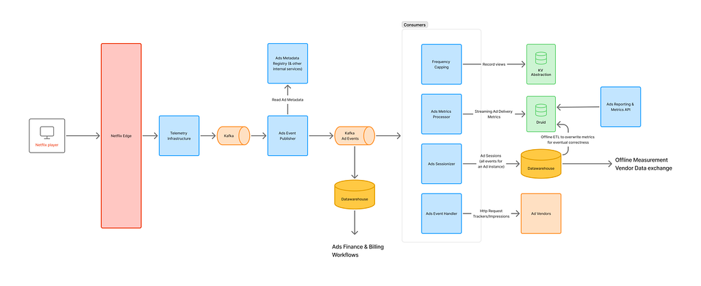
To address these requirements, we implement a solution that combines Lambda for data processing with Jupyter notebooks for analysis, both powered by PyIceberg. This approach provides a lightweight yet robust architecture that maintains data consistency while enabling flexible analysis workflows. At the end of the walkthrough, we also query this data using Athena to demonstrate compatibility with multiple Iceberg-supporting tools and show how the architecture can scale.

We walk through the following high-level steps:

  1. Use Lambda to write sample NYC yellow taxi trip data to an Iceberg table on Amazon S3 using PyIceberg with an AWS Glue Iceberg REST endpoint. In a real-world scenario, this Lambda function would be triggered by an event from a queuing component like Amazon Simple Queue Service (Amazon SQS). For more details, see Using Lambda with Amazon SQS.
  2. Analyze table data in a Jupyter notebook using PyIceberg through the AWS Glue Iceberg REST endpoint.
  3. Query the data using Athena to demonstrate Iceberg’s flexibility.

The following diagram illustrates the architecture.

Overall Architecture

When implementing this architecture, it’s important to note that Lambda functions can have multiple concurrent invocations when triggered by events. This concurrent invocation might lead to transaction conflicts when writing to Iceberg tables. To handle this, you should implement an appropriate retry mechanism and carefully manage concurrency levels. If you’re using Amazon SQS as an event source, you can control concurrent invocations through the SQS event source’s maximum concurrency setting.

Prerequisites

The following prerequisites are necessary for this use case:

Set up resources with AWS CloudFormation

You can use the provided CloudFormation template to set up the following resources:

Complete the following steps to deploy the resources:

  1. Choose Launch stack.

  1. For Parameters, pyiceberg_lambda_blog_database is set by default. You can also change the default value. If you change the database name, remember to replace pyiceberg_lambda_blog_database with your chosen name in all subsequent steps. Then, choose Next.
  2. Choose Next.
  3. Select I acknowledge that AWS CloudFormation might create IAM resources with custom names.
  4. Choose Submit.

Build and run a Lambda function

Let’s build a Lambda function to process incoming records using PyIceberg. This function creates an Iceberg table called nyc_yellow_table in the database pyiceberg_lambda_blog_database in the Data Catalog if it doesn’t exist. It then generates sample NYC taxi trip data to simulate incoming records and inserts it into nyc_yellow_table.

Although we invoke this function manually in this example, in real-world scenarios, this Lambda function would be triggered by actual events, such as messages from Amazon SQS. When implementing real-world use cases, the function code must be modified to receive the event data and process it based on the requirements.

We deploy the function using container images as the deployment package. To create a Lambda function from a container image, build your image on CloudShell and push it to an ECR repository. Complete the following steps:

  1. Sign in to the AWS Management Console and launch CloudShell.
  2. Create a working directory.
mkdir pyiceberg_blog
cd pyiceberg_blog
  1. Download the Lambda script lambda_function.py.
aws s3 cp s3://aws-blogs-artifacts-public/artifacts/BDB-5013/lambda_function.py .

This script performs the following tasks:

  • Creates an Iceberg table with the NYC taxi schema in the Data Catalog
  • Generates a random NYC taxi dataset
  • Inserts this data into the table

Let’s break down the essential parts of this Lambda function:

  • Iceberg catalog configuration – The following code defines an Iceberg catalog that connects to the AWS Glue Iceberg REST endpoint:
# Configure the catalog
catalog_properties = {
   "type": "rest",
   "uri": f"https://glue.{region}.amazonaws.com/iceberg",
   "s3.region": region,
   "rest.sigv4-enabled": "true",
   "rest.signing-name": "glue",
   "rest.signing-region": region
}
catalog = load_catalog(**catalog_properties)
  • Table schema definition – The following code defines the Iceberg table schema for the NYC taxi dataset. The table includes:
    • Schema columns defined in the Schema
    • Partitioning by vendorid and tpep_pickup_datetime using PartitionSpec
    • Day transform applied to tpep_pickup_datetime for daily record management
    • Sort ordering by tpep_pickup_datetime and tpep_dropoff_datetime

When applying the day transform to timestamp columns, Iceberg automatically handles date-based partitioning hierarchically. This means a single day transform enables partition pruning at the year, month, and day levels without requiring explicit transforms for each level. For more details about Iceberg partitioning, see Partitioning.

# Table Definition
schema = Schema(
    NestedField(field_id=1, name="vendorid", field_type=LongType(), required=False),
    NestedField(field_id=2, name="tpep_pickup_datetime", field_type=TimestampType(), required=False),
    NestedField(field_id=3, name="tpep_dropoff_datetime", field_type=TimestampType(), required=False),
    NestedField(field_id=4, name="passenger_count", field_type=LongType(), required=False),
    NestedField(field_id=5, name="trip_distance", field_type=DoubleType(), required=False),
    NestedField(field_id=6, name="ratecodeid", field_type=LongType(), required=False),
    NestedField(field_id=7, name="store_and_fwd_flag", field_type=StringType(), required=False),
    NestedField(field_id=8, name="pulocationid", field_type=LongType(), required=False),
    NestedField(field_id=9, name="dolocationid", field_type=LongType(), required=False),
    NestedField(field_id=10, name="payment_type", field_type=LongType(), required=False),
    NestedField(field_id=11, name="fare_amount", field_type=DoubleType(), required=False),
    NestedField(field_id=12, name="extra", field_type=DoubleType(), required=False),
    NestedField(field_id=13, name="mta_tax", field_type=DoubleType(), required=False),
    NestedField(field_id=14, name="tip_amount", field_type=DoubleType(), required=False),
    NestedField(field_id=15, name="tolls_amount", field_type=DoubleType(), required=False),
    NestedField(field_id=16, name="improvement_surcharge", field_type=DoubleType(), required=False),
    NestedField(field_id=17, name="total_amount", field_type=DoubleType(), required=False),
    NestedField(field_id=18, name="congestion_surcharge", field_type=DoubleType(), required=False),
    NestedField(field_id=19, name="airport_fee", field_type=DoubleType(), required=False),
)

# Define partition spec
partition_spec = PartitionSpec(
    PartitionField(source_id=1, field_id=1001, transform=IdentityTransform(), name="vendorid_idenitty"),
    PartitionField(source_id=2, field_id=1002, transform=DayTransform(), name="tpep_pickup_day"),
)

# Define sort order
sort_order = SortOrder(
    SortField(source_id=2, transform=DayTransform()),
    SortField(source_id=3, transform=DayTransform())
)

database_name = os.environ.get('GLUE_DATABASE_NAME')
table_name = os.environ.get('ICEBERG_TABLE_NAME')
identifier = f"{database_name}.{table_name}"

# Create the table if it doesn't exist
location = f"s3://pyiceberg-lambda-blog-{account_id}-{region}/{database_name}/{table_name}"
if not catalog.table_exists(identifier):
    table = catalog.create_table(
        identifier=identifier,
        schema=schema,
        location=location,
        partition_spec=partition_spec,
        sort_order=sort_order
    )
else:
    table = catalog.load_table(identifier=identifier)
  • Data generation and insertion – The following code generates random data and inserts it into the table. This example demonstrates an append-only pattern, where new records are continuously added to track business events and transactions:
# Generate random data
records = generate_random_data()
# Convert to Arrow Table
df = pa.Table.from_pylist(records)
# Write data using PyIceberg
table.append(df)
  1. Download the Dockerfile. It defines the container image for your function code.
aws s3 cp s3://aws-blogs-artifacts-public/artifacts/BDB-5013/Dockerfile .
  1. Download the requirements.txt. It defines the Python packages required for your function code.
aws s3 cp s3://aws-blogs-artifacts-public/artifacts/BDB-5013/requirements.txt .

At this point, your working directory should contain the following three files:

  • Dockerfile
  • lambda_function.py
  • requirements.txt
  1. Set the environment variables. Replace <account_id> with your AWS account ID:
export AWS_ACCOUNT_ID=<account_id>
  1. Build the Docker image:
docker build --provenance=false -t localhost/pyiceberg-lambda .

# Confirm built image
docker images | grep pyiceberg-lambda
  1. Set a tag to the image:
docker tag localhost/pyiceberg-lambda:latest ${AWS_ACCOUNT_ID}.dkr.ecr.${AWS_REGION}.amazonaws.com/pyiceberg-lambda-repository:latest
  1. Log in to the ECR repository created by AWS CloudFormation:
aws ecr get-login-password --region ${AWS_REGION} | docker login --username AWS --password-stdin ${AWS_ACCOUNT_ID}.dkr.ecr.${AWS_REGION}.amazonaws.com
  1. Push the image to the ECR repository:
docker push ${AWS_ACCOUNT_ID}.dkr.ecr.${AWS_REGION}.amazonaws.com/pyiceberg-lambda-repository:latest
  1. Create a Lambda function using the container image you pushed to Amazon ECR:
aws lambda create-function \
--function-name pyiceberg-lambda-function \
--package-type Image \
--code ImageUri=${AWS_ACCOUNT_ID}.dkr.ecr.${AWS_REGION}.amazonaws.com/pyiceberg-lambda-repository:latest \
--role arn:aws:iam::${AWS_ACCOUNT_ID}:role/pyiceberg-lambda-function-role-${AWS_REGION} \
--environment "Variables={ICEBERG_TABLE_NAME=nyc_yellow_table, GLUE_DATABASE_NAME=pyiceberg_lambda_blog_database}" \
--region ${AWS_REGION} \
--timeout 60 \
--memory-size 1024
  1. Invoke the function at least five times to create multiple snapshots, which we will examine in the following sections. Note that we are invoking the function manually to simulate event-driven data ingestion. In real world scenarios, Lambda functions will be automatically invoked with event-driven fashion.
aws lambda invoke \
--function-name arn:aws:lambda:${AWS_REGION}:${AWS_ACCOUNT_ID}:function:pyiceberg-lambda-function \
--log-type Tail \
outputfile.txt \
--query 'LogResult' | tr -d '"' | base64 -d

At this point, you have deployed and run the Lambda function. The function creates the nyc_yellow_table Iceberg table in the pyiceberg_lambda_blog_database database. It also generates and inserts sample data into this table. We will explore the records in the table in later steps.

For more detailed information about building Lambda functions with containers, see Create a Lambda function using a container image.

Explore the data with Jupyter using PyIceberg

In this section, we demonstrate how to access and analyze the data stored in Iceberg tables registered in the Data Catalog. Using a Jupyter notebook with PyIceberg, we access the taxi trip data created by our Lambda function and examine different snapshots as new records arrive. We also tag specific snapshots to retain important ones, and create new tables for further analysis.

Complete the following steps to open the notebook with Jupyter on the SageMaker AI notebook instance:

  1. On the SageMaker AI console, choose Notebooks in the navigation pane.
  2. Choose Open JupyterLab next to the notebook that you created using the CloudFormation template.

notebook list

  1. Download the notebook and open it in a Jupyter environment on your SageMaker AI notebook.

upload notebook

  1. Open uploaded pyiceberg_notebook.ipynb.
  2. In the kernel selection dialog, leave the default option and choose Select.

select kernel

From this point forward, you will work through the notebook by running cells in order.

Connecting Catalog and Scanning Tables

You can access the Iceberg table using PyIceberg. The following code connects to the AWS Glue Iceberg REST endpoint and loads the nyc_yellow_table table on the pyiceberg_lambda_blog_database database:

import pyarrow as pa
from pyiceberg.catalog import load_catalog
import boto3

# Set AWS region
sts = boto3.client('sts')
region = sts._client_config.region_name

# Configure catalog connection properties
catalog_properties = {
    "type": "rest",
    "uri": f"https://glue.{region}.amazonaws.com/iceberg",
    "s3.region": region,
    "rest.sigv4-enabled": "true",
    "rest.signing-name": "glue",
    "rest.signing-region": region
}

# Specify database and table names
database_name = "pyiceberg_lambda_blog_database"
table_name = "nyc_yellow_table"

# Load catalog and get table
catalog = load_catalog(**catalog_properties)
table = catalog.load_table(f"{database_name}.{table_name}")

You can query full data from the Iceberg table as an Apache Arrow table and convert it to a Pandas DataFrame.

scan table

Working with Snapshots

One of the important features of Iceberg is snapshot-based version control. Snapshots are automatically created whenever data changes occur in the table. You can retrieve data from a specific snapshot, as shown in the following example.

working with snapshots

# Get data from a specific snapshot ID
snapshot_id = snapshots.to_pandas()["snapshot_id"][3]
snapshot_pa_table = table.scan(snapshot_id=snapshot_id).to_arrow()
snapshot_df = snapshot_pa_table.to_pandas()

You can compare the current data with historical data from any point in time based on snapshots. In this case, you are comparing the differences in data distribution between the latest table and a snapshot table:

# Compare the distribution of total_amount in the specified snapshot and the latest data.
import matplotlib.pyplot as plt

plt.figure(figsize=(4, 3))
df['total_amount'].hist(bins=30, density=True, label="latest", alpha=0.5)
snapshot_df['total_amount'].hist(bins=30, density=True, label="snapshot", alpha=0.5)
plt.title('Distribution of total_amount')
plt.xlabel('total_amount')
plt.ylabel('relative Frequency')
plt.legend()
plt.show()

matplotlib graph

Tagging snapshots

You can tag specific snapshots with an arbitrary name and query specific snapshots with that name later. This is useful when managing snapshots of important events.

In this example, you query a snapshot specifying the tag checkpointTag. Here, you are using the polars to create a new DataFrame by adding a new column called trip_duration based on existing columns tpep_dropoff_datetime and tpep_pickup_datetime columns:

# retrive tagged snapshot table as polars data frame
import polars as pl

# Get snapshot id from tag name
df = table.inspect.refs().to_pandas()
filtered_df = df[df["name"] == tag_name]
tag_snapshot_id = filtered_df["snapshot_id"].iloc[0]

# Scan Table based on the snapshot id
tag_pa_table = table.scan(snapshot_id=tag_snapshot_id).to_arrow()
tag_df = pl.from_arrow(tag_pa_table)

# Process the data adding a new column "trip_duration" from check point snapshot.
def preprocess_data(df):
    df = df.select(["vendorid", "tpep_pickup_datetime", "tpep_dropoff_datetime", 
                    "passenger_count", "trip_distance", "fare_amount"])
    df = df.with_columns(
        ((pl.col("tpep_dropoff_datetime") - pl.col("tpep_pickup_datetime"))
         .dt.total_seconds() // 60).alias("trip_duration"))
    return df

processed_df = preprocess_data(tag_df)
display(processed_df)
print(processed_df["trip_duration"].describe())

processed-df

Create a new table from the processed DataFrame with the trip_duration column. This step illustrates how to prepare data for potential future analysis. You can explicitly specify the snapshot of the data that the processed data is referring to by using a tag, even if the underlying table has been changed.

# write processed data to new iceberg table
account_id = sts.get_caller_identity()["Account"] 

new_table_name = "processed_" + table_name
location = f"s3://pyiceberg-lambda-blog-{account_id}-{region}/{database_name}/{new_table_name}"

pa_new_table = processed_df.to_arrow()
schema = pa_new_table.schema
identifier = f"{database_name}.{new_table_name}"

new_table = catalog.create_table(
                identifier=identifier,
                schema=schema,
                location=location
            )
            
# show new table's schema
print(new_table.schema())
# insert processed data to new table
new_table.append(pa_new_table)

Let’s query this new table made from processed data with Athena to demonstrate the Iceberg table’s interoperability.

Query the data from Athena

  1. In the Athena query editor, you can query the table pyiceberg_lambda_blog_database.processed_nyc_yellow_table created from the notebook in the previous section:
SELECT * FROM "pyiceberg_lambda_blog_database"."processed_nyc_yellow_table" limit 10;

query with athena

By completing these steps, you’ve built a serverless data processing solution using PyIceberg with Lambda and an AWS Glue Iceberg REST endpoint. You’ve worked with PyIceberg to manage and analyze data using Python, including snapshot management and table operations. In addition, you ran the query using another engine, Athena, which shows the compatibility of the Iceberg table.

Clean up

To clean up the resources used in this post, complete the following steps:

  1. On the Amazon ECR console, navigate to the repository pyiceberg-lambda-repository and delete all images contained in the repository.
  2. On the CloudShell, delete working directory pyiceberg_blog.
  3. On the Amazon S3 console, navigate to the S3 bucket pyiceberg-lambda-blog-<ACCOUNT_ID>-<REGION>, which you created using the CloudFormation template, and empty the bucket.
  4. After you confirm the repository and the bucket are empty, delete the CloudFormation stack pyiceberg-lambda-blog-stack.
  5. Delete the Lambda function pyiceberg-lambda-function that you created using the Docker image.

Conclusion

In this post, we demonstrated how using PyIceberg with the AWS Glue Data Catalog enables efficient, lightweight data workflows while maintaining robust data management capabilities. We showcased how teams can use Iceberg’s powerful features with minimal setup and infrastructure dependencies. This approach allows organizations to start working with Iceberg tables quickly, without the complexity of setting up and managing distributed computing resources.

This is particularly valuable for organizations looking to adopt Iceberg’s capabilities with a low barrier to entry. The lightweight nature of PyIceberg allows teams to begin working with Iceberg tables immediately, using familiar tools and requiring minimal additional learning. As data needs grow, the same Iceberg tables can be seamlessly accessed by AWS analytics services like Athena and AWS Glue, providing a clear path for future scalability.

To learn more about PyIceberg and AWS analytics services, we encourage you to explore the PyIceberg documentation and What is Apache Iceberg?


About the authors

Sotaro Hikita is a Specialist Solutions Architect focused on analytics with AWS, working with big data technologies and open source software. Outside of work, he always seeks out good food and has recently become passionate about pizza.

Shuhei Fukami is a Specialist Solutions Architect focused on Analytics with AWS. He likes cooking in his spare time and has become obsessed with making pizza these days.

Albertson: OSL’s path to sustainability

Post Syndicated from jzb original https://lwn.net/Articles/1020668/

Lance Albertson writes that the
Oregon State University Open Source Lab has been funded for the next
year, following his announcement in April
that the future of OSL was in jeopardy. OSL is now focusing on
becoming self-sustainable long term.

The recent support was amazing for our immediate team needs. But
for the OSL to thrive long-term, we need a sustainable financial
foundation. This is crucial, as the university expects units like ours
to become self-sufficient beyond this current year.

So, our big focus this next year is locking in ongoing support –
think annualized pledges, different kinds of regular income, and other
recurring help. This is vital, especially with potential new data
center costs and hardware needs. Getting this right means we can stop
worrying about short-term funding and plan for the future: investing
in our tech and people, growing our awesome student programs, and
serving the FOSS community. We’re looking for partners, big and small,
who get why foundational open source infrastructure matters and want
to help us build this sustainable future together.

How to manage migration of hsm1.medium CloudHSM clusters to hsm2m.medium

Post Syndicated from Roshith Alankandy original https://aws.amazon.com/blogs/security/how-to-manage-migration-of-hsm1-medium-cloudhsm-clusters-to-hsm2m-medium/

On August 20, 2024, we announced the general availability of the new AWS CloudHSM instance type hsm2m.medium (hsm2). This new type comes with additional features compared to the previous AWS CloudHSM instance type, hsm1.medium (hsm1), such as support for Federal Information Processing Standard (FIPS) 140-3 Level 3, the ability to run clusters in non-FIPS mode, increased storage capacity of 16,666 total keys, and support for mutual transport layer security (mTLS) between the client and CloudHSM.

The hsm1 instance type is reaching end-of-life and will be unavailable for service on December 1, 2025. See the hsm1 deprecation notification.

To address this, starting April 2025, AWS will attempt to automatically migrate existing hsm1 clusters to hsm2. During the migration, the hsm1 cluster will operate in limited-write mode.

If you want to use automatic migration and can accommodate restrictions on operations during the migration, make sure that your environment meets the prerequisites for automatic migration.

If you want to manage the migration yourself, you can do so before the automatic migration begins. In this post, we provide a few options for migration so you can choose the method that’s best for your situation and available resources.

To help facilitate high availability during migration, you can use a blue/green deployment strategy. If high availability isn’t a priority, there are two approaches: one where write operations are restricted and a second where you incur some downtime on operations. We also cover different use cases based on the operations performed during migration and provide rollback strategies.

Important considerations

When planning a migration to hsm2, consider the following:

  • Backup: We recommend keeping a backup of hsm1 until you have confirmed that all the required keys have been migrated to hsm2. You can configure a CloudHSM backup retention policy to manage backups.

    Note: CloudHSM doesn’t delete a cluster’s last backup. See Configuring AWS CloudHSM backup retention policy for more information. You can also share the CloudHSM backups with other AWS accounts as described in Working with shared backups.

  • Availability and rollback: This post presents two main migration approaches. One that preserves availability but might become complex depending on the type of keys used and operations performed during the migration period. The other approach is less complicated but might impact availability for a short time. Choose the migration process based on your availability requirements.
  • Blue/Green strategy: You can use a blue/green deployment strategy using an enterprise-specific method or a CloudHSM multi-cluster configuration.

    Note: Multi-cluster configuration is supported for CloudHSM CLI, JCE, and PKCS11.

  • Client SDK version: Instance type hsm2 is compatible only with Client SDK version 5.9.0 and later. Upgrade your client SDK before starting migration. We recommend using the latest version.
  • Deprecated algorithms: Make sure you’re not using any deprecated algorithms. You won’t be able to migrate to an hsm2 cluster using backup if you’re using any deprecated algorithms. If you’re using 3DES, you can continue to use it in hsm2 non-FIPS clusters only. See How to migrate 3DES keys from a FIPS to a non-FIPS AWS CloudHSM cluster.
  • Known issues: See the known issues with hsm2 to amend your tests and metrics as needed after migration.

Limited availability

There are two options: customer triggered and customer managed. Choose the approach that best fits your requirements. Note that for both options, you need to satisfy the migration criteria. See Prerequisites for migrating to hsm2m.medium.

Customer triggered

You can trigger migration of your hsm1 cluster from the AWS Management Console for CloudHSM or the AWS Command Line Interface (AWS CLI), and AWS will manage the migration process. Follow the detailed steps in Migrating from hsm1.medium to hsm2m.medium. This approach is suitable if you don’t perform frequent write operations such as creating or deleting users or keys. During the migration, the hsm1 cluster enters limited-write mode where write operations will be rejected until migration is complete. Write operations performed by your application, if any, will fail during the migration. Read operations remain unaffected. If a rollback is required, it will be managed by AWS. If necessary, you can roll back the migration within 24 hours of starting it. The customer triggered migration process is straightforward because no configuration changes are required. If your application requires write operations during migration you can follow the customer managed option.

Customer managed

This approach is suitable if you can schedule a brief downtime to perform migration. For this process, you create a new hsm2 cluster using the latest hsm1 backup. After you add the same number of HSMs to the hsm2 cluster as are in the hsm1 cluster, stop the application, reconfigure the CloudHSM client library to hsm2, and restart the application.

  • Create an hsm2 cluster from backup: CloudHSM makes periodic backups of your cluster at least once every 24 hours. If you need a more recent backup, follow the steps in Cluster backups in AWS CloudHSM to trigger a backup. If you created a backup retention policy when you created the cluster, that will determine how long the backups are retained before being purged. The default is 90 days.

    After you have identified the backup, create an hsm2 cluster from the CloudHSM console or AWS CLI. For the console, choose HSM type hsm2m.medium and Cluster source as Restore cluster from existing backup and choose the designated backup of hsm1.

  • Update cluster for high availability: The new hsm2 cluster will have only one HSM instance. You can now add the same number of instances as hsm1 to this cluster. See adding an HSM to CloudHSM cluster. Based on your workload, add more HSMs to the cluster to ensure high availability. This is a good time to review the cluster to be sure that it follows best practices.
  • Reconfigure client SDKs: During the maintenance window, stop your application that is integrated with the CloudHSM client SDK, reconfigure the appropriate client SDK to talk to the new hsm2 cluster, and then restart the application. See Bootstrap the Client SDK to reconfigure the SDKs. An alternative to stopping and reconfiguring existing applications is to launch a new application instance with the CloudHSM client configured to talk to hsm2 and decommission the old application instance.
  • Monitor the application: Monitor your application’s health metrics and logs to verify that operations run against the new hsm2 cluster are successful. If you see increased errors, you can roll back to the hsm1 cluster and contact AWS Support for assistance.
  • Rollback: You can roll back by reconfiguring your application to communicate with the hsm1 cluster, similar to how you configured your application to talk to the hsm2 cluster.
  • Delete the hsm1 cluster: After you’re satisfied with your new hsm2 cluster, you can delete the hsm1 cluster to reduce costs. This action will create a backup that will be retained—CloudHSM doesn’t delete a cluster’s last backup.

High availability

If you need your CloudHSM cluster to be highly available during migration, AWS recommends that you follow the blue/green deployment methodology. The fundamental idea behind blue/green deployment is to shift traffic between two identical environments that are running different versions of a service or application. The blue environment represents the current version serving production traffic—the hsm1 cluster. The green environment is staged in parallel, running a different version of the service—an hsm2 cluster. After the green environment is ready and tested, production traffic is redirected from blue to green. If problems are identified, you can roll back by reverting traffic back to the blue environment.

We discuss two blue/green approaches in this post. Approach 1 uses a load balancer to route traffic between the blue and green configurations. Approach 2 uses CloudHSM multi-cluster configuration and requires application code changes. Each has pros and cons in terms of effort and cost.

If you have already implemented a multi-cluster configuration in your application, you can follow Approach 2; otherwise, we recommend Approach 1.

A few important things to keep in mind when you implement either of these approaches.

  • You need to create the hsm2 cluster from the hsm1 backup as described in Customer managed.
  • If you need to support write operations during migration, you will need to run additional processes to make sure the data is in sync between the blue and green clusters. See Use cases to learn about different scenarios and plan accordingly.

Approach 1

For this approach, you create two separate but identical client environments. One environment (blue) runs the current application and the client SDK that connects to the hsm1 cluster. The other environment (green) runs the same application with the client SDK configured to talk to the hsm2 cluster. You then use a load balancer—such as Application Load Balancer (ALB)—to selectively route traffic between blue and green using the weighted target groups routing feature of ALB or an equivalent feature in your load balancer.

You can start by directing a small percentage of your application traffic to green. When you’re confident that green is performing well and is stable, shift traffic to green and shut down blue.

Figure 1: Blue/green migration architecture

Figure 1: Blue/green migration architecture

The following are the steps of the migration architecture shown in Figure 1:

  1. Create an hsm2 cluster from an hsm1 backup as described in Customer managed. Make sure you create the new cluster in the same Availability Zones as the existing CloudHSM cluster. This will be your green environment.
  2. Spin up new application instances in the green environment and configure them to connect to the new hsm2 cluster.
  3. Add the new client instances to a new target group for the ALB.
  4. Next, use the weighted target groups routing feature of ALB to route traffic to the newly configured environment.
    1. Each target group weight is a value from 0 to 999. Requests that match a listener rule with weighted target groups are distributed to these target groups based on their weights.
    2. For more information, see Fine-tuning blue/green deployments on application load balancer.

You can follow the canary deployment pattern to roll out an hsm2 cluster integrated application to a subset of users before making it widely available while the hsm1 integrated application serves most of the users. To start, you can configure blue target group with a weight of 90 and green with 10; the ALB will route 90 percent of the traffic to the blue target group and 10 percent to green.

Monitor applications to verify that operations to green are successful (see Monitoring). After you’re satisfied with the response from green, you can update the weights to 0 and 100 for blue and green to completely switch over to green and then shut down blue.

For alternate approaches, such as DNS weighted distribution, see Blue/Green Deployments on AWS

Approach 2

This approach uses a single application environment that talks to both the hsm1 and hsm2 clusters. To shift traffic between blue and green environments, you will use the CloudHSM multi-cluster configuration, which allows a single client SDK to communicate with two or more CloudHSM clusters. Your application code needs to be modified to communicate with both blue and green clusters. In this post, we use a JCE SDK multi-cluster configuration, shown in Figure 2 that follows.

Figure 2: Multi-cluster migration architecture

Figure 2: Multi-cluster migration architecture

The solution uses the basic blue/green deployment steps using a multi-cluster configuration and is designed for common use cases based on the type of CloudHSM operations performed during migration. We also cover how keys can be synchronized between the blue and green clusters and how to roll back.

Create an hsm2 cluster from an hsm1 backup

As described in Customer managed, create an hsm2 cluster from an hsm1 backup. Make sure you create the new cluster in the same Availability Zones as the existing CloudHSM cluster. This will be your green environment.

Modify the application to talk to both blue and green

In this step, you modify the application to use multi-cluster configuration to talk to both blue and green. When using a multi-cluster configuration, you need to configure the CloudHSM provider in the code instead of using the default config file.

In the application code, instantiate two providers: providerHsm1 pointing to blue cluster and providerHsm2 pointing to green cluster. Then update the business logic to switch traffic between blue and green using these providers.

  • Instantiate providers as shown in the following example. See Connecting to multiple clusters with CloudHSM CLI for a detailed explanation. Replace the following:
    • <hsmCAFilePath>: File path to hsm1 trust anchor certificate that you used to initialize the cluster.
    • <hsm1ClusterID>: The unique cluster ID of the hsm1 cluster.
    • <hsm2ClusterID>: The unique cluster ID of the hsm2 cluster.
    CloudHsmProviderConfig hsm1Config = CloudHsmProviderConfig.builder() 
    .withCluster( 
    CloudHsmCluster.builder() 
    .withHsmCAFilePath(<hsmCAFilePath>)
    .withClusterUniqueIdentifier("<hsm1ClusterID>")
    .withServer(CloudHsmServer.builder().withHostIP(hsm1HostName).build()) 
    .build()) 
    .build();
    CloudHsmProvider providerHsm1 = new CloudHsmProvider(hsm1Config);
    
       if (Security.getProvider(provider1.getName()) == null) {.  
                     Security.addProvider(provider1);
         }
    
    CloudHsmProviderConfig hsm2Config = CloudHsmProviderConfig.builder() 
    .withCluster( 
    CloudHsmCluster.builder() 
    .withHsmCAFilePath(<hsmCAFilePath>)
    .withClusterUniqueIdentifier("<sm2ClusterID>")
    .withServer(CloudHsmServer.builder().withHostIP(hsm2HostName).build()) 
    .build()) 
    .build();
    
    CloudHsmProvider providerHsm2 = new CloudHsmProvider(hsm2Config);
    
    if (Security.getProvider(provider2.getName()) == null) { 
                  Security.addProvider(provider2);
    }
    

  • Direct operations to blue and green using the respective providers.
    Cipher cipher1 = Cipher.getInstance("AES/GCM/NoPadding", providerHsm1);
    
    Cipher cipher2 = Cipher.getInstance("AES/GCM/NoPadding", providerHsm2);
    

Switch to green and shut down blue

Monitor the application to verify that operations on green are successful. See the Monitoring section. Once you are satisfied with response from green, you can update the application code to completely switch over to green.

Monitoring

During migration to hsm2, it’s important to monitor your application to confirm it’s working as expected and roll back if you notice increased errors. You can use your application logs and the CloudHSM client SDK logs to monitor the application.

Note: There are some known issues with hsm2 that will be fixed in future releases. See Known issues for AWS CloudHSM hsm2m.medium instances for a list of current known issues and their resolution status.

Use cases

Depending on the type of operations you perform on your CloudHSM cluster during migration, you need to run additional processes to make sure the data is in sync between the blue and green clusters. This will help avoid the split-brain scenario where blue and green clusters are in an inconsistent state if a write operation is performed during migration.

Read-only operations

During migration, if you only need to perform read operations—meaning you aren’t creating token keys—then the data between the clusters will be consistent. You can switch over to green completely following the blue/green-deployment methodology in Approach 1 or Approach 2.

Create/delete operations

If token keys need to be created during migration, the blue and green clusters need to be synchronized to make sure that read operations to the clusters are successful.

  • Write to blue: Initially, create operations can be directed to blue and read operations to both blue and green. In this case, the newly created keys need to be replicated to green. You can use the CloudHSM CLI key replicate command to synchronize keys. See Replicate keys.
  • Write to green: After you gain confidence in the read capability of the green cluster, you could begin swapping over the application to do write operations against the green cluster. In this case, if you’re still reading from both blue and green, you can replicate keys to blue using the CloudHSM CLI key replicate. See Replicate keys.

Replicate keys

Keys can be replicated between CloudHSM clusters that are created from the same backup using CloudHSM CLI with multi-cluster configuration.

Step 1: Configure multi-cluster:

Add blue and green clusters to the multi-cluster configuration. See Connecting to multiple clusters with CloudHSM CLI.

Step 2: Replicate keys from source to destination

Make sure that key owners and users that the key is shared with exist in the destination. Also, the crypto user or admin performing the operation needs to sign in to both clusters.

Run the key replicate command to replicate the keys from blue to green or vice versa as shown in the following example.

  • List keys in hsm1:
    crypto_user@cluster-<hsm1ClusterID> > key list --cluster-id cluster-<hsm1ClusterID>
    

  • List keys in hsm2:
    crypto-user@cluster-<hsm1ClusterID> > key list --cluster-id cluster-<hsm2ClusterID>
    

  • Replicate keys:
    crypto_user@cluster-<hsm1ClusterID> > key replicate \
    --filter attr.label=example-aes-2 \
    --source-cluster-id cluster-<hsm1ClusterID> \
    --destination-cluster-id cluster-<hsm2ClusterID>
    

Rollback

The complexity of a rollback will depend on the stage of the migration and what keys were created. Normally, whether it’s during the migration or after, if you aren’t using hsm2-specific features such as new key attributes, then the rollback is straightforward. During the migration, if a rollback is needed, you can point your application back toward the hsm1 cluster. Through this approach, reads and writes will revert to happening on just the hsm1 and the rollback will be complete. If you created keys in only hsm2, you can replicate them back to hsm1.

The other scenario for a rollback is if you cannot replicate keys back to the hsm1 cluster. This can happen if you have fully migrated your application to hsm2 and have created more than 3,300 keys (the limit for hsm1) or are using hsm2-specific features. In this scenario, you need to make application changes to return to a multi-cluster setup where reads are performed against both hsm1 and hsm2 clusters (in case the keys exist in only hsm2), but write operations happen solely on the hsm1. In this case, the recommendation is to continue talking to both clusters and keep them in sync until non-replicable keys are no longer needed and the cluster can be scaled back down.

Conclusion

In this post, we described strategies to migrate a hsm1.medium CloudHSM cluster to hsm2m.medium. We explored commonly used blue/green deployments and AWS CloudHSM provided options. We also explored common use cases, steps to avoid common pitfalls, and rollback options.

If you have feedback about this post, submit comments in the Comments section below. If you have questions about this post, contact AWS Support.

Roshith Alankandy

Roshith is a Security Consultant at AWS, based in Australia. He helps customers accelerate their cloud adoption journey with security, risk, and compliance guidance and specializes in cryptography. When not working, he enjoys spending time with his family and playing football.

Security updates for Friday

Post Syndicated from daroc original https://lwn.net/Articles/1020653/

Security updates have been issued by Debian (fossil, libapache2-mod-auth-openidc, and request-tracker4), Fedora (thunderbird), Mageia (firefox and thunderbird), SUSE (389-ds, apparmor, cargo-c, chromium, go1.24, govulncheck-vulndb, java-1_8_0-openjdk, kanidm, libsoup, mozjs102, openssl-1_1, openssl-3, python-Django, sccache, tealdeer, tomcat, transfig, wasm-bindgen, and wireshark), and Ubuntu (libreoffice and python-h11).

The collective thoughts of the interwebz