Run Apache Spark and Apache Iceberg write jobs 2x faster with Amazon EMR

Post Syndicated from Atul Payapilly original https://aws.amazon.com/blogs/big-data/run-apache-spark-and-apache-iceberg-write-jobs-2x-faster-with-amazon-emr/

Amazon EMR runtime for Apache Spark offers a high-performance runtime environment while maintaining API compatibility with open source Apache Spark and Apache Iceberg table format. Amazon EMR on EC2, Amazon EMR Serverless, Amazon EMR on Amazon EKS, Amazon EMR on AWS Outposts and AWS Glue use the optimized runtimes.

In this post, we demonstrate the write performance benefits of using the Amazon EMR 7.12 runtime for Spark and Iceberg compares to open source Spark 3.5.6 with Iceberg 1.10.0 tables on a 3TB merge workload.

Write Benchmark Methodology

Our benchmarks demonstrate that Amazon EMR 7.12 can run 3TB merge workloads over 2 times faster than open source Spark 3.5.6 with Iceberg 1.10.0, delivering significant improvements for data ingestion and ETL pipelines while providing the advanced features of Iceberg including ACID transactions, time travel, and schema evolution.

Benchmark workload

To evaluate the write performance improvements in Amazon EMR 7.12, we chose a merge workload that reflects common data ingestion and ETL patterns. The benchmark consists of 37 basic merge operations on TPC-DS 3TB tables, testing the performance of INSERT, UPDATE, and DELETE operations. The workload is inspired by established benchmarking approaches from the open source community, including Delta Lake’s merge benchmark methodology and the LST-Bench framework. We combined and adapted these approaches to create a comprehensive test of Iceberg write performance on AWS. We also started with an initial focus on copy-on-write performance only.

Workload characteristics

The benchmark executes 37 basic sequential merge queries that modify TPC-DS fact tables. The 37 queries are organized into three categories:

  • Inserts (queries m1-m6): Adding new records to tables with varying data volumes. These queries use source tables with 5-100% new records and zero matches, testing pure insert performance at different scales.
  • Upserts (queries m8-m16): Modifying existing records while inserting new ones. These upsert operations combine different ratios of matched and non-matched records—for example, 1% matches with 10% inserts, or 99% matches with 1% inserts—representing typical scenarios where data is both updated and augmented.
  • Deletes (queries m7, m17-m37): Removing records with varying selectivity. These range from small, targeted deletes affecting 5% of files and rows to large-scale deletions, including partition-level deletes that can be optimized to metadata-only operations.

The queries operate on the table state created by previous operations, simulating real ETL pipelines where subsequent steps depend on earlier transformations. For example, the first six queries insert between 607,000 and 11.9 million records into the web_returns table. Later queries then update and delete from this modified table, testing read-after-write performance. Source tables were generated by sampling the TPC-DS web_returns table with controlled match/non-match ratios for consistent test conditions across the benchmark runs.

The merge operations vary in scale and complexity:

  • Small operations affecting 607,000 records
  • Large operations modifying over 12 million records
  • Selective deletes requiring file rewrites
  • Partition-level deletes optimized to metadata operations

Benchmark configuration

We ran the benchmark on identical hardware for both Amazon EMR 7.12 and open source Spark 3.5.6 with Iceberg 1.10.0:

  • Cluster: 9 r5d.4xlarge instances (1 primary, 8 workers)
  • Compute: 144 total vCPUs, 1,152 GB memory
  • Storage: 2 x 300 GB NVMe SSD per instance
  • Catalog: Hadoop Catalog
  • Data format: Parquet files on Amazon S3
  • Table format: Apache Iceberg (default: copy-on-write mode)

Benchmark results

We compared benchmark results for Amazon EMR 7.12 to open source Spark 3.5.6 and Iceberg 1.10.0. We ran the 37 merge queries in three sequential iterations, and the average runtime across these iterations was taken for comparison. The following table shows the results averaged across three iterations:

Amazon EMR 7.12 (seconds) Open Source Spark 3.5.6 + Iceberg 1.10.0 (seconds) Speedup
443.58 926.63 2.08x

The average runtime for the three iterations on Amazon EMR 7.12 with Iceberg enabled was 443.58 seconds, demonstrating a 2.08x speed increase compared to open source Spark 3.5.6 and Iceberg 1.10.0. The following figure presents the total runtimes in seconds.

The following table summarizes the metrics.

Metric Amazon EMR 7.12 on EC2 Open source Spark 3.5.6 and Iceberg 1.10.0
Average runtime in seconds 443.58 926.63
Geometric mean over queries in seconds 6.40746 18.50945
Cost* $1.58 $2.68

*Detailed cost estimates are discussed later in this post.

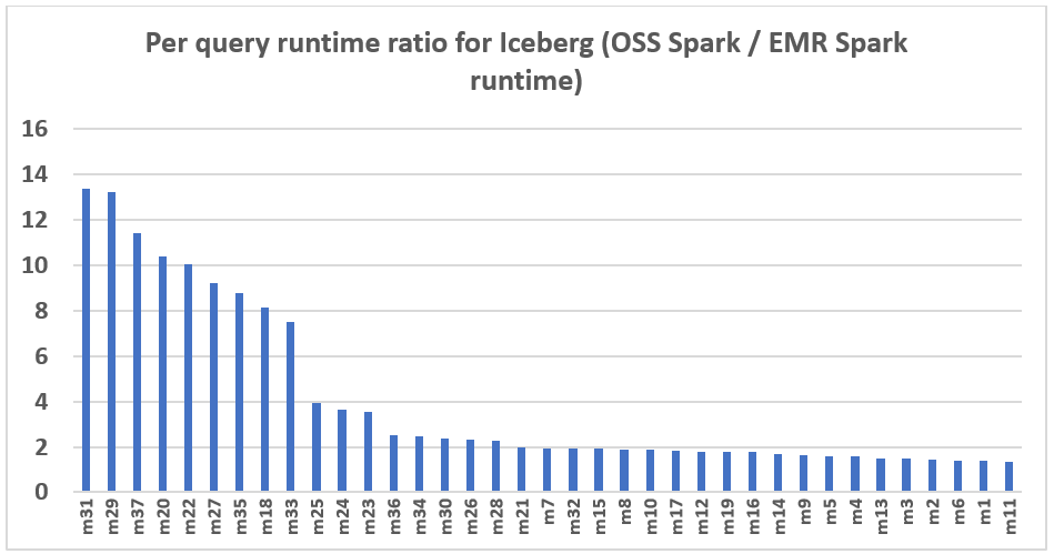
The following chart demonstrates the per-query performance improvement of Amazon EMR 7.12 relative to open source Spark 3.5.6 and Iceberg 1.10.0. The extent of the speedup varies from one query to another, with the fastest up to 13.3 times faster for query m31, with Amazon EMR outperforming open source Spark with Iceberg tables. The horizontal axis arranges the TPC-DS 3TB benchmark queries in descending order based on the performance improvement seen with Amazon EMR, and the vertical axis depicts the magnitude of this speedup as a ratio.

Performance optimizations in Amazon EMR

Amazon EMR 7.12 achieves over 2x faster write performance through systematic optimizations across the write execution pipeline. These improvements span multiple areas:

  • Metadata-only delete operations: When deleting entire partitions, EMR can now optimize these operations to metadata-only changes, eliminating the need to rewrite data files. This significantly reduces the time and cost for partition-level delete operations.
  • Bloom filter joins for merge operations: Enhanced join strategies using bloom filters reduce the amount of data that needs to be read and processed during merge operations, particularly benefiting queries with selective predicates.
  • Parallel file write out: Optimized parallelism during the write phase of merge operations improves throughput when writing filtered results back to Amazon S3, reducing overall merge operation time. We balanced the parallelism with read performance for overall optimized performance on the entire workload.

These optimizations work together to deliver consistent performance improvements across diverse write patterns. The result is significantly faster data ingestion and ETL pipeline execution while maintaining Iceberg’s ACID assurances and data consistency of Iceberg.

Cost comparison

Our benchmark provides the total runtime and geometric mean data to assess the performance of Spark and Iceberg in a complex, real-world decision support scenario. For additional insights, we also examine the cost aspect. We calculate cost estimates using formulas that account for EC2 On-Demand instances, Amazon Elastic Block Store (Amazon EBS), and Amazon EMR expenses.

  • Amazon EC2 cost (includes SSD cost) = number of instances * r5d.4xlarge hourly rate * job runtime in hours
    • 4xlarge hourly rate = $1.152 per hour
  • Root Amazon EBS cost = number of instances * Amazon EBS per GB-hourly rate * root EBS volume size * job runtime in hours
  • Amazon EMR cost = number of instances * r5d.4xlarge Amazon EMR cost * job runtime in hours
    • 4xlarge Amazon EMR cost = $0.27 per hour
  • Total cost = Amazon EC2 cost + root Amazon EBS cost + Amazon EMR cost

The calculations reveal that the Amazon EMR 7.12 benchmark yields a 1.7x cost efficiency improvement over open source Spark 3.5.6 and Iceberg 1.10.0 in running the benchmark job.

Metric Amazon EMR 7.12 Open source Spark 3.5.6 and Iceberg 1.10.0
Runtime in seconds 443.58 926.63
Number of EC2 instances(Includes primary node) 9 9
Amazon EBS Size 20gb 20gb
Amazon EC2(Total runtime cost) $1.28 $2.67
Amazon EBS cost $0.00 $0.01
Amazon EMR cost $0.30 $0
Total cost $1.58 $2.68
Cost savings Amazon EMR 7.12 is 1.7 times better Baseline

Run open source Spark benchmarks on Iceberg tables

We used separate EC2 clusters, each equipped with nine r5d.4xlarge instances, for testing both open source Spark 3.5.6 and Amazon EMR 7.12 for Iceberg workload. The primary node was equipped with 16 vCPU and 128 GB of memory, and the eight worker nodes together had 128 vCPU and 1024 GB of memory. We conducted tests using the Amazon EMR default settings to showcase the typical user experience and minimally adjusted the settings of Spark and Iceberg to maintain a balanced comparison.

The following table summarizes the Amazon EC2 configurations for the primary node and eight worker nodes of type r5d.4xlarge.

EC2 Instance vCPU Memory (GiB) Instance storage (GB) EBS root volume (GB)
r5d.4xlarge 16 128 2 x 300 NVMe SSD 20 GB

Benchmarking instructions

Follow the steps below to run the benchmark:

  1. For the open source run, create a Spark cluster on Amazon EC2 using Flintrock with the configuration described previously.
  2. Setup the TPC-DS source data with Iceberg in your S3 bucket.
  3. Build the benchmark application jar from the source to run the benchmarking and get the results.

Detailed instructions are provided in the emr-spark-benchmark GitHub repository.

Summarize the results

After the Spark job finishes, retrieve the test result file from the output S3 bucket at s3://<YOUR_S3_BUCKET>/benchmark_run/timestamp=xxxx/summary.csv/xxx.csv. This can be done either through the Amazon S3 console by navigating to the specified bucket location or by using the Amazon Command Line Interface (AWS CLI). The Spark benchmark application organizes the data by creating a timestamp folder and placing a summary file within a folder labeled summary.csv. The output CSV files contain four columns without headers:

  • Query name
  • Median time
  • Minimum time
  • Maximum time

With the data from three separate test runs with one iteration each time, we can calculate the average and geometric mean of the benchmark runtimes.

Clean up

To help prevent future charges, delete the resources you created by following the instructions provided in the Cleanup section of the GitHub repository.

Summary

Amazon EMR is consistently enhancing the EMR runtime for Spark when used with Iceberg tables, achieving write performance that is over 2 times faster than open source Spark 3.5.6 and Iceberg 1.10.0 with EMR 7.12 on 3TB merge workloads. This represents a significant improvement for data ingestion and ETL pipelines, helping to deliver 1.7x cost reduction while maintaining the ACID assurances of Iceberg. We encourage you to keep up to date with the latest Amazon EMR releases to fully benefit from ongoing performance improvements.

To stay informed, subscribe to the RSS feed for the AWS Big Data Blog, where you can find updates on the EMR runtime for Spark and Iceberg, as well as tips on configuration best practices and tuning recommendations.


About the authors

Atul Felix Payapilly is a software development engineer for Amazon EMR at Amazon Web Services.

Akshaya KP is a software development engineer for Amazon EMR at Amazon Web Services.

Hari Kishore Chaparala is a software development engineer for Amazon EMR at Amazon Web Services.

Giovanni Matteo is the Senior Manager for the Amazon EMR Spark and Iceberg group.

Medidata’s journey to a modern lakehouse architecture on AWS

Post Syndicated from Mike Araujo original https://aws.amazon.com/blogs/big-data/medidatas-journey-to-a-modern-lakehouse-architecture-on-aws/

This post was co-authored by Mike Araujo Principal Engineer at Medidata Solutions.

The life sciences industry is transitioning from fragmented, standalone tools towards integrated, platform-based solutions. Medidata, a Dassault Systèmes company, is building a next-generation data platform that addresses the complex challenges of modern clinical research. In this post, we show you how Medidata created a unified, scalable, real-time data platform that serves thousands of clinical trials worldwide with AWS services, Apache Iceberg, and a modern lakehouse architecture.

Challenges with legacy architecture

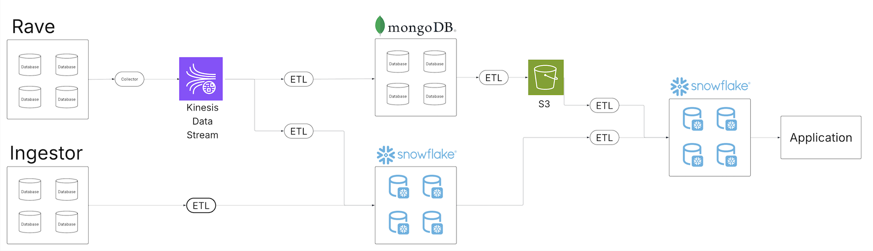
As the Medidata clinical data repository expanded, the team recognized the shortcomings of the legacy data solution to provide quality data products to their customers across their growing portfolio of data offerings. Several data tenants began to erode. The following diagram shows Medidata’s legacy extract, transform, and load (ETL) architecture.

Built upon a series of scheduled batch jobs, the legacy system proved ill-equipped to provide a unified view of the data across the entire ecosystem. Batch jobs ran at different intervals, often requiring a sufficient degree of scheduling buffer to make sure upstream jobs completed within the expected window. As the data volume expanded, the jobs and their schedules continued to inflate, introducing a latency window between ingestion and processing for dependent consumers. Different consumers operating from various underlying data services further magnified the problem as pipelines had to be continuously built across a variety of data delivery stacks.

The expanding portfolio of pipelines began to overwhelm existing maintenance operations. With more operations, the opportunity for failure expanded and recovery efforts further complicated. Existing observability systems were inundated with operational data, and identifying the root cause of data quality issues became a multi-day endeavor. Increases in the data volume required scaling considerations across the entire data estate.

Additionally, the proliferation of data pipelines and copies of the data in different technologies and storage systems necessitated expanding access controls with enhanced security features to make sure only the correct users had access to the subset of data to which they were permitted. Making sure access control changes were correctly propagated across all systems added a further layer of complexity to consumers and producers.

Solution overview

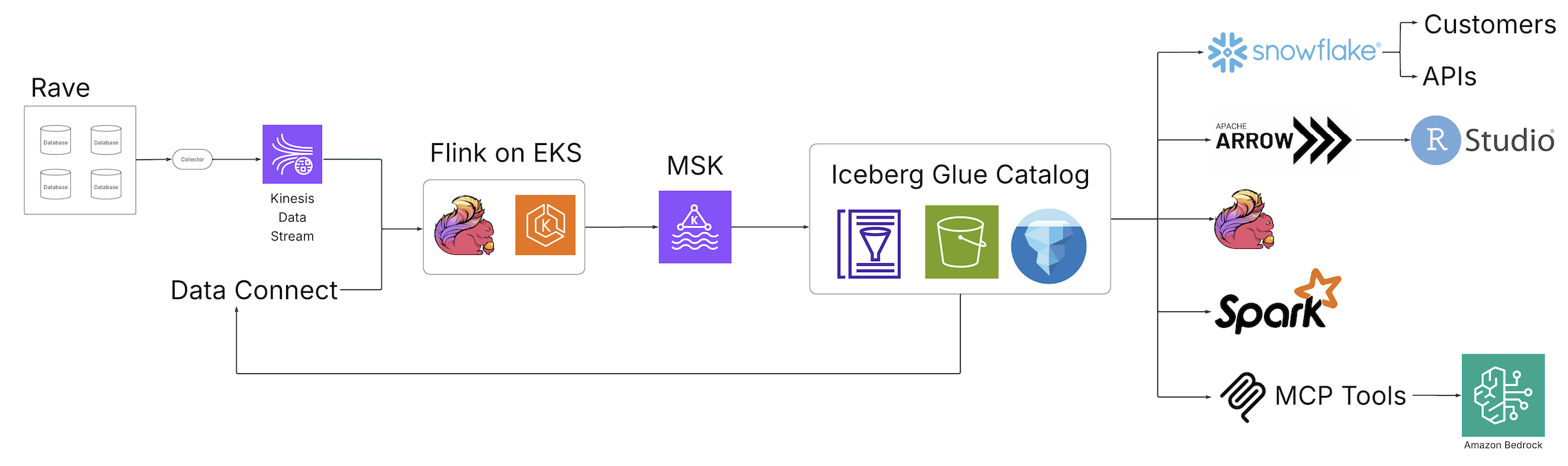
With the advent of Clinical Data Studio (Medidata’s unified data management and analytics solution for clinical trials) and Data Connect (Medidata’s data solution for acquiring, transforming, and exchanging electronic health record (EHR) data across healthcare organizations), Medidata introduced a new world of data discovery, analysis, and integration to the life sciences industry powered by open source technologies and hosted on AWS. The following diagram illustrates the solution architecture.

Fragmented batch ETL jobs were replaced by real-time Apache Flink streaming pipelines, an open source, distributed engine for stateful processing, and powered by Amazon Elastic Kubernetes Service (Amazon EKS), a fully managed Kubernetes service. The Flink jobs write to Apache Kafka running in Amazon Managed Apache Kafka (Amazon MSK), a streaming data service that manages Kafka infrastructure and operations, before landing in Iceberg tables backed by the AWS Glue Data Catalog, a centralized metadata repository for data assets. From this collection of Iceberg tables, a central, single source of data is now accessible from a variety of consumers without additional downstream processing, alleviating the need for custom pipelines to satisfy the requirements of downstream consumers. Through these fundamental architectural changes, the team at Medidata solved the issues presented by the legacy solution.

Data availability and consistency

With the introduction of the Flink jobs and Iceberg tables, the team was able to deliver a consistent view of their data across the Medidata data experience. Pipeline latency was reduced from days to minutes, helping Medidata customers realize a 99% performance gain from the data ingestion to the data analytics layers. Due to Iceberg’s interoperability, Medidata users saw the same view of the data regardless of where they viewed that data, minimizing the need for consumer-driven custom pipelines because Iceberg could plug into existing consumers.

Maintenance and durability

Iceberg’s interoperability provided a single copy of the data to satisfy their use cases, so the Medidata team could focus its observation and maintenance efforts on a five-times smaller subset of operations than previously required. Observability was enhanced by tapping into the various metadata components and metrics exposed by Iceberg and the Data Catalog. Quality management transformed from cross-system traces and queries to a single analysis of unified pipelines, with an added benefit of point in time data queries thanks to the Iceberg snapshot feature. Data volume increases are handled with out-of-box scaling supported by the entire infrastructure stack and AWS Glue Iceberg optimization features that include compaction, snapshot retention, and orphan file deletion, which provide a set-and-forget experience for solving a number of common Iceberg frustrations, such as the small file problem, orphan file retention, and query performance.

Security

With Iceberg at the center of its solution architecture, the Medidata team no longer had to spend the time building custom access control layers with enhanced security features at each data integration point. Iceberg on AWS centralizes the authorization layer using familiar systems such as AWS Identity and Access Management (IAM), providing a single and durable control for data access. The data also stays entirely within the Medidata virtual private cloud (VPC), further reducing the opportunity for unintended disclosures.

Conclusion

In this post, we demonstrated how legacy universe of consumer-driven custom ETL pipelines can be replaced with a scalable, high-performant streaming lakehouses. By putting Iceberg on AWS at the center of data operations, you can have a single source of data for your consumers.

To learn more about Iceberg on AWS, refer to Optimizing Iceberg tables and Using Apache Iceberg on AWS.


About the authors

Mike Araujo

Mike is a Principal Engineer at Medidata Solutions, working on building a next generation data and AI platform for clinical data and trials. By using the power of open source technologies such as Apache Kafka, Apache Flink, and Apache Iceberg, Mike and his team have enabled the delivery of billions of clinical events and data transformations in near real time to downstream consumers, applications, and AI agents. His core skills focus on architecting and building big data and ETL solutions at scale as well as their integration in agentic workflows.

Sandeep Adwankar

Sandeep is a Senior Product Manager at AWS, who has driven feature launches across Amazon SageMaker, AWS Glue, and AWS Lake Formation. He has led initiatives in Amazon S3 Tables analytics, Iceberg compaction strategies, and AWS Glue Iceberg optimizations. His recent work focuses on generative AI and autonomous systems, including the AWS Glue Data Catalog model context protocol and Amazon Bedrock structured knowledge bases. Based in the California Bay Area, he works with customers around the globe to translate business and technical requirements into products that accelerate their business outcomes.

Ian Beatty

Ian is a Technical Account Manager at AWS, where he specializes in supporting independent software vendor (ISV) customers in the healthcare and life sciences (HCLS) and financial services industry (FSI) sectors. Based in the Rochester, NY area, Ian helps ISV customers navigate their cloud journey by maintaining resilient and optimized workloads on AWS. With over a decade of experience building on AWS since 2014, he brings deep technical expertise from his previous roles as an AWS Architect and DevSecOps team lead for SaaS ISVs before joining AWS more than 3 years ago.

Ashley Chen

Ashley is a Solutions Architect at AWS based in Washington D.C. She supports independent software vendor (ISV) customers in the healthcare and life sciences industries, focusing on customer enablement, generative AI applications, and container workloads.

Achieve 2x faster data lake query performance with Apache Iceberg on Amazon Redshift

Post Syndicated from Kalaiselvi Kamaraj original https://aws.amazon.com/blogs/big-data/achieve-2x-faster-data-lake-query-performance-with-apache-iceberg-on-amazon-redshift/

With the growing adoption of open table formats like Apache Iceberg, Amazon Redshift continues to advance its capabilities for open format data lakes. In 2025, Amazon Redshift delivered several performance optimizations that improved query performance over twofold for Iceberg workloads on Amazon Redshift Serverless, delivering exceptional performance and cost-effectiveness for your data lake workloads.

In this post, we describe some of the optimizations that led to these performance gains. Data lakes have become a foundation of modern analytics, helping organizations store vast amounts of structured and semi-structured data in cost-effective data formats like Apache Parquet while maintaining flexibility through open table formats. This architecture creates unique performance optimization opportunities across the entire query processing pipeline.

Performance enhancements

Our latest enhancements span multiple areas of the Amazon Redshift SQL query processing engine, including vectorized scanners that accelerate execution, optimal query plans powered by just-in-time (JIT) runtime statistics, distributed Bloom filters, and new decorrelation rules.

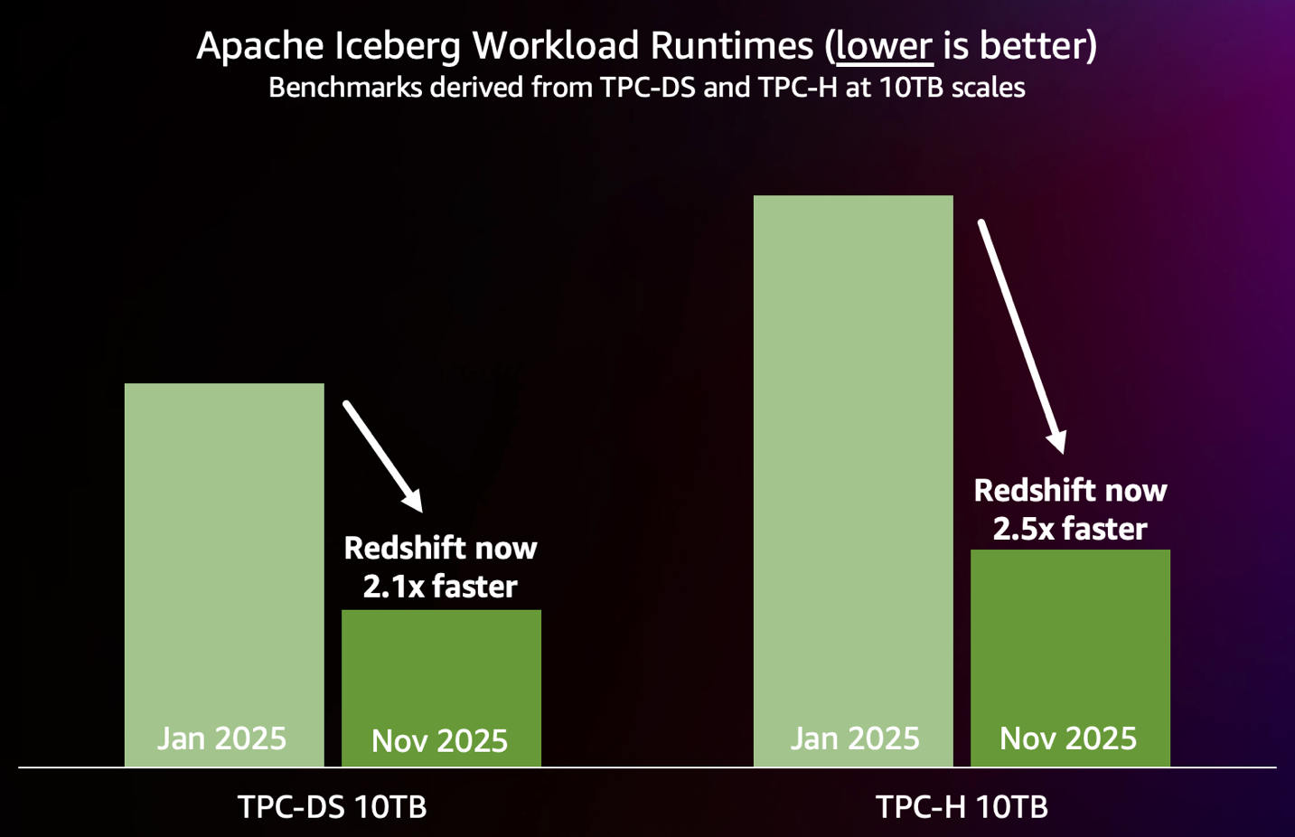
The following chart summarizes the performance improvements achieved so far in 2025, as measured by industry standard 10 TB TPC-DS and TPC-H benchmarks run on Iceberg tables on an 88 RPU Redshift Serverless endpoint.

Find the best performance for your workloads

The performance results presented in this post are based on benchmarks derived from the industry-standard TPC-DS and TPC-H benchmarks, and have the following characteristics:

  • The schema and data of Iceberg tables are used unmodified from TPC-DS. Tables are partitioned to reflect real-world data organization patterns.
  • The queries are generated using the official TPC-DS and TPC-H kits with query parameters generated using the default random seed of the kits.
  • The TPC-DS test includes all 99 TPC-DS SELECT queries. It doesn’t include maintenance and throughput steps. The TPC-H test includes all 22 TPC-H SELECT queries.
  • Benchmarks are run out of the box: no manual tuning or stats collection is done for the workloads.

In the following sections, we discuss key performance improvements delivered in 2025.

Faster data lake scans

To improve data lake read performance, the Amazon Redshift team built a completely new scan layer designed from the ground-up for data lakes. This new scan layer includes a purpose-built I/O subsystem, incorporating smart prefetch capabilities to reduce data latency. Additionally, the new scan layer is optimized for processing Apache Parquet files, the most commonly used file format for Iceberg, through fast vectorized scans.

This new scan layer also includes sophisticated data pruning mechanisms that operate at both partition and file levels, dramatically reducing the volume of data that needs to be scanned. This pruning capability works in harmony with the smart prefetch system, creating a coordinated approach that maximizes efficiency throughout the entire data retrieval process.

JIT ANALYZE for Iceberg tables

Unlike traditional data warehouses, data lakes often lack comprehensive table- and column-level statistics about the underlying data, making it challenging for the planner and optimizer in the query engine to choose up-front which execution plan will be most optimal. Sub-optimal plans can lead to slower and less predictable performance.

JIT ANALYZE is a new Amazon Redshift feature that automatically collects and uses statistics for Iceberg tables during query execution—minimizing manual statistics collection while giving the planner and optimizer in the query engine the information it needs to generate optimal query plans. The system uses intelligent heuristics to identify queries that will benefit from statistics, performs fast file-level sampling using Iceberg metadata, and extrapolates population statistics using advanced techniques.

JIT ANALYZE delivers out-of-the-box performance nearly equal to queries that have pre-calculated statistics, while providing the foundation for many other performance optimizations. Some TPC-DS queries improved by 50 times faster with these statistics.

Query optimizations

For correlated subqueries such as those that contain EXISTS/IN clauses, Amazon Redshift uses decorrelation rules to rewrite the queries. In many cases, these decorrelation rules were not producing optimal plans, resulting in query execution performance regressions. To address this, we introduced a new internal join type, SEMI JOIN, and a new decorrelation rule based on this join type. This decorrelation rule helps in producing the most optimal plans, thereby improving execution performance. For instance, one of the TPC-DS queries that contains EXIST clause ran 7 times faster with this optimization.

We introduced distributed Bloom filter optimization for data lake workloads. Distributed Bloom filters create Bloom filters locally in every compute node and then distributes them to every other node. Distributing Bloom filters can significantly reduce the amount of data that needs to be sent over the network for the join by filtering out the tuples earlier. This provides good performance gains for large, complex data lake queries that process and join large amounts of data.

Conclusion

These performance improvements for Iceberg workloads represent a major leap forward in Redshift data lake capabilities. By focusing on out-of-the-box performance, we’ve made it straightforward to achieve exceptional query performance without complex tuning or optimization.

These improvements demonstrate the power of deep technical innovation combined with practical customer focus. JIT ANALYZE reduces the operational burden of statistics management while providing optimal query planning information. The new Redshift data lake query engine on Redshift Serverless was rewritten from the ground up for best-in-class scan performance, and lays the groundwork for more advanced performance optimizations. Semi-join optimizations tackle some of the most challenging query patterns in analytical workloads. You can run complex analytical workloads on your Iceberg data and get fast, predictable query performance.

Amazon Redshift is committed to being the best analytics engine for data lake workloads, and these performance optimizations represent our continued investment in that goal.

To learn more about Amazon Redshift and its performance capabilities, visit the Amazon Redshift product page. To get started with Redshift, you can try Amazon Redshift Serverless and start querying data in minutes without having to set up and manage data warehouse infrastructure. For more details on performance best practices, see the Amazon Redshift Database Developer Guide. To stay up-to-date with the latest developments in Amazon Redshift, subscribe to the What’s New in Amazon Redshift RSS feed.


Special thanks to this post’s contributors: Martin Milenkoski, Gerard Louw, Konrad Werblinski, Mengchu Cai, Mehmet Bulut, Mohammed Alkateb, and Sanket Hase

Introducing catalog federation for Apache Iceberg tables in the AWS Glue Data Catalog

Post Syndicated from Debika D original https://aws.amazon.com/blogs/big-data/introducing-catalog-federation-for-apache-iceberg-tables-in-the-aws-glue-data-catalog/

Apache Iceberg has become the standard choice of open table format for organizations seeking robust and reliable analytics at scale. However, enterprises increasingly find themselves navigating complex multi-vendor landscapes with disparate catalog systems. Managing data across these has become a major challenge for organizations operating in multi-vendor environments. This fragmentation drives significant operational complexity, particularly around access control and governance. Customers using AWS analytics services such as Amazon Redshift, Amazon EMR, Amazon Athena, Amazon SageMaker, and AWS Glue to analyze Iceberg tables in the AWS Glue Data Catalog want to get the same price-performance for workloads in remote catalogs. Simply migrating or replacing these remote catalogs isn’t practical, leaving teams to implement and maintain synchronization processes that continuously replicate metadata across systems, creating operational overhead, escalating costs, and risking data inconsistencies.

AWS Glue now supports catalog federation for remote Iceberg tables in the Data Catalog. With catalog federation, you can query remote Iceberg tables, stored in Amazon Simple Storage Service (Amazon S3) and cataloged in remote Iceberg catalogs, using AWS analytics engines and without moving or duplicating tables. After a remote catalog is integrated, AWS Glue always fetch the latest metadata in the background, so you always have access to the Iceberg metadata through your preferred AWS analytics services. This capability supports both coarse-grained access control and fine-grained permissions through AWS Lake Formation, giving you the flexibility on how and when remote Iceberg tables are shared with data consumers. With integration for Snowflake Polaris Catalog, Databricks Unity Catalog, and other custom catalogs supporting Iceberg REST specifications, you can federate to remote catalogs, discover databases and tables, configure access permissions, and begin querying remote Iceberg data.

In this post, we discuss how to get started with catalog federation for Iceberg tables in the Data Catalog.

Solution overview

Catalog federation uses the Data Catalog to communicate with remote catalog systems to discover catalog objects and Lake Formation to authorize access to their data in Amazon S3. When you query a remote Iceberg table, the Data Catalog discovers the latest table information in the remote catalog at query runtime, getting the table’s S3 location, current schema, and partition information. Your analytics engine (Athena, Amazon EMR, or Amazon Redshift) Your analytics engine (Athena, EMR, or Redshift) then uses this information to access Iceberg data files directly from Amazon S3. And Lake Formation manages access to the table by vending scoped credentials to the table data stored in Amazon S3, allowing the engines to apply fine-grained permissions to the federated table. This approach avoids metadata and data duplication while providing real-time access to remote Iceberg tables through your preferred AWS analytics engines.

The Data Catalog facilitates connectivity to remote catalog systems that support Apache Iceberg by establishing an AWS Glue connection with the remote catalog endpoint. You can connect the Data Catalog to remote Iceberg REST catalogs using OAuth2 or custom authentication mechanisms using an access token. During integration, administrators configure a principal (service account or identity) with the appropriate permissions to access resources in the remote catalog. The AWS Glue connection object uses this configured principal’s credentials to authenticate and access metadata in the remote catalog server. You can also connect the Data Catalog to remote catalogs that use a private link or proxy for isolating and restricting network access. After it’s connected, this integration uses the standardized Iceberg REST API specification to retrieve the most current table metadata information from these remote catalogs. AWS Glue onboards these remote catalogs as federated catalogs within its own catalog infrastructure, enabling unified metadata access across multiple catalog systems.

Lake Formation serves as the centralized authorization layer for managing user access to federated catalog resources. When users attempt to access tables and databases in federated catalogs, Lake Formation evaluates their permissions and enforces fine-grained access control policies.

Beyond metadata authorization, the catalog federation also manages secure access to the actual underlying data files. It accomplishes this through credential vending mechanisms that issue temporary, scope-limited credentials. AWS Glue federated catalogs work with your preferred AWS analytics engines and query services, enabling consistent metadata access and unified data governance across your analytics workloads.

In the following sections, we walk through the steps to integrate the Data Catalog with your remote catalog server:

  1. Set up an integration principal in the remote catalog and provide required access on catalog resources to this principal. Enable OAuth based authentication for the integration principal.
  2. Create a federated catalog in the Data Catalog using the AWS Glue connection. Create an AWS Glue connection that uses the credentials of the integration principal (in Step1) to connect to the Iceberg REST endpoint of the remote catalog. Configure an AWS Identity and Access Management (IAM) role with permission to S3 locations where the remote table data resides. In a cross-account scenario, make sure the bucket policy grants required access to this IAM role. This federated catalog mirrors the catalog object in your remote catalog server.
  3. Discover Iceberg tables in federated catalogs using Lake Formation or AWS Glue APIs. Query Iceberg tables using AWS analytics engines. During query operations, Lake Formation manages fine-grained permission on federated resources and credential vending to underlying data for the end-users.

Prerequisites

Before you begin, verify you have the following setup in AWS:

  • An AWS account.
  • The AWS Command Line Interface (AWS CLI) version 2.31.38 or later installed and configured.
  • An IAM admin role or user with appropriate permissions to the following services:
    • IAM
    • AWS Glue Data Catalog
    • Amazon S3
    • AWS Lake Formation
    • AWS Secrets manager
    • Amazon Athena
  • Create a data lake admin. For instructions, see Create a data lake administrator.

Set up authentication credentials in remote Iceberg catalog

Catalog federation to a remote Iceberg catalog uses the OAuth2 credentials of the principal configured with metadata access. This authentication mechanism allows the AWS Glue Data Catalog to access the metadata of various objects (such as databases, and tables) within the remote catalogs, based on the privileges associated with the principal. To support proper functionality, you must grant the principal with the necessary permissions to read the metadata of these objects. Generate the CLIENT_ID and CLIENT_SECRET to enable OAuth based authentication for the integration principal.

Create AWS Glue catalog federation using connection to remote Iceberg catalog

Create a federated catalog in the Data Catalog that mirrors a catalog object in the remote Iceberg catalog server and is used by the AWS Glue service to federate metadata queries such as ListDatabases, ListTables, and GetTable to the remote catalog. As data lake administrator, you can create a federated catalog in the Data Catalog using an AWS Glue connection object that is registered with AWS Lake Formation.

Configure data source connection for AWS Glue connection

Catalog federation uses an AWS Glue connection for metadata access when you provide authentication and Iceberg REST API endpoint configurations in the remote catalog. The AWS Glue connection supports OAuth2 or custom as the authentication method.

Connect using OAuth2 authentication

For the OAuth2 authentication method, you can provide a client secret either directly as input or stored in AWS Secrets Manager and used by the AWS Glue connection object during authentication. AWS Glue internally manages the token refresh upon expiration. To store the client secret in Secrets manager, complete the following steps:

  1. On the Secrets Manager console, choose Secrets in the navigation pane.
  2. Choose Store a new secret.
  3. Choose Other type of secret, provide the key name as USER_MANAGED_CLIENT_APPLICATION_CLIENT_SECRET, and enter the client secret value.
  4. Choose Next and provide a name for the secret.
  5. Choose Next and choose Store to save the secret.

Connect using custom authentication

For custom authentication, use Secrets Manager to store and retrieve the access token. This access token is created, refreshed, and managed by the customer’s application or system, providing proper control and management over the authentication process. To store the access token in Secrets Manager, complete the following steps:

  1. On the Secrets Manager console, choose Secrets in the navigation pane.
  2. Choose Store a new secret.
  3. Choose Other type of secret and provide the key name as BEARER_TOKEN with the value noted as the access token of the integration principal.
  4. Choose Next and provide a name for the secret.
  5. Choose Next and choose Store to save the secret.

Register AWS Glue connection with Lake Formation

Create an IAM role that Lake Formation can use to vend credentials and attach permission on S3 bucket prefixes where the Iceberg tables are stored. Optionally, if you’re using Secrets Manager to store the client secret or are using a network configuration, you can add permissions for those services to this role. For instruction, refer to Catalog federation to remote Iceberg catalogs.

Complete the following steps to register the connection:

  1. On the Lake Formation console, choose Catalogs in the navigation pane.
  2. Choose Create catalog and select the data source.
  3. Provide the federated catalog details:
    1. Name of the federated catalog.
    2. Catalog name in the remote catalog server and this needs to match the exact catalog name in remote catalog.
  4. Provide AWS Glue connection details. To reuse an existing connection, choose Select existing connection and choose the connection to reuse. For a first-time setup, choose Input new connection configuration and provide the following information:
    1. Provide the AWS Glue connection name.
    2. Provide the remote catalog Iceberg REST API endpoint.
    3. Specify the catalog object casing type. The connection can support uppercase objects through the object hierarchy or lowercase objects.
    4. Configure authentication parameters:
      1. For OAuth2: Provide the client ID and client secret directly or choose the secret where the client secret is stored, token authorization URL, and scope mapped to the credential.
      2. For custom: Provide the secret managed by Secrets Manager where the access token is stored.
      3. Network configuration: If you have a network and/or proxy setup, you can provide this information. Otherwise, leave this section as default.
  5. Register the connection with Lake Formation using the IAM role with access to the bucket where the remote table metadata and data is stored.
  6. Verify the connection by choosing Run test.
  7. After the test is successful, create the catalog.

You can now discover remote objects under the federated catalog. You can onboard other remote catalogs by reusing the existing connection configured to the same external catalog instance.

Query the federated catalog objects using AWS analytical engines

As the data lake administrator, you can now manage access control on databases and tables in a federated catalog using AWS Lake Formation. You can also use tag-based access control to scale your permission model by tagging the resource based on the access control mechanism.

After permissions are granted, an IAM principal or an IAM user can access the federated tables using AWS analytical services including Athena, Amazon Redshift, Amazon EMR, and Amazon SageMaker. Query the federated Iceberg table using Athena as shown in the following example.

Clean up

To avoid incurring ongoing charges, complete the following steps to clean up the resources created during this walkthrough:

  1. Delete the federated catalog in the Data Catalog:
    aws glue delete-catalog \
        --name <your-federated-catalog-name>

  2. Deregister the AWS Glue connection from Lake Formation:
    aws lakeformation deregister-resource \
        --resource-arn <your-glue-connector-arn>

  3. Revoke Lake Formation permissions (if any were granted):
    # List existing permissions first
    aws lakeformation list-permissions \
        --catalog-id <your-account-id> \
        --resource '{
            "Catalog": {}
        }'
    
    # Revoke permissions as needed
    aws lakeformation revoke-permissions \
        --principal '{
            "DataLakePrincipalIdentifier": "<principal-arn>"
        }' \
        --resource '{
            "Database": {
                "CatalogId": "<catalog-id>",
                "Name": "<database-name>"
            }
        }' \
        --permissions ["SELECT", "DESCRIBE"]

  4. Delete the AWS Glue connection:
    aws glue delete-connection \
        --connection-name <your-glue-connection-to-snowflake-account>

  5. Delete IAM roles and policies associated with Lake Formation and the AWS Glue connection:
    # Detach policies from the role
    aws iam detach-role-policy \
        --role-name <your-lakeformation-role-name> \
        --policy-arn <your-lakeformation-policy-arn>
    
    # Delete the custom policy
    aws iam delete-policy \
        --policy-arn <your-lakeformation-policy-arn>
    
    # Delete the role
    aws iam delete-role \
        --role-name <your-lakeformation-role-name>
    # Detach policies from the role
    aws iam detach-role-policy \
        --role-name <your-glue-connection-role-name> \
        --policy-arn <your-glue-connection-policy-arn>
    
    # Delete the custom policy
    aws iam delete-policy \
        --policy-arn <your-glue-connection-policy-arn>
    
    # Delete the role
    aws iam delete-role \
        --role-name <your-glue-connection-role-name>

  6. Delete the Secrets Manager secret:
    # Schedule secret for deletion (7-30 days)
    aws secretsmanager delete-secret \
        --secret-id <your-snowflake-secret>

This teardown guide doesn’t affect the actual metadata in the remote catalog server nor the data in S3 buckets. It only affects the federation configurations in the Data Catalog and Lake Formation. Any corresponding service principals or configurations in the remote catalog server must be addressed separately.

Make sure you follow the teardown steps in the specified order to avoid dependency conflicts. For example, an AWS Glue connection object can’t be deleted if an AWS Glue catalog object is associated with it.

Additionally, make sure you have the necessary permissions to delete these resources.

Conclusion

In this post, we explored how catalog federation addresses the growing challenge of managing Iceberg tables across multi-vendor catalog environments. We walked through the architecture, demonstrating how the Data Catalog communicates with remote catalog systems, including Snowflake Polaris Catalog, Databricks Unity Catalog, and custom Iceberg REST-compliant catalogs, with centralized authorization and credential vending for secure data access. We covered the setup process, including configuring authentication principals, creating federated catalogs using AWS Glue connections, to implementing fine-grained access controls and querying remote Iceberg tables directly from AWS analytics engines.

Catalog federation offers several advantages:

  • Query your Iceberg data where it lives while maintaining security, governance, and price-performance benefits of AWS analytics services
  • Remove operational overheads and costs to maintain synchronization processes
  • Avoid data duplication and inconsistencies
  • Get real-time access to up-to-date table schemas without migrating or replacing existing catalogs.

To learn more, refer to Catalog federation to remote Iceberg catalogs.


About the authors

Debika D

Debika D

Debika is a Senior Product Marketing Manager with Amazon SageMaker, specializing in messaging and go-to-market strategy for lakehouse architecture. She is passionate about all things data and AI.

Srividya Parthasarathy

Srividya Parthasarathy

Srividya is a Senior Big Data Architect on the AWS Lake Formation team. She works with the product team and customers to build robust features and solutions for their analytical data platform. She enjoys building data mesh solutions and sharing them with the community.

Pratik Das

Pratik Das

Pratik is a Senior Product Manager with AWS Lake Formation. He is passionate about all things data and works with customers to understand their requirements and build delightful experiences. He has a background in building data-driven solutions and machine learning systems.

Accelerate data lake operations with Apache Iceberg V3 deletion vectors and row lineage

Post Syndicated from Ron Ortloff original https://aws.amazon.com/blogs/big-data/accelerate-data-lake-operations-with-apache-iceberg-v3-deletion-vectors-and-row-lineage/

Organizations building petabyte-scale data lakes face increasing challenges as their data grows. Batch updates and compliance deletes create a proliferation of positional delete files, slowing downstream data pipelines and driving up storage costs. Tracking data changes for audit trails and incremental processing requires custom, engine-specific implementations that add complexity and maintenance burden. As data volumes scale, these challenges compound, leaving data teams juggling custom solutions and increasing operational costs just to maintain data freshness and compliance.

Apache Iceberg V3 addresses these challenges with two new capabilities: deletion vectors and row lineage. AWS now delivers these capabilities across Apache Spark on Amazon EMR 7.12, AWS Glue, Amazon SageMaker notebooks, Amazon S3 Tables, and the AWS Glue Data Catalog, giving you a complete, integrated V3 experience without custom implementation. This means faster writes, lower storage costs, comprehensive audit trails, and efficient incremental processing, all working seamlessly across your entire data lake architecture.

In this post, we walk you through the new capabilities in Iceberg V3, explain how deletion vectors and row lineage address these challenges, explore real-world use cases across industries, and provide practical guidance on implementing Iceberg V3 features across AWS analytics, catalog, and storage services.

What’s new in Iceberg V3

Iceberg V3 introduces new capabilities and data types. Two key capabilities that address the challenges discussed earlier are deletion vectors and row lineage.

Deletion vectors replace positional delete files with an efficient binary format stored as Puffin files. Instead of creating separate delete files for each delete operation, the deletion vector consolidates these delete references to a single delete vector per data file, rather than a delete reference file per deleted row. During query execution, engines efficiently filter out deleted rows using these compact vectors, maintaining query performance while removing the need to merge multiple delete files.

This avoids write amplification from random batch updates and GDPR compliance deletes, significantly reducing the overhead of maintaining fresh data. High-frequency update workloads can see immediate improvements in write performance and reduced storage costs from fewer small delete files. Additionally, having fewer small delete files reduces table maintenance costs for compaction operations.

Row lineage enables precise change tracking at the row level with full auditability. Row lineage adds metadata fields to each data file that track when rows were created and last modified. The _row_id field uniquely identifies each row, and the _last_updated_sequence_number field tracks the snapshot when the row was last modified. These fields enable efficient change tracking queries without scanning entire tables, and they’re automatically maintained by the Iceberg specification without requiring custom code.

Before row lineage, change tracking in Iceberg provided only the net changes between snapshots, making it difficult to track individual record modifications. Row lineage metadata fields can now be queried to return all incremental changes, giving you full fidelity for auditing data modifications and regulatory compliance. For data transformations, your downstream systems can process changes incrementally, speeding up data pipelines and reducing compute costs for change data capture (CDC) workflows. Row lineage is engine agnostic, interoperable, and built into the Iceberg V3 specification, alleviating the need for custom, engine-specific change tracking implementations.

Real-world use cases

The new Iceberg V3 capabilities address critical challenges across multiple industries:

  • Marketing and advertising services organizations – You can now efficiently handle GDPR right-to-be-forgotten requests and regulatory compliance deletes without the write amplification that previously degraded pipeline performance. Row lineage provides complete audit trails for data modifications, meeting strict regulatory requirements for data governance.
  • Ecommerce platforms processing millions of product updates and inventory changes daily – You can maintain data freshness while reducing storage costs. Deletion vectors enable faster upsert operations, helping teams meet aggressive SLA requirements during peak shopping periods.
  • Healthcare and life sciences companies – You can track patient data modifications with precision for compliance purposes while efficiently processing large-scale genomic datasets. Row lineage provides the detailed change history required for clinical trial audits and regulatory submissions.
  • Media and entertainment providers managing large catalogs of user viewing data – You can efficiently process incremental changes for recommendation engines. Row lineage enables downstream analytics systems to process only changed records, reducing compute costs in incremental processing scenarios.

Get started with Iceberg V3

To take advantage of deletion vectors for optimized writes and row lineage for built-in change tracking in Iceberg V3, set the table property format-version = 3 during table creation. Alternatively, setting this property on an existing Iceberg V2 table atomically upgrades the table without data rewrites. Before creating or upgrading V3 tables, make sure the Iceberg engines in your solution are V3-compatible. Refer to Apache Iceberg V3 on AWS for more details.

Create a new V3 table with Apache Spark on Amazon EMR 7.12

The following code creates a new table named customer_data. Setting the table property format-version = 3 creates a V3 table. If the format-version table property is not explicitly set, a V2 table is created. V2 is currently the Iceberg default table version. Setting write.delete.mode, write.update.mode, and write.merge.mode to merge-on-read configures Spark to write deletion vectors for delete, update, or merge statements performed on the table.

CREATE TABLE customer_data (
customer_id bigint,
name string,
email string,
last_purchase timestamp,
total_spent decimal(10,2)
)
USING iceberg
TBLPROPERTIES (
'format-version' = '3',
'write.delete.mode' = 'merge-on-read',
'write.update.mode' = 'merge-on-read',
'write.merge.mode' = 'merge-on-read'
)

Run the following code to insert records into the customer_data table:

INSERT INTO customer_data VALUES
 (1, 'Alejandro Rosalez', '[email protected]', TIMESTAMP '2025-11-24 18:55:27', 42.97)
,(2, 'Akua Mansa', '[email protected]', TIMESTAMP '2025-11-24 17:55:27', 25.02)
,(3, 'Ana Carolina Silva','[email protected]', TIMESTAMP '2025-11-24 16:55:27', 43.67)
,(4, 'Arnav Desai','[email protected]', TIMESTAMP '2025-11-24 15:55:27', 98.32)
,(5, 'Carlos Salazar','[email protected]', TIMESTAMP '2025-11-24 12:55:27', 76.45)

Delete a record where customer_id = 5 to generate a delete file:

DELETE 
  FROM customer_data 
  WHERE customer_id = 5

Updating a record with the following update statement also generates a delete file:

UPDATE customer_data
  SET name = 'Mansa Akua' 
  WHERE customer_id = 2

The last part of this example queries the manifest’s metadata table to verify delete files were produced:

SELECT added_snapshot_id
      ,sum(added_delete_files_count) as added_delete_files_count 
FROM customer_data.manifests 
GROUP BY added_snapshot_id 
ORDER BY added_snapshot_id

This query will result in three records returned, as shown in the following screenshot. The added_delete_files_count for the first snapshot that inserts records should be 0. The next two snapshots for the corresponding delete and update statements should have 1 each for added_delete_files_count value.

Query row lineage for change tracking

Row lineage is automatically enabled on V3 tables. The following example includes row lineage metadata fields and an example of how to query table changes after a row lineage sequence number:

SELECT
customer_id,
name,
email,
_row_id,
_last_updated_sequence_number
FROM customer_data
WHERE _last_updated_sequence_number > 0
ORDER BY _last_updated_sequence_number, _row_id

Running this query after the previous insert, update, and delete statements returns four records, as shown in the following screenshot. The deleted record is removed. The _last_updated_sequence_number is 3 for the update to customer_id = 2.

Upgrade an existing V2 table

You can upgrade your existing V2 tables to V3 with the following command:

ALTER TABLE existing_customer_data
SET TBLPROPERTIES ('format-version' = '3')

When you upgrade a table from V2 to V3, several important operations occur atomically:

  • A new metadata snapshot is created atomically, resulting in no data loss.
  • Existing Parquet data files are reused without modification.
  • Row-lineage fields (_row_id and _last_updated_sequence_number) are added to the table metadata.
  • The next compaction operation will remove old V2 positional delete files. If new deletion vector files are generated before compaction runs, they will merge existing V2 positional delete files.
  • New modifications will automatically use V3’s deletion vector files.
  • The upgrade does not perform a historical backfill of row-lineage change tracking records.

The upgrade process is synchronous and completes in seconds for most tables. If the upgrade fails, an error message is returned immediately, and the table remains in its V2 state.

Getting the most from Iceberg V3

In this section, we share the key things we’ve learned from customers already using these features.

Know your workload pattern

Deletion vectors work best when you’re doing lots of writes, such as high-frequency updates, batch deletes, or CDC workloads making random non-append-only updates. If you’re writing more than you’re reading, deletion vectors will deliver immediate performance gains. To unlock these benefits, set your table to merge-on-read mode for delete, update, and merge operations.

Let AWS handle compaction

Enable automatic compaction through the Data Catalog or use S3 Tables (on by default). You will get hands-free optimization without building custom maintenance jobs. Deletion vectors produce fewer delete files than positional deletes in Iceberg V2. Given a similar pattern and amount of modified records, V3 compaction should be quicker and cost less than V2.

Understand the importance of row lineage when using the V2 changelog

With the Spark changelog procedure in Iceberg V2, if a row gets inserted and then deleted between snapshots, it disappears from your change feed—you never see it. Iceberg V3 row lineage captures both operations because _last_updated_sequence_number updates on each modification. This full fidelity is important for audit trails and regulatory compliance where you need to prove what happened to every record. Performance-wise, the V2 changelog requires scanning and merging delete files to compute changes—that’s compute you’re paying for on every read. V3 row lineage stores metadata fields directly on each row, so filtering by _last_updated_sequence_number is a simple metadata scan.

Test before you upgrade

Iceberg V3 upgrades are atomic and fast, but test in dev first. Make sure all your query engines support Iceberg V3 before upgrading shared tables—mixing V2 and V3 engines causes headaches. After upgrading, keep a few V2 snapshots around temporarily for time-travel queries while you validate performance.

Conclusion

Iceberg V3 support across AWS analytics, catalog, and storage services marks a significant advancement in data lake capabilities. By combining deletion vectors’ write optimization with row lineage’s comprehensive change tracking, you can build more efficient, auditable, and cost-effective data lakes at scale. The seamless interoperability across AWS services makes sure your data lake architecture remains flexible and future-proof.

To learn more about AWS support for Iceberg V3, refer to Using Apache Iceberg on AWS.

To learn more about building modern data lakes with Iceberg on AWS, refer to Analytics on AWS.


About the authors

Ron Ortloff

Ron Ortloff

Ron is a Principal Product Manager at AWS.

Orchestrating large-scale document processing with AWS Step Functions and Amazon Bedrock batch inference

Post Syndicated from Brian Zambrano original https://aws.amazon.com/blogs/compute/orchestrating-large-scale-document-processing-with-aws-step-functions-and-amazon-bedrock-batch-inference/

Organizations often have large volumes of documents containing valuable information that remains locked away and unsearchable. This solution addresses the need for a scalable, automated text extraction and knowledge base pipeline that transforms static document collections into intelligent, searchable repositories for generative AI applications.

Organizations can automate the extraction of both content and structured metadata to build comprehensive knowledge bases that power retrieval-augmented generation (RAG) solutions while significantly reducing manual processing costs and time-to-value. The architecture not only demonstrates the processing of 500 research papers automatically, but also scales to handle enterprise document volumes cost-effectively through the Amazon Bedrock batch inference pricing model.

Overview

Amazon Bedrock batch inference is a feature of Amazon Bedrock that offers a 50% discount on inference requests. Although Amazon Bedrock schedules and runs the batch job (needing a minimum of 100 inference requests) as capacity becomes available, the inference won’t be real-time. For use cases where you can accommodate minutes to hours of latency, Amazon Bedrock batch inference is a good option.

This post demonstrates how to build an automated, serverless pipeline using AWS Step Functions, Amazon Textract, Amazon Bedrock batch inference, and Amazon Bedrock Knowledge Bases to extract text, create metadata, and load it into a knowledge base at scale. The example solution processes 500 research papers in PDF format from Amazon Science, extracts text using Amazon Textract, generated structured metadata with Amazon Bedrock batch inference and the Amazon Nova Pro model, and loads the final output, including Amazon Bedrock Knowledge Base filter, into an Amazon Bedrock Knowledge Base.

Architecture

This solution uses Step Functions with parallel Amazon Textract job processing through child workflows run by Distributed Map. You can use the concurrency controls offered by Distributed Map to process documents as quickly as possible within your Amazon Textract quotas. Increasing processing speed necessitates adjusting your Amazon Textract quota and updating the Distributed Map configuration. Amazon Bedrock batch inference handles concurrency, scaling, and throttling. This means that you can create the job without managing these complexities.

In this example implementation, the solution processes research papers to extract metadata such as:

  • Code availability and repository locations
  • Dataset availability and access methods
  • Research methodology types
  • Reproducibility indicators
  • Other relevant research attributes

The high-level parts of this solution include:

  • Extracting text from PDF documents with Amazon Textract in parallel, through Step Functions Distributed Map.
  • Analyzing extracted text using Amazon Bedrock batch inference to extract structured metadata.
  • Loading extract text and metadata into a searchable knowledge base using Amazon Bedrock Knowledge Bases with Amazon OpenSearch Serverless.

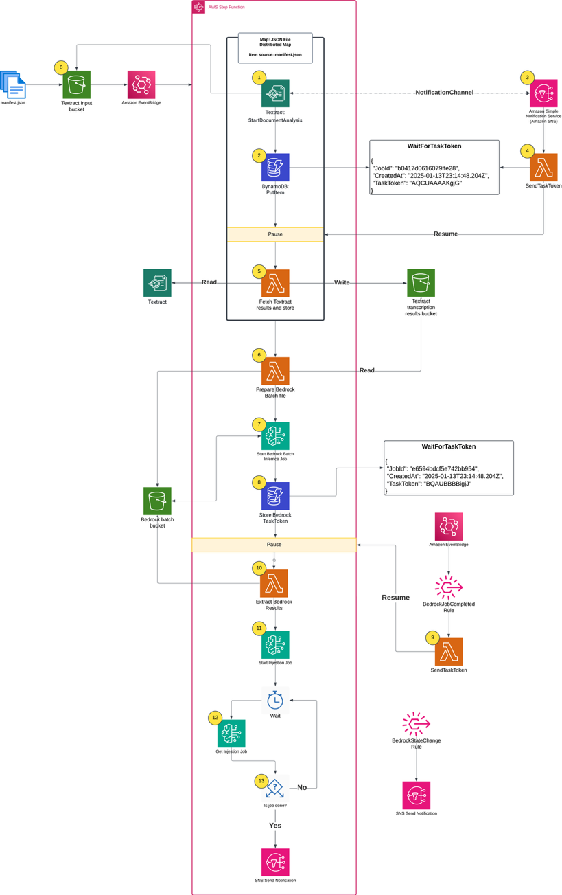
Complete architecture diagram

Figure 1. Complete architecture diagram

Prerequisites

The following prerequisites are necessary to complete this solution:

Running the solution

The complete solution uses AWS CDK to implement two AWS CloudFormation stacks:

  1. BedrockKnowledgeBaseStack: Creates the knowledge base infrastructure
  2. SFNBatchInferenceStack: Implements the main processing workflow

First, clone the GitHub repository into your local development environment and install the requirements:

git clone https://github.com/aws-samples/sample-step-functions-batch-inference.git .

cd sample-step-functions-batch-inference

npm install

Next, deploy the solution using AWS CDK:

cdk deploy --all

After deploying the cdk stacks, upload your data sources (PDF files) into the AWS CDK-created Amazon S3 input bucket. In this example, I uploaded 500 Amazon Science papers. The input bucket name is included in the AWS CDK outputs:

Outputs:

SFNBatchInference.BatchInputBucketName = sfnbatchinference-batchinputbucket11aaa222-nrjki8tewwww

Parallel text extraction

The process begins when you upload a manifest.json file to the input bucket. The manifest file lists the files for processing, which already exist in the input bucket. The filenames listed in manifest.json define what constitutes a single processing job run. To create another run, you would create a different manifest.json and upload it to the same S3 bucket.

[
  {
    "filename": "flexecontrol-flexible-and-efficient-multimodal-control-for-text-to-image-generation.pdf"
  },
  {
    "filename": "adaptive-global-local-context-fusion-for-multi-turn-spoken-language-understanding.pdf"
  }
]

The AWS CDK definition for the input bucket includes Amazon EventBridge notifications and creates a rule that triggers the Step Functions workflow whenever a manifest.json file is uploaded.

private createS3Buckets() {
    const batchBucket = new s3.Bucket(this, "BatchInputBucket", {
      removalPolicy: cdk.RemovalPolicy.DESTROY,
      autoDeleteObjects: true,
    })
    batchBucket.enableEventBridgeNotification()

    new cdk.CfnOutput(this, "BatchInputBucketName", {
      value: batchBucket.bucketName,
      description: "Name of input bucket to send PDF documents that Textract will read.",
    })

    const manifestFileCreatedRule = new eventBridge.Rule(this, "ManifestFileCreatedRule", {
      eventPattern: {
        source: ["aws.s3"],
        detailType: ["Object Created"],
        detail: {
          bucket: {
            name: [batchBucket.bucketName],
          },
          object: {
            key: ["manifest.json"],
          },
        },
      },
    })

    return { batchBucket, manifestFileCreatedRule }
  }

The first step in the Step Functions workflow is a Distributed Map run that performs the following actions for each PDF in the manifest file:

  1. Starts an Amazon Textract job, providing an Amazon Simple Notification Service (Amazon SNS) topic for completion notification.
  2. Writes the Step Functions task token to Amazon DynamoDB, pausing the individual child workflow.
  3. Processes the Amazon SNS message when the Amazon Textract job completes, triggering an AWS Lambda function.
  4. Uses a Lambda function to retrieve the task token from DynamoDB using the Amazon Textract JobId.
  5. Fetches the raw results from Amazon Textract, organizes the text for readability, and writes results to an S3 bucket

First step in the Step Functions workflow

A key component of this architecture is the callback pattern that Amazon Textract supports using the NotificationChannel option, as shown in the preceding figure. The AWS CDK definition the Step Functions state that starts the Amazon Textract job is shown in the following.

const startTextractStep = new tasks.CallAwsService(this, "StartTextractJob", {
  service: "textract",
  action: "startDocumentAnalysis",
  resultPath: "$.textractOutput",
  parameters: {
    DocumentLocation: {
      S3Object: {
        Bucket: sourceBucket.bucketName,
        Name: sfn.JsonPath.stringAt("$.filename"),
      },
    },
    FeatureTypes: ["LAYOUT"],
    NotificationChannel: {
      RoleArn: textractRoleArn,
      SnsTopicArn: snsTopicArn,
    },
  },
  iamResources: ["*"],
})

The Lambda function that handles task tokens extracts the Amazon Textract JobId from the Amazon SNS message, fetches the TaskToken from DynamoDB, and resumes the Step Functions Workflow by sending the TaskToken:

from aws_lambda_powertools.utilities.data_classes import SNSEvent, event_source

@event_source(data_class=SNSEvent)
def handle_textract_task_complete(event, context):
    # Multiple records can be delivered in a single event
    for record in event.records:
        sns_message = json.loads(record.sns.message)
        textract_job_id = sns_message["JobId"]

        # Get both task token and original file from DynamoDB
        ddb_item = _get_item_from_ddb(textract_job_id)

        # Send both the job ID and original file name in the response
        _send_task_success(
            ddb_item["TaskToken"],
            {
                "TextractJobId": textract_job_id,
                "OriginalFile": ddb_item["OriginalFile"],
            },
        )
        # Delete the task token from DynamoDB after use
        _delete_item_from_ddb(textract_job_id)

def _send_task_success(task_token: str, output: None | dict = None) -> None:
    """Sends task success to Step Functions with the provided output"""
    sfn = boto3.client("stepfunctions")
    sfn.send_task_success(taskToken=task_token, output=json.dumps(output or {}))

The Distributed Map runs up to 10 child workflows concurrently, controlled by the maxConcurrency setting. Although Step Functions supports running up to 10,000 child workflow executions, the practical concurrency for this solution is constrained by Amazon Textract quotas. The startDocumentAnalysis API has a default quota of 10 requests per second (RPS), which means you must consider this limit when scaling your document processing workloads and potentially request quota increases for higher throughput requirements.

const distributedMap = new sfn.DistributedMap(this, "DistributedMap", {
  mapExecutionType: sfn.StateMachineType.STANDARD,
  maxConcurrency: 10,
  itemReader: new sfn.S3JsonItemReader({
    bucket: sourceBucket,
    key: "manifest.json",
  }),
  resultPath: "$.files",
}

Running Amazon Bedrock batch inference

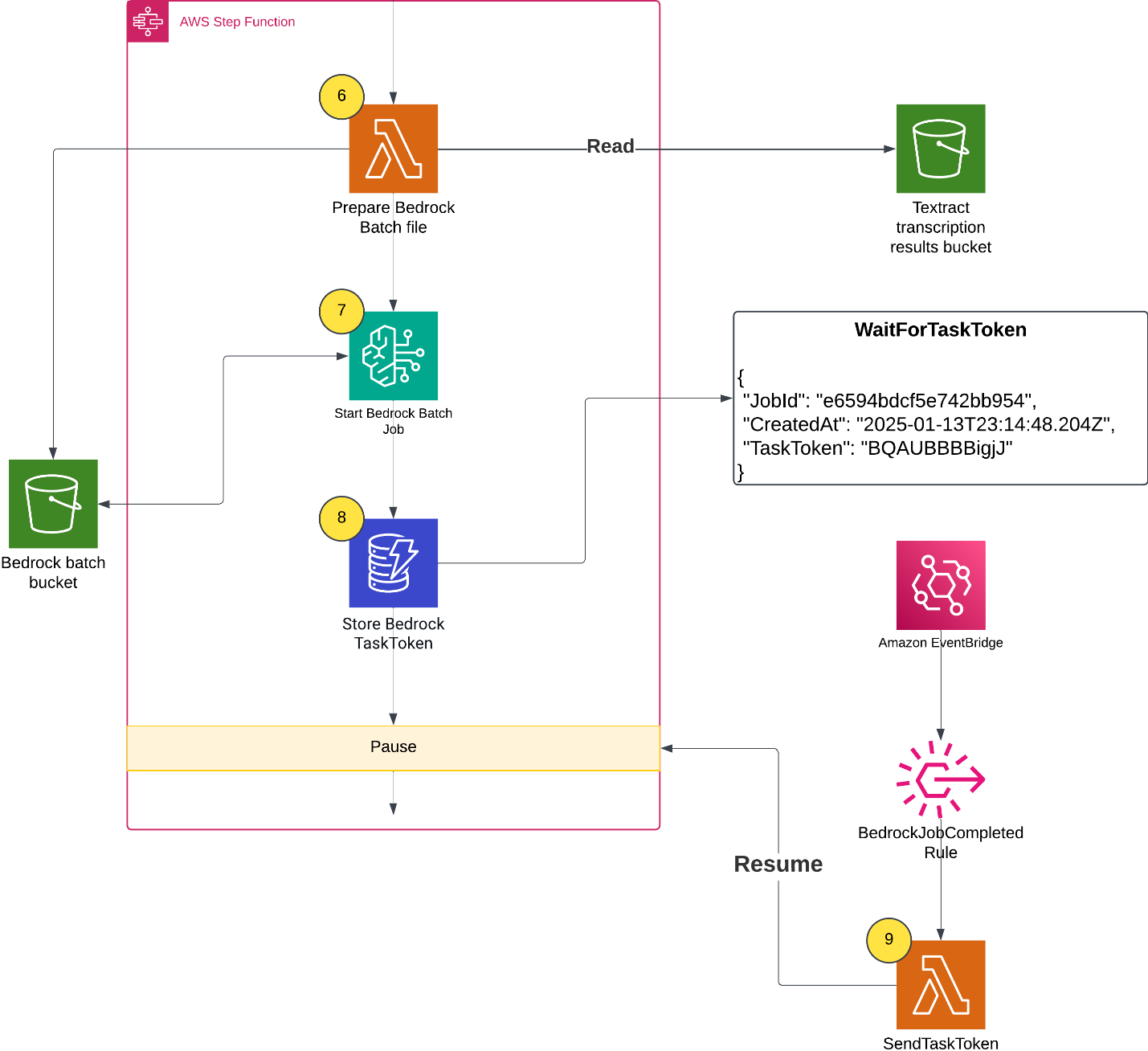
When all of the Amazon Textract jobs finish, the Distributed Map state creates an Amazon Bedrock batch inference input file, launches the Amazon Bedrock inference job, and waits for it to complete.

  1. A Lambda function collects text results from Amazon S3 and creates an Amazon Bedrock batch inference input file with custom prompts.
  2. The workflow starts the Amazon Bedrock batch inference job by calling createModelInvocationJob and sending the batch inference input file as input.
  3. The workflow pauses and stores the task token in DynamoDB.
  4. An EventBridge rule matches completed Amazon Bedrock batch inference events, and upon job completion and triggers a Lambda function. The Lambda function retrieves the task token and resumes the workflow, as shown in the following figure.

Lambda function retrieves the task token and resumes the workflow

A batch inference input is a single jsonl file with multiple entries such as the following example. The prompt in each inference request instructs the large language model (LLM) to analyze the paper and extract metadata. Read the full prompt template in the GitHub repository.

{
  "recordId": "c1b8a3b2086141f963",
  "modelInput": {
    "messages": [
      {
        "role": "user",
        "content": [
          {
            "text": "Analyze the following research paper transcript and extract metadata about code and dataset availability. Extract the following metadata from this research paper transcript:\n\n1. **has_code**: Does the paper mention or link to source code? (true/false) ...... Return only valid JSON matching the schema above. Do not include any text outside of the JSON structure."
          }
        ]
      }
    ],
    "inferenceConfig": { "maxTokens": 4096 }
  }
}

Populating the Amazon Bedrock Knowledge Base

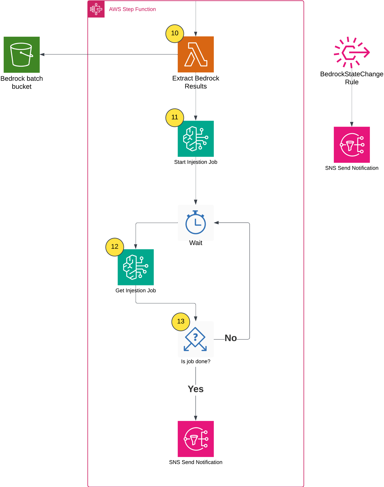
After the batch inference completes, the workflow does the following:

  1. Extracts inference results and creates metadata files based on the Amazon Bedrock inference results (example metadata shown in the following figure).
  2. Starts an Amazon Bedrock Knowledge Base ingestion job.
  3. Monitors the ingestion job status using Step Functions Wait and Choice states.
  4. Sends a completion notification through Amazon SNS.

Populating the Amazon Bedrock Knowledge Base

The following shows the example metadata format:

{
  "metadataAttributes": {
    "has_code": true,
    "has_dataset": false,
    "code_availability": "publicly_available",
    "dataset_availability": "not_available",
    "research_type": "methodology",
    "is_reproducible": true,
    "code_repository_url": "https://github.com/amazon-science/PIXELS"
  }
}

Testing the knowledge base

After the workflow completes successfully, you can test the knowledge base to verify that the documents and metadata have been properly ingested and are searchable. There are two practical methods for testing an Amazon Bedrock Knowledge Base:

  1. Using the Console
  2. Using the AWS SDK to run a query

Testing through the Console

The Console provides an intuitive interface for testing your knowledge base queries with metadata filters:

  1. Navigate to the Amazon Bedrock console.
  2. In the left navigation pane, choose Knowledge Bases under the Build section.
  3. Choose the knowledge base created by the AWS CDK deployment (the name will be output by the AWS CDK stack).
  4. Choose the Test button in the upper right corner.
  5. In the test interface, choose your preferred foundation model (FM) (such as Amazon Nova Pro).
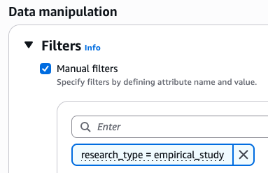
  6. Expand the Configurations column, then navigate to the Filters section.
  7. Configure filters based on the extracted metadata, as shown in the following figure.

Configure filters based on the extracted metadata

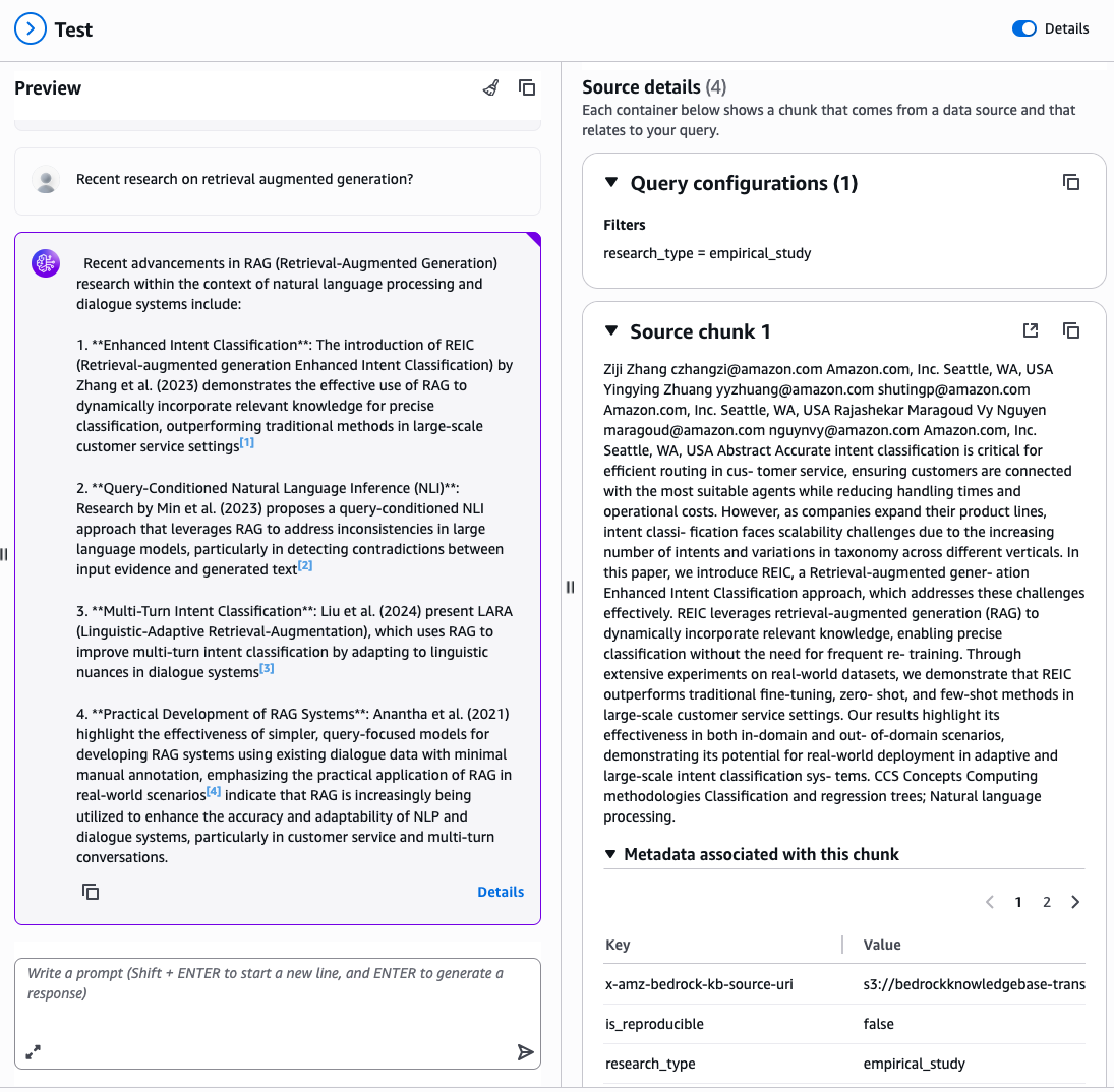
Enter a natural language query related to your documents, for example: “Recent research on retrieval augmented generation?”

The console displays the generated response along with source attributions showing which documents were retrieved and used to formulate the answer, filtered by your specified metadata attributes, as shown in the following figure.

A chat example

Testing via API

For programmatic testing and integration into applications, use the AWS SDK with metadata filtering. The following is a Python example using boto3:

model_arn = "arn:aws:bedrock:us-east-1::foundation-model/amazon.nova-pro-v1:0"

# Query for papers with publicly available code
response = bedrock_agent_runtime.retrieve_and_generate(
    input={'text': "What recent research has been done on RAG?"},
    retrieveAndGenerateConfiguration={
        'type': 'KNOWLEDGE_BASE',
        'knowledgeBaseConfiguration': {
            'knowledgeBaseId': knowledge_base_id,
            'modelArn': model_arn,
            'retrievalConfiguration': {
                'vectorSearchConfiguration': {
                    'numberOfResults': 5,
                    'filter': {"equals": {"key": "has_code", "value": True}},
                }
            },
        },
    },
)

# Display results
print(f"Response: {response['output']['text']}\n")
print("Source Documents:")

for citation in response.get('citations', []):
    for reference in citation.get('retrievedReferences', []):
        metadata = reference.get('metadata', {})
        print(f" Document: {reference['location']['s3Location']['uri']}\n")

The following is the test script output:

Response: Recent research on Retrieval-Augmented Generation (RAG) has focused on enhancing the system's ability to dynamically retrieve and utilize relevant information from a Vector Database (VDB) to improve decision-making and performance. Key innovations include:

1. **Dynamic Retrieval and Utilization**: The system is designed to query the VDB for contextually relevant past experiences, which significantly improves decision quality and accelerates performance by leveraging a growing repository of relevant experiences.

2. **Teacher-Student Instructional Tuning**: A novel mechanism where a Teacher agent refines a Student agent's core policy through direct interaction. The Teacher generates a modified SYSTEM prompt based on the Student's actions, creating a meta-learning loop that enhances the Student's reasoning policy over time.

Conclusion

This solution demonstrates how to combine multiple AWS AI and serverless services to build a scalable document processing pipeline. Organizations can use AWS Step Functions for orchestration, Amazon Textract for document processing, Amazon Bedrock batch inference for intelligent content analysis, and Amazon Bedrock Knowledge Bases for searchable storage. In turn, they can automate the extraction of insights from large document collections while optimizing costs.

Following this solution, you can build a solid foundation for production-scale document processing pipelines that maintain the flexibility to adapt to your specific requirements while making sure of reliability, scalability, and operational excellence. Follow this link to learn more about serverless architectures.

AWS Private Certificate Authority now supports partitioned CRLs

Post Syndicated from Kartik Bhatnagar original https://aws.amazon.com/blogs/security/aws-private-certificate-authority-now-supports-partitioned-crls/

Public Key Infrastructure (PKI) is essential for securing and establishing trust in digital communications. As you scale your digital operations, you’ll issue and revoke certificates. Revoking certificates is useful especially when employees leave, migrate to a new certificate authority hierarchy, meet compliance, and respond to security incidents. Use the Certificate Revocation List (CRL) or Online Certificate Status Protocol (OCSP) method to track revoked certificates. You can use Amazon Web Services (AWS) Private Certificate Authority (AWS Private CA) to create a certificate authority (CA), which publishes revocation information through these methods so that systems can verify certificate validity.

As enterprises continue to scale their operations, they face limitations when using complete CRLs to issue and revoke more than 1 million certificates. The workaround of increasing CRL file sizes isn’t viable, because many applications can’t process large CRL files (with some needing a 1 MB maximum). Furthermore, alternative solutions like OCSP may be rejected by major trust stores and browser vendors due to privacy concerns and compliance requirements. These constraints significantly impact your ability to scale PKI infrastructure efficiently while maintaining security and compliance standards.

Feature release: Addressing challenges

AWS Private CA addresses these challenges with partitioned CRLs, which enable the issuance and revocation of up to 100 million certificates per CA. This feature distributes revocation information across multiple smaller, manageable CRL partitions, each maintaining a maximum size of 1 MB for more effective application compatibility. At the time of issuance, certificates are automatically bound to specific CRL partitions through a critical Issuer Distribution Point (IDP) extension, which contains a unique URI identifying the partition. Validation works by comparing the CRL URI in the certificate’s CRL Distribution Point (CDP) extension against the CRL’s IDP extension, which provides accurate certificate validation.

Partitioned CRL provides automatic scaling of certificate issuance limits from 1M to 100M certificates per CA, support for both new and existing CAs, flexible configuration options for CRL naming and paths, backward compatibility by preserving existing complete CRL functionality while offering partitioned CRL as an optional feature, and compliance with industry standards such as RFC5280 while maintaining security and operational efficiency.

Configuring Partitioned CRLs in AWS Private CA

You can configure Partitioned CRLs for existing CAs in AWS Private CA by using the following steps.

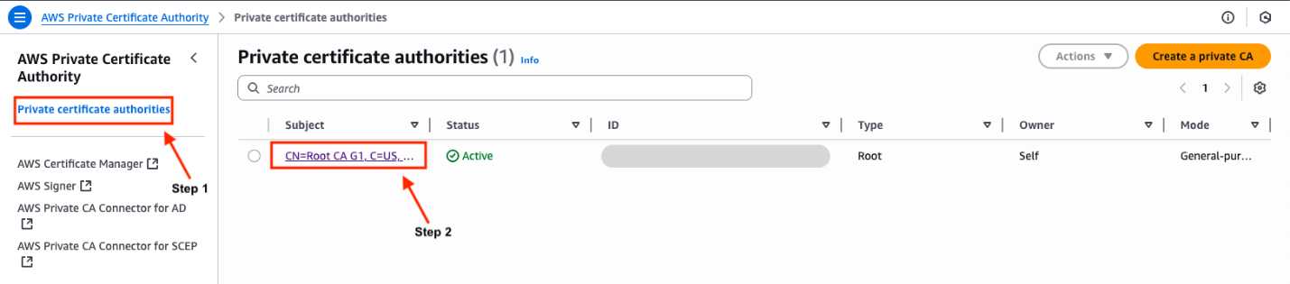
  1. Choose Private certificate authorities in the left navigation bar.
  2. Choose the hyperlink in the Subject column that is your CA to go into its details.

    Note: Verify that you are in the correct AWS Region.

    Figure 1: Certificate Authority selection

    Figure 1: Certificate Authority selection

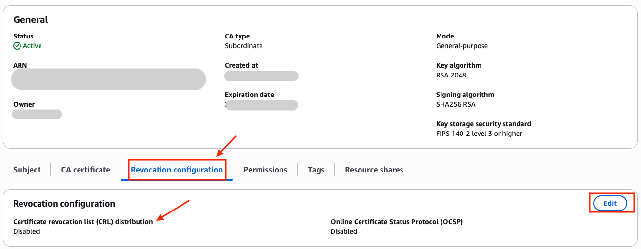
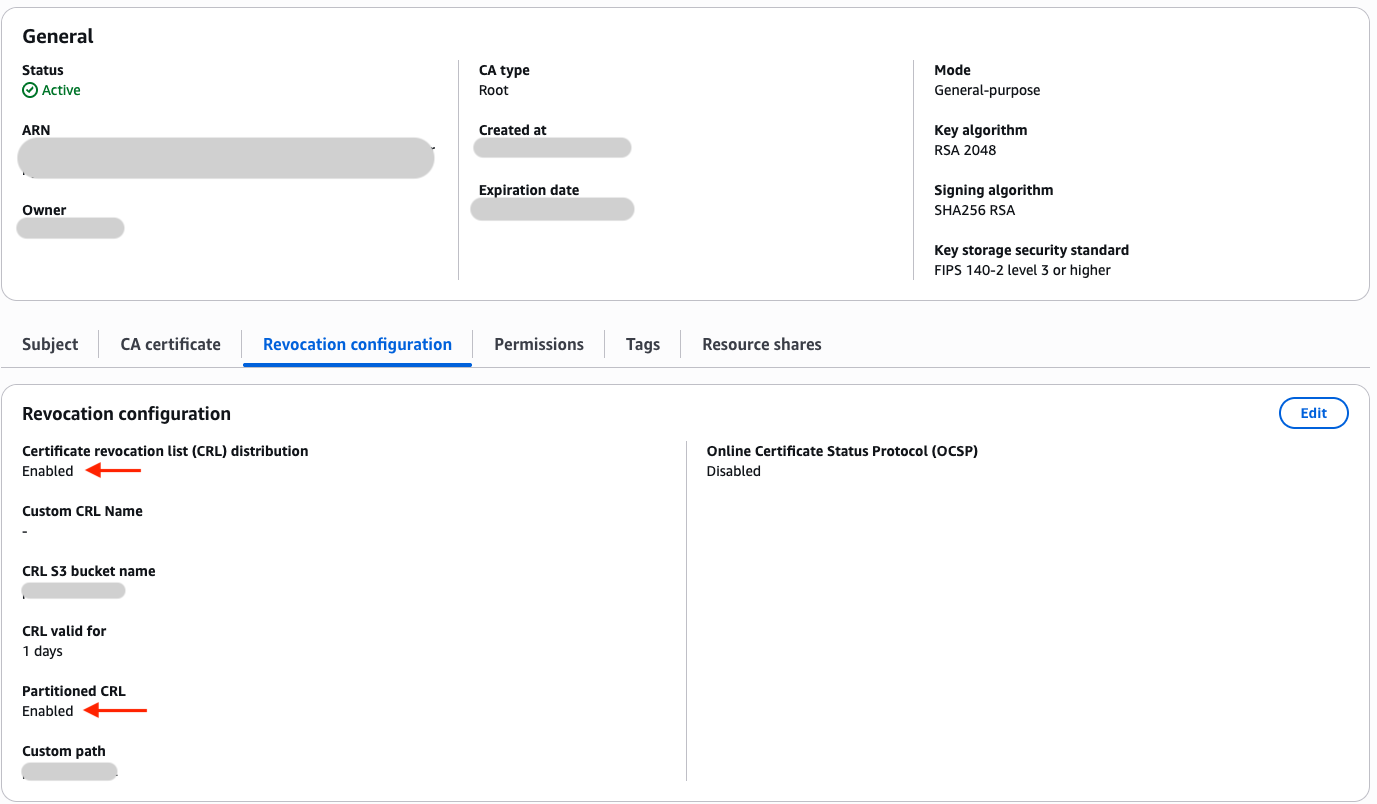
  3. Choose the Revocation configuration tab and you should observe the CRL distribution enabled or disabled. If it is disabled, then you should enable it in the next steps.
    Figure 2: Certification Authority general configuration information

    Figure 2: Certification Authority general configuration information

  4. Choose Edit.
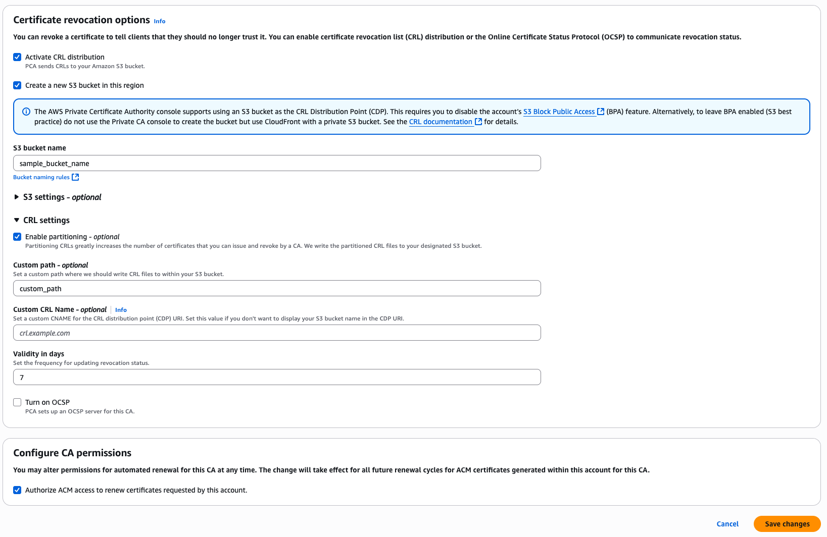
  5. Check the checkbox of Activate CRL distribution.

    If CRL distribution was enabled already, then skip to step 7.

  6. Under S3 bucket URI, choose an existing bucket from the list. You can observe detailed steps listed in Step 6 of the instructions in Create a private CA in AWS Private CA.

    You must verify that BPA is disabled for the account and for the bucket, and you must manually attach a policy to it before you can begin generating CRLs. Use one of the policy patterns described in Access policies for CRLs in Amazon S3. For more information, go to Adding a bucket policy using the Amazon S3 console.

  7. Expand CRL settings for more configuration options.
  8. Check the Enable partitioning checkbox to enable partitioning of CRLs. This creates a partitioned CRL.

    If you don’t enable partitioning, then a complete CRL is created and your CA is subject to the limit of 1M issued or revoked certificates. For more information, go to AWS Private CA quotas.

    Figure 3: Certificate revocation options

    Figure 3: Certificate revocation options

  9. Choose Save changes.
  10. CRL distribution shows as enabled with partitioned CRLs. The limit of 1M automatically updates to 100M per CA.
    Figure 4: Certificate revocation configuration

    Figure 4: Certificate revocation configuration

Conclusion

The AWS Private CA partitioned CRLs can deliver substantial benefits across multiple dimensions. From a security perspective, the feature maintains certificate validation while supporting comprehensive revocation capabilities for up to 100M certificates per CA. Therefore, you can respond effectively to security incidents or key compromises. Operationally, it reduces CA rotation, lessening administrative overhead and streamlining PKI management. Furthermore, maintaining CRL partition sizes at 1 MB provides broad compatibility with applications while supporting automated partition management. Moreover, this makes it particularly valuable when you need scalable, standards-compliant certificate management. Regarding compliance, you can use the feature to comply with multiple industry requirements: it supports WebTrust principles and criteria and ETSI TSP standards, maintains compatibility with RFC5280, aligns with browser trust store requirements for both CRL and OCSP support, and provides the flexibility needed for emerging standards such as Matter.

Lastly, you can maximize the value of your general purpose or short-lived CA while all certificates remain revocable by enabling Partitioned CRL for no added charge on top of AWS Private CA and Amazon Simple Storage Service (Amazon S3).

Start creating your CA in AWS Private CA using AWS Management Console.

If you have feedback about this post, submit comments in the Comments section below.

Kartik Bhatnagar

Kartik Bhatnagar

Kartik is a San Francisco-based Solutions Architect at AWS, specializing in data security. With experience serving both startups and enterprises across fintech, healthcare, and media industries as a DevOps Engineer and Systems Architect, he helps customers design secure, scalable AWS solutions. Off-duty, he enjoys cricket, tennis, food hopping, and hiking.

How Octus achieved 85% infrastructure cost reduction with zero downtime migration to Amazon OpenSearch Service

Post Syndicated from Vaibhav Sabharwal original https://aws.amazon.com/blogs/big-data/how-octus-achieved-85-infrastructure-cost-reduction-with-zero-downtime-migration-to-amazon-opensearch-service/

As data volumes continue to grow exponentially, there is increasing pressure to optimize search infrastructure costs while maintaining the high performance and reliability that mission-critical workloads demand. Many companies find themselves managing complex, expensive search systems that require significant operational overhead and limit their ability to scale efficiently. The challenge becomes even more acute when organizations need to migrate between search systems, a process that traditionally involves substantial downtime, complex data synchronization, and significant impact on business operations. Enterprise applications cannot afford service interruptions that could impact customer experiences, business intelligence, or operational continuity. Migration strategies need to deliver cost optimization and operational improvements while maintaining zero downtime and facilitating complete data integrity throughout the transition process.

Founded in 2013, Octus, formerly Reorg, is the essential credit intelligence and data provider for the world’s leading buy side firms, investment banks, law firms and advisory firms. By surrounding unparalleled human expertise with proven technology, data and AI tools, Octus unlocks powerful truths that fuel decisive action across financial industries.

This post highlights how Octus migrated its Elasticsearch workloads running on Elastic Cloud to Amazon OpenSearch Service. The journey traces Octus’s shift from managing multiple systems to adopting a cost-efficient solution powered by OpenSearch Service. Along the way, we share the architecture choices and implementation strategies that made the migration successful. The result is uninterrupted service availability throughout migration, with improved performance and greater cost efficiency.

Strategic requirements

We identified several requirements that made Amazon OpenSearch Service the right choice for their migration:

  • Cost efficiency: The OpenSearch Service pricing model enabled us to optimize cloud spend without compromising performance.
  • Responsive support: AWS provided dependable, high-quality support to accelerate issue resolution and instill confidence.
  • Consistent reliability: OpenSearch Service provides an SLA up to 99.99% offering the reliability required for Octus’s mission-critical workloads.
  • Seamless migration with no query downtime: Migration Assistant for Amazon OpenSearch Service provided Octus with a migration path while maintaining uninterrupted query availability during the migration, facilitating business continuity.
  • Operational simplification: Consolidating onto AWS reduced infrastructure complexity while maintaining high security standards.

Solution overview

The Migration Assistant for Amazon OpenSearch Service provides a suite of tools to aid in Elasticsearch to OpenSearch Service migrations. Octus use the following capabilities for their migration:

  • Metadata migration: The tool enabled Octus to migrate dozens of indices with diverse mappings and settings. When a backward incompatibility was identified with timestamp metadata, a custom JavaScript transformation, integrated directly into the Migration Assistant tooling, was applied to automatically adjust the mappings across the indices and facilitate compatibility.
  • Historical data migration: Octus used Reindex-from-Snapshot to migrate the historical documents from a point-in-time snapshot of the source cluster, scaling this process without impacting the source cluster since the snapshot was stored in Amazon Simple Storage Service (Amazon S3). Reindex-from-Snapshot also enabled Octus to adjust the sharding scheme during migration, helping to optimize cluster performance on the target.
  • Live Traffic Replay: Once backfill was complete, Octus used Migration Assistant’s Traffic Replayer to send the captured live traffic (from the Traffic Capture Proxy) to the target cluster with required request transformations for OpenSearch Service compatibility, resulting in the target cluster containing the documents from the source cluster with updates being performed in real time.

The following diagram illustrates the implementation architecture diagram for this migration.


Figure 1 – Migration Assistant architecture with migration steps

For more information about the Migration Assistant for Amazon OpenSearch Service, visit the AWS Solutions home page.

Each node in the diagram correlates to the following steps in the migration process:

  1. Client traffic is directed to the existing cluster.
  2. An Application Load Balancer with capture proxies relays traffic to a source while replicating data to Amazon Managed Streaming for Apache Kafka (Amazon MSK).
  3. Using the migration console, a point-in-time snapshot is taken. Once the snapshot completes, the Metadata Migration Tool is used to establish indexes, templates, component templates, and aliases on the target cluster. With continuous traffic capture in place, Reindex-from-Snapshot, migrates data from the source.
  4. Once Reindex-from-Snapshot is complete, captured traffic is replayed from Amazon Managed Streaming for Apache Kafka (Amazon MSK) to the target cluster by Traffic Replayer.
  5. Performance and behavior of traffic sent to the source and target clusters are compared by reviewing logs and metrics.
  6. After confirming that the target cluster’s functionality meets expectations, clients are redirected to the new target.

Complete migration and optimization journey

Octus’s migration from Elastic Cloud to Amazon OpenSearch Service encompassed both the core migration effort and subsequent optimization phases. The goal was to successfully migrate the search infrastructure, applications, and data from Elastic Cloud to a new OpenSearch Service domain with minimal disruption, while continuously optimizing performance and costs based on real-world usage data.

Octus used their in-house custom infrastructure frameworks (their internal tooling for infrastructure automation) to build, deploy and monitor the target OpenSearch Service 1.3 domain, establishing a solid foundation for the migration. This approach used familiar internal processes while moving to the fully managed AWS service. Refer to AWS documentation to implement security best practices when using OpenSearch Service.

Pre-migration optimization

Prior to initiating the migration, Octus conducted optimization activities on the source Elasticsearch cluster to streamline the migration process. This included removing unused indexes that had accumulated over time and removing large documents that would unnecessarily extend migration duration and increase storage transfer costs. These preparatory steps significantly reduced the data volume requiring migration and minimized the overall migration complexity, enabling more efficient use of the Migration Assistant tools.

Technical constraints and version considerations

The migration involved specific version compatibility challenges that influenced the technical approach. The source Elasticsearch cluster was running version 7.17, and the Python client applications were also constrained to Elasticsearch 7.17 compatibility. To support the transition, the team used Reindex-from-Snapshot, which enables cross-system migrations by reindexing data from existing snapshots into a new OpenSearch Service cluster. RFS also rewrites indices created on older versions of Lucene, simplifying future upgrades to the latest version of OpenSearch Service. While evaluating a move to OpenSearch 1 or 2, Octus selected OpenSearch 1.3 as the target to minimize client-side changes and reduce migration complexity, while positioning themselves for simpler upgrades later.

The version selection particularly impacted the R application environment, as R language (an open-source programming language for statistical computing and data analysis) lacked native OpenSearch 1.3 client support. This constraint required Octus to develop a custom client solution using the ropensci/elastic library to integrate with the new OpenSearch Service domain. The Python environment presented similar challenges, where the Elasticsearch 7.17 client constraints necessitated careful consideration of the migration approach. These client compatibility concerns were among the factors that influenced the choice of Migration Assistant tools over traditional snapshot-based methods, as the Migration Assistant provided better support for managing version-specific client interactions during the transition.

Looking forward, Octus plans to upgrade to newer OpenSearch versions as their application stack evolves and client library support matures, so that they can leverage the latest features and performance improvements while maintaining the stability achieved through this migration.

Application modernization across multiple languages

The application changes represented a significant technical undertaking across multiple programming environments:

  • Legacy PHP systems (5.6 and Laravel 4.2): Octus handled mapping type deprecation on OpenSearch requests as specifying these mapping types are not supported, while continuing to use the elasticsearch connector library with username/password authentication.
  • Modern PHP applications (8.1 and Laravel 9): These underwent more comprehensive changes, replacing the elasticsearch/elasticsearch library with the opensearch-project/opensearch-php client and leveraging IAM authentication to connect to the clusters.
  • Python environment: Applications spanning versions 3.8, 3.10, 3.11, and 3.13 with Django frameworks 2.1, 3.2, and 5.2 required replacing the elasticsearch library with opensearch-py and transitioning to IAM authentication.
  • R applications: For R 4.5.1 applications, Octus utilized a custom library ropensci/elastic to facilitate compatibility.

Traffic routing and enhanced monitoring

To facilitate the migration, Octus redirected their existing clients to route requests to the source cluster through Migration Assistant’s Traffic Capture Proxy, migrating the data from live traffic to their target cluster.

The monitoring infrastructure underwent significant enhancement during this process. Octus’s observability infrastructure monitors the overall health of OpenSearch Service clusters which includes cluster manager and data nodes, network, data storage, security and IAM access. It also monitors the indexing and search performance of their applications. This alleviated the need for a separate monitoring cluster as logs and metrics were shipped directly to Datadog, significantly improving observability. The Datadog monitors were defined using Infrastructure-as-Code and integrated seamlessly into their infrastructure frameworks.

Cutover and initial results

The Site Reliability Engineering team meticulously planned the release, achieving a successful migration from Elasticsearch to OpenSearch Service and cutover of the Elasticsearch client to the OpenSearch Service clients with no downtime for the system application and zero data loss. The initial migration phase resulted in a 52% cost reduction while achieving operational benefits including zero downtime for the system app, no data loss, full Infrastructure-as-Code implementation for infrastructure and monitoring, and enhanced observability.

Post-migration optimization

Following the migration, Octus conducted comprehensive optimization based on operational data from production and other environments in the new OpenSearch Service setup. This real-world usage data provided valuable insights into actual resource consumption, enabling informed decisions regarding further cluster resizing.

Through usage metric analysis and strategic resizing, Octus aligned cluster size more precisely with operational needs, facilitating continued performance while minimizing expenditure. This optimization phase delivered an additional 33% cost reduction compared to the original Elastic Cloud costs, bringing the total reduction to 85% while maintaining consistent and optimal performance.

Operational monitoring

Octus uses Datadog to monitor both search and indexing latency providing real-time visibility into Amazon OpenSearch Service cluster performance. The following screenshot showcases how custom Datadog dashboards provide a live view of the OpenSearch Service clusters. This visualization offers both a high-level overview and detailed insights into the ingestion process, helping us understand the storage and document count. The bottom half of the dashboard presents a time-series view of individual node health and performance metrics like read and write latency, throughput and IOPS.


Figure 2 – DataDog dashboards

Migration observability

Migration Assistant for Amazon OpenSearch Service provides several dashboards to observe and validate the progress of a migration. By using these observability features customers can track both backfill and live capture and replay progress, facilitating confidence before switching production workloads to the target cluster.The following graphs are an example from Octus’s migration, where approximately 4TB of data was migrated in about 9 hours (from 08:00 to 17:00).


Figure 3 – Backfill progress by disk usage


Figure 4 – Backfill progress by searchable documents

Once the backfill is complete, the captured traffic is replayed to synchronize ongoing activity between the source and target clusters.

At the time the backfill finished (around 17:00), the target cluster was approximately 467 minutes behind the source. The replay process rapidly reduced this lag by processing captured traffic at a faster rate than it was originally ingested at the source.


Figure 5 – Replay lag after backfill completion

When the lag time reached 0, the target cluster was fully in sync and production traffic could safely be rerouted. Octus chose to observe replayed traffic on the target for several days before making the final switchover.

Achieving excellence

Octus’s migration to Amazon OpenSearch Service has yielded remarkable results:

  • Scalability – Octus has almost doubled the number of documents available for Q&A across three environments in days instead of weeks. Their use of Amazon Elastic Container Service (Amazon ECS) with AWS Fargate with auto scaling rules and controls gives them elastic scalability for their services during peak usage hours.
  • Cost reduction – By moving away from Elastic Cloud to OpenSearch Service, Octus’s monthly infrastructure costs are now 85% lower.
  • Enhanced search performance – Octus maintained consistent response times throughout the migration with no negative impact on latency, while achieving a 20% improvement in query throughput and overall search performance.
  • Zero downtime – Octus experienced zero downtime during migration and 100% uptime overall for the whole application.
  • Reduced operational overhead – Post-migration, Octus’s DevOps and SRE teams see 30% less maintenance burden and overheads. Supporting SOC2 compliance is also straightforward now that they’re using one system.
  • Accelerated timeline delivery – The entire migration was completed ahead of schedule, moving from planning to full completion in under one quarter.

“Moving from Elastic Cloud to Amazon OpenSearch Service was a key component of our broader strategy to minimize third-party dependencies and strengthen the reliability of Octus’ system infrastructure. Migration Assistant for Amazon OpenSearch Service enabled us to execute a seamless transition with zero data loss and virtually no downtime for our users.” – Vishal Saxena, CTO, Octus

Conclusion

In this post, we showed you how Octus successfully migrated their Elasticsearch workloads from Elastic Cloud to Amazon OpenSearch Service using the Migration Assistant for OpenSearch Service, achieving zero downtime and significant operational improvements.

The Migration Assistant for OpenSearch Service supported this complex migration through its comprehensive suite of tools. The Metadata Migration capability migrated dozens of indices with diverse mappings and settings, with custom JavaScript transformations handling backward incompatibilities. Reindex-from-Snapshot migrated the historical documents from point-in-time snapshots without impacting the source cluster, while also optimizing the sharding scheme for improved performance. Live Traffic Replay made sure the target cluster remained synchronized with real-time updates throughout the migration process.

The migration delivered substantial results across the dimensions. Octus achieved an 85% reduction in monthly infrastructure costs while nearly doubling the number of documents available for search across three environments. Search performance improved by 20% in query throughput with consistent response times and no negative impact on latency. The migration maintained zero downtime and 100% uptime for the entire application, with DevOps and SRE teams experiencing 30% less maintenance burden and operational overhead. The entire migration was completed ahead of schedule in under one quarter.

To learn more about the Migration Assistant for OpenSearch Service and how it can help you achieve similar results, visit the AWS Solutions home page.

Visit Octus to learn how we deliver rigorously verified intelligence at speed and create a complete picture for professionals across the entire credit lifecycle. Follow Octus on LinkedIn and X.


About the Authors

Harmandeep Sethi

Harmandeep Sethi

Harmandeep is Head of SRE Engineering and Infrastructure Frameworks at Octus. with nearly 10 years of experience leading high-performing teams in the implementation of large-scale systems. He has played a pivotal role in transforming and modernizing Octus’s Search Engine infrastructure and services by driving best practices in observability, resilience engineering, and the automation of operational processes through Infrastructure Frameworks.

Serhii Shevchenko

Serhii Shevchenko

Serhii is a Site Reliability Engineer at Octus. With 9 years of combined experience in software development and site reliability engineering, his expertise focuses on enhancing system reliability and performance. He was a key developer on the application side for the company’s critical migration from Elasticsearch Cloud to AWS OpenSearch. His planning was instrumental in executing the transition with zero client-facing downtime.

Govind Bajaj

Govind Bajaj

Govind is a Senior Site Reliability Engineer at Octus, specializing in architecting and implementing scalable infrastructure that supports high-performing engineering teams and critical systems. With over 8 years of experience, he excels at breaking down complex problems and turning them into practical, well-designed solutions, with a strong focus on building secure, observable, and resilient platforms.

Virendra Shinde

Virendra Shinde

Virendra is the Head of Platform at Octus, where he oversees cloud infrastructure, site reliability, and the core frameworks that power the Octus product suite. Before joining Octus, he spent two years at Grayscale Investments building an investor portal and data APIs from the ground up. Prior to that, he spent eight years at Blackstone leading multiple development teams. He holds a Master’s degree in Information Management from the University of Maryland.

Brian Presley

Brian Presley

Brian is a Software Development Manager at OpenSearch, leading teams behind OpenSearch Migrations and OpenSearch Serverless to build scalable, high-impact search and analytics solutions.

Andre Kurait

Andre Kurait

Andre is a Software Development Engineer II at AWS, based in Austin, Texas. He is currently working on Migration Assistant for Amazon OpenSearch Service. Prior to joining Amazon OpenSearch, Andre worked within Amazon Health Services. In his free time, Andre enjoys traveling, cooking, and playing in his church sport leagues. Andre holds Bachelor of the Science degrees from the University of Kansas in Computer Science and Mathematics.

Vaibhav Sabharwal

Vaibhav Sabharwal

Vaibhav is a Senior Solutions Architect at AWS based out of New York. He is passionate about learning new cloud technologies and assisting customers in building cloud adoption strategies, designing innovative solutions, and driving operational excellence. As a member of the Financial Services and Storage Technical Field Communities at AWS, he actively contributes to the collaborative efforts within the industry.

Getting started with Apache Iceberg write support in Amazon Redshift

Post Syndicated from Sanket Hase original https://aws.amazon.com/blogs/big-data/getting-started-with-apache-iceberg-write-support-in-amazon-redshift/

Many companies store structured data in warehouses for analytics while keeping diverse datasets in data lakes for flexible processing. Until now, maintaining consistency between these systems required complex ETL processes and introduced potential data synchronization challenges.

The new Amazon Redshift Apache Iceberg write support removes these complexities through direct writes to Apache Iceberg tables stored in Amazon S3 and S3 Tables. With this native integration you can write data directly from Redshift queries to your data lake without intermediate ETL steps, facilitate data consistency with ACID-compliant transactions that help optimize query performance with flexible partitioning strategies, and use the familiar Redshift SQL interface when writing to Apache Iceberg tables. For example, you can now run a complex transformation in Redshift and write the results directly to an Apache Iceberg table that other analytics engines like Amazon EMR or Amazon Athena can immediately query. By using this approach you can query the same datasets from both Redshift and other analytics tools without copying data.

In this post, we show how you can use Amazon Redshift to write data directly to Apache Iceberg tables stored in Amazon S3 and S3 Tables for seamless integration between your data warehouse and data lake while maintaining ACID compliance.

“Verisk processes billions of catastrophe risk modeling records using Amazon Redshift and Apache Iceberg, achieving 30% faster query aggregations and significant storage cost reductions”

— Karthick Shanmugam, Associate Vice President, Verisk

Solution overview 

You can now create and write directly to Apache Iceberg tables stored in Amazon S3 and S3 Tables using familiar SQL commands in Amazon Redshift. We’ll guide you through configuring permissions for S3 table buckets using AWS Lake Formation. Finally, we’ll analyze customer and order datasets across both Redshift native and Apache Iceberg data formats to derive insights. The workflow is illustrated in the following diagram:

In this post we will walk you through following steps:

  1. Create an external database named customer_db in AWS Glue Data Catalog using Amazon Redshift SQL.
  2. Create an external table named customer in the Glue database and write customer data using Amazon Redshift SQL.
  3. Create table bucket named orders on Amazon S3 Tables to write orders data.
  4. Grant permissions using AWS Lake Formation to an IAM role for reading and writing to the orders table.
  5. Write orders data to the orders Amazon S3 table bucket.

This solution uses the following AWS services:

Prerequisites 

  • Create Amazon Redshift data warehouse (provisioned or Serverless).
  • Permissions to create database on AWS Glue Data Catalog from Redshift.
  • Create a new AWS Glue database called customer_db or use an existing database of your choice. If you use an existing database or a different name, replace customer_db with your actual database name in the subsequent commands.
  • S3 bucket and S3 Table bucket in the same AWS Region as your Redshift cluster.
  • Have access to an IAM role that is a Lake Formation data lake administrator. For instructions, refer to Create a data lake administrator.
  • Create IAM role RedshifticebergRole with following policy. Add managed permission for AmazonRedshiftQueryEditorV2.
    {
        "Version": "2012-10-17",
        "Statement": [
                        {
                            "Sid": "VisualEditor0",
                            "Effect": "Allow",
                            "Action": "redshift:GetClusterCredentialsWithIAM",
                            "Resource": "arn:aws:redshift:<YOUR-REGION>:<AWS-ACCOUNT-NUMBER>:dbname::<YOUR-REDSHIFT-CLUSTER-NAME>/*"
                        }
                    ]
    }

Setting up your environment

To set up your environment, complete the following steps.

Creating Apache Iceberg tables in Amazon S3 standard buckets

  1. Connect to Redshift using Query Editor V2.
  2. Create user for the Federated role RedshifticebergRole.
    Create user IAMR:RedshifticebergRole

  3. Verify you have an Amazon Redshift External Schema configured. Run following script on Redshift:
    CREATE EXTERNAL SCHEMA demo_iceberg
    FROM DATA CATALOG DATABASE 'customer_db'
    IAM_ROLE 'arn:aws:iam::<AWS-ACCOUNT-NUMBER>:role/RedshiftCustomizedIcebergRole';

  4. Create external table customer in Apache Iceberg table format in the demo_iceberg external schema created above and then insert data.

    Use this two-step approach when you need control over column definitions or plan to append data.

    Replace your S3 bucket name in place of <<your-bucket>>.

    -- Step 1: Define your table structure
    CREATE TABLE demo_iceberg.customer
    (
    customer_id bigint,
    customer_name varchar,
    email varchar,
    city varchar
    )
    USING ICEBERG
    LOCATION 's3://<<your-bucket>>/iceberg-data/customers/';
    
    -- Step 2: Insert data
                  
    (1, 'Customer1 Smith', '[email protected]', 'New York'),
    (2, 'Customer2 Johnson', '[email protected]', 'Los Angeles'),
    (3, 'Customer3 Brown', '[email protected]', 'Chicago'),
    (4, 'Customer4 Davis', '[email protected]', 'Houston'),
    (5, 'Customer5 Wilson', '[email protected]', 'Phoenix'),
    (6, 'Customer6 Miller', '[email protected]', 'Philadelphia'),
    (7, 'Customer7 Garcia', '[email protected]', 'San Antonio'),
    (8, 'Customer8 Rodriguez', '[email protected]', 'San Diego'),
    (9, 'Customer9 Martinez', '[email protected]', 'Dallas'),
    (10, 'Customer10 Anderson', '[email protected]', 'San Jose'),
    (11, 'Customer11 Taylor', '[email protected]', 'Austin'),
    (12, 'Customer12 Thomas', '[email protected]', 'Jacksonville'),
    (13, 'Customer13 Jackson', '[email protected]', 'Fort Worth'),
    (14, 'Customer14 White', '[email protected]', 'Columbus'),
    (15, 'Customer15 Harris', '[email protected]', 'Charlotte');
    
    -- Step 3: Select data
    SELECT * FROM demo_iceberg.customer;
    

    Figure 2: Result from demo_iceberg.customer

  5. Grant access to external schema for user IAMR:RedshifticebergRole:
    Grant usage on schema demo_iceberg to "IAMR:RedshifticebergRole";

Create Apache Iceberg tables in Amazon S3 Table buckets

Amazon S3 table buckets are integrated with AWS Lake Formation, which serves as the central authority for managing data access permissions. When working with Apache Iceberg tables, Lake Formation provides a unified security framework that simplifies access control across your entire data lake. This centralized approach makes sure consistent and efficient permission management, alleviating the need to handle permissions in multiple places.

To create an S3 table bucket:

  1. Go to Amazon S3, choose Table buckets in the left navigation pane.
  2. On the Table buckets page, in the Integration with AWS analytics services section, choose Enable integration.
  3. In the Table buckets list, choose the Create table bucket button and enter a name for your table bucket, for example, iceberg-write-blog, and choose Create table bucket. After creation, the bucket will appear in the S3 tables catalog, s3tablescatalog, in the Lake Formation console.
  4. In the AWS Lake Formation console, choose Catalogs, in the Catalogs table select s3tablescatalog to open the detail page for that table.
  5. On the s3tablescatalog details page, under Catalogs, choose the table bucket iceberg-write-blog.
  6. On the iceberg-write-blog details page, under Databases, choose Create database.
  7. Enter the database name iceberg_write_namespace, select the Catalog from the drop down menu, and choose Create database.
  8. Grant a permission to create a table in the database to the Lake Formation IAM role. On the iceberg-write-blog details page select the radio button for iceberg_write_namespace, choose Actions, Grant.
  9. On the Grant permissions page, under Principal type select Principals, under Principals select IAM users and roles, in the IAM users and roles drop down menu select RedshifticebergRole.
  10. For LF-Tags or catalog resources, choose Named Data Catalog resources, for Catalogs select iceberg-write-blog and for Databases select iceberg_write_namespace.
  11. For Database permissions select the checkbox for Create table, Drop, and Describe, then choose Grant.

Creating Apache Iceberg tables in Amazon Redshift using Amazon S3 table buckets

AWS Lake Formation catalogs are automatically mounted on Amazon Redshift data warehouses in same account. Amazon Redshift writes directly to S3 Tables using the auto mounted S3 table catalog. The SQL syntax for writing to Apache Iceberg tables stored in S3 table buckets is similar to the syntax for Apache Iceberg tables stored in S3 standard buckets. The key difference is the auto mounted S3 Table catalog, which supports three-part notation access. This feature alleviates the need to create an EXTERNAL SCHEMA when referencing data lake Apache Iceberg tables residing in S3 Table buckets.

To create the Apache Iceberg table:

  1. Switch to the RedshifticebergRole. To access S3 tables through the Redshift Query Editor V2, you must use a Federated user account, the RedshifticebergRole has been granted the necessary Lake Formation permissions.
  2. Log in to Redshift using the Query Editor V2 Federated user option.
  3. In Query Editor V2, create the table named orders in Apache Iceberg table format:
    CREATE TABLE "iceberg-write-blog@s3tablescatalog".iceberg_write_namespace.orders
    (
     customer_id BIGINT,
     order_id BIGINT,
     Total_order_amt DECIMAL(10,2),
     Total_order_tax_amt REAL,
     tax_pct DOUBLE PRECISION,
     order_date DATE,
     order_created_at_tz TIMESTAMPTZ,
     is_active_ind BOOLEAN
    )
    USING ICEBERG 
    PARTITIONED BY (DAY(order_date));
    

  4. Insert data into the table using standard SQL:
    INSERT INTO "iceberg-write-blog@s3tablescatalog".iceberg_write_namespace.orders
    (order_date, order_id, customer_id, total_order_amt, total_order_tax_amt, tax_pct, order_created_at_tz, is_active_ind)
    VALUES
    ('2024-01-15', 1001, 1, 125.50, 10.04, 0.08, '2024-01-15 10:30:00-06:00', true),
    ('2024-02-20', 1002, 2, 89.99, 6.75, 0.075, '2024-02-20 14:22:15-06:00', true),
    ('2024-03-10', 1003, 3, 234.75, 20.78, 0.0885, '2024-03-10 09:15:30-06:00', false),
    ('2024-04-05', 1004, 1, 67.25, 5.38, 0.08, '2024-04-05 16:45:00-05:00', true),
    ('2024-05-18', 1005, 4, 156.80, 12.54, 0.08, '2024-05-18 11:20:45-05:00', true),
    ('2024-06-22', 1006, 5, 45.99, 4.14, 0.09, '2024-06-22 13:10:20-05:00', true),
    ('2024-07-14', 1007, 2, 312.40, 24.99, 0.08, '2024-07-14 08:35:10-05:00', false),
    ('2024-08-30', 1008, 6, 78.50, 7.07, 0.09, '2024-08-30 15:25:35-05:00', true),
    ('2024-09-12', 1009, 3, 199.99, 18.00, 0.09, '2024-09-12 12:40:50-05:00', true),
    ('2024-10-08', 1010, 7, 523.75, 41.90, 0.08, '2024-10-08 17:15:25-05:00', true),
    ('2024-10-25', 1011, 4, 92.30, 8.31, 0.09, '2024-10-25 10:05:15-05:00', false),
    ('2024-11-02', 1012, 8, 167.45, 13.40, 0.08, '2024-11-02 14:50:40-06:00', true),
    ('2024-11-08', 1013, 1, 34.99, 2.80, 0.08, '2024-11-08 09:30:20-06:00', true),
    ('2024-11-09', 1014, 9, 445.60, 40.10, 0.09, '2024-11-09 16:20:55-06:00', true),
    ('2024-11-10', 1015, 5, 278.85, 22.31, 0.08, '2024-11-10 11:45:30-06:00', true);
    

  5. Create a Redshift local_orders table and insert sample records:
    CREATE TABLE dev.public.local_orders
    (
    customer_id BIGINT,
    order_id BIGINT,
    Total_order_amt DECIMAL(10,2),
    Total_order_tax_amt REAL,
    tax_pct DOUBLE PRECISION,
    order_date DATE,
    order_created_at_tz TIMESTAMPTZ,
    is_active_ind BOOLEAN
    );
    
    
    INSERT INTO dev.public.local_orders
    (customer_id, order_id, Total_order_amt, Total_order_tax_amt, tax_pct, order_date, order_created_at_tz, is_active_ind)
    VALUES
    (1001, 5001, 299.99, 24.00, 0.08, '2024-01-15', '2024-01-15 14:30:00-05:00', true),
    (1002, 5002, 1250.50, 100.04, 0.08, '2024-01-16', '2024-01-16 09:15:22-05:00', true),
    (1003, 5003, 75.25, 6.02, 0.08, '2024-01-16', '2024-01-16 16:45:33-05:00', true),
    (1004, 5004, 499.99, 40.00, 0.08, '2024-01-17', '2024-01-17 11:20:45-05:00', true),
    (1005, 5005, 149.50, 11.96, 0.08, '2024-01-17', '2024-01-17 13:55:12-05:00', false),
    (1002, 5006, 899.99, 72.00, 0.08, '2024-01-18', '2024-01-18 10:05:30-05:00', true),
    (1006, 5007, 45.75, 3.66, 0.08, '2024-01-18', '2024-01-18 15:40:18-05:00', true),
    (1007, 5008, 1500.00, 120.00, 0.08, '2024-01-19', '2024-01-19 08:25:55-05:00', true),
    (1008, 5009, 250.25, 20.02, 0.08, '2024-01-19', '2024-01-19 12:10:40-05:00', true),
    (1009, 5010, 725.75, 58.06, 0.08, '2024-01-20', '2024-01-20 14:15:28-05:00', true);
    

  6. Using the CREATE TABLE AS (CTAS) format, create a table from the existing table with no compression:
    CREATE TABLE "iceberg-write-blog@s3tablescatalog".iceberg_write_namespace.orders_new 
    using ICEBERG
    TABLE PROPERTIES ('compression_type'='uncompressed')
    AS
    select * from dev.public.local_orders;
    

  7. Select data with standard SQL using the three-part notation:
    select * from "iceberg-write-blog@s3tablescatalog".iceberg_write_namespace.orders;

    You can also use the USE clause to specify the default database (and omit the database name):

    USE "iceberg-write-blog@s3tablescatalog";
    
    select * from iceberg_write_namespace.orders;

    The resulting table will look like the following image:

  8. Set a schema search path to further simplify table access by omitting the schema name from the notation:
    -- Redshift default database is set to 'iceberg-write-blog@s3tablescatalog'
    USE "iceberg-write-blog@s3tablescatalog";
    
    -- Redshift will search 'iceberg_write_namespace' to resolve table orders
    set search_path to iceberg_write_namespace;
    
    select * from orders;

  9. Show table:
    show table "iceberg-write-blog@s3tablescatalog".iceberg_write_namespace.orders 
    
    --Result
    CREATE TABLE "iceberg-write-blog@s3tablescatalog".iceberg_write_namespace.orders 
    (
    customer_id bigint,
    order_id bigint,
    total_order_amt decimal(10, 2),
    total_order_tax_amt float,
    tax_pct double precision,
    order_date date,
    order_created_at_tz timestamptz,
    is_active_ind Boolean
    )
    USING ICEBERG
    PARTITIONED BY (DAY(order_date))
    TABLE PROPERTIES ('compression_type'='snappy');

Bringing it together

Let’s demonstrate how to combine data from two sources and show how they can work together in a single query.

  • Customer data stored in standard S3 buckets
  • Orders data stored in S3 table buckets
  1. Log in to Redshift using Federated user:
    select 
    b.order_date,
    b.order_id,
    b.total_order_amt,
    CONVERT_TIMEZONE('America/Los_Angeles', b.order_created_at_tz) AS order_pacific_time,
    a.customer_name,
    a.email,
    a.city
    from dev.demo_iceberg.customer a join "iceberg-write-blog@s3tablescatalog".iceberg_write_namespace.orders b
    on(a.customer_id = b.customer_id)
    where b.order_date between '2024-01-15' and '2024-10-25'
    and b.is_active_ind=true;

    The result from the consolidated query:

  2. Drop table:
    Drop TABLE "iceberg-write-blog@s3tablescatalog".iceberg_write_namespace.orders_new;

Clean up

To avoid ongoing charges, follow these steps in order:

  1. Drop Apache Iceberg tables:
    DROP TABLE dev.demo_iceberg.customer;
    DROP TABLE "iceberg-write-blog@s3tablescatalog".iceberg_write_namespace.orders;

  2. Remove S3 objects, replace your-bucket with the name of the bucket you created:
    aws s3 rm s3://<your-bucket>/iceberg/ --recursive

  3. Remove Lake Formation permissions, replace your-bucket with the name of the bucket you created:
    aws lakeformation deregister-resource --resource-arn arn:aws:s3:::<your-bucket>

Conclusion

With Apache Iceberg write support in Amazon Redshift you can to build flexible data architectures that combine the performance of a data warehouse with the scalability of a data lake. You can now write data directly to Apache Iceberg tables while maintaining ACID compliance and partitioning for query optimization. You can use Amazon Redshift to create Apache Iceberg tables in your data lake, making them immediately queryable through Amazon EMR or Amazon Athena.

To learn more, review the Amazon Redshift Iceberg integration and Writing to Apache Iceberg tables documentation. Visit the AWS Database Blog for latest updates.


About the authors

Sanket Hase

Sanket Hase

Sanket is an Engineering Manager with the Amazon Redshift team, leading query execution teams in the areas of data lake analytics, hardware-software co-design, and vectorized query execution.

Harshida Patel

Harshida Patel

Harshida is a Principal Solutions Architect, Analytics with AWS.

Ritesh Kumar Sinha

Ritesh Kumar Sinha

Ritesh is an Analytics Specialist Solutions Architect based out of San Francisco. He has helped customers build scalable data warehousing and big data solutions for over 16 years. He loves to design and build efficient end-to-end solutions on AWS. In his spare time, he loves reading, walking, and doing yoga.

Raghu Kuppala

Raghu Kuppala

Raghu is an Analytics Specialist Solutions Architect experienced working in the databases, data warehousing, and analytics space. Outside of work, he enjoys trying different cuisines and spending time with his family and friends.

Xiening Dai

Xiening Dai

Xiening is a Principal Software Engineer working on Redshift Query Processing and Data Lake.

Implement Tenants in your Amazon SES environment, Part 3: Implementation guide

Post Syndicated from Rommel Sunga original https://aws.amazon.com/blogs/messaging-and-targeting/implement-tenants-in-your-amazon-ses-environment-part-3-implementation-guide/

This is part 3 in a series covering the new tenants feature in Amazon Simple Email Service (SES). The first post in this series discussed how users can improve email deliverability with tenant management in Amazon SES. Part 2 covered key aspects involved in planning the migration of existing Amazon SES infrastructure to use tenant-based reputation isolation.

With Amazon SES tenants, users can:

  • Manage individual tenant onboardings and their reputations in isolation
  • Provision isolated tenants within a single SES account
  • Apply automated reputation policies to manage email sending
  • Detect and isolate deliverability issues within isolated email streams
  • Preserve sender reputation and improve inbox placement with mailbox providers

This post provides a step-by-step migration guide to Tenants for key AWS components like AWS Identity and Access Management (IAM) permissions, Amazon CloudWatch logging and Amazon EventBridge monitoring. Additionally, we provide several code examples that show how to programmatically provision tenants in real time as customers are onboarded. The goal is to demonstrate how to use the Tenants feature to achieve reputation isolation between customers or business units (BUs), get more control over sending policies, and enable the automatic pause mechanism to limit the damage from problematic senders.

Step-by-step migration guide

Having completed the inventory and configuration planning prescribed in part 2 of this series, we are ready to start the 4-step migration (or implementation) of the tenants feature in the AWS SES account.

The Amazon SES Tenants Migration process is as follows:

  1. Preparation
    1. Verify SES V2 API usage
    2. Update SDK versions
  2. Create Your First Tenant
    1. Create Tenant API calls
    2. Implement in onboarding workflow
    3. Verify tenant creation
  3. Associating Resources
    1. Link verified domains to tenants
    2. Associate configuration sets
    3. Connect IP pools
  4. Updating Your Sending Code
    1. Add Tenant/Name parameter to API calls
    2. Add X-SES-TENANT header for SMTP
    3. Update application sending code
    4. Test email sending functionality

Preparation

When sending email through a tenant, be sure to specify the tenant in the API calls or SMTP headers and ensure that all resources used are associated with that tenant. Before getting started, keep in mind that there’s an additional charge per tenant per month based on the number of emails. For more detailed information, see the SES Pricing page.

For applications that use SMTP, see the SMTP Implementation section later in this document.

For applications that use the SES API, confirm that the latest Amazon SES V2 API is being used, as tenant management capabilities are only available in this version (see SES V2 API migration guide). We also recommend verifying that the AWS SDK version being used supports these operations, otherwise you may need to update to a version that supports them.

The SES V2 API includes the seven essential operations for managing the tenant architecture that the application will need to leverage throughout the migration (or implementation) and tenant lifecycle:

  1. CreateTenant for establishing new tenant containers
  2. CreateTenantResourceAssociation for linking resources like domains and configuration sets to tenants
  3. DeleteTenant for removing tenants when workloads offboard
  4. DeleteTenantResourceAssociation to unlink resources from tenants
  5. GetTenant retrieves specific tenant details
  6. ListTenants provides an overview of all tenants in an account
  7. ListTenantResources shows which resources are associated with each tenant

Implementation Steps

Creating the tenant(s)

The following Python code example uses the AWS SDK for Python (Boto3) and CreateTenant to demonstrate tenant creation. We’ve added optional tags to better organize the tenant resource for billing or logging purposes.

import boto3
from botocore.exceptions import ClientError

def setup_ses_tenant():
    ses_client = boto3.client('sesv2')
    
    # Create a new tenant with descriptive tags
    tenant_response = ses_client.create_tenant(
        TenantName='MyTenant',
        Tags=[
            {
                'Key': 'Environment',
                'Value': 'Production'
            },
            {
                'Key': 'CustomerID',
                'Value': '[customer_id]'
            }
        ]
    )
    
    # Verify tenant creation
    tenants = ses_client.list_tenants()
    print(f"Total tenants in account: {len(tenants['Tenants'])}")
    
    return tenant_response['TenantName']


if __name__ == "__main__":
    try:
        tenant_name = setup_ses_tenant()
        print(f"Successfully created tenant: {tenant_name}")
    except ClientError as e:
        print(f"AWS error: {e}")
    except Exception as e:
        print(f"Unexpected error: {e}")

This example code can be used when a customer first onboards onto the platform to send email. By creating a tenant for this customer, resources under that tenant will be associated together whenever the tenant is used as explained in the next steps.

Associating resources with the tenant

Each tenant needs appropriate resources—configuration sets, sending identities, and potentially dedicated IP pools—to begin sending email. The association process should align with the resource sharing strategy as established during the migration planning phase.

The following Python code example uses the AWS SDK for Python (Boto3) and CreateTenantResourceAssociation to associate resources to the tenant that was created in the previous step.

import boto3
from botocore.exceptions import ClientError

def associate_resources_with_tenant():
    ses_client = boto3.client('sesv2')
    
    try:
        # Associate verified domain identity
        ses_client.create_tenant_resource_association(
            TenantName='MyTenant',
            ResourceArn='arn:aws:ses:[aws_region]:[account_id]:identity/[domain_name]'
        )
        print("Successfully associated email identity with tenant")

        # Associate configuration set for tracking
        ses_client.create_tenant_resource_association(
            TenantName='MyTenant',
            ResourceArn='arn:aws:ses:[aws_region]:[account_id]:configuration-set/MyTenantConfigurationSet'
        )
        print("Successfully associated configuration set with tenant")

    except ClientError as e:
        print(f"Error: {e.response['Error']['Message']}")
        raise

if __name__ == "__main__":
    associate_resources_with_tenant()

Consider implementing batch association for email streams with multiple domains or configuration sets. This approach reduces API calls and improves provisioning efficiency. Remember that resources can be shared across multiple tenants if the architecture requires it, allowing flexible resource allocation strategies.

Update the applications

The transition to tenant-based sending requires minimal code changes in the apps, namely adding the TenantName and ConfigurationSetName to the sending process.

API Implementations

For applications that use the SES V2 API, add the tenant and configuration set parameters to the send calls as demonstrated below using the AWS SDK for Python (Boto3) :

import boto3

def send_email_from_tenant():
    ses_client = boto3.client('sesv2')
    
    response = ses_client.send_email(
        FromEmailAddress='sender@[domain_name]',
        Destination={
            'ToAddresses': ['[recipient_email]']
        },
        Content={
            'Simple': {
                'Subject': {
                    'Data': 'Test email from SES tenant'
                },
                'Body': {
                    'Text': {
                        'Data': 'This is a test email sent from an SES tenant'
                    }
                }
            }
        },
        ConfigurationSetName='MyTenantConfigurationSet',
        TenantName='MyTenant'  # Critical addition for tenant routing
    )
    
    print(f"Message sent! Message ID: {response['MessageId']}")
    return response

if __name__ == "__main__":
    send_email_from_tenant()

SMTP Implementations

For sending applications that use SMTP, add the X-SES-TENANT and the ConfigurationSetName header parameters to every message. In the code block that follows, we demonstrate the proper header configuration for SMTP sending using Python:

from email.mime.text import MIMEText
from email.mime.multipart import MIMEMultipart
import smtplib

def send_smtp_email_with_tenant():
    sender = 'smtp-sender@[domain_name]'
    sender_name = 'Sender Name'
    recipient = '[recipient_email]'
    username_smtp = '[smtp_username]'
    configuration_set = 'MyTenantConfigurationSet'
    host = 'email-smtp.[aws_region].amazonaws.com'
    port = 587
    
    subject = 'Amazon SES test (SMTP interface accessed using Python)'
    body_text = """Email Test
    This email was sent through the Amazon SES SMTP interface using Python."""
    body_html = """<h1>Email Test</h1>
        <p>This email was sent through the 
        <a href="https://aws.amazon.com/ses">Amazon SES</a> SMTP
        interface using Python."</p>"""
    
    msg = MIMEMultipart('alternative')
    msg['Subject'] = subject
    msg['From'] = f"{sender_name} <{sender}>"
    msg['To'] = recipient
    msg['X-SES-CONFIGURATION-SET'] = configuration_set
    
    # Critical: Specify tenant for SMTP sending
    msg['X-SES-TENANT'] = 'MyTenant'
    
    part1 = MIMEText(body_text, 'plain')
    part2 = MIMEText(body_html, 'html')
    msg.attach(part1)
    msg.attach(part2)
    
    try:
        server = smtplib.SMTP(host, port)
        server.ehlo()
        server.starttls()
        server.ehlo()
        server.login(username_smtp, fetch_smtp_password_from_secure_storage())
        server.sendmail(sender, recipient, msg.as_string())
        print("Email sent successfully!")
        
    except Exception as e:
        print(f"Error: {str(e)}")
    
    finally:
        server.quit()

def fetch_smtp_password_from_secure_storage():
    # Implement secure password retrieval from AWS Secrets Manager
    # or your preferred secret storage solution
    return '[smtp_password]'


if __name__ == "__main__":
    send_smtp_email_with_tenant()

Configuring IAM policies and permissions for tenants

This section explains how to configure IAM permissions for SES tenants, including how to set up different permission levels for tenant management, email sending, and monitoring while following security best practices to control access based on organizational roles. Remember that IAM policies for tenants follow the principle of least privilege. Start with minimal permissions and expand as needed, regularly reviewing and removing unused permissions to maintain security.

Tenant management permissions

SES Tenants can be controlled through specific IAM permissions that determine who can create, modify, and use specific tenant(s) in the organization. The tenant management system’s core API actions discussed previously can be granted with granular access through IAM policies for administrative operations. The Service Authorization Reference for Amazon Simple Email Service v2 page contains the latest documentation for the service-specific actions used below for Amazon Simple Email Service.

We recommend limiting each IAM role’s permission based on the minimum capabilities required by that role. This helps mitigate the potential for negative effects if an SMTP credential is misused. What follows is a basic IAM policy that demonstrates full tenant management capabilities; this is NOT demonstrating the principle of least privilege (yet):

{
    "Version": "2012-10-17",
    "Statement": [
        {
            "Effect": "Allow",
            "Action": [
                "ses:CreateTenant",
                "ses:DeleteTenant",
                "ses:GetTenant",
                "ses:ListTenants",
                "ses:CreateTenantResourceAssociation",
                "ses:DeleteTenantResourceAssociation",
                "ses:ListTenantResources",
                "ses:ListResourceTenants"
            ],
            "Resource": "*"
        }
    ]
}

Configuring sending permissions with tenants

Applications that send emails through tenants need different permissions than those managing tenants. The key distinction is using the ses:TenantName condition to restrict which tenants an application can use for sending.

The IAM policy below allows sending emails only through the specified CustomerA-Tenant tenant, ensuring applications can’t accidentally or maliciously send through other customers’ tenants.

{
    "Version": "2012-10-17",
    "Statement": [
        {
            "Effect": "Allow",
            "Action": [
                "ses:SendEmail",
                "ses:SendBulkEmail"
            ],
            "Resource": [
                "arn:aws:ses:[aws_region]:[account_id]:identity/*",
                "arn:aws:ses:[aws_region]:[account_id]:configuration-set/*"
            ],
            "Condition": {
                "StringEquals": {
                    "ses:TenantName": "CustomerA-Tenant"
                }
            }
        }
    ]
}

Separating administrative and operational access

Production environments implement role separation between tenant management and email sending operations. Administrative roles handle tenant creation and resource association during customer onboarding, while application roles can only send emails through assigned tenants. The IAM policy below is an example of an administrative role; it allows creating and configuring tenants for use during customer onboarding but does not allow the tenant deletion action to prevent accidental deletions.

{
    "Version": "2012-10-17",
    "Statement": [
        {
            "Effect": "Allow",
            "Action": [
                "ses:CreateTenant",
                "ses:ListTenants"
            ],
            "Resource": "*"
        },
        {
            "Effect": "Allow",
            "Action": [
                "ses:CreateTenantResourceAssociation",
                "ses:GetTenant"
            ],
            "Resource": "arn:aws:ses:[aws_region]:[account_id]:tenant/*/tn-*"
        },
        {
            "Effect": "Deny",
            "Action": "ses:DeleteTenant",
            "Resource": "*"
        }
    ]
}

Resource-level permissions

Tenants support resource-level permissions using Amazon Resource Names (ARNs), enabling fine-grained access control. Grant access to specific tenants by specifying the tenant name and tenant id (ex. CustomerA-Tenant/tn-1a2b3c4d5e6f7890abcdef1234567890) rather than granting blanket permissions using the “*/tn-*” wildcard as above. To obtain the tenant id you can use the list-tenants command of the AWS SESv2 CLI.

The IAM policy below grants access only to tenants CustomerA-Tenant and CustomerB-Tenant where the following tenant id is a placeholder that should be replaced by the correct tenant id that you obtained from list-tenants.

{
    "Version": "2012-10-17",
    "Statement": [
        {
            "Effect": "Allow",
            "Action": "ses:GetTenant",
            "Resource": [
                "arn:aws:ses:[aws_region]:[account_id]:tenant/CustomerA-Tenant/tn-1a2b3c4d5e6f7890abcdef1234567890",
                "arn:aws:ses:[aws_region]:[account_id]:tenant/CustomerB-Tenant/tn-9876543210fedcba0987654321abcdef"
            ]
        }
    ]
}

Monitoring and compliance access

Security and compliance teams often need read-only access to monitor tenant usage. The following IAM policy grants read-only access to all tenants, but does not permit modifications or deletions of any tenants:

{
    "Version": "2012-10-17",
    "Statement": [
        {
            "Effect": "Allow",
            "Action": [
                "ses:GetTenant",
                "ses:ListTenants",
                "ses:ListTenantResources"
            ],
            "Resource": "*"
        }
    ]
}

Monitoring Tenants with EventBridge and CloudWatch

Amazon SES integrates with Amazon EventBridge to deliver comprehensive monitoring capabilities for tenant management, providing real-time visibility into reputation changes and enabling automated response workflows. EventBridge is a serverless service that uses JSON-formatted events to connect application components, making it straightforward to build scalable event-driven applications. Amazon SES’s tenant feature’s integration with EventBridge enables organizations to track tenant-specific metrics and other metrics, such as reputation findings and reputation status changes, and tenant status changes.

Understanding EventBridge Integration with SES

EventBridge operates as a router that receives events from SES and delivers them to one or many destinations (aka targets). When SES features experience state changes or status updates, they automatically send events to the EventBridge default event bus. Rules associated with the event bus evaluate events as they arrive, checking whether each event matches the rule’s pattern before routing to specified targets. For SES tenant management, organizations can receive real-time alerts through Amazon EventBridge when tenant reputation findings are detected or when tenant status changes occur. These events are delivered on a best-effort basis; they might be delivered out of order, requiring users to deploy processing logic to handle such scenarios gracefully.

The code block that follows can guide users through the basic EventBridge integration with the SES tenant feature. For more extensive documentation on integrating with EventBridge please consult AWS documentation.

Setting up EventBridge integration

Create an EventBridge rule using the AWS SDK for Python (Boto3) to capture tenant status changes and reputation findings:

# Create rule for monitoring tenant status changes
aws events put-rule \
    --name "SESTenantStatusMonitor" \
    --description "Monitor SES tenant status changes" \
    --event-pattern '{
        "source": ["aws.ses"],
        "detail-type": [
            "Sending Status Enabled",
            "Sending Status Disabled",
            "Advisor Recommendation Status Open",
            "Advisor Recommendation Status Closed"
        ]
    }'

Routing events from EventBridge to CloudWatch Logs

CloudWatch provides the capability to collect raw data and process it into readable, near real-time metrics. Follow these steps to set up a CloudWatch log group for SES tenant events and configure the appropriate IAM permissions:

  1. Create a CloudWatch log group for tenant events:

aws logs create-log-group --log-group-name "/aws/ses/tenants"

  1. Add resource-based policy to CloudWatch Logs:
aws logs put-resource-policy \
    --policy-name EventBridgeToCloudWatchLogsPolicy \
    --policy-document '{
        "Version": "2012-10-17",
        "Statement": [{
            "Sid": "TrustEventsToStoreLogEvent",
            "Effect": "Allow",
            "Principal": {
                "Service": ["events.amazonaws.com", "delivery.logs.amazonaws.com"]
            },
            "Action": ["logs:CreateLogStream", "logs:PutLogEvents"],
            "Resource": "arn:aws:logs:[aws_region]: [account_id]:log-group:/aws/ses/tenants:*"
        }]
    }'
  1. Add the EventBridge target:

aws events put-targets \
    --rule "SESTenantStatusMonitor" \
    --targets '[{
        "Id": "SendToCloudWatchLogs",
        "Arn": "arn:aws:logs:[aws_region]:[account_id]:log-group:/aws/ses/tenants"
    }]'

An example event of a paused (“disabled”) tenant is shown below for reference:

{
    "version": "0",
    "id": "3cc76530-9842-03a9-fdef-e4e4f667cf4e",
    "detail-type": "Sending Status Disabled",
    "source": "aws.ses",
    "account": "[account_id]",
    "time": "2025-10-01T03:37:17Z",
    "region": "[aws_region]",
    "resources": [
        "arn:aws:ses:[aws_region]::tenant/CustomerA-Tenant/tn-2a8c678ec0000fdaf76cc1f127b40"
    ],
    "detail": {
        "version": "1.0.0",
        "data": {
            "origin": "CUSTOMER_MANAGED",
            "record": {
                "status": "DISABLED",
                "cause": "Status manually updated.",
                "lastUpdatedTimestamp": [
                    2025,
                    10,
                    1,
                    3,
                    37,
                    17,
                    671000000
                ]
            }
        }
    }
}

Managing tenant reputation with key Tenants features

Reputation management for individual tenants is one of the core benefits of using Amazon SES’s tenant feature, providing automated protection against deliverability issues that could damage overall account reputation. This section demonstrates how to configure reputation policies that can automatically pause tenants when they experience high bounce rates or reputation issues, as well as how to manually control tenant sending status for custom workflows.

Setting reputation policies

Amazon SES provides three reputation policy enforcement levels that determine how the system responds to reputation findings.

  • The Standard policy (recommended) pauses sending only for high-impact findings, providing a balance between protection and operational flexibility.
  • The Strict policy pauses sending for any reputation finding, offering maximum protection for sensitive environments.
  • The None option disables automated pausing while continuing to track findings, useful for manual monitoring scenarios.

Reputation findings are generated in two severity levels—low and high—based on metrics like bounce rates and complaint rates. When these metrics indicate a potential deliverability issue, SES creates findings that can trigger automatic pausing based on a chosen policy.

In the following code block, we demonstrate how to set a reputation policy on the CustomerA-Tenant

import boto3
from botocore.exceptions import ClientError

def update_tenant_reputation_policy(tenant_arn, policy_arn):
    ses_client = boto3.client('sesv2')
    
    ses_client.update_reputation_entity_policy(
        ReputationEntityType='RESOURCE',
        ReputationEntityReference=tenant_arn,
        ReputationEntityPolicy=policy_arn
    )
    print(f"Tenant policy_arn updated to: {policy_arn}")

# Example usage
if __name__ == "__main__":
    tenant_arn = "arn:aws:ses:[aws_region]:[account_id]:tenant/CustomerA-Tenant/tn-2a8c678ec0000fdaf76cc1f127b40"
    
    # Enable normal sending
    update_tenant_reputation_policy(tenant_arn, 'arn:aws:ses:[aws_region]:aws:reputation-policy/standard')
    
    # Disable/pause sending
    update_tenant_reputation_policy(tenant_arn, 'arn:aws:ses:[aws_region]:aws:reputation-policy/strict')
    
    # Reinstate with monitoring
    update_tenant_reputation_policy(tenant_arn, 'arn:aws:ses:[aws_region]:aws:reputation-policy/none')

Our recommendation is to choose the Standard policy for most production tenants, as this policy provides automatic protection against severe reputation issues while avoiding unnecessary disruptions. Reserve the Strict policy for new or untrusted tenants where maximum caution is warranted. Use the None option during initial monitoring periods or when implementing custom reputation management logic.

Handling paused tenants

When a tenant is paused, either automatically through reputation policies or manually, the sending status prevents any emails from being sent through that tenant. The system derives this aggregate status from both customer-managed and AWS-managed statuses; if either is set to DISABLED, the tenant cannot send emails.

Amazon SES publishes notifications to EventBridge when tenant status changes occur or new reputation findings are detected, enabling real-time response to reputation events. After investigating and resolving the underlying issues, the tenant’s sending capabilities can be reinstated. During reinstatement (REINSTATED status), the tenant can continue sending while metrics are monitored to verify improvement.

def update_tenant_status(tenant_arn, status):
    ses_client = boto3.client('sesv2')
    
    ses_client.update_reputation_entity_customer_managed_status(
        ReputationEntityType='RESOURCE',
        ReputationEntityReference=tenant_arn,
        SendingStatus=status
    )
    print(f"Tenant status updated to: {status}")

# Example usage
if __name__ == "__main__":
    tenant_arn = "arn:aws:ses:[aws_region]:[account_id]:tenant/CustomerA-Tenant/tn-2a8c678ec0000fdaf76cc1f127b40"
    
    # Enable normal sending
    update_tenant_status(tenant_arn, 'ENABLED')
    
    # Disable/pause sending
    update_tenant_status(tenant_arn, 'DISABLED')
    
    # Reinstate with monitoring
    update_tenant_status(tenant_arn, 'REINSTATED')

The REINSTATED status allows the tenant to continue sending even with active reputation findings. Once metrics return to healthy levels, the tenant automatically transitions back to ENABLED status. This approach ensures minimal disruption while protecting the overall account reputation from problematic email streams.

Managing tenant lifecycle

When customers modify a service tier or leave the platform, proper cleanup ensures resource efficiency and maintains account organization.

Removing resource associations

Before deleting a tenant, remove all resource associations to prevent orphaned configurations:

import boto3
from botocore.exceptions import ClientError

def remove_resource_from_tenant():
    ses_client = boto3.client('sesv2')
    
    try:
        # Remove identity association
        ses_client.delete_tenant_resource_association(
            TenantName='MyTenant',
            ResourceArn='arn:aws:ses:[aws_region]:[account_id]:identity/[domain_name]'
        )
        print("Successfully removed identity association")
        
        # Remove configuration set association
        ses_client.delete_tenant_resource_association(
            TenantName='MyTenant',
            ResourceArn='arn:aws:ses:[aws_region]:[account_id]:configuration-set/MyTenantConfigurationSet'
        )
        print("Successfully removed configuration set association")
    
    except ClientError as e:
        print(f"Error: {e.response['Error']['Message']}")
        raise


if __name__ == "__main__":
    remove_resource_from_tenant()

Deleting tenants

Once all resources are disassociated, remove the tenant entirely:

import boto3
from botocore.exceptions import ClientError

def delete_tenant(tenant_name):
    ses_client = boto3.client('sesv2')
    
    try:
        # Delete the tenant
        ses_client.delete_tenant(TenantName=tenant_name)
        print(f"Successfully deleted tenant: {tenant_name}")
        return True
        
    except ClientError as e:
        print(f"Error deleting tenant: {e.response['Error']['Message']}")
        raise

# Example usage with error handling
if __name__ == "__main__":
    try:
        delete_tenant("MyTenant")
    except ClientError as e:
        print(f"Cleanup failed: {e}")

Tenant lifecycle management ensures clean transitions when customers change service tiers or leave the platform. Implement these operations in customer offboarding workflows to maintain optimal account organization and resource utilization.

Resource Management

Resource Sharing Capabilities

Resources can be assigned to multiple tenants simultaneously. This enables sharing common resources between tenants while maintaining separate reputation tracking. For example, the reputation for marketing and transactional email could be tracked separately across independent tenants while using the same sending domain. SES validates tenant-resource associations at send time, rejecting requests if the specified tenant lacks access to the requested resources.

Resource Migration Between Tenants

Resource migration involves two API calls. First, remove the association from the current tenant using DeleteTenantResourceAssociation, then create a new association with the target tenant using CreateTenantResourceAssociation. This process can be automated for bulk migrations during reorganizations.

Reputation Management

Tenant Isolation Protection

Each tenant maintains independent reputation metrics and sending status. When one tenant experiences deliverability issues, it can be automatically paused without affecting other tenants’ ability to send, protecting both shared resources and account-level reputation.

Tenant Pausing Triggers

Tenants can either be paused manually using the UpdateReputationEntityCustomerManagedStatus API or paused automatically based on the reputation policy assigned to the tenant. Reputation policies pause tenants based on reputation findings generated from bounce rates, complaint rates, and third-party feedback reports. The Standard policy (recommended) pauses only for high-severity findings (bounce rate > 15%, complaint rate > 1%), while Strict pauses even for low severity findings (bounce rate > 10%, complaint rate > 0.5%).

Tenant Reactivation Process

For tenants paused by automated reputation policies, use the UpdateReputationEntityCustomerManagedStatus API to reinstate sending after addressing root causes. Tenants paused by AWS Trust & Safety require case resolution through AWS Support.

Migrating Existing Customers

Creating tenants for existing email streams can be completed with no disruption to email sending. Start by creating tenants for each customer or business unit, then associate existing resources like email identities, configuration sets, and templates using the tenant association APIs. Once those steps are complete, update the application, or inform the customer or BU they now need to specify the tenant name and configuration set in their SES SendEmail API calls or SMTP headers which enables SES to route emails through the appropriate tenant.

Reputation Metrics Transition

New reputation metrics will be tracked separately for each tenant from the point of creation and use. Historical metrics from before tenant implementation are not available. Tenant metrics contribute to the overall account-level reputation. For example, if tenant-a, tenant-b, and tenant-c each send 1,000 emails and:

  • Tenant-a receives 150 bounce notifications over 1,000 emails (for a bounce rate of 15%), tenant reputation protection will pause this tenant before the issue escalates.
  • Tenant-b receives 0 bounces over 1,000 emails, for a bounce rate of 0%
  • Tenant-c receives 0 bounces over 1,000 emails, for a bounce rate of 0%

The SES Account Level Bounce Rate (all tenants) is 150 out of 3,000, or 5%

Account Activation Requirements

No account-level activation is required to configure and use the Tenant feature, it is immediately available through the SES V2 API or the AWS SES Console. Users can also start using the tenant management APIs (CreateTenant, CreateTenantResourceAssociation, DeleteTenant, etc.) without any account modifications or support requests.

Conclusion

This post covered detailed migration steps, monitoring setup, practical implementation examples and troubleshooting steps. From running a SaaS platform, to managing multiple brands, to operating separate business units, tenant-based reputation isolation ensures Amazon SES email infrastructure scales reliably as an organization grows.

Additional resources


About the authors
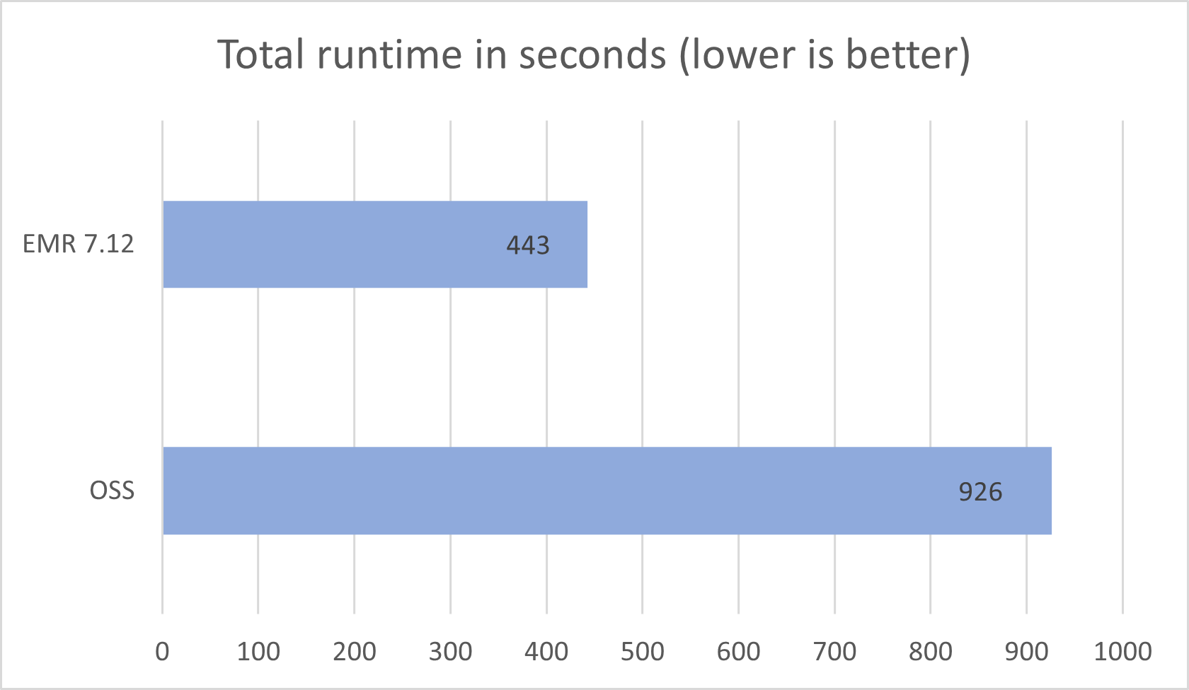
Implement Tenants in your Amazon SES environment, Part 2: Assessment and planning

Post Syndicated from Rommel Sunga original https://aws.amazon.com/blogs/messaging-and-targeting/implement-tenants-in-your-amazon-ses-environment-part-2-assessment-and-planning/

Running multiple users or business units (BUs) on a shared email infrastructure often creates deliverability and compliance risks. The tenant-based reputation isolation feature in Amazon Simple Email Service (Amazon SES) solves these challenges by separating email reputation by customer, BU, or workload. This is part 2 in a series covering the new tenants feature in Amazon Simple Email Service (SES). The first post in this series discussed how users can improve email deliverability with tenant management in Amazon SES (for more details, see the blog post).

In this post, we provide an overview of the tenants feature and guidance for planning the implementation to or migration of your existing Amazon SES infrastructure to use tenant-based reputation isolation.

Part 3 covers practical implementation steps for the tenants feature, including configuration steps for key components like Identity and Access Management (IAM) permissions, Amazon CloudWatch logging, and Amazon EventBridge monitoring. We also provide code examples using the Amazon SES v2 APIs that show how to provision tenants in real time as you onboard downstream customers or business divisions onto your Amazon SES account. Key outcomes include complete reputation isolation between customers, control over sending policies, and automated pause mechanisms for problematic senders.

Solution overview

Amazon SES now offers tenant management capabilities that enable isolated email sending environments within a single AWS account. This provides granular reputation management across different email streams. You can assign dedicated configuration sets, sending identities, and templates to each tenant. Each tenant functions as a logical container that maintains its own sending reputation independently. This tenant-based reputation isolation makes sure deliverability issues with one tenant won’t affect your other tenants. You also get real-time visibility into tenant-level metrics, including messages sent, bounce rates, and complaint rates.

The following diagram illustrates the solution architecture.

Tenants are a best practice for those who want visibility, isolation, and control over their email reputation, from large-scale platforms to smaller teams:

  • Independent software vendors (ISVs) with multiple customers, and marketing and software as a service (SaaS) solutions using a central AWS SES account – You can provision a tenant for each customer to segregate email sending and prevent one client’s sending from negatively affecting deliverability for other clients.
  • Enterprises and other large organizations with multiple BUs – You can maintain separate reputation profiles for different BUs, departments, or brands within the same AWS account.
  • Organizations with distinct mail streams – You can separate transactional and marketing mail, or keep product notifications distinct from internal communications, to make sure issues with one tenant’s email stream don’t affect the other tenants.
  • Single-stream senders – Even if you currently only operate one email stream, you can future-proof your SES account by assigning a tenant from day one. This provides visibility into reputation findings and helps you apply proactive policies to stay ahead of deliverability issues before they impact sending.

In the following sections, we outline how to plan and execute your migration to Amazon SES tenants. We show how to assess your current setup, choose the right tenant structure for your organization, and implement a gradual rollout that minimizes disruption to your existing email operations.

Pre-migration assessment

If you are already using Amazon SES, the transition to tenant-based architecture begins with understanding your current email infrastructure. Start by creating an inventory of your existing sending identities (domains) and identify what, if any, Amazon SES configuration set is assigned. This will help you understand how each customer or BU is currently distributed across your Amazon SES infrastructure. Review each configuration set to identify and track the various configuration options, such as the sending IP pool and archive option. The information you uncover in this phase will serve as the blueprint for your tenant associations and help you make sure each tenant has access to the appropriate resources, while maintaining proper isolation boundaries.

Recommended tenant structure: Individual tenants per customer

For most implementations, we recommend creating one or more tenants per customer or BU so you can achieve complete tenant-level isolation of email workloads. With this approach, you can supply dedicated SMTP or API credentials per tenant to provide secure access to allocated resources. You can apply different reputation policies per tenant as needed and automatically pause any tenant that conflicts with the reputation policy. Additionally, the shared tenant monitoring tools in Amazon SES help you automatically monitor and enforce reputation-based policies at the tenant level, so that problematic email sending behavior from one tenant doesn’t impact the deliverability of others.

The following diagram shows an example of an ISV that operates a SaaS platform on AWS that sends emails on behalf of its many customers from a single Amazon SES account. They have followed the recommended approach by implementing a 1:1 mapping between tenants and customers. This strategy provides complete reputation isolation for each customer and makes sure the ISV operating the Amazon SES account can automatically prevent deliverability issues from one customer from impacting others. This architecture minimizes the reputation damage a single tenant can cause to the ISV’s Amazon SES account’s shared resources like IP pools and domains, making it the optimal choice for maintaining high deliverability standards.

Resource sharing strategies

Your resource allocation strategy depends on your business model and customer segmentation. Consider the following recommended approaches:

  • Complete resource isolation – Each customer, brand, BU, or workload is assigned to individual, dedicated resources using the tenant configuration. This approach offers the simplest migration path: associate each customer’s dedicated resources (identities, IP addresses) with their corresponding tenant and continue operations with enhanced isolation. This model works well for enterprise customers and ISVs who deploy dedicated IPs for customers and require complete separation.
  • Tiered resource sharing – Organizations and ISVs with service tiers (such as free, pro, and VIP) can align tenants and resource sharing with these tiers. Free-tier customers might use the free-tier tenant and share basic resources, pro customers access the pro-tier tenant that maps to enhanced shared resources, and VIP customers receive dedicated resources, often using VIP customer-specific tenants. This balances cost-efficiency with appropriate isolation levels for each customer segment.
  • Extensive resource sharing – Even when email streams share most resources in the Amazon SES account, such as sending identities and IP pools, tenant isolation tenant isolation allows you to protect the sender reputation for independent email streams you send through the shared resources. Consider grouping similar types of customers or email streams into a single tenant or assigning a certain number of customers to each tenant. Although the grouping might be varied, the Amazon SES tenant feature can still minimize the effect of problematic email streams in any one tenant from affecting other tenants by pausing the offending tenant. This helps avoid Amazon SES account-level reputation damage to shared resources, protecting customers and stakeholders using those resources.

Tenant limits and quotas

Amazon SES provides tenant limits to accommodate various organizational scales. The default limit supports 10,000 tenants per account, which is sufficient for most organizations. Qualifying accounts can request increases for more tenants as needed through the Service Quotas console.

Importantly, implementing tenants doesn’t impact your account-level sending quotas or transactions per second (TPS) limits; these remain unchanged and continue to apply across the tenants within your account.

Low-friction adoption

Amazon SES tenants are designed for low-friction adoption, providing isolated containers for your existing Amazon SES email infrastructure. With tenants, you can continue sending emails using your current domains, configuration sets, and IP pools while progressively associating them with appropriate tenants. If you use them, your senders can continue targeting their assigned configuration set. After you’ve configured your Amazon SES account with tenants, instruct your customers or event buses to add a new Amazon SES API call or SMTP header specifying their unique tenant ID. If you aren’t yet using configuration sets, we’ve found that the introduction of the Amazon SES tenants feature often serves as a compelling reason for ISVs and large organizations to adopt configuration sets. If your organization has been looking for ways to offer enhanced email services to existing customers, you might want to use this opportunity to review customer accounts and offer dedicated IPs or email archiving to important email workloads. The ability to gradually roll out the Amazon SES tenants feature facilitates selective adoption, starting with a subset of customers, brands, event buses, or workloads before expanding to your entire customer base. This phased approach enables testing and refinement of your tenant strategy without disrupting existing email operations. Organizations can validate their tenant configuration with low-risk customers before rolling out to critical segments, providing a smooth transition to enhanced reputation management.

Conclusion

In this post, we discussed key aspects of the migration process to Amazon SES tenants, from initial assessment to tenant structure planning. Part 3 of this series will cover details of IAM configuration, monitoring setup, and practical implementation examples. Whether you’re running a SaaS platform, managing multiple brands, operating separate BUs, or just starting to use Amazon SES for your organization, the tenant feature provides simple reputation isolation, boosts efficiency, and helps create better experiences for users.

To learn more, refer to the following resources:


About the authors

Между струните на правилата. Уличните музиканти в София

Post Syndicated from Светла Енчева original https://www.toest.bg/mezhdu-strunite-na-pravilata-ulichnite-muzikanti-v-sofiya/

Между струните на правилата. Уличните музиканти в София

Ако сте ходили из центъра на София, малко вероятно е да не сте ги забелязвали. По „Витошка“, „Графа“, на стълбите и в подлезите на метростанции – уличните музиканти си търсят място там, където минават много хора. Едни излъчват самоувереност, други се притесняват. Някои свирят и пеят добре, други компенсират липсата на умения и талант било с децибели, било с призиви за помощ. 

Как се регулира дейността им? На какви условия трябва да отговарят, за да имат право да свирят на улицата?

Малко предистория и личен опит

През пролетта на 2014 г. написах новина, че на Янко Бреков – Бръснаря, фронтмен на групите „Артерия“ и The Pomorians, не му позволяват да свири на бул. „Витоша“. През онези години беше обичайна практика на уличните музиканти да се казва, че трябва да са с увреждане, за да получат разрешение да упражняват дейността си, макар да нямаше подобно изискване. Новината предизвика медиен интерес; в началото на следващата година темата още не беше заглъхнала. За уличните музиканти обаче нищо не се промени – повечето от тях си останаха все така нарушители.

Тук трябва да призная, че сред тези нарушители съм била и аз – свирила съм веднъж-два пъти с Янко Бръснаря на „Витошка“ (и малко повече в Поморие). Най-ценното от краткия ми опит на това поприще беше общуването с минувачите, които спираха да поприказват, а някои се оказваха музиканти и директно се включваха. Така отнякъде се появи (днес покойният) Явор Захариев от Gravity Co и запя. Дойде и акордеонистът Исус Ангелов с баща си – барабанист, и засвири Smoke on the Water на Deep Purple. От „Витошка“ не са ме гонили, но от крайбрежната алея на Поморие – да.

2025 г.: правила за уличните музиканти в София

Единайсет години по-късно на какви условия трябва да отговарят музикантите, които искат да свирят по софийските улици? Частичен отговор на този въпрос се намира в актуалната Наредба за реда и условията за провеждане на масови мероприятия, опазване на общински имоти и вещи, предназначени за общо ползване и шума в жилищни сгради на територията на Столична община. Чл. 13 от Наредбата постановява:

Ползването на общински имоти и/или имущество, предназначени за общо ползване, за артистична изява се осъществява без използване на озвучителни уредби след издадено разрешение от кмета на района или оправомощено от него длъжностно лице на места определени със заповед от кмета на района. Ползвателят е длъжен да уреди всички отношения, свързани с артистичната изява, за своя сметка.

Обърнах се към общинския съветник от „Спаси София“ Христо Копаранов с молба да разтълкува тези изисквания – освен че е адвокат, има и опит като правозащитник. 

Той уточнява, че последната промяна в наредбата, отнасяща се до музикантите, е добавянето на изречението за уреждането на отношенията, което всъщност се отнася до авторските права. С това изискване, предполагам, Общината си поставя за цел да снеме отговорността за нарушаването на авторското право от себе си. Но представата, че улични артисти ще тръгнат да плащат на големи звукозаписни компании правата за изпълняваните от тях произведения, граничи с абсурда.

По впечатления на Копаранов (а и на всеки, виждал улични музиканти в София), забраната за използване на озвучителни уредби „не се спазва особено“.

Как обаче да се спазва ограничение, което в някои случаи е неприложимо?

Ако някой свири на инструмент, който не е акустичен, без озвучаващо устройство или нищо няма да се чуе (например при MIDI клавиатурите), или звукът ще е далеч от това, което трябва да бъде (например при електрическа китара или бас китара), особено ако се използват ефекти. От друга страна, някои акустични инструменти (например барабани), а и човешки гласове могат да издават по-мощен звук от един портативен усилвател. Вместо да въведе изискване за максимално допустими децибели обаче, Столичният общински съвет просто забранява озвучителите.

Още един практически неизпълним текст от наредбата е чл. 14. Преведен на човешки език, той означава, че е забранено на обществени места да се събират пари, освен от Червения кръст, организации, регистрирани в обществена полза, и вероизповедания. Ако видите уличен музикант, който не събира пари, а свири в студ и пек само за да радва хората с изкуството си, моля да ми кажете – искам да се запозная с този човек.

Според наредбата кметът на Столичната община определя със заповед „реда и условията за издаване на разрешение за изява на улични музиканти, певци и други артисти“.

Тъй като заповедта не може да се намери онлайн, отправям питане в общинската платформа за сигнали има ли такава и ако да, какво съдържа тя. От получения отговор става ясно, че Васил Терзиев е издал въпросната заповед на 31.05.2025 г. В нея се посочва какви точно данни да предоставят изпълнителите на районния кмет, за да им се издаде разрешение, което е със срок между половин и една година. То може да включва различни места за изява, но пък изпълнителите нямат право да се изявяват на едно и също място повече от два часа.

Уличните музиканти – отвъд наредбите и заповедите

Защо има музиканти, които свирят и пеят на улицата, и какво е тяхното отношение към регулацията на дейността им? В рамките на една разходка из центъра на София срещам различни типажи. Някои дори не свирят, а са пуснали силно музика, върху която пеят. Има такива, които са застанали на стълбите на метростанцията, разчитайки не толкова на уменията си, колкото на това, че са (физически) незаобиколим фактор. На „Графа“ жена свири не особено изкусно народна музика на акордеон, но впечатлението, че го прави от нужда, се подсилва от призивите ѝ: „Моля, помогнете!“

Забелязвам и музикантка, за която знам, че работи в операта на областен град. Виждала съм я да свири по софийските улици от двайсетина години. Преди имах впечатлението, че го прави по неволя. Днес обаче изпълнява класически произведения с видимо удоволствие – усмихва се, танцува и увлича хората около себе си.

Сядам да поговоря с един китарист.

Питам го има ли разрешително. Няма. Гонили ли са го полицаите? Да, случвало се е. Няколко пъти е опитвал да си извади разрешително, но не е успял да се дореди:

В началото на всяка година в общината се нарежда една дълга опашка с музиканти, които чакат за разрешение. Местата се запълват, преди да дойде моят ред.

От думите му може да се направи изводът, че съществува нещо като квота за уличните музиканти в района, макар да няма официално обявена информация какъв е максималният им брой. Казва ми, че най-строг е режимът за музикантите в метростанциите – на тях им трябвало не едно разрешително, а две и нямало как да ги пуснат да свирят без тях. Добавя, че стане ли 10 часа вечерта, трябва да престанеш да свириш, дори да имаш разрешително.

На „Витошка“ се запознавам с Никола. Той свири рок на китара, която е свързал с едно портативно усилвателче. От Варна е, живее в София от две години. Питам го защо свири на улицата.

Между струните на правилата. Уличните музиканти в София
Снимка © Светла Енчева

Искам да си вадя хляба с нещо, което обичам. От 15 години свиря на китара. Много исках да отида в музикалното училище, но майка ми беше против.

Натъквам се и на Исус Ангелов.

Той ме помни след запознанството ни преди 11 години на същото място и ме пита още ли свиря на бас. Не, отговарям, обаче съм се върнала към темата за уличните музиканти и искам да взема интервю от него. Исус ме поздравява за идеята и казва, че ще е на мое разположение след половин час на любимото си място – до статуята на Алеко.

Между струните на правилата. Уличните музиканти в София
Снимка © Светла Енчева

Трийсетина минути по-късно се виждаме на уреченото място. Научавам, че Исус има разрешително. Интересувам се какъв е бил редът да си го извади. 

Отивам в общината и свиря пред една комисия, която преценява колко съм добър.

Художествена комисия ли, питам. Отговаря утвърдително. Интересно – нито в наредбата, нито в кметската заповед има информация за художествена комисия.

Разбираемо е, че такава комисия ще даде зелена светлина на Исус – той е може би най-известният музикант в София, ако не и в България, който свири преди всичко на улицата (за разлика от него, Янко Бръснаря става известен с групите си и доста след това започва да свири по софийските и поморийските улици). Участвал е в много концерти, свирил е и в зала 1 на НДК и е единственият самоук музикант, носител на наградата за млади таланти на Фондация „Стоян Камбарев“, която получава през 2025 г.

Исус няма усилвател, защото не му трябва – акордеонът е акустичен инструмент. „Знаеш ли, че човек няма право да свири повече от два часа на едно място?“, обръща ми внимание той, и отбелязва: 

Ако всички спазваха правилата, щеше да е много по-добре!

Решава, че иска да го снимам на видео: „Ще ти изсвиря „Усещане за жена“!“

Изряден уличен музикант – възможно ли е това?

Да обобщим. Един уличен музикант в София трябва, освен да си извади разрешително, да няма усилвател, да се мести на всеки два часа и да не събира никакви пари. Не спазва ли някое от тези изисквания, плюс още куп правила, за някои от които няма лесен начин да научи, от гледна точка на Общината той е просто нарушител на обществения ред.

Дори всички останали условия да са изпълнени, упражняването на попрището без пари изглежда невероятно, дори да си Исус. Шапката или калъфът на музикалния инструмент, където се събират монети, е неразделна част от представата за уличните музиканти. Защото уличното музикантство е труд, а трудът се възнаграждава. Не че е изключено някой да излезе да посвири на хората просто за удоволствие или за да покаже уменията си, но е малко вероятно да го върши безвъзмездно за дълъг период.

Уличните музиканти обаче не са просто нарушители.

Сред тях има такива, които обогатяват градската среда с изкуството си. Освен Исус Ангелов, който става знаменитост, от улицата започва музикалната кариера и на Никола Симеонов – вокалист на популярната група Cool Den. През 2023 г. той организира първия в София фестивал за улична музика.

От улиците на Кьолн започва кариерата и на една от най-известните съвременни германски групи – AnnenMayKantereit. За няколко години тя събира толкова почитатели, че концертите ѝ пълнят стадиони.

Както казва Янко Бръснаря, „улицата е най-трудната сцена“. Единайсет години след като полицаите го гонеха от „Витошка“, свиренето на улицата все още не е съвсем уредено, макар да има известен напредък. Например на музикантите вече не се казва масово, че трябва да са с увреждане, за да получат разрешение. А предложението на Янко за „музикална полиция“ е в известен смисъл осъществено – под формата на художествената комисия, за която споменава Исус.

Уличната музика си прилича с графитите по това, че е трудно да бъде изцяло легална. Както графитите често биват свеждани до вандализъм, така и някои смятат уличните музиканти за нарушители на обществения ред, а песните им – за дразнещ шум. Такава е съдбата на уличното изкуство. Без него обаче градовете биха загубили част от духа си.

How to use the Secrets Store CSI Driver provider Amazon EKS add-on with Secrets Manager

Post Syndicated from Angad Misra original https://aws.amazon.com/blogs/security/how-to-use-the-secrets-store-csi-driver-provider-amazon-eks-add-on-with-secrets-manager/

In this post, we introduce the AWS provider for the Secrets Store CSI Driver, a new AWS Secrets Manager add-on for Amazon Elastic Kubernetes Service (Amazon EKS) that you can use to fetch secrets from Secrets Manager and parameters from AWS Systems Manager Parameter Store and mount them as files in Kubernetes pods. The add-on is straightforward to install and configure, works on Amazon Elastic Compute Cloud (Amazon EC2) instances and hybrid nodes, and includes the latest security updates and bugfixes. It provides a secure and reliable way to retrieve your secrets in Kubernetes workloads.

The AWS provider for the Secrets Store CSI Driver is an open source Kubernetes DaemonSet.

Amazon EKS add-ons provide installation and management of a curated set of add-ons for EKS clusters. You can use these add-ons to help ensure that your EKS clusters are secure and stable and reduce the number of steps required to install, configure, and update add-ons.

Secrets Manager helps you manage, retrieve, and rotate database credentials, application credentials, OAuth tokens, API keys, and other secrets throughout their lifecycles. By using Secrets Manager to store credentials, you can avoid using hard-coded credentials in application source code, helping to avoid unintended or inadvertent access.

New EKS add-on: AWS provider for the Secrets Store CSI Driver

We recommend installing the provider as an Amazon EKS add-on instead of the legacy installation methods (Helm, kubectl) to reduce the amount of time it takes to install and configure the provider. The add-on can be installed in several ways: using eksctl—which you will use in this post—the AWS Management Console, the Amazon EKS API, AWS CloudFormation, or the AWS Command Line Interface (AWS CLI).

Security considerations

The open-source Secrets Store CSI Driver maintained by the Kubernetes community enables mounting secrets as files in Kubernetes clusters. The AWS provider relies on the CSI driver and mounts secrets as file in your EKS clusters. Security best practice recommends caching secrets in memory where possible. If you prefer to adopt the native Kubernetes experience, please follow the steps in this blog post. If you prefer to cache secrets in memory, we recommend using the AWS Secrets Manager Agent.

IAM principals require Secrets Manager permissions to get and describe secrets. If using Systems Manager Parameter Store, principals also require Parameter Store permissions to get parameters. Resource policies on secrets serve as another access control mechanism, and AWS principals must be explicitly granted permissions to access individual secrets if they’re accessing secrets from a different AWS account (see Access AWS Secrets Manager secrets from a different account). The Amazon EKS add-on provides security features including support for using FIPS endpoints. AWS provides a managed IAM policy, AWSSecretsManagerClientReadOnlyAccess, which we recommend using with the EKS add-on.

Solution walkthrough

In the following sections, you’ll create an EKS cluster, create a test secret in Secrets Manager, install the Amazon EKS add-on, and use it to retrieve the test secret and mount it as a file in your cluster.

Prerequisites

  1. AWS credentials, which must be configured in your environment to allow AWS API calls and are required to allow access to Secrets Manager
  2. AWS CLI v2 or higher
  3. Your preferred AWS Region must be available in your environment. Use the following command to set your preferred region:
    aws configure set default.region <preferred_region>
    

  4. The kubectl and eksctl command-line tools
  5. A Kubernetes deployment file hosted in the GitHub repo for the provider

With the prerequisites in place, you’re ready to run the commands in the following steps in your terminal:

Create an EKS cluster

  1. Create a shell variable in your terminal with the name of your cluster:
    CLUSTER_NAME="my-test-cluster”
    

  2. Create an EKS cluster:
    eksctl create cluster $CLUSTER_NAME 
    

eksctl will automatically use a recent version of Kubernetes and create the resources needed for the cluster to function. This command typically takes about 15 minutes to finish setting up the cluster.

Create a test secret

Create a secret named addon_secret in Secrets Manager:

aws secretsmanager create-secret \
  --name addon_secret \
  --secret-string "super secret!"

Set up the Secrets Store CSI Driver provider EKS add-on

Install the Amazon EKS add-on:

eksctl create addon \
  --cluster $CLUSTER_NAME \
  --name aws-secrets-store-csi-driver-provider

Create an IAM role

Create an AWS Identity and Access Management (IAM) role that the EKS Pod Identity service principal can assume and save it in a shell variable (replace <region> with the AWS Region configured in your environment):

ROLE_ARN=$(aws --region <region> --query Role.Arn --output text iam create-role --role-name nginx-deployment-role --assume-role-policy-document '{
    "Version": "2012-10-17",
    "Statement": [
        {
            "Effect": "Allow",
            "Principal": {
                "Service": "pods.eks.amazonaws.com"
            },
            "Action": [
                "sts:AssumeRole",
                "sts:TagSession"
            ]
        }
    ]
}')

Attach a managed policy to the IAM role

Note: AWS provides a managed policy for client-side consumption of secrets through Secrets Manager: AWSSecretsManagerClientReadOnlyAccess. This policy grants access to get and describe secrets for the secrets in your account. If you want to further follow the principle of least privilege, create a custom policy scoped down to only the secrets you want to retrieve.

Attach the managed policy to the IAM role that you just created:

aws iam attach-role-policy \
  --role-name nginx-deployment-role \
  --policy-arn arn:aws:iam::aws:policy/AWSSecretsManagerClientReadOnlyAccess

Set up the EKS Pod Identity Agent

Note: The add-on provides two methods of authentication: IAM roles for service accounts (IRSA) and EKS Pod Identity. In this solution, you’ll use EKS Pod Identity.

  1. After you’ve installed the add-on in your cluster, install the EKS Pod Identity Agent add-on for authentication:
    eksctl create addon \
      --cluster $CLUSTER_NAME \
      --name eks-pod-identity-agent
    

  2. Create an EKS Pod Identity association for the cluster:
    eksctl create podidentityassociation \
        --cluster $CLUSTER_NAME \
        --namespace default \
        --region <region> \
        --service-account-name nginx-pod-identity-deployment-sa \
        --role-arn $ROLE_ARN \
        --create-service-account true
    

Set up your SecretProviderClass

The SecretProviderClass is a YAML file that defines which secrets and parameters to mount as files in your cluster.

  1. Create a minimal SecretProviderClass called spc.yaml for the test secret with the following content:
    apiVersion: secrets-store.csi.x-k8s.io/v1
    kind: SecretProviderClass
    metadata:
      name: nginx-pod-identity-deployment-aws-secrets
    spec:
      provider: aws
      parameters:
        objects: |
          - objectName: "addon_secret"
            objectType: "secretsmanager"
        usePodIdentity: "true"
    

  2. Deploy your SecretProviderClass (make sure you’re in the same directory as the spc.yaml you just created):
    kubectl apply -f spc.yaml
    

To learn more about the SecretProviderClass, see the GitHub readme for the provider.

Deploy your pod to your EKS cluster

For brevity, we’ve omitted the content of the Kubernetes deployment file. The following is an example deployment file for Pod Identity in the GitHub repository for the provider—use this file to deploy your pod:

kubectl apply -f https://raw.githubusercontent.com/aws/secrets-store-csi-driver-provider-aws/main/examples/ExampleDeployment-PodIdentity.yaml

This will mount addon_secret at /mnt/secrets-store in your cluster.

Retrieve your secret

  1. Print the value of addon_secret to confirm that the secret was mounted successfully:
    kubectl exec -it $(kubectl get pods | awk '/nginx-pod-identity-deployment/{print $1}' | head -1) -- cat /mnt/secrets-store/addon_secret
    

  2. You should see the following output:
    super secret!
    

You’ve successfully fetched your test secret from Secrets Manager using the new Amazon EKS add-on and mounted it as a file in your Kubernetes cluster.

Clean up

Run the following commands to clean up the resources that you created in this tutorial:

aws secretsmanager delete-secret \
  --secret-id addon_secret \
  --force-delete-without-recovery

aws iam delete-role --role-name nginx-deployment-role

eksctl delete cluster $CLUSTER_NAME

Conclusion

In this post, you learned how to use the new Amazon EKS add-on for the AWS Secrets Store CSI Driver provider to securely retrieve your secrets and parameters and mount them as files in your Kubernetes clusters. The new EKS add-on provides benefits such as the latest security patches and bug fixes, tighter integration with Amazon EKS, and reduces the time it takes to install and configure the AWS Secrets Store CSI Driver provider. The add-on is validated by EKS to work with EC2 instances and hybrid nodes.

Further reading

If you have feedback about this post, submit comments in the Comments section below. If you have questions about this post, contact AWS Support.

Angad Misra

Angad Misra

Angad is a Software Engineer on the AWS Secrets Manager team. When he isn’t building secure, reliable, and scalable software from first principles, he enjoys a good latte, live music, playing guitar, exploring the great outdoors, cooking, and lazing around with his cat, Freyja.

KDE Plasma 6.8 will be Wayland-only

Post Syndicated from jzb original https://lwn.net/Articles/1048208/

KDE’s Plasma team has announced
that KDE Plasma will drop X11 session support with Plasma 6.8:

The Plasma X11 session will be supported by KDE into early
2027.

We cannot provide a specific date, as we’re exploring the
possibility of shipping some extra bug-fix releases for Plasma
6.7. The exact timing of the last one will only be known when we get
closer to its actual release, which we expect will be sometime in
early 2027.

What if I still really need X11?

This is a perfect use case for long term support (LTS)
distributions shipping older versions of Plasma. For example,
AlmaLinux 9 includes the Plasma X11 session and will be supported
until sometime in 2032.

See the blog post for information on running X11 applications
(still supported), accessibility, gaming, and more.

Secure Amazon Elastic VMware Service (Amazon EVS) with AWS Network Firewall

Post Syndicated from Sheng Chen original https://aws.amazon.com/blogs/architecture/secure-amazon-elastic-vmware-service-amazon-evs-with-aws-network-firewall/

Amazon Elastic VMware Service (Amazon EVS) helps organizations migrate, run, and scale VMware workloads natively on AWS. It delivers a VMware Cloud Foundation (VCF) environment that operates directly within your Amazon Virtual Private Cloud (Amazon VPC) on Amazon EC2 bare-metal instances. The solution helps customers accelerate cloud migrations and data center exits without needing to refactor existing applications.

For customers considering a hybrid cloud architecture, a unified network security solution is required to protect application traffic across Amazon EVS environments, Amazon VPCs, on-premises data centers and the internet. It also needs to provide a single point of control for firewall policy management, centralized logging, and monitoring to streamline network security operations.

AWS Network Firewall is a managed firewall and intrusion detection and prevention service (IDS/IPS) that can help address these requirements. Built on AWS managed infrastructure, it automatically scales with traffic demands while maintaining high availability and consistent performance. The service provides centralized policy management and traffic inspection across multiple VPCs and AWS accounts. Additionally, it provides comprehensive visibility and reporting through firewall log collections to Amazon Simple Storage Service (Amazon S3), Amazon CloudWatch Logs, or Amazon Data Firehose.

In this post, we demonstrate how to utilize AWS Network Firewall to secure an Amazon EVS environment, using a centralized inspection architecture across an EVS cluster, VPCs, on-premises data centers and the internet. We walk through the implementation steps to deploy this architecture using AWS Network Firewall and AWS Transit Gateway.

Architecture overview

AWS Network Firewall operates as a “bump-in-the-wire” solution, which transparently inspects and filters network traffic across Amazon VPCs. It is inserted directly into the traffic path by updating VPC or Transit Gateway route tables, allowing it to examine all packets without requiring any changes to the existing application flow patterns.

The following diagram depicts the architecture overview of our centralized inspection model using AWS Network Firewall.

Figure 1: Secure Amazon EVS with AWS Network Firewall using centralized inspection architecture

Figure 1: Secure Amazon EVS with AWS Network Firewall using centralized inspection architecture

The Amazon EVS environment is deployed directly within a customer VPC (i.e. EVS VPC), which consists of EVS VLAN subnets that form the underlay networks for VCF deployment. This infrastructure provides connectivity for NSX overlay networks, host management, vMotion, and vSAN. Amazon VPC Route Server enables dynamic routing between the underlay networks and overlay networks. For more information, see Concepts and components of Amazon EVS.

The architecture also includes a standard workload VPC (i.e. VPC01), and a Direct Connect Gateway connects to the on-premises data center via an AWS Direct Connect connection. We use a dedicated egress VPC with NAT gateways for centralized internet egress, and a separate ingress VPC with Application Load Balancers to terminate ingress web traffic and steer flows back to the target services.

With this architecture, the following traffic flow patterns can be inspected:

East-West Traffic:

  • Between EVS VPCs and Workload VPCs
  • Between Workload VPCs

North-South Traffic:

  • Between EVS/Workload VPCs and on-premises
  • Between EVS/Workload VPCs and internet
  • Between on-premises and internet

The centralized inspection architecture provides several benefits:

  • Single point of control for network security inspection across multiple VPCs
  • Enhanced rule enforcement across AWS infrastructure, on-premises resources, and the internet
  • Centralized logging and monitoring

For this demo we use the AWS Network Firewall native integration with AWS Transit Gateway capability to streamline firewall deployment and management. With a native firewall attachment, AWS automatically provisions and manages all the necessary VPC resources, reducing the operational overhead of managing subnets, route tables, and firewall endpoints within the inspection VPC.

Prerequisites

This post assumes familiarity with: AWS Command Line Interface (AWS CLI), Amazon VPC, Amazon EC2, NAT gateway, Application Load Balancer, Internet gateway, AWS Direct Connect, AWS Transit Gateway and the VMware VCF platform.

The following prerequisites are necessary to complete this solution.

  • An EVS VPC includes:
    • An Amazon EVS cluster (minimum 4x i4i nodes)
    • VPC CIDR: 10.0.0.0/16
    • NSX Segments CIDR: 192.168.0.0/19 (summarized)
    • A VPC Route Server deployed in the EVS VPC to receive NSX segment routes via BGP dynamic routing. Refer to the EVS User Guide for more details.
  • A Workload VPC (VPC01):
    • CIDR: 172.21.0.0/16
  • An Egress VPC:
    • CIDR: 172.23.0.0/16
    • 1x Internet Gateway
    • 1x NAT Gateway
  • An Ingress VPC:
    • CIDR: 172.24.0.0/16
    • 1x Internet Gateway
    • 1x Application Load Balancer
  • Optional: a Direct Connect Gateway:
    •  connecting to the on-premises environment (10.0.0.0/8)

Note: The CIDR blocks used in this example are for demo purposes only; change the address spaces to match your own networking environment. The design can also be scaled to include additional EVS environments and/or other VPCs based on workload needs.

Walkthrough

In this section, we walk through the implementation steps to deploy the centralized inspection architecture with AWS Network Firewall and AWS Transit Gateway. We focus on the overall network integration of the architecture without diving into the detailed configurations of AWS Network Firewall or Transit Gateway.

1. Create an AWS Transit Gateway

In the VPC console, create a Transit Gateway. Make sure to deselect the following options:

  • Default route table association
  • Default route table propagation

Create two empty transit gateway route tables and associate them with the Transit Gateway.

  • Pre-inspection route table: steers traffic into the AWS Network Firewall for centralized inspection
  • Post-inspection route table: returns traffic back to its original destination after inspection and is permitted by the AWS Network Firewall

2. Attach VPCs to the Transit Gateway

Attach all four VPCs (EVS, VPC01, Ingress, Egress) to the same Transit Gateway. The Direct Connect Gateway can also be attached to the Transit Gateway if AWS Network Firewall is needed to inspect traffic between the on-premises environment and AWS or the internet.

Figure 2: Attach VPCs to the Transit Gateway

Figure 2: Attach VPCs to the Transit Gateway

Associate all attachments to the pre-inspection Transit Gateway route table.

Figure 3: Associate VPC attachments to the pre-inspection route table

Figure 3: Associate VPC attachments to the pre-inspection route table

3. Create an AWS Network Firewall with Transit Gateway native integration

In the Network Firewall section of the VPC console, choose Create firewall.

At the Attachment type section, select Transit Gateway to enable native integration with the existing Transit Gateway.

Figure 4: Enable AWS Network Firewall native integration with Transit Gateway

Figure 4: Enable AWS Network Firewall native integration with Transit Gateway

At the Logging configuration, enable the following log types with CloudWatch log group as the log destination. Create a log group for each log type in the CloudWatch Console.

  • Alert: /anfw-centralized/anfw01/alert
  • Flow: /anfw-centralized/anfw01/flow

Create and associate an empty firewall policy to deploy the AWS Network Firewall instance. The firewall policy contains a list of rule groups that define how the firewall inspects and manages traffic. This empty firewall policy can be configured later.

With the Transit Gateway native integration enabled, a Transit Gateway attachment is automatically created for the AWS Network Firewall, with the resource type shown as Network Function. In addition, the Appliance Mode is automatically enabled for the firewall attachment to make sure the Transit Gateway continues to use the same Availability Zone (AZ) for the attachment over the lifetime of a flow.

Associate the firewall attachment to the post-inspection Transit Gateway route table.

Figure 5: AWS Network Firewall native attachment

Figure 5: AWS Network Firewall native attachment

4. Update Transit Gateway route tables

Update the pre-inspection Transit Gateway route table with a default route that points to the AWS Network Firewall attachment. This makes sure traffic that arrives to the Transit Gateway from all VPC attachments and the Direct Connect Gateway attachment is sent to the firewall for centralized inspection.

Figure 6: Transit Gateway pre-inspection route table

Figure 6: Transit Gateway pre-inspection route table

Add the following static routes to the post-inspection route table to direct return traffic back to each VPC and the Direct Connect Gateway accordingly.

Figure 7: Transit Gateway post-inspection route table

Figure 7: Transit Gateway post-inspection route table

5. Update VPC route tables

Finally, update route tables at each VPC as per the following table.

Make sure to add the following routes at the relevant VPC route tables:

  • EVS VPC and VPC01 have a default route (marked in blue) to steer all egress flows into AWS Network Firewall for centralized inspection.
  • Ingress VPC and Egress VPC have RFC-1918 routes (marked in green) to direct return traffic to the Transit Gateway.

Within the EVS VPC, notice the NSX segment routes are automatically propagated to the NSX uplink subnet route table and the private subnet route table via the VPC Route Server.

Figure 8: NSX uplink subnet route table within EVS VPC

Figure 8: NSX uplink subnet route table within EVS VPC

A centralized security inspection architecture has now been deployed for the EVS environment, using AWS Network Firewall with Transit Gateway native integration.

6. Testing

Egress inspection (FQDN filtering)

To test egress inspection from EVS VPC or VPC01 to the internet, create a stateful rule group for the firewall instance using FQDN filtering:

  • Rule group format: Domain list
  • Domain names: .google.com
  • Source IPs: 192.168.0.0/19, 172.21.0.0/16
  • Protocols: HTTP & HTTPS
  • Action: Allow

As expected, testing web access from a virtual machine (192.168.12.10) within the EVS environment to the allowed domain (i.e. google.com) is permitted by the AWS Network Firewall. However, access to unauthorized domain (i.e. facebook.com) is blocked at the firewall with an alert trigged, which can be verified at the CloudWatch log group at /aws/network-firewall/alert/.

Figure 9: Egress inspection from EVS to internet with FQDN filtering

Figure 9: Egress inspection from EVS to internet with FQDN filtering

Ingress inspection

Create another stateful rule group to allow Application Load Balancers deployed within the Ingress VPC to access a web server running in the EVS environment via HTTP protocol:

  • Rule group format: Standard stateful rule
  • Geographic IP Filtering: Disable Geographic IP filtering
  • Protocol: HTTP
  • Source: 172.24.0.0/16
  • Source Port: ANY
  • Destination: 192.168.12.10/32
  • Destination Port ANY
  • Traffic direction: Forward
  • Action: Alert

The CloudWatch firewall logs show an Application Load Balancer (172.24.6.45) from the Ingress VPC can establish HTTP connection to the EVS web server (192.168.12.10). Additionally, the Application Load Balancer has successfully registered the EVS web server as a remote IP target.

Figure 10: Ingress inspection from Ingress VPC to EVS

Figure 10: Ingress inspection from Ingress VPC to EVS

East-West inspection

For East-West inspection testing, update the previous stateful rule group to add a new rule to block ICMP traffic from VPC01 to the EVS VPC.

  • Rule group format: Standard stateful rule
  • Geographic IP Filtering: Disable Geographic IP filtering
  • Protocol: ICMP
  • Source: 172.21.0.0/16
  • Source Port: ANY
  • Destination: 192.168.0.0/19
  • Destination Port: ANY
  • Action: Drop

As a result, pings from an EC2 instance (172.21.128.4) from VPC01 to the EVS web server (192.168.12.10) are being dropped.

Figure 11: East-West Inspection from VPC01 to EVS

Figure 11: East-West Inspection from VPC01 to EVS

Conclusion

In this post, we demonstrated how to utilize AWS Network Firewall to secure Amazon EVS workloads and to provide centralized traffic inspection between Amazon EVS environments, Amazon VPCs, on-premises data centers, and the internet. We walked through the implementation steps for deploying the centralized inspection architecture using AWS Network Firewall and AWS Transit Gateway.

To learn more, review these resources:


About the authors

Amazon Route 53 launches Accelerated recovery for managing public DNS records

Post Syndicated from Micah Walter original https://aws.amazon.com/blogs/aws/amazon-route-53-launches-accelerated-recovery-for-managing-public-dns-records/

Today, we’re announcing Amazon Route 53 Accelerated recovery for managing public DNS records, a new Domain Name Service (DNS) business continuity feature that is designed to provide a 60-minute recovery time objective (RTO) during service disruptions in the US East (N. Virginia) AWS Region. This enhancement ensures that customers can continue making DNS changes and provisioning infrastructure even during regional outages, providing greater predictability and resilience for mission-critical applications.

Customers running applications that require business continuity have told us they need additional DNS resilience capabilities to meet their business continuity requirements and regulatory compliance obligations. While AWS maintains exceptional availability across our global infrastructure, organizations in regulated industries like banking, FinTech, and SaaS want the confidence that they will be able to make DNS changes even during unexpected regional disruptions, allowing them to quickly provision standby cloud resources or redirect traffic when needed.

Accelerated recovery for managing public DNS records addresses this need by targeting DNS changes that customers can make within 60 minutes of a service disruption in the US East (N. Virginia) Region. The feature works seamlessly with your existing Route 53 setup, providing access to key Route 53 API operations during failover scenarios, including ChangeResourceRecordSets, GetChange, ListHostedZones, and ListResourceRecordSets. Customers can continue using their existing Route 53 API endpoint without modifying applications or scripts.

Let’s try it out
Configuring a Route53 hosted zone to use accelerated recovery is simple. Here I am creating a new hosted zone for a new website I’m building.

Once I have created my hosted zone, I see a new tab labeled Accelerated recovery. I can see here that accelerated recovery is disabled by default.

To enable it, I just need to click the Enable button and confirm my choice in the modal that appears as depicted in the dialog below.

Enabling accelerated recovery will take a couple minutes to complete. Once it’s enabled, I see a green Enabled status as depicted in the screenshot below.

I can disable accelerated recovery at any time from this same area of the AWS Management Console. I can also enable accelerated recovery for any existing hosted zones I have already created.

Enhanced DNS business continuity
With accelerated recovery enabled, customers gain several key capabilities during service disruptions. The feature maintains access to essential Route 53 API operations, ensuring that DNS management remains available when it’s needed most. Organizations can continue to make critical DNS changes, provision new infrastructure, and redirect traffic flows without waiting for full service restoration.

The implementation is designed for simplicity and reliability. Customers don’t need to learn new APIs or modify existing automation scripts. The same Route 53 endpoints and API calls continue to work, providing a seamless experience during both normal operations and failover scenarios.

Now available
Accelerated recovery for Amazon Route 53 public hosted zones is available now. You can enable this feature through the AWS Management Console, AWS Command Line Interface (AWS CLI), AWS Software Development Kit (AWS SDKs), or infrastructure as code tools like AWS CloudFormation and AWS Cloud Development Kit (AWS CDK). There is no additional cost for using accelerated recovery.

To learn more about accelerated recovery and get started, visit the documentation. This new capability represents our continued commitment to providing customers with the DNS resilience they need to build and operate mission-critical applications in the cloud.

The collective thoughts of the interwebz