Code, confidence, and community: A look back at Astro Pi 2024–25

Post Syndicated from Fergus Kirkpatrick original https://www.raspberrypi.org/blog/code-confidence-and-community-a-look-back-at-astro-pi-2024-25/

Taking part in the European Astro Pi Challenge builds young people’s confidence and motivates them to try further digital making and programming activities, according to their mentors. The challenge, a European Space Agency (ESA) Education project run in collaboration with the Raspberry Pi Foundation, offers young people the amazing opportunity to write a short computer program to run on Raspberry Pi computers on board the International Space Station (ISS).

An incredible 27,304 young people from 27 countries got involved in Astro Pi 2024–25, with 26,294 succeeding in having their code run in space across the two challenge activities, Mission Zero and Mission Space Lab. As in past years, we’ve asked mentors and their teams about their experience and the impact participating had on them. So what did they say?

How we listened to feedback

To find out what worked well, what we could improve, and the impact Astro Pi has had on young people’s lives this year, we encouraged mentors to complete a survey after teams submitted their computer programs. We also ran focus group discussions to deepen our understanding. A huge thank you to the 99 Mission Zero and 26 Mission Space Lab mentors who completed our surveys, and the five mentors who participated in our focus groups.

A selection of earth observation images captured by MSL teams.
A selection of earth observation images captured by MSL teams

What is working well

Low stakes but high impact

Mentors believe that Astro Pi is a great opportunity for young people to build their coding skills and knowledge of STEM concepts. Close to 80% of mentors for Mission Zero and 90% for Mission Space Lab agreed that these outcomes were being achieved for the young people in their teams. Mentors also appreciated that while the programme had real-world application, the learning experience was relaxed and low pressure.

Many of our young participants come from areas of educational disadvantage or traditionally underrepresented groups where confidence with technology and STEM subjects can be low. Mentors reported that the programme empowers young people, increasing their confidence with computing and digital making, and helping them connect with a wider community of learners from around the world. 

“They [young people] come from complicated environments and sometimes their confidence is very low. They don’t believe in themselves and this [Mission Zero challenge] really empowers them.” — Mission Zero mentor

“I think having a space mission, having Mission Zero is a way of connecting not only to a worldwide group of learners, but also explorers, future scientists, future astronauts. To see them as part of a larger community, not just an activity or assignment that they have to do in class. They discover their own abilities and potential, and exercise their creativity in a very low stakes environment… and then to see it come to life in that global way I think is extremely valuable.” — Mission Zero mentor

This increased confidence also encourages young people to take on other opportunities. 78% of Mission Zero mentors and 96% of Mission Space Lab mentors believe that it is likely that their students will participate in other coding and digital making challenges in the future. 

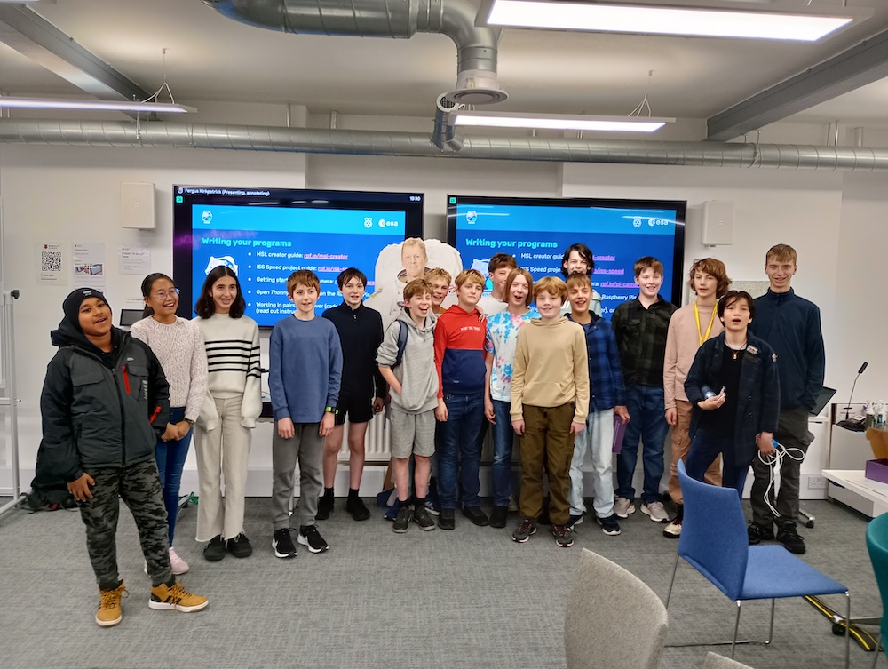
A group of students at a Mission Space Lab hackathon event.
A group of students at a Mission Space Lab hackathon event

Space is cool!

The connection to space and the ISS continues to be a strong motivator, not just for young people but also mentors and other peers. In our survey, 90% of mentors in Mission Zero and 92% in Mission Space Lab reported that the young people participating were highly motivated by the possibility of having their code run on the ISS. In focus groups, mentors highlighted how the excitement of working on a space project extended to them and other adults too.

“They’ve always really enjoyed the sheer fact that you get to send stuff into space because it is really cool.” — Mission Zero mentor

“You know, even the adults I tell about this say, ‘oh, that sounds amazing. Can I do it?’ I go, ‘No, you’re too old. I’m too old.’” — Mission Zero mentor

“We want our code to run in space! We are fascinated by discovery and the opportunity to contribute to a real science experiment on the ISS.” — Mission Space Lab mentor

The resources and guidance are useful

We know how crucial mentors are to the success of Astro Pi. Mentors come from diverse backgrounds and we are committed to making sure they feel prepared and supported. We were thrilled to hear that over 90% of Mission Zero mentors and 80% of Mission Space Lab mentors found the Astro Pi resources useful.

“I had no skills but the support proved to be excellent” — Mission Zero mentor

“Step-by-step instructions were excellent and really clear. Very easy to follow.” — Mission Zero mentor

For Mission Space Lab, the more technical activity, we’ve been working on providing additional support. In 2024–25 we introduced a new online simulator tool for teams to test their programs with historical ISS data. Mentors found the tool to be helpful, allowing them to troubleshoot their code.

An illustration of the ISS sending files back to a satellite on Earth.
An illustration of the ISS sending files back to a satellite on Earth

What could be improved?

While we celebrate the successes, we’re always keen to understand how we can improve the programme.

As in previous years, mentors reported that young people whose computer programs passed the eligibility criteria and ran on the ISS (or “achieved flight status”, as we call it) benefited most from the experience. While 12% more Mission Space Lab teams achieved flight status this year compared to last year, some registered teams still did not submit programs. 

To understand why, we surveyed mentors who had registered but who did not then submit computer programs. In the 55 responses, the main reasons given were a shortage of time due to other school commitments, and their teams finding the challenge difficult. 

Some survey respondents suggested a need for more simplified, step-by-step instructions for less experienced learners. Additionally, a few teams faced technical issues with the online portal and the testing tool.

Thank you to all the mentors who provided their honest feedback. We’ve read and considered all of it and will use it to make Astro Pi even better in the future.

Astro Pi will be launching for its 10th year on Monday, 8 September 2025. We’ve been working on making it easier than ever to take part in both missions and are looking forward to supporting you and your teams in getting your code into space. If you’re interested in taking part, sign up to our newsletter and get the latest news and information about our resources for this year’s missions. 

Important dates:

8 September 2025: The Astro Pi Challenge opens for registration

16 February 2026: Closing date for Mission Space Lab

23 March 2026: Closing date for Mission Zero

The post Code, confidence, and community: A look back at Astro Pi 2024–25 appeared first on Raspberry Pi Foundation.

Jim Sanborn Is Auctioning Off the Solution to Part Four of the Kryptos Sculpture

Post Syndicated from Bruce Schneier original https://www.schneier.com/blog/archives/2025/08/jim-sanborn-is-auctioning-off-the-solution-to-part-four-of-the-kryptos-sculpture.html

Well, this is interesting:

The auction, which will include other items related to cryptology, will be held Nov. 20. RR Auction, the company arranging the sale, estimates a winning bid between $300,000 and $500,000.

Along with the original handwritten plain text of K4 and other papers related to the coding, Mr. Sanborn will also be providing a 12-by-18-inch copper plate that has three lines of alphabetic characters cut through with a jigsaw, which he calls “my proof-of-concept piece” and which he kept on a table for inspiration during the two years he and helpers hand-cut the letters for the project. The process was grueling, exacting and nerve wracking. “You could not make any mistake with 1,800 letters,” he said. “It could not be repaired.”

Mr. Sanborn’s ideal winning bidder is someone who will hold on to that secret. He also hopes that person is willing to take over the system of verifying possible solutions and reviewing those unending emails, possibly through an automated system.

Here’s the auction listing.

Zeta reduces banking incident response time by 80% with Amazon OpenSearch Service observability

Post Syndicated from Deepesh Dhapola original https://aws.amazon.com/blogs/big-data/zeta-reduces-banking-incident-response-time-by-80-with-amazon-opensearch-service-observability/

This is a guest post co-written with Shashidhar Soppin, Manochandra Menni and Anchal Kansal from Zeta.

Zeta is a core banking technology provider that enables banks to rapidly launch extensible banking assets and liability products. Zeta’s primary products are Olympus and Tachyon. Olympus is a platform as a service (PaaS) that simplifies building and operating cloud-native, secure and distributed multi-tenant software as a service (SaaS) products. It blends infrastructure as code and GitOps methodologies for efficient and consistent deployment of SaaS products. Its architecture prioritizes strong tenant isolation, real-time event processing, and comprehensive observability, supporting robust API integrations and seamless deployment. Zeta’s Tachyon is a full-stack, cloud-native, API-first digital-banking SaaS service delivered via Olympus. The banking services of Tachyon include payment engines (for UPI, credit, debit, and prepaid cards), savings & checking account management, etc. Tachyon is a modern debit processing product with personal finance management and card controls. It is designed to increase usage, upsell credit, reduce fraud, and improve customer satisfaction. The Tachyon product offers comprehensive provisioning, payments, and account management APIs and SDKs, enabling seamless integration of financial products into third-party apps without compromising privacy and security. Zeta operates Tachyon as a multi-tenant SaaS product, serving customers who are configured as individual tenants within the system. Zeta’s technology stack is monitored by their Customer Service Navigator product (CSN), which is part of Olympus.

As a global SaaS provider, Zeta needed a solution capable of monitoring tenants, measuring SLAs, meeting local regulatory requirements, and scaling efficiently with both new tenant onboarding and seasonal usage spikes. Zeta sought a cost-effective, scalable system that would provide a unified “single pane of glass” to monitor the application services, cloud infrastructure, open-source components, and third-party products.

Zeta faced a formidable challenge in orchestrating a cohesive monitoring system across a rapidly expanding multi-tenant environment, diverse domains, and numerous tools. As more tenants joined their system, the complexity grew exponentially, making Zeta’s monitoring solution increasingly difficult to maintain. The primary challenge stemmed from fragmented monitoring tools that made it difficult to quickly identify root causes across interconnected systems, leading to prolonged troubleshooting times and potential service degradation. When users reported issues, such as credit card payment problems, Site Reliability Engineering (SRE) team had to navigate through a several disparate monitoring tools and siloed data, and the lack of integrated observability resulted in time-consuming manual correlation efforts. This multi-tenant, multi-solution landscape significantly complicated the ability to maintain consistent monitoring standards and service levels. The challenge was further complicated by the complex regulatory landscape, where global expansion required adherence to diverse local regulations, necessitating a flexible architecture capable of accommodating varying data retention policies and access controls across different jurisdictions. Each new tenant addition multiplied the complexity of balancing the monitoring needs of internal SRE teams and customers, requiring sophisticated data segregation and access management. Additionally, Zeta required comprehensive anomaly detection capabilities across systems, components, infrastructure, and operations, requiring a solution that could scale dynamically while establishing dynamic baselines and identifying subtle patterns that might indicate emerging issues. As the tenant base continued to grow, the need for a unified, scalable monitoring solution that could streamline these processes, enhance operational visibility, and maintain system integrity became critical.

Zeta’s goal was to streamline their processes and enhance operational visibility across the entire technology landscape. By addressing these challenges, Zeta aimed to create a unified observability solution that would significantly improve incident response times, enhance regulatory compliance posture, and ultimately deliver a more reliable and performant service to their global customer base.

In this post we explain how Zeta built a more unified monitoring solution using Amazon OpenSearch Service that improved performance, reduced manual processes, and increased end-user satisfaction. Zeta has achieved over an 80% reduction in mean time to resolution (MTTR), with incident response times decreasing from 30+ minutes to under 5 minutes.

Solution overview

Zeta designed and built an observability system, CSN, to deliver comprehensive visibility across the service environment. CSN is part of the Olympus suite of products. CSN serves as the primary interface for the SRE team, offering real-time service health dashboards, infrastructure monitoring, SLA performance analytics, and an admin panel for user management. The system is equipped with single sign-on (SSO) integration and enforces role-based access control (RBAC) to enable secure, granular access. With CSN, SREs can efficiently monitor system health, receive actionable alerts and warnings, and manage operational workflows across critical services.

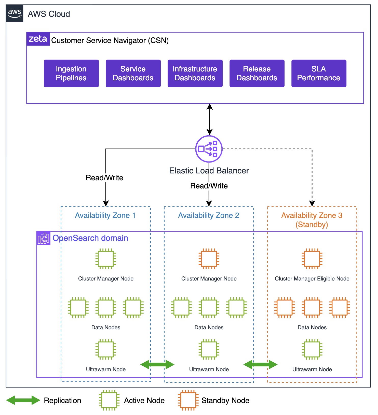
CSN is powered by OpenSearch Service to provide an integrated solution for DevOps and Site Reliability Engineers to help identify critical events and issues. Zeta chose OpenSearch Service because it offers a fully managed, open-source search analytics engine that scales effortlessly to handle the increasing number of tenants, associated data growth, and analytics needs. It’s seamless integration with AWS services, robust security features, and support for real-time data ingestion and querying make it ideal for powering the CSN dashboards and analytics workloads. The following diagram illustrates the CSN deployment architecture.

Zeta CSN Deployment Architecture

The OpenSearch Service domain uses the Multi-AZ with Standby deployment model, following AWS best practices for high availability and fault tolerance. Nodes—including dedicated cluster manager nodes, data nodes, and UltraWarm nodes—are distributed evenly across three Availability Zones in the same AWS Region. Availability Zones 1 and 2 handle active indexing and search traffic, and Availability Zone 3 contains standby nodes that remain passive during normal operations. If an Availability Zone failure occurs, OpenSearch Service automatically promotes standby nodes to active status, maintaining cluster operations with minimal disruption and no need for data redistribution.

The OpenSearch cluster consists of three dedicated cluster manager nodes and a multiple-of-three data node count to maintain quorum and balanced shard allocation. Each index uses at least two replicas, providing redundant copies of data across the Availability Zones. This Multi-AZ with Standby configuration delivers high resilience and rapid failover, supporting continuous service availability and robust disaster recovery for the observability workloads.

Data collection and ingestion

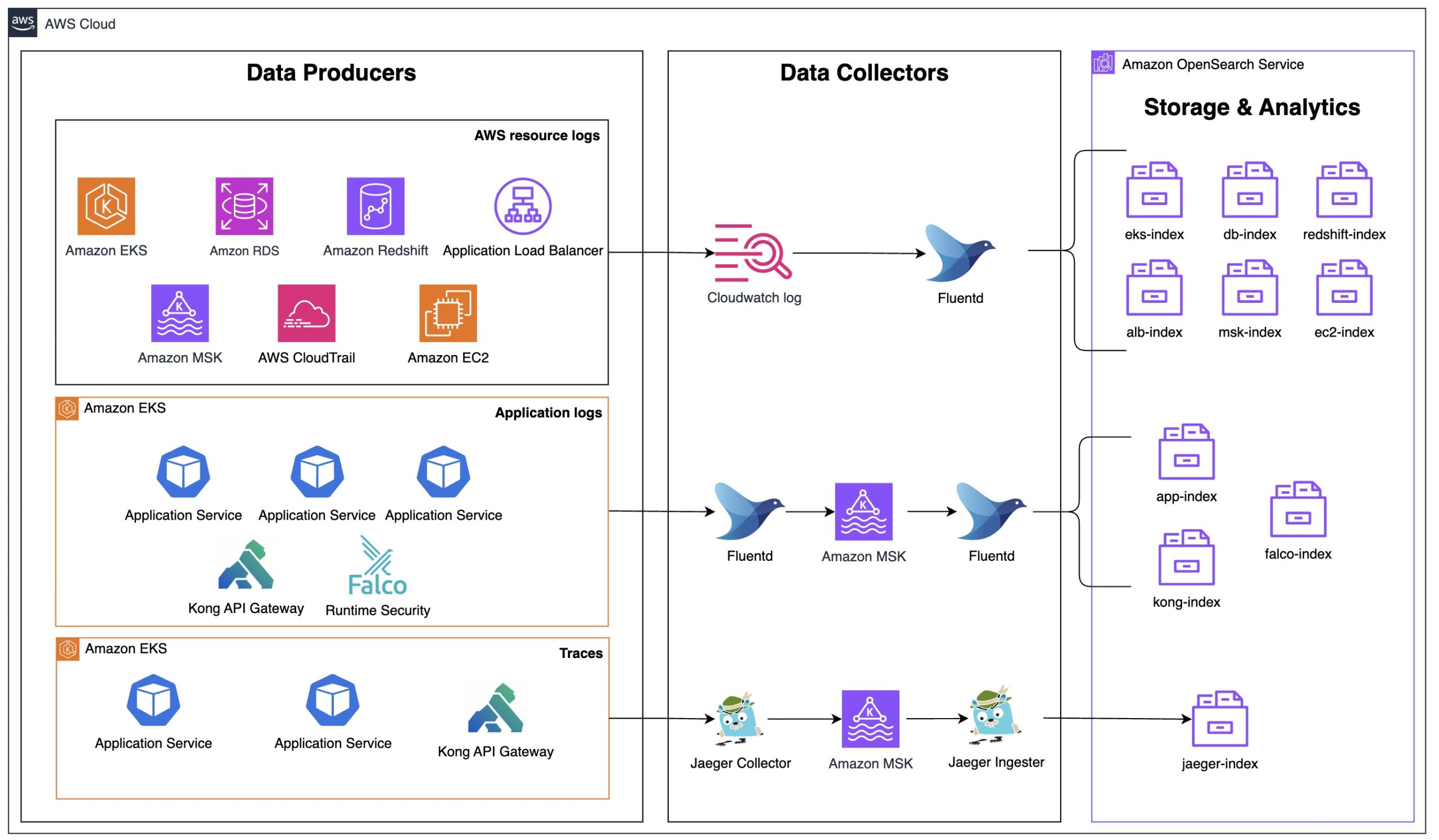
The observability strategy centers on a data collection and ingestion pipeline designed to handle the complexity and scale. The architecture, as shown in the following diagram, addresses three critical data types: AWS resource logs, application logs, and distributed traces, with each data type using tailored collection and processing methods optimized for the workloads.

Zeta CSN Data Ingestion

AWS resource logs collection

The infrastructure spans multiple AWS services including Amazon Elastic Kubernetes Service(Amazon EKS), Amazon Relational Database Service(Amazon RDS), Amazon Redshift, Application Load Balancer, Amazon Managed Streaming for Apache Kafka (Amazon MSK), Amazon Elastic Compute Cloud (Amazon EC2) and more. Zeta uses Amazon CloudWatch Logs as the primary collection point for AWS service logs, which provides native integration with these services.

AWS services send their logs directly to CloudWatch Logs, which are then pulled by Fluentd running on the Amazon EKS cluster for centralized processing. This approach natively captures operational data from the AWS resources, including:

  • Database operational logs and audit trails from Amazon RDS instances
  • Data warehouse query execution logs from Amazon Redshift
  • Application Load Balancer access logs capturing traffic patterns and performance metrics
  • Kafka cluster operational logs from Amazon MSK
  • AWS API invocation audit trails from AWS CloudTrail
  • Container runtime and operating system logs from Amazon EC2
  • During the log collection, personally identifiable information (PII) is filtered out. The solution adheres strictly to PCI-DSS guidelines throughout this process.

Zeta used Amazon MSK as a scalable and reliable backbone for collecting and streaming logs from various sources across the AWS resources. Logs are ingested into Amazon MSK, providing a durable and fault-tolerant buffer that decouples log producers from consumers. This architecture enables real-time log streaming and supports advanced processing pipelines before the logs are routed to the OpenSearch Service. By integrating Amazon MSK into the logging workflow, scalability, resilience, and flexibility is improved, so that high log volumes are efficiently managed without impacting downstream systems. This approach, combined with native AWS integrations, minimizes operational complexity and maintains comprehensive, centralized log visibility across the cloud environment.

Fluentd processes these logs and routes them directly to OpenSearch Service, maintaining the benefits of AWS integration while providing centralized accessibility. This centralized logging approach with built-in buffering capabilities reduces the direct load on OpenSearch Service by batching and optimizing log delivery, helping to prevent potential ingestion bottlenecks during high-volume periods. The approach alleviates the need for custom log shipping agents on AWS resources, reducing operational overhead while maintaining comprehensive coverage of the cloud infrastructure.

Application logs processing

For application-level observability, a pipeline using Fluentd is deployed as Kubernetes DaemonSet. Application microservices running on Amazon EKS generate logs that Fluentd DaemonSets collect, parses, and enrich with metadata such as pod names, namespaces, and service identifiers. The processed logs then flow through Amazon MSK for reliable, high-throughput message streaming before final processing by Fluentd and indexing in OpenSearch Service.

This Kafka-based approach provides several advantages:

  • Decoupling – This helps producers and consumers to operate independently, so that Zeta can scale ingestion and processing separately based on demand.
  • Backpressure handling – Using Kafka’s buffering capabilities, this manages traffic spikes during peak banking hours, absorbing sudden increases in log volume while maintaining system stability during seasonal usage surges.
  • Durability of logs – The system maintains logs durably so that no log data is lost during system maintenance or unexpected failures through message persistence.

The logs then pass through a second Fluentd layer for final processing and routing to OpenSearch Service, where they’re indexed across service-specific indexes (app-index, falco-index, kong-index).

Distributed trace collection

To address the challenge of correlating issues across Zeta’s microservices architecture, system uses distributed tracing using Jaeger, an open-source, end-to-end distributed tracing system. Jaeger enables monitoring and troubleshooting transactions in complex distributed systems by tracking requests as they flow through multiple services. The application services and Kong API Gateway are instrumented with Jaeger client libraries that generate trace data including spans, which represent individual operations within a trace. Each span contains metadata such as operation names, start and finish timestamps, tags, and logs that provide context about the operation being performed. The Jaeger Collector aggregates these spans from multiple services, performing validation, indexing, and transformation before forwarding the data.

The traces flow through Amazon MSK for the same reliability benefits as the logging pipeline – providing durability, decoupling, and backpressure handling during high-volume periods. Jaeger Ingester then consumes traces from Amazon MSK and processes them for storage in the jaeger-index within OpenSearch Service.

This data collection and ingestion strategy provides complete end-to-end visibility and builds an observability system that enables SRE teams to monitor, troubleshoot, and optimize the services across the entire technology stack.

Storage tiering

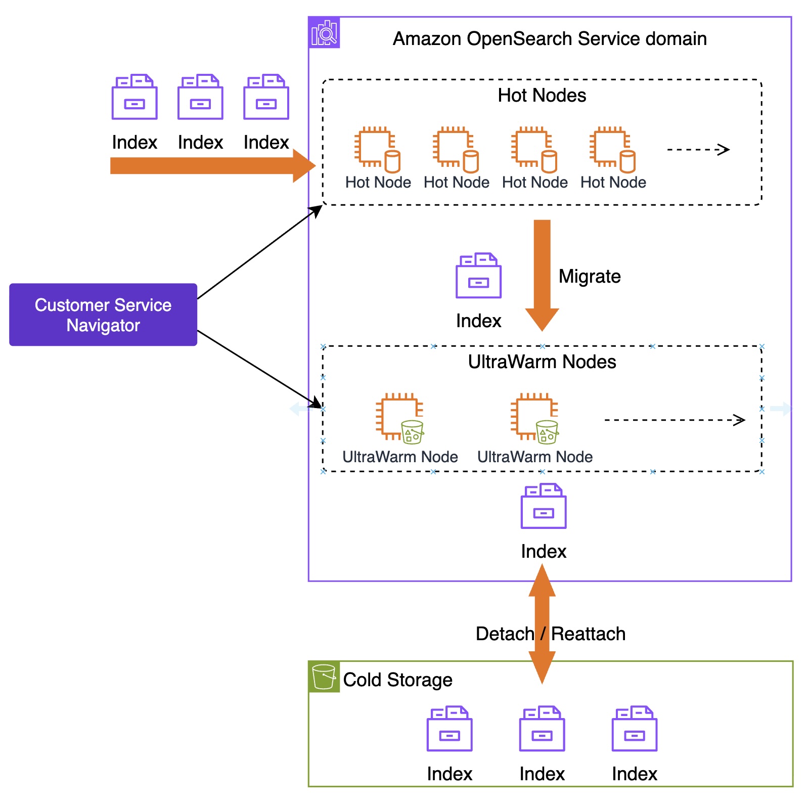
To manage the log, metric, and trace data at scale—about 3TB generated daily—the solution implemented OpenSearch Service storage tiering to balance performance, retention, and cost. Zeta requires near real-time search and retrieval for at least a week, while retaining logs and traces for up to 10 years. Keeping this data in active clusters would impact search performance and significantly increase costs, so the solution uses the OpenSearch Service hot, UltraWarm, and cold storage tiers to optimize the data lifecycle. The following diagram illustrates storage tiering in OpenSearch Service.

Zeta CSN Storage Tiering

Hot storage is used for the most recent and frequently accessed data, supporting real-time indexing and low-latency queries. This tier relies on high-performance storage attached to standard data nodes, making it ideal for powering live dashboards and analytics where speed is critical. The solution uses AWS Graviton 2 powered m6g.4xlarge.search instance types to run the OpenSearch Service domain which provides upto 40% lower cost compared to x86 based instances. Each hot data node has an attached gp3 EBS volume to store indexes. Zeta maintains data in hot storage for 1 week.

UltraWarm storage serves as a cost-effective layer for older, read-only data that is queried less frequently but still needs to remain searchable. UltraWarm nodes use Amazon Simple Storage Service (Amazon S3) as the backing store with an integrated caching mechanism, to retain large volumes of data at a fraction of the cost of hot storage while still supporting interactive queries for historical analysis. Zeta uses ultrawarm1.large.search instance types in the UltraWarm storage tier and maintains data in UltraWarm storage for 15 days.

Cold storage is designed for long-term archival of infrequently accessed or compliance-driven data. Data in cold storage is detached from active compute resources and resides in Amazon S3, incurring minimal cost. When historical data needs to be queried, the indexes are attached to the UltraWarm nodes using OpenSearch API calls. This helps extracting historical data for audits, periodic research or forensic investigations without maintaining active compute for the entire retention period, thereby reducing storage cost.

OpenSearch Service automates index transitions between hot, UltraWarm, and cold storage tiers using Index State Management (ISM) policies. ISM policies specify the conditions and actions for each state, such as transitioning based on index age, size, or document count. When an index qualifies for a transition, ISM jobs—running every 5 to 8 minutes—evaluate the policy and move the index to the next tier. When indexes reach the UltraWarm threshold, they are migrated to UltraWarm nodes backed by Amazon S3, which reduces storage costs while keeping data accessible for queries. After the UltraWarm retention period, ISM archives the indexes to cold storage, detaching them from compute resources but allowing reattachment for future queries or compliance needs. This automated lifecycle management reduces operational overhead, optimizes storage costs, and maintains performance for both recent and historical data.

For observability data, new indexes are created in the hot tier, where they remain for 7 days to support fast ingestion and low-latency queries. After this period, ISM transitions these indexes to UltraWarm storage, where they are retained for an additional 15 days as read-only data, balancing cost with searchability.

Security

Security is the most critical part of the architecture. Zeta’s observability system implements multiple layers of protection for data confidentiality, integrity, and compliance with banking regulations, and is built using a zero-trust approach following the AWS shared responsibility model for OpenSearch Service:

  • Infrastructure security: The OpenSearch Service domain is deployed within a virtual private cloud (VPC) with private subnets, isolating it from direct internet access. Security groups enforce restrictive ingress rules, allowing access only from authorized sources. The OpenSearch Service domain uses encryption at rest through AWS Key Management Service (KMS). Data in transit is secured using TLS 1.3 encryption, so that log data, traces, and search queries remain protected during transmission. Service-to-service communication uses AWS Identity and Access Management (IAM) roles and encrypted connections, alleviating the need for hardcoded credentials.
  • Access control and authentication: The solution uses Amazon OpenSearch Service fine-grained access control(FGAC) integrated with IAM, where IAM serves as the authentication provider and FGAC handles authorization by mapping IAM roles to OpenSearch backend roles. This approach helps Zeta to control access permissions at the index and document level based on tenant requirements and user responsibilities. The data ingestion pipeline implements end-to-end security with Fluentd authenticating to Amazon MSK using IAM roles over encrypted connections. Amazon MSK clusters use encryption in transit and at rest, protecting log data throughout the streaming pipeline. Kubernetes RBAC policies restrict pod-to-pod communication and limit service account permissions.
  • Data privacy and tenant isolation: Each tenants’ data is maintained in logical separation in OpenSearch Service using tenant id. CSN implements tenant-aware authentication and authorization with FGAC, restricting users to their authorized tenants’ dashboards and data. Every API endpoint validates tenant context, so that users can only access data within their authorized scope. Importantly, no customer data is captured in the logs – only system metrics are used to build the monitoring system, adhering to banking security standards and best practices. User actions are audited and logged for compliance purposes, with audit trails maintained according to regulatory requirements.

This security framework enables the observability system meet the security requirements of core banking operations while maintaining operational efficiency and regulatory compliance across global industries.

Customer Service Navigator

CSN delivers SREs a powerful diagnostics interface engineered for high-efficiency monitoring, deep analysis, and rapid troubleshooting of system performance across distributed environments. The system ingests and processes telemetry data at sub-minute intervals, providing near-real-time metrics, traces, and logs from critical infrastructure components. Actionable, interactive visualizations—such as heatmaps, anomaly graphs, and dependency maps— helps SREs to quickly detect SLO breaches and drill down to granular root causes, often within a few minutes of an incident.

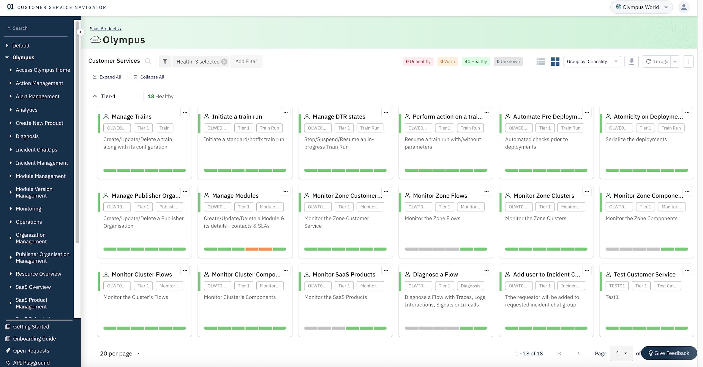
The following screenshot shows an example service health dashboard in CSN for an Olympus tenant.

Zeta CSN Service Health Dashboard

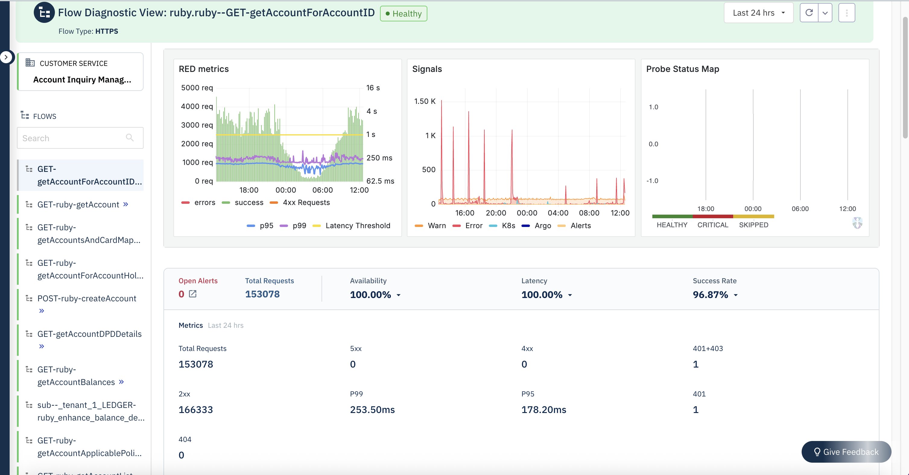
The following screenshot shows an example of the API performance insights dashboard in CSN.

Zeta CSN API Performance Dashboard

Business and technical benefits

The OpenSearch Service-based CSN System provides the following business and technical benefits:

  • Manual effort is reduced through automated Index State Management (ISM) and lifecycle policies, so that Zeta’s teams to focus on innovation
  • Automated lifecycle policies facilitate seamless retention and archiving of compliance data, reducing the risk of non-compliance
  • The system supports log retention for over 10 years to meet regulatory requirements for Zeta’s banking and financial services customers
  • Multiple layers of security—including encryption at rest and in transit, FGAC, and tenant isolation to protect customer data and support Zeta’s zero-trust architecture
  • By consolidating logs, traces, and metrics from disparate systems into OpenSearch, SRE teams can correlate events more effectively, thereby reducing troubleshooting efforts and achieving an 80% improvement in MTTR
  • Zeta achieved 99.999999999% data durability for archived logs stored in Amazon S3, providing long-term data integrity
  • Zstandard compression is being implemented to optimize long-term storage costs

Conclusion

CSN’s advanced correlation engine automatically associates related events across microservices, databases, network layers, and infrastructure, significantly streamlining root cause analysis. Integrated alerting and automated runbooks further reduce response times. Since implementing CSN, Zeta has achieved over an 80% reduction in MTTR, with incident response times decreasing from 30+ minutes to under 5 minutes. The service supports seamless multi-tenant monitoring, processes 3TB of machine-generated data daily, and is architected for petabyte-scale growth. Additionally, CSN helps Zeta meet regulatory requirements for retaining historical logs over several years while keeping storage costs under control. This has substantially improved operational resilience, increased service availability, and empowered teams to proactively resolve issues before they affect end users.

Ready to take your organization’s observability capabilities to the next level? Dive into the technical details of OpenSearch Service in the Amazon OpenSearch Developer Guide. Visit our new migration hub page for more prescriptive guidance on moving your workloads to OpenSearch Service.


About the authors

Deepesh DhapolaDeepesh Dhapola is a Senior Solutions Architect at AWS India, where he architects high-performance, resilient cloud solutions for financial services and fintech organizations. He specializes in using advanced AI technologies—including generative AI, intelligent agents, and the Model Context Protocol (MCP)—to design secure, scalable, and context-aware applications. With deep expertise in machine learning and a keen focus on emerging trends, Deepesh drives digital transformation by integrating cutting-edge AI capabilities to enhance operational efficiency and foster innovation for AWS customers. Beyond his technical pursuits, he enjoys quality time with his family and explores creative culinary techniques.

Shashidhar (Shashi) SoppinShashidhar (Shashi) Soppin is an accomplished Enterprise Architect and cloud transformation leader with over 24+ years of experience spanning regulated industries and high-growth technology environments. Currently steering strategic initiatives as Lead Architect at Zeta’s CTO office, Shashidhar has helped in building and led world-class engineering teams, driving innovation in cloud, security, and fintech domains. He has architected secure, scalable platforms—scaling user bases by 10x, enabling complex integrations for leading Bank’s migration to Zeta’s platforms, and pioneering Zero Trust frameworks that achieved outstanding regulatory compliance. A results-driven executive and former DMTS at Wipro, Shashidhar holds 25+ granted patents and has delivered multi-million dollar enterprise deals across domains including AI/ML. Renowned as a published author (“Essentials of Deep Learning”), frequent industry speaker, and hands-on innovator, he combines technical expertise with business acumen, propelling organizations toward robust, future-ready cloud ecosystems and operational excellence. Prior to Wipro he worked in IBM-ISL as well.

Anchal KansalAnchal Kansal is a Lead Site Reliability Engineer at Zeta, where she has spent the past four years building and scaling reliable, high-performance systems. With deep expertise in OpenSearch, observability platforms, and large-scale infrastructure, she focuses on ensuring uptime, performance, and operational efficiency. Anchal is passionate about solving complex reliability challenges and sharing practical insights with the engineering community.

Mano (Manochandra)Manochandra (Mano) is the Site Reliability Engineering (SRE) expert at Zeta, specializing in data management-oriented systems. With a deep understanding of large-scale distributed architectures, he has extensive experience designing, deploying, and maintaining resilient, production-grade OpenSearch systems. Mano is known for his proactive approach in optimizing infrastructure reliability and performance, as well as his ability to troubleshoot complex operational challenges. His expertise spans implementing automation, monitoring, and incident management best practices, making him a go-to resource for ensuring service availability and scalability at Zeta.

 Hitesh SubnaniHitesh Subnani is a FSI Solutions Architect at AWS India, where he works with customers to design and build architectures that deliver business value. He specializes in comprehensive observability and analytics systems, enabling organizations to gain deep insights from operational data. With expertise in search and analytics technologies, Hitesh focuses on scalable monitoring systems, real-time dashboards, and compliance-driven architectures for AWS customers in the financial sector.

Tarun ChakrabortyTarun Chakraborty is a Sr. Technical Account Manager (TAM) at AWS India, where he partners with leading banks and fintech organizations to accelerate their cloud transformation journeys. With over 15 years of experience in technology and financial services, he serves as a trusted advisor helping customers leverage AWS’s comprehensive suite of services to drive innovation and achieve their business objectives.

Multi-rack and multiple logical AWS Outposts architecture considerations for resiliency

Post Syndicated from Brianna Rosentrater original https://aws.amazon.com/blogs/compute/multi-rack-and-multiple-logical-aws-outposts-architecture-considerations-for-resiliency/

AWS Outposts rack offers the same Amazon Web Services (AWS) infrastructure, AWS services, APIs, and tools to virtually any on-premises data center or colocation space for a truly consistent hybrid experience. A logical Outpost (hereafter referred to as an Outpost) is a deployment of one or more physically connected Outposts racks managed as a single entity under one Amazon Resource Name (ARN). An Outpost provides a pool of AWS compute and storage capacity at one of your sites as a private extension of an Availability Zone (AZ) in an AWS Region. Several AWS services that support Outposts offer deployment options that improve your workload’s fault tolerance. However, certain Outposts configuration requirements have to be met in order to use them.

In this post, we explore the architecture considerations that come into play when deciding between a multi-rack logical Outposts rack, or using multiple Outposts racks to support your highly available workloads.

Amazon EC2 on AWS Outposts rack

The following sections cover Amazon Elastic Compute Cloud (Amazon EC2) on Outposts rack

Multi-rack logical Outposts

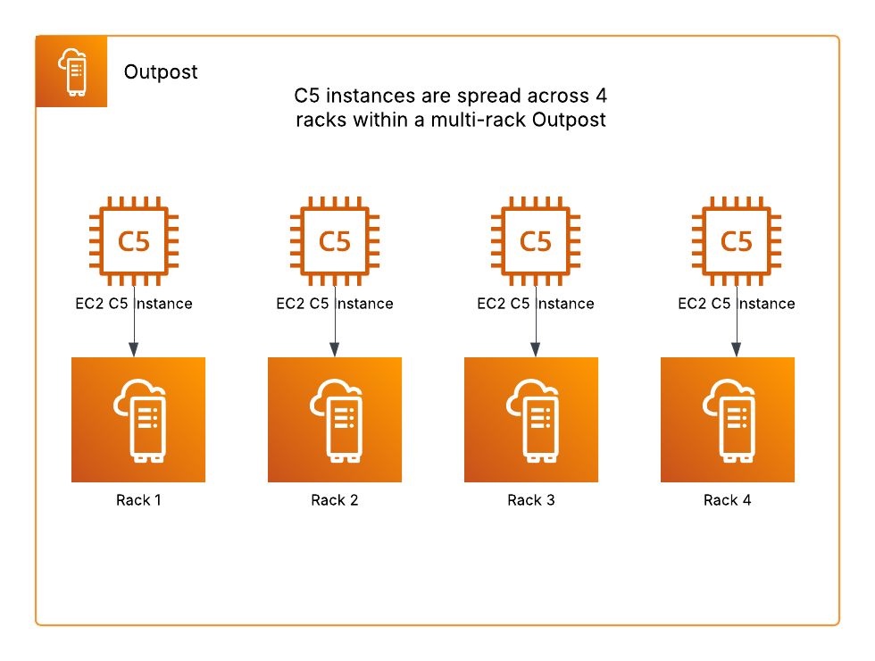
When using a multi-rack logical Outpost, you can use a rack level spread Amazon EC2 placement group. A rack level spread placement group can have as many partitions as you have racks in your Outpost deployment, and this allows you to spread out your instances to improve the fault tolerance of your workloads. In the following example, we have C5 instances in an Amazon EC2 Auto Scaling group that uses a launch template specifying a rack level spread placement group strategy should be used. This multi-rack Outpost has four racks, thus the instances are spread across the four racks as evenly as possible.

Rack level spread EC2 placement group example

Figure 1: Rack level spread Amazon EC2 placement group example

This placement group strategy can make your workloads more resilient to rack or host failures, but it would not be useful in mitigating an AZ failure. EC2 instances on Outposts are statically stable to network disconnects. Therefore, workloads would continue running during an AZ failure, but mutating actions would be unavailable. Read on to see how this strategy can be used with multiple Outposts to create a multi-AZ resilient architecture.

Multiple Outposts racks

If you have more than one logical Outpost in the same Region, we recommend connecting each Outpost to a different AZ. This would allow you to create multi-AZ resilient architectures, and when used in combination with features such as Intra-VPC communication between your Outposts, you can stretch an Amazon EC2 Auto Scaling group across two or more Outposts in the same VPC. If each Outpost is a single rack deployment, then this can be combined with a host level spread placement group specified in your instance launch template. A host level spread placement group can have as many partitions as you have hosts of that instance type in your Outpost, and would improve your workload’s resiliency to host failures.

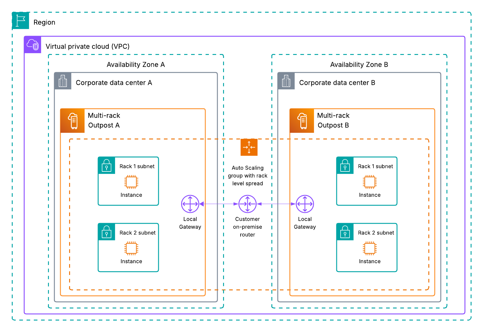
For the highest level of spread and resiliency, consider using multiple multi-rack logical Outposts. This would allow you to use rack level spread placement groups, and intra-VPC communication between Outposts, as shown in the following figure. Having more than one multi-rack Outpost allows you to create application architectures that are resilient toward hardware and AZ level failures by spreading your workload across as many fault domains as possible.

Intra-VPC communication between two multi-rack logical Outposts using an EC2 auto scaling group with rack level spread

Figure 2: Intra-VPC communication between two multi-rack logical Outposts using an Amazon EC2 Auto Scaling group with rack level spread

Amazon RDS on AWS Outposts rack

The following sections cover Amazon Relational Database Service (Amazon RDS) on Outposts rack.

Multi-rack logical Outposts

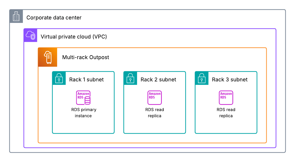
Amazon RDS on Outposts rack supports read replicas, which use the MySQL and PostgreSQL database engines’ built-in asynchronous replication functionality to create a read replica from a source database instance. Read replicas on Amazon RDS on Outposts can be located on the same Outpost or another Outpost in the same VPC as the source database instance, as shown in the following figure. Furthermore, these can be used to scale out beyond the capacity constraints of a single database instance for read-heavy database workloads. They can also be used to maintain a second copy of your database, which can be used in the event of a host failure to improve workload resiliency. The process to promote a read replica to primary must be manually initiated, and your DNS records must be updated to the new primary instance. However, this is a good option to improve database durability if you only have one logical Outpost. Multiple read replicas can be created for a single database instance for added resiliency. You can also create an Amazon RDS read replica for a single rack Outpost to improve your resiliency to host failures. However, having a multi-rack Outpost would allow you to spread your read replica to another rack within your Outpost.

RDS read replicas used with a multi-rack Outpost

Figure 3: Amazon RDS read replicas used with a multi-rack Outpost

Multiple Outposts racks

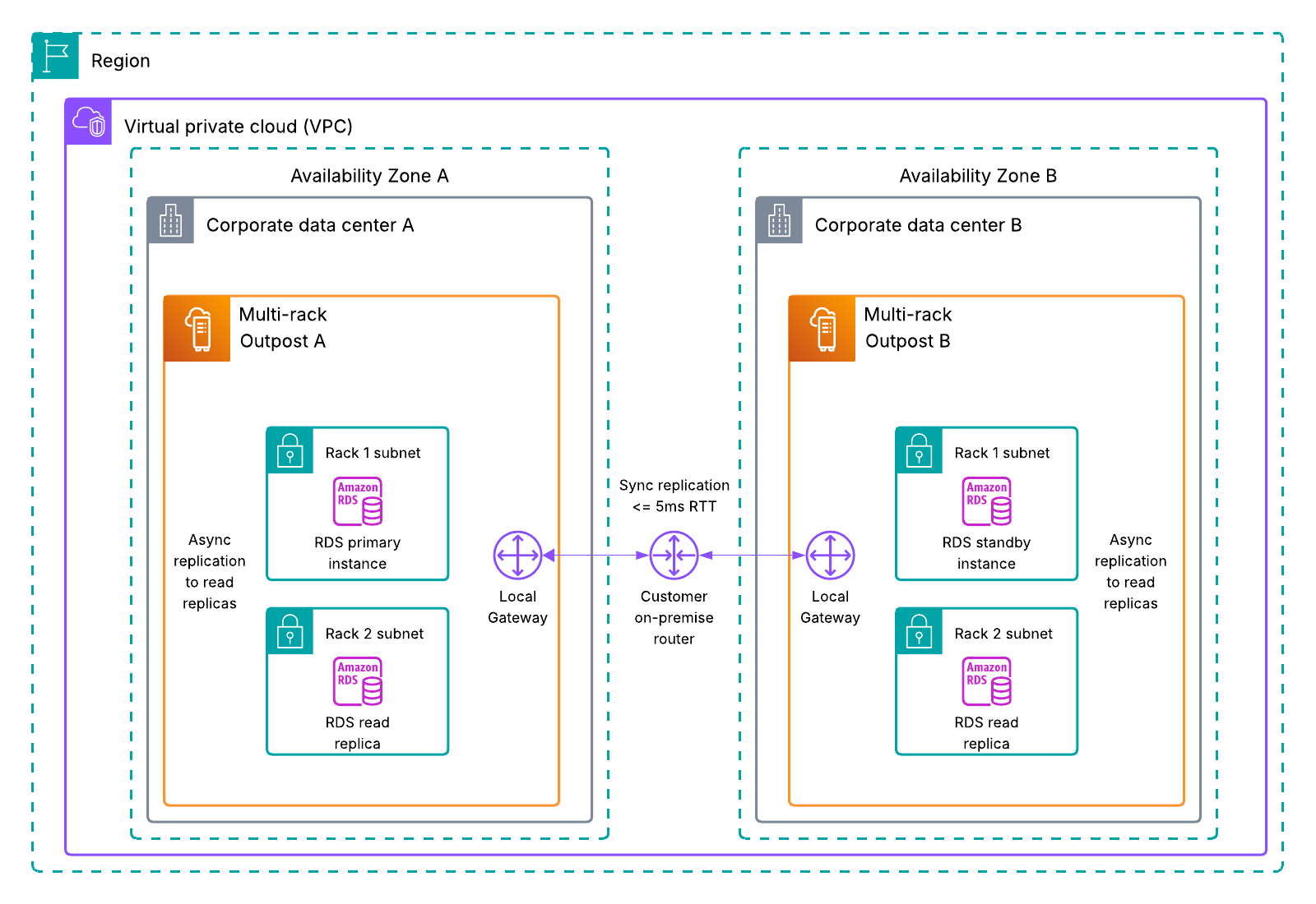
Multi-AZ Amazon RDS deployments are supported on Outposts rack for MySQL and PostgreSQL database instances, as shown in the following figure. Using your Outposts Local Gateway and synchronous data replication, Amazon RDS creates a primary database instance on one Outpost, and maintains a standby database instance on a different Outpost. Failover to a multi-AZ Amazon RDS standby instance is automatic, and the DNS records are also automatically updated as part of the failover process. Using this deployment option protects you from AZ, host, and Outpost failures. You can also use multi-AZ Amazon RDS in combination with read replicas spread across different hosts on the same rack, or across multiple racks if using two multi-rack Outposts to provide more database durability.

Multi-AZ RDS on Outposts using read replicas for added durability.

Figure 4: Multi-AZ Amazon RDS on Outposts using read replicas for added durability

Amazon EKS on Outposts rack

The following sections cover Amazon Elastic Kubernetes Service (Amazon EKS) on Outposts rack.

Multi-rack logical Outposts

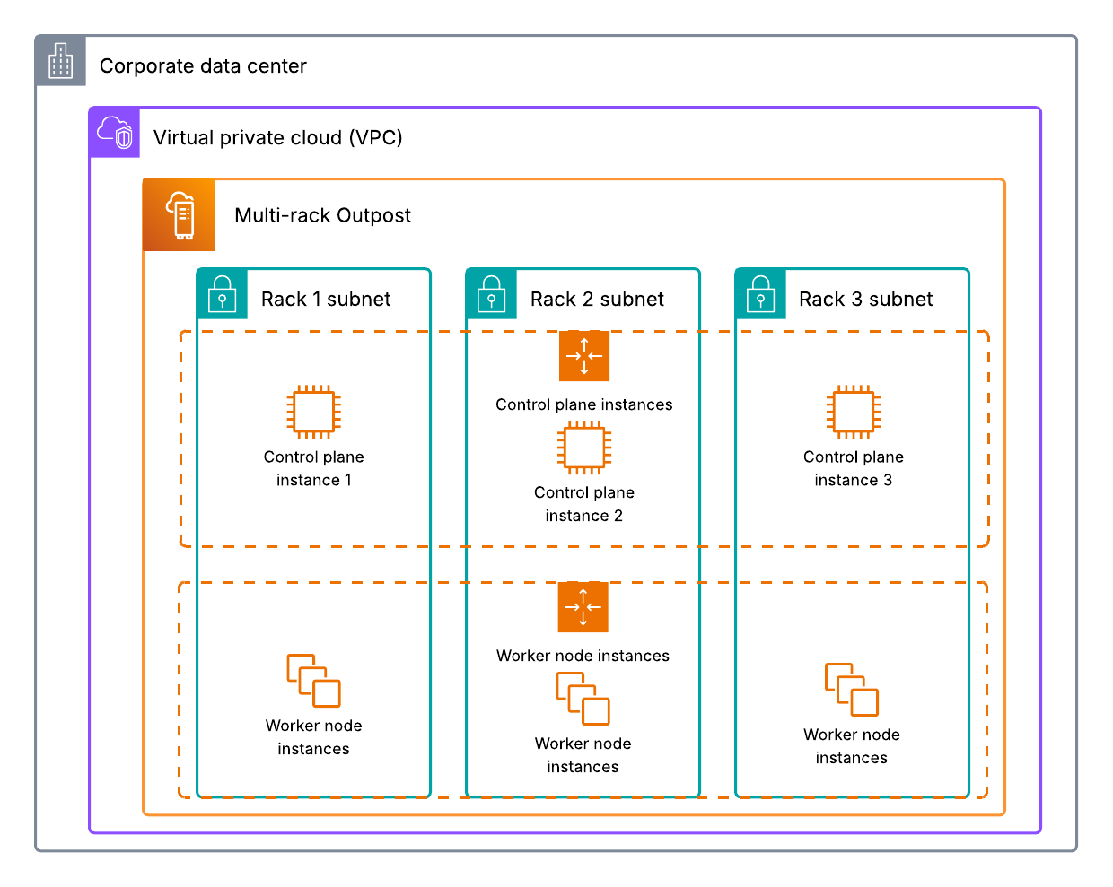
Outposts rack supports two Amazon EKS deployment methods: EKS extended cluster, and EKS local cluster, as shown in the following figure. Go to our documentation for help deciding which method is right for your workload. Using the rack level placement group strategy discussed earlier in this post allows you to spread your EKS instances (worker and control plane depending on the deployment model used) across multiple racks within your Outpost. Amazon EKS control plane instances are automatically replaced in the event of an instance, host, or rack failure, and self-managed worker node instances are typically placed in an Amazon EC2 Auto Scaling group. Therefore, when they’re used with a rack level spread placement group, you can increase your Amazon EKS resiliency and use automation to handle failures.

EKS local cluster with rack level spread placement group and auto scaling

Figure 5: EKS local cluster with rack level spread placement group and auto scaling

Multiple Outposts racks

When using multiple Outposts racks, you’re unable to spread EKS control plane instances across two disparate Outposts. Go to Deploy an Amazon EKS cluster across AWS Outposts with Intra-VPC communication for more information on how to stretch an EKS extended cluster across multiple Outposts racks. If EKS local cluster is a requirement for your workload, you could use an external load balancer and deploy one instance of EKS local cluster on each Outpost in an active/active or active/passive configuration, and use the load balancer to direct incoming traffic to each respective EKS cluster. If your EKS cluster is using persistent storage, then you should consider whether each cluster needs access to the other clusters data, and centralized storage or replication should be used if needed.

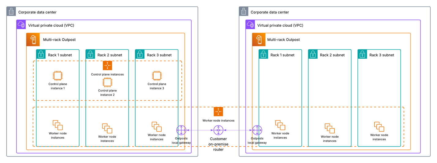
Alternatively, if you are using EKS local cluster with two single rack Outposts, then you can also choose to only spread your EKS worker node instances across both of your Outposts. Furthermore, you can use host level spread on your primary Outpost to provide host level resiliency for your control plane instances. This would provide some added durability in the event of a host failure, and you could withstand the failure of your secondary Outpost that is only running some of your worker node instances. If you have two multi-rack Outposts, even though you couldn’t spread your control plane instances across Outposts, you can still use a rack level spread placement group to spread them across racks within your primary multi-rack Outpost. This would provide resiliency against instance, host, rack, and AZ level failures, and you could withstand the failure of your secondary multi-rack Outpost that isn’t running your EKS control plane instances as well.

EKS local cluster using two multi-rack Outposts and rack level spread

Figure 6: EKS local cluster using two multi-rack Outposts and rack level spread

Amazon S3 on Outposts rack

The following sections cover Amazon S3 on Outposts rack.

Multi-rack logical Outposts

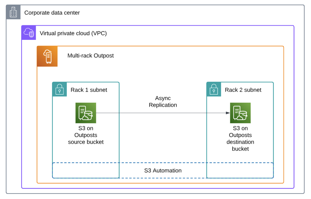
Amazon S3 on Outposts supports object replication, either across distinct Outposts, or between buckets on the same Outpost to help meet data-residency needs. The Outpost or bucket you’re replicating to can be in the same AWS account, or a different account. If you have a multi-rack Outpost, then you can replicate your S3 objects to another bucket on the same Outpost to create a copy of your data locally for added resiliency.

S3 replication between buckets on the same Outpost

Figure 7: Amazon S3 replication between buckets on the same Outpost

Multiple Outposts racks

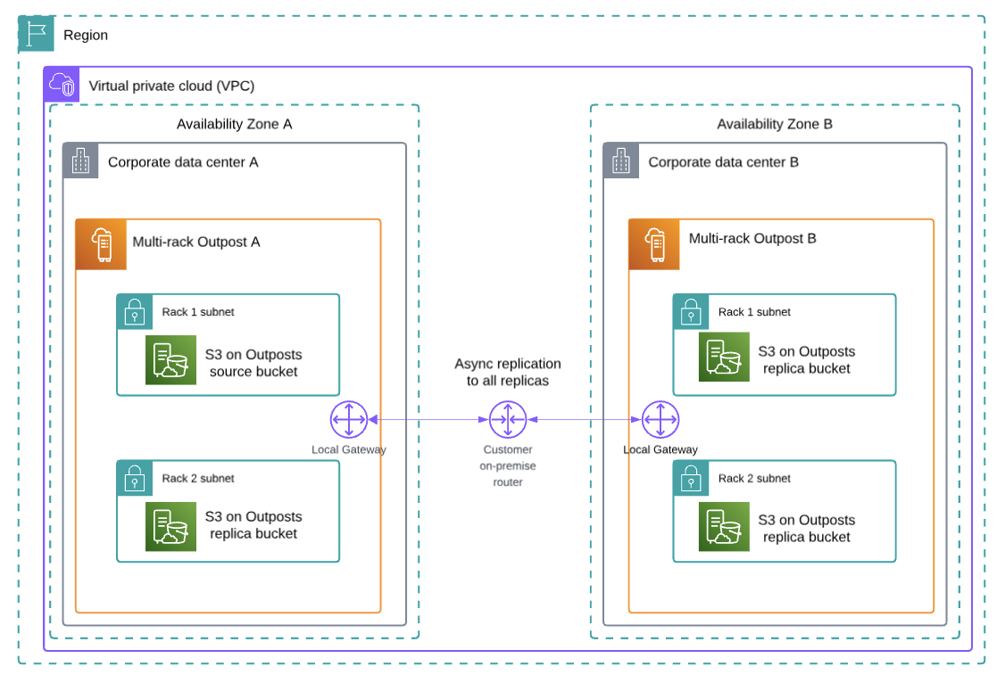
Moreover, if you have multiple Outposts, then you can replicate S3 objects between buckets on each Outpost, as shown in the following figure. Connect each Outpost to a unique AZ to create a multi-AZ resilient architecture, and store a copy of your data on each Outpost. You can combine this with Amazon S3 replication to a bucket on the same Outpost as well, and have multiple replicas managed through Amazon S3 automation for the highest availability. AWS DataSync also supports Amazon S3 on Outposts, and can be used to replicate S3 objects to the Region your Outpost is connected to if you want to store a copy of your data in the cloud, or use Amazon S3 in the Region for data tiering. Refer to Automate data synchronization between AWS Outposts racks and Amazon S3 with AWS DataSync for more information.

S3 replication across two multi-rack Outposts

Figure 8: Amazon S3 replication across two multi-rack Outposts

Further considerations

  • When using multiple Outposts, we recommend connecting each Outpost to a unique availability zone to use multi-AZ deployment options.
  • Outposts are designed to be a connected service, and network outages could cause workflow disruptions. AWS can help you design for continued operations during network outages. We recommend creating a redundant service link connection to support workloads on Outposts with high availability requirements. Go to AWS Direct Connect Resiliency Recommendations for guidance on how to create a highly available service link connection through AWS Direct Connect, and Satellite Resiliency for AWS Outposts.
  • Outposts have a finite amount of compute resources based on the physical configuration chosen, and the logical capacity configuration on your Outpost can be changed at any time using a capacity task. If the Amazon EC2 compute requirements for your workload change over time, then your Outposts capacity configuration can be updated to meet these requirements non-disruptively. Go to Dynamically reconfigure your AWS Outposts capacity using Capacity Tasks for more information.

Conclusion

This post explores the architecture options and considerations for deciding between a multi-rack Outpost, and using multiple Outposts to support your highly available workloads. For more information on how to design highly available architecture patterns for Outposts, go to the AWS Outposts High Availability Design and Architecture Considerations whitepaper. Reach out to your AWS account team, or fill out this form to learn more about Outposts and self-service capacity management.

Build enterprise-scale log ingestion pipelines with Amazon OpenSearch Service

Post Syndicated from Akhil B original https://aws.amazon.com/blogs/big-data/build-enterprise-scale-log-ingestion-pipelines-with-amazon-opensearch-service/

Organizations of all sizes generate massive volumes of logs across their applications, infrastructure, and security systems to gain operational insights, troubleshoot issues, and maintain regulatory compliance. However, implementing log analytic solutions presents significant challenges, including complex data ingestion pipelines and the need to balance cost and performance while scaling to handle petabytes of data.

Amazon OpenSearch Service addresses these challenges by providing high-performance search and analytics capabilities, making it straightforward to deploy and manage OpenSearch clusters in the AWS Cloud without the infrastructure management overhead. A well-designed log analytics solution can help support proactive management in a variety of use cases, including debugging production issues, monitoring application performance, or meeting compliance requirements.

In this post, we share field-tested patterns for log ingestion that have helped organizations successfully implement logging at scale, while maintaining optimal performance and managing costs effectively.

Solution overview

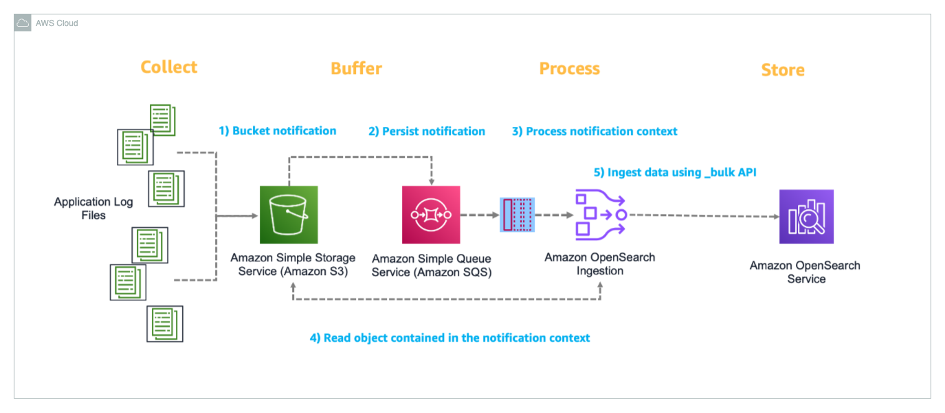
Organizations can choose from several data ingestion architectures, such as:

Irrespective of the chosen pattern, a scalable log ingestion architecture should comprise the following logical layers:

  • Collect layer – This is the initial stage where logs are gathered from various sources, including application logs, system logs, and more.
  • Buffer layer – This layer acts as a temporary storage layer to handle spikes in log volume and prevents data loss during downstream processing issues. This layer also maintains system stability during high load.
  • Process layer – This layer transforms the unstructured logs into structured formats while adding relevant metadata and contextual information needed for effective analysis.
  • Store layer – This layer is the final destination for processed logs (OpenSearch in this case), which supports various access patterns, including querying, historical analysis, and data visualization.

OpenSearch Ingestion offers a purpose-built, fully managed experience that simplifies the data ingestion process. In this post, we focus on using OpenSearch Ingestion to load logs from Amazon Simple Storage Service (Amazon S3) into an OpenSearch Service domain, a common and efficient pattern for log analytics.

OpenSearch Ingestion is a fully managed, serverless data ingestion service that streamlines the process of loading data into OpenSearch Service domains or Amazon OpenSearch Serverless collections. It’s powered by Data Prepper, an open source data collector that filters, enriches, transforms, normalizes, and aggregates data for downstream analysis and visualization.

OpenSearch Ingestion uses pipelines as a mechanism that consists of the following major components:

  • Source – The input component of a pipeline. It defines the mechanism through which a pipeline consumes records.
  • Buffer – A persistent, disk-based buffer that stores data across multiple Availability Zones to enhance durability. OpenSearch Ingestion dynamically allocates OCUs for buffering, which increases pricing as you may need additional OCUs to maintain ingestion throughput.
  • Processors – The intermediate processing units that can filter, transform, and enrich records into a desired format before publishing them to the sink. The processor is an optional component of a pipeline.
  • Sink – The output component of a pipeline. It defines one or more destinations to which a pipeline publishes records. A sink can also be another pipeline, so you can chain multiple pipelines together.

Because of its serverless nature, OpenSearch Ingestion automatically scales to accommodate varying workload demands, alleviating the need for manual infrastructure management while providing built-in monitoring capabilities. Users can focus on their data processing logic rather than spending time on operational complexities, making it an efficient solution for managing data pipelines in OpenSearch environments.

The following diagram illustrates the architecture of the log ingestion pipeline.

Let’s walk through how this solution processes Apache logs from ingestion to visualization:

  1. The source application generates Apache logs that need to be analyzed and stores them in an S3 bucket, which acts as the central storage location for incoming log data. When a new log file is uploaded to the S3 bucket (ObjectCreate event), Amazon S3 automatically triggers an event notification that is configured to send messages to a designated Amazon Simple Queue Service (Amazon SQS) queue.
  2. The SQS queue reliably manages and tracks the notifications of new files uploaded to Amazon S3, making sure the file event is delivered to the OpenSearch Ingestion pipeline. A dead-letter queue (DLQ) is configured to capture failed event processing.
  3. The OpenSearch Ingestion pipeline monitors the SQS queue, retrieving messages that contain information about newly uploaded log files. When a message is received, the pipeline reads the corresponding log file from Amazon S3 for processing.
  4. After the log file is retrieved, the OpenSearch Ingestion pipeline parses the content, and uses the OpenSearch Bulk API to efficiently ingest the processed log data into the OpenSearch Service domain, where it becomes available for search and analysis.
  5. The ingested data can be visualized and analyzed through OpenSearch Dashboards, which provides a user-friendly interface for creating custom visualizations, dashboards, and performing real-time analysis of the log data with features like search, filtering, and aggregations.

In the following sections, we guide you through the steps to ingest application log files from Amazon S3 into OpenSearch Service using OpenSearch Ingestion. Additionally, we demonstrate how to visualize the ingested data using OpenSearch Dashboards.

Prerequisites

This post assumes you have the following:

Deploy the solution

The solution uses a Python AWS Cloud Development Kit (AWS CDK) project to deploy an OpenSearch Service domain and associated components. This project demonstrates event-based data ingestion into the OpenSearch Service domain in a no code approach using OpenSearch Ingestion pipelines.

The deployment is automated using the AWS CDK and comprises the following steps:

  1. Clone the GitHub repo.
    git clone [email protected]:aws-samples/sample-log-ingestion-pipeline-for-amazon-opensearch-service.git

  2. Create a virtual environment and install the Python dependencies:
python3 -m venv .venv
source .venv/bin/activate
pip install -r requirements.txt
  1. Update the following environment variables in cdk.json:
    1. domain_name: The OpenSearch domain to be created in your AWS account.
    2. user_name: The user name for the internal primary user to be created within the OpenSearch domain.
    3. user_password: The password for the internal primary user.

This deployment creates a public-facing OpenSearch domain but is secured through fine-grained access control (FGAC). For production workloads, consider deploying within a virtual private cloud (VPC) with additional security measures. For more information, see Security in Amazon OpenSearch Service.

  1. Bootstrap the AWS CDK stack and initiate the deployment. Provide your AWS account number and the AWS Region where you want deploy the solution:
cdk bootstrap <Account ID>/<region>
cdk deploy --all

The process takes about 30–45 minutes to complete.

Verify the solution resources

When the previous steps are complete, you can check for the created resources.

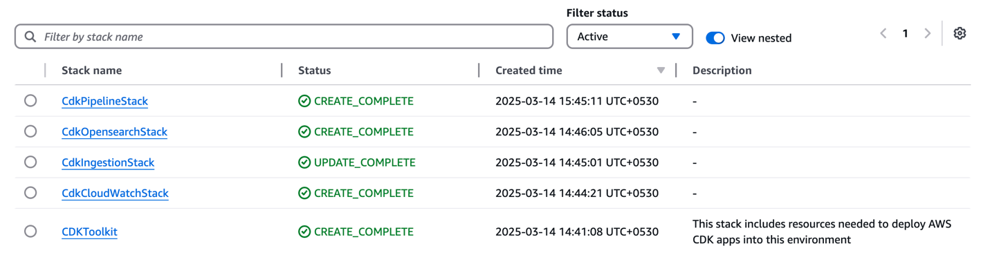
You can confirm the existence of the stacks on the AWS CloudFormation console. As shown in the following screenshot, the CloudFormation stacks have been created and deployed by cdk bootstrap and cdk deploy.

image-2

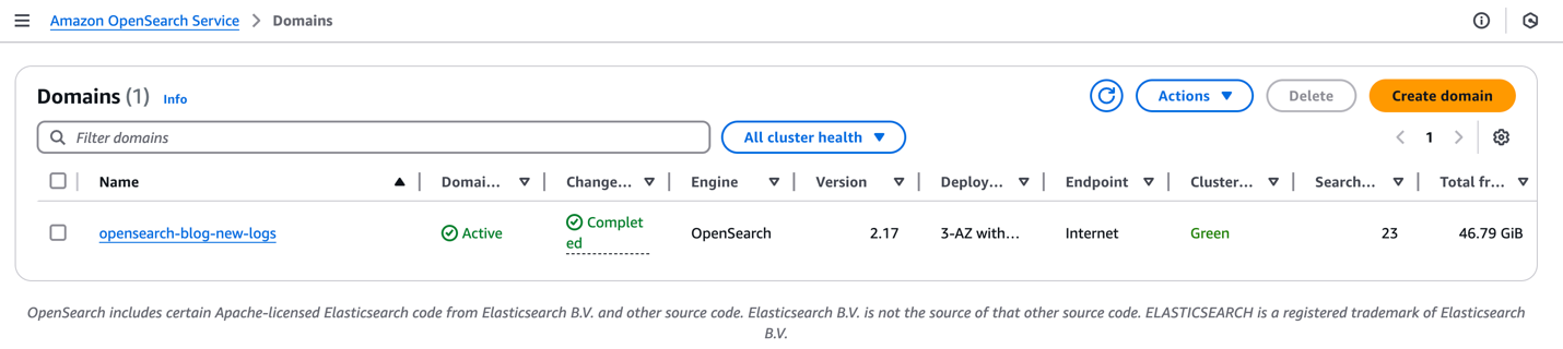
On the OpenSearch Service console, under Managed clusters in the navigation pane, choose Domains. You can confirm the domain created.

image-3

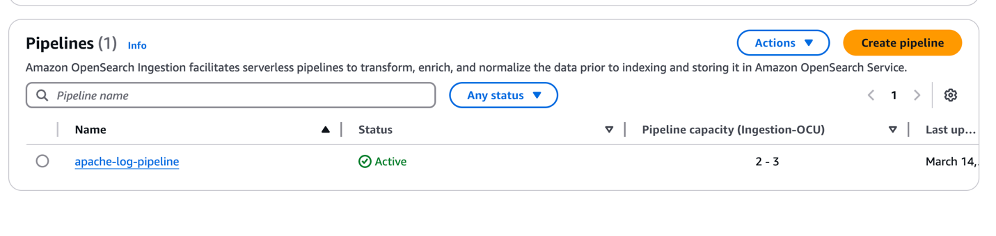
On the OpenSearch Service console, under Ingestion in the navigation pane, choose Pipelines. You can see the pipeline apache-log-pipeline created.

image-4

Configure security options

To configure your security roles, complete the following steps:

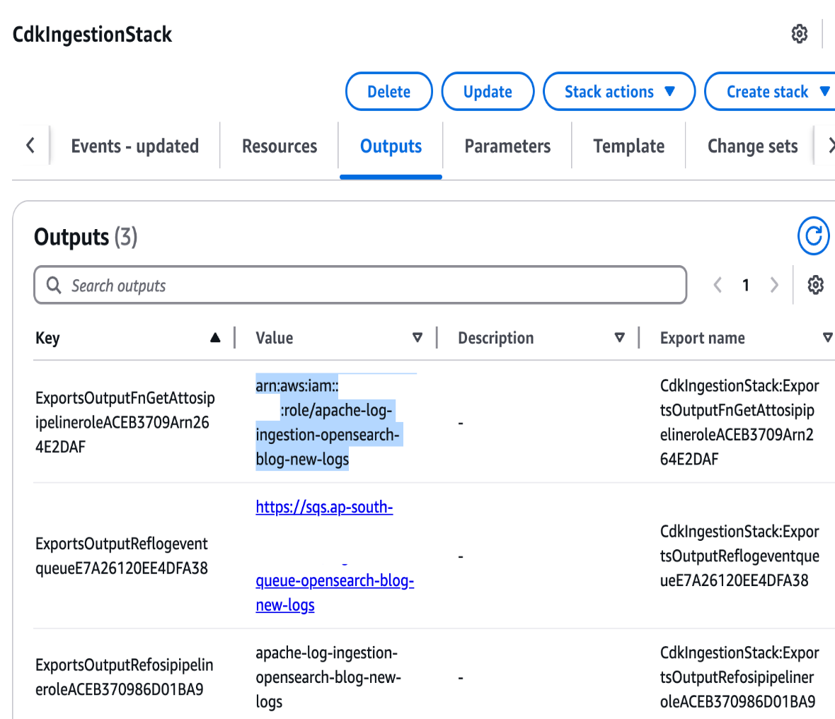
  1. On the AWS CloudFormation console, open the stack CdkIngestionStack, and on the Outputs tab, copy the Amazon Resource Name (ARN) of osi-pipeline-role.

image-5

  1. Open the OpenSearch Service console in the deployed Region within your AWS account and choose the domain you created.
  2. Choose the link for OpenSearch Dashboards URL.
  3. In the login prompt, enter the user credentials that were provided in cdk.json.

After a successful login, the OpenSearch Dashboards console will be displayed.

  1. If you’re prompted to select a tenant, select the Global tenant.
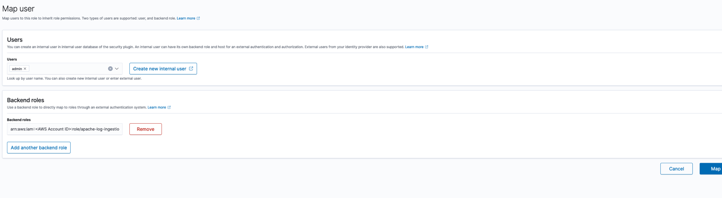
  2. In the Security options, navigate to the Roles section and choose the all_access role.
  3. On the all_access role page, navigate to mapped_users and choose Manage.
  4. Choose Add another backend role under Backend roles and enter the IAM role ARN you copied.
  5. Confirm by choosing Map.

image-6

Create an index template

The next step is to create an index template. Complete the following steps:

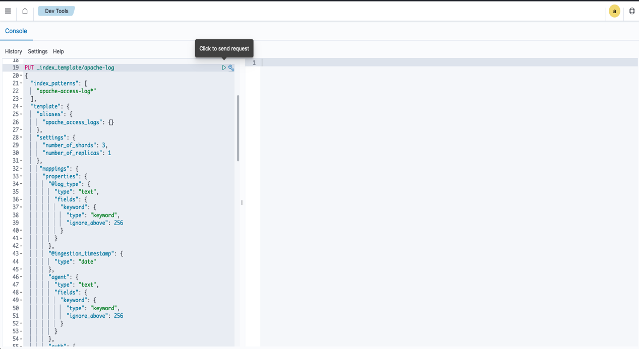
  1. On the Dev Tools console, copy the contents of the file index_template.txt within the opensearch_object directory.
  2. Enter the code in the Dev Tools console.

This index template defines the mapping and settings for our OpenSearch index.

  1. Choose the play icon to submit the request and create a template.

image-7

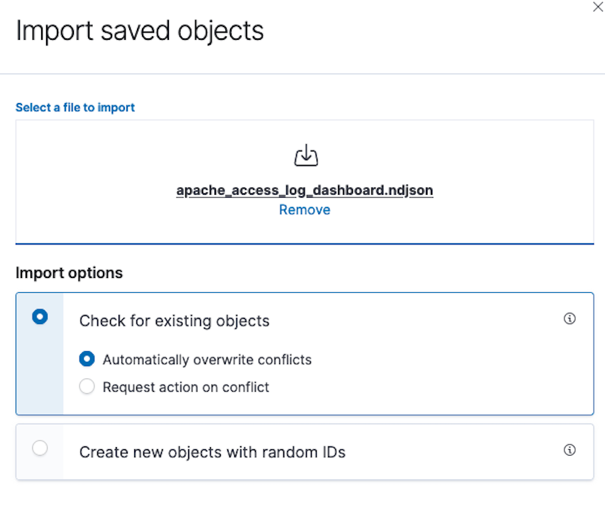
  1. In the Dashboard Management section, choose Saved Objects and choose Import.
  2. Choose Import and choose the apache_access_log_dashboard.ndjson file within the opensearch_object directory.
  3. Choose Check for existing objects.
  4. Choose Automatically overwrite conflicts and choose Import.

Ingest data

Now you can proceed with the data ingestion.

  1. On the Amazon S3 console, open the S3 bucket opensearch-logging-blog-<Account ID>.
  2. Upload the data file apache_access_log.gz (within the apache_log_data directory). The file can be uploaded in any prefix.

For this solution, we use Apache access logs as our example data source. Although this pipeline is configured for Apache log format, it can be modified to support other log types by adjusting the pipeline configuration. See Overview of Amazon OpenSearch Ingestion for details about configuring different log formats.

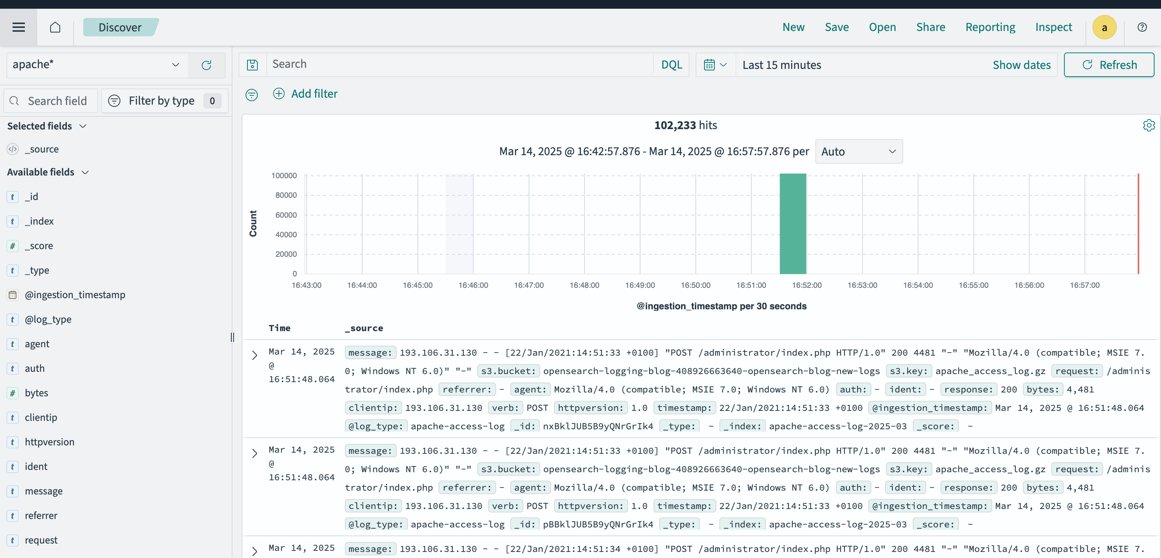
  1. After a few minutes, navigate to the Discover tab in OpenSearch Dashboards, where you can find that the data is ingested.
  2. Confirm that the apache* index pattern is selected.

image-8

  1. 5. On the Dashboards tab, choose Apache Log Dashboard.

The dashboard will be populated by the data and visuals should be displayed.

image-10

Operational best practices

When designing your log analytics platform on OpenSearch Service, make sure you follow the recommended operational best practices for cluster configuration, data management, performance, monitoring, and cost optimization. For detailed guidance, refer to Operational best practices for Amazon OpenSearch Service.

Clean up

To avoid ongoing charges for the resources that you created, delete them by completing the following steps:

  1. On the Amazon S3 console, open the bucket opensearch-logging-blog-<Account ID> and choose Empty.
  2. Follow the prompts to delete the contents of the bucket.
  3. Delete the AWS CDK stacks using the following command:
cdk destroy --all --force

Conclusion

As organizations continue to generate increasing volumes of log data, having a well-architected logging solution becomes crucial for maintaining operational visibility and meeting compliance requirements.

Implementing a robust logging infrastructure requires careful planning. In this post, we explored a field-tested approach in building a scalable, efficient, and cost-effective logging solution using OpenSearch Ingestion.

This solution serves as a starting point that can be customized based on specific organizational needs while maintaining the core principles of scalability, reliability, and cost-effectiveness.

Remember that logging infrastructure is not a “set-and-forget” system. Regular monitoring, periodic reviews of storage patterns, and adjustments to index management policies will help make sure your logging solution continues to serve your organization’s evolving needs effectively.

To dive deeper into OpenSearch Ingestion implementation, explore our comprehensive Amazon OpenSearch Service Workshops, which include hands-on labs and reference architectures. For additional insights, see Build a serverless log analytics pipeline using Amazon OpenSearch Ingestion with managed Amazon OpenSearch Service. You can also visit our Migration Hub if you’re ready to migrate legacy or self-managed workloads to OpenSearch Service.


About the authors

Akhil B is a Data Analytics Consultant at AWS Professional Services, specializing in cloud-based data solutions. He partners with customers to design and implement scalable data analytics platforms, helping organizations transform their traditional data infrastructure into modern, cloud-based solutions on AWS. His expertise helps organizations optimize their data ecosystems and maximize business value through modern analytics capabilities.

Ramya Bhat is a Data Analytics Consultant at AWS, specializing in the design and implementation of cloud-based data platforms. She builds enterprise-grade solutions across search, data warehousing, and ETL that enable organizations to modernize data ecosystems and derive insights through scalable analytics. She has delivered customer engagements across healthcare, insurance, fintech, and media sectors.

Chanpreet Singh is a Senior Consultant at AWS, specializing in the Data and AI/ML space. He has over 18 years of industry experience and is passionate about helping customers design, prototype, and scale Big Data and Generative AI applications using AWS native and open-source tech stacks. In his spare time, Chanpreet loves to explore nature, read, and spend time with his family.

Zig version 0.15.1

Post Syndicated from daroc original https://lwn.net/Articles/1034583/

The Zig project has
announced version 0.15.1 of the language. The release, much like the
last one, includes incremental progress toward the goal of completely dropping LLVM and improving compile time, as well as a handful of breaking changes as the language team wrestles with past API design. The biggest change this time around is to the standard library Reader and Writer interfaces, which have been completely rearranged in the name of performance and reducing unneeded copies.

All existing std.io readers and writers are deprecated in favor of the newly provided std.Io.Reader and std.Io.Writer which are non-generic and have the buffer above the vtable – in other words the buffer is in the interface, not the implementation. This means that although Reader and Writer are no longer generic, they are still transparent to optimization; all of the interface functions have a concrete hot path operating on the buffer, and only make vtable calls when the buffer is full.

These changes are extremely breaking. I am sorry for that, but I have carefully examined the situation and acquired confidence that this is the direction that Zig needs to go. I hope you will strap in your seatbelt and come along for the ride; it will be worth it.

Ново престъпление срещу природата до Алепу Kорупционна схема превръща защитени гори в бетон до Ропотамо

Post Syndicated from Екип на Биволъ original https://bivol.bg/alepu_beton.html

сряда 20 август 2025


     Символът на строителното безумие и държавната политика на системно унищожаване на природните ни богатства стана преди години т.нар. хотел „Подпорна стена“, който „Главбулгарстрой“ започна да строи направо на…

Материалът <span style='color:#ff0000;font-size:12px;'>Ново престъпление срещу природата до Алепу</span> <BR> <H1 class='post-title single-post-title entry-title'>Kорупционна схема превръща защитени гори в бетон до Ропотамо</H1> е публикуван за пръв път на Bivol!.

A Complete Guide to Resource Sharing for AWS End User Messaging

Post Syndicated from Brett Ezell original https://aws.amazon.com/blogs/messaging-and-targeting/a-complete-guide-to-resource-sharing-for-aws-end-user-messaging/

Introduction

Do you need to send SMS across multiple AWS accounts? Or have you ever wanted to use the same specific 10DLC phone number or branded Sender ID across those accounts? Perhaps your development team needs to test an application in a sandbox account using a production-ready number, or you’re migrating a workload to a new account and need to ensure your customer communications aren’t disrupted. Centralizing your messaging resources across accounts improves efficiency and branding, while lowering the risk in compliance gaps..

In this step-by-step guide, we will show how to solve this challenge by sharing your AWS End User Messaging resources across multiple AWS accounts using AWS Resource Access Manager (AWS RAM). By creating a single sharing account for your messaging resources—like phone numbers, Sender IDs, and opt-out lists—and securely sharing them with your other “consuming” accounts, you can build a more efficient, secure, and scalable communication platform.

Common Use Cases for Resource Sharing

Important: resource sharing with AWS RAM is a regional feature. You can only share resources with accounts within the same AWS Region where those resources are located.

Centralizing and sharing resources is a powerful pattern that addresses several common customer needs:

  • Testing in a Sandbox Environment: Allows development teams to test applications using production-ready phone numbers or Sender IDs in an isolated sandbox account, without giving them access to production configurations.
  • Simplified Registration and Onboarding: Share an existing pre-registered 10DLC number or Sender ID with a new account that has not yet completed its own registration process, enabling it to start sending messages more quickly.
  • Seamless Account Transitions: When migrating an application or workload to a new AWS account, you can share the existing origination identities. This makes certain that your phone numbers and Sender IDs remain consistent during the transition, preventing any disruption to your customer-facing communications.

This guide will walk you through the step-by-step process of sharing your AWS End User Messaging resources.

Shareable AWS End User Messaging Resources

You can share the following AWS End User Messaging resources using AWS RAM:

  • Phone Numbers: Share your dedicated short codes, 10DLCs, long codes, and toll-free numbers. This allows different accounts to send messages using a centralized pool of numbers.
  • Sender IDs: Share alphanumeric sender IDs to maintain consistent branding in one-way SMS messages across your accounts.
  • Opt-out Lists: Centralize your opt-out management to ensure regulatory compliance. When a user opts out of messaging from one account, they are opted out across all accounts using that shared list. This is especially powerful when used with pools, as you can associate a pool with a specific opt-out list, ensuring all numbers in that pool adhere to the same primary list. As a best practice, you should create and share a dedicated opt-out list rather than relying on the default list for each account.
  • Pools: Share your pools of phone numbers and sender IDs to manage origination identities at scale. Pools provide benefits like automatic failover and apply settings like opt-out lists or two-way SMS configurations to the entire pool.
    • Important: for a shared Opt-out list or pool to be functional, all of its member resources (the phone numbers and/or Sender IDs within it) must also be included in the same AWS RAM resource share.

Understanding AWS RAM Fundamentals

Before sharing your End User Messaging resources, it’s essential to understand the core concepts of AWS RAM.

  • Resource Share: This is the central component in AWS RAM. A resource share consists of three elements:
    • The resources to be shared (such as phone numbers, or opt-out lists).
    • The principals (AWS accounts, OUs, or an entire organization) with whom you are sharing.
    • The managed permissions that define what actions the principals can perform on the shared resources.

Important: The supported resources of AWS End User Messaging are shareable with AWS accounts, Organizations, and OUs, but not with individual AWS Identity and Access Management (IAM) roles or users. This restriction ensures that resource sharing remains at the account level, maintaining clear boundaries and simplifying access management for your End User Messaging infrastructure.

  • Sharing Account vs. Consuming Account:
    • The sharing account (or owner account) is the AWS account that owns the resources and creates the resource share.
    • When a principal (such as an AWS account) is granted access to a resource share, it becomes a consuming account. It can use the shared resources according to the permissions granted and pays for its own usage of those resources, not for the resources themselves. For example: The consuming account pays for the volume of SMS sent by a shared number but the sharing account pays for any fees associated with owning that actual number.
  • AWS Organizations Integration: While you can share resources with individual AWS accounts, the most powerful way to use AWS RAM is in conjunction with AWS Organizations. This service allows you to centrally manage and govern multiple AWS accounts under a single umbrella. When you enable sharing within your organization, you can share resources with all accounts in the organization, or with specific Organizational Units (OUs), seamlessly and without needing to send and accept individual invitations. This sharing is only possible between accounts that reside in the same AWS Region.
  • Managed Permissions: AWS RAM uses managed permissions to control access.
    • AWS managed permissions are predefined permission sets created and maintained by AWS for common use cases. For AWS End User Messaging, the key permission is AWSRAMDefaultPermissionSmsVoice, which allows consumers to use the resources for sending messages but not for deleting or modifying them.
    • Customer managed permissions can be created for more granular control over shared resources.
  • Resource-Based Policies: Behind the scenes, AWS RAM works by creating and managing resource-based policies for you. These policies are what actually grant the consuming accounts access to the shared resources.

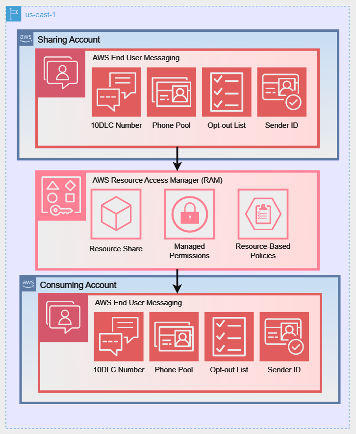
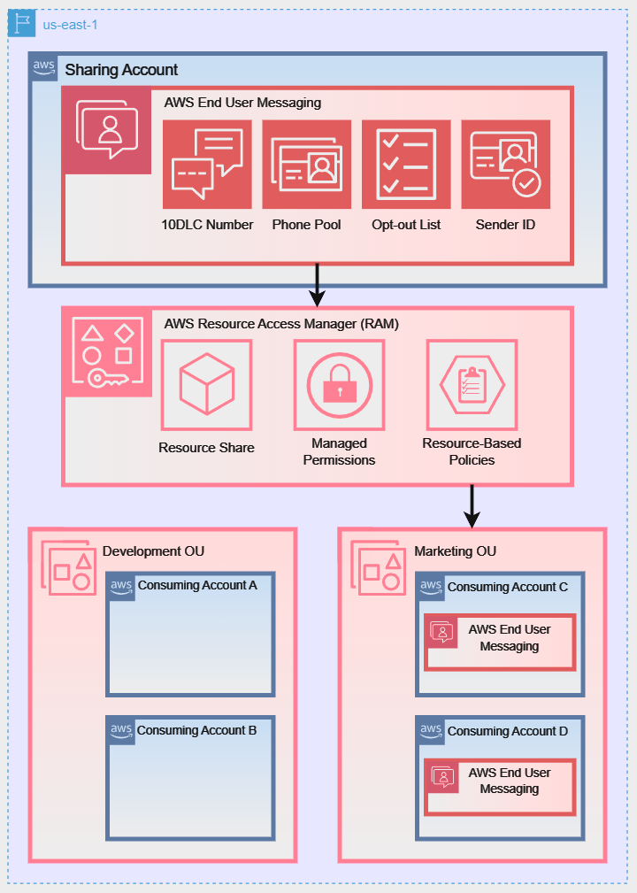
To better illustrate these sharing models, the following diagrams show how a Sharing Account can share its AWS End User Messaging resources using different strategies:

Diagram 1: Direct Account-to-Account Sharing:

Diagram 2: Sharing with an Entire AWS Organization:

Diagram 3: Sharing with a Specific Organizational Unit (OU):

Prerequisites and Setup

For the following walkthrough, we will demonstrate how to configure the setup for Diagram 1: Direct Account-to-Account Sharing. However, the steps for managing and using the resource share are similar for all three scenarios. Before you begin, ensure your environment is set up correctly.

Note for AWS Organizations Users: When your account is managed by AWS Organizations, you can take advantage of that to share resources more easily. With or without Organizations, a user can share with individual accounts. However, if your account is in an organization, then you can share with individual accounts, or with all accounts in the organization or in an OU without having to enumerate each account.

If you plan to share resources using AWS Organizations (as shown in Diagram 2 or Diagram 3), you must complete the following prerequisite steps from your organization’s management account before creating a resource share:

1. Enable all features in your organization:

aws organizations enable-all-features

2. Enable resource sharing with AWS RAM: This creates the necessary service-linked role.

aws ram enable-sharing-with-aws-organization

1. Required IAM Permissions

The IAM user or role performing these actions needs permissions for both AWS RAM and AWS End User Messaging. The following policy grants the necessary permissions to manage resource shares.

{
    "Version": "2012-10-17",
    "Statement": [
        {
            "Sid": "RAMResourceShareManagement",
            "Effect": "Allow",
            "Action": [
                "ram:UpdateResourceShare",
                "ram:DeleteResourceShare",
                "ram:AssociateResourceShare",
                "ram:DisassociateResourceShare"
            ],
            "Resource": "arn:aws:ram:*:*:resource-share/*"
        },
        {
            "Sid": "DiscoveryAndCreationPermissions",
            "Effect": "Allow",
            "Action": [
                "ram:CreateResourceShare",
                "ram:GetResourceShares",
                "ram:ListResources",
                "organizations:ListAccounts",
                "organizations:DescribeOrganization",
                "pinpoint-sms-voice-v2:DescribePhoneNumbers",
                "pinpoint-sms-voice-v2:DescribeSenderIds",
                "pinpoint-sms-voice-v2:DescribeOptOutLists",
                "pinpoint-sms-voice-v2:DescribePools"
            ],
            "Resource": "*"
        }
    ]
}

Note on Least Privilege: This policy follows the security best practice of granting least privilege. The first statement scopes modification permissions to only AWS RAM resource shares. The second statement grants permissions for discovery actions (like Describe* and List*) and the ram:CreateResourceShare action, which require "Resource": "*" as they do not operate on a specific, pre-existing resource.

2. Regionality Requirement

Important Reminder: resource sharing with AWS RAM is a regional feature. You can only share resources with accounts within the same AWS Region where those resources are located.

For example, a resource in us-east-1 can only be shared with other accounts in us-east-1, regardless of where those accounts operate other resources. Ensure that the resources you intend to share and the accounts that you anticipate sharing with are each considering the same Region for this process.

Creating and Managing Resource Shares (Sharing Account Actions)

This section provides a step-by-step guide to sharing your resources using the AWS CLI. We will walk through creating a resource share, associating and disassociating resources, and checking the status of your shares.

Step 1: Create an Empty Resource Share

First, create the resource share. Think of this as an empty container. You will associate principals (the consuming accounts) and resources (the phone numbers, etc.) with this share.

In the command below, we will create a share named EUM-Shared-Resources for an external account.

# Create a resource share and grant default End User Messaging permissions # Replace 123456789012 with the consuming account's ID
aws ram create-resource-share \
    --name "EUM-Shared-Resources" \
    --principals "123456789012" \
    --permission-arns "arn:aws:ram::aws:permission/AWSRAMDefaultPermissionSmsVoice" \
    --allow-external-principals \
    --region us-east-1
  • --principals: Specify one or more AWS account IDs.
  • --allow-external-principals: This flag is required when sharing with accounts that are not part of your AWS Organization.

Expected Response: A successful command returns a JSON object describing the new resource share. Note that allowExternalPrincipals is now true.

{
    "resourceShare": {
        "resourceShareArn": "arn:aws:ram:us-east-1:111122223333:resource-share/a1b2c3d4-5678-90ab-cdef-example11111",
        "name": "EUM-Shared-Resources",
        "owningAccountId": "111122223333",
        "allowExternalPrincipals": false,
        "status": "ACTIVE",
        "tags": [],
        "featureSet": "STANDARD"
    }
}

For the following sections and when specifying resource ARNs, ensure you’re using the correct format for AWS End User Messaging resources:

  • Phone numbers: arn:aws:sms-voice:region:account-id:phone-number/phonenumber-id
  • Sender IDs: arn:aws:sms-voice:region:account-id:sender-id/senderid
  • Opt-out lists: arn:aws:sms-voice:region:account-id:opt-out-list/optoutlist-id
  • Pools: arn:aws:sms-voice:region:account-id:pool/pool-id

Replace ‘region‘, ‘account-id‘, and the specific resource IDs with your actual values.

Step 2: Associate Resources with the Share

Now that you have your “container,” you can add resources to it. The associate-resource-share command links one or more of your End User Messaging resources to the share you just created, making them available to the principals.

# Define the ARN of the resource share from the previous step
RESOURCE_SHARE_ARN="arn:aws:ram:us-east-1:111122223333:resource-share/a1b2c3d4-5678-90ab-cdef-111111111111"

# Associate a phone number and a pool with the share # Replace the resource-arns with your actual resource ARNs
aws ram associate-resource-share \
    --resource-share-arn "$RESOURCE_SHARE_ARN" \
    --resource-arns \
        "arn:aws:sms-voice:us-east-1:111122223333:phone-number/phonenumber-a1b2c3d4" \
        "arn:aws:sms-voice:us-east-1:111122223333:pool/pool-b2c3d4e5" \
    --region us-east-1

Expected Response: A successful association returns a JSON object confirming the association and showing its status. The status will initially be ASSOCIATING and will transition to ASSOCIATED once complete.

Note: The association process is asynchronous. We’ll show you how to verify the completion status in the next step using the get-resource-shares and list-resources commands. It’s important to confirm the status has changed to ASSOCIATED before attempting to use the shared resources.

Step 3: Verify the Status and contents of the Share

Before making changes, it’s good practice to verify what’s in the share. Use get-resource-shares to check the status and list-resources to see the contents. This process helps ensure that all intended resources are properly associated and accessible to the principals you’ve designated.

# Verify the association status is ASSOCIATED
aws ram get-resource-shares \
    --resource-owner SELF \
    --name "EUM-Shared-Resources" \
    --association-status ASSOCIATED \
    --region us-east-1

Expected Response: If the command returns no results, wait a few moments and try again. The association process is typically quick but can sometimes take up to a few minutes.

{
    "resourceShares": [
        {
            "resourceShareArn": "arn:aws:ram:us-east-1:111122223333:resource-share/12345678-abcd-1234-efgh-111122223333",
            "name": "EUM-Shared-Resources",
            "owningAccountId": "111122223333",
            "allowExternalPrincipals": true,
            "status": "ACTIVE",
            "creationTime": "2023-07-01T12:00:00.000Z",
            "lastUpdatedTime": "2023-07-01T12:00:00.000Z",
            "featureSet": "STANDARD"
        }
    ]
}

Review the output carefully to ensure all intended resources are listed. If any resources are missing, you may need to reassociate them using the associate-resource-share command.

Expected Response (list-resources): This command will return a list of JSON objects, each representing a resource in the share.

# List the ARNs of all resources currently in the share
aws ram list-resources \
    --resource-owner SELF \
    --resource-share-arns "$RESOURCE_SHARE_ARN" \
    --region us-east-1

Review the output carefully to ensure all intended resources are listed. If any resources are missing, you may need to reassociate them using the associate-resource-share command.

# List the ARNs of all resources currently in the share
aws ram list-resources \
    --resource-owner SELF \
    --resource-share-arns "$RESOURCE_SHARE_ARN" \
    --region us-east-1

Expected Response (list-resources): This command will return a list of JSON objects, each representing a resource in the share.

{
    "resources": [
        {
            "arn": "arn:aws:sms-voice:us-east-1:111122223333:phone-number/phonenumber-a1b2c3d4",
            "type": "sms-voice:PhoneNumber",
            "resourceShareArn": "arn:aws:ram:us-east-1:111122223333:resource-share/a1b2c3d4-5678-90ab-cdef-example11111",
            "status": "AVAILABLE"
        },
        {
            "arn": "arn:aws:sms-voice:us-east-1:111122223333:pool/pool-b2c3d4e5",
            "type": "sms-voice:Pool",
            "resourceShareArn": "arn:aws:ram:us-east-1:111122223333:resource-share/a1b2c3d4-5678-90ab-cdef-example11111",
            "status": "AVAILABLE"
        }
    ]
}

Step 4: Disassociate Specific Resources from the Share

To stop sharing a specific resource, you use the disassociate-resource-share command. You must provide the ARN of the resource you wish to remove. This gives you granular control, allowing you to remove one resource while continuing to share others.

# Disassociate only the phone number from the share
aws ram disassociate-resource-share \
    --resource-share-arn "$RESOURCE_SHARE_ARN" \
    --resource-arns "arn:aws:sms-voice:us-east-1:111122223333:phone-number/phonenumber-a1b2c3d4" \
    --region us-east-1

Expected Response: The response will be nearly identical to the associate response, confirming the disassociation request. The status will be DISASSOCIATING.

{
    "resourceShareAssociations": [
        {
            "resourceShareArn": "arn:aws:ram:us-east-1:111122223333:resource-share/a1b2c3d4-5678-90ab-cdef-example11111",
            "associatedEntity": "arn:aws:sms-voice:us-east-1:111122223333:phone-number/phonenumber-a1b2c3d4",
            "associationType": "RESOURCE",
            "status": "DISASSOCIATING",
            "external": false
        }
    ]
}

How to Use Shared Resources

Once resources are shared, users in the consuming accounts can discover and use them for sending messages.

Step 1: Discovering Shared Resources

From a consuming account, you can list resources that have been shared with you by using the --filters parameter in the describe-* commands.

Note: Shared resources are discoverable via the AWS CLI and SDKs but will not appear in the AWS Management Console of the consuming account. This is expected behavior, as the resources are owned by the sharing account.

# List phone numbers shared with your account
aws pinpoint-sms-voice-v2 describe-phone-numbers \
    --filters Name=shared-with-me,Values=true \
    --region us-east-1
# List sender IDs shared with your account
aws pinpoint-sms-voice-v2 describe-sender-ids \
--filters Name=shared-with-me,Values=true \
--region us-east-1

# List pools shared with your account
aws pinpoint-sms-voice-v2 describe-pools \
--filters Name=shared-with-me,Values=true \
--region us-east-1

# List shared opt-out lists with region specification
aws pinpoint-sms-voice-v2 describe-opt-out-lists \
--filters Name=shared-with-me,Values=true \
--region us-east-1

Expected Response: The command returns a JSON object listing the shared resources, including their ARNs, which you will need for sending messages.

{
    "PhoneNumbers": [
        {
            "PhoneNumberArn": "arn:aws:sms-voice:us-east-1:111122223333:phone-number/phonenumber-a1b2c3d4",
            "PhoneNumberId": "phonenumber-a1b2c3d4",
            "PhoneNumber": "+12065550100",
            "Status": "ACTIVE",
            "MessageType": "TRANSACTIONAL",
            "TwoWayEnabled": true,
            "CreatedTimestamp": "2023-10-26T14:34:56.123Z"
        }
    ]
}

Step 2: Sending Messages with Shared Resources

Important: When using shared resources, consuming accounts must specify the full ARN of the shared resource in API calls. This differs from resource owners, who can use either the resource ID, ARN, or the number directly. You can specify the ARN of an individual phone number or a pool as the origination-identity.

# Send an SMS using a shared Phone Number ARN (consuming account MUST use ARN)
aws pinpoint-sms-voice-v2 send-text-message \
    --destination-phone-number "+12065550199" \
    --origination-identity "arn:aws:sms-voice:us-east-1:111122223333:phone-number/phonenumber-a1b2c3d4" \
    --message-body "Hello from a shared number!" \
    --region us-east-1

# Send an SMS using a shared Pool ARN (consuming account MUST use ARN)
aws pinpoint-sms-voice-v2 send-text-message \
    --destination-phone-number "+12065550199" \
    --origination-identity "arn:aws:sms-voice:us-east-1:111122223333:pool/pool-b2c3d4e5" \
    --message-body "Hello from a shared pool!" \
    --region us-east-1

Expected Response: A successful send-text-message call will return a MessageId, which confirms that the service has accepted the message for delivery.

{
    "MessageId": "a1b2c3d4-5678-90ab-cdef-example22222"
}

Message Delivery Reporting:

Once a message is sent, understanding its delivery status is crucial for ensuring your communications are effective. AWS End User Messaging provides several mechanisms for tracking message delivery, giving you a multi-layered approach to reporting.

Delivery Receipts (DLRs):

For traditional, carrier-provided Delivery Receipts (DLRs), which can sometimes take up to 72 hours to be returned, you must configure an event destination. This is the most common method for confirming that a message has reached the recipient’s handset, and is achieved through a Configuration Set.

For shared resources:

  • The configuration set must be created and managed in the sharing account.
  • The consuming account must then reference the ARN of the configuration set when sending messages.
# Example for consuming account
aws pinpoint-sms-voice-v2 send-text-message 
    --destination-phone-number "+12065550199" 
    --origination-identity "arn:aws:sms-voice:us-east-1:111122223333:phone-number/phonenumber-a1b2c3d4" 
    --message-body "Hello from a shared number!" 
    --configuration-set-name "arn:aws:sms-voice:us-east-1:111122223333:configuration-set/MyConfigSet" 
    --region us-east-1

For a detailed walkthrough, see our companion blog post, How to Send SMS Using Configuration Sets with AWS End User Messaging.

Message Feedback:

For more immediate, application-driven insights, you can use the Message Feedback feature. This allows you to programmatically mark messages as “delivered” based on a user’s action, such as using a one-time password (OTP) or clicking a link in the message. This provides a real-time confirmation loop that is independent of carrier DLRs.

Amazon CloudWatch:

To monitor these events at scale, you can stream them to Amazon CloudWatch Logs to track key performance indicators like the number of messages sent and delivered, and to set up alerts based on your specific business needs.

To set up comprehensive reporting:

  1. Configure an event destination for DLRs and detailed status events.
  2. Set up CloudWatch dashboards and alerts for ongoing monitoring.

This multi-layered approach provides both immediate feedback and long-term delivery insights, allowing you to optimize your messaging strategy and quickly identify potential delivery issues.

Troubleshooting Common Issues

  • Permission Denied Errors: If a consuming account cannot access a shared resource, verify that the consuming account’s IAM policies include the necessary permissions. Here’s an example policy:
{
    "Version": "2012-10-17",
    "Statement": [
        {
            "Effect": "Allow",
            "Action": [
                "pinpoint-sms-voice-v2:SendTextMessage",
                "pinpoint-sms-voice-v2:SendVoiceMessage",
                "pinpoint-sms-voice-v2:DescribePhoneNumbers",
                "pinpoint-sms-voice-v2:DescribeSenderIds",
                "pinpoint-sms-voice-v2:DescribeOptOutLists",
                "pinpoint-sms-voice-v2:DescribePools"
            ],
            "Resource": "*"
        }
    ]
}
  • Resource Not Visible: Remember that shared resources do not appear in the consuming account’s AWS Management Console. If the describe-* commands with the shared-with-me filter return no results, ensure the resource share status is ACTIVE in the sharing account.
    • If sharing via AWS Organizations, confirm the consuming account is correctly placed in the specified OU. You can find more information on managing OUs in the AWS Organizations User Guide.
  • CLI Command Fails: If a command fails with a “not found” or “invalid parameter” error, it is often due to an incorrect ARN. Double-check that the ARNs for resources, principals, and the resource share itself are correct. A Permission Denied error, on the other hand, points to an IAM policy issue..

Best Practices and Considerations

  • Security: Always follow the principle of least privilege. Use AWS managed permissions like AWSRAMDefaultPermissionSmsVoice where possible and create customer-managed permissions only for specific, granular requirements.
  • Cost: The sharing account is billed for provisioning the resources (e.g., the monthly cost of a phone number). Consuming accounts are billed for their usage of those shared resources (e.g., the cost per message sent). There are no additional costs for using AWS RAM.
  • Throughput and Quotas: Resource throughput quotas (e.g., messages per second) are shared along with the resource. High volume sending from multiple consuming accounts using the same shared number or pool, could collectively hit the service quota, which may result in throttling. Plan your usage accordingly or request quota increases if necessary.

Conclusion

This guide has equipped you to centralize your AWS End User Messaging resources using AWS Resource Access Manager. By implementing this strategy, you can directly address the common challenges of a multi-account environment: maintaining consistent branding with shared Sender IDs, ensuring comprehensive compliance with centralized opt-out lists, and reducing operational overhead by managing resources in one place.

We have walked through the entire lifecycle, from the initial prerequisites in AWS Organizations and IAM, to the step-by-step CLI commands for creating shares, associating resources, and enabling consuming accounts to use them. By applying these techniques and keeping the best practices for security and throughput in mind, you are now able to build a more efficient, secure, and scalable communication platform across your entire AWS ecosystem.
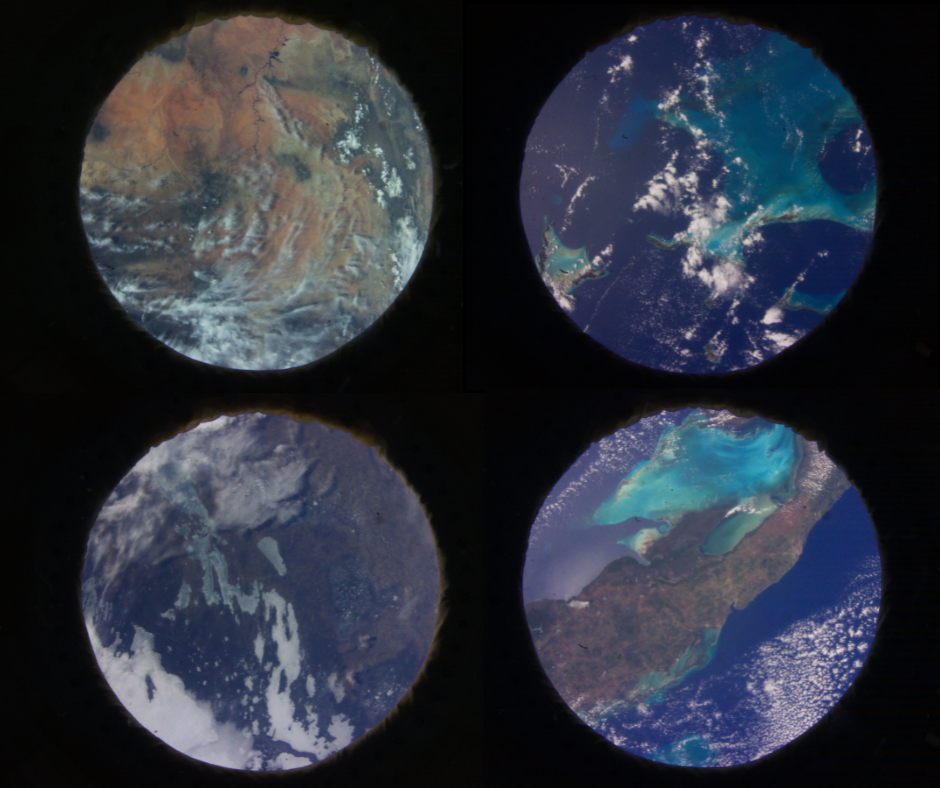
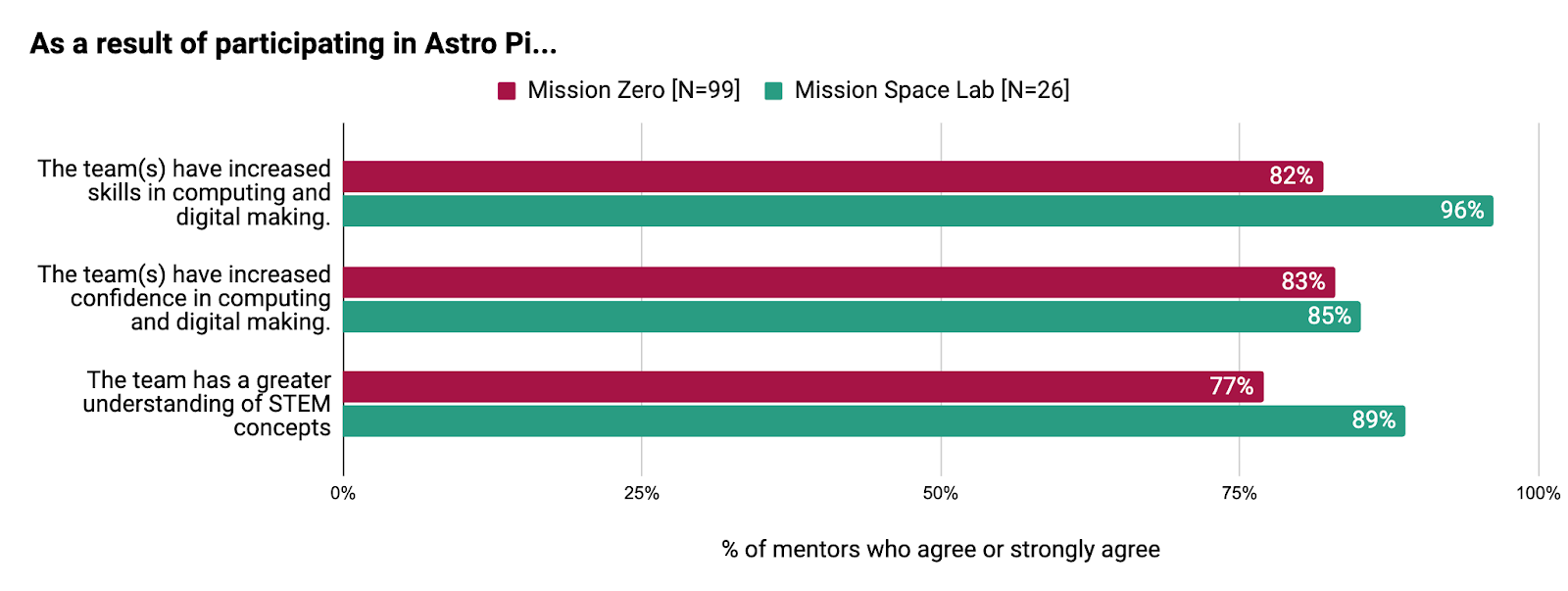
Adding stubble to Ubuntu’s generic Arm64 Desktop ISOs

Post Syndicated from jzb original https://lwn.net/Articles/1034579/

Tobias Heider has written
an article that explains changes that are coming for Ubuntu’s generic
Arm64 desktop ISO images in the 25.10 release. The current solution,
Heider says, depends on GRUB features that are unavailable in secure
boot mode and require adding device-specific logic to multiple
packages. The new solution, called stubble,
is derived from systemd-stub:

A bundled stubble image contains stubble itself, a Linux kernel, a
HWID lookup table to map devices to device trees and multiple device
trees. When grub loads this “kernel”, stubble executes first, reads
the SMBIOS table to generate HWIDs, looks for a match in the embeeded
lookup table and loads a matching device tree before passing control
to the actual Linux kernel.

The elegance in this approach lies in how it interacts with the
rest of the system. Integrating stubble happens entirely at build time
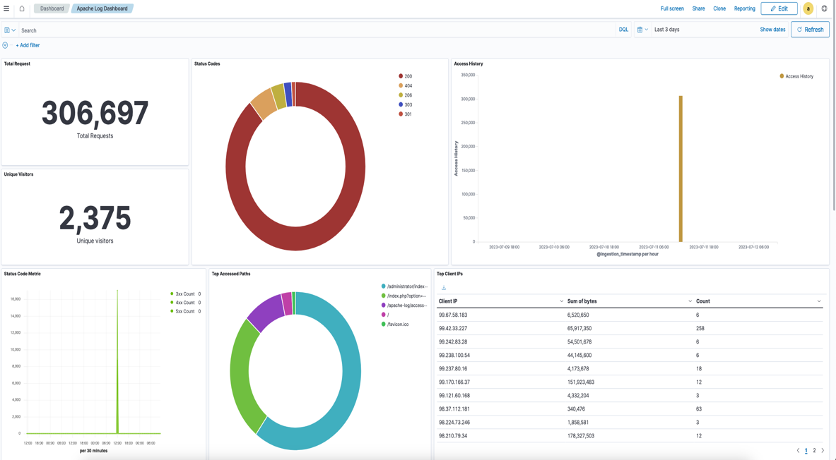
in the kernel package. The stubble package is a build dependency for
the kernel. After building the kernel itself, we bundle it with
stubble and our DTBs and ship the combined binary instead. The
resulting stubble + kernel + dtb bundle can be loaded by grub like any
other Ubuntu kernel. No further changes in grub or other packages are
necessary to make it work.

[$] Python, tail calls, and performance

Post Syndicated from jake original https://lwn.net/Articles/1033373/

Ken Jin welcomed EuroPython 2025 attendees to
his talk entitled “Building a new tail-calling interpreter for Python”, but
noted that the title really should be: “Measuring the performance of
compilers and interpreters is really hard”. Jin’s efforts to switch the CPython interpreter to use tail calls,
which can be optimized as regular jumps,
initially seemed to produce an almost miraculous performance improvement.
As his modified title suggests, the actual improvement
was rather smaller
; there is still some performance improvement and
there are other benefits from the change.

How we built AI face cropping for Images

Post Syndicated from Deanna Lam original https://blog.cloudflare.com/ai-face-cropping-for-images/

During Developer Week 2024, we introduced AI face cropping in private beta. This feature automatically crops images around detected faces, and marks the first release in our upcoming suite of AI image manipulation capabilities.

AI face cropping is now available in Images for everyone. To bring this feature to general availability, we moved our CPU-based prototype to a GPU-based implementation in Workers AI, enabling us to address a number of technical challenges, including memory leaks that could hamper large-scale use.


Photograph by Suad Kamardeen (@suadkamardeen) on Unsplash

Turning raw images into production-ready assets

We developed face cropping with two particular use cases in mind:

Social media platforms and AI chatbots. We observed a lot of traffic from customers who use Images to turn unedited images of people into smaller profile pictures in neat, fixed shapes.

E-commerce platforms. The same product photo might appear in a grid of thumbnails on a gallery page, then again on an individual product page with a larger view. The following example illustrates how cropping can change the emphasis from the model’s shirt to their sunglasses.


Photograph by Media Modifier (@mediamodifier) on Unsplash

When handling high volumes of media content, preparing images for production can be tedious. With Images, you don’t need to manually generate and store multiple versions of the same image. Instead, we serve copies of each image, each optimized to your specifications, while you continue to store only the original image.

Crop everything, everywhere, all at once

Cloudflare provides a library of parameters to manipulate how an image is served to the end user. For example, you can crop an image to a square by setting its width and height dimensions to 100×100.

By default, images are cropped toward the center coordinates of the original image. The gravity parameter can affect how an image gets cropped by changing its focal point. You can specify coordinates to use as the focal point of an image or allow Cloudflare to automatically determine a new focal point.


The gravity parameter is useful when cropping images with off-centered subjects. Photograph by Andrew Small (@andsmall) on Unsplash

The gravity=auto option uses a saliency algorithm to pick the most optimal focal point of an image. Saliency detection identifies the parts of an image that are most visually important; the cropping operation is then applied toward this region of interest. Our algorithm analyzes images using visual cues such as color, luminance, and texture, but doesn’t consider context within an image. While this setting works well on images with inanimate objects like plants and skyscrapers, it doesn’t reliably account for subjects as contextually meaningful as people’s faces.

And yet, images of people comprise the majority of bandwidth usage for many applications, such as an AI chatbot platform that uses Images to serve over 45 million unique transformations each month. This presented an opportunity for us to improve how developers can optimize images of people.

AI face cropping can be performed by using the gravity=face option, which automatically detects which pixels represent the face (or faces) and uses this information to crop the image. You can also affect how closely the image is cropped toward the face; the zoom parameter controls the threshold for how much of the surrounding area around the face will be included in the image.

We carefully designed our model pipeline with privacy and confidentiality top of mind. This feature doesn’t support facial identification or recognition. In other words, when you optimize with Cloudflare, we’ll never know that two different images depict the same person, or identify the specific people in a given image. Instead, AI face cropping with Images is intentionally limited to face detection, or identifying the pixels that represent a human face.

From pixels to people

Our first step was to select an open-source model that met our requirements. Behind the scenes, our AI face cropping uses RetinaFace, a convolutional neural network model that classifies images with human faces.

A neural network is a type of machine learning process that loosely resembles how the human brain works. A basic neural network has three parts: an input layer, one or more hidden layers, and an output layer. Nodes in each layer form an interconnected network to transmit and process data, where each input node is connected to nodes in the next layer.


A fully connected layer passes data from one layer to the next.

Data enters through the input layer, where it is analyzed before being passed to the first hidden layer. All of the computation is done in the hidden layers, where a result is eventually delivered through the output layer.

A convolutional neural network (CNN) mirrors how humans look at things. When we look at other people, we start with abstract features, like the outline of their body, before we process specific features, like the color of their eyes or the shape of their lips.

Similarly, a CNN processes an image piece-by-piece before delivering the final result. Earlier layers look for abstract features like edges and colors and lines; subsequent layers become more complex and are each responsible for identifying the various features that comprise a human face. The last fully connected layer combines all categorized features to produce one final classification of the entire image. In other words, if an image contains all of the individual features that define a human face (e.g. eyes, nose), then the CNN concludes that the image contains a human face.

We needed a model that could determine whether an image depicts a person (image classification), as well as exactly where they are in the image (object detection). When selecting a model, some factors we considered were:

  • Performance on the WIDERFACE dataset. This is the state-of-the-art face detection benchmark dataset, which contains 32,203 images of 393,703 labeled faces with a high degree of variability in scale, pose, and occlusion.

  • Speed (in frames per second). Most of our image optimization requests occur on delivery (rather than before an image gets uploaded to storage), so we prioritized performance for end-user delivery.

  • Model size. Smaller model sizes run more efficiently.

  • Quality. The performance boost from smaller models often gets traded for the quality—the key is balancing speed with results.

Our initial test sample contained 500 images with varying factors like the number of faces in the image, face size, lighting, sharpness, and angle. We tested various models, including BlazeFast, R-CNN (and its successors Fast R-CNN and Faster R-CNN), RetinaFace, and YOLO (You Only Look Once).

Two-stage detectors like BlazeFast and R-CNN propose potential object locations in an image, then identify objects in those regions of interest. One-stage detectors like RetinaFace and YOLO predict object locations and classes in a single pass. In our research, we observed that two-stage detector methods provided higher accuracy, but performed too slowly to be practical for real traffic. On the other hand, one-stage detector methods were efficient and performant while still highly accurate.

Ultimately, we selected RetinaFace, which showed the highest precision of 99.4% and performed faster than other models with comparable values. We found that RetinaFace delivered strong results even with images containing multiple blurry faces:


Photograph by Anne Nygård (@polarmermaid) on Unsplash

Inference—the process of using training models to make decisions—can be computationally demanding, especially with very large images. To maintain efficiency, we set a maximum size limit of 1024×1024 pixels when sending images to the model.

We pass images within these dimensions directly to the model for analysis. But if either width or height dimension exceeds 1024 pixels, then we instead create an inference image to send to the model; this is a smaller copy that retains the same aspect ratio as the original image and does not exceed 1024 pixels in either dimension. For example, a 125×2000 image will be downscaled to 64×1024. Creating this resized, temporary version reduces the amount of data that the model needs to analyze, enabling faster processing.

The model draws all of the bounding boxes, or the regions within an image that define the detected faces. From there, we construct a new, outer bounding box that encompasses all of the individual boxes, calculating its top-left and bottom-right points based on the boxes that are closest to the top, left, bottom, and right edges of the image.

The top-left point uses the x coordinate from the left-most box and the y coordinate from the top-most box. Similarly, the bottom-right point uses the x coordinate from the right-most box and the y coordinate from the bottom-most box. These coordinates can be taken from the same bounding boxes; if a single box is closest to both the top and left edges, then we would use its top-left corner as the top-left point of the outer bounding box.


AI face cropping identifies regions that represent faces, then determines an outer bounding box and focal point based on the top-most, left-most, right-most, and bottom-most bounding boxes.

Once we define the outer bounding box, we use its center coordinates as the focal point when cropping the image. From our experiments, we found that this produced better and more balanced results for images with multiple faces compared to other methods, like establishing the new focal point around the largest detected face.

The cropped image area is calculated based on the dimensions of the outer bounding box (“d”) and a specified zoom level (“z”) in the formula (1 ÷ z) × d. The zoom parameter accepts floating points between 0 and 1, where we crop the image to the bounding box when zoom=1 and include more of the area around the box as zoom trends toward 0.

Consider an original image that is 2048×2048. First, we create an inference image that is 1024×1024 to meet our size limits for face detection. Second, we define the outer bounding box using the model’s predictions—we’ll use 100×500 for this example. At zoom=0.5, our formula generates a crop area that is twice as large as the bounding box, with new width (“w”) and height (“h”) dimensions of 200×1000:


We also apply a min function that chooses the smaller number between the input dimensions and the calculated dimensions, ensuring that the new width and height never exceed the dimensions of the image itself. In other words, if you try to zoom out too much, then we use the full width or height of the image instead of defining a crop area that will extend beyond the edge of the image. For example, at zoom=0.25, our formula yields an initial crop area of 400×2000. Here, since the calculated height (2000) is larger than the input height (1024), we use the input height to set the crop area to 400×1024.

Finally, we need to scale the crop area back to the size of the original image. This applies only when a smaller inference image is created.

We initially downscaled the original 2048×2048 image by a factor of 2 to create the 1024×1024 inference image. This means that we need to multiply the dimensions of the crop area—400×1024 in our latest example—by 2 to produce our final result: a cropped image that is 800×2048.

The architecture behind the earliest build

In the beta version, we rewrote the model using TensorFlow Rust to make it compatible with our existing Rust-based stack. All of the computations for inference—where the model classifies and locates human faces—were executed on CPUs within our network.

Initially, this worked well and we saw near-realtime results.

However, the underlying limitations of our implementation became apparent when we started receiving consistent alerts that our underlying Images service was nearing its limits for memory usage. The increased memory usage didn’t line up with any recent deployments around this time, but a hunch led us to discover that the face cropping compute time graph had an uptick that matched the uptick in memory usage. Further tracing confirmed that AI face cropping was at the root of the problem.
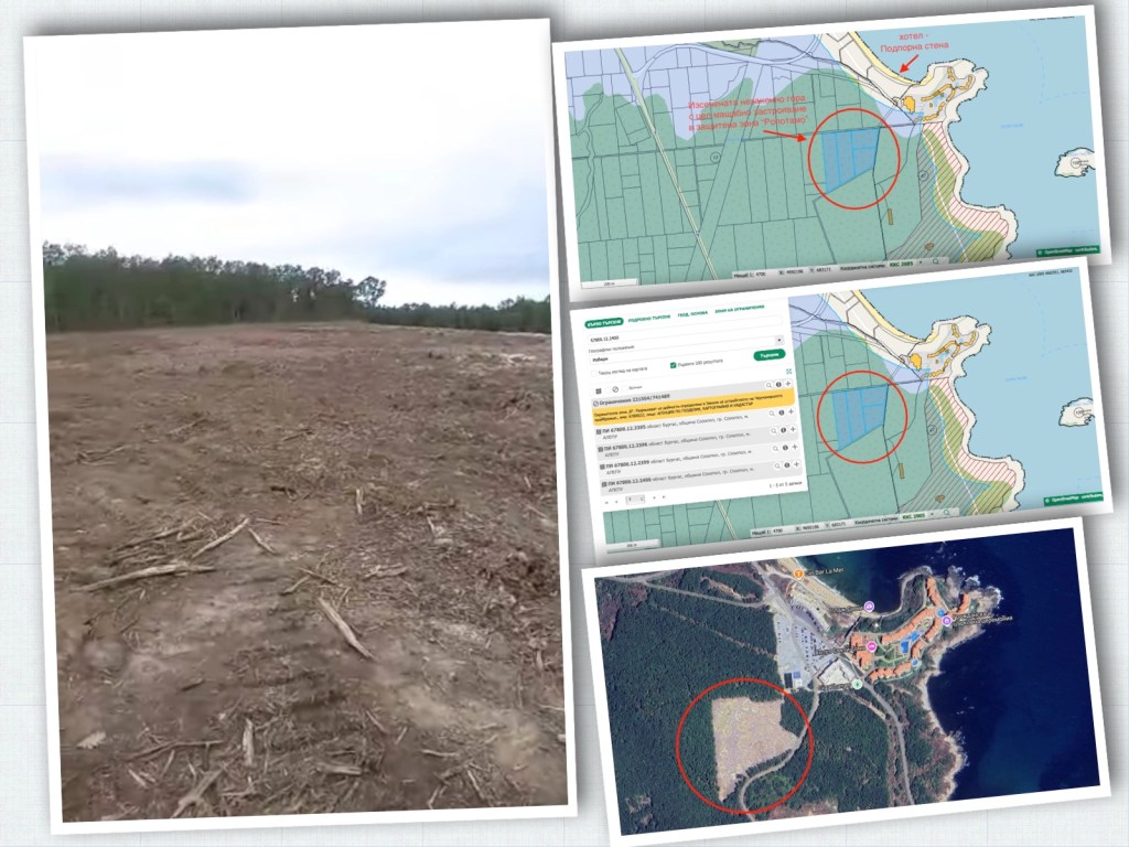
When a service runs out of memory, it terminates its processes to free up memory and prevent the system from crashing. Since CPU-based implementations share RAM with other processes, this can potentially cause errors for other image optimization operations. In response, we switched our memory allocator from glibc malloc to jemalloc. This allowed us to use less memory at runtime, saving about 20 TiB of RAM globally. We also started culling the number of face cropping requests to limit CPU usage.
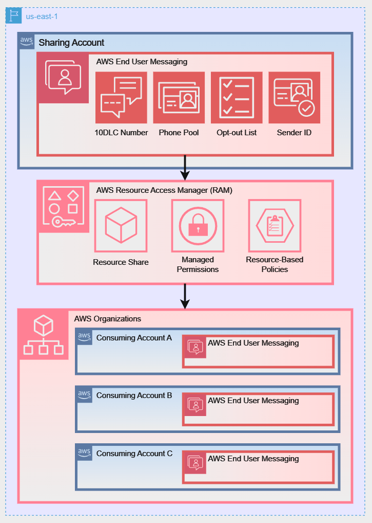
At this point, AI face cropping was already limited to our own internal uses and a small number of beta customers. These steps only temporarily reduced our memory consumption. They weren’t sufficient for handling global traffic, so we looked toward a more scalable design for long-term use.

Doing more with less (memory)

With memory usage alerts looming in the distance, it became clear that we needed to move to a GPU-based approach.

Unlike with CPUs, a GPU-based implementation avoids contention with other processes because memory access is typically dedicated and managed more tightly. We partnered with the Workers AI team, who created a framework for internal teams to integrate payloads into their model catalog for GPU access.

Some Workers AI models have their own standalone containers; this isn’t practical for every model, as routing traffic to multiple containers can be expensive. When using a GPU through Workers AI, the data needs to travel over the network, which can introduce latency. This is where model size is especially relevant, as network transport overhead becomes more noticeable with larger models.

To address this, Workers AI wraps smaller models in a single container and utilizes a latency-sensitive routing algorithm to identify the best instance to serve each payload. This means that models can be offloaded when there is no traffic.


A scheduler is used to optimize how—and when—models in the same container interact with GPUs.

RetinaFace runs on 1 GB of VRAM on the smallest GPU; it’s small enough that it can be hot swapped at runtime alongside similarly sized models. If there is a call for the RetinaFace model, then the Python code will be loaded into the environment and executed.

As expected, we saw a significant drop in memory usage after we moved the feature to Workers AI. Now, each instance of our Images service consumes about 150 MiB of memory.


With this new approach, memory leaks pose less concern to the overall availability of our service. Workers AI executes models within containers, so they can be terminated and restarted as needed without impacting other processes. Since face cropping runs separately from our Images service, restarting it won’t halt our other image optimization operations.

Applying AI face cropping to our blog

As part of our beta launch, we updated the Cloudflare blog to apply AI face cropping on author images.

Authors can submit their own images, which appear as circular profile pictures in both the main blog feed and individual blog posts. By default, CSS centers images within their containers, making off-centered head positions more obvious. When two profile pictures include different amounts of negative space, this can also lead to a visual imbalance where authors’ faces appear at different scales:


AI face cropping makes posts with multiple authors appear more balanced.

In the example above, Austin’s original image is cropped tightly around his face. On the other hand, Taylor’s original image includes his torso and a larger margin of the background. As a result, Austin’s face appears larger and closer to the center than Taylor’s does. After we applied AI face cropping to profile pictures on the blog, their faces appear more similar in size, creating more balance and cohesion on their co-authored post.

A new era of image editing, now in Images

Many developers already use Images to build scalable media pipelines. Our goal is to accelerate image workflows by automating rote, manual tasks.

For the Images team, this is only the beginning. We plan to release new AI capabilities, including features like background removal and generative upscale. You can try AI face cropping for free by enabling transformations in the Images dashboard.

The collective thoughts of the interwebz