Version
2026.05 of the Buildroot tool
has been released. Buildroot simplifies and automates the process of
building embedded Linux systems using cross-compilation. Notable
changes in this release include support for Arm Neoverse cores,
addition of XFS rootfs generation, as well as many package updates and
bug fixes. See the CHANGES
file for the full list.
For most of the Internet’s history, public and private infrastructure operated as separate worlds. Public applications lived behind content delivery networks (CDNs) and web application firewalls (WAFs). Private applications lived behind virtual private networks (VPNs), firewalls, and separate operational stacks. We think that distinction is becoming obsolete.
Many of the applications organizations care about are not public websites. They are internal APIs, AI agent backends, MCP servers, operational tools, and services that were never designed to be exposed to the public Internet. Yet these applications still need modern security, performance, and programmability services. Security should be a property of the traffic reaching an application, not an accident of where the application happens to sit.
Until now, applying those services to private applications often required public IPs, firewall exceptions, connector software, or complex networking. As a result, many private applications missed out on capabilities such as WAF, bot management, rate limiting, caching, traffic acceleration, rewrites, and Workers, despite needing the same protections and controls as public-facing applications.
Today, we’re launching Application Services for Private Origins in closed beta for eligible Enterprise customers. Customers can now securely route traffic to private origins without exposing those origins to the public Internet. This allows Cloudflare’s security, performance, and programmability services to protect applications running on private networks, just as they do for public Internet applications.
WAF rules, bot management, rate limiting, caching, rewrites, and Workers can now sit in front of private origins without requiring public IP exposure, inbound firewall rules, or cloudflared running on the origin.
Four use cases, one application layer
This routing model builds on connectivity patterns Cloudflare already supports today through Cloudflare Tunnel, Cloudflare One Client, and private network integrations. For years, Cloudflare Tunnel has allowed customers to route public traffic to private applications through cloudflared. This new capability extends the same model to existing Cloudflare WAN or Cloudflare Mesh connectivity without requiring connector software running on the origin.
Much of that connectivity is orchestrated through Cloudflare’s private networking routing layer that determines how traffic reaches private destinations across Cloudflare Tunnels, Virtual Networks, Cloudflare Mesh, and other connectivity models. Customers can define their routing behavior through APIs and the dashboard instead of managing separate networking stacks for each product.
We have extended Cloudflare’s private networking layer directly into the application services stack, allowing security and performance proxy infrastructure to treat private IPs as valid origin targets for public hostnames. As a result, the same private IPs previously reachable only through Cloudflare Tunnel, Cloudflare One, Cloudflare Mesh, or Cloudflare WAN can now sit behind Cloudflare’s security, performance, and programmability services the same way public origins already do.
This also creates a more unified model across Cloudflare products. Workers VPC bindings and Spectrum private origin routing now rely on the same underlying private connectivity layer, giving customers a single source of truth for controlling how private traffic moves through their Cloudflare environment.
Application traffic now falls into four combinations based on where users come from and where applications live:
The combination on the upper right is what Cloudflare has always done: users on the Internet reach applications on the Internet, with Cloudflare in the middle. The bottom right is Cloudflare One: users on private networks reach public services securely.
The upper left is what we are shipping today. The bottom left, private-to-private, is what we are building toward next.
What is shipping today
Until now, getting public traffic to a private origin often meant making tradeoffs. Customers could use Cloudflare Tunnel, which runs cloudflared, our connector software, on or near the origin, or Cloudflare Load Balancing with private origin pools for health checks and failover. In many cases, organizations also maintained parallel infrastructure such as public-facing load balancers, reverse proxies, mTLS between hops, and TLS termination across multiple layers. As a result, applying Cloudflare’s full Application Services stack to private applications often required additional complexity, operational overhead, or separate products. Application Services for Private Origins removes those tradeoffs.
What was missing was a path for customers who already operate Cloudflare WAN (IPsec tunnels, GRE tunnels, CNI links) or Cloudflare Mesh. They had built private connectivity into Cloudflare for site-to-site networking and Zero Trust, and they wanted to use that same connectivity for public traffic to private origins. That is what Application Services for Private Origins delivers.
When you toggle Use private network routing on a proxied A or AAAA record, Cloudflare’s WAF, rate limiting, caching, bot management, and transform rules all run as normal on Cloudflare’s network. The only difference is the final hop: instead of reaching the origin over the public Internet, Cloudflare routes the connection through your existing private network connectivity.
The toggle is enabled automatically for RFC 1918 private IPv4 ranges (10.x.x.x, 172.16.x.x–172.31.x.x, and 192.168.x.x), RFC 6598 CGNAT ranges (100.64.x.x–100.127.x.x), and RFC 4193 Unique Local IPv6 Addresses (FC00::/7), since these addresses are only reachable within private networks. For public IP addresses that are reachable only through your private network or tunnel, you can enable the toggle manually.
What the API looks like
For customers automating deployments through the API, private routing is simply an additional attribute on a standard DNS record.
Behind the scenes, Cloudflare’s proxy platform determines where to send traffic for app.example.com by querying Cloudflare’s Origin API. The response includes metadata indicating that the destination should be reached through a private network path:
The use_private_routing flag is the key signal. When our proxy sees it, instead of attempting to connect directly to the private IP address over the public Internet, it hands the request to our private networking layer, which then routes the connection across the customer’s existing private network connectivity, whether that’s IPsec, GRE, Cloudflare Tunnel, CNI, or Cloudflare Mesh.
Beyond HTTP: Spectrum and Workers VPC
The same routing model now extends beyond HTTP applications. The origin does not have to be a web server. It can be a TCP database, a UDP logging endpoint, or a private API that Workers call directly. The common thread is that Cloudflare sits between your traffic and your private network, applying the same security, performance, and routing layer regardless of protocol or where the request originated.
Spectrum, Cloudflare’s Layer 4 proxy, can now sit in front of TCP and UDP services running on private IPs. Instead of creating a load balancer pool as an intermediary, Spectrum applications can specify a virtual_network_id directly on the origin configuration. When you create a Spectrum application, you can include the virtual network ID alongside your private origin IP:
When you create or update a Spectrum application with a private origin and virtual network, Cloudflare verifies that the IP address matches a route in your Cloudflare Tunnel before the configuration is saved. If no matching route exists, the API rejects the request and the application is not created. Once saved, Spectrum hands the connection to your virtual network, which routes it through the associated tunnel, via the same path that HTTP traffic uses when you enable private network routing on a DNS record. In this initial release, Spectrum private origins are supported through Cloudflare Tunnel. Support for additional private network connectivity options will follow in future releases.
This means you can now put Spectrum in front of any TCP/UDP service running on a private IP. The service stays private. No public IP, connector software, or load balancer required.
Workers VPC closes the loop for code running on Cloudflare. A binding tells the Workers runtime to route through the same private path as DNS records. Browsers, mobile apps, Workers, and AI agents all reach your private origins through Cloudflare: DNS records for Internet traffic, bindings for Workers.
What comes next
Public-to-private routing is in closed beta today, and we are targeting GA (General Availability) in Q4 2026.
Beyond GA, we are building toward private-to-private traffic flows: users, services, and AI agents on private networks securely reaching applications on other private networks, with Cloudflare’s application services sitting in the middle.
We are moving toward a model where the same Cloudflare infrastructure can secure traffic regardless of whether the user or the origin is public.
The end state is a world where an employee on Cloudflare One Client accessing wiki.company.internal gets the same WAF, rate limiting, and bot management protections as a customer accessing a public API. An AI agent consuming a proprietary internal API runs through the same security stack as a browser. Service-to-service traffic across clouds and data centers gets the same controls as Internet traffic, even when neither the user nor the server sits on the public Internet.
Get started today
Routing to private origins is available today in closed beta for eligible Enterprise customers. Reach out to your Cloudflare account team to request access. Once enabled, follow our developer documentation, which walks through the full setup. You will need Cloudflare One connectivity (IPsec, GRE, CNI, or Cloudflare Mesh) and a return route for Cloudflare’s source IP range 100.64.0.0/12 in your private network.
Questions or feedback? Join the conversation in our community forums or reach out to your account team.
On June 9, 2026, Ivanti published a security advisory for two critical vulnerabilities affecting Ivanti Sentry (formerly known as MobileIron Sentry), which per the vendor website is an “in-line gateway that manages, encrypts, and secures traffic between the mobile device and back-end enterprise systems”. The most severe issue, CVE-2026-10520, is an OS command injection vulnerability with a CVSS score of 10.0 that allows a remote unauthenticated attacker to achieve remote code execution (RCE) with root privileges. The second vulnerability, CVE-2026-10523, is an authentication bypass vulnerability with a CVSS score of 9.9 that allows a remote unauthenticated attacker to create arbitrary administrative accounts and obtain full administrative access. Ivanti has stated that they are not aware of any customers being exploited by either of these vulnerabilities at the time of disclosure.
Authentication Bypass Using an Alternate Path or Channel (CWE-288)
On June 10, 2026, watchTowr published a technical analysis of CVE-2026-10520 that includes a proof-of-concept (PoC) exploit for unauthenticated RCE. Given the trivial nature of exploitation and the availability of a public PoC, exploitation in-the-wild is likely to begin. Ivanti Sentry has featured on the CISA KEV list twice in the past (for the vulnerabilities CVE-2023-38035 and CVE-2020-15505), so we know threat actors will likely target this product.
Organizations running affected versions of Ivanti Sentry should remediate these issues on an urgent basis before exploitation in-the-wild begins.
Technical overview for CVE-2026-10520
Based upon the technical analysis by watchTowr, CVE-2026-10520 resides in the ConfigServiceController class within the Sentry web application, which is accessible via a POST request to the unauthenticated endpoint /mics/api/v2/sentry/mics-config/handleMessage.
The handleMessage endpoint accepts an attacker supplied message parameter that is parsed as an internal configuration command. This ultimately results in arbitrary OS command execution as root with an attacker control OS command. Shown below is an example HTTP request generated by the public PoC to execute the id command on an affected system:
A vendor-supplied update is available to remediate both CVE-2026-10520 and CVE-2026-10523. The following versions of Ivanti Sentry are affected:
Ivanti Sentry 10.7.0 and below
Ivanti Sentry 10.6.1 and below
Ivanti Sentry 10.5.1 and below
The following fixed versions of Ivanti Sentry remediate both vulnerabilities:
Ivanti Sentry 10.7.1
Ivanti Sentry 10.6.2
Ivanti Sentry 10.5.2
Given the critical severity of these vulnerabilities, the availability of a public PoC exploit for CVE-2026-10520, and the unauthenticated attack vector, Rapid7 strongly recommends updating affected Ivanti Sentry appliances on an urgent basis, outside of normal patching cycles.
Exposure Command, InsightVM, and Nexpose customers can assess exposure to CVE-2026-10520 and CVE-2026-10523 with unauthenticated vulnerability checks expected to be available in the June 11 content release.
Геополитическите нагласи на Великите сили, независимо от стратегическата им култура, винаги са били насочени към търсене на най-рационалния път за защита на националния им интерес. Ако това важи с пълна сила за САЩ, то е също толкова валидно за Китай. Разликата между Вашингтон и Пекин е, че американците представят интереса си като свой и на съюзниците си, а китайците имат навика да го представят като всеобщ.
Отношенията между двете държави никога не са били еднозначни, а Студената война е може би най-ценният урок какво може да се очаква, когато триъгълната дипломация работи в полза на нечия „дружба“, без тази дружба да представлява съюз. Дали ще станем свидетели на възстановяването на подобно приятелство между двете Велики сили и какви са основните предпоставки това да (не) се случи? Отговорът на този въпрос може да се окаже път към разплитането на сложната геополитическа ситуация, в която се намира светът, докато във Вашингтон управлява втората администрация на Тръмп, а в Китай вече говорят за политическо безсмъртие.
Стратегическите култури на САЩ и Китай
При опитите за сравнение между Америка и Китай може да паднем в капана на простия факт, че историческият подход изобщо не следва да бъде водещ в анализа на отношенията между Вашингтон и Пекин. Китай е страна с хилядолетна история, докато американското политическо житие е богато, но все още младо.
Тези отношения могат да бъдат обективно оценени чрез внимателен анализ на отделните понятийни категории, които двете държави използват, за да подсигурят изпълнението на приоритетите си. А това неизбежно ни отвежда до факта, че много експерти по Китай не владеят мандарин и обикновено използват английски преводи, които са също толкова подвеждащи, колкото и разсъжденията на авторите им. Може би единственото изключение от това правило е Хенри Кисинджър, който е толкова свързан с китайската история и култура, че е може би единственият американец, който в най-пълна степен може да се нарече истински познавач на Китай.
Американската стратегическа култура винаги е била насочена към една цел: САЩ да доминират системата на международните отношения във всичките ѝ състояния. Тази идея се корени дълбоко в американския Manifest destiny, от една страна,и в идеите на бащите основатели, от друга, които виждат в разума, а не в монарха архитекта на политическото развитие на младата държава.
От момента, в който САЩ излизат на световната карта с Испано-американската война от 1898 г., те успяват последователно да овладеят ключови сектори от глобалната политика, така че светът става „американски“. Такава е системата от началото на XX век, когато европейските колониални империи все още доминират системата във военно и културно отношение. Макар и европоцентрична, тази система на практика е икономически протекторат на САЩ, които стават основен европейски кредитор, същевременно измествайки британския флот от господстващата му роля в моретата и океаните и създавайки „меката сила“ за „империята на свободата“.
Геополитическото противопоставяне със СССР също е американоцентрично по две причини. Първо, оказва се, че съветските ядрени оръжия на практика не могат да защитят Москва, тъй като това би означавало ядрен апокалипсис – факт, който поколения съветски лидери прагматично отчитат. Второ, макар и военно двуполюсен, светът на Студената война е икономически еднополюсен, тъй като доларът бързо става основна резервна валута. Еднополюсният период на 90-те години и първото десетилетие след 11 септември 2001 г. бяха пикът на американската хегемония, след което за пръв път тя беше поставена на карта от Китай.
И за пръв път Америка нямаше отговор на въпроса какво да прави.
За разлика от стратегическата култура на САЩ, китайската е комплексна и не може да бъде изчерпана с единна цел. И все пак, ако трябва да резюмираме с една дума културното наследство на Конфуций, Лаодзъ, Менций и поколенията от философи, творили в древния период на Китай, ще видим, че това е понятието хармония.
Китайската идея за лидерство днес почива върху три основни стълба. Първият е установяването на многополюсен световен ред, който – подобно на огромна пирамида на привилегиите – функционира на базата на трибутарната дипломация. Дипломация, в която няма съюзници и врагове, а само „приятели“. Някои от тези приятелства са далечни, други – близки, а трети – „без граници“.
Тук идва и вторият стълб, който включва утвърждаването на Китай като глобален икономически център, координиращ приятелите си в рамките на йерархична структура, но тя не е колективна система за сигурност или военен съюз, а система от взаимноизгодни икономически отношения.
И накрая, не бива да забравяме ролята на социализма с китайски характеристики, който обрисува ролята на лидера (председателя) като политически стълб на китайския суверенитет, а националното единство – като необходимо условие за връщането от века на унижението към славните времена, когато Китай е бил Велика сила. Такава е и стратегическата цел на китайските управляващи от Дън Сяопин насам.
Американско-китайската дружба преди и след разпада на СССР
В геополитически план американската победа в Студената война би била далеч по-трудна, ако не беше съветско-китайската схизма и не беше постигнато стратегическо сближаване с Пекин. Първото ниво, на което следва да търсим причините за тези процеси, е създаването на Новия Китай (Китайската народна република) и формирането на идеологията му. За разлика от съветската интерпретация на марксистката икономическа теория, която просто механично добавя към идеите на Маркс труда на Ленин „Какво да се прави?“, като по този начин създава политическото учение марксизъм-ленинизъм, китайските лидери представят един далеч по-изтънчен идеологически синтез.
В маоизма този синтез създава визия за съвременния свят и за мястото на Китай в него – теорията за „трите свята“ на Мао ясно позиционира сътрудничеството между Пекин и Глобалния юг като основен инструмент в стратегическата надпревара с империалистическите държави от Първия свят (САЩ и СССР) и държавите от Втория свят в лицето на европейците и Япония.
В дънизма идеите на Маркс придобиват динамични философски измерения, които целеполагат сближаването на Китай с изконния враг – Япония, и с неговия най-близък съюзник – САЩ, като път към отварянето и към възхода на китайската икономика на глобалната сцена. Паралелно с това китайските лидери очертават политиката си за мирно съжителство с останалите държави, опитвайки се да позиционират Китай като медиатор, а не като потенциален хегемон в международната система.
Мисълта на Си Дзинпин представлява истинска революция в идеите на китайските лидери, сравнима по значимост единствено с тази на Мао Дзъдун. Сегашният лидер на Китай окончателно изчиства социализма с китайски характеристики от статичните тълкувания на марксизма, формално обвързани със старото съветско мислене, и лансира динамична система от идеи, които целят както гарантирането на китайската политическа стабилност, така и националното обединение – нещо, което нито един от предишните китайски лидери не успява да постигне.
Най-значими за Китай обаче са постиженията на Си Дзинпин на геополитическата сцена, които намират отражение в доктрината му за мирния възход на Пекин в противовес с мирното съжителство, което неговите предшественици разбират като политика на консенсуализъм с останалите Велики сили и по-конкретно със САЩ. Тук е мястото да кажем, че за разлика от останалите китайски лидери, Си има завидното качество да облича идеите си в дрехите на класическата китайска философия, което им придава още по-голяма легитимност пред останалите азиатски държави.
Така стигаме и до логичния отговор на въпроса, който си поставихме: не, старата китайска дружба със САЩ няма как да бъде възродена, или поне не във вида, в който тя съществуваше по времето на Студената война. Китай уверено се е устремил към възход, а дали той ще бъде мирен, или не, ще покаже времето, защото тези процеси зависят не от намерението на лидерите, а от обективния баланс на силите в международния пъзел.
Америка, от друга страна, няма намерение да се разделя с философията си, тъй като дори Доналд Тръмп вижда американското глобално лидерство като приоритет, макар и по един особено превратен начин – като хегемония. В същото време не бива да правим генерализации, че капанът на Тукидид не е единственият сценарий, който може да се реализира, ако в даден момент отношенията между САЩ и Китай отново се влошат.
От капана на Тукидид към конфуцианската хармония
Всъщност има един сигурен факт – на сегашния етап САЩ разбират, че не могат без Китай, и Китай разбира, че не може без САЩ. В този смисъл двете държави действително поддържат дружбата си дотолкова, доколкото тя е взаимноизгодна. Това състояние няма да позволи на капана на Тукидид да се затвори, тъй като Америка няма намерение да разполага войски в Тайван, а Китай все още не е дал зелена светлина на Северна Корея да изнудва Вашингтон с новите си ракети.
Към това се прибавя невъзможността на двете държави да водят война една срещу друга – Китай все още няма паритет със САЩ, а Америка сериозно се изтощи в резултат на операцията „Епична ярост“. За добро или за лошо, принципът на хармонията, който в продължение на хилядолетия управляваше Азия, започва да се очертава като все по-привлекателен за останалата част от света, която се чуди кой ще е следващият регион, където предстои локален конфликт.
Същевременно Вашингтон и Пекин вече се намират в състояние на нова Студена война поради непримиримостта на Русия във войната с Украйна и опитите на Иран да се сдобие с оръжия за масово унищожение. Америка не може да си позволи да изостави Израел – сигнал, който дава не само администрацията на Тръмп, но и няколко последователни президентски администрации преди него.
Китай от своя страна би бил изключително уязвим без партньор като Москва или без присъствие в Близкия изток, чрез което да проектира влияние на глобалните икономически пазари. В този смисъл стратегическото противопоставяне между САЩ и Китай е неизбежно, но конфликтът между тях не е необходимост. Добрата новина е, че на този етап и двамата лидери разбират това и се стараят надпреварата между държавите им да остане в икономическата сфера.
Тук, разбира се, е добре да посочим болезнената за двете сили реалност –
САЩ следва да отчетат, че светът няма как да продължи да бъде еднополюсен, тъй като Китай вече проектира сила сред онези режими, които не се самоопределят като либерални демокрации.
Да, китайската формула може да звучи утопично и нереално за западните политици, но за Афганистан, Бруней, Мозамбик и ЮАР тя е алтернатива. Китай, от друга страна, трябва да се примири, че многополюсният свят също е непостижим, тъй като, ако Русия успее да възвърне влиянието си от съветската ера, приятелството без граници между Москва и Пекин бързо ще се срути. Същото е валидно и за стремежа на Пекин да се превърне в глобален икономически център – макар и възможно на теория, на практика няма как трибутарната имперска дипломация да успее през XXI век.
В тези условия формирането на двуполюсен модел между Вашингтон и Пекин остава най-големият гарант за глобалния мир и стабилност. Китайската позиция по отношение на иранската ядрена програма е най-сериозното доказателство в тази посока, тъй като това ще даде възможност на Америка да довърши започнатото, а на Китай – най-сетне да реализира обединението с Тайван. В тези условия светът най-сетне ще получи възможност да се разправи с истинските заплахи, които много анализатори наричат нови, макар те да не са толкова нови: тероризмът, екстремизмът, поляризацията, фундаментализмът.
Възстановяването на новата дружба между САЩ и Китай, с други думи, реализира конфуцианската хармония, а не капана на Тукидид. Тя е възможност балансът на силите в международната система да се върне отново към времето, когато политиците преговаряха с политици, а не с терористи. Вашингтон и Пекин имат потенциала да извършат този преход.
Първата стъпка към този процес е окончателното прекратяване на иранската ядрена програма и позиционирането на Тайван отново в китайската орбита. Ако планът на САЩ и Китай сработи, това означава, че е налице нов формат на сътрудничество между тях, който може успешно да разреши и останалата част от наболелите точки в глобалния дневен ред.
Алтернативата на тези механизми остава капанът на Тукидид, или по-ясно казано, война между Вашингтон и Пекин. Последиците ще са осезаеми най-вече в две посоки: рухване на глобалната икономика и възможност за ядрена ескалация между двете държави. Бъдеще, което едва ли Доналд Тръмп и Си Дзинпин биха пожелали.
Заглавно изображение: Американският президент Доналд Тръмп и членове на делегацията му разговарят с генералния секретар на Китайската комунистическа партия и президент на Китай Си Дзинпин през юни 2019 г. в Осака на среща на Г20
Microsoft is publishing 200 vulnerabilities on June 2026 Patch Tuesday. Microsoft is not aware of exploitation in the wild for any of these vulnerabilities, and is aware of public disclosure for three. This is similar to last month’s Patch Tuesday, however several of last month’s vulnerabilities ended up on CISA KEV in the days following their publication. So far this month, Microsoft has provided patches to address 360 browser vulnerabilities, which is an order of magnitude more than has been typical in any given month over the past few years. As usual, browser vulns are not included in the Patch Tuesday count above. Indeed, the vast, and presumably sustained, uptick in the number of browser vulnerabilities has led to Microsoft no longer enumerating Chromium CVEs in the Security Update Guide. Other vulnerability categories, especially Linux kernel vulnerabilities, are seeing a similar increase in AI-assisted vulnerability reports.
What’s the opposite of coordinated disclosure?
In recent weeks, an independent vulnerability researcher going by the pseudonym Nightmare Eclipse has attracted significant attention by publishing details of six Microsoft vulnerabilities, including elevation of privilege vulnerabilities in Defender, and a Secure Boot disk encryption bypass. The researcher provided full proof-of-concept code for some, and provided significant-but-incomplete detail around the path to exploitation for others. Microsoft has confirmed that these disclosures were not coordinated, and it is clear that the relationship between this researcher and Microsoft is less than cordial. Two of the disclosures emerged in the hours after last month’s Patch Tuesday, which provides maximum visibility, while limiting Microsoft’s ability to respond without out-of-cycle patches.
At time of writing, Microsoft has provided mitigation advice and patches for CVE-2026-33825, CVE-2026-45585, CVE-2026-45498, and CVE-2026-41091, leaving only two elevation of privilege vulnerabilities unpatched, known as MiniPlasma and GreenPlasma. However, a recent blog post by Nightmare Eclipse with the title “7” has been widely interpreted to mean that there is at least one more vulnerability to come. The post contained no content other than an image of Albert Vesker, a character from the Resident Evil video game series who formerly worked as a researcher for a technology corporation before going rogue. Any inference around the possible meaning of the image is left as an exercise for the reader.
Given the timing of last month’s disclosures in the hours following Patch Tuesday, a further high-friction disclosure today would perhaps be unsurprising. Indeed, a new blog post and a new GitHub account from the same researcher have emerged in the hours following Microsoft’s publication of the June 2026 Patch Tuesday updates. The apparent seventh disclosure is nicknamed RoguePlanet, and appears to describe another elevation of privilege to SYSTEM in Defender.
It is not at all difficult to understand why Microsoft and many blue team practitioners are deeply alarmed by the partial or even full disclosure of proof-of-concept code for an ongoing series of vulnerabilities affecting fully-patched Windows systems. However, multiple leading voices in the broader vulnerability disclosure community have expressed concern that Microsoft’s invocation of the Digital Crimes Unit in a May 27, 2026 blog post may yet prove counterproductive, especially if it causes other researchers to back away from mutually beneficial engagements with MSRC. A few days later, MSRC issued a further statement clarifying that they have no intention of pursuing action against security researchers, but only those who break the law or engage in malicious activity causing real harm. For now, one safe conclusion is that this unusually sensational Microsoft vulnerability management story arc is far from over.
HTTP/2: denial of service
Every so often, a new round of denial of service vulnerabilities emerge which affect web servers implementing HTTP/2 and HTTP/3 standards. This class of vulnerabilities is likely to expand further as researchers, including the discoverers of CVE-2026-49160, use advances in LLM capability to probe not just specific software, but also the standards on which software rests. Microsoft warns that exploitation leads to uncontrolled resource consumption over a network, and expects that exploitation is more likely. The advisory credits both a third-party research firm and OpenAI’s Codex.
Microsoft has not yet directly addressed another HTTP/2 vulnerability which allows trivial denial-of-service against the default HTTP/2 configuration of multiple web server platforms, including Microsoft IIS. CVE-2026-49975, also known as HTTP/2 Bomb, became public knowledge a week ago. This denial of service works by exhausting memory on the target server, and unlike a distributed denial of service attack, there is no requirement that an attacker control a large amount of bandwidth. Patches are available for NGINX and Apache, with IIS presumably to follow at some point. If practically possible, disabling HTTP/2 is a valid mitigation.
PowerToys: SYSTEM EoP
The Microsoft PowerToys utility provides a wide variety of useful control and configuration options for Windows power users which aren’t otherwise easily accessible. It turns out that PowerToys also offers an undocumented extra: local elevation of privilege to SYSTEM via successful exploitation of CVE-2026-42902. It is worth noting that the fix was included in PowerToys v0.99.1 on April 29, 2026, without any apparent mention in the release notes. Attackers with patch-diffing toolkits may well take note of this discrepancy.
Microsoft lifecycle update
There are no significant Microsoft product lifecycle changes this month. SQL Server 2016 moves beyond regular extended support and into the pay-to-play Extended Security Updates (ESU) phase after July 14, 2026. On that same date, SharePoint 2016 and 2019 will also move past extended support, but since there’s no ESU available, the only remaining option for fully-supported self-hosted SharePoint after the middle of next month will be SharePoint Subscription Edition.
Thomas Ward has published
an update about the future of the Ubuntu MATE project, which did not have a
26.04 release with the other Ubuntu flavors in
April:
There is a new team working on Ubuntu MATE who have stepped up to
help take over flavor management. They haven’t formally introduced
themselves yet, but I can safely say that other developers HAVE
stepped up for the future of the MATE flavor, despite its prior team
lead having stepped down.
[…] Ultimately, this means that they are working to cover the
missed items and gaps, and may quite possibly have a 26.10 release in
October of 2026, which I believe they most likely are targeting.
This also means that bugs in the MATE environment and in packages
they normally would have shipped had they have a 26.04 release are
still going to get attention and fixes. So, effectively, nothing has
changed. The only difference is that there was no 26.04 installer
image released.
For those looking to install a MATE desktop on a “clean” install of
Ubuntu 26.04, Ward suggests installing Ubuntu Server and then
installing the ubuntu-mate-desktop package.
Trusted
publishing is an authentication mechanism that relies on
short-lived credentials to reduce the risk of supply-chain attacks. At
the 2026 Open
Source Summit North America, Mike Fiedler walked the audience
through why trusted publishing exists, how it works, and made the case
for its adoption. It is not a silver bullet against all attacks, but
it does offer protection against theft of long-lived credentials used
to publish to package registries.
Today, we’re announcing the availability of Claude Fable 5 on Amazon Bedrock and Claude Platform on AWS. Claude Fable 5 makes Mythos-level capabilities available to customers, with strong safeguards designed to make it safe for broader use. Fable 5 is state-of-the-art on nearly all tested benchmarks and delivers exceptional performance in software engineering, knowledge work tasks, and vision – built for ambitious, long running work.
With Claude Fable 5 on Bedrock, you can build within your existing AWS environment and scale inference workloads. You can also use Claude Fable 5 through the Claude Platform on AWS, giving you Anthropic’s native platform experience.
According to Anthropic, Claude Fable 5 represents a step-change in what you can accomplish with AI models. Here is what makes this model different:
Long-running, asynchronous execution — Claude Fable 5 handles complex tasks that previous models could not sustain, executing coding and knowledge work tasks for extended periods without intervention.
Advanced vision capabilities — Claude Fable 5 understands diagrams, charts, and tables nested in files and PDFs. This opens up research and document-heavy work in finance, legal, analytics, architecture, and gaming. In coding, the model implements designs with high fidelity and uses vision to critique its output against goals.
Proactive self-verification — The model self-updates skills based on learnings, develops its own harnesses and evaluations.
Claude Fable 5 includes safeguards that limit its performance in specific areas where misuse risk is elevated. Harmful prompts related to cybersecurity, biology, chemistry, and health fall back to receive a response from Opus 4.8 instead. Anthropic is able to expand access to nearly all of Claude Fable 5’s state-of-the-art capabilities by developing more powerful safeguards. The same model without these limits is Claude Mythos 5 and it will only be available to a small group of vetted customers.
Claude Fable 5 model in action You can use Claude Fable 5 in both Amazon Bedrock and Claude Platform on AWS. This post will cover guidance on how to access and use on Amazon Bedrock. For guidance on the Claude Platform on AWS, visit the documentation to learn more.
In order to access Claude Fable 5 model, you must opt into data sharing by using the Data Retention API and setting provider_data_sharing before you can invoke the models. There is no console user interface for this setting at launch.
This mode allows Amazon Bedrock to retain and share your inference data with model providers per their requirements. Anthropic requires 30-day inputs and outputs retention, as well as human review. To learn more, visit the Amazon Bedrock abuse detection.
Let’s start with Anthropic SDK for Python using the Messages API on bedrock-mantle endpoint. Install Anthropic SDK.
pip install anthropic
Here is a sample Python code to call Claude Fable 5 model:
import anthropic

client = anthropic.Anthropic(
    base_url="https://bedrock-mantle.us-east-1.api.aws/anthropic",
    api_key= <your-bedrock-api-key>
)

message = client.messages.create(
     model="anthropic.claude-fable-5",
	 max_tokens=4096,
	 messages=[
	     { "role": "user",
		   "content": "Design a distributed architecture on AWS in Python that should support 100k requests per second across multiple geographic regions",
		 },
	 ],
)

print(message.content[0].text)
You can also use Claude Fable 5 with the Invoke API and Converse API on bedrock-runtime endpoint. Here’s a example to call Converse API for a unified multi-model experience using the AWS SDK for Python (Boto3):
import boto3
bedrock_runtime = boto3.client("bedrock-runtime", region_name="us-east-1")
response = bedrock_runtime.converse(
    modelId="us.anthropic.claude-fable-5",
    messages=[
        {
            "role": "user",
            "content": [
                {
                    "text": "Design a distributed architecture on AWS in Python that should support 100k requests per second across multiple geographic regions."
                }
            ]
        }
    ],
    inferenceConfig={
        "maxTokens": 4096
    }
)
print(response["output"]["message"]["content"][0]["text"])
To learn more, visit code examples that show how to use Amazon Bedrock Runtime with AWS SDKs.
Things to know Let me share some important technical details that I think you’ll find useful.
Model access — Claude Fable 5 access is gradually expanding for all AWS accounts. If your account doesn’t have access yet, it will be enabled soon depending on your Bedrock usage. If you want to get access to this model quickly, contact your usual AWS Support.
Pricing — When a harmful prompt is routed to Opus 4.8 instead of Fable 5, you pay only Opus prices. If a request is blocked mid-conversation, initial tokens are charged at Fable rates and subsequent tokens at Opus rates. To learn more, visit the Amazon Bedrock pricing page.
Data retention — For Fable 5, Mythos 5, and future models on Bedrock with similar or higher capability levels, Anthropic will require 30-day retention for all traffic on Mythos-class models. Retaining data for a limited period allows Anthropic to detect patterns of misuse that are not visible from a single exchange. Once you opt into data retention, your data will leave AWS’s data and security boundary.
Claude Mythos 5 on Bedrock (Limited Preview) — You can also use Anthropic’s most capable model for cybersecurity and life sciences, including vulnerability discovery, drug design, and biodefense screening. Access is currently limited due to the dual-use nature of these domains. To learn more, visit the model card documentation.
Now available Anthropic’s Claude Fable 5 model is available today on Amazon Bedrock in the US East (N. Virginia) and Europe (Stockholm) Regions; check the full list of Regions for future updates. Claude Fable 5 is also available on the Claude Platform on AWS in North America, South America, Europe, and Asia Pacific.
Apache Iceberg V3 introduces the VARIANT data type. VARIANT provides data engineers with a high-performance, native solution for managing semi-structured data within the data lake. Consider a massive fleet of IoT sensors: street-level temperature probes, air quality monitors, and vehicle telemetry. Each device emits data in unique JSON structures that constantly evolve with firmware updates.
Historically, engineers were forced to store these payloads as STRING blobs. This legacy approach mandates expensive CPU-intensive parsing at runtime and inflates storage costs with redundant raw text. VARIANT solves these inefficiencies by employing a shredded, binary-encoded format. This allows query engines to skip irrelevant data and access specific nested fields with columnar speed, effectively bridging the gap between the flexibility of JSON and the performance of a structured schema.
VARIANT is stored in Parquet as a three-part group: binary metadata (type and dictionary info), a binary value (the full variant for fallback), and a typed_value group where individual JSON fields are shredded into separate Parquet columns. When you query a specific field, Spark prunes the typed_value group to include only the requested sub-columns. It always retains metadata and the value fallback, so it avoids reading the entire document. This approach delivers two concrete benefits:
Reduced query processing time: Queries access only the fields they need without deserializing entire JSON documents. This reduces the amount of data scanned and the time spent on deserialization.
Lower storage footprint: Binary encoding compresses more efficiently than raw text, reducing storage costs.
Fields inside the JSON become individually accessible columns under the hood. A query that needs one value out of a deeply nested document no longer must read and deserialize the entire thing. You maintain schema flexibility while gaining the performance characteristics of structured columnar storage.
This post is part 1 of a two-part series. We walk through the basics: creating an Iceberg V3 table with a VARIANT column, inserting semi-structured data, and querying it with variant_get(). In Part 2, we scale to millions of rows and benchmark VARIANT against traditional string storage. We measure the difference in query performance and storage footprint.
Solution overview
This walkthrough demonstrates an end-to-end workflow for working with semi-structured data using the VARIANT data type in Apache Iceberg V3 on Amazon EMR Serverless. Raw JSON payloads are ingested and converted to binary VARIANT format using parse_json(). The data is stored in an Iceberg V3 table where the engine shreds the structure into columnar Parquet sub-columns. You can then query the data efficiently using variant_get() to extract specific fields without deserializing the entire document. AWS Glue Data Catalog manages the table metadata. Amazon Simple Storage Service (Amazon S3) provides the underlying storage.
Note: Check the Apache Iceberg documentation for the latest information on specification status and engine compatibility. Additionally, Fine-Grained Access Control (FGAC) through AWS Lake Formation is not currently supported for the VARIANT data type.
How VARIANT works
When you insert a JSON document into a VARIANT column, Spark converts it from a JSON string into the Variant binary format. During writes, the engine can shred the structure. It extracts individual fields and stores them as native Parquet-typed sub-columns within the VARIANT column’s typed_value group. Fields that are not shredded remain in the binary value column as a fallback. This is conceptually similar to how a columnar table stores each column independently. The difference is that the sub-columns live within a single VARIANT column, and the engine handles the shredding schema automatically.
At query time, when you ask for a specific field using variant_get(), Spark reads only the sub-column that contains that field. It does not need to load or parse the rest of the document. For workloads that repeatedly query a handful of fields out of large, complex JSON payloads, this can significantly reduce the amount of data scanned. It also reduces the time spent deserializing it.
The variant_get() function uses JSON path syntax to navigate the structure. You can extract scalar values with an explicit type (optional), access nested objects, and reach into arrays by index. The function signature is the following.
variant_get(column, '$.path.to.field', 'type')
Where column is the VARIANT column name, the second argument is a JSON path expression, and the optional third argument specifies the expected return type (such as 'string', 'int', or 'double'). When the type argument is omitted, the function returns a VARIANT value that preserves the original encoding.
Running Iceberg V3 on Amazon EMR Serverless
Amazon EMR Serverless 8.0 ships with Apache Spark 4.0.1, which includes native support for Iceberg V3 and the VARIANT data type. You do not need to install additional libraries or configure custom JARs. Amazon EMR Serverless manages the compute infrastructure and scales resources up and down based on workload demand. You can focus on the data rather than the cluster.
While this post uses Amazon EMR Serverless, Iceberg V3 VARIANT support is also available on Amazon EMR on EC2 and Amazon EMR on EKS. You can choose the deployment model that fits your environment.
Getting started
The following walkthrough creates an Iceberg V3 table with a VARIANT column, inserts a set of IoT sensor events, and runs queries to extract fields from the semi-structured payload. Each step includes the code you need to run it on Amazon EMR Serverless.
Prerequisites
Before you begin, verify you have the following:
An AWS account with permissions to create Amazon EMR Serverless applications and access Amazon Simple Storage Service (Amazon S3).
An Amazon S3 bucket for storing Iceberg table data and scripts.
AWS Glue Data Catalog configured for metadata management.
An IAM execution role with permissions for Amazon EMR Serverless, Amazon S3, AWS Glue, and Amazon CloudWatch Logs.
AWS Command Line Interface (AWS CLI) installed and configured.Note: Running this solution in your AWS account might incur charges for Amazon EMR Serverless, Amazon S3, and AWS Glue. Refer to the respective pricing pages for cost details.
Step 1: Initialize a Spark session with Iceberg V3
Start by creating a Spark session configured to use the Iceberg catalog backed by AWS Glue. The key settings are the Iceberg Spark extensions and the AWS Glue catalog implementation. Replace <YOUR_S3_BUCKET> with your bucket name.
When running on Amazon EMR Serverless, some Spark configurations might be set at the application or job level. The configuration shown here is included in the script for completeness. Depending on your Amazon EMR Serverless application settings, you might not need to specify all these properties in the script.
Step 2: Create an Iceberg V3 table with a VARIANT column
Create a namespace and table. The format version must be set to 3 for VARIANT data type support. The following table models IoT sensor events with a few standard columns and a VARIANT column for the semi-structured payload.
spark.sql("CREATE NAMESPACE IF NOT EXISTS glue_catalog.iceberg_v3_demo")

spark.sql("""
CREATE TABLE IF NOT EXISTS glue_catalog.iceberg_v3_demo.sensor_events (
    event_id STRING,
    device_id STRING,
    event_timestamp TIMESTAMP,
    event_data VARIANT
)
USING iceberg
TBLPROPERTIES (
    'format-version' = '3'
)
""")
The event_data column is declared as VARIANT. Iceberg stores it in Parquet as a binary-encoded VARIANT structure (metadata, value, and optional shredded sub-columns) rather than as a plain text string.
Step 3: Insert semi-structured data
To insert JSON data into a VARIANT column, use the parse_json() function. This converts a JSON string into the binary VARIANT format at write time. The following example creates a small DataFrame of IoT events and appends them to the table.
The parse_json() call is the key step. It takes the raw JSON string and encodes it into the binary VARIANT format before writing to the Iceberg table.
Step 4: Query VARIANT data with variant_get()
Once the data is in the table, you can extract individual fields from the VARIANT column using variant_get(). The following queries demonstrate three common patterns: simple field extraction, deep nested access with filtering, and array element access.
The following queries are shown as raw SQL for readability. To run them in your PySpark script, wrap each query in a spark.sql() call. For example: spark.sql("SELECT ...").show().
Query 1: Simple field extraction
Extract top-level sensor readings from the payload.
SELECT
    event_id,
    device_id,
    variant_get(event_data, '$.sensors.temperature', 'double') AS temperature,
    variant_get(event_data, '$.sensors.humidity', 'double') AS humidity
FROM glue_catalog.iceberg_v3_demo.sensor_events
This query reads only the temperature and humidity sub-columns from the VARIANT data. It does not parse or load the rest of the JSON document.
Query 2: Deep nested access with filtering
Reach into nested objects and filter on a value buried inside the structure.
SELECT
    device_id,
    variant_get(event_data, '$.sensors.air_quality.pm25', 'double') AS pm25,
    variant_get(event_data, '$.sensors.air_quality.co2', 'int') AS co2_level,
    variant_get(event_data, '$.device.manufacturer', 'string') AS manufacturer
FROM glue_catalog.iceberg_v3_demo.sensor_events
WHERE variant_get(event_data, '$.sensors.air_quality.pm25', 'double') > 100.0
The WHERE clause filters directly on a nested VARIANT field. Spark evaluates the predicate against the shredded sub-column without deserializing the full payload.
Query 3: Array element access
Access elements inside a JSON array stored within the VARIANT column.
SELECT
    event_id,
    device_id,
    variant_get(event_data, '$.alerts[0].severity', 'string') AS first_alert_severity,
    variant_get(event_data, '$.alerts[0].message', 'string') AS first_alert_message
FROM glue_catalog.iceberg_v3_demo.sensor_events
WHERE variant_get(event_data, '$.alerts[0].severity', 'string') = 'critical'
Array indexing uses standard bracket notation in the JSON path. This query finds events where the first alert has critical severity and returns the alert details.
Figure 1: Query results showing simple field extraction, nested access with filtering, and array element access from the VARIANT column.
Submitting the job to Amazon EMR Serverless
To run this on Amazon EMR Serverless, save the preceding code as a single PySpark script (for example, iceberg_v3_variant_demo.py), upload it to Amazon S3, and submit it as a job. Replace the placeholder values with your own.
Before submitting the job, make sure you have created an Amazon EMR Serverless application. For instructions, see Getting started with Amazon EMR Serverless in the Amazon EMR documentation.
VARIANT fits naturally into workloads where the data is semi-structured and the schema is not fully known in advance. Some use cases include the following:
IoT and sensor data: Device fleets produce telemetry in varying JSON formats that evolve with firmware updates. VARIANT stores these payloads without requiring a fixed schema, and queries can extract specific readings without scanning the entire document.
Clickstream analytics: User behavior events on websites and mobile apps carry different attributes depending on the action. Page views, clicks, form submissions, and purchases each have their own structure. VARIANT accommodates these data types in a single column.
Log analytics: Application logs, infrastructure metrics, and audit trails often arrive as unstructured or loosely structured JSON. VARIANT lets you ingest them as is and query specific fields on demand, without defining a schema up front.
Clean up
To avoid ongoing charges, delete the resources you created:
Drop the Iceberg table and namespace using Spark SQL.
spark.sql("DROP TABLE IF EXISTS glue_catalog.iceberg_v3_demo.sensor_events")
spark.sql("DROP NAMESPACE IF EXISTS glue_catalog.iceberg_v3_demo")
Stop and delete the Amazon EMR Serverless application.
Apache Iceberg V3’s VARIANT type provides an efficient way to store and query semi-structured data in your data lake. Columnar storage and shredding reduce storage costs, and direct field access through variant_get() removes the need to parse JSON strings at query time. On Amazon EMR Serverless, you get this capability without managing infrastructure.
In Part 2 of this series, we scale to millions of rows and benchmark VARIANT against traditional string storage. We measure query performance and storage footprint under realistic workloads.
Healthcare providers manage millions of paper medical records that remain disconnected from modern clinical systems. Clinicians make decisions without full patient histories, organizations spend millions on manual data entry, and critical information stays trapped in formats that modern applications can’t read. The technical challenge is clear: how do you transform unstructured, scanned documents into standardized, interoperable health data at scale, without building custom machine learning (ML) models or hand-coding document parsers for every form type.
In this post, you learn how to build an automated, serverless pipeline that converts scanned PDF medical records into FHIR R4-compliant data using Amazon Bedrock Data Automation and AWS HealthLake. We walk through the architecture, explain how each AWS service connects to the next, show you what the pipeline looks like when it runs, and get you deployed in under 20 minutes. For advanced configuration, troubleshooting, and customization options, see the GitHub repository.
The challenge with paper medical records
Healthcare organizations face a compounding problem. Paper records don’t only create storage challenges, they create care gaps. When a patient arrives at a new facility, clinicians often proceed with incomplete information because retrieving and interpreting historical records takes too long. Manual digitization is expensive, error-prone, and doesn’t scale.
The solution requires more than scanning documents. It requires extracting structured, clinically meaningful data and storing it in a format that integrates with existing systems. That’s where Fast Healthcare Interoperability Resources (FHIR) comes in. FHIR is the healthcare industry’s standard for exchanging electronic health information.
Solution overview
This solution uses an event-driven, serverless architecture to automate the full journey from PDF upload to queryable FHIR data. No custom machine learning models or manual template configuration are required.
AWS services used:
Amazon Bedrock Data Automation (BDA): Extracts over 50 structured clinical fields from scanned PDFs using advanced AI capabilities, including patient demographics, diagnoses with ICD-10 codes, medications, vital signs, and lab results.
AWS Lambda: Two serverless functions orchestrate the pipeline: a BDA Trigger function that fires when a PDF is uploaded, and a FHIR Processor function that converts extracted JSON into FHIR R4 format.
Amazon Simple Storage Service (Amazon S3): Input and output buckets with event notifications drive the pipeline automatically, with no polling or scheduled jobs required.
AWS HealthLake: A FHIR R4-compliant, HIPAA-eligible data store that validates, indexes, and exposes data through standard FHIR API endpoints.
AWS CloudFormation: Provisions the entire infrastructure as code in a single automated deployment (approximately 15–20 minutes).
Amazon CloudWatch and AWS CloudTrail: Provide end-to-end monitoring, logging, and audit trails across all pipeline components.
Important: This solution is a demonstration sample designed for use with synthetic data only. It’s not production-ready for real Protected Health Information (PHI) without additional HIPAA security controls. See the Security considerations section before deploying in any environment with real patient data.
Architecture
Figure 1: End-to-end architecture showing the event-driven pipeline from PDF upload to FHIR-compliant data storage
The pipeline runs in three phases, each building on the last.
Phase 1: Infrastructure deployment
AWS CloudFormation provisions all required resources in a single stack: Amazon S3 input and output buckets, two Lambda functions, AWS Identity and Access Management (IAM) roles with least-privilege permissions, AWS KMS keys, CloudWatch log groups, and an AWS HealthLake FHIR R4 datastore. The entire environment, including all service-to-service permissions, is version-controlled and repeatable.
Phase 2: Event-driven data processing
The processing pipeline is fully event-driven. No scheduler or orchestration service is required. Each step triggers the next automatically:
PDF Upload → S3 Input Bucket
S3 Event → Triggers BDA Lambda function
BDA Processing → Extracts over 50 clinical fields with confidence scores
JSON Storage → S3 Output Bucket
S3 Event → Triggers FHIR Processor Lambda function
HealthLake Import → Automatic NDJSON ingestion and validation
FHIR API Access → Query using HealthLake endpoints
Phase 3: Query and analytics
After the data is in AWS HealthLake, it’s immediately queryable using standard FHIR R4 API endpoints. Python scripts authenticate using AWS Signature Version 4 (SigV4) and support searches by patient, condition, medication, or lab result type.
How the services connect
Understanding the service interconnections is key to customizing or extending this solution.
Amazon S3 as the pipeline backbone
Amazon S3 plays a dual role: it’s both the entry point for raw PDFs and the handoff layer between processing stages. Amazon S3 event notifications remove the need for polling. When a PDF lands in the input bucket, the BDA Lambda fires immediately. When BDA writes its JSON output to the output bucket, the FHIR Processor Lambda fires automatically. This decoupled design means that each stage can scale independently.
Amazon Bedrock Data Automation as the intelligence layer
BDA serves as the intelligence layer. When Lambda triggers the extraction job, BDA retrieves the PDF from Amazon S3 and applies a custom medical blueprint, which is a schema defining the over 50 clinical fields to extract. The service understands document structure without requiring templates or training data. Each extracted field is returned with a confidence score (0.0–1.0), which the FHIR Processor Lambda uses to apply validation thresholds before conversion.
AWS Lambda as the transformation layer
The two Lambda functions are intentionally narrow in scope:
The BDA Trigger Lambda receives the Amazon S3 event, constructs the BDA API call, and submits the processing job.
The FHIR Processor Lambda reads BDA’s JSON output, maps each extracted field to the appropriate FHIR R4 resource type, assembles a FHIR Bundle, exports it as NDJSON, and triggers an AWS HealthLake import job.
This separation of concerns makes each function independently testable and replaceable.
AWS HealthLake as the FHIR data store
AWS HealthLake receives the NDJSON import, validates each resource against the FHIR R4 specification, creates relationships between resources (for example, linking Condition resources to their Patient), indexes data for efficient querying, and generates unique FHIR resource IDs. The result is a fully queryable FHIR data store accessible through authenticated API calls.
IAM roles as the security fabric
Each service communicates with the next using IAM roles with least-privilege permissions. There are no hardcoded credentials and no overly broad policies. Lambda functions assume roles that grant only the specific actions they need (for example, bedrock-data-automation:InvokeDataAutomationAsync and s3:GetObject for the BDA Trigger Lambda).
Walkthrough
This walkthrough takes you from prerequisites through deployment and verification.
Prerequisites
Before deploying, confirm you have the following:
Required software:
Python 3.10 or later.
Poetry (Python dependency management).
AWS Command Line Interface (AWS CLI) configured with appropriate credentials.
You need IAM permissions for the following services:
Amazon Bedrock Data Automation.
AWS CloudFormation (create, update, and delete stacks).
Amazon S3 (create buckets, upload and download objects).
AWS Lambda (create and update functions).
AWS Identity and Access Management (IAM) (create roles and policies).
AWS HealthLake (create data stores).
Supported AWS Regions:
This solution currently supports us-east-1 (US East N. Virginia) and us-west-2 (US West Oregon) only. These are the Regions where Amazon Bedrock Data Automation is available.
Deploy the pipeline
Deployment takes approximately 15–20 minutes. Run the following four commands to go from zero to a fully deployed pipeline:
# 1. Clone the repository and install dependencies
git clone <repository-url>
cd Medical-Record-Digitization-and-FHIR-Integration-Pipeline
poetry install

# 2. Configure your environment
poetry run python src/utils/setup_env.py

# 3. Deploy the CloudFormation stack (approximately 15 minutes)
poetry run python src/automation/deploy.py

# 4. Verify deployment
aws cloudformation describe-stacks \
  --stack-name bda-medical-records-stack \
  --query 'Stacks[0].StackStatus'
# Expected output: "CREATE_COMPLETE"
The deployment creates the following resources:
Amazon Bedrock Data Automation blueprint and project (custom medical records schema with over 50 fields).
Amazon S3 input and output buckets with automatic event notifications.
Two AWS Lambda functions (BDA Trigger and FHIR Processor).
AWS HealthLake FHIR R4 data store.
AWS Identity and Access Management (IAM) roles and policies with least-privilege permissions.
Amazon CloudWatch log groups for all Lambda executions.
For manual environment configuration, advanced deployment options, and troubleshooting, see the GitHub repository.
See it in action
After it’s deployed, upload a sample medical record to trigger the full pipeline. You can use the sample provided in the GitHub repository.
# Get your input bucket name from the CloudFormation stack output
INPUT_BUCKET=$(aws cloudformation describe-stacks \
  --stack-name bda-medical-records-stack \
  --query 'Stacks[0].Outputs[?OutputKey==`InputBucketName`].OutputValue' \
  --output text)

# Upload a sample PDF (use the synthetic records included in the repository)
aws s3 cp samples/medical-record-sample.pdf s3://$INPUT_BUCKET/

# Track BDA processing jobs
poetry run python src/utils/track_bda_jobs.py
Within 2–3 minutes, Amazon Bedrock Data Automation processes the PDF and the FHIR Processor Lambda imports the results into HealthLake. View the extracted data:
After ingestion, query your data using the interactive FHIR query interface:
poetry run python src/utils/query_medical_data.py
Supported FHIR query patterns:
# Search by patient name
Patient?name=Wilkins

# Get conditions for a specific patient
Condition?patient=Patient/47ef817a-9826-4498-b693-2af5eb2b5250

# Get lab results only
Observation?category=laboratory

# Get vital signs only
Observation?category=vital-signs

# Get all medications
MedicationRequest
This is a demonstration sample for synthetic data only. Do not use with real Protected Health Information (PHI) without implementing the controls listed in the following sections.
Security controls included in this sample:
IAM roles with least-privilege permissions.
Amazon S3 bucket access controls (private by default).
AWS KMS encryption for AWS HealthLake data at rest.
AWS service-to-service authorization using IAM roles.
Amazon CloudWatch logging for audit trails.
Additional controls required for production PHI workloads:
AWS HealthLake is a HIPAA Eligible Service. Customers must review the AWS Shared Responsibility Model to understand their security and compliance obligations. Before processing real patient data, implement the following:
AWS Business Associate Addendum (BAA): Required under HIPAA before processing PHI on AWS.
Amazon Virtual Private Cloud (Amazon VPC) isolation: Lambda functions and AWS HealthLake in private subnets with AWS PrivateLink.
The following estimates apply to testing with approximately 100 medical records per month in the US West (Oregon) Region:
Service
Usage
Estimated monthly cost
Amazon Bedrock Data Automation
100 pages (approximately $0.20–$0.30/page)
$20–$30
AWS HealthLake
5 GB storage + 100 queries
$15–$20
AWS Lambda
200 invocations (512 MB, approximately 30s avg)
$5–$10
Amazon S3
1 GB storage + 200 requests
$1–$2
AWS KMS
1 customer managed key
$1
Total approximately $50–$100/month
For production workloads processing 10,000 records per month, expect costs in the range of $2,000–$3,000/month. The primary cost drivers are BDA (charged per page), HealthLake (charged per search request), and VPC endpoints (hourly PrivateLink charges in production deployments).
Cost optimization tips:
Delete the CloudFormation stack when not actively testing: aws cloudformation delete-stack --stack-name bda-medical-records-stack.
Set up AWS Budgets alerts to catch unexpected costs early.
Monitor Lambda duration in CloudWatch to optimize function execution time.
Clean up
To avoid ongoing charges, delete the CloudFormation stack when you’re done:
For cleanup of manually created Amazon Bedrock Data Automation projects and S3 bucket contents, see the GitHub repository.
What’s next
After you deploy, you can extend this foundation to:
Integrate with existing electronic health records (EHR) systems through FHIR APIs.
Build analytics dashboards using Amazon Quick Sight.
Add natural language search with Amazon Kendra.
Add Amazon Simple Queue Service (Amazon SQS) as a buffer between Amazon S3 events and the BDA Trigger Lambda to handle burst uploads and manage BDA concurrency limits at scale.
Orchestrate with AWS Step Functions for error handling, retry logic, and routing low-confidence extractions to human review.
Implement real-time, high-volume processing with Amazon Kinesis Data Streams for continuous ingestion from multiple sources.
Conclusion
In this post, you saw how Amazon Bedrock Data Automation, AWS Lambda, Amazon S3, and AWS HealthLake work together to automate the transformation of scanned medical records into FHIR R4-compliant data. The event-driven architecture removes manual data entry, scales without custom machine learning models, and makes historical records accessible to modern care delivery systems.
Key takeaways:
Amazon Bedrock Data Automation extracts over 50 structured clinical fields from PDFs without template configuration.
AWS Lambda orchestrates the pipeline with two focused, event-driven functions.
Amazon S3 event notifications decouple each stage, so each can scale independently.
AWS HealthLake validates, indexes, and exposes FHIR R4 data through standard APIs.
Security controls are the customer’s responsibility under the AWS Shared Responsibility Model.
To explore the full source code, advanced configuration options, and customization guidance, visit the GitHub repository.
Additional resources
For more information, see the following additional resources:
This solution is intended for educational purposes using synthetic data. Review the security considerations and consult your compliance team before deploying in any environment with real patient data.
At Computex 2026 Minisforum was showing off their upcoming S5 NAS, a mid-range all-flash NAS. With 5 M.2 SSD slots and 10GbE networking, the fanless NAS punches up
Upgrading Apache Spark applications across major versions means tracking down breaking changes, manually debugging failures from log files, and running repeated test cycles. This process can stretch across weeks for complex code bases.
In this post, we walk through a hands-on PySpark migration from Spark 3.5 to Spark 4.0 on Amazon EMR Serverless, using the AWS Spark Upgrade Agent. You’ll see how the agent iteratively validates your application on a live Amazon EMR Serverless application, automatically diagnosing and resolving failures from Amazon CloudWatch logs until the job succeeds. By the end, you have a multi-pipeline PySpark application running on Spark 4.0 with four distinct breaking changes resolved. The fixes include configuration key removals, codec renames, and stricter charset validation, all driven through natural language interaction in the Integrated Development Environment (IDE).
This is part 2 of a three-part series on how the AWS Spark Upgrade Agent can automate and simplify Spark upgrades.
In Part 1, we introduced the agent’s architecture and capabilities. This post walks through a complete PySpark migration from Spark 3.5 to Spark 4.0 on Amazon EMR Serverless.
In the sections that follow, you will set up the prerequisites and infrastructure, explore the sample application, run the iterative validation workflow on EMR Serverless, review data quality results, and generate a comprehensive upgrade summary.
Note: Because this upgrade is performed using the AWS Spark Upgrade Agent Model Context Protocol (MCP) server, an agentic artificial intelligence (AI) system, the agent might take different paths to reach the same successful outcome. The workflow demonstrated here represents one successful upgrade path. The key takeaway is the end-to-end workflow: generating an upgrade plan, iteratively validating on Amazon EMR Serverless, and producing a comprehensive upgrade summary.
1. Prerequisites and setup
This section covers the tools, infrastructure, and IDE configuration you need before starting the upgrade. To follow along, you need an AWS account with an AWS Identity and Access Management (AWS IAM) user or role that has permissions to deploy AWS CloudFormation stacks, create AWS IAM roles and policies, and create Amazon EMR Serverless applications. Intermediate knowledge of AWS Command Line Interface (AWS CLI), AWS CloudFormation, and Python is helpful.
1.1 Install Kiro CLI and local tools
In this post, we use Kiro CLI to demonstrate the upgrade workflow. You can use an MCP-compatible IDE or framework. Examples include VS Code with Cline, Cursor, Windsurf, and Claude Desktop, among others. To follow along with Kiro CLI, install it on your workstation. For more details on the installation and setup, refer to Setup for Upgrade Agent:
curl -fsSL https://cli.kiro.dev/install | bash
Run the following command and use your builder ID to log in:
kiro-cli login --use-device-flow
With the Kiro CLI installed and logged in, rather than installing the remaining tools manually, use Kiro CLI to set up and verify your prerequisites with the following prompt:
kiro-cli chat
> Install AWS CLI, Python 3.10, and uv on my system if they are not already installed
Output of AWS CLI and local tools install step.
These tools are needed for the upgrade workflow:
AWS CLI: Configured with a profile that has permissions to assume the AWS Identity and Access Management (AWS IAM) role created following.
Python 3.10+: Required to match the EMR 8.0 runtime.
Two AWS CloudFormation stacks create the required resources: an AWS IAM role, an Amazon Simple Storage Service (Amazon S3) staging bucket, an Amazon EMR Serverless application (Spark 4.0.1), and its execution role.
Stack 1 – AWS IAM role and Amazon S3 staging bucket:
The spark-upgrade-mcp-setup template creates the AWS IAM role and Amazon S3 staging bucket required by the upgrade agent. Choose the Launch Stack button for your Region. For additional Regions, see the full region list.
After deployment, open the AWS CloudFormation Outputs tab, copy the ExportCommand value, and run it in your terminal. This sets SMUS_MCP_REGION, IAM_ROLE, and STAGING_BUCKET_PATH automatically.
aws configure set profile.spark-upgrade-profile.role_arn ${IAM_ROLE}
aws configure set profile.spark-upgrade-profile.source_profile default
aws configure set profile.spark-upgrade-profile.region ${SMUS_MCP_REGION}
This creates two Amazon EMR Serverless applications: a source (Spark 3.5.0) for data quality baseline and a target (Spark 4.0.1) for upgrade validation, with a shared execution role. Both applications auto-stop after 15 minutes of idle time, so there is no cost when not in use. To upgrade between different Spark versions, override SourceReleaseLabel and TargetReleaseLabel with your target Amazon EMR release labels.
After the stack completes deployment, note the outputs:
For other MCP clients, refer to your IDE’s MCP configuration documentation and use the same server parameters shown previously.
Verify the connection: Start Kiro CLI and confirm the spark-upgrade tools are loaded:
$ kiro-cli chat
...
spark-upgrade (MCP):
- generate_spark_upgrade_plan          * not trusted
- update_build_configuration           * not trusted
- fix_upgrade_failure                  * not trusted
- run_validation_job                   * not trusted
- check_job_status                     * not trusted
...
Tip: After Kiro CLI and the MCP server are configured, you can ask the agent to verify your setup. For example: “Check if I have AWS CLI, Python 3.10+, and uv installed, and confirm the spark-upgrade MCP server is connected.”
Output showing the status of each tool, AWS CLI, and MCP server.
Tip: Trust mode vs. confirm mode: When running the upgrade agent in Kiro CLI, you have two options:
Trust mode: Type t when prompted to approve a tool. The agent auto-approves subsequent uses of that tool without asking for confirmation. You can also use /tools trust-all to trust every tool at once for a fully autonomous experience.
Confirm mode: Type y for each individual tool invocation. This lets you review, verify, and approve every action before the agent runs it. If this is your first time using the agent, use confirm mode for full visibility.
2. Hands-on PySpark upgrade from Spark 3.5 to Spark 4.0
This section walks through the complete migration of a representative PySpark application from Amazon EMR Serverless 7.0.0 (Spark 3.5.0) to EMR Serverless with the emr-spark-8.0-preview release label (Spark 4.0.1), using the global_logistics_platform sample.
2.1 Sample project: global logistics platform
The sample application is a multi-domain PySpark data processing application with three pipelines:
Fleet management: Processes vehicle telemetry data (GPS tracking, fuel consumption, driver behavior scoring) using window functions, lag/lead operations, and statistical aggregations. Writes Parquet with lz4raw compression.
International shipping: Handles cross-border shipment documents with multi-language address standardization using character encoding functions (encode/decode with charsets like Shift_JIS, GB2312, EUC-KR), and processes carrier manifests with ISO-8859-1 encoding.
Historical compliance: Processes regulatory audit records spanning centuries (including pre-1582 Julian calendar dates), requiring legacy datetime rebasing for Parquet writes.
Before diving into the upgrade, here are the four specific breaking changes present in this code base that the agent discovers and resolves entirely through runtime validation:
#
Incompatibility
File(s)
1
Legacy Parquet configuration key removed:spark.sql.legacy.parquet.datetimeRebaseModeInWrite removed in Spark 4.0. Must use spark.sql.parquet.datetimeRebaseModeInWrite.
spark_config.py
2
Parquet compression codec rename:lz4raw codec renamed to lz4_raw in Spark 4.0.
telemetry_processor.py
3
Stricter charset encoding validation: Spark 4.0 tightened encode() behavior. Encoding CJK (Chinese, Japanese, Korean) characters to ISO-8859-1 now throws MALFORMED_CHARACTER_CODING. In Spark 3.x this silently replaced unmappable chars with ?. Restored via spark.sql.legacy.codingErrorAction.
spark_config.py
4
Character encoding restrictions:encode()/decode() in Spark 4.0 supports US-ASCII, ISO-8859-1, UTF-8, UTF-16BE, UTF-16LE, UTF-16, and UTF-32. Code uses Shift_JIS, GB2312, EUC-KR.
shipment_processor.py
The agent resolves each of these through iterative runtime validation on EMR Serverless: submitting the job, diagnosing failures from Amazon CloudWatch logs, applying fixes, and resubmitting until the job succeeds.
2.3 Step 1: Invoke the upgrade agent
Open the project in Kiro CLI and enter the following prompt:
Upgrade my Spark application in the current directory from EMR serverless version 7.0.0 to EMR serverless version 8.0.0.
Use Amazon EMR Serverless target app-id <YOUR-TARGET-APP-ID> and execution role
<YOUR-EXECUTION-ROLE-ARN> for validation.
Use source Amazon EMR Serverless app-id <YOUR-SOURCE-APP-ID> for data quality baseline.
Store artifacts at s3://${STAGING_BUCKET_PATH}/spark4-upgrade/python/
Enable data quality validation
Tip: The SourceApplicationId, TargetApplicationId, and ExecutionRoleArn are in the Outputs of the spark-emr-serverless-upgrade AWS CloudFormation stack you deployed in Section 1.2.
The agent invokes generate_spark_upgrade_plan, scans the project structure, identifies the Spark version mapping (EMR 7.0.0 → Spark 3.5.0, EMR 8.0.0 → Spark 4.0.1), and produces a structured upgrade plan with an Analysis ID for traceability.
The agent presents the plan and asks for confirmation. Type y to approve the tool invocation, or t to trust that tool for the rest of the session.
You have an option to save the plan as a local JSON file for future reference or to resume the upgrade at a later point, so go ahead and ask Kiro to save it locally. Provide the AWS CLI profile that you have configured on your system. Use the following prompt to provide these inputs:
Yes I would like to save the plan to a local file and use spark-upgrade-profile
2.4 Step 2: Build and package
The agent validates the Python project compiles successfully, then packages it for Amazon EMR Serverless deployment:
Runs py_compile on each .py file to verify syntax.
Creates src.zip containing the src/ directory (preserving the import structure used by from src.utils import ...).
Uploads src.zip, main.py, and sample input data to the Amazon S3 staging path.
# What the agent does behind the scenes:
zip -r src.zip src/
aws s3 cp main.py s3://<YOUR-BUCKET>/spark4-upgrade/python/<ANALYSIS-ID>/source/main.py
aws s3 cp src.zip s3://<YOUR-BUCKET>/spark4-upgrade/python/<ANALYSIS-ID>/source/src.zip
aws s3 cp data/sample/ s3://<YOUR-BUCKET>/spark4-upgrade/python/<ANALYSIS-ID>/input/ --recursive
No external dependencies (no requirements.txt), so no virtual environment is needed. If your project has external dependencies in a requirements.txt, the agent will package them into a virtual environment archive and include it in the EMR Serverless submission parameters.
2.5 Step 3: Data quality baseline on source application
Before migrating the code, the agent establishes a data quality baseline by running the original (pre-upgrade) code on the source Amazon EMR Serverless application (Spark 3.5.0 / EMR 7.0.0). This captures the expected output that the upgraded application must match.
The agent submits the job to the source application with data quality check enabled:
The agent monitors the source run via check_job_status until it completes successfully. This baseline output is stored for comparison after the target validation succeeds.
2.6 Step 4: Iterative runtime validation on target application
This is the core of the upgrade. The agent submits the unmodified application to the target Amazon EMR Serverless application (Spark 4.0.1), and every incompatibility is discovered, diagnosed, and fixed through runtime failures. The agent drives the entire fix cycle by submitting to EMR, reading errors from Amazon CloudWatch logs, applying fixes, rebuilding, and resubmitting.
The agent presents the proposed Amazon EMR Serverless job configuration for your review before each submission. Type y to approve.
The first submission fails immediately at SparkSession initialization:
org.apache.spark.sql.AnalysisException:
The SQL config 'spark.sql.legacy.parquet.datetimeRebaseModeInWrite' was removed
in the version 4.0.0. Use 'spark.sql.parquet.datetimeRebaseModeInWrite' instead.
The Historical Compliance pipeline configures spark.sql.legacy.parquet.datetimeRebaseModeInWrite for handling pre-1582 Julian calendar dates. Spark 4.0 removed the legacy. prefix from this configuration key.
The agent calls fix_upgrade_failure, which identifies the migration rule and recommends the fix:
File:src/utils/spark_config.py
# Before
.config("spark.sql.legacy.parquet.datetimeRebaseModeInWrite", "LEGACY")

# After
.config("spark.sql.parquet.datetimeRebaseModeInWrite", "LEGACY")
After applying the fix, the agent rebuilds src.zip, re-uploads to Amazon S3, and resubmits the job.
The resubmitted job fails with a new error, which confirms progress:
pyspark.errors.exceptions.captured.IllegalArgumentException:
[CODEC_NOT_AVAILABLE.WITH_AVAILABLE_CODECS_SUGGESTION]
The codec lz4raw is not available.
Available codecs are brotli, uncompressed, lzo, snappy, lz4_raw, none, zstd, lz4, gzip.
SQLSTATE: 56038
The Fleet Management pipeline’s telemetry_processor.py uses lz4raw as the Parquet compression codec. Spark 4.0 renamed this to lz4_raw (with an underscore).
org.apache.spark.SparkRuntimeException:
[MALFORMED_CHARACTER_CODING]
Invalid value found when performing `encode` with ISO-8859-1
SQLSTATE: 22000
The International Shipping pipeline’s process_carrier_manifests() method uses encode(..., 'ISO-8859-1') on data containing CJK (Chinese, Japanese, Korean) characters. Although ISO-8859-1 is in Spark 4.0’s supported charset list, it is a single-byte encoding that cannot represent CJK characters. In Spark 3.x, the Java charset encoder silently replaced unmappable characters with ?. Spark 4.0 tightened this behavior to throw MALFORMED_CHARACTER_CODING for unmappable characters.
The agent identifies the migration rule and adds a legacy compatibility configuration:
File:src/utils/spark_config.py
# Added to SparkSession builder
.config("spark.sql.legacy.codingErrorAction", "true")
This restores the Spark 3.x behavior where unmappable characters are silently replaced instead of throwing errors.
With the configuration added, the agent rebuilds and resubmits.
2.6.4 Fix 4: Character encoding restrictions (iteration 4)
The fourth submission fails with yet another encoding error:
org.apache.spark.SparkIllegalArgumentException:
[INVALID_PARAMETER_VALUE.CHARSET]
The value of parameter(s) `charset` in `encode` is invalid:
expects one of the iso-8859-1, us-ascii, utf-16, utf-16be, utf-16le, utf-32, utf-8,
but got Shift_JIS. SQLSTATE: 22023
The International Shipping pipeline’s standardize_addresses_with_charset() method uses Shift_JIS, GB2312, and EUC-KR charsets in encode()/decode() calls. Spark 4.0 restricts these functions to seven standard charsets. These regional charsets are not in the supported list.
The agent replaces the unsupported charsets with UTF-8:
The three pipelines (Fleet Management, International Shipping, and Historical Compliance) complete on EMR Serverless with the emr-spark-8.0-preview release label (Spark 4.0.1).
2.7 Summary of the iterative runtime validation
The runtime validation loop is the core value of the upgrade agent. Here’s the complete iteration history:
Each iteration follows the same cycle:
Failures that would normally require manual log analysis, root cause investigation, and code patching are resolved automatically by the agent in this workflow.
3. Data quality validation
With both the source baseline (Section 2.5) and the upgraded target run (Section 2.6) completed successfully, the agent performs data quality validation to verify the migration hasn’t changed your application’s output. This is the key advantage of including the source application in your upgrade prompt: the agent can compare outputs from both Spark versions side by side.
3.1 Data quality comparison
The agent invokes get_data_quality_summary to compare the outputs across four dimensions:
Schema validation: Confirms column names, data types, and column ordering match between source and target outputs.
Row count validation: Verifies no data loss or duplication during migration.
Nullability validation: Detects changes in null handling.
The preceding image shows the data quality summary.
Three of four checks pass cleanly. The statistical summary validation detects a mismatch in the shipper_address column of the customs_declarations output: the max and min summary values differ between source and target.
3.2 Understanding and resolving the mismatch
This mismatch is a direct consequence of Fix 4 (Section 2.6.4). The original code ran addresses through a Shift_JIS/GB2312/EUC-KR → UTF-8 roundtrip that produced garbled text, because the intermediate regional charset corrupted multi-byte UTF-8 characters. The upgraded code uses UTF-8 → UTF-8, preserving addresses faithfully. The mismatch reflects improved data quality, not a regression.
Schema, row counts, and nullability matched exactly: the difference is limited to string values that were previously garbled. No further action is needed. The upgraded application is production-ready.
Expected behavior: Character encoding migrations might change string values, although they preserve semantic meaning. When data quality validation reports mismatches, trace each one back to a specific code change. If the mismatch is explained by a required migration fix (as here), verify the new behavior is correct and document it. If a mismatch cannot be explained, investigate before promoting to production.
4. Upgrade summary
After the agent completes the entire upgrade workflow, it produces a comprehensive upgrade summary following a structured template. This summary lets you review the job configuration updates, code modifications with diffs and file references, relevant migration rules applied, and data quality validation status.
Here is the summary the agent produced for this upgrade:
Upgrade plan
Compile and build project with current Spark 3.5.0: validated that Python files compile successfully.
Run baseline validation on source EMR Serverless (00g4vhvt1lhtrs09) with Spark 3.5.0: established data quality baseline.
Run target validation on target EMR Serverless (00g4vhvt3np1bj09) with Spark 4.0.1: fixed 4 issues iteratively across 4 validation attempts.
Compare data quality between source and target runs: detected expected mismatch in shipper_address.
Generate and persist upgrade summary.
Upgrade result
Upgrade completed with data validation enabled. Data validation detected an expected mismatch in the shipper_address column because of the charset encoding migration from unsupported charsets (Shift_JIS, GB2312, EUC-KR) to UTF-8.
Dependency changes
No external dependencies were changed in this project (no requirements.txt).
Job configuration changes
Parquet datetime rebase configuration key renamed.
Migration rule: In Spark 4.0, the legacy datetime rebasing SQL configurations with the prefix spark.sql.legacy are removed. The SQL configuration spark.sql.legacy.parquet.datetimeRebaseModeInWrite was removed in the version 4.0.0. Use spark.sql.parquet.datetimeRebaseModeInWrite instead.
Legacy coding error action enabled.
Change: Added spark.sql.legacy.codingErrorAction set to true.
Migration rule: In Spark 4.0, the encode() and decode() functions raise MALFORMED_CHARACTER_CODING error when handling unmappable characters. In Spark 3.5 and earlier versions, these characters are replaced with garbled text. To restore the previous behavior, set spark.sql.legacy.codingErrorAction to true.
Error: [INVALID_PARAMETER_VALUE.CHARSET] charset in encode is invalid: expects one of iso-8859-1, us-ascii, utf-16, utf-16be, utf-16le, utf-32, utf-8, but got Shift_JIS.
Applied changes: src/domain/international_shipping/shipment_processor.py: Replaced Shift_JIS, GB2312, EUC-KR with UTF-8 for shipper and consignee address encoding.
Data mismatch: 1. The shipper_address column max summary value changed in customs_declarations output. This is expected because of the charset encoding migration from Shift_JIS/GB2312/EUC-KR to UTF-8. 2. The shipper_address column min summary value changed in customs_declarations output for the same expected cause.
5. Conclusion
The AWS Spark Upgrade Agent turns a traditionally time-consuming PySpark migration into an automated, iterative workflow. For the Global Logistics Platform sample, the agent identified and resolved four distinct Spark 4.0 breaking changes: legacy Parquet configuration key removal, compression codec renames, stricter charset encoding validation, and character encoding restrictions. Each fix was applied across three domain processors, through natural language interaction in the IDE.
Every incompatibility was discovered through runtime validation on Amazon EMR Serverless. The agent submitted the unmodified application to the target application, and each failure revealed the next breaking change:
The spark.sql.legacy.parquet.datetimeRebaseModeInWrite configuration removal, which crashes SparkSession initialization.
The lz4raw → lz4_raw codec rename, which fails when Parquet writes run.
ISO-8859-1 encoding of CJK characters: ISO-8859-1 is a valid Spark 4.0 charset, so the failure surfaces only when the code runs against real multi-language data, because Spark 4.0 tightened charset encoding validation to reject unmappable characters.
Shift_JIS/GB2312/EUC-KR charsets removed from Spark 4.0’s supported charset list entirely.
The agent diagnosed each error from Amazon CloudWatch logs, applied the fix, rebuilt, and resubmitted without manual intervention beyond approving each step. The data quality validation then confirmed that the upgraded application produces equivalent output on Spark 4.0.1: schema, row counts, and nullability matched exactly. The one difference, in the shipper_address column, resulted from the charset migration from regional encodings to UTF-8, which actually improved data quality by eliminating garbled text from incorrect encoding roundtrips. With each mismatch traced back to a specific, understood code change, the upgraded application is production-ready.
Today, AWS is announcing support for Spark Connect on Amazon EMR Serverless with EMR release 7.13 (Apache Spark 3.5.6) and later versions. You can now build and debug Spark applications from your preferred local environment while running full-scale Spark operations on EMR Serverless.
Previously, code that worked on a local machine might break in production because of environment mismatches, dependency conflicts, or unexpected data patterns. The only way to catch it was a deploy-and-check cycle. With the Spark Connect feature, you can develop Spark code from a supported local environment, such as an IDE (for example, VS Code or PyCharm), Jupyter notebooks, Amazon SageMaker Unified Studio (SMUS) Data Notebooks, Amazon Q Developer, or Kiro. There are no clusters to provision, no code to repackage, and no deploy-and-check loop. Your local Python session can stay local as usual while Spark operations are automatically routed to a remote Spark server for execution.
Each Spark Connect session has its own AWS resource with a unique ARN, enabling per‑session AWS Identity and Access Management (AWS IAM) permissions, tag‑based cost allocation, audit through AWS CloudTrail, and session-specific configuration overrides. This gives teams finer control over who runs what, at what cost. You also get real-time visibility through the Spark UI, persistent session history, and a dedicated interface to monitor and manage active and completed sessions.
Spark Connect uses a client-server architecture that separates application code from the Spark engine. The client, a lightweight PySpark library running on a local environment, sends Spark operations over a secure gRPC/TLS connection to a Spark Connect server running on EMR Serverless. Then the server runs that Spark code on EMR Serverless as compute. Finally, it returns results to your local session.
Your local machine doesn’t need Spark installed, doesn’t need direct access to the data, and doesn’t need to be sized for the workload. Because the client is a compact library, you can embed Spark operations in your Python applications that support PySpark. This includes web services, dashboards, and automation scripts. For example, a development team can add Spark-powered analytics directly into a FastAPI backend or a Streamlit dashboard, treating Spark like a database driver rather than a separate batch system. These capabilities extend Spark Connect use cases beyond traditional notebook and IDE development, since the compute-intensive processing happens on the server – EMR Serverless side. This allows you to use pandas, matplotlib, and your team’s internal Python libraries on your laptop or in your embedded clients, without installing those libraries on EMR Serverless.
With Spark Connect server sessions running on EMR Serverless, you pay for compute only while your session is active. When inactive, you’re not paying. EMR Serverless automatically scales compute up and down based on workload demands through dynamic resource allocation (DRA), eliminating the need to predict capacity ahead of time. For teams that run Spark Connect sessions regularly, you can configure pre-initialized capacity on your EMR Serverless application for faster session startup times. Additionally, your Spark Connect sessions have access to the full suite of EMR Serverless features, including AWS Graviton processors for cost optimization and secure VPC connectivity to your data sources. You also get access to custom images with flexibility and integrated observability through Amazon CloudWatch and the Spark UI.
Getting started
Getting started with Spark Connect on EMR Serverless takes three steps: create an application, start a session, and connect from your IDE.
Note: The resources created in this quick start incur charges while active. Make sure to follow the cleanup steps at the end of this tutorial to avoid ongoing charges.
Prerequisites
In addition to the required job runtime IAM role, these additional permissions are needed: emr-serverless:StartSession, GetSession, GetSessionEndpoint, TerminateSession, GetResourceDashboard, and iam:PassRole on the runtime role.
An existing EMR Serverless application running emr-7.13.0 or later, with interactiveConfiguration.sessionEnabled = true.
boto3 version 1.43.0 or later to access the latest EMR Serverless session APIs.
Step 1: Create an EMR Serverless application with Spark Connect enabled
Open the Amazon EMR console and navigate to EMR Serverless.
Choose Get started. A pop-up appears. Choose Create and launch EMR Studio.
This takes you to the Create application page.
Enter a Name for your application (for example, spark-connect-app).
For Type, select Spark.
For Release version, select emr-7.13.0 or later.
For Architecture, choose x86_64 (default). This is compatible with most third-party tools and libraries.
Under Application setup options, select Use default settings for interactive workloads. This automatically sets interactiveConfiguration.sessionEnabled = true.
Next, start a session and obtain the Spark Connect endpoint.
Provide an IAM execution role that grants the session access to your data, such as reading data from an Amazon S3 bucket or querying the AWS Glue Data Catalog. This is the same type of role used for EMR Serverless batch jobs.
# Start a session with your execution role
$ROLE_ARN="YOUR_ROLE" # example: arn:aws:iam::123456789012:role/EMRServerlessSessionRole
SESSION_ID=$(aws emr-serverless start-session \
  --application-id $APP_ID \
  --execution-role-arn $ROLE_ARN \
  --query sessionId \
  --output text)

# Get the session endpoint
aws emr-serverless get-session-endpoint \
  --application-id $APP_ID \
  --session-id $SESSION_ID
The get-session-endpoint response includes a secure endpoint URL and an authentication token. All communication between your local environment and EMR Serverless is encrypted using TLS. Treat the token as a sensitive credential. Consider using AWS Secrets Manager to store and retrieve tokens programmatically. The authentication token is time-limited to 1 hour, so for long-running sessions we recommend that you refresh it periodically.
Step 3: Connect from your local IDE
Use the returned endpoint URL and authentication token to connect to the Spark Connect server.
The connection URL uses the sc:// protocol, which is the Spark Connect standard. The use_ssl=true parameter supports encrypted communications over TLS, so your data and credentials are protected in transit.
from pyspark.sql import SparkSession

# Use the endpoint and auth token from get-session-endpoint
session_endpoint="<endpoint-from-get-session-endpoint>"
auth_token="<authToken-from-get-session-endpoint>"

spark_connect_url = (
    f"sc://{session_endpoint}:443/;use_ssl=true;x-aws-proxy-auth={auth_token}"
)

spark = SparkSession.builder \
    .remote(spark_connect_url) \
    .getOrCreate()

# Query data in your S3 data lake
df = spark.sql("SELECT * FROM my_catalog.my_database.my_table")
df.show()

# Run transformations at scale
df.groupBy("category").count().orderBy("count", ascending=False).show()
spark.stop()
Once connected, Spark operations you write in your IDE can be run on EMR Serverless. For debugging, you can pause the execution at breakpoints, inspect variables, and step through your transformations locally while EMR Serverless processes your data on remote, scalable infrastructure.
Sessions remain active for a configurable idle timeout (1 hour by default). If your connection drops, the session continues running, allowing you to reconnect without losing your work. You can also access the live Spark UI through the GetResourceDashboard API to monitor queries, stages, and executors in real time. After the session ends, the Spark History Server remains available for post-run analysis.
Clean up resources
If the 1-hour session idle timeout does not meet your needs, you can manually remove sessions to avoid ongoing costs. Note that terminating an active session will immediately stop you running Spark operations. Before doing that, verify all your critical data processing is completed, and results are saved.
# 1. Stop the active session
aws emr-serverless terminate-session \
  --application-id $APP_ID \
  --session-id $SESSION_ID

# 2. Stop the application
aws emr-serverless stop-application --application-id $APP_ID
Use cases
Spark Connect on EMR Serverless supports a wide range of development workflows. The following are some of the most popular use cases, including but not limited to:
Interactive ETL development — Build and test data pipelines interactively, validating transformations against full-scale datasets before promoting them to production as batch jobs.
SageMaker Unified Studio (SMUS)Data Notebooks — Run interactive PySpark sessions directly from SMUS Data Notebooks connected to EMR Serverless through Spark Connect.
Direct S3 and JDBC access without a catalog — Connect directly to S3 files and JDBC data sources without needing a metastore or catalog configuration.
Amazon S3 Tables with federated catalog — Access S3 Tables as a federated Glue Data Catalog source, combining Iceberg features with serverless Spark execution.
dbt-spark — Run dbt-spark adapter against EMR Serverless via Spark Connect, allowing analytics engineers to develop and test transformations locally with dbt framework while using EMR Serverless as the remote Spark engine.
Exploratory data analysis and feature engineering — Analyze production-scale data from your preferred notebook environment instead of using sampled subsets, helping you catch data quality issues earlier.
Compute standardization — Standardize EMR Serverless as the Spark backend while giving you the flexibility to use preferred local tools, version control, and CI/CD workflows.
These use cases work across multiple client surfaces: IDEs, Jupyter notebooks, dbt-spark, and AI coding agents. Because Spark Connect is an open Apache Spark standard, the same PySpark code typically works across different Spark backends by changing the connection endpoint.
Availability and pricing
Spark Connect on EMR Serverless is now available with Apache Spark 3.5.6 on Amazon EMR release 7.13 and higher in all AWS Regions where EMR Serverless is available. There is no additional charge for using Spark Connect. You pay for the EMR Serverless compute resources (vCPU, memory, and storage) consumed during your session, the same pricing model as EMR Serverless batch jobs.
Conclusion
Spark Connect on EMR Serverless bridges the gap between local development and production-scale execution. Build and debug PySpark applications from your preferred environment (IDE, notebook, dbt, or AI coding agent) while EMR Serverless handles automatic scaling, per-session cost visibility, and infrastructure management behind the scenes. With ARN-addressable sessions, fine-grained IAM permissions, tag-based cost allocation, and per-session configuration overrides, your team gets the controls they need without sacrificing flexibility.
Get started today with EMR release 7.13.0 (Spark 3.5.6). Follow the step-by-step tutorial in the EMR Serverless Developer Guide to create your first Spark Connect session and experience interactive, serverless PySpark development firsthand.
Apache Spark 4.0 represents a major milestone in stream processing, introducing new capabilities that fundamentally change how developers build stateful streaming applications. At the heart of these improvements is the transformWithState API – a new capability that enables first-class support for timers, automatic state management, and schema evolution to Spark Structured Streaming.
With Spark 4.0 now available on Amazon EMR Serverless, developers can build stateful streaming applications using the transformWithState API in a fully managed, serverless environment that automatically scales based on workload demands. This combination delivers the power of sophisticated stream processing without the operational overhead of cluster management.
In this post, we demonstrate how to build a production-ready IoT device monitoring system using Spark 4.0’s transformWithState API on Amazon EMR Serverless. This example showcases the key capabilities of stateful streaming and provides a template you can adapt for your own use cases.
Apache Spark 4.0: introducing transformWithState
Apache Spark 4.0’s latest streaming features solve common production challenges in stateful applications by introducing native timer support and advance state management capabilities for complex event processing workflows. The new transformWithState API provides:
Key features of transformWithState
Native timer support: Register timers that fire callbacks at specific times for use cases like heartbeat monitoring, session timeout detection, and SLA violation alerts.
Automatic state TTL (Time-To-Live): Configure automatic expiration policies to prevent state from growing indefinitely. This is useful for use cases like session state size control, clearing stale device telemetry, maintaining a recency cache, or tracking invalid logins within the last hour for fraud detection.
Schema evolution: Evolve state schema without restarting from a new checkpoint. Add optional fields, remove fields, or widen numeric types. This is particularly valuable for use cases where data structures are dynamic, and application downtime for schema migration is not acceptable, enabling more resilient and flexible real-time streaming applications.
Multiple state variables: Support for multiple independent state variables (ValueState, ListState, MapState) per key, well-suited for building complex, real-time applications that require sophisticated state management, such as storing a history of recent error codes, tracking counts of various alert types, or maintaining multiple dimensions of user activity within a single stateful operator.
State observability: Query application state mid-stream using the State Data Source Reader for debugging and monitoring. This is especially valuable in applications that require maintaining and evolving state through several steps, such as detection of sophisticated event patterns across multiple streams and over time, where visibility into state transitions is critical for troubleshooting and validation.
Operator chaining: Chain multiple stateful operators together for complex multi-stage processing pipelines.
These capabilities make Spark 4.0 ideal for applications that were previously difficult or impossible to implement efficiently, such as complex event processing, session analytics, anomaly detection, and real-time monitoring systems.
Use case: IoT heartbeat monitoring
Consider a fleet of 100,000 IoT sensors deployed across manufacturing facilities. Each sensor sends a heartbeat signal every 20 seconds to indicate it’s operational. Your operations team needs to be alerted within 30 seconds if any sensor goes offline, with repeat alerts every 60 seconds until the sensor comes back online.
This seemingly simple requirement presents several technical challenges. The application must maintain the last heartbeat timestamp for each of the 100,000 devices while independently managing timers to detect missed signals per device. It also needs to handle out-of-order heartbeats caused by network delays and clean up state for decommissioned devices to prevent unbounded memory growth. All of this must happen at scale, processing millions of events per minute with low latency, while recovering gracefully from failures without losing state.
To address the specific challenges of IoT heartbeat monitoring described above, we present a solution built on the transformWithState API in Spark 4.0. With its native timer support, automatic state management, and built-in fault tolerance, making it the ideal solution for IoT heartbeat monitoring at scale.
Solution overview
Our solution architecture follows a serverless, event-driven design:
IoT devices send heartbeat events to Amazon Kinesis Data Streams containing device ID, timestamp, and metadata (battery level, signal strength, firmware version).
Amazon EMR Serverless reads from Kinesis using the Spark aws-kinesis connector using VPC Endpoint for Kinesis, then parses JSON events into structured DataFrames and grouping by device_id.
transformWithState processes each device’s stream. On heartbeat arrival, it updates state and registers a 30-second timer; when the timer expires without a new heartbeat, it emits an offline alert.
State is automatically persisted to RocksDB locally and checkpointed to Amazon Simple Storage Service (Amazon S3), enabling fault-tolerant recovery and exactly-once processing semantics.
Alerts are delivered via Amazon Simple Notification Service (Amazon SNS) to configured subscribers (email, SMS, AWS Lambda, webhooks).
Prerequisites
Before implementing this solution, verify that you have:
AWS account: With permissions for EMR Serverless, Kinesis, SNS, S3, VPC, and IAM.
SNS topic: Created for sending alerts (for example, iot-alerts).
S3 bucket: For storing application code, dependencies, and checkpoints.
Step-by-step implementation
The following steps walk you through setting up an EMR Serverless application with Spark 4.0, configuring the stateful streaming processor, and deploying the IoT heartbeat monitoring solution.
Step 1: Create the EMR serverless application
Run the following command in your terminal using the AWS CLI. Replace the subnet and security group IDs with the values from your VPC setup.
The command returns a JSON response containing the application details. Note the applicationId value from the output, as you will need it in subsequent steps.
Step 2: Implement the heartbeat monitor
The core of our solution is the HeartbeatMonitor class that extends StatefulProcessor. This class demonstrates the key features of Spark 4.0’s transformWithState API. Download the full implementation script and upload it to your local S3 bucket for execution. Let’s walk through each component to understand how it works.
2.1 Initialize state variables
The init() method is called once when the processor is initialized. This is where we define and register our state variables.
In the init() method, we use StatefulProcessorHandle to define and initialize two per-key state variables, last_seen and device_info, using Spark’s StructType schemas and the getValueState() API. These state variables are automatically stored in RocksDB and checkpointed to S3, allowing for fault-tolerant state management across streaming micro-batches.
2.2 Handle incoming heartbeat events and register timers
The handleInputRows() method is called whenever new events arrive for a device. This is where we update state and register timers.
def handleInputRows(
    self, key: tuple, rows: Iterator[pd.DataFrame], timerValues
) -> Iterator[pd.DataFrame]:
    device_id = key[0]

    # Process incoming heartbeats - iterate through all rows to find latest
    latest_timestamp = None
    for pdf in rows:
        for _, row in pdf.iterrows():
            ts = row['timestamp']
            if pd.isna(ts):
                continue
            if latest_timestamp is None or ts > latest_timestamp:
                latest_timestamp = ts

    if latest_timestamp is None:
        yield pd.DataFrame()
        return

    # Check if we have existing state
    existing_timestamp = None
    if self.last_seen.exists():
        existing_state = self.last_seen.get()
        existing_timestamp = existing_state[0]

    # Update state only if new heartbeat is more recent
    if existing_timestamp is None or latest_timestamp > existing_timestamp:
        # Cancel existing timers (device is back online)
        for timer in self.handle.listTimers():
            self.handle.deleteTimer(timer)

        # Update state with new timestamp
        self.last_seen.update((latest_timestamp,))

        # Register timer for heartbeat deadline detection
        current_time_ms = timerValues.getCurrentProcessingTimeInMs()
        deadline_ms = current_time_ms + HEARTBEAT_INTERVAL_MS
        # 30 seconds from now
        self.handle.registerTimer(deadline_ms)

    yield pd.DataFrame()  # No output from input handling
The handleInputRows() method processes incoming heartbeat events for each device by extracting the latest timestamp, updating the last_seen state, and managing timers. It cancels existing ones and registering a new 30-second expiry timer to detect future inactivity. Because alerts are only emitted upon timer expiration, the method yields an empty dataframe during normal heartbeat processing.
2.3 Handle timer expiration and emit alerts
The handleExpiredTimer() method is called when a registered timer fires. This is where we detect offline devices and emit alerts.
def handleExpiredTimer(
    self, key: tuple, timerValues, expiredTimerInfo
) -> Iterator[pd.DataFrame]:
    device_id = key[0]
    current_time_ms = timerValues.getCurrentProcessingTimeInMs()

    # Verify state exists
    if not self.last_seen.exists():
        yield pd.DataFrame()
        return

    # Get last seen timestamp from state
    last_seen_state = self.last_seen.get()
    last_seen_timestamp = last_seen_state[0]

    if last_seen_timestamp is None or pd.isna(last_seen_timestamp):
        yield pd.DataFrame()
        return

    # Calculate how long device has been offline
    last_seen_ms = int(last_seen_timestamp.timestamp() * 1000)
    offline_duration_ms = current_time_ms - last_seen_ms
    offline_duration_seconds = offline_duration_ms / 1000.0

    # Create alert as a Pandas DataFrame
    alert_df = pd.DataFrame({
        "device_id": [device_id],
        "alert_type": ["DEVICE_OFFLINE"],
        "last_seen": [last_seen_timestamp],
        "offline_duration_seconds": [offline_duration_seconds],
        "alert_timestamp": [datetime.fromtimestamp(current_time_ms / 1000.0)]
    })

    # Register another timer for repeat alerts (every 60 seconds)
    next_alert_time = current_time_ms + ALERT_REPEAT_INTERVAL_MS
    self.handle.registerTimer(next_alert_time)

    yield alert_df  # Emit the alert
The handleExpiredTimer() method is triggered automatically when a device’s inactivity timer expires, retrieving the last_seen state to calculate the offline duration and yielding an alert dataframe to the output stream. It also registers a follow-up timer for repeat alerts every 60 seconds, which continues until a new heartbeat arrives and cancels the timer via handleInputRows().
There are several ways you could extend this solution for production use. You could implement exponential backoff for repeat alerts to reduce noise, for example, alerting after 60 seconds, then 2 minutes, then 5 minutes, and so on. Other improvements could include adding severity escalation based on offline duration, integrating with notification services like Amazon SNS for downstream alerting, or setting a maximum retry limit to stop alerts for permanently decommissioned devices.
2.4 Apply transformWithState to the streaming DataFrame
Now we connect everything together by applying our HeartbeatMonitor processor to the streaming data.
# Read and parse heartbeat events from Kinesis
parsed_df = kinesis_df \
    .selectExpr("CAST(data AS STRING) as json_data") \
    .select(from_json(col("json_data"), heartbeat_schema).alias("heartbeat")) \
    .select(
        col("heartbeat.device_id"),
        to_timestamp(col("heartbeat.timestamp")).alias("timestamp"),
        col("heartbeat.battery_level"),
        col("heartbeat.signal_strength"),
        col("heartbeat.firmware_version")
    )

# Apply transformWithState for stateful processing
alerts_df = parsed_df \
    .groupBy("device_id") \
    .transformWithStateInPandas(
        statefulProcessor=HeartbeatMonitor(),
        outputStructType=alert_output_schema,
        outputMode="append",
        timeMode="processingTime"
    )

# Write alerts to SNS
query = alerts_df.writeStream \
    .outputMode("append") \
    .foreachBatch(send_to_sns) \
    .option("checkpointLocation", CHECKPOINT_LOCATION) \
    .trigger(processingTime="10 seconds") \
    .start()

# Send to SNS for alerts
def send_to_sns(batch_df, batch_id):
    if batch_df.count() > 0:
        sns_client = boto3.client('sns', region_name=KINESIS_REGION)
        for row in batch_df.collect():
            message = {
                "device_id": row["device_id"],
                "alert_type": row["alert_type"],
                "last_seen": str(row["last_seen"]),
                "offline_duration_seconds": row["offline_duration_seconds"],
                "alert_timestamp": str(row["alert_timestamp"])
            }
            sns_client.publish(
                TopicArn=SNS_TOPIC_ARN,
                Message=json.dumps(message),
                Subject=f"Device Offline Alert: {row['device_id']}"
            )
The streaming pipeline parses JSON heartbeat events from Kinesis, partitions them by device_id, and applies the HeartbeatMonitor stateful processor using transformWithStateInPandas() with processing-time timers and append output mode. The resulting alert stream is written to SNS via foreachBatch() with checkpointing enabled for fault tolerance and micro-batches triggered every 10 seconds.
To summarize, implementing the heartbeat monitor requires just three methods. The init() method sets up your state variables, handleInputRows() processes incoming heartbeats and manages timers, and handleExpiredTimer() generates offline alerts. The transformWithState API handles the underlying complexity of state management, checkpointing, and timer scheduling automatically.
Step 3: Create IAM role for job execution
Create an IAM role that allows EMR Serverless to assume it for running your Spark job. For detailed instructions on creating an IAM role, see Creating an IAM role. Use the following trust policy for the role.
Attach a permissions policy that grants the role access to read from the Kinesis stream, write to the S3 bucket for checkpoints and application artifacts, and publish alerts to the SNS topic:
Step 4: Upload external dependencies required for executing the streaming job
In this step, you will download the required external dependencies and upload them to your S3 bucket to make them available for your EMR Serverless streaming job.
Spark-kinesis-connector.jar (download link) and copy to local S3 bucket s3://your-bucket/jars/spark-kinesis-connector.jar.
Protobuf Dependency (download link) and copy to local S3 bucket s3://your-bucket/pyfiles/protobuf_pkg.tar.gz.
Step 5: Submit the streaming job
Now that the application, IAM role, and dependencies are in place, you can submit the streaming job. This step configures the Spark job parameters and submits it to your EMR Serverless application in streaming mode. For more details on submitting jobs, see Starting a job run.
First, create a file named job-driver.json with the following content. Replace the S3 paths with the locations where you uploaded your script and dependencies in the previous steps.
Running transformWithState on Amazon EMR Serverless provides several operational advantages over self-managed Spark clusters. In streaming mode, the Spark driver remains alive between micro-batches, eliminating the overhead of repeatedly starting and stopping the application. You don’t need to provision or manage executors because EMR Serverless automatically scales compute resources up and down based on workload demands, so you only pay for what you use. Your IoT heartbeat monitor can handle traffic spikes, such as thousands of devices reconnecting simultaneously after a network outage, without manual intervention. EMR Serverless also provides built-in job resiliency, real-time monitoring, and enhanced log management, reducing the operational burden of running streaming applications in production.
Testing the solution
Now that our streaming application is deployed, let’s test it by sending heartbeat events and observing the offline detection behavior.
Step 1: Open AWS CloudShell
Open AWS CloudShell in your AWS account from the AWS Management Console.
Step 2: Send heartbeat events using CLI
Execute the following bash script to send heartbeat events every 10s.
Update the timestamp field to use the current time for each event or use a script to automate sending events at regular intervals.
Step 3: Observe normal operation
As you send heartbeat events every 10 seconds, the Spark application receives each event and updates the device’s state. A timer is then registered for 30 seconds in the future. Each new heartbeat cancels the existing timer and registers a new one, effectively resetting the countdown. As long as heartbeats continue to arrive within the 30-second window, no alerts are sent.
The above timeline diagram shows a 60-second window of normal device operation. Heartbeat events arrive every 10 seconds (at 0s, 10s, 20s, 30s, 40s, 50s, and 60s), each resetting the 30-second timer window. Because every heartbeat arrives well within the 30-second threshold, the timer never expires, the device state remains online, and no alerts are triggered.
Step 4: Test offline detection
Stop sending heartbeat events for the device and wait 30 seconds. You should receive an SNS alert indicating the device is offline.
Timeline diagram showing offline detection over 110 seconds. Device sends heartbeats at 0s, 10s, and 20s before going offline. The 30-second timer expires at 50s triggering Alert #1 via SNS, followed by a repeat Alert #2 at 110s after a 60-second repeat timer.
If you continue to not send heartbeats, additional alerts will be sent every 60 seconds.
Step 5: Test device recovery
Resume sending heartbeat events using the same CLI command. The application will cancel all existing timers for the device and will stop sending SNS alerts.
Timeline diagram showing the complete device recovery lifecycle over 140 seconds across three phases: normal operation with heartbeats, offline detection with SNS alerts, and recovery where timers are canceled and the device returns to online state
Clean up
To avoid incurring ongoing charges, follow these steps to clean up the resources.
The transformWithState API enables developers to build sophisticated streaming applications that were previously difficult to implement. Here are a few examples of how it can be applied across industries.
Telecommunications and network monitoring: Telecom providers need to detect network anomalies and SLA violations as they happen across millions of concurrent sessions. With transformWithState, developers can maintain per-session state to track call detail records, compare real-time network metrics against established baselines, and trigger alerts the moment thresholds are breached. Automatic state TTL ensures that completed session records are cleaned up without manual intervention.
Financial services and fraud detection: Detecting fraud requires correlating multiple signals across a sequence of transactions in real time. With transformWithState, developers can maintain per-account state that tracks transaction histories, flags suspicious patterns like rapid purchases across geographies, and calculates rolling risk scores. Multiple state variables per key allow tracking different dimensions of activity, such as transaction velocity, location changes, and spending deviations, within a single stateful operator.
E-commerce and customer engagement: Understanding customer behavior in real time is critical for driving conversions. Using transformWithState, developers can build session-aware applications that track browsing and cart activity with timer-based state expiration, detecting cart abandonment after a configurable timeout and triggering personalized re-engagement notifications. The State Data Source Reader enables teams to inspect session state mid-stream, making it easier to debug and validate real-time customer journey logic.
Conclusion
Apache Spark 4.0’s transformWithState API represents a significant advancement in stateful stream processing, making it simpler to build complex real-time applications like IoT device monitoring. Combined with Amazon EMR Serverless, you get a fully managed platform that scales automatically and eliminates infrastructure management overhead.
This post demonstrates how to use the native timer support capability of transformWithState to build a real-time IoT device monitoring application. We encourage you to explore other capabilities such as Automatic State TTL, Schema Evolution, and Multiple State Variables on Amazon EMR Serverless to build more sophisticated streaming applications tailored to your needs.
As data volumes grow and pipelines become more complex, you need an engine that handles semi-structured data natively, supports streaming state without operational overhead, and allows you to develop interactively against production-scale compute. Spark 4.0 addresses these three challenges that slow modern data teams: wrangling semi-structured data, managing streaming state, and bridging the gap between interactive development and production-scale execution. With VARIANT data type, state-management improvements, and Spark Connect availability in Spark 4.0, you can now handle these workloads with less code, fewer operational trade-offs, and faster iteration cycles, all on Amazon EMR optimized runtime, which runs Spark workloads up to 4.5× faster than open-source Apache Spark.
With this general availability announcement, Spark 4.0 is now supported across Amazon EMR Serverless, Amazon EMR on EC2, and Amazon EMR on EKS deployment options. In this post, you’ll learn about key Spark 4.0 capabilities now available on Amazon EMR including Spark Connect, the Variant data type, SQL scripting, Python API improvements, and streaming enhancements, along with infrastructure changes in the new emr-spark-8.0 release.
New features in GA
Apache Spark 4.0 introduces several capabilities that are now generally available on Amazon EMR.
Spark Connect
Most Spark development is iterative and disconnected from production. You write code locally, test it against a sample, then package and deploy it to a cluster. It often fails due to data issues at scale, environment mismatches, or dependency conflicts. The feedback loop is slow, and the gap between development and production is where most time is lost.
Spark Connect closes that gap by introducing a decoupled client-server architecture that changes how your application communicates with Spark. In previous versions, your application code and the Spark driver ran inside the same JVM process, meaning issues in your application code could destabilize the Spark driver and disrupt the entire session. Your application runs as a lightweight client that submits logical plans to a Spark server over gRPC. The server handles execution independently. Your client doesn’t require a local Spark installation, a JVM, and doesn’t need to run on a cluster node. It only needs connectivity to the server endpoint.
With Amazon EMR, this means you can write PySpark from your preferred IDE (VS Code, PyCharm), Jupyter notebooks, Amazon SageMaker Unified Studio Data Notebooks, Amazon Q Developer, or Kiro, and Spark Connect routes your DataFrame transformations and SQL queries to Amazon EMR for execution over a secure connection.You can set breakpoints, inspect variables, and step through transformations while your data is processed on serverless compute, catching issues during development instead of after deployment. There are no clusters to provision, no code to repackage, and no infrastructure to manage.
This architecture also improves session resilience. A client-side failure doesn’t affect the Spark server, so other workloads continue to run without disruption. Spark Connect is an open Apache Spark standard. The same PySpark code works across different Spark backends by changing the connection endpoint.
For example, connecting to Amazon EMR Serverless from your local IDE takes minimal lines of spark code:
from pyspark.sql import SparkSession
spark = SparkSession.builder \
    .remote("sc://<endpoint>:443/;use_ssl=true;x-aws-proxy-auth=") \
    .getOrCreate()
df = spark.sql("SELECT * FROM my_catalog.my_database.my_table")
df.groupBy("category").count().show()
On Amazon EMR Serverless, start a session to retrieve your endpoint and auth token, then connect remotely using the standard sc:// protocol. Every Spark operation executes on Amazon EMR Serverless while your code stays local.
The following video showcases Spark Connect and Variant features together.
This section covers the VARIANT data type and Apache Iceberg V3 support. These two additions improve how you store and query semi-structured data.
Apache Iceberg V3 support
Amazon EMR has supported Apache Iceberg V3 since Amazon EMR release 7.x, introducing capabilities such as deletion vectors and row lineage. With Spark 4.0 on Amazon EMR, that support deepens unlocking capabilities that had a hard dependency on Spark 4.0 itself, including VARIANT column storage and unknown type handling. For teams running data lakehouse workloads, the table format underneath your data determines how efficiently it is stored, how reliably it evolves, and how safely multiple tools can read and write it simultaneously.
What this means for your workloads:
VARIANT and Iceberg working together: VARIANT columns can now be stored natively in Iceberg V3 tables, combining efficient semi-structured data storage with Iceberg’s schema evolution and time travel capabilities. This eliminates the pipeline complexity of upfront schema definitions.
More efficient partitioning: Multi-argument transforms accept multiple input columns in a single partition expression, such as range (order_date, product_category), giving you finer control over data layout. They produce a single composite key instead of separate columns whose cartesian product can explode partition count. The result is less data scanned, faster queries, and lower compute costs for high volume workloads.
Safer schema evolution: Unknown type handling ensures that older readers do not break when newer writers introduce new column types, reducing coordination overhead across teams and tools during upgrades.
Fine-grained access control (FGAC): Column-level and row-level permissions are now available through AWS Lake Formation, giving you governed access control at a granular level across your Iceberg tables, no custom access logic required.
Variant data type
The new VARIANT data type, supported through Apache Iceberg v3, brings native support for semi-structured JSON data directly into Spark SQL. This matters most when you don’t control the data being written because platform teams and shared services often receive data from partners and upstream teams with unpredictable or evolving structures.
Without VARIANT, handling semi-structured data meant accepting real tradeoffs: defining schemas upfront that broke when data evolved, storing everything as strings with heavy parsing costs on every read, or building wide tables with nullable columns that wasted storage on empty fields. The most realistic option was breaking nested structures apart into separate columns before running queries. This ETL step added latency, increased storage costs, and broke every time an upstream team added or removed fields from their data feed.
VARIANT eliminates the process entirely. Data stays nested and is queryable with variant_get(), without a separate ETL pipeline. You ingest without defining a schema first and apply structure at query time.
For example, querying nested fields is now a single expression:
SELECT
    variant_get(payload, '$.user.name') AS user_name,
    variant_get(payload, '$.event.type') AS event_type,
    variant_get(payload, '$.event.timestamp') AS event_timestamp
FROM VALUES
    (PARSE_JSON('{"user":{"name":"Alice"},"event":{"type":"click","timestamp":"2025-03-01"}}'))
AS t(payload)
WHERE variant_get(payload, '$.event.timestamp') > '2025-01-01';
Reduced pipeline fragility: Schema changes no longer break ingestion. Data lands as-is, and you apply structure at query time based on what each analysis needs, without upstream coordination.
Improved query performance: Optimized storage format enables efficient access to nested fields without parsing overhead, so queries run faster even on deeply nested payloads.
Better storage efficiency: Compact encoding eliminates the waste of NULL-heavy wide tables, reducing storage costs for semi-structured data at scale.
VARIANT is especially well-suited where schemas are unpredictable or evolving: IoT and sensor data with device-specific payloads, logging and telemetry with variable event structures, and API responses and webhooks from third-party services where the schema changes without notice.
SQL enhancements
You can now write and maintain Spark pipelines using the same standard SQL you already know, no Spark-specific functions or syntax required. Apache Spark 4.0 expands ANSI SQL compliance so that functions behave consistently, opening Spark to anyone who can write SQL rather than requiring Spark specialists.
Standard SQL syntax such as OFFSET, LIMIT ... OFFSET, and lateral column aliases now work as expected. For example:
-- Standard OFFSET syntax now supported
SELECT id, name
FROM VALUES (1, 'Alice'), (2, 'Bob'), (3, 'Carol'), (4, 'Dave') AS t(id, name)
ORDER BY id
LIMIT 2 OFFSET 1;

-- Lateral column aliases work inline
SELECT amount * 1.1 AS adjusted, adjusted * 0.08 AS tax
FROM VALUES (100.0), (200.0), (350.0) AS t(amount);
Beyond syntax, SQL scripting brings procedural logic directly into Spark SQL. You can now use variables, IF/ELSE conditionals, loops, and multi-statement blocks without switching to Python or JVM-based languages. Before SQL scripting, multi-step workflows (such as ETL logic with conditional branching or iterative data quality checks) required wrapping SQL statements in Python or Scala to handle control flow. SQL scripting removes that dependency. SQL-native teams can author and maintain these workflows entirely in SQL.
Key benefits:
Simplified ETL workflows: Multi-step transformation logic that previously required an external language can now live entirely in SQL, reducing code complexity and making pipelines easier to build and maintain.
Lower barrier for SQL-native teams: Teams that primarily work in SQL no longer need to context-switch into Python or Scala to implement conditional logic or iterative processing. The entire pipeline stays in SQL.
Python advances
Earlier versions of Spark required Python users to step outside Python at two key points: building custom data connectors required Java or Scala, and diagnosing UDF performance lacked built-in visibility. Spark 4.0 addresses both directly, removing the two biggest blockers for organizations where Python is the primary language.
Python Data Source API
With the Python Data Source API, you can build custom, reusable data connectors in Python without any JVM or Scala code. Custom connectors participate in Spark’s query optimization, including predicate pushdown and schema inference. This matters when your data system only has a Python client, or when your team does not have Java or Scala expertise: you can now wrap any custom format or external source as a Spark DataFrame source or sink without leaving Python.
Spark 4.0 also introduces polymorphic Python UDTFs (User-Defined Table Functions) that can return different schema shapes depending on input, with an analyze() method that produces a schema dynamically based on parameters. This is particularly useful for processing varying JSON schemas or splitting inputs into a variable set of outputs.
If you’re ingesting data from a REST API with a Python client, you can implement a custom Spark data source entirely in Python, register it, and use it directly in Spark SQL or the DataFrame API. What previously required a Scala developer and a custom JVM connector can now be built and maintained by your Python team running the pipeline.
Python UDF enhancement
Python UDF profiling provides built-in visibility into execution time, serialization overhead, and memory usage at the individual UDF level without external tooling. Additionally, it enables performance or memory profiling depending on what you need to diagnose.
Arrow-based vectorized UDF support reduces serialization overhead between Python and the JVM using a columnar format, replacing row-at-a-time processing with batch-oriented columnar exchange.
Together, these give you a complete optimization loop: build custom connectors in Python, profile your UDF performance, and optimize with confidence.
Practical benefits for Python teams:
Lower barrier for Python teams: Custom data connectors no longer require Java or Scala knowledge. If your data system has a Python client, you can build a production-grade Spark connector entirely in Python.
Flexible data transformation: Polymorphic UDTFs let your functions adapt to varying input schemas dynamically, reducing the need to write and maintain multiple transformation functions for different data shapes.
Faster UDF optimization: Built-in profiling surfaces exactly where execution time and memory are being spent at the UDF level, replacing guesswork with direct visibility and making performance tuning significantly faster.
Streaming enhancements
This section covers improvements to state management and observability in structured streaming workloads.
Queryable state for structured streaming
Structured streaming jobs maintain state continuously (running totals, session windows, aggregated counts). However, in earlier versions of Spark that state was locked inside the running job. Inspecting it meant stopping the stream or manually parsing checkpoint files. For production workloads, this created real operational risk: teams had no way to verify whether state was correct, corrupted, or drifting without taking the job down.
Time-sensitive applications faced an additional problem: timers in Spark streaming only fired when new data arrived, so a five-minute heartbeat timeout could silently miss its window if no data came in, making applications like heartbeat monitoring and session tracking unreliable by design.
Spark 4.0 changes this. The new transformWithState API provides deterministic timer execution because timers fire on schedule regardless of data arrival patterns. It also delivers automatic state TTL to prevent unbounded growth, schema evolution without restarting from a new checkpoint, and state observability for mid-stream debugging. External systems can now read live aggregated state from a running streaming job without interrupting it. State is accessible as a DataFrame, queryable during development, verifiable in unit tests, and inspectable during production incidents without touching the running stream.
This is backed by three improvements working together. First, the transformWithState operator replaces mapGroupsWithState from earlier Spark versions (which had limited timer support and no TTL-based cleanup). Second, the state data source reader exposes streaming state as a queryable DataFrame. Lastly, RocksDB changelog checkpointing improvements address throughput bottlenecks in high-volume stateful workloads.
Consider a fleet of 100,000 IoT sensors across manufacturing facilities, each requiring an alert within 30 seconds of going offline. The sensors track heartbeat state per device, managing independent timers, handling late data, and cleaning up decommissioned devices at scale had no clean solution in earlier Spark versions. The transformWithState operator handles all of this natively, and queryable state lets your operations team inspect live device state in real time without stopping the stream:
# Timers fire on schedule regardless of data arrival, making heartbeat monitoring reliable
alerts = events_df.groupBy("device_id").transformWithState(
    HeartbeatMonitor(),
    outputStructType=StructType([
        StructField("device_id", StringType()),
        StructField("alert", StringType())
    ]),
    outputMode="Append"
)
Combined with Amazon EMR Serverless, which scales compute automatically based on workload demands, you can deploy stateful streaming pipelines without managing clusters or predicting capacity.
Benefits:
Real-time operational visibility: Live streaming state is now accessible externally without interrupting the job, powering dashboards and monitoring systems that reflect current aggregations.
Faster debugging: State values can be queried directly as a DataFrame, making it significantly easier to diagnose production incidents and verify correctness during development.
Better performance at scale: RocksDB checkpointing improvements reduce bottlenecks in high-throughput stateful workloads, improving reliability for long-running streaming jobs.
What’s new in the emr-spark-8.0 release
Beyond the Spark 4.0 capabilities covered in the preceding sections, the emr-spark-8.0 release introduces infrastructure and runtime changes that simplify how you deploy, patch, and manage Amazon EMR workloads. The release focuses exclusively on Spark, reducing the surface area you need to patch and test.
Fewer components to patch and test
The emr-spark-8.0 release includes Apache Spark 4.0, Apache Iceberg 1.10, Apache Hudi 1.0.2, Delta Lake 4.0, and connectors for Amazon DynamoDB, Amazon Kinesis, Amazon Redshift, and Amazon Simple Storage Service (Amazon S3) (via the S3A connector). Apache Livy and JupyterEnterpriseGateway are available as opt-in components on Amazon EMR on EC2. If your workloads require Apache Flink, Trino, Presto, or other execution engines, you can continue to use Amazon EMR 7.x releases.
Simplified patch management
You can specify emr-spark-8.0.x when creating a cluster or application, and Amazon EMR will automatically select the latest patch version. For example, emr-spark-8.0.1, emr-spark-8.0.2, and so on as patches are released. This “.x” wildcard is supported through AWS APIs and AWS Command Line Interface (AWS CLI). On Amazon EMR on EKS and Amazon EMR Serverless, new jobs automatically run on the latest Amazon Linux patches, so you no longer need to track date-based version tags.
Latest Python, Java, and Scala runtimes
The release ships with modernized runtimes: Python 3.11 as the default, with support for Python 3.12 and 3.13. Java 17 is the default, with Java 21 also available. Both are provided through Amazon Corretto. Scala 2.13 is the supported Scala runtime.
If you are migrating from Spark 3.5 to Spark 4.0, the Apache Spark upgrade agent for Amazon EMR can accelerate your migration by analyzing existing applications and identifying changes needed for Spark 4.0 compatibility. For more information, see the upgrade guidance.
If your workflows use Apache Pig, Apache Oozie, JupyterHub, Apache Zeppelin, or Hue, you can continue to use Amazon EMR 7.x releases. These components are not included in emr-spark-8.0. For interactive Spark development, use Amazon EMR Studio, with Apache Livy and JupyterEnterpriseGateway available on Amazon EMR on EC2.
For the complete list of supported components and configurations, see the Amazon EMR release guide.
Get started
Spark 4.0 is now available across Amazon EMR on EC2, Amazon EMR on EKS, and Amazon EMR Serverless. To begin, choose your deployment model and follow the relevant getting started guide:
Spark 4.0 on Amazon EMR delivers improvements across query validation, semi-structured data handling, Python development, and streaming observability. ANSI SQL mode catches invalid operations at query time rather than silently propagating nulls downstream, and SQL scripting removes the need to context-switch between SQL and Python for complex ETL logic. The VARIANT data type eliminates parsing overhead for semi-structured JSON workloads and can now be stored natively in Iceberg V3 tables with fine-grained access control at the column and row level. Queryable streaming state gives you live visibility into running jobs without interruption, and Spark Connect lets you develop against Amazon EMR from Jupyter notebooks, Amazon SageMaker Unified Studio Data Notebooks, Amazon Q Developer, Kiro, or your preferred IDE without managing cluster connectivity.
To provide the best experiences, we use technologies like cookies to store and/or access device information. Consenting to these technologies will allow us to process data such as browsing behavior or unique IDs on this site. Not consenting or withdrawing consent, may adversely affect certain features and functions.
Functional
Always active
The technical storage or access is strictly necessary for the legitimate purpose of enabling the use of a specific service explicitly requested by the subscriber or user, or for the sole purpose of carrying out the transmission of a communication over an electronic communications network.
Preferences
The technical storage or access is necessary for the legitimate purpose of storing preferences that are not requested by the subscriber or user.
Statistics
The technical storage or access that is used exclusively for statistical purposes.The technical storage or access that is used exclusively for anonymous statistical purposes. Without a subpoena, voluntary compliance on the part of your Internet Service Provider, or additional records from a third party, information stored or retrieved for this purpose alone cannot usually be used to identify you.
Marketing
The technical storage or access is required to create user profiles to send advertising, or to track the user on a website or across several websites for similar marketing purposes.


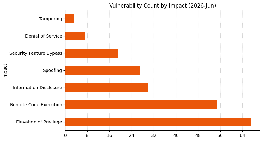
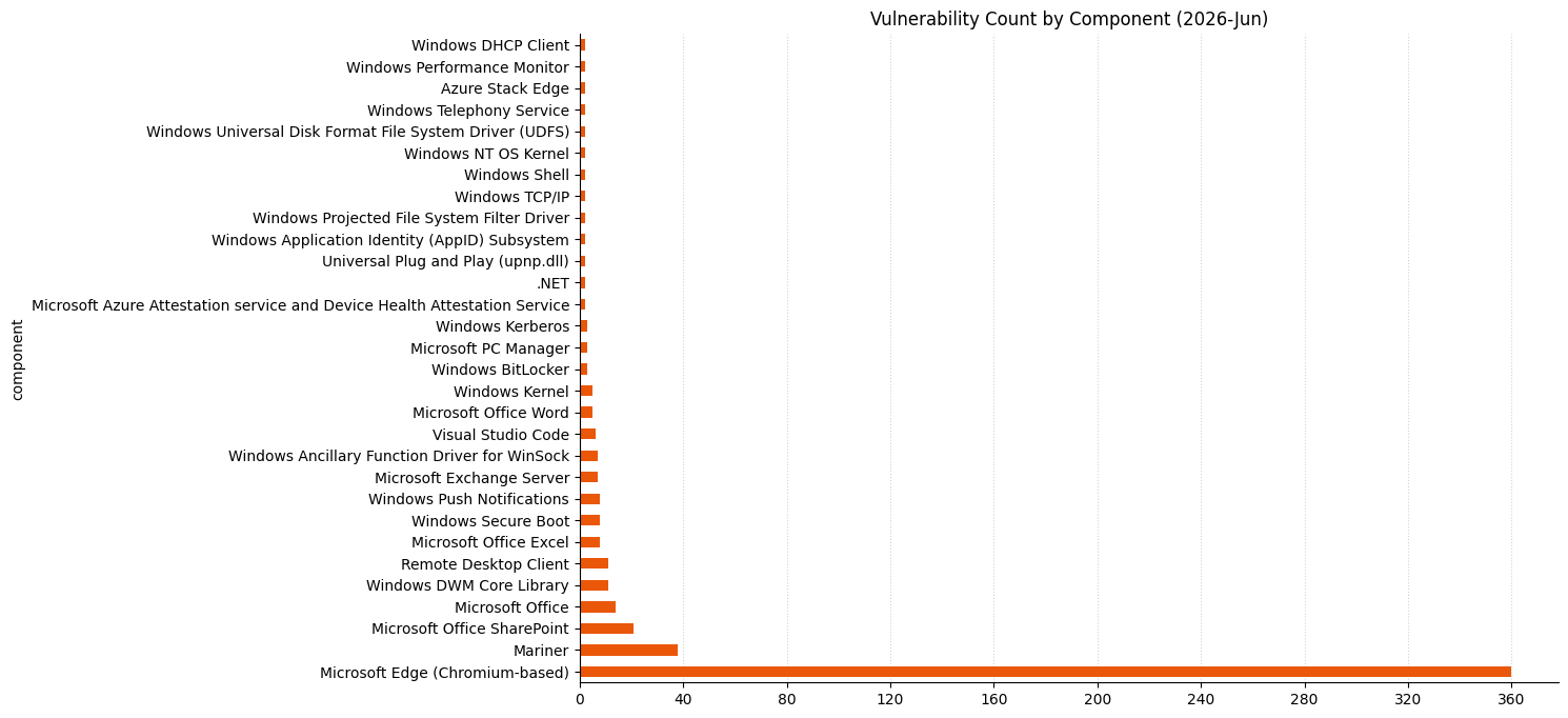
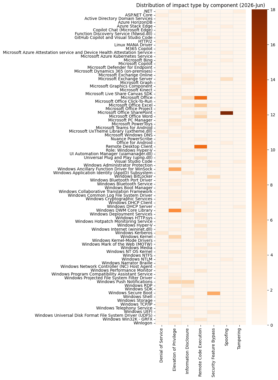
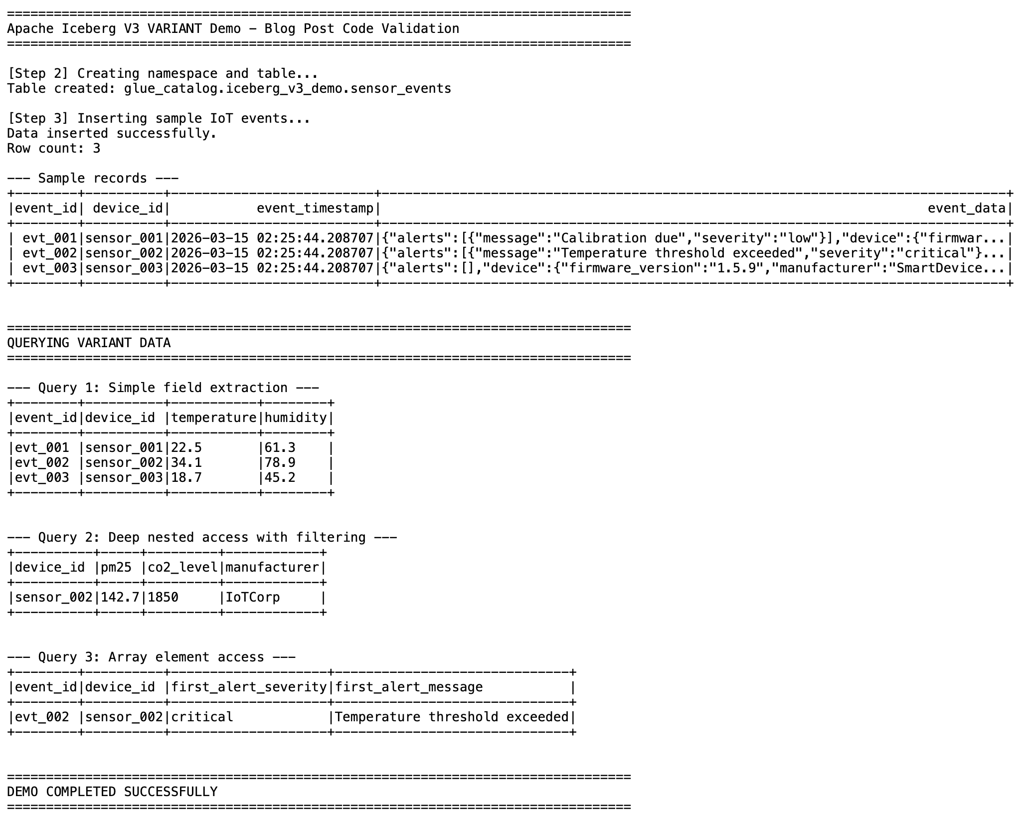

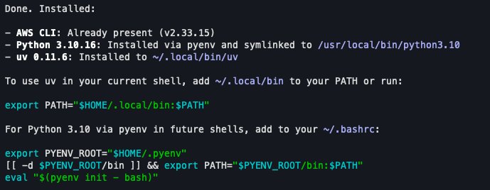
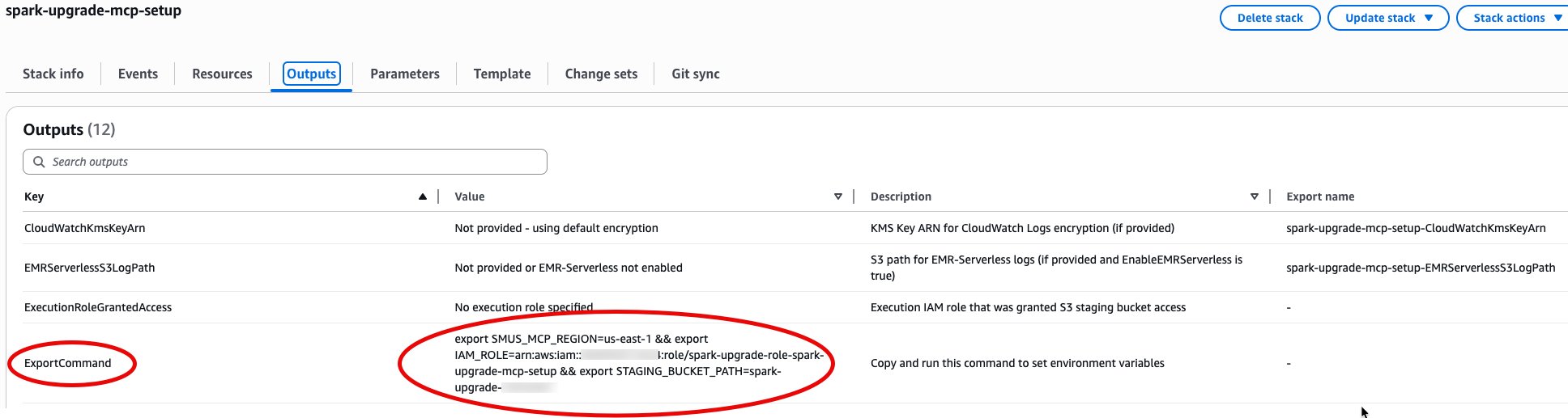
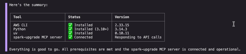
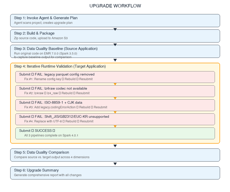
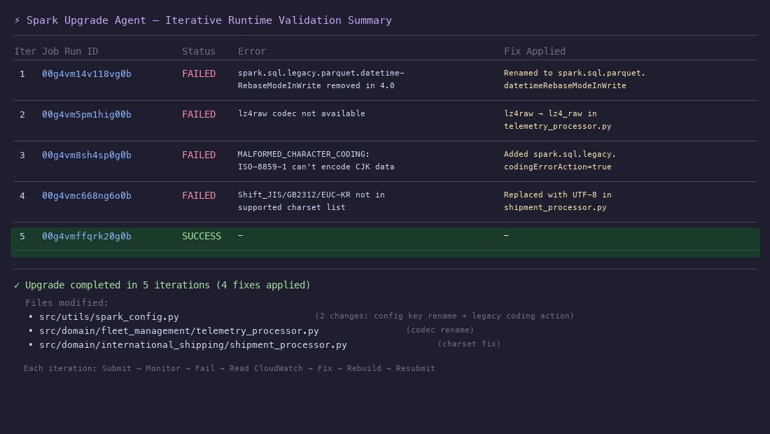
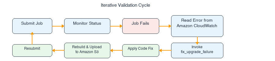
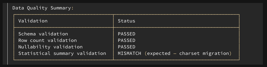
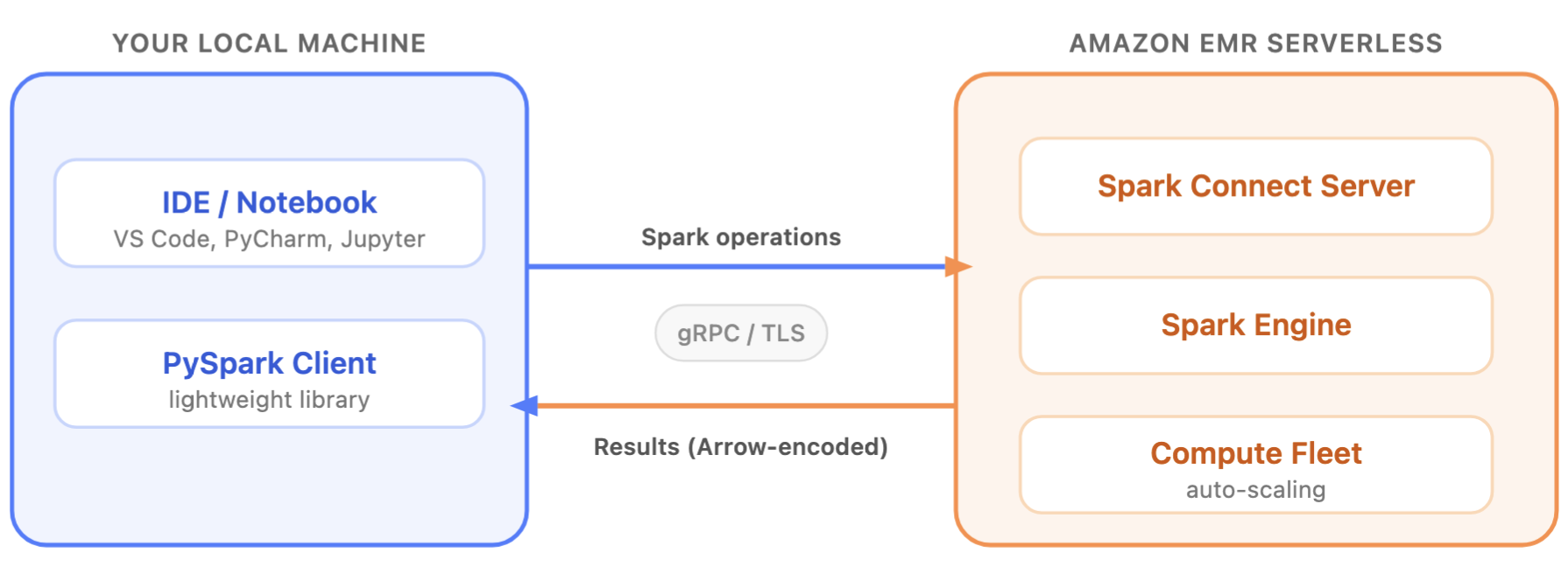
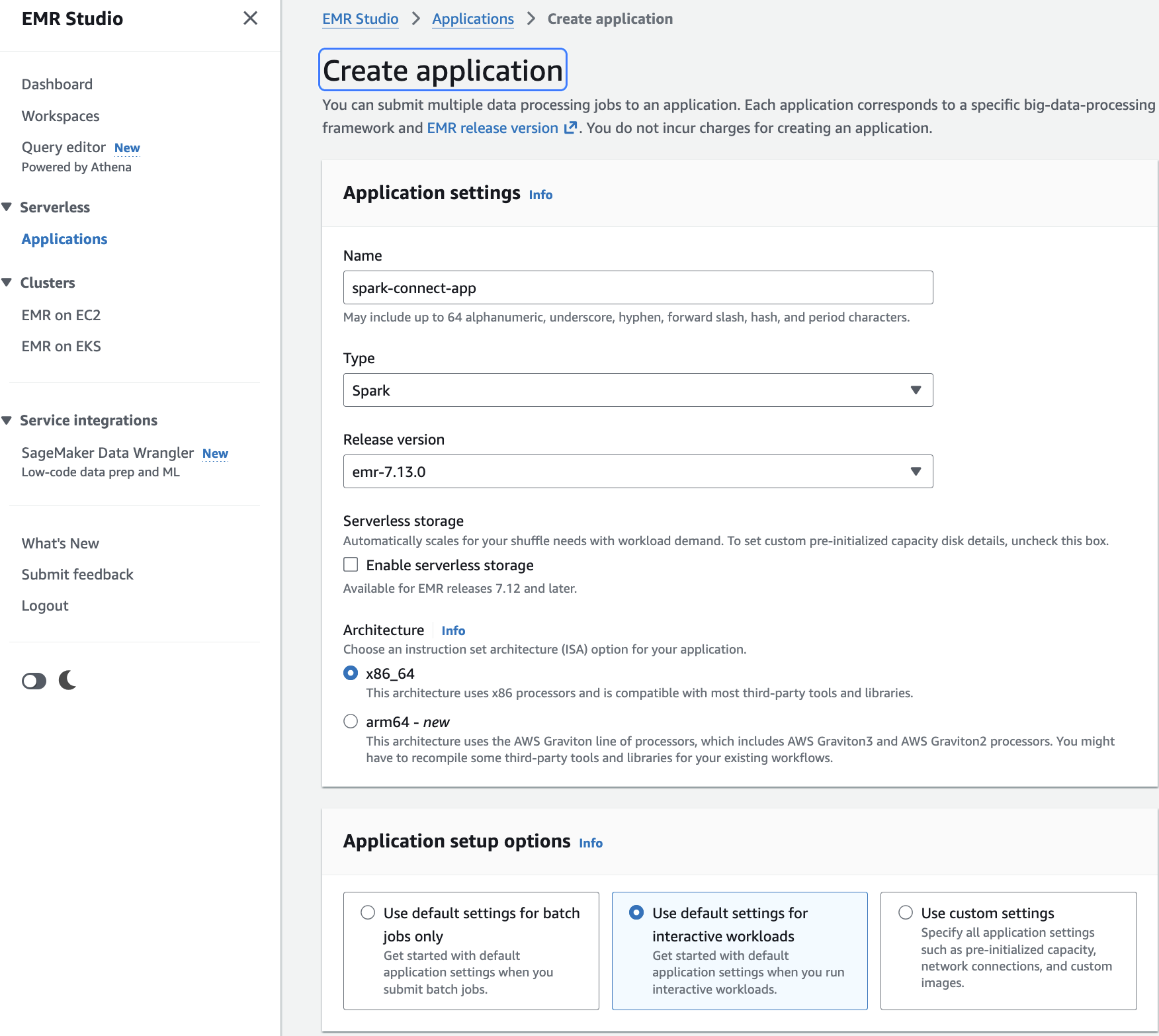
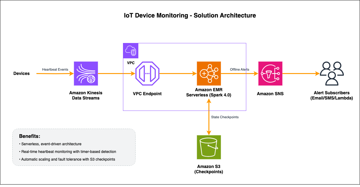
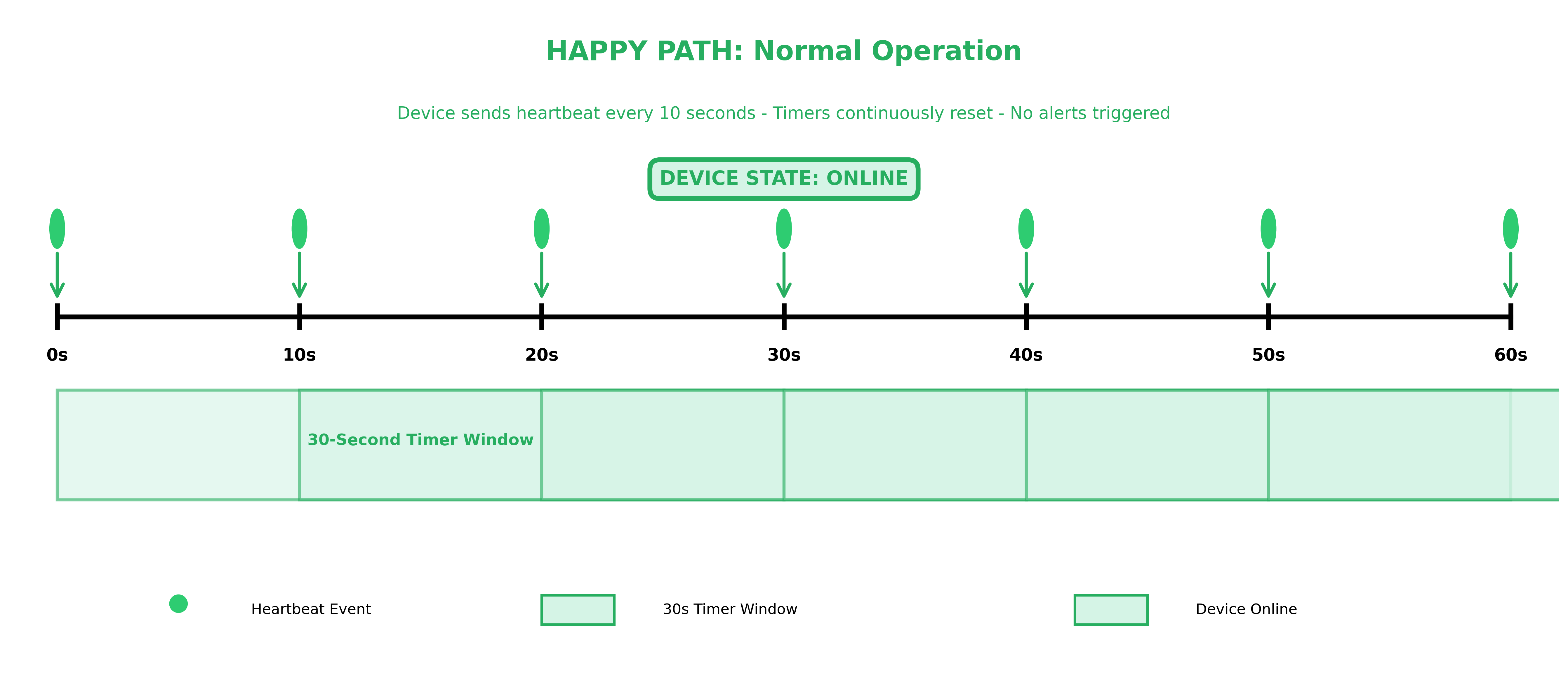
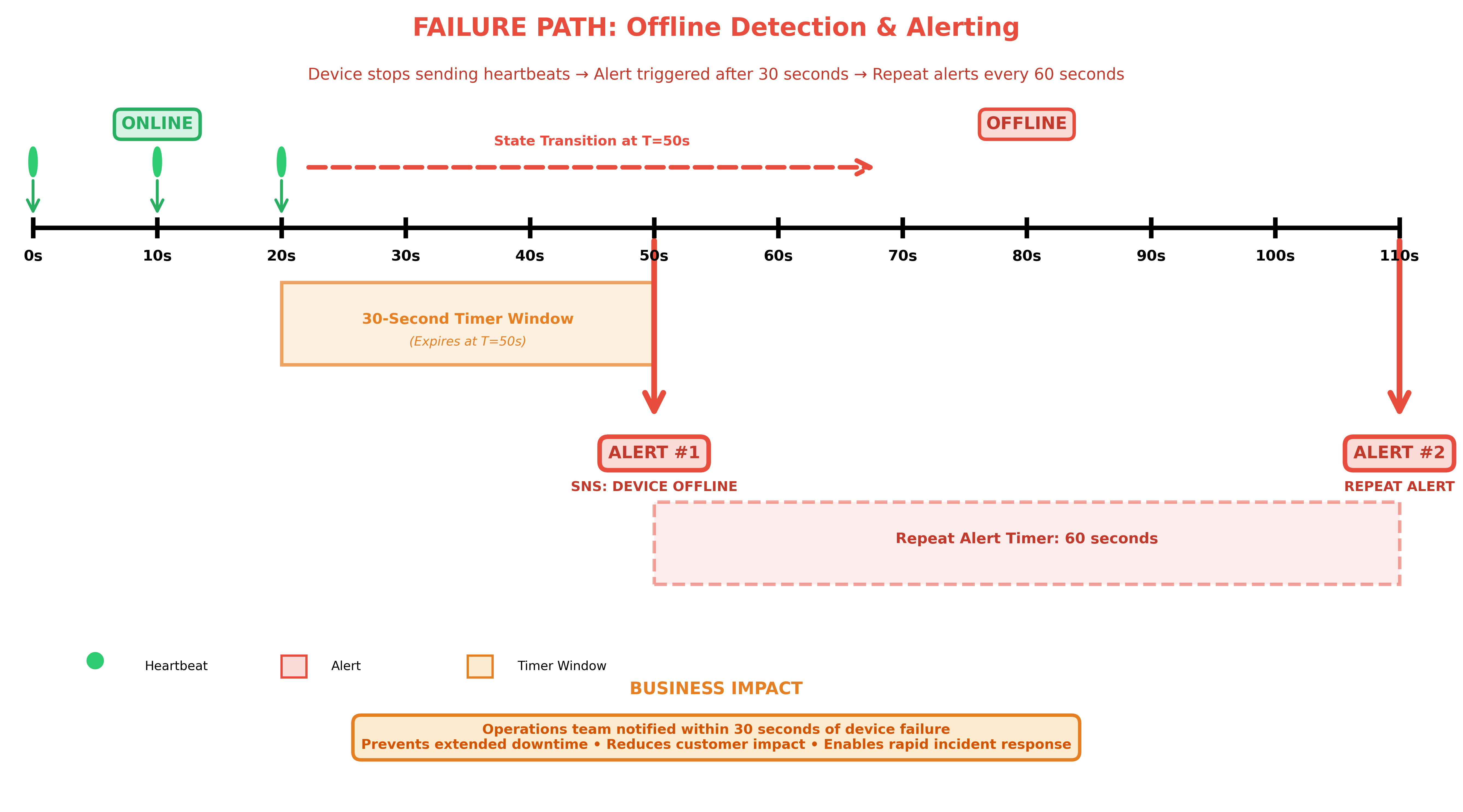
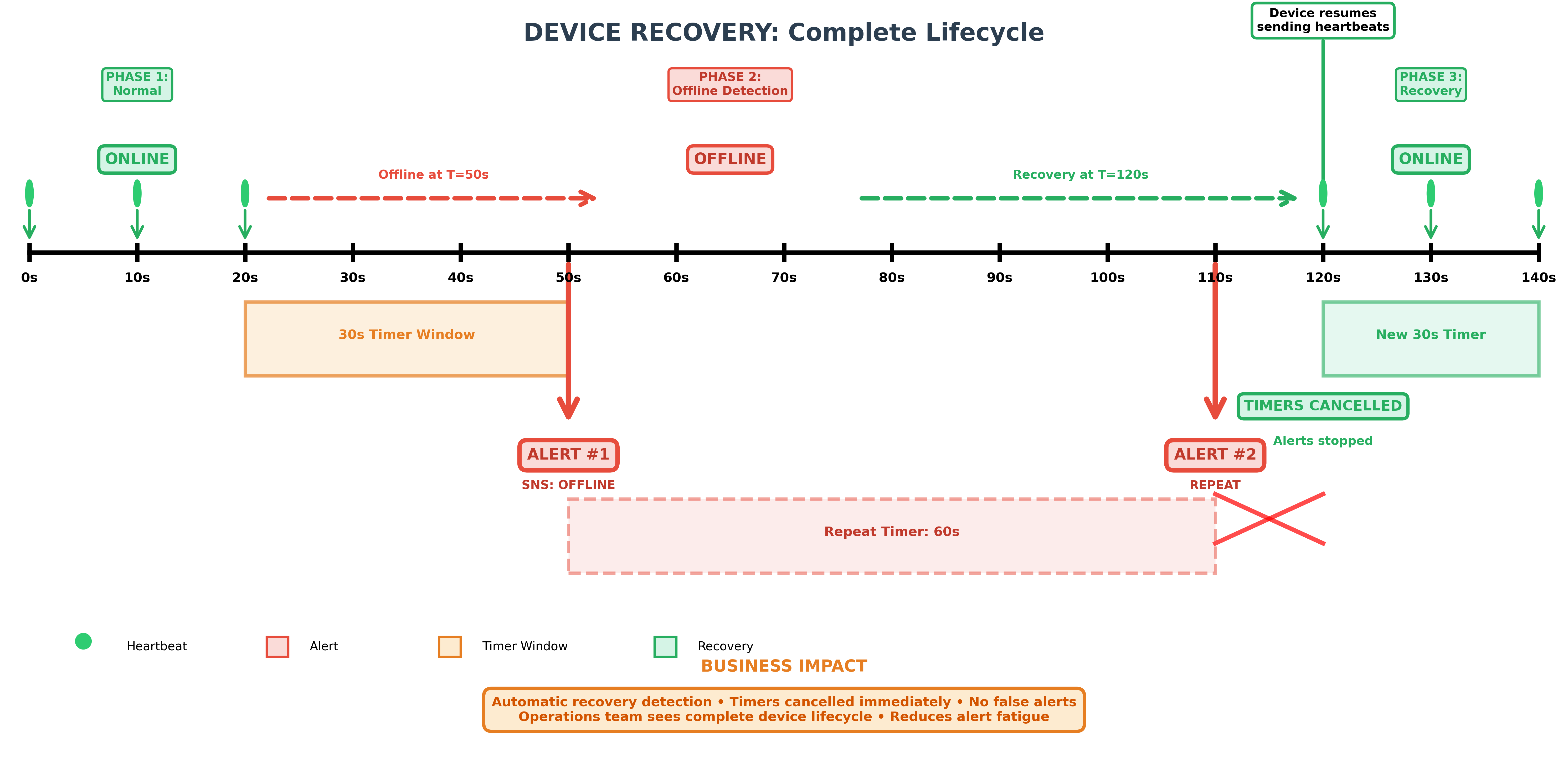
.jpg?ref=toest.bg)