Announcing in-place ZooKeeper-to-KRaft cluster upgrades for Amazon MSK

Post Syndicated from Austin Groeneveld original https://aws.amazon.com/blogs/big-data/announcing-in-place-zookeeper-to-kraft-cluster-upgrades-for-amazon-msk/

Apache Kafka 4.0 officially removes ZooKeeper. If your Amazon Managed Streaming for Apache Kafka (Amazon MSK) Provisioned clusters still run in ZooKeeper metadata mode, now is the time to plan your migration. Amazon MSK now supports in-place upgrades from ZooKeeper to KRaft metadata mode, so you can modernize your existing cluster’s metadata management through the familiar version upgrade workflow.

For more than a decade, Apache ZooKeeper provided dependable metadata management for Kafka, including controller election, partition state, broker registration, and topic configuration. With Apache Kafka 4.0, ZooKeeper is officially removed in favor of KRaft, an embedded Raft-based consensus protocol that handles metadata management internally. It brings those responsibilities into Apache Kafka itself, creating a more streamlined foundation for the continued evolution of Kafka. Amazon MSK has supported KRaft-mode clusters since May 2024, and all Kafka 4.x versions on Amazon MSK use KRaft.

With the in-place upgrade, you can retain your cluster data and metadata while Amazon MSK manages the control-plane transition. Your cluster remains available for produce and consume traffic throughout the process, with no expected downtime if you’re following best practices. By using the existing version upgrade workflow, the move to KRaft becomes a natural step in your cluster’s lifecycle. This prepares your cluster for Kafka 4.x and future Kafka releases.

Prerequisites

Before initiating the upgrade, review the following requirements to confirm your cluster is ready for the transition.

Supported source versions

Clusters must be running Kafka 3.9.x in ZooKeeper mode to use the in-place upgrade. If your cluster is running an earlier version, such as 3.6.0, 3.7.x, or 3.8.x, first complete a standard in-place version upgrade to 3.9.x. You can then initiate the upgrade to 3.9.x.kraft.

Kafka 3.9 is the bridge release for this transition because it supports both ZooKeeper and KRaft modes. To support customers through this migration process, Amazon MSK provides extended support for 3.9.x for a minimum of 2 years from its April 2025 release.

Client compatibility

Requirement Detail
Minimum client library Apache Kafka client v3.0+
Recommended client version v3.9 or above
Connection strings Must use bootstrap.servers only. Any ZooKeeper connection strings (the --zookeeper flag) must be removed before upgrade.

The --zookeeper admin flag was deprecated in Kafka 2.5 and removed in 3.0. Before upgrading, update any remaining applications or tools that connect directly to ZooKeeper.

Pre-upgrade checklist

Before beginning the upgrade, confirm the following:

  • For Standard brokers, the cluster must be deployed across three Availability Zones. Express brokers provide this by default.
  • The cluster is running Kafka 3.9.x in ZooKeeper mode.
  • Standard brokers expose direct ZooKeeper access on ports 2181 (plaintext) and 2182 (TLS). Before upgrading, validate that you’ve disabled ZooKeeper access on the cluster and none of your applications rely on these connections.
  • Solutions using dynamic Kafka configurations that relied on ZooKeeper have been removed before attempting the upgrade operation.
    • If you previously configured custom domain names on a ZooKeeper-based deployment using the dynamic override (kafka-configs.sh --alter on advertised.listeners), be aware that KRaft does not support this dynamic configuration. If you attempt to upgrade your MSK cluster to KRaft with altered advertised.listeners, the upgrade operation fails.
    • If you’re implementing your custom domain name solution on MSK moving forward with KRaft, we recommend our coinciding MSK release for custom domain name support by statically configuring the custom.advertised.listeners property through the UpdateClusterConfiguration API.
  • The cluster has no under-replicated partitions.
  • The cluster is running within per-broker partition limits for standard or express broker clusters.
  • For clusters running above the KRaft brokers-per-cluster limit, you might need an additional quota increase. If you previously raised a quota increase for your ZooKeeper brokers-per-cluster, submit another quota increase for the KRaft limit before attempting the upgrade.
  • The cluster has enough reserve capacity to support rolling broker restarts while serving client traffic.
  • As a best practice, verify that monitoring is ready for the transition from ZooKeeper-specific metrics to KRaft controller metrics.
    • After the migration, ZooKeeper-specific Amazon CloudWatch metrics such as ZookeeperRequestLatencyMsMean and ZookeeperSessionState are no longer available.
    • If you use Open Monitoring, Kafka also stops publishing ZooKeeper metrics. Plan to update or retire related alerts and dashboards as part of your migration preparation.

How the upgrade works

When you initiate the upgrade, Amazon MSK performs a managed, multi-phase migration:

  1. Controller quorum bootstrap: Amazon MSK provisions KRaft controller nodes alongside the existing ZooKeeper infrastructure. Both systems operate in parallel during this phase.
  2. Metadata migration: The KRaft controller reads the cluster state from ZooKeeper and writes it to the internal KRaft metadata log.
  3. Broker transition: Amazon MSK performs a rolling update and registers with the KRaft controller quorum. Data plane operations remain available during the transition.
  4. Validation and bake period: Amazon MSK verifies cluster health under KRaft, including partition leadership, replication state, and controller responsiveness.
  5. ZooKeeper decommissioning: After validation succeeds, Amazon MSK removes the ZooKeeper infrastructure and the cluster operates entirely in KRaft mode.

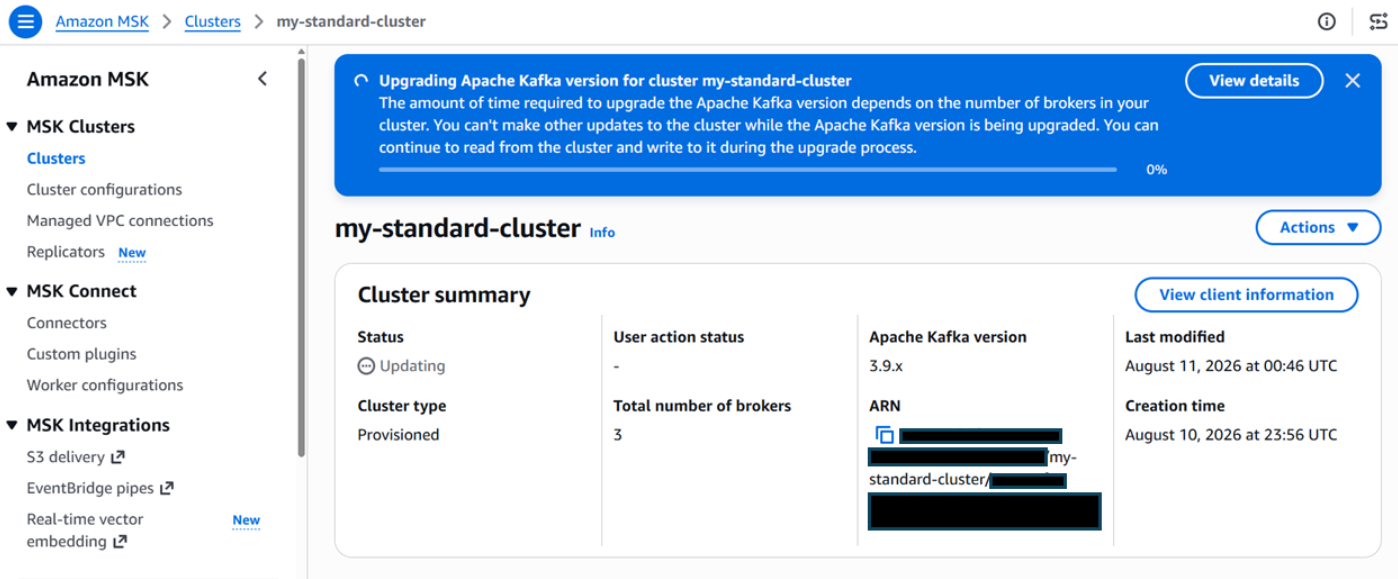
During the upgrade, the cluster enters UPDATING state. You can continue producing and consuming data, while Amazon MSK administrative API operations are temporarily unavailable until the cluster returns to ACTIVE.

Amazon MSK maintains a high bar for durability during the transition. It uses rigorous safety checks at each phase of the migration to protect customer metadata in both roll-forward and rollback scenarios.

Built-in recovery

Amazon MSK monitors cluster health throughout the upgrade. If it detects a condition that prevents the migration from completing, it automatically returns the cluster to its pre-migration state. No customer action is required during recovery.

The operation status changes to Reverting to pre-migration state while Amazon MSK restores the original Kafka version and reconnects ZooKeeper. After the cluster returns to ACTIVE, the describe-cluster-operation API provides error codes, failure reasons, and recommended remediation steps. You can use these to address the issue before starting the upgrade again.

How to perform the upgrade

The following steps walk you through the upgrade process using the Amazon MSK console. You can also perform these steps programmatically using the AWS Command Line Interface (AWS CLI) or SDK.

Step 1: Disable ZooKeeper access (standard brokers only)

Note: This step applies only to Standard broker clusters. Express broker clusters don’t expose direct ZooKeeper access and can skip directly to Step 2.

Standard brokers expose direct ZooKeeper access on ports 2181 (plaintext) and 2182 (TLS). Before upgrading, validate that none of your applications rely on these connections.

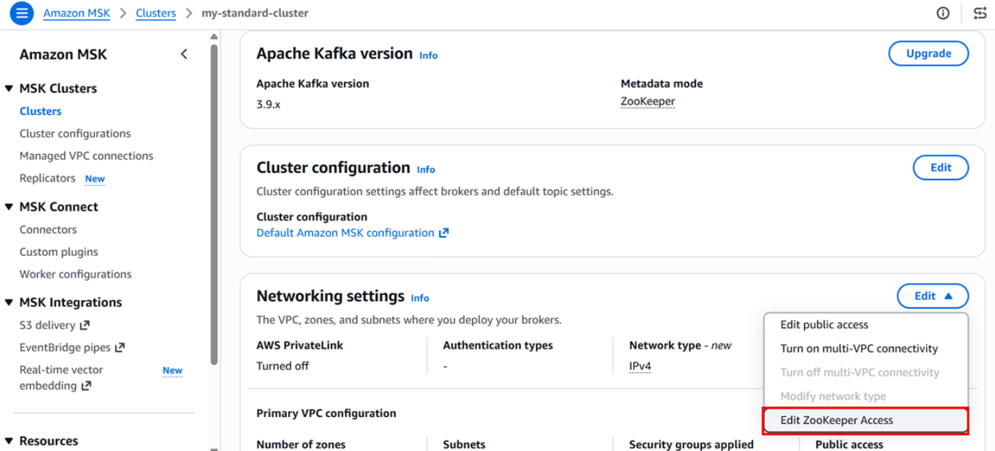
Navigate to your cluster’s Properties tab, choose Network settings, and then choose Edit ZooKeeper access.

Figure 1: Editing ZooKeeper access from the cluster network settings

Figure 1: Editing ZooKeeper access from the cluster network settings

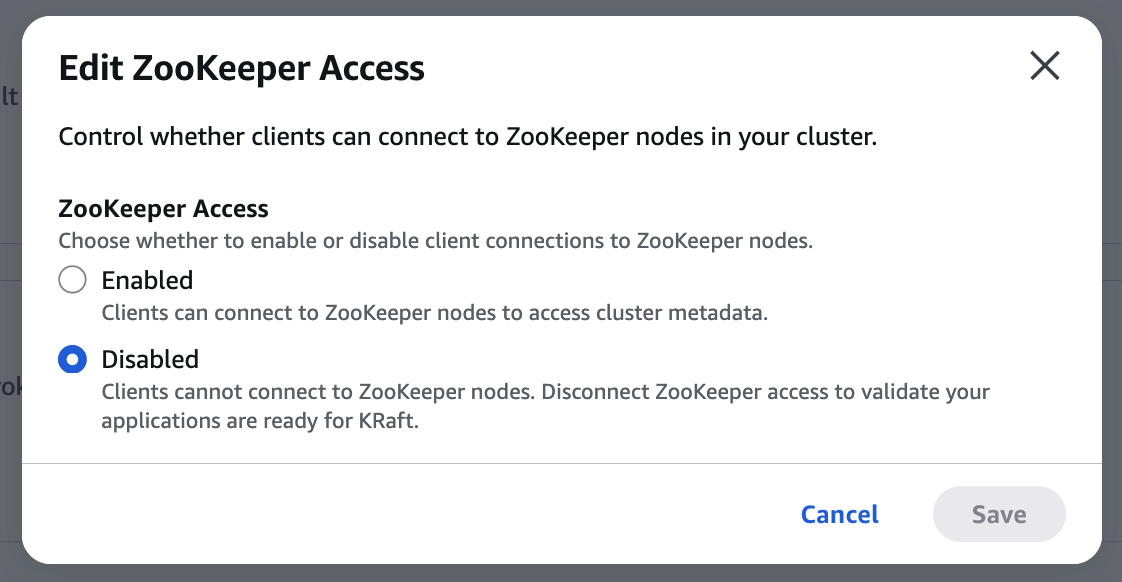
In the pop-up window, verify that ZooKeeper access is set to Disabled, and then choose Save.

Edit ZooKeeper access dialog with access set to Disabled and the Save button

Figure 2: Confirming ZooKeeper access is disabled

Confirm that producers, consumers, and admin tooling continue operating normally without ZooKeeper connectivity. This step is fully reversible. Re-enable ZooKeeper access immediately if anything breaks.

Figure 3: Verifying client traffic continues without ZooKeeper access

Step 2: Initiate the version upgrade

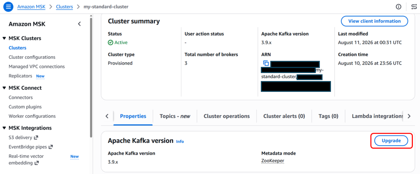
In the Amazon MSK console, under Properties, choose Upgrade in the Apache Kafka version section.

Figure 4: Starting a version upgrade from the Apache Kafka version section

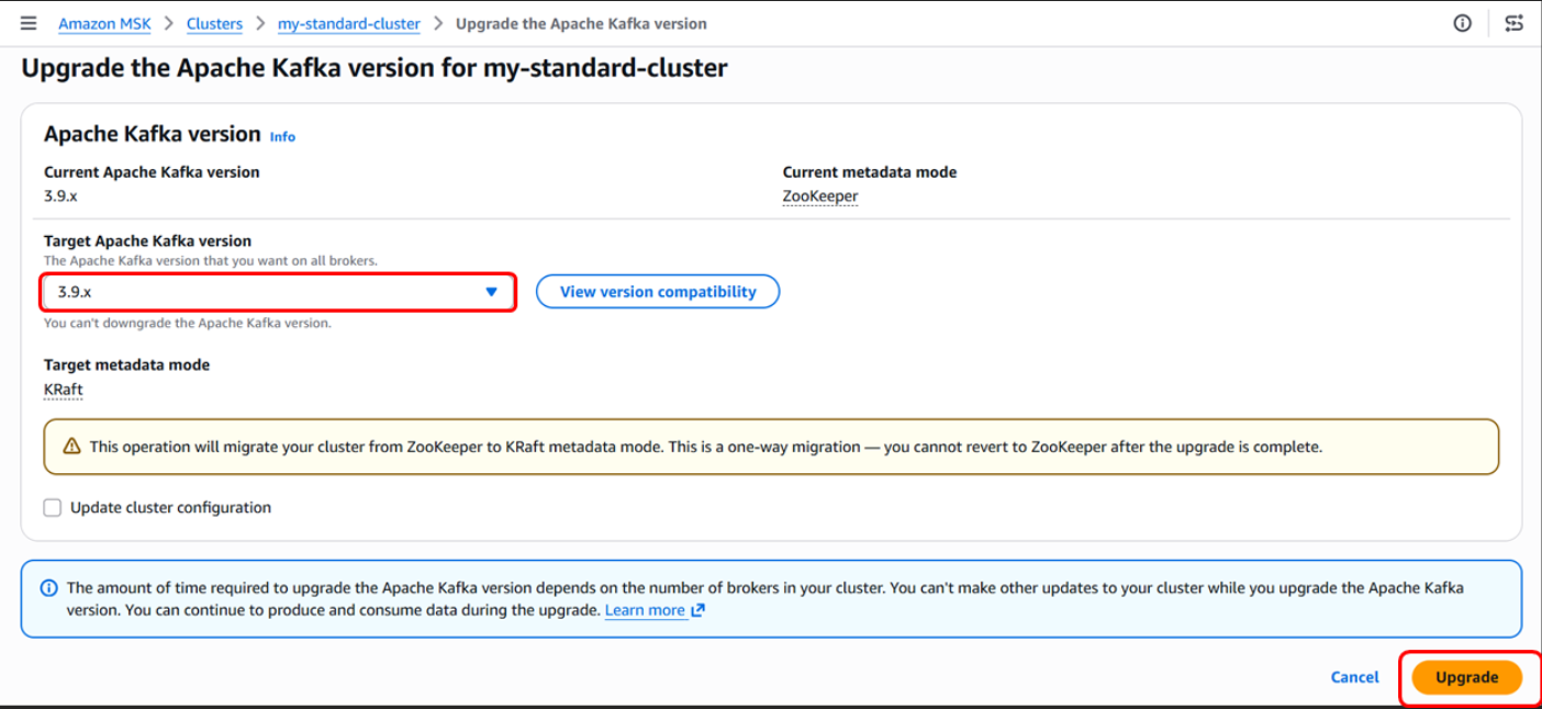
Select your cluster and start a version upgrade to 3.9.x with Target metadata mode set to KRaft. Choose Upgrade.

Figure 5: Selecting KRaft as the target metadata mode

You can monitor your upgrade progress on the cluster properties page.

Figure 6: Monitoring upgrade progress on the cluster properties page

Step 3: Monitor upgrade progress

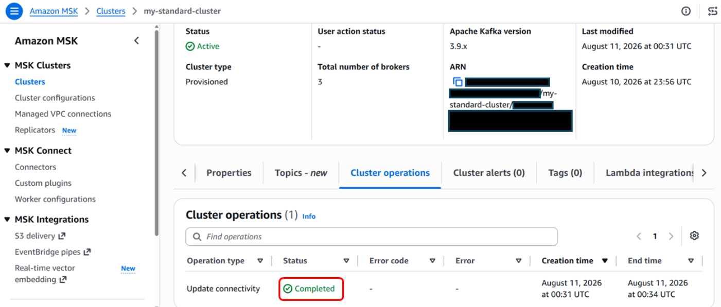
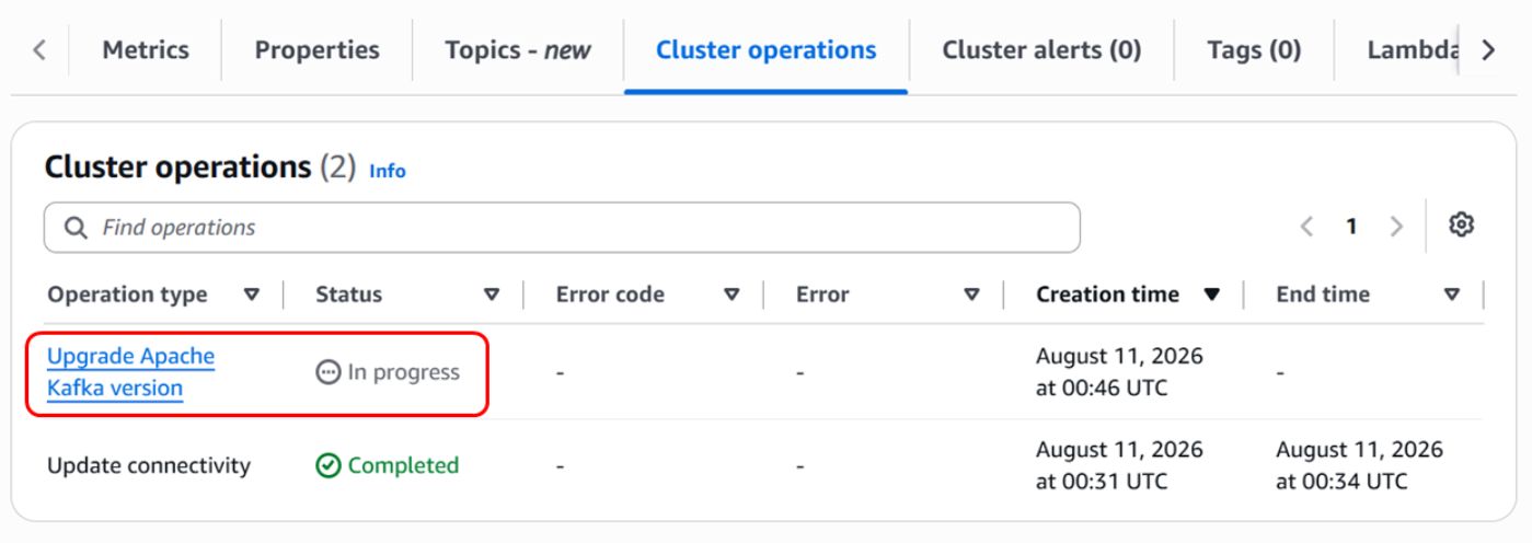
Track progress on the Cluster operations tab in the Amazon MSK console or with the describe-cluster-operation API.

Figure 7: Tracking the upgrade on the Cluster operations tab

Step 4: Validate the KRaft cluster

After the cluster returns to ACTIVE state in KRaft mode:

  • Verify that topics, partitions, and consumer groups are present.
  • Confirm producer and consumer throughput aligns with pre-migration baselines.
  • Update or disable any ZooKeeper-specific monitoring alerts.
  • Update operational documentation and runbooks to reflect KRaft mode.

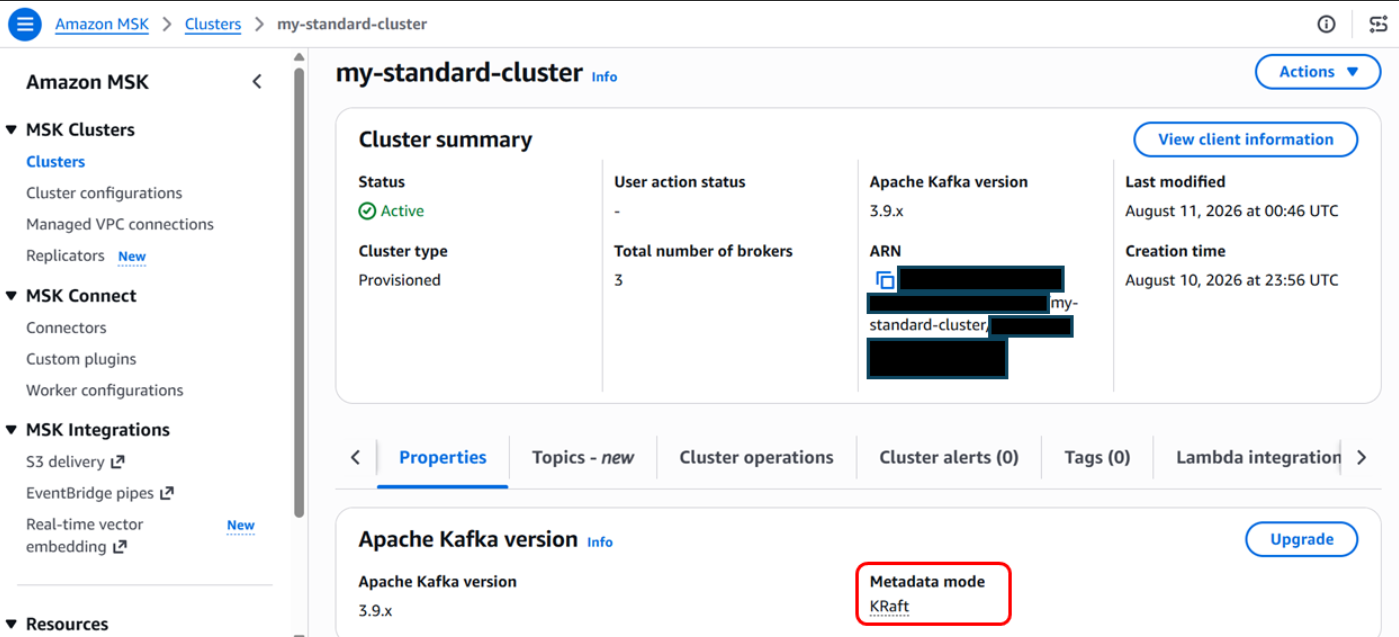
Figure 8: Cluster running in KRaft mode after the upgrade

After the upgrade completes, your cluster appears in an Active state with KRaft enabled as the metadata mode.

Get ready for the next generation of Kafka on Amazon MSK

The in-place ZooKeeper-to-KRaft mode upgrade makes it straightforward to prepare existing Amazon MSK clusters for the future of Apache Kafka. Beyond removing external metadata dependencies, KRaft delivers faster failover times and higher partition limits per cluster. Amazon MSK handles the entire metadata transition, rolling broker updates, validation, and recovery workflow for you. With the new in-place experience, you have a clear, streamlined path to upgrade on your schedule and unlock enhanced scalability and resilience.

For more details, see the Amazon MSK Developer Guide and the supported Kafka versions documentation.


About the authors

Austin Groeneveld

Austin Groeneveld

Austin is a Streaming Specialist Solutions Architect at Amazon Web Services (AWS), based in the San Francisco Bay Area. In this role, Austin is passionate about helping customers accelerate insights from their data using the AWS platform. He is particularly fascinated by the growing role that data streaming plays in driving innovation in the data analytics space. Outside of his work at AWS, Austin enjoys watching and playing soccer, traveling, and spending quality time with his family.

Ashley Millette

Ashley Millette

Ashley is a Specialist Solutions Architect for Streaming and Analytics at AWS. She partners with customers to design and implement real-time data streaming architectures using services like Amazon MSK, helping them build scalable, cost-effective pipelines that turn data in motion into actionable insights. She is passionate about simplifying complex streaming workloads and enabling customers to modernize their data infrastructure with confidence.

Detecting multi-stage attacks on AWS: A guide to cross-service signal correlation

Post Syndicated from Nisha Kashyap original https://aws.amazon.com/blogs/security/detecting-multi-stage-attacks-on-aws-a-guide-to-cross-service-signal-correlation/

A single alert from one security service tells you something happened. Read that signal alongside activity from other services and your own business context, and you will know whether what happened is part of a multi-stage attack.

Consider a short sequence. An identity calls GetCallerIdentity from a source address it hasn’t previously used. Within minutes, that same identity runs a burst of List and Describe calls across several services, and some of them fail with AccessDenied. Soon after, a large volume of data leaves your environment toward a domain that was registered last week. Amazon GuardDuty might already flag pieces of this, such as the reconnaissance from an unfamiliar source, through finding types like Recon:IAMUser/* or Discovery:S3/*. What you gain from correlating the pieces yourself is a single view of the sequence, tied to your own business context, so you can act on the whole rather than triaging findings one at a time.

This post is for security engineers and security operations teams who run Amazon Web Services (AWS) detection services and want to catch patterns specific to their environment. You will see how AWS detection and your business context fit together, and how to build correlations that use that context. The examples run in Amazon CloudWatch Logs Insights so you can try them today, and the closing section describes how to grow them into an automated pipeline. The walkthrough later in this post lists the prerequisites for these queries.

Start with AWS detection services

Begin with the AWS detection services. They cover the threats common across customers, and everything in this post is built on them.

Turn these on and tune them before you build anything custom. Tuning means adjusting sensitivity to reduce false positives for your environment, choosing which data sources each service monitors, and suppressing findings for known-good patterns.

GuardDuty correlates multi-stage attacks for you

Before you build anything by hand, see what GuardDuty already does for you. Amazon GuardDuty Extended Threat Detection correlates signals across multiple data sources including AWS CloudTrail, Amazon S3 data events, runtime monitoring, Amazon Elastic Kubernetes Service (Amazon EKS) audit logs, and more, then raises a single critical severity attack sequence finding when it spots a multi-stage pattern. It recognizes sequences such as credential compromise followed by data exfiltration, maps them to MITRE ATT&CK tactics, and attaches a timeline and remediation guidance. If you have GuardDuty enabled today, then GuardDuty Extended Threat Detection is already enabled by default and needs no queries from you. For details on how GuardDuty charges apply, see Amazon GuardDuty pricing.

The credential compromise sequence in the opening example is the kind of universal pattern GuardDuty Extended Threat Detection is built to catch, so rely on it for those. Attack sequence findings show up in the GuardDuty console next to your other findings, and they route to Security Hub and your response workflows the same way.

GuardDuty handles the threats that look the same in every account. What it doesn’t have is the context that makes a given action suspicious in your account. That’s what you provide.

Add your business context

Business context is what only you know about your environment: which buckets hold sensitive data, which principals have a reason to touch which resources, which role chains your policy permits, and when your production change windows open. GuardDuty Extended Threat Detection learns from patterns common across customers, but it can’t answer these environment-specific questions. Express them as correlations and you add a detection layer tuned to your environment. Each of the following four patterns turns one of these facts into a query.

Run these queries in the AWS Management Console for CloudWatch by choosing Logs, then Logs Insights, using the CloudWatch Logs Insights query language. Most read CloudTrail events from a CloudWatch Logs log group that your trail delivers to. If your trail writes only to Amazon S3, add CloudWatch Logs delivery on the trail, or run equivalent queries in Amazon Athena (a serverless query service for analyzing data in Amazon S3 using SQL).

Note: The queries and code in this post use placeholder values. Replace them with your own before running: your-sensitive-bucket (your S3 bucket name), your-key-id (your AWS KMS key ID), region (your AWS Region, such as us-east-1), account-id (your 12-digit AWS account ID), and aws-cloudtrail-logs-my-trail (your CloudTrail log group name).

A note on multi-account environments. In AWS Organizations, an organization trail delivers every account’s events to one log group, so these queries work as-is but return cross-account results. Filter by recipientAccountId for account-scoped views. Without an organization trail, run queries per account or use Amazon Security Lake as a central query surface.

The attack chain mapped to AWS services

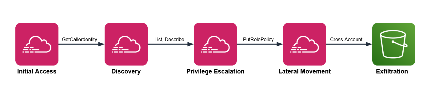
Multi-stage attacks move through five phases, and each phase leaves a signal in a different service. These signals surface across three log sources: CloudTrail, which records API activity in your account; Amazon VPC Flow Logs, which capture network connection metadata; and Amazon Route 53 Resolver query logs, which record DNS queries from your VPCs.

  • Initial access – Stolen credentials reach your environment. CloudTrail records GetCallerIdentity, GetSessionToken, or AssumeRole from an unfamiliar source.
  • Discovery – The threat actor enumerates with List, Describe, and Get calls, often triggering AccessDenied responses.
  • Privilege escalation – The threat actor chains roles or edits policies. CloudTrail records AssumeRole sequences, PutRolePolicy, or CreateAccessKey.
  • Lateral movement – The threat actor moves across accounts or AWS Regions, assuming roles and creating resources in unfamiliar places.
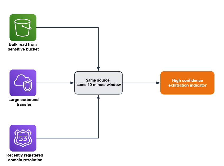
  • Exfiltration – Data leaves through GetObject calls at scale, large outbound transfers in VPC Flow Logs, and DNS queries in Route 53 Resolver query logs to recently registered domains.

Figure 1 shows the five attack phases mapped to the AWS log source that records each one.

Figure 1: Attack chain mapped to AWS services

Figure 1: Attack chain mapped to AWS services

GuardDuty Extended Threat Detection watches this chain for universal patterns. The four patterns that follow add the dimension you supply: your business context.

Pattern one: Sensitive data access by an unexpected principal

Your data classification and access norms drive this detection. One bucket holds customer records, another holds public web assets, and you know which principals have a reason to read the customer records, which are sensitive. Encode that knowledge and an ordinary looking read turns into something worth chasing.

Three signals converge here. CloudTrail shows GetObject at volume on a bucket you’ve classified as sensitive. The principal isn’t on your list of expected readers for that bucket. And VPC Flow Logs show a large outbound transfer from the same source in the same window, while DNS query logs show a recently registered destination domain, which together increase your confidence that there’s a potential threat.

CloudTrail management events don’t record GetObject. You must turn on CloudTrail data events for the buckets you care about to capture GetObject. Many teams miss GetObject because data events weren’t enabled on the relevant buckets.

This query shows bulk reads on a sensitive bucket, grouped by principal. Run it in CloudWatch Logs Insights with your CloudTrail log group selected.

fields @timestamp, userIdentity.arn, requestParameters.bucketName
| filter eventSource = "s3.amazonaws.com" and eventName = "GetObject"
| filter requestParameters.bucketName = "your-sensitive-bucket"
| stats count(*) as objectReads,
        count_distinct(requestParameters.key) as distinctObjects
        by userIdentity.arn, bin(10m)
| filter objectReads > 100
| sort objectReads desc

The threshold of 100 is a placeholder. Run the query over a week of normal activity, find the ninety-fifth percentile read count for that bucket, and set the threshold above it. Then check each principal the query returns against your expected reader list. A principal that isn’t on the list, reading at volume, is the result to investigate.

To corroborate, look for a matching outbound transfer. Switch the log group selector to your VPC Flow Logs log group and run this.

fields @timestamp, srcAddr, dstAddr, bytes
| filter action = "ACCEPT"
# exclude RFC 1918 private ranges so only external destinations remain
| filter dstAddr not like /^10\./
        and dstAddr not like /^192\.168\./
        and dstAddr not like /^172\.(1[6-9]|2[0-9]|3[0-1])\./
| stats sum(bytes) as totalBytes by srcAddr, dstAddr, bin(10m)
| filter totalBytes > 1000000000
| sort totalBytes desc

The Amazon S3 query returns a principal, and the Flow Logs query works on IP addresses, so you translate one into the other. The worked example later in this post covers that translation in full.

Picture an analytics role that reads a reporting bucket all day. One afternoon, it reads a thousand objects from your customer records bucket instead. GuardDuty stays quiet, because an authenticated role making valid GetObject calls isn’t suspicious anywhere else. Your query flags it, because that role isn’t on the expected reader list for that bucket. The classification you applied is what turns silence into a signal.

Figure 2 shows a bulk read from a sensitive bucket in CloudTrail, a large outbound transfer in VPC Flow Logs, and a young domain resolution in Route 53 Resolver logs.

Figure 2: Three signals converging within a single time window to indicate exfiltration

Figure 2: Three signals converging within a single time window to indicate exfiltration

Pattern two: A role chain that crosses your access policy

Picture a deployment that assumes one role to build, then a second to release. For one principal, that two-hop AssumeRole chain is routine; for a different principal it’s a policy violation. This pattern relies on your trust topology—the chains your organization permits—so put that knowledge in the query.

This pattern needs three conditions:

  • CloudTrail shows several AssumeRole calls from the same source inside a short window
  • The chain ends in a sensitive action such as CreateAccessKey, PutRolePolicy, or AttachUserPolicy
  • The starting identity isn’t one your policy expects to run that chain

In CloudWatch Logs Insights, select your CloudTrail log group and run this query, which surfaces chains of two or more hops.

fields @timestamp, userIdentity.arn, requestParameters.roleArn, sourceIPAddress
| filter eventName = "AssumeRole"
| stats count(*) as assumeCount,
        count_distinct(requestParameters.roleArn) as rolesAssumed
        by sourceIPAddress, bin(5m)
| filter assumeCount >= 2 and rolesAssumed >= 2
| sort assumeCount desc

Two hops is the minimum for a chain; raise the count if your environment chains roles often. Your deployment pipeline probably assumes several roles an hour, as do AWS service principals such as AWS Security Hub. Exclude the identities you expect to see assuming multiple roles, including your pipeline role and known AWS service principals. What’s left is the set to investigate, such as a person assuming several roles at an odd hour and ending in a new access key. Treat that distinction as data: list the identities and actions you consider normal, and review the chains that fall outside the list.

Pattern three: An encryption key used outside its owning workload

Resource ownership is the signal here. A given AWS Key Management Service (AWS KMS) key creates and controls the encryption keys for a workload, and a single key should serve a single workload, such as a payments service. A Decrypt call against it is a valid, authorized API action, so nothing about the call itself looks wrong. The ownership rule you set is what makes another principal’s use of the key worth a second look.

This pattern applies only to customer-managed keys scoped to one workload. It doesn’t apply to AWS-managed keys (alias/aws/*) or to customer-managed keys intentionally shared across services. Confirm single-workload intent from the key policy’s Principal block before deploying this rule.

Two conditions indicate misuse:

  • CloudTrail shows Decrypt or GenerateDataKey calls on a key that’s tied to one workload
  • The calling principal isn’t the role that owns that workload

Against your CloudTrail log group, run this query to list the principals that called a specific key.

fields @timestamp, userIdentity.arn, eventName
| filter eventSource = "kms.amazonaws.com"
| filter eventName in ["Decrypt", "GenerateDataKey", "Encrypt"]
| filter resources.0.ARN = "arn:aws:kms:region:account-id:key/your-key-id"
| stats count(*) as keyUses by userIdentity.arn, eventName
| sort keyUses desc

Compare what comes back against the one workload role you expect. A principal you don’t recognize on that key is the signal. Because key misuse is an early move in data theft, this correlation catches activity that only your ownership knowledge can flag.

Consider a key that wraps your payments database. The payments service role calls it in normal operation, and nothing else should. If a developer role or a freshly created role runs Decrypt against it, the call succeeds and reads as ordinary in isolation. The reason it matters is the ownership rule you hold in your head and now state in this query.

Pattern four: A privileged action outside your change window

Start with the query, then read what it means.

fields @timestamp, userIdentity.arn, eventName, sourceIPAddress
| filter eventName in ["PutRolePolicy", "AttachRolePolicy",
        "CreateAccessKey", "AuthorizeSecurityGroupIngress", "PutBucketPolicy"]
| stats count(*) as sensitiveChanges by userIdentity.arn, eventName, sourceIPAddress
| sort sensitiveChanges desc

Run it against your CloudTrail log group, scoped to your off-hours window when you schedule it, so it returns only activity outside the change window. Your change process defines what normal looks like here: production security and identity changes flow through a pipeline during defined hours, run by a known actor. A console-driven policy change at 2:00 AM, made by a person rather than the pipeline, doesn’t fit those expectations. The signal is a sensitive change such as PutRolePolicy or AuthorizeSecurityGroupIngress, made outside the window, by a person rather than your pipeline role.

Exclude the actors you expect, such as your deployment pipeline role, your patch automation role, and AWS service principals like AWS CloudFormation and AWS Systems Manager. What remains is privileged change made outside your process, which is both what an attacker does to establish persistence and what your own change discipline says shouldn’t happen.

Your pipeline might open security group rules during a deployment every weekday afternoon. A person opening a security group rule at midnight on a weekend is the same API call carrying a very different meaning. The schedule and the actor, both facts you define, are what separate the two.

Build your first correlation rule

The following walkthrough uses pattern one as a complete example. The other three patterns follow the same design with their own queries.

Prerequisites

These prerequisites feed the queries in this walkthrough. Confirm each one before you start:

  • A CloudTrail trail logging management events to a CloudWatch Logs log group
  • CloudTrail data events enabled for your sensitive S3 buckets
  • GuardDuty enabled, with its protection plans and Extended Threat Detection
  • VPC Flow Logs on for your production VPCs
  • Amazon Route 53 Resolver query logging on

CloudTrail, GuardDuty, VPC Flow Logs, and Route 53 Resolver query logging provide the raw signals that your correlations connect. Without them, the queries in this post return empty results.

Step 1: Record the bucket and its expected readers

Choose one sensitive bucket to monitor, and write down the principals allowed to read it. Store the list where your automation can reach it, such as a configuration file in version control or an Amazon DynamoDB table (a managed NoSQL database).

{
  "customer-records-prod": [
    "arn:aws:iam::123456789012:role/AnalyticsPipeline",
    "arn:aws:iam::123456789012:role/ComplianceAudit"
  ],
  "financial-data-archive": [
    "arn:aws:iam::123456789012:role/FinanceReporting"
  ]
}

This example hardcodes the list for simplicity. In production, load it from a DynamoDB table or Parameter Store so you can update it without redeploying.

Step 2: Baseline before you set a threshold

Run the pattern one query over one week of normal activity. Find the 95th percentile read count for the bucket and use a value greater than that as your alert threshold. This step keeps legitimate high-volume access from generating false positives later.

Set the THRESHOLD_READS environment variable to this value when you configure the function in Step 5.

Step 3: Run the access query

In the CloudWatch console:

  1. Choose Logs, then choose Logs Insights.
  2. In the Select log group(s) dropdown, select your CloudTrail log group.
  3. Set the time range to 3h (the last three hours).
  4. In the query editor, paste the pattern one query.
  5. Replace your-sensitive-bucket with your bucket name.
  6. Choose Run query.
  7. Review the principals in the results table.
  8. Compare each principal against your expected reader list from step 1, and flag any that are not on it.

Each result includes a principal that step 4 translates into an IP address.

Step 4: Correlate with network activity

CloudTrail logs actions by AWS Identity and Access Management (IAM) principal, while VPC Flow Logs record traffic by IP address. To connect the two signals, translate the principal into its address.

For a role attached to an Amazon Elastic Compute Cloud (Amazon EC2) instance, the userIdentity.principalId field includes the instance ID after the colon, in the form AROAEXAMPLE:i-1234567890abcdef0. Copy the instance ID and look up its private IP address.

aws ec2 describe-instances \
  --instance-ids i-1234567890abcdef0 \
  --query "Reservations[0].Instances[0].PrivateIpAddress" \
  --output text

Other compute types differ. A VPC-connected AWS Lambda function sends traffic through elastic network interfaces in your subnets, so correlate on those interface addresses. An Amazon Elastic Container Service (Amazon ECS) task records its network interface in task metadata. For a plain assumed-role session with no instance behind it, the sourceIPAddress field in CloudTrail already holds the caller’s address, so you correlate on it directly.

Run the Flow Logs query from pattern one, filtering srcAddr to that address within 10 minutes of the Amazon S3 read timestamp. A match places the same source behind both the sensitive read and a large external transfer in one window. CloudTrail events reach CloudWatch Logs 5–15 minutes after the API call, so correlate on eventTime rather than query time. Query a wider lookback than your correlation window: for example, look back 30 to 60 minutes but correlate on a 10-minute eventTime window. Steps 3 and 4 are manual validation; step 5 automates them.

Figure 2 shows DNS resolution as a third corroborating signal. This walkthrough implements the CloudTrail and VPC Flow Logs correlation. To add DNS, apply the same run_query() pattern against your Route 53 Resolver query log group.

Step 5: Automate the check

Move the query into a Lambda function (serverless compute that runs your code without a server to manage), send results to a notification channel, and schedule regular runs. Work through the following sub-procedures.

To create the notification channel

  1. Open the Amazon Simple Notification Service (Amazon SNS) console. Amazon SNS is a managed messaging service that delivers notifications to subscribers.
  2. In the navigation pane, choose Topics.
  3. Choose Create topic.
  4. For Type, select Standard.
  5. For Name, enter security-correlation-alerts.
  6. Choose Create topic.
  7. Note the topic Amazon Resource Name (ARN) at the top of the topic details page. You will use it in the function.
  8. Choose Create subscription.
  9. For Protocol, select Email.
  10. For Endpoint, enter your email address or incident management endpoint.
  11. Choose Create subscription, then confirm the subscription from the email AWS sends.

To create the EventBridge Scheduler execution role

The schedule needs a role that lets it invoke your function, and its trust policy needs conditions that pin the role to the schedule you own. Without those conditions, another account with access to the scheduler service could theoretically call this role; a class of misuse known as the confused deputy problem.

1. Create a trust policy file named scheduler-trust-policy.json.

{
  "Version": "2012-10-17",
  "Statement": [
    {
      "Effect": "Allow",
      "Principal": { "Service": "scheduler.amazonaws.com" },
      "Action": "sts:AssumeRole",
      "Condition": {
        "StringEquals": {
          "aws:SourceAccount": "ACCOUNT-ID"
        },
        "ArnLike": {
          "aws:SourceArn": "arn:aws:scheduler:REGION:ACCOUNT-ID:schedule/*/s3-access-correlation-hourly"
        }
      }
    }
  ]
}

2. Create the role, then attach permission to invoke the function. Scope Resource to the specific function ARN so this role can’t invoke anything else.

aws iam create-role \
  --role-name EventBridgeSchedulerRole \
  --assume-role-policy-document file://scheduler-trust-policy.json

aws iam put-role-policy \
  --role-name EventBridgeSchedulerRole \
  --policy-name LambdaInvokePolicy \
  --policy-document '{
    "Version": "2012-10-17",
    "Statement": [
      {
        "Effect": "Allow",
        "Action": "lambda:InvokeFunction",
        "Resource": "arn:aws:lambda:REGION:ACCOUNT-ID:function:CorrelationFunction"
      }
    ]
  }'

When you create the function, Lambda automatically creates an execution role. You will attach the permissions this function needs to that role in a later step.

To deploy the correlation function

  1. Open the Lambda console.
  2. Choose Create function.
  3. For Function name, enter CorrelationFunction.
  4. For Runtime, select the latest Python runtime.
  5. Choose Create function.
  6. On the Code tab, replace the default code with the following function, then choose Deploy.
import os
import time
import logging
import boto3
from botocore.exceptions import ClientError

logger = logging.getLogger()
logger.setLevel(logging.INFO)

logs = boto3.client("logs")
sns = boto3.client("sns")
ec2 = boto3.client("ec2")

CLOUDTRAIL_LOG_GROUP = os.environ["CLOUDTRAIL_LOG_GROUP"]
FLOWLOGS_LOG_GROUP = os.environ["FLOWLOGS_LOG_GROUP"]
SNS_TOPIC = os.environ["SNS_TOPIC_ARN"]
BUCKET = os.environ["SENSITIVE_BUCKET"]
THRESHOLD = int(os.environ.get("THRESHOLD_READS", "100"))

# Expected readers per bucket
EXPECTED_READERS = {
    "customer-records-prod": [
        "arn:aws:iam::123456789012:role/AnalyticsPipeline",
        "arn:aws:iam::123456789012:role/ComplianceAudit",
    ],
}


def run_query(log_group, query, start, end):
    """Start a Logs Insights query and wait for it to finish."""
    started = logs.start_query(
        logGroupName=log_group,
        startTime=start,
        endTime=end,
        queryString=query,
    )
    query_id = started["queryId"]
    while True:
        outcome = logs.get_query_results(queryId=query_id)
        if outcome["status"] in ("Complete", "Failed", "Cancelled"):
            break
        time.sleep(1)
    if outcome["status"] != "Complete":
        raise RuntimeError(f"Query did not complete: {outcome['status']}")
    return [{f["field"]: f["value"] for f in row} for row in outcome["results"]]


def private_ip_for_principal(principal_id):
    """Resolve an EC2 instance role principalId to its private IP."""
    if ":" not in principal_id:
        return None
    instance_id = principal_id.split(":", 1)[1]
    if not instance_id.startswith("i-"):
        return None
    reservations = ec2.describe_instances(InstanceIds=[instance_id])
    for reservation in reservations["Reservations"]:
        for instance in reservation["Instances"]:
            return instance.get("PrivateIpAddress")
    return None


def egress_bytes(src_addr, start, end):
    """Sum external egress bytes for one source address."""
    query = f"""
    fields srcAddr, dstAddr, bytes
    | filter action = "ACCEPT" and srcAddr = "{src_addr}"
    | filter dstAddr not like /^10\\./
            and dstAddr not like /^192\\.168\\./
            and dstAddr not like /^172\\.(1[6-9]|2[0-9]|3[0-1])\\./
    | stats sum(bytes) as totalBytes
    """
    rows = run_query(FLOWLOGS_LOG_GROUP, query, start, end)
    if rows and rows[0].get("totalBytes"):
        return int(rows[0]["totalBytes"])
    return 0


def lambda_handler(event, context):
    try:
        # 1-hour lookback absorbs CloudTrail's 5-15 min delivery latency;
        # correlation happens on eventTime via 10-min bins in the query below.
        end = int(time.time())
        start = end - 3600  # 1 hour lookback
        allowed = EXPECTED_READERS.get(BUCKET, [])

        access_query = f"""
        fields userIdentity.arn, userIdentity.principalId
        | filter eventSource = "s3.amazonaws.com" and eventName = "GetObject"
        | filter requestParameters.bucketName = "{BUCKET}"
        | stats count(*) as objectReads
                by userIdentity.arn, userIdentity.principalId, bin(10m)
        | filter objectReads > {THRESHOLD}
        """

        for row in run_query(CLOUDTRAIL_LOG_GROUP, access_query, start, end):
            principal = row.get("userIdentity.arn")
            if not principal or principal in allowed:
                continue

            message = (
                f"Principal {principal} read {row.get('objectReads')} "
                f"objects from {BUCKET}."
            )

            ip = private_ip_for_principal(row.get("userIdentity.principalId", ""))
            if ip and egress_bytes(ip, start, end) > 1_000_000_000:
                message += (
                    f" The same source ({ip}) also sent a large volume of "
                    f"data to external destinations in the same window."
                )

            sns.publish(
                TopicArn=SNS_TOPIC,
                Subject="Unexpected S3 access detected",
                Message=message,
            )
    except ClientError as error:
        logger.error(f"AWS API error: {error}")
        raise
    except Exception as error:
        logger.error(f"Unexpected error: {error}")
        raise
    finally:
        logger.info("Correlation check completed")

  1. On the Configuration tab, choose General configuration, then choose Edit. Set Timeout to 5 minutes (300 seconds). CloudWatch Logs Insights queries run asynchronously and can take 30 to 60 seconds against large log groups. Choose Save.
  2. On the Configuration tab, choose Environment variables, then choose Edit, and add CLOUDTRAIL_LOG_GROUP, FLOWLOGS_LOG_GROUP, SNS_TOPIC_ARN, SENSITIVE_BUCKET, and THRESHOLD_READS.
  3. On the Configuration tab, choose Permissions, open the execution role, and attach the following least-privilege policy.
{
  "Version": "2012-10-17",
  "Statement": [
    {
      "Effect": "Allow",
      "Action": ["logs:StartQuery", "logs:GetQueryResults"],
      "Resource": [
        "arn:aws:logs:REGION:ACCOUNT-ID:log-group:aws-cloudtrail-logs-my-trail:*",
        "arn:aws:logs:REGION:ACCOUNT-ID:log-group:vpc-flow-logs:*"
      ]
    },
    {
      "Effect": "Allow",
      "Action": "ec2:DescribeInstances",
      "Resource": "*"
    },
    {
      "Effect": "Allow",
      "Action": "sns:Publish",
      "Resource": "arn:aws:sns:REGION:ACCOUNT-ID:security-correlation-alerts"
    }
  ]
}

Replace REGION, ACCOUNT-ID, and the log-group names with your values. The ec2:DescribeInstances action doesn’t support resource-level permissions, so Resource: "*" is required for that statement; the other statements are scoped to specific ARNs.

To schedule automated runs

Amazon EventBridge (a serverless event bus that connects applications using events) runs targets on a schedule. Create one from the command line, using the role you made earlier.

aws scheduler create-schedule \
  --name s3-access-correlation-hourly \
  --schedule-expression "rate(1 hour)" \
  --target "Arn=arn:aws:lambda:REGION:ACCOUNT-ID:function:CorrelationFunction,RoleArn=arn:aws:iam::ACCOUNT-ID:role/EventBridgeSchedulerRole" \
  --flexible-time-window "Mode=OFF"

Step 6: Add enrichment context (optional)

Enrichment cuts triage time by adding an independent signal, but it isn’t required for the correlation to work. This step adds costs. You pay your geolocation provider for API calls, and the additional Lambda execution time increases your Lambda charges. To add IP geolocation, sign up for a geolocation API, add this function to the code, and call it where the handler resolves an IP.

import urllib.request
import json

def geo_context(ip_address):
    """Enrich an IP address with geolocation data from your provider."""
    try:
        url = f"https://your-geolocation-api.example/json/{ip_address}"
        with urllib.request.urlopen(url, timeout=5) as response:
            data = json.load(response)
        return {
            "country": data.get("country_name"),
            "city": data.get("city"),
            "org": data.get("org"),
        }
    except Exception as error:
        logger.warning(f"Geolocation lookup failed for {ip_address}: {error}")
        return None

Inside the handler’s loop, after you resolve ip, append the location to the alert.

            if ip:
                geo = geo_context(ip)
                if geo:
                    message += (
                        f" Source location: {geo['city']}, "
                        f"{geo['country']} ({geo['org']})."
                    )

Step 7: Scale to additional patterns and accounts

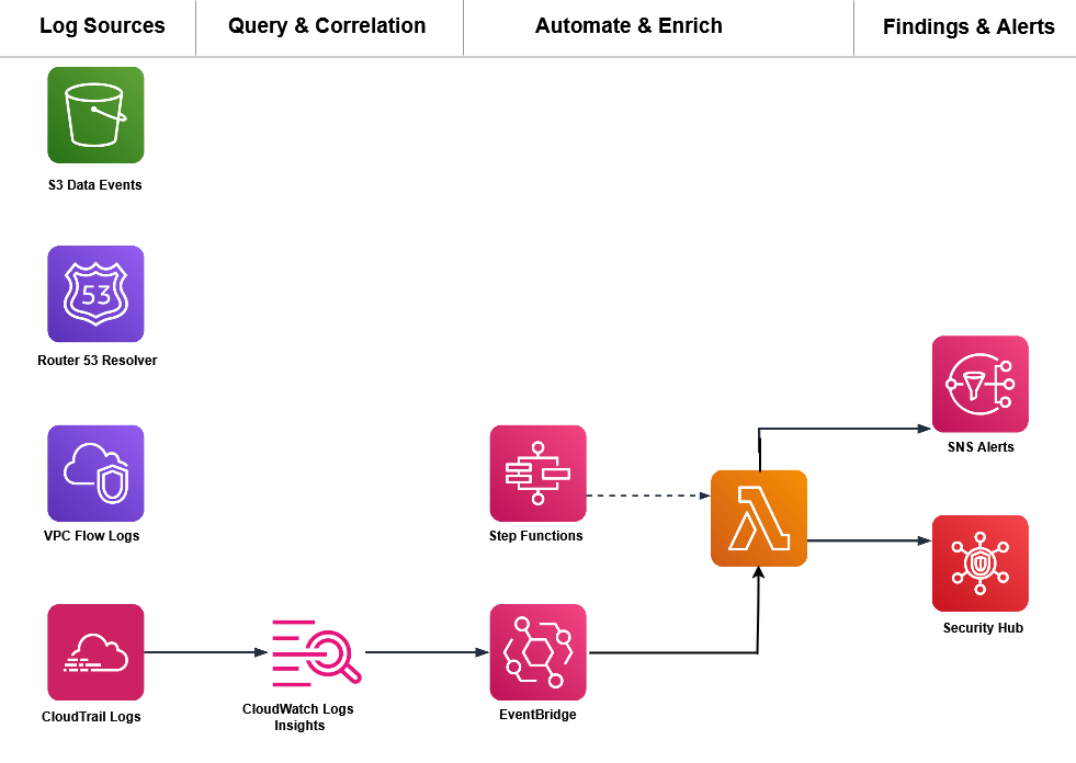
As your library grows, move the logic into automated pipelines with EventBridge, Lambda, and AWS Step Functions (a serverless orchestration service that coordinates multiple services into workflows), and surface correlations next to findings in Security Hub. For cross-service correlation at scale, CloudWatch unified data and telemetry capabilities can convert security and compliance data into the OCSF format and let you query sources such as CloudTrail, VPC Flow Logs, and DNS logs from one interface. Security Lake with Athena is a strong option for long-term analysis. Choose the endpoint that fits your retention and query needs.

Figure 3 shows a correlation pipeline built on AWS services including EventBridge, Lambda, Step Functions, and AWS Security Hub. The pipeline runs from data sources through scheduled queries and enrichment to automated response and centralized visibility.

Figure 3: A correlation pipeline built on AWS services

Figure 3: A correlation pipeline built on AWS services

Conclusion

You now have four correlation patterns that layer your business context on top of GuardDuty Extended Threat Detection to catch attacks specific to your environment. A few principles carry across every correlation you build.

  • Identity is your primary correlation key: Track the same principal across services.
  • Time windows matter, but they depend on the attack: Events minutes apart are usually related for fast, automated sequences; the ten-minute bins here work for that pattern. Slow or manual reconnaissance can stretch across hours or days, so widen the window when the pattern is deliberate rather than automated.
  • Context is what you add: Your data classification, access norms, resource ownership, and change windows are signals you bring to detection.
  • Start with one rule: A single well-tuned correlation catches more significant activity than a wall of uncorrelated alerts.

GuardDuty Extended Threat Detection handles the multi-stage patterns common across customers. The correlations in this post add the layer that only your business context can supply. Start with one pattern this week, validate it against your own traffic, and add the next pattern after the first proves reliable.

Have you built correlation rules for patterns not covered here? Share your experience in the Comments section below.

Further reading
 

Nisha Kashyap

Nisha Kashyap

Nisha Kashyap is a Senior Support Security Engineer at AWS. She works on threat detection and security operations, helping customers investigate security events and build detection that connects signals across AWS services and reflects their own environment.

Gallup scales real-time coaching for thousands with Amazon Bedrock

Post Syndicated from Tamil Sambasivam original https://aws.amazon.com/blogs/architecture/gallup-delivers-real-time-workplace-coaching-to-thousands-of-leaders-with-amazon-bedrock/

How Gallup turned 90 years of workplace science into an AI assistant that gives leaders personalized guidance in seconds, powered by Amazon Bedrock.

Gallup delivers analytics and advice to help leaders and organizations solve their most pressing problems. With more than 90 years of experience and a global reach, Gallup has developed a uniquely deep understanding of workplace behavior and performance.

However, this knowledge wasn’t centralized or delivered in context. Leaders had to navigate multiple resources to find relevant insights and then translate them into action without guidance. The lack of real-time, personalized recommendations meant workplace challenges were often handled reactively instead of proactively.

Gallup needed to transform decades of proprietary research into real-time, personalized guidance that leaders can access instantly within their existing workflow.

In this post, we show how Gallup built Gallup AI, a generative AI assistant powered by Amazon Bedrock. It transforms decades of proprietary workplace research into real-time, personalized coaching delivered directly within the Gallup Access application.

Why Amazon Bedrock

Gallup evaluated multiple approaches to building a generative AI assistant. The team chose Amazon Bedrock for three reasons:

  1. Access to leading foundation models like Anthropic’s Claude without managing infrastructure.
  2. Built-in retrieval augmented generation (RAG) through Amazon Bedrock Knowledge Bases, a fully managed RAG capability, grounds responses in verified research.
  3. Native guardrails to enforce content safety at scale.

This combination allowed Gallup to move from prototype to production in weeks rather than months, without hiring a dedicated machine learning (ML) operations team.

Note: Anthropic’s Claude models on Amazon Bedrock are available in select AWS Regions. For current model and Region availability, see Supported models by Region in Amazon Bedrock.

The approach: Building intelligence into daily workflow

Gallup built Gallup AI, a generative AI-powered assistant integrated directly into Gallup Access. The unified application lets managers review engagement results, build action plans, explore CliftonStrengths insights, and access curated content to better support their teams.

The solution uses Amazon Bedrock with Anthropic’s Claude models to deliver conversational insights grounded in Gallup’s proprietary research. Amazon Bedrock Knowledge Bases and Amazon Kendra retrieve relevant research and organizational data. This is designed to ground responses in verified workplace science. Amazon Bedrock Guardrails enforce content safety policies, while AWS Lambda with FastAPI delivers real-time streaming responses that feel natural and immediate.

The architecture follows a serverless design and supports multiple organizations simultaneously. Amazon ElastiCache Serverless provides sub-millisecond response times for conversation history. Amazon Relational Database Service (Amazon RDS) for MySQL serves as the durable system of record. Amazon Data Firehose streams usage metrics to Amazon Simple Storage Service (Amazon S3) for cost management and performance optimization.

How the solution works

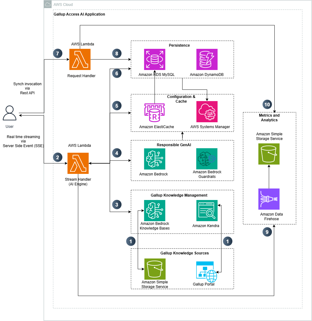
The following diagram shows the Gallup Access AI application architecture.

Architecture diagram of the Gallup Access AI application showing request flow through AWS Lambda to Amazon Bedrock, with Amazon Bedrock Knowledge Bases and Amazon Kendra for retrieval, Amazon ElastiCache Serverless and Amazon RDS for storage, and Amazon Data Firehose streaming metrics to Amazon S3

Figure 1: Gallup Access AI application architecture

The architecture processes requests through the following stages:

Gallup’s proprietary workplace research covers decades of employee engagement studies, performance data, and organizational insights. The content is stored in Amazon S3 and ingested into Amazon Bedrock Knowledge Bases. The application also continuously crawls the Gallup website to capture the latest research publications, articles, and insights, indexing this content in Amazon Kendra for instant retrieval. This dual approach gives the AI assistant access to both historical research archives and current workplace science, delivering responses grounded in verified, up-to-date knowledge rather than generic advice.

When a leader asks Gallup AI a question, the system retrieves relevant research from both Amazon Bedrock Knowledge Bases and Amazon Kendra. The system scores documents based on confidence thresholds, filters them, and consolidates them before sending them to Claude models in Amazon Bedrock.

The conversation flows through AWS Lambda handlers that manage both real-time streaming (for web clients) and synchronous requests (for backend services). Amazon ElastiCache Serverless caches recent conversation history for instant retrieval, while Amazon RDS for MySQL serves as the durable storage layer with organized records of conversations, prompts, responses, and source citations.

Amazon Bedrock Guardrails apply content safety policies during generation, with the ability to intervene mid-stream if policy violations are detected. Interactions persist before streaming begins, preserving transactional integrity even if connections are interrupted.

AWS Systems Manager Parameter Store serves as the application’s centralized configuration hub, managing AI model settings, content safety policies, and performance thresholds. This allows the team to adjust application behavior instantly, without redeploying code or interrupting service for users.

Amazon DynamoDB provides fast, flexible storage for product-specific insights and contextual data, so the application delivers personalized experiences tailored to each user’s role and workflow.

Comprehensive metrics, including I/O tokens, cached tokens, time-to-first byte, and stop reasons, flow through Amazon Data Firehose to Amazon S3, providing visibility into cost, performance, and usage patterns across the application.

What Gallup has achieved

Gallup has transformed decades of workplace research into an intelligent assistant that delivers measurable value across thousands of organizations. Tasks that previously required navigating reports, articles, and tools now resolve through a single conversational interaction. Time to insight dropped from manual research to real-time, AI-delivered guidance within seconds. The application processes billions of tokens through production interactions, with responses grounded in verified workplace science.

Since launching in June 2024, adoption and engagement have grown rapidly:

Metric Result
Prompts Increased ~7x
Conversations Increased ~4.5x
Active users Increased ~5.5x
Engagement depth Average prompts per conversation increased ~55%, indicating sustained, multi-turn interactions
Response latency Sub-second time-to-first byte (TTFB) for streaming responses. Sub-millisecond session retrieval via Amazon ElastiCache Serverless

What the customer said

Gallup’s Director of Product reflects on what this shift means for how leaders access workplace science:

“Gallup AI represents a fundamental shift in how leaders access workplace science. For decades, our research helped organizations make better decisions, but it often required leaders to search, interpret, and apply those insights themselves. By building on Amazon Bedrock, we’re embedding scientifically grounded guidance directly into the flow of work, giving managers real-time support that is both personalized and actionable.”

— Andrew Bridger, Director of Product, Gallup

With this foundation in place, Gallup is focused on expanding what the application can do next.

What’s next

Gallup’s roadmap focuses on making its expertise more accessible, actionable, and embedded into everyday workflows. A key initiative is the development of an AI-curated prompt library that captures the most common questions managers and leaders ask. This library will help users quickly engage with Gallup AI through proven, high-value prompts grounded in workplace research.

In addition, Gallup is introducing guided coaching experiences built around structured conversation flows. These guided prompts walk managers through well-defined coaching scenarios, such as improving engagement, addressing team challenges, or developing employees, by sequencing prompts and responses into purposeful, outcome-driven interactions.

Gallup is building an agent-based foundation using Amazon Bedrock AgentCore. This positions Gallup AI to move beyond a user-facing assistant. By surfacing tools, workflows, and proprietary knowledge programmatically, the system can support not only end users but also other systems and integrations across the application.

Conclusion

By combining the generative AI capabilities of Amazon Bedrock with Gallup’s proprietary workplace research, leaders now have instant access to scientifically grounded guidance exactly when they need it. The serverless architecture enables the application to scale reliably while delivering low-latency streaming responses and comprehensive observability.

To build your own generative AI application, get started with Amazon Bedrock. To learn more about grounding responses in your own data, explore Amazon Bedrock Knowledge Bases.

Further reading

About the authors

Closing the AI agent trust gap with graduated autonomy

Post Syndicated from Dev Arora original https://aws.amazon.com/blogs/architecture/closing-the-ai-agent-trust-gap-with-graduated-autonomy/

How much to trust an AI agent is now a daily operational question. Agents read customer data, open tickets, process refunds, and delete accounts, yet most teams pick up a binary: full access or read-only. Full access is risky because agents fail unpredictably. Read-only leaves most of the agent’s value unused. The distance between what an agent could do and what an operator trusts it to do is the agent’s trust gap.

In this post, we describe graduated autonomy, an architectural pattern that closes the gap. Agents earn expanded permissions through sustained reliability and lose them when performance degrades. Amazon Bedrock AgentCore, a platform to build, connect, and optimize agents at scale with any framework or model, provides the runtime, gateway, policy, and evaluation capabilities. Amazon DynamoDB stores trust state. AWS CodePipeline gates delivery on evaluation results. We cover each layer’s responsibility and the key design decision behind it.

The agent trust gap

Identity and access management answers “who can do what?” once, at provisioning. That model assumes that the principal behaves consistently. A large language model agent breaks it: the same agent can be accurate Monday and hallucinated Tuesday after a prompt change or model update.

Closing the gap requires three capabilities raw API logs rarely provide:

  • Visibility. API logs tell engineers what happened but tell a compliance officer nothing about whether an action was safe.
  • Decision provenance. Tracing an action back to the signal that triggered it, the alternatives considered, and the confidence held.
  • Reversibility. Pre-action state capture, so operators can recover from incorrect actions.

The framework that implements this pattern delivers all three through six architectural layers.

Solution overview

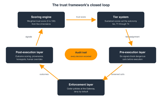
The six layers:

  • Scoring engine computes trust from configurable dimensions.
  • Tier system translates sustained scores into autonomy levels.
  • Pre-execution layer blocks dangerous actions before they run.
  • Enforcement layer applies tiers through Cedar policies at the infrastructure level.
  • Post-execution layer evaluates outcomes, records of provenance, and feeds signals back to scoring.
  • Delivery gate keeps degraded agent versions out of production.
Architecture diagram of the trust framework as a clockwise closed loop: the scoring engine produces a weighted trust score from five dimensions, the tier system converts sustained scores into autonomy tiers T1 through T4, the pre-execution and enforcement layers apply the current tier through in-process checks and Cedar policies, and the post-execution layer returns outcome scores, honeypot results, and human overrides to the scoring engine, with an audit trail at the center recording every decision.

Figure 1: The trust framework’s closed loop.

Each layer is replaceable: the scoring model, tier thresholds, pre-execution signals, and evaluation criteria are configuration, not code. Each layer also embodies one deliberate design decision, developed in the following sections:

Layer Key design decision
Scoring engine Safety is an independent floor, never averaged away by strong metrics
Tier system Start every agent at T1. Promote slowly, demote immediately
Pre-execution layer Fast in-process filters are backstopped, never solely trusted
Enforcement layer Deny by default, enforced outside the agent’s process
Post-execution layer Audit records capture pre-action state, making recovery possible
Delivery gate One unauthorized tool call in adversarial tests blocks release

The scoring engine

The scoring engine computes a weighted score from 0 to 100 per agent over a rolling window of 50 actions, from five dimensions:

Dimension Weight What it measures
Accuracy 25% Task completion correctness against expected outcomes
Safety 20% Boundary respect, adversarial content detection, permitted tool adherence
Consistency 20% Behavioral predictability, inverse of tool-use pattern drift
Compliance 20% Reasoning quality before acting, guardrail adherence
Efficiency 15% Execution without unnecessary retries or resource waste

The composite drives dashboards and tier assignment, but safety acts as an independent floor, so a dangerous individual metric never hides strength elsewhere.

The tier system

Every new agent starts at T1, regardless of test performance:

Tier Score range Permissions
T1: Probation 0 to 40 Read and list only. Two tools visible.
T2: Supervised 41 to 70 Add write operations. Human approves high-risk.
T3: Trusted 71 to 90 Execute and modify. Anomalies flagged for review.
T4: Autonomous 91 to 100 Full access. Post-hoc audit only.

Three rules govern transitions:

  • Promotion requires sustained performance. The score must stay above the promotion threshold for the entire rolling window.
  • Demotion is immediate. When safety drops below its floor or injection is detected, the agent moves down.
  • Hysteresis prevents oscillation. Promotion into a tier requires a score 5 points above that tier range floor. Demotion happens at the range floor itself. An agent at a boundary cannot flap between tiers.

Trust state lives in Amazon DynamoDB as a current state record plus a time-series history per agent. Enforcement components read the current tier on every invocation, a lookup DynamoDB typically serves in single-digit milliseconds.

The pre-execution layer

Post-execution evaluation cannot undo damage, so the pre-execution layer evaluates every tool’s call and can block it before execution. It scores six signals independently:

  • Adversarial injection detection. Pattern matching against known injection phrases. One match triggers an instant block and a trust penalty.
  • Sensitive target detection. Regex matching credentials, tokens, and private keys in tool arguments.
  • Dangerous tool detection. Flagging tools that match destructive operation patterns.
  • Behavioral consistency. Comparing the current tool call against the agent’s historical tool-use distribution.
  • Confidence calibration. Comparing stated confidence against historical accuracy. Overconfident failures are penalized at twice the normal rate.
  • Reasoning quality. Checking whether the agent provided reasoning before acting.

These checks are fast first-pass filters, not a complete defense. The enforcement layer’s deny-by-default policies backstop anything they miss.

The enforcement layer

The pre-execution layer is application code inside the agent’s process. The enforcement layer operates outside the agent, at the infrastructure level.

AgentCore Gateway, a capability of Amazon Bedrock AgentCore, sits between the agent and its tools. It routes every MCP tool invocation through Policy in Amazon Bedrock AgentCore, which evaluates Cedar policies with forbid-wins semantics. One satisfied forbid overrides any number of permits. Tier maps to policy state:

  • Probation: A forbid policy blocks write, execute, and delete tool actions.
  • Promotion: The forbid policy is removed, and broader permits take effect.
  • Demotion: The forbid policy is re-applied.

With the policy engine in enforce mode, the Gateway lists only tools that policy could permit, so the tier’s unconditional forbids keep blocked tools out of the listing. The agent is unlikely to call a tool it has never seen. Listing is a meta-action: each invocation is still evaluated separately with full request context, including input parameters. Cedar denies by default. Enforcement never depends on the agent’s choosing to behave. For model-level content safety, Amazon Bedrock Guardrails complements Policy in AgentCore, filtering harmful content and masking sensitive information independent of tier.

The post-execution layer

After every tool call, the system scores the outcome across eight signals, from confidence calibration and behavioral drift to human overrides and retry detection. Every action generates an audit record following the Think, Plan, Act, Observe, Score chain:

  • Think: The agent’s reasoning chain.
  • Plan: Tool selected, input prepared, pre-execution score.
  • Act: Cedar policy matched, Gateway route processed.
  • Observe: Success or failure, output data.
  • Score: Trust impact, per-dimension scores, tier change.

The Plan and Act records capture pre-action state, which is what makes recovery from an incorrect action possible. Operators ask questions in plain English, and a provenance query endpoint returns a human-readable explanation of any decision. Audit entries persist to DynamoDB.

The delivery gate

Each change to the agent’s prompt, configuration, or tool definitions triggers an AWS CodePipeline run. The run deploys the candidate to staging and runs it against ground-truth fixtures with Amazon Bedrock AgentCore Evaluations, a capability of Amazon Bedrock AgentCore. The fixtures include adversarial cases such as prompt injection and data-exfiltration requests. A single unauthorized tool call in any adversarial case fails the gate. The version that passes becomes the last known stable version.

Production monitoring and recovery

The framework injects synthetic honeypot cases with known expected behavior into a small share of traffic. Validation checks the tool-call trajectory (expected tools, expected order, no forbidden tools) rather than nondeterministic natural-language output, so a mismatch signals a real anomaly. Honeypot results stay out of production metrics. When safety drops below the floor, demotion narrows the agent’s permissions, and the framework redeploys the last known stable version. Together they restore known-good code alongside a tighter permission set. The framework also alerts operators.

Operator judgment feeds directly: the rolling rate at which operators reject proposed actions caps the effective safety metric, so 30 percent rejections cap safety at 70. An emergency stop pushes a single Cedar deny-all policy. Once the policy is active, typically within seconds, the Gateway denies all tool invocations without a redeployment. In multi-agent systems, a delegated action’s effective tier is the minimum across the delegation chain, closing the delegation privilege-escalation path.

Conclusion

In this post, we described graduated autonomy, an architectural pattern for closing the agent trust gap. With this pattern in place, your agents hold the autonomy their track record supports.

To get started, take the dimension weights and tier boundaries from the two tables in this post as a starting template for one agent in your fleet. Start that agent at T1. Then follow the Amazon Bedrock AgentCore Evaluations documentation to build the delivery gate, and the Policy in Amazon Bedrock AgentCore documentation to write the tier policies. You can explore these capabilities in the Amazon Bedrock console and on the Amazon Bedrock AgentCore detail page.

For deeper dives into the building blocks this pattern uses, read Secure AI agents with Policy in Amazon Bedrock AgentCore and Build custom code-based evaluators in Amazon Bedrock AgentCore.


About the authors

Amazon MSK Service 101: How many partitions does an Amazon MSK topic need?

Post Syndicated from Yashika Jain original https://aws.amazon.com/blogs/big-data/amazon-msk-service-101-how-many-partitions-does-an-amazon-msk-topic-need/

Customers new to Amazon Managed Streaming for Apache Kafka (Amazon MSK) often ask how many partitions their topics need. Choosing the right partition count is one of the most impactful architectural decisions you make, because it directly affects throughput, scalability, and operational complexity.

In Apache Kafka, a topic is the fundamental unit for categorizing data streams, but to achieve high scalability and performance, Kafka divides topics into smaller, independent units called partitions.

In this post, we provide practical guidance for determining the ideal partition count for your use case.

Understanding Kafka partitions

In
Apache Kafka, a partition is the unit of storage and parallelism. Each partition is an ordered, immutable log that can store records as they are produced to a topic. When you create a topic, Kafka distributes its partitions across the brokers in the cluster. Partitions allow Kafka to scale in three key ways:
  • Parallelism – Within a consumer group, each partition can be read by only one consumer at a time. Each partition maps to a dedicated log file in storage on the broker, and Kafka manages these logs through separate processing threads. This architecture allows more partitions to support more consumers processing data in parallel, with each partition’s log being independently managed for read and write operations.
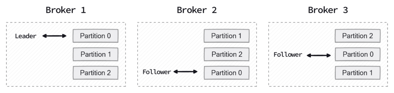
The following diagram shows how Kafka distributes partition replicas across a three-broker cluster, with each broker serving as a leader for some partitions and a follower for others.
Partitions 0, 1, and 2 replicated across three brokers, each a leader for some partitions and a follower for others

Figure 1: Partition replicas distributed across a three-broker cluster

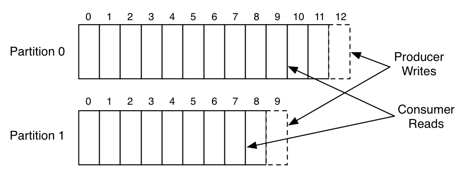
The following diagram illustrates how producers append new records to the end of a partition log, while consumers read sequentially from their current offset position.

Producers append records to the tail of partition logs while consumers read sequentially from their offset position

Figure 2: Producer writes and consumer offset positions in two partition logs

  • Throughput – Producers and consumers can read and write data in parallel across partitions, increasing overall throughput.
  • Scalability – Partitions allow Kafka to spread data and load across multiple brokers instead of concentrating it on a single node.

However, increasing partitions comes with trade-offs. Each partition adds metadata overhead, consumes memory, and requires file handles on the broker. While more partitions improve throughput and parallelism, they also increase the operational burden on the cluster. Too many partitions can lead to longer leader election times during broker failures, increased end-to-end latency, and higher memory consumption for both producers and consumers managing connections to multiple partitions.

Trade-offs when choosing partition count

Choosing a partition count is a balancing act between parallelism and resource utilization.

Benefits of more partitions

Using more partitions can significantly improve throughput by allowing Kafka to distribute read and write traffic across more brokers. This is particularly useful for high-volume ingestion pipelines and real-time analytics workloads. More partitions also allow consumer groups to scale horizontally, because the maximum number of active consumers in a group is limited by the number of partitions. In addition, choosing a partition count that is evenly divisible by the number of brokers helps provide balanced leadership and replica distribution, reducing the risk of uneven load.

Operational costs of more partitions

However, higher partition counts also come with costs. When a broker fails or undergoes maintenance, Kafka must perform recovery operations for each affected partition. During recovery, Kafka elects new leaders for partitions that were hosted on the unavailable broker and replicates data from the remaining in-sync replicas to newly assigned brokers. This process involves copying partition data across the network to restore the replication factor, which can be resource intensive. As the number of partitions increases, these recovery operations take longer because each partition requires its own leader election and data replication cycle.

You might encounter clusters with very high partition counts that experience extended recovery times during rolling upgrades, even when overall traffic volumes are modest. Amazon MSK Express brokers address this challenge by recovering 90x faster and providing 180x faster elasticity when scaling out clusters. This significantly reduces the operational impact of high partition counts during maintenance windows and failure scenarios.

Infrastructure cost implications

Beyond operational complexity, more partitions can directly increase infrastructure costs. Amazon MSK publishes partition-per-broker limits that vary by instance type. When the total partition count (including replicas) exceeds what the current broker fleet can support, you must add brokers to stay within recommended limits, even if throughput alone does not warrant the additional capacity.

Amazon MSK partition-per-broker guidelines

Amazon MSK publishes recommended partition-per-broker guidelines to help you operate clusters reliably. These values are strict limits. Exceeding them can lead to operational challenges, particularly during broker replacement or rolling upgrades, and can block cluster operations such as configuration updates or scaling down.

Express brokers support up to 5x more partitions per broker compared to Standard brokers. For example, the largest Standard broker (kafka.m7g.16xlarge) supports a recommended maximum of 4,000 partitions per broker. The equivalent Express broker (express.m7g.16xlarge) supports up to 20,000 recommended partitions per broker. This higher partition density means partition-bound workloads can be hosted on fewer brokers, improving price-performance by up to 50% for such workloads.

We recommend setting Amazon CloudWatch alarms on PartitionCount per-broker metrics to proactively monitor your partition distribution. When an alarm triggers, evaluate your partition strategy and consider rebalancing partitions across brokers, consolidating topics, or scaling out your cluster to stay within recommended limits. For detailed guidance, see Right-size your cluster: Number of partitions per Standard broker and Express broker partition quota.

Practical guidance for choosing a partition count

There is no single formula that works for every Kafka workload. In practice, you typically combine several considerations when sizing partitions.

  • Start with throughput requirements – The first step is to determine your per-partition throughput capacity, which then informs how many partitions you need.

For Express brokers, use the per-broker throughput capacity as the primary means for sizing your cluster. Express brokers feature a fully managed storage layer, so you do not need to separately account for storage I/O constraints. The published per-broker limits represent the effective capacity available to your workload.

For Standard brokers, the achievable throughput depends on additional factors beyond the broker instance size. These factors include provisioned EBS storage throughput, the number of consumer groups reading from the broker, and how much data is served from memory versus disk. Storage I/O is consumed when producers write, when data replicates between brokers, and when consumers read data that is not in memory. For this reason, validate the effective per-partition throughput for Standard brokers through load testing in your environment.

Once you know your per-partition throughput, calculate the required number of partitions: Number of partitions = Peak throughput of the topic ÷ Throughput per partition

For example, if a topic must handle 40 MB/sec at peak and your testing shows each partition can sustain 5 MB/sec, you would need: 40 ÷ 5 = 8 partitions. Always validate these assumptions with load testing, as actual throughput varies based on your workload characteristics. For initial sizing estimates, refer to the Amazon MSK Sizing and Pricing worksheet and the Amazon MSK Best Practices documentation.

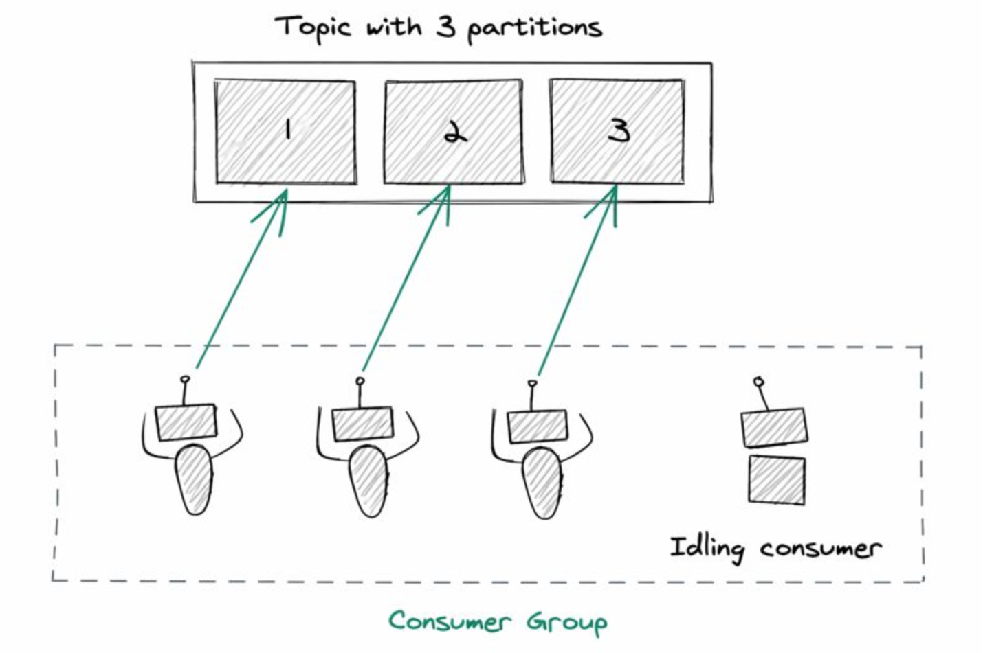
  • Consider your consumer parallelism needs – If you know the number of consumers required during peak processing times, use that as your partition count. We don’t recommend having more active consumers in a consumer group than partitions. For example, if you have 5 partitions, only 5 consumers can actively process data. Additional consumers remain idle. These idle consumers still maintain active TCP connections to the brokers, sending frequent heartbeats and group coordination requests. This might result in unnecessary overhead on broker resources and contribute to high CPU usage despite low egress traffic.
Consumer group with more consumers than partitions, leaving the extra consumers idle

Figure 3: Idle consumers when a consumer group has more consumers than partitions

  • Producer throughput and partition keys – When sizing partitions, consider producer-side throughput in addition to consumer parallelism. If producers generate data faster than a single partition can handle, additional partitions can help distribute write traffic across brokers. Partition keys also play a critical role. Poorly distributed or low-cardinality keys can create hot partitions and limit throughput. In such cases, increasing the number of partitions alone does not improve throughput unless records are evenly distributed.
  • Plan for even distribution and future growth – Kafka works best when partitions can be spread evenly across brokers. Instead of focusing on specific numbers, aim for partition counts that divide reasonably well across your expected broker count. This reduces reassignment churn when brokers are added or replaced. But avoid excessive over-partitioning. It’s reasonable to leave some headroom for future growth. However, creating thousands of partitions “just in case” often causes more harm than good. Increasing partitions later is supported, but it can affect ordering guarantees and may require consumer changes. Start with a conservative number, monitor real traffic patterns, and scale gradually.

From an operational perspective, Amazon MSK provides recommended partition-per-broker guidelines based on broker instance type. Exceeding these guidelines increases operational risk and can block cluster operations such as version upgrades, scaling, or configuration changes. Large partition counts can also increase consumer group rebalance duration, temporarily pausing message processing and increasing end-to-end latency.

Keep in mind that partitioning improves scalability, but it does not address application-level bottlenecks such as slow consumers, inefficient processing logic, or downstream system constraints.

Conclusion

Determining the right number of partitions for an Amazon MSK topic is a foundational design decision. It affects throughput, scalability, failure recovery, and day-to-day operability of your Kafka cluster. Start by understanding your throughput and consumer parallelism needs, respect Amazon MSK partition-per-broker guidelines, avoid excessive over-partitioning, and validate assumptions through load testing. Most importantly, there is no universal “correct” number, only a number that fits your workload, operational goals, and cost.

For more information, see the Amazon MSK Developer Guide and Recommended best practices for Amazon MSK.


About the authors

Yashika Jain

Yashika Jain

Yashika is a Senior Cloud Analytics Engineer at AWS, specializing in real-time analytics and event-driven architectures. She is committed to helping customers by providing deep technical guidance, driving best practices across real-time data platforms and solving complex issues related to their streaming data architectures.

Ali Alemi

Ali Alemi

Ali is a Principal Streaming Solutions Architect at AWS. Ali advises AWS customers with architectural best practices and helps them design real-time analytics data systems which are reliable, secure, efficient, and cost-effective. Prior to joining AWS, Ali supported several public sector customers and AWS consulting partners in their application modernization journey and migration to the Cloud.

[$] An ongoing 3D-printer AGPL violation

Post Syndicated from jake original https://lwn.net/Articles/1089390/

At FOSSY 2026, several people from the
Software Freedom Conservancy (SFC),
which organizes the conference, gave a presentation about an ongoing
violation
of the Affero General Public
License version 3
(AGPLv3). Bradley Kühn, Karen Sandler, and Denver
Gingerich spoke about different aspects of the violation, which is in
regard to 3D-printer software from Bambu Lab, and what is being
done to try to provide users with alternatives. One aspect that is
particularly interesting is that the circumvention that the company is
employing is precisely what the AGPL was written to prevent.

Armbian 26.8 released

Post Syndicated from jzb original https://lwn.net/Articles/1090741/

Version 26.8 of
the Armbian distribution for Arm hardware has
been released.

Most releases are a long list of small improvements. This one had three
larger pieces landing at roughly the same time, and all three touch parts of
Armbian that people use directly rather than parts they only read about in
changelogs.

The installer was rewritten. Armbian Imager reached 2.0. And our CI moved out
of the repository it had outgrown into one built for the job. None of these were
planned to coincide; they simply reached the point where postponing them again
would have cost more than doing them.

The installer rewrite is the one I expect people to notice first. It now
ships as an armbian-config module, which means it is unit-tested, the same way
the rest of armbian-config is tested, rather than living as a script that
everyone was slightly afraid to touch. It can target SPI and MTD, treats eMMC
and NVMe as separate flows instead of pretending they are the same thing, can
flash a bootloader on its own, and — this one is overdue — reports when a
bootloader write fails instead of printing “Done.” and leaving you to find out
at the next boot.

See the release notes
for a full list of changes.

AWS and DuckLabs: Building the future of analytics together

Post Syndicated from Mai-Lan Tomsen Bukovec original https://aws.amazon.com/blogs/big-data/aws-and-ducklabs-building-the-future-of-analytics-together/

Today we are announcing that Amazon has signed a definitive agreement to acquire DuckLabs, the Amsterdam-based company behind the open-source analytical database DuckDB. We expect the transaction to close shortly, subject to customary closing conditions. Hannes Mühleisen and Mark Raasveldt, who created DuckDB and co-founded DuckLabs, will continue leading the team and the open-source project’s technical direction as part of AWS. The DuckDB open-source project will also continue to be driven by the DuckLabs team, remain open source under the independent Foundation (the non-profit that oversees DuckDB), and available under the MIT license as it does today (see DuckLabs blog).

Data has always been a core asset and differentiator for companies. That is true now more than ever, as organizations use their data to customize inference and build AI agents. For 20 years AWS has driven the frontier of data, starting with the launch of Amazon S3 to create data lakes for every business, the first cloud analytics service in Amazon EMR, the first cloud data warehouse with Amazon Redshift and the many capabilities that we have introduced with Athena, Glue ETL, etc. We continue innovating for AWS customers on the data frontier including providing Apache Iceberg capabilities directly in S3 Tables, vector storage in the data lake and our new optimized Graviton-based Redshift clusters.

DuckDB has also been at the forefront of changing how the world works with data. Hannes and Mark started DuckDB while at Centrum Wiskunde & Informatica (CWI), the national research institute in the Netherlands that also invented Python. The founders of DuckDB realized that older databases and analytics engines like Spark focused on performance for very large data processing but didn’t have an effective way to “scale down” to smaller size data queries that form the backbone of what most customers do with SQL analytics.

DuckDB set out to solve the problem of blazingly fast performance for the 90%+ of data queries in the world today, that often runs 1 terabyte of data or less as part of analysis and dashboarding. DuckDB’s architecture is based on that core premise of “make the everyday SQL query super fast” so DuckDB runs in-process to other applications which simplifies and speeds up data exchange with the application. DuckDB gets big performance gains from its vectorized execution because it does not require a heavy compiler to run simple statements like SELECT * FROM table. And what works for everyday queries also (unsurprisingly) works very well for agents because agents behave a lot like people when interacting with data. They poke. They experiment. They run exploratory analysis on small data sets before figuring out what they really want to do. DuckDB ends up being naturally optimized for AI agents to use. What started as an academic project is now widely adopted across data engineering, data science, analytics, and now AI agents, for its simplicity of use and raw performance. We plan to combine the superpower of DuckDB at everyday queries of a terabyte or less with the proven exabyte-plus enterprise scale of S3 and our AWS analytics services of Redshift, Athena, EMR, Glue-ETL, and SageMaker platform which power analytics across hundreds of terabytes to petabyte of data. Andy Warfield, Distinguished Engineer at AWS, talks about DuckDB and the Changing Physics of Analytics in Werner Vogel’s All Things Distributed blog.

Our customers use DuckDB today with AWS services and tell us how much they love it for its speed and simplicity. For example, DuckDB today executes SQL directly against external files, such as Parquet, CSV, and JSON, stored locally or on cloud storage like S3 for unparalleled performance and significantly lower cost. DuckDB can also run in-process to AWS Lambda functions.

David Feng, Executive Director, Scientific Computing at Allen Institute, said “The Allen Institute accelerates science for a healthier world by tackling the biggest questions in biology at a large scale, and that involves extensive analysis of large, multimodal data. We started using DuckDB to analyze terabytes of scientific data in 2025 and love it. We are storing data in S3 for realtime quality control and analysis of neurophysiology and behavior data, critical to driving the next data acquisition. Queries that took minutes now come back in less than a second, enabling completely new ways of interacting with data.”

We are excited to make DuckDB applications run best on AWS, and will continue to invest in deep integration between DuckDB and our building block services.

We are also using DuckDB in our own AWS infrastructure. When Amazon Quick wanted to augment the performance of their custom dashboarding engine, they picked DuckDB to query data in S3 Tables. The Quick team found that the DuckDB engine scales effortlessly with the number of CPUs, and its single library can easily plug into the internal Quick control plane subsystems. Since we launched Quick in October 2025, we have processed over 2.5B queries using our custom Quick query engine with the DuckDB integrations and optimizations. These DuckDB integrations and optimizations helped Amazon Quick reduce average query latency by 30%. We are going to look at how we can integrate DuckDB’s performance and simplicity in our other AWS services across data and analytics.

Stay tuned for more about how DuckLabs and AWS will reinvent the frontier of data together for applications, data engineers, and AI, meeting customers where they are today and giving them the benefits of DuckDB’s innovation within AWS.


About the author

Mai-Lan Tomsen Bukovec

Mai-Lan Tomsen Bukovec, Technology Vice President at AWS, leads the Amazon cloud data services that millions of AWS customers rely on for digital transformations, business analytics, machine learning, generative AI, and next generation customer experiences. With over 25 years of experience in the technology industry, Mai-Lan is a pioneer in helping customers take advantage of cloud-based technologies to transform their businesses.

Security updates for Wednesday

Post Syndicated from jzb original https://lwn.net/Articles/1090732/

Security updates have been issued by AlmaLinux (firefox, gstreamer1-plugins-base, kernel, kernel-rt, and sqlite), Debian (freecad, kernel, libvncserver, and openssl), Fedora (apr-util, chromium, nnn, perl-DBI, python-tablib, python3.10, python3.11, python3.12, and sympa), Gentoo (DTrace, GNU screen, UnrealIRCd, and Vinyl Cache), Oracle (389-ds-base, attr, firefox, gegl04, grafana, gstreamer1-plugins-base, gstreamer1-plugins-good, httpd, mod_http2, nginx, pam, python-pyasn1, python-urwid, python3.12, python3.14, sqlite, and xorg-x11-server), SUSE (amazon-ecs-init, containerd, curl, distribution, dracut, ffmpeg-7, fuse-overlayfs, gd, git-lfs, go1.25-openssl, go1.26-openssl, govulncheck-vulndb, hauler, himmelblau, kernel, librest, libssh2_org, open-iscsi, openssh, patch, perl-Date-Manip, podman, postgresql14, postgresql16, python-cryptography, python-Pillow, python311, rmt-server, rootlesskit, rpm, rsync, runc, snpguest, sssd, suseconnect-ng, unbound, and util-linux), and Ubuntu (curl, ffmpeg, linux-aws-6.8, linux-azure-fde, linux-azure-fde-6.8, linux-azure-fips,
linux-nvidia-tegra, linux-azure, linux-azure-fde, linux-azure, linux-azure-fde, linux-nvidia-tegra-igx, linux-azure-5.4, linux-azure-fips, linux-oracle, linux-raspi, linux-raspi-realtime, openjdk-17, openjdk-21, openjdk-25, openjdk-8, openjdk-lts, openssl, perl, and vim).

AI-driven software delivery with Kiro, AWS DevOps Agent and Bluebox by Dynatrace

Post Syndicated from Philipp Ushiromiya original https://aws.amazon.com/blogs/devops/ai-driven-software-delivery-with-kiro-aws-devops-agent-and-bluebox-by-dynatrace/

This post was co-written with Michael Stephan, Senior Principal Product Manager, and Christian Kreuzberger, Principal Software Engineer, at Dynatrace.

AI-driven software delivery changes how code gets written, but not what production demands of it. A generated change still has to fit the traffic your service receives, the dependencies it calls, and the capacity limits it runs within. Without that context, you validate the change after it ships, which adds rework and deployment risk.

Kiro turns intent into specifications, code, and pull requests. AWS DevOps Agent investigates incidents and proposes mitigations. Bluebox by Dynatrace supplies the runtime topology, dependency, and traffic data that both draw on, so each change and each investigation is grounded in how the system behaves rather than how it’s expected to behave. In this post, we will follow a travel-booking example from feature design through post-deployment remediation. You’ll see how telemetry from Bluebox shapes a change in Kiro, how AWS DevOps Agent investigates an incident, and where human review and existing CI/CD controls remain in the process.

What are Kiro and AWS DevOps Agent?

Kiro is an agentic development environment that applies AI across the software development lifecycle. Its spec-driven workflow organizes a feature request into requirements, design, and implementation tasks before generating any code.

AWS DevOps Agent is a frontier agent for software delivery and operations across AWS, multicloud, and on-premises environments. It investigates incidents, identifies likely root causes, and recommends mitigations. Its release management capability (Preview) reviews code for release readiness and runs release tests before deployment.

Bluebox by Dynatrace: Helps agents ship the code you trust to production

To close the loop between code generation and production context, Kiro and AWS DevOps Agent rely on real-time production intelligence. This is where Bluebox by Dynatrace fits in. Bluebox provides the observability foundation that detects problems, measures their impact, and surfaces the runtime application topology, service dependencies, and actual traffic patterns that make AI-generated code and autonomous investigations truly production-aware.

Without production telemetry, AI-generated code operates in a vacuum – it cannot know that an endpoint handles 40:1 read-to-write ratios, that a service dependency has specific latency characteristics, or how API traffic fluctuates throughout the day. Bluebox grounds actions taken by Kiro and AWS DevOps Agent in how the system actually behaves, not in assumptions about how it should behave.

How the closed loop works

The combination of Kiro, AWS DevOps Agent, and Bluebox creates a continuous cycle from development through production and back:

  • Production-aware code generation: Before code is written, Kiro retrieves runtime context from Bluebox – service topology, traffic patterns, and resource utilization. Kiro’s spec-driven workflow translates this context into requirements and generates code that aligns with real production conditions from the first commit.
  • Confident code review: Kiro generates pull requests with production evidence attached. The release management capability in AWS DevOps Agent reviews the change for dependency impacts, drifts from internal standards, and production readiness – running autonomous tests in isolated environments.
  • Continuous monitoring: After deployment, Dynatrace continuously monitors application behavior. When an anomaly occurs, Bluebox detects it and surfaces full production context.
  • Autonomous investigation: Bluebox triggers AWS DevOps Agent with the relevant observability and topology data. AWS DevOps Agent performs a deep investigation, correlating telemetry, logs, infrastructure changes, and deployment history to pinpoint the root cause.
  • Automated remediation: AWS DevOps Agent generates the mitigation plan from the observability and runtime data that Bluebox provides. Bluebox adds that plan to the investigation report and files it as a GitHub issue. Kiro then proposes a production-aware fix as a pull request for your review, completing the loop.

Figure 1: Bluebox supports the closed loop from feature build to operations.

Next, we walk through a concrete example of this workflow in action.

Walkthrough

We follow a travel-booking application through two connected scenarios: shipping a new feature with production context, then responding to a production incident after it deploys.

Building a production-aware feature

Consider a team enhancing a travel booking application to improve customer experience. You begin by describing a new feature in Kiro, such as updating how products are displayed or adjusting backend logic to support new capabilities. In this case, we are using Kiro IDE.

Figure 2. A feature request in Kiro, with the project’s steering documents loaded for context.

Kiro’s spec-driven workflow expands this request into structured requirements before writing code. You connect Kiro to the Bluebox CLI to retrieve the full production context from Dynatrace: service dependencies, runtime topology, and observed traffic. The following figure shows how Kiro queries current load data for the flight-search path, including the ratio of Amazon DynamoDB reads to writes. Kiro composes and runs the CLI command on your behalf, so you don’t have to type it or set environment variables by hand. The command and its output stay visible in the session, so you can approve it before it runs and check what was retrieved before acting on it. In this case, the command queries the Bluebox API for the requested metrics. The output returns read and write counts per second for the DynamoDB table behind flight search, along with the services calling it.

Figure 3. Kiro runs the Bluebox CLI, then reads the codebase with production context before proposing changes.

The telemetry shows the flight-search endpoint is read-heavy. Users repeatedly query the same routes, at roughly 40 reads for every write against the DynamoDB table. Repeated identical reads are what a cache absorbs, so Kiro proposes an Amazon ElastiCache layer in front of the table, sized to the active working set derived from the observed request distribution. Without the read-to-write ratio, the same request could have produced a larger provisioned table or an added read replica, neither of which addresses repeated identical queries.

Kiro generates the code that implements the change and opens a pull request in GitHub for review. Nothing reaches production until a reviewer approves and merges it. The pull request carries the code changes and the Bluebox telemetry that justified them, so reviewers assess the decision against the same telemetry Kiro retrieved.

Figure 4. Kiro pushes a feature branch and opens a pull request in GitHub.

After review and approval through standard processes, a reviewer merges the pull request, and the existing CI/CD pipeline deploys the change.

Figure 5. The pull request is reviewed and merged through the standard GitHub workflow.

Responding to a production incident

With the feature live, Dynatrace continues monitoring the application. A marketing promotion then drives traffic above the observed baseline, and failed requests start to appear. The loop now runs from operations back to development.

Figure 6. Dynatrace detects a spike in failed requests, surfacing the production incident.

Bluebox collects the relevant observability and topology data, runs an initial root-cause analysis, then opens an autonomous investigation in AWS DevOps Agent. The AWS DevOps Agent multi-agent reasoning architecture decomposes the investigation across specialized capabilities that each examine one class of evidence: telemetry, logs, infrastructure configuration, and recent deployment activity.

Figure 7. Bluebox delegates an autonomous investigation to AWS DevOps Agent.

AWS DevOps Agent locates the cause in the DynamoDB table rather than the new cache. The table’s billing mode had been changed to PROVISIONED, with 5 read capacity units (RCU) and 5 write capacity units (WCU) and no auto scaling. The ElastiCache layer absorbs repeated reads, but cache misses and all writes still reach DynamoDB, and at promotion traffic that residual load exceeds 5 RCU and 5 WCU. AWS DevOps Agent produces a mitigation plan with specific remediation steps. This plan and the full investigation context from Bluebox, is documented as a GitHub issue.

Figure 8. GitHub issue is created with results from Bluebox and AWS DevOps Agent.

Kiro proposes a production-aware fix as a new pull request – including the root-cause analysis, supporting telemetry, and recommended configuration changes.

Figure 9. The Kiro coding session works on the GitHub issue and creates a remediation Pull Request.

The fix is reviewed, merged, and deployed like any other change. Dynatrace then confirms that error rates and response times return to baseline, which closes the loop.

Conclusion

In this post, we showed how Kiro, AWS DevOps Agent, and Bluebox by Dynatrace connect production telemetry with feature development and incident remediation. The travel-booking example keeps human review and existing CI/CD controls in the process while passing operational context from production back to development.

To get started pick one application and define a measurable outcome, such as investigation time, change-failure rate, or pull-request review time. Then:

  1. Download Kiro and start building with spec-driven development
  2. Enable AWS DevOps Agent for autonomous incident investigation and remediation
  3. Get started with Bluebox by Dynatrace to complete the loop with production intelligence

Simone Pomata

Simone is a Principal Solutions Architect at AWS. He has worked enthusiastically in the tech industry for more than 10 years. At AWS, he helps customers succeed in building new technologies every day.

Philipp Ushiromiya

Philipp Ushiromiya is a Solutions Architect at AWS. He helps customers drive organizational modernization through cloud-native solutions and DevOps practices. His passion for GenAI enables teams to accelerate development with cutting-edge technology.

Michael Stephan

Michael Stephan is a Senior Principal Product Manager at Dynatrace with over 15 years of experience in the IT industry. He specializes in helping Dynatrace customers effectively monitor and optimize their cloud environments.

Christian Kreuzberger

Christian Kreuzberger is a Principal Software Engineer at Dynatrace, with over 20 years of experience in the IT industry. At Dynatrace, he builds software that helps cloud-native and AI-native organizations automate their operations.

LibreOffice 26.8 released

Post Syndicated from jzb original https://lwn.net/Articles/1090606/

Version
26.8
of the LibreOffice suite has been released.

LibreOffice 26.8 concentrates on three areas: the typographic quality of what
the suite produces, the range of writing systems it handles correctly, and the
fidelity with which documents survive exchange with other office suites.

The largest single body of work in this release addresses bidirectional and
complex text. Writer now detects paragraph direction automatically when
documents or plain text are opened or pasted. Line wrapping places end-of-line
spaces according to the direction of the paragraph rather than that of the
adjacent characters. Object resize handles behave correctly in right-to-left and
vertical CJK documents. Bidirectional control characters are now visible
alongside other formatting marks. In Calc, typing right-to-left text into an
empty cell sets the direction of that cell automatically.

See the release notes
for a full list of changes.

Spyware for Babies

Post Syndicated from Bruce Schneier original https://www.schneier.com/blog/archives/2026/08/spyware-for-babies.html

The New York Times has a long article (alt link) on surveillance systems aimed at babies. They are increasingly using AI.

Nanit and its rivals want to own 24/7 health tracking for the sub-four-foot set. And their already astonishing levels of baby data collection are just the beginning. Nanit recently raised $50 million from investors to expand its use of A.I. and use its camera to track speech and language development, motor skills and more, while extending its presence in children’s bedrooms into early adolescence.

The collective thoughts of the interwebz