Post Syndicated from Matt Granger original https://www.youtube.com/watch?v=PeDzcZ1Np-s
Experience AI: Making AI relevant and accessible
Post Syndicated from Jan Ander original https://www.raspberrypi.org/blog/experience-ai-equal-access-ai-education/
Google DeepMind’s Aimee Welch discusses our partnership on the Experience AI learning programme and why equal access to AI education is key. This article also appears in issue 22 of Hello World on teaching and AI.
From AI chatbots to self-driving cars, artificial intelligence (AI) is here and rapidly transforming our world. It holds the potential to solve some of the biggest challenges humanity faces today — but it also has many serious risks and inherent challenges, like reinforcing existing patterns of bias or “hallucinating”, a term that describes AI making up false outputs that do not reflect real events or data.

Teachers want to build young people’s AI literacy
As AI becomes an integral part of our daily lives, it’s essential that younger generations gain the knowledge and skills to navigate and shape this technology. Young people who have a foundational understanding of AI are able to make more informed decisions about using AI applications in their daily lives, helping ensure safe and responsible use of the technology. This has been recognised for example by the UK government’s AI Council, whose AI Roadmap sets out the goal of ensuring that every child in the UK leaves school with a basic sense of how AI works.

But while AI literacy is a key skill in this new era, not every young person currently has access to sufficient AI education and resources. In a recent survey by the EdWeek Research Center in the USA, only one in 10 teachers said they knew enough about AI to teach its basics, and very few reported receiving any professional development related to the topic. Similarly, our work with the Raspberry Pi Computing Education Research Centre has suggested that UK-based teachers are eager to understand more about AI and how to engage their students in the topic.
Bringing AI education into classrooms
Ensuring broad access to AI education is also important to improve diversity in the field of AI to ensure safe and responsible development of the technology. There are currently stark disparities in the field and these start already early on, with school-level barriers contributing to underrepresentation of certain groups of people. By increasing diversity in AI, we bring diverse values, hopes, and concerns into the design and deployment of the technology — something that’s critical for AI to benefit everyone.

By focusing on AI education from a young age, there is an opportunity to break down some of these long-standing barriers. That’s why we partnered with the Raspberry Pi Foundation to co-create Experience AI, a new learning programme with free lesson plans, slide decks, worksheets and videos, to address gaps in AI education and support teachers in engaging and inspiring young people in the subject.
The programme aims to help young people aged 11–14 take their first steps in understanding the technology, making it relevant to diverse learners, and encouraging future careers in the field. All Experience AI resources are freely available to every school across the UK and beyond.

The partnership is built on a shared vision to make AI education more inclusive and accessible. Bringing together the Foundation’s expertise in computing education and our cutting-edge technical knowledge and industry insights has allowed us to create a holistic learning experience that connects theoretical concepts and practical applications.
Experience AI: Informed by AI experts
A group of 15 research scientists and engineers at Google DeepMind contributed to the development of the lessons. From drafting definitions for key concepts, to brainstorming interesting research areas to highlight, and even featuring in the videos included in the lessons, the group played a key role in shaping the programme in close collaboration with the Foundation’s educators and education researchers.

To bring AI concepts to life, the lessons include interactive activities as well as real-life examples, such as a project where Google DeepMind collaborated with ecologists and conservationists to develop machine learning methods to study the behaviour of an entire animal community in the Serengeti National Park and Grumeti Reserve in Tanzania.

Member of the working group, Google DeepMind Research Scientist Petar Veličković, shares: “AI is a technology that is going to impact us all, and therefore educating young people on how to interact with this technology is likely going to be a core part of school education going forward. The project was eye-opening and humbling for me, as I learned of the challenges associated with making such a complex topic accessible — not only to every pupil, but also to every teacher! Observing the thoughtful approach undertaken by the Raspberry Pi Foundation left me deeply impressed, and I’m taking home many useful ideas that I hope to incorporate in my own AI teaching efforts going forward.”
The lessons have been carefully developed to:
- Follow a clear learning journey, underpinned by the SEAME framework which guides learners sequentially through key concepts and acts as a progression framework.
- Build foundational knowledge and provide support for teachers. Focus on teacher training and support is at the core of the programme.
- Embed ethics and responsibility. Crucially, key concepts in AI ethics and responsibility are woven into each lesson and progressively built on. Students are introduced to concepts like data bias, user-focused approaches, model cards, and how AI can be used for social good.
- Ensure cultural relevance and inclusion. Experience AI was designed with diverse learners in mind and includes a variety of activities to enable young people to pick topics that most interest them.
What teachers say about the Experience AI lessons
To date, we estimate the resources have reached 200,000+ students in the UK and beyond. We’re thrilled to hear from teachers already using the resources about the impact they are having in the classroom, such as Mrs J Green from Waldegrave School in London, who says: “I thought that the lessons covered a really important topic. Giving the pupils an understanding of what AI is and how it works will become increasingly important as it becomes more ubiquitous in all areas of society. The lessons that we trialled took some of the ‘magic’ out of AI and started to give the students an understanding that AI is only as good as the data that is used to build it. It also started some really interesting discussions with the students around areas such as bias.”

At North Liverpool Academy, teacher Dave Cross tells us: “AI is such a current and relevant topic in society that [these lessons] will enable Key Stage 3 computing students [ages 11–14] to gain a solid foundation in something that will become more prevalent within the curriculum, and wider subjects too as more sectors adopt AI and machine learning as standard. Our Key Stage 3 computing students now feel immensely more knowledgeable about the importance and place that AI has in their wider lives. These lessons and activities are engaging and accessible to students and educators alike, whatever their specialism may be.”
A stronger global AI community
Our hope is that the Experience AI programme instils confidence in both teachers and students, helping to address some of the critical school-level barriers leading to underrepresentation in AI and playing a role in building a stronger, more inclusive AI community where everyone can participate irrespective of their background.

Today’s young people are tomorrow’s leaders — and as such, educating and inspiring them about AI is valuable for everybody.
Teachers can visit experience-ai.org to download all Experience AI resources for free.
We are now building a network of educational organisations around the world to tailor and translate the Experience AI resources so that more teachers and students can engage with them and learn key AI literacy skills. Find out more.
The post Experience AI: Making AI relevant and accessible appeared first on Raspberry Pi Foundation.
How Eightfold AI implemented metadata security in a multi-tenant data analytics environment with Amazon Redshift
Post Syndicated from Arun Sudhir original https://aws.amazon.com/blogs/big-data/how-eightfold-ai-implemented-metadata-security-in-a-multi-tenant-data-analytics-environment-with-amazon-redshift/
This is a guest post co-written with Arun Sudhir from Eightfold AI.
Eightfold is transforming the world of work by providing solutions that empower organizations to recruit and retain a diverse global workforce. Eightfold is a leader in AI products for enterprises to build on their talent’s existing skills. From Talent Acquisition to Talent Management and talent insights, Eightfold offers a single AI platform that does it all.
The Eightfold Talent Intelligence Platform powered by Amazon Redshift and Amazon QuickSight provides a full-fledged analytics platform for Eightfold’s customers. It delivers analytics and enhanced insights about the customer’s Talent Acquisition, Talent Management pipelines, and much more. Customers can also implement their own custom dashboards in QuickSight. As part of the Talent Intelligence Platform Eightfold also exposes a data hub where each customer can access their Amazon Redshift-based data warehouse and perform ad hoc queries as well as schedule queries for reporting and data export. Additionally, customers who have their own in-house analytics infrastructure can integrate their own analytics solutions with Eightfold Talent Intelligence Platform by directly connecting to the Redshift data warehouse provisioned for them. Doing this gives them access to their raw analytics data, which can then be integrated into their analytics infrastructure irrespective of the technology stack they use.
Eightfold provides this analytics experience to hundreds of customers today. Securing customer data is a top priority for Eightfold. The company requires the highest security standards when implementing a multi-tenant analytics platform on Amazon Redshift.
The Eightfold Talent Intelligence Platform integrates with Amazon Redshift metadata security to implement visibility of data catalog listing of names of databases, schemas, tables, views, stored procedures, and functions in Amazon Redshift.
In this post, we discuss how the Eightfold Talent Lake system team implemented the Amazon Redshift metadata security feature in their multi-tenant environment to enable access controls for the database catalog. By linking access to business-defined entitlements, they are able to enforce data access policies.
Amazon Redshift security controls addresses restricting data access to users who have been granted permission. This post discusses restricting listing of data catalog metadata as per the granted permissions.
The Eightfold team needed to develop a multi-tenant application with the following features:
- Enforce visibility of Amazon Redshift objects on a per-tenant basis, so that each tenant can only view and access their own schema
- Implement tenant isolation and security so that tenants can only see and interact with their own data and objects
Metadata security in Amazon Redshift
Amazon Redshift is a fully managed, petabyte-scale data warehouse service in the cloud. Many customers have implemented Amazon Redshift to support multi-tenant applications. One of the challenges with multi-tenant environments is that database objects are visible to all tenants even though tenants are only authorized to access certain objects. This visibility creates data privacy challenges because many customers want to hide objects that tenants can’t access.
The newly released metadata security feature in Amazon Redshift enables you to hide database objects from all other tenants and make objects only visible to tenants who are authorized to see and use them. Tenants can use SQL tools, dashboards, or reporting tools, and also query the database catalog, but they will only see appropriate objects for which they have permissions to see.
Solution overview
Exposing a Redshift endpoint to all of Eightfold’s customers as part of the Talent Lake endeavor involved several design choices that had to be carefully considered. Eightfold has a multi-tenant Redshift data warehouse that had individual customer schemas for customers, which they could connect to using their own customer credentials to perform queries on their data. Data in each customer tenant can only be accessed by the customer credentials that had access to the customer schema. Each customer could access data under their analytics schema, which was named after the customer. For example, for a customer named A, the schema name would be A_analytics. The following diagram illustrates this architecture.

Although customer data was secured by restricting access to only the customer user, when customers used business intelligence (BI) tools like QuickSight, Microsoft Power BI, or Tableau to access their data, the initial connection showed all the customer schemas because it was performing a catalog query (which couldn’t be restricted). Therefore, Eightfold’s customers had concerns that other customers could discover that they were Eightfold’s customers by simply trying to connect to Talent Lake. This unrestricted database catalog access posed a privacy concern to several Eightfold customers. Although this could be avoided by provisioning one Redshift database per customer, that was a logistically difficult and expensive solution to implement.
The following screenshot shows what a connection from QuickSight to our data warehouse looked like without metadata security turned on. All other customer schemas were exposed even though the connection to QuickSight was made as customer_k_user.

Approach for implementing metadata access controls
To implement restricted catalog access, and ensure it worked with Talent Lake, we cloned our production data warehouse with all the schemas and enabled the metadata security flag in the Redshift data warehouse by connecting to SQL tools. After it was enabled, we tested the catalog queries by connecting to the data warehouse from BI tools like QuickSight, Microsoft Power BI, and Tableau and ensured that only the customer schemas show up as a result of the catalog query. We also tested by running catalog queries after connecting to the Redshift data warehouse from psql, to ensure that only the customer schema objects were surfaced—It’s important to validate that given tenants have access to the Redshift data warehouse directly.
The metadata security feature was tested by first turning on metadata security in our Redshift data warehouse by connecting using a SQL tool or Amazon Redshift Query Editor v2.0 and issuing the following command:
Note that the preceding command is set at the Redshift cluster level or Redshift Serverless endpoint level, which means it is applied to all databases and schemas in the cluster or endpoint.
In Eightfold’s scenario, data access controls are already in place for each of the tenants for their respective database objects.
After turning on the metadata security feature in Amazon Redshift, Eightfold was able to restrict database catalog access to only show individual customer schemas for each customer that was trying to connect to Amazon Redshift and further validated by issuing a catalog query to access schema objects as well.
We also tested by connecting via psql and trying out various catalog queries. All of them yielded only the relevant customer schema of the logged-in user as the result. The following are some examples:
The following screenshot shows the UI after metadata security was enabled: only customer_k_analytics is seen when connecting to the Redshift data warehouse as customer_k_user.

This ensured that individual customer privacy was protected and increased customer confidence in Eightfold’s Talent Lake.
Customer feedback
“Being an AI-first platform for customers to hire and develop people to their highest potential, data and analytics play a vital role in the value provided by the Eightfold platform to its customers. We rely on Amazon Redshift as a multi-tenant Data Warehouse that provides rich analytics with data privacy and security through customer data isolation by using schemas. In addition to the data being secure as always, we layered on Redshift’s new metadata access control to ensure customer schemas are not visible to other customers. This feature truly made Redshift the ideal choice for a multi-tenant, performant, and secure Data Warehouse and is something we are confident differentiates our offering to our customers.”
– Sivasankaran Chandrasekar, Vice President of Engineering, Data Platform at Eightfold AI
Conclusion
In this post, we demonstrated how the Eightfold Talent Intelligence Platform team implemented a multi-tenant environment for hundreds of customers, using the Amazon Redshift metadata security feature. For more information about metadata security, refer to the Amazon Redshift documentation.
Try out the metadata security feature for your future Amazon Redshift implementations, and feel free to leave a comment about your experience!
About the authors
 Arun Sudhir is a Staff Software Engineer at Eightfold AI. He has more than 15 years of experience in design and development of backend software systems in companies like Microsoft and AWS, and has a deep knowledge of database engines like Amazon Aurora PostgreSQL and Amazon Redshift.
 Rohit Bansal is an Analytics Specialist Solutions Architect at AWS. He specializes in Amazon Redshift and works with customers to build next-generation analytics solutions using AWS Analytics services.
 Anjali Vijayakumar is a Senior Solutions Architect at AWS focusing on EdTech. She is passionate about helping customers build well-architected solutions in the cloud.
[$] LWN.net Weekly Edition for November 30, 2023
Post Syndicated from corbet original https://lwn.net/Articles/951631/
The LWN.net Weekly Edition for November 30, 2023 is available.
Easily deploy SaaS products with new Quick Launch in AWS Marketplace
Post Syndicated from Marcia Villalba original https://aws.amazon.com/blogs/aws/easily-deploy-saas-products-with-new-quick-launch-in-aws-marketplace/
Today we are excited to announce the general availability of SaaS Quick Launch, a new feature in AWS Marketplace that makes it easy and secure to deploy SaaS products.
Before SaaS Quick Launch, configuring and launching third-party SaaS products could be time-consuming and costly, especially in certain categories like security and monitoring. Some products require hours of engineering time to manually set up permissions policies and cloud infrastructure. Manual multistep configuration processes also introduce risks when buyers rely on unvetted deployment templates and instructions from third-party resources.
SaaS Quick Launch helps buyers make the deployment process easy, fast, and secure by offering step-by-step instructions and resource deployment using preconfigured AWS CloudFormation templates. The software vendor and AWS validate these templates to ensure that the configuration adheres to the latest AWS security standards.
Getting started with SaaS Quick Launch
It’s easy to find which SaaS products have Quick Launch enabled when you are browsing in AWS Marketplace. Products that have this feature configured have a Quick Launch tag in their description.

After completing the purchase process for a Quick Launch–enabled product, you will see a button to set up your account. That button will take you to the Configure and launch page, where you can complete the registration to set up your SaaS account, deploy any required AWS resources, and launch the SaaS product.

The first step ensures that your account has the required AWS permissions to configure the software.

The second step involves configuring the vendor account, either to sign in to an existing account or to create a new account on the vendor website. After signing in, the vendor site may pass essential keys and parameters that are needed in the next step to configure the integration.

The third step allows you to configure the software and AWS integration. In this step, the vendor provides one or more CloudFormation templates that provision the required AWS resources to configure and use the product.

The final step is to launch the software once everything is configured.

Availability
Sellers can enable this feature in their SaaS product. If you are a seller and want to learn how to set this up in your product, check the Seller Guide for detailed instructions.
To learn more about SaaS in AWS Marketplace, visit the service page and view all the available SaaS products currently in AWS Marketplace.
— Marcia
An elegant platform
Post Syndicated from Grab Tech original https://engineering.grab.com/an-elegant-platform
Coban is Grab’s real-time data streaming platform team. As a platform team, we thrive on providing our internal users from all verticals with self-served data-streaming resources, such as Kafka topics, Flink and Change Data Capture (CDC) pipelines, various kinds of Kafka-Connect connectors, as well as Apache Zeppelin notebooks, so that they can effortlessly leverage real-time data to build intelligent applications and services.
In this article, we present our journey from pure Infrastructure-as-Code (IaC) towards a more sophisticated control plane that has revolutionised the way data streaming resources are self-served at Grab. This change also leads to improved scalability, stability, security, and user adoption of our data streaming platform.
Problem statement
In the early ages of public cloud, it was a common practice to create virtual resources by clicking through the web console of a cloud provider, which is sometimes referred to as ClickOps.
ClickOps has many downsides, such as:
- Inability to review, track, and audit changes to the infrastructure.
- Inability to massively scale the infrastructure operations.
- Inconsistencies between environments, e.g. staging and production.
- Inability to quickly recover from a disaster by re-creating the infrastructure at a different location.
That said, ClickOps has one tremendous advantage; it makes creating resources using a graphical User Interface (UI) fairly easy for anyone like Infrastructure Engineers, Software Engineers, Data Engineers etc. This also leads to a high iteration speed towards innovation in general.
IaC resolved many of the limitations of ClickOps, such as:
- Changes are committed to a Version Control System (VCS) like Git: They can be reviewed by peers before being merged. The full history of all changes is available for investigating issues and for audit.
- The infrastructure operations scale better: Code for similar pieces of infrastructure can be modularised. Changes can be rolled out automatically by Continuous Integration (CI) pipelines in the VCS system, when a change is merged to the main branch.
- The same code can be used to deploy the staging and production environments consistently.
- The infrastructure can be re-created anytime from its source code, in case of a disaster.
However, IaC unwittingly posed a new entry barrier too, requiring the learning of new tools like Ansible, Puppet, Chef, Terraform, etc.
Some organisations set up dedicated Site Reliability Engineer (SRE) teams to centrally manage, operate, and support those tools and the infrastructure as a whole, but that soon created the potential of new bottlenecks in the path to innovation.
On the other hand, others let engineering teams manage their own infrastructure, and Grab adopted that same approach. We use Terraform to manage infrastructure, and all teams are expected to have select engineers who have received Terraform training and have a clear understanding of it.
In this context, Coban’s platform initially started as a handful of Git repositories where users had to submit their Merge Requests (MR) of Terraform code to create their data streaming resources. Once reviewed by a Coban engineer, those Terraform changes would be applied by a CI pipeline running Atlantis.
While this was a meaningful first step towards self-service and platformisation of Coban’s offering within Grab, it had several significant downsides:
- Stability: Due to the lack of control on the Terraform changes, the CI pipeline was prone to human errors and frequent failures. For example, users would initiate a new Terraform project by duplicating an existing one, but then would forget to change the location of the remote Terraform state, leading to the in-place replacement of an existing resource.
- Scalability: The Coban team needed to review all MRs and provide ad hoc support whenever the pipeline failed.
- Security: In the absence of Identity and Access Management (IAM), MRs could potentially contain changes pertaining to other teams’ resources, or even changes to Coban’s core infrastructure, with code review as the only guardrail.
- Limited user growth: We could only acquire users who were well-versed in Terraform.
It soon became clear that we needed to build a layer of abstraction between our users and the Terraform code, to increase the level of control and lower the entry barrier to our platform, while still retaining all of the benefits of IaC under the hood.
Solution
We designed and built an in-house three-tier control plane made of:
- Coban UI, a front-end web interface, providing our users with a seamless ClickOps experience.
- Heimdall, the Go back-end of the web interface, transforming ClickOps into IaC.
- Khone, the storage and provisioner layer, a Git repository storing Terraform code and metadata of all resources as well as the CI pipelines to plan and apply the changes.
In the next sections, we will deep dive in those three components.
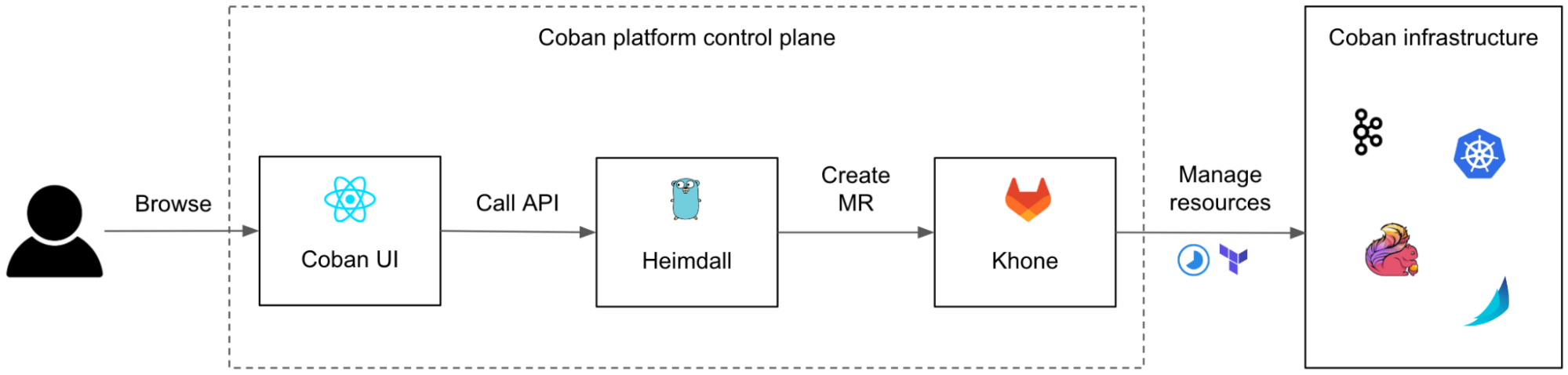
Although we designed the user journey to start from the Coban UI, our users can still opt to communicate with Heimdall and with Khone directly, e.g. for batch changes, or just because many engineers love Git and we want to encourage broad adoption. To make sure that data is eventually consistent across the three systems, we made Khone the only persistent storage layer. Heimdall regularly fetches data from Khone, caches it, and presents it to the Coban UI upon each query.
We also continued using Terraform for all resources, instead of mixing various declarative infrastructure approaches (e.g. Kubernetes Custom Resource Definition, Helm charts), for the sake of consistency of the logic in Khone’s CI pipelines.
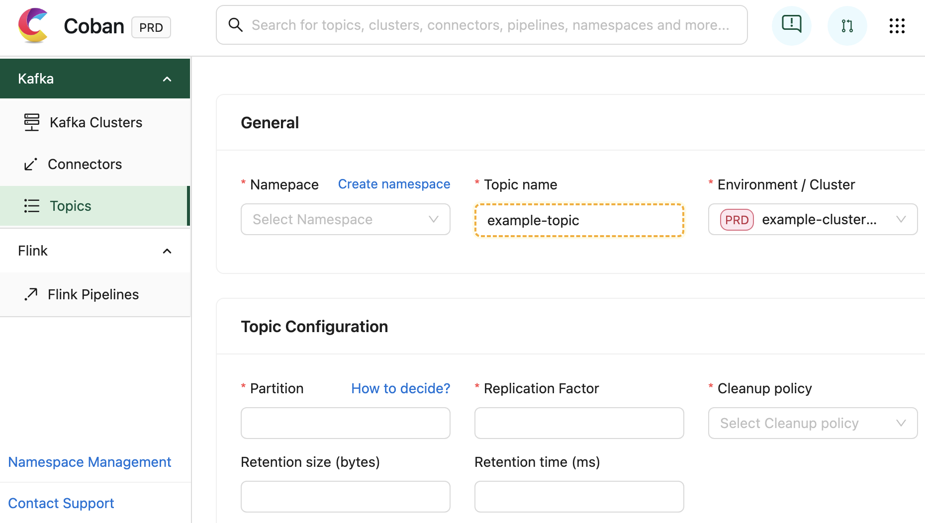
Coban UI
The Coban UI is a React Single Page Application (React SPA) designed by our partner team Chroma, a dedicated team of front-end engineers who thrive on building legendary UIs and reusable components for platform teams at Grab.
It serves as a comprehensive self-service portal, enabling users to effortlessly create data streaming resources by filling out web forms with just a few clicks.
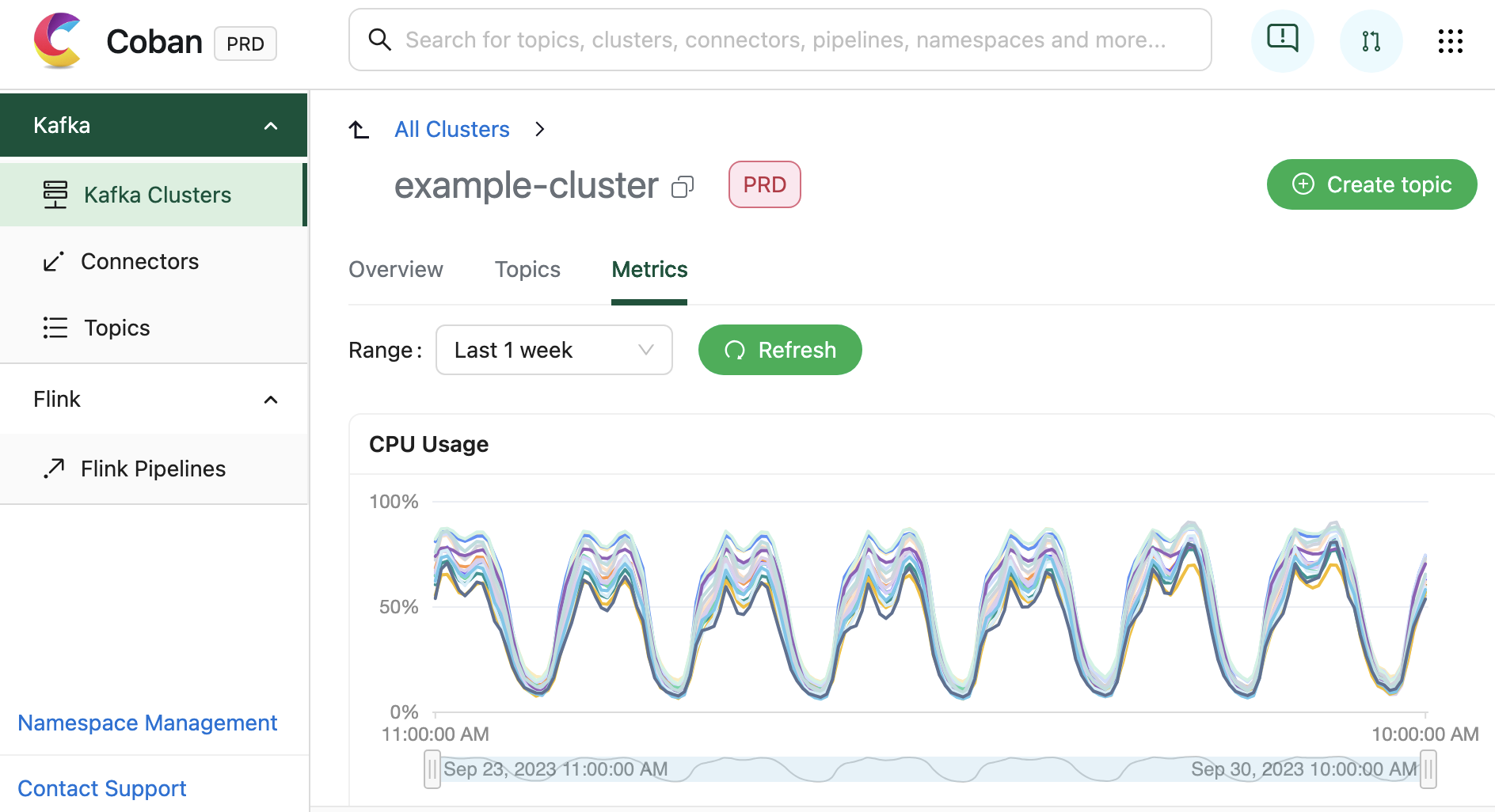
In addition to facilitating resource creation and configuration, the Coban UI is seamlessly integrated with multiple monitoring systems. This integration allows for real-time monitoring of critical metrics and health status for Coban infrastructure components, including Kafka clusters, Kafka topic bytes in/out rates, and more. Under the hood, all this information is exposed by Heimdall APIs.
In terms of infrastructure, the Coban UI is hosted in AWS S3 website hosting. All dynamic content is generated by querying the APIs of the back-end: Heimdall.
Heimdall
Heimdall is the Go back-end of the Coban UI. It serves a collection of APIs for:
- Managing the data streaming resources of the Coban platform with Create, Read, Update and Delete (CRUD) operations, treating the Coban UI as a first-class citizen.
- Exposing the metadata of all Coban resources, so that they can be used by other platforms or searched in the Coban UI.
All operations are authenticated and authorised. Read more about Heimdall’s access control in Migrating from Role to Attribute-based Access Control.
In the next sections, we are going to dive deeper into these two features.
Managing the data streaming resources
First and foremost, Heimdall enables our users to self-manage their data streaming resources. It primarily relies on Khone as its storage and provisioner layer for actual resource management via Git CI pipelines. Therefore, we designed Heimdall’s resource management workflow to leverage the underlying Git flow.
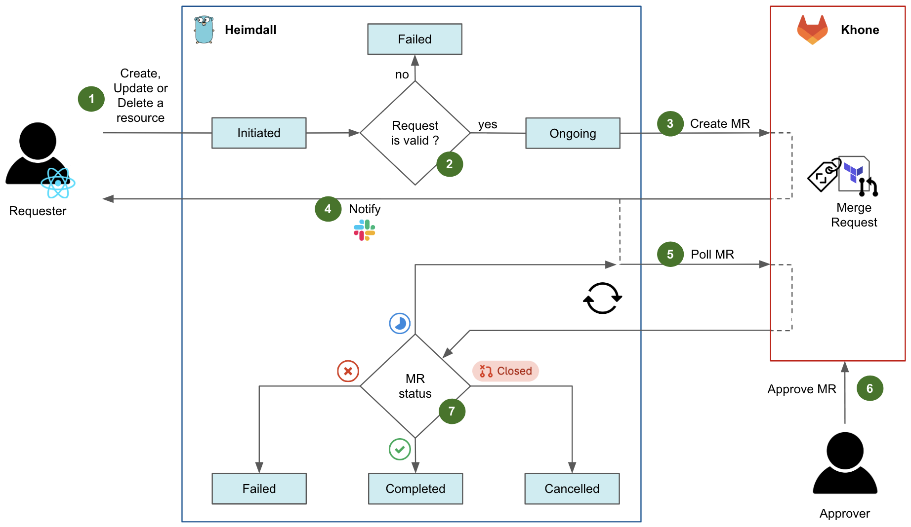
Fig. 4 shows the diagram flow of a typical request in Heimdall to create, update, or delete a resource.
- An authenticated user initiates a request, either by navigating in the Coban UI or by calling the Heimdall API directly. At this stage, the request state is
Initiatedon Heimdall. - Heimdall validates the request against multiple validation rules. For example, if an ongoing change request exists for the same resource, the request fails. If all tests succeed, the request state moves to
Ongoing. - Heimdall then creates an MR in Khone, which contains the Terraform files describing the desired state of the resource, as well as an in-house metadata file describing the key attributes of both resource and requester.
- After the MR has been created successfully, Heimdall notifies the requester via Slack and shares the MR URL.
- After that, Heimdall starts polling the status of the MR in a loop.
- For changes pertaining to production resources, an approver who is code owner in the repository of the resource has to approve the MR. Typically, the approver is an immediate teammate of the requester. Indeed, as a platform team, we empower our users to manage their own resources in a self-service fashion. Ultimately, the requester would merge the MR to trigger the CI pipeline applying the actual Terraform changes. Note that for staging resources, this entire step 6 is automatically performed by Heimdall.
- Depending on the MR status and the status of its CI pipeline in Khone, the final state of the request can be:
Failedif the CI pipeline has failed in Khone.Completedif the CI pipeline has succeeded in Khone.Cancelledif the MR was closed in Khone.
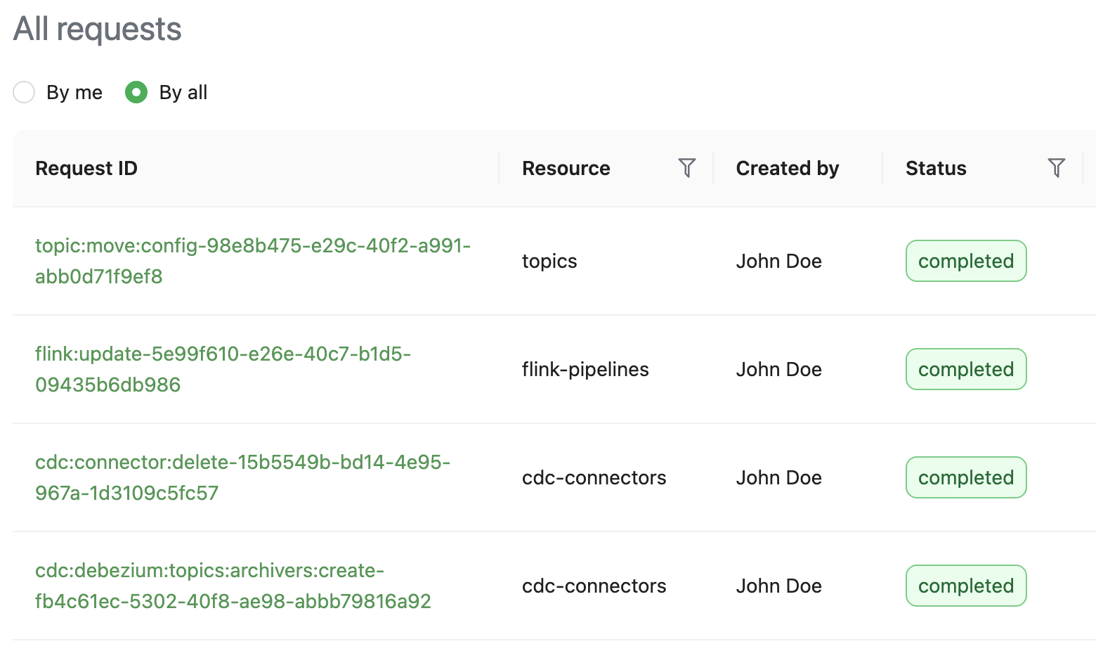
Heimdall exposes APIs to let users track the status of their requests. In the Coban UI, a page queries those APIs to elegantly display the requests.
Exposing the metadata
Apart from managing the data streaming resources, Heimdall also centralises and exposes the metadata pertaining to those resources so other Grab systems can fetch and use it. They can make various queries, for example, listing the producers and consumers of a given Kafka topic, or determining if a database (DB) is the data source for any CDC pipeline.
To make this happen, Heimdall not only retains the metadata of all of the resources that it creates, but also regularly ingests additional information from a variety of upstream systems and platforms, to enrich and make this metadata comprehensive.
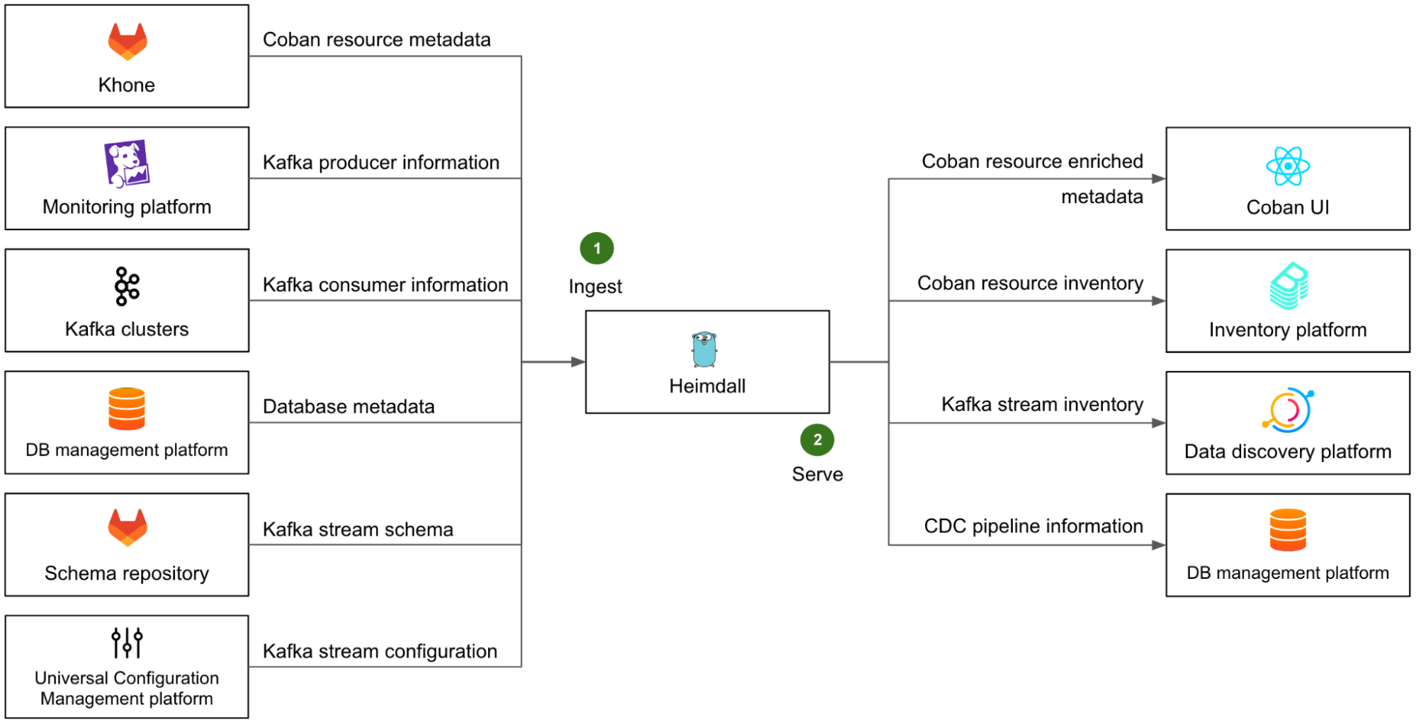
On the left side of Fig. 6, we illustrate Heimdall’s ingestion mechanism with several examples (step 1):
- The metadata of all Coban resources is ingested from Khone. This means the metadata of the resources that were created directly in Khone is also available in Heimdall.
- The list of Kafka producers is retrieved from our monitoring platform, where most of them emit metrics.
- The list of Kafka consumers is retrieved directly from the respective Kafka clusters, by listing the consumer groups and respective Client IDs of each partition.
- The metadata of all DBs, that are used as a data source for CDC pipelines, is fetched from Grab’s internal DB management platform.
- The Kafka stream schemas are retrieved from the Coban schema repository.
- The Kafka stream configuration of each stream is retrieved from Grab Universal Configuration Management platform.
With all of this ingested data, Heimdall can provide comprehensive and accurate information about all data streaming resources to any other Grab platforms via a set of dedicated APIs.
The right side of Fig. 6 shows some examples (step 2) of Heimdall’s serving mechanism:
- As a downstream of Heimdall, the Coban UI enables our direct users to conveniently browse their data streaming resources and access their attributes.
- The entire resource inventory is ingested into the broader Grab inventory platform, based on backstage.io.
- The Kafka streams are ingested into Grab’s internal data discovery platform, based on DataHub, where users can discover and trace the lineage of any piece of data.
- The CDC connectors pertaining to DBs are ingested by Grab internal DB management platform, so that they are made visible in that platform when users are browsing their DBs.
Note that the downstream platforms that ingest data from Heimdall each expose a particular view of the Coban inventory that serves their purpose, but the Coban platform remains the only source of truth for any data streaming resource at Grab.
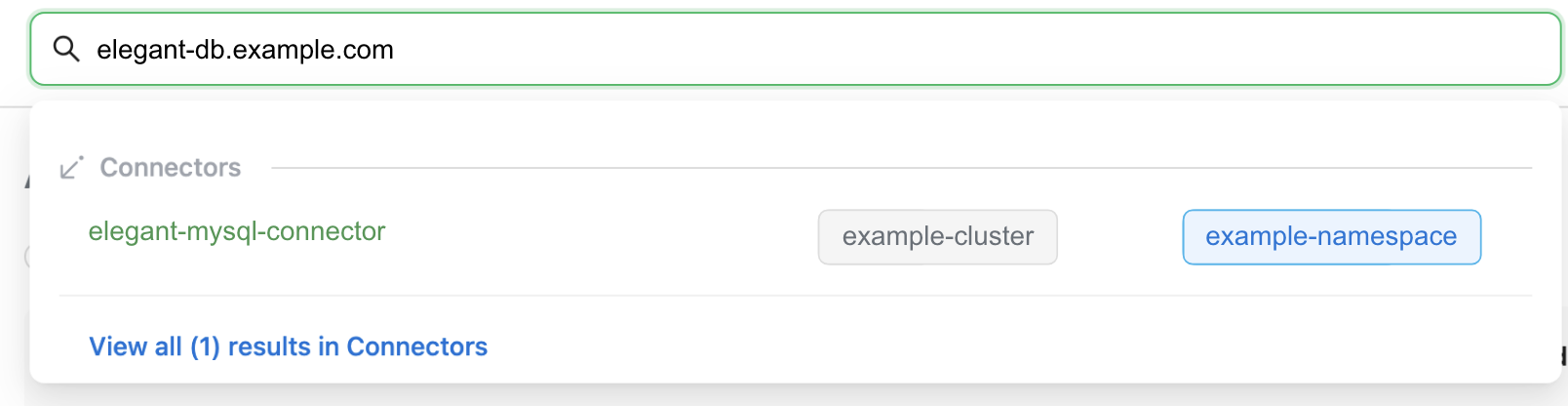
Lastly, Heimdall leverages an internal MySQL DB to support quick data query and exploration. The corresponding API is called by the Coban UI to let our users conveniently search globally among all resources’ attributes.
Khone
Khone is the persistent storage layer of our platform, as well as the executor for actual resource creation, changes, and deletion. Under the hood, it is actually a GitLab repository of Terraform code in typical GitOps fashion, with CI pipelines to plan and apply the Terraform changes automatically. In addition, it also stores a metadata file for each resource.
Compared to letting the platform create the infrastructure directly and keep track of the desired state in its own way, relying on a standard IaC tool like Terraform for the actual changes to the infrastructure presents two major advantages:
- The Terraform code can directly be used for disaster recovery. In case of a disaster, any entitled Cobaner with a local copy of the main branch of the Khone repository is able to recreate all our platform resources directly from their machine. There is no need to rebuild the entire platform’s control plane, thus reducing our Recovery Time Objective (RTO).
- Minimal effort required to follow the API changes of our infrastructure ecosystem (AWS, Kubernetes, Kafka, etc.). When such a change happens, all we need to do is to update the corresponding Terraform provider.
If you’d like to read more about Khone, check out Securing GitOps pipelines. In this section, we will only focus on Khone’s features that are relevant from the platform perspective.
Lightweight Terraform
In Khone, each resource is stored as a Terraform definition. There are two major differences from a normal Terraform project:
- No Terraform environment, such as the required Terraform providers and the location of the remote Terraform state file. They are automatically generated by the CI pipeline via a simple wrapper.
- Only vetted Khone Terraform modules can be used. This is controlled and enforced by the CI pipeline via code inspection. There is one such Terraform module for each kind of supported resource of our platform (e.g. Kafka topic, Flink pipeline, Kafka Connect mirror source connector etc.). Furthermore, those in-house Terraform modules are designed to automatically derive their key variables (e.g. resource name, cluster name, environment) from the relative path of the parent Terraform project in the Khone repository.
Those characteristics are designed to limit the risk and blast radius of human errors. They also make sure that all resources created in Khone are supported by our platform, so that they can also be discovered and managed in Heimdall and the Coban UI. Lastly, by generating the Terraform environment on the fly, we can destroy resources simply by deleting the directory of the project in the code base – this would not be possible otherwise.
Resource metadata
All resource metadata is stored in a YAML file that is present in the Terraform directory of each resource in the Khone repository. This is mainly used for ownership and cost attribution.
With this metadata, we can:
- Better communicate with our users whenever their resources are impacted by an incident or an upcoming maintenance operation.
- Help teams understand the costs of their usage of our platform, a significant step towards cost efficiency.
There are two different ways resource metadata can be created:
- Automatically through Heimdall: The YAML metadata file is automatically generated by Heimdall.
- Through Khone by a human user: The user needs to prepare the YAML metadata file and include it in the MR. This file is then verified by the CI pipeline.
Outcome
The initial version of the three-tier Coban platform, as described in this article, was internally released in March 2022, supporting only Kafka topic management at the time. Since then, we have added support for Flink pipelines, four kinds of Kafka Connect connectors, CDC pipelines, and more recently, Apache Zeppelin notebooks. At the time of writing, the Coban platform manages about 5000 data streaming resources, all described as IaC under the hood.
Our platform also exposes enriched metadata that includes the full data lineage from Kafka producers to Kafka consumers, as well as ownership information, and cost attribution.
With that, our monthly active users have almost quadrupled, truly moving the needle towards democratising the usage of real-time data within all Grab verticals.
In spite of that user growth, the end-to-end workflow success rate for self-served resource creation, change or deletion, remained well above 90% in the first half of 2023, while the Heimdall API uptime was above 99.95%.
Challenges faced
A common challenge for platform teams resides in the misalignment between the Service Level Objective (SLO) of the platform, and the various environments (e.g. staging, production) of the managed resources and upstream/downstream systems and platforms.
Indeed, the platform aims to guarantee the same level of service, regardless of whether it is used to create resources in the staging or the production environment. From the platform team’s perspective, the platform as a whole is considered production-grade, as soon as it serves actual users.
A naive approach to address this challenge is to let the production version of the platform manage all resources regardless of their respective environments. However, doing so does not permit a hermetic segregation of the staging and production environments across the organisation, which is a good security practice, and often a requirement for compliance. For example, the production version of the platform would have to connect to upstream systems in the staging environment, e.g. staging Kafka clusters to collect their consumer groups, in the case of Heimdall. Conversely, the staging version of certain downstreams would have to connect to the production version of Heimdall, to fetch the metadata of relevant staging resources.
The alternative approach, generally adopted across Grab, is to instantiate all platforms in each environment (staging and production), while still considering both instances as production-grade and guaranteeing tight SLOs in both environments.
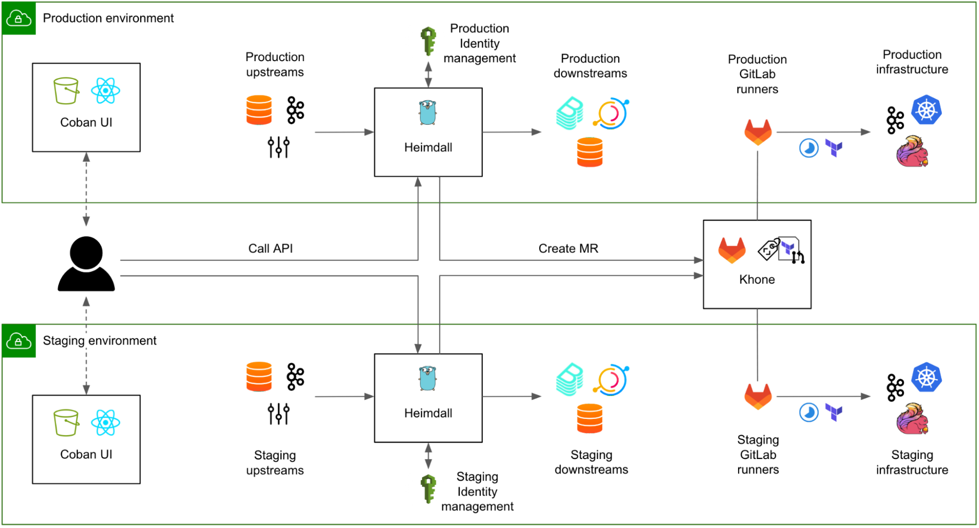
In Fig. 8, both instances of Heimdall have equivalent SLOs. The caveat is that all upstream systems and platforms must also guarantee a strict SLO in both environments. This obviously comes with a cost, for example, tighter maintenance windows for the operations pertaining to the Kafka clusters in the staging environment.
A strong “platform” culture is required for platform teams to fully understand that their instance residing in the staging environment is not their own staging environment and should not be used for testing new features.
What’s next?
Currently, users creating, updating, or deleting production resources in the Coban UI (or directly by calling Heimdall API) receive the URL of the generated GitLab MR in a Slack message. From there, they must get the MR approved by a code owner, typically another team member, and finally merge the MR, for the requested change to be actually implemented by the CI pipeline.
Although this was a fairly easy way to implement a maker/checker process that was immediately compliant with our regulatory requirements for any changes in production, the user experience is not optimal. In the near future, we plan to bring the approval mechanism into Heimdall and the Coban UI, while still providing our more advanced users with the option to directly create, approve, and merge MRs in GitLab. In the longer run, we would also like to enhance the Coban UI with the output of the Khone CI jobs that include the Terraform plan and apply results.
There is another aspect of the platform that we want to improve. As Heimdall regularly polls the upstream platforms to collect their metadata, this introduces a latency between a change in one of those platforms and its reflection in the Coban platform, which can hinder the user experience. To refresh resource metadata in Heimdall in near real time, we plan to leverage an existing Grab-wide event stream, where most of the configuration and code changes at Grab are produced as events. Heimdall will soon be able to consume those events and update the metadata of the affected resources immediately, without waiting for the next periodic refresh.
Join us
Grab is the leading superapp platform in Southeast Asia, providing everyday services that matter to consumers. More than just a ride-hailing and food delivery app, Grab offers a wide range of on-demand services in the region, including mobility, food, package and grocery delivery services, mobile payments, and financial services across 428 cities in eight countries.
Powered by technology and driven by heart, our mission is to drive Southeast Asia forward by creating economic empowerment for everyone. If this mission speaks to you, join our team today!
Fall 2023 SOC reports now available with 171 services in scope
Post Syndicated from Ryan Wilks original https://aws.amazon.com/blogs/security/fall-2023-soc-reports-now-available-with-171-services-in-scope/
At Amazon Web Services (AWS), we’re committed to providing our customers with continued assurance over the security, availability, confidentiality, and privacy of the AWS control environment.
We’re proud to deliver the Fall 2023 System and Organizational (SOC) 1, 2, and 3 reports to support your confidence in AWS services. The reports cover the period October 1, 2022, to September 30, 2023. We extended the period of coverage to 12 months so that you have a full year of assurance from a single report. We also updated the associated infrastructure supporting our in-scope products and services to reflect new edge locations, AWS Wavelength zones, and AWS Local Zones.
The SOC 2 report includes the Security, Availability, Confidentiality, and Privacy Trust Service Criteria that cover both the design and operating effectiveness of controls over a period of time. The SOC 2 Privacy Trust Service Criteria, developed by the American Institute of Certified Public Accountants (AICPA), establishes the criteria for evaluating controls and how personal information is collected, used, retained, disclosed, and disposed of. For more information about our privacy commitments supporting the SOC 2 Type 2 report, see the AWS Customer Agreement.
The scope of the Fall 2023 SOC 2 Type 2 report includes information about how we handle the content that you upload to AWS, and how we protect that content across the services and locations that are in scope for the latest AWS SOC reports.
The Fall 2023 SOC reports include an additional 13 services in scope, for a total of 171 services. See the full list on our Services in Scope by Compliance Program page.
Here are the 13 additional services in scope for the Fall 2023 SOC reports:
- AWS AppFabric
- AWS Artifact
- Amazon Bedrock
- AWS Clean Rooms
- AWS Fault Injection Simulator
- AWS HealthImaging
- AWS HealthOmics
- Amazon Inspector
- AWS IoT Device Defender
- AWS IoT TwinMaker
- AWS Resilience Hub
- AWS User Notifications
- AWS Wickr
Customers can download the Fall 2023 SOC reports through AWS Artifact in the AWS Management Console. You can also download the SOC 3 report as a PDF file from AWS.
AWS strives to bring services into the scope of its compliance programs to help you meet your architectural and regulatory needs. If there are additional AWS services that you would like us to add to the scope of our SOC reports (or other compliance programs), reach out to your AWS representatives.
We value your feedback and questions. Feel free to reach out to the team through the Contact Us page. If you have feedback about this post, submit comments in the Comments section below.
Want more AWS Security how-to-content, news, and feature announcements? Follow us on Twitter.
LibreQoS 1.4 released
Post Syndicated from corbet original https://lwn.net/Articles/953286/
The LibreQoS project
describes itself as:
LibreQoS is a Quality of Experience (QoE) Smart Queue Management
(SQM) system designed for Internet Service Providers to optimize
the flow of their network traffic and thus reduce bufferbloat, keep
the network responsive, and improve the end-user experience.
Version
1.4 of LibreQoS was released on November 17. “Version 1.4 is a
”
huge milestone. A whole new back-end, new GUI, 30%+ performance
improvements, support for single-interface mode.
[$] An overview of kernel samepage merging (KSM)
Post Syndicated from jake original https://lwn.net/Articles/953141/
In the Kernel Summit
track at the 2023 Linux
Plumbers Conference (LPC), Stefan Roesch led a session on kernel
samepage merging (KSM). He gave an overview of the feature and described
some recent changes to KSM. He showed how
an application can enable KSM to deduplicate its memory and how the feature
can be evaluated to determine whether it is a good fit for new workloads.
In addition, he provided some real-world data of the benefits from his
workplace at Meta.
All of Netflix’s HDR video streaming is now dynamically optimized
Post Syndicated from Netflix Technology Blog original https://netflixtechblog.com/all-of-netflixs-hdr-video-streaming-is-now-dynamically-optimized-e9e0cb15f2ba
by Aditya Mavlankar, Zhi Li, Lukáš Krasula and Christos Bampis
High dynamic range (HDR) video brings a wider range of luminance and a wider gamut of colors, paving the way for a stunning viewing experience. Separately, our invention of Dynamically Optimized (DO) encoding helps achieve optimized bitrate-quality tradeoffs depending on the complexity of the content.
HDR was launched at Netflix in 2016 and the number of titles available in HDR has been growing ever since. We were, however, missing the systematic ability to measure perceptual quality (VMAF) of HDR streams since VMAF was limited to standard dynamic range (SDR) video signals.
As noted in an earlier blog post, we began developing an HDR variant of VMAF; let’s call it HDR-VMAF. A vital aspect of such development is subjective testing with HDR encodes in order to generate training data. The pandemic, however, posed unique challenges in conducting a conventional in-lab subjective test with HDR encodes. We improvised as part of a collaborative effort with Dolby Laboratories and conducted subjective tests with 4K-HDR content using high-end OLED panels in calibrated conditions created in participants’ homes [1],[2]. Details pertaining to HDR-VMAF exceed the scope of this article and will be covered in a future blog post; for now, suffice it to say that the first version of HDR-VMAF landed internally in 2021 and we have been improving the metric ever since.
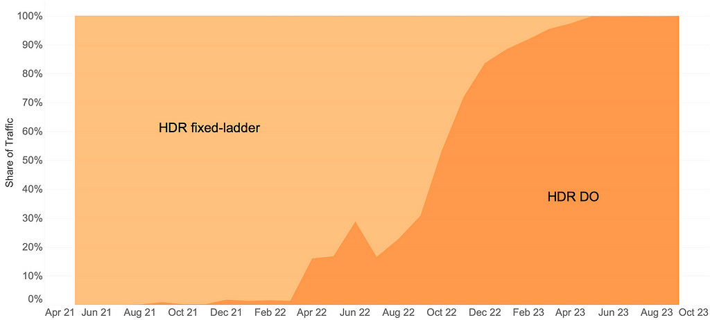
The arrival of HDR-VMAF allowed us to create HDR streams with DO applied, i.e., HDR-DO encodes. Prior to that, we were using a fixed ladder with predetermined bitrates — regardless of content characteristics — for HDR video streaming. We A/B tested HDR-DO encodes in production in Q3-Q4 2021, followed by improving the ladder generation algorithm further in early 2022. We started backfilling HDR-DO encodes for existing titles from Q2 2022. By June 2023 the entire HDR catalog was optimized. The graphic below (Fig. 1) depicts the migration of traffic from fixed bitrates to DO encodes.
Bitrate versus quality comparison
HDR-VMAF is designed to be format-agnostic — it measures the perceptual quality of HDR video signal regardless of its container format, for example, Dolby Vision or HDR10. HDR-VMAF focuses on the signal characteristics (as a result of lossy encoding) instead of display characteristics, and thus it does not include display mapping in its pipeline. Display mapping is the specific tone mapping applied by the display based on its own characteristics — peak luminance, black level, color gamut, etc. — and based on content characteristics and/or metadata signaled in the bitstream.
Two ways that HDR10 and Dolby Vision differ are: 1) the preprocessing applied to the signal before encoding 2) the metadata informing the display mapping on different displays. So, HDR-VMAF will capture the effect of 1) but ignore the effect of 2). Display capabilities vary a lot among the heterogeneous population of devices that stream HDR content — this aspect is similar to other factors that vary session to session such as ambient lighting, viewing distance, upscaling algorithm on the device, etc. “VMAF not incorporating display mapping” implies the scores are computed for an “ideal display” that’s capable of representing the entire luminance range and the entire color gamut spanned by the video signal — thus not requiring display mapping. This background is useful to have before looking at rate vs quality curves pertaining to these two formats.
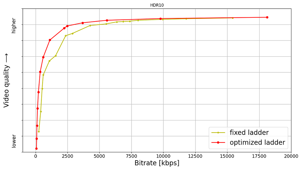
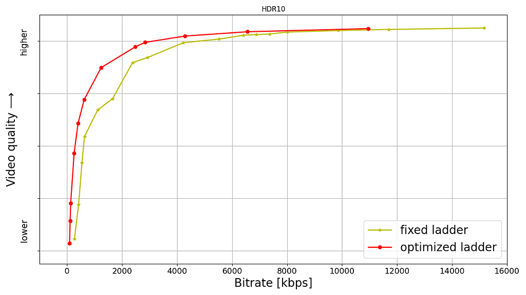
Shown below are rate versus quality examples for a couple of titles from our HDR catalog. We present two sets. Within each set we show curves for both Dolby Vision and HDR10. The first set (Fig. 2) corresponds to an episode from a gourmet cooking show incorporating fast-paced scenes from around the world. The second set (Fig. 3) corresponds to an episode from a relatively slower drama series; slower in terms of camera action. The optimized encodes are chosen from the convex hull formed by various rate-quality points corresponding to different bitrates, spatial resolutions and encoding recipes.
For brevity we skipped annotating ladder points with their spatial resolutions but the overall observations from our previous article on SDR-4K encode optimization apply here as well. The fixed ladder is slow in ramping up spatial resolution, so the quality stays almost flat among two successive 1080p points or two successive 4K points. On the other hand, the optimized ladder presents a sharper increase in quality with increasing bitrate.
The fixed ladder has predetermined 4K bitrates — 8, 10, 12 and 16 Mbps — it deterministically maxes out at 16 Mbps. On the other hand, the optimized ladder targets very high levels of quality on the top rung of the bitrate ladder, even at the cost of higher bitrates if the content is complex, thereby satisfying the most discerning viewers. In spite of reaching higher qualities than the fixed ladder, the HDR-DO ladder, on average, occupies only 58% of the storage space compared to fixed-bitrate ladder. This is achieved by more efficiently spacing the ladder points, especially in the high-bitrate region. After all, there is little to no benefit in packing multiple high-bitrate points so close to each other — for example, 3 QHD (2560×1440) points placed in the 6 to 7.5 Mbps range followed by the four 4K points at 8, 10, 12 and 16 Mbps, as was done on the fixed ladder.


It is important to note that the fixed-ladder encodes had constant duration group-of-pictures (GoPs) and suffered from some inefficiency due to shot boundaries not aligning with Instantaneous Decoder Refresh (IDR) frames. The DO encodes are shot-based and so the IDR frames align with shot boundaries. For a given rate-quality operating point, the DO process helps allocate bits among the various shots while maximizing an overall objective function. Also thanks to the DO framework, within a given rate-quality operating point, challenging shots can and do burst in bitrate up to the codec level limit associated with that point.
Member benefits
We A/B tested the fixed and optimized ladders; first and foremost to make sure that devices in the field can handle the new streams and serving new streams doesn’t cause unintended playback issues. A/B testing also allows us to get a read on the improvement in quality of experience (QoE). Overall, the improvements can be summarized as:
- 40% fewer rebuffers
- Higher video quality for both bandwidth-constrained as well as unconstrained sessions
- Lower initial bitrate
- Higher initial quality
- Lower play delay
- Less variation in delivered video quality
- Lower Internet data usage, especially on mobiles and tablets
Will HDR-VMAF be open-source?
Yes, we are committed to supporting the open-source community. The current implementation, however, is largely tailored to our internal pipelines. We are working to ensure it is versatile, stable, and easy-to-use for the community. Additionally, the current version has some algorithmic limitations that we are in the process of improving before the official release. When we do release it, HDR-VMAF will have higher accuracy in perceptual quality prediction, and be easier to use “out of the box”.
Summary
Thanks to the arrival of HDR-VMAF, we were able to optimize our HDR encodes. Fixed-ladder HDR encodes have been fully replaced by optimized ones, reducing storage footprint and Internet data usage — and most importantly, improving the video quality for our members. Improvements have been seen across all device categories ranging from TVs to mobiles and tablets.
Acknowledgments
We thank all the volunteers who participated in the subjective experiments. We also want to acknowledge the contributions of our colleagues from Dolby, namely Anustup Kumar Choudhury, Scott Daly, Robin Atkins, Ludovic Malfait, and Suzanne Farrell, who helped with preparations and conducting of the subjective tests.
We thank Matthew Donato, Adithya Prakash, Rich Gerber, Joe Drago, Benbuck Nason and Joseph McCormick for all the interesting discussions on HDR video.
We thank various internal teams at Netflix for the crucial roles they play:
- The various client device and UI engineering teams at Netflix that manage the Netflix experience on various device platforms
- The data science and engineering teams at Netflix that help us run and analyze A/B tests; we thank Chris Pham in particular for generating various data insights for the encoding team
- The Playback Systems team that steers the Netflix experience for every client device including the experience served in various encoding A/B tests
- The Open Connect team that manages Netflix’s own content delivery network
- The Content Infrastructure and Solutions team that manages the compute platform that enables us to execute video encoding at scale
- The Streaming Encoding Pipeline team that helps us orchestrate the generation of various streaming assets
Find our work interesting? Join us and be a part of the amazing team that brought you this tech-blog; open positions:
References
[1] L. Krasula, A. Choudhury, S. Daly, Z. Li, R. Atkins, L. Malfait, A. Mavlankar, “Subjective video quality for 4K HDR-WCG content using a browser-based approach for “at-home” testing,” Electronic Imaging, vol. 35, pp. 263–1–8 (2023) [online]
[2] A. Choudhury, L. Krasula, S. Daly, Z. Li, R. Atkins, L. Malfait, “Testing 4K HDR-WCG professional video content for subjective quality using a remote testing approach,” SMPTE Media Technology Summit 2023
![]()
All of Netflix’s HDR video streaming is now dynamically optimized was originally published in Netflix TechBlog on Medium, where people are continuing the conversation by highlighting and responding to this story.
Optimize AWS administration with IAM paths
Post Syndicated from David Rowe original https://aws.amazon.com/blogs/security/optimize-aws-administration-with-iam-paths/
As organizations expand their Amazon Web Services (AWS) environment and migrate workloads to the cloud, they find themselves dealing with many AWS Identity and Access Management (IAM) roles and policies. These roles and policies multiply because IAM fills a crucial role in securing and controlling access to AWS resources. Imagine you have a team creating an application. You create an IAM role to grant them access to the necessary AWS resources, such as Amazon Simple Storage Service (Amazon S3) buckets, Amazon Key Management Service (Amazon KMS) keys, and Amazon Elastic File Service (Amazon EFS) shares. With additional workloads and new data access patterns, the number of IAM roles and policies naturally increases. With the growing complexity of resources and data access patterns, it becomes crucial to streamline access and simplify the management of IAM policies and roles
In this blog post, we illustrate how you can use IAM paths to organize IAM policies and roles and provide examples you can use as a foundation for your own use cases.
How to use paths with your IAM roles and policies
When you create a role or policy, you create it with a default path. In IAM, the default path for resources is “/”. Instead of using a default path, you can create and use paths and nested paths as a structure to manage IAM resources. The following example shows an IAM role named S3Access in the path developer:
Service-linked roles are created in a reserved path /aws-service-role/. The following is an example of a service-linked role path.
The following example is of an IAM policy named S3ReadOnlyAccess in the path security:
Why use IAM paths with roles and policies?
By using IAM paths with roles and policies, you can create groupings and design a logical separation to simplify management. You can use these groupings to grant access to teams, delegate permissions, and control what roles can be passed to AWS services. In the following sections, we illustrate how to use IAM paths to create groupings of roles and policies by referencing a fictional company and its expansion of AWS resources.
First, to create roles and policies with a path, you use the IAM API or AWS Command Line Interface (AWS CLI) to run aws cli create-role.
The following is an example of an AWS CLI command that creates a role in an IAM path.
Replace <ROLE-NAME> and <PATH> in the command with your role name and role path respectively. Use a trust policy for the trust document that matches your use case. An example trust policy that allows Amazon Elastic Compute Cloud (Amazon EC2) instances to assume this role on your behalf is below:
The following is an example of an AWS CLI command that creates a policy in an IAM path.
IAM paths sample implementation
Let’s assume you’re a cloud platform architect at AnyCompany, a startup that’s planning to expand its AWS environment. By the end of the year, AnyCompany is going to expand from one team of developers to multiple teams, all of which require access to AWS. You want to design a scalable way to manage IAM roles and policies to simplify the administrative process to give permissions to each team’s roles. To do that, you create groupings of roles and policies based on teams.
Organize IAM roles with paths
AnyCompany decided to create the following roles based on teams.
| Team name | Role name | IAM path | Has access to |
| Security | universal-security-readonly | /security/ | All resources |
| Team A database administrators | DBA-role-A | /teamA/ | TeamA’s databases |
| Team B database administrators | DBA-role-B | /teamB/ | TeamB’s databases |
The following are example Amazon Resource Names (ARNs) for the roles listed above. In this example, you define IAM paths to create a grouping based on team names.
- arn:aws:iam::444455556666:role/security/universal-security-readonly-role
- arn:aws:iam::444455556666:role/teamA/DBA-role-A
- arn:aws:iam::444455556666:role/teamB/DBA-role-B
Note: Role names must be unique within your AWS account regardless of their IAM paths. You cannot have two roles named DBA-role, even if they’re in separate paths.
Organize IAM policies with paths
After you’ve created roles in IAM paths, you will create policies to provide permissions to these roles. The same path structure that was defined in the IAM roles is used for the IAM policies. The following is an example of how to create a policy with an IAM path. After you create the policy, you can attach the policy to a role using the attach-role-policy command.
- arn:aws:iam::444455556666:policy/security/universal-security-readonly-policy
- arn:aws:iam::444455556666:policy/teamA/DBA-policy-A
- arn:aws:iam::444455556666:policy/teamB/DBA-policy-B
Grant access to groupings of IAM roles with resource-based policies
Now that you’ve created roles and policies in paths, you can more readily define which groups of principals can access a resource. In this deny statement example, you allow only the roles in the IAM path /teamA/ to act on your bucket, and you deny access to all other IAM principals. Rather than use individual roles to deny access to the bucket, which would require you to list every role, you can deny access to an entire group of principals by path. If you create a new role in your AWS account in the specified path, you don’t need to modify the policy to include them. The path-based deny statement will apply automatically.
Delegate access with IAM paths
IAM paths can also enable teams to more safely create IAM roles and policies and allow teams to only use the roles and policies contained by the paths. Paths can help prevent teams from privilege escalation by denying the use of roles that don’t belong to their team.
Continuing the example above, AnyCompany established a process that allows each team to create their own IAM roles and policies, providing they’re in a specified IAM path. For example, AnyCompany allows team A to create IAM roles and policies for team A in the path /teamA/:
- arn:aws:iam::444455556666:role/teamA/<role-name>
- arn:aws:iam::444455556666:policy/teamA/<policy-name>
Using IAM paths, AnyCompany can allow team A to more safely create and manage their own IAM roles and policies and safely pass those roles to AWS services using the iam:PassRole permission.
At AnyCompany, four IAM policies using IAM paths allow teams to more safely create and manage their own IAM roles and policies. Following recommended best practices, AnyCompany uses infrastructure as code (IaC) for all IAM role and policy creation. The four path-based policies that follow will be attached to each team’s CI/CD pipeline role, which has permissions to create roles. The following example focuses on team A, and how these policies enable them to self-manage their IAM credentials.
- Create a role in the path and modify inline policies on the role: This policy allows three actions: iam:CreateRole, iam:PutRolePolicy, and iam:DeleteRolePolicy. When this policy is attached to a principal, that principal is allowed to create roles in the IAM path /teamA/ and add and delete inline policies on roles in that IAM path.
- Add and remove managed policies: The second policy example allows two actions: iam:AttachRolePolicy and iam:DetachRolePolicy. This policy allows a principal to attach and detach managed policies in the /teamA/ path to roles that are created in the /teamA/ path.
- Delete roles, tag and untag roles, read roles: The third policy allows a principal to delete roles, tag and untag roles, and retrieve information about roles that are created in the /teamA/ path.
- Policy management in IAM path: The final policy example allows access to create, modify, get, and delete policies that are created in the /teamA/ path. This includes creating, deleting, and tagging policies.
Safely pass roles with IAM paths and iam:PassRole
To pass a role to an AWS service, a principal must have the iam:PassRole permission. IAM paths are the recommended option to restrict which roles a principal can pass when granted the iam:PassRole permission. IAM paths help verify principals can only pass specific roles or groupings of roles to an AWS service.
At AnyCompany, the security team wants to allow team A to add IAM roles to an instance profile and attach it to Amazon EC2 instances, but only if the roles are in the /teamA/ path. The IAM action that allows team A to provide the role to the instance is iam:PassRole. The security team doesn’t want team A to be able to pass other roles in the account, such as an administrator role.
The policy that follows allows passing of a role that was created in the /teamA/ path and does not allow the passing of other roles such as an administrator role.
How to create preventative guardrails for sensitive IAM paths
You can use service control policies (SCP) to restrict access to sensitive roles and policies within specific IAM paths. You can use an SCP to prevent the modification of sensitive roles and policies that are created in a defined path.
You will see the IAM path under the resource and condition portion of the statement. Only the role named IAMAdministrator created in the /security/ path can create or modify roles in the security path. This SCP allows you to delegate IAM role and policy management to developers with confidence that they won’t be able to create, modify, or delete any roles or policies in the security path.
This next example shows you how you can safely exempt IAM roles created in the security path from specific controls in your organization. The policy denies all roles except the roles created in the /security/ IAM path to close member accounts.
Additional considerations when using IAM paths
You should be aware of some additional considerations when you start using IAM paths.
- Paths are immutable for IAM roles and policies. To change a path, you must delete the IAM resource and recreate the IAM resource in the alternative path. Deleting roles or instance profiles has step-by-step instructions to delete an IAM resource.
- You can only create IAM paths using AWS API or command line tools. You cannot create IAM paths with the AWS console.
- IAM paths aren’t added to the uniqueness of the role name. Role names must be unique within your account without the path taken into consideration.
- AWS reserves several paths including /aws-service-role/ and you cannot create roles in this path.
Conclusion
IAM paths provide a powerful mechanism for effectively grouping IAM resources. Path-based groupings can streamline access management across AWS services. In this post, you learned how to use paths with IAM principals to create structured access with IAM roles, how to delegate and segregate access within an account, and safely pass roles using iam:PassRole. These techniques can empower you to fine-tune your AWS access management and help improve security while streamlining operational workflows.
You can use the following references to help extend your knowledge of IAM paths. This post references the processes outlined in the user guides and blog post, and sources the IAM policies from the GitHub repositories.
- AWS Organizations User Guide, SCP General Examples
- AWS-Samples Service-control-policy-examples GitHub Repository
- AWS Security Blog: IAM Policy types: How and when to use them
- AWS-Samples how-and-when-to-use-aws-iam-policy-blog-samples GitHub Repository
If you have feedback about this post, submit comments in the Comments section below. If you have questions about this post, contact AWS Support.
Want more AWS Security news? Follow us on Twitter.
Build and manage your modern data stack using dbt and AWS Glue through dbt-glue, the new “trusted” dbt adapter
Post Syndicated from Noritaka Sekiyama original https://aws.amazon.com/blogs/big-data/build-and-manage-your-modern-data-stack-using-dbt-and-aws-glue-through-dbt-glue-the-new-trusted-dbt-adapter/
dbt is an open source, SQL-first templating engine that allows you to write repeatable and extensible data transforms in Python and SQL. dbt focuses on the transform layer of extract, load, transform (ELT) or extract, transform, load (ETL) processes across data warehouses and databases through specific engine adapters to achieve extract and load functionality. It enables data engineers, data scientists, and analytics engineers to define the business logic with SQL select statements and eliminates the need to write boilerplate data manipulation language (DML) and data definition language (DDL) expressions. dbt lets data engineers quickly and collaboratively deploy analytics code following software engineering best practices like modularity, portability, continuous integration and continuous delivery (CI/CD), and documentation.
dbt is predominantly used by data warehouses (such as Amazon Redshift) customers who are looking to keep their data transform logic separate from storage and engine. We have seen a strong customer demand to expand its scope to cloud-based data lakes because data lakes are increasingly the enterprise solution for large-scale data initiatives due to their power and capabilities.
In 2022, AWS published a dbt adapter called dbt-glue—the open source, battle-tested dbt AWS Glue adapter that allows data engineers to use dbt for cloud-based data lakes along with data warehouses and databases, paying for just the compute they need. The dbt-glue adapter democratized access for dbt users to data lakes, and enabled many users to effortlessly run their transformation workloads on the cloud with the serverless data integration capability of AWS Glue. From the launch of the adapter, AWS has continued investing into dbt-glue to cover more requirements.
Today, we are pleased to announce that the dbt-glue adapter is now a trusted adapter based on our strategic collaboration with dbt Labs. Trusted adapters are adapters not maintained by dbt Labs, but adaptors that that dbt Lab is comfortable recommending to users for use in production.
The key capabilities of the dbt-glue adapter are as follows:
- Runs SQL as Spark SQL on AWS Glue interactive sessions
- Manages table definitions on the AWS Glue Data Catalog
- Supports open table formats such as Apache Hudi, Delta Lake, and Apache Iceberg
- Supports AWS Lake Formation permissions for fine-grained access control
In addition to those capabilities, the dbt-glue adapter is designed to optimize resource utilization with several techniques on top of AWS Glue interactive sessions.
This post demonstrates how the dbt-glue adapter helps your workload, and how you can build a modern data stack using dbt and AWS Glue using the dbt-glue adapter.
Common use cases
One common use case for using dbt-glue is if a central analytics team at a large corporation is responsible for monitoring operational efficiency. They ingest application logs into raw Parquet tables in an Amazon Simple Storage Service (Amazon S3) data lake. Additionally, they extract organized data from operational systems capturing the company’s organizational structure and costs of diverse operational components that they stored in the raw zone using Iceberg tables to maintain the original schema, facilitating easy access to the data. The team uses dbt-glue to build a transformed gold model optimized for business intelligence (BI). The gold model joins the technical logs with billing data and organizes the metrics per business unit. The gold model uses Iceberg’s ability to support data warehouse-style modeling needed for performant BI analytics in a data lake. The combination of Iceberg and dbt-glue allows the team to efficiently build a data model that’s ready to be consumed.
Another common use case is when an analytics team in a company that has an S3 data lake creates a new data product in order to enrich its existing data from its data lake with medical data. Let’s say that this company is located in Europe and the data product must comply with the GDPR. For this, the company uses Iceberg to meet needs such as the right to be forgotten and the deletion of data. The company uses dbt to model its data product on its existing data lake due to its compatibility with AWS Glue and Iceberg and the simplicity that the dbt-glue adapter brings to the use of this storage format.
How dbt and dbt-glue work
The following are key dbt features:
- Project – A dbt project enforces a top-level structure on the staging, models, permissions, and adapters. A project can be checked into a GitHub repo for version control.
- SQL – dbt relies on SQL select statements for defining data transformation logic. Instead of raw SQL, dbt offers templatized SQL (using Jinja) that allows code modularity. Instead of having to copy/paste SQL in multiple places, data engineers can define modular transforms and call those from other places within the project. Having a modular pipeline helps data engineers collaborate on the same project.
- Models – dbt models are primarily written as a SELECT statement and saved as a .sql file. Data engineers define dbt models for their data representations. To learn more, refer to About dbt models.
- Materializations – Materializations are strategies for persisting dbt models in a warehouse. There are five types of materializations built into dbt: table, view, incremental, ephemeral, and materialized view. To learn more, refer to Materializations and Incremental models.
- Data lineage – dbt tracks data lineage, allowing you to understand the origin of data and how it flows through different transformations. dbt also supports impact analysis, which helps identify the downstream effects of changes.
The high-level data flow is as follows:
- Data engineers ingest data from data sources to raw tables and define table definitions for the raw tables.
- Data engineers write dbt models with templatized SQL.
- The dbt adapter converts dbt models to SQL statements compatible in a data warehouse.
- The data warehouse runs the SQL statements to create intermediate tables or final tables, views, or materialized views.
The following diagram illustrates the architecture.

dbt-glue works with the following steps:
- The dbt-glue adapter converts dbt models to SQL statements compatible in Spark SQL.
- AWS Glue interactive sessions run the SQL statements to create intermediate tables or final tables, views, or materialized views.
- dbt-glue supports
csv,parquet,hudi,delta, andicebergasfileformat. - On the dbt-glue adapter, table or incremental are commonly used for materializations at the destination. There are three strategies for incremental materialization. The merge strategy requires
hudi,delta, oriceberg. With the other two strategies,appendandinsert_overwrite, you can usecsv,parquet,hudi,delta, oriceberg.
The following diagram illustrates this architecture.

Example use case
In this post, we use the data from the New York City Taxi Records dataset. This dataset is available in the Registry of Open Data on AWS (RODA), which is a repository containing public datasets from AWS resources. The raw Parquet table records in this dataset stores trip records.
The objective is to create the following three tables, which contain metrics based on the raw table:
- silver_avg_metrics – Basic metrics based on NYC Taxi Open Data for the year 2016
- gold_passengers_metrics – Metrics per passenger based on the silver metrics table
- gold_cost_metrics – Metrics per cost based on the silver metrics table
The final goal is to create two well-designed gold tables that store already aggregated results in Iceberg format for ad hoc queries through Amazon Athena.
Prerequisites
The instruction requires following prerequisites:
- An AWS Identity and Access Management (IAM) role with all the mandatory permissions to run an AWS Glue interactive session and the dbt-glue adapter
- An AWS Glue database and table to store the metadata related to the NYC taxi records dataset
- An S3 bucket to use as output and store the processed data
- An Athena configuration (a workgroup and S3 bucket to store the output) to explore the dataset
- An AWS Lambda function (created as an AWS CloudFormation custom resource) that updates all the partitions in the AWS Glue table
With these prerequisites, we simulate the situation that data engineers have already ingested data from data sources to raw tables, and defined table definitions for the raw tables.
For ease of use, we prepared a CloudFormation template. This template deploys all the required infrastructure. To create these resources, choose Launch Stack in the us-east-1 Region, and follow the instructions:
![]()
Install dbt, the dbt CLI, and the dbt adaptor
The dbt CLI is a command line interface for running dbt projects. It’s free to use and available as an open source project. Install dbt and the dbt CLI with the following code:
For more information, refer to How to install dbt, What is dbt?, and Viewpoint.
Install the dbt adapter with the following code:
Create a dbt project
Complete the following steps to create a dbt project:
- Run the
dbt initcommand to create and initialize a new empty dbt project: - For the project name, enter
dbt_glue_demo. - For the database, choose
glue.
Now the empty project has been created. The directory structure is shown as follows:
Create a source
The next step is to create a source table definition. We add models/source_tables.yml with the following contents:
This source definition corresponds to the AWS Glue table nyctaxi.records, which we created in the CloudFormation stack.
Create models
In this step, we create a dbt model that represents the average values for trip duration, passenger count, trip distance, and total amount of charges. Complete the following steps:
- Create the
models/silver/directory. - Create the file
models/silver/silver_avg_metrics.sqlwith the following contents: - Create the file
models/silver/schema.ymlwith the following contents: - Create the
models/gold/directory. - Create the file
models/gold/gold_cost_metrics.sqlwith the following contents: - Create the file
models/gold/gold_passengers_metrics.sqlwith the following contents: - Create the file
models/gold/schema.ymlwith the following contents: - Remove the
models/example/folder, because it’s just an example created in thedbt initcommand.
Configure the dbt project
dbt_project.yml is a key configuration file for dbt projects. It contains the following code:
We configure dbt_project.yml to replace the preceding code with the following:
This is because that we want to materialize the models under silver as Parquet tables.
Configure a dbt profile
A dbt profile is a configuration that specifies how to connect to a particular database. The profiles are defined in the profiles.yml file within a dbt project.
Complete the following steps to configure a dbt profile:
- Create the
profilesdirectory. - Create the file
profiles/profiles.ymlwith the following contents: - Create the
profiles/iceberg/directory. - Create the file
profiles/iceberg/profiles.ymlwith the following contents:
The last two lines are added for setting Iceberg configurations on AWS Glue interactive sessions.
Run the dbt project
Now it’s time to run the dbt project. Complete the following steps:
- To run the project dbt, you should be in the project folder:
- The project requires you to set environment variables in order to run on the AWS account:
- Make sure the profile is set up correctly from the command line:
If you see any failures, check if you provided the correct IAM role ARN and S3 location in Step 2.
- Run the models with the following code:
Now the tables are successfully created in the AWS Glue Data Catalog, and the data is materialized in the Amazon S3 location.
You can verify those tables by opening the AWS Glue console, choosing Databases in the navigation pane, and opening dbt_glue_demo_nyc_metrics.

Query materialized tables through Athena
Let’s query the target table using Athena to verify the materialized tables. Complete the following steps:
- On the Athena console, switch the workgroup to
athena-dbt-glue-aws-blog. - If the workgroup
athena-dbt-glue-aws-blogsettings dialog box appears, choose Acknowledge. - Use the following query to explore the metrics created by the dbt project:
The following screenshot shows the results of this query.

Review dbt documentation
Complete the following steps to review your documentation:
- Generate the following documentation for the project:
- Run the following command to open the documentation on your browser:

- In the navigation pane, choose
gold_cost_metricsunderdbt_glue_demo/models/gold.

You can see the detailed view of the model gold_cost_metrics, as shown in the following screenshot.

- To see the lineage graph, choose the circle icon at the bottom right.


Clean up
To clean up your environment, complete the following steps:
- Delete the database created by dbt:
- Delete all generated data:
- Delete the CloudFormation stack:
Conclusion
This post demonstrated how the dbt-glue adapter helps your workload, and how you can build a modern data stack using dbt and AWS Glue using the dbt-glue adapter. You learned the end-to-end operations and data flow for data engineers to build and manage a data stack using dbt and the dbt-glue adapter. To report issues or request a feature enhancement, feel free to open an issue on GitHub.
About the authors
 Noritaka Sekiyama is a Principal Big Data Architect on the AWS Glue team at Amazon Web Services. He works based in Tokyo, Japan. He is responsible for building software artifacts to help customers. In his spare time, he enjoys cycling with his road bike.
 Benjamin Menuet is a Senior Data Architect on the AWS Professional Services team at Amazon Web Services. He helps customers develop data and analytics solutions to accelerate their business outcomes. Outside of work, Benjamin is a trail runner and has finished some iconic races like the UTMB.
 Akira Ajisaka is a Senior Software Development Engineer on the AWS Glue team. He likes open source software and distributed systems. In his spare time, he enjoys playing arcade games.
 Kinshuk Pahare is a Principal Product Manager on the AWS Glue team at Amazon Web Services.
 Jason Ganz is the manager of the Developer Experience (DX) team at dbt Labs
Package and deploy models faster with new tools and guided workflows in Amazon SageMaker
Post Syndicated from Antje Barth original https://aws.amazon.com/blogs/aws/package-and-deploy-models-faster-with-new-tools-and-guided-workflows-in-amazon-sagemaker/
I’m happy to share that Amazon SageMaker now comes with an improved model deployment experience to help you deploy traditional machine learning (ML) models and foundation models (FMs) faster.
As a data scientist or ML practitioner, you can now use the new ModelBuilder class in the SageMaker Python SDK to package models, perform local inference to validate runtime errors, and deploy to SageMaker from your local IDE or SageMaker Studio notebooks.
In SageMaker Studio, new interactive model deployment workflows give you step-by-step guidance on which instance type to choose to find the most optimal endpoint configuration. SageMaker Studio also provides additional interfaces to add models, test inference, and enable auto scaling policies on the deployed endpoints.
New tools in SageMaker Python SDK
The SageMaker Python SDK has been updated with new tools, including ModelBuilder and SchemaBuilder classes that unify the experience of converting models into SageMaker deployable models across ML frameworks and model servers. Model builder automates the model deployment by selecting a compatible SageMaker container and capturing dependencies from your development environment. Schema builder helps to manage serialization and deserialization tasks of model inputs and outputs. You can use the tools to deploy the model in your local development environment to experiment with it, fix any runtime errors, and when ready, transition from local testing to deploy the model on SageMaker with a single line of code.

Let me show you how this works. In the following example, I choose the Falcon-7B model from the Hugging Face model hub. I first deploy the model locally, run a sample inference, perform local benchmarking to find the optimal configuration, and finally deploy the model with the suggested configuration to SageMaker.
First, import the updated SageMaker Python SDK and define a sample model input and output that matches the prompt format for the selected model.
import sagemaker
from sagemaker.serve.builder.model_builder import ModelBuilder
from sagemaker.serve.builder.schema_builder import SchemaBuilder
from sagemaker.serve import Mode

prompt = "Falcons are"
response = "Falcons are small to medium-sized birds of prey related to hawks and eagles."

sample_input = {
    "inputs": prompt,
    "parameters": {"max_new_tokens": 32}
}

sample_output = [{"generated_text": response}]
Then, create a ModelBuilder instance with the Hugging Face model ID, a SchemaBuilder instance with the sample model input and output, define a local model path, and set the mode to LOCAL_CONTAINER to deploy the model locally. The schema builder generates the required functions for serializing and deserializing the model inputs and outputs.
model_builder = ModelBuilder(
    model="tiiuae/falcon-7b",
    schema_builder=SchemaBuilder(sample_input, sample_output),
    model_path="/path/to/falcon-7b",
    mode=Mode.LOCAL_CONTAINER,
	env_vars={"HF_TRUST_REMOTE_CODE": "True"}
)
Next, call build() to convert the PyTorch model into a SageMaker deployable model. The build function generates the required artifacts for the model server, including the inferency.py and serving.properties files.
local_mode_model = model_builder.build()For FMs, such as Falcon, you can optionally run tune() in local container mode that performs local benchmarking to find the optimal model serving configuration. This includes the tensor parallel degree that specifies the number of GPUs to use if your environment has multiple GPUs available. Once ready, call deploy() to deploy the model in your local development environment.
tuned_model = local_mode_model.tune()
tuned_model.deploy()
Let’s test the model.
updated_sample_input = model_builder.schema_builder.sample_input
print(updated_sample_input)

{'inputs': 'Falcons are',
 'parameters': {'max_new_tokens': 32}}

local_tuned_predictor.predict(updated_sample_input)[0]["generated_text"]
In my demo, the model returns the following response:
a type of bird that are known for their sharp talons and powerful beaks. They are also known for their ability to fly at high speeds […]
When you’re ready to deploy the model on SageMaker, call deploy() again, set the mode to SAGEMAKLER_ENDPOINT, and provide an AWS Identity and Access Management (IAM) role with appropriate permissions.
sm_predictor = tuned_model.deploy(
    mode=Mode.SAGEMAKER_ENDPOINT,
	role="arn:aws:iam::012345678910:role/role_name"
)
This starts deploying your model on a SageMaker endpoint. Once the endpoint is ready, you can run predictions.
new_input = {'inputs': 'Eagles are','parameters': {'max_new_tokens': 32}}
sm_predictor.predict(new_input)[0]["generated_text"])
New SageMaker Studio model deployment experience
You can start the new interactive model deployment workflows by selecting one or more models to deploy from the models landing page or SageMaker JumpStart model details page or by creating a new endpoint from the endpoints details page.

The new workflows help you quickly deploy the selected model(s) with minimal inputs. If you used SageMaker Inference Recommender to benchmark your model, the dropdown will show instance recommendations from that benchmarking.

Without benchmarking your model, the dropdown will display prospective instances that SageMaker predicts could be a good fit based on its own heuristics. For some of the most popular SageMaker JumpStart models, you’ll see an AWS pretested optimal instance type. For other models, you’ll see generally recommended instance types. For example, if I select the Falcon 40B Instruct model in SageMaker JumpStart, I can see the recommended instance types.


However, if I want to optimize the deployment for cost or performance to meet my specific use cases, I could open the Alternate configurations panel to view more options based on data from before benchmarking.

Once deployed, you can test inference or manage auto scaling policies.

Things to know
Here are a couple of important things to know:
Supported ML models and frameworks – At launch, the new SageMaker Python SDK tools support model deployment for XGBoost and PyTorch models. You can deploy FMs by specifying the Hugging Face model ID or SageMaker JumpStart model ID using the SageMaker LMI container or Hugging Face TGI-based container. You can also bring your own container (BYOC) or deploy models using the Triton model server in ONNX format.
Now available
The new set of tools is available today in all AWS Regions where Amazon SageMaker real-time inference is available. There is no cost to use the new set of tools; you pay only for any underlying SageMaker resources that get created.
Learn more
Get started
Explore the new SageMaker model deployment experience in the AWS Management Console today!
— Antje
Use natural language to explore and prepare data with a new capability of Amazon SageMaker Canvas
Post Syndicated from Irshad Buchh original https://aws.amazon.com/blogs/aws/use-natural-language-to-explore-and-prepare-data-with-a-new-capability-of-amazon-sagemaker-canvas/
Today, I’m happy to introduce the ability to use natural language instructions in Amazon SageMaker Canvas to explore, visualize, and transform data for machine learning (ML).
SageMaker Canvas now supports using foundation model- (FM) powered natural language instructions to complement its comprehensive data preparation capabilities for data exploration, analysis, visualization, and transformation. Using natural language instructions, you can now explore and transform your data to build highly accurate ML models. This new capability is powered by Amazon Bedrock.
Data is the foundation for effective machine learning, and transforming raw data to make it suitable for ML model building and generating predictions is key to better insights. Analyzing, transforming, and preparing data to build ML models is often the most time-consuming part of the ML workflow. With SageMaker Canvas, data preparation for ML is seamless and fast with 300+ built-in transforms, analyses, and an in-depth data quality insights report without writing any code. Starting today, the process of data exploration and preparation is faster and simpler in SageMaker Canvas using natural language instructions for exploring, visualizing, and transforming data.
Data preparation tasks are now accelerated through a natural language experience using queries and responses. You can quickly get started with contextual, guided prompts to understand and explore your data.
Say I want to build an ML model to predict house prices Using SageMaker Canvas. First, I need to prepare my housing dataset to build an accurate model. To get started with the new natural language instructions, I open the SageMaker Canvas application, and in the left navigation pane, I choose Data Wrangler. Under the Data tab and from the list of available datasets, I select the canvas-housing-sample.csv as the dataset, then select Create a data flow and choose Create. I see the tabular view of my dataset and an introduction to the new Chat for data prep capability.

I select Chat for data prep, and it displays the chat interface with a set of guided prompts relevant to my dataset. I can use any of these prompts or query the data for something else.

First, I want to understand the quality of my dataset to identify any outliers or anomalies. I ask SageMaker Canvas to generate a data quality report to accomplish this task.

I see there are no major issues with my data. I would now like to visualize the distribution of a couple of features in the data. I ask SageMaker Canvas to plot a chart.

I now want to filter certain rows to transform my data. I ask SageMaker Canvas to remove rows where the population is less than 1,000. Canvas removes those rows, shows me a preview of the transformed data, and also gives me the option to view and update the code that generated the transform.

I am happy with the preview and add the transformed data to my list of data transform steps on the right. SageMaker Canvas adds the step along with the code.

Now that my data is transformed, I can go on to build my ML model to predict house prices and even deploy the model into production using the same visual interface of SageMaker Canvas, without writing a single line of code.
Data preparation has never been easier for ML!
Availability
The new capability in Amazon SageMaker Canvas to explore and transform data using natural language queries is available in all AWS Regions where Amazon SageMaker Canvas and Amazon Bedrock are supported.
Learn more
Amazon SageMaker Canvas product page
Go build!
— Irshad
Amazon SageMaker adds new inference capabilities to help reduce foundation model deployment costs and latency
Post Syndicated from Antje Barth original https://aws.amazon.com/blogs/aws/amazon-sagemaker-adds-new-inference-capabilities-to-help-reduce-foundation-model-deployment-costs-and-latency/
Today, we are announcing new Amazon SageMaker inference capabilities that can help you optimize deployment costs and reduce latency. With the new inference capabilities, you can deploy one or more foundation models (FMs) on the same SageMaker endpoint and control how many accelerators and how much memory is reserved for each FM. This helps to improve resource utilization, reduce model deployment costs on average by 50 percent, and lets you scale endpoints together with your use cases.
For each FM, you can define separate scaling policies to adapt to model usage patterns while further optimizing infrastructure costs. In addition, SageMaker actively monitors the instances that are processing inference requests and intelligently routes requests based on which instances are available, helping to achieve on average 20 percent lower inference latency.
Key components
The new inference capabilities build upon SageMaker real-time inference endpoints. As before, you create the SageMaker endpoint with an endpoint configuration that defines the instance type and initial instance count for the endpoint. The model is configured in a new construct, an inference component. Here, you specify the number of accelerators and amount of memory you want to allocate to each copy of a model, together with the model artifacts, container image, and number of model copies to deploy.

Let me show you how this works.
New inference capabilities in action
You can start using the new inference capabilities from SageMaker Studio, the SageMaker Python SDK, and the AWS SDKs and AWS Command Line Interface (AWS CLI). They are also supported by AWS CloudFormation.
For this demo, I use the AWS SDK for Python (Boto3) to deploy a copy of the Dolly v2 7B model and a copy of the FLAN-T5 XXL model from the Hugging Face model hub on a SageMaker real-time endpoint using the new inference capabilities.
Create a SageMaker endpoint configuration
import boto3
import sagemaker

role = sagemaker.get_execution_role()
sm_client = boto3.client(service_name="sagemaker")

sm_client.create_endpoint_config(
    EndpointConfigName=endpoint_config_name,
    ExecutionRoleArn=role,
    ProductionVariants=[{
        "VariantName": "AllTraffic",
        "InstanceType": "ml.g5.12xlarge",
        "InitialInstanceCount": 1,
		"RoutingConfig": {
            "RoutingStrategy": "LEAST_OUTSTANDING_REQUESTS"
        }
    }]
)
Create the SageMaker endpoint
sm_client.create_endpoint(
    EndpointName=endpoint_name,
    EndpointConfigName=endpoint_config_name,
)
Before you can create the inference component, you need to create a SageMaker-compatible model and specify a container image to use. For both models, I use the Hugging Face LLM Inference Container for Amazon SageMaker. These deep learning containers (DLCs) include the necessary components, libraries, and drivers to host large models on SageMaker.
Prepare the Dolly v2 model
from sagemaker.huggingface import get_huggingface_llm_image_uri

# Retrieve the container image URI
hf_inference_dlc = get_huggingface_llm_image_uri(
  "huggingface",
  version="0.9.3"
)

# Configure model container
dolly7b = {
    'Image': hf_inference_dlc,
    'Environment': {
        'HF_MODEL_ID':'databricks/dolly-v2-7b',
        'HF_TASK':'text-generation',
    }
}

# Create SageMaker Model
sagemaker_client.create_model(
    ModelName        = "dolly-v2-7b",
    ExecutionRoleArn = role,
    Containers       = [dolly7b]
)
Prepare the FLAN-T5 XXL model
# Configure model container
flant5xxlmodel = {
    'Image': hf_inference_dlc,
    'Environment': {
        'HF_MODEL_ID':'google/flan-t5-xxl',
        'HF_TASK':'text-generation',
    }
}

# Create SageMaker Model
sagemaker_client.create_model(
    ModelName        = "flan-t5-xxl",
    ExecutionRoleArn = role,
    Containers       = [flant5xxlmodel]
)
Now, you’re ready to create the inference component.
Create an inference component for each model
Specify an inference component for each model you want to deploy on the endpoint. Inference components let you specify the SageMaker-compatible model and the compute and memory resources you want to allocate. For CPU workloads, define the number of cores to allocate. For accelerator workloads, define the number of accelerators. RuntimeConfig defines the number of model copies you want to deploy.
# Inference compoonent for Dolly v2 7B
sm_client.create_inference_component(
    InferenceComponentName="IC-dolly-v2-7b",
    EndpointName=endpoint_name,
    VariantName=variant_name,
    Specification={
        "ModelName": "dolly-v2-7b",
        "ComputeResourceRequirements": {
		    "NumberOfAcceleratorDevicesRequired": 2,
			"NumberOfCpuCoresRequired": 2,
			"MinMemoryRequiredInMb": 1024
	    }
    },
    RuntimeConfig={"CopyCount": 1},
)

# Inference component for FLAN-T5 XXL
sm_client.create_inference_component(
    InferenceComponentName="IC-flan-t5-xxl",
    EndpointName=endpoint_name,
    VariantName=variant_name,
    Specification={
        "ModelName": "flan-t5-xxl",
        "ComputeResourceRequirements": {
		    "NumberOfAcceleratorDevicesRequired": 2,
			"NumberOfCpuCoresRequired": 1,
			"MinMemoryRequiredInMb": 1024
	    }
    },
    RuntimeConfig={"CopyCount": 1},
)
Once the inference components have successfully deployed, you can invoke the models.
Run inference
To invoke a model on the endpoint, specify the corresponding inference component.
import json
sm_runtime_client = boto3.client(service_name="sagemaker-runtime")
payload = {"inputs": "Why is California a great place to live?"}

response_dolly = sm_runtime_client.invoke_endpoint(
    EndpointName=endpoint_name,
    InferenceComponentName = "IC-dolly-v2-7b",
    ContentType="application/json",
    Accept="application/json",
    Body=json.dumps(payload),
)

response_flant5 = sm_runtime_client.invoke_endpoint(
    EndpointName=endpoint_name,
    InferenceComponentName = "IC-flan-t5-xxl",
    ContentType="application/json",
    Accept="application/json",
    Body=json.dumps(payload),
)

result_dolly = json.loads(response_dolly['Body'].read().decode())
result_flant5 = json.loads(response_flant5['Body'].read().decode())
Next, you can define separate scaling policies for each model by registering the scaling target and applying the scaling policy to the inference component. Check out the SageMaker Developer Guide for detailed instructions.
The new inference capabilities provide per-model CloudWatch metrics and CloudWatch Logs and can be used with any SageMaker-compatible container image across SageMaker CPU- and GPU-based compute instances. Given support by the container image, you can also use response streaming.
Now available
The new Amazon SageMaker inference capabilities are available today in AWS Regions US East (Ohio, N. Virginia), US West (Oregon), Asia Pacific (Jakarta, Mumbai, Seoul, Singapore, Sydney, Tokyo), Canada (Central), Europe (Frankfurt, Ireland, London, Stockholm), Middle East (UAE), and South America (São Paulo). For pricing details, visit Amazon SageMaker Pricing. To learn more, visit Amazon SageMaker.
Get started
Log in to the AWS Management Console and deploy your FMs using the new SageMaker inference capabilities today!
— Antje
Leverage foundation models for business analysis at scale with Amazon SageMaker Canvas
Post Syndicated from Irshad Buchh original https://aws.amazon.com/blogs/aws/leverage-foundation-models-for-business-analysis-at-scale-with-amazon-sagemaker-canvas/
Today, I’m excited to introduce a new capability in Amazon SageMaker Canvas to use foundation models (FMs) from Amazon Bedrock and Amazon SageMaker Jumpstart through a no-code experience. This new capability makes it easier for you to evaluate and generate responses from FMs for your specific use case with high accuracy.
Every business has its own set of unique domain-specific vocabulary that generic models are not trained to understand or respond to. The new capability in Amazon SageMaker Canvas bridges this gap effectively. SageMaker Canvas trains the models for you so you don’t need to write any code using our company data so that the model output reflects your business domain and use case such as completing a marketing analysis. For the fine-tuning process, SageMaker Canvas creates a new custom model in your account, and the data used for fine-tuning is not used to train the original FM, ensuring the privacy of your data.
Earlier this year, we expanded support for ready-to-use models in Amazon SageMaker Canvas to include foundation models (FMs). This allows you to access, evaluate, and query FMs such as Claude 2, Amazon Titan, and Jurassic-2 (powered by Amazon Bedrock), as well as publicly available models such as Falcon and MPT (powered by Amazon SageMaker JumpStart) through a no-code interface. Extending this experience, we enabled the ability to query the FMs to generate insights from a set of documents in your own enterprise document index, such as Amazon Kendra. While it is valuable to query FMs, customers want to build FMs that generate responses and insights for their use cases. Starting today, a new capability to build FMs addresses this need to generate custom responses.
To get started, I open the SageMaker Canvas application and in the left navigation pane, I choose My models. I select the New model button, select Fine-tune foundation model, and select Create.

I select the training dataset and can choose up to three models to tune. I choose the input column with the prompt text and the output column with the desired output text. Then, I initiate the fine-tuning process by selecting Fine-tune.

Once the fine-tuning process is completed, SageMaker Canvas gives me an analysis of the fine-tuned model with different metrics such as perplexity and loss curves, training loss, validation loss, and more. Additionally, SageMaker Canvas provides a model leaderboard that gives me the ability to measure and compare metrics around model quality for the generated models.

Now, I am ready to test the model and compare responses with the original base model. To test, I select Test in Ready-to-use models from the Analyze page. The fine-tuned model is automatically deployed and is now available for me to chat and compare responses.

Now, I am ready to generate and evaluate insights specific to my use case. The icing on the cake was to achieve this without writing a single line of code.
Learn more
Go build!
— Irshad
PS: Writing a blog post at AWS is always a team effort, even when you see only one name under the post title. In this case, I want to thank Shyam Srinivasan for his technical assistance.
Amazon Redshift announcements at AWS re:Invent 2023 to enable analytics on all your data
Post Syndicated from Neeraja Rentachintala original https://aws.amazon.com/blogs/big-data/amazon-redshift-announcements-at-aws-reinvent-2023-to-enable-analytics-on-all-your-data/
In 2013, Amazon Web Services revolutionized the data warehousing industry by launching Amazon Redshift, the first fully-managed, petabyte-scale, enterprise-grade cloud data warehouse. Amazon Redshift made it simple and cost-effective to efficiently analyze large volumes of data using existing business intelligence tools. This cloud service was a significant leap from the traditional data warehousing solutions, which were expensive, not elastic, and required significant expertise to tune and operate. Since then, customer demands for better scale, higher throughput, and agility in handling a wide variety of changing, but increasingly business critical analytics and machine learning use cases has exploded, and we have been keeping pace. Today, tens of thousands of customers use Amazon Redshift in AWS global infrastructure to collectively process exabytes of data daily and employs Amazon Redshift as a key component of their data architecture to drive use cases from typical dashboarding to self-service analytics, real-time analytics, machine learning, data sharing and monetization, and more
The advancements to Amazon Redshift announced at AWS re:Invent 2023 further accelerates modernization of your cloud analytics environments, keeping our core tenet to help you achieve the best price-performance at any scale. These announcements drive forward the AWS Zero-ETL vision to unify all your data, enabling you to better maximize the value of your data with comprehensive analytics and ML capabilities, and innovate faster with secure data collaboration within and across organizations. From price-performance improvements to zero-ETL, to generative AI capabilities, we have something for everyone. Let’s dive into the highlights.
Modernizing analytics for scale, performance, and reliability
“Our migration from legacy on-premises platform to Amazon Redshift allows us to ingest data 88% faster, query data 3x faster, and load daily data to the cloud 6x faster. Amazon Redshift enabled us to optimize performance, availability, and reliability—significantly easing operational complexity, while increasing the velocity of our end-users’ decision-making experience on the Fab floor.”
– Sunil Narayan, Sr Dir, Analytics at GlobalFoundries
Diligently driving the best price-performance at scale with new improvements
Since day 1, Amazon Redshift has been building innovative capabilities to help you get to optimum performance, while keeping costs lower. Amazon Redshift continues to lead on the price-performance front with up to 6x better price-performance than alternative cloud data warehouse and for dash boarding applications with high concurrency and low latency. We closely analyze query patterns in the fleet and look for opportunities to drive customer-focused innovation. For example, earlier in the year, we announced speed ups for string-based data processing up to 63x compared to alternative compression encodings such as LZO (Lempel-Ziv-Oberhumer) or ZStandard. At AWS re:Invent 2023, we introduced more performance enhancements in query planning and execution such as enhanced bloom filters , query rewrites, and support for write operations in auto scaling . For more information about performance improvement capabilities, refer to the list of announcements below.
Amazon Redshift Serverless is more intelligent than ever with new AI-driven scaling and optimizations
Speaking of price-performance, new next generation AI-driven scaling and optimizations capabilities in Amazon Redshift Serverless can deliver up to 10x better price-performance for variable workloads (based on internal testing), without manual intervention. Amazon Redshift Serverless, generally available since 2021, allows you to run and scale analytics without having to provision and manage the data warehouse. Since GA, Redshift Serverless executed over a billion queries to power data insights for thousands of customers. With these new AI optimizations, Amazon Redshift Serverless scales proactively and automatically with workload changes across all key dimensions —such as data volume, concurrent users, and query complexity. You just specify your desired price-performance targets to either optimize for cost or optimize for performance or balanced and serverless does the rest. Learn more about additional improvements in Redshift Serverless, under the list of announcements below.
Multi-data warehouse writes through data sharing
Data sharing is a widely adopted feature in Amazon Redshift with customers running tens of millions of queries on shared data daily. Customers share live transactionally consistent data within and across organizations and regions for read purposes without data copies or data movement. Customers are using data sharing to modernize their analytics architectures from monolithic architectures to multi-cluster, data mesh deployments that enable seamless and secure access across organizations to drive data collaboration and powerful insights. At AWS re:Invent 2023, we extended data sharing capabilities to launch multi-data warehouse writes in preview. You can now start writing to Redshift databases from other Redshift data warehouses in just a few clicks, further enabling data collaboration, flexible scaling of compute for ETL/data processing workloads by adding warehouses of different types and sizes based on price-performance needs. Experience greater transparency of compute usage as each warehouse is billed for its own compute and consequently keep your costs under control.
Multidimensional data layouts
Amazon Redshift offers industry leading predictive optimizations that continuously monitor your workloads and seamlessly accelerate performance and maximize concurrency by adjusting data layout and compute management as you use the data warehouse more. In addition to the powerful optimizations Redshift already offers, such as Automatic Table Sort, Automatic sort and distribution keys, we are introducing Multidimensional Data Layouts, a new powerful table sorting mechanism that improves performance of repetitive queries by automatically sorting data based on the incoming query filters (for example: Sales in a specific region). This method significantly accelerates the performance of table scans compared to traditional methods.
Unifying all your data with zero-ETL approaches
“Using the Aurora MySQL zero-ETL integration, we experience near real-time data synchronization between Aurora MySQL databases and Amazon Redshift, making it possible to build an analysis environment in just three hours instead of the month of developer time it used to take before”
– MoneyForward
JOYME uses Amazon Redshift’s streaming ingestion and other Amazon services for risk control over users’ financial activity such as recharge, refund, and rewards.
“With Redshift, we are able to view risk counterparts and data in near real time—
instead of on an hourly basis. Redshift significantly improved our business ROI efficiency.”– PengBo Yang, CTO, JOYME

Data pipelines can be challenging and costly to build and manage and can create hours-long delays to obtain transactional data for analytics. These delays can lead to missed business opportunities, especially when the insights derived from analytics on transactional data are relevant for only a limited amount of time. Amazon Redshift employs AWS’s zero-ETL approach that enables interoperability and integration between the data warehouse and operational databases and even your streaming data services, so that the data is easily and automatically ingested into the warehouse for you, or you can access the data in place, where it lives.
Zero-ETL integrations with operational databases
We delivered zero-ETL integration between Amazon Aurora MySQL Amazon Redshift (general availability) this year, to enable near real-time analytics and machine learning (ML) using Amazon Redshift on petabytes of transactional data from Amazon Aurora. Within seconds of transactional data being written into Aurora, the data is available in Amazon Redshift, so you don’t have to build and maintain complex data pipelines to perform extract, transform, and load (ETL) operations. At AWS re:Invent, we extended zero-ETL integration to additional sources specifically Aurora PostgreSQL, Dynamo DB, and Amazon RDS MySQL. Zero-ETL integration also enables you to load and analyze data from multiple operational database clusters in a new or existing Amazon Redshift instance to derive holistic insights across many applications.
Data lake querying with support for Apache Iceberg tables
Amazon Redshift allows customers to run a wide range of workloads on data warehouse and data lakes using its support for various open file and table formats. At AWS re:Invent, we announced the general availability of support for Apache Iceberg tables, so you can easily access your Apache Iceberg tables on your data lake from Amazon Redshift and join it with the data in your data warehouse when needed. Use one click to access your data lake tables using auto-mounted AWS Glue data catalogs on Amazon Redshift for a simplified experience. We have improved data lake query performance by integrating with AWS Glue statistics and introduce preview of incremental refresh for materialized views on data lake data to accelerate repeated queries.
Learn more about the zero-ETL integrations, data lake performance enhancements, and other announcements below.
Maximize value with comprehensive analytics and ML capabilities
“Amazon Redshift is one of the most important tools we had in growing Jobcase as a company.”
– Ajay Joshi, Distinguished Engineer, Jobcase
With all your data integrated and available, you can easily build and run near real-time analytics to AI/ML/Generative AI applications. Here’s a couple of highlights from this week and for the full list, see below.
Amazon Q Generative SQL capability
Query Editor, an out-of-the-box web-based SQL experience in Amazon Redshift is a popular tool for data exploration, visual analysis, and data collaboration. At AWS re:Invent, we introduced Amazon Q Generative SQL capabilities in Amazon Redshift Query Editor (preview), to simplify query authoring and increase your productivity by allowing you to express queries in natural language and receive SQL code recommendations. Generative SQL uses AI to analyze user intent, query patterns, and schema metadata to identify common SQL query patterns directly allowing you to get insights faster in a conversational format without extensive knowledge of your organization’s complex database metadata.
Amazon Redshift ML large language model (LLM) integration
Amazon Redshift ML enables customers to create, train, and deploy machine learning models using familiar SQL commands. Customers use Redshift ML to run an average of over 10 billion predictions a day within their data warehouses. At AWS re:Invent, we announced support for LLMs as preview. Now, you can use pre-trained open source LLMs in Amazon SageMaker JumpStart as part of Redshift ML, allowing you to bring the power of LLMs to analytics. For example, you can make inferences on your product feedback data in Amazon Redshift, use LLMs to summarize feedback, perform entity extraction, sentiment analysis and product feedback classification.
Innovate faster with secure data collaboration within and across the organizations
“Millions of companies use Stripe’s software and APIs to accept payments, send payouts, and manage their businesses online. Access to their Stripe data via leading data warehouses like Amazon Redshift has been a top request from our customers. Our customers needed secure, fast, and integrated analytics at scale without building complex data pipelines or moving and copying data around. With Stripe Data Pipeline for Amazon Redshift, we’re helping our customers set up a direct and reliable data pipeline in a few clicks. Stripe Data Pipeline enables our customers to automatically share their complete, up-to-date Stripe data with their Amazon Redshift data warehouse, and take their business analytics and reporting to the next level.”
– Tony Petrossian, Head of Engineering, Revenue & Financial Management at Stripe
With Amazon Redshift, you can easily and securely share data and collaborate no matter where your teams or data is located. And have the confidence that your data is secure no matter where you operate or how highly regulated your industries are. We have enabled fine grained permissions, an easy authentication experience with single sign-on for your organizational identity—all provided at no additional cost to you.
Unified identity with IAM identity center integration
We announced Amazon Redshift integration with AWS IAM Identity Center to enable organizations to support trusted identity propagation between Amazon QuickSight,, Amazon Redshift Query Editor, and Amazon Redshift, . Customers can use their organization identities to access Amazon Redshift in a single sign-on experience using third party identity providers (IdP), such as Microsoft Entra ID, Okta, Ping, OneLogin, etc. from Amazon QuickSight and Amazon Redshift Query Editor. Administrators can use third-party identity provider users and groups to manage fine grained access to data across services and audit user level access in AWS CloudTrail. With trusted identity propagation, a user’s identity is passed seamlessly between Amazon QuickSight, Amazon Redshift reducing time to insights and enabling a friction free analytics experience.
For the full set of announcements, see the following:
-
Modernizing analytics for scale, performance, and reliability
- What’s new – New AI-driven scaling and optimizations in Amazon Redshift Serverless (Preview)
- What’s new – Multi-data warehouse writes through data sharing (Preview)
- What’s new – Multi-Dimensional Data Layouts (Preview)
- What’s new – Support for Multi-AZ deployments in GA
- What’s new – Concurrency scaling now supports Create Table As Select
- Redshift price-performance improvements
-
Unifying all your data with zero-ETL approaches
- What’s new – Amazon Aurora PostgreSQL zero-ETL integration with Amazon Redshift (Preview)
- What’s new – Amazon RDS for MySQL zero-ETL integration with Amazon Redshift (Preview)
- What’s new – Amazon DynamoDB zero-ETL integration with Amazon Redshift (Preview)
- What’s new – Support for Apache Iceberg tables in GA
- What’s new – Incremental refreshes on materialized views (Preview)
- What’s new – Integration with AWS Glue column-level statistics
-
Maximize value with comprehensive analytics and ML capabilities
- What’s new – Amazon Q Generative SQL in Amazon Redshift (Preview)
- What’s new – Large Language Model support in Amazon Redshift (Preview)
- What’s new – AWS Glue support for multi engine views with AWS Analytics Engines
- What’s new – Integration with visual studio code
- What’s new – Autocomplete suggestions in Amazon Redshift Query Editor V2
-
Innovate faster with secure data collaboration within and across the organizations
- What’s new – Trusted Identity propagation with IAM Identity Center
- What’s new – New Fine grained access control capabilities (Preview)
- What’s new – Integration with secrets manager
- What’s new – Support for Canonical Name (CNAME)
Learn more: https://aws.amazon.com/redshift
About the authors
 Neeraja Rentachintala is a Principal Product Manager with Amazon Redshift. Neeraja is a seasoned Product Management and GTM leader, bringing over 20 years of experience in product vision, strategy and leadership roles in data products and platforms. Neeraja delivered products in analytics, databases, data Integration, application integration, AI/Machine Learning, large scale distributed systems across On-Premise and Cloud, serving Fortune 500 companies as part of ventures including MapR (acquired by HPE), Microsoft SQL Server, Oracle, Informatica and Expedia.com.
 Sunaina AbdulSalah leads product marketing for Amazon Redshift. She focuses on educating customers about the impact of data warehousing and analytics and sharing AWS customer stories. She has a deep background in marketing and GTM functions in the B2B technology and cloud computing domains. Outside of work, she spends time with her family and friends and enjoys traveling.
Introducing highly durable Amazon OpenSearch Service clusters with 30% price/performance improvement
Post Syndicated from Jeff Barr original https://aws.amazon.com/blogs/aws/introducing-highly-durable-amazon-opensearch-service-clusters-with-30-price-performance-improvement/
You can use the new OR1 instances to create Amazon OpenSearch Service clusters that use Amazon Simple Storage Service (Amazon S3) for primary storage. You can ingest, store, index, and access just about any imaginable amount of data, while also enjoying a 30% price/performance improvement over existing instance types, eleven nines of data durability, and a zero-time Recovery Point Objective (RPO). You can use this to perform interactive log analytics, monitor application in real time, and more.
New OR1 Instances
These benefits are all made possible by the new OR1 instances, which are available in eight sizes and used for the data nodes of the cluster:
| Instance Name | vCPUs |
Memory |
EBS Storage Max (gp3) |
| or1.medium.search | 1 | 8 GiB | 400 GiB |
| or1.large.search | 2 | 16 GiB | 800 GiB |
| or1.xlarge.search | 4 | 32 GiB | 1.5 TiB |
| or1.2xlarge.search | 8 | 64 GiB | 3 TiB |
| or1.4xlarge.search | 16 | 128 GiB | 6 TiB |
| or1.8xlarge.search | 32 | 256 GiB | 12 TiB |
| or1.12xlarge.search | 48 | 384 GiB | 18 TiB |
| or1.16xlarge.search | 64 | 512 GiB | 24 TiB |
To choose a suitable instance size, read Sizing Amazon OpenSearch Service domains.
The Amazon Elastic Block Store (Amazon EBS) volumes are used for primary storage, with data copied synchronously to S3 as it arrives. The data in S3 is used to create replicas and to rehydrate EBS after shards are moved between instances as a result of a node failure or a routine rebalancing operation. This is made possible by the remote-backed storage and segment replication features that were recently released for OpenSearch.
Creating a Domain
To create a domain I open the Amazon OpenSearch Service Console, select Managed clusters, and click Create domain:
I enter a name for my domain (my-domain), select Standard create, and use the Production template:
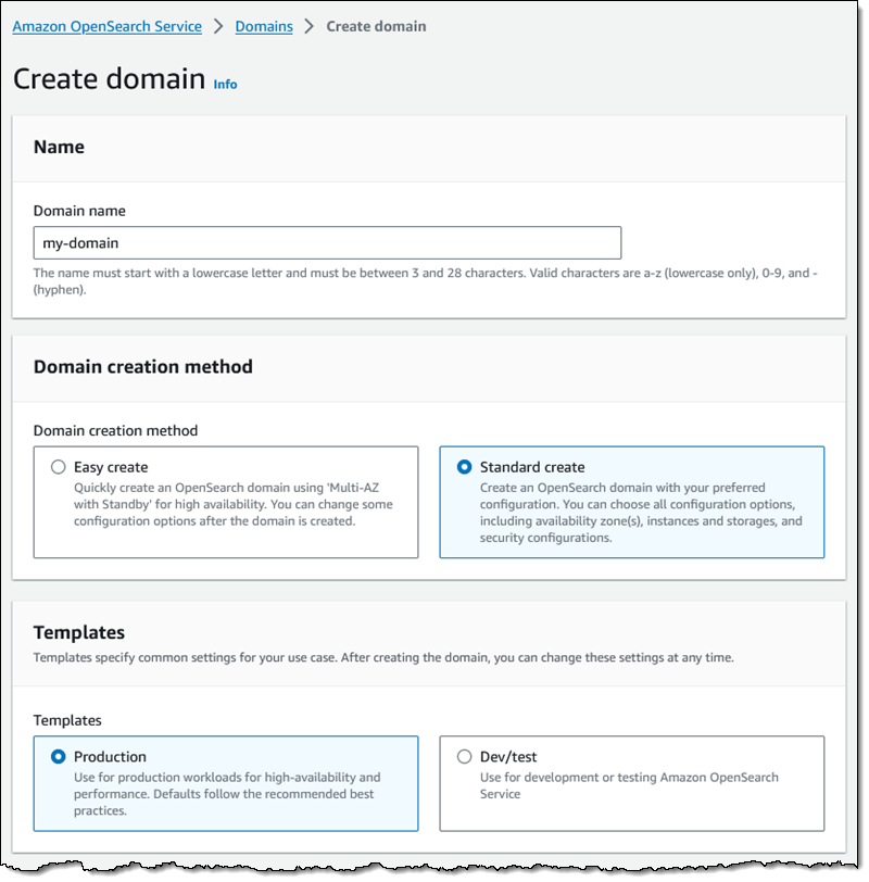
Then I choose the Domain with standby deployment option. This option will create active data nodes in two Availability Zones and a standby one in a third. I also choose the latest engine version:

Then I select the OR1 instance family and (for my use case) configure 500 GiB of EBS storage per data node:

I set the other settings as needed, and click Create to proceed:

I take a quick lunch break and when i come back my domain is ready:
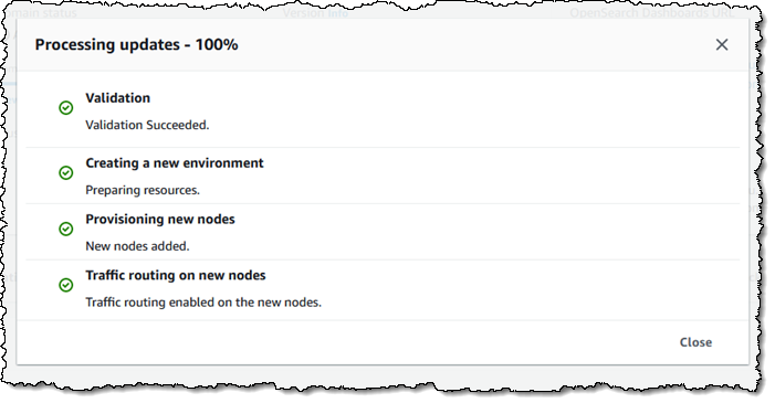
Things to Know
Here are a couple of things to know about this new storage option:
Engine Versions – Amazon OpenSearch Service engines version 2.11 and above support OR1 instances.
Regions – The OR1 instance family is available for use with OpenSearch in the US East (Ohio, N. Virginia), US West (N. California, Oregon), Asia Pacific (Mumbai, Singapore, Sydney, Tokyo), and Europe (Frankfurt, Ireland, Spain, Stockholm) AWS Regions.
Pricing – You pay On-Demand or Reserved prices for data nodes, and you also pay for EBS storage. See the Amazon OpenSearch Service Pricing page for more information.
— Jeff;
Unlocking the value of data as your differentiator
Post Syndicated from G2 Krishnamoorthy original https://aws.amazon.com/blogs/big-data/unlocking-the-value-of-data-as-your-differentiator/

Today on the AWS re:Invent keynote stage, Swami Sivasubramanian, VP of Data and AI, AWS, spoke about the beneficial relationship among data, generative AI, and humans—all working together to unleash new possibilities in efficiency and creativity. There has never been a more exciting time in modern technology. Innovation is accelerating everywhere, and the future is rife with possibility. While Swami explored many facets of this beneficial relationship in the keynote today, one area that is especially critical for our customers to get right if they want to see success in generative AI is data. When you want to build generative AI applications that are unique to your business needs, data is the differentiator. This week, we launched many new tools to help you turn your data into your differentiator. This includes tools to help you customize your foundation models, and new services and features to build a strong data foundation to fuel your generative AI applications.
Customizing foundation models
The need for data is quite obvious if you are building your own foundation models (FMs). These models need vast amounts of data. But data is necessary even when you are building on top of FMs. If you think about it, everyone has access to the same models for building generative AI applications. It’s data that is the key to moving from generic applications to generative AI applications that create real value for your customers and your business. For instance, Intuit’s new generative AI-powered assistant, Intuit Assist, uses relevant contextual datasets spanning small business, consumer finance, and tax information to deliver personalized financial insights to their customers. With Amazon Bedrock, you can privately customize FMs for your specific use case using a small set of your own labeled data through a visual interface without writing any code. Today, we announced the ability to fine-tune Cohere Command and Meta Llama 2 in addition to Amazon Titan. In addition to fine-tuning, we’re also making it easier for you to provide models with up-to-date and contextually relevant information from your data sources using Retrieval Augmented Generation (RAG). Amazon Bedrock’s Knowledge Bases feature, which went to general availability today, supports the entire RAG workflow, from ingestion, to retrieval, and prompt augmentation. Knowledge Bases works with popular vector databases and engines including Amazon OpenSearch Serverless, Redis Enterprise Cloud, and Pinecone, with support for Amazon Aurora and MongoDB coming soon.
Building a strong data foundation
To produce the high-quality data that you need to build or customize FMs for generative AI, you need a strong data foundation. Of course, the value of a strong data foundation is not new and the need for one spans well beyond generative AI. Across all types of use cases, from generative AI to business intelligence (BI), we’ve found that a strong data foundation includes a comprehensive set of services to meet all your use case needs, integrations across those services to break down data silos, and tools to govern data across the end-to-end data workflow so you can innovate more quickly. These tools also need to be intelligent to remove the heavy lifting from data management.
Comprehensive
First, you need a comprehensive set of data services so you can get the price/performance, speed, flexibility, and capabilities for any use case. AWS offers a broad set of tools that enable you to store, organize, access, and act upon various types of data. We have the broadest selection of database services, including relational databases like Aurora and Amazon Relational Database Service (Amazon RDS)—and on Monday, we introduced the newest addition to the RDS family: Amazon RDS for Db2. Now Db2 customers can easily set up, operate, and scale highly available Db2 databases in the cloud. We also offer non-relational databases like Amazon DynamoDB, used by over 1 million customers for its serverless, single-digit millisecond performance at any scale. You also need services to store data for analysis and machine learning (ML) like Amazon Simple Storage Service (Amazon S3). Customers have created hundreds of thousands of data lakes on Amazon S3. It also includes our data warehouse, Amazon Redshift, which delivers more than 6 times better price/performance than other cloud data warehouses. We also have tools that enable you to act on your data, including Amazon QuickSight for BI, Amazon SageMaker for ML, and of course, Amazon Bedrock for generative AI.

Serverless enhancements
The dynamic nature of data makes it perfectly suited to serverless technologies, which is why AWS offers a broad range of serverless database and analytics offerings that help support our customers’ most demanding workloads. This week, we made even more improvements to our serverless options in this area, including a new Aurora capability that automatically scales to millions of write transactions per second and manages petabytes of data while maintaining the simplicity of operating a single database. We also released a new serverless option for Amazon ElastiCache, which makes it faster and easier to create highly available caches and instantly scales to meet application demand. Finally, we announced new AI-driven scaling and optimizations for Amazon Redshift Serverless that enable the service to learn from your patterns and proactively scale on multiple dimensions, including concurrent users, data variability, and query complexity. It does all of this while factoring in your price/performance targets so you can optimize between cost and performance.
Vector capabilities across more databases
Your data foundation also needs to include services to store, index, retrieve, and search vector data. As our customers need vector embeddings as part as part of their generative AI application workflows, they told us they want to use vector capabilities in their existing databases to eliminate the steep learning curve for new programming tools, APIs, and SDKs. They also feel more confident knowing their existing databases are proven in production and meet requirements for scalability, availability, and storage and compute. And when your vectors and business data are stored in the same place, your applications will run faster—and there’s no data sync or data movement to worry about.
For all of these reasons, we’ve invested in adding vector capabilities to some of our most popular data services, including Amazon OpenSearch Service and OpenSearch Serverless, Aurora, and Amazon RDS. Today, we added four more to that list, with the addition of vector support in Amazon MemoryDB for Redis, Amazon DocumentDB (with MongoDB compatibility), DynamoDB, and Amazon Neptune. Now you can use vectors and generative AI with your database of choice.
Integrated
Another key to your data foundation is integrating data across your data sources for a more complete view of your business. Typically, connecting data across different data sources requires complex extract, transform, and load (ETL) pipelines, which can take hours—if not days—to build. These pipelines also have to be continuously maintained and can be brittle. AWS is investing in a zero-ETL future so you can quickly and easily connect and act on all your data, no matter where it lives. We’re delivering on this vision in a number of ways, including zero-ETL integrations between our most popular data stores. Earlier this year, we brought you our fully managed zero-ETL integration between Amazon Aurora MySQL-Compatible Edition and Amazon Redshift. Within seconds of data being written into Aurora, you can use Amazon Redshift to do near-real-time analytics and ML on petabytes of data. Woolworths, a pioneer in retail who helped build the retail model of today, was able to reduce development time for analysis of promotions and other events from 2 months to 1 day using the Aurora zero-ETL integration with Amazon Redshift.
More zero-ETL options
At re:Invent, we announced three more zero-ETL integrations with Amazon Redshift, including Amazon Aurora PostgreSQL-Compatible Edition, Amazon RDS for MySQL, and DynamoDB, to make it easier for you to take advantage of near-real-time analytics to improve your business outcomes. In addition to Amazon Redshift, we’ve also expanded our zero ETL support to OpenSearch Service, which tens of thousands of customers use for real-time search, monitoring, and analysis of business and operational data. This includes zero-ETL integrations with DynamoDB and Amazon S3. With all of these zero-ETL integrations, we’re making it even easier to leverage relevant data for your applications, including generative AI.
Governed
Finally, your data foundation needs to be secure and governed to ensure the data that’s used throughout the development cycle of your generative AI applications is high quality and compliant. To help with this, we launched Amazon DataZone last year. Amazon DataZone is being used by companies like Guardant Health and Bristol Meyers Squibb to catalog, discover, share, and govern data across their organization. Amazon DataZone uses ML to automatically add metadata to your data catalog, making all of your data more discoverable. This week, we added a new feature to Amazon DataZone that uses generative AI to automatically create business descriptions and context for your datasets with just a few clicks, making data even easier to understand and apply. While Amazon DataZone helps you share data in a governed way within your organization, many customers also want to securely share data with their partners.
Infusing intelligence across the data foundation
Not only have we added generative AI to Amazon DataZone, but we’re leveraging intelligent technology across our data services to make data easier to use, more intuitive to work with, and more accessible. Amazon Q, our new generative AI assistant, helps you in QuickSight to author dashboards and create compelling visual stories from your dashboard data using natural language. We also announced that Amazon Q can help you create data integration pipelines using natural language. For example, you can ask Q to “read JSON files from S3, join on ‘accountid’, and load into DynamoDB,” and Q will return an end-to-end data integration job to perform this action. Amazon Q is also making it easier to query data in your data warehouse with generative AI SQL in Amazon Redshift Query Editor (in preview). Now data analysts, scientists, and engineers can be more productive using generative AI text-to-code functionality. You can also improve accuracy by enabling query history access to specific users—without compromising data privacy.
These new innovations are going to make it easy for you to leverage data to differentiate your generative AI applications and create new value for your customers and your business. We look forward to seeing what you create!
About the authors
 G2 Krishnamoorthy is VP of Analytics, leading AWS data lake services, data integration, Amazon OpenSearch Service, and Amazon QuickSight. Prior to his current role, G2 built and ran the Analytics and ML Platform at Facebook/Meta, and built various parts of the SQL Server database, Azure Analytics, and Azure ML at Microsoft.
 Rahul Pathak is VP of Relational Database Engines, leading Amazon Aurora, Amazon Redshift, and Amazon QLDB. Prior to his current role, he was VP of Analytics at AWS, where he worked across the entire AWS database portfolio. He has co-founded two companies, one focused on digital media analytics and the other on IP-geolocation.
Amazon SageMaker Clarify makes it easier to evaluate and select foundation models (preview)
Post Syndicated from Antje Barth original https://aws.amazon.com/blogs/aws/amazon-sagemaker-clarify-makes-it-easier-to-evaluate-and-select-foundation-models-preview/
I’m happy to share that Amazon SageMaker Clarify now supports foundation model (FM) evaluation (preview). As a data scientist or machine learning (ML) engineer, you can now use SageMaker Clarify to evaluate, compare, and select FMs in minutes based on metrics such as accuracy, robustness, creativity, factual knowledge, bias, and toxicity. This new capability adds to SageMaker Clarify’s existing ability to detect bias in ML data and models and explain model predictions.
The new capability provides both automatic and human-in-the-loop evaluations for large language models (LLMs) anywhere, including LLMs available in SageMaker JumpStart, as well as models trained and hosted outside of AWS. This removes the heavy lifting of finding the right model evaluation tools and integrating them into your development environment. It also simplifies the complexity of trying to adopt academic benchmarks to your generative artificial intelligence (AI) use case.
Evaluate FMs with SageMaker Clarify
With SageMaker Clarify, you now have a single place to evaluate and compare any LLM based on predefined criteria during model selection and throughout the model customization workflow. In addition to automatic evaluation, you can also use the human-in-the-loop capabilities to set up human reviews for more subjective criteria, such as helpfulness, creative intent, and style, by using your own workforce or managed workforce from SageMaker Ground Truth.
To get started with model evaluations, you can use curated prompt datasets that are purpose-built for common LLM tasks, including open-ended text generation, text summarization, question answering (Q&A), and classification. You can also extend the model evaluation with your own custom prompt datasets and metrics for your specific use case. Human-in-the-loop evaluations can be used for any task and evaluation metric. After each evaluation job, you receive an evaluation report that summarizes the results in natural language and includes visualizations and examples. You can download all metrics and reports and also integrate model evaluations into SageMaker MLOps workflows.
In SageMaker Studio, you can find Model evaluation under Jobs in the left menu. You can also select Evaluate directly from the model details page of any LLM in SageMaker JumpStart.

Select Evaluate a model to set up the evaluation job. The UI wizard will guide you through the selection of automatic or human evaluation, model(s), relevant tasks, metrics, prompt datasets, and review teams.

Once the model evaluation job is complete, you can view the results in the evaluation report.

In addition to the UI, you can also start with example Jupyter notebooks that walk you through step-by-step instructions on how to programmatically run model evaluation in SageMaker.
Evaluate models anywhere with the FMEval open source library
To run model evaluation anywhere, including models trained and hosted outside of AWS, use the FMEval open source library. The following example demonstrates how to use the library to evaluate a custom model by extending the ModelRunner class.
For this demo, I choose GPT-2 from the Hugging Face model hub and define a custom HFModelConfig and HuggingFaceCausalLLMModelRunner class that works with causal decoder-only models from the Hugging Face model hub such as GPT-2. The example is also available in the FMEval GitHub repo.
!pip install fmeval

# ModelRunners invoke FMs
from amazon_fmeval.model_runners.model_runner import ModelRunner

# Additional imports for custom model
import warnings
from dataclasses import dataclass
from typing import Tuple, Optional
import torch
from transformers import AutoModelForCausalLM, AutoTokenizer

@dataclass
class HFModelConfig:
    model_name: str
    max_new_tokens: int
    normalize_probabilities: bool = False
    seed: int = 0
    remove_prompt_from_generated_text: bool = True

class HuggingFaceCausalLLMModelRunner(ModelRunner):
    def __init__(self, model_config: HFModelConfig):
        self.config = model_config
        self.model = AutoModelForCausalLM.from_pretrained(self.config.model_name)
        self.tokenizer = AutoTokenizer.from_pretrained(self.config.model_name)

    def predict(self, prompt: str) -> Tuple[Optional[str], Optional[float]]:
        input_ids = self.tokenizer(prompt, return_tensors="pt").to(self.model.device)
        generations = self.model.generate(
            **input_ids,
            max_new_tokens=self.config.max_new_tokens,
            pad_token_id=self.tokenizer.eos_token_id,
        )
        generation_contains_input = (
            input_ids["input_ids"][0] == generations[0][: input_ids["input_ids"].shape[1]]
        ).all()
        if self.config.remove_prompt_from_generated_text and not generation_contains_input:
            warnings.warn(
                "Your model does not return the prompt as part of its generations. "
                "`remove_prompt_from_generated_text` does nothing."
            )
        if self.config.remove_prompt_from_generated_text and generation_contains_input:
            output = self.tokenizer.batch_decode(generations[:, input_ids["input_ids"].shape[1] :])[0]
        else:
            output = self.tokenizer.batch_decode(generations, skip_special_tokens=True)[0]

        with torch.inference_mode():
            input_ids = self.tokenizer(self.tokenizer.bos_token + prompt, return_tensors="pt")["input_ids"]
            model_output = self.model(input_ids, labels=input_ids)
            probability = -model_output[0].item()

        return output, probability
Next, create an instance of HFModelConfig and HuggingFaceCausalLLMModelRunner with the model information.
Then, select and configure the evaluation algorithm.
Let’s first test with one sample. The evaluation score is the percentage of factually correct responses.
Although it’s not a perfect response, it includes “UK.”
Next, you can evaluate the FM using built-in datasets or define your custom dataset. If you want to use a custom evaluation dataset, create an instance of DataConfig:
The evaluation results will return a combined evaluation score across the dataset and detailed results for each model input stored in a local output path.
Join the preview
FM evaluation with Amazon SageMaker Clarify is available today in public preview in AWS Regions US East (Ohio), US East (N. Virginia), US West (Oregon), Asia Pacific (Singapore), Asia Pacific (Tokyo), Europe (Frankfurt), and Europe (Ireland). The FMEval open source library] is available on GitHub. To learn more, visit Amazon SageMaker Clarify.
Get started
Log in to the AWS Management Console and start evaluating your FMs with SageMaker Clarify today!
— Antje