Universities and colleges lead the way in educating future professionals and conducting ground-breaking research. Altogether, higher education generates hundreds of terabytes—even petabytes—of data. But, higher education also faces significant data risks. They are one of the most targeted industries for ransomware, with 79% of institutions reporting they were hit with ransomware in the past year.
While higher education institutions often have robust data storage systems that can even include their own off-site disaster recovery (DR) centers, cloud storage can provide several benefits that legacy storage systems cannot match. In particular, cloud storage allows schools to protect from ransomware with immutability, easily grow their datasets without constant hardware outlays, and protect faculty, student, and researchers’ computers with cloud-based endpoint backups.
Cloud storage is also a promising alternative to cloud drives, traditionally a popular option for higher education institutions. While cloud drives provide easy storage across campus, both Google and Microsoft have announced the end of their unlimited storage tiers for education. Faced with changes to the original service, many higher education institutions are looking for alternatives. Plus, cloud drives do not provide true, incremental backup, do not adequately protect from ransomware, and have limited options for recovery.
Ultimately, cloud storage better protects your school from local disasters and ransomware with a secure, off-site copy of your data. And, with the right cloud service provider, it can be much more affordable than you think. In this article, we’ll look at the benefits of cloud storage for higher education, study some popular use cases, and explore best practices and provisioning considerations.
The Benefits of Cloud Storage in Higher Education
Cloud storage solutions present a host of benefits for organizations in any industry, but many of these benefits are particularly relevant for higher education institutions. Let’s take a look:
1. Enhanced Security
Higher education institutions have emerged as one of ransomware attackers’ favorite targets—63% of higher education CISOs say a cyber attack is likely within the next year. Data backups are a core part of any organization’s security posture, and that includes keeping those backups protected and secure in the cloud. Using cloud storage to store backups strengthens backup programs by keeping copies off-site and geographically distanced, which adheres to the 3-2-1 backup strategy (more on that later). Cloud storage can also be made immutable using tools like Object Lock, meaning data can’t be modified or deleted. This feature is often unavailable in existing data storage hardware.
2. Cost-Effective Storage
Higher education generates huge volumes of data each year. Keeping costs low without sacrificing in other areas is a key priority for these institutions, across both active data and archival data stores. Cloud storage helps higher education institutions use their storage budgets effectively by not paying to provision and maintain on-premises infrastructure they don’t need. It can also help higher education institutions migrate away from linear tape-open (LTO) which can be costly to manage.
3. Improved Scalability
As digital data continues to grow, it’s important for those institutions to be able to easily scale with their storage needs. Cloud storage allows higher education institutions to avoid potentially over-provisioning infrastructure with the ability to affordably tier off data to the cloud.
4. Data Accessibility
Making data easily accessible is important for many aspects of higher education. From the impact of scientific researchers to the ongoing work of attracting students to the university, the increasing quantities of data that higher education creates needs to be easy to access, use, and manage. Cloud storage makes data accessible from anywhere, and with hot cloud storage, there are no access delays like there can be with cold cloud storage or LTO tape.
5. Supports Cybersecurity Insurance Requirements
It’s increasingly common to utilize cyber insurance to offset potential liabilities incurred by a cyber attack. Many of those applications ask if the covered entity has off-site backups or immutable backups. Sometimes they even specify the backup has to be held somewhere other than the organization’s own locations. (We’ve seen other organizations outside of higher ed adding cloud storage for this reason as well). Cloud storage provides a pathway to meeting cyber insurance requirements universities may face.
How Higher Ed Institutions Can Use Cloud Storage Effectively
There are many ways higher education institutions can make effective use of cloud storage solutions. The most common use case is cloud storage for backup and archive systems. Transitioning from on-premises storage to cloud-based solutions—even if an organization is only transitioning a part of their total data footprint while retaining on-premises systems—is a powerful way for higher education institutions to protect their most important data. To illustrate, here are some common use cases with real-life examples:
LTO Replacement
It’s no surprise that maintaining tape is a pain. While it’s the only true physical air-gap solution, it’s also a time suck, and those are precious hours that your IT team should be spending on strategic initiatives. This is particularly applicable in projects that generate huge amounts of data, like scientific research. Cloud storage provides the same off-site protection as LTO with far fewer maintenance hours.
Off-Site Backups
As mentioned, higher ed institutions often keep an off-site copy of their data, but it’s commonly a few miles down the road—perhaps at a different branch’s campus. Transitioning to cloud storage allowed Coast Community College District (CCCD) to quit chauffeuring physical tapes to an off-site backup center about five miles away and instead implement a virtualized, multi-cloud solution with truly geographically distanced backups.
Protection From Ransomware
A ransomware attack is not a matter of if, but when. Cloud storage provides immutable ransomware protection with Object Lock, which creates a “virtual” air gap. Pittsburg State University, for example, leverages cloud storage to protect university data from ransomware threats. They strengthened their protection four-fold by adding immutable off-site data backups, and are now able to manage data recovery and data integrity with a single robust solution (that doesn’t multiply their expenses).
Computer Backup
While S3 compatible object storage provides a secure destination for data from servers, virtual machines (VMs), and network attached storage (NAS), it’s important to remember to back up faculty, staff, student, and researchers’ computers as well. Workstation backup is particularly important for organizations that are leveraging cloud drives, as these platforms are only designed to capture data stored in their respective clouds, leaving local files vulnerable to loss. But, one thing you don’t want is a drain on your IT resources—you want a solution that’s easy to implement, easy to manage ongoing, and simple enough to serve users of varying tech savviness.
Best Practices for Data Backup and Management in the Cloud
Higher education institutions (and anyone, really!) should follow basic best practices to get the most out of their cloud storage solutions. Here are a few key points to keep in mind when developing a data backup and management strategy for higher education:
The 3-2-1 Backup Strategy
This widely accepted foundational structure recommends keeping three copies of all important data (one primary copy and two backup copies) on two different media types (to diversify risk) and storing at least one copy off-site. While colleges and universities frequently have high-capacity data storage systems, they don’t always adhere to the 3-2-1 rule. For instance, a school may have an off-site disaster recovery site, but their backups are not on two different media types. Or, they may be meeting the two-media-type rule but their media are not wholly off-site. Keeping your backups at a different campus location does not constitute a true off-site backup if you’re in the same region, for instance—the closer your data storage sites are, the more likely they’ll be subject to the same risks, like network outages, natural disasters, and so on.
Regular Data Backups
You’re only as strong as your last backup. Maintaining a frequent and regular backup schedule is a tried and true way to ensure that your institution’s data is as protected as possible. Schools that have historically relied on Google Drive, Dropbox, OneDrive, and other cloud drive systems are particularly vulnerable to this gap in their data protection strategy. Cloud drives provide sync functionality; they are not a true backup. While many now have the ability to restore files, restore periods are limited and not customizable and services often only back up certain file types—so, your documents, but not your email or user data, for instance. Especially when you’re talking about larger organizations with complex file management and high compliance needs, they don’t provide adequate protection from ransomware. Speaking of ransomware…
Ransomware Protection
Educational institutions (including both K-12 and higher ed) are more frequently targeted by ransomware today than ever before. When you’re using cloud storage, you can enable security features like Object Lock to offer “air gapped” protection and data immutability in the cloud. When you add endpoint backup, you’re ensuring that all the data on a workstation is backed up—closing a gap in cloud drives that can leave certain types of data vulnerable to loss.
Disaster Recovery Planning
Incorporating cloud storage into your disaster recovery strategy is the best way to plan for the worst. If unexpected disasters occur, you’ll know exactly where your data lives and how to restore it so you can get back to work quickly. Schools will often use cross-site replication as their disaster recovery solution, but such methods can fail the 3-2-1 test (see above) and it’s not a true backup since replication functions much the same way as sync. If ransomware invades your primary dataset, it can be replicated across all your copies. Cloud storage allows you to fortify your disaster recovery strategy and plug the gaps in your data protection.
Regulatory Compliance
Universities work with and store many diverse kinds of information, including highly regulated data types like medical records and research data. It’s important for higher education to use cloud storage solutions that help them remain in compliance with data privacy laws and federal or international regulations. Providers like Backblaze that frequently work with higher education institutions will usually have a HECVAT questionnaire available so you can better understand a vendor’s compliance and security stance, and they go through regular compliance audits via regulatory agencies like StateRAMP or SOC-2 certifications.
Comprehensive Protection
While it’s obvious that data systems like servers, virtual machines, and network attached storage (NAS) should be backed up, consider the other important sources of data that should be included in your protection strategy. For instance, your Microsoft 365 data should be backed up because you cannot rely on Microsoft to provide adequate backups. Under the shared responsibility model, Microsoft and other SaaS providers state that your data is your responsibility to back up—even if it’s stored on their cloud. And don’t forget about your faculty, student, staff, and researchers’ computers. These devices can hold incredibly valuable work and having a native endpoint backup solution is critical.
The Importance of Cloud Storage for Higher Education Institutions
Institutions of higher education were already on the long road toward digital transformation before the pandemic hit, but 2020 forced any reluctant parties to accept that the future was upon us. The combination of schools’ increasing quantities of sensitive and protected data and the growing threat of ransomware in the higher education space reinforce the need for secure and robust cloud storage solutions. As time has gone on, it’s clear that the diverse needs of higher education institutions need flexible, scalable, affordable solutions, and that current and legacy solutions have room for improvement.
Universities that leverage best practices like designing 3-2-1 backup strategies, conducting frequent and regular backups, and developing disaster recovery plans before they’re needed will be well on their way toward becoming more modern, digital-first organizations. And with the right cloud storage solutions in place, they’ll be able to move the needle with measurable business benefits like cost effectiveness, data accessibility, increased security, and scalability.
Amazon Redshift is a fast, fully managed, petabyte-scale data warehouse service that makes it simple and cost-effective to analyze all your data efficiently and securely. Users such as data analysts, database developers, and data scientists use SQL to analyze their data in Amazon Redshift data warehouses. Amazon Redshift provides a web-based Query Editor V2 in addition to supporting connectivity via ODBC/JDBC or the Amazon Redshift Data API.
Amazon Redshift Query Editor V2 makes it easy to query your data using SQL and gain insights by visualizing your results using charts and graphs with a few clicks. With Query Editor V2, you can collaborate with team members by easily sharing saved queries, results, and analyses in a secure way.
Analysts performing ad hoc analyses in their workspace need to load sample data in Amazon Redshift by creating a table and load data from desktop. They want to join that data with the curated data in their data warehouse. Data engineers and data scientists have test data, and want to load data into Amazon Redshift for their machine learning (ML) or analytics use cases.
In this post, we walk through a new feature in Query Editor V2 to easily load data files either from your local desktop or Amazon Simple Storage Service (Amazon S3).
AmazonRedshiftQueryEditorV2FullAccess – Grants full access to the Query Editor V2 operations and resources.
AmazonRedshiftQueryEditorV2NoSharing – Grants the ability to work with Query Editor V2 without sharing resources.
AmazonRedshiftQueryEditorV2ReadSharing – Grants the ability to work with Query Editor V2 with limited sharing of resources. The granted principal can read the resources shared with its team but can’t update them.
AmazonRedshiftQueryEditorV2ReadWriteSharing – Grants the ability to work with Query Editor V2 with sharing of resources. The granted principal can read and update the resources shared with its team.
Provide access to the S3 bucket to load data from a local desktop file.
To enable your users to load data from a local desktop using Query Editor V2, as an administrator, you have to specify a common S3 bucket, and the user account must be configured with proper permissions. You can use the following IAM policy as an example to configure your IAM user or role:
It’s also recommended to have proper separation of data access when loading data files from your local desktop. You can use the following S3 bucket policy as an example to separate data access between users of the staging bucket you configured:
As an admin, you must first configure Query Editor V2 before providing access to your end-users. On the Amazon Redshift console, choose Query editor v2 in the navigation pane.
If you’re accessing Query Editor v2 for the first time, you must configure your account by providing AWS Key Management Service (AWS KMS) encryption and, optionally, an S3 bucket.
By default, an AWS-owned key is used to encrypt resources. Optionally, you can create a symmetric customer managed key to encrypt Query Editor V2 resources such as saved queries and query results using the AWS KMS console or AWS KMS API operations.
The S3 bucket URI is required when loading data from your local desktop. You can provide the S3 URI of the same bucket that you configured earlier as a prerequisite.
If you have previously configured Query Editor V2 with only AWS KMS encryption, you can choose Account Settings after launching the interface to update the S3 URI to support loading from your local desktop.
Load data from your local desktop
Users such as data analysts, database developers, and data scientists can now load local files up to 5 MB in size into Amazon Redshift tables from Query Editor V2, without using the COPY command. The supported data formats are CSV, JSON, DELIMITER, FIXEDWIDTH, SHAPEFILE, AVRO, PARQUET, and ORC. Complete the following steps:
On the Amazon Redshift console, navigate to Query Editor V2.
Click on Load data.
Choose Load from local file and Browse to choose a local file. You can download the student_info.csv file to use as an example.
If your file has column headers as the first row, keep the default selection of Ignore header rows as 1 to ignore first row.
If your file has date columns, choose Data conversion parameters.
Select Date format, set it to auto and choose Next.
Choose Load new table to automatically infer the file schema.
Specify the values for Cluster or workgroup, Database, Schema, and Table (for example, Student_info) to load data to.
Choose Create table.
A success message appears that the table was created. Now you can load data into the newly created table from a local file.
Choose Load data.
A message appears that the data load was successful.
Query the Student_info table to see the data.
Load data from Amazon S3
You can easily load data from Amazon S3 into an Amazon Redshift table using Query Editor V2. Complete the following steps:
On the Amazon Redshift console, launch Query Editor V2 and connect to your cluster.
Browse to the database name (for example, dev), the public schema, and expand Tables.
You can automatically infer the schema of a S3 file similar to Load from local file option shown above however for this demo, we will also show you how to load data to an existing table. Run the following create table script to make a sample table (for this example, public.customer):
CREATE TABLE customer (
	c_custkey int8 NOT NULL ,
	c_name varchar(25) NOT NULL,
	c_address varchar(40) NOT NULL,
	c_nationkey int4 NOT NULL,
	c_phone char(15) NOT NULL,
	c_acctbal numeric(12,2) NOT NULL,
	c_mktsegment char(10) NOT NULL,
	c_comment varchar(117) NOT NULL,
PRIMARY Key(C_CUSTKEY)
) DISTKEY(c_custkey) sortkey(c_custkey);
Choose Load data.
Choose Load from S3 bucket.
For this post, we load data from the TPCH Sample data GitHub repo, so for the S3 URI, enter s3://redshift-downloads/TPC-H/2.18/10GB/customer.tbl.
For S3 file location, choose us-east-1.
For File format, choose Delimiter.
For Delimiter character, enter |.
Choose Data conversion parameters, then select Time format and Date format as auto.
Specify the Cluster or workgroup, Database, Schema (for example, public) and Table name (for example, customer).
For IAM role, choose a suitable IAM role.
Choose Load data.
Query Editor V2 generates the COPY command and runs it on the Amazon Redshift cluster. The results of the COPY command are displayed in the Result section upon completion.
Conclusion
In this post, we showed how Amazon Redshift Query Editor V2 has simplified the process to load data into Amazon Redshift from Amazon S3 or your local desktop, thereby accelerating the data analysis. It’s an easy-to-use feature that your teams can start using to load and query datasets. If you have any questions or suggestions, please leave a comment.
About the Authors
Raks Khare is an Analytics Specialist Solutions Architect at AWS based out of Pennsylvania. He helps customers architect data analytics solutions at scale on the AWS platform.
Tahir Aziz is an Analytics Solution Architect at AWS. He has worked with building data warehouses and big data solutions for over 13 years. He loves to help customers design end-to-end analytics solutions on AWS. Outside of work, he enjoys traveling and cooking.
Erol Murtezaoglu, a Technical Product Manager at AWS, is an inquisitive and enthusiastic thinker with a drive for self-improvement and learning. He has a strong and proven technical background in software development and architecture, balanced with a drive to deliver commercially successful products. Erol highly values the process of understanding customer needs and problems, in order to deliver solutions that exceed expectations.
Sapna Maheshwari is a Sr. Solutions Architect at Amazon Web Services. She has over 18 years of experience in data and analytics. She is passionate about telling stories with data and enjoys creating engaging visuals to unearth actionable insights.
Karthik Ramanathan is a Software Engineer with Amazon Redshift and is based in San Francisco. He brings close to two decades of development experience across the networking, data storage and IoT verticals. When not at work he is also a writer and loves to be in the water.
Albert Harkema is a Software Development Engineer at AWS. He is known for his curiosity and deep-seated desire to understand the inner workings of complex systems. His inquisitive nature drives him to develop software solutions that make life easier for others. Albert’s approach to problem-solving emphasizes efficiency, reliability, and long-term stability, ensuring that his work has a tangible impact. Through his professional experiences, he has discovered the potential of technology to improve everyday life.
Amazon Managed Workflows for Apache Airflow (Amazon MWAA) is a managed orchestration service for Apache Airflow that makes it simple to set up and operate end-to-end data pipelines in the cloud at scale. Amazon MWAA supports multiple versions of Apache Airflow (v1.10.12, v2.0.2, and v2.2.2). Earlier in 2023, we added support for Apache Airflow v2.4.3 so you can enjoy the same scalability, availability, security, and ease of management with Airflow’s most recent improvements. Additionally, with Apache Airflow v2.4.3 support, Amazon MWAA has upgraded to Python v3.10.8, which supports newer Python libraries like OpenSSL 1.1.1 as well as major new features and improvements.
In this post, we provide an overview of the features and capabilities of Apache Airflow v2.4.3 and how you can set up or upgrade your Amazon MWAA environment to accommodate Apache Airflow v2.4.3 as you orchestrate using workflows in the cloud at scale.
New feature: Data-aware scheduling using datasets
With the release of Apache Airflow v2.4.0, Airflow introduced datasets. An Airflow dataset is a stand-in for a logical grouping of data that can trigger a Directed Acyclic Graph (DAG) in addition to regular DAG triggering mechanisms such as cron expressions, timedelta objects, and Airflow timetables. The following are some of the attributes of a dataset:
Datasets may be updated by upstream producer tasks, and updates to such datasets contribute to scheduling downstream consumer DAGs.
You can create smaller, more self-contained DAGs, which chain together into a larger data-based workflow using datasets.
You have an additional option now to create inter-DAG dependencies using datasets besides ExternalTaskSensor or TriggerDagRunOperator. You should consider using this dependency if you have two DAGs related via an irregular dataset update. This type of dependency also provides you with increased observability into the dependencies between your DAGs and datasets in the Airflow UI.
How data-aware scheduling works
You need to define three things:
A dataset, or multiple datasets
The tasks that will update the dataset
The DAG that will be scheduled when one or more datasets are updated
The following diagram illustrates the workflow.
The producer DAG has a task that creates or updates the dataset defined by a Uniform Resource Identifier (URI). Airflow schedules the consumer DAG after the dataset has been updated. A dataset will be marked as updated only if the producer task completes successfully—if the task fails or if it’s skipped, no update occurs, and the consumer DAG will not be scheduled. If your updates to a dataset triggers multiple subsequent DAGs, then you can use the Airflow metric max_active_tasks_per_dag to control the parallelism of the consumer DAG and reduce the chance of overloading the system.
Let’s demonstrate this with a code example.
Prerequisites to build a data-aware scheduled DAG
You must have the following prerequisites:
An Amazon Simple Storage Service (Amazon S3) bucket to upload datasets in. This can be a separate prefix in your existing S3 bucket configured for your Amazon MWAA environment, or it can be a completely different S3 bucket that you identify to store your data in.
An Amazon MWAA environment configured with Apache Airflow v2.4.3. The Amazon MWAA execution role should have access to read and write to the S3 bucket configured to upload datasets. The latter is only needed if it’s a different bucket than the Amazon MWAA bucket.
The following diagram illustrates the solution architecture.
The workflow steps are as follows:
The producer DAG makes an API call to a publicly hosted API to retrieve data.
After the data has been retrieved, it’s stored in the S3 bucket.
The update to this dataset subsequently triggers the consumer DAG.
You can access the producer and consumer code in the GitHub repo.
Test the feature
To test this feature, run the producer DAG. After it’s complete, verify that a file named test.csv is generated in the specified S3 folder. Verify in the Airflow UI that the consumer DAG has been triggered by updates to the dataset and that it runs to completion.
There are two restrictions on the dataset URI:
It must be a valid URI, which means it must be composed of only ASCII characters
The URI scheme can’t be an Airflow scheme (this is reserved for future use)
Other notable changes in Apache Airflow v2.4.3:
Apache Airflow v2.4.3 has the following additional changes:
Deprecation of schedule_interval and timetable arguments. Airflow v2.4.0 added a new DAG argument schedule that can accept a cron expression, timedelta object, timetable object, or list of dataset objects.
Removal of experimental Smart Sensors. Smart Sensors were added in v2.0 and were deprecated in favor of deferrable operators in v2.2, and have now been removed. Deferrable operators are not yet supported on Amazon MWAA, but will be offered in a future release.
Implementation of ExternalPythonOperator that can help you run some of your tasks with a different set of Python libraries than other tasks (and other than the main Airflow environment).
Dynamic task mapping was a new feature introduced in Apache Airflow v2.3, which has also been extended in v2.4. Dynamic task mapping lets DAG authors create tasks dynamically based on current data. Previously, DAG authors needed to know how many tasks were needed in advance.
This is similar to defining your tasks in a loop, but instead of having the DAG file fetch the data and do that itself, the scheduler can do this based on the output of a previous task. Right before a mapped task is run, the scheduler will create n copies of the task, one for each input. The following diagram illustrates this workflow.
It’s also possible to have a task operate on the collected output of a mapped task, commonly known as map and reduce. This feature is particularly useful if you want to externally process various files, evaluate multiple machine learning models, or extraneously process a varied amount of data based on a SQL request.
How dynamic task mapping works
Let’s see an example using the reference code available in the Airflow documentation.
The following code results in a DAG with n+1 tasks, with n mapped invocations of count_lines, each called to process line counts, and a total that is the sum of each of the count_lines. Here n represents the number of input files uploaded to the S3 bucket.
With n=4 files uploaded, the resulting DAG would look like the following figure.
Prerequisites to build a dynamic task mapped DAG
You need the following prerequisites:
An S3 bucket to upload files in. This can be a separate prefix in your existing S3 bucket configured for your Amazon MWAA environment, or it can be a completely different bucket that you identify to store your data in.
An Amazon MWAA environment configured with Apache Airflow v2.4.3. The Amazon MWAA execution role should have access to read to the S3 bucket configured to upload files. The latter is only needed if it’s a different bucket than the Amazon MWAA bucket.
Upload the four sample text files from the local data folder to an S3 bucket data folder. Run the dynamic_task_mapping DAG. When it’s complete, verify from the Airflow logs that the final sum is equal to the sum of the count lines of the individual files.
There are two limits that Airflow allows you to place on a task:
The number of mapped task instances that can be created as the result of expansion
With Apache Airflow v2.4.3 support, Amazon MWAA has upgraded to Python v3.10.8, providing support for newer Python libraries, features, and improvements. Python v3.10 has slots for data classes, match statements, clearer and better Union typing, parenthesized context managers, and structural pattern matching. Upgrading to Python v3.10 should also help you align with security standards by mitigating the risk of older versions of Python such as 3.7, which is fast approaching its end of security support.
With structural pattern matching in Python v3.10, you can now use switch-case statements instead of using if-else statements and dictionaries to simplify the code. Prior to Python v3.10, you might have used if statements, isinstance calls, exceptions and membership tests against objects, dictionaries, lists, tuples, and sets to verify that the structure of the data matches one or more patterns. The following code shows what an ad hoc pattern matching engine might have looked like prior to Python v3.10:
def http_error(status):
        if status == 200:
           return 'OK'
        elif status == 400:
            return 'Bad request'
 	    elif status == 401:
      	    return 'Not allowed'
	    elif status == 403:
      	    return 'Not allowed'
 	    elif status == 404:
      	    return 'Not allowed'
 	    else:
	        return 'Something is wrong'
With structural pattern matching in Python v3.10, the code is as follows:
def http_error(status):
    match status:
        case 200:
            return 'OK'
        case 400:
            return 'Bad request'
        case 401 | 403 | 404:
            return 'Not allowed'
        case _:
            return 'Something is wrong'
Python v3.10 also carries forward the performance improvements introduced in Python v3.9 using the vectorcall protocol. vectorcall makes many common function calls faster by minimizing or eliminating temporary objects created for the call. In Python 3.9, several Python built-ins—range, tuple, set, frozenset, list, dict—use vectorcall internally to speed up runs. The second big performance enhancer is more efficient in the parsing of Python source code using the new parser for the CPython runtime.
When you have successfully created an Apache Airflow v2.4.3 environment in Amazon MWAA, the following packages are automatically installed on the scheduler and worker nodes along with other provider packages:
apache-airflow-providers-amazon==6.0.0
python==3.10.8
For a complete list of provider packages installed, refer to Apache Airflow provider packages installed on Amazon MWAA environments. Note that some imports and operator names have changed in the new provider package in order to standardize the naming convention across the provider package. For a complete list of provider package changes, refer to the package changelog.
Upgrade from Apache Airflow v2.0.2 or v2.2.2 to Apache Airflow v2.4.3
Currently, Amazon MWAA doesn’t support in-place upgrades of existing environments for older Apache Airflow versions. In this section, we show how you can transfer your data from your existing Apache Airflow v2.0.2 or v2.2.2 environment to Apache Airflow v2.4.3:
Copy your DAGs, custom plugins, and requirements.txt resources from your existing v2.0.2 or v2.2.2 S3 bucket to the new environment’s S3 bucket.
If you use requirements.txt in your environment, you need to update the --constraint to v2.4.3 constraints and verify that the current libraries and packages are compatible with Apache Airflow v2.4.3
With Apache Airflow v2.4.3, the list of provider packages Amazon MWAA installs by default for your environment has changed. Note that some imports and operator names have changed in the new provider package in order to standardize the naming convention across the provider package. Compare the list of provider packages installed by default in Apache Airflow v2.2.2 or v2.0.2, and configure any additional packages you might need for your new v2.4.3 environment. It’s advised to use the aws-mwaa-local-runner utility to test out your new DAGs, requirements, plugins, and dependencies locally before deploying to Amazon MWAA.
Test your DAGs using the new Apache Airflow v2.4.3 environment.
If you plan to migrate existing metadata from your previous environments to the new one, perform the export and import steps detailed in Migrating to a new Amazon MWAA environment.
After you have confirmed that your tasks completed successfully, delete the v2.0.2 or v2.2.2 environment.
Conclusion
In this post, we talked about the new features of Apache Airflow v2.4.3 and how you can get started using it in Amazon MWAA. Try out these new features like data-aware scheduling, dynamic task mapping, and other enhancements along with Python v.3.10.
About the authors
Parnab Basak is a Solutions Architect and a Serverless Specialist at AWS. He specializes in creating new solutions that are cloud native using modern software development practices like serverless, DevOps, and analytics. Parnab works closely in the analytics and integration services space helping customers adopt AWS services for their workflow orchestration needs.
Not all MDR services are created equal, and in order for organizations to find the right partner for their managed detection and response needs, Gartner® has published a Market Guide report offering key insights for businesses of all sizes. At Rapid7, we are proud to offer this complimentary report and share our three key takeaways from it.
MDR services have skyrocketed over the past few years. In the report, Gartner says: “MDR is a high-growth, established market (see Market Share: Managed Security Services, Worldwide, 2021 where MDR is a distinct segment, the MDR market grew 48.9% from 2020 to 2021).”
Because of the high growth in the market, many managed security services use the term MDR. However, organizations looking for a true Managed Detection and Response partner, should look to the Gartner definition to identify the right vendor.
Gartner puts it this way: “MDR services provide customers with remotely delivered, humanled, turnkey, modern SOC functions; ultimately delivering threat disruption and containment.”
But choosing a strong MDR partner goes far beyond these high-level requirements. Below are our key takeaways from the report. Without further ado, let’s dive right in.
Takeaway 1: Beware Providers Mimicking MDR
The key to MDR lies as much in the human-centric nature of the service as the power of the technology behind it. Managed Detection and Response is just that… managed. It requires a human with expertise not only in understanding the detection and remediation of threats and breaches, but how these correlate to your business and its goals. Sadly, not all services claiming to be MDR lead with this human expertise.
Gartner shares: “Misnamed technology-centric offerings and vendor-delivered service wrappers (VDSW), that fail to deliver human-driven managed detection and response (MDR) services, are causing challenges for buyers looking to identify and select an outcome-driven provider.”
Human-analyzed context is critically important to the success of an MDR program and an organization’s outcomes in their security programs. Unfortunately, some providers are not living up to their own marketing materials. For instance, Gartner found that some “deliver a far less human-driven experience, depending on the technology for the bulk of the delivery. Although still valuable, these offerings are often promoted as being more engaged than they actually are and would be better described as managed EDR (MEDR).”
Takeaway 2: Context is King
This could be considered a corollary to the previous takeaway, but we acknowledge how important it is for an MDR provider to understand your organization’s unique environment, the context of threats, and how those threats have potential to impact your business. It is not enough to simply detect and remediate threats; an MDR SOC should understand which threats and types of threats will have the biggest impact on your company or organization.
The human-led nature of successful MDR programs means that a company can rest assured that their MDR SOC is able to provide insights that are actually useful to boost their customer’s outcomes.
Gartner has this to say on the subject: “MDR buyers must focus on the ability to provide context-driven insights that will directly impact their business objectives, as wide-scale collection of telemetry and automated analysis are insufficient when facing uncommon threats.”
We feel this has a direct relationship with the expertise of the MDR provider and the quality of the technology they are providing. Too much information without the context necessary to triage and prioritize could overwhelm any security team. Too little information and threats go unchecked. Finding the right balance between the tech and expertise is critical.
Takeaway 3: Threats Know No Boundaries
Ok, that subhead may be a little hyperbolic, but it should surprise no one that threat actors aren’t clocking out at 5pm on a Friday and taking holidays off. Your MDR SOC can’t either. Gartner recommends “Use MDR services to obtain 24/7, remotely delivered, human-led security operations capabilities when there are no existing internal capabilities, or when the organization needs to accelerate or augment existing security operations capabilities.”
So, what exactly does that mean? Essentially, any MDR SOC you choose should provide round-the-clock security that knows no geographical limitations, and has a team of experts actively detecting, assessing, and providing remediation recommendations for threats whenever they arise.
Gartner says: “Turnkey threat detection, investigation and response (TDIR) capabilities are a core requirement for buyers of MDR services who demand remotely delivered services deployed quickly and predictably.”
A follow-the-sun approach that puts highly competent security experts at your fingertips 24/7, 365, and that melds the human-centric nature of deep cybersecurity and business analysis with a powerful threat-detecting technology solution would make for a compelling MDR service option.
Choosing an MDR partner requires some serious due diligence and understanding of your organization’s priorities. This Market Guide helps MDR buyers understand the state of the market and what to look for in an effective MDR provider. Our three takeaways are in no way comprehensive; download the full report to learn more.
Gartner, “Market Guide for Managed Detection and Response Services” Pete Shoard, Al Price, Mitchell Schneider, Craig Lawson, Andrew Davies. 14 February 2023.
GARTNER is a registered trademark and service mark of Gartner, Inc. and/or its affiliates in the U.S. and internationally and is used herein with permission. All rights reserved.
Gartner does not endorse any vendor, product or service depicted in its research publications, and does not advise technology users to select only those vendors with the highest ratings or other designation. Gartner research publications consist of the opinions of Gartner’s research organization and should not be construed as statements of fact. Gartner disclaims all warranties, expressed or implied, with respect to this research, including any warranties of merchantability or fitness for a particular purpose.
Linters are tools that analyze a program’s source code to detect various
problems such as syntax errors, programming mistakes, style violations, and
more. They are important for maintaining code quality and
readability in a project, as well as for catching bugs early in the
development cycle. Last year, a new Python linter appeared: Ruff. It’s fast, written in Rust, and in less than a year it has
been adopted by some high-profile projects, including FastAPI, Pandas, and SciPy.
Version 3.21.0 of the Valgrind
code-analysis tool is out. Changes include
better integration with the GDB debugger, better checks for non-portable realloc() calls, and a number of other improvements.
The Guix project (“a transactional
package manager and an advanced distribution of the GNU system“) has announced
a milestone toward its goal of bootstrapping an entire distribution from
source:
If you run guix pull today, you get a package graph of more than
22,000 nodes rooted in a 357-byte program—something that had never
been achieved, to our knowledge, since the birth of Unix.
This is an interesting exercise, but should also be a defense against
“trusting trust” attacks.
(Thanks to Ludovic Courtès and Andy Tai).
Security updates have been issued by Debian (libdatetime-timezone-perl and tzdata), Fedora (chromium), Red Hat (emacs and libwebp), Slackware (netatalk), and Ubuntu (php7.0).
Network Analytics v2 is a fundamental redesign of the backend systems that provide real-time visibility into network layer traffic patterns for Magic Transit and Spectrum customers. In this blog post, we'll dive into the technical details behind this redesign and discuss some of the more interesting aspects of the new system.
To protect Cloudflare and our customers against Distributed Denial of Service (DDoS) attacks, we operate a sophisticated in-house DDoS detection and mitigation system called dosd. It takes samples of incoming packets, analyzes them for attacks, and then deploys mitigation rules to our global network which drop any packets matching specific attack fingerprints. For example, a simple network layer mitigation rule might say “drop UDP/53 packets containing responses to DNS ANY queries”.
In order to give our Magic Transit and Spectrum customers insight into the mitigation rules that we apply to their traffic, we introduced a new reporting system called "Network Analytics" back in 2020. Network Analytics is a data pipeline that analyzes raw packet samples from the Cloudflare global network. At a high level, the analysis process involves trying to match each packet sample against the list of mitigation rules that dosd has deployed, so that it can infer whether any particular packet sample was dropped due to a mitigation rule. Aggregated time-series data about these packet samples is then rolled up into one-minute buckets and inserted into a ClickHouse database for long-term storage. The Cloudflare dashboard queries this data using our public GraphQL APIs, and displays the data to customers using interactive visualizations.
What was wrong with v1?
This original implementation of Network Analytics delivered a ton of value to customers and has served us well. However, in the years since it was launched, we have continued to significantly improve our mitigation capabilities by adding entirely new mitigation systems like Advanced TCP Protection (otherwise known as flowtrackd) and Magic Firewall. The original version of Network Analytics only reports on mitigations created by dosd, which meant we had a reporting system that was showing incomplete information.
Adapting the original version of Network Analytics to work with Magic Firewall would have been relatively straightforward. Since firewall rules are “stateless”, we can tell whether a firewall rule matches a packet sample just by looking at the packet itself. That’s the same thing we were already doing to figure out whether packets match dosd mitigation rules.
However, despite our efforts, adapting Network Analytics to work with flowtrackd turned out to be an insurmountable problem. flowtrackd is “stateful”, meaning it determines whether a packet is part of a legitimate connection by tracking information about the other packets it has seen previously. The original Network Analytics design is incompatible with stateful systems like this, since that design made an assumption that the fate of a packet can be determined simply by looking at the bytes inside it.
Rethinking our approach
Rewriting a working system is not usually a good idea, but in this case it was necessary since the fundamental assumptions made by the old design were no longer true. When starting over with Network Analytics v2, it was clear to us that the new design not only needed to fix the deficiencies of the old design, it also had to be flexible enough to grow to support future products that we haven’t even thought of yet. To meet this high bar, we needed to really understand the core principles of network observability.
In the world of on-premise networks, packets typically chain through a series of appliances that each serve their own special purposes. For example, a packet may first pass through a firewall, then through a router, and then through a load balancer, before finally reaching the intended destination. The links in this chain can be thought of as independent “network functions”, each with some well-defined inputs and outputs.
A key insight for us was that, if you squint a little, Cloudflare’s software architecture looks very similar to this. Each server receives packets and chains them through a series of independent and specialized software components that handle things like DDoS mitigation, firewalling, reverse proxying, etc.
After noticing this similarity, we decided to explore how people with traditional networks monitor them. Universally, the answer is either Netflow or sFlow.
Nearly all on-premise hardware appliances can be configured to send a stream of Netflow or sFlow samples to a centralized flow collector. Traditional network operators tend to take these samples at many different points in the network, in order to monitor each device independently. This was different from our approach, which was to take packet samples only once, as soon as they entered the network and before performing any processing on them.
Another interesting thing we noticed was that Netflow and sFlow samples contain more than just information about packet contents. They also contain lots of metadata, such as the interface that packets entered and exited on, whether they were passed or dropped, which firewall or ACL rule they hit, and more. The metadata format is also extensible, so that devices can include information in their samples which might not make sense for other samples to contain. This flexibility allows flow collectors to offer rich reporting without necessarily having to understand the functions that each device performs on a network.
The more we thought about what kind of features and flexibility we wanted in an analytics system, the more we began to appreciate the elegance of traditional network monitoring. We realized that we could take advantage of the similarities between Cloudflare’s software architecture and “network functions” by having each software component emit its own packet samples with its own context-specific metadata attached.
Even though it seemed counterintuitive for our software to emit multiple streams of packet samples this way, we realized through taking inspiration from traditional network monitoring that doing so was exactly how we could build the extensible and future-proof observability that we needed.
Design & implementation
The implementation of Network Analytics v2 could be broken down into two separate pieces of work. First, we needed to build a new data pipeline that could receive packet samples from different sources, then normalize those samples and write them to long-term storage. We called this data pipeline samplerd – the “sampler daemon”.
The samplerd pipeline is relatively small and straightforward. It implements a few different interfaces that other software can use to send it metadata-rich packet samples. It then normalizes these samples and forwards them for postprocessing and insertion into a ClickHouse database.
The other, larger piece of work was to modify existing Cloudflare systems and make them send packet samples to samplerd. The rest of this post will cover a few interesting technical challenges that we had to overcome to adapt these systems to work with samplerd.
l4drop
The first system that incoming packets enter is our xdp daemon, called xdpd. In a few words, xdpd manages the installation of multiple XDP programs: a packet sampler, l4drop and L4LB. l4drop is where many types of attacks are mitigated. Mitigations done at this level are very cheap, because they happen so early in the network stack.
Before introducing samplerd, these XDP programs were organized like this:
An incoming packet goes through a sampler that will emit a packet sample for some packets. It then enters l4drop, a set of programs that will decide the fate of a particular packet. Finally, L4LB is in charge of layer 4 load balancing.
It’s critical that the samples are emitted even for packets that get dropped further down in the pipeline, because that provides visibility into what’s dropped. That’s useful both from a customer perspective to have a more comprehensive view in dashboards but also to continuously adapt our mitigations as attacks change.
In l4drop’s original configuration, a packet sample is emitted prior to the mitigation decision. Thus, that sample can’t record the mitigation action that’s taken on that particular packet.
samplerd wants packet samples to include the mitigation outcome and other metadata that indicates why a particular mitigation decision was taken. For instance, a packet may be dropped because it matched an attack mitigation signature. Or it may pass because it matched a rate limiting rule and it was under the threshold for that rule. All of this is valuable information that needs to be shown to customers.
Given this requirement, the first idea we had was to simply move the sampler after l4drop and have l4drop just mark the packet as “to be dropped”, along with metadata for the reason why. The sampler component would then have all the necessary details to emit a sample with the final fate of the packet and its associated metadata. After emitting the sample, the sampler would drop or pass the packet.
However, this requires copying all the metadata associated with the dropping decision for every single packet, whether it will be sampled or not. The cost of this copying proved prohibitive considering that every packet entering Cloudflare goes through the xdpd programs.
So we went back to the drawing board. What we actually need to know when making a sampling decision is whether we need to copy the metadata. We only need to copy the metadata if a particular packet will be sampled. That’s why it made sense to effectively split the sampler into two parts by sandwiching the programs that make the mitigation decision together. First, we make the mitigation decision, then we go through the mitigation decision programs. These programs can then decide to copy metadata only when a packet will be sampled. They will however always mark a packet with a DROP or PASS mark. Then the sampler will check the mark for sampling and the DROP/PASS mark. Based on those marks, they’ll build a sample if necessary and drop or pass the packet.
Given how tightly the sampler is now coupled with the rest of l4drop, it’s not a standalone part of xdpd anymore and the final result looks like this:
iptables
Another of our mitigation layers is iptables. We use it for some types of mitigations that we can’t perform in l4drop, like stateful connection tracking. iptables mitigations are organized as a list of rules that an incoming packet will be evaluated against. It’s also possible for a rule to jump to another rule when some conditions are met. Some of these rules will perform rate limiting, which will only drop packets beyond a certain threshold. For instance, we might drop all packets beyond a 10 packet-per-second threshold.
Prior to the introduction of samplerd, our typical rules would match on some characteristics of the packet – say, the IP and port – and make a decision whether to immediately drop or pass the packet.
To adapt our iptables rules to samplerd, we need to make them emit annotated samples, so that we can know why a decision was taken. To this end, one idea would be to just make the rules which drop packets also emit a nflog sample with a certain probability. One of the issues with that approach has to do with rate limiting rules. A packet may match such a rule, but the packet may be under the threshold and so that packet gets passed further down the line. That doesn’t work because we also want to sample those passed packets too, since it’s important for a customer to know what was passed and dropped by the rate limiter. But since a packet that passes the rate limiter may be dropped by further rules down the line, it’ll have multiple chances to be sampled, causing oversampling of some parts of the traffic. That would introduce statistical distortions in the sampled data.
To solve this, we can once again separate these steps like we did in l4drop, and make several sets of rules. First, the sampling decision is made by the first set of rules. Then, the pass-or-drop decision is made by the second set of rules. Finally, the sample can be emitted (if necessary), and then the packet can be passed or dropped by the third set of rules.
To communicate between rules we use Linux packet markings. For instance, a mark will be placed on a packet to signal that the packet will be sampled, and another mark will signify that the packet matched a particular rule and that it needs to be dropped.
For incoming packets, the rule in charge of the random sampling decision is evaluated first. Then the mitigation rules are evaluated next, in a specific order. When one of those rules decides to drop a packet, it jumps straight to the last set of rules, which will emit a sample if necessary before dropping. If no mitigation rule matches, eventually packets fall through to the last set of rules, where they will match a generic pass rule. That rule will emit a sample if necessary and pass the packet down the stack for further processing. By organizing rules in stages this way, we won’t ever double-sample packets.
ClickHouse & GraphQL
Once the samplerd daemon has the samples from the various mitigation systems, it does some light processing and ships those samples to be stored in ClickHouse. This inserter further enriches the metadata present in the sample, for instance by identifying the account associated with a particular destination IP. It also identifies ongoing attacks and adds a unique attack ID to each sample that is part of an attack.
We designed the inserters so that we’ll never need to change the data once it has been written, so that we can sustain high levels of insertion. Part of how we achieved this was by using ClickHouse’s MergeTree table engine. However, for improved performance, we have also used a less common ClickHouse table engine, called AggregatingMergeTree. Let’s dive into this using a simplified example.
Each packet sample is stored in a table that looks like the below:
Attack ID
Dest IP
Dest Port
…
Sample Interval (SI)
abcd
1.1.1.1
53
…
1000
abcd
1.0.0.1
53
…
1000
The sample interval is the number of packets that went through between two samples, as we are using ABR.
These tables are then queried through the GraphQL API, either directly or by the dashboard. This required us to build a view of all the samples for a particular attack, to identify (for example) a fixed destination IP. These attacks may span days or even weeks and so these queries could potentially be costly and slow. For instance, a naive query to know whether the attack “abcd” has a fixed destination port or IP may look like this:
SELECT if(uniq(dest_ip) == 1, any(dest_ip), NULL), if(uniq(dest_port) == 1, any(dest_port), NULL)
FROM samples
WHERE attack_id = ‘abcd’
In the above query, we ask ClickHouse for a lot more data than we should need. We only really want to know whether there is one value or multiple values, yet we ask for an estimation of the number of unique values. One way to know if all values are the same (for values that can be ordered) is to check whether the maximum value is equal to the minimum. So we could rewrite the above query as:
SELECT if(min(dest_ip) == max(dest_ip), any(dest_ip), NULL), if(min(dest_port) == max(dest_port), any(dest_port), NULL)
FROM samples
WHERE attack_id = ‘abcd’
And the good news is that storing the minimum or the maximum takes very little space, typically the size of the column itself, as opposed to keeping the state that uniq() might require. It’s also very easy to store and update as we insert. So to speed up that query, we have added a precomputed table with running minimum and maximum using the AggregatingMergeTree engine. This is the special ClickHouse table engine that can compute and store the result of an aggregate function on a particular key. In our case, we will use the attackID as the key to group on, like this:
Attack ID
min(Dest IP)
max(Dest IP)
min(Dest Port)
max(Dest Port)
…
sum(SI)
abcd
1.0.0.1
1.1.1.1
53
53
…
2000
Note: this can be generalized to many aggregating functions like sum(). The constraint on the function is that it gives the same result whether it’s given the whole set all at once or whether we apply the function to the value it returned on a subset and another value from the set.
Then the query that we run can be much quicker and simpler by querying our small aggregating table. In our experience, that table is roughly 0.002% of the original data size, although admittedly all columns of the original table are not present.
And we can use that to build a SQL view that would look like this for our example:
SELECT if(min_dest_ip == max_dest_ip, min_dest_ip, NULL), if(min_dest_port == max_dest_port, min_dest_port, NULL)
FROM aggregated_samples
WHERE attack_id = ‘abcd’
Attack ID
Dest IP
Dest Port
…
Σ
abcd
53
…
2000
Implementation detail: in practice, it is possible that a row in the aggregated table gets split on multiple partitions. In that case, we will have two rows for a particular attack ID. So in production we have to take the min or max of all the rows in the aggregating table. That’s usually only three to four rows, so it’s still much faster than going over potentially thousands of samples spanning multiple days. In practice, the query we use in production is thus closer to:
SELECT if(min(min_dest_ip) == max(max_dest_ip), min(min_dest_ip), NULL), if(min(min_dest_port) == max(max_dest_port), min(min_dest_port), NULL)
FROM aggregated_samples
WHERE attack_id = ‘abcd’
Takeaways
Rewriting Network Analytics was a bet that has paid off. Customers now have a more accurate and higher fidelity view of their network traffic. Internally, we can also now troubleshoot and fine tune our mitigation systems much more effectively. And as we develop and deploy new mitigation systems in the future, we are confident that we can adapt our reporting in order to support them.
On Saturday, April 15, 2023, an armed conflict between rival factions of the military government of Sudan began. Cloudflare observed a disruption in Internet traffic on that Saturday, starting at 08:00 UTC, which deepened on Sunday. Since then, the conflict has continued, and different ISPs have been affected, in some cases with a 90% drop in traffic. On May 2, Internet traffic is still ~30% lower than pre-conflict levels. This blog post will show what we’ve been seeing in terms of Internet disruption there.
On the day that clashes broke out, our data shows that traffic in the country dropped as much as 60% on Saturday, after 08:00 UTC, with a partial recovery on Sunday around 14:00, but it has consistently been lower than before. Although we saw outages and disruptions on major local Internet providers, the general drop in traffic could also be related to different human usage patterns because of the conflict, with people trying to leave the country. In Ukraine, we saw a clear drop in traffic, not always related to ISP outages, after the war started, when people were leaving the country.
Here’s the hourly perspective of Sudan’s Internet traffic over the past weeks as seen on Cloudflare Radar, with the orange shading highlighting the disruption since April 15.
The next chart of daily traffic in Sudan (that is dominated by mobile device traffic — more on that below) clearly shows a daily drop in traffic after April 15. On that Saturday, traffic was 27% lower than on the previous Saturday, and it was a 43% decrease on Sunday, April 16, compared to the previous week.
Frequent outages on different ISPs
On April 23 and 24, there was a more significant outage affecting multiple ISPs (and their ASNs or autonomous systems) that brought Internet traffic in the country, as the previous chart clearly shows, even lower. There was no official reason given for those major disruptions that had a nationwide impact. That said, the disruptions were also felt in neighbor country Chad in several ISPs, given that Sudan’s Sudatel (AS15706) seems to be an upstream provider.
Cloudflare saw a 74% decrease in traffic on Sunday, April 23, compared to Sunday, April 9, before the conflict, and a 70% drop on Monday, April 24, compared with Monday, April 10. In some ISPs, the impact was bigger.
In the news, ISP MTN (AS36972) reportedly blocked Internet services on April 16, and, according to Reuters, was told by the authorities to restore it a few hours after. We saw a clear outage in that ASN, an almost 90% drop in traffic compared with previous weeks for about 10 hours, after 00:00 UTC on April 16, and it mostly recovered after 10:00 UTC.
The most impacted ISPs were Sudatel (AS15706), Zain (AS36998), and Canar (AS33788) with almost complete outages. Canar was the outage that lasted the longest, with 83 hours, from April 21 to 25. Next, it was the main ISP in the country, Sudatel, with 40 hours of almost complete Internet blackout, followed by Zain, with 10 hours on April 24.
The return of traffic coincided with the time a nationwide ceasefire of 72 hours was agreed upon on April 24.
BGP or Border Gateway Protocol is a mechanism to exchange routing information between networks on the Internet, and a crucial part that enables the existence of the network of networks (the Internet). BGP announcements or updates can signal disruption in connectivity or outages, as we saw in Canada in 2022 with Rogers ISP or in the UK in 2023 with Virgin Media, for example. In this case, highlighted in the next chart, BGP updates biggest spikes from Sudatel (AS15706) are consistent with both the start of the outage, and the return to traffic.
Mobile device traffic percentage grew after April 15
Sudan is typically one of the countries with the highest percentage of mobile device traffic in the world. We’ve written about this in the past (see the 2021 mobile device traffic blog post), and at the time the average was 83%. Observing data from the past week, as seen on our Cloudflare Radar traffic worldwide page, Sudan leads our ranking with 88% of traffic coming from mobile devices.
Looking at the past few weeks, we can see mobile device traffic growing as a percentage of all Internet traffic in Sudan. The April 3 week showed a lower percentage than it is now, with 77% (23% was desktop traffic percentage). In the April 10 week, which includes April 15 and 16, mobile device traffic rose to 80%. In the week of April 17, it was 85%, and the week of April 24, it’s 88%.
How is Internet traffic holding up more recently in Sudan? Looking at a week-over-week hourly comparison, traffic last Friday was still around 55% lower than before April 15, and on May 2, traffic is still around 30% lower than pre-conflict levels (April 11).
In the previous chart, there’s a regular drop in traffic observed at around 16:00 UTC, ~18:00 local time. It’s more evident before April 15, but it generally continues after that. That drop in traffic is consistent with Ramadan trends we discussed recently in a blog post. It is related to the Iftar, the first meal after sunset that breaks the fast and often serves as a family or community event — sunset in Khartoum, Sudan, is at 18:07.
As of this Tuesday, Internet traffic data (from a linear perspective) shows that traffic continues to be much lower than before, and this morning at 08:00 UTC it is ~30% lower than it was three weeks ago (pre-conflict), at the same time, showing some recovery in the past couple of days.
According to the BBC, reporting from Sudan, the Internet continues to be impacted, an observation that is consistent with our data.
Looking more closely at Sudan’s capital, Khartoum, where most people live and the conflict began, traffic was impacted after April 15 (the blue line in the next chart). On April 27, Internet traffic was around 76% lower than it was on the same pre-conflict weekday (April 13). The next chart also shows the typical drop around 18:00, for Ramadan’s Iftar, the first meal after sunset.
Changes in messaging and social media trends
Looking at DNS queries (from Cloudflare’s resolver) to websites or domains in Sudan, we saw a clear shift from the use of WhatsApp-related domains for messaging to Signal ones after April 15 — the drop in DNS traffic to WhatsApp was similar to the increase in DNS traffic to Signal domains.
Social media platforms such as LinkedIn, but also TikTok or YouTube, had a clear decrease since April 15. On the other hand, Facebook and Twitter saw an increase, especially on April 15 and 16, with some disruptions (possibly related to Internet access), but with bigger spikes than before, usually at night, since then. Here’s the aggregated view to social media platforms:
Conclusion: ongoing impact
The conflict in Sudan continues, and so does its Internet traffic impact. We will continue to monitor the Internet situation on Cloudflare Radar, where you can check Sudan’s country page and the Outage Center.
Broadening participation and finding new entry points for young people to engage with computing is part of how we pursue our mission here at the Raspberry Pi Foundation. It was also the focus of our March online seminar, led by our own Dr Bobby Whyte. In this third seminar of our series on computing education for primary-aged children, Bobby presented his work on ‘designing multimodal composition activities for integrated K-5 programming and storytelling’. In this research he explored the integration of computing and literacy education, and the implications and limitations for classroom practice.
Motivated by challenges Bobby experienced first-hand as a primary school teacher, his two studies on the topic contribute to the body of research aiming to make computing less narrow and difficult. In this work, Bobby integrated programming and storytelling as a way of making the computing curriculum more applicable, relevant, and contextualised.
Critically for computing educators and researchers in the area, Bobby explored how theories related to ‘programming as writing’ translate into practice, and what the implications of designing and delivering integrated lessons in classrooms are. While the two studies described here took place in the context of UK schooling, we can learn universal lessons from this work.
What is multimodal composition?
In the seminar Bobby made a distinction between applying computing to literacy (or vice versa) and true integration of programming and storytelling. To achieve true integration in the two studies he conducted, Bobby used the idea of ‘multimodal composition’ (MMC). A multimodal composition is defined as “a composition that employs a variety of modes, including sound, writing, image, and gesture/movement [… with] a communicative function”.
Storytelling comes together with programming in a multimodal composition as learners create a program to tell a story where they:
Decide on content and representation (the characters, the setting, the backdrop)
Structure text they’ve written
Use technical aspects (i.e. motion blocks, tension) to achieve effects for narrative purposes
Defining multimodal composition (MMC) for a visual programming context
Multimodality for programming and storytelling in the classroom
To investigate the use of MMC in the classroom, Bobby started by designing a curriculum unit of lessons. He mapped the unit’s MMC activities to specific storytelling and programming learning objectives. The MMC activities were designed using design-based research, an approach in which something is designed and tested iteratively in real-world contexts. In practice that means Bobby collaborated with teachers and students to analyse, evaluate, and adapt the unit’s activities.
Mapping of the MMC activities to storytelling and programming learning objectives
The first of two studies to explore the design and implementation of MMC activities was conducted with 10 K-5 students (age 9 to 11) and showed promising results. All students approached the composition task multimodally, using multiple representations for specific purposes. In other words, they conveyed different parts of their stories using either text, sound, or images.
Bobby found that broadcast messages and loops were the least used blocks among the group. As a consequence, he modified the curriculum unit to include additional scaffolding and instructional support on how and why the students might embed these elements.
Bobby modified the classroom unit based on findings from his first study
In the second study, the MMC activities were evaluated in a classroom of 28 K-5 students led by one teacher over two weeks. Findings indicated that students appreciated the longer multi-session project. The teacher reported being satisfied with the project work the learners completed and the skills they practised. The teacher also further integrated and adapted the unit into their classroom practice after the research project had been completed.
How might you use these research findings?
Factors that impacted the integration of storytelling and programming included the teacher’s confidence to teach programming as well as the teacher’s ability to differentiate between students and what kind of support they needed depending on their previous programming experience.
In addition, there are considerations regarding the curriculum. The school where the second study took place considered the activities in the unit to be literacy-light, as the English literacy curriculum is ‘text-heavy’ and the addition of multimodal elements ‘wastes’ opportunities to produce stories that are more text-based.
Bobby’s research indicates that MMC provides useful opportunities for learners to simultaneously pursue storytelling and programming goals, and the curriculum unit designed in the research proved adaptable for the teacher to integrate into their classroom practice. However, Bobby cautioned that there’s a need to carefully consider both the benefits and trade-offs when designing cross-curricular integration projects in order to ensure a fair representation of both subjects.
Can you see an opportunity for integrating programming and storytelling in your classroom? Let us know your thoughts or questions in the comments below.
Join our next seminar on primary computing education
At our next seminar, we welcome Kate Farrell and Professor Judy Robertson (University of Edinburgh). This session will introduce you to how data literacy can be taught in primary and early-years education across different curricular areas. It will take place online on Tuesday 9 May at 17.00 UK time, don’t miss out and sign up now.
Yo find out more about connecting research to practice for primary computing education, you can find other our upcoming monthly seminars on primary (K–5) teaching and learning and watch the recordings of previous seminars in this series.
Една не особено прилична реплика на Манол Пейков към Костадин Костадинов породи бурен творчески ентусиазъм. На 26 април депутатът от „Демократична България“ се обърна от парламентарната трибуна към председателя на „Възраждане“ с думите:
Господа, не е цивилизовано да си говорим по този начин. Господин Костадинов, Вие се опитвате да нормализирате език, който е неприемлив за публичното пространство. Вие разчитате на това, че ние се държим цивилизовано и уважително към Вас. Имайте предвид, че ние също имаме богато въображение. Аз винаги мога да Ви назова „Коцето Късопишков“ – имам предвид човек, който пише с къси букви. Въображението ми е безкрайно.
Как се стигна до думите на Пейков
Ако разглеждаме думите на издателя, граждански активист и депутат Манол Пейков изолирано от контекста, на преден план ще излезе фактът, че той е казал нещо неприлично. Репликата му обаче е реакция на систематично поведение на Костадинов, което до този момент беше останало безнаказано.
Конкретният повод за изказването е размяна на реплики между председателя на „Възраждане“ и депутата от коалицията ПП–ДБ Явор Божанков. Причината за тях е предложението на ПП–ДБ да има парламентарна комисия, в чиято работа да се включват въпросите на семейството. Костадинов заподозря, че това е начин коалицията „да угоди на поредното НПО, свързано със Сорос-Морос“. На това Явор Божанков реагира:
Аз не знам кога „Възраждане“ са против НПО-тата и кога ги дразнят. Когато жената на Копейката усвоява пари с НПО-та от лоши западни компании или по принцип не им харесват?
Реторичният въпрос на Божанков се отнася за информацията, че НПО-то, в управлението на което е Велина Костадинова, съпругата на Костадинов (наричан от свои критици „Костя Копейкин“), е получило финансиране от „Lidl България“ чрез Фондация „Работилница за граждански инициативи“ (ФРГИ). ФРГИ е неправителствена организация, разпределяща грантове от организации като „Отворено общество“ на Джордж Сорос и „Америка за България“, които председателят на „Възраждане“ редовно обругава. Освен това през август 2022 г. Костадинов поде кампания за изгонването на Lidl от България. Изглежда, това е станало по същото време, когато НПО-то на съпругата му е кандидатствало за финансиране от търговската верига.
Думи с двойно дъно
На питането на Божанков Костадинов реагира така, както обикновено прави – игнорирайки естеството на въпроса и с аргументи ad hominem, тъй щото да се отвлече вниманието на избирателите му и на учениците, наблюдаващи заседанието в парламентарната зала. Без да се обръща директно към говорещия преди него, той заяви по негов адрес:
Заради младите хора, които са горе, не трябва да допускаме тази трибуна да става място за изява на сбъркани хора с нетрадиционна ориентация. Като под „нетрадиционна“ имам предвид такива, които преминават от лява в дясна партия в рамките на само една седмица без абсолютно никакво замисляне и без никакъв проблем с вземането на 90-градусовия завой. Не позволявайте на сбъркани хора с нетрадиционна ориентация да превръщат това място тук в клоака, в позорище, което да служи за присмех и подигравка.
Председателят на „Възраждане“ не пропуска да отправи обидна квалификация и към коалицията ПП–ДБ:
Аз мога да говоря за коалиция „Сорос–Донос“ от днес до края на света и смятам, че има много неща да си кажем. Не бива да позволявате по никакъв начин такива пропаднали субекти да определят начина, по който Народното събрание функционира.
Освен че напада политическия си противник, за да избегне неудобния факт, Костадинов изрича и невярно твърдение. По-точно, с един удар „застрелва“ няколко неверни „заека“. Явор Божанков беше изключен на 9 декември 2022 г. от парламентарната група на БСП заради позицията си против руската агресия срещу Украйна и до разпускането на 48-мото НС остана независим депутат. Стана ясно, че ще се кандидатира за депутат от коалицията ПП–ДБ, повече от два месеца след изключването – на 16 февруари т.г. Освен това никога не е бил член нито на БСП, нито на някоя от партиите в ПП–ДБ, така че не е преминал от лява в дясна партия. Друг е въпросът, че не всички партии в тази коалиция се идентифицират като десни.
Изричайки по адрес на Божанков два пъти „сбъркани хора с нетрадиционна ориентация“, Костадинов директно се опитва да го обиди, намеквайки предполагаема хомосексуална ориентация на опонента си. Същевременно дава да се разбере, че това за „нетрадиционната ориентация“ го е казал в образен смисъл, имайки предвид преминаването на Божанков в друга парламентарна група.
Що се отнася до квалификацията „Сорос–Донос“, председателят на „Възраждане“ редовно нарича „Демократична България“ „Доносническа България“ и това остава без последствия дори когато се случва пред президента Румен Радев.
Костадин Костадинов извън зоната си на комфорт
Това, което издателят Манол Пейков, станал особено популярен с успешните си благотворителни кампании, направи с репликата си, е да демонстрира какво е, когато към Костадинов се прилагат същите двусмислени (и не непременно фактологически верни) аргументи ad hominem, каквито той използва срещу политическите си противници. Както „нетрадиционната ориентация“ на Божанков се отнася към смяната на парламентарната му група, така и „Късопишков“ може да означава „човек, който пише с къси букви“, нали така?
Другото, което направи Пейков с репликата си, е да покаже, че обидните квалификации по адрес на ДБ, отправяни публично и особено пред президента, няма да останат без последствия:
И запомнете, че за всеки следващ път, когато в присъствието на президента използвате подобни думи, ние ще намерим начин да използваме същите срещу Вас. Просто не го правете. По този начин диалогът – цивилизованият диалог – отива на кино и нещата минават на съвсем друго, махленско ниво. Така политика не се прави.
След изказването на Пейков Костадинов изглеждаше така, както не сме свикнали да го виждаме. За разлика от политическия си предшественик Волен Сидеров, председателят на „Възраждане“ обикновено е изключително овладян и премерен. Той не е склонен към спонтанност – при него обидите и словото на омразата са добре премислени и с калкулиран електорален ефект. По този начин успява да увеличава популярността си методично, година след година, докато „Възраждане“ се превърна от маргинална партия в трета политическа сила в парламента (с тенденция да увеличава още подкрепата си).
И изведнъж в парламентарната зала видяхме един Костадин Костадинов, който не може да се овладее. Той избълва куп обвинения и обиди – „утайка“ (няколко пъти), „просташки тон“ и за пореден път – „Доносническа България“ (въпреки че е интересно какъв е „доносът“ в наричането на някого „Късопишков“). И си позволи нещо като заплаха, ако не стане на неговото:
Господин Председател, направете необходимото да изхвърлите тази утайка от парламента, защото иначе ще изхвърлим утайката ние.
Но си остана в губеща позиция.
Кутията на Пандора и безграничното въображение
Макар от институционална гледна точка сблъсъкът между Пейков и Костадинов да завърши 1:1 (и двамата получиха забележка), това, което последва, е огромна победа за издателя и също толкова огромен дискомфорт за председателя на „Възраждане“. Социалните мрежи буквално преляха от всевъзможни колажи, карикатури и мемета, заиграващи се с „Късопишков“ и „късите букви“. Да се чуди човек как занапред Костадинов ще си поръчва кафе – и късо да го поиска, и дълго, все може да му се смеят.
Истината е, че когато в края на изказването си го предупредих, че въображението ни е безгранично, сам не си давах сметка каква Кутия на Пандора съм открехнал пред смаяния му [на Костадинов, б.р.] поглед. Колективното „ни“ поде моята идея, вдигна я на крилете си и изпрати на бабаита стотици недвусмислени съобщения, под формата на забавни и саркастични мемета – някои от които дълго ще го навестяват в съня му.
Полетът на въображението, неволно тласнат от Манол Пейков, успя да надхвърли рамките на индивидуалните инициативи и вдъхнови реклама на верига ресторанти за бургери. Тя публикува в социалните мрежи постер, в който се рекламират „къси картофки“, и го придружи с обяснителен текст: „С това късо копи искаме да ви кажем, че днес в Skapto можете да си купите евтино К.К. – нашите нови къси картофки. Същите, нарязани на ръка, двойно изпържени, оваляни в домашната ни подправка пържени картофки, но много по-къси. И се продават за евро. 1,49 евро по-точно. В кеш. Рестото ще ви върнем в стабилен лев.“
Закачката тук е не само с името на Костадинов и „късите“ работи, а и с непоследователността и двойните стандарти на „Възраждане“. Конкретно с факта, че партията организира референдум против еврото, а в рамките на кампанията за същия референдум събира дарения в евро. Вместо това партията би могла да използва някоя от платформите, позволяващи финансиране чрез дарения в националната валута на България, за чието „спасяване“ уж се бори – и на България, и на валутата ѝ. Но очевидно не го прави.
Карнавална радост сред дългите политически пости
Репликата на Манол Пейков катализира толкова бурно въображение, защото много хора, които не харесват Костадинов, „Възраждане“ и изобщо националпопулизма, я възприеха като отдушник. От 2017 до 2021 г. ГЕРБ управлява съвместно с националистически партии, чиято идентичност се крепи на омраза към другия, който и да е той. След кратко отдъхване „Възраждане“ влезе в парламента и всеки следващ път получава все повече гласове на парламентарните избори.
Костадинов системно си позволява език на омразата и неверни твърдения по адрес на една или друга социална група, както и на демократичните си политически опоненти. А те в общия случай реагират просто с чакане „и това да мине“ – да не би случайно да им пострада рейтингът, който обаче страда и без реакция от тяхна страна. Това става в контекста на постепенното изместване на ориентацията на България от Европейския съюз към недемократични режими.
В тази ситуация изказването на Манол Пейков имаше спонтанен ефект на психологическо освобождение. Така както средновековните карнавали в католическите страни и области служат за разпускане преди поредните пости. При всички опити карнавалите да бъдат сложени под контрол, те включват различни форми на пародиране на съществуващия социален ред. И правене на неща, които в нормална ситуация не биха останали без последствия.
На някои места (например в Кьолн) в наши дни карнавалът включва и форми на остра политическа критика към силните на деня. В Германия обаче дехуманизиращи квалификации, каквито използва Костадин Костадинов, като „подчовеци“ (нацистка дума, в оригинал Untermenschen), „нечовешка сган“, „паразити“, „сбъркани хора с нетрадиционна ориентация“, „пропаднали субекти“, „утайка“ и пр., не биха останали без сериозни политически (че и юридически) последствия. Защото след Втората световна война страната си е „научила урока“ по трудния начин. В българската институционална среда обаче прагът на непоносимост към тъпченето на човешкото достойнство и дехуманизацията е толкова висок, че понякога комай помага само принципът „с твоите камъни по твоята глава“.
А след спонтанния карнавал?
Както стана дума, след карнавала идват постите. По тази логика може да очакваме, че масовият изблик на въображение, породен от репликата на Манол Пейков към Костадин Костадинов, ще утихне така, както се е появил. И ще се върнем в безрадостното всекидневие, в което възпитано ще търпим все по-големи и по-големи прояви на дехуманизация. Или ще реагираме по начини, от които няма да има особен ефект.
Може обаче да се окаже, че Пейков е поставил началото на края на „Възраждане“. Защото, ако веднъж си видял царя гол, трудно ще забравиш тази гледка в колкото и царствени одежди да го гледаш после. Може пък да е дошло време за възраждане. Но не националпопулистко, а като ренесанс. Ала за да се случи то, не може да се разчита само на единия Манол Пейков.
The Flink framework has gained popularity as a real-time stateful stream processing solution for distributed stream and batch data processing. Flink also provides data distribution, communication, and fault tolerance for distributed computations over data streams. To fully leverage Flink’s features, Coban, Grab’s real-time data platform team, has adopted Flink as part of our service offerings.
In this article, we explore how we ensure that deploying Flink applications remain safe as we incorporate the lessons learned through our journey to continuous delivery.
Background
Figure 1. Flink platform architecture within Coban
Users interact with our systems to develop and deploy Flink applications in three different ways.
Firstly, users create a Merge Request (MR) to develop their Flink applications on our Flink Scala repository, according to business requirements. After the MR is merged, GitOps Continuous Integration/Continuous Deployment (CI/CD) automatically runs and dockerises the application, allowing the containerised applications to be deployed easily.
Secondly, users create another MR to our infrastructure as a code repository. The GitOps CI/CD that is integrated with Terraform runs and configures the created Spinnaker application. This process configures the Flink application that will be deployed.
Finally, users trigger the actual deployment of the Flink applications on Spinnaker, which orchestrates the deployment of the Docker image onto our Kubernetes cluster. Flink applications are deployed as standalone clusters in Grab to ensure resource isolation.
Problem
The main issue we noticed with streaming pipelines like these, is that they are often interconnected, where application A depends on application B’s output. This makes it hard to find a solution that perfectly includes integration tests and ensures that propagated changes do not affect downstream applications.
However, this problem statement is too large to solve with a single solution. As such, we are narrowing the problem statement to focus on ensuring safety of our applications, where engineers can deploy Flink applications that will be rolled back if they fail health checks. In our case, the definition of a Flink application’s health is limited to the uptime of the Flink application itself.
It is worth noting that Flink applications are designed to be stateful streaming applications, meaning a “state” is shared between events (stream entities) and thus, past events can influence the way current events are processed. This also implies that traditional deployment strategies do not apply to the deployment of Flink applications.
Current strategy
Figure 2. Current deployment stages
In Figure 2, our current deployment stages are split into three parts:
Delete current deployment: Remove current configurations (if applicable) to allow applications to pick up the new configurations.
Bake (Manifest): Bake the Helm charts with the provided configurations.
Deploy (Manifest): Deploy the charts onto Kubernetes.
Over time, we learnt that this strategy can be risky. Part 2 can result in a loss of Flink application states due to how internal CI/CD processes are set up. There is also no easy way to rollback if an issue arises. Engineers will need to revert all config changes and rollback the deployment manually by re-deploying the older Docker image – which results in slower operation recovery.
Lastly, there are no in-built monitoring mechanisms that perform regular health probes. Engineers need to manually monitor their applications to see if their deployment was successful or if they need to perform a rollback.
With all these issues, deploying Flink applications for engineers are often stressful and fraught with uncertainty. Common mitigation strategies are canary and blue-green deployments, which we cover in the next section.
Canary deployments
Figure 3. Canary deployment
In canary deployments, you gradually roll out new versions of the application in parallel with the production version, while serving a percentage of total traffic before promoting it gradually.
This does not work for Flink deployments due to the nature of stream processing. Applications are frequently required to do streaming operations like stream joining, which involves matching related events in different Kafka topics. So, if a Flink application is only receiving a portion of the total traffic, the data generated will be considered inaccurate due to incomplete data inputs.
Blue-green deployments
Figure 4. Blue-green deployment
Blue-green deployments work by running two versions of the application with a Load Balancer that acts as a traffic switch, which determines which version traffic is directed to.
This method might work for Flink applications if we only allow one version of the application to consume Kafka messages at any point in time. However, we noticed some issues when switching traffic to another version. For example, the state of both versions will be inconsistent because of the different data traffic each version receives, which complicates the process of switching Kafka consumption traffic.
So if there’s a failure and we need to rollback from Green to Blue deployment, or vice versa, we will need to take an extra step and ensure that before the failure, the data traffic received is exactly the same for both deployments.
Solution
As previously mentioned, it is crucial for streaming applications to ensure that at any point in time, only one application is receiving data traffic to ensure data completeness and accuracy. Although employing blue-green deployments can technically fulfil this requirement, the process must be modified to handle state consistency such that both versions have the same starting internal state and receive the same data traffic as each other, if a rollback is needed.
Figure 5. Visualised deployment flow
This deployment flow will operate in the following way:
Collect metadata regarding current application
Take savepoint and stop the current application
Clear up high availability configurations
Bake and deploy the new application
Monitor application and rollback if the health check fails
Let’s elaborate on the key changes implemented in this new process.
Savepointing
Flink’s savepointing feature helps address the issue of state consistency and ensures safer deployments.
A savepoint in Flink is a snapshot of a Flink application’s state at the point in time. This savepoint allows us to pause the Flink application and restore the application to this snapshot state, if there’s an issue.
Before deploying a Flink application, we perform a savepoint via the Flink API before killing the current application. This would enable us to save the current state of the Flink application and rollback if our deployment fails – just like how you would do a quick save before attempting a difficult level when playing games. This mechanism ensures that both deployment versions have the same internal state during deployment as they both start from the same savepoint.
Additionally, this feature allows us to easily handle Kafka offsets since these consumed offsets are stored as part of the savepoint. As Flink manages their own state, they don’t need to rely on Kafka’s consumer offset management. With this savepoint feature, we can ensure that the application receives the same data traffic post rollback and that no messages are lost due to processing on the failed version.
Monitoring
To consistently monitor Flink applications, we can conduct health probes to the respective API endpoints to check if the application is stuck in a restart state or if it is running healthily.
We also configured our monitoring jobs to wait for a few minutes for the deployment to stabilise before probing it over a defined duration, to ensure that the application is in a stable running state.
Rollback
If the health checks fail, we then perform an automatic rollback. Typically, Flink applications are deployed as a standalone cluster and a rollback involves changes in one of the following:
Application and Flink configurations
Taskmanager or Jobmanager resource provision
Application and Flink configuration changes
For configuration changes, we leverage the fact that Spinnaker performs versioned deployment of configmap resources. In this case, a rollback simply involves mounting the old configmap back onto the Kubernetes deployment.
To retrieve the old version of the configmap mount, we can simply utilise Kubernetes’ rollback mechanisms – Kubernetes updates a deployment by creating a new replicaset with an incremental version before attaching it to the current deployment and scaling the previous replicaset to 0. To retrieve previous deployment specs, we just need to list all replicasets related to the deployment and find the previous deployed version, before updating the current deployment to mimic the previous template specifications.
However, this deployment does not contain the number of replicas of previously configured task managers. Kubernetes does not register the number of replicas as part of deployment configuration as this is a dynamic configuration and might be changed during processing due to auto scaling operations.
Our Flink applications are deployed as standalone clusters and do not use native or yarn resource providers. Coupled with the fact that Flink has strict resource provision, we realised that we do not have enough information to perform rollbacks, without the exact number of replicas created.
Taskmanager or Jobmanager resource provision changes
To gather information about resource provision changes, we can simply include the previously configured number of replicas as part of our metadata annotation. This allows us to retrieve it in future during rollback.
Making this change involves creating an additional step of metadata retrieval to retrieve and store previous deployment states as annotations of the new deployment.
Impact
With this solution, the deployment flow on Spinnaker looks like this:
Figure 6. New deployment flow on Spinnaker
Engineers no longer need to monitor the deployment pipeline as closely as they get notified of their application’s deployment status via Slack. They only need to interact or take action when they get notified that the different stages of the deployment pipeline are completed.
Figure 7. Slack notifications on deployment status
It is also easier to deploy Flink applications since failures and rollbacks are handled automatically. Furthermore, application state management is also automated, which reduces the amount of uncertainties.
What’s next?
As we work to further improve our deployment pipeline, we will look into extending the capabilities at our monitoring stage to allow engineers to define and configure their own health probes, allowing our deployment configurations to be more extendable.
Another interesting improvement will be to make this deployment flow seamlessly, ensuring as little downtime as possible by minimising cold start duration.
Coban also looks forward to pushing more features on our Flink platform to enable our engineers to explore more use cases that utilises real-time data to allow our operations to become auto adaptive and make data-driven decisions.
Grab is the leading superapp platform in Southeast Asia, providing everyday services that matter to consumers. More than just a ride-hailing and food delivery app, Grab offers a wide range of on-demand services in the region, including mobility, food, package and grocery delivery services, mobile payments, and financial services across 428 cities in eight countries.
Powered by technology and driven by heart, our mission is to drive Southeast Asia forward by creating economic empowerment for everyone. If this mission speaks to you, join our team today!
Conference season has started and I was happy to meet and talk with iOS and Swift developers at the New York Swifty conference last week. I will travel again to Turino (Italy), Amsterdam (Netherlands), Frankfurt (Germany), and London (UK) in the coming weeks. Feel free to stop by and say hi if you are around. But, while I was queuing for passport control at JFK airport, AWS teams continued to listen to your feedback and innovate on your behalf.
What happened on AWS last week ? I counted 26 new capabilities since last Monday (not counting last Friday, since I am writing these lines before the start of the day in the US). Here are the eight that caught my attention.
Last Week on AWS
Amplify Flutter now supports web and desktop apps. You can now write Flutter applications that target six platforms, including iOS, Android, Web, Linux, MacOS, and Windows with a single codebase. This update encompasses not only the Amplify libraries but also the Flutter Authenticator UI library, which has been entirely rewritten in Dart. As a result, you can now deliver a consistent experience across all targeted platforms.
AWS Lambda adds support for Java 17. AWS Lambda now supports Java 17 as both a managed runtime and a container base image. Developers creating serverless applications in Lambda with Java 17 can take advantage of new language features including Java records, sealed classes, and multi-line strings. The Lambda Java 17 runtime also has numerous performance improvements, including optimizations when running Lambda functions on Graviton 2 processors. It supports AWS Lambda Snap Start (in supported Regions) for fast cold starts, and the latest versions of the popular Spring Boot 3 and Micronaut 4 application frameworks
AWS DataSync Discovery is now generally available. DataSync Discovery enables you to understand your on-premises storage performance and capacity through automated data collection and analysis. It helps you quickly identify data to be migrated and evaluate suggested AWS Storage services that align with your performance and capacity needs. Capabilities added since preview include support for NetApp ONTAP 9.7, recommendations at cluster and storage virtual machine (SVM) levels, and discovery job events in Amazon EventBridge.
Amazon Location Service adds support for long-distance matrix routing. This makes it easier for you to quickly calculate driving time and driving distance between multiple origins and destinations, no matter how far apart they are. Developers can now make a single API request to calculate up to 122,500 routes (350 origins and 350 destinations) within a 180 km region or up to 100 routes without any distance limitation.
AWS Firewall Manager adds support for multiple administrators. You can now create up to 10 AWS Firewall Manager administrator accounts from AWS Organizations to manage your firewall policies. You can delegate responsibility for firewall administration at a granular scope by restricting access based on OU, account, policy type, and Region, thereby enabling policy management tasks to be implemented faster and more effectively.
AWS AppSync supports TypeScript and source maps in JavaScript resolvers. With this update, you can take advantage of TypeScript features when you write JavaScript resolvers. With the updated libraries, you get improved support for types and generics in AppSync’s utility functions. The updated AppSync documentation provides guidance on how to get started and how to bundle your code when you want to use TypeScript.
Amazon Athena Provisioned Capacity. Athena is a query service that makes it simple to analyze data in S3 data lakes and 30 different data sources, including on-premises data sources or other cloud systems, using standard SQL queries. Athena is serverless, so there is no infrastructure to manage, and–until today–you pay only for the queries that you run. Starting last week, you can now get dedicated capacity for your queries and use new workload management features to prioritize, control, and scale your most important queries, paying only for the capacity you provision.
X in Y – We made existing services available in additional Regions and locations:
Upcoming AWS Events And to finish this post, I recommend you check your calendars and sign up for these AWS events:
AWS Serverless Innovation Day – Join us on May 17, 2023, for a virtual event hosted on the Twitch AWS channel. We will showcase AWS serverless technology choices such as AWS Lambda, Amazon ECS with AWS Fargate, Amazon EventBridge, and AWS Step Functions. In addition, we will share serverless modernization success stories, use cases, and best practices.
AWS re:Inforce 2023 – Now register for AWS re:Inforce, in Anaheim, California, June 13–14. AWS Chief Information Security Officer CJ Moses will share the latest innovations in cloud security and what AWS Security is focused on. The breakout sessions will provide real-world examples of how security is embedded into the way businesses operate. To learn more and get the limited discount code to register, see CJ’s blog post Gain insights and knowledge at AWS re:Inforce 2023 in the AWS Security Blog.
AWS Global Summits – Check your calendars and sign up for the AWS Summit close to where you live or work: Seoul (May 3–4), Berlin and Singapore (May 4), Stockholm (May 11), Hong Kong (May 23), Amsterdam (June 1), London (June 7), Madrid (June 15), and Milano (June 22).
AWS Community Day – Join community-led conferences driven by AWS user group leaders close to your city: Chicago (June 15), Manila (June 29–30), and Munich (September 14). Recently, we have been bringing together AWS user groups from around the world into Meetup Pro accounts. Find your group and its meetups in your city!
AWS User Group Peru Conference – There is more than a new edge location opening in Lima. The local AWS User Group announced a one-day cloud event in Spanish and English in Lima on September 23. Three of us from the AWS News blog team will attend. I will be joined by my colleagues Marcia and Jeff. Save the date and register today!
The Official AWS Podcast – Listen each week for updates on the latest AWS news and deep dives into exciting use cases. There are also official AWS podcasts in your local languages. Check out the ones in French, German, Italian, and Spanish.
To provide the best experiences, we use technologies like cookies to store and/or access device information. Consenting to these technologies will allow us to process data such as browsing behavior or unique IDs on this site. Not consenting or withdrawing consent, may adversely affect certain features and functions.
Functional
Always active
The technical storage or access is strictly necessary for the legitimate purpose of enabling the use of a specific service explicitly requested by the subscriber or user, or for the sole purpose of carrying out the transmission of a communication over an electronic communications network.
Preferences
The technical storage or access is necessary for the legitimate purpose of storing preferences that are not requested by the subscriber or user.
Statistics
The technical storage or access that is used exclusively for statistical purposes.The technical storage or access that is used exclusively for anonymous statistical purposes. Without a subpoena, voluntary compliance on the part of your Internet Service Provider, or additional records from a third party, information stored or retrieved for this purpose alone cannot usually be used to identify you.
Marketing
The technical storage or access is required to create user profiles to send advertising, or to track the user on a website or across several websites for similar marketing purposes.


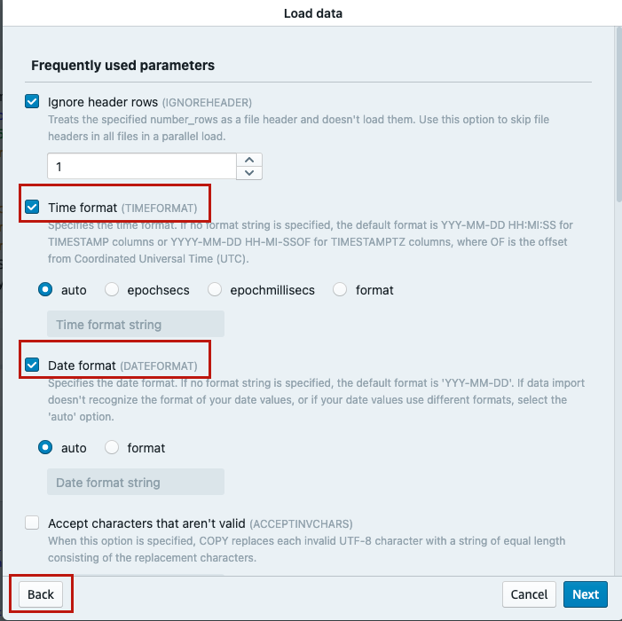

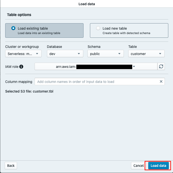


 Erol Murtezaoglu, a Technical Product Manager at AWS, is an inquisitive and enthusiastic thinker with a drive for self-improvement and learning. He has a strong and proven technical background in software development and architecture, balanced with a drive to deliver commercially successful products. Erol highly values the process of understanding customer needs and problems, in order to deliver solutions that exceed expectations.
 Sapna Maheshwari is a Sr. Solutions Architect at Amazon Web Services. She has over 18 years of experience in data and analytics. She is passionate about telling stories with data and enjoys creating engaging visuals to unearth actionable insights.
 Karthik Ramanathan is a Software Engineer with Amazon Redshift and is based in San Francisco. He brings close to two decades of development experience across the networking, data storage and IoT verticals. When not at work he is also a writer and loves to be in the water.
 Albert Harkema is a Software Development Engineer at AWS. He is known for his curiosity and deep-seated desire to understand the inner workings of complex systems. His inquisitive nature drives him to develop software solutions that make life easier for others. Albert’s approach to problem-solving emphasizes efficiency, reliability, and long-term stability, ensuring that his work has a tangible impact. Through his professional experiences, he has discovered the potential of technology to improve everyday life.


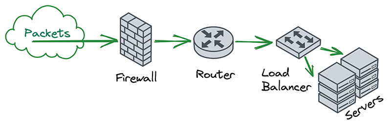
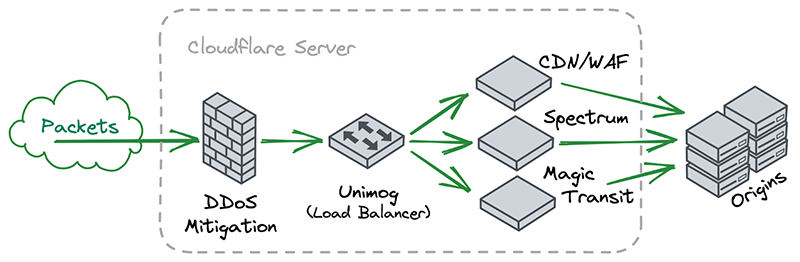
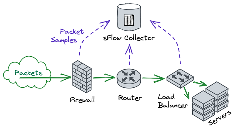
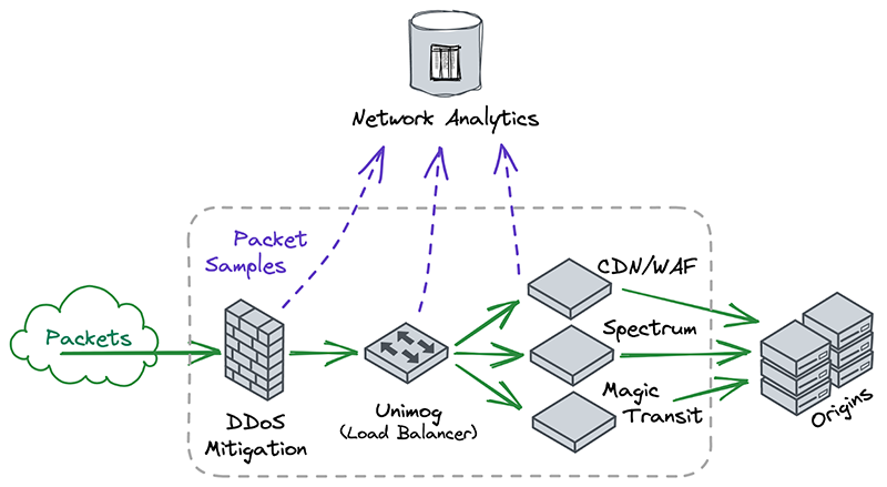
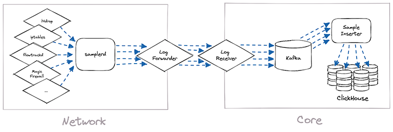
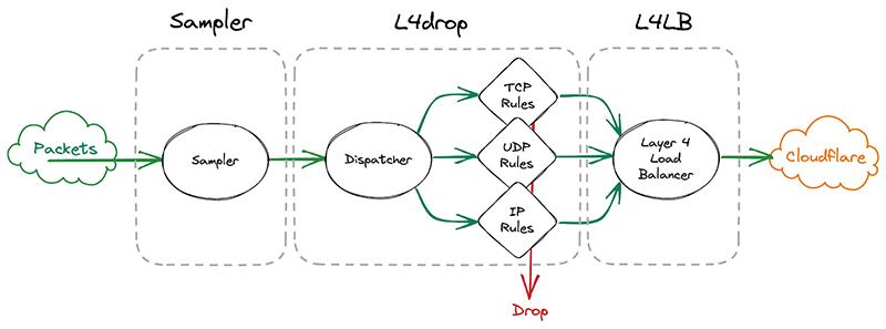
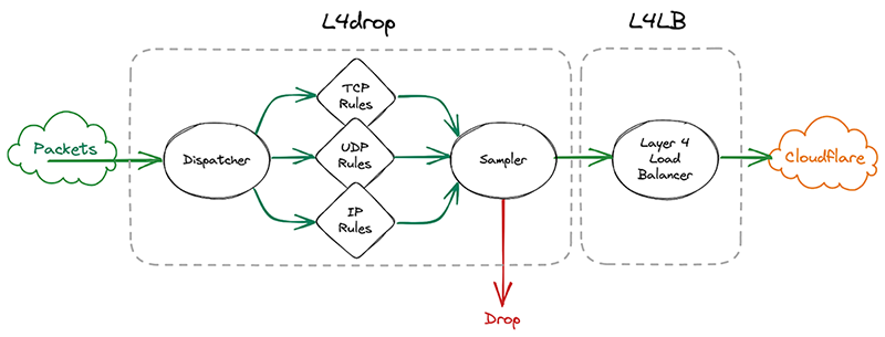


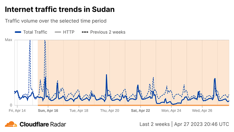
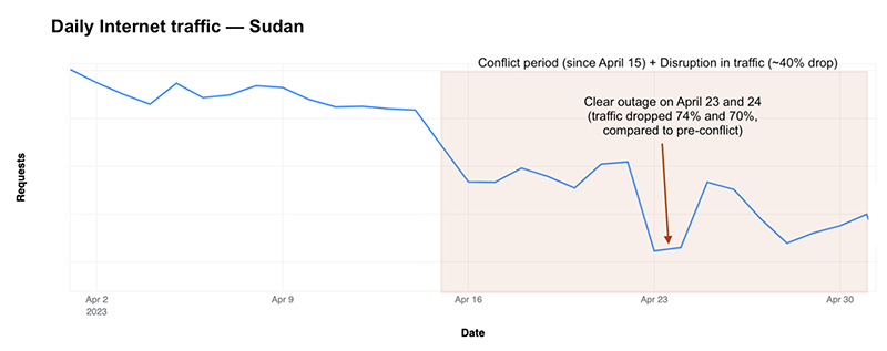
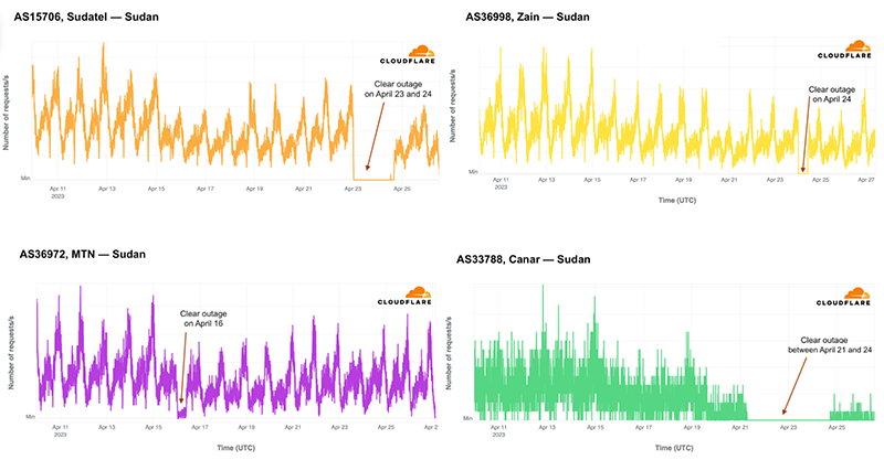
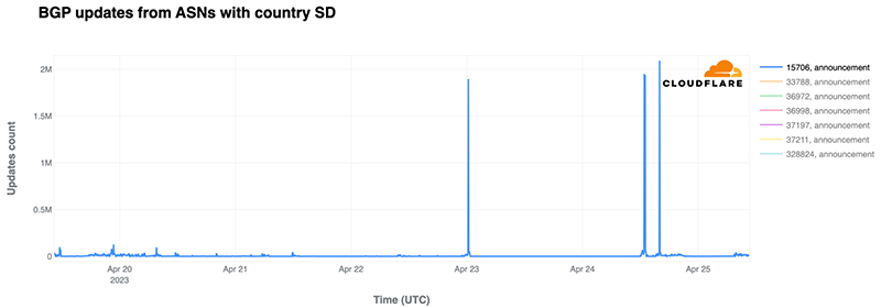
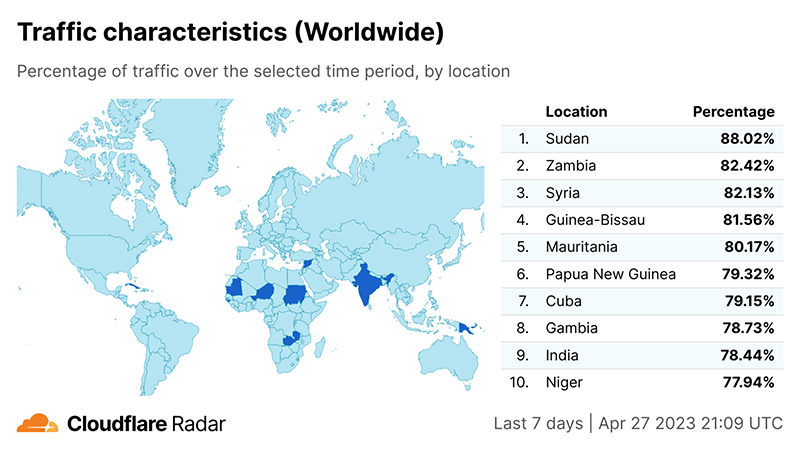
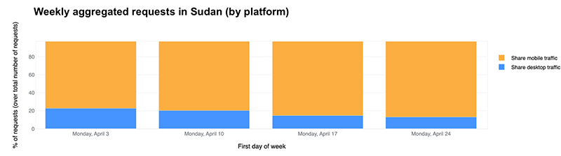
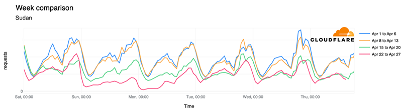
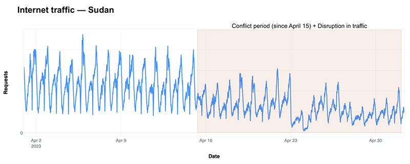
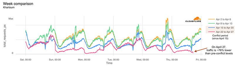
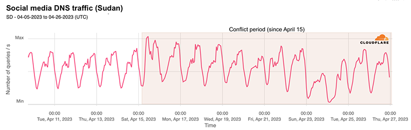

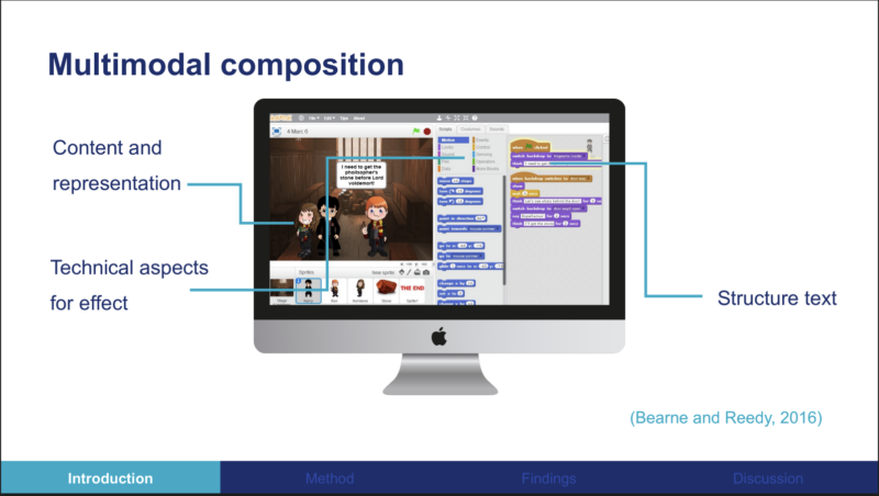
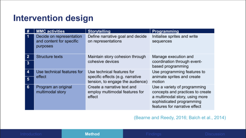
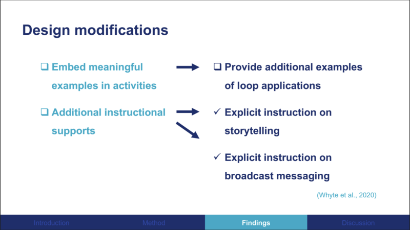


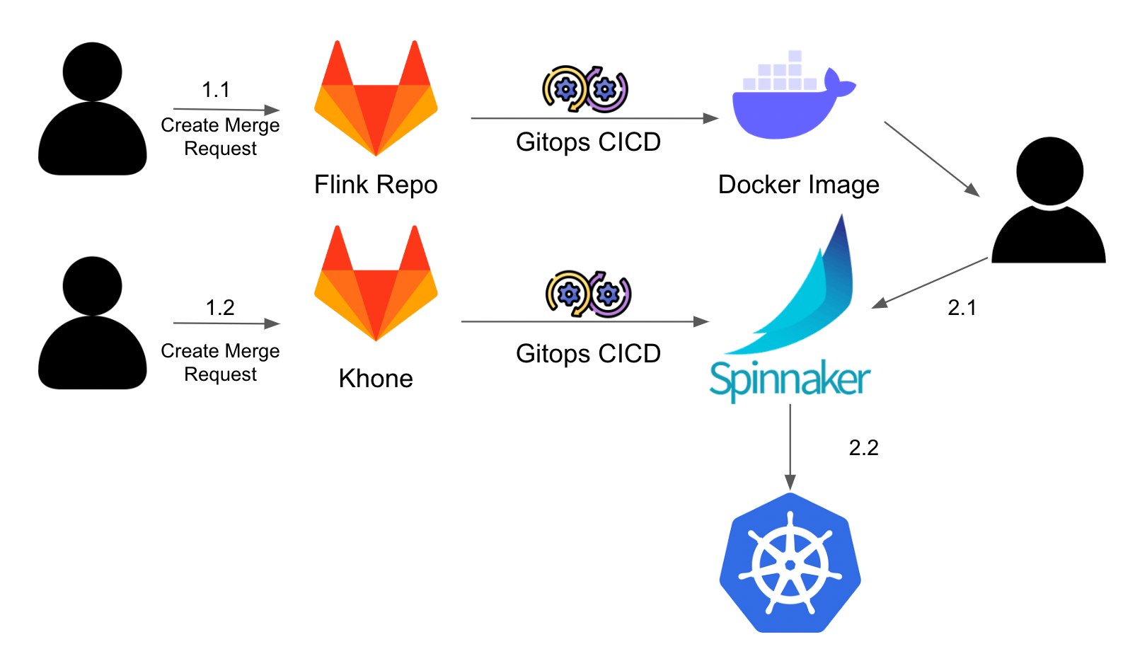
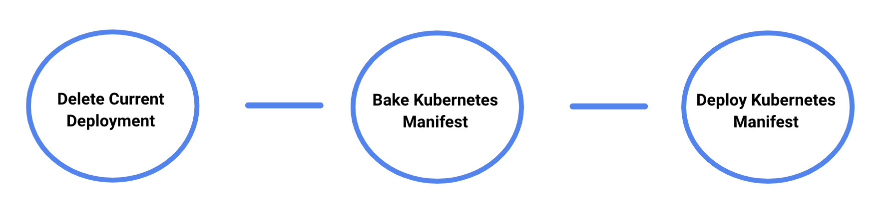

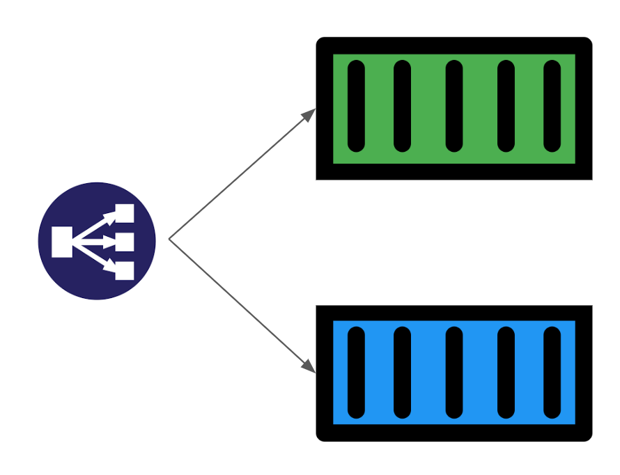
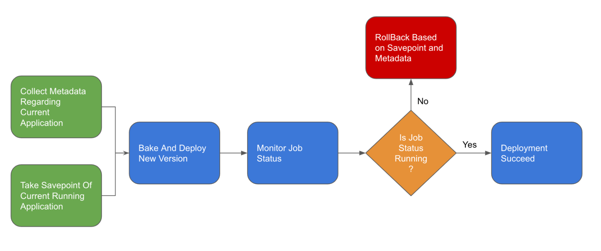
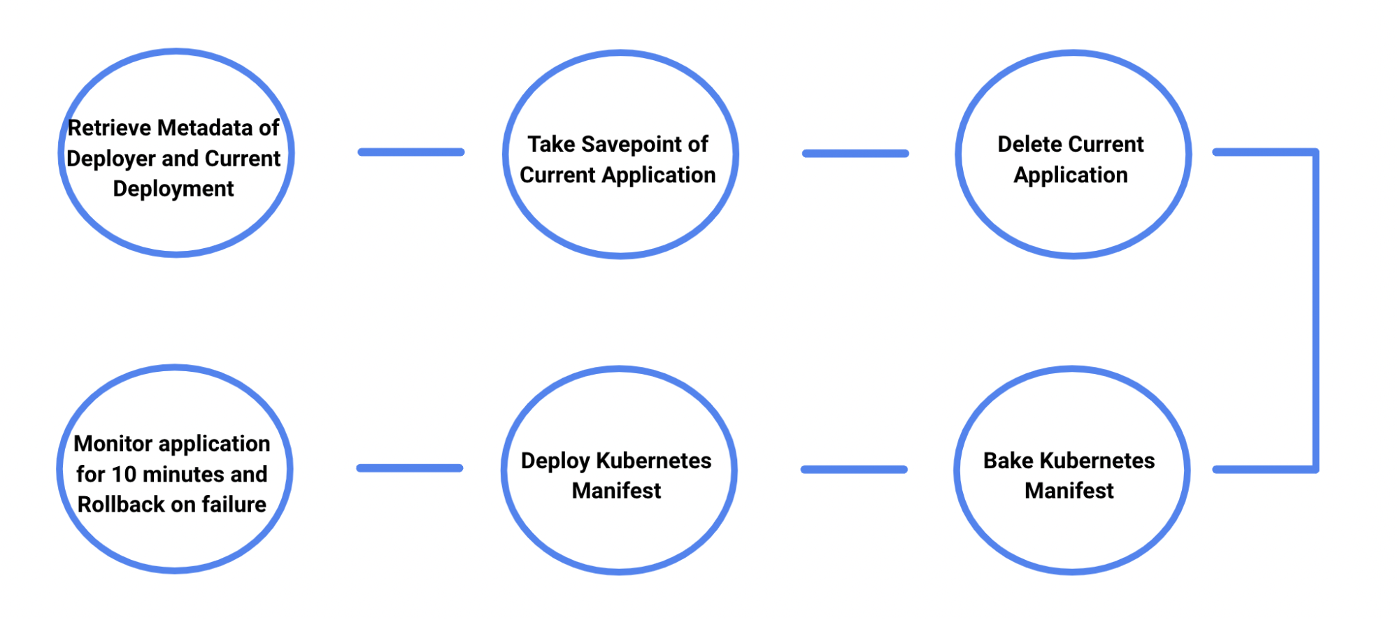
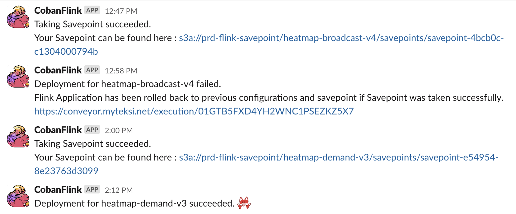
 AWS Global Summits – Check your calendars and sign up for the AWS Summit close to where you live or work: