За блогърстването и още нещо

Post Syndicated from Йовко Ламбрев original https://blog.yovko.net/za-blogarstvaneto/

Този текст е провокиран от публикация на Иван, който обзет от носталгия по доброто, старо блогърстване ме сръчка да споделя и аз някакви мисли по темата. А вероятно и да имам повод напиша нещо тук. Oт последният ми пост са минали три месеца. Вероятно до края на тази особена 2020 година няма да напиша друг, но пък бих използвал време от почивните дни около Коледа да реорганизирам сайта си и своето online присъствие. За пореден път. Иначе казано, щом виждам смисъл да го правя, значи не съм се отказал окончателно.

Макар и да съзнавам напълно, че няма как да е като преди.

Интересно съвпадение е, че някъде точно по това време миналата година убих най-накрая Facebook профила си. И не просто го замразих – изтрих го. С искрена и неприкрита ненавист към тази зловеща платформа.

Разбира се, това не значи, че съм се разписал повече тук.

Блогването имаше повече стойност, когато Google Reader беше жив и беше платформа за комуникация и диалог – кой какво чете, кой какво споделя от своите прочетени неща. Днес това все още е възможно – например в Inoreader. Но вече е много по-трудно да събереш всички на едно място с подобна цел (ако не си от hi-tech гигантите), а друга е темата дали това изобщо е добра идея. Един дистрибутиран RSS-четец с подобна функционалност ще е най-доброто възможно решение.

Уви, за щастие RSS е още жив, но натискът да бъде убит този чуден протокол за споделяне на съдържание е огромен. От една страна големият враг са всички, които искат да обвързват потребители, данни и съдържание със себе си, а от друга немарливостта на web-разработчиците и дигиталните маркетолози, които проповядват, че RSS е мъртъв и не си струва усилията. Днес все по-често сайтовете са с нарочно премахнат или спрян RSS.

Без такива неща, блоговете в момента са като мегафон, на който са извадени батериите – островчета, които продължават да носят смисъл и значение, но като в легендата за хан Кубрат – няма я силата на съчките събрани в сноп.

Всъщност вината ни е обща. Защото се подхлъзваме като малки деца на шаренко по всяка заигралка в мрежата, без да оценяваме плюсовете и минусите, още по-малко щетите, които би могла да нанесе. Интернет вече е платформа с по-голямо социално, отколкото технологично значение – оценка на въздействието би трябвало да бъде задължителна стъпка в тестването на всяка нова идея или проект в мрежата. И то не толкова от този, който я пуска, защото обикновено авторът е заслепен от мечти и жажда за слава (а често и неприкрита алчност), а от първите, че и последващите потребители.

Блогърите предадохме блогването, защото „глей к’во е яко да се пра’иш на интересен в 140 знака в твитър“ или „как ши стана мега-хипер-секси инфлуенцър с facebook и instagram в три куци стъпки“. Нищо, че социалките може и да те усилват (до едно време), но после само ти крадат трафика. И се превърщат в посредник със съмнителна добавена стойност, но пък взимащ задължително своето си.

Това всъщност беше само върхът на айсберга, защото от самото начало технооптимизмът беше в повече. В много посоки и отношения. И ако това в романтичните времена на съзиданието бе оправдано, и дори полезно – сега ни е нужен технореализъм и критично отношение за поправим счупеното.

Интернет днес не е това, което трябваше да бъде. Гравитацията на гигантите засмука всичко. И продължава. И ако не искаме да се озовем в черна дупка са нужни общи усилия за децентрализирането му. Това няма да е лесно, защото този път създателите няма да имат много съюзници от страна на бизнеса. Предстои трудна война с гигантите и влиянието им. Единственият могъщ съюзник сме си ние хората, ако успеем да си обясним помежду си защо е нужно да се съпротивляваме.

Засега не успяваме.

P.S. Т.е. псст, подхвърлям топката към Ясен и Мария.

Personal Raspberry Pi music streamer

Post Syndicated from Ashley Whittaker original https://www.raspberrypi.org/blog/personal-raspberry-pi-music-streamer/

Mike Perez from Audio Arkitekts took to YouTube to show you how to build your own music streamer using a Raspberry Pi. Haters of Bluetooth and RCA plugs, he’s done this for you.

Mike reports a “substantial difference in sound quality” compared to his previous setup (the aforementioned and reviled Bluetooth and RCA plug options).

This project lets you use a Raspberry Pi as a music player and control it from your mobile phone.

Hardware

Unboxing the Argon Neo Raspberry Pi Bundle

Mike started out with an $80 Argon Neo Raspberry Pi Bundle, which includes a Raspberry Pi 4 Model B. He made a separate video to show you how to put everything together.

This bundle comes with a nice, sleek case, so your music player can be on display discreetly.

Pretty case

Not sure about spending $80 on this kit? In the project video, Mike says it’s “totally, totally worth it” — partly due to the quality of the case.

Software

Mike grabbed a compatible Volumio image from Volumio’s ‘Get Started’ page and flashed it onto Raspberry Pi with Etcher.

Volumio app in action

You can use an Ethernet cable, but Mike wanted to utilise Raspberry Pi 4’s wireless connectivity to boot the Volumio app. This way, the Raspberry Pi music player can be used anywhere in the house, as it’ll create its own wireless hotspot within your home network called ‘Volumio’.

Eew! No more direct audio connection to your phone to listen to music.

You’ll need a different version of the Volumio app depending on whether you have an Android phone or iPhone. Mike touts the app as “super easy, really robust”. You just select the music app you usually use from the ‘Plugins’ section of the Volumio app, and all your music, playlists, and cover art will be there ready for you once downloaded.

And that’s basically it. Just connect to the Volumio OS via the app and tell your Raspberry Pi what to play.

Amp it up

To get his new music player booming all around the house, Mike used a Starke Sound AD4, which you can watch him unbox and review.

What kind of amplification system have you got paired up with your Raspberry Pi–powered music player?

The post Personal Raspberry Pi music streamer appeared first on Raspberry Pi.

New – Attributes Based Access Control with AWS Single Sign On

Post Syndicated from Sébastien Stormacq original https://aws.amazon.com/blogs/aws/new-attributes-based-access-control-with-aws-single-sign-on/

Starting today, you can pass user attributes in the AWS session when your workforce sign-in into the cloud using AWS Single Sign-On. This gives you the centralized account access management of AWS Single Sign-On and ABAC, with the flexibility to use AWS SSO, Active Directory, or an external identity provider as your identity source. To learn more about the advantages of ABAC policies on AWS, you may read my previous blog post on the subject.

Overview
On one side, system administrators configure user attributes on the AWS Single Sign-On identity repository, or the managed Active Directory. System administrators may also configure an external identity provider, such as Okta, OneLogin or PingFederate to pass existing user attributes in the AWS sessions when their workforce federates into AWS. These attributes are known as session tags in AWS. On the other side, cloud administrators create fine-grained permissions policies such that your workforce get only access to cloud resources with matching resource tags.

Creating policies based on matching attributes instead of functional roles helps to reduce the number of distinct permissions and roles you must create and manage in your AWS environment. For example, when developers Bob from team red and Alice from team blue sign-in into AWS and assume the same AWS Identity and Access Management (IAM) role, they get distinct permissions to project resources tagged for their team. The identity system sends the team name attribute in the AWS session when Bob and Alice sign-in into AWS. The role’s permissions grant access to project resources with matching team name tags. Now, if Bob moves to team blue and system administrators update his team name in their identity provider directory, Bob automatically gets access to team blue’s project resources without requiring permissions updates in IAM.

How to Configure AWS SSO to Map User Attributes
Before to configure AWS SSO, there are two important points to highlight. First, ABAC will work with attributes from any identity source configured in AWS SSO : AWS SSO itself, a managed Active Directory, or an external identity provider. Second, there are two ways to pass attributes for access control to AWS SSO. Either you can pass attributes directly in the SAML assertion using the prefix https://aws.amazon.com/SAML/Attributes/AccessControl, or you can use attributes that are in the AWS SSO identity store. Those attributes are configured by your AWS SSO administrator for users created in AWS SSO, synchronized in from an Active Directory, or synchronized in from an external identity provider using automatic provisioning (SCIM).

For this demo, I choose to use an external identity provider and SCIM.

I can enable ABAC in AWS using AWS SSO with three steps:

Step 1: I configure my identity source with the associated user identities and attributes in the external identity provider. As of today, AWS SSO supports identity synchronization via SCIM with Azure AD, Okta, OneLogin, and PingFederate. Check this page to get an up-to-date list. The specifics depend on each identity provider.

Step 2: I configure the SCIM attributes I want to use for access control using the new Access Control Attributes global setting in the AWS SSO console or API. This screen allows me to select attributes for access control from the identity source I configured in step 1.

Attributes for Access Control

Step 3: I author ABAC rules through permission sets and resource-based policies using the attributes I configured in Step 2. More about this in a minute.

Now, when my workforce federates into an AWS account using SSO, they get access to their AWS resources based on matching attributes.

Attributes are passed as session tags. They are passed as comma-separated key:value pairs. The total character length of all the attributes together must be less than or equal to 460 characters.

What Does a Policy Look Like?
I now can use user attributes in my permission sets using the aws:PrincipalTag condition key when creating access control rules. For example, I can tag all the resources in my organization with their respective department name, and use a single permission set that grants developers access only to their department resources. Now, whenever developers federate into the AWS account, AWS SSO creates a department session tag with the value received from the identity provider. The security policies allow them to only get access to the resources in their respective department. As the team adds more developers and resources to their project, I only have to tag resources with the correct department name. As a result, as the organization adds new resources and developers to departments, developers can only manage resources aligned to their department without needing any permission updates.

An ABAC SSO permission set policy might look like this:

{
    "Version": "2012-10-17",
    "Statement": [
        {
            "Effect": "Allow",
            "Action": [ "ec2:DescribeInstances"],
            "Resource": "*"
        },
        {
            "Effect": "Allow",
            "Action": ["ec2:StartInstances","ec2:StopInstances"],
            "Resource": "*",
            "Condition": {
                "StringEquals": {
                    "ec2:ResourceTag/Department": "${aws:PrincipalTag/Department}"
                }
            }
        }
    ]
}

This policy allows anybody to DescribeInstances, but only users with a aws:PrincipalTag/Department tag’s value matching the EC2 instance ec2:ResourceTag/Department tag’s value are authorized to stop or to start instances.

I attach this policy to an AWS Account’s Permission Set. On the left part of the AWS Single Sign-On console, I click AWS Accounts and select the Permission sets tab. Then I click Create permission set. On the next screen, I select Create a customer permission set.

Create a custom permission set

I enter a name and description, I make sure Create a custom permissions policy is selected. Then I can copy/paste the previous policy allowing to start and stop EC2 instances when the department name tag value is equal to the person’s department name tag value.

Create Custom Policy for Permission Set

On the next screen, I enter some tags, then I review my configuration before clicking Create. Et voila, I am ready to go.

If you have existing federation configured with AWS Security Token Service, remember that external identity providers consider AWS SSO as a new application configuration. This means when you move from direct IAM federation to AWS SSO, you have to update your external identity provider configuration to connect with AWS SSO and to introduce attributes as session tags for this configuration.

Available Today
There is no additional charge to configure user attributes with AWS Single Sign-On. You can start to use it today in all AWS Regions where AWS SSO is available.

— seb

An API is a user interface

Post Syndicated from arp242.net original https://www.arp242.net/api-ux.html

An API is a user interface for programmers and is essentially no different from
a graphical user interface, command-line user interface, or any other interface
a human (“user”) is expected to work with. Whenever you create a publicly
callable function you’re creating a user interface. Programmers are users, too.

This applies for any API: libX11, libpng, Ruby on Rails (good UX is a major
factor for Rails’ success), a REST API, etc.

A library exists of two parts: implementation and exposed API. The
implementation is all about doing stuff and interacting with the computer,
whereas the exposed API is about giving a human access to this, preferably in a
convenient way that makes it easy to understand, and making it hard to get
things wrong.

This may sound rather obvious, but in my experience this often seems forgotten.
The world is full of badly documented clunky APIs that give confusing errors (or
no errors!) to prove it.

Whenever I design a public package, module, or class I tend to start by writing
a few basic usage examples and documenting it. This first draft won’t be perfect
and while writing the implementation I keep updating the examples and
documentation to iterate on what works and axe what doesn’t. This is kind of
like TDD, except that it “tests” the UX rather than the implementation. Call it
Example Driven Development if you will.

This is similar to sketching a basic mock UI for a GUI and avoids “oh, we need
to be able to do that too” half-way through building your UI, leading to awkward
clunky UI elements added willy-nilly as an afterthought.

In code reviews the first questions I usually have are things like “is this API
easy to use?”, “Is it consistent?”, “can we extend it in the future so it won’t
be ugly?”, “is it documented, and is the documentation comprehensible?”.
Sometimes I’ll even go as far as trying to write a simple example to see if
there are any problems and if it “feels” right. Only if this part is settled do
I move on to reviewing the correctness of the actual implementation.


I’m not going to list specific examples or tips here; it really depends on the
environment, intended audience (kernel programmers are not Rails programmers),
and most of all: what you’re doing.

Sometimes a single function with five parameters would be bad UX, whereas in
other cases it might be a good option, if all five really are mandatory for
example, or if you use Python and have named parameters. In other cases, it
makes more sense to have five functions which accepts a single parameter.

There usually isn’t “one right way”. If everyone started treating APIs as user
interfaces instead of “oh, it’s just for developers, they will figure it out”
then we’ll be 90% there.

That being said, the most useful general piece of advice I know of is John
Ousterhout’s concept of deep modules: modules that provide large functionality
with simple interfaces. Depth of module is a nice overview with goes in
to some more details about this, and I won’t repeat it here.

New Synchronous Express Workflows for AWS Step Functions

Post Syndicated from Benjamin Smith original https://aws.amazon.com/blogs/compute/new-synchronous-express-workflows-for-aws-step-functions/

Today, AWS is introducing Synchronous Express Workflows for AWS Step Functions. This is a new way to run Express Workflows to orchestrate AWS services at high-throughput.

Developers have been using asynchronous Express Workflows since December 2019 for workloads that require higher event rates and shorter durations. Customers were looking for ways to receive an immediate response from their Express Workflows without having to write additional code or introduce additional services.

What’s new?

Synchronous Express Workflows allow developers to quickly receive the workflow response without needing to poll additional services or build a custom solution. This is useful for high-volume microservice orchestration and fast compute tasks that communicate via HTTPS.

Getting started

You can build and run Synchronous Express Workflows using the AWS Management Console, the AWS Serverless Application Model (AWS SAM), the AWS Cloud Development Kit (AWS CDK), AWS CLI, or AWS CloudFormation.

To create Synchronous Express Workflows from the AWS Management Console:

  1. Navigate to the Step Functions console and choose Create State machine.
  2. Choose Author with code snippets. Choose Express.
    This generates a sample workflow definition that you can change once the workflow is created.
  3. Choose Next, then choose Create state machine. It may take a moment for the workflow to deploy.

Starting Synchronous Express Workflows

When starting an Express Workflow, a new Type parameter is required. To start a synchronous workflow from the AWS Management Console:

  1. Navigate to the Step Functions console.
  2. Choose an Express Workflow from the list.
  3. Choose Start execution.

    Here you have an option to run the Express Workflow as a synchronous or asynchronous type.
  4. Choose Synchronous and choose Start execution.

  5. Expand Details in the results message to view the output.

Monitoring, logging and tracing

Enable logging to inspect and debug Synchronous Express Workflows. All execution history is sent to CloudWatch Logs. Use the Monitoring and Logging tabs in the Step Functions console to gain visibility into Express Workflow executions.

The Monitoring tab shows six graphs with CloudWatch metrics for Execution Errors, Execution Succeeded, Execution Duration, Billed Duration, Billed Memory, and Executions Started. The Logging tab shows recent logs and the logging configuration, with a link to CloudWatch Logs.

Enable X-Ray tracing to view trace maps and timelines of the underlying components that make up a workflow. This helps to discover performance issues, detect permission problems, and track requests made to and from other AWS services.

Creating an example workflow

The following example uses Amazon API Gateway HTTP APIs to start an Express Workflow synchronously. The workflow analyses web form submissions for negative sentiment. It generates a case reference number and saves the data in an Amazon DynamoDB table. The workflow returns the case reference number and message sentiment score.

  1. The API endpoint is generated by an API Gateway HTTP APIs. A POST request is made to the API which invokes the workflow. It contains the contact form’s message body.
  2. The message sentiment is analyzed by Amazon Comprehend.
  3. The Lambda function generates a case reference number, which is recorded in the DynamoDB table.
  4. The workflow choice state branches based on the detected sentiment.
  5. If a negative sentiment is detected, a notification is sent to an administrator via Amazon Simple Email Service (SES).
  6. When the workflow completes, it returns a ticketID to API Gateway.
  7. API Gateway returns the ticketID in the API response.

The code for this application can be found in this GitHub repository. Three important files define the application and its resources:

Deploying the application

Clone the GitHub repository and deploy with the AWS SAM CLI:

$ git clone https://github.com/aws-samples/contact-form-processing-with-synchronous-express-workflows.git
$ cd contact-form-processing-with-synchronous-express-workflows 
$ sam build 
$ sam deploy -g

This deploys 12 resources, including a Synchronous Express Workflow, three Lambda functions, an API Gateway HTTP API endpoint, and all the AWS Identity & Access Management (IAM) roles and permissions required for the application to run.

Note the HTTP APIs endpoint and workflow ARN outputs.

Testing Synchronous Express Workflows:

A new StartSyncExecution AWS CLI command is used to run the synchronous Express Workflow:

aws stepfunctions start-sync-execution \
--state-machine-arn <your-workflow-arn> \
--input "{\"message\" : \"This is bad service\"}"

The response is received once the workflow completes. It contains the workflow output (sentiment and ticketid), the executionARN, and some execution metadata.

Starting the workflow from HTTP API Gateway:

The application deploys an API Gateway HTTP API, with a Step Functions integration. This is configured in the api.yaml file. It starts the state machine with the POST body provided as the input payload.

Trigger the workflow with a POST request, using the API HTTP API endpoint generated from the deploy step. Enter the following CURL command into the terminal:

curl --location --request POST '<YOUR-HTTP-API-ENDPOINT>' \
--header 'Content-Type: application/json' \
--data-raw '{"message":" This is bad service"}'

The POST request returns a 200 status response. The output field of the response contains the sentiment results (negative) and the generated ticketId (jc4t8i).

Putting it all together

You can use this application to power a web form backend to help expedite customer complaints. In the following example, a frontend application submits form data via an AJAX POST request. The application waits for the response, and presents the user with a message appropriate to the detected sentiment, and a case reference number.

If a negative sentiment is returned in the API response, the user is informed of their case number:

Setting IAM permissions

Before a user or service can start a Synchronous Express Workflow, it must be granted permission to perform the states:StartSyncExecution API operation. This is a new state-machine level permission. Existing Express Workflows can be run synchronously once the correct IAM permissions for StartSyncExecution are granted.

The example application applies this to a policy within the HttpApiRole in the AWS SAM template. This role is added to the HTTP API integration within the api.yaml file.

Conclusion

Step Functions Synchronous Express Workflows allow developers to receive a workflow response without having to poll additional services. This helps developers orchestrate microservices without needing to write additional code to handle errors, retries, and run parallel tasks. They can be invoked in response to events such as HTTP requests via API Gateway, from a parent state machine, or by calling the StartSyncExecution API action.

This feature is available in all Regions where AWS Step Functions is available. View the AWS Regions table to learn more.

For more serverless learning resources, visit Serverless Land.

A deep dive into high-cardinality anomaly detection in Elasticsearch

Post Syndicated from Kaituo Li original https://aws.amazon.com/blogs/big-data/a-deep-dive-into-high-cardinality-anomaly-detection-in-elasticsearch/

In May 2020, we announced the general availability of real-time anomaly detection for Elasticsearch. With that release we leveraged the Random Cut Forest (RCF) algorithm to identify anomalous behaviors in the multi-dimensional data streams generated by Elasticsearch queries. We focused on aggregation first, to enable our users to quickly and accurately detect anomalies in their data streams. However, consider the example data in the following table.

timestamp avg. latency region
12:00 pm 3.1 Seattle
12:00 pm 4.1 New York
12:00 pm 5.9 Berlin
12:01 pm 2.6 Seattle
12:01 pm 5.3 New York
12:01 pm 5.8 Berlin

The data consists of one data field, avg. latency, and one attribute or categorical field, time. If we want to perform anomaly detection on this data, we could take the following strategy:

  1. Separate the data by the region attribute to create a separate data stream entity for each region.
  2. Construct an anomaly detector for each entity. If the cardinality of the region attribute, that is the number of possible choices of region value, is small, we can create separate anomaly detectors by filtering on each possible value of region.

But what if the cardinality of this attribute is large? Or what if the set of possible values changes over time, such as a source IP address or product ID? The existing anomaly detection tool doesn’t scale well in this situation.

We define the high-cardinality anomaly detection (HCAD) problem as performing anomaly detection on a data stream where individual entities in the stream are defined by a choice of attribute. In this use case, our goal is to perform anomaly detection on each data stream defined by a particular choice of region. That is, the Seattle region produces its own latency data stream, as well as the New York and Berlin regions.

In this post, we dive into the motivation, design, and development of the HCAD capability. We begin with an in-depth description of the HCAD problem and its properties. We then share the details of our solution and the challenges and questions we encountered during our research and development. Finally, we describe the system and architecture of our solution, especially the components tackling scalability concerns.

High-cardinality anomaly detection

In this section, we elaborate on the definition of the HCAD problem. As described earlier, we can think of HCAD as a way to produce multiple data streams by defining each data stream by a particular choice of attribute. For each data stream, we want to perform streaming anomaly detection as usual—we want to detect anomalies relative to that individual data stream’s own history.

We define an individual entity by fixing a particular value of one or more attributes and aggregating values over all remaining attributes. In the language of table manipulation in SQL, each entity is defined using GROUPBY on an attribute. Specifically, a group of entities is defined by selecting one or more attributes, where each entity is given by the data fields for each particular value of those attributes. For example, applying GROUPBY to the region attribute in the preceding example data produces three data stream entities: one for Seattle, one for New York, and one for Berlin. Within each of these data streams, we want to find anomalies with respect to that data stream’s history.

This idea of defining a data stream entity by attribute values extends to multiple attribute fields. When multiple attribute fields exist but we group by only one of those attributes, we aggregate each entity over the remaining attribute fields. For example, suppose you have network traffic data consisting of two attribute fields and one data field. The attribute fields are a source_ip address and a dest_ip address. The data field is the number of bytes_transferred in that particular network transaction between the given two IP addresses. The following table gives an example of such a dataset.

timestamp source_ip dest_ip bytes_transferred
12:00 pm 192.168.1.1 192.168.1.20 138
12:00 pm 192.168.1.1 192.168.1.300 21
12:00 pm 192.168.1.20 192.168.1.300 5
12:01 pm 192.168.1.1 192.168.1.20 289
12:01 pm 192.168.1.1 192.168.1.300 10
12:02 pm 192.168.1.1 192.168.1.20 244
12:02 pm 192.168.1.1 192.168.1.300 16
12:02 pm 192.168.1.20 192.168.1.300 8

One way to define an entity is to group by both source IP address and destination IP address combinations. Under this method of defining entities, we end up with the following data streams.

entity: (source_ip, dest_ip) 12:00 pm 12:01 pm 12:02 pm 12:03 pm
(192.168.1.1, 192.168.1.20) 138 289 244
(192.168.1.1, 192.168.1.300) 25 10 16
(192.168.1.20, 192.168.1.300) 5 0 8

On the other hand, if we define an entity only by its source IP address, we aggregate bytes transferred over the possible destination IP addresses.

entity: (source_ip,) 12:00 pm 12:01 pm 12:02 pm 12:03 pm
(192.168.1.1,) 159 299 260
(192.168.1.20,) 5 0 8

HCAD is distinct from another anomaly detection technique called population analysis. The goal of population analysis is to discover entire entities with values and patterns distinct from other entities. For example, the bytes transferred data stream associated with the entity (192.168.1.1, 192.168.1.20) is much larger in value than either of the other entities. Assuming many entities exist with values in the range of 1 to 30, this entity is considered a population anomaly. An entity can be a population data stream contains no anomalies relative to its own history.

Depending on the way we define entities from attributes, the number of data stream entities changes. This is an important consideration with regards to scale and density of the data streams: grouping by too many attributes may leave you with entities that have too few observations for a meaningful data stream. This is not uncommon in real-world datasets. Even in a dataset with only one attribute, real-world data tends to adhere to a power-law scaling of data density. Simply put, the majority of data stream activity occurs in a minority of entities. There is likely a long tail of sparse entities. Given this observation, if the stream aggregation window is too small, there are many missing data points in these sparse entities.

Data stream models for HCAD

We described the HCAD problem, but how do we build a machine learning solution? Furthermore, how is this solution different from the currently available non-HCAD single-stream solution? In this section, we explain our process for model selection and why we arrived at using Random Cut Forests for the high-cardinality regime. We then address scalability problems by exploring RCF’s hyperparameter space. Finally, we address certain issues that arise when dealing with sparse data streams.

Model selection

Designing an HCAD solution has several scientific challenges. Whatever algorithmic solution we arrive at must satisfy several systems constraints:

  • The algorithm must work in a streaming context: aggregated feature queries are streaming in Elasticsearch and the anomaly detection models only receive each new feature aggregate one at a time
  • The HCAD solution must respect the business needs of the customer hardware and should have restricted CPU and memory impact
  • The solution should be scalable with respect to data throughput, number of entities, and number of nodes in the cluster
  • The algorithm must be unsupervised, because the goal is to classify anomalous data in a streaming context without any labeled training set

Our team identified three classes of anomaly detection model based on the relationship between number of entities and number of models:

  • 1:1 model – Each entity is given its own AD model. No data or anomaly information is shared between the models, but because the number of models scales with the number of entities, we must keep the model small to satisfy customer scaling needs.
  • N:1 model – A single AD model is responsible for detecting each entity’s anomalies. Deep learning-based AD models typically fall under this category.
  • N:K model – A subset of entities is assigned to one of several individual models. Typically, some clustering algorithm is used to determine an appropriate partition of entities by identifying common features in the data streams.

Each general class of solution has its own tradeoffs with respect to the ability to distribute across cluster nodes, scale with respect to the number of entities, and detect anomalies on benchmark datasets. After some analysis of these tradeoffs and experimentation, we decided on the 1:1 approach. Within this class of HCAD solution, there are many candidate data stream anomaly detection algorithms. We explored many of these algorithms and tested different lightweight models before deciding on using Random Cut Forests. RCF works particularly well across a wide variety of data stream behaviors. This fit well with our goal of providing support for as wide of a range of customer use cases as possible.

Scaling Random Cut Forests

To keep memory costs down when using RCFs as our AD model, we started by exploring the algorithm’s hyperparameter space. The model has three main hyperparameters:

  • T – Number of trees
  • S – Sample size per free
  • D – Shingle dimension

The RCF model size is O(TDS). Sample size per tree is related to expected anomaly rate, and based on our experiments with a wide variety of datasets, it was best to leave this hyperparameter at its default value of 256 from the single-stream solution. The dimensionality is a function of the customer input but also of the model’s shingle size. We discuss the role of shingle size in the next section. Primarily to satisfy the scaling and model size constraints of the HCAD system, we focused on studying the effect of the number of trees on algorithm performance.

Experiments show that 10 trees per forest gives acceptable results on benchmark datasets; a default number of 100 trees is used in the single-stream solution. In the original plugin, we chose this large number of trees to ensure that the model can keep an accurate sketch of a long enough period of data samples. In doing so, we can recognize long time-scale changes to the data stream. However, we found in our benchmark high-cardinality data streams that this large of a model is unnecessary and that 10 trees is often sufficient for summarizing each high-cardinality data stream’s statistics.

Our experiments measured the precision and recall on labeled data streams. Labels were of the form of anomaly windows: regions in time where an anomaly is known to occur at some point inside the window. A true positive is the positive identification of such a window by the anomaly detection method. Any positively predicted point outside a window is considered a false positive. For an example labeled dataset, see Using Random Cut Forests for real-time anomaly detection in Amazon Elasticsearch Service.

Handling sparse data streams

As mentioned earlier, real-world high-cardinality datasets typically exhibit a power-law like distribution in entity activity. That is, a minority of the entities produce the majority of the data. The earlier source and destination IP address use case is an example: for many websites, the majority of traffic comes from a small collection of sources, whereas individual visitors make up a long tail of sparse activity. Under this assumption, the choice of shingle size is important in defining our entity data streams.

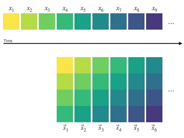
Shingling is a standard preprocessing technique for transforming a one-dimensional data stream xt​ into a d-dimensional data stream st​ by converting subsequences of length d into d-dimensional vectors: st = (xt−d+1​, …, xt−1​, xt​). The following diagram illustrates the shingling process using a shingle size of four.

These vectors, instead of the raw stream values, are then fed into the RCF model. In anomaly detection, using shingling has several benefits. First, shingling filters out small-scale noise in the data. Second, shingles allow the model to detect breaks in certain local patterns or frequency changes. That is, a shingled RCF model learns some of the local temporal behavior of your data stream.

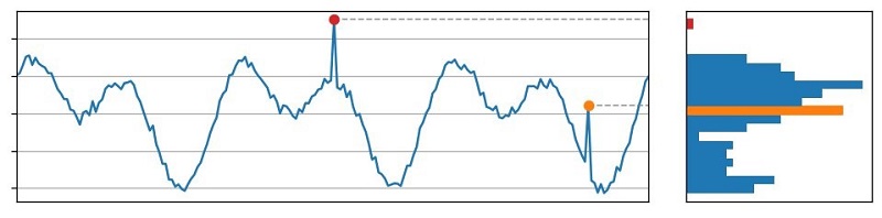
From discussions with our customers and analysis of real-world anomalies, we realized that many customers are looking for distributional anomalies: values that are outside the normal range of values of a data stream. This is in contrast to contextual anomalies, where a data point is considered anomalous in the context of just the data stream’s local history. The following figure depicts this distinction. On the left is a plot of a data stream, and on the right is a histogram of the values attained by this stream in the time window shown. The red data point is a distributional anomaly because its value falls within a low-density regime of the value distribution. The orange data point, on the other hand, is a contextual anomaly: its value is commonly occurring within this span of time but the presence of a spike at this particular point in time is unexpected.

The use of a shingle dimension greater than one allows the RCF model to detect these contextual anomalies in addition to the distributional anomalies.

One challenge with using shingles, however, is how to handle missing data. When data is unavailable at a particular time t, the shingles at times t, t+1, …, t+d−1 cannot be constructed. This results in a delay in the model’s ability to report anomalies. Our the impact of the occasional missing datum by using interpolation. However, when a data stream is sparse, it’s unlikely that any shingle can be constructed, thus turning interpolation into a prediction problem. Whether or not shingling is appropriate for your data is a function of the aggregation window used in the Elasticsearch query and the entity data density.

Scaling anomaly detection in Elasticsearch

In this section, we deep dive into the engineering challenges encountered in building the HCAD tool, particularly regarding the scalability with respect to the number of entities. We first describe the challenges we faced. Then we explain how our HCAD solution balances scalability and resource usage. Finally, we collected these ideas into a description of the overall HCAD framework.

The challenge

As described earlier, our goal was to support filtering the data by attribute or categorical fields and create a separate model for each attribute or categorical value. After examining several real-world use cases, we needed the HCAD plugin to handle millions of categorical values. Processing this many unique values was a challenging scalability issue that affected several key resources:

  • Storage – At the extreme, with 100 1-minute interval detectors and millions of entities for each detector running on our evaluation workload, we have seen the checkpoint index reach up to 170 GB in 1 day.
  • Memory – Compared to the single-stream detector, we could decrease the model size by approximately 20 times by decreasing shingle size and the number of RCF trees. But the number of entities is unbounded.
  • CPU – A single-stream detector mostly runs serial processing. During an HC detector run, multiple entities compete for CPU cycles for model update and inference. The CPU time grows linearly relative to the number of entities processed in each AD job run.

Designing for scalability and resource control

Based on these scalability issues, we chose to extend the current AD architecture because it already had these attributes:

  • Easy to scale out
  • Powerful enough to handle unpredictable scaling requirements
  • Able to control resource usage

However, meeting these challenges for HCAD required three key changes to our existing AD architecture.

First, we placed embarrassingly parallel computations on multiple nodes instead of a coordinating node. The coordinating node acts as the start of the task workflow. It only fetches features and assigns each node in the cluster a portion of the features that is roughly the same in size for all nodes. Other nodes process the features, train and run local models, and write results. Therefore, increasing the number of nodes by a factor of K asymptotically increases the number of categorical values we can handle by the same factor.

Second, in a single-stream detector, the amount of memory used is proportional to the number of features and is fixed when the detector is defined. However, with the introduction of HCAD, the number of entities is not fixed and the number of active entities is likely to change. Therefore, the size of the required memory may continuously change in the lifetime of a detector. Caching can accommodate such requirements without the need to pre-allocate memory for a detector in a fixed amount. If enough memory exists, we create models for all entities and monitor anomalies. Otherwise, we cache the hottest entities’ models up to the amount that the cache memory can contain. For example, if our memory can host only 100 models and there are millions of entities, the maximum active entities in the cache are the hottest 100 entities. We maintain a time-decayed count of each entity. The cache uses this information to measure an entity’s hotness.

Finally, we implemented various strategies for combating the extra overhead of running HC detectors:

  • Rate limiting – We limit concurrent computations and throttle bursty usage. For example, when replacing models in the cache, the cache sends get and search requests to fetch and potentially train models. If there is bursty traffic to replace models, the number of requests might exceed Elasticsearch’s get and search thread pool’s maximum queue size and cause Elasticsearch to reject all get and search requests. We install rate limiting to restrict models’ replacing speed.
  • Active cleanup – This keeps resource usage under a safe level before it’s too late. For example, we keep checkpoints within 3 days. When any of the checkpoint shards is larger than 50 GB (recommended maximum shard size), we start deleting checkpoints more aggressively.
  • Minimizing space usage – For example, in single-stream anomaly detection, we record a model’s running results during each interval. An entity’s model may take time to get ready when there is not enough historical data for training. We don’t need to record such entities’ results because we won’t record anything useful other than that anomaly grade and confidence are both equal to zero. This optimization can reduce the result index size by 4–8 times in one of our experiments.

Architecture

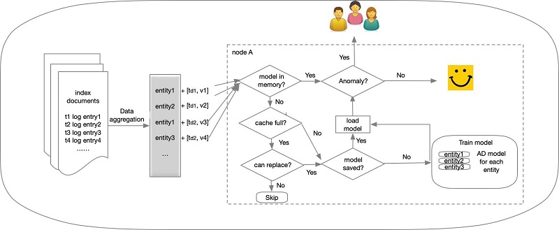
The following figure summarizes the HCAD architecture.

The end-to-end story of HCAD is as follows:

  1. A user wants to get alerts when an anomaly for a particular entity in the whole corpus arises (for example, high CPU usage on a host).
  2. The user creates an HCAD detector to describe the source data (index name), feature (for example, average CPU usage within an interval), and sampling frequency (for example, 1 minute).
  3. Based on the detector configuration, the AD plugin issues a query to fetch feature data for each host regularly (every 1 minute). Users don’t need to know what hosts to query for in the first place.
  4. A coordinating node infers the entities from the query result.
  5. The coordinating node distributes entities’ features to all nodes in the cluster.
  6. On each node, models are trained for the incoming entities, and anomaly grades are inferred, indicating how different the current CPU usage is from the trends that have recently been observed for the same hosts’ CPU usage.
  7. If cache memory is enough for all incoming entities, the cache admits entities’ models based on the entities’ hotness.

The Kibana workflow

In this section, we show how to use the HCAD in Kibana. Let’s imagine that we need to monitor the high or low CPU usage of our hosts. To do that, we create a detector, define its features, and choose a category field.

Creating a detector

To create and configure a detector, complete the following steps:

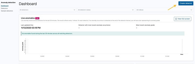
  1. On the navigation bar, choose Anomaly detection.
  2. Choose Create detector.

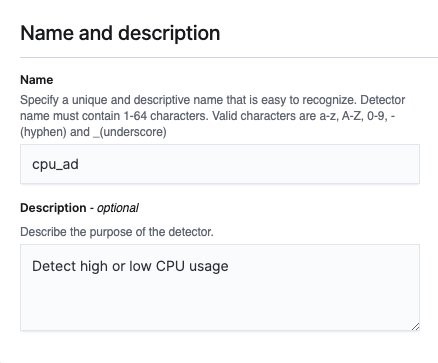
  1. Enter a name and description for the detector.

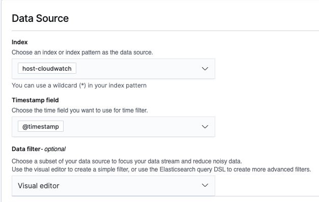
  1. Choose index or enter index pattern for the data source.
  2. For Timestamp field, choose a field so the detector can create a time series profile of the data.
  3. If you want the detector to ignore specific data (such as invalid CPU usage number), you can configure a data filter.

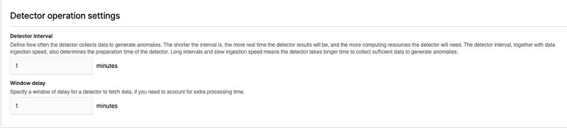
  1. Specify time frames for detection interval and window delay.

Window delay time should be a conservative estimate. Otherwise, the detector may query for documents within an interval that has not been indexed yet. For this post, we want to have an average CPU usage per minute, and we expect the index processing time to be 1 minute at most.

Defining features

In addition to the preceding settings, we need to add features. The detector aggregates a set of values within a time interval (shingle) to compute the single value according to the feature definition.

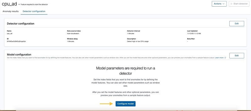
  1. Choose Configure model.

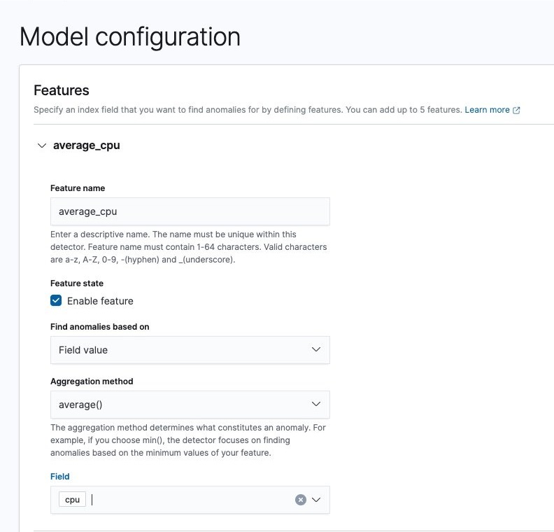
  1. For Feature name, enter a name.
  2. Specify your aggregation functions and fields.

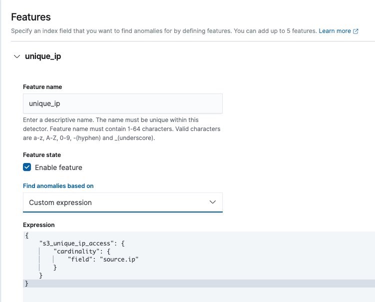
We provide five built-in single metric aggregations: Min, Max, Sum, Average, and Count. You can add a customized aggregation by choosing Custom expression for Find anomalies based on. For this post, we add a feature that returns the average of CPU usage values.

As mentioned earlier, you can customize the aggregation method as long as it returns a single value. For example, when a DevOps engineer wants to monitor the count of distinct IPs accessing their company’s Amazon Simple Storage Service (Amazon S3) buckets, they can define a cardinality aggregation that counts unique source IPs.

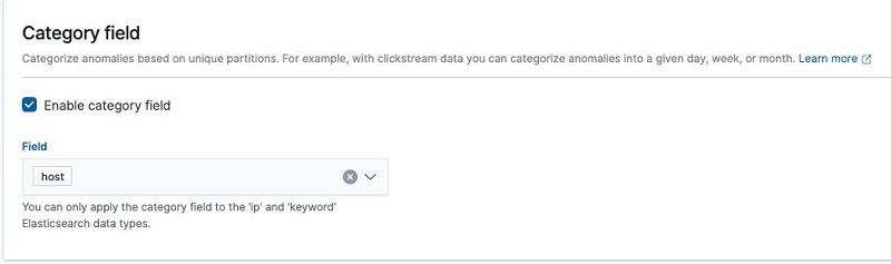
Choosing a category field

The host-cloudwatch index in our example has CPU usage per host per minute. We can define a single-stream detector to model all of the hosts’ average CPU usage together. But if each host’s CPU values have different distributions, we can split the hosts’ time series and model them separately. Giving each categorical value a separate baseline is the main change that HCAD introduces.

Previewing and starting the detector

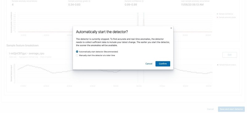
You might want to try out different choices of detector configurations and feature definitions before finalizing them. You can use Sample anomalies for iterative experiments.

Start the detector by choosing  Save and start detector. After confirming, the anomaly detector starts collecting data in real time and performing detection.

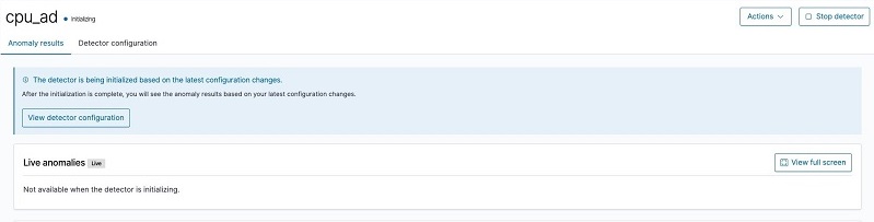
The detector starts in an initializing state.

We can use the profile API to check initialization progress (see the following code). A detector is initialized if its hottest entities’ models are fully initialized and ready to emit anomaly grade. Because the hottest entity may change, the initialization progress may go backward.

GET _opendistro/_anomaly_detection/detectors/stf6vnUB0XEggmgl3TCj/_profile/init_progress

{
    "init_progress": {
        "percentage": "92%",
        "estimated_minutes_left": 10,
        "needed_shingles": 10
    }
}

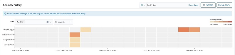
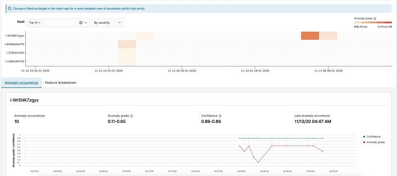
After the detector runs for a while, we can check its result on the detector’s Anomaly results tab. The following heatmap gives an overview of anomalies per entity across a timeline, by showing the hostname along the Y-axis and the timeline along the X-axis. A colored block means there is an anomaly, and a gray block means there is no anomaly.

Choosing one of the blocks shows you a more detailed view of the anomaly grade and confidence and the feature values causing the anomalies. We can observe the detector reports anomalies between 4:30 and 4:50 because the CPU usage is approaching 100%.

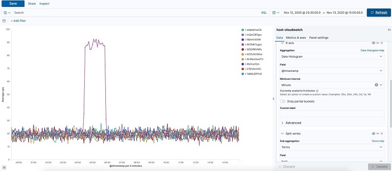
The time series of the host-cloudwatch index confirms host i-WrSNK7zgys has a CPU usage spike between 4:30–4:50.

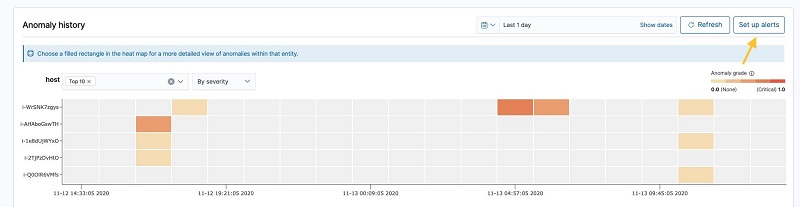
We can set up alerts for the detection results. For instructions, see Anomaly Detection.

Conclusion

General-purpose anomaly detection is challenging. Earlier in 2020, we launched a tool that can find anomalies in your feature queries. In this work, we extended the anomaly detection capabilities to the high-cardinality case. We can now find anomalies within your data when the data contains attribute or categorical fields. Our solution can discover anomalies across many entities defined by these attribute values and also scale with respect to increasing or decreasing number of entities in your data. We look forward to hearing your questions, comments, and feedback.


About the Authors

Kaituo Li is an engineer in Amazon Elasticsearch Service. He has worked on distributed systems, applied machine learning, monitoring, and database storage in Amazon. Before Amazon, Kaituo was a PhD student in Computer Science at the University of Massachusetts Amherst. He likes reading, watching TV, and sports.


Chris Swierczewski is an applied scientist at AWS. He enjoys reading, weightlifting, painting, and board games.

Introducing Amazon Managed Workflows for Apache Airflow (MWAA)

Post Syndicated from Danilo Poccia original https://aws.amazon.com/blogs/aws/introducing-amazon-managed-workflows-for-apache-airflow-mwaa/

As the volume and complexity of your data processing pipelines increase, you can simplify the overall process by decomposing it into a series of smaller tasks and coordinate the execution of these tasks as part of a workflow. To do so, many developers and data engineers use Apache Airflow, a platform created by the community to programmatically author, schedule, and monitor workflows. With Airflow you can manage workflows as scripts, monitor them via the user interface (UI), and extend their functionality through a set of powerful plugins. However, manually installing, maintaining, and scaling Airflow, and at the same time handling security, authentication, and authorization for its users takes much of the time you’d rather use to focus on solving actual business problems.

For these reasons, I am happy to announce the availability of Amazon Managed Workflows for Apache Airflow (MWAA), a fully managed service that makes it easy to run open-source versions of Apache Airflow on AWS, and to build workflows to execute your extract-transform-load (ETL) jobs and data pipelines.

Airflow workflows retrieve input from sources like Amazon Simple Storage Service (S3) using Amazon Athena queries, perform transformations on Amazon EMR clusters, and can use the resulting data to train machine learning models on Amazon SageMaker. Workflows in Airflow are authored as Directed Acyclic Graphs (DAGs) using the Python programming language.

A key benefit of Airflow is its open extensibility through plugins which allows you to create tasks that interact with AWS or on-premise resources required for your workflows including AWS Batch, Amazon CloudWatch, Amazon DynamoDB, AWS DataSync, Amazon ECS and AWS Fargate, Amazon Elastic Kubernetes Service (EKS), Amazon Kinesis Firehose, AWS Glue, AWS Lambda, Amazon Redshift, Amazon Simple Queue Service (SQS), and Amazon Simple Notification Service (SNS).

To improve observability, Airflow metrics can be published as CloudWatch Metrics, and logs can be sent to CloudWatch Logs. Amazon MWAA provides automatic minor version upgrades and patches by default, with an option to designate a maintenance window in which these upgrades are performed.

You can use Amazon MWAA with these three steps:

  1. Create an environment – Each environment contains your Airflow cluster, including your scheduler, workers, and web server.
  2. Upload your DAGs and plugins to S3 – Amazon MWAA loads the code into Airflow automatically.
  3. Run your DAGs in Airflow – Run your DAGs from the Airflow UI or command line interface (CLI) and monitor your environment with CloudWatch.

Let’s see how this works in practice!

How to Create an Airflow Environment Using Amazon MWAA
In the Amazon MWAA console, I click on Create environment. I give the environment a name and select the Airflow version to use.

Then, I select the S3 bucket and the folder to load my DAG code. The bucket name must start with airflow-.

Optionally, I can specify a plugins file and a requirements file:

  • The plugins file is a ZIP file containing the plugins used by my DAGs.
  • The requirements file describes the Python dependencies to run my DAGs.

For plugins and requirements, I can select the S3 object version to use. In case the plugins or the requirements I use create a non-recoverable error in my environment, Amazon MWAA will automatically roll back to the previous working version.


I click Next to configure the advanced settings, starting with networking. Each environment runs in a Amazon Virtual Private Cloud using private subnets in two availability zones. Web server access to the Airflow UI is always protected by a secure login using AWS Identity and Access Management (IAM). However, you can choose to have web server access on a public network so that you can login over the Internet, or on a private network in your VPC. For simplicity, I select a Public network. I let Amazon MWAA create a new security group with the correct inbound and outbound rules. Optionally, I can add one or more existing security groups to fine-tune control of inbound and outbound traffic for your environment.

Now, I configure my environment class. Each environment includes a scheduler, a web server, and a worker. Workers automatically scale up and down according to my workload. We provide you a suggestion on which class to use based on the number of DAGs, but you can monitor the load on your environment and modify its class at any time.

Encryption is always enabled for data at rest, and while I can select a customized key managed by AWS Key Management Service (KMS) I will instead keep the default key that AWS owns and manages on my behalf.

For monitoring, I publish environment performance to CloudWatch Metrics. This is enabled by default, but I can disable CloudWatch Metrics after launch. For the logs, I can specify the log level and which Airflow components should send their logs to CloudWatch Logs. I leave the default to send only the task logs and use log level INFO.

I can modify the default settings for Airflow configuration options, such as default_task_retries or worker_concurrency. For now, I am not changing these values.

Finally, but most importantly, I configure the permissions that will be used by my environment to access my DAGs, write logs, and run DAGs accessing other AWS resources. I select Create a new role and click on Create environment. After a few minutes, the new Airflow environment is ready to be used.

Using the Airflow UI
In the Amazon MWAA console, I look for the new environment I just created and click on Open Airflow UI. A new browser window is created and I am authenticated with a secure login via AWS IAM.

There, I look for a DAG that I put on S3 in the movie_list_dag.py file. The DAG is downloading the MovieLens dataset, processing the files on S3 using Amazon Athena, and loading the result to a Redshift cluster, creating the table if missing.

Here’s the full source code of the DAG:

from airflow import DAG
from airflow.operators.python_operator import PythonOperator
from airflow.operators import HttpSensor, S3KeySensor
from airflow.contrib.operators.aws_athena_operator import AWSAthenaOperator
from airflow.utils.dates import days_ago
from datetime import datetime, timedelta
from io import StringIO
from io import BytesIO
from time import sleep
import csv
import requests
import json
import boto3
import zipfile
import io
s3_bucket_name = 'my-bucket'
s3_key='files/'
redshift_cluster='redshift-cluster-1'
redshift_db='dev'
redshift_dbuser='awsuser'
redshift_table_name='movie_demo'
test_http='https://grouplens.org/datasets/movielens/latest/'
download_http='http://files.grouplens.org/datasets/movielens/ml-latest-small.zip'
athena_db='demo_athena_db'
athena_results='athena-results/'
create_athena_movie_table_query="""
CREATE EXTERNAL TABLE IF NOT EXISTS Demo_Athena_DB.ML_Latest_Small_Movies (
  `movieId` int,
  `title` string,
  `genres` string 
)
ROW FORMAT SERDE 'org.apache.hadoop.hive.serde2.lazy.LazySimpleSerDe'
WITH SERDEPROPERTIES (
  'serialization.format' = ',',
  'field.delim' = ','
) LOCATION 's3://pinwheeldemo1-pinwheeldagsbucketfeed0594-1bks69fq0utz/files/ml-latest-small/movies.csv/ml-latest-small/'
TBLPROPERTIES (
  'has_encrypted_data'='false',
  'skip.header.line.count'='1'
); 
"""
create_athena_ratings_table_query="""
CREATE EXTERNAL TABLE IF NOT EXISTS Demo_Athena_DB.ML_Latest_Small_Ratings (
  `userId` int,
  `movieId` int,
  `rating` int,
  `timestamp` bigint 
)
ROW FORMAT SERDE 'org.apache.hadoop.hive.serde2.lazy.LazySimpleSerDe'
WITH SERDEPROPERTIES (
  'serialization.format' = ',',
  'field.delim' = ','
) LOCATION 's3://pinwheeldemo1-pinwheeldagsbucketfeed0594-1bks69fq0utz/files/ml-latest-small/ratings.csv/ml-latest-small/'
TBLPROPERTIES (
  'has_encrypted_data'='false',
  'skip.header.line.count'='1'
); 
"""
create_athena_tags_table_query="""
CREATE EXTERNAL TABLE IF NOT EXISTS Demo_Athena_DB.ML_Latest_Small_Tags (
  `userId` int,
  `movieId` int,
  `tag` int,
  `timestamp` bigint 
)
ROW FORMAT SERDE 'org.apache.hadoop.hive.serde2.lazy.LazySimpleSerDe'
WITH SERDEPROPERTIES (
  'serialization.format' = ',',
  'field.delim' = ','
) LOCATION 's3://pinwheeldemo1-pinwheeldagsbucketfeed0594-1bks69fq0utz/files/ml-latest-small/tags.csv/ml-latest-small/'
TBLPROPERTIES (
  'has_encrypted_data'='false',
  'skip.header.line.count'='1'
); 
"""
join_tables_athena_query="""
SELECT REPLACE ( m.title , '"' , '' ) as title, r.rating
FROM demo_athena_db.ML_Latest_Small_Movies m
INNER JOIN (SELECT rating, movieId FROM demo_athena_db.ML_Latest_Small_Ratings WHERE rating > 4) r on m.movieId = r.movieId
"""
def download_zip():
    s3c = boto3.client('s3')
    indata = requests.get(download_http)
    n=0
    with zipfile.ZipFile(io.BytesIO(indata.content)) as z:       
        zList=z.namelist()
        print(zList)
        for i in zList: 
            print(i) 
            zfiledata = BytesIO(z.read(i))
            n += 1
            s3c.put_object(Bucket=s3_bucket_name, Key=s3_key+i+'/'+i, Body=zfiledata)
def clean_up_csv_fn(**kwargs):    
    ti = kwargs['task_instance']
    queryId = ti.xcom_pull(key='return_value', task_ids='join_athena_tables' )
    print(queryId)
    athenaKey=athena_results+"join_athena_tables/"+queryId+".csv"
    print(athenaKey)
    cleanKey=athena_results+"join_athena_tables/"+queryId+"_clean.csv"
    s3c = boto3.client('s3')
    obj = s3c.get_object(Bucket=s3_bucket_name, Key=athenaKey)
    infileStr=obj['Body'].read().decode('utf-8')
    outfileStr=infileStr.replace('"e"', '') 
    outfile = StringIO(outfileStr)
    s3c.put_object(Bucket=s3_bucket_name, Key=cleanKey, Body=outfile.getvalue())
def s3_to_redshift(**kwargs):    
    ti = kwargs['task_instance']
    queryId = ti.xcom_pull(key='return_value', task_ids='join_athena_tables' )
    print(queryId)
    athenaKey='s3://'+s3_bucket_name+"/"+athena_results+"join_athena_tables/"+queryId+"_clean.csv"
    print(athenaKey)
    sqlQuery="copy "+redshift_table_name+" from '"+athenaKey+"' iam_role 'arn:aws:iam::163919838948:role/myRedshiftRole' CSV IGNOREHEADER 1;"
    print(sqlQuery)
    rsd = boto3.client('redshift-data')
    resp = rsd.execute_statement(
        ClusterIdentifier=redshift_cluster,
        Database=redshift_db,
        DbUser=redshift_dbuser,
        Sql=sqlQuery
    )
    print(resp)
    return "OK"
def create_redshift_table():
    rsd = boto3.client('redshift-data')
    resp = rsd.execute_statement(
        ClusterIdentifier=redshift_cluster,
        Database=redshift_db,
        DbUser=redshift_dbuser,
        Sql="CREATE TABLE IF NOT EXISTS "+redshift_table_name+" (title	character varying, rating	int);"
    )
    print(resp)
    return "OK"
DEFAULT_ARGS = {
    'owner': 'airflow',
    'depends_on_past': False,
    'email': ['[email protected]'],
    'email_on_failure': False,
    'email_on_retry': False 
}
with DAG(
    dag_id='movie-list-dag',
    default_args=DEFAULT_ARGS,
    dagrun_timeout=timedelta(hours=2),
    start_date=days_ago(2),
    schedule_interval='*/10 * * * *',
    tags=['athena','redshift'],
) as dag:
    check_s3_for_key = S3KeySensor(
        task_id='check_s3_for_key',
        bucket_key=s3_key,
        wildcard_match=True,
        bucket_name=s3_bucket_name,
        s3_conn_id='aws_default',
        timeout=20,
        poke_interval=5,
        dag=dag
    )
    files_to_s3 = PythonOperator(
        task_id="files_to_s3",
        python_callable=download_zip
    )
    create_athena_movie_table = AWSAthenaOperator(task_id="create_athena_movie_table",query=create_athena_movie_table_query, database=athena_db, output_location='s3://'+s3_bucket_name+"/"+athena_results+'create_athena_movie_table')
    create_athena_ratings_table = AWSAthenaOperator(task_id="create_athena_ratings_table",query=create_athena_ratings_table_query, database=athena_db, output_location='s3://'+s3_bucket_name+"/"+athena_results+'create_athena_ratings_table')
    create_athena_tags_table = AWSAthenaOperator(task_id="create_athena_tags_table",query=create_athena_tags_table_query, database=athena_db, output_location='s3://'+s3_bucket_name+"/"+athena_results+'create_athena_tags_table')
    join_athena_tables = AWSAthenaOperator(task_id="join_athena_tables",query=join_tables_athena_query, database=athena_db, output_location='s3://'+s3_bucket_name+"/"+athena_results+'join_athena_tables')
    create_redshift_table_if_not_exists = PythonOperator(
        task_id="create_redshift_table_if_not_exists",
        python_callable=create_redshift_table
    )
    clean_up_csv = PythonOperator(
        task_id="clean_up_csv",
        python_callable=clean_up_csv_fn,
        provide_context=True     
    )
    transfer_to_redshift = PythonOperator(
        task_id="transfer_to_redshift",
        python_callable=s3_to_redshift,
        provide_context=True     
    )
    check_s3_for_key >> files_to_s3 >> create_athena_movie_table >> join_athena_tables >> clean_up_csv >> transfer_to_redshift
    files_to_s3 >> create_athena_ratings_table >> join_athena_tables
    files_to_s3 >> create_athena_tags_table >> join_athena_tables
    files_to_s3 >> create_redshift_table_if_not_exists >> transfer_to_redshift

In the code, different tasks are created using operators like PythonOperator, for generic Python code, or AWSAthenaOperator, to use the integration with Amazon Athena. To see how those tasks are connected in the workflow, you can see the latest few lines, that I repeat here (without indentation) for simplicity:

check_s3_for_key >> files_to_s3 >> create_athena_movie_table >> join_athena_tables >> clean_up_csv >> transfer_to_redshift
files_to_s3 >> create_athena_ratings_table >> join_athena_tables
files_to_s3 >> create_athena_tags_table >> join_athena_tables
files_to_s3 >> create_redshift_table_if_not_exists >> transfer_to_redshift

The Airflow code is overloading the right shift >> operator in Python to create a dependency, meaning that the task on the left should be executed first, and the output passed to the task on the right. Looking at the code, this is quite easy to read. Each of the four lines above is adding dependencies, and they are all evaluated together to execute the tasks in the right order.

In the Airflow console, I can see a graph view of the DAG to have a clear representation of how tasks are executed:

Available Now
Amazon Managed Workflows for Apache Airflow (MWAA) is available today in US East (Northern Virginia), US West (Oregon), US East (Ohio), Asia Pacific (Singapore), Asia Pacific (Toyko), Asia Pacific (Sydney), Europe (Ireland), Europe (Frankfurt), and Europe (Stockholm). You can launch a new Amazon MWAA environment from the console, AWS Command Line Interface (CLI), or AWS SDKs. Then, you can develop workflows in Python using Airflow’s ecosystem of integrations.

With Amazon MWAA, you pay based on the environment class and the workers you use. For more information, see the pricing page.

Upstream compatibility is a core tenet of Amazon MWAA. Our code changes to the AirFlow platform are released back to open source.

With Amazon MWAA you can spend more time building workflows for your engineering and data science tasks, and less time managing and scaling the infrastructure of your Airflow platform.

Learn more about Amazon MWAA and get started today!

Danilo

Optimizing Spark applications with workload partitioning in AWS Glue

Post Syndicated from Avijit Goswami original https://aws.amazon.com/blogs/big-data/optimizing-spark-applications-with-workload-partitioning-in-aws-glue/

AWS Glue provides a serverless environment to prepare (extract and transform) and load large amounts of datasets from a variety of sources for analytics and data processing with Apache Spark ETL jobs. This posts discusses a new AWS Glue Spark runtime optimization that helps developers of Apache Spark applications and ETL jobs, big data architects, data engineers, and business analysts scale their data processing and batch jobs running on AWS Glue automatically.

Customers use Spark for a wide variety of ETL and analytics workloads on datasets with diverse characteristics. They want to ensure fast and error-free execution of these workloads. Errors in Spark applications commonly arise from inefficient Spark scripts, distributed in-memory execution of large-scale transformations, and dataset abnormalities. Spark’s distributed execution uses a Master/Slave architecture with driver and executor processes perform parallel computation over partitions of input dataset. Inspite of this data-parallel architecture, Spark applications commonly run into out-of-memory (OOM) exceptions on driver and executors due to skew in input data, large number of input files, or large joins and shuffle operations.

In this blog post, we introduce a new Spark runtime optimization on Glue – Workload/Input Partitioning for data lakes built on Amazon S3. Customers on Glue have been able to automatically track the files and partitions processed in a Spark application using Glue job bookmarks. Now, this feature gives them another simple yet powerful construct to bound the execution of their Spark applications. Bounded execution allows customers to partition their workloads by limiting the maximum number of files or dataset size processed incrementally within Glue Spark applications that can be orchestrated sequentially or in parallel.

Specifically, this feature makes it easy for customers to make their complex ETL pipelines significantly more resilient to errors. This is achieved by breaking down the monolithic Spark applications processing a large backlog of tens to hundreds of millions of files into simpler modular Spark applications that can process a bounded number of files or dataset size incrementally.

This Spark runtime optimization also works together with existing Glue features such as push down predicates, AWS Glue S3 lister, grouping, exclusions for S3 paths, and other optimizations .

Setup and Use Cases

One of the common use cases of data warehousing is processing a large number of records from a fact table (employees, sales or items) and joining the same with multiple dimension tables (departments, stores, catalog), and loading the output to the final destination. The following diagram illustrates an ETL architecture used commonly by several customers.


ETL pipelines using Apache Spark applications for this use case or similar backlog ingestion can encounter 3 common errors. First, the Spark driver can run out-of-memory while listing millions of files in S3 for the fact table. Second, the Spark executors can run out-of-memory if there is skew in the dataset resulting in imbalanced shuffles or join operations across the different partitions of the fact table. Third, any data abnormality or malformed records can cause the Spark application to fail during any of the three stages – read from S3, application of join transform, or write to S3. In this blog post, we would show how workload partitioning can help you mitigate these errors by bounding the execution of the Spark application, and also detect abnormalities or skews in your data.

Our setup uses a fact table consisting of employee badge access data stored in S3 with 1.34 million objects and files, and a record count of 1.3 billion. This dataset is joined with two other datasets (dimension tables – employee and badge data), which are smaller in size, one with 107 records and another with a record count of 12,249 in 10 files. We use native Spark 2.4 and Python 3. We will monitor the memory profile of Spark driver and executors over time. We find that both the Spark driver and executors get prone to OOM exceptions. We would use the AWS Glue Workload Partitioning feature to show how we can automatically mitigate those errors automatically with minimal changes to the Spark application.

We enable AWS Glue job bookmarks with the use of AWS Glue Dynamic Frames as it helps to incrementally load unprocessed data from S3. Vanilla Spark applications using Spark Dataframes do not support Glue job bookmarks and therefore can not incrementally load data out-of-the-box. We find that Spark applications using both Glue Dynamic Frames and Spark Dataframes can run into the above 3 error scenarios while loading tables with large number of input files or distributed transformations such as join resulting in large shuffles. Following is the code snippet of the Spark application used for our setup.

import sys
from awsglue.transforms import *
from awsglue.utils import getResolvedOptions
from pyspark.context import SparkContext
from awsglue.context import GlueContext
from awsglue.job import Job
## @params: [JOB_NAME]
## args = getResolvedOptions(sys.argv, ['JOB_NAME', 'year_partition_key'])
args = getResolvedOptions(sys.argv, ['TempDir','JOB_NAME'])
sc = SparkContext()
glueContext = GlueContext(sc)
spark = glueContext.spark_session
job = Job(glueContext)
job.init(args['JOB_NAME'], args)
## @type: DataSource
## @inputs: []
datasource0 = glueContext.create_dynamic_frame.from_catalog(database = "spark-oom-test", table_name = "oom_test_3_agoswami0915_glue_spark_oom_1", transformation_ctx = "datasource0")
##datasource0 schema : |-- BadgeID|-- EmployeeID|-- Date-Month|-- Date-Day|-- Date-Year|-- Hours_Logged|-- partition_2|-- partition_1|-- partition_3|-- partition_0
datasource1 = glueContext.create_dynamic_frame.from_catalog(database = "employee-productivity-database", table_name = "lake-formation-workshop_hr_employees", transformation_ctx = "datasource0")
##datasource1 schema: |-- job_id|-- employee_id|-- salary|-- hire_date|-- department_id|-- last_name|-- email|-- phone_number|-- first_name|-- manager_id|-- commission_pct
datasource2 = glueContext.create_dynamic_frame.from_catalog(database = "employee-productivity-database", table_name = "dynamodb", transformation_ctx = "datasource2")
##datasource2 schema:|-- col_dateyear|— col_dateday|-- employeeid|-- badgeid|-- hours_logged|-- col_datemonth
## ApplyMappings to check and convert the data types to avoid type mismatch during join operation
datasource_0 = ApplyMapping.apply(frame = datasource0, mappings = [("badgeid", "string", "badgeid", "string"), ("employeeid", "long", "employeeid", "long"), ("date-month", "string", "date-month", "string"), ("date-day", "int", "date-day", "int"), ("date-year", "int", "date-year", "int"), ("hours_logged", "int", "hours_logged", "int"), ("partition_0", "string", "partition_0", "string"), ("partition_1", "string", "partition_1", "string"), ("partition_2", "string", "partition_2", "string"), ("partition_3", "string", "partition_3", "string")], transformation_ctx = "applymapping1")
datasource_1 = ApplyMapping.apply(frame = datasource1, mappings = [("job_id", "string", "job_id", "string"), ("employee_id", "int", "employee_id", "int"), ("salary", "double", "salary", "double"), ("hire_date", "string", "hire_date", "string"), ("department_id", "long", "department_id", "long"), ("last_name", "string", "last_name", "string"), ("email", "string", "email", "string"), ("phone_number", "string", "phone_number", "string"), ("first_name", "string", "first_name", "string"), ("commission_pct", "double", "commission_pct", "double"), ("manager_id", "long", "manager_id", "long")], transformation_ctx = "applymapping1")
datasource_2 = ApplyMapping.apply(frame = datasource2, mappings = [("col_dateyear", "int", "col_dateyear", "int"), ("col_dateday", "int", "col_dateday", "int"), ("employeeid", "int", "employeeid", "int"), ("badgeid", "string", "badgeid", "string"), ("hours_logged", "int", "hours_logged", "int"), ("col_datemonth", "string", "col_datemonth", "string")], transformation_ctx = "applymapping1")
## Apply Join and drop fields that we don't need in target dataset
datasource3 = Join.apply(datasource_0, Join.apply(datasource_1, datasource_2, 'employee_id', 'employeeid'), 'badgeid','badgeid').drop_fields(['job_id', 'employee_id', 'salary', 'hire_date', 'department_id', 'last_name', 'email', 'phone_number', 'first_name', 'commission_pct', 'manager_id', 'col_dateyear', 'col_dateday',  'col_datemonth',  'partition_2', 'partition_1', 'partition_3', 'partition_0'])
## @type: ApplyMapping
## @return: applymapping1
## @inputs: [frame = datasource3]
applymapping1 = ApplyMapping.apply(frame = datasource3, mappings = [("badgeid", "decimal(19,0)", "badgeid", "decimal(19,0)"), ("employeeid", "long", "employeeid", "long"), ("date-month", "string", "date-month", "string"), ("date-day", "int", "date-day", "int"), ("date-year", "int", "date-year", "int"), ("hours_logged", "int", "hours_logged", "int")], transformation_ctx = "applymapping1")
## @type: DataSink
## @args: [connection_type = "s3", connection_options = {"path": "s3://agoswami0915-spark-oom-test-oct12/target-tablle"}, format = "json", transformation_ctx = "datasink2"]
## @return: datasink2
## @inputs: [frame = applymapping1]
datasink2 = glueContext.write_dynamic_frame.from_options(frame = applymapping1, connection_type = "s3", connection_options = {"path": "s3://agoswami0915-spark-oom-test-oct12/target-tablle"}, format = "json", transformation_ctx = "datasink2")
job.commit()

We have used AWS Glue crawlers to infer the schema of the datasets and create the AWS Glue Data Catalog objects referred in the Spark application. The sample Spark code creates DynamicFrames for each dataset in an S3 bucket, joins the three DynamicFrames, and writes the transformed data to a target location in an S3 bucket.

Spark application without bounded execution

When we ran the Spark application to join three datasets with their common keys, it ran for about 4 hours to read and iterate over the large dataset. It eventually failed with a Spark driver OOM error:

Exception in thread "spark-listener-group-appStatus" 
java.lang.OutOfMemoryError: Java heap space

When checking the memory profile of the driver and executors (see the following graph) using Glue job metrics, it’s apparent that the driver memory utilization gradually increases over the 50% threshold as it reads data from a large data source, and finally goes out of memory while trying to join with the two smaller datasets.

Rerunning the Spark application with bounded execution

To overcome this Spark driver OOM, we modified the previous code to use workload partitioning by simply including the boundedFiles parameter as an additional_options (see the following code). In this changed code, we used the job to process 100,000 files from datasource0. Bounded execution works in conjunction with job bookmarks. Job bookmarks tracks processed files and partitions based on timestamp and path hashes. In addition, bounded execution applies filters to track files and partitions with a specified bound on the number of files or the dataset size.

datasource0 = glueContext.create_dynamic_frame.from_catalog(database =
"spark-oom-test", table_name =
"oom_test_3_agoswami0915_glue_spark_oom_1", transformation_ctx =
"datasource0", additional_options = {"boundedFiles" : "100000"})

After this change, the driver memory utilization stayed consistently low, with a peak utilization of about 26%, as seen in the following graph (blue line). However, the job encountered heavy memory usage by the executors during the join operations resulting from the shuffle (different colored lines showing high executor memory usage). This caused the job to eventually fail after four retries with an executor OOM.

Detecting OOM issues: Data skews and straggler tasks

In many cases, customer’s Spark jobs can run for hours before finally failing with errors. Instead of waiting for the jobs to fail after running for long hours and then analyze the root cause, we can check the job progress using Glue’s job metrics available through Amazon CloudWatch, or the Spark UI to identify straggler tasks that could potentially cause failures.

With Spark UI, we examined the Spark execution timeline and found that some of the executors are straggling with long-running tasks, resulting in eventual failures of those executors (Executor IDs 19, 11, 6, and 22 in the following event timeline graph)

Looking into the executor summary details, it was evident that these four executors contributed to many failed tasks during the job.

Diving deep into the executors revealed that the tasks are straggling during the shuffle phase, taking the longest runtime, and contributing to most of the job runtime. The following event timeline shows a consistent pattern of failures for all four executors performing straggler tasks that started with Executor 19.

In this scenario, the job ran for more than 10 hours before finally failing due to an executor OOM. Looking into the trend of the job from Spark UI or memory profiles from CloudWatch shows that executors in this job were involved in straggler tasks and this job was potentially on a path to failure. Instead of waiting for the job to run for hours and waste valuable resources, the job can be cancelled after looking at these trends after Executor 19 failed or automatically after a job-level timeout.

The first failed stage from the Spark UI shows Executor 19 was involved in many failed tasks and finally timed out and was replaced by another executor by the Spark driver.

Finally, investigating the details of the final stage of the job that failed showed that Executor 22, like the other three executors (19,11, and 6), was involved in straggler tasks during the shuffle phase and eventually failed with an OOM error.

Rerunning the job with a tighter bound

Now, we chang the boundedFiles parameter value to process 50,000 files:

datasource0 = glueContext.create_dynamic_frame.from_catalog(database =
"spark-oom-test", table_name = 
"oom_test_3_agoswami0915_glue_spark_oom_1", transformation_ctx = 
"datasource0", additional_options = {"boundedFiles" : "50000"})

The job ran successfully without any driver or executor memory issues.

Considering that each input file is about 1 MB size in our use case, we concluded that we can process about 50 GB of data from the fact dataset and join the same with two other datasets that have 10 additional files.

You can further convert AWS Glue DynamicFrames to Spark DataFrames and also use additional Spark transformations.

Running jobs in parallel on different partitions with tighter bounds

In production scenarios, data engineering pipelines generally have strict SLAs to complete data processing with ETL. For example, if we need to complete our job in 1.5 hours and process 50,000 files from the input dataset, the previous job would miss the SLA easily because the job takes more than 2 hours to complete. Another scenario could be if we have to process 100,000 input files, which might take more than 4 hours to finish if we run the same job sequentially, with each run processing 50,000 files with bounded execution.

To address these issues, we can optimize the pipeline by creating multiple copies of the job. We can use Glue’s push down predicates to process a subset of the data from different S3 partitions with bounded execution. In the following code, we create two copies of the same job that we ran earlier, but with the same boundedFiles parameter for both jobs to process 50,000 files. In one of the jobs, we pass a push down predicate with an even number as the partition value. In the other job, we process odd numbered partition values.

The following code shows the job with an even partition value:

datasource0 = glueContext.create_dynamic_frame.from_catalog(database = "spark-oom-
test", table_name = "oom_test_3_agoswami0915_glue_spark_oom_1", transformation_ctx 
= "datasource0", push_down_predicate = "(partition_0 == '2020')", 
additional_options = {"boundedFiles" : "50000"})

The following code shows the job with an odd partition value:

datasource0 = glueContext.create_dynamic_frame.from_catalog(database = "spark-oom-
test", table_name = "oom_test_3_agoswami0915_glue_spark_oom_1", transformation_ctx 
= "datasource0", push_down_predicate = "(partition_0 == '2019')", 
additional_options = {"boundedFiles" : "50000"})

On the AWS Glue console, we can create an AWS Glue Workflow to run both jobs in parallel. Because our input files have unique keys, even when running the jobs in parallel, the output doesn’t have any duplicates. If the input data can have duplicate keys, but the downstream application expects only unique records, we need to create a successor data deduplication job in the workflow to meet the business requirement. The following screenshot shows our workflow running both jobs in parallel.

After running the workflow, we can go to the AWS Glue console and CloudWatch page to check the progress of the jobs triggered by the workflow.

We find that both jobs started and ended at the same time (within 2 hours), and were triggered by the same workflow trigger, bounded-exec-parallel-run-1. Both of them had safe Spark driver and executor memory usage throughout the job execution.

Conclusion

AWS Glue effectively manages Spark memory while running Spark applications. The workload partitioning feature provides the ability to bound execution of Spark applications and effectively improve the reliability of ETL pipelines susceptible to encounter errors arising due to large input sources, large-scale transformations, and data skews or abnormalities. Combining this feature with other optimization mechanisms, including push down predicates, can help avoid these issues and meet data pipeline SLAs for your ETL jobs.


About the Authors

Avijit Goswami is a Principal Solutions Architect at AWS, helping startup customers become tomorrow’s enterprises using AWS services. He is part of the Analytics Specialist community at AWS. When not at work, Avijit likes to cook, travel, hike, watch sports, and listen to music.


Xiaorun Yu is a Software Development Engineer at AWS Glue who works on Glue Spark runtime. When not at work, Xiaorun enjoys hiking around the Bay Area and trying local restaurants.


Mohit Saxena is a Technical Lead Manager at AWS Glue. His team works on Glue’s Spark runtime to enable new customer use cases for efficiently managing data lakes on AWS and optimize Apache Spark for performance and reliability.

AWS Security Profiles: Colm MacCárthaigh, Senior Principal Engineer

Post Syndicated from Maddie Bacon original https://aws.amazon.com/blogs/security/aws-security-profiles-colm-maccarthaigh-senior-principal-engineer/

AWS Security Profile: Colm MacCarthaigh
In the weeks leading up to re:Invent, we’ll share conversations we’ve had with people at AWS who will be presenting, and get a sneak peek at their work.


How long have you been at AWS and what do you do in your current role?

I joined in 2008 to help build Amazon CloudFront, our content delivery network. These days, I work on Amazon Elastic Compute Cloud (Amazon EC2) and cryptography, focusing on products like AWS Nitro Enclaves and our network encryption.

What’s your favorite part of your job?

Working with smart and awesome people who I get to learn a lot from.

How did you get started in Security?

Around 2000, I became a system administrator for a multiuser university shell service called RedBrick. RedBrick is an old-school Unix terminal service run by students, for students. Thousands of curious people had access to log in, which makes it a very interesting security challenge. We had to keep everything extremely up-to-date and deal with all sorts of nuisances and abuse. I learned how to find and report new kernel vulnerabilities, deal with denial-of-service attacks, and manage campaigns like getting everyone to move to the encrypted SSH protocol rather than Telnet (which was more common at the time). We tried educating users, but in the end I built a client with a one-click SSH to RedBrick button and that did the trick.

How do you explain what you do to non-technical friends or family?

“I work on the internet” is probably the most common, or these days I can say, “I work on the cloud.” Most of my friends and family are non-technical; we hang out and play music, and catch up and socialize. I try to avoid talking about work.

What are you currently working on that you’re excited about?

Nitro Enclaves is going to make it cheaper and easier for customers to isolate sensitive data. That’s a big deal. Anything we can do that is going to improve the security of people’s data is a big deal. We’re all tired and weary of hearing about “yet another data breach.” Not everyone has the depth of expertise and experience that Amazon has. When we can take the lessons we’ve learned, and the techniques we’ve applied, for securing businesses like Amazon.com and then give those lessons and techniques to customers in an easy to consume form—that excites me.

You’re presenting at re:Invent this year—can you give readers a sneak peek of what you’re covering?

I’ll be talking about Nitro Enclaves, but also presenting some more insights into how we build at AWS. We recently launched the Amazon Builders’ Library, which is an ongoing series of articles and deep dives into lessons we’ve learned from building Amazon.com, Alexa, AWS, and other large services. I’m going to cover what simplicity means for us, and also talk about things we do that most customers would never need to do themselves, so that should be fun.

What are you hoping that your audience will do differently after your session?

I’ll be happy if people pick up a few tips and tricks and get a sense of how we break down problems in a customer-obsessed way.

What is your favorite Leadership Principle at Amazon and why?

My favorite leadership principle is Ownership. I love that we’re empowered (and expected) to be owners at Amazon. Part of that is not having to seek a lot of permission, which helps with moving quickly, and part of that is a feeling of team pride that comes from a job well done.

What’s the best career advice you’ve ever received?

Be fully committed or get out of the way, but don’t do anything in between.

If you could go back, what would you tell yourself at the beginning of your career?

I’ve caught enough lucky breaks that I feel like I’ve done really well in my career, definitely wildly beyond what I could have dreamed of when I was a teenager, so I wouldn’t want to change anything. Who knows how things would go then! If I could go back in time, I’d give some hints and help to amazingly talented people I know who got stung by bad luck.

What are you most proud of in your career?

Becoming a Project Management Committee (PMC) member for the Apache httpd webserver was a huge milestone for me. I got to contribute to and maintain Apache, and was trusted to be release manager. That was all volunteer work, but it started everything for me.

I hear you play Irish music. What instruments do you play?

Yes, I play and sing Irish traditional music. Mainly guitar, but also piano, Irish whistle, banjo, cittern, and bouzouki. Those last instruments are double-stringed and used mainly for accompaniment. I’ve played in stage shows, bands, and I get to record and tour often enough, when we’re not on lockdown. It is very hard to beat how fun it is to play music with other people, there’s something very special about it. Now that I live in the U.S., it also connects me to Ireland, where I grew up, and it gives me an opportunity to sing in Irish, the language I spoke at home and at school growing up.

If you have feedback about this post, submit comments in the Comments section below.

Want more AWS Security how-to content, news, and feature announcements? Follow us on Twitter.

Author

Colm MacCárthaigh

Colm joined AWS in 2008 to work on high-scale systems and security. Today, he works on AWS IAM and network cryptography. Colm is also an active open source and open standards contributor. He’s a long-time author and project maintainer for the Apache httpd webserver, and a contributor to the Linux kernel and IETF standards. Colm grew up in Ireland, and still plays and sings Irish music.

Code and Culture: What Happens When They Clash

Post Syndicated from Lora Maslenitsyna original https://www.backblaze.com/blog/code-and-culture-what-happens-when-they-clash/

Every industry uses its own terminology. Originally, most jargon emerges out of the culture the industry was founded in, but then evolves over time as culture and technology change and grow. This is certainly true in the software industry. From its inception, tech has adopted terms—like hash, cloud, bug, ether, etc.—regardless of their original meanings and used them to describe processes, hardware issues, and even relationships between data architectures. Oftentimes, the cultural associations these terms carry with them are quickly forgotten, but sometimes they remain problematically attached.

In the software industry, the terms “master” and “slave” have been commonly used as a pair to identify a primary database (the “master”) where changes are written, and a replica (the “slave”) that serves as a duplicate to which the changes are propagated. The industry also commonly uses other terms, such as “blacklist” and whitelist,” whose definitions reflect or at least suggest identity-based categorizations, like the social concept of race.

Recently, the Backblaze Engineering team discussed some examples of language in the Backblaze code that carried negative cultural biases that the team, and the broader company, definitely didn’t endorse. Their conversation centered around the idea of changing the terms used to describe branches in our repositories, and we thought it would be interesting for the developers in our audience to hear about that discussion, and the work that came out of it.

Getting Started: An Open Conversation About Software Industry Standard Terms

The Backblaze Engineering team strives to cultivate a collaborative environment, an effort which is reflected in the structure of their weekly team meetings. After announcements, any member of the team is welcome to bring up any topics they want to discuss. As a result, these meetings work as a kind of forum where team members encourage each other to share their thoughts, especially about anything they might want to change related to internal processes or more generally about current events that may be affecting their thinking about their work.

Earlier this year, the team discussed the events that lead to protests in many U.S. cities as well as to new prominence for the Black Lives Matter movement. The conversation brought up a topic that had been discussed briefly before these events, but now had renewed relevance: mindfulness around terms used as a software industry standard that could reflect biases against certain people’s identities.

These conversations among the team did not start with the intention to create specific procedures, but focused on emphasizing awareness of words used within the greater software industry and what they might mean to different members of the community. Eventually, however, the team’s thinking progressed to include different words and concepts the Backblaze Engineering team resolved to adopt moving forward.

working on code on a laptop during an interview

Why Change the Branch Names?

The words “master” and “slave” have long held harmful connotations, and have been used to distance people from each other and to exclude groups of people from access to different areas of society and community. Their accepted use today as synonyms for database dependencies could be seen as an example of systemic racism: racist concepts, words, or practices embedded as “normal” uses within a society or an organization.

The engineers discussed whether the use of “master” and “slave” terminologies reflected an unconscious practice on the team’s part that could be seen as supporting systemic racism. In this case, the question alone forced them to acknowledge that their usage of these terms could be perceived as an endorsement of their historic meanings. Whether intentionally or not, this is something the engineers did not want to do.

The team decided that, beyond being the right thing to do, revising the use of these terms would allow them to reinforce Backblaze’s reputation as an inclusive place to work. Just as they didn’t want to reiterate any historically harmful ideas, they also didn’t want to keep using terms that someone on the team might feel uncomfortable using, or accidentally make potential new hires feel unwelcome on the team. Everything seemed to point them back to a core part of Backblaze’s values: the idea that we “refuse to take history or habit to mean something is ‘right.’” Oftentimes this means challenging stale approaches to engineering issues, but here it meant accepting terminology that is potentially harmful just because it’s “what everyone does.”

Overall, it was one of those choices that made more sense the longer they looked at it. Not only were the uses of “master” and “slave” problematic, they were also harder and less logical to use. The very effort to replace the words revealed that the dependency they described in the context of data architectures could be more accurately characterized using more neutral terms and shorter terms.

The Engineering team discussed a proposal to update the terms at a team meeting. In unanimous agreement, the term “main” was selected to replace “master” because it is a more descriptive title, it requires fewer keystrokes to type, and since it starts with the same letter as “master,” it would be easier to remember after the change. The terms “whitelist” and “blacklist” are also commonly used terms in tech, but the team decided to opt for “allowlist” and “denylist” because they’re more accurate and don’t associate color with value.

Rolling Out the Changes and Challenges in the Process

The practical procedure of changing the names of branches was fairly straightforward: Engineers wrote scripts that automated the process of replacing the terms. The main challenge that the Engineering team experienced was in coordinating the work alongside team members’ other responsibilities. Short of stopping all other projects to focus on renaming the branches, the engineers had to look for a way to work within the constraints of Gitea, the constraints of the technical process of renaming, and also avoid causing any interruptions or inconveniences for the developers.

First, the engineers prepared each repository for renaming by verifying that each one didn’t contain any files that referenced “master” or by updating files that referenced the “master” branch. For example, one script was going to be used for a repository that would update multiple branches at the same time. These changes were merged to a special branch called “master-to-main” instead of the “master” branch itself. That way, when that repository’s “master” branch was renamed, the “master-to-main” branch was merged into “main” as a final step. Since Backblaze has a lot of repositories, and some take longer than others to complete the change, people divided the jobs to help spread out the work.

While the actual procedure did not come with many challenges, writing the scripts required thoughtfulness about each database. For example, in the process of merging changes to the updated “main” branch in Git, it was important to be sure that any open pull requests, where the engineers review and approve changes to the code, were saved. Otherwise, developers would have to recreate them, and could lose history of their work, changes, and other important comments from projects unrelated to the renaming effort. While writing the script to automate the name change, engineers were careful to preserve any existing or new pull requests that might have been created at the same time.

Once they finished prepping the repositories, the team agreed on a period of downtime—evenings after work—to go through each repository and rename its “master” branch using the script they had previously written. Afterwards, each person had to run another short script to pick up the change and remove dangling references to the “master” branch.

Managers also encouraged members of the Engineering team to set aside some time throughout the week to prep the repositories and finish the naming changes. Team members also divided and shared the work, and helped each other by pointing out any areas of additional consideration.

Moving Forward: Open Communication and Collaboration

In September, the Engineering team completed renaming the source control branch from “master” to “main.” It was truly a team effort that required unanimous support and time outside of regular work responsibilities to complete the change. Members of the Engineering team reflected that the project highlighted the value of having a diverse team where each person brings a different perspective to solving problems and new ideas.

Earlier this year, some of the people on the Engineering team also became members of the employee-led Diversity, Equity, and Inclusion Committee. Along with Engineering, other teams are having open discussions about diversity and how to keep cultivating inclusionary practices throughout the organization. The full team at Backblaze understands that these changes might be small in the grand scheme of things, but we’re hopeful our intentional approach to those issues we can address will encourage other business and individuals to look into what’s possible for them.

The post Code and Culture: What Happens When They Clash appeared first on Backblaze Blog | Cloud Storage & Cloud Backup.

Creating faster AWS Lambda functions with AVX2

Post Syndicated from James Beswick original https://aws.amazon.com/blogs/compute/creating-faster-aws-lambda-functions-with-avx2/

Customers use AWS Lambda to build a wide range of applications, including mission-critical and compute-intensive applications. The most demanding workloads include machine learning inferencing, media processing, high performance computing (HPC), scientific simulations, and financial modeling. With the release of Advanced Vector Extensions 2 (AVX2) support for Lambda, builders can benefit from improved performance for these types of applications.

Overview

This blog post explains AVX2 and how you can take advantage of this instruction set in your Lambda functions. I walk through an example of how to enhance performance of a typical use case using AVX2 and measure the performance gain. This feature is available for new or existing Lambda-based workloads at no additional cost.

AVX2 provides extensions to the x86 instruction set architecture. This is a Single Instruction Multiple Data (SIMD) instruction set that enables running a set of highly parallelizable operations simultaneously. AVX2 allows CPUs to perform a higher number of integer and floating-point operations per clock cycle. For vectorizable algorithms, this can enhance performance resulting in lower latencies and higher throughput.

AVX2 for Lambda

Implementing AVX2 in an example application

Pillow is a popular Python-based imaging library. It provides powerful image manipulation functions that use computationally complex processes. Computer vision operations such as convolution resampling can benefit from parallelization. This is because the filters are applied on different windows that are independent and can be processed in parallel. In this section, I compare the performance of an image transformation after applying AVX2 instructions.

The following example downloads an original JPEG object from an Amazon S3 bucket, resizes the image, and then saves the result to another S3 bucket. There are three resizing filters used – bilinear, bicubic, and Lanczos.

import boto3
import os

from PIL import Image

# Download the image to /tmp
s3 = boto3.client('s3')
s3.download_file('my-input-bucket', 'photo.jpeg', '/tmp/photo.jpeg')

def lambda_handler(event, context):
    # Open image and perform resize
    image = Image.open('/tmp/photo.jpeg')

    # Select one of the three algorithms
    image = image.resize((256, 128), Image.BILINEAR) 
    # image = image.resize((256, 128), Image.BICUBIC) 
    # image = image.resize((256, 128), Image.LANCZOS) 
    
    # Save and upload to S3
    image.save('/tmp/thumbnail.jpeg', 'JPEG')
    s3.upload_file('/tmp/thumbnail.jpeg', 'my-output-bucket', 'thumbnail.jpeg')
    
    return "Success!"

To convert code to use AVX2, you must recompile the source code with the appropriate flags, or use packages and dependencies optimized for AVX2. In this example, you can use a production-ready fork of Pillow called pillow-simd. When compiled for AVX2, it uses the AVX2 instructions to accelerate many of the features in Pillow.

First, you must compile the library using the same Amazon Linux AMI and kernel version that is used by the Lambda service. To do this, use an EC2 or AWS Cloud9 instance running Amazon Linux 2, or using a Docker container with a Lambda-supported image. Compile the library using the following commands:

# Install dependencies
~ yum install -y \
    freetype-devel \
    gcc \
    ghostscript \
    lcms2-devel \
    libffi-devel \
    libimagequant-devel \
    libjpeg-devel \
    libraqm-devel \
    libtiff-devel \
    libwebp-devel \
    make \
    openjpeg2-devel \
    rh-python36 \
    rh-python36-python-virtualenv \
    sudo \
    tcl-devel \
    tk-devel \
    tkinter \
    which \
    xorg-x11-server-Xvfb \
    zlib-devel \
    && yum clean all

# Compile code with AVX2 flag
CC="cc -mavx2" pip install --force-reinstall --no-cache-dir -t . --compile  pillow-simd

You can then use this compiled, AVX2-compatible version of the Pillow library in a Lambda function. This can be bundled with the deployment code or you can deploy the library as a Lambda layer. Depending on the version, you may have to include the following binaries from the `/usr/lib64` directory with the function. If so, add this location to LD_LIBRARY_PATH so the binaries are discoverable:

cp /usr/lib64/libtiff.so.5 lib/libtiff.so.5
cp /usr/lib64/libjpeg.so.62 lib/libjpeg.so.62
cp /usr/lib64/libjbig.so.2.0 lib/libjbig.so.2.0

In this test, I compare the performance of both the original function and the AVX2-optimized version with 1024 MB of memory. The test uses the following image:

Resampled photo

Source: https://unsplash.com/photos/IMXhx6qhvf0. Photo credit: Daniel Seßler.

  1. Bilinear filter.
  2. Bicubic filter.
  3. Lanczos filter.

The timings exclude S3 transfers and only compare the image transformation operation. The results of the three resize operations are:

Filter Without AVX2 With AVX2 Performance
improvement
Bilinear

105 ms

71 ms

32%

Bicubic

122 ms

73 ms

40%

Lanczos

136 ms

77 ms

43%

Using AVX2 in popular Lambda runtimes

This process involves recompiling the source code with appropriate flags, or by selecting packages and dependencies optimized for AVX2. For popular runtimes used in Lambda:

  • Python: Python developers frequently use scipy and numpy libraries to support scientific or computationally complex work. These libraries can be compiled with the AVX2 flag or linked with MKL to take advantage of AVX2.
  • Java: Java’s JIT compiler can auto-vectorize code to run with AVX2 instructions. To learn more, see this post on how to detect vectorization and potentially optimize code to take advantage of this.
  • Golang: the standard golang compiler does not currently support auto-vectorization. However, you can use the gcc compiler for Go, gccgo.
  • Node: for compute intensive workloads, use the AVX2-enabled or MKL-enabled versions of libraries.
  • Compiling from source: for C or C++ libraries for vectorizable work, compile with the appropriate flags to allow the compiler to automatically vectorize your code. See the documentation for additional details.

Enabling AVX2 for the Intel Math Kernel Library

The Intel Math Kernel Library (MKL) is a library of optimized math operations that implicitly use AVX2 instructions when available on the compute platform. Many popular frameworks, such as PyTorch, build with MKL by default so you don’t need to take additional actions. Some libraries, such as TensorFlow, provide options in their build process to specify MKL optimization (set –config=mkl as an option).

You can also build popular scientific Python libraries, such as SciPy and NumPy, with MKL. For instructions on building libraries with MKL, read Numpy/Scipy with Intel MKL and Intel Compilers. Intel also provides a Python distribution that includes SciPy and NumPy with MKL.

Performance improvements

After enabling AVX2 for your Lambda functions, you can compare the before-and-after performance. Lambda emits a latency metric in CloudWatch that you can use to measure the performance improvement. Other third-party production monitoring tools (for example, Datadog or New Relic) can also capture these metrics to profile the performance.

Pricing and availability

Starting today, customers can either compile their existing workloads or deploy new ones to target this instruction set at no additional cost. To learn more on how to build AVX2 compatible applications on AWS Lambda, read the Lambda Developer Guide.

Support for AVX2 is available in all Regions where Lambda is available, except for the Regions in China. For more information on availability, see the AWS Region table.

Conclusion

With the release of AVX2 for Lambda, customers can now run AVX2-optimized workloads while benefitting from the pay-for-use, reduced operational model of AWS Lambda. This feature is provided at no additional cost.

Developers can create highly scalable synchronous, asynchronous, or streaming applications. Compared to the x86 Intel baseline instruction set, AVX2 allows CPUs to perform more integer and floating-point operations per clock cycle. This speeds up compute-intensive applications with parallelizable operations to process data faster and improve throughput. Developers can schedule queues with data-intensive jobs and deliver performant end user experiences.

To learn more, read the Lambda documentation. For more serverless learning resources, visit Serverless Land.


Security updates for Tuesday

Post Syndicated from original https://lwn.net/Articles/838255/rss

Security updates have been issued by Fedora (chromium, microcode_ctl, and seamonkey), Mageia (f2fs-tools, italc, python-cryptography, python-pillow, tcpreplay, and vino), Oracle (thunderbird), Red Hat (bind, kernel, microcode_ctl, net-snmp, and Red Hat Virtualization), Scientific Linux (net-snmp and thunderbird), SUSE (kernel and mariadb), and Ubuntu (atftp, libextractor, pdfresurrect, and pulseaudio).

Field Notes: Setting Up Disaster Recovery in a Different Seismic Zone Using AWS Outposts

Post Syndicated from Vijay Menon original https://aws.amazon.com/blogs/architecture/field-notes-setting-up-disaster-recovery-in-a-different-seismic-zone-using-aws-outposts/

Recovering your mission-critical workloads from outages is essential for business continuity and providing services to customers with little or no interruption. That’s why many customers replicate their mission-critical workloads in multiple places using a Disaster Recovery (DR) strategy suited for their needs.

With AWS, a customer can achieve this by deploying multi Availability Zone High-Availability setup or a multi-region setup by replicating critical components of an application to another region.  Depending on the RPO and RTO of the mission-critical workload, the requirement for disaster recovery ranges from simple backup and restore, to multi-site, active-active, setup. In this blog post, I explain how AWS Outposts can be used for DR on AWS.

In many geographies, it is possible to set up your disaster recovery for a workload running in one AWS Region to another AWS Region in the same country (for example in US between us-east-1 and us-west-2). For countries where there is only one AWS Region, it’s possible to set up disaster recovery in another country where AWS Region is present. This method can be designed for the continuity, resumption and recovery of critical business processes at an agreed level and limits the impact on people, processes and infrastructure (including IT). Other reasons include to minimize the operational, financial, legal, reputational and other material consequences arising from such events.

However, for mission-critical workloads handling critical user data (PII, PHI or financial data), countries like India and Canada have regulations which mandate to have a disaster recovery setup at a “safe distance” within the same country. This ensures compliance with any data sovereignty or data localization requirements mandated by the regulators. “Safe distance” means the distance between the DR site and the primary site is such that the business can continue to operate in the event of any natural disaster or industrial events affecting the primary site. Depending on the geography, this safe distance could be 50KM or more. These regulations limit the options customers have to use another AWS Region in another country as a disaster recovery site of their primary workload running on AWS.

In this blog post, I describe an architecture using AWS Outposts which helps set up disaster recovery on AWS within the same country at a distance that can meet the requirements set by regulators. This architecture also helps customers to comply with various data sovereignty regulations in a given country. Another advantage of this architecture is the homogeneity of the primary and disaster recovery site. Your existing IT teams can set up and operate the disaster recovery site using familiar AWS tools and technology in a homogenous environment.

Prerequisites

Readers of this blog post should be familiar with basic networking concepts like WAN connectivity, BGP and the following AWS services:

Architecture Overview

I explain the architecture using an example customer scenario in India, where a customer is using AWS Mumbai Region for their mission-critical workload. This workload needs a DR setup to comply with local regulation and the DR setup needs to be in a different seismic zone than the one for Mumbai. Also, because of the nature of the regulated business, the user/sensitive data needs to be stored within India.

Following is the architecture diagram showing the logical setup.

This solution is similar to a typical AWS Outposts use case where a customer orders the Outposts to be installed in their own Data Centre (DC) or a CoLocation site (Colo). It will follow the shared responsibility model described in AWS Outposts documentation.

The only difference is that the AWS Outpost parent Region will be the closest Region other than AWS Mumbai, in this case Singapore. Customers will then provision an AWS Direct Connect public VIF locally for a Service Link to the Singapore Region. This ensures that the control plane stays available via the AWS Singapore Region even if there is an outage in AWS Mumbai Region affecting control plane availability. You can then launch and manage AWS Outposts supported resources in the AWS Outposts rack.

For data plane traffic, which should not go out of the country, the following options are available:

  • Provision a self-managed Virtual Private Network (VPN) between an EC2 instances running router AMI in a subnet of AWS Outposts and AWS Transit Gateway (TGW) in the primary Region.
  • Provision a self-managed Virtual Private Network (VPN) between an EC2 instances running router AMI in a subnet of AWS Outposts and Virtual Private Gateway (VGW) in the primary Region.

Note: The Primary Region in this example is AWS Mumbai Region. This VPN will be provisioned via Local Gateway and DX public VIF. This ensures that data plane traffic will not traverse any network out of the country (India) to comply with data localization mandated by the regulators.

Architecture Walkthrough

  1. Make sure your data center (DC) or the choice of collocate facility (Colo) meets the requirements for AWS Outposts.
  2. Create an Outpost and order Outpost capacity as described in the documentation. Make sure that you do this step while logged into AWS Outposts console of the AWS Singapore Region.
  3. Provision connectivity between AWS Outposts and network of your DC/Colo as mentioned in AWS Outpost documentation.  This includes setting up VLANs for service links and Local Gateway (LGW).
  4. Provision an AWS Direct Connect connection and public VIF between your DC/Colo and the primary Region via the closest AWS Direct Connect location.
    • For the WAN connectivity between your DC/Colo and AWS Direct Connect location you can choose any telco provider of your choice or work with one of AWS Direct Connect partners.
    • This public VIF will be used to attach AWS Outposts to its parent Region in Singapore over AWS Outposts service link. It will also be used to establish an IPsec GRE tunnel between AWS Outposts subnet and a TGW or VGW for data plane traffic (explained in subsequent steps).
    • Alternatively, you can provision separate Direct Connect connection and public VIFs for Service Link and data plane traffic for better segregation between the two. You will have to provision sufficient bandwidth on Direct Connect connection for the Service Link traffic as well as the Data Plane traffic (like data replication between primary Region and AWS outposts).
    • For an optimal experience and resiliency, AWS recommends that you use dual 1Gbps connections to the AWS Region. This connectivity can also be achieved over Internet transit; however, I recommend using AWS Direct Connect because it provides private connectivity between AWS and your DC/Colo  environment, which in many cases can reduce your network costs, increase bandwidth throughput, and provide a more consistent network experience than Internet-based connections.
  5. Create a subnet in AWS Outposts and launch an EC2 instance running a router AMI of your choice from AWS Marketplace in this subnet. This EC2 instance is used to establish the IPsec GRE tunnel to the TGW or VGW in primary Region.
  6. Add rules in security group of these EC2 instances to allow ISAKMP (UDP 500), NAT Traversal (UDP 4500), and ESP (IP Protocol 50) from VGW or TGW endpoint public IP addresses.
  7. NAT (Network Address Translation) the EIP assigned in step 5 to a public IP address at your edge router connecting to AWS Direct connect or internet transit. This public IP will be used as the customer gateway to establish IPsec GRE tunnel to the primary Region.
  8. Create a customer gateway using the public IP address used to NAT the EC2 instances step 7. Follow the steps in similar process found at Create a Customer Gateway.
  9. Create a VPN attachment for the transit gateway using the customer gateway created in step 8. This VPN must be a dynamic route-based VPN. For steps, review Transit Gateway VPN Attachments. If you are connecting the customer gateway to VPC using VGW in primary Region then follow the steps mentioned at How do I create a secure connection between my office network and Amazon Virtual Private Cloud?.
  10. Configure the customer gateway (EC2 instance running a router AMI in AWS Outposts subnet) side for VPN connectivity. You can base this configuration suggested by AWS during the creation of VPN in step 9. This suggested sample configuration can be downloaded from AWS console post VPN setup as discussed in this document.
  11. Modify the route table of AWS outpost Subnets to point to the EC2 instance launched in step 5 as the target for any destination in your VPCs in the primary Region, which is AWS Mumbai in this example.

At this point, you will have end-to-end connectivity between VPCs in a primary Region and resources in an AWS Outposts. This connectivity can now be used to replicate data from your primary site to AWS Outposts for DR purposes. This  keeps the setup compliant with any internal or external data localization requirements.

Conclusion

In this blog post, I described an architecture using AWS Outposts for Disaster Recovery on AWS in countries without a second AWS Region. To set up disaster recovery, your existing IT teams can set up and operate the disaster recovery site using the familiar AWS tools and technology in a homogeneous environment. To learn more about AWS Outposts, refer to the documentation and FAQ.

Field Notes provides hands-on technical guidance from AWS Solutions Architects, consultants, and technical account managers, based on their experiences in the field solving real-world business problems for customers.

The collective thoughts of the interwebz

By continuing to use the site, you agree to the use of cookies. more information

The cookie settings on this website are set to "allow cookies" to give you the best browsing experience possible. If you continue to use this website without changing your cookie settings or you click "Accept" below then you are consenting to this.

Close