Post Syndicated from Jagadish Kumar original https://aws.amazon.com/blogs/big-data/build-a-big-data-lambda-architecture-for-batch-and-real-time-analytics-using-amazon-redshift/
With real-time information about customers, products, and applications in hand, organizations can take action as events happen in their business application. For example, you can prevent financial fraud, deliver personalized offers, and identify and prevent failures before they occur in near real time. Although batch analytics provides abilities to analyze trends and process data at scale that allow processing data in time intervals (such as daily sales aggregations by individual store), real-time analytics is optimized for low-latency analytics, ensuring that data is available for querying in seconds. Both paradigms of data processing operate in silos, which results in data redundancy and operational overhead to maintain them. A big data Lambda architecture is a reference architecture pattern that allows for the seamless coexistence of the batch and near-real-time paradigms for large-scale data for analytics.
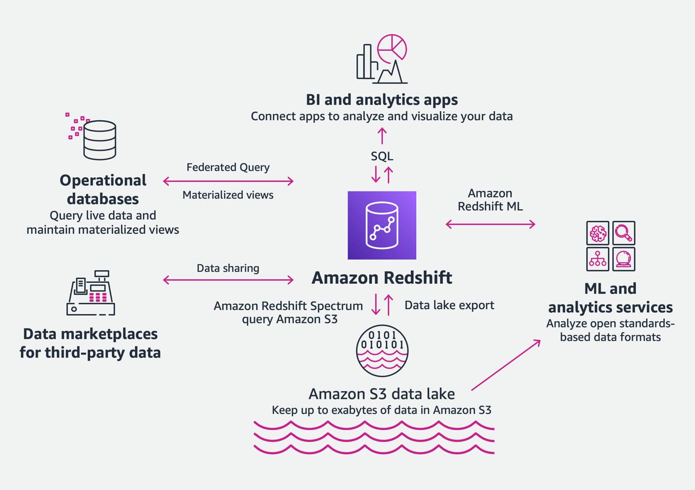
Amazon Redshift allows you to easily analyze all data types across your data warehouse, operational database, and data lake using standard SQL. In this post, we collect, process, and analyze data streams in real time. With data sharing, you can share live data across Amazon Redshift clusters for read purposes with relative security and ease out of the box. In this post, we discuss how we can harness the data sharing ability of Amazon Redshift to set up a big data Lambda architecture to allow both batch and near-real-time analytics.
Solution overview
Example Corp. is a leading electric automotive company that revolutionized the automotive industry. Example Corp. operationalizes the connected vehicle data and improves the effectiveness of various connected vehicle and fleet use cases, including predictive maintenance, in-vehicle service monetization, usage-based insurance. and delivering exceptional driver experiences. In this post, we explore the real-time and trend analytics using the connected vehicle data to illustrate the following use cases:
- Usage-based insurance – Usage-based insurance (UBI) relies on analysis of near-real-time data from the driver’s vehicle to access the risk profile of the driver. In addition, it also relies on the historical analysis (batch) of metrics (such as the number of miles driven in a year). The better the driver, the lower the premium.
- Fleet performance trends – The performance of a fleet (such as a taxi fleet) relies on the analysis of historical trends of data across the fleet (batch) as well as the ability to drill down to a single vehicle within the fleet for near-real-time analysis of metrics like fuel consumption or driver distraction.
Architecture overview
In this section, we discuss the overall architectural setup for the Lambda architecture solution.
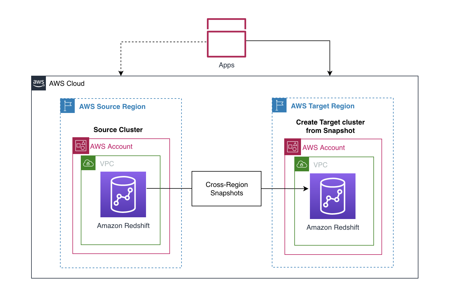
The following diagram shows the implementation architecture and the different computational layers:
- Data ingestion from AWS IoT Core
- Batch layer
- Speed layer
- Serving layer

Data ingestion
Vehicle telemetry data is ingested into the cloud through AWS IoT Core and routed to Amazon Kinesis Data Streams. The Kinesis Data Streams layer acts as a separation layer for the speed layer and batch layer, where the incoming telemetry is consumed by the speed layer’s Amazon Redshift cluster and Amazon Kinesis Data Firehose, respectively.
Batch layer
Amazon Kinesis Data Firehose is a fully managed service that can batch, compress, transform, and encrypt your data streams before loading them into your Amazon Simple Storage Service (Amazon S3) data lake. Kinesis Data Firehose also allows you to specify a custom expression for the Amazon S3 prefix where data records are delivered. This provides the ability to filter the partitioned data and control the amount of data scanned by each query, thereby improving performance and reducing cost.
The batch layer persists data in Amazon S3 and is accessed directly by an Amazon Redshift Serverless endpoint (serving layer). With Amazon Redshift Serverless, you can efficiently query and retrieve structured and semistructured data from files in Amazon S3 without having to load the data into Amazon Redshift tables.
The batch layer can also optionally precompute results as batch views from the immutable Amazon S3 data lake and persist them as either native tables or materialized views for very high-performant use cases. You can create these precomputed batch views using AWS Glue, Amazon Redshift stored procedures, Amazon Redshift materialized views, or other options.
The batch views can be calculated as:
In this solution, we build a batch layer for Example Corp. for two types of queries:
- rapid_acceleration_by_year – The number of rapid accelerations by each driver aggregated per year
- total_miles_driven_by_year – The total number of miles driven by the fleet aggregated per year
For demonstration purposes, we use Amazon Redshift stored procedures to create the batch views as Amazon Redshift native tables from external tables using Amazon Redshift Spectrum.
Speed layer
The speed layer processes data streams in real time and aims to minimize latency by providing real-time views into the most recent data.
Amazon Redshift Streaming Ingestion uses SQL to connect with one or more Kinesis data streams simultaneously. The native streaming ingestion feature in Amazon Redshift lets you ingest data directly from Kinesis Data Streams and enables you to ingest hundreds of megabytes of data per second and query it at exceptionally low latency—in many cases only 10 seconds after entering the data stream.
The speed cluster uses materialized views to materialize a point-in-time view of a Kinesis data stream, as accumulated up to the time it is queried. The real-time views are computed using this layer, which provide a near-real-time view of the incoming telemetry stream.
The speed views can be calculated as a function of recent data unaccounted for in the batch views:
We calculate the speed views for these batch views as follows:
- rapid_acceleration_realtime – The number of rapid accelerations by each driver for recent data not accounted for in the batch view
rapid_acceleration_by_month - miles_driven_realtime – The number of miles driven by each driver for recent data not in
miles_driven_by_month
Serving layer
The serving layer comprises an Amazon Redshift Serverless endpoint and any consumption services such as Amazon QuickSight or Amazon SageMaker.
Amazon Redshift Serverless (preview) is a serverless option of Amazon Redshift that makes it easy to run and scale analytics in seconds without the need to set up and manage data warehouse infrastructure. With Amazon Redshift Serverless, any user—including data analysts, developers, business professionals, and data scientists—can get insights from data by simply loading and querying data in the data warehouse.
Amazon Redshift data sharing enables instant, granular, and fast data access across Amazon Redshift clusters without the need to maintain redundant copies of data.
The speed cluster provides outbound data shares of the real-time materialized views to the Amazon Redshift Serverless endpoint (serving cluster).
The serving cluster joins data from the batch layer and speed layer to get near-real-time and historical data for a particular function with minimal latency. The consumption layer (such as Amazon API Gateway or QuickSight) is only aware of the serving cluster, and all the batch and stream processing is abstracted from the consumption layer.
We can view the queries to the speed layer from data consumption layer as follows:
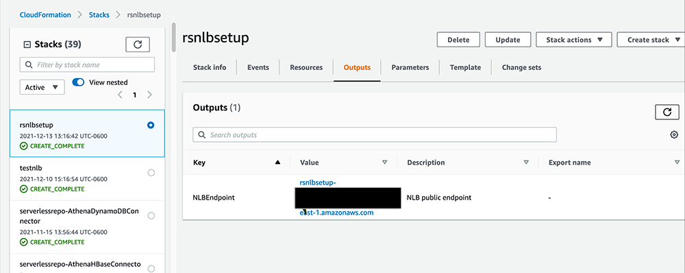
Deploy the CloudFormation template
We have provided an AWS CloudFormation template to demonstrate the solution. You can download and use this template to easily deploy the required AWS resources. This template has been tested in the us-east-1 Region.
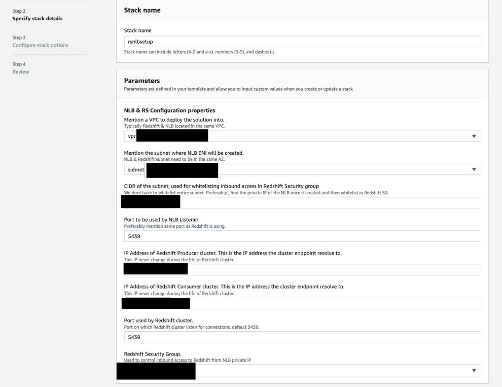
The template requires you to provide the following parameters:
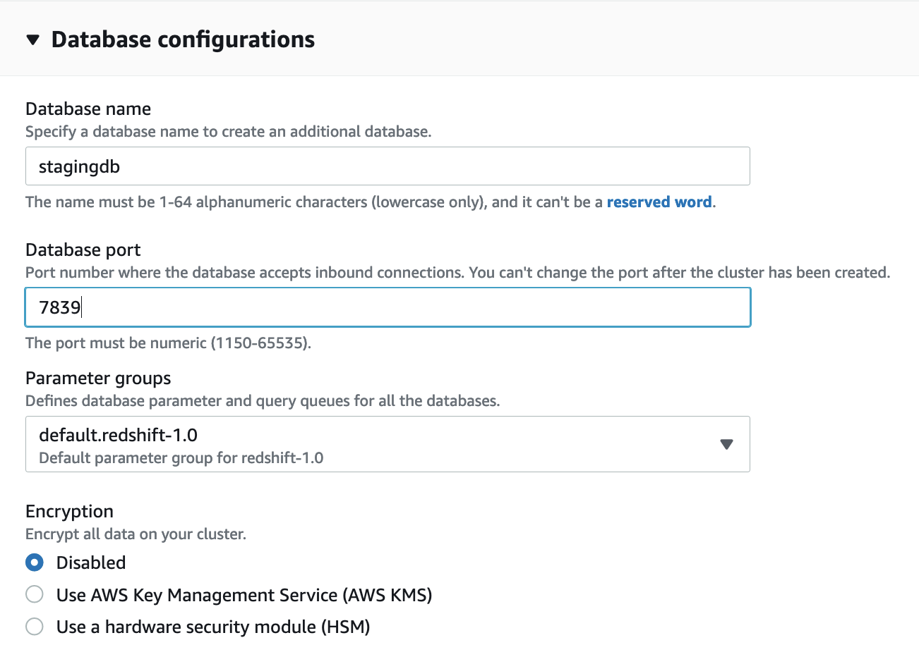
- DatabaseName – The name of the first database to be created for speed cluster
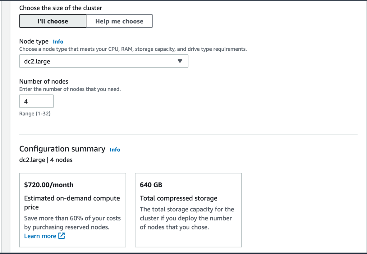
- NumberOfNodes – The number of compute nodes in the cluster.
- NodeType – The type of node to be provisioned
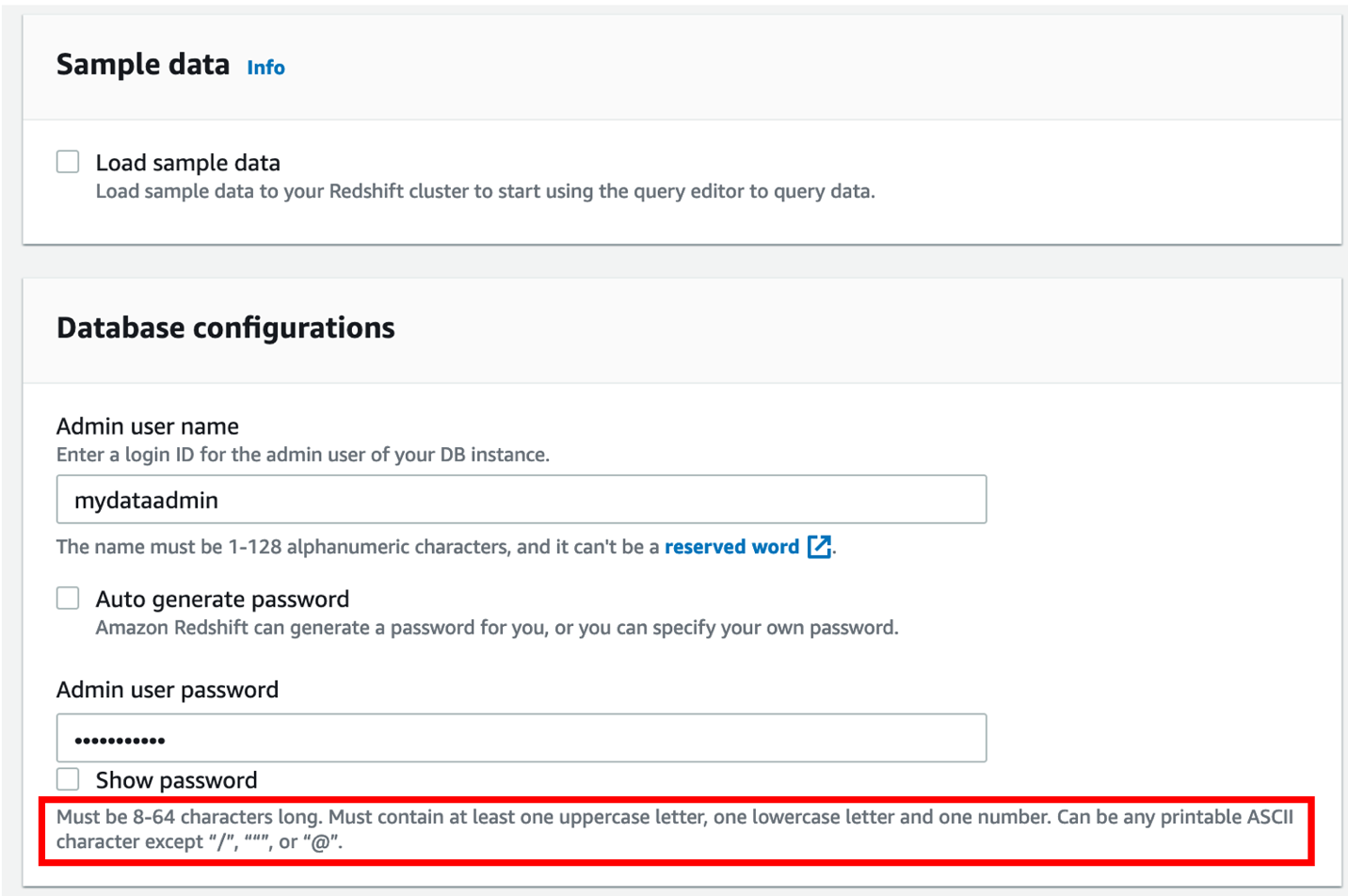
- MasterUserName – The user name that is associated with the master user account for the cluster that is being created
- MasterUserPassword – The password that is associated with the master user account
- InboundTraffic – The CIDR range to allow inbound traffic to the cluster
- PortNumber – The port number on which the cluster accepts incoming connections
- SQLForData – The source query to extract from AWS IOT Core topic
Prerequisites
When setting up this solution and using your own application data to push to Kinesis Data Streams, you can skip setting up the IoT Device Simulator and start creating your Amazon Redshift Serverless endpoint. This post uses the simulator to create related database objects and assumes use of the simulator in the solution walkthrough.
Set up the IoT Device Simulator
We use the IoT Device simulator to generate and simulate vehicle IoT data. The solution allows you to create and simulate hundreds of connected devices, without having to configure and manage physical devices or develop time-consuming scripts.
Use the following CloudFormation template to create the IoT Device Simulator in your account for trying out this solution.
Configure devices and simulations
To configure your devices and simulations, complete the following steps:
- Use the login information you received in the email you provided to log in to the IoT Device Simulator.
- Choose Device Types and Add Device Type.
- Choose Automotive Demo.
- For Device type name, enter
testVehicles. - For Topic, enter the topic where the sensor data is sent to AWS IoT Core.

- Save your settings.
- Choose Simulations and Add simulation.
- For Simulation name, enter
testSimulation. - For Simulation type¸ choose Automotive Demo.
- For Select a device type¸ choose the device type you created (
testVehicles). - For Number of devices, enter
15.

You can choose up to 100 devices per simulation. You can configure a higher number of devices to simulate large data.
- For Data transmission interval, enter
1. - For Data transmission duration, enter
300.
This configuration runs the simulation for 5 minutes.
- Choose Save.


Now you’re ready to simulate vehicle telemetry data to AWS IoT Core.
Create an Amazon Redshift Serverless endpoint
The solution uses an Amazon Redshift Serverless endpoint as the serving layer cluster. You can set up Amazon Redshift Serverless in your account.
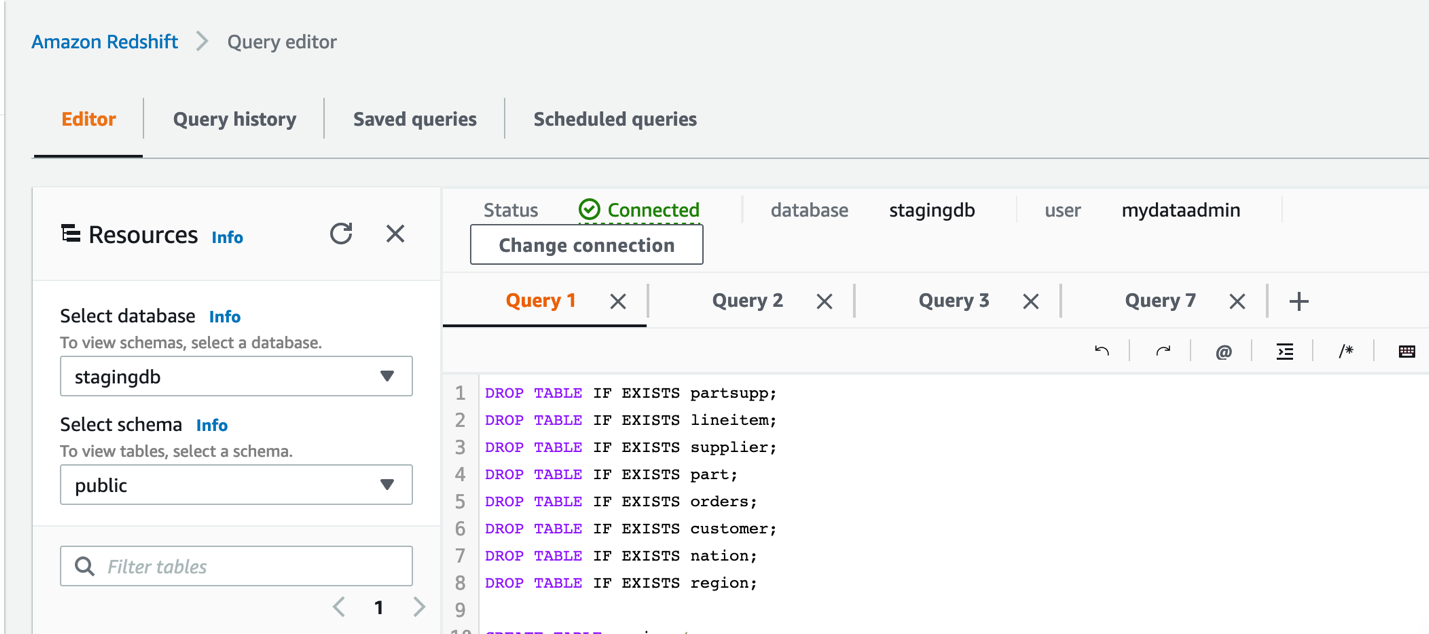
Set up Amazon Redshift Query Editor V2
To query data, you can use Amazon Redshift Query Editor V2. For more information, refer to Introducing Amazon Redshift Query Editor V2, a Free Web-based Query Authoring Tool for Data Analysts.
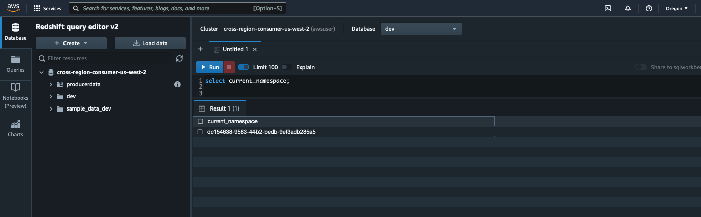
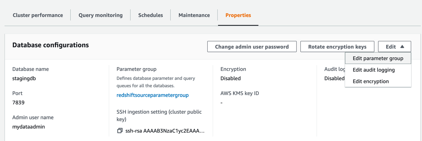
Get namespaces for the provisioned speed layer cluster and Amazon Redshift Serverless
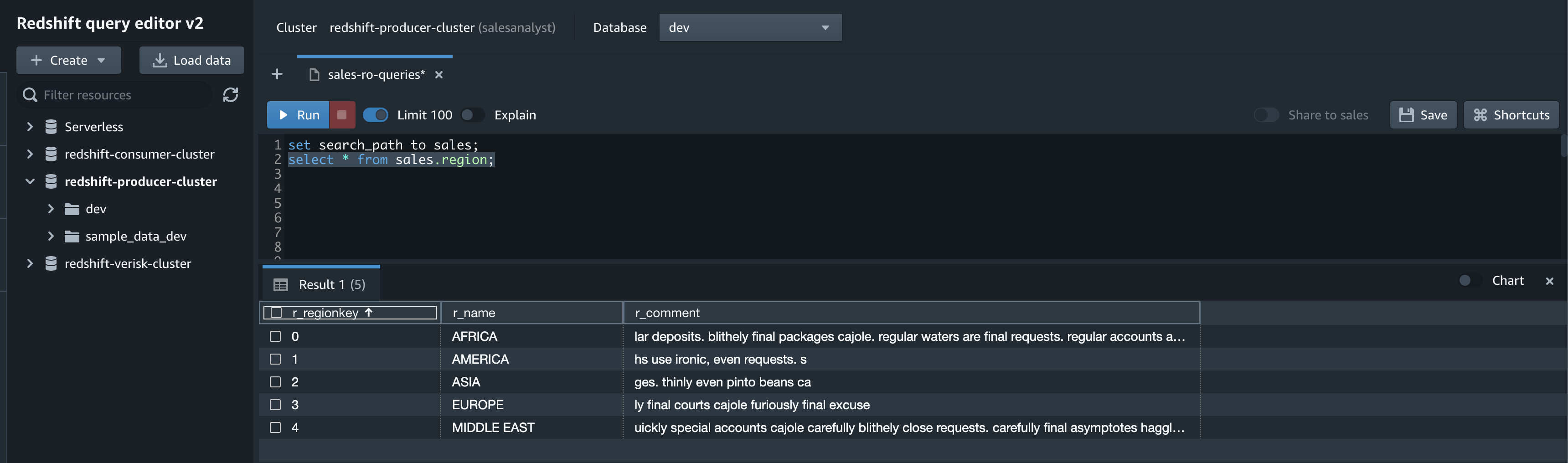
Connect to speed-cluster-iot (the speed layer cluster) through Query Editor V2 and run the following SQL:
Similarly, connect to the Amazon Redshift Serverless endpoint and get the namespace:
You can also get this information via the Amazon Redshift console.
Now that we have all the prerequisites set up, let’s go through the solution walkthrough.
Implement the solution
The workflow includes the following steps:
- Start the IoT simulation created in the previous section.
The vehicle IoT is simulated and ingested through IoT Device Simulator for the configured number of vehicles. The raw telemetry payload is sent to AWS IoT Core, which routes the data to Kinesis Data Streams.
At the batch layer, data is directly put from Kinesis Data Streams to Kinesis Data Firehose, which converts the data to parquet and delivers to Amazon with the prefix s3://<Bucketname>/vehicle_telematics_raw/year=<>/month=<>/day=<>/.
- When the simulation is complete, run the pre-created AWS Glue crawler
vehicle_iot_crawleron the AWS Glue console.
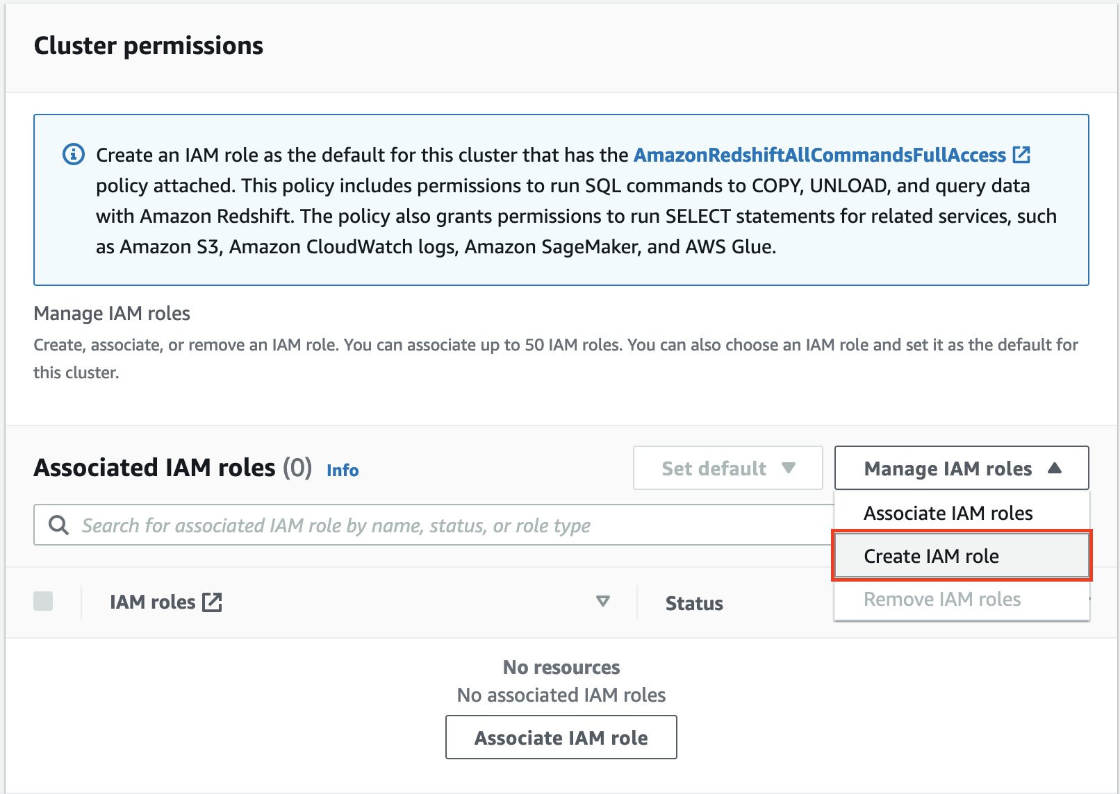
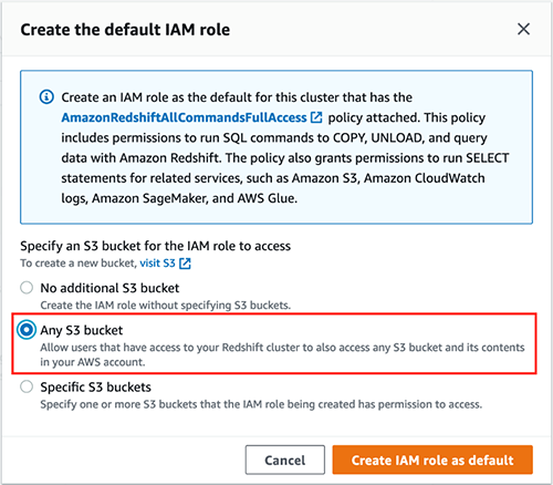
The serving layer Amazon Redshift Serverless endpoint can directly access data from the Amazon S3 data lake through Redshift Spectrum external tables. In this demo, we compute batch views through Redshift Spectrum and store them as Amazon Redshift tables using Amazon Redshift stored procedures.
- Connect to the Amazon Redshift Serverless endpoint through Query Editor V2 and create the stored procedures using the following SQL script.
- Run the two stored procedures to create the batch views:
The two stored procedures create batch views as Amazon Redshift native tables:
-
batchlayer_rapid_acceleration_by_yearbatchlayer_total_miles_by_year
You can also schedule these stored procedures as batch jobs. For more information, refer to Scheduling SQL queries on your Amazon Redshift data warehouse.
At the speed layer, the incoming data stream is read and materialized by the speed layer Amazon Redshift cluster in the materialized view vehicleiotstream_mv.
- Connect to the provisioned
speed-cluster-iotand run the following SQL script to create the required objects.
Two real-time views are created from this materialized view:
-
batchlayer_rapid_acceleration_by_yearbatchlayer_total_miles_by_year
- Refresh the materialized view
vehicleiotstream_mvat the required interval, which triggers Amazon Redshift to read from the stream and load data into the materialized view.
Refreshes are currently manual, but can be automated using the query scheduler.
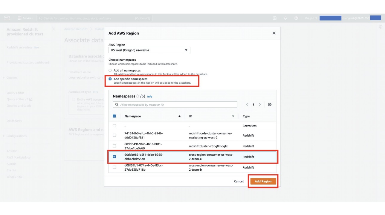
The real-time views are shared as an outbound data share by the speed cluster to the serving cluster.
- Connect to
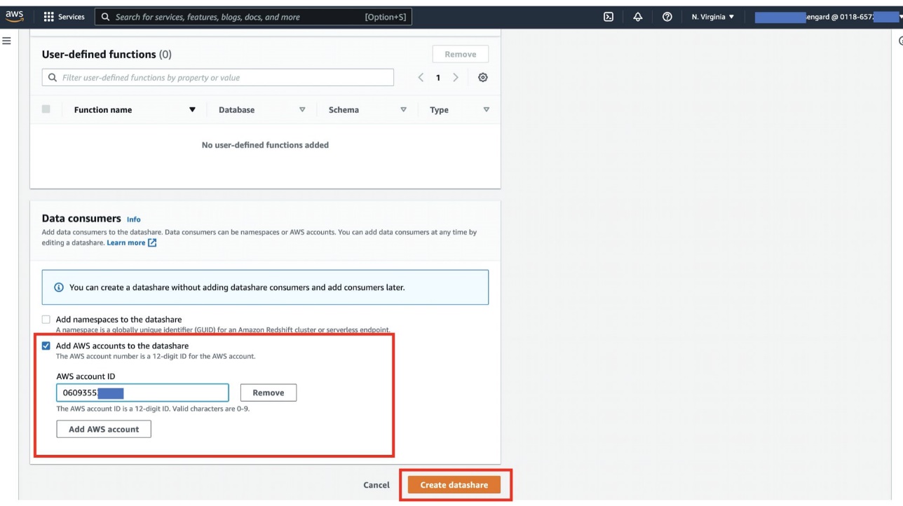
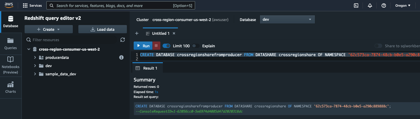
speed-cluster-iotand create an outbound data share (producer) with the following SQL: - Connect to
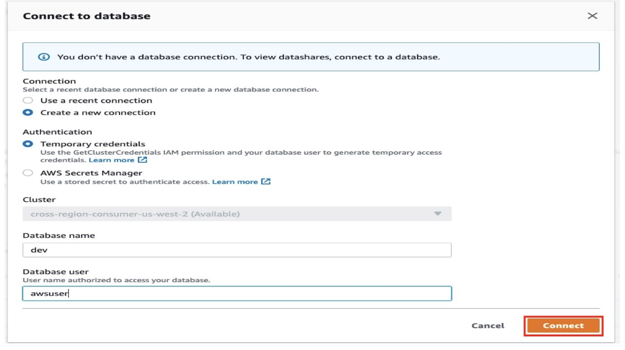
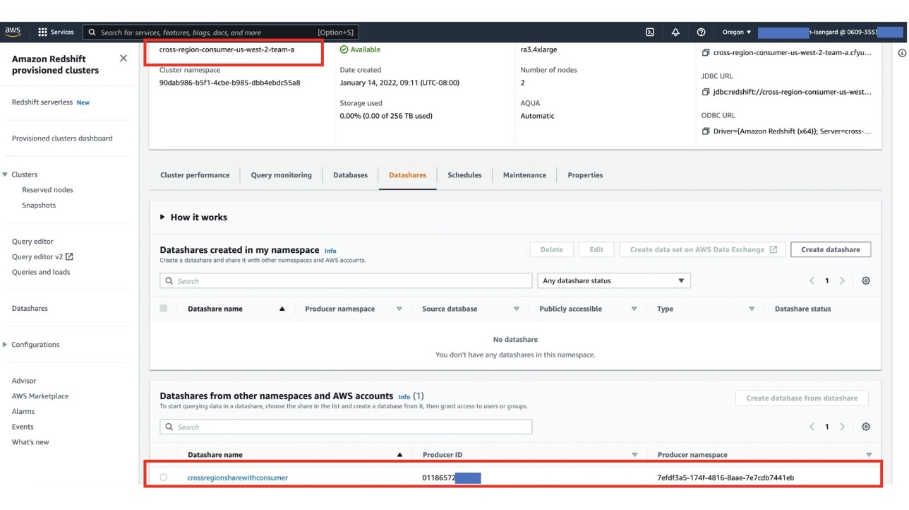
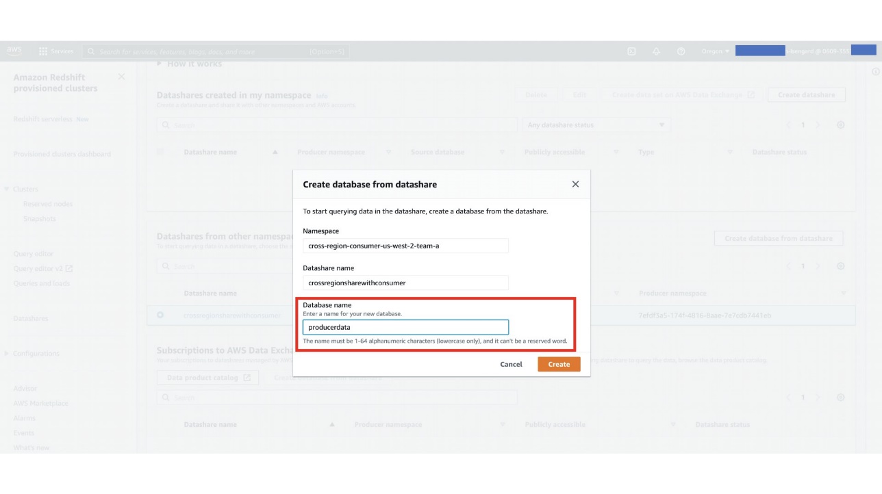
speed-cluster-iotand create an inbound data share (consumer) with the following SQL:
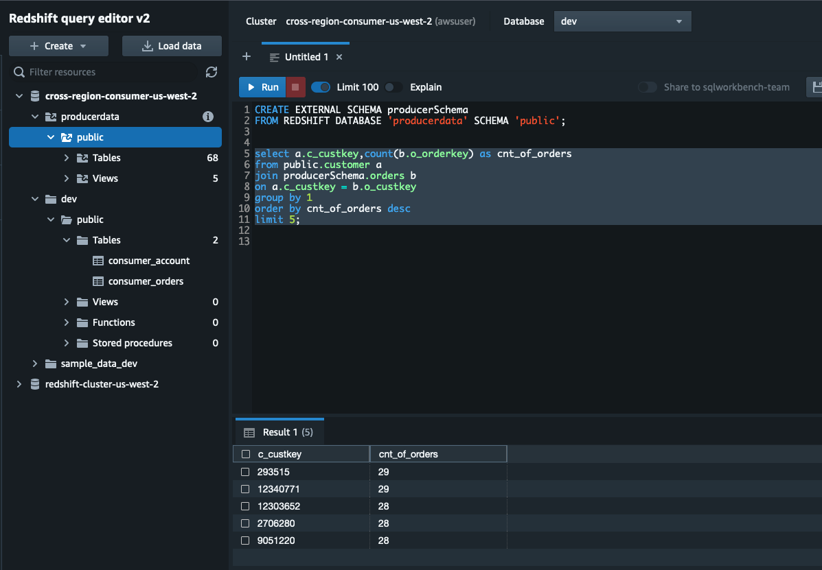
Now that the real-time views are available for the Amazon Redshift Serverless endpoint, we can run queries to get real-time metrics or historical trends with up-to-date data by accessing the batch and speed layers and joining them using the following queries.
For example, to calculate total rapid acceleration by year with up-to-the-minute data, you can run the following query:
Similarly, to calculate total miles driven by year with up-to-the-minute data, run the following query:
For only access to real-time data to power daily dashboards, you can run queries against real-time views shared to your Amazon Redshift Serverless cluster.
For example, to calculate the average speed per trip of your fleet, you can run the following SQL:
Because this demo uses the same data as a quick start, there are duplicates in this demonstration. In actual implementations, the serving cluster manages the data redundancy and duplication by creating views with date predicates that consume non-overlapping data from batch and real-time views and provide overall metrics to the consumption layer.
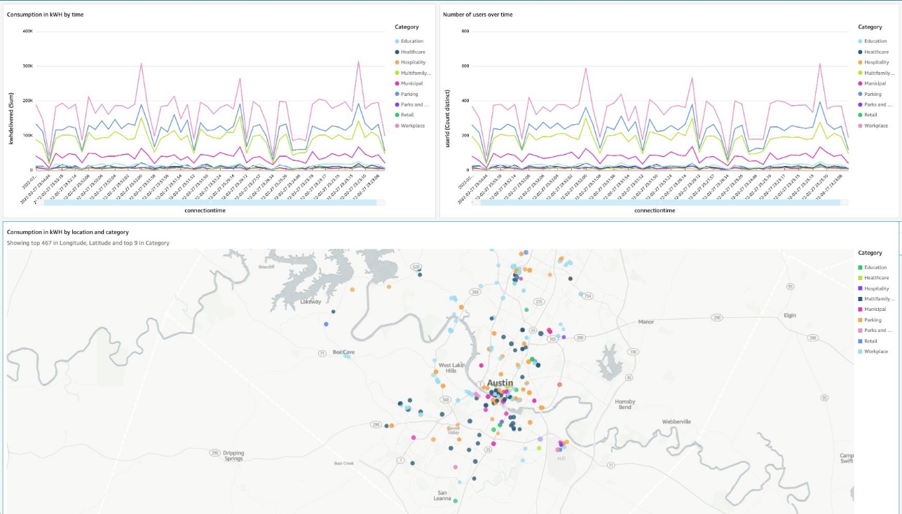
You can consume the data with QuickSight for dashboards, with API Gateway for API-based access, or via the Amazon Redshift Data API or SageMaker for AI and machine learning (ML) workloads. This is not included as part of the provided CloudFormation template.
Best practices
In this section, we discuss some best practices and lessons learned when using this solution.
Provisioned vs. serverless
The speed layer is a continuous ingestion layer reading data from the IoT streams often running 24/7 workloads. There is less idle time and variability in the workloads and it is advantageous to have a provisioned cluster supporting persistent workloads that can scale elastically.
The serving layer can be provisioned (in case of 24/7 workloads) or Amazon Redshift Serverless in case of sporadic or ad hoc workloads. In this post, we assumed sporadic workloads, so serverless is the best fit. In addition, the serving layer can house multiple Amazon Redshift clusters, each consuming their data share and serving downstream applications.
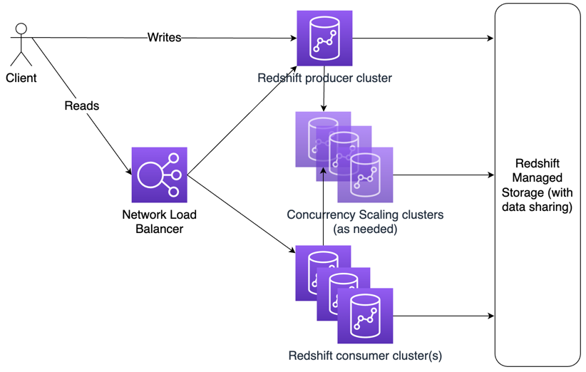
RA3 instances for data sharing
Amazon Redshift RA3 instances enable data sharing to allow you to securely and easily share live data across Amazon Redshift clusters for reads. You can combine the data that is ingested in near-real time with the historical data using the data share to provide personalized driving characteristics to determine the insurance recommendation.
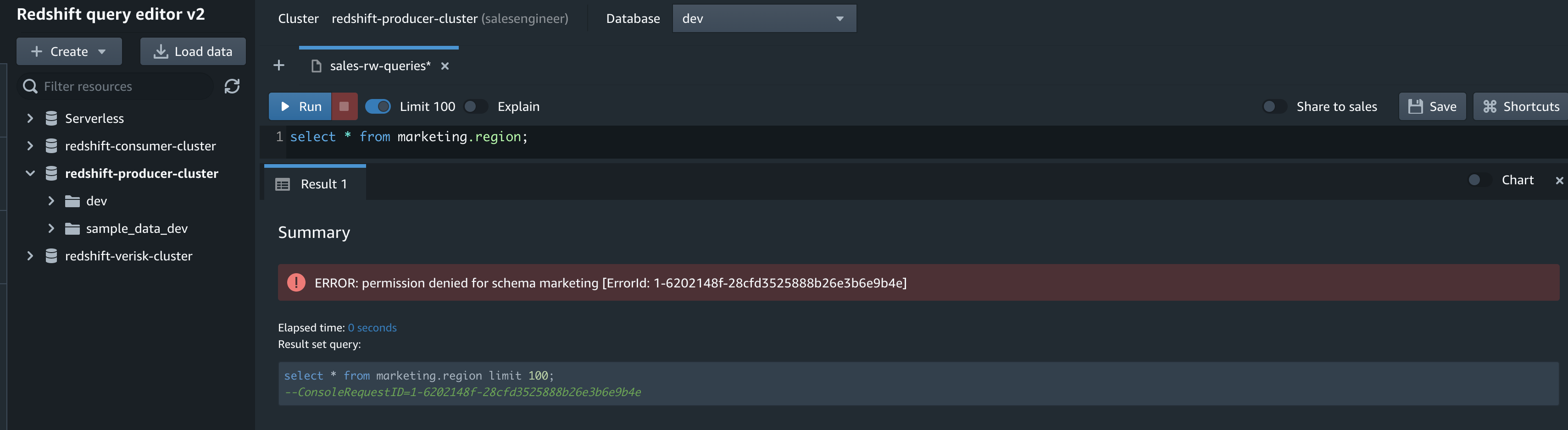
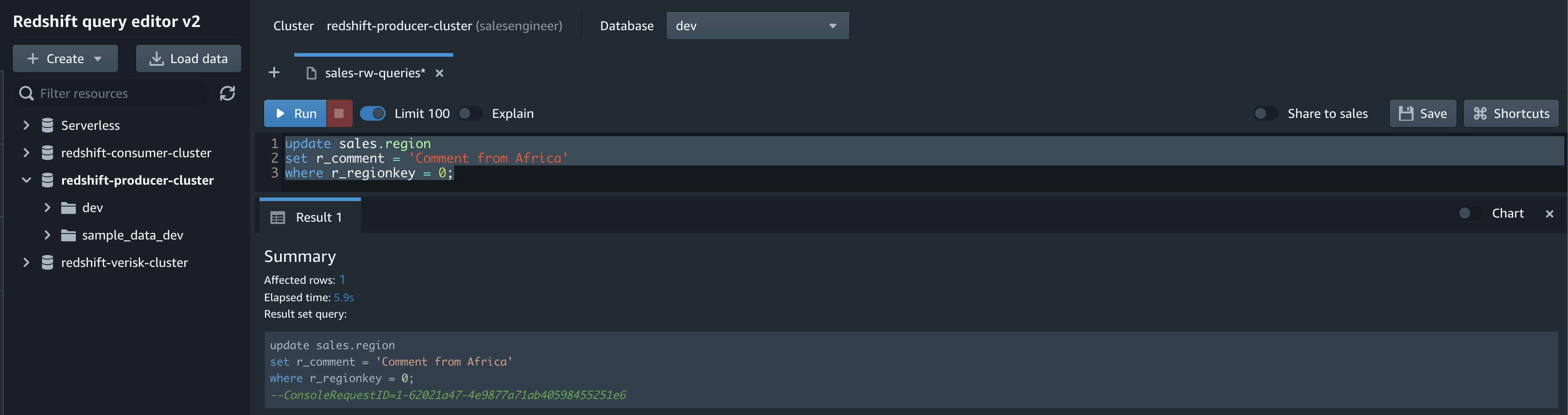
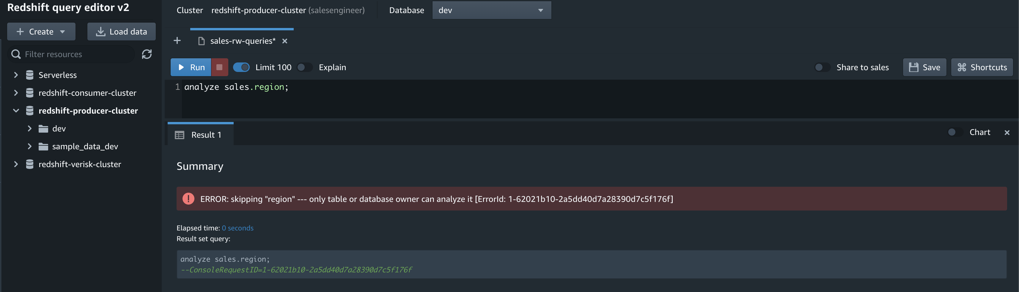
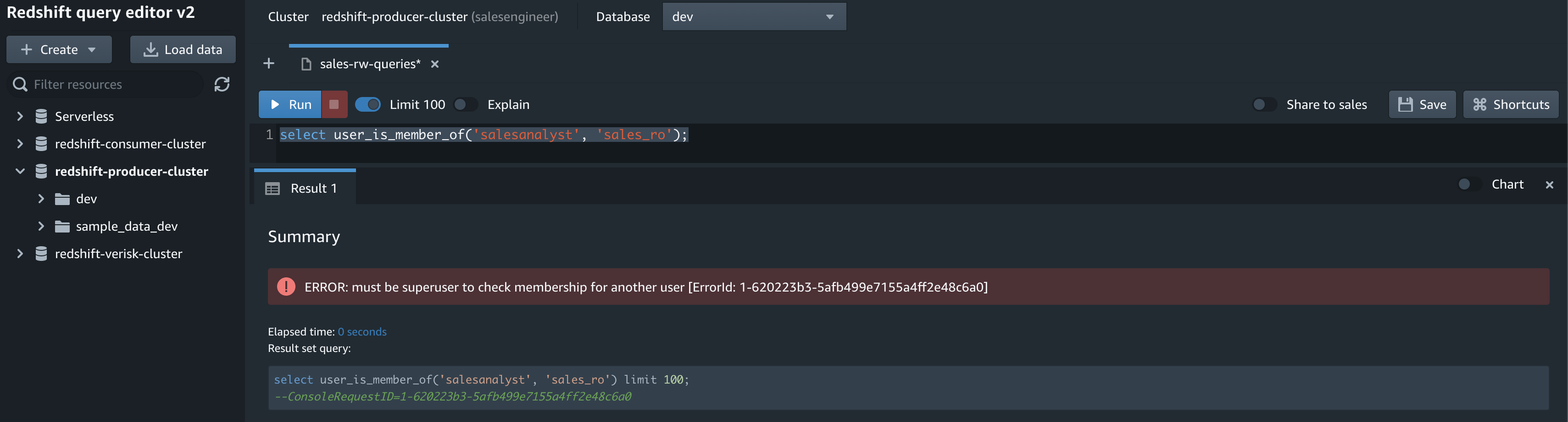
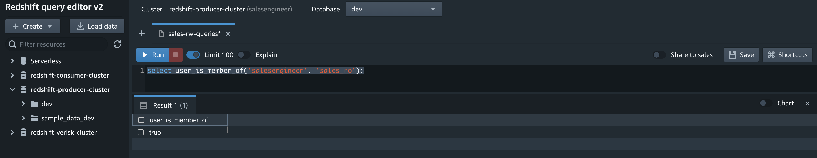
You can also grant fine-grained access control to the underlying data in the producer to the consumer cluster as needed. Amazon Redshift offers comprehensive auditing capabilities using system tables and AWS CloudTrail to allow you to monitor the data sharing permissions and usage across all the consumers and revoke access instantly when necessary. The permissions are granted by the superusers from both the producer and the consumer clusters to define who gets access to what objects, similar to the grant commands used in the earlier section. You can use the following commands to audit the usage and activities for the data share.
Track all changes to the data share and the shared database imported from the data share with the following code:
Track data share access activity (usage), which is relevant only on the producer, with the following code:
Pause and Resume
You can pause the producer cluster when batch processing is complete to save costs. The pause and resume actions on Amazon Redshift allow you to easily pause and resume clusters that may not be in operation at all times. It allows you to create a regularly-scheduled time to initiate the pause and resume actions at specific times or you can manually initiate a pause and later a resume. Flexible on-demand pricing and per-second billing gives you greater control of costs of your Redshift compute clusters while maintaining your data in a way that is simple to manage.
Materialized views for fast access to data
Materialized views allow pre-composed results from complex queries on large tables for faster access. The producer cluster exposes data as materialized views to simplify access for the consumer cluster. This also allows flexibility at the producer cluster to update the underlying table structure to address new business use cases, without affecting consumer-dependent queries and enabling a loose coupling.
Conclusion
In this post, we demonstrated how to process and analyze large-scale data from streaming and batch sources using Amazon Redshift as the core of the platform guided by the Lambda architecture principles.
You started by collecting real-time data from connected vehicles, and storing the streaming data in an Amazon S3 data lake through Kinesis Data Firehose. The solution simultaneously processes the data for near-real-time analysis through Amazon Redshift streaming ingestion.
Through the data sharing feature, you were able to share live, up-to-date data to an Amazon Redshift Serverless endpoint (serving cluster), which merges the data from the speed layer (near-real time) and batch layer (batch analysis) to provide low-latency access to data from near-real-time analysis to historical trends.
Click here to get started with this solution today and let us know how you implemented this solution in your organization through the comments section.
About the Authors
 Jagadish Kumar is a Sr Analytics Specialist Solutions Architect at AWS. He is deeply passionate about Data Architecture and helps customers build analytics solutions at scale on AWS. He is an avid college football fan and enjoys reading, watching sports and riding motorcycle.
 Thiyagarajan Arumugam is a Big Data Solutions Architect at Amazon Web Services and designs customer architectures to process data at scale. Prior to AWS, he built data warehouse solutions at Amazon.com. In his free time, he enjoys all outdoor sports and practices the Indian classical drum mridangam.
 Eesha Kumar is an Analytics Solutions Architect with AWS. He works with customers to realize business value of data by helping them building solutions leveraging AWS platform and tools.


 Stefan Gromoll is a Senior Performance Engineer with Amazon Redshift where he is responsible for measuring and improving Redshift performance. In his spare time, he enjoys cooking, playing with his three boys, and chopping firewood.


 Roy Hasson is the Head of Product at Upsolver. He works with customers globally to simplify how they build, manage and deploy data pipelines to deliver high quality data as a product. Previously, Roy was a Product Manager for AWS Glue and AWS Lake Formation.
 Mei Long is a Product Manager at Upsolver. She is on a mission to make data accessible, usable and manageable in the cloud. Previously, Mei played an instrumental role working with the teams that contributed to the Apache Hadoop, Spark, Zeppelin, Kafka, and Kubernetes projects.


 Chris King is a Principal Solutions Architect in Applied AI with AWS. He has a special interest in launching AI services and helped grow and build Amazon Personalize and Amazon Forecast before focusing on Amazon Lookout for Metrics. In his spare time he enjoys cooking, reading, boxing, and building models to predict the outcome of combat sports.
 Alex Kim is a Sr. Product Manager for Amazon Forecast. His mission is to deliver AI/ML solutions to all customers who can benefit from it. In his free time, he enjoys all types of sports and discovering new places to eat.


