Tag Archives: AWS Database Migration Service

Create a low-latency source-to-data lake pipeline using Amazon MSK Connect, Apache Flink, and Apache Hudi

Post Syndicated from Ali Alemi original https://aws.amazon.com/blogs/big-data/create-a-low-latency-source-to-data-lake-pipeline-using-amazon-msk-connect-apache-flink-and-apache-hudi/

During the recent years, there has been a shift from monolithic to the microservices architecture. The microservices architecture makes applications easier to scale and quicker to develop, enabling innovation and accelerating time to market for new features. However, this approach causes data to live in different silos, which makes it difficult to perform analytics. To gain deeper and richer insights, you should bring all your data from different silos into one place.

AWS offers replication tools such as AWS Database Migration Service (AWS DMS) to replicate data changes from a variety of source databases to various destinations including Amazon Simple Storage Service (Amazon S3). But customers who need to sync the data in a data lake with updates and deletes on the source systems still face a few challenges:

  • It’s difficult to apply record-level updates or deletes when records are stored in open data format files (such as JSON, ORC, or Parquet) on Amazon S3.
  • In streaming use cases, where jobs need to write data with low latency, row-based formats such as JSON and Avro are best suited. However, scanning many small files with these formats degrades the read query performance.
  • In use cases where the schema of the source data changes frequently, maintaining the schema of the target datasets via custom code is difficult and error-prone.

Apache Hudi provides a good way to solve these challenges. Hudi builds indexes when it writes the records for the first time. Hudi uses these indexes to locate the files to which an update (or delete) belongs. This enables Hudi to perform fast upsert (or delete) operations by avoiding the need to scan the whole dataset. Hudi provides two table types, each optimized for certain scenarios:

  • Copy-On-Write (COW) – These tables are common for batch processing. In this type, data is stored in a columnar format (Parquet), and each update (or delete) creates a new version of files during the write.
  • Merge-On-Read (MOR) – Stores Data using a combination of columnar (for example Parquet) and row-based (for example Avro) file formats and is intended to expose near-real time data.

Hudi datasets stored in Amazon S3 provide native integration with other AWS services. For example, you can write Apache Hudi tables using AWS Glue (see Writing to Apache Hudi tables using AWS Glue Custom Connector) or Amazon EMR (see New features from Apache Hudi available in Amazon EMR). Those approaches require having a deep understanding of Hudi’s Spark APIs and programming skills to build and maintain data pipelines.

In this post, I show you a different way of working with streaming data with minimum coding. The steps in this post demonstrate how to build fully scalable pipelines using SQL language without prior knowledge of Flink or Hudi. You can query and explore your data in multiple data streams by writing familiar SELECT queries. You can join the data from multiple streams and materialize the result to a Hudi dataset on Amazon S3.

Solution overview

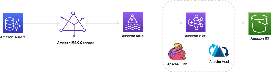
The following diagram provides an overall architecture of the solution described in this post. I describe the components and steps fully in the sections that follow.

You use an Amazon Aurora MySQL database as the source and a Debezium MySQL connector with the setup described in the MSK Connect lab as the change data capture (CDC) replicator. This lab walks you through the steps to set up the stack for replicating an Aurora database salesdb to an Amazon Managed Streaming for Apache Kafka (Amazon MSK) cluster, using Amazon MSK Connect with a MySql Debezium source Kafka connector.

In September 2021, AWS announced MSK Connect for running fully managed Kafka Connect clusters. With a few clicks, MSK Connect allows you to easily deploy, monitor, and scale connectors that move data in and out of Apache Kafka and MSK clusters from external systems such as databases, file systems, and search indexes. You can now use MSK Connect for building a full CDC pipeline from many database sources to your MSK cluster.

Amazon MSK is a fully managed service that makes it easy to build and run applications that use Apache Kafka to process streaming data. When you use Apache Kafka, you capture real-time data from sources such as database change events or website clickstreams. Then you build pipelines (using stream processing frameworks such as Apache Flink) to deliver them to destinations such as a persistent storage or Amazon S3.

Apache Flink is a popular framework for building stateful streaming and batch pipelines. Flink comes with different levels of abstractions to cover a broad range of use cases. See Flink Concepts for more information.

Flink also offers different deployment modes depending on which resource provider you choose (Hadoop YARN, Kubernetes, or standalone). See Deployment for more information.

In this post, you use the SQL Client tool as an interactive way of authoring Flink jobs in SQL syntax. sql-client.sh compiles and submits jobs to a long-running Flink cluster (session mode) on Amazon EMR. Depending on the script, sql-client.sh either shows the tabular formatted output of the job in real time, or returns a job ID for long-running jobs.

You implement the solution with the following high-level steps:

  1. Create an EMR cluster.
  2. Configure Flink with Kafka and Hudi table connectors.
  3. Develop your real-time extract, transform, and load (ETL) job.
  4. Deploy your pipeline to production.

Prerequisites

This post assumes you have a running MSK Connect stack in your environment with the following components:

  • Aurora MySQL hosting a database. In this post, you use the example database salesdb.
  • The Debezium MySQL connector running on MSK Connect, ending in Amazon MSK in your Amazon Virtual Private Cloud (Amazon VPC).
  • An MSK cluster running within in a VPC.

If you don’t have an MSK Connect stack, follow the instructions in the MSK Connect lab setup and verify that your source connector replicates data changes to the MSK topics.

You also need the ability to connect directly to the EMR leader node. Session Manager is a feature of AWS Systems Manager that provides you with an interactive one-click browser-based shell window. Session Manager also allows you to comply with corporate policies that require controlled access to managed nodes. See Setting up Session Manager to learn how to connect to your managed nodes in your account via this method.

If Session Manager is not an option, you can also use Amazon Elastic Compute Cloud (Amazon EC2) private key pairs, but you’ll need to launch the cluster in a public subnet and provide inbound SSH access. See Connect to the master node using SSH for more information.

Create an EMR cluster

The latest released version of Apache Hudi is 0.10.0, at the time of writing. Hudi release version 0.10.0 is compatible with Flink release version 1.13. You need Amazon EMR release version emr-6.4.0 and later, which comes with Flink release version 1.13. To launch a cluster with Flink installed using the AWS Command Line Interface (AWS CLI), complete the following steps:

  1. Create a file, configurations.json, with the following content:
    [
        {
          "Classification": "flink-conf",
          "Properties": {
            "taskmanager.numberOfTaskSlots":"4"
          }
        }
    ]

  2. Create an EMR cluster in a private subnet (recommended) or in a public subnet of the same VPC as where you host your MSK cluster. Enter a name for your cluster with the --name option, and specify the name of your EC2 key pair as well as the subnet ID with the --ec2-attributes option. See the following code:
    aws emr create-cluster --release-label emr-6.4.0 \
    --applications Name=Flink \
    --name FlinkHudiCluster \
    --configurations file://./configurations.json \
    --region us-east-1 \
    --log-uri s3://yourLogUri \
    --instance-type m5.xlarge \
    --instance-count 2 \
    --service-role EMR_DefaultRole \ 
    --ec2-attributes KeyName=YourKeyName,InstanceProfile=EMR_EC2_DefaultRole, SubnetId=A SubnetID of Amazon MSK VPC 

  3. Wait until the cluster state changes to Running.
  4. Retrieve the DNS name of the leader node using either the Amazon EMR console or the AWS CLI.
  5. Connect to the leader node via Session Manager or using SSH and an EC2 private key on Linux, Unix, and Mac OS X.
  6. When connecting using SSH, port 22 must be allowed by the leader node’s security group.
  7. Make sure the MSK cluster’s security group has an inbound rules that accepts traffic from the EMR cluster’s security groups.

Configure Flink with Kafka and Hudi table connectors

Flink table connectors allow you to connect to external systems when programming your stream operations using Table APIs. Source connectors provide access to streaming services including Kinesis or Apache Kafka as a data source. Sink connectors allow Flink to emit stream processing results to external systems or storage services like Amazon S3.

On your Amazon EMR leader node, download the following connectors and save them in the /lib/flink/lib directory:

  • Source connector – Download flink-connector-kafka_2.11-1.13.1.jar from the Apache repository. The Apache Kafka SQL connector allows Flink to read data from Kafka topics.
  • Sink connector – Amazon EMR release version emr-6.4.0 comes with Hudi release version 0.8.0. However, in this post you need Hudi Flink bundle connector release version 0.10.0, which is compatible with Flink release version 1.13. Download hudi-flink-bundle_2.11-0.10.0.jar from the Apache repository. It also contains multiple file system clients, including S3A for integrating with Amazon S3.

Develop your real-time ETL job

In this post, you use the Debezium source Kafka connector to stream data changes of a sample database, salesdb, to your MSK cluster. Your connector produces data changes in JSON. See Debezium Event Deserialization for more details. The Flink Kafka connector can deserialize events in JSON format by setting value.format with debezium-json in the table options. This configuration provides the full support for data updates and deletes, in addition to inserts.

You build a new job using Flink SQL APIs. These APIs allow you to work with the streaming data, similar to tables in relational databases. SQL queries specified in this method run continuously over the data events in the source stream. Because the Flink application consumes unbounded data from a stream, the output constantly changes. To send the output to another system, Flink emits update or delete events to the downstream sink operators. Therefore, when you work with CDC data or write SQL queries where the output rows need to update or delete, you must provide a sink connector that supports these actions. Otherwise, the Flink job ends with an error with the following message:

Target Table doesn't support consuming update or delete changes which is produced by {your query statement} …

Launch the Flink SQL client

Start a Flink YARN application on your EMR cluster with the configurations you previously specified in the configurations.json file:

cd /lib/flink && ./bin/yarn-session.sh --detached

After the command runs successfully, you’re ready to write your first job. Run the following command to launch sql-client:

./bin/sql-client.sh

Your terminal window looks like the following screenshot.

Set the job parameters

Run the following command to set the checkpointing interval for this session:

SET execution.checkpointing.interval = 1min;

Define your source tables

Conceptually, processing streams using SQL queries requires interpreting the events as logical records in a table. Therefore, the first step before reading or writing the data with SQL APIs is to create source and target tables. The table definition includes the connection settings and configuration along with a schema that defines the structure and the serialization format of the objects in the stream.

In this post, you create three source tables. Each corresponds to a topic in Amazon MSK. You also create a single target table that writes the output data records to a Hudi dataset stored on Amazon S3.

Replace BOOTSTRAP SERVERS ADDRESSES with your own Amazon MSK cluster information in the 'properties.bootstrap.servers' option and run the following commands in your sql-client terminal:

CREATE TABLE CustomerKafka (
      `event_time` TIMESTAMP(3) METADATA FROM 'value.source.timestamp' VIRTUAL,  -- from Debezium format
      `origin_table` STRING METADATA FROM 'value.source.table' VIRTUAL, -- from Debezium format
      `record_time` TIMESTAMP(3) METADATA FROM 'value.ingestion-timestamp' VIRTUAL,
      `CUST_ID` BIGINT,
      `NAME` STRING,
      `MKTSEGMENT` STRING,
       WATERMARK FOR event_time AS event_time
    ) WITH (
      'connector' = 'kafka',
      'topic' = 'salesdb.salesdb.CUSTOMER', -- created by debezium connector, corresponds to CUSTOMER table in Amazon Aurora database. 
      'properties.bootstrap.servers' = '<PLAINTEXT BOOTSTRAP SERVERS ADDRESSES>',
      'properties.group.id' = 'ConsumerGroup1',
      'scan.startup.mode' = 'earliest-offset',
      'value.format' = 'debezium-json'
    );

CREATE TABLE CustomerSiteKafka (
      `event_time` TIMESTAMP(3) METADATA FROM 'value.source.timestamp' VIRTUAL,  -- from Debezium format
      `origin_table` STRING METADATA FROM 'value.source.table' VIRTUAL, -- from Debezium format
      `record_time` TIMESTAMP(3) METADATA FROM 'value.ingestion-timestamp' VIRTUAL,
      `CUST_ID` BIGINT,
      `SITE_ID` BIGINT,
      `STATE` STRING,
      `CITY` STRING,
       WATERMARK FOR event_time AS event_time
    ) WITH (
      'connector' = 'kafka',
      'topic' = 'salesdb.salesdb.CUSTOMER_SITE',
      'properties.bootstrap.servers' = '< PLAINTEXT BOOTSTRAP SERVERS ADDRESSES>',
      'properties.group.id' = 'ConsumerGroup2',
      'scan.startup.mode' = 'earliest-offset',
      'value.format' = 'debezium-json'
    );

CREATE TABLE SalesOrderAllKafka (
      `event_time` TIMESTAMP(3) METADATA FROM 'value.source.timestamp' VIRTUAL,  -- from Debezium format
      `origin_table` STRING METADATA FROM 'value.source.table' VIRTUAL, -- from Debezium format
      `record_time` TIMESTAMP(3) METADATA FROM 'value.ingestion-timestamp' VIRTUAL,
      `ORDER_ID` BIGINT,
      `SITE_ID` BIGINT,
      `ORDER_DATE` BIGINT,
      `SHIP_MODE` STRING,
       WATERMARK FOR event_time AS event_time
    ) WITH (
      'connector' = 'kafka',
      'topic' = 'salesdb.salesdb.SALES_ORDER_ALL',
      'properties.bootstrap.servers' = '< PLAINTEXT BOOTSTRAP SERVERS ADDRESSES>',
      'properties.group.id' = 'ConsumerGroup3',
      'scan.startup.mode' = 'earliest-offset',
      'value.format' = 'debezium-json'
    );

By default, sql-client stores these tables in memory. They only live for the duration of the active session. Anytime your sql-client session expires, or you exit, you need to recreate your tables.

Define the sink table

The following command creates the target table. You specify 'hudi' as the connector in this table. The rest of the Hudi configurations are set in the with(…) section of the CREATE TABLE statement. See the full list of Flink SQL configs to learn more. Replace S3URI OF HUDI DATASET LOCATION with your Hudi dataset location in Amazon S3 and run the following code:

CREATE TABLE CustomerHudi (
      `order_count` BIGINT,
      `customer_id` BIGINT,
      `name` STRING,
      `mktsegment` STRING,
      `ts` TIMESTAMP(3),
      PRIMARY KEY (`customer_id`) NOT Enforced
    )
    PARTITIONED BY (`mktsegment`)
    WITH (
      'connector' = 'hudi',
      'write.tasks' = '4',
      'path' = '<S3URI OF HUDI DATASET LOCATION>',
      'table.type' = 'MERGE_ON_READ' --  MERGE_ON_READ table or, by default is COPY_ON_WRITE
    );

Verify the Flink job’s results from multiple topics

For select queries, sql-client submits the job to a Flink cluster, then displays the results on the screen in real time. Run the following select query to view your Amazon MSK data:

SELECT Count(O.order_id) AS order_count,
       C.cust_id,
       C.NAME,
       C.mktsegment
FROM   customerkafka C
       JOIN customersitekafka CS
         ON C.cust_id = CS.cust_id
       JOIN salesorderallkafka O
         ON O.site_id = CS.site_id
GROUP  BY C.cust_id,
          C.NAME,
          C.mktsegment; 

This query joins three streams and aggregates the count of customer orders, grouped by each customer record. After a few seconds, you should see the result in your terminal. Note how the terminal output changes as the Flink job consumes more events from the source streams.

Sink the result to a Hudi dataset

To have a complete pipeline, you need to send the result to a Hudi dataset on Amazon S3. To do that, add an insert into CustomerHudi statement in front of the select query:

INSERT INTO customerhudi
SELECT Count(O.order_id),
       C.cust_id,
       C.NAME,
       C.mktsegment,
       Proctime()
FROM   customerkafka C
       JOIN customersitekafka CS
         ON C.cust_id = CS.cust_id
       JOIN salesorderallkafka O
         ON O.site_id = CS.site_id
GROUP  BY C.cust_id,
          C.NAME,
          C.mktsegment;

This time, the sql-client disconnects from the cluster after submitting the job. The client terminal doesn’t have to wait for the results of the job as it sinks its results to a Hudi dataset. The job continues to run on your Flink cluster even after you stop the sql-client session.

Wait a few minutes until the job generates Hudi commit log files to Amazon S3. Then navigate to the location in Amazon S3 you specified for your CustomerHudi table, which contains a Hudi dataset partitioned by MKTSEGMENT column. Within each partition you also find Hudi commit log files. This is because you defined the table type as MERGE_ON_READ. In this mode with the default configurations, Hudi merges commit logs to larger Parquet files after five delta commit logs occur. Refer to Table & Query Types for more information. You can change this setup by changing the table type to COPY_ON_WRITE or specifying your custom compaction configurations.

Query the Hudi dataset

You may also use a Hudi Flink connector as a source connector to read from a Hudi dataset stored on Amazon S3. You do that by running a select statement against the CustomerHudi table, or create a new table with hudi specified for connector. The path must point to an existing Hudi dataset’s location on Amazon S3. Replace S3URI OF HUDI DATASET LOCATION with your location and run the following command to create a new table:

CREATE TABLE `CustomerHudiReadonly` (
      `_hoodie_commit_time` string,
      `_hoodie_commit_seqno` string,
      `_hoodie_record_key` string,
      `order_count` BIGINT,
      `customer_id` BIGINT,
      `name` STRING,
      `mktsegment` STRING,
      `ts` TIMESTAMP(3),
      PRIMARY KEY (`customer_id`) NOT Enforced
    )
    PARTITIONED BY (`mktsegment`)
    WITH (
      'connector' = 'hudi',
      'hoodie.datasource.query.type' = 'snapshot',
      'path' = '<S3URI OF HUDI DATASET LOCATION>',
     'table.type' = 'MERGE_ON_READ' --  MERGE_ON_READ table or, by default is COPY_ON_WRITE
    );

Note the additional column names prefixed with _hoodie_. These columns are added by Hudi during the write to maintain the metadata of each record. Also note the extra 'hoodie.datasource.query.type'  read configuration passed in the WITH portion of the table definition. This makes sure you read from the real-time view of your Hudi dataset. Run the following command:

Select * from CustomerHudiReadonly where customer_id <= 5;

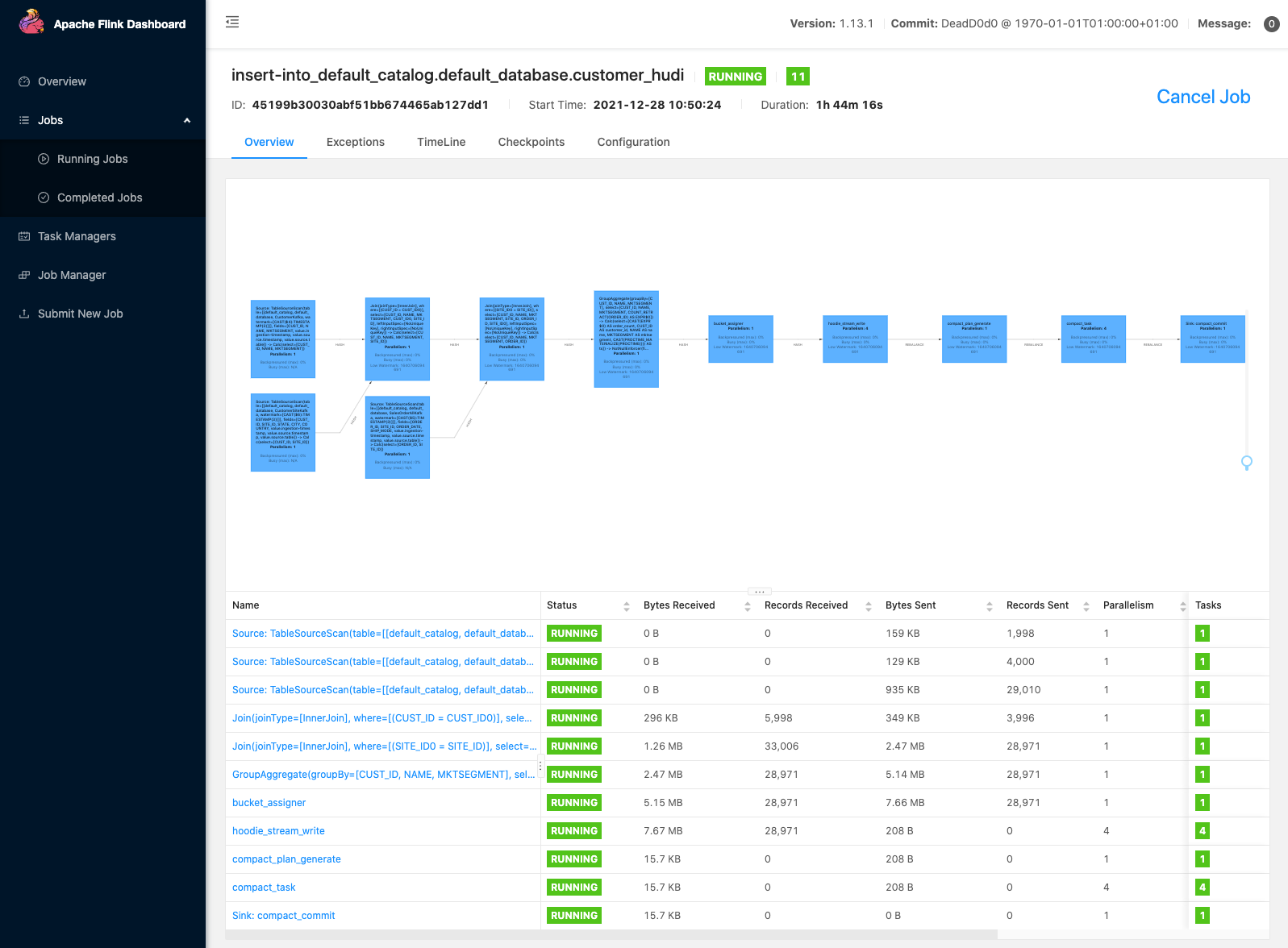
The terminal displays the result within 30 seconds. Navigate to the Flink web interface, where you can observe a new Flink job started by the select query (See below for how to find the Flink web interface). It scans the committed files in the Hudi dataset and returns the result to the Flink SQL client.

Use a mysql CLI or your preferred IDE to connect to your salesdb database, which is hosted on Aurora MySQL. Run a few insert statements against the SALES_ORDER_ALL table:

insert into SALES_ORDER_ALL values (29001, 2, now(), 'STANDARD');
insert into SALES_ORDER_ALL values (29002, 2, now(), 'TWO-DAY');
insert into SALES_ORDER_ALL values (29003, 2, now(), 'STANDARD');
insert into SALES_ORDER_ALL values (29004, 2, now(), 'TWO-DAY');
insert into SALES_ORDER_ALL values (29005, 2, now(), 'STANDARD');

After a few seconds, a new commit log file appears in your Hudi dataset on Amazon S3. The Debezium for MySQL Kafka connector captures the changes and produces events to the MSK topic. The Flink application consumes the new events from the topic and updates the customer_count column accordingly. It then sends the changed records to the Hudi connector for merging with the Hudi dataset.

Hudi supports different write operation types. The default operation is upsert, where it initially inserts the records in the dataset. When a record with an existing key arrives in a process, it’s treated as an update. This operation is useful here where you expect to sync your dataset with the source database, and duplicate records are not expected.

Find the Flink web interface

The Flink web interface helps you view a Flink job’s configuration, graph, status, exception errors, resource utilization, and more. To access it, first you need to set up an SSH tunnel and activate a proxy in your browser, to connect to the YARN Resource Manager. After you connect to the Resource Manager, you choose the YARN application that’s hosting your Flink session. Choose the link under the Tracking UI column to navigate to the Flink web interface. For more information, see Finding the Flink web interface.

Deploy your pipeline to production

I recommend using Flink sql-client for quickly building data pipelines in an interactive way. It’s a good choice for experiments, development, or testing your data pipelines. For production environments, however, I recommend embedding your SQL scripts in a Flink Java application and running it on Amazon Kinesis Data Analytics. Kinesis Data Analytics is a fully managed service for running Flink applications; it has built-in auto scaling and fault tolerance features to provide your production applications the availability and scalability they need. A Flink Hudi application with the scripts from this this post is available on GitHub. I encourage you to visit this repo, and compare the differences between running in sql-client and Kinesis Data Analytics.

Clean up

To avoid incurring ongoing charges, complete the following cleanup steps:

  1. Stop the EMR cluster.
  2. Delete the AWS CloudFormation stack you created using the MSK Connect Lab setup.

Conclusion

Building a data lake is the first step to break down data silos and running analytics to gain insights from all your data. Syncing the data between the transactional databases and data files on a data lake isn’t trivial and involves significant effort. Before Hudi added support for Flink SQL APIs, Hudi customers had to have the necessary skills for writing Apache Spark code and running it on AWS Glue or Amazon EMR. In this post, I showed you a new way in which you can interactively explore your data in streaming services using SQL queries, and accelerate the development process for your data pipelines.

To learn more, visit Hudi on Amazon EMR documentation.


About the Author

Ali Alemi is a Streaming Specialist Solutions Architect at AWS. Ali advises AWS customers with architectural best practices and helps them design real-time analytics data systems which are reliable, secure, efficient, and cost-effective. He works backward from customer’s use cases and designs data solutions to solve their business problems. Prior to joining AWS, Ali supported several public sector customers and AWS consulting partners in their application modernization journey and migration to the Cloud.

How Experian uses Amazon SageMaker to Deliver Affordability Verification 

Post Syndicated from Haresh Nandwani original https://aws.amazon.com/blogs/architecture/how-experian-uses-amazon-sagemaker-to-deliver-affordability-verification/

Financial Service (FS) providers must identify patterns and signals in a customer’s financial behavior to provide deeper, up-to-the-minute, insight into their affordability and credit risk. FS providers use these insights to improve decision making and customer management capabilities. Machine learning (ML) models and algorithms play a significant role in automating, categorising, and deriving insights from bank transaction data.

Experian publishes Categorisation-as-a-Service (CaaS) ML models that automate analysis of bank and credit card transactions, to be deployed in Amazon SageMaker. Driven by a suite of Experian proprietary algorithms, these models categorise a customer’s bank or credit card transactions into one of over 180 different income and expenditure categories. The service turns these categorised transactions into a set of summarised insights that can help a business better understand their customer and make more informed decisions. These insights provide a detailed picture of a customer’s financial circumstances and resilience by looking at verified income, expenditure, and credit behavior.

This blog demonstrates how financial service providers can introduce affordability verification and categorisation into their digital journeys by deploying Experian CaaS ML models on SageMaker. You don’t need significant ML knowledge to start using Amazon SageMaker and Experian CaaS.

Affordability verification and data categorisation in digital journeys

Product onboarding journeys are increasingly digital. Most financial service providers expect most of these journeys to initiate and complete online. An example journey would be consumers looking to apply for credit with their existing FS provider. These journeys typically involve FS providers performing affordability verification to ensure consumers are offered products they can afford. FS providers can now use Experian CaaS ML models available via AWS Marketplace to generate real-time financial insights and affordability verification for their customers.

Figure 1 depicts a typical digital journey for consumers applying for credit.

Figure 1. Customer journey for consumers applying for credit

Figure 1. Customer journey for consumers applying for credit

  1. Data categorisation for transactional data. Existing transactional data for current consumers is typically sourced from on-premises data sources into a data lake in the cloud. It is then prepared and transformed for processing and analytics. This analysis is done based on the FS provider’s existing consent in compliance with relevant data protection laws. Additional transaction information for other accounts not held by the lender can be sourced from Open Banking and categorised separately.
  2. Store categorised transactions. Background processes run a SageMaker batch transform job using the Experian CaaS Data Categorisation model to categorise this transactional data.
  3. Consumer applies for credit. Consumers use the FS providers’ existing front-end web, mobile, or any other digital channel to apply for credit.
  4. FS provider retrieves up-to-date insights. Insights are generated in real time using the Experian CaaS insights model deployed as endpoints in SageMaker and returned to the consumer-facing digital channel.
  5. FS provider makes credit decision. The channel app consolidates these insights to decide on product eligibility and drive customer journeys.

Deploying and publishing Experian CaaS ML models to Amazon SageMaker

Figure 2 demonstrates the technical solution for the customer journey described in the preceding section.

Figure 2. Credit application – technical solution using Amazon SageMaker and Experian CaaS ML models

Figure 2. Credit application – technical solution using Amazon SageMaker and Experian CaaS ML models

  1. Financial Service providers can use AWS Data Migration Service (AWS DMS) to replicate transactional data from their on-premises systems such as their core banking systems to Amazon S3. Customers can source this transactional data into a highly available and scalable data lake solution on AWS. Refer to AWS DMS documentation for technical details on supported database sources.
  2. FS providers can use AWS Glue, a serverless data integration service, to cleanse, prepare, and transform the transactional data into formats supported by the Experian CaaS ML models.
  3. FS providers can subscribe and download CaaS ML models built for SageMaker from the AWS Marketplace.
  4. These models can be deployed to SageMaker hosting services as a SageMaker endpoint for real-time inference. Endpoints are fully managed by AWS, and can be set up to scale on demand and deployed in a Multi-AZ model for resilience. FS providers can use Amazon API Gateway and AWS Lambda to make these endpoints available to their consumer-facing applications.
  5. SageMaker also supports a batch transform mode for ML models, which in this scenario will be used to precategorise transactional data. This mode is also useful for use cases that require nearly continuous and regular analysis such as a regular anti-fraud assessment.
  6. Consumer requests for a financial product such as a credit card on an FS provider’s digital channels.
  7. These requests invoke SageMaker endpoints, which use Experian CaaS models to derive real-time insights.
  8. These insights are used to further drive the customer’s product journey. CaaS models are pre-trained and can return insights within the latency requirements of most real-time digital journeys.

Security and compliance using CaaS

AWS Marketplace models are scanned by AWS for common vulnerabilities and exposures (CVE). CVE is a list of publicly known information about security vulnerability and exposure. For details on infrastructure security applied by SageMaker, see Infrastructure Security in Amazon SageMaker.

Data security is a key concern for FS providers and sharing of data externally is challenging from a security and compliance perspective. The CaaS deployment model described here helps address these challenges as data owned by the FS provider remains within their control domain and AWS account. There is no requirement for this data to be shared with Experian. This means the customer’s personal financial information is retained by the FS provider. FS providers cannot access the model code as it is running in a locked SageMaker environment.

AWS Marketplace models such as the Experian CaaS ML models are deployed in a network isolation mode. This ensures that the models cannot make any outbound network calls, even to other AWS services such as Amazon S3. SageMaker still performs download and upload operations against Amazon S3 in isolation from the model.

Implementing upgrades to CaaS ML models

ML model upgrades can be performed in place in Amazon SageMaker as vendors release newer versions of their models in AWS Marketplace. Endpoints can be set up in a blue/green deployment pattern to ensure that upgrades do not impact consumers and be safely rolled back with no business interruptions.

Conclusion

Automated categorisation of bank transaction data is now being used by FS providers as they start to realise the benefits it can bring to their business. This is being driven in part by the advent of Open Banking. Many FS providers have increased confidence in the accuracy and performance of automated categorisation engines. Suppliers such as Experian are providing transparency around their methodologies used to categorise data, which is also encouraging adoption.

In this blog, we covered how FS providers can introduce automated categorisation of data and affordability identification capabilities into their digital journeys. This can be done quickly and without significant in-house ML skills, using Amazon SageMaker and Experian CaaS ML models. SageMaker endpoints and batch transform capabilities enable the deployment of a highly scalable, secure, and extensible ML infrastructure with minimal development and operational effort.

Experian’s CaaS is available for use via the AWS Marketplace.

Accelerating your Migration to AWS

Post Syndicated from John O'Donnell original https://aws.amazon.com/blogs/architecture/accelerating-your-migration-to-aws/

The key to a successful migration to AWS is a well thought out plan, informative tools, prior migration experience, and quality implementation. In this blog, we will share best practices for planning and accelerating your migration. We will discuss two key concepts of a migration: Portfolio Assessment and Migration. So, let’s get started.

Figure 1. AWS recommended tools for migration

Figure 1. AWS recommended tools for migration

Portfolio Assessment

The Portfolio Assessment is the first step. AWS tools help you assess and make informed business and technical decisions quickly. This is a critical first step on your journey that will define benefits, provide insights, and help you track your progress.

Build a business case with AWS Migration Evaluator

The foundation for a successful migration starts with a defined business objective (for example, growth or new offerings). In order to enable the business drivers, the established business case must then be aligned to a technical capability (increased security and elasticity). AWS Migration Evaluator (formerly known as TSO Logic) can help you meet these objectives.

To get started, you can choose to upload exports from third-party tools such as Configuration Management Database (CMDB) or install a collector agent to monitor. You will receive an assessment after data collection, which includes a projected cost estimate and savings of running your on-premises workloads in the AWS Cloud. This estimate will provide a summary of the projected costs to re-host on AWS based on usage patterns. It will show the breakdown of costs by infrastructure and software licenses. With this information, you can make the business case and plan next steps.

Discover more details with ADS

AWS Application Discovery Service (ADS) is the next step in your journey. ADS will discover on-premises or other hosted infrastructure. This includes details such as server hostnames, IP and MAC addresses, resource allocation, and utilization details of key resources.

It is important to know how your infrastructure interacts with other servers. ADS will identify server dependencies by recording inbound and outbound network activity for each server. ADS will provide details on server performance. It captures performance information about applications and processes by measuring metrics such as host CPU, memory, and disk utilization. It also will allow you to search in Amazon Athena with predefined queries.

You can use the AWS Application Discovery Service to discover your on-premises servers and plan your migrations at no charge.

Plan and manage with AWS Migration Hub

Now that your discovery data has been collected, it’s time to use AWS Migration Hub. AWS Migration Hub automatically processes the data from ADS and other sources. It assists with portfolio assessment and migration planning to help determine the ideal application migration path.

AWS Migration Hub provides a single location to visualize and track the progress of application migrations. AWS Migration Hub provides key metrics on individual applications, giving you visibility into the status of migrations.

Now that we have a view into the portfolio progress, we can begin the Migration phase.

Migration – Accelerating with AWS recommended tools

Migration can begin when you have completed your Portfolio Assessment. You can use AWS recommended tools to accelerate the process in a flexible, automated, and reliable manner.

Rehost with AWS Application Migration Service (MGN)

One approach to migration is known as rehosting (lift-and-shift). It is the most common approach, and uses AWS-recommended tools to automate the process. Rehosting takes an operating system that’s running the application and moves it from the existing hypervisor and rehosts it onto Amazon EC2.

AWS Application Migration Service (MGN) provides nearly continuous block-level replication of on-premises source servers to a staging area in your designated AWS Account. It is designed for rapid, mass-scale migrations. AWS MGN minimizes the previous time-intensive and error-prone manual processes. It automatically converts your source servers from physical, virtual, or cloud infrastructure to run natively on AWS. After confirming that your launched instances are operating properly on AWS, you can decommission your source servers. You can then choose to modernize your applications by leveraging additional AWS services and capabilities.

For each source server that you want to migrate, you can use AWS MGN for a free period of 2,160 hours. If used continuously, this would last about 90 days. Most customers complete migrations of servers within the allotted free period.

Replatform with AWS App2container

Some of your workloads won’t require a full server migration, such as moving web applications.

AWS App2Container allows you to containerize your existing applications and standardize a single set of tooling for monitoring, operations, and software delivery. Containerization allows you to unify infrastructure and skill sets needed to operate your applications, saving on both infrastructure and training costs. AWS App2Container (A2C) is a tool for replatforming .NET and Java web-based applications directly into containers.

In this case, you select the application you want to containerize. Then, A2C packages the application artifact and identified dependencies into container images, configures the network ports, and generates the needed definitions. A2C provisions the cloud infrastructure and CI/CD pipelines required to deploy the containerized application into production. With A2C, you can modernize your existing applications and standardize the deployment and operations through containers.

App2container is a free offering, though you will be charged for AWS resources created by the service.

Replatform and synchronize data with AWS Database Migration Service

In many cases, you must move on-premises databases to AWS. Moving large amounts of data and synchronizing to another location can be a real challenge, requiring custom or expensive vendor-specific tooling.

There are two great use cases for AWS Database Migration Service (DMS).

  1. Customers may want to migrate to Amazon RDS databases and/or change from one platform to another, for example, from Oracle to Postgres.
  2. Customers may want to migrate to EC2-hosted databases.

DMS migrates and synchronizes databases to AWS quickly and securely. The source (on-premises) database remains fully operational during the migration, minimizing downtime until you are ready to cut over. DMS supports most open source and commercial databases.

DMS is free for six months when migrating to Amazon Aurora, Amazon Redshift, Amazon DynamoDB, or Amazon DocumentDB (with MongoDB compatibility).

Summary

This post illustrates some of the AWS tooling in addition to offering some recommendations on accelerating your migration journey. It is important to keep in mind that every customer portfolio and application requirements are unique. Therefore, it’s essential to validate and review any migration plans with business and application owners. With the right planning, engagement, and implementation, you should have a smooth and rapid journey to AWS.

If you have any questions, post your thoughts in the comments section.

For further reading:

Updating opt-in status for Amazon Pinpoint channels

Post Syndicated from Varinder Dhanota original https://aws.amazon.com/blogs/messaging-and-targeting/updating-opt-in-status-for-amazon-pinpoint-channels/

In many real-world scenarios, customers are using home-grown or 3rd party systems to manage their campaign related information. This includes user preferences, segmentation, targeting, interactions, and more. To create customer-centric engagement experiences with such existing systems, migrating or integrating into Amazon Pinpoint is needed. Luckily, many AWS services and mechanisms can help to streamline this integration in a resilient and cost-effective way.

In this blog post, we demonstrate a sample solution that captures changes from an on-premises application’s database by utilizing AWS Integration and Transfer Services and updates Amazon Pinpoint in real-time.

If you are looking for a serverless, mobile-optimized preference center allowing end users to manage their Pinpoint communication preferences and attributes, you can also check the Amazon Pinpoint Preference Center.

Architecture

Architecture

In this scenario, users’ SMS opt-in/opt-out preferences are managed by a home-grown customer application. Users interact with the application over its web interface. The application, saves the customer preferences on a MySQL database.

This solution’s flow of events is triggered with a change (insert / update / delete) happening in the database. The change event is then captured by AWS Database Migration Service (DMS) that is configured with an ongoing replication task. This task continuously monitors a specified database and forwards the change event to an Amazon Kinesis Data Streams stream. Raw events that are buffered in this stream are polled by an AWS Lambda function. This function transforms the event, and makes it ready to be passed to Amazon Pinpoint API. This API call will in turn, change the opt-in/opt-out subscription status of the channel for that user.

Ongoing replication tasks are created against multiple types of database engines, including Oracle, MS-SQL, Postgres, and more. In this blog post, we use a MySQL based RDS instance to demonstrate this architecture. The instance will have a database we name pinpoint_demo and one table we name optin_status. In this sample, we assume the table is holding details about a user and their opt-in preference for SMS messages.

userid phone optin lastupdate
user1 +12341111111 1 1593867404
user2 +12341111112 1 1593867404
user2 +12341111113 1 1593867404

Prerequisites

  1. AWS CLI is configured with an active AWS account and appropriate access.
  2. You have an understanding of Amazon Pinpoint concepts. You will be using Amazon Pinpoint to create a segment, populate endpoints, and validate phone numbers. For more details, see the Amazon Pinpoint product page and documentation.

Setup

First, you clone the repository that contains a stack of templates to your local environment. Make sure you have configured your AWS CLI with AWS credentials. Follow the steps below to deploy the CloudFormation stack:

  1. Clone the git repository containing the CloudFormation templates:
    git clone https://github.com/aws-samples/amazon-pinpoint-rds-integration.git
    cd amazon-pinpoint-rds-integration
  2. You need an S3 Bucket to hold the template:
    aws s3 create-bucket –bucket <YOUR-BUCKET-NAME>
  3. Run the following command to package the CloudFormation templates:
    aws cloudformation package --template-file template_stack.yaml --output-template-file template_out.yaml --s3-bucket <YOUR-BUCKET-NAME>
  4. Deploy the stack with the following command:
    aws cloudformation deploy --template-file template_out.yaml --stack-name pinpointblogstack --capabilities CAPABILITY_AUTO_EXPAND CAPABILITY_NAMED_IAM

The AWS CloudFormation stack will create and configure resources for you. Some of the resources it will create are:

  • Amazon RDS instance with MySQL
  • AWS Database Migration Service replication instance
  • AWS Database Migration Service source endpoint for MySQL
  • AWS Database Migration Service target endpoint for Amazon Kinesis Data Streams
  • Amazon Kinesis Data Streams stream
  • AWS Lambda Function
  • Amazon Pinpoint Application
  • A Cloud9 environment as a bastion host

The deployment can take up to 15 minutes. You can track its progress in the CloudFormation console’s Events tab.

Populate RDS data

A CloudFormation stack will output the DNS address of an RDS endpoint and Cloud9 environment upon completion. The Cloud9 environment acts as a bastion host and allows you to reach the RDS instance endpoint deployed into the private subnet by CloudFormation.

  1. Open the AWS Console and navigate to the Cloud9 service.
    Cloud9Console
  2. Click on the Open IDE button to reach your IDE environment.
    Cloud9Env
  3. At the console pane of your IDE, type the following to login to your RDS instance. You can find the RDS Endpoint address at the outputs section of the CloudFormation stack. It is under the key name RDSInstanceEndpoint.
    mysql -h <YOUR_RDS_ENDPOINT> -uadmin -pmypassword
    use blog_db;
  4. Issue the following command to create a table that holds the user’s opt-in status:
    create table optin_status (
      userid varchar(50) not null,
      phone varchar(50) not null,
      optin tinyint default 1,
      lastupdate TIMESTAMP NOT NULL DEFAULT CURRENT_TIMESTAMP
    );
  5. Next, load sample data into the table. The following inserts nine users for this demo:
    
    INSERT INTO optin_status (userid, phone, optin) VALUES ('user1', '+12341111111', 1);
    INSERT INTO optin_status (userid, phone, optin) VALUES ('user2', '+12341111112', 1);
    INSERT INTO optin_status (userid, phone, optin) VALUES ('user3', '+12341111113', 1);
    INSERT INTO optin_status (userid, phone, optin) VALUES ('user4', '+12341111114', 1);
    INSERT INTO optin_status (userid, phone, optin) VALUES ('user5', '+12341111115', 1);
    INSERT INTO optin_status (userid, phone, optin) VALUES ('user6', '+12341111116', 1);
    INSERT INTO optin_status (userid, phone, optin) VALUES ('user7', '+12341111117', 1);
    INSERT INTO optin_status (userid, phone, optin) VALUES ('user8', '+12341111118', 1);
    INSERT INTO optin_status (userid, phone, optin) VALUES ('user9', '+12341111119', 1);
  6. The table’s opt-in column holds the SMS opt-in status and phone number for a specific user.

Start the DMS Replication Task

Now that the environment is ready, you can start the DMS replication task and start watching the changes in this table.

  1. From the AWS DMS Console, go to the Database Migration Tasks section.
    DMSMigTask
  2. Select the Migration task named blogreplicationtask.
  3. From the Actions menu, click on Restart/Resume to start the migration task. Wait until the task’s Status transitions from Ready to Starting and Replication ongoing.
  4. At this point, all the changes on the source database are replicated into a Kinesis stream. Before introducing the AWS Lambda function that will be polling this stream, configure the Amazon Pinpoint application.

Inspect the AWS Lambda Function

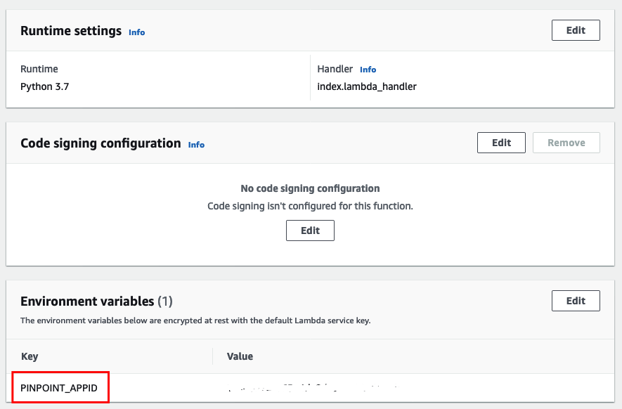
An AWS Lambda function has been created to receive the events. The Lambda function uses Python and Boto3 to read the records delivered by Kinesis Data Streams. It then performs the update_endpoint API calls in order to add, update, or delete endpoints in the Amazon Pinpoint application.

Lambda code and configuration is accessible through the Lambda Functions Console. In order to inspect the Python code, click the Functions item on the left side. Select the function starting with pinpointblogstack-MainStack by clicking on the function name.

Note: The PINPOINT_APPID under the Environment variables section. This variable provides the Lambda function with the Amazon Pinpoint application ID to make the API call.

LambdaPPAPPID

Inspect Amazon Pinpoint Application in Amazon Pinpoint Console

A Pinpoint application is needed by the Lambda Function to update the endpoints. This application has been created with an SMS Channel by the CloudFormation template. Once the data from the RDS database has been imported into Pinpoint as SMS endpoints, you can validate this import by creating a segment in Pinpoint.

PinpointProject

Testing

With the Lambda function ready, you now test the whole solution.

  1. To initiate the end-to-end test, go to the Cloud9 terminal. Perform the following SQL statement on the optin_table:
    UPDATE optin_status SET optin=0 WHERE userid='user1';
    UPDATE optin_status SET optin=0 WHERE userid='user2';
    UPDATE optin_status SET optin=0 WHERE userid='user3';
    UPDATE optin_status SET optin=0 WHERE userid='user4';
  2. This statement will cause four changes in the database which is collected by DMS and passed to Kinesis Data Streams stream.
  3. This triggers the Lambda function that construct an update_endpoint API call to the Amazon Pinpoint application.
  4. The update_endpoint operation is an upsert operation. Therefore, if the endpoint does not exist on the Amazon Pinpoint application, it creates one. Otherwise, it updates the current endpoint.
  5. In the initial dataset, all the opt-in values are 1. Therefore, these endpoints will be created with an OptOut value of NONE in Amazon Pinpoint.
  6. All OptOut=NONE typed endpoints are considered as active endpoints. Therefore, they are available to be used within segments.

Create Amazon Pinpoint Segment

  1. In order to see these changes, go to the Pinpoint console. Click on PinpointBlogApp.
    PinpointConsole
  2. Click on Segments on the left side. Then click Create a segment.
    PinpointSegment
  3. For the segment name, enter US-Segment.
  4. Select Endpoint from the Filter dropdown.
  5. Under the Choose an endpoint attribute dropdown, select Country.
  6. For Choose values enter US.
    Note: As you do this, the right panel Segment estimate will refresh to show the number of endpoints eligible for this segment filter.
  7. Click Create segment at the bottom of the page.
    PinpointSegDetails
  8. Once the new segment is created, you are directed to the newly created segment with configuration details. You should see five eligible endpoints corresponding to database table rows.
    PinpointSegUpdate
  9. Now, change one row by issuing the following SQL statement. This simulates a user opting out from SMS communication for one of their numbers.
    UPDATE optin_status SET optin=0 WHERE userid='user5';
  10. After the update, go to the Amazon Pinpoint console. Check the eligible endpoints again. You should only see four eligible endpoints.

PinpointSegUpdate

Cleanup

If you no longer want to incur further charge, delete the Cloudformation stack named pinpointblogstack. Select it and click Delete.

PinpointCleanup

Conclusion

This solution walks you through how opt-in change events are delivered from Amazon RDS to Amazon Pinpoint. You can use this solution in other use cases as well. Some examples are importing segments from a 3rd party application like Salesforce and importing other types of channels like e-mail, push, and voice. To learn more about Amazon Pinpoint, visit our website.

Architecting a Data Lake for Higher Education Student Analytics

Post Syndicated from Craig Jordan original https://aws.amazon.com/blogs/architecture/architecting-data-lake-for-higher-education-student-analytics/

One of the keys to identifying timely and impactful actions is having enough raw material to work with. However, this up-to-date information typically lives in the databases that sit behind several different applications. One of the first steps to finding data-driven insights is gathering that information into a single store that an analyst can use without interfering with those applications.

For years, reporting environments have relied on a data warehouse stored in a single, separate relational database management system (RDBMS). But now, due to the growing use of Software as a service (SaaS) applications and NoSQL database options, data may be stored outside the data center and in formats other than tables of rows and columns. It’s increasingly difficult to access the data these applications maintain, and a data warehouse may not be flexible enough to house the gathered information.

For these reasons, reporting teams are building data lakes, and those responsible for using data analytics at universities and colleges are no different. However, it can be challenging to know exactly how to start building this expanded data repository so it can be ready to use quickly and still expandable as future requirements are uncovered. Helping higher education institutions address these challenges is the topic of this post.

About Maryville University

Maryville University is a nationally recognized private institution located in St. Louis, Missouri, and was recently named the second fastest growing private university by The Chronicle of Higher Education. Even with its enrollment growth, the university is committed to a highly personalized education for each student, which requires reliable data that is readily available to multiple departments. University leaders want to offer the right help at the right time to students who may be having difficulty completing the first semester of their course of study. To get started, the data experts in the Office of Strategic Information and members of the IT Department needed to create a data environment to identify students needing assistance.

Critical data sources

Like most universities, Maryville’s student-related data centers around two significant sources: the student information system (SIS), which houses student profiles, course completion, and financial aid information; and the learning management system (LMS) in which students review course materials, complete assignments, and engage in online discussions with faculty and fellow students.

The first of these, the SIS, stores its data in an on-premises relational database, and for several years, a significant subset of its contents had been incorporated into the university’s data warehouse. The LMS, however, contains data that the team had not tried to bring into their data warehouse. Moreover, that data is managed by a SaaS application from Instructure, called “Canvas,” and is not directly accessible for traditional extract, transform, and load (ETL) processing. The team recognized they needed a new approach and began down the path of creating a data lake in AWS to support their analysis goals.

Getting started on the data lake

The first step the team took in building their data lake made use of an open source solution that Harvard’s IT department developed. The solution, comprised of AWS Lambda functions and Amazon Simple Storage Service (S3) buckets, is deployed using AWS CloudFormation. It enables any university that uses Canvas for their LMS to implement a solution that moves LMS data into an S3 data lake on a daily basis. The following diagram illustrates this portion of Maryville’s data lake architecture:

The data lake for the Learning Management System data

Diagram 1: The data lake for the Learning Management System data

The AWS Lambda functions invoke the LMS REST API on a daily schedule resulting in Maryville’s data, which has been previously unloaded and compressed by Canvas, to be securely stored into S3 objects. AWS Glue tables are defined to provide access to these S3 objects. Amazon Simple Notification Service (SNS) informs stakeholders the status of the data loads.

Expanding the data lake

The next step was deciding how to copy the SIS data into S3. The team decided to use the AWS Database Migration Service (DMS) to create daily snapshots of more than 2,500 tables from this database. DMS uses a source endpoint for secure access to the on-premises database instance over VPN. A target endpoint determines the specific S3 bucket into which the data should be written. A migration task defines which tables to copy from the source database along with other migration options. Finally, a replication instance, a fully managed virtual machine, runs the migration task to copy the data. With this configuration in place, the data lake architecture for SIS data looks like this:

Diagram 2: Migrating data from the Student Information System

Diagram 2: Migrating data from the Student Information System

Handling sensitive data

In building a data lake you have several options for handling sensitive data including:

  • Leaving it behind in the source system and avoid copying it through the data replication process
  • Copying it into the data lake, but taking precautions to ensure that access to it is limited to authorized staff
  • Copying it into the data lake, but applying processes to eliminate, mask, or otherwise obfuscate the data before it is made accessible to analysts and data scientists

The Maryville team decided to take the first of these approaches. Building the data lake gave them a natural opportunity to assess where this data was stored in the source system and then make changes to the source database itself to limit the number of highly sensitive data fields.

Validating the data lake

With these steps completed, the team turned to the final task, which was to validate the data lake. For this process they chose to make use of Amazon Athena, AWS Glue, and Amazon Redshift. AWS Glue provided multiple capabilities including metadata extraction, ETL, and data orchestration. Metadata extraction, completed by Glue crawlers, quickly converted the information that DMS wrote to S3 into metadata defined in the Glue data catalog. This enabled the data in S3 to be accessed using standard SQL statements interactively in Athena. Without the added cost and complexity of a database, Maryville’s data analyst was able to confirm that the data loads were completing successfully. He was also able to resolve specific issues encountered on particular tables. The SQL queries, written in Athena, could later be converted to ETL jobs in AWS Glue, where they could be triggered on a schedule to create additional data in S3. Athena and Glue enabled the ETL that was needed to transform the raw data delivered to S3 into prepared datasets necessary for existing dashboards.

Once curated datasets were created and stored in S3, the data was loaded into an AWS Redshift data warehouse, which supported direct access by tools outside of AWS using ODBC/JDBC drivers. This capability enabled Maryville’s team to further validate the data by attaching the data in Redshift to existing dashboards that were running in Maryville’s own data center. Redshift’s stored procedure language allowed the team to port some key ETL logic so that the engineering of these datasets could follow a process similar to approaches used in Maryville’s on-premises data warehouse environment.

Conclusion

The overall data lake/data warehouse architecture that the Maryville team constructed currently looks like this:

The complete architecture

Diagram 3: The complete architecture

Through this approach, Maryville’s two-person team has moved key data into position for use in a variety of workloads. The data in S3 is now readily accessible for ad hoc interactive SQL workloads in Athena, ETL jobs in Glue, and ultimately for machine learning workloads running in EC2, Lambda or Amazon Sagemaker. In addition, the S3 storage layer is easy to expand without interrupting prior workloads. At the time of this writing, the Maryville team is both beginning to use this environment for machine learning models described earlier as well as adding other data sources into the S3 layer.

Acknowledgements

The solution described in this post resulted from the collaborative effort of Christine McQuie, Data Engineer, and Josh Tepen, Cloud Engineer, at Maryville University, with guidance from Travis Berkley and Craig Jordan, AWS Solutions Architects.

Apply record level changes from relational databases to Amazon S3 data lake using Apache Hudi on Amazon EMR and AWS Database Migration Service

Post Syndicated from Ninad Phatak original https://aws.amazon.com/blogs/big-data/apply-record-level-changes-from-relational-databases-to-amazon-s3-data-lake-using-apache-hudi-on-amazon-emr-and-aws-database-migration-service/

Data lakes give organizations the ability to harness data from multiple sources in less time. Users across different roles are now empowered to collaborate and analyze data in different ways, leading to better, faster decision-making. Amazon Simple Storage Service (Amazon S3) is the highly performant object storage service for structured and unstructured data and the storage service of choice to build a data lake.

However, many use cases like performing change data capture (CDC) from an upstream relational database to an Amazon S3-based data lake require handling data at a record level. Performing an operation like inserting, updating, and deleting individual records from a dataset requires the processing engine to read all the objects (files), make the changes, and rewrite the entire dataset as new files. Furthermore, making the data available in the data lake in near-real time often leads to the data being fragmented over many small files, resulting in poor query performance. Apache Hudi is an open-source data management framework that enables you to manage data at the record level in Amazon S3 data lakes, thereby simplifying building CDC pipelines and making it efficient to do streaming data ingestion. Datasets managed by Hudi are stored in Amazon S3 using open storage formats, and integrations with Presto, Apache Hive, Apache Spark, and the AWS Glue Data Catalog give you near real-time access to updated data using familiar tools. Hudi is supported in Amazon EMR and is automatically installed when you choose Spark, Hive, or Presto when deploying your EMR cluster.

In this post, we show you how to build a CDC pipeline that captures the data from an Amazon Relational Database Service (Amazon RDS) for MySQL database using AWS Database Migration Service (AWS DMS) and applies those changes to a dataset in Amazon S3 using Apache Hudi on Amazon EMR. Apache Hudi includes the utility HoodieDeltaStreamer, which provides an easy way to ingest data from many sources, such as a distributed file system or Kafka. It manages checkpointing, rollback, and recovery so you don’t need to keep track of what data has been read and processed from the source, which makes it easy to consume change data. It also allows for lightweight SQL-based transformations on the data as it is being ingested. For more information, see Writing Hudi Tables. Support for AWS DMS with HoodieDeltaStreamer is provided with Apache Hudi version 0.5.2 and is available on Amazon EMR 5.30.x and 6.1.0.

Architecture overview

The following diagram illustrates the architecture we deploy to build our CDC pipeline.

In this architecture, we have a MySQL instance on Amazon RDS. AWS DMS pulls full and incremental data (using the CDC feature of AWS DMS) into an S3 bucket in Parquet format. HoodieDeltaStreamer on an EMR cluster is used to process the full and incremental data to create a Hudi dataset. As the data in the MySQL database gets updated, the AWS DMS task picks up the changes and takes them to the raw S3 bucket. The HoodieDeltastreamer job can be run on the EMR cluster at a certain frequency or in a continuous mode to apply these changes to the Hudi dataset in the Amazon S3 data lake. You can query this data with tools such as SparkSQL, Presto, Apache Hive running on the EMR cluster, and Amazon Athena.

Deploying the solution resources

We use AWS CloudFormation to deploy these components in your AWS account. Choose an AWS Region for deployment where the following services are available:

You need to meet the following prerequisites before deploying the CloudFormation template:

  • Have a VPC with at least two public subnets in your account.
  • Have a S3 bucket where you want to collect logs from the EMR cluster. This should be in the same AWS region where you spin up the CloudFormation stack.
  • Have an AWS Identity and Access Management (IAM) role dms-vpc-role. For instructions on creating one, see Security in AWS Database Migration Service.
  • If you’re deploying the stack in an account using the AWS Lake Formation permission model, validate the following settings:
    • The IAM user used to deploy the stack is added as a data lake administrator under Lake Formation or the IAM user used to deploy the stack has IAM privileges to create databases in the AWS Glue Data Catalog.
    • The Data Catalog settings under Lake Formation are configured to use only IAM access control for new databases and new tables in new databases. This makes sure that all access to the newly created databases and tables in the Data Catalog are controlled solely using IAM permissions.
  • IAMAllowedPrincipals is granted database creator privilege on the Lake Formation Database creators page.

If this privilege is not in place, grant it by choosing Grant and selecting the Create database permission.

These Lake Formation settings are required so that all permissions to the Data Catalog objects are controlled using IAM only.

Launching the CloudFormation stack

To launch the CloudFormation stack, complete the following steps:

  1. Choose Launch Stack:
  2. Provide the mandatory parameters in the Parameters section, including an S3 bucket to store the Amazon EMR logs and a CIDR IP range from where you want to access Amazon RDS for MySQL.
  3. Follow through the CloudFormation stack creation wizard, leaving rest of the default values unchanged.
  4. On the final page, select I acknowledge that AWS CloudFormation might create IAM resources with custom names.
  5. Choose Create stack.
  6. When the stack creation is complete, record the details of the S3 bucket, EMR cluster, and Amazon RDS for MySQL details on the Outputs tab of the CloudFormation stack.

The CloudFormation template uses m5.xlarge and m5.2xlarge instances for the EMR cluster. If these instance types aren’t available in the Region or Availability Zone you have selected for deployment, the creation of the CloudFormation stack fails. If that happens, choose a Region or subnet where the instance type is available. For more information about working around this issue, see Instance Type Not Supported.

CloudFormation also creates and configures the AWS DMS endpoints and tasks with requisite connection attributes such as dataFormat, timestampColumnName, and parquetTimestampInMillisecond. For more information, see Extra connection attributes when using Amazon S3 as a target for AWS DMS.

The database instance deployed as part of the CloudFormation stack has already been created with the settings needed for AWS DMS to work in CDC mode on the database. These are:

  • binlog_format=ROW
  • binlog_checksum=NONE

Also, automatic backups are enabled on the RDS DB instance. This is a required attribute for AWS DMS to do CDC. For more information, see Using a MySQL-compatible database as a source for AWS DMS.

Running the end-to-end data flow

Now that the CloudFormation stack is deployed, we can run our data flow to get the full and incremental data from MySQL into a Hudi dataset in our data lake.

  1. As a best practice, retain your binlogs for at least 24 hours. Log in to your Amazon RDS for MySQL database using your SQL client and run the following command:
    call mysql.rds_set_configuration('binlog retention hours', 24)

  2. Create a table in the dev database:
    create table dev.retail_transactions(
    tran_id INT,
    tran_date DATE,
    store_id INT,
    store_city varchar(50),
    store_state char(2),
    item_code varchar(50),
    quantity INT,
    total FLOAT);

  3. When the table is created, insert some dummy data into the database:
    insert into dev.retail_transactions values(1,'2019-03-17',1,'CHICAGO','IL','XXXXXX',5,106.25);
    insert into dev.retail_transactions values(2,'2019-03-16',2,'NEW YORK','NY','XXXXXX',6,116.25);
    insert into dev.retail_transactions values(3,'2019-03-15',3,'SPRINGFIELD','IL','XXXXXX',7,126.25);
    insert into dev.retail_transactions values(4,'2019-03-17',4,'SAN FRANCISCO','CA','XXXXXX',8,136.25);
    insert into dev.retail_transactions values(5,'2019-03-11',1,'CHICAGO','IL','XXXXXX',9,146.25);
    insert into dev.retail_transactions values(6,'2019-03-18',1,'CHICAGO','IL','XXXXXX',10,156.25);
    insert into dev.retail_transactions values(7,'2019-03-14',2,'NEW YORK','NY','XXXXXX',11,166.25);
    insert into dev.retail_transactions values(8,'2019-03-11',1,'CHICAGO','IL','XXXXXX',12,176.25);
    insert into dev.retail_transactions values(9,'2019-03-10',4,'SAN FRANCISCO','CA','XXXXXX',13,186.25);
    insert into dev.retail_transactions values(10,'2019-03-13',1,'CHICAGO','IL','XXXXXX',14,196.25);
    insert into dev.retail_transactions values(11,'2019-03-14',5,'CHICAGO','IL','XXXXXX',15,106.25);
    insert into dev.retail_transactions values(12,'2019-03-15',6,'CHICAGO','IL','XXXXXX',16,116.25);
    insert into dev.retail_transactions values(13,'2019-03-16',7,'CHICAGO','IL','XXXXXX',17,126.25);
    insert into dev.retail_transactions values(14,'2019-03-16',7,'CHICAGO','IL','XXXXXX',17,126.25);
    

    We now use AWS DMS to start pushing this data to Amazon S3.

  4. On the AWS DMS console, run the task hudiblogload.

This task does a full load of the table to Amazon S3 and then starts writing incremental data.

If you’re prompted to test the AWS DMS endpoints while starting the AWS DMS task for the first time, you should do so. It’s generally a good practice to test the source and target endpoints before starting an AWS DMS task for the first time.

In a few minutes, the status of the task changes to Load complete, replication ongoing, which means that the full load is complete and the ongoing replication has started. You can go to the S3 bucket created by the stack and you should see a .parquet file under the dmsdata/dev/retail_transactions folder in your S3 bucket.

  1. On the Hardware tab of your EMR cluster, choose the master instance group and note the EC2 instance ID for the master instance.
  2. On the Systems Manager console, choose Session Manager.
  3. Choose Start Session to start a session with the master node of your cluster.

If you face challenges connecting to the master instance of the EMR cluster, see Troubleshooting Session Manager.

  1. Switch the user to Hadoop by running the following command:
    sudo su hadoop

In a real-life use case, the AWS DMS task starts writing incremental files to the same Amazon S3 location when the full load is complete. The way to distinguish full load vs. incremental load files is that the full load files have a name starting with LOAD, whereas CDC filenames have datetimestamps, as you see in a later step. From a processing perspective, we want to process the full load into the Hudi dataset and then start incremental data processing. To do this, we move the full load files to a different S3 folder under the same S3 bucket and process those before we start processing incremental files.

  1. Run the following command on the master node of the EMR cluster (replace <s3-bucket-name> with your actual bucket name):
    aws s3 mv s3://<s3-bucket-name>/dmsdata/dev/retail_transactions/ s3://<s3-bucket-name>/dmsdata/data-full/dev/retail_transactions/  --exclude "*" --include "LOAD*.parquet" --recursive

With the full table dump available in the data-full folder, we now use the HoodieDeltaStreamer utility on the EMR cluster to populate the Hudi dataset on Amazon S3.

  1. Run the following command to populate the Hudi dataset to the hudi folder in the same S3 bucket (replace <s3-bucket-name> with the name of the S3 bucket created by the CloudFormation stack):
    spark-submit --class org.apache.hudi.utilities.deltastreamer.HoodieDeltaStreamer  \
      --packages org.apache.hudi:hudi-utilities-bundle_2.11:0.5.2-incubating,org.apache.spark:spark-avro_2.11:2.4.5 \
      --master yarn --deploy-mode cluster \
    --conf spark.serializer=org.apache.spark.serializer.KryoSerializer \
    --conf spark.sql.hive.convertMetastoreParquet=false \
    /usr/lib/hudi/hudi-utilities-bundle_2.11-0.5.2-incubating.jar \
      --table-type COPY_ON_WRITE \
      --source-ordering-field dms_received_ts \
      --props s3://<s3-bucket-name>/properties/dfs-source-retail-transactions-full.properties \
      --source-class org.apache.hudi.utilities.sources.ParquetDFSSource \
      --target-base-path s3://<s3-bucket-name>/hudi/retail_transactions --target-table hudiblogdb.retail_transactions \
      --transformer-class org.apache.hudi.utilities.transform.SqlQueryBasedTransformer \
        --payload-class org.apache.hudi.payload.AWSDmsAvroPayload \
    --schemaprovider-class org.apache.hudi.utilities.schema.FilebasedSchemaProvider \
      --enable-hive-sync
    

The preceding command runs a Spark job that runs the HoodieDeltaStreamer utility. For more information about the parameters used in this command, see Writing Hudi Tables.

When the Spark job is complete, you can navigate to the AWS Glue console and find a table called retail_transactions created under the hudiblogdb database. The input format for the table is org.apache.hudi.hadoop.HoodieParquetInputFormat.

Next, we query the data and look at the data in the retail_transactions table in the catalog.

  1. In the Systems Manager session established earlier, run the following command (make sure that you have completed all the prerequisites for the post, including adding IAMAllowedPrincipals as a database creator in Lake Formation):
    spark-shell --conf "spark.serializer=org.apache.spark.serializer.KryoSerializer" --conf "spark.sql.hive.convertMetastoreParquet=false" \
    --packages org.apache.hudi:hudi-spark-bundle_2.11:0.5.2-incubating,org.apache.spark:spark-avro_2.11:2.4.5 \
    --jars /usr/lib/hudi/hudi-spark-bundle_2.11-0.5.2-incubating.jar,/usr/lib/spark/external/lib/spark-avro.jar
    

  2. Run the following query on the retail_transactions table:
    spark.sql("Select * from hudiblogdb.retail_transactions order by tran_id").show()

You should see the same data in the table as the MySQL database with a few columns added by the HoodieDeltaStreamer process.

We now run some DML statements on our MySQL database and take these changes through to the Hudi dataset.

  1. Run the following DML statements on the MySQL database:
    insert into dev.retail_transactions values(15,'2019-03-16',7,'CHICAGO','IL','XXXXXX',17,126.25);
    update dev.retail_transactions set store_city='SPRINGFIELD' where tran_id=12;
    delete from dev.retail_transactions where tran_id=2;

In a few minutes, you see a new .parquet file created under dmsdata/dev/retail_transactions folder in the S3 bucket.

  1. Run the following command on the EMR cluster to get the incremental data to the Hudi dataset (replace <s3-bucket-name> with the name of the S3 bucket created by the CloudFormation template):
    spark-submit --class org.apache.hudi.utilities.deltastreamer.HoodieDeltaStreamer  \
      --packages org.apache.hudi:hudi-utilities-bundle_2.11:0.5.2-incubating,org.apache.spark:spark-avro_2.11:2.4.5 \
      --master yarn --deploy-mode cluster \
    --conf spark.serializer=org.apache.spark.serializer.KryoSerializer \
    --conf spark.sql.hive.convertMetastoreParquet=false \
    /usr/lib/hudi/hudi-utilities-bundle_2.11-0.5.2-incubating.jar \
      --table-type COPY_ON_WRITE \
      --source-ordering-field dms_received_ts \
      --props s3://<s3-bucket-name>/properties/dfs-source-retail-transactions-incremental.properties \
      --source-class org.apache.hudi.utilities.sources.ParquetDFSSource \
      --target-base-path s3://<s3-bucket-name>/hudi/retail_transactions --target-table hudiblogdb.retail_transactions \
      --transformer-class org.apache.hudi.utilities.transform.SqlQueryBasedTransformer \
        --payload-class org.apache.hudi.payload.AWSDmsAvroPayload \
    --schemaprovider-class org.apache.hudi.utilities.schema.FilebasedSchemaProvider \
      --enable-hive-sync \
    --checkpoint 0

The key difference between this command and the previous one is in the properties file that was used as an argument to the –-props and --checkpoint parameters. For the earlier command that performed the full load, we used dfs-source-retail-transactions-full.properties; for the incremental one, we used dfs-source-retail-transactions-incremental.properties. The differences between these two property files are:

  • The location of source data changes between full and incremental data in Amazon S3.
  • The SQL transformer query included a hard-coded Op field for the full load task, because an AWS DMS first-time full load doesn’t include the Op field for Parquet datasets. The Op field can have values of I, U, and D—for Insert, Update and Delete indicators.

We cover the details of the --checkpoint parameter in the Considerations when deploying to production section later in this post.

  1. When the job is complete, run the same query in spark-shell.

You should see these updates applied to the Hudi dataset.

You can use the Hudi CLI to administer Hudi datasets to view information about commits, the filesystem, statistics, and more.

  1. To do this, in the Systems Manager session, run the following command:
    /usr/lib/hudi/cli/bin/hudi-cli.sh

  2. Inside the Hudi-cli, run the following command (replace the <s3-bucket-name> with the S3 bucket created by the Cloud Formation stack):
    connect --path s3://<s3-bucket-name>/hudi/retail_transactions

  3. To inspect commits on your Hudi dataset, run the following command:
    commits show

You can also query incremental data from the Hudi dataset. This is particularly useful when you want to take incremental data for downstream processing like aggregations. Hudi provides multiple ways of pulling data incrementally which is documented here. An example of how to use this feature is available in the Hudi Quick Start Guide.

Considerations when deploying to production

The preceding setup showed an example of how to build a CDC pipeline from your relational database to your Amazon S3-based data lake. However, if you want to use this solution for production, you should consider the following:

  • To ensure high availability, you can set up the AWS DMS instance in a Multi-AZ configuration.
  • The CloudFormation stack deployed the required properties files needed by the deltastreamer utility into the S3 bucket at s3://<s3-bucket-name>/properties/. You may need to customize these based on your requirements. For more information, see Configurations. There are a few parameters that may need your attention:
    • deltastreamer.transformer.sql – This property exposes an extremely powerful feature of the deltastreamer utility: it enables you to transform data on the fly as it’s being ingested and persisted in the Hudi dataset. In this post, we have shown a basic transformation that casts the tran_date column to a string, but you can apply any transformation as part of this query.
    • parquet.small.file.limit – This field is in bytes and a critical storage configuration specifying how Hudi handles small files on Amazon S3. Small files can happen due to the number of records being processed in each insert per partition. Setting this value allows Hudi to continue to treat inserts in a particular partition as updates to the existing files, causing files that are up to the size of this small.file.limit to be rewritten and keep growing in size.
    • parquet.max.file.size – This is the max file size of a single Parquet in your Hudi dataset, after which a new file is created to store more data. For Amazon S3 storage and data querying needs, we can keep this around 256 MB–1 GB (256x1024x1024 = 268435456).
    • [Insert|Upsert|bulkinsert].shuffle.parallelism – In this post, we dealt with a small dataset of few records only. However, in real-life situations, you might want to bring in hundreds of millions of records in the first load, and then incremental CDC can potentially be in millions per day. There is a very important parameter to set when you want quite predictable control on the number of files in each of your Hudi dataset partitions. This is also needed to ensure you don’t hit an Apache Spark limit of 2 GB for data shuffle blocks when processing large amounts of data. For example, if you plan to load 200 GBs of data in first load and want to keep file sizes of approximately 256 MB, set the shuffle parallelism parameters for this dataset as 800 (200×1024/256). For more information, see Tuning Guide.
  • In the incremental load deltastreamer command, we used an additional parameter: --checkpoint 0. When deltastreamer writes a Hudi dataset, it persists checkpoint information in the .commit files under the .hoodie folder. It uses this information in subsequent runs and only reads that data from Amazon S3, which is created after this checkpoint time. In a production scenario, after you start the AWS DMS task, the task keeps writing incremental data to the target S3 folder as soon as the full load is complete. In the steps that we followed, we ran a command on the EMR cluster to manually move the full load files to another folder and process the data from there. When we did that, the timestamp associated with the S3 objects changes to the most current timestamp. If we run the incremental load without the checkpoint argument, deltastreamer doesn’t pick up any incremental data written to Amazon S3 before we manually moved the full load files. To make sure that all incremental data is processed by deltastreamer the first time, set the checkpoint to 0, which makes it process all incremental data in the folder. However, only use this parameter for the first incremental load and let deltastreamer use its own checkpointing methodology from that point onwards.
  • For this post, we ran the spark-submit command manually. However, in production, you can run it as a step on the EMR cluster.
  • You can either schedule the incremental data load command to run at a regular interval using a scheduling or orchestration tool, or run it in a continuous fashion at a certain frequency by passing additional parameters to the spark-submit command --min-sync-interval-seconds XX –continuous, where XX is the number of seconds between each run of the data pull. For example, if you want to run the processing every 5 minutes, replace XX with 300.

Cleaning up

When you are done exploring the solution, complete the following steps to clean up the resources deployed by CloudFormation:

  1. Empty the S3 bucket created by the CloudFormation stack
  2. Delete any Amazon EMR log files generated under s3://<EMR-Logs-S3-Bucket> /HudiBlogEMRLogs/.
  3. Stop the AWS DMS task Hudiblogload.
  4. Delete the CloudFormation stack.
  5. Delete any Amazon RDS for MySQL database snapshots retained after the CloudFormation template is deleted.

Conclusion

More and more data lakes are being built on Amazon S3, and these data lakes often need to be hydrated with change data from transactional systems. Handling deletes and upserts of data into the data lake using traditional methods involves a lot of heavy lifting. In this post, we saw how to easily build a solution with AWS DMS and HoodieDeltaStreamer on Amazon EMR. We also looked at how to perform lightweight record-level transformations when integrating data into the data lake, and how to use this data for downstream processes like aggregations. We also discussed the important settings and command line options that were used and how you could modify them to suit your requirements.


About the Authors

Ninad Phatak is a Senior Analytics Specialist Solutions Architect with Amazon Internet Services Private Limited. He specializes in data engineering and datawarehousing technologies and helps customers architect their analytics use cases and platforms on AWS.


Raghu Dubey is a Senior Analytics Specialist Solutions Architect with Amazon Internet Services Private Limited. He specializes in Big Data Analytics, Data warehousing and BI and helps customers build scalable data analytics platforms.
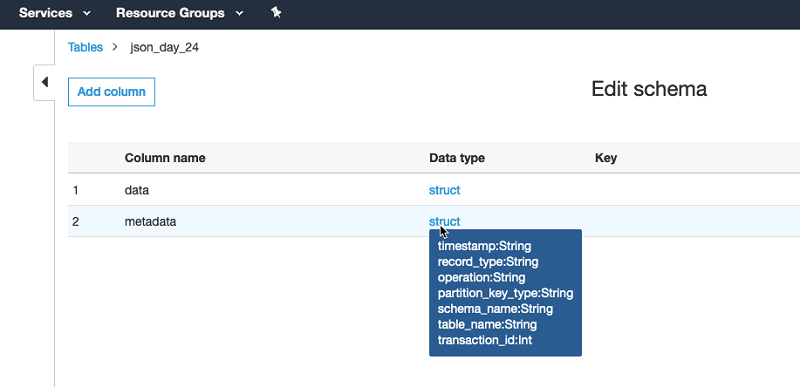
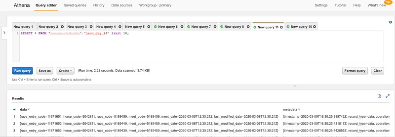


Stream CDC into an Amazon S3 data lake in Parquet format with AWS DMS

Post Syndicated from Viral Shah original https://aws.amazon.com/blogs/big-data/stream-cdc-into-an-amazon-s3-data-lake-in-parquet-format-with-aws-dms/

Most organizations generate data in real time and ever-increasing volumes. Data is captured from a variety of sources, such as transactional and reporting databases, application logs, customer-facing websites, and external feeds. Companies want to capture, transform, and analyze this time-sensitive data to improve customer experiences, increase efficiency, and drive innovations. With increased data volume and velocity, it’s imperative to capture the data from source systems as soon as they are generated and store them on a secure, scalable, and cost-efficient platform.

AWS Database Migration Service (AWS DMS) performs continuous data replication using change data capture (CDC). Using CDC, you can determine and track data that has changed and provide it as a stream of changes that a downstream application can consume and act on. Most database management systems manage a transaction log that records changes made to the database contents and metadata. AWS DMS reads the transaction log by using engine-specific API operations and functions and captures the changes made to the database in a nonintrusive manner.

Amazon Simple Storage Service (Amazon S3) is the largest and most performant object storage service for structured and unstructured data and the storage service of choice to build a data lake. With Amazon S3, you can cost-effectively build and scale a data lake of any size in a secure environment where data is protected by 99.999999999% of durability.

AWS DMS offers many options to capture data changes from relational databases and store the data in columnar format (Apache Parquet) into Amazon S3:

The second option helps you build a flexible data pipeline to ingest data into an Amazon S3 data lake from several relational and non-relational data sources, compared to just relational data sources support in the former option. Kinesis Data Firehose provides pre-built AWS Lambda blueprints for converting common data sources such as Apache logs and system logs to JSON and CSV formats or writing your own custom functions. It can also convert the format of incoming data from JSON to Parquet or Apache ORC before storing the data in Amazon S3. Data stored in columnar format gives you faster and lower-cost queries with downstream analytics services like Amazon Athena.

In this post, we focus on the technical challenges outlined in the second option and how to address them.

As shown in the following reference architecture, data is ingested from a database into Parquet format in Amazon S3 via AWS DMS integrating with Kinesis Data Streams and Kinesis Data Firehose.

Our solution provides flexibility to ingest data from several sources using Kinesis Data Streams and Kinesis Data Firehose with built-in data format conversion and integrated data transformation capabilities before storing data in a data lake. For more information about data ingestion into Kinesis Data Streams, see Writing Data into Amazon Kinesis Data Streams. You can then query Parquet data in Amazon S3 efficiently with Athena.

Implementing the architecture

AWS DMS can migrate data to and from most widely used commercial and open-source databases. You can migrate and replicate data directly to Amazon S3 in CSV and Parquet formats, and store data in Amazon S3 in Parquet because it offers efficient compression and encoding schemes. Parquet format allows compression schemes on a per-column level, and is future-proofed to allow adding more encodings as they are invented and implemented.

AWS DMS supports Kinesis Data Streams as a target. Kinesis Data Streams is a massively scalable and durable real-time data streaming service that can collect and process large streams of data records in real time. AWS DMS service publishes records to a data stream using JSON. For more information about configuration details, see Use the AWS Database Migration Service to Stream Change Data to Amazon Kinesis Data Streams.

Kinesis Data Firehose can pull data from Kinesis Data Streams. It’s a fully managed service that delivers real-time streaming data to destinations such as Amazon S3, Amazon Redshift, Amazon Elasticsearch Service (Amazon ES), and Splunk. Kinesis Data Firehose can convert the format of input data from JSON to Parquet or ORC before sending it to Amazon S3. It needs reference schema to interpret the AWS DMS streaming data in JSON and convert into Parquet. In this post, we use AWS Glue, a fully managed ETL service, to create a schema in the AWS Glue Data Catalog for Kinesis Data Firehose to reference.

When AWS DMS migrates records, it creates additional fields (metadata) for each migrated record. The metadata provides additional information about the record being migrated, such as source table name, schema name, and type of operation. Most metadata fields add – in their field names (for example, record-type, schema-name, table-name, transaction-id). See the following code:

{
        "data": {
            "MEET_CODE": 5189459,
            "MEET_DATE": "2020-02-21T19:20:04Z",
            "RACE_CODE": 5189459,
            "LAST_MODIFIED_DATE": "2020-02-24T19:20:04Z",
            "RACE_ENTRY_CODE": 11671651,
            "HORSE_CODE": 5042811
        },
        "metadata": {
            "transaction-id": 917505,
            "schema-name": "SH",
            "operation": "insert",
            "table-name": "RACE_ENTRY",
            "record-type": "data",
            "timestamp": "2020-02-26T00:20:07.482592Z",
            "partition-key-type": "schema-table"
        }
    }

Additional metadata added by AWS DMS leads to an error during the data format conversion phase in Kinesis Data Firehose. Kinesis Data Firehose follows Hive style formatting and therefore doesn’t recognize the – character in the metadata field names during data conversion from JSON into Parquet and returns an error message: expected at the position 30 of ‘struct’ but ‘-’ is found. For example, see the following code:

{
	"deliveryStreamARN": "arn:aws:firehose:us-east-1:1234567890:deliverystream/abc-def-KDF",
	"destination": "arn:aws:s3:::abc-streaming-bucket",
	"deliveryStreamVersionId": 13,
	"message": "The schema is invalid. Error parsing the schema:
	 Error: : expected at the position 30 of 'struct<timestamp:string,record-type:string,operation:string,partition-key-type:string,schema-name:string,table-name:string,transaction-id:int>' but '-' is found.",
	"errorCode": "DataFormatConversion.InvalidSchema"
}

You can resolve the issue by making the following changes: specifying JSON key mappings and creating a reference table in AWS Glue before configuring Kinesis Data Firehose.

Specifying JSON key mappings

In your Kinesis Data Firehose configuration, specify JSON key mappings for fields with – in their names. Mapping transforms these specific metadata fields names to _ (for example, record-type changes to record_type).

Use AWS Command Line Interface (AWS CLI) to create Kinesis Data Firehose with the JSON key mappings. Modify the parameters to meet your specific requirements.

Kinesis Data Firehose configuration mapping is only possible through the AWS CLI or API and not through the AWS Management Console.

The following code configures Kinesis Data Firehose with five columns with – in their field names mapped to new field names with _”:

"S3BackupMode": "Disabled",
                    "DataFormatConversionConfiguration": {
                        "SchemaConfiguration": {
                            "RoleARN": "arn:aws:iam::123456789012:role/sample-firehose-delivery-role",
                            "DatabaseName": "sample-db",
                            "TableName": "sample-table",
                            "Region": "us-east-1",
                            "VersionId": "LATEST"
                        },
                        "InputFormatConfiguration": {
                            "Deserializer": {
                                "OpenXJsonSerDe": {
                                "ColumnToJsonKeyMappings":
                                {
                                 "record_type": "record-type","partition_key_type": "partition-key-type","schema_name":"schema-name","table_name":"table-name","transaction_id":"transaction-id"
                                }
                                }

Creating a reference table in AWS Glue

Because Kinesis Data Firehose uses the Data Catalog to reference schema for Parquet format conversion, you must first create a reference table in AWS Glue before configuring Kinesis Data Firehose. Use Athena to create a Data Catalog table. For instructions, see CREATE TABLE. In the table, make sure that the column name uses _ in their names, and manually modify it in advance through the Edit schema option for the referenced table in AWS Glue, if needed.

Use Athena to query the results of data ingested by Kinesis Data Firehose into Amazon S3.

This solution is only applicable in the following use cases:

  • Capturing data changes from your source with AWS DMS
  • Converting data into Parquet with Kinesis Data Firehose

If you want to store data in non-Parquet format (such CSV or JSON) or ingest into Kinesis through other routes, then you don’t need to modify your Kinesis Data Firehose configuration.

Conclusion

This post demonstrated how to convert AWS DMS data into Parquet format and specific configurations to make sure metadata follows the expected format of Kinesis Data Streams and Kinesis Data Firehose. We encourage you to try this solution and take advantage of all the benefits of using AWS DMS with Kinesis Data Streams and Kinesis Data Firehose. For more information, see Getting started with AWS Database Migration Service and Setting up Amazon Kinesis Firehose.

If you have questions or suggestions, please leave a comment.


About the Author

Viral Shah is a Data Lab Architect with Amazon Web Services. Viral helps our customers architect and build data and analytics prototypes in just four days in the AWS Data Lab. He has over 20 years of experience working with enterprise customers and startups primarily in the Data and Database space.