During Security Week 2025, we launched the industry’s first cloud-nativepost-quantum Secure Web Gateway (SWG) and Zero Trust solution, a major step towards securing enterprise network traffic sent from end user devices to public and private networks.
But this is only part of the equation. To truly secure the future of enterprise networking, you need a complete Secure Access Service Edge (SASE).
Today, we complete the equation: Cloudflare One is the first SASE platform to support modern standards-compliant post-quantum (PQ) encryption in our Secure Web Gateway, and across Zero Trust and Wide Area Network (WAN) use cases. More specifically, Cloudflare One now offers post-quantum hybrid ML-KEM (Module-Lattice-based Key-Encapsulation Mechanism) across all major on-ramps and off-ramps.
To complete the equation, we added support for post-quantum encryption to our Cloudflare IPsec (our cloud-native WAN-as-a-Service) and Cloudflare One Appliance (our physical or virtual WAN appliance that establish Cloudflare IPsec connections). Cloudflare IPsec uses the IPsec protocol to establish encrypted tunnels from a customer’s network to Cloudflare’s global network, while IP Anycast is used to automatically route that tunnel to the nearest Cloudflare data center. Cloudflare IPsec simplifies configuration and provides high availability; if a specific data center becomes unavailable, traffic is automatically rerouted to the closest healthy data center. Cloudflare IPsec runs at the scale of our global network, and supports site-to-site across a WAN as well as outbound connections to the Internet.
Quantum threats are not a “next decade” problem. Here is why our customers are prioritizing post-quantum cryptography (PQC) today:
The deadline is approaching. At the end of 2024, the National Institute of Standards and Technology (NIST) sent a clear signal (that has been echoed by other agencies): the era of classical public-key cryptography is coming to an end. NIST set a 2030 deadline for depreciating RSA and Elliptic Curve Cryptography (ECC) and transitioning to PQC that cannot be broken by powerful quantum computers. Organizations that haven’t begun their migration risk being out of compliance and vulnerable as the deadline nears.
Upgrades have historically been tricky. While 2030 might seem far away, upgrading cryptographic algorithms is notoriously difficult. History has shown us that depreciating cryptography can take decades: we found examples of MD5 causing problems 20 years after it was deprecated. This lack of crypto agility — the ability to easily swap out cryptographic algorithms — is a major bottleneck. By integrating PQ encryption directly into Cloudflare One, our SASE platform, we provide built-in crypto agility, simplifying how organizations offer remote access and site-to-site connectivity.
Data may already be at risk. Finally, “Harvest Now, Decrypt Later” is a present and persistent threat, where attackers harvest sensitive network traffic today and then store it until quantum computers become powerful enough to decrypt it. If your data has a shelf life of more than a few years (e.g. financial information, health data, state secrets) it is already at risk unless it is protected by PQ encryption.
The two migrations on the road to quantum safety: key agreement and digital signatures
Transitioning network traffic to post-quantum cryptography (PQC) requires an overhaul of two cryptographic primitives: key agreement and digital signatures.
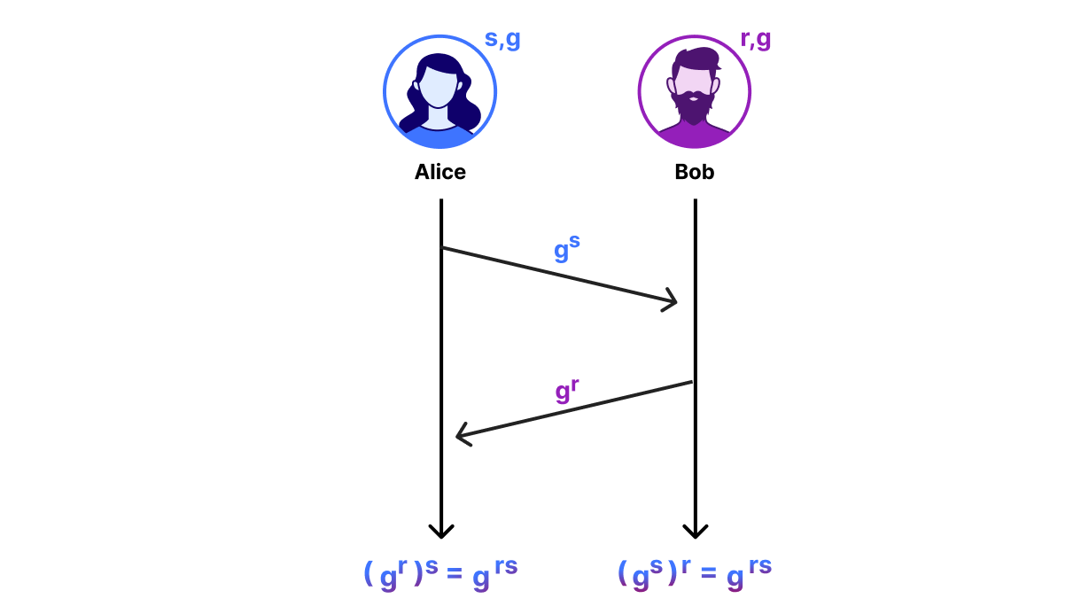
Migration 1: Key establishment. Key agreement allows two parties to establish a shared secret over an insecure channel; the shared secret is then used to encrypt network traffic, resulting in post-quantum encryption. The industry has largely converged on ML-KEM (Module-Lattice-based Key-Encapsulation Mechanism) as the standard PQ key agreement protocol.
ML-KEM has been widely adopted for use in TLS, usually deployed alongside classical Elliptic Curve Diffie Hellman (ECDHE), where the key used to encrypt network traffic is derived by mixing the outputs of the ML-KEM and ECDHE key agreements. (This is also known as “hybrid ML-KEM”). Well over 60% of human-generated TLS traffic to Cloudflare’s network is currently protected with hybrid ML-KEM. The transition to hybrid ML-KEM has been successful because it:
stops “harvest-now, decrypt-later” attacks
does not require specialized hardware or specialized physical connectivity between client and server, unlike approaches like Quantum Key Distribution (QKD)
Because ML-KEM runs in parallel with classical ECDHE, there is no reduction in security and compliance as compared to the classical ECDHE approach.
Migration 2: Digital signatures. Meanwhile, digital signatures and certificates protect authenticity, stopping active adversaries from impersonating the server to the client. Unfortunately, PQ signatures are currently larger in size than classical ECC algorithms, which has slowed their adoption. Fortunately, the migration to PQ signatures is less urgent, because PQ signatures are designed to stop active adversaries armed with powerful quantum computers, which are not known to exist yet. Thus, while Cloudflare is actively contributing to the standardization and rollout of PQ digital signatures, the current Cloudflare IPsec upgrade focuses on upgrading key establishment to hybrid ML-KEM.
The U.S. Cybersecurity & Infrastructure Security Agency (CISA) recognized the nature of these two migrations in its January 2026 publication, “Product Categories for Technologies That Use Post-Quantum Cryptography Standards.”
Breaking new ground with IPsec
To achieve a SASE fully protected with post-quantum encryption, we’ve upgraded our Cloudflare IPsec products to support hybrid ML-KEM in the IPsec protocol.
The IPsec community’s journey toward post-quantum cryptography has been very different from that of TLS. TLS is the de facto standard for encrypting public Internet traffic at Layer 4 — e.g. from a browser to a content delivery network (CDN) — so security and vendor interoperability are at the forefront of its design. Meanwhile, IPsec is a Layer 3 protocol that commonly connects devices built by the same vendor (e.g. two routers), so interoperability has historically been less of a concern. With this in mind, let’s take a look at IPsec’s journey into the quantum future.
Pre-Shared Keys? Quantum key distribution?
RFC 8784, published in May 2020, was intended to be the post-quantum update to IPsec Internet Key Exchange v2 (IKEv2), which is used to establish the symmetric keys used to encrypt IPsec network traffic. RFC 8784 implies the use of either long-lived pre-shared keys (PSK) or quantum key distribution (QKD). Neither of these approaches are very palatable.
RFC 8784 proposes mixing a PSK with a key derived from Diffie Hellman Exchange (DHE), essentially running PSK in hybrid with DHE. This approach protects against harvest-now-decrypt-later attackers, but does not offer forward secrecy against quantum adversaries.
Forward secrecy is a standard desideratum of key agreement protocols. It ensures that a system is secure even if the long-lived key is leaked. The PSK approach in RFC 8784 is vulnerable to an harvest-now-decrypt-later adversary that also obtains a copy of a long-lived PSK, and can then decrypt traffic in the future (by breaking the DHE key agreement) once powerful quantum computers become available.
To solve this forward secrecy issue, RFC 8784 can instead be used to mix the key from the classical DHE with a freshly generated key derived from a QKD protocol.
QKD uses quantum mechanics to establish a shared, secret cryptographic key between two parties. Importantly, for QKD to work, the parties must have specialized hardware or be connected by a dedicated physical connection. This is a significant limitation, rendering QKD useless for common Internet use cases like connecting a laptop to a distant server over Wi-Fi. These limitations are also why we never invested in deploying QKD for Cloudflare IPsec. The U.S. National Security Agency (NSA), Germany’s BSI and the UK National Cyber Security Centre have also warned against relying solely on QKD.
But what about interoperability?
RFC 9370 landed in May 2023, specifying the use of hybrid key agreement rather than PSK or QKD. But unlike TLS, which only supports using post-quantum ML-KEM in parallel with classical DHE, this IPsec standard allows using up to seven different key agreements to run at the same time in parallel with classical Diffie Helman. Moreover, it doesn’t specify details about what these key agreements should be, leaving it up to the vendors to choose their algorithms and implementations. Palo Alto Networks, for example, took this seriously and built support for over seven different PQC ciphersuites into its next generation firewall (NGFW), most of which do not interoperate with other vendors and some of which have not yet been standardized by NIST.
Over the years, TLS has gone in the opposite direction, reducing the number of registered ciphersuites from hundreds in TLS 1.2, down to around five in TLS 1.3. This philosophy of reducing “ciphersuite bloat” is also in line with NIST’s SP 800 52 from 2019. The rationale for reducing “ciphersuite bloat” includes:
Improved interoperability across vendors and regions
Lower risk of attacks that exploit downgrades to weak ciphersuites
Lower risk of security problems due to misconfiguration
Lower risk of implementation flaws by reducing the size of the codebase
This is why we didn’t initially build support for RFC 9370.
Standards that are finally on the right track
It’s also why we were excited when the IPsec community put forth draft-ietf-ipsecme-ikev2-mlkem. This Internet-Draft standardizes PQ exchange for IPsec in the same way PQ key exchange has been widely deployed for TLS: hybrid ML-KEM. The new draft fills in the gaps in RFC 9370, by specifying how to run the ML-KEM as the additional key exchange in parallel with classical Diffie Hellman in IKEv2.
Now that this specification is available, we’ve moved forward with supporting post-quantum IPsec in our Cloudflare IPsec products.
Cloudflare IPsec goes post-quantum
Cloudflare IPsec is a WAN Network-as-a-Service solution that replaces legacy private network architectures by connecting data centers, branch offices, and cloud VPCs to Cloudflare’s global IP Anycast network.
With Cloudflare IPsec, Cloudflare’s network acts as the IKEv2 Responder, awaiting connection requests from an IPsec initiator, which is a branch connector device in the customer’s network. Cloudflare IPsec supports IPsec sessions initiated by branch connectors that include our own Cloudflare One Appliance, along with branch connectors from a diverse set of vendors, including Cisco, Juniper, Palo Alto Networks, Fortinet, Aruba and others.
We’ve implemented production hybrid ML-KEM support in the Cloudflare IPsec IKEv2 Responder, as specified in draft-ietf-ipsecme-ikev2-mlkem. The draft requires a first key exchange to run using a classical Diffie Helman key exchange. The derived key is used to encrypt a second key exchange that is run using ML-KEM. Finally, the keys derived by the two exchanges are mixed and the result is used to secure the data plane traffic in IPsec ESP (Encapsulating Security Payload) mode. ESP mode uses symmetric cryptography and is thus already quantum safe without any additional upgrades. We’ve tested our implementation against the IPsec Initiator in the strongswan reference implementation.
You can see the ciphersuite used in the IKEv2 negotiation by viewing the Cloudflare IPsec logs.
We chose to implement hybrid ML-KEM rather than “pure” ML-KEM, i.e. only ML-KEM without DHE running in parallel, for two reasons. First, we’ve used hybrid ML-KEM across all of our other Cloudflare products, since this is the approach adopted across the TLS community. And second, it provides a “belt-and-suspenders” security: ML-KEM provides protection against quantum harvest-now-decrypt-later attacks, while DHE provides a tried-and-true algorithm against non-quantum adversaries.
An invitation for interoperability
The full value of this implementation can be realized only via interoperability. For this reason, we are inviting other vendors that are building out support for IPsec Initiators in their branch connectors per draft-ietf-ipsecme-ikev2-mlkem to test against our Cloudflare IPsec implementation. Cloudflare customers looking to test out interoperability with third-party branch connectors while we are in closed beta can get in touch with us by reaching out to your account team at [email protected]. We plan to GA and build out interoperability with other vendors as more begin to come online with support for draft-ietf-ipsecme-ikev2-mlkem.
Quantum-safe hardware: the Cloudflare One Appliance
Many of our customers purchase their branch connector (hardware or virtualized) from Cloudflare, rather than a third-party vendor. That’s why the Cloudflare One Appliance — our plug-and-play appliance that connects your local network to Cloudflare One — has also been upgraded with post-quantum encryption.
Cloudflare One Appliance does not use IKEv2 for key agreement or session establishment, opting instead to rely on TLS. The appliance periodically initiates a TLS handshake with the Cloudflare edge, shares a symmetric secret over the resulting TLS connection, then injects that symmetric secret into the ESP layer of IPsec, which then encrypts and authenticates the IPsec data plane traffic. This design allowed us to avoid building out IKEv2 Initiator logic, and makes the Connector easier to maintain using our existing TLS libraries.
Thus, upgrading Cloudflare One Appliance to PQ encryption was just a matter of upgrading TLS 1.2 to TLS 1.3 with hybrid ML-KEM — something we’ve done many times on different products at Cloudflare.
How do I turn this on? And what does it cost?
As always, this upgrade to Cloudflare IPsec comes at no extra cost to our customers. Because we believe that a secure and private Internet should be accessible to all, we’re on a mission to include PQC in all our products, without specialized hardware, at no extra cost to our customers and end users.
Customers using the Cloudflare One Appliance obtained this upgrade to PQC in version 2026.2.0 (released 2026-02-11). The upgrade is pushed automatically (with no customer action required) according to each appliance’s configured interrupt window.
For customers using Cloudflare IPsec with another vendor’s branch connector appliance, we will be interoperating with these once more support for draft-ietf-ipsecme-ikev2-mlkem comes online. You can also contact us directly to get access to closed beta and request that we interoperate with a specific vendor’s branch connector by reaching out to your account team at [email protected].
The full picture: post-quantum SASE
The value proposition for a post-quantum SASE is clear: organizations can obtain immediate end-to-end protection for their private network traffic by sending it over tunnels protected by hybrid ML-KEM. This protects traffic from harvest-now-decrypt-later attacks, even if the individual applications in the corporate network are not yet upgraded to PQC.
The diagram above shows how post-quantum hybrid ML-KEM is offered in various Cloudflare One network configurations. It includes the following on-ramps:
Cloudflare IPsec on-ramp (as described in this blog)
The diagram below highlights a sample network configuration that uses the Cloudflare One Client on-ramp to connect a device to a server behind a Cloudflare One Appliance offramp. The end user’s device connects to the Cloudflare network (link 1) using MASQUE with hybrid ML-KEM. The traffic then travels across Cloudflare’s global network over TLS 1.3 with hybrid ML-KEM (link 2). Traffic then leaves the Cloudflare network over a post-quantum Cloudflare IPsec link (link 3) that is terminated at a Cloudflare One Appliance appliance. Finally it connects to a server inside the customer’s environment. Traffic is protected by post-quantum cryptography as it travels over the public Internet, even if the server itself does not support post-quantum cryptography.
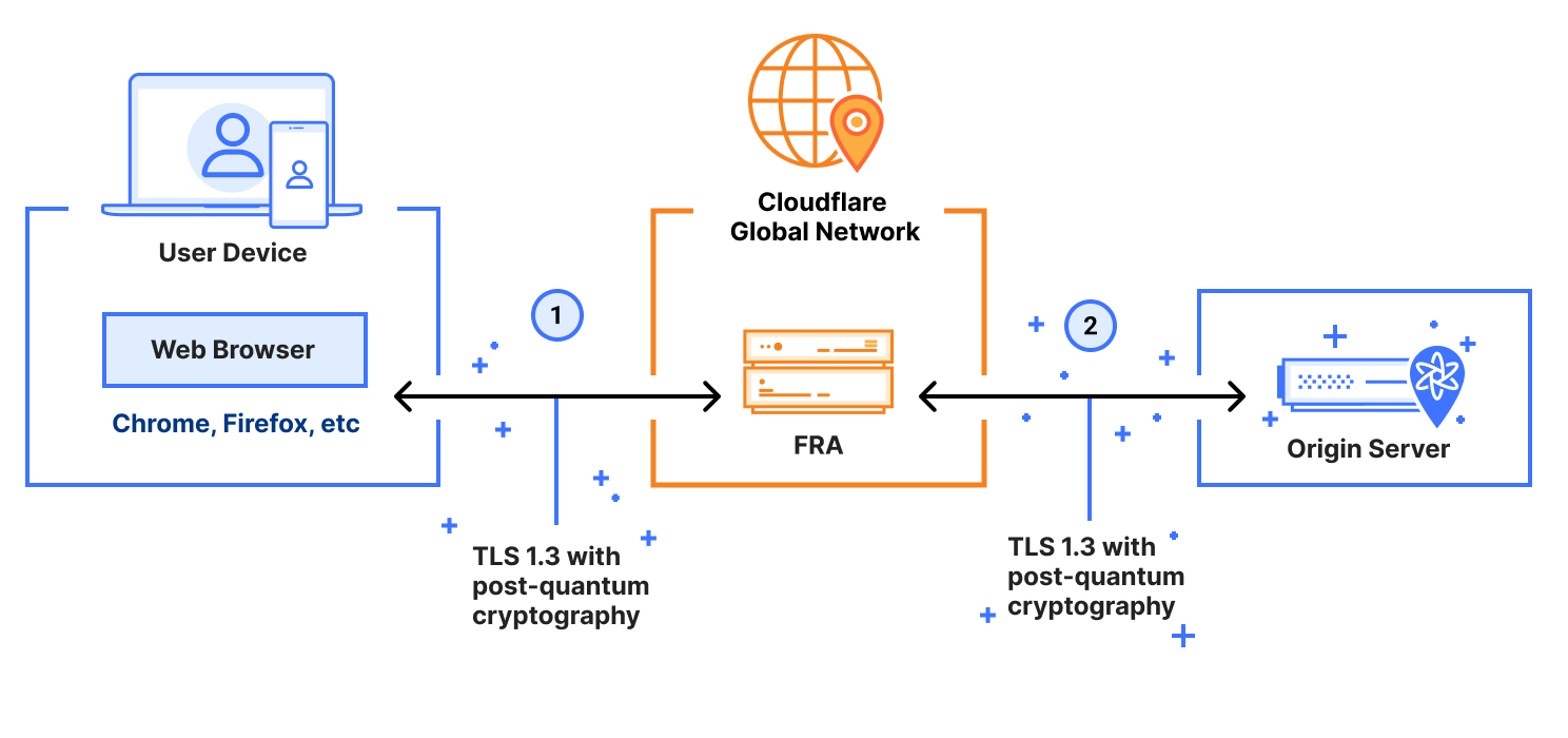
Finally, we note that traffic that on-ramps to Cloudflare One and then egresses to the public Internet can also be protected by our post-quantum Cloudflare Gateway, our Secure Web Gateway (SWG). Here’s a diagram showing how the SWG works:
As discussed in an earlier blog post, our SWG can already support hybrid ML-KEM on traffic from SWG to the origin server (as long as the origin supports hybrid ML-KEM), and on traffic from the client to the SWG (if the client supports hybrid ML-KEM, which is the case for most modern browsers). Importantly, any traffic that onramps to the SWG via a device that has Cloudflare One Client installed is still protected with hybrid ML-KEM — even if the web browser itself does not yet support post-quantum cryptography. This is due to the post-quantum MASQUE tunnel that the Cloudflare One Client establishes to Cloudflare’s global network. The same is true of traffic that onramps to the SWG via a post-quantum Cloudflare IPsec tunnel.
Putting it all together, Cloudflare One now offers post-quantum encryption on our TLS, MASQUE and IPsec on-ramp and off-ramps, and for private network traffic, and to traffic that egresses to the public Internet via our SWG.
The future is quantum-safe
By completing the post-quantum SASE equation with Cloudflare IPsec and the Cloudflare One Appliance, we have extended post-quantum encryption across all our major on-ramps and off-ramps. We have intentionally chosen the path of interoperability and simplicity — the hybrid ML-KEM approach that the IETF and NIST have championed, rather than locking our customers into proprietary implementations, “ciphersuite bloat,” or unnecessary hardware upgrades.
This is the promise of Cloudflare One: a SASE platform that is not only faster and more reliable than the legacy architectures it replaces, but one that provides post-quantum encryption. Whether you are securing a remote worker’s browser or a multi-gigabit data center link, you can now do so with the confidence that your data is protected from harvest-now-decrypt-later attacks and other future-looking threats.
You can sign up here to get a full demo of our post-quantum capabilities across the Cloudflare One SASE platform. We are proud to lead the industry into this new era of cryptography, and we invite you to join us in building a scalable, standards-compliant, and post-quantum Internet.
The Business of Secrets: Adventures in Selling Encryption Around the World by Fred Kinch (May 24, 2024)
From the vantage point of today, it’s surreal reading about the commercial cryptography business in the 1970s. Nobody knew anything. The manufacturers didn’t know whether the cryptography they sold was any good. The customers didn’t know whether the crypto they bought was any good. Everyone pretended to know, thought they knew, or knew better than to even try to know.
The Business of Secrets is the self-published memoirs of Fred Kinch. He was founder and vice president of—mostly sales—at a US cryptographic hardware company called Datotek, from company’s founding in 1969 until 1982. It’s mostly a disjointed collection of stories about the difficulties of selling to governments worldwide, along with descriptions of the highs and (mostly) lows of foreign airlines, foreign hotels, and foreign travel in general. But it’s also about encryption.
Datotek sold cryptographic equipment in the era after rotor machines and before modern academic cryptography. The company initially marketed computer-file encryption, but pivoted to link encryption—low-speed data, voice, fax—because that’s what the market wanted.
These were the years where the NSA hired anyone promising in the field, and routinely classified—and thereby blocked—publication of academic mathematics papers of those they didn’t hire. They controlled the fielding of strong cryptography by aggressively using the International Traffic in Arms regulation. Kinch talks about the difficulties in getting an expert license for Datotek’s products; he didn’t know that the only reason he ever got that license was because the NSA was able to break his company’s stuff. He had no idea that his largest competitor, the Swiss company Crypto AG, was owned and controlled by the CIA and its West German equivalent. “Wouldn’t that have made our life easier if we had known that back in the 1970s?” Yes, it would. But no one knew.
Glimmers of the clandestine world peek out of the book. Countries like France ask detailed tech questions, borrow or buy a couple of units for “evaluation,” and then disappear again. Did they break the encryption? Did they just want to see what their adversaries were using? No one at Datotek knew.
Kinch “carried the key generator logic diagrams and schematics” with him—even today, it’s good practice not to rely on their secrecy for security—but the details seem laughably insecure: four linear shift registers of 29, 23, 13, and 7 bits, variable stepping, and a small nonlinear final transformation. The NSA probably used this as a challenge to its new hires. But Datotek didn’t know that, at the time.
Kinch writes: “The strength of the cryptography had to be accepted on trust and only on trust.” Yes, but it’s so, so weird to read about it in practice. Kinch demonstrated the security of his telephone encryptors by hooking a pair of them up and having people listen to the encrypted voice. It’s rather like demonstrating the safety of a food additive by showing that someone doesn’t immediately fall over dead after eating it. (In one absolutely bizarre anecdote, an Argentine sergeant with a “hearing defect” could understand the scrambled analog voice. Datotek fixed its security, but only offered the upgrade to the Argentines, because no one else complained. As I said, no one knew anything.)
In his postscript, he writes that even if the NSA could break Datotek’s products, they were “vastly superior to what [his customers] had used previously.” Given that the previous devices were electromechanical rotor machines, and that his primary competition was a CIA-run operation, he’s probably right. But even today, we know nothing about any other country’s cryptanalytic capabilities during those decades.
A lot of this book has a “you had to be there” vibe. And it’s mostly tone-deaf. There is no real acknowledgment of the human-rights-abusing countries on Datotek’s customer list, and how their products might have assisted those governments. But it’s a fascinating artifact of an era before commercial cryptography went mainstream, before academic cryptography became approved for US classified data, before those of us outside the triple fences of the NSA understood the mathematics of cryptography.
The Internet is in the midst of one of the most complex transitions in its history: the migration to post-quantum (PQ) cryptography. Making a system safe against quantum attackers isn’t just a matter of replacing elliptic curves and RSA with PQ alternatives, such as ML-KEM and ML-DSA. These algorithms have higher costs than their classical counterparts, making them unsuitable as drop-in replacements in many situations.
Nevertheless, we’re making steady progress on the most important systems. As of this writing, about 50% of TLS connections to Cloudflare’s edge are safe against store-now/harvest-later attacks. Quantum safe authentication is further out, as it will require more significant changes to how certificates work. Nevertheless, this year we’ve taken a major step towards making TLS deployable at scale with PQ certificates.
That said, TLS is only the lowest hanging fruit. There are many more ways we have come to rely on cryptography than key exchange and authentication and which aren’t as easy to migrate. In this blog post, we’ll take a look at Anonymous Credentials (ACs).
ACs solve a common privacy dilemma: how to prove a specific fact (for example that one has had a valid driver’s license for more than three years) without over-sharing personal information (like the place of birth)? Such problems are fundamental to a number of use cases, and ACs may provide the foundation we need to make these applications as private as possible.
Just like for TLS, the central question for ACs is whether there are drop-in, PQ replacements for its classical primitives that will work at the scale required, or will it be necessary to re-engineer the application to mitigate the cost of PQ.
We’ll take a stab at answering this question in this post. We’ll focus primarily on an emerging use case for ACs described in a concurrent post: rate-limiting requests from agentic AI platforms and users. This demanding, high-scale use case is the perfect lens through which to evaluate the practical readiness of today’s post-quantum research. We’ll use it as our guiding problem to measure each cryptographic approach.
We’ll first explore the current landscape of classical AC adoption across the tech industry and the public sector. Then, we’ll discuss what cryptographic researchers are currently looking into on the post-quantum side. Finally, we’ll take a look at what it’ll take to bridge the gap between theory and real-world applications.
While anonymous credentials are only seeing their first real-world deployments in recent years, it is critical to start thinking about the post-quantum challenge concurrently. This isn’t a theoretical, too-soon problem given the store-now decrypt-later threat. If we wait for mass adoption before solving post-quantum anonymous credentials, ACs risk being dead on arrival. Fortunately, our survey of the state of the art shows the field is close to a practical solution. Let’s start by reviewing real-world use-cases of ACs.
Real world (classical) anonymous credentials
In 2026, the European Union is set to launch its digital identity wallet, a system that will allow EU citizens, residents and businesses to digitally attest to their personal attributes. This will enable them, for example, to display their driver’s license on their phone or perform ageverification. Cloudflare’s use cases for ACs are a bit different and revolve around keeping our customers secure by, for example, rate limiting bots and humans as we currently do with Privacy Pass. The EU wallet is a massive undertaking in identity provisioning, and our work operates at a massive scale of traffic processing. Both initiatives are working to solve a shared fundamental problem: allowing an entity to prove a specific attribute about themselves without compromising their privacy by revealing more than they have to.
The EU’s goal is a fully mobile, secure, and user-friendly digital ID. The current technical plan is ambitious, as laid out in the Architecture Reference Framework (ARF). It defines the key privacy goals of unlinkability to guarantee that if a user presents attributes multiple times, the recipients cannot link these separate presentations to conclude that they concern the same user. However, currently proposed solutions fail to achieve this. The framework correctly identifies the core problem: attestations contain unique, fixed elements such as hash values, […], public keys, and signatures that colluding entities could store and compare to track individuals.
In its present form, the ARF’s recommendation to mitigate cross-session linkability is limited-time attestations. The framework acknowledges in the text that this would only partially mitigate Relying Party linkability. An alternative proposal that would mitigate linkability risks are single-use credentials. They are not considered at the moment due to complexity and management overhead. The framework therefore leans on organisational and enforcement measures to deter collusion instead of providing a stronger guarantee backed by cryptography.
This reliance on trust assumptions could become problematic, especially in the sensitive context of digital identity. When asked for feedback, cryptographic researchers agree that the proper solution would be to adopt anonymous credentials. However, this solution presents a long-term challenge. Well-studied methods for anonymous credentials, such as those based on BBS signatures, are vulnerable to quantum computers. While some anonymousschemes are PQ-unlinkable, meaning that user privacy is preserved even when cryptographically relevant quantum computers exist, new credentials could be forged. This may be an attractive target for, say, a nation state actor.
New cryptography also faces deployment challenges: in the EU, only approved cryptographic primitives, as listed in the SOG-IS catalogue, can be used. At the time of writing, this catalogue is limited to established algorithms such as RSA or ECDSA. But when it comes to post-quantum cryptography, SOG-IS is leaving the problem wide open.
The wallet’s first deployment will not be quantum-secure. However, with the transition to post-quantum algorithms being ahead of us, as soon as 2030 for high-risk use cases per the EU roadmap, research in a post-quantum compatible alternative for anonymous credentials is critical. This will encompassstandardizing more cryptography.
Finally, ongoing efforts at the Internet Engineering Task Force (IETF)aimto build a more private Internet by standardizing advanced cryptographic techniques. Active individual drafts (i.e., not yet adopted by a working group), such as Longfellow and Anonymous Credit Tokens (ACT), and adopted drafts like Anonymous Rate-limited Credentials (ARC), propose more flexible multi-show anonymous credentials that incorporate developments over the last several years. At IETF 117 in 2023, post-quantum anonymous credentials and deployable generic anonymous credentials were presented as a research opportunity. Check out our post on rate limiting agents for details.
Before we get into the state-of-the-art for PQ, allow us to try to crystalize a set of requirements for real world applications.
Requirements
Given the diversity of use cases, adoption of ACs will be made easier by the fact that they can be built from a handful of powerful primitives. (More on this in our concurrent post.) As we’ll see in the next section, we don’t yet have drop-in, PQ alternatives for these kinds of primitives. The “building blocks” of PQ ACs are likely to look quite different, and we’re going to know something about what we’re building towards.
For our purposes, we can think of an anonymous credential as a kind of fancy blind signature. What’s that you ask? A blind signature scheme has two phases: issuance, in which the server signs a message chosen by the client; and presentation, in which the client reveals the message and the signature to the server. The scheme should be unlinkable in the sense that the server can’t link any message and signature to the run of the issuance protocol in which it was produced. It should also be unforgeable in the sense that no client can produce a valid signature without interacting with the server.
The key difference between ACs and blind signatures is that, during presentation of an AC, the client only presents part of the message in plaintext; the rest of the message is kept secret. Typically, the message has three components:
Private state, such as a counter that, for example, keeps track of the number of times the credential was presented. The client would prove to the server that the state is “valid”, for example, a counter with value $0 \leq C \leq N$, without revealing $C$. In many situations, it’s desirable to allow the server to update this state upon successful presentation, for example, by decrementing the counter. In the context of rate limiting, this is the number of how many requests are left for a credential.
A random value called the nullifier that is revealed to the server during presentation. In rate-limiting, the nullifier prevents a user from spending a credential with a given state more than once.
Public attributes known to both the client and server that bind the AC to some application context. For example, this might represent the window of time in which the credential is valid (without revealing the exact time it was issued).
Such ACs are well-suited for rate limiting requests made by the client. Here the idea is to prevent the client from making more than some maximum number of requests during the credential’s lifetime. For example, if the presentation limit is 1,000 and the validity window is one hour, then the clients can make up to 0.27 requests/second on average before it gets throttled.
It’s usually desirable to enforce rate limits on a per-origin basis. This means that if the presentation limit is 1,000, then the client can make at most 1,000 requests to any website that can verify the credential. Moreover, it can do so safely, i.e., without breaking unlinkability across these sites.
The current generation of ACs being considered for standardization at IETF are only privately verifiable, meaning the server issuing the credential (the issuer) must share a private key with the server verifying the credential (the origin). This will be sufficient for some deployment scenarios, but many will require public verifiability, where the origin only needs the issuer’s public key. This is possible with BBS-based credentials, for example.
Finally, let us say a few words about round complexity. An AC is round optimal if issuance and presentation both complete in a single HTTP request and response. In our survey of PQ ACs, we found a number of papers that discovered neat tricks that reduce bandwidth (the total number of bits transferred between the client and server) at the cost of additional rounds. However, for use cases like ours, round optimality is an absolute necessity, especially for presentation. Not only do multiple rounds have a high impact on latency, they also make the implementation far more complex.
Within these constraints, our goal is to develop PQ ACs that have as low communication cost (i.e., bandwidth consumption) and runtime as possible in the context of rate-limiting.
“Ideal world” (PQ) anonymous credentials
The academic community has produced a number of promising post-quantum ACs. In our survey of the state of the art, we evaluated several leading schemes, scoring them on their underlying primitives and performance to determine which are truly ready for the Internet. To understand the challenges, it is essential to first grasp the cryptographic building blocks used in ACs today. We’ll now discuss some of the core concepts that frequently appear in the field.
Relevant cryptographic paradigms
Zero-knowledge proofs
Zero-knowledge proofs (ZKPs) are a cryptographic protocol that allows a prover to convince a verifier that a statement is true without revealing the secret information, or witness. ZKPs play a central role in ACs: they allow proving statements of the secret part of the credential’s state without revealing the state itself. This is achieved by transforming the statement into a mathematical representation, such as a set of polynomial equations over a finite field. The prover then generates a proof by performing complex operations on this representation, which can only be completed correctly if they possess the valid witness.
General-purpose ZKP systems, like Scalable Transparent Arguments of Knowledge (STARKs), can prove the integrity of any computation up to a certain size. In a STARK-based system, the computational trace is represented as a set of polynomials. The prover then constructs a proof by evaluating these polynomials and committing to them using cryptographic hash functions. The verifier can then perform a quick probabilistic check on this proof to confirm that the original computation was executed correctly. Since the proof itself is just a collection of hashes and sampled polynomial values, it is secure against quantum computers, providing a statistically sound guarantee that the claimed result is valid.
Cut-and-Choose
Cut-and-choose is a cryptographic technique designed to ensure a prover’s honest behaviour by having a verifier check a random subset of their work. The prover first commits to multiple instances of a computation, after which the verifier randomly chooses a portion to be cut open by revealing the underlying secrets for inspection. If this revealed subset is correct, the verifier gains high statistical confidence that the remaining, un-opened instances are also correct.
This technique is important because while it is a generic tool used to build protocols secure against malicious adversaries, it also serves as a crucial case study. Its security is not trivial; for example, practical attacks on cut-and-choose schemes built with (post-quantum) homomorphic encryption have succeeded by attacking the algebraic structure of the encoding, not the encryption itself. This highlights that even generic constructions must be carefully analyzed in their specific implementation to prevent subtle vulnerabilities and information leaks.
Sigma Protocols
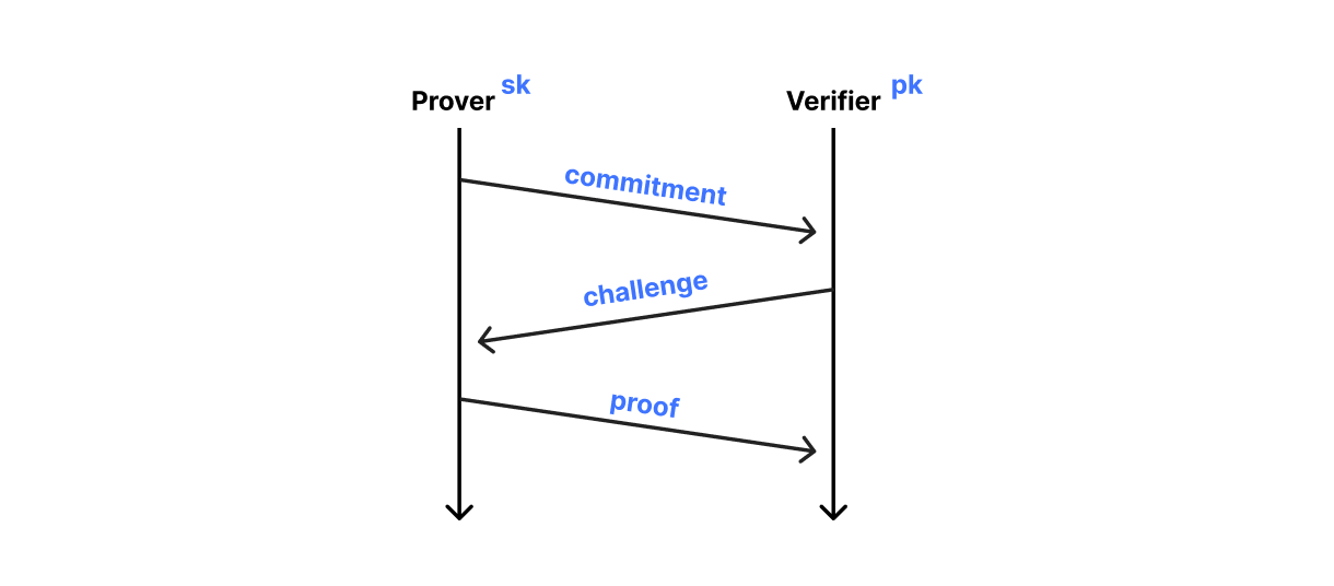
Sigma protocols follow a more structured approach that does not require us to throw away any computations. The three-move protocol starts with a commitment phase where the prover generates some randomness, which is added to the input to generate the commitment, and sends the commitment to the verifier. Then, the verifier challenges the prover with an unpredictable challenge. To finish the proof, the prover provides a response in which they combine the initial randomness with the verifier’s challenge in a way that is only possible if the secret value, such as the solution to a discrete logarithm problem, is known.
Depiction of a Sigma protocol flow, where the prover commits to their witness $w$, the verifier challenges the prover to prove knowledge about $w$, and the prover responds with a mathematical statement that the verifier can either accept or reject.
In practice, the prover and verifier don’t run this interactive protocol. Instead, they make it non-interactive using a technique known as the Fiat-Shamir transformation. The idea is that the prover generates the challenge itself, by deriving it from its own commitment. It may sound a bit odd, but it works quite well. In fact, it’s the basis of signatures like ECDSA and even PQ signatures like ML-DSA.
MPC in the head
Multi-party computation (MPC) is a cryptographic tool that allows multiple parties to jointly compute a function over their inputs without revealing their individual inputs to the other parties. MPC in the Head (MPCitH) is a technique to generate zero-knowledge proofs by simulating a multi-party protocol in the head of the prover.
The prover simulates the state and communication for each virtual party, commits to these simulations, and shows the commitments to the verifier. The verifier then challenges the prover to open a subset of these virtual parties. Since MPC protocols are secure even if a minority of parties are dishonest, revealing this subset doesn’t leak the secret, yet it convinces the verifier that the overall computation was correct.
This paradigm is particularly useful to us because it’s a flexible way to build post-quantum secure ZKPs. MPCitH constructions build their security from symmetric-key primitives (like hash functions). This approach is also transparent, requiring no trusted setup. While STARKs share these post-quantum and transparent properties, MPCitH often offers faster prover times for many computations. Its primary trade-off, however, is that its proofs scale linearly with the size of the circuit to prove, while STARKs are succinct, meaning their proof size grows much slower.
Rejection sampling
When a randomness source is biased or outputs numbers outside the desired range, rejection sampling can correct the distribution. For example, imagine you need a random number between 1 and 10, but your computer only gives you random numbers between 0 and 255. (Indeed, this is the case!) The rejection sampling algorithm calls the RNG until it outputs a number below 11 and above 0:
Calling the generator over and over again may seem a bit wasteful. An efficient implementation can be realized with an eXtendable Output Function (XOF). A XOF takes an input, for example a seed, and computes an arbitrarily-long output. An example is the SHAKE family (part of the SHA3 standard), and the recently proposed round-reduced version of SHAKE called TurboSHAKE.
Let’s imagine you want to have three numbers between 1 and 10. Instead of calling the XOF over and over, you can also ask the XOF for several bytes of output. Since each byte has a probability of 3.52% to be in range, asking the XOF for 174 bytes is enough to have a greater than 99% chance of finding at least three usable numbers. In fact, we can be even smarter than this: 10 fits in four bits, so we can split the output bytes into lower and higher nibbles. The probability of a nibble being in the desired range is now 56.4%:
Rejection sampling by batching queries.
Rejection sampling is a part of many cryptographic primitives, including many we’ll discuss in the schemes we look at below.
Building post-quantum ACs
Classical anonymous credentials (ACs), such as ARC and ACT, are built from algebraic groups- specifically, elliptic curves, which are very efficient. Their security relies on the assumption that certain mathematical problems over these groups are computationally hard. The premise of post-quantum cryptography, however, is that quantum computers can solve these supposedly hard problems. The most intuitive solution is to replace elliptic curves with a post-quantum alternative. In fact, cryptographers have been working on a replacement for a number of years: CSIDH.
This raises the key question: can we simply adapt a scheme like ARC by replacing its elliptic curves with CSIDH? The short answer is no, due to a critical roadblock in constructing the necessary zero-knowledge proofs. While we can, in theory, build the required Sigma protocols or MPC-in-the-Head (MPCitH) proofs from CSIDH, they have a prerequisite that makes them unusable in practice: they require a trusted setup to ensure the prover cannot cheat. This requirement is a non-starter, as no algorithm for performing a trusted setup in CSIDH exists. The trusted setup for sigma protocols can be replaced by a combination of generic techniques from multi-party computation and cut-and-choose protocols, but that adds significant computation cost to the already computationally expensive isogeny operations.
This specific difficulty highlights a more general principle. The high efficiency of classical credentials like ARC is deeply tied to the rich algebraic structure of elliptic curves. Swapping this component for a post-quantum alternative, or moving to generic constructions, fundamentally alters the design and its trade-offs. We must therefore accept that post-quantum anonymous credentials cannot be a simple “lift-and-shift” of today’s schemes. They will require new designs built from different cryptographic primitives, such as lattices or hash functions.
Prefabricated schemes from generic approaches
At Cloudflare, we explored a post-quantum privacy pass construction in 2023 that closely resembles the functionality needed for anonymous credentials. The main result is a generic construction that composes separate, quantum-secure building blocks: a digital signature scheme and a general-purpose ZKP system:
The figure shows a cryptographic protocol divided into two main phases: (1.) Issuance: The user commits to a message (without revealing it) and sends the commitment to the server. The server signs the commitment and returns this signed commitment, which serves as a token. The user verifies the server’s signature. (2.) Redemption: To use the token, the user presents it and constructs a proof. This proof demonstrates they have a valid signature on the commitment and opens the commitment to reveal the original message. If the server validates the proof, the user and server continue (e.g., to access a rate-limited origin).
The main appeal of this modular design is its flexibility. The experimental implementation uses a modified version of the signature ML-DSA signatures and STARKs, but the components can be easily swapped out. The design provides strong, composable security guarantees derived directly from the underlying parts. A significant speedup for the construction came from replacing the hash function SHA3 in ML-DSA with the zero-knowledge friendly Poseidon.
However, the modularity of our post-quantum Privacy Pass construction incurs a significant performance overhead demonstrated in a clear trade-off between proof generation time and size: a fast 300 ms proof generation requires a large 173 kB signature, while a 4.8s proof generation time cuts the size of the signature nearly in half. A balanced parameter set, which serves as a good benchmark for any dedicated solution to beat, took 660 ms to sign and resulted in a 112 kB signature. The implementation is currently a proof of concept, with perhaps some room for optimization. Alternatively, a different signature like FN-DSA could offer speed improvements: while its issuance is more complex, its verification is far more straightforward, boiling down to a simple hash-to-lattice computation and a norm check.
However, while this construction gives a functional baseline, these figures highlight the performance limitations for a real-time rate limiting system, where every millisecond counts. The 660 ms signing time strongly motivates the development of dedicated cryptographic constructions that trade some of the modularity for performance.
Solid structure: Lattices
Lattices are a natural starting point when discussing potential post-quantum AC candidates. NIST standardized ML-DSA and ML-KEM as signature and KEM algorithms, both of which are based on lattices. So, are lattices the answer to post-quantum anonymous credentials?
The answer is a bit nuanced. While explicit anonymous credential schemes from lattices exist, they have shortcomings that prevent real-world deployment: for example, a recent scheme sacrifices round-optimality for smaller communication size, which is unacceptable for a service like Privacy Pass where every second counts. Given that our RTT is 100ms or less for the majority of users, each extra communication round adds tangible latency especially for those on slower Internet connections. When the final credential size is still over 100 kB, the trade-offs are hard to justify. So, our search continues. We expand our horizon by looking into blind signatures and whether we can adapt them for anonymous credentials.
Two-step approach: Hash-and-sign
A prominent paradigm in lattice-based signatures is the hash-and-sign construction. Here, the message is first hashed to a point in the lattice. Then, the signer uses their secret key, a lattice trapdoor, to generate a vector that, when multiplied with the private key, evaluates to the hashed point in the lattice. This is the core mechanism behind signature schemes like FN-DSA.
Adapting hash-and-sign for blind signatures is tricky, since the signer may not learn the message. This introduces a significant security challenge: If the user can request signatures on arbitrary points, they can mount an attack to extract the trapdoor by repeatedly requesting signatures for carefully chosen arbitrary points. These points can be used to reconstruct a short basis, which is equivalent to a key recovery.
The standard defense against this attack is to require the user to prove in zero-knowledge that the point they are asking to be signed is the blinded output of the specified hash function. However, proving hash preimages leads to the same problem as in the generic post-quantum privacy pass paper: proving a conventional hash function (like SHA3) inside a ZKP is computationally expensive and has a large communication complexity.
This difficult trade-off is at the heart of recent academic work. The state-of-the-art paper presents two lattice-based blind signature schemes with small signature sizes of 22 KB for a signature and 48 kB for a privately-verifiable protocol that may be more useful in a setting like anonymous credential. However, this focus on the final signature size comes at the cost of an impractical issuance. The user must provide ZKPs for the correct hash and lattice relations that, by the paper’s own analysis, can add to several hundred kilobytes and take 20 seconds to generate and 10 seconds to verify.
While these results are valuable for advancing the field, this trade-off is a significant barrier for any large-scale, practical system. For our use case, a protocol that increases the final signature size moderately in exchange for a more efficient and lightweight issuance process would be a more suitable and promising direction.
Best of two signatures: Hash-and-sign with aborts
A promising technique for blind signatures combines the hash-and-sign paradigm with Fiat-Shamir with aborts, a method that relies on rejection sampling signatures. In this approach, the signer repeatedly attempts to generate a signature and aborts any result that may leak information about the secret key. This process ensures the final signature is statistically independent of the key and is used in modern signatures like ML-DSA. The Phoenix signature scheme uses hash-and-sign with aborts, where a message is first hashed into the lattice and signed, with rejection sampling employed to break the dependency between the signature and the private key.
Building on this foundation is an anonymous credential scheme for hash-and-sign with aborts. The main improvement over hash-and-sign anonymous credentials is that, instead of proving the validity of a hash, the user commits to their attributes, which avoids costly zero-knowledge proofs.
The scheme is fully implemented and credentials with attribute proofs just under 80 KB and signatures under 7 kB. The scheme takes less than 400 ms for issuance and 500 ms for showing the credential. The protocol also has a lot of features necessary for anonymous credentials, allowing users to prove relations between attributes and request pseudonyms for different instances.
This research presents a compelling step towards real-world deployability by combining state-of-the-art techniques to achieve a much healthier balance between performance and security. While the underlying mathematics are a bit more complex, the scheme is fully implemented and with a proof of knowledge of a signature at 40 kB and a prover time under a second, the scheme stands out as a great contender. However, for practical deployment, these figures would likely need a significant speedup to be usable in real-time systems. An improvement seems plausible, given recent advances in lattice samplers. Though the exact scale we can achieve is unclear. Still, we think it would be worthwhile to nudge the underlying design paradigm a little closer to our use cases.
Do it yourself: MPC-in-the-head
While the lattice-based hash-and-sign with aborts scheme provides one path to post-quantum signatures, an alternative approach is emerging from the MPCitH variant VOLE-in-the-Head (VOLEitH).
This scheme builds on Vector Oblivious Linear Evaluation (VOLE), an interactive protocol where one party’s input vector is processed with another’s secret value delta, creating a correlation. This VOLE correlation is used as a cryptographic commitment to the prover’s input. The system provides a zero-knowledge proof because the prover is bound by this correlation and cannot forge a solution without knowing the secret delta. The verifier, in turn, just has to verify that the final equation holds when the commitment is opened. This system is linearly homomorphic, which means that two commitments can be combined. This property is ideal for the commit-and-prove paradigm, where the prover first commits to the witnesses and then proves the validity of the circuit gate by gate. The primary trade-off is that the proofs are linear in the size of the circuit, but they offer substantially better runtimes. We also use linear-sized proofs for ARC and ACT.
Example of evaluating a circuit gate by first committing to each wire and then proving the composition. This is easy for linear gates.
This commit-and-prove approach allows VOLEitH to efficiently prove the evaluation of symmetric ciphers, which are quantum-resistant. The transformation to a non-interactive protocol follows the standard MPCitH method: the prover commits to all secret values, a challenge is used to select a subset to reveal, and the prover proves consistency.
Efficient implementations operate over two mathematical fields (binary and prime) simultaneously, allowing these ZK circuits to handle both arithmetic and bitwise functions (like XORs) efficiently. Based on this foundation, a recent talk teased the potential for blind signatures from the multivariate quadratic signature scheme MAYO with sizes of just 7.5 kB and signing/verification times under 50 ms.
The VOLEitH approach, as a general-purpose solution system, represents a promising new direction for performant constructions. There are a numberofcompetingin-the-head schemes in the NIST competition for additional signature schemes, including one based on VOLEitH. The current VOLEitH literature focuses on high-performance digital signatures, and an explicit construction for a full anonymous credential system has not yet been proposed. This means that features standard to ACs, such as multi-show unlinkability or the ability to prove relations between attributes, are not yet part of the design, whereas they are explicitly supported by the lattice construction. However, the preliminary results show great potential for performance, and it will be interesting to see the continued cryptanalysis and feature development from this line of VOLEitH in the area of anonymous credentials, especially since the general-purpose construction allows adding features easily.
Medium: promising research direction, no full solution available so far
Closing the gap
My (that is Lena’s) internship focused on a critical question: what should we look at next to build ACs for the Internet? For us, “the right direction” means developing protocols that can be integrated with real world applications, and developed collaboratively at the IETF. To make these a reality, we need researchers to look beyond blind signatures; we need a complete privacy-preserving protocol that combines blind signatures with efficient zero-knowledge proofs and properties like multi-show credentials that have an internal state. The issuance should also be sublinear in communication size with the number of presentations.
So, with the transition to post-quantum cryptography on the horizon, what are our thoughts on the current IETF proposals? A 2022 NIST presentation on the current state of anonymous credentials states that efficient post-quantum secure solutions are basically non-existent. We argue that the last three years show nice developments in lattices and MPCitH anonymous credentials, but efficient post-quantum protocols still need work. Moving protocols into a post-quantum world isn’t just a matter of swapping out old algorithms for new ones. A common approach on constructing post-quantum versions of classical protocols is swapping out the building blocks for their quantum-secure counterpart.
We believe this approach is essential, but not forward-looking. In addition to identifying how modern concerns can be accommodated on old cryptographic designs, we should be building new, post-quantum native protocols.
For ARC, the conceptual path to a post-quantum construction seems relatively straightforward. The underlying cryptography follows a similar structure as the lattice-based anonymous credentials, or, when accepting a protocol with fewer features, the generic post-quantum privacy-pass construction. However, we need to support per-origin rate-limiting, which allows us to transform a token at an origin without leaking us being able to link the redemption to redemptions at other origins, a feature that none of the post-quantum anonymous credential protocols or blind signatures support. Also, ARC is sublinear in communication size with respect to the number of tokens issued, which so far only the hash-and-sign with abort lattices achieve, although the notion of “limited shows” is not present in the current proposal. In addition, it would be great to gauge efficient implementations, especially for blind signatures, as well as looking into efficient zero-knowledge proofs.
For ACT, we need the protocols for ARC and an additional state. Even for the simplest counter, we need the ability to homomorphically subtract from that balance within the credential itself. This is a much more complex cryptographic requirement. It would also be interesting to see a post-quantum double-spend prevention that enforces the sequential nature of ACT.
Working on ACs and other privacy-preserving cryptography inevitably leads to a major bottleneck: efficient zero-knowledge proofs, or to be more exact, efficiently proving hash function evaluations. In a ZK circuit, multiplications are expensive. Each wire in the circuit that performs a multiplication requires a cryptographic commitment, which adds communication overhead. In contrast, other operations like XOR can be virtually “free.” This makes a huge difference in performance. For example, SHAKE (the primitive used in ML-DSA) can be orders of magnitude slower than arithmetization-friendly hash functions inside a ZKP. This is why researchers and implementers are already using Poseidon or Poseidon2 to make their protocols faster.
Currently, Ethereum is seriously considering migrating Ethereum to the Poseidon hash and calls for cryptanalysis, but there is no indication of standardization. This is a problem: papers increasingly use different instantiations of Poseidon to fit their use-case, and there aremoreandmorezero–knowledgefriendlyhashfunctionscomingout, tailored to different use-cases. We would like to see at least one XOF and one hash each for a prime field and for a binary field, ideally with some security levels. And also, is Poseidon the best or just the most well-known ZK friendly cipher? Is it always secure against quantum computers (like we believe AES to be), and are there other attacks like the recentattacks on round-reduced versions?
Looking at algebra and zero-knowledge brings us to a fundamental debate in modern cryptography. Imagine a line representing the spectrum of research: On one end, you have protocols built on very well-analyzed standard assumptions like the SIS problem on lattices or the collision resistance of SHA3. On the other end, you have protocols that gain massive efficiency by using more algebraic structure, which in turn relies on newer, stronger cryptographic assumptions. Breaking novel hash functions is somewhere in the middle.
The answer for the Internet can’t just be to relent and stay at the left end of our graph to be safe. For the ecosystem to move forward, we need to have confidence in both. We need more research to validate the security of ZK-friendly primitives like Poseidon, and we need more scrutiny on the stronger assumptions that enable efficient algebraic methods.
Conclusion
As we’ve explored, the cryptographic properties that make classical ACs efficient, particularly the rich structure of elliptic curves, do not have direct post-quantum equivalents. Our survey of the state of the art from generic compositions using STARKs, to various lattice-based schemes, and promising new directions like MPC-in-the-head, reveals a field full of potential but with no clear winner. The trade-offs between communication cost, computational cost, and protocol rounds remain a significant barrier to practical, large-scale deployment, especially in comparison to elliptic curve constructions.
To bridge this gap, we must move beyond simply building post-quantum blind signatures. We challenge our colleagues in academia and industry to develop complete, post-quantum native protocols that address real-world needs. This includes supporting essential features like the per-origin rate-limiting required for ARC or the complex stateful credentials needed for ACT.
A critical bottleneck for all these approaches is the lack of efficient, standardized, and well-analyzed zero-knowledge-friendly hash functions. We need to research zero-knowledge friendly primitives and build industry-wide confidence to enable efficient post-quantum privacy.
If you’re working on these problems, or you have experience in the management and deployment of classical credentials, now is the time to engage. The world is rapidly adopting credentials for everything from digital identity to bot management, and it is our collective responsibility to ensure these systems are private and secure for a post-quantum future. We can tell for certain that there are more discussions to be had, and if you’re interested in helping to build this more secure and private digital world, we’re hiring 1,111 interns over the course of next year, and have open positions!
Ultimately, the architects settled on a creative solution. Rather than bolt KEM onto the existing double ratchet, they allowed it to remain more or less the same as it had been. Then they used the new quantum-safe ratchet to implement a parallel secure messaging system.
Now, when the protocol encrypts a message, it sources encryption keys from both the classic Double Ratchet and the new ratchet. It then mixes the two keys together (using a cryptographic key derivation function) to get a new encryption key that has all of the security of the classical Double Ratchet but now has quantum security, too.
The Signal engineers have given this third ratchet the formal name: Sparse Post Quantum Ratchet, or SPQR for short. The third ratchet was designed in collaboration with PQShield, AIST, and New York University. The developers presented the erasure-code-based chunking and the high-level Triple Ratchet design at the Eurocrypt 2025 conference. At the Usenix 25 conference, they discussed the six options they considered for adding quantum-safe forward secrecy and post-compromise security and why SPQR and one other stood out. Presentations at the NIST PQC Standardization Conference and the Cryptographic Applications Workshop explain the details of chunking, the design challenges, and how the protocol had to be adapted to use the standardized ML-KEM.
Jacomme further observed:
The final thing interesting for the triple ratchet is that it nicely combines the best of both worlds. Between two users, you have a classical DH-based ratchet going on one side, and fully independently, a KEM-based ratchet is going on. Then, whenever you need to encrypt something, you get a key from both, and mix it up to get the actual encryption key. So, even if one ratchet is fully broken, be it because there is now a quantum computer, or because somebody manages to break either elliptic curves or ML-KEM, or because the implementation of one is flawed, or…, the Signal message will still be protected by the second ratchet. In a sense, this update can be seen, of course simplifying, as doubling the security of the ratchet part of Signal, and is a cool thing even for people that don’t care about quantum computers.
The world is in a race to build its first quantum computer capable of solving practical problems not feasible on even the largest conventional supercomputers. While the quantum computing paradigm promises many benefits, it also threatens the security of the Internet by breaking much of the cryptography we have come to rely on.
To mitigate this threat, Cloudflare is helping to migrate the Internet to Post-Quantum (PQ) cryptography. Today, about 50% of traffic to Cloudflare’s edge network is protected against the most urgent threat: an attacker who can intercept and store encrypted traffic today and then decrypt it in the future with the help of a quantum computer. This is referred to as the harvest now, decrypt laterthreat.
However, this is just one of the threats we need to address. A quantum computer can also be used to crack a server’s TLS certificate, allowing an attacker to impersonate the server to unsuspecting clients. The good news is that we already have PQ algorithms we can use for quantum-safe authentication. The bad news is that adoption of these algorithms in TLS will require significant changes to one of the most complex and security-critical systems on the Internet: the Web Public-Key Infrastructure (WebPKI).
The central problem is the sheer size of these new algorithms: signatures for ML-DSA-44, one of the most performant PQ algorithms standardized by NIST, are 2,420 bytes long, compared to just 64 bytes for ECDSA-P256, the most popular non-PQ signature in use today; and its public keys are 1,312 bytes long, compared to just 64 bytes for ECDSA. That’s a roughly 20-fold increase in size. Worse yet, the average TLS handshake includes a number of public keys and signatures, adding up to 10s of kilobytes of overhead per handshake. This is enough to have a noticeable impact on the performance of TLS.
That makes drop-in PQ certificates a tough sell to enable today: they don’t bring any security benefit before Q-day — the day a cryptographically relevant quantum computer arrives — but they do degrade performance. We could sit and wait until Q-day is a year away, but that’s playing with fire. Migrations always take longer than expected, and by waiting we risk the security and privacy of the Internet, which is dear to us.
It’s clear that we must find a way to make post-quantum certificates cheap enough to deploy today by default for everyone — not just those that can afford it. In this post, we’ll introduce you to the plan we’ve brought together with industry partners to the IETF to redesign the WebPKI in order to allow a smooth transition to PQ authentication with no performance impact (and perhaps a performance improvement!). We’ll provide an overview of one concrete proposal, called Merkle Tree Certificates (MTCs), whose goal is to whittle down the number of public keys and signatures in the TLS handshake to the bare minimum required.
But talk is cheap. We knowfromexperience that, as with any change to the Internet, it’s crucial to test early and often. Today we’re announcing our intent to deploy MTCs on an experimental basis in collaboration with Chrome Security. In this post, we’ll describe the scope of this experiment, what we hope to learn from it, and how we’ll make sure it’s done safely.
The WebPKI today — an old system with many patches
Why does the TLS handshake have so many public keys and signatures?
Let’s start with Cryptography 101. When your browser connects to a website, it asks the server to authenticate itself to make sure it’s talking to the real server and not an impersonator. This is usually achieved with a cryptographic primitive known as a digital signature scheme (e.g., ECDSA or ML-DSA). In TLS, the server signs the messages exchanged between the client and server using its secret key, and the client verifies the signature using the server’s public key. In this way, the server confirms to the client that they’ve had the same conversation, since only the server could have produced a valid signature.
If the client already knows the server’s public key, then only 1 signature is required to authenticate the server. In practice, however, this is not really an option. The web today is made up of around a billion TLS servers, so it would be unrealistic to provision every client with the public key of every server. What’s more, the set of public keys will change over time as new servers come online and existing ones rotate their keys, so we would need some way of pushing these changes to clients.
This scaling problem is at the heart of the design of all PKIs.
Trust is transitive
Instead of expecting the client to know the server’s public key in advance, the server might just send its public key during the TLS handshake. But how does the client know that the public key actually belongs to the server? This is the job of a certificate.
A certificate binds a public key to the identity of the server — usually its DNS name, e.g., cloudflareresearch.com. The certificate is signed by a Certification Authority (CA) whose public key is known to the client. In addition to verifying the server’s handshake signature, the client verifies the signature of this certificate. This establishes a chain of trust: by accepting the certificate, the client is trusting that the CA verified that the public key actually belongs to the server with that identity.
Clients are typically configured to trust many CAs and must be provisioned with a public key for each. Things are much easier however, since there are only 100s of CAs instead of billions. In addition, new certificates can be created without having to update clients.
These efficiencies come at a relatively low cost: for those counting at home, that’s +1 signature and +1 public key, for a total of 2 signatures and 1 public key per TLS handshake.
That’s not the end of the story, however. As the WebPKI has evolved, so have these chains of trust grown a bit longer. These days it’s common for a chain to consist of two or more certificates rather than just one. This is because CAs sometimes need to rotatetheir keys, just as servers do. But before they can start using the new key, they must distribute the corresponding public key to clients. This takes time, since it requires billions of clients to update their trust stores. To bridge the gap, the CA will sometimes use the old key to issue a certificate for the new one and append this certificate to the end of the chain.
That’s +1 signature and +1 public key, which brings us to 3 signatures and 2 public keys. And we still have a little ways to go.
Trust but verify
The main job of a CA is to verify that a server has control over the domain for which it’s requesting a certificate. This process has evolved over the years from a high-touch, CA-specific process to a standardized, mostly automated process used for issuing most certificates on the web. (Not all CAs fully support automation, however.) This evolution is marked by a number of security incidents in which a certificate was mis-issued to a party other than the server, allowing that party to impersonate the server to any client that trusts the CA.
Automation helps, but attacks are still possible, and mistakes are almost inevitable. Earlier this year, several certificates for Cloudflare’s encrypted 1.1.1.1 resolver were issued without our involvement or authorization. This apparently occurred by accident, but it nonetheless put users of 1.1.1.1 at risk. (The mis-issued certificates have since been revoked.)
Ensuring mis-issuance is detectable is the job of the Certificate Transparency (CT) ecosystem. The basic idea is that each certificate issued by a CA gets added to a public log. Servers can audit these logs for certificates issued in their name. If ever a certificate is issued that they didn’t request itself, the server operator can prove the issuance happened, and the PKI ecosystem can take action to prevent the certificate from being trusted by clients.
Major browsers, including Firefox and Chrome and its derivatives, require certificates to be logged before they can be trusted. For example, Chrome, Safari, and Firefox will only accept the server’s certificate if it appears in at least two logs the browser is configured to trust. This policy is easy to state, but tricky to implement in practice:
Operating a CT log has historically been fairly expensive. Logs ingest billions of certificates over their lifetimes: when an incident happens, or even just under high load, it can take some time for a log to make a new entry available for auditors.
Clients can’t really audit logs themselves, since this would expose their browsing history (i.e., the servers they wanted to connect to) to the log operators.
The solution to both problems is to include a signature from the CT log along with the certificate. The signature is produced immediately in response to a request to log a certificate, and attests to the log’s intent to include the certificate in the log within 24 hours.
Per browser policy, certificate transparency adds +2 signatures to the TLS handshake, one for each log. This brings us to a total of 5 signatures and 2 public keys in a typical handshake on the public web.
The future WebPKI
The WebPKI is a living, breathing, and highly distributed system. We’ve had to patch it a number of times over the years to keep it going, but on balance it has served our needs quite well — until now.
Previously, whenever we needed to update something in the WebPKI, we would tack on another signature. This strategy has worked because conventional cryptography is so cheap. But 5 signatures and 2 public keys on average for each TLS handshake is simply too much to cope with for the larger PQ signatures that are coming.
The good news is that by moving what we already have around in clever ways, we can drastically reduce the number of signatures we need.
Crash course on Merkle Tree Certificates
Merkle Tree Certificates (MTCs) is a proposal for the next generation of the WebPKI that we are implementing and plan to deploy on an experimental basis. Its key features are as follows:
All the information a client needs to validate a Merkle Tree Certificate can be disseminated out-of-band. If the client is sufficiently up-to-date, then the TLS handshake needs just 1 signature, 1 public key, and 1 Merkle tree inclusion proof. This is quite small, even if we use post-quantum algorithms.
The MTC specification makes certificate transparency a first class feature of the PKI by having each CA run its own log of exactly the certificates they issue.
Let’s poke our head under the hood a little. Below we have an MTC generated by one of our internal tests. This would be transmitted from the server to the client in the TLS handshake:
Looks like your average PEM encoded certificate. Let’s decode it and look at the parameters:
$ openssl x509 -in merkle-tree-cert.pem -noout -text
Certificate:
    Data:
        Version: 3 (0x2)
        Serial Number: 531 (0x213)
        Signature Algorithm: 1.3.6.1.4.1.44363.47.0
        Issuer: 1.3.6.1.4.1.44363.47.1=44363.48.3
        Validity
            Not Before: Oct 21 15:33:26 2025 GMT
            Not After : Oct 28 15:33:26 2025 GMT
        Subject: CN=cloudflareresearch.com
        Subject Public Key Info:
            Public Key Algorithm: id-ecPublicKey
                Public-Key: (256 bit)
                pub:
                    04:70:ed:e1:96:87:b4:22:ef:fb:dc:a9:cd:9c:5c:
                    ef:1e:9e:ab:1b:6d:d7:11:74:7b:76:c8:3c:a1:5f:
                    94:37:45:99:d8:80:e3:5c:24:4f:28:46:b5:bf:84:
                    60:d8:fc:eb:82:5a:c4:4e:33:90:c7:b3:36:51:0c:
                    92:6d:bf:88:27
                ASN1 OID: prime256v1
                NIST CURVE: P-256
        X509v3 extensions:
            X509v3 Key Usage: critical
                Digital Signature
            X509v3 Extended Key Usage:
                TLS Web Server Authentication
            X509v3 Subject Alternative Name:
                DNS:cloudflareresearch.com, DNS:static-ct.cloudflareresearch.com
    Signature Algorithm: 1.3.6.1.4.1.44363.47.0
    Signature Value:
        00:00:00:00:00:00:02:00:00:00:00:00:00:00:02:58:00:e0:
        44:be:03:a5:bd:6a:b7:f2:9e:39:77:4c:16:4c:f8:06:e5:e1:
        55:c0:93:21:c6:79:83:3c:dd:5b:e6:57:89:c0:75:b3:4c:ec:
        75:8a:0b:53:a0:ca:1c:07:0c:1a:92:dd:c7:7c:a2:23:5d:83:
        0e:e4:23:43:38:af:43:20:a8:66:44:34:95:87:ea:2b:f0:0f:
        16:52:bb:ea:67:67:1e:89:36:4f:90:d4:05:55:89:46:f1:b7:
        b6:68:84:d3:57:31:ae:2b:c3:79:31:86:85:9d:24:ed:cf:25:
        a4:5c:fd:8f:f6:76:14:55:dd:67:2e:df:d6:8c:25:0d:52:48:
        c8:e3:fe:f9:7c:e6:a5:30:52:a5:b5:c7:3a:89:a5:c1:f6:4b:
        5b:95:ef:70:b8:91:fc:61:0f:6d:16:de:39:e9:a0:59:49:2b:
        34:71:7c:2a:16:da:c7:af:de:f7:01:94:10:c4:62:d1:f5:00:
        87:bd:e8:a2:f4:df:3b:35:79:27:0e:fc:cc:43:e7:60:5a:df:
        df:06:e8:d3:7e:eb:b3:bf:7b:25:43:0f:34:9a:26:c0:d3:6d:
        5d:0c:28:bc:87:58:58:15:00:00
While some of the parameters probably look familiar, others will look unusual. On the familiar side, the subject and public key are exactly what we might expect: the DNS name is cloudflareresearch.com and the public key is for a familiar signature algorithm, ECDSA-P256. This algorithm is not PQ, of course — in the future we would put ML-DSA-44 there instead.
On the unusual side, OpenSSL appears to not recognize the signature algorithm of the issuer and just prints the raw OID and bytes of the signature. There’s a good reason for this: the MTC does not have a signature in it at all! So what exactly are we looking at?
The trick to leave out signatures is that a Merkle Tree Certification Authority (MTCA) produces its signatureless certificates in batches rather than individually. In place of a signature, the certificate has an inclusion proof of the certificate in a batch of certificates signed by the MTCA.
To understand how inclusion proofs work, let’s think about a slightly simplified version of the MTC specification. To issue a batch, the MTCA arranges the unsigned certificates into a data structure called a Merkle tree that looks like this:
Each leaf of the tree corresponds to a certificate, and each inner node is equal to the hash of its children. To sign the batch, the MTCA uses its secret key to sign the head of the tree. The structure of the tree guarantees that each certificate in the batch was signed by the MTCA: if we tried to tweak the bits of any one of the certificates, the treehead would end up having a different value, which would cause the signature to fail.
An inclusion proof for a certificate consists of the hash of each sibling node along the path from the certificate to the treehead:
Given a validated treehead, this sequence of hashes is sufficient to prove inclusion of the certificate in the tree. This means that, in order to validate an MTC, the client also needs to obtain the signed treehead from the MTCA.
This is the key to MTC’s efficiency:
Signed treeheads can be disseminated to clients out-of-band and validated offline. Each validated treehead can then be used to validate any certificate in the corresponding batch, eliminating the need to obtain a signature for each server certificate.
During the TLS handshake, the client tells the server which treeheads it has. If the server has a signatureless certificate covered by one of those treeheads, then it can use that certificate to authenticate itself. That’s 1 signature,1 public key and 1 inclusion proof per handshake, both for the server being authenticated.
Now, that’s the simplified version. MTC proper has some more bells and whistles. To start, it doesn’t create a separate Merkle tree for each batch, but it grows a single large tree, which is used for better transparency. As this tree grows, periodically (sub)tree heads are selected to be shipped to browsers, which we call landmarks. In the common case browsers will be able to fetch the most recent landmarks, and servers can wait for batch issuance, but we need a fallback: MTC also supports certificates that can be issued immediately and don’t require landmarks to be validated, but these are not as small. A server would provision both types of Merkle tree certificates, so that the common case is fast, and the exceptional case is slow, but at least it’ll work.
Experimental deployment
Ever since early designs for MTCs emerged, we’ve been eager to experiment with the idea. In line with the IETF principle of “running code”, it often takes implementing a protocol to work out kinks in the design. At the same time, we cannot risk the security of users. In this section, we describe our approach to experimenting with aspects of the Merkle Tree Certificates design without changing any trust relationships.
Let’s start with what we hope to learn. We have lots of questions whose answers can help to either validate the approach, or uncover pitfalls that require reshaping the protocol — in fact, an implementation of an early MTC draft by Maximilian Pohl and Mia Celeste did exactly this. We’d like to know:
What breaks? Protocol ossification (the tendency of implementation bugs to make it harder to change a protocol) is an ever-present issue with deploying protocol changes. For TLS in particular, despite having built-in flexibility, time after time we’ve found that if that flexibility is not regularly used, there will be buggy implementations and middleboxes that break when they see things they don’t recognize. TLS 1.3 deployment took years longer than we hoped for this very reason. And more recently, the rollout of PQ key exchange in TLS caused the Client Hello to be split over multiple TCP packets, something that many middleboxes weren’t ready for.
What is the performance impact? In fact, we expect MTCs to reduce the size of the handshake, even compared to today’s non-PQ certificates. They will also reduce CPU cost: ML-DSA signature verification is about as fast as ECDSA, and there will be far fewer signatures to verify. We therefore expect to see a reduction in latency. We would like to see if there is a measurable performance improvement.
What fraction of clients will stay up to date? Getting the performance benefit of MTCs requires the clients and servers to be roughly in sync with one another. We expect MTCs to have fairly short lifetimes, a week or so. This means that if the client’s latest landmark is older than a week, the server would have to fallback to a larger certificate. Knowing how often this fallback happens will help us tune the parameters of the protocol to make fallbacks less likely.
In order to answer these questions, we are implementing MTC support in our TLS stack and in our certificate issuance infrastructure. For their part, Chrome is implementing MTC support in their own TLS stack and will stand up infrastructure to disseminate landmarks to their users.
As we’ve done in past experiments, we plan to enable MTCs for a subset of our free customers with enough traffic that we will be able to get useful measurements. Chrome will control the experimental rollout: they can ramp up slowly, measuring as they go and rolling back if and when bugs are found.
Which leaves us with one last question: who will run the Merkle Tree CA?
Bootstrapping trust from the existing WebPKI
Standing up a proper CA is no small task: it takes years to be trusted by major browsers. That’s why Cloudflare isn’t going to become a “real” CA for this experiment, and Chrome isn’t going to trust us directly.
Instead, to make progress on a reasonable timeframe, without sacrificing due diligence, we plan to “mock” the role of the MTCA. We will run an MTCA (on Workers based on our StaticCT logs), but for each MTC we issue, we also publish an existing certificate from a trusted CA that agrees with it. We call this the bootstrap certificate. When Chrome’s infrastructure pulls updates from our MTCA log, they will also pull these bootstrap certificates, and check whether they agree. Only if they do, they’ll proceed to push the corresponding landmarks to Chrome clients. In other words, Cloudflare is effectively just “re-encoding” an existing certificate (with domain validation performed by a trusted CA) as an MTC, and Chrome is using certificate transparency to keep us honest.
Conclusion
With almost 50% of our traffic already protected by post-quantum encryption, we’re halfway to a fully post-quantum secure Internet. The second part of our journey, post-quantum certificates, is the hardest yet though. A simple drop-in upgrade has a noticeable performance impact and no security benefit before Q-day. This means it’s a hard sell to enable today by default. But here we are playing with fire: migrations always take longer than expected. If we want to keep an ubiquitously private and secure Internet, we need a post-quantum solution that’s performant enough to be enabled by default today.
Merkle Tree Certificates (MTCs) solves this problem by reducing the number of signatures and public keys to the bare minimum while maintaining the WebPKI’s essential properties. We plan to roll out MTCs to a fraction of free accounts by early next year. This does not affect any visitors that are not part of the Chrome experiment. For those that are, thanks to the bootstrap certificates, there is no impact on security.
We’re excited to keep the Internet fast and secure, and will report back soon on the results of this experiment: watch this space! MTC is evolving as we speak, if you want to get involved, please join the IETF PLANTS mailing list.
Two people found the solution. They used the power of research, not cryptanalysis, finding clues amongst the Sanborn papers at the Smithsonian’s Archives of American Art.
This comes as an awkward time, as Sanborn is auctioning off the solution. There were legal threats—I don’t understand their basis—and the solvers are not publishing their solution.
The web is the most powerful application platform in existence. As long as you have the right API, you can safely run anything you want in a browser.
Well… anything but cryptography.
It is as true today as it was in 2011 that Javascript cryptography is Considered Harmful. The main problem is code distribution. Consider an end-to-end-encrypted messaging web application. The application generates cryptographic keys in the client’s browser that lets users view and send end-to-end encrypted messages to each other. If the application is compromised, what would stop the malicious actor from simply modifying their Javascript to exfiltrate messages?
It is interesting to note that smartphone apps don’t have this issue. This is because app stores do a lot of heavy lifting to provide security for the app ecosystem. Specifically, they provide integrity, ensuring that apps being delivered are not tampered with, consistency, ensuring all users get the same app, and transparency, ensuring that the record of versions of an app is truthful and publicly visible.
It would be nice if we could get these properties for our end-to-end encrypted web application, and the web as a whole, without requiring a single central authority like an app store. Further, such a system would benefit all in-browser uses of cryptography, not just end-to-end-encrypted apps. For example, many web-based confidential LLMs, cryptocurrency wallets, and voting systems use in-browser Javascript cryptography for the last step of their verification chains.
In this post, we will provide an early look at such a system, called Web Application Integrity, Consistency, and Transparency (WAICT) that we have helped author. WAICT is a W3C-backed effort among browser vendors, cloud providers, and encrypted communication developers to bring stronger security guarantees to the entire web. We will discuss the problem we need to solve, and build up to a solution resembling the current transparency specification draft. We hope to build even wider consensus on the solution design in the near future.
Defining the Web Application
In order to talk about security guarantees of a web application, it is first necessary to define precisely what the application is. A smartphone application is essentially just a zip file. But a website is made up of interlinked assets, including HTML, Javascript, WASM, and CSS, that can each be locally or externally hosted. Further, if any asset changes, it could drastically change the functioning of the application. A coherent definition of an application thus requires the application to commit to precisely the assets it loads. This is done using integrity features, which we describe now.
Subresource Integrity
An important building block for defining a single coherent application is subresource integrity (SRI). SRI is a feature built into most browsers that permits a website to specify the cryptographic hash of external resources, e.g.,
This causes the browser to fetch underscore.js from cdnjs.cloudflare.com and verify that its SHA-512 hash matches the given hash in the tag. If they match, the script is loaded. If not, an error is thrown and nothing is executed.
If every external script, stylesheet, etc. on a page comes with an SRI integrity attribute, then the whole page is defined by just its HTML. This is close to what we want, but a web application can consist of many pages, and there is no way for a page to enforce the hash of the pages it links to.
Integrity Manifest
We would like to have a way of enforcing integrity on an entire site, i.e., every asset under a domain. For this, WAICT defines an integrity manifest, a configuration file that websites can provide to clients. One important item in the manifest is the asset hashes dictionary, mapping a hash belonging to an asset that the browser might load from that domain, to the path of that asset. Assets that may occur at any path, e.g., an error page, map to the empty string:
The other main component of the manifest is the integrity policy, which tells the browser which data types are being enforced and how strictly. For example, the policy in the manifest below will:
Reject any script before running it, if it’s missing an SRI tag and doesn’t appear in the hashes
Reject any WASM possibly after running it, if it’s missing an SRI tag and doesn’t appear in hashes
Thus, when both SRI and integrity manifests are used, the entire site and its interpretation by the browser is uniquely determined by the hash of the integrity manifest. This is exactly what we wanted. We have distilled the problem of endowing authenticity, consistent distribution, etc. to a web application to one of endowing the same properties to a single hash.
Achieving Transparency
Recall, a transparent web application is one whose code is stored in a publicly accessible, append-only log. This is helpful in two ways: 1) if a user is served malicious code and they learn about it, there is a public record of the code they ran, and so they can prove it to external parties, and 2) if a user is served malicious code and they don’t learn about it, there is still a chance that an external auditor may comb through the historical web application code and find the malicious code anyway. Of course, transparency does not help detect malicious code or even prevent its distribution, but it at least makes it publicly auditable.
Now that we have a single hash that commits to an entire website’s contents, we can talk about ensuring that that hash ends up in a public log. We have several important requirements here:
Do not break existing sites. This one is a given. Whatever system gets deployed, it should not interfere with the correct functioning of existing websites. Participation in transparency should be strictly opt-in.
No added round trips. Transparency should not cause extra network round trips between the client and the server. Otherwise there will be a network latency penalty for users who want transparency.
User privacy. A user should not have to identify themselves to any party more than they already do. That means no connections to new third parties, and no sending identifying information to the website.
User statelessness. A user should not have to store site-specific data. We do not want solutions that rely on storing or gossipping per-site cryptographic information.
Non-centralization. There should not be a single point of failure in the system—if any single party experiences downtime, the system should still be able to make progress. Similarly, there should be no single point of trust—if a user distrusts any single party, the user should still receive all the security benefits of the system.
Ease of opt-in. The barrier of entry for transparency should be as low as possible. A site operator should be able to start logging their site cheaply and without being an expert.
Ease of opt-out. It should be easy for a website to stop participating in transparency. Further, to avoid accidental lock-in like the defunct HPKP spec, it should be possible for this to happen even if all cryptographic material is lost, e.g., in the seizure or selling of a domain.
Opt-out is transparent. As described before, because transparency is optional, it is possible for an attacker to disable the site’s transparency, serve malicious content, then enable transparency again. We must make sure this kind of attack is detectable, i.e., the act of disabling transparency must itself be logged somewhere.
Monitorability. A website operator should be able to efficiently monitor the transparency information being published about their website. In particular, they should not have to run a high-network-load, always-on program just to notify them if their site has been hijacked.
With these requirements in place, we can move on to construction. We introduce a data structure that will be essential to the design.
Hash Chain
Almost everything in transparency is an append-only log, i.e., a data structure that acts like a list and has the ability to produce an inclusion proof, i.e., a proof that an element occurs at a particular index in the list; and a consistency proof, i.e., a proof that a list is an extension of a previous version of the list. A consistency proof between two lists demonstrates that no elements were modified or deleted, only added.
The simplest possible append-only log is a hash chain, a list-like data structure wherein each subsequent element is hashed into the running chain hash. The final chain hash is a succinct representation of the entire list.
A hash chain. The green nodes represent the chain hash, i.e., the hash of the element below it, concatenated with the previous chain hash.
The proof structures are quite simple. To prove inclusion of the element at index i, the prover provides the chain hash before i, and all the elements after i:
Proof of inclusion for the second element in the hash chain. The verifier knows only the final chain hash. It checks equality of the final computed chain hash with the known final chain hash. The light green nodes represent hashes that the verifier computes.
Similarly, to prove consistency between the chains of size i and j, the prover provides the elements between i and j:
Proof of consistency of the chain of size one and chain of size three. The verifier has the chain hashes from the starting and ending chains. It checks equality of the final computed chain hash with the known ending chain hash. The light green nodes represent hashes that the verifier computes.
Building Transparency
We can use hash chains to build a transparency scheme for websites.
Per-Site Logs
As a first step, let’s give every site its own log, instantiated as a hash chain (we will discuss how these all come together into one big log later). The items of the log are just the manifest of the site at a particular point in time:
A site’s hash chain-based log, containing three historical manifests.
In reality, the log does not store the manifest itself, but the manifest hash. Sites designate an asset host that knows how to map hashes to the data they reference. This is a content-addressable storage backend, and can be implemented using strongly cached static hosting solutions.
A log on its own is not very trustworthy. Whoever runs the log can add and remove elements at will and then recompute the hash chain. To maintain the append-only-ness of the chain, we designate a trusted third party, called a witness. Given a hash chain consistency proof and a new chain hash, a witness:
Verifies the consistency proof with respect to its old stored chain hash, and the new provided chain hash.
If successful, signs the new chain hash along with a signature timestamp.
Now, when a user navigates to a website with transparency enabled, the sequence of events is:
The site serves its manifest, an inclusion proof showing that the manifest appears in the log, and all the signatures from all the witnesses who have validated the log chain hash.
The browser verifies the signatures from whichever witnesses it trusts.
The browser verifies the inclusion proof. The manifest must be the newest entry in the chain (we discuss how to serve old manifests later).
The browser proceeds with the usual manifest and SRI integrity checks.
At this point, the user knows that the given manifest has been recorded in a log whose chain hash has been saved by a trustworthy witness, so they can be reasonably sure that the manifest won’t be removed from history. Further, assuming the asset host functions correctly, the user knows that a copy of all the received code is readily available.
The need to signal transparency. The above algorithm works, but we have a problem: if an attacker takes control of a site, they can simply stop serving transparency information and thus implicitly disable transparency without detection. So we need an explicit mechanism that keeps track of every website that has enrolled into transparency.
The Transparency Service
To store all the sites enrolled into transparency, we want a global data structure that maps a site domain to the site log’s chain hash. One efficient way of representing this is a prefix tree (a.k.a., a trie). Every leaf in the tree corresponds to a site’s domain, and its value is the chain hash of that site’s log, the current log size, and the site’s asset host URL. For a site to prove validity of its transparency data, it will have to present an inclusion proof for its leaf. Fortunately, these proofs are efficient for prefix trees.
A prefix tree with four elements. Each leaf’s path corresponds to a domain. Each leaf’s value is the chain hash of its site’s log.
To add itself to the tree, a site proves possession of its domain to the transparency service, i.e., the party that operates the prefix tree, and provides an asset host URL. To update the entry, the site sends the new entry to the transparency service, which will compute the new chain hash. And to unenroll from transparency, the site just requests to have its entry removed from the tree (an adversary can do this too; we discuss how to detect this below).
Proving to Witnesses and Browsers
Now witnesses only need to look at the prefix tree instead of individual site logs, and thus they must verify whole-tree updates. The most important thing to ensure is that every site’s log is append-only. So whenever the tree is updated, it must produce a “proof” containing every new/deleted/modified entry, as well as a consistency proof for each entry showing that the site log corresponding to that entry has been properly appended to. Once the witness has verified this prefix tree update proof, it signs the root.
The sequence of updating a site’s assets and serving the site with transparency enabled.
The client-side verification procedure is as in the previous section, with two modifications:
The client now verifies two inclusion proofs: one for the integrity policy’s membership in the site log, and one for the site log’s membership in a prefix tree.
The client verifies the signature over the prefix tree root, since the witness no longer signs individual chain hashes. As before, the acceptable public keys are whichever witnesses the client trusts.
Signaling transparency. Now that there is a single source of truth, namely the prefix tree, a client can know a site is enrolled in transparency by simply fetching the site’s entry in the tree. This alone would work, but it violates our requirement of “no added round trips,” so we instead require that client browsers will ship with the list of sites included in the prefix tree. We call this the transparency preload list.
If a site appears in the preload list, the browser will expect it to provide an inclusion proof in the prefix tree, or else a proof of non-inclusion in a newer version of the prefix tree, thereby showing they’ve unenrolled. The site must provide one of these proofs until the last preload list it appears in has expired. Finally, even though the preload list is derived from the prefix tree, there is nothing enforcing this relationship. Thus, the preload list should also be published transparently.
Filling in Missing Properties
Remember we still have the requirements of monitorability, opt-out being transparent, and no single point of failure/trust. We fill in those details now.
Adding monitorability. So far, in order for a site operator to ensure their site was not hijacked, they would have to constantly query every transparency service for its domain and verify that it hasn’t been tampered with. This is certainly better than the 500k events per hour that CT monitors have to ingest, but it still requires the monitor to be constantly polling the prefix tree, and it imposes a constant load for the transparency service.
We add a field to the prefix tree leaf structure: the leaf now stores a “created” timestamp, containing the time the leaf was created. Witnesses ensure that the “created” field remains the same over all leaf updates (and it is deleted when the leaf is deleted). To monitor, a site operator need only keep the last observed “created” and “log size” fields of its leaf. If it fetches the latest leaf and sees both unchanged, it knows that no changes occurred since the last check.
Adding transparency of opt-out. We must also do the same thing as above for leaf deletions. When a leaf is deleted, a monitor should be able to learn when the deletion occurred within some reasonable time frame. Thus, rather than outright removing a leaf, the transparency service responds to unenrollment requests by replacing the leaf with a tombstone value, containing just a “created” timestamp. As before, witnesses ensure that this field remains unchanged until the leaf is permanently deleted (after some visibility period) or re-enrolled.
Permitting multiple transparency services. Since we require that there be no single point of failure or trust, we imagine an ecosystem where there are a handful of non-colluding, reasonably trustworthy transparency service providers, each with their own prefix tree. Like Certificate Transparency (CT), this set should not be too large. It must be small enough that reasonable levels of trust can be established, and so that independent auditors can reasonably handle the load of verifying all of them.
Ok that’s the end of the most technical part of this post. We’re now going to talk about how to tweak this system to provide all kinds of additional nice properties.
(Not) Achieving Consistency
Transparency would be useless if, every time a site updates, it serves 100,000 new versions of itself. Any auditor would have to go through every single version of the code in order to ensure no user was targeted with malware. This is bad even if the velocity of versions is lower. If a site publishes just one new version per week, but every version from the past ten years is still servable, then users can still be served extremely old, potentially vulnerable versions of the site, without anyone knowing. Thus, in order to make transparency valuable, we need consistency, the property that every browser sees the same version of the site at a given time.
We will not achieve the strongest version of consistency, but it turns out that weaker notions are sufficient for us. If, unlike the above scenario, a site had 8 valid versions of itself at a given time, then that would be pretty manageable for an auditor. So even though it’s true that users don’t all see the same version of the site, they will all still benefit from transparency, as desired.
We describe two types of inconsistency and how we mitigate them.
Tree Inconsistency
Tree inconsistency occurs when transparency services’ prefix trees disagree on the chain hash of a site, thus disagreeing on the history of the site. One way to fully eliminate this is to establish a consensus mechanism for prefix trees. A simple one is majority voting: if there are five transparency services, a site must present three tree inclusion proofs to a user, showing the chain hash is present in three trees. This, of course, triples the tree inclusion proof size, and lowers the fault tolerance of the entire system (if three log operators go down, then no transparent site can publish any updates).
Instead of consensus, we opt to simply limit the amount of inconsistency by limiting the number of transparency services. In 2025, Chrome trusts eight Certificate Transparency logs. A similar number of transparency services would be fine for our system. Plus, it is still possible to detect and prove the existence of inconsistencies between trees, since roots are signed by witnesses. So if it becomes the norm to use the same version on all trees, then social pressure can be applied when sites violate this.
Temporal Inconsistency
Temporal inconsistency occurs when a user gets a newer or older version of the site (both still unexpired), depending on some external factors such as geographic location or cookie values. In the extreme, as stated above, if a signed prefix root is valid for ten years, then a site can serve a user any version of the site from the last ten years.
As with tree inconsistency, this can be resolved using consensus mechanisms. If, for example, the latest manifest were published on a blockchain, then a user could fetch the latest blockchain head and ensure they got the latest version of the site. However, this incurs an extra network round trip for the client, and requires sites to wait for their hash to get published on-chain before they can update. More importantly, building this kind of consensus mechanism into our specification would drastically increase its complexity. We’re aiming for v1.0 here.
We mitigate temporal inconsistency by requiring reasonably short validity periods for witness signatures. Making prefix root signatures valid for, e.g., one week would drastically limit the number of simultaneously servable versions. The cost is that site operators must now query the transparency service at least once a week for the new signed root and inclusion proof, even if nothing in the site changed. The sites cannot skip this, and the transparency service must be able to handle this load. This parameter must be tuned carefully.
Beyond Integrity, Consistency, and Transparency
Providing integrity, consistency, and transparency is already a huge endeavor, but there are some additional app store-like security features that can be integrated into this system without too much work.
Code Signing
One problem that WAICT doesn’t solve is that of provenance: where did the code the user is running come from, precisely? In settings where audits of code happen frequently, this is not so important, because some third party will be reading the code regardless. But for smaller self-hosted deployments of open-source software, this may not be viable. For example, if Alice hosts her own version of Cryptpad for her friend Bob, how can Bob be sure the code matches the real code in Cryptpad’s Github repo?
WEBCAT. The folks at the Freedom of Press Foundation (FPF) have built a solution to this, called WEBCAT. This protocol allows site owners to announce the identities of the developers that have signed the site’s integrity manifest, i.e., have signed all the code and other assets that the site is serving to the user. Users with the WEBCAT plugin can then see the developer’s Sigstore signatures, and trust the code based on that.
We’ve made WAICT extensible enough to fit WEBCAT inside and benefit from the transparency components. Concretely, we permit manifests to hold additional metadata, which we call extensions. In this case, the extension holds a list of developers’ Sigstore identities. To be useful, browsers must expose an API for browser plugins to access these extension values. With this API, independent parties can build plugins for whatever feature they wish to layer on top of WAICT.
Cooldown
So far we have not built anything that can prevent attacks in the moment. An attacker who breaks into a website can still delete any code-signing extensions, or just unenroll the site from transparency entirely, and continue with their attack as normal. The unenrollment will be logged, but the malicious code will not be, and by the time anyone sees the unenrollment, it may be too late.
To prevent spontaneous unenrollment, we can enforce unenrollment cooldown client-side. Suppose the cooldown period is 24 hours. Then the rule is: if a site appears on the preload list, then the client will require that either 1) the site have transparency enabled, or 2) the site have a tombstone entry that is at least 24 hours old. Thus, an attacker will be forced to either serve a transparency-enabled version of the site, or serve a broken site for 24 hours.
Similarly, to prevent spontaneous extension modifications, we can enforce extension cooldown on the client. We will take code signing as an example, saying that any change in developer identities requires a 24 hour waiting period to be accepted. First, we require that extension dev-ids has a preload list of its own, letting the client know which sites have opted into code signing (if a preload list doesn’t exist then any site can delete the extension at any time). The client rule is as follows: if the site appears in the preload list, then both 1) dev-ids must exist as an extension in the manifest, and 2) dev-ids-inclusion must contain an inclusion proof showing that the current value of dev-ids was in a prefix tree that is at least 24 hours old. With this rule, a client will reject values of dev-ids that are newer than a day. If a site wants to delete dev-ids, they must 1) request that it be removed from the preload list, and 2) in the meantime, replace the dev-ids value with the empty string and update dev-ids-inclusion to reflect the new value.
Deployment Considerations
There are a lot of distinct roles in this ecosystem. Let’s sketch out the trust and resource requirements for each role.
Transparency service. These parties store metadata for every transparency-enabled site on the web. If there are 100 million domains, and each entry is 256B each (a few hashes, plus a URL), this comes out to 26GB for a single tree, not including the intermediate hashes. To prevent size blowup, there would probably have to be a pruning rule that unenrolls sites after a long inactivity period. Transparency services should have largely uncorrelated downtime, since, if all services go down, no transparency-enabled site can make any updates. Thus, transparency services must have a moderate amount of storage, be relatively highly available, and have downtime periods uncorrelated with each other.
Transparency services require some trust, but their behavior is narrowly constrained by witnesses. Theoretically, a service can replace any leaf’s chain hash with its own, and the witness will validate it (as long as the consistency proof is valid). But such changes are detectable by anyone that monitors that leaf.
Witness. These parties verify prefix tree updates and sign the resulting roots. Their storage costs are similar to that of a transparency service, since they must keep a full copy of a prefix tree for every transparency service they witness. Also like the transparency services, they must have high uptime. Witnesses must also be trusted to keep their signing key secret for a long period of time, at least long enough to permit browser trust stores to be updated when a new key is created.
Asset host. These parties carry little trust. They cannot serve bad data, since any query response is hashed and compared to a known hash. The only malicious behavior an asset host can do is refuse to respond to queries. Asset hosts can also do this by accident due to downtime.
Client. This is the most trust-sensitive part. The client is the software that performs all the transparency and integrity checks. This is, of course, the web browser itself. We must trust this.
We at Cloudflare would like to contribute what we can to this ecosystem. It should be possible to run both a transparency service and a witness. Of course, our witness should not monitor our own transparency service. Rather, we can witness other organizations’ transparency services, and our transparency service can be witnessed by other organizations.
Supporting Alternate Ecosystems
WAICT should be compatible with non-standard ecosystems, ones where the large players do not really exist, or at least not in the way they usually do. We are working with the FPF on defining transparency for alternate ecosystems with different network and trust environments. The primary example we have is that of the Tor ecosystem.
A paranoid Tor user may not trust existing transparency services or witnesses, and there might not be any other trusted party with the resources to self-host these functionalities. For this use case, it may be reasonable to put the prefix tree on a blockchain somewhere. This makes the usual domain validation impossible (there’s no validator server to speak of), but this is fine for onion services. Since an onion address is just a public key, a signature is sufficient to prove ownership of the domain.
One consequence of a consensus-backed prefix tree is that witnesses are now unnecessary, and there is only need for the single, canonical, transparency service. This mostly solves the problems of tree inconsistency at the expense of latency of updates.
Next Steps
We are still very early in the standardization process. One of the more immediate next steps is to get subresource integrity working for more data types, particularly WASM and images. After that, we can begin standardizing the integrity manifest format. And then after that we can start standardizing all the other features. We intend to work on this specification hand-in-hand with browsers and the IETF, and we hope to have some exciting betas soon.
In the meantime, you can follow along with our transparency specification draft, check out the open problems, and share your ideas. Pull requests and issues are always welcome!
Acknowledgements
Many thanks to Dennis Jackson from Mozilla for the lengthy back-and-forth meetings on design, to Giulio B and Cory Myers from FPF for their immensely helpful influence and feedback, and to Richard Hansen for great feedback.
Cloudflare is well ahead of NIST’s schedule. Today, over 45% of human-generated Internet traffic sent to Cloudflare’s network is already post-quantum encrypted. Because we believe that a secure and private Internet should be free and accessible to all, we’re on a mission to include PQC in all our products, without specialized hardware, and at no extra cost to our customers and end users.
That’s why we’re proud to announce that Cloudflare’s WARP client now supports post-quantum key agreement — both in our free consumer WARP client 1.1.1.1, and in our enterprise WARP client, the Cloudflare One Agent.
Post-quantum tunnels using the WARP client
This upgrade of the WARP client to post-quantum key agreement provides end users with immediate protection for their Internet traffic against harvest-now-decrypt-later attacks. The value proposition is clear — by tunneling your Internet traffic over the WARP client’s post-quantum MASQUE tunnels, you get immediate post-quantum encryption of your network traffic. And this holds even if the individual connections sent through the tunnel have not yet been upgraded to post-quantum cryptography.
We have upgraded the Cloudflare One Agentto post-quantum key agreement, providing end-to-end post quantum protection for traffic sent to internal corporate resources.
When an end user installs the consumer WARP Client (1.1.1.1), the WARP client wraps the end user’s network traffic in a post-quantum encrypted MASQUE tunnel. As shown in the figure below, the MASQUE tunnel protects the traffic on its way to Cloudflare’s global network (link (1)). Cloudflare’s global network then uses post-quantum encrypted tunnels to bring the traffic as close as possible to its final destination (link (2)). Finally, the traffic is forwarded over the public Internet to the origin server (i.e. its final destination). That final connection (link (3)) may or may not be post-quantum (PQ). It will not be PQ if the origin server is not PQ. It will be PQ if the origin server is (a) upgraded to PQC, and (b) the end user is connecting to over a client that supports PQC (like Chrome, Edge or Firefox). In the future, Automatic SSL/TLS will ensure that your entire connection will be PQ as long as the origin server is behind Cloudflare and supports PQ connections (even if your browser doesn’t).
Consumer WARP client (1.1.1.1) is now upgraded to post-quantum key agreement.
The cryptography landscape
Before we get into the details of our upgrade to the WARP client, let’s review the different cryptographic primitives involved in the transition to PQC.
Key agreement is a method by which two or more parties can establish a shared secret key over an insecure communication channel. This shared secret can then be used to encrypt and authenticate subsequent communications. Classical key agreement in Transport Layer Security (TLS) typically uses the Elliptic Curve Diffie Hellman (ECDH) cryptographic algorithm, whose security can be broken by a quantum computer using Shor’s algorithm.
This is why we upgraded the WARP client to post-quantum key agreement.
Post-quantum key agreement is already quite mature and performant; our experiments have shown that deploying the post-quantumModule-Lattice-Based Key-Encapsulation Mechanism (ML-KEM) algorithm in hybrid mode (in parallel with classical ECDH) over TLS 1.3 is actually more performant than using TLS 1.2 with classical cryptography.
Over one-third of the human-generated traffic to our network uses TLS 1.3 with hybrid post-quantum key agreement (shown as X25519MLKEM768 in the screen capture above); in fact, if you’re on a Chrome, Edge or Firefox browser, you’re probably reading this blog right now over a PQ encrypted connection.
Post-quantum digital signatures and certificates, by contrast, are still in the process of being standardized for use in TLS and the Internet’s Public Key Infrastructure (PKI). PQ signatures and certificates are required to prevent an active attacker who uses a quantum computer to forge a digital certificate/signature and then uses it to decrypt or manipulate communications by impersonating a trusted server. As far as we know, we don’t have such attackers yet, which is why post-quantum signatures and certificates are not widely deployed across the Internet. We have not yet upgraded the WARP client to PQ signatures and certificates, but we plan to do so soon.
A unique challenge: PQC upgrade in the WARP client
While Cloudflare is on the forefront of the PQC transition, a different kind of challenge emerged when we upgraded our WARP client. Unlike a server that we fully control and can hotfix at any time, our WARP client runs directly on end user devices. In fact, it runs on millions of end user devices that we do not control. This fundamental difference means that every time we update the WARP client, our release must work properly on the first try, with no room for error.
To make things even more challenging, we need to support the WARP client across five different operating systems (Windows, macOS, Linux, iOS, and Android/ChromeOS), while also ensuring consistency and reliability for both our consumer 1.1.1.1 WARP client and our Cloudflare One Agent. In addition, because the WARP client relies on the fairly new MASQUE protocol, which the industry only standardized in August 2022, we need to be extra careful to make sure our upgrade to post-quantum key agreement does not expose latent bugs or instabilities in the MASQUE protocol itself.
All these challenges point to a slow and careful transition to PQC in the WARP client, while still supporting customers that want to immediately activate PQC. To accomplish this, we used three techniques:
temporary PQC downgrades,
gradual rollout across our WARP client population, and
As we roll out PQ key agreement in MASQUE to the WARP client, we want to make sure we don’t have WARP clients that struggle to connect due to an error, middlebox, or a latent implementation bug triggered by our PQC migration. One way to accomplish this level of robustness is to have clients downgrade to a classic cryptographic connection if they fail to negotiate a PQ connection.
To really understand this strategy, we need to review the concept of cryptographic downgrades. In cryptography, a downgrade attack is a cyber attack where an attacker forces a system to abandon a secure cryptographic algorithm in favor of an older, less secure, or even unencrypted one that allows the attacker to introspect on the communications. Thus, when newly rolling out a PQ encryption, it is standard practice to ensure that: if the client and server both support PQ encryption, it should not be possible for an attacker to downgrade their connection to a classic encryption.
Thus, to prevent downgrade attacks, we should ensure that if the client and server both support PQC, but fail to negotiate a PQC connection, then the connection will just fail. However, while this prevents downgrade attacks, it also creates problems with robustness.
We cannot have both robustness (i.e. the ability for client to downgrade to a classical connection if the PQC fails) and security against downgrades (i.e. the client is forbidden to downgrade to classical cryptography once it supports PQC) at the same time. We have to choose one. For this reason, we opted for a phased approach.
Phase 1: Automated PQC downgrades. We start by choosing robustness at the cost of providing security against downgrade attacks. In this phase, we support automated PQC downgrades — if a client fails to negotiate a PQC connection, it will downgrade to classical cryptography. That way, if there are bugs or other instability introduced by PQC, the client automatically downgrades to classical cryptography and the end user will not experience any issues. (Note: because MASQUE establishes a single very long-lived TLS connection only when the user logs in, an end user is unlikely to notice a downgrade.)
Phase 2: PQC with security against downgrades. Then, once the rollout is stable and we are convinced that there are no issues interfering with PQC, we will choose security against downgrade attacks over robustness. In this phase, if a client fails to negotiate a PQC connection, the connection will just fail, which provides security against downgrade attacks.
To implement this phased approach, we introduced an API flag that the client uses to determine how it should initiate TLS handshakes, which has three states:
No PQC: The client initiates a TLS handshake using classical cryptography only. .
PQC downgrades allowed: The client initiates a TLS handshake using post-quantum key agreement. If the PQC handshake negotiation fails, the client downgrades to classical cryptography. This flag supports Phase 1 of our rollout.
PQC only: The client initiates a TLS handshake using post-quantum key agreement cryptography. If the PQC handshake negotiation fails, the connection fails. This flag supports Phase 2 of our rollout.
With this as our framework, the next question becomes: what timing makes sense for this phased approach?
Gradual rollout across the WARP client population
To limit the risk of errors or latent implementation bugs triggered by our PQC migration, we gradually rolled out PQC across our population of WARP clients.
In Phase 1 of our rollout, we prioritized robustness rather than security against downgrade attacks. Thus, initially the API flag is set to “No PQC” for our entire client population, and we gradually turn on the “PQC downgrades allowed” across groups of clients. As we do this, we monitor whether any clients downgrade from PQC to classical cryptography. At the time of this writing, we have completed the Phase 1 rollout to all of our consumer WARP (1.1.1.1) clients. We expect to complete Phase 1 for our Cloudflare One Agent by the end of 2025.
Downgrades are not expected during Phase 1. In fact, downgrades indicate that there may be a latent issue that we have to fix. If you are using a WARP client and encounter issues that you believe might be related to PQC, you can let us know by using the feedback button in the WARP client interface (by clicking the bug icon in the top-right corner of the WARP client application). Enterprise users can also file a support ticket for the Cloudflare One Agent.
We plan to enter Phase 2 — where the API flag is set to “PQC only” in order to provide security against downgrade attacks — by summer of mid 2026.
MDM override
Finally, we know that some of our customers may not be willing to wait for us to complete this careful upgrade to PQC. So, those customers can activate PQC right now.
We’ve built a Mobile Device Management (MDM) override for the Cloudflare One Agent. MDM allows organizations to centrally manage, monitor, and secure mobile devices that access corporate resources; it works on multiple types of devices, not just mobile devices. The override for the Cloudflare One Agent allows an administrator (with permissions to manage the device) to turn on PQC. To use the MDM post-quantum override, set the ‘enable_post_quantum’ MDM flag to true. This flag takes precedence over the signal from the API flag we described earlier, and will activate PQC without downgrades. With this setting, the client will only negotiate a PQC connection. And if the PQC negotiation fails, the connection will fail, which provides security against downgrade attacks.
Ciphersuites, FIPS and Fedramp
The Federal Risk and Authorization Management Program (FedRAMP) is a U.S. government standard for securing federal data in the cloud. Cloudflare has a FedRAMP certification that requires that we use cryptographic ciphersuites that comply with FIPS (Federal Information Processing Standards) for certain products that are inside our FIPS boundary.
Because the WARP client is inside Cloudflare’s FIPS boundary for our FedRAMP certification, we had to ensure it uses FIPS-compliant cryptography. For internal links (where Cloudflare controls both sides of the connection) within the FIPS boundary, we currently use a hybrid key agreement consisting of FIPS-compliant EDCH using the P256 Elliptic curve, in parallel with an early version of ML-KEM-768 (which we started using before the ML-KEM standards were finalized) — a key agreement called P256Kyber768Draft00. To observe this ciphersuite in action in your WARP client, you can use the warp-cli tunnel stats utility. Here’s an example of what we find when PQC is enabled:
And here is an example when PQC is not enabled:
PQC tunnels for everyone
We believe that PQC should be available to everyone, without specialized hardware, at no additional cost. To that end, we’re proud to help shoulder the burden of the Internet’s upgrade to PQC.
A powerful strategy is to use tunnels protected by post-quantum key agreement to protect Internet traffic, in bulk, from harvest-now-decrypt-later attacks – even if the individual connections sent through the tunnel have not yet been upgraded to PQC. Eventually, we will upgrade these tunnels to also support post-quantum signatures and certificates, to stop active attacks by adversaries armed with quantum computers after Q-Day.
This staged approach keeps up with Internet standards. And the use of tunnels provides customers and end users with built-in cryptographic agility, so they can easily adapt to changes in the cryptographic landscape without a major architectural overhaul.
Cloudflare’s WARP client is just the latest tunneling technology that we’ve upgraded to post-quantum key agreement. You can try it out today for free on personal devices using our free consumer WARP client 1.1.1.1, or for your corporate devices using our free zero-trust offering for teams of under 50 users or a paid enterprise zero-trust or SASE subscription. Just download and install the client on your Windows, Linux, macOS, iOS, Android/ChromeOS device, and start protecting your network traffic with PQC.
Organizations have finite resources available to combat threats, both by the adversaries of today and those in the not-so-distant future that are armed with quantum computers. In this post, we provide guidance on what to prioritize to best prepare for the future, when quantum computers become powerful enough to break the conventional cryptography that underpins the security of modern computing systems. We describe how post-quantum cryptography (PQC) can be deployed on your existing hardware to protect from threats posed by quantum computing, and explain why quantum key distribution (QKD) and quantum random number generation (QRNG) are neither necessary nor sufficient for security in the quantum age.
Are you quantum ready?
“Quantum” is becoming one of the most heavily used buzzwords in the tech industry. What does it actually mean, and why should you care?
At its core, “quantum” refers to technologies that harness principles of quantum mechanics to perform tasks that are not feasible with classical computers. Quantum computers have exciting potential to unlock advancements in materials science and medicine, but also pose a threat to computer security systems. The term Q-day refers to the day that adversaries possess quantum computers that are large and stable enough to break the conventional public-key cryptography that secures much of today’s data and communications. Recent advances in quantum computing have made it clear that it is no longer a question of if Q-day will arrive, but when.
What does it mean, then, for your organization to be quantum ready? At Cloudflare, our definition is simple: your systems and communications should be secure even after Q-day.
However, this definition often gets muddied by vendors insisting that products built using quantum technology are required in order to secure an organization against quantum adversaries. In this blog post we explain why quantum technologies are neither necessary nor sufficient to protect against attacks by a quantum adversary.
The good news is that there is already a solution: post-quantum cryptography (PQC). PQC protects against attacks by quantum adversaries, but PQC is not a quantum technology — it runs on conventional computers without specialized hardware. You can use PQC today on the computers you already have, without buying expensive new hardware.
Post-quantum cryptography
We’ve written quite a few blog posts on post-quantum cryptography already, so we will keep this section brief.
The public-key cryptography that we’ve used for decades to secure our data and communications is based on math problems (like factoring large numbers) that are believed to be computationally hard to solve on conventional computers. If you can efficiently solve the underlying math problem, you can efficiently break the cryptography and the systems that depend on it. As it turns out, the math problems underlying much of today’s public-key cryptography can be efficiently solved by specialized algorithms, like Shor’s algorithm, on large-scale quantum computers.
Post-quantum cryptography (PQC) runs on your existing phones, laptops, and servers. PQC runs at Internet scale and can even be more performant than classical cryptography. Except in rare cases, like when you need additional hardware acceleration in cheap smartcards or to replace legacy systems that lack cryptographic agility, there is no need to purchase new hardware to migrate to PQC.
If you want to know how to protect your organization from security threats posed by quantum computers, you can stop reading now. Post-quantum cryptography is the solution.
Alternatively, you can read below for our perspective on hardware-based quantum security technologies that are sometimes marketed as security solutions.
This is exciting technology and fundamental scientific research. But this technology is not required to secure data and communications against quantum attackers.
In this section, we’ll explain why quantum security technologies do not need to be part of your quantum readiness strategy, and any decision to invest in quantum technology should not be based on a desire to defend data and communications systems against the threat of quantum adversaries. Instead, investments should be based on a desire to improve quantum technologies in their own right, for example to help with applications like chemistry, machine learning, and financial modeling.
Quantum key distribution (QKD) is a hardware-based solution to secure communications across point-to-point links. Rather than relying on hard mathematical problems, QKD relies on principles of quantum physics to establish a shared symmetric secret between two parties, while ensuring that eavesdropping can be detected. QKD provides security guarantees that are based on physical properties of the communication channel. Once a shared secret is established, parties can switch to traditional symmetric-key cryptography for secure communication. QKD is the first step towards a futuristic “quantum Internet.” However, there are some fundamental reasons why QKD cannot be a general replacement for classical cryptography running on conventional hardware.
Most importantly, QKD does not operate at Internet scale. QKD is used to establish an unauthenticated secret between pairs of parties with a direct physical link between them. The parties can then use an authentication mechanism based on conventional cryptography to bootstrap a secure communication channel over that link. While building dedicated physical links may be feasible for cross-datacenter communication or across major Internet backbones, it is not possible for most pairs of parties on the Internet. In particular, deploying QKD for the “last-mile” connection to end-user devices would require that each device has a direct physical connection to every server or device it needs to securely communicate with.
Connectivity aside, there’s a good reason why the Internet doesn’t rely on secure point-to-point links: they do not scale (or rather, they scale exponentially). Bringing a new device online would require a change to every other device it needs to communicate with, a massive operational burden on everyone. Fortunately, there’s a better way. The OSI model for networking provides an abstraction such that two parties can communicate even if they don’t share a direct physical link, so long as some chain of physical links exists between them. Public-key cryptography, invented in the seminal “New Directions in Cryptography” paper in 1976, allows two parties participating in the same public-key infrastructure to establish a secure end-to-end encrypted communication channel, without requiring any prior setup between them. The massive scaling enabled by these technologies is why the secure Internet exists as we know it. Secure point-to-point links are not part of the solution.
Lack of scalability is enough for us to disqualify QKD outright: if a technology can’t bring security to the whole Internet, we’re not going to spend much time on it.
The challenges with QKD don’t stop there though.
QKD touts theoretical security guarantees, but achieving security in practice is not so simple. QKD systems have been plagued by implementation attacks, both classical sidechannel attacks and new ones specific to the technology. Further, QKD works best over a special medium: either fiber or a vacuum. QKD has been demonstrated over the air, but performance and the implementation security mentioned before suffers. We still have not seen QKD work on a mobile phone or over Wi-Fi networks.
Further, neither QKD nor any other quantum technologies provide authentication to prove that the party on the other end of the key exchange is who you think they are. This opens the door for a classic monster in the middle (MITM) attack, where an adversary intercepts your connection, establishes a separate secure QKD link to you and your intended destination, and then sits in the middle reading and relaying all traffic. To prevent this, you must authenticate the identity of the party you are connecting to, using either pre-shared keys or conventional public-key cryptography. The bottom line is, whether or not you invest in QKD, you still need a solution for authentication to protect against active attackers armed with quantum computers. Practically speaking, that means you need PQC, but PQC is already a standalone solution that provides both authentication and key agreement, which leads to questions of why use QKD in the first place.
Some proponentsargue that QKD should be integrated into existing systems as an extra security layer. The value proposition of QKD relates to the “harvest now, decrypt later” threat. In public-key cryptography, the key exchange messages used to set up encryption keys to secure a communication channel are exchanged in full view of a potential adversary. If an adversary records the key exchange messages, they might hope to use improved techniques in the future to solve the hard math problems upon which the security of the key exchange relies, allowing them to recover the encryption keys and decrypt the communication. If encryption keys are exchanged directly via QKD instead, the eavesdropper protections provided by QKD stop an adversary from recording messages that could later allow them to recover the encryption key (e.g. by using a quantum computer or other advances in cryptanalysis). The problem is, however, that this “extra security layer” is brittle, and limited to a single physical link. As soon as the data is transmitted elsewhere — for instance at an Internet exchange point or to travel to an end-user — the QKD security ends. For the rest of its journey, the data is protected by standard protocols like TLS, making the value of the initial QKD link questionable.
While we hope the technology progresses, QKD is neither necessary nor sufficient for security against a quantum adversary. PQC is sufficient for security against a quantum adversary, already runs on your existing hardware, and works everywhere.
In cryptography and computer security, the essential property required from a random number generator is that the outputs are unpredictable and unbiased. This can be achieved by taking a small seed (say, 256 bits) of true randomness and feeding it to a cryptographically-secure pseudorandom number generator (CSPRNG) to produce an essentially limitless stream of pseudorandom output indistinguishable from true randomness. The randomness used to seed the CSPRNG can be based on either classical or quantum physical processes, as long as it is not known to the adversary. Whether or not you use a QRNG to generate the seed, a CSPRNG is essential for cryptographic applications.
We are the first to get excited about funnewsources of randomness. However, we’d like to emphasize that randomness derived from quantum effects is not necessary to combat threats from quantum computers. Quantum computers do not enable any practical new attacks against classical TRNGs in widespread use today. Your decision to invest in QRNGs should be based on a perceived improvement in the quality of randomness they produce and not on a perceived threat to classical TRNGs from quantum computing.
Post-quantum cryptography at Cloudflare
Cloudflare has been at the forefront of developing and deploying PQC, and we are committed to making PQC available for free and by default for all of our products. And we run it at scale — already over 40% of the human-generated traffic to our network uses PQC.
So what’s in that 40%? PQC is supported for all website and API traffic served through Cloudflare, most of Cloudflare’s internal network traffic, and traffic running over our Zero-Trust platform. All these connections use post-quantum key agreement to protect against the “harvest now, decrypt later” threat, where an adversary intercepts and stores encrypted data today with the hope of decrypting with a quantum computer or other cryptanalytic advances in the future. Key agreement is an important first step, but there’s still more work to be done. We’re actively working with stakeholders in the industry to prepare for the upcoming migration to post-quantum signatures to prevent active impersonation attacks from quantum adversaries (after Q-day).
Quantum readiness strategy
If purchasing quantum hardware is not necessary, how should organizations prepare for a quantum future? The most effective strategy will depend on your organization’s individual needs, but some general strategies will pay off for most organizations:
Investing in basic security practices is a good start. Hire the right expertise if you don’t already have it. Find vendors that support post-quantum encryption in their offerings today, and whose products are cryptographically agile so you can enjoy a seamless transition to post-quantum signatures and certificates when the industry migrates before Q-day. Follow a tunneling strategy: routing application traffic over the Internet via secure quantum safe tunnels allows you to reduce your attack surface area with minimal changes to existing systems. If you’re already a Cloudflare customer (or want to be), our Content Distribution Network and Zero Trust platform makes this easy. Learn more about how we can help at our Post-Quantum Cryptography webpage.
In our previous blog post (Part 1 of our key replication series), Automatically replicate your card payment keys across AWS Regions, we explored an event-driven, serverless architecture using AWS PrivateLink to securely replicate card payment keys across AWS Regions. That solution demonstrated how to build a custom replication framework for payment cryptography keys.
Based on customer feedback requesting a more automated, no-code approach, we’re excited to announce an additional option to this capability with Multi-Region keys for AWS Payment Cryptography in Part 2 of our series.
By using this new feature, you can automatically synchronize payment cryptography keys from a primary Region to other Regions that you select, improving resilience and availability of payment applications. You can also choose between account-level replication or key-level replication, giving more flexibility in how to manage payment keys across Regions.
Multi-Region keys: Overview and benefits
The new Multi-Region key replication feature for AWS Payment Cryptography offers you flexible control over your key replication strategy through the following primary capabilities:
Control whether keys are replicated
Select specific Regions for key replication
Manage replication configuration changes
Configure either account-level or key-level replication to meet business needs
Multi-Region keys help deliver several benefits for global payment operations, including:
Improved availability: Access your payment keys even if a Region becomes unavailable
Disaster recovery: Maintain business continuity with replicated keys across Regions
Global operations: Support payment processing across multiple geographic regions
Simplified management: Centralized control with distributed availability
Consistent key IDs: The same key ID across Regions simplifies application development
Configuration options
Payment Cryptography provides two distinct methods for configuring Multi-Region key replication, giving flexibility to implement a strategy that best fits your organization’s needs. You can choose between a broad, account-level approach or a more granular, key-level method.
Account-level
With account-level configuration, AWS automatically replicates exportable symmetric keys created in your Payment Cryptography account from your designated primary Region to other Regions you specify. This simplifies key management in multi-Region deployments, provides consistent key availability in the Regions that you specify, and reduces the operational overhead of key management.
To configure account-level replication using the AWS Command Line Interface (AWS CLI), use the new enable-default-key-replication-regions API to set the Regions where AWS will replicate your keys. To remove Regions from your default replication list, use the disable-default-key-replication-regions API.
Note: Only symmetric keys created after the account-level replication is enabled will be replicated.
Key-level replication
By using key-level replication, you can achieve more granular control by:
Designating specific keys as multi-Region keys
Defining custom replication targets for each multi-Region key
Maintaining Region-specific keys when needed
Note: Within each Region, Payment Cryptography maintains redundancy of your keys across multiple Availability Zones for high availability. Multi-Region key replication extends across geographic boundaries, giving you additional resilience against Regional outages while maintaining control over where your keys are stored.
You can specify replication Regions during key creation using the --replication-regions parameter, using the AWS CLI, with the create-key or import-key APIs. For existing keys, you can use the new add-key-replication-regions and remove-key-replication-regions APIs to manage which regions receive your replicated keys.
Important: When you specify replication Regions during key creation, these settings take precedence over default replication Regions configured at the account level.
How it works
Figure 1 shows the process when you replicate a key in Payment Cryptography.
The key is created in your designated primary Region
Payment Cryptography automatically replicates the key material asynchronously to the specified replica Regions
The replicated keys maintain the same key ID across Regions; only the Region portion of the Amazon Resource Name (ARN) changes
The key in the primary Region is marked with MultiRegionKeyType: PRIMARY
Keys in replica Regions are marked with MultiRegionKeyType: REPLICA and include a reference to the primary Region
When deleting a key, its deletion cascades from the primary to replica Regions
Figure 1: Representation of key replication from us-east-1 to us-west-2
Example: Creating a multi-Region key at key level
The following is an example of creating a card verification key (CVK) in the primary Region (us-east-1) with replication to us-west-2:
When using multi-Region keys, several important aspects should be considered. Multi-Region key replication supports only symmetric keys with the exportable attribute enabled, and asymmetric keys are not supported. For billing purposes, AWS bills per key per Region, which means replicating to three Regions incurs costs for the primary key plus costs for each key in the replica Regions.
Key aliases and tags require separate management in each Region because they are not part of the replication process. While primary keys support modifications and updates, replica keys are read-only copies that support only cryptographic operations. Modifications must be made to the key in the primary Region, and Payment Cryptography automatically propagates these changes to the replica Regions. Monitor the replication status to confirm successful synchronization of these changes.
The deletion process for multi-Region keys follows specific behavior patterns that are important to understand. When a primary key is scheduled for deletion, associated replica keys are deleted immediately. The primary key enters a pending deletion state with a minimum 3-day waiting period, during which the deletion can be canceled. However, if you restore the primary key by canceling its deletion, you will need to re-enable replication to recreate the replica keys in your desired Regions. After the 3-day waiting period expires, the primary key is permanently deleted and becomes unrecoverable. Note that deleting a replica key affects only that specific Region and does not impact the primary key or other replica keys.
Multi-Region key replication operates with eventual consistency. When creating new keys or making changes to existing keys, these updates might not appear immediately across all Regions. Applications should be designed to handle this eventual consistency model and not assume immediate availability of keys or key changes in replica Regions. If your application requires strong consistency, implement polling mechanisms using the GetKey API to verify that changes have been synchronized before proceeding with key operations.
Logging and monitoring
Payment Cryptography logs API activity through AWS CloudTrail, which now includes new events and attributes specific to Multi-Region key replication.
New CloudTrail event
The service logs a new event type called SynchronizeMultiRegionKey, which appears in primary and replica Regions.
Primary Region events:
Two SynchronizeMultiRegionKey events are logged in the primary Region for each replication Region defined:
To start using Multi-Region key replication in Payment Cryptography:
Determine your primary Region.
Determine your replica Regions and if you will use account-level or key-level configuration.
Create new exportable symmetric keys or update existing keys to use the Multi-Region key replication feature.
Update your applications to use the consistent key IDs across Regions.
Conclusion
The new Multi-Region key replication feature in Payment Cryptography enhances our automatic key replication capabilities, providing improved resilience and simplified management for global payment applications. This feature helps make sure your payment cryptography keys are available when and where you need them, with the flexibility to choose between account-level or key-level replication strategies.
As a site owner, how do you know which bots to allow on your site, and which you’d like to block? Existing identification methods rely on a combination of IP address range (which may be shared by other services, or change over time) and user-agent header (easily spoofable). These have limitations and deficiencies. In our last blog post, we proposed using HTTP Message Signatures: a way for developers of bots, agents, and crawlers to clearly identify themselves by cryptographically signing requests originating from their service.
Since we published the blog post on Message Signatures and the IETF draft for Web Bot Auth in May 2025, we’ve seen significant interest around implementing and deploying Message Signatures at scale. It’s clear that well-intentioned bot owners want a clear way to identify their bots to site owners, and site owners want a clear way to identify and manage bot traffic. Both parties seem to agree that deploying cryptography for the purposes of authentication is the right solution.
Today, we’re announcing that we’re integrating HTTP Message Signatures directly into our Verified Bots Program. This announcement has two main parts: (1) for bots, crawlers, and agents, we’re simplifying enrollment into the Verified Bots program for those who sign requests using Message Signatures, and (2) we’re encouraging all bot operators moving forward to use Message Signatures over existing verification mechanisms. Because Verified Bots are considered authenticated, they do not face challenges from our Bot Management to identify as bots, given they’re already identified as such.
For site owners, no additional action is required – Cloudflare will automatically validate signatures on our edge, and if that validation is a success, that traffic will be marked as verified so that site owners can use the verified bot fields to create Bot Management and WAF rules based on it.
This isn’t just about simplifying things for bot operators — it’s about giving website owners unparalleled accuracy in identifying trusted bot traffic, cutting down on the overhead for cryptographic verification, and fundamentally transforming how we manage authentication across the Cloudflare network.
Become a Verified Bot with Message Signatures
Cloudflare’s existing Verified Bots program is for bots that are transparent about who they are and what they do, like indexing sites for search or scanning for security vulnerabilities. You can see a list of these verified bots in Cloudflare Radar:
A preview of the Verified Bots page on Cloudflare Radar.
In the past, in order to apply to be a verified bot, we used to ask for IP address ranges or reverse DNS names so that we could verify your identity. This required some manual steps like checking that the IP address range is valid and is associated with the appropriate ASN.
With the integration of Message Signatures, we’re aiming to streamline applications into our Verified Bot program. Bots applying with well-formed Message Signatures will be prioritized, and approved more quickly!
At a high level, signing your requests with web bot auth consists of the following steps:
Generate a valid signing key. See Signing Key section for step-by-step instructions.
Host a JSON web key set containing your public key under /.well-known/http-message-signature-directory of your website.
Sign responses for that URL using a Web Bot Auth library, one signature for each key contained in it, to prove you own it. See the Hosting section for step-by-step instructions.
Register that URL with us, using our Verified Bots form. This can be done directly in your Cloudflare account. See our documentation.
Sign requests using a Web Bot Auth library.
As an example, Cloudflare Radar’s URL Scanner lets you scan any URL and get a publicly shareable report with security, performance, technology, and network information. Here’s an example of what a well-formed signature looks like for requests coming from URL Scanner:
GET /path/to/resource HTTP/1.1
Host: www.example.com
User-Agent: Mozilla/5.0 (Windows NT 10.0; Win64; x64) AppleWebKit/537.36 (KHTML, like Gecko) Chrome/119.0.0.0 Safari/537.36
Signature-Agent: "https://web-bot-auth-directory.radar-cfdata-org.workers.dev"
Signature-Input: sig=("@authority" "signature-agent");\
             	 created=1700000000;\
             	 expires=1700011111;\
             	 keyid="poqkLGiymh_W0uP6PZFw-dvez3QJT5SolqXBCW38r0U";\
             	 tag="web-bot-auth"
Signature:sig=jdq0SqOwHdyHr9+r5jw3iYZH6aNGKijYp/EstF4RQTQdi5N5YYKrD+mCT1HA1nZDsi6nJKuHxUi/5Syp3rLWBA==:
Since we’ve already registered URLScanner as a Verified Bot, Cloudflare will now automatically verify that the signature in the Signature header matches the request — more on that later.
Register your bot
Access the Verified Bots submission form on your account. If that link does not immediately take you there, go to your Cloudflare account → Account Home → the three dots next to your account name → Configurations → Verified Bots.
For the verification method, select “Request Signature”, then enter the URL of your key directory in Validation Instructions. Specifying the User-Agent values is optional if you’re submitting a Request Signature bot.
Once your application has gone through our (now shortened) review process, you don’t need to take any further action.
Message Signature verification for origins
Starting today, Cloudflare is ramping up verification of cryptographic signatures provided by automated crawlers and bots. This is currently available for all Free and Pro plans, and as we continue to test and validate at scale, will be released to all Business and Enterprise plans. This means that as time passes, the number of unauthenticated web crawlers should diminish, ensuring most bot traffic is authenticated before it reaches your website’s servers, helping to prevent spoofing attacks.
At a high level, signature verification works like this:
A bot or agent sends a request to a website behind Cloudflare.
Cloudflare’s Message Signature verification service checks for the Signature, Signature-Input, and Signature-Agent headers.
It checks that the incoming request presents a keyid parameter in your Signature-Input that points to a key we already know.
It looks at the expires parameter in the incoming bot request. If the current time is after expiration, verification fails. This guards against replay attacks, preventing malicious agents from trying to pass as a bot by retrying messages they captured in the past.
It checks that you’ve specified a tag parameter indicating web-bot-auth, to indicate your intent that the message be handled using web bot authentication specifically
It looks at all the components chosen in your Signature-Input header, and constructs a signature base from it.
If all pre-flight checks pass, Cloudflare attempts to verify the signature base against the value in Signature field using an ed25519 verification algorithm and the key supplied in keyid.
Verified Bots and other systems at Cloudflare use a successful verification as proof of your identity, and apply rules corresponding to that identity.
If any of the above steps fail, Cloudflare falls back to existing bot identification and mitigation mechanisms. As the system matures, we would strengthen these requirements, and limit the possibilities of a soft downgrade.
As a site owner, you can segment your Verified Bot traffic by its type and purpose by adding the Verified Bot Categories field cf.verified_bot_category as a filter criterion in WAF Custom rules, Advanced Rate Limiting, and Late Transform rules. For instance, to allow the Bibliothèque nationale de France and the Library of Congress, and institutions dedicated to academic research, you can add a rule that allows bots in the Academic Research category.
Where we’re going next
HTTP Message Signatures is a primitive that is useful beyond Cloudflare – the IETF standardized it as part of RFC 9421.
As discussed in our previous blog post, Cloudflare believes that making Message Signatures a core component of bot authentication on the web should follow the same path. The specifications for the protocol are being built in the open, and they have already evolved following feedback.
Moreover, due to widespread interest, the IETF is considering forming a working group around Web Bot Auth. Should you be a crawler, an origin, or even a CDN, we invite you to provide feedback to ensure the solution gets stronger, and suits your needs.
A better, more trusted Internet
For bot, agent, and crawler operators that act transparently and provide vital services for the Internet, we’re providing a faster and more automated path to being recognized as a Verified Bot, reducing manual processes. We trust that this approach improves bot authentication from what were formerly brittle and unreliable authentication methods, to a secure and reliable alternative. It should reduce the overall volume of friction and hurdles genuinely useful bots face.
For site owners, Message Signatures provides better assurance that the bot traffic is legitimate — automatically recognized and allowed, minimizing disruption to essential services (e.g., search engine indexing, monitoring). In line with our commitments to making TLS/SSL and Post-Quantum certificates available for everyone, we’ll always offer the cryptographic verification of Message Signatures for all sites because we believe in a safer and more efficient Internet by fostering a trusted environment for both human and automated traffic.
If you have a feature request, feedback, or are interested in partnering with us, please reach out.
RSA Conference (RSAC) 2025 drew 730 speakers, 650 exhibitors, and 44,000 attendees from across the globe to the Moscone Center in San Francisco, California from April 28 through May 1.
The keynote lineup was eclectic, with 37 presentations featuring speakers ranging from NBA Hall of Famer Earvin “Magic” Johnson to public and private-sector luminaries such as former US National Cyber Director Chris Inglis, U.S. Secretary of Homeland Security Kristi Noem, and cryptography experts Tal Rabin, Whitfield Diffie, and Adi Shamir.
Topics aligned with this year’s conference theme, “Many Voices. One Community,” and focused on the security industry’s shared drive to foresee risks, counter threats, and embrace new challenges.
Three themes caught our attention: agentic AI, cryptography, and public-private collaboration.
Agentic AI
The potential of agentic AI to augment human decision-making was a common thread among conversations at the conference. Numerous sessions touched on the topic, and the desire of attendees to understand the technology and learn how to balance its risks and opportunities was clear.
Separating hype from reality
An AI agent is a software program that can interact with its environment (as detailed in Figure 1), collect data, and use the data to perform self-determined tasks to meet predetermined goals.
Figure 1: Generative AI agents
Agentic systems offer a fundamentally different approach compared to traditional software, particularly in their ability to handle complex, dynamic, and domain-specific challenges. While traditional systems rely on rule-based automation and structured data, agentic systems use large language models (LLMs)—a subset of generative AI—to operate autonomously. Agents can learn from interactions with users, and make nuanced, context-aware decisions while keeping human analysts in the loop.
Numerous RSAC speakers alluded to AI agents as the next frontier in enterprise transformation. Gartner® predicts that: “By 2028, 33% of enterprise software applications will include agentic AI, up from less than 1% in 2024,” and “at least 15% of day-to-day work decisions will be made autonomously through agentic AI, up from zero percent in 2024.”
However, as organizations build AI agents, understanding the concerns that come with them is critical.
“Agentic AI presents tremendous opportunities to deliver business value and innovative security outcomes. Production deployments require a balance between its capabilities, and robust security and trust mechanisms.” —Hart Rossman, Global Services Security Vice President at AWS
In the RSAC keynote session The Five Most Dangerous New Attack Techniques…and What to Do for Each, Rob Lee, Chief of Research and Head of Faculty at SANS Institute noted that while security teams are embracing AI to amplify productivity, threat actors are doing the same. He pointed to MIT research that shows adversarial agent systems executing attack sequences are 47 times faster than human operators, with a 93 percent success rate in privilege escalation paths.
Safeguarding GenAI & Agentic Apps, Top 10 Risks in 2025, a half-day Open Worldwide Application Security Project (OWASP) event, focused on helping attendees distinguish real threats from hype. OWASP Gen AI Security Project team members and industry experts reviewed the 2025 OWASP Top 10 List for LLM and GenAI (shown in Figure 2), and introduced Agentic AI—Threats and Mitigations—the first in a series of guides from the OWASP Agentic Security Initiative (ASI) to provide a threat-model-based reference of emerging agentic threats and mitigations. Content feedback can be submitted to ASI in advance of the guide’s next release.
Figure 2: 2025 OWASP Top 10 for LLM Applications
Agentic AI wins Cybersecurity Startup Accelerator
The second annual AWS and CrowdStrike Cybersecurity Startup Accelerator, in collaboration with the NVIDIA Inception program, took place during RSAC. A panel of judges—including George Kurtz, Founder and CEO of CrowdStrike, CJ Moses, Chief Information Security Officer at Amazon, and David Reber Jr., Chief Security Officer at NVIDIA—evaluated startups on innovation, market relevance, and go-to-market potential. Terra Security, a provider of agentic AI-powered, continuous web application penetration testing, was selected from a group of 10 finalists who pitched live. Two runners-up, Kenzo Security and Rig Security, were also recognized for their standout approaches to agentic AI-driven security.
Addressing AI risks
The need to consider your security posture when assessing overall AI readiness was emphasized throughout the conference. A defense-in-depth architecture can help mitigate risks with multiple layers of protection across both traditional and AI software components. Innovative solutions such as AI red teaming, AI behavioral sandboxing, and advanced tracing and evaluation of generative AI agents can enhance your security strategy with a proactive approach to securing AI.
Encryption was another key topic. The FIDO Alliance hosted a half-day seminar that focused on developments in the global movement to passwordless technology such as passkeys—cryptographic keys designed to replace passwords by combining the power of public key cryptography with biometric authentication.
In Dude, Where’s My Password? The Challenges of Getting to Passwordless, Andy Ozment, Chief Technology Risk Officer and Executive Vice President at Capital One noted that 88 percent of data compromised in basic web application attacks reported in 2024 involved stolen credentials. Ozment pointed out that “going passwordless” through a combination of X.509 device certificates and FIDO2 passkeys presented Capital One with an opportunity to nearly eliminate entire classes of threats (as detailed in Figure 3), while increasing the quality of user experience.
Figure 3: Using passkeys to reduce risk while advancing user experience
Along the way, Ozment said, Capital One’s journey to passwordless was enabled by its transition from on-premises technology to going “all-in” on the public cloud. Watch the recording of his session or view the slides to learn more.
Post-quantum encryption
The state of post-quantum encryption was detailed in the popular Cryptographer’s Panel, moderated by Tal Rabin, Senior Principal Applied Scientist at AWS.
Panelist Vinod Vaikuntanathan, Professor at MIT underscored the impact of the quantum-resistant algorithm standardization process (Figure 4) started by the National Institute of Standards and Technology (NIST) in 2016. “We now have two public key encryption algorithms, and three new digital signature algorithms that are standardized,” he pointed out.
Figure 4: Post-quantum encryption algorithms
The panelists agreed that even though quantum computers aren’t here yet, the time to deploy these algorithms is now. NIST recommends phasing out existing encryption methods by 2030 in its Transition to Post-Quantum Cryptography Standards report. However, Vaikuntanathan and Adi Shamir, the “s” in the Rivest–Shamir–Adleman (RSA) public-key cryptosystem, advise organizations to take a hybrid approach that combines classic encryption algorithms such as RSA or Elliptic-curve Diffie–Hellman (ECDH) with post-quantum algorithms such as Module-Lattice-based Key Encapsulation Mechanism (ML-KEM). This approach, which is used by AWS and recommended by The European Commission, offers protection against both current and future threats.
RSAC Award for Excellence in the Field of Mathematics
Dr. Shai Halevi, Senior Principal Applied Scientist at AWS, was presented with the Award for Excellence in the Field of Mathematics for remarkable contributions to many areas of cryptography, including fundamental theory, advanced cryptographic primitives, secure multi-party computations, homomorphic encryption, and cryptographic code obfuscation.
Figure 5: Dr. Shai Halevi receives RSAC Award for Excellence in the Field of Mathematics
End-to-end encryption
Concerns about the recent US government group chat leak were also raised during the discussion. Public-key cryptography pioneer Whitfield Diffie noted that the use of an encrypted consumer messaging app to communicate classified information broke archiving laws. Because some commercial tools use 256-bit Advanced Encryption Standard (AES) encryption, which is “good enough” to protect communications, he predicted an increase in the use of consumer applications to protect sensitive information in unapproved ways.
The Cybersecurity and Infrastructure Security Agency (CISA) and the Federal Bureau of Investigation (FBI) recently advised individuals and organizations to start using encrypted messaging apps. However, as the role of these applications in business communication expands, it’s important not to lose sight of recordkeeping and compliance obligations. Organizations should consider solutions that offer administrative controls and data retention capabilities along with encryption.
AWS Wickr, for example, is a messaging and collaboration service that protects messaging, calling, file sharing, screen sharing, and location sharing with 256-bit end-to-end encryption. The data retention and administrative controls that it provides help customers meet regulatory requirements and manage user and device data remotely.
Wickr is Department of Defense Cloud Computing Security Requirements Guide Impact Level 5 (DoD CC SRG IL5) and Federal Risk and Authorization Management Program (FedRAMP) High authorized in the AWS GovCloud (US-West) Region. It also meets compliance programs and standards such as Health Insurance Portability and Accountability Act (HIPAA) eligibility, International Organization for Standardization (ISO) 27001, and System and Organization Controls (SOC) 1, 2, and 3.
Numerous sessions underlined the importance of collaboration to strengthening security. In his keynote, Johnson called attention to a lesson he learned on the basketball court—his peers made him stronger. “Larry Bird made me a better basketball player,” he said, relating his experience to the need for security teams to assist and learn from each other.
In Making America Safe Again Through Cyber Defense, Kristi Noem, U.S. Secretary of Homeland Security equated cybersecurity with national security, and insisted that building on public-private partnerships is “incredibly important.” “Our goal,” she said, “is to use our maximum effect of cooperation to make sure that we’re going after bad actors.”
After assuring attendees that CISA will continue to be America’s cyber defense agency, she urged congress to reauthorize the Cybersecurity Information Sharing Act of 2015. The law, which is set to expire in September, incentivizes businesses to share threat indicators with the Department of Homeland Security (DHS) and helps make sure that both the federal government and companies can take collaborative steps to address threats.
Panelists at an offsite threat intelligence discussion reiterated the ability of private industry to supplement government security capabilities. Adam Meyers, Senior VP, Counter Adversary Operations at CrowdStrike pointed out that technology companies often have more data and signals than governments. The CrowdStrike Falcon solution, he said, processes over 6 trillion events per day, and 55 million events per second at peak. This volume facilitates the detection of threat patterns that might otherwise go unnoticed.
Similarly, Moses noted that the size and scale of AWS infrastructure gives us unique visibility into internet traffic. Our global network of sensors and associated disruption tools observe over 700 million threat interactions every day, out of which 450 million can be classified as malicious. Internal threat intelligence tools such as MadPot, our sophisticated global honeypot system, produce high-fidelity findings (pieces of relevant information) that can be used to drive proactive intelligence sharing, and reduce investigative workloads.
“We’ll work together in order to be able to put a bow on a case and hand it to the FBI and DOJ, such that they don’t have to expend a great amount of resources in order to go forward and try to figure things out that we already know.” —CJ Moses, Chief Information Security Officer and VP of Security Engineering at Amazon
An example of this is the disruption of the cybercriminal group known as Anonymous Sudan. The group was responsible for tens of thousands of distributed denial-of-service (DDoS) attacks against critical infrastructure, corporate networks, and government agencies. With the help of tools like MadPot, AWS experts were able to identify the hosting provider infrastructure that the group used to launch the DDos attacks, and work with providers to disrupt them. Akamai SIRT, Cloudflare, CrowdStrike, DigitalOcean, Flashpoint, Google, Microsoft, PayPal, SpyCloud, and other private sector entities also assisted law enforcement, leading to the indictment of two Anonymous Sudan leaders.
If there’s one key takeaway, it’s a collective sense of transition. As we explore the benefits and risks of emerging AI technologies, encryption strategies, and information sharing, it’s important to remember that we cannot effectively combat threats in isolation. Security is a collective endeavor; only by working together can we adapt to evolving challenges and build cyber resilience.
For more information about cloud security, register to join AWS, Google Cloud, and Microsoft online at the SANS 2025 Cloud Security Exchange on August 21.
With the rise of traffic from AI agents, what’s considered a bot is no longer clear-cut. There are some clearly malicious bots, like ones that DoS your site or do credential stuffing, and ones that most site owners do want to interact with their site, like the bot that indexes your site for a search engine, or ones that fetch RSS feeds.
Historically, Cloudflare has relied on two main signals to verify legitimate web crawlers from other types of automated traffic: user agent headers and IP addresses. The User-Agent header allows bot developers to identify themselves, i.e. MyBotCrawler/1.1. However, user agent headers alone are easily spoofed and are therefore insufficient for reliable identification. To address this, user agent checks are often supplemented with IP address validation, the inspection of published IP address ranges to confirm a crawler’s authenticity. However, the logic around IP address ranges representing a product or group of users is brittle – connections from the crawling service might be shared by multiple users, such as in the case of privacy proxies and VPNs, and these ranges, often maintained by cloud providers, change over time.
Cloudflare will always try to block malicious bots, but we think our role here is to also provide an affirmative mechanism to authenticate desirable bot traffic. By using well-established cryptography techniques, we’re proposing a better mechanism for legitimate agents and bots to declare who they are, and provide a clearer signal for site owners to decide what traffic to permit.
Today, we’re introducing two proposals – HTTP message signatures and request mTLS – for friendly bots to authenticate themselves, and for customer origins to identify them. In this blog post, we’ll share how these authentication mechanisms work, how we implemented them, and how you can participate in our closed beta.
Existing bot verification mechanisms are broken
Historically, if you’ve worked on ChatGPT, Claude, Gemini, or any other agent, you’ve had several options to identify your HTTP traffic to other services:
You define a user agent, an HTTP header described in RFC 9110. The problem here is that this header is easily spoofable and there’s not a clear way for agents to identify themselves as semi-automated browsers — agents often use the Chrome user agent for this very reason, which is discouraged. The RFC states: “If a user agent masquerades as a different user agent, recipients can assume that the user intentionally desires to see responses tailored for that identified user agent, even if they might not work as well for the actual user agent being used.”
You publish your IP address range(s). This has limitations because the same IP address might be shared by multiple users or multiple services within the same company, or even by multiple companies when hosting infrastructure is shared (like Cloudflare Workers, for example). In addition, IP addresses are prone to change as underlying infrastructure changes, leading services to use ad-hoc sharing mechanisms like CIDR lists.
You go to every website and share a secret, like a Bearer token. This is impractical at scale because it requires developers to maintain separate tokens for each website their bot will visit.
We can do better! Instead of these arduous methods, we’re proposing that developers of bots and agents cryptographically sign requests originating from their service. When protecting origins, reverse proxies such as Cloudflare can then validate those signatures to confidently identify the request source on behalf of site owners, allowing them to take action as they see fit.
A typical system has three actors:
User: the entity that wants to perform some actions on the web. This may be a human, an automated program, or anything taking action to retrieve information from the web.
Agent: an orchestrated browser or software program. For example, Chrome on your computer, or OpenAI’s Operator with ChatGPT. Agents can interact with the web according to web standards (HTML rendering, JavaScript, subrequests, etc.).
Origin: the website hosting a resource. The user wants to access it through the browser. This is Cloudflare when your website is using our services, and it’s your own server(s) when exposed directly to the Internet.
In the next section, we’ll dive into HTTP Message Signatures and request mTLS, two mechanisms a browser agent may implement to sign outgoing requests, with different levels of ease for an origin to adopt.
Introducing HTTP Message Signatures
HTTP Message Signatures is a standard that defines the cryptographic authentication of a request sender. It’s essentially a cryptographically sound way to say, “hey, it’s me!”. It’s not the only way that developers can sign requests from their infrastructure — for example, AWS has used Signature v4, and Stripe has a framework for authenticating webhooks — but Message Signatures is a published standard, and the cleanest, most developer-friendly way to sign requests.
We’re working closely with the wider industry to support these standards-based approaches. For example, OpenAI has started to sign their requests. In their own words:
“Ensuring the authenticity of Operator traffic is paramount. With HTTP Message Signatures (RFC 9421), OpenAI signs all Operator requests so site owners can verify they genuinely originate from Operator and haven’t been tampered with” – Eugenio, Engineer, OpenAI
Without further delay, let’s dive in how HTTP Messages Signatures work to identify bot traffic.
Scoping standards to bot authentication
Generating a message signature works like this: before sending a request, the agent signs the target origin with a public key. When fetching https://example.com/path/to/resource, it signs example.com. This public key is known to the origin, either because the agent is well known, because it has previously registered, or any other method. Then, the agent writes a Signature-Input header with the following parameters:
A validity window (created and expires timestamps)
A Key ID that uniquely identifies the key used in the signature. This is a JSON Web Key Thumbprint.
A tag that shows websites the signature’s purpose and validation method, i.e. web-bot-auth for bot authentication.
In addition, the Signature-Agent header indicates where the origin can find the public keys the agent used when signing the request, such as in a directory hosted by signer.example.com. This header is part of the signed content as well.
For those building bots, we propose signing the authority of the target URI, i.e. crawler.search.google.com for Google Search, operator.openai.com for OpenAI Operator, workers.dev for Cloudflare Workers, and a way to retrieve the bot public key in the form of signature-agent, if present.
The User-Agent from the example above indicates that the software making the request is Chrome, because it is an agent that uses an orchestrated Chrome to browse the web. You should note that MyBotCrawler/1.1 is still present. The User-Agent header can actually contain multiple products, in decreasing order of importance. If our agent is making requests via Chrome, that’s the most important product and therefore comes first.
At Internet-level scale, these signatures may add a notable amount of overhead to request processing. However, with the right cryptographic suite, and compared to the cost of existing bot mitigation, both technical and social, this seems to be a straightforward tradeoff. This is a metric we will monitor closely, and report on as adoption grows.
Generating request signatures
We’re making several examples for generating Message Signatures for bots and agents available on Github (though we encourage other implementations!), all of which are standards-compliant, to maximize interoperability.
Imagine you’re building an agent using a managed Chromium browser, and want to sign all outgoing requests. To achieve this, the webextensions standard provides chrome.webRequest.onBeforeSendHeaders, where you can modify HTTP headers before they are sent by the browser. The event is triggered before sending any HTTP data, and when headers are available.
Here’s what that code would look like:
chrome.webRequest.onBeforeSendHeaders.addListener(
  function (details) {
	// Signature and header assignment logic goes here
      // <CODE>
  },
  { urls: ["<all_urls>"] },
  ["blocking", "requestHeaders"] // requires "installation_mode": "force_installed"
);
Cloudflare provides a web-bot-auth helper package on npm that helps you generate request signatures with the correct parameters. onBeforeSendHeaders is a Chrome extension hook that needs to be implemented synchronously. To do so, we import {signatureHeadersSync} from “web-bot-auth”. Once the signature completes, both Signature and Signature-Input headers are assigned. The request flow can then continue.
const request = new URL(details.url);
const created = new Date();
const expired = new Date(created.getTime() + 300_000)


// Perform request signature
const headers = signatureHeadersSync(
  request,
  new Ed25519Signer(jwk),
  { created, expires }
);
// `headers` object now contains `Signature` and `Signature-Input` headers that can be used
Using our debug server, we can now inspect and validate our request signatures from the perspective of the website we’d be visiting. We should now see the Signature and Signature-Input headers:
In this example, the homepage of the debugging server validates the signature from the RFC 9421 Ed25519 verifying key, which the extension uses for signing.
The above demo and code walkthrough has been fully written in TypeScript: the verification website is on Cloudflare Workers, and the client is a Chrome browser extension. We are cognisant that this does not suit all clients and servers on the web. To demonstrate the proposal works in more environments, we have also implemented bot signature validation in Go with a plugin for Caddy server.
Experimentation with request mTLS
HTTP is not the only way to convey signatures. For instance, one mechanism that has been used in the past to authenticate automated traffic against secured endpoints is mTLS, the “mutual” presentation of TLS certificates. As described in our knowledge base:
Mutual TLS, or mTLS for short, is a method formutual authentication. mTLS ensures that the parties at each end of a network connection are who they claim to be by verifying that they both have the correct privatekey. The information within their respectiveTLS certificates provides additional verification.
While mTLS seems like a good fit for bot authentication on the web, it has limitations. If a user is asked for authentication via the mTLS protocol but does not have a certificate to provide, they would get an inscrutable and unskippable error. Origin sites need a way to conditionally signal to clients that they accept or require mTLS authentication, so that only mTLS-enabled clients use it.
A TLS flag for bot authentication
TLS flags are an efficient way to describe whether a feature, like mTLS, is supported by origin sites. Within the IETF, we have proposed a new TLS flag called req mTLS to be sent by the client during the establishment of a connection that signals support for authentication via a client certificate.
This proposal leverages the tls-flags proposal under discussion in the IETF. The TLS Flags draft allows clients and servers to send an array of one bit flags to each other, rather than creating a new extension (with its associated overhead) for each piece of information they want to share. This is one of the first uses of this extension, and we hope that by using it here we can help drive adoption.
When a client sends the req mTLS flag to the server, they signal to the server that they are able to respond with a certificate if requested. The server can then safely request a certificate without risk of blocking ordinary user traffic, because ordinary users will never set this flag.
Let’s take a look at what an example of such a req mTLS would look like in Wireshark, a network protocol analyser. You can follow along in the packet capture here.
The extension number is 65025, or 0xfe01. This corresponds to an unassigned block of TLS extensions that can be used to experiment with TLS Flags. Once the standard is adopted and published by the IETF, the number would be fixed. To use the req mTLS flag the client needs to set the 80th bit to true, so with our block length of 12 bytes, it should contain the data 0b0000000000000000000001, which is the case here. The server then responds with a certificate request, and the request follows its course.
This example library allows you to configure Go to send req mTLS 0xfe01 bytes in the TLS Flags extension. If you’d like to test your implementation out, you can prompt your client for certificates against req-mtls.research.cloudflare.com using the Cloudflare Research client cloudflareresearch/req-mtls. For clients, once they set the TLS Flags associated with req mTLS, they are done. The code section taking care of normal mTLS will take over at that point, with no need to implement something new.
Two approaches, one goal
We believe that developers of agents and bots should have a public, standard way to authenticate themselves to CDNs and website hosting platforms, regardless of the technology they use or provider they choose. At a high level, both HTTP Message Signatures and request mTLS achieve a similar goal: they allow the owner of a service to authentically identify themselves to a website. That’s why we’re participating in the standardizing effort for both of these protocols at the IETF, where many other authentication mechanisms we’ve discussed here — from TLS to OAuth Bearer tokens –— been developed by diverse sets of stakeholders and standardized as RFCs.
Evaluating both proposals against each other, we’re prioritizing HTTP Message Signatures for Bots because it relies on the previously adopted RFC 9421 with several reference implementations, and works at the HTTP layer, making adoption simpler. request mTLS may be a better fit for site owners with concerns about the additional bandwidth, but TLS Flags has fewer implementations, is still waiting for IETF adoption, and upgrading the TLS stack has proven to be more challenging than with HTTP. Both approaches share similar discovery and key management concerns, as highlighted in a glossary draft at the IETF. We’re actively exploring both options, and would love to hear from both site owners and bot developers about how you’re evaluating their respective tradeoffs.
The bigger picture
In conclusion, we think request signatures and mTLS are promising mechanisms for bot owners and developers of AI agents to authenticate themselves in a tamper-proof manner, forging a path forward that doesn’t rely on ever-changing IP address ranges or spoofable headers such as User-Agent. This authentication can be consumed by Cloudflare when acting as a reverse proxy, or directly by site owners on their own infrastructure. This means that as a bot owner, you can now go to content creators and discuss crawling agreements, with as much granularity as the number of bots you have. You can start implementing these solutions today and test them against the research websites we’ve provided in this post.
Bot authentication also empowers site owners small and large to have more control over the traffic they allow, empowering them to continue to serve content on the public Internet while monitoring automated requests. Longer term, we will integrate these authentication mechanisms into our AI Audit and Bot Management products, to provide better visibility into the bots and agents that are willing to identify themselves.
Being able to solve problems for both origins and clients is key to helping build a better Internet, and we think identification of automated traffic is a step towards that. If you want us to start verifying your message signatures or client certificates, have a compelling use case you’d like us to consider, or any questions, please reach out.
On August 20, 2024, we announced the general availability of the new AWS CloudHSM instance type hsm2m.medium (hsm2). This new type comes with additional features compared to the previous AWS CloudHSM instance type, hsm1.medium (hsm1), such as support for Federal Information Processing Standard (FIPS) 140-3 Level 3, the ability to run clusters in non-FIPS mode, increased storage capacity of 16,666 total keys, and support for mutual transport layer security (mTLS) between the client and CloudHSM.
The hsm1 instance type is reaching end-of-life and will be unavailable for service on December 1, 2025. See the hsm1 deprecation notification.
To address this, starting April 2025, AWS will attempt to automatically migrate existing hsm1 clusters to hsm2. During the migration, the hsm1 cluster will operate in limited-write mode.
If you want to use automatic migration and can accommodate restrictions on operations during the migration, make sure that your environment meets the prerequisites for automatic migration.
If you want to manage the migration yourself, you can do so before the automatic migration begins. In this post, we provide a few options for migration so you can choose the method that’s best for your situation and available resources.
To help facilitate high availability during migration, you can use a blue/green deployment strategy. If high availability isn’t a priority, there are two approaches: one where write operations are restricted and a second where you incur some downtime on operations. We also cover different use cases based on the operations performed during migration and provide rollback strategies.
Important considerations
When planning a migration to hsm2, consider the following:
Backup: We recommend keeping a backup of hsm1 until you have confirmed that all the required keys have been migrated to hsm2. You can configure a CloudHSM backup retention policy to manage backups.
Availability and rollback: This post presents two main migration approaches. One that preserves availability but might become complex depending on the type of keys used and operations performed during the migration period. The other approach is less complicated but might impact availability for a short time. Choose the migration process based on your availability requirements.
Blue/Green strategy: You can use a blue/green deployment strategy using an enterprise-specific method or a CloudHSM multi-cluster configuration.
Note: Multi-cluster configuration is supported for CloudHSM CLI, JCE, and PKCS11.
Client SDK version: Instance type hsm2 is compatible only with Client SDK version 5.9.0 and later. Upgrade your client SDK before starting migration. We recommend using the latest version.
Known issues: See the known issues with hsm2 to amend your tests and metrics as needed after migration.
Limited availability
There are two options: customer triggered and customer managed. Choose the approach that best fits your requirements. Note that for both options, you need to satisfy the migration criteria. See Prerequisites for migrating to hsm2m.medium.
Customer triggered
You can trigger migration of your hsm1 cluster from the AWS Management Console for CloudHSM or the AWS Command Line Interface (AWS CLI), and AWS will manage the migration process. Follow the detailed steps in Migrating from hsm1.medium to hsm2m.medium. This approach is suitable if you don’t perform frequent write operations such as creating or deleting users or keys. During the migration, the hsm1 cluster enters limited-write mode where write operations will be rejected until migration is complete. Write operations performed by your application, if any, will fail during the migration. Read operations remain unaffected. If a rollback is required, it will be managed by AWS. If necessary, you can roll back the migration within 24 hours of starting it. The customer triggered migration process is straightforward because no configuration changes are required. If your application requires write operations during migration you can follow the customer managed option.
Customer managed
This approach is suitable if you can schedule a brief downtime to perform migration. For this process, you create a new hsm2 cluster using the latest hsm1 backup. After you add the same number of HSMs to the hsm2 cluster as are in the hsm1 cluster, stop the application, reconfigure the CloudHSM client library to hsm2, and restart the application.
Create an hsm2 cluster from backup: CloudHSM makes periodic backups of your cluster at least once every 24 hours. If you need a more recent backup, follow the steps in Cluster backups in AWS CloudHSM to trigger a backup. If you created a backup retention policy when you created the cluster, that will determine how long the backups are retained before being purged. The default is 90 days.
After you have identified the backup, create an hsm2 cluster from the CloudHSM console or AWS CLI. For the console, choose HSM type hsm2m.medium and Cluster source as Restore cluster from existing backup and choose the designated backup of hsm1.
Update cluster for high availability: The new hsm2 cluster will have only one HSM instance. You can now add the same number of instances as hsm1 to this cluster. See adding an HSM to CloudHSM cluster. Based on your workload, add more HSMs to the cluster to ensure high availability. This is a good time to review the cluster to be sure that it follows best practices.
Reconfigure client SDKs: During the maintenance window, stop your application that is integrated with the CloudHSM client SDK, reconfigure the appropriate client SDK to talk to the new hsm2 cluster, and then restart the application. See Bootstrap the Client SDK to reconfigure the SDKs. An alternative to stopping and reconfiguring existing applications is to launch a new application instance with the CloudHSM client configured to talk to hsm2 and decommission the old application instance.
Monitor the application: Monitor your application’s health metrics and logs to verify that operations run against the new hsm2 cluster are successful. If you see increased errors, you can roll back to the hsm1 cluster and contact AWS Support for assistance.
Rollback: You can roll back by reconfiguring your application to communicate with the hsm1 cluster, similar to how you configured your application to talk to the hsm2 cluster.
Delete the hsm1 cluster: After you’re satisfied with your new hsm2 cluster, you can delete the hsm1 cluster to reduce costs. This action will create a backup that will be retained—CloudHSM doesn’t delete a cluster’s last backup.
High availability
If you need your CloudHSM cluster to be highly available during migration, AWS recommends that you follow the blue/green deployment methodology. The fundamental idea behind blue/green deployment is to shift traffic between two identical environments that are running different versions of a service or application. The blue environment represents the current version serving production traffic—the hsm1 cluster. The green environment is staged in parallel, running a different version of the service—an hsm2 cluster. After the green environment is ready and tested, production traffic is redirected from blue to green. If problems are identified, you can roll back by reverting traffic back to the blue environment.
We discuss two blue/green approaches in this post. Approach 1 uses a load balancer to route traffic between the blue and green configurations. Approach 2 uses CloudHSM multi-cluster configuration and requires application code changes. Each has pros and cons in terms of effort and cost.
If you have already implemented a multi-cluster configuration in your application, you can follow Approach 2; otherwise, we recommend Approach 1.
A few important things to keep in mind when you implement either of these approaches.
You need to create the hsm2 cluster from the hsm1 backup as described in Customer managed.
If you need to support write operations during migration, you will need to run additional processes to make sure the data is in sync between the blue and green clusters. See Use cases to learn about different scenarios and plan accordingly.
Approach 1
For this approach, you create two separate but identical client environments. One environment (blue) runs the current application and the client SDK that connects to the hsm1 cluster. The other environment (green) runs the same application with the client SDK configured to talk to the hsm2 cluster. You then use a load balancer—such as Application Load Balancer (ALB)—to selectively route traffic between blue and green using the weighted target groups routing feature of ALB or an equivalent feature in your load balancer.
You can start by directing a small percentage of your application traffic to green. When you’re confident that green is performing well and is stable, shift traffic to green and shut down blue.
Figure 1: Blue/green migration architecture
The following are the steps of the migration architecture shown in Figure 1:
Create an hsm2 cluster from an hsm1 backup as described in Customer managed. Make sure you create the new cluster in the same Availability Zones as the existing CloudHSM cluster. This will be your green environment.
Spin up new application instances in the green environment and configure them to connect to the new hsm2 cluster.
Add the new client instances to a new target group for the ALB.
Next, use the weighted target groups routing feature of ALB to route traffic to the newly configured environment.
Each target group weight is a value from 0 to 999. Requests that match a listener rule with weighted target groups are distributed to these target groups based on their weights.
You can follow the canary deployment pattern to roll out an hsm2 cluster integrated application to a subset of users before making it widely available while the hsm1 integrated application serves most of the users. To start, you can configure blue target group with a weight of 90 and green with 10; the ALB will route 90 percent of the traffic to the blue target group and 10 percent to green.
Monitor applications to verify that operations to green are successful (see Monitoring). After you’re satisfied with the response from green, you can update the weights to 0 and 100 for blue and green to completely switch over to green and then shut down blue.
This approach uses a single application environment that talks to both the hsm1 and hsm2 clusters. To shift traffic between blue and green environments, you will use the CloudHSM multi-cluster configuration, which allows a single client SDK to communicate with two or more CloudHSM clusters. Your application code needs to be modified to communicate with both blue and green clusters. In this post, we use a JCE SDK multi-cluster configuration, shown in Figure 2 that follows.
Figure 2: Multi-cluster migration architecture
The solution uses the basic blue/green deployment steps using a multi-cluster configuration and is designed for common use cases based on the type of CloudHSM operations performed during migration. We also cover how keys can be synchronized between the blue and green clusters and how to roll back.
Create an hsm2 cluster from an hsm1 backup
As described in Customer managed, create an hsm2 cluster from an hsm1 backup. Make sure you create the new cluster in the same Availability Zones as the existing CloudHSM cluster. This will be your green environment.
Modify the application to talk to both blue and green
In this step, you modify the application to use multi-cluster configuration to talk to both blue and green. When using a multi-cluster configuration, you need to configure the CloudHSM provider in the code instead of using the default config file.
In the application code, instantiate two providers: providerHsm1 pointing to blue cluster and providerHsm2 pointing to green cluster. Then update the business logic to switch traffic between blue and green using these providers.
Monitor the application to verify that operations on green are successful. See the Monitoring section. Once you are satisfied with response from green, you can update the application code to completely switch over to green.
Monitoring
During migration to hsm2, it’s important to monitor your application to confirm it’s working as expected and roll back if you notice increased errors. You can use your application logs and the CloudHSM client SDK logs to monitor the application.
Depending on the type of operations you perform on your CloudHSM cluster during migration, you need to run additional processes to make sure the data is in sync between the blue and green clusters. This will help avoid the split-brain scenario where blue and green clusters are in an inconsistent state if a write operation is performed during migration.
Read-only operations
During migration, if you only need to perform read operations—meaning you aren’t creating token keys—then the data between the clusters will be consistent. You can switch over to green completely following the blue/green-deployment methodology in Approach 1 or Approach 2.
Create/delete operations
If token keys need to be created during migration, the blue and green clusters need to be synchronized to make sure that read operations to the clusters are successful.
Write to blue: Initially, create operations can be directed to blue and read operations to both blue and green. In this case, the newly created keys need to be replicated to green. You can use the CloudHSM CLI key replicate command to synchronize keys. See Replicate keys.
Write to green: After you gain confidence in the read capability of the green cluster, you could begin swapping over the application to do write operations against the green cluster. In this case, if you’re still reading from both blue and green, you can replicate keys to blue using the CloudHSM CLI key replicate. See Replicate keys.
Replicate keys
Keys can be replicated between CloudHSM clusters that are created from the same backup using CloudHSM CLI with multi-cluster configuration.
Make sure that key owners and users that the key is shared with exist in the destination. Also, the crypto user or admin performing the operation needs to sign in to both clusters.
Run the key replicate command to replicate the keys from blue to green or vice versa as shown in the following example.
List keys in hsm1:
crypto_user@cluster-<hsm1ClusterID> > key list --cluster-id cluster-<hsm1ClusterID>
List keys in hsm2:
crypto-user@cluster-<hsm1ClusterID> > key list --cluster-id cluster-<hsm2ClusterID>
The complexity of a rollback will depend on the stage of the migration and what keys were created. Normally, whether it’s during the migration or after, if you aren’t using hsm2-specific features such as new key attributes, then the rollback is straightforward. During the migration, if a rollback is needed, you can point your application back toward the hsm1 cluster. Through this approach, reads and writes will revert to happening on just the hsm1 and the rollback will be complete. If you created keys in only hsm2, you can replicate them back to hsm1.
The other scenario for a rollback is if you cannot replicate keys back to the hsm1 cluster. This can happen if you have fully migrated your application to hsm2 and have created more than 3,300 keys (the limit for hsm1) or are using hsm2-specific features. In this scenario, you need to make application changes to return to a multi-cluster setup where reads are performed against both hsm1 and hsm2 clusters (in case the keys exist in only hsm2), but write operations happen solely on the hsm1. In this case, the recommendation is to continue talking to both clusters and keep them in sync until non-replicable keys are no longer needed and the cluster can be scaled back down.
Conclusion
In this post, we described strategies to migrate a hsm1.medium CloudHSM cluster to hsm2m.medium. We explored commonly used blue/green deployments and AWS CloudHSM provided options. We also explored common use cases, steps to avoid common pitfalls, and rollback options.
If you have feedback about this post, submit comments in the Comments section below. If you have questions about this post, contact AWS Support.
The UK’s National Cyber Security Centre just released its white paper on “Advanced Cryptography,” which it defines as “cryptographic techniques for processing encrypted data, providing enhanced functionality over and above that provided by traditional cryptography.” It includes things like homomorphic encryption, attribute-based encryption, zero-knowledge proofs, and secure multiparty computation.
It’s full of good advice. I especially appreciate this warning:
When deciding whether to use Advanced Cryptography, start with a clear articulation of the problem, and use that to guide the development of an appropriate solution. That is, you should not start with an Advanced Cryptography technique, and then attempt to fit the functionality it provides to the problem.
And:
In almost all cases, it is bad practice for users to design and/or implement their own cryptography; this applies to Advanced Cryptography even more than traditional cryptography because of the complexity of the algorithms. It also applies to writing your own application based on a cryptographic library that implements the Advanced Cryptography primitive operations, because subtle flaws in how they are used can lead to serious security weaknesses.
The conclusion:
Advanced Cryptography covers a range of techniques for protecting sensitive data at rest, in transit and in use. These techniques enable novel applications with different trust relationships between the parties, as compared to traditional cryptographic methods for encryption and authentication.
However, there are a number of factors to consider before deploying a solution based on Advanced Cryptography, including the relative immaturity of the techniques and their implementations, significant computational burdens and slow response times, and the risk of opening up additional cyber attack vectors.
There are initiatives underway to standardise some forms of Advanced Cryptography, and the efficiency of implementations is continually improving. While many data processing problems can be solved with traditional cryptography (which will usually lead to a simpler, lower-cost and more mature solution) for those that cannot, Advanced Cryptography techniques could in the future enable innovative ways of deriving benefit from large shared datasets, without compromising individuals’ privacy.
Abstract: We often interact with untrusted parties. Prioritization of privacy can limit the effectiveness of these interactions, as achieving certain goals necessitates sharing private data. Traditionally, addressing this challenge has involved either seeking trusted intermediaries or constructing cryptographic protocols that restrict how much data is revealed, such as multi-party computations or zero-knowledge proofs. While significant advances have been made in scaling cryptographic approaches, they remain limited in terms of the size and complexity of applications they can be used for. In this paper, we argue that capable machine learning models can fulfill the role of a trusted third party, thus enabling secure computations for applications that were previously infeasible. In particular, we describe Trusted Capable Model Environments (TCMEs) as an alternative approach for scaling secure computation, where capable machine learning model(s) interact under input/output constraints, with explicit information flow control and explicit statelessness. This approach aims to achieve a balance between privacy and computational efficiency, enabling private inference where classical cryptographic solutions are currently infeasible. We describe a number of use cases that are enabled by TCME, and show that even some simple classic cryptographic problems can already be solved with TCME. Finally, we outline current limitations and discuss the path forward in implementing them.
When I was writing Applied Cryptography way back in 1993, I talked about human trusted third parties (TTPs). This research postulates that someday AIs could fulfill the role of a human TTP, with added benefits like (1) being able to audit their processing, and (2) being able to delete it and erase their knowledge when their work is done. And the possibilities are vast.
Here’s a TTP problem. Alice and Bob want to know whose income is greater, but don’t want to reveal their income to the other. (Assume that both Alice and Bob want the true answer, so neither has an incentive to lie.) A human TTP can solve that easily: Alice and Bob whisper their income to the TTP, who announces the answer. But now the human knows the data. There are cryptographic protocols that can solve this. But we can easily imagine more complicated questions that cryptography can’t solve. “Which of these two novel manuscripts has more sex scenes?” “Which of these two business plans is a riskier investment?” If Alice and Bob can agree on an AI model they both trust, they can feed the model the data, ask the question, get the answer, and then delete the model afterwards. And it’s reasonable for Alice and Bob to trust a model with questions like this. They can take the model into their own lab and test it a gazillion times until they are satisfied that it is fair, accurate, or whatever other properties they want.
The paper contains several examples where an AI TTP provides real value. This is still mostly science fiction today, but it’s a fascinating thought experiment.
OPKSSH makes it easy to SSH with single sign-on technologies like OpenID Connect, thereby removing the need to manually manage and configure SSH keys. It does this without adding a trusted party other than your identity provider (IdP).
In this post, we describe what OPKSSH is, how it simplifies SSH management, and what OPKSSH being open source means for you.
Background
A cornerstone of modern access control is single sign-on (SSO), where a user authenticates to an identity provider (IdP), and in response the IdP issues the user a token. The user can present this token to prove their identity, such as “Google says I am Alice”. SSO is the rare security technology that both increases convenience — users only need to sign in once to get access to many different systems — and increases security.
OpenID Connect
OpenID Connect (OIDC) is the main protocol used for SSO. As shown below, in OIDC the IdP, called an OpenID Provider (OP), issues the user an ID Token which contains identity claims about the user, such as “email is [email protected]”. These claims are digitally signed by the OP, so anyone who receives the ID Token can check that it really was issued by the OP.
Unfortunately, while ID Tokens do include identity claims like name, organization, and email address, they do not include the user’s public key. This prevents them from being used to directly secure protocols like SSH or End-to-End Encrypted messaging.
Note that throughout this post we use the term OpenID Provider (OP) rather than IdP, as OP specifies the exact type of IdP we are using, i.e., an OpenID IdP. We use Google as an example OP, but OpenID Connect works with Google, Azure, Okta, etc.
Shows a user Alice signing in to Google using OpenID Connect and receiving an ID Token
OpenPubkey
OpenPubkey, shown below, adds public keys to ID Tokens. This enables ID Tokens to be used like certificates, e.g. “Google says [email protected] is using public key 0x123.” We call an ID token that contains a public key a PK Token. The beauty of OpenPubkey is that, unlike other approaches, OpenPubkey does not require any changes to existing SSO protocols and supports any OpenID Connect compliant OP.
Shows a user Alice signing in to Google using OpenID Connect/OpenPubkey and then producing a PK Token
While OpenPubkey enables ID Tokens to be used as certificates, OPKSSH extends this functionality so that these ID Tokens can be used as SSH keys in the SSH protocol. This adds SSO authentication to SSH without requiring changes to the SSH protocol.
Why this matters
OPKSSH frees users and administrators from the need to manage long-lived SSH keys, making SSH more secure and more convenient.
“In many organizations – even very security-conscious organizations – there are many times more obsolete authorized keys than they have employees. Worse, authorized keys generally grant command-line shell access, which in itself is often considered privileged. We have found that in many organizations about 10% of the authorized keys grant root or administrator access. SSH keys never expire.”
– Challenges in Managing SSH Keys – and a Call for Solutions by Tatu Ylonen (Inventor of SSH)
In SSH, users generate a long-lived SSH public key and SSH private key. To enable a user to access a server, the user or the administrator of that server configures that server to trust that user’s public key. Users must protect the file containing their SSH private key. If the user loses this file, they are locked out. If they copy their SSH private key to multiple computers or back up the key, they increase the risk that the key will be compromised. When a private key is compromised or a user no longer needs access, the user or administrator must remove that public key from any servers it currently trusts. All of these problems create headaches for users and administrators.
OPKSSH overcomes these issues:
Improved security: OPKSSH replaces long-lived SSH keys with ephemeral SSH keys that are created on-demand by OPKSSH and expire when they are no longer needed. This reduces the risk a private key is compromised, and limits the time period where an attacker can use a compromised private key. By default, these OPKSSH public keys expire every 24 hours, but the expiration policy can be set in a configuration file.
Improved usability: Creating an SSH key is as easy as signing in to an OP. This means that a user can SSH from any computer with opkssh installed, even if they haven’t copied their SSH private key to that computer.
To generate their SSH key, the user simply runs opkssh login, and they can use ssh as they typically do.
Improved visibility: OPKSSH moves SSH from authorization by public key to authorization by identity. If Alice wants to give Bob access to a server, she doesn’t need to ask for his public key, she can just add Bob’s email address [email protected] to the OPKSSH authorized users file, and he can sign in. This makes tracking who has access much easier, since administrators can see the email addresses of the authorized users.
OPKSSH does not require any code changes to the SSH server or client. The only change needed to SSH on the SSH server is to add two lines to the SSH config file. For convenience, we provide an installation script that does this automatically, as seen in the video below.
How it works
Shows a user Alice SSHing into a server with her PK Token inside her SSH public key. The server then verifies her SSH public key using the OpenPubkey verifier.
Let’s look at an example of Alice ([email protected]) using OPKSSH to SSH into a server:
Alice runs opkssh login. This command automatically generates an ephemeral public key and private key for Alice. Then it runs the OpenPubkey protocol by opening a browser window and having Alice log in through their SSO provider, e.g., Google.
If Alice SSOs successfully, OPKSSH will now have a PK Token that commits to Alice’s ephemeral public key and Alice’s identity. Essentially, this PK Token says “[email protected] authenticated her identity and her public key is 0x123…”.
OPKSSH then saves to Alice’s .ssh directory:
an SSH public key file that contains Alice’s PK Token
and an SSH private key set to Alice’s ephemeral private key.
When Alice attempts to SSH into a server, the SSH client will find the SSH public key file containing the PK Token in Alice’s .ssh directory, and it will send it to the SSH server to authenticate.
The SSH server forwards the received SSH public key to the OpenPubkey verifier installed on the SSH server. This is because the SSH server has been configured to use the OpenPubkey verifier via the AuthorizedKeysCommand.
The OpenPubkey verifier receives the SSH public key file and extracts the PK Token from it. It then verifies that the PK Token is unexpired, valid, signed by the OP and that the public key in the PK Token matches the public key field in the SSH public key file. Finally, it extracts the email address from the PK Token and checks if [email protected] is allowed to SSH into this server.
Consider the problems we face in getting OpenPubkey to work with SSH without requiring any changes to the SSH protocol or software:
How do we get the PK Token from the user’s machine to the SSH server inside the SSH protocol?
We use the fact that SSH public keys can be SSH certificates, and that SSH certificates have an extension field that allows arbitrary data to be included in the certificate. Thus, we package the PK Token into an SSH certificate extension so that the PK Token will be transmitted inside the SSH public key as a normal part of the SSH protocol. This enables us to send the PK Token to the SSH server as additional data in the SSH certificate, and allows OPKSSH to work without any changes to the SSH client.
How do we check that the PK Token is valid once it arrives at the SSH server? SSH servers support a configuration parameter called the AuthorizedKeysCommandthat allows us to use a custom program to determine if an SSH public key is authorized or not. Thus, we change the SSH server’s config file to use the OpenPubkey verifier instead of the SSH verifier by making the following two line change to sshd_config:
The OpenPubkey verifier will check that the PK Token is unexpired, valid and signed by the OP. It checks the user’s email address in the PK Token to determine if the user is authorized to access the server.
How do we ensure that the public key in the PK Token is actually the public key that secures the SSH session?
The OpenPubkey verifier also checks that the public key in the public key field in the SSH public key matches the user’s public key inside the PK Token. This works because the public key field in the SSH public key is the actual public key that secures the SSH session.
What is happening
We have open sourced OPKSSH under the Apache 2.0 license, and released it as openpubkey/opkssh on GitHub. While the OpenPubkey project has had code for using SSH with OpenPubkey since the early days of the project, this code was intended as a prototype and was missing many important features. With OPKSSH, SSH support in OpenPubkey is no longer a prototype and is now a complete feature. Cloudflare is not endorsing OPKSSH, but simply donating code to OPKSSH.
OPKSSH provides the following improvements to OpenPubkey:
Production ready SSH in OpenPubkey
Automated installation
Better configuration tools
To learn more
See the OPKSSH readme for documentation on how to install and connect using OPKSSH.
How to get involved
There are a number of ways to get involved in OpenPubkey or OPKSSH. The project is organized through the OPKSSH GitHub. We are building an open and friendly community and welcome pull requests from anyone. If you are interested in contributing, see our contribution guide.
We run a community meeting every month which is open to everyone, and you can also find us over on the OpenSSF Slack in the #openpubkey channel.
The cryptography that secures the Internet is evolving, and it’s time to catch up. This post is a tutorial on lattice cryptography, the paradigm at the heart of the post-quantum (PQ) transition.
Twelve years ago (in 2013), the revelation of mass surveillance in the US kicked off the widespread adoption of TLS for encryption and authentication on the web. This transition was buoyed by the standardization and implementation of new, more efficient public-key cryptography based on elliptic curves. Elliptic curve cryptography was both faster and required less communication than its predecessors, including RSA and Diffie-Hellman over finite fields.
Today’s transition to PQ cryptography addresses a looming threat for TLS and beyond: once built, a sufficiently large quantum computer can be used to break all public-key cryptography in use today. And we continue to see advancements in quantum-computer engineering that bring us closer to this threat becoming a reality.
Fortunately, this transition is well underway. The research and standards communities have spent the last several years developing alternatives that resist quantum cryptanalysis. For its part, Cloudflare has contributed to this process and is an early adopter of newly developed schemes. In fact, PQ encryption has been available at our edge since 2022 and is used in over 35% of non-automated HTTPS traffic today (2025). And this year we’re beginning a major push towards PQ authentication for the TLS ecosystem.
Lattice-based cryptography is the first paradigm that will replace elliptic curves. Apart from being PQ secure, lattices are often as fast, and sometimes faster, in terms of CPU time. However, this new paradigm for public key crypto has one major cost: lattices require much more communication than elliptic curves. For example, establishing an encryption key using lattices requires 2272 bytes of communication between the client and the server (ML-KEM-768), compared to just 64 bytes for a key exchange using a modern elliptic-curve-based scheme (X25519). Accommodating such costs requires a significant amount of engineering, from dealing with TCP packet fragmentation, to reworking TLS and its public key infrastructure. Thus, the PQ transition is going to require the participation of a large number of people with a variety of backgrounds, not just cryptographers.
The primary audience for this blog post is those who find themselves involved in the PQ transition and want to better understand what’s going on under the hood. However, more fundamentally, we think it’s important for everyone to understand lattice cryptography on some level, especially if we’re going to trust it for our security and privacy.
We’ll assume you have a software-engineering background and some familiarity with concepts like TLS, encryption, and authentication. We’ll see that the math behind lattice cryptography is, at least at the highest level, not difficult to grasp. Readers with a crypto-engineering background who want to go deeper might want to start with the excellent tutorial by Vadim Lyubashevsky on which this blog post is based. We also recommend Sophie Schmieg’s blog on this subject.
While the transition to lattice cryptography incurs costs, it also creates opportunities. Many things we can build with elliptic curves we can also build with lattices, though not always as efficiently; but there are also things we can do with lattices that we don’t know how to do efficiently with anything else. We’ll touch on some of these applications at the very end.
We’re going to cover a lot of ground in this post. If you stick with it, we hope you’ll come away feeling empowered, not only to tackle the engineering challenges the PQ transition entails, but to solve problems you didn’t know how to solve before.
Strap in — let’s have some fun!
Encryption
The most pressing problem for the PQ transition is to ensure that tomorrow’s quantum computers don’t break today’s encryption. An attacker today can store the packets exchanged between your laptop and a website you visit, and then, some time in the future, decrypt those packets with the help of a quantum computer. This means that much of the sensitive information transiting the Internet today — everything from API tokens and passwords to database encryption keys — may one day be unlocked by a quantum computer.
In fact, today’s encryption in TLS is mostly PQ secure: what’s at risk is the process by which your browser and a server establish an encryption key. Today this is usually done with elliptic-curve-based schemes, which are not PQ secure; our goal for this section is to understand how to do key exchange with lattices-based schemes, which are.
We will work through and implement a simplified version of ML-KEM, a.k.a. Kyber, the most widely deployed PQ key exchange in use today. Our code will be less efficient and secure than a spec-compliant, production-quality implementation, but will be good enough to grasp the main ideas.
Our starting point is a protocol that looks an awful lot like Diffie-Hellman (DH) key exchange. For those readers unacquainted with DH, the goal is for Alice and Bob to establish a shared secret over an insecure network. To do so, each picks a random secret number, computes the corresponding “key share”, and sends the key share to the other:
Alice’s secret number is $s$ and her key share is $g^s$; Bob’s secret number is $r$ and his key share is $g^r$. Then given their secret and their peer’s key share, each can compute $g^{rs}$. The security of this protocol comes from how we choose $g$, $s$, and $r$ and how we do arithmetic. The most efficient instantiation of DH uses elliptic curves.
In ML-KEM we replace operations on elliptic curves with matrix operations. It’s not quite a drop-in replacement, so we’ll need a little linear algebra to make sense of it. But don’t worry: we’re going to work with Python so we have running code to play with, and we’ll use NumPy to keep things high level.
All the math we’ll need
A matrix is just a two-dimensional array of numbers. In NumPy, we can create a matrix as follows (importing numpy as np):
A = np.matrix([[1, 2, 3],
               [4, 5, 6],
               [7, 8, 9]])
This defines A to be the 3-by-3 matrix with entries A[0,0]==1, A[0,1]==2, A[0,2]==3, A[1,0]==4, and so on.
For the purposes of this post, the entries of our matrices will always be integers. Furthermore, whenever we add, subtract, or multiply two integers, we then reduce the result, just like we do with hours on a clock, so that we end up with a number in range(Q) for some positive number Q, called the modulus. The exact value doesn’t really matter now, but for ML-KEM it’s Q=3329, so let’s go with that for now. (The modulus for a clock would be Q=12.)
In Python, we write multiplication of integers a and b modulo Q as c = a*b % Q. Here we compute a*b, divide the result by Q, then set c to the remainder. For example, 42*1337% Q is equal to 2890 rather than 56154. Modular addition and subtraction are done analogously. For the rest of this blog, we will sometimes omit “% Q” when it’s clear in context that we mean modular arithmetic.
Next, we’ll need three operations on matrices.
The first is matrix transpose, written A.T in NumPy. This operation flips the matrix along its diagonal so that A.T[j,i] == A[i,j] for all rows i and columns j:
print(A.T)
# [[1 4 7]
#  [2 5 8]
#  [3 6 9]]
To visualize this, imagine writing down a matrix on a translucent piece of paper. Draw a line from the top left corner to the bottom right corner of that paper, then rotate the paper 180° around that line:
The second operation we’ll need is matrix multiplication. Normally, we will multiply a matrix by a column vector, which is just a matrix with one column. For example, the following 3-by-1 matrix is a column vector:
s = np.matrix([[0],
               [1],
               [0]])
We can also write s more concisely as np.matrix([[0,1,0]]).T. To multiply a square matrix A by a column vector s, we compute the dot product of each row of A with s. That is, if t = A*s % Q, then t[i] == (A[i,0]*s[0,0] + A[i,1]*s[1,0] + A[i,2]*s[2,0]) % Q for each row i. The output will always be a column vector:
print(A*s % Q)
# [[2]
#  [5]
#  [8]]
The number of rows of this column vector is equal to the number of rows of the matrix on the left hand side. In particular, if we take our column vector s, transpose it into a 1-by-3 matrix, and multiply it by a 3-by-1 matrix r, then we end up with a 1-by-1 matrix:
r = np.matrix([[1,2,3]]).T
print(s.T*r % Q)
# [[2]]
The final matrix operation we’ll need is matrix addition. If A and B are both N-by-M matrices, then C = (A+B) % Q is the N-by-M matrix for which C[i,j] == (A[i,j]+B[i,j]) % Q. Of course, this only works if the matrices we’re adding have the same dimensions.
Warm up
Enough maths — let’s get to exchanging some keys. We start with the DH diagram from before and swap out the computations with matrix operations. Note that this protocol is not secure, but will be the basis of a secure key exchange mechanism we’ll develop in the next section:
Alice and Bob agree on a public, N-by-N matrix A. This is analogous to the number $g$ that Alice and Bob agree on in the DH diagram.
Alice chooses a random length-N vector s and sends t = A*s % Q to Bob.
Bob chooses a random length-N vector r and sends u = r.T*A % Q to Alice. You can also compute this as (A.T*r).T % Q.
The vectors t and u are analogous to DH key shares. After the exchange of these key shares, Alice and Bob can compute a shared secret. Alice computes the shared secret as u*s % Q and Bob computes the shared secret as r.T*t % Q. To see why they compute the same key, notice that u*s == (r.T*A)*s == r.T*(A*s) == r.T*t.
In fact, this key exchange is essentially what happens in ML-KEM. However, we don’t use this directly, but rather as part of a public key encryption scheme. Public key encryption involves three algorithms:
key_gen(): The key generation algorithm that outputs a public encryption key pk and the corresponding secret decryption key sk.
encrypt(): The encryption algorithm that takes the public key and a plaintext and outputs a ciphertext.
decrypt(): The decryption algorithm that takes the secret key and a ciphertext and outputs the underlying plaintext. That is, decrypt(sk, encrypt(pk, ptxt)) == ptxt for any plaintext ptxt.
We’ll say the scheme is secure if, given a ciphertext and the public key used to encrypt it, no attacker can discern any information about the underlying plaintext without knowledge of the secret key. Once we have this encryption scheme, we then transform it into a key-encapsulation mechanism (the “KEM” in “ML-KEM”) in the last step. A KEM is very similar to encryption except that the plaintext is always a randomly generated key.
Our encryption scheme is as follows:
key_gen(): To generate a key pair, we choose a random, square matrix A and a random column vector s. We set our public key to (A,t=A*s % Q) and our secret key to s. Notice that t is Alice’s key share from the key exchange protocol above.
encrypt(): Suppose our plaintext ptxt is an integer in range(Q). To encrypt ptxt, Bob generates his key share u. He then derives the shared secret and adds it to ptxt. The ciphertext has two components:
u = r.T*A % Q
v = (r.T*t + m) % Q
Here m is a 1-by-1 matrix containing the plaintext, i.e., m = np.matrix([[ptxt]]), and r is a random column vector.
decrypt(): To decrypt, Alice computes the shared secret and subtracts it from v:
m = (v - u*s) % Q
Some readers will notice that this looks an awful lot like El Gamal encryption. This isn’t a coincidence. Good cryptographers roll their own crypto; great cryptographers steal from good cryptographers.
Let’s now put this together into code. The last thing we’ll need is a method of generating random matrices and column vectors. We call this function gen_mat() below. Take a crack at implementing this yourself. Our scheme has two parameters: the modulus Q; and the dimension of N of the matrix and column vectors. The choice of N matters for security, but for now feel free to pick whatever value you want.
def key_gen():
    # Here `gen_mat()` returns an N-by-N matrix with entries
    # randomly chosen from `range(0, Q)`.
    A = gen_mat(N, N, 0, Q)
    # Like above except the matrix is N-by-1.
    s = gen_mat(N, 1, 0, Q)
    t = A*s % Q
    return ((A, t), s)

def encrypt(pk, ptxt):
    (A, t) = pk
    m = np.matrix([[ptxt]])
    r = gen_mat(N, 1, 0, Q)
    u = r.T*A % Q
    v = (r.T*t + m) % Q
    return (u, v)

def decrypt(sk, ctxt):
    s = sk
    (u, v) = ctxt
    m = (v - u*s) % Q
    return m[0,0]

# Test
assert decrypt(sk, encrypt(pk, 1)) == 1
Making the scheme secure (or “What is a lattice?”)
By now, you might be wondering what on Earth a lattice even is. We promise we’ll define it, but before we do, it’ll help to understand why our warm-up scheme is insecure and what it’ll take to fix it.
Readers familiar with linear algebra may already see the problem: in order for this scheme to be secure, it should be impossible for the attacker to recover the secret key s; but given the public (A,t), we can immediately solve for s using Gaussian elimination.
In more detail, if A is invertible, we can write the secret key as A-1*t == A-1*(A*s) == (A-1*A)*s == s, where A-1 is the inverse of A. (When you multiply a matrix by its inverse, you get the identity matrix I, which simply takes a column vector to itself, i.e., I*s == s.) We can use Gaussian elimination to compute this matrix. Intuitively, all we’re doing is solving a set of linear equations, where the entries of s are the unknown variables. (Note that this is possible even if A is not invertible.)
In order to make this encryption scheme secure, we need to make it a little… “messier”.
Let’s get messy
For starters, we need to make it hard to recover the secret key from the public key. Let’s try the following: generate another random vector e and add it into A*s. Our key generation algorithm becomes:
def key_gen():
    A = gen_mat(N, N, 0, Q)
    s = gen_mat(N, 1, 0, Q)
    e = gen_mat(N, 1, 0, Q)
    t = (A*s + e) % Q
    return ((A, t), s)
Our formula for the column vector component of the public key, t, now includes an additive term e, which we’ll call the error. Like the secret key, the error is just a random vector.
Notice that the previous attack no longer works: since A-1*t == A-1*(A*s + e) == A-1*(A*s) + A-1*e == s + A-1*e, we need to know e in order to compute s.
Great, but this patch creates another problem. Take a second to plug in this new key generation algorithm into your implementation and test it out. What happens?
You should see that decrypt() now outputs garbage. We can see why using a little algebra:
(v - u*s) == (r.T*t + m) - (r.T*A)*s
== r.T*(A*s + e) + m - (r.T*A)*s
== r.T*(A*s) + r.T*e + m - r.T*(A*s)
== r.T*e + m
The entries of r and e are sampled randomly, so r.T*e is also uniformly random. It’s as if we encrypted m with a one-time pad, then threw away the one-time pad!
Handling decryption errors
What can we do about this? First, it would help if r.T*e were small so that decryption yields something that’s close to the plaintext. Imagine we could generate r and e in such a way that r.T*e were in range(-epsilon, epsilon+1) for some small epsilon. Then decrypt would output a number in range(ptxt-epsilon, ptxt+epsilon+1), which would be pretty close to the actual plaintext.
However, we need to do better than get close. Imagine your browser failing to load your favorite website one-third of the time because of a decryption error. Nobody has time for that.
ML-KEM reduces the probability of decryption errors by being clever about how we encode the plaintext. Suppose all we want to do is encrypt a single bit, i.e., ptxt is either 0 or 1. Consider the numbers in range(Q), and split the number line into four chunks of roughly equal length:
Here we’ve labeled the region around zero (-Q/4 to Q/4 modulo Q) with ptxt=0 and the region far away from zero with ptxt=1. To encode the bit, we set it to the integer corresponding to the middle of its range, i.e., m = np.matrix([[ptxt * Q//2]]). (Note the double “//” — this denotes integer division in Python.) To decode, we choose the ptxt corresponding to whatever range m[0,0] is in. That way if the decryption error is small, then we’re highly likely to end up in the correct range.
Now all that’s left is to ensure the decryption error, r.T*e, is small. We do this by sampling short vectors r and e. By “short” we mean the entries of these vectors are sampled from a range that is much smaller than range(Q). In particular, we’ll pick some small positive integer beta and sample entries range(-beta,beta+1).
How do we choose beta? Well, it should be small enough that decryption succeeds with overwhelming probability, but not so small that r and e are easy to guess and our scheme is broken. Take a minute or two to play with this. The parameters we can vary are:
the modulus Q
the dimension of the column vectors N
the shortness parameter beta
For what ranges of these parameters is the decryption error low but the secret vectors are hard to guess? For what ranges is our scheme most efficient, in terms of runtime and communication cost (size of the public key plus the ciphertext)? We’ll give a concrete answer at the end of this section, but in the meantime, we encourage you to play with this a bit.
Gauss strikes back
At this point, we have a working encryption scheme that mitigates at least one key-recovery attack. We’ve come pretty far, but we have at least one more problem.
Take another look at our formula for the ciphertext ctxt = (u,v). What would happen if we managed to recover the random vector r? That would be catastrophic, since v == r.T*t + m, and we already know t (part of the public key) and v (part of the ciphertext).
Just as we were able to compute the secret key from the public key in our initial scheme, we can recover the encryption randomness r from the ciphertext component u using Gaussian elimination. Again, this is just because r is the solution to a system of linear equations.
We can mitigate this plaintext-recovery attack just as before, by adding some noise. In particular, we’ll generate a short vector according to gen_mat(N,1,-beta,beta+1) and add it into u. We also need to add noise to v in the same way, for reasons that we’ll discuss in the next section.
Once again, adding noise increases the probability of a decryption error, but this time the magnitude of the error also depends on the secret key s. To see this, recall that during decryption, we multiply u by s (to compute the shared secret), and the error vector is an additive term. We’ll therefore need s to be a short vector as well.
Let’s now put together everything we’ve learned into an updated encryption scheme. Our scheme now has three parameters, Q, N, and beta, and can be used to encrypt a single bit:
def key_gen():
    A = gen_mat(N, N, 0, Q)
    s = gen_mat(N, 1, -beta, beta+1)
    e1 = gen_mat(N, 1, -beta, beta+1)
    t = (A*s + e1) % Q
    return ((A, t), s)

def encrypt(pk, ptxt):
    (A, t) = pk
    m = np.matrix([[ptxt*(Q//2) % Q]])
    r = gen_mat(N, 1, -beta, beta+1)
    e2 = gen_mat(N, 1, -beta, beta+1)
    e3 = gen_mat(1, 1, -beta, beta+1)
    u = (r.T*A + e2) % Q
    v = (r.T*t + e3 + m) % Q
    return (u, v)

def decrypt(sk, ctxt):
    s = sk
    (u, v) = ctxt
    m = (v - u*s) % Q
    if m[0,0] in range(Q//4, 3*Q//4):
        return 1
    return 0

# Test
assert decrypt(sk, encrypt(pk, 0)) == 0
assert decrypt(sk, encrypt(pk, 1)) == 1
Before moving on, try to find parameters for which the scheme works and for which the secret and error vectors seem hard to guess.
Learning with errors
So far we have a functioning encryption scheme for which we’ve mitigated two attacks, one a key-recovery attack and the other a plaintext-recovery attack. There seems to be no other obvious way of breaking our scheme, unless we choose parameters that are so weak that an attacker can easily guess the secret key s or ciphertext randomness r. Again, these vectors need to be short in order to prevent decryption errors, but not so short that they are easy to guess. (Likewise for the error terms.)
Still, there may be other attacks that require a little more sophistication to pull off. For instance, there might be some mathematical analysis we can do to recover, or at least make a good guess of, a portion of the ciphertext randomness. This raises a more fundamental question: in general, how do we establish that cryptosystems like this are actually secure?
As a first step, cryptographers like to try and reduce the attack surface. Modern cryptosystems are designed so that the problem of attacking the scheme reduces to solving some other problem that is easier to reason about.
Our public key encryption scheme is an excellent illustration of this idea. Think back to the key- and plaintext-recovery attacks from the previous section. What do these attacks have in common?
In both instances, the attacker knows some public vector that allowed it to recover a secret vector:
In the key-recovery attack, the attacker knew t for which A*s == t.
In the plaintext-recovery attack, the attacker knew u for which r.T*A == u (or, equivalently, A.T*r == u.T).
The fix in both cases was to construct the public vector in such a manner that it is hard to solve for the secret, namely, by adding an error term. However, ideally the public vector would reveal no information about the secret whatsoever. This ideal is formalized by the Learning With Errors (LWE) problem.
The LWE problem asks the attacker to distinguish between two distributions. Concretely, imagine we flip a coin, and if it comes up heads, we sample from the first distribution and give the sample to the attacker; and if the coin comes up tails, we sample from the second distribution and give the sample to the attacker. The distributions are as follows:
(A,t=A*s + e) where A is a random matrix generated with gen_mat(N,N,0,Q) and s and e are short vectors generated with gen_mat(N,1,-beta,beta+1).
(A,t) where A is a random matrix generated with gen_mat(N,N,0,Q) and t is a random vector generated with gen_mat(N,1,0,Q).
The first distribution corresponds to what we actually do in the encryption scheme; in the second, t is just a random vector, and no longer a secret vector at all. We say that the LWE problem is “hard” if no attacker is able to guess the coin flip with probability significantly better than one-half.
Our encryption is passively secure — meaning the ciphertext doesn’t leak any information about the plaintext — if the LWE problem is hard for the parameters we chose. To see why, notice that both the public key and ciphertext look like LWE instances; if we can replace each instance with an instance of the random distribution, then the ciphertext would be completely independent of the plaintext and therefore leak no information about it at all. Note that, for this argument to go through, we also have to add the error term e3 to the ciphertext component v.
Choosing the parameters
We’ve established that if solving the LWE problem is hard for parameters N, Q, and beta, then so is breaking our public key encryption scheme. What’s left for us to do is tune the parameters so that solving LWE is beyond the reach of any attacker we can think of. This is where lattices come in.
Lattices
A lattice is an infinite grid of points in high-dimensional space. A two-dimensional lattice might look something like this:
The points always follow a clear pattern that resembles “lattice work” you might see in a garden:
For cryptography, we care about a special class of lattices, those defined by a matrix P that “recognizes” points in the lattice. That is, the lattice recognized by P is the set of vectors v for which P*v == 0, where “0” denotes the all-zero vector. The all-zero vector is np.zeros((N,1), dtype=int) in NumPy.
Readers familiar with linear algebra may have a different definition of lattices in mind: in general, a lattice is the set of points obtained by taking linear combinations of some basis. Our lattices can also be formulated in this way, i.e., for a matrix P that recognizes a lattice, we can compute the basis vectors that generate the lattice. However, we don’t much care about this representation here.
The LWE problem boils down to distinguishing a set of points that are “close to” the lattice from a set of points that are “far away from” the lattice. We construct these points from an LWE instance and a random (A,t) respectively. Here we have an LWE sample (left) and a sample from the random distribution (right):
What this shows is that the points of the LWE instance are much closer to the lattice than the random instance. This is indeed the case on average. However, while distinguishing LWE instances from random is easy in two dimensions, it gets harder in higher dimensions.
Let’s take a look at how we construct these points. First, let’s take an LWE instance (A,t=(A*s + e) % Q) and consider the lattice recognized by the matrix P we get by concatenating A with the identity matrix I. This might look something like this (N=3):
Let z denote this vector and consider the set of points v for which P*v == t. By definition, we say this set of points is “close to” the lattice because z is a short vector. (Remember: by “short” we mean its entries are bounded around 0 by beta.)
Now consider a random (A,t) and consider the set of points v for which P*v == t. We won’t prove it, but it is a fact that this set of points is likely to be “far away from” the lattice in the sense that there is no short vector z for which P*z == t.
Intuitively, solving LWE gets harder as z gets longer. Indeed, increasing the average length of z (by making beta larger) increases the average distance to the lattice, making it look more like a random instance:
On the other hand, making z too long creates another problem.
Breaking lattice cryptography by finding short vectors
Given a random matrix A, the Short Integer Solution (SIS) problem is to find short vectors (i.e., whose entries are bounded by beta) z1 and z2 for which (A*z1 + z2) % Q is zero. Notice that this is equivalent to finding a short vector z in the lattice recognized by P:
z = np.concatenate((z1, z2))
assert np.array_equal((A*z1 + z2) % Q, P*z % Q)
If we had a (quantum) computer program for solving SIS, then we could use this program to solve LWE as well: if (A,t) is an LWE instance, then z1.T*t will be small; otherwise, if (A,t) is random, then z1.T*t will be uniformly random. (You can convince yourself of this using a little algebra.) Therefore, in order for our encryption scheme to be secure, it must be hard to find short vectors in the lattice defined by those parameters.
Intuitively, finding long vectors in the lattice is easier than finding short ones, which means that solving the SIS problem gets easier as beta gets closer to Q. On the other hand, as beta gets closer to 0, it gets easier to distinguish LWE instances from random!
This suggests a kind of Goldilocks zone for LWE-based encryption: if the secret and noise vectors are too short, then LWE is easy; but if the secret and noise vectors are too long, then SIS is easy. The optimal choice is somewhere in the middle.
Enough math, just give me my parameters!
To tune our encryption scheme, we want to choose parameters for which the most efficient known algorithms (quantum or classical) for solving LWE are out of reach for any attacker with as many resources as we can imagine (and then some, in case new algorithms are discovered). But how do we know which attacks to look out for?
Fortunately, the community of expert lattice cryptographers and cryptanalysts maintains a tool called lattice-estimator that estimates the complexity of the best known (quantum) algorithms for lattice problems relevant to cryptography. Here’s what we get when we run this tool for ML-KEM (this requires Sage to run):
The number that we’re most interested in is “rop“, which estimates the amount of computation the attack would consume. Playing with this tool a bit, we eventually find some parameters for our scheme for which the “usvp” and “dual_hybrid” attacks have comparable complexity. However, lattice-estimator identifies an attack it calls “arora-gb” that applies to our scheme, but not to ML-KEM, that has much lower complexity. (N=600, Q=3329, and beta=4):
We’d have to bump the parameters even further to the scheme to a regime that has comparable security to ML-KEM.
Finally, a word of warning: when designing lattice cryptography, determining whether our scheme is secure requires a lot more than estimating the cost of generic attacks on our LWE parameters. In the absence of a mathematical proof of security in a realistic adversarial model, we can’t rule out other ways of breaking our scheme. Tread lightly, fair traveler, and bring a friend along for the journey.
Making the scheme efficient
Now that we understand how to encrypt with LWE, let’s take a quick look at how to make our scheme efficient.
The main problem with our scheme is that we can only encrypt a bit at a time. This is because we had to split the range(Q) into two chunks, one that encodes 1 and another that encodes 0. We could improve the bit rate by splitting the range into more chunks, but this would make decryption errors more likely.
Another problem with our scheme is that the runtime depends heavily on our security parameters. Encryption requires O(N2) multiplications (multiplication is the most expensive part of a secure implementation of modular arithmetic), and in order for our scheme to be secure, we need to make N quite large.
ML-KEM solves both of these problems by replacing modular arithmetic with arithmetic over a polynomial ring. This means the entries of our matrices will be polynomials rather than integers. We need to define what it means to add, subtract, and multiply polynomials, but once we’ve done that, everything else about the encryption scheme is the same.
In fact, you probably learned polynomial arithmetic in grade school. The only thing you might not be familiar with is polynomial modular reduction. To multiply two polynomials $f(X)$ and $g(X)$, we start by multiplying $f(X)\cdot g(X)$ as usual. Then we’re going to divide $f(X)\cdot g(X)$ by some special polynomial — ML-KEM uses $X^{256}+1$ — and take the remainder. We won’t try to explain this algorithm, but the takeaway is that the result is a polynomial with $256$ coefficients, each of which is an integer in range(Q).
The main advantage of using a polynomial ring for arithmetic is that we can pack more bits into the ciphertext. Our formula for the ciphertext is exactly the same (u=r.T*A + e2, v=r.T*t + e3 + m), but this time the plaintext m encodes a polynomial. Each coefficient of the polynomial encodes a bit, and we’ll handle decryption errors just as we did before, by splitting range(Q) into two chunks, one that encodes 1 and another that encodes 0. This allows us to reliably encrypt 256 bits (32 bytes) per ciphertext.
Another advantage of using polynomials is that it significantly reduces the dimension of the matrix without impacting security. Concretely, the most widely used variant of ML-KEM, ML-KEM-768, uses a 3-by-3 matrix A, so just 9 polynomials in total. (Note that $256 \cdot 3 = 768$, hence the name “ML-KEM-768”.) However, note that we have to be careful in how we choose the modulus: $X^{256}+1$ is special in that it does not exhibit any algebraic structure that is known to permit attacks.
The choices of Q=3329 for the coefficient modulus and $X^{256}+1$ for the polynomial modulus have one more benefit. They allow polynomial multiplication to be carried out using the NTT algorithm, which massively reduces the number of multiplications and additions we have to perform. In fact, this optimization is a major reason why ML-KEM is sometimes faster in terms of CPU time than key exchange with elliptic curves.
We won’t get into how NTT works here, except to say that the algorithm will look familiar to you if you’ve ever implemented RSA. In both cases we use the Chinese Remainder Theorem to split multiplication up into multiple, cheaper multiplications with smaller moduli.
From public key encryption to ML-KEM
The last step to build ML-KEM is to make the scheme secure against chosen ciphertext attacks (CCA). Currently, it’s only secure against chosen plaintext attacks (CPA), which basically means that the ciphertext leaks no information about the plaintext, regardless of the distribution of plaintexts. CCA security is stronger in that it gives the attacker access to decryptions of ciphertexts of its choosing. (Of course, it’s not allowed to decrypt the target ciphertext itself.) The specific transform used in ML-KEM results in a CCA-secure KEM (“Key-Encapsulation Mechanism”).
Chosen ciphertext attacks might seem a bit abstract, but in fact they formalize a realistic threat model for many applications of KEMs (and public key encryption for that matter). For example, suppose we use the scheme in a protocol in which the server authenticates itself to a client by proving it was able to decrypt a ciphertext generated by the client. In this kind of protocol, the server acts as a sort of “decryption oracle” in which its responses to clients depend on the secret key. Unless the scheme is CCA secure, this oracle can be abused by an attacker to leak information about the secret key over time, allowing it to eventually impersonate the server.
ML-KEM incorporates several more optimizations to make it as fast and as compact as possible. For example, instead of generating a random matrix A, we can derive it from a random, 32-byte string (called a “seed”) using a hash-based primitive called a XOF (“eXtendable Output Function”), in the case of ML-KEM this XOF is SHAKE128. This significantly reduces the size of the public key.
Another interesting optimization is that the polynomial coefficients (integers in range(Q)) in the ciphertext are compressed by rounding off the least significant bits of each coefficient, thereby reducing the overall size of the ciphertext.
All told, for the most widely deployed parameters (ML-KEM-768), the public key is 1184 bytes and the ciphertext is 1088 bytes. There’s no obvious way to reduce this, except by reducing the size of the encapsulated key or the size of the public matrix A. The former would make ML-KEM useful for fewer applications, and the latter would reduce the security margin.
Note that there are other lattice schemes that are smaller, but they are based on different hardness assumptions and are still undergoing analysis.
Authentication
In the previous section, we learned about ML-KEM, the algorithm already in use to make encryption PQ-secure. However, encryption is only one piece of the puzzle: establishing a secure connection also requires authenticating the server — and sometimes the client, depending on the application.
Authentication is usually provided by a digital signature scheme, which uses a secret key to sign a message and a public key to verify the signature. The signature schemes used today aren’t PQ-secure: a quantum computer can be used to compute the secret key corresponding to a server’s public key, then use this key to impersonate the server.
While this threat is less urgent than the threat to encryption, mitigating it is going to be more complicated. Over the years, we’ve bolted a number of signatures onto the TLS handshake in order to meet the evolving requirements of the web PKI. We have PQ alternatives for these signatures, one of which we’ll study in this section, but so far these signatures and their public keys are too large (i.e., take up too many bytes) to make comfortable replacements for today’s schemes. Barring some breakthrough in NIST’s ongoing standardization effort, we will have to re-engineer TLS and the web PKI to use fewer signatures.
For now, let’s dive into the PQ signature scheme we’re likely to see deployed first: ML-DSA, a.k.a. Dillithium. The design of ML-DSA follows a similar template as ML-KEM. We start by building some intermediate primitive, then we transform that primitive into the primitive we want, in this case a signature scheme.
ML-DSA is quite a bit more involved than ML-KEM, so we’re going to try to boil it down even further and just try to get across the main ideas.
Warm up
Whereas ML-KEM is basically El Gamal encryption with elliptic curves replaced with lattices, ML-DSA is basically the Schnorr identification protocol with elliptic curves replaced with lattices. Schnorr’s protocol is used by a prover to convince a verifier that it knows the secret key associated with its public key without revealing the secret key itself. The protocol has three moves and is executed with four algorithms:
initialize(): The prover initializes the protocol and sends a commitment to the verifier
challenge(): The verifier receives the commitment and sends the prover a challenge
finish(): The prover receives the challenge and sends the verifier the proof
verify(): Finally, the verifier uses the proof to decide whether the prover knows the secret key
We get the high-level structure of ML-DSA by making this protocol non-interactive. In particular, the prover derives the challenge itself by hashing the commitment together with the message to be signed. The signature consists of the commitment and proof: to verify the signature, the verifier recomputes the challenge from the commitment and message and runs verify()as usual.
Let’s jump right in to building Schnorr’s identification protocol from lattices. If you’ve never seen this protocol before, then this will look a little like black magic at first. We’ll go through it slowly enough to see how and why it works.
Just like for ML-KEM, our public key is an LWE instance (A,t=A*s1 + s2). However, this time our secret key is the pair of short vectors (s1,s2), i.e., it includes the error term. Otherwise, key generation is exactly the same:
To initialize the protocol, the prover generates another LWE instance (A,w=A*y1 + y2). You’ll see why in just a moment. The prover sends the hash of w as its commitment:
Here H is some cryptographic hash function, like SHA-3. The prover stores the secret vectors (y1,y2) for use in its next move.
Now it’s time for the verifier’s challenge. The challenge is just an integer, but we need to be careful about how we choose it. For now let’s just pick it at random:
def challenge():
    return random.randrange(0, Q)
Remember: when we turn this protocol into a digital signature, the challenge is derived from the commitment, H(w), and the message. The range of this hash function must be the same as the set of outputs of challenge().
Now comes the fun part. The proof is a pair of vectors (z1,z2) satisfying A*z1 + z2 == c*t + w. We can easily produce this proof if we know the secret key:
z1 = (c*s1 + y1) % Q
z2 = (c*s2 + y2) % Q
Then A*z1 + z2 == A*(c*s1 + y1) + (c*s2 + y2) == c*(A*s1 + s2) + (A*y1 + y2) == c*t + w. Our goal is to design the protocol such that it’s hard to come up with (z1,z2) without knowing (s1,s2), even after observing many executions of the protocol.
Here are the finish() and verify() algorithms for completeness:
Notice that the verifier doesn’t actually check A*z1 + z2 == c*t + w directly; we have to rearrange the equation so that we can set the commitment to H(w) rather than w. We’ll explain the need for hashing in the next section.
Making this scheme secure
The question of whether this protocol is secure boils down to whether it’s possible to impersonate the prover without knowledge of the secret key. Let’s put our attacker hat on and poke around.
Perhaps there’s a way to compute the secret key, either from the public key directly or by eavesdropping on executions of the protocol with the honest prover. If LWE is hard, then clearly there’s no way we’re going to extract the secret key from the public key t. Likewise, the commitment H(w)doesn’t leak any information that would help us extract the secret key from the proof (z1,z2).
Let’s take a closer look at the proof. Notice that the vectors (y1,y2) “mask” the secret key vectors, sort of how the shared secret masks the plaintext in ML-KEM. However, there’s one big exception: we also scale the secret key vectors by the challenge c.
What’s the effect of scaling these vectors? If we squint at a few proofs, we start to see a pattern emerge. Let’s look at z1 first (N=3, Q=3329, beta=4):
Indeed, with enough proof samples, we should be able to make a pretty good guess of the value of s1. In fact, for these parameters, there is a simple statistical analysis we can do to compute s1 exactly. (Hint: Q is a prime number, which means c*pow(c,-1,Q)==1 whenever c>0.) We can also apply this analysis to s2, or compute it directly from t, s1, and A.
The main flaw in our protocol is that, although our secret vectors are short, scaling them makes them so long that they’re not completely masked by (y1,y2). Since c spans the entire range(Q), so do the entries of c*s1. and c*s2, which means in order to mask these entries, we need the entries of (y1,y2) to span range(Q) as well. However, doing this would make solving LWE for (A,w) easy, by solving SIS. We somehow need to strike a balance between the length of the vectors of our LWE instances and the leakage induced by the challenge.
Here’s where things get tricky. Let’s refer to the set of possible outputs of challenge() as the challenge space. We need the challenge space to be fairly large, large enough that the probability of outputting the same challenge twice is negligible.
Why would such a collision be a problem? It’s a little easier to see in the context of digital signatures. Let’s say an attacker knows a valid signature for a message m. The signature includes the commitment H(m), so the attacker also knows the challenge is c == H(H(w),m). Suppose it manages to find a different message m* for which c == H(H(w),m*). Then the signature is also valid for m! And this attack is easy to pull off if the challenge space, that is, the set of possible outputs of H, is too small.
Unfortunately, we can’t make the challenge space larger simply by increasing the size of the modulus Q: the larger the challenge might be, the more information we’d leak about the secret key. We need a new idea.
The best of both worlds
Remember that the hardness of LWE depends on the ratio between beta and Q. This means that y1 and y2 don’t need to be short in absolute terms, but short relative to random vectors.
With that in mind, consider the following idea. Let’s take a larger modulus, say Q=2**31 - 1, and we’ll continue to sample from the same challenge space, range(2**16).
First, notice that z1 is now “relatively” short, since its entries are now in range(-gamma, gamma+1), where gamma = beta*(2**16-1), rather than uniform over range(Q). Let’s also modify initialize() to sample the entries of (y1,y2) from the same range and see what happens:
This is definitely going in the right direction, since there are no obvious correlations between z1 and s1. (Likewise for z2 and s2.) However, we’re not quite there.
One problem is that the challenge space is still quite small. With only 2**16 challenges to choose from, we’re likely to see a collision even after only a handful of protocol executions. We need the challenge space to be much, much larger, say around 2**256. But then Q has to be an insanely large number in order for the beta to Q ratio to be secure.
ML-DSA is able to side step this problem due to its use of arithmetic over polynomial rings. It uses the same modulus polynomial as ML-KEM, so the challenge is a polynomial with 256 coefficients. The coefficients are chosen carefully so that the challenge space is large, but multiplication by the challenge scales the secret vector by a small amount. Note that we still end up using a slightly larger modulus (Q=8380417) for ML-DSA than for ML-KEM, but only by about twelve bits.
However, there is a more fundamental problem here, which is that we haven’t completely ruled out that signatures may leak information about the secret key.
Cause and effect
Suppose we run the protocol a number of times, and in each run, we happen to choose a relatively small value for some entry of y1. After enough runs, this would eventually allow us to reconstruct the corresponding entry of s1. To rule this out as a possibility, we need to make y1 even longer. (Likewise for y2.) But how long?
Suppose we know that the entries of z1 and z2 are always in range(-beta_loose,beta_loose+1) for some beta_loose > beta. Then we can simulate an honest run of the protocol as follows:
This procedure perfectly simulates honest runs of the protocol, in the sense that the output of simulate() is indistinguishable from the transcript of a real run of the protocol with the honest prover. To see this, notice that the w, c, z1, and z2 all have the same mathematical relationship (the verification equation still holds) and have the same distribution.
And here’s the punch line: since this procedure doesn’t use the secret key, it follows that the attacker learns nothing from eavesdropping on the honest prover that it can’t compute from the public key itself. Pretty neat!
What’s left to do is arrange for z1 and z2 to fall in this range. First, we modify initialize() by increasing the range of y1 and y2 by beta_loose:
This ensures the proof vectors z1 and z2 are roughly uniform over range(-beta_loose, beta_loose+1). However, they may fall slightly outside of this range, so need to modify finalize() to abort if not. Correspondingly, verify() should reject proof vectors that are out of range:
def finish(s1, s2, y1, y2, c):
    z1 = (c*s1 + y1) % Q
    z2 = (c*s2 + y2) % Q
    if not in_range(z1, beta_loose) or not in_range(z2, beta_loose):
        return (None, None)
    return (z1, z2)

def verify(A, t, hw, c, z1, z2):
    if not in_range(z1, beta_loose) or not in_range(z2, beta_loose):
        return False
    return H((A*z1 + z2 - c*t) % Q) == hw
If finish() returns (None,None), then the prover and verifier are meant to abort the protocol and retry until the protocol succeeds:
((A, t), (s1, s2)) = key_gen()
while True:
    (hw, (y1, y2)) = initialize(A)        # hw: prover -> verifier
    c = challenge()                       # c: verifier -> prover
    (z1, z2) = finish(s1, s2, y1, y2, c)  # (z1, z2): prover -> verifier
    if z1 is not None and z2 is not None:
        break
assert verify(A, t, hw, c, z1, z2)
Interestingly, we should expect aborts to be quite common. The parameters of ML-DSA are tuned so that the protocol runs five times on average before it succeeds.
Another interesting point is that the security proof requires us to simulate not only successful protocol runs, but aborted protocol runs as well. More specifically, the protocol simulator must abort with the same probability as the real protocol, which implies that the rejection probability is independent of the secret key.
The simulator also needs to be able to produce realistic looking commitments for aborted transcripts. This is exactly why the prover commits to the hash of w rather than w itself: in the security proof, we can easily simulate hashes of random inputs.
Making this scheme efficient
ML-DSA benefits from many of the same optimizations as ML-KEM, including using polynomial rings, NTT for polynomial multiplication, and encoding polynomials with a fixed number of bits. However, ML-DSA has a few more tricks to make things smaller.
First, in ML-DSA, instead of the pair of short vectors z1 and z2, the proof consists of a single vector z=c*s1 + y, where y was committed to in the previous step. In turn, we only end up with a single proof vector z rather than two as before. Getting this to work requires a special encoding of the commitment so that we can’t compute y from it. ML-DSA uses a related trick to reduce the size of the t vector of the public key, but the details are more complicated.
For the parameters we expect to deploy first (ML-DSA-44), the public key is 1312 bytes long and the signature is a whopping 2420 bytes. In contrast to ML-KEM, it is possible to shave off some more bytes. This does not come for free and requires complicating the scheme. An example is HAETAE, which changes the distributions used. Falcon takes it a step further with even smaller signatures, using a completely different approach, which although elegant is also more complex to implement.
Wrap up
Lattice cryptography underpins the first generation of PQ algorithms to get widely deployed on the Internet. ML-KEM is already widely used today to protect encryption from quantum computers, and in the coming years we expect to see ML-DSA deployed to get ahead of the threat of quantum computers to authentication.
Lattices are also the basis of a new frontier for cryptography: computing on encrypted data.
Suppose you wanted to aggregate some metrics submitted by clients without learning the metrics themselves. With LWE-based encryption, you can arrange for each client to encrypt their metrics before submission, aggregate the ciphertexts, then decrypt to get the aggregate.
Suppose instead that a server has a database that it wants to provide clients access to without revealing to the server which rows of the database the client wants to query. LWE-based encryption allows the database to be encoded in a manner that permits encrypted queries.
These applications are special cases of a paradigm known as FHE (“Fully Homomorphic Encryption”), which allows for arbitrary computations on encrypted data. FHE is an extremely powerful primitive, and the only way we know how to build it today is with lattices. However, for most applications, FHE is far less practical than a special-purpose protocol would be (lattice-based or not). Still, over the years we’ve seen FHE get better and better, and for many applications it is already a decent option. Perhaps we’ll dig into this and other lattice schemes in a future blog post.
We hope you enjoyed this whirlwind tour of lattices. Thanks for reading!
The UK’s National Computer Security Center (part of GCHQ) released a timeline—also see their blog post—for migration to quantum-computer-resistant cryptography.
Generative AI is reshaping many aspects of our lives, from how we work and learn, to how we play and interact. Given that it’s Security Week, it’s a good time to think about some of the unintended consequences of this information revolution and the role that we play in bringing them about.
Today’s web is full of AI-generated content: text, code, images, audio, and video can all be generated by machines, normally based on a prompt from a human. Some models have become so sophisticated that distinguishing their artifacts — that is, the text, audio, and video they generate — from everything else can be quite difficult, even for machines themselves. This difficulty creates a number of challenges. On the one hand, those who train and deploy generative AI need to be able to identify AI-created artifacts they scrape from websites in order to avoid polluting their training data. On the other hand, the origin of these artifacts may be intentionally misrepresented, creating myriad problems for society writ large.
Part of the solution to this problem might be watermarking. The basic idea of watermarking is to modify the training process, the inference process, or both so that an artifact of the model embeds some identifying information of the model from which it originates. This way a model operator, or potentially the consumer of the content themselves, can determine whether some artifact came from the model by checking for the presence of the watermark.
Watermarking shares many of the same goals as the C2PA initiative. C2PA seeks to add provenance of media from a variety of sources, not just AI. Think of it as a chain of digital signatures, where each link in the chain corresponds to some modification of the artifact. For example, if you’re a Cloudflare customer using Images to serve C2PA-tagged content, you can opt in to preserve the provenance by extending this signature chain, even after the image is compressed on our network.
The challenge of this approach is that it requires participation by each entity in the chain of custody of the artifact. Watermarking has the potential to make C2PA more robust by preserving the origin of the artifact even after unattributed modification. Whereas the C2PA signature is encoded in an image’s metadata, a watermark is embedded in the pixels of the image itself.
In this post, we’re going to take a look at an emerging paradigm for AI watermarking. Based on cryptography, these new watermarks aim to provide rigorous, mathematical guarantees of quality preservation and robustness to modification of the content. This field is, as of 2025, only a couple of years old, and we don’t yet know if it will yield schemes that are practical to deploy. Nevertheless, we believe this is a promising area of research, and we hope this post inspires someone to come up with the next big idea.
The case for cryptography
It’s often said that cryptography is necessary but not sufficient for security. In other words, cryptographers make certain assumptions about the state of the system, like that a key is kept secret from the attacker, or that some computational puzzle is hard to solve. When these assumptions hold, a good cryptosystem provides a mathematical proof of security against the class of attacks it is designed to prevent.
Artifact watermarking usually has three security goals:
Robustness: Users of the model should not be able to easily misrepresent the origin of its artifacts. The watermark should be verifiable even after the artifact is modified to some extent.
Undetectability: Watermarking should have negligible impact on the quality of the model output. In particular, watermarked artifacts should be indistinguishable from non-watermarked artifacts of the same model.
Unforgeability: It should be impossible for anyone but the model operator to produce watermarked artifacts. No one should be able to convince the model operator that an artifact was generated by the model when it wasn’t.
Today’s state-of-the-art watermarks, including Google’s SynthID and Meta’s Video Seal, are often based on deep learning. These schemes involve training a machine learning model, typically one with an encoder–decoder architecture where the encoder encodes a signature into an artifact and the decoder decodes the signature:
Figure 1: Illustration of the process of training an encoder-decoder watermarking model.
The training process involves subjecting the watermarked artifact to a series of known attacks. The more attacks the model thwarts, the higher the model quality. For example, the trainer would alter the artifact in various ways and run the decoder on the outputs: the model scores high if the decoder manages to correctly output the signature most of the time.
This idea is quite beautiful. It’s like a scaled up version of penetration testing, an essential practice of security engineering whereby the system is subjected to a suite of known attacks until all known vulnerabilities are patched. Of course, there will always be new attack variants or new attack strategies that the model was not trained on and that may evade the model.
And so ensues the proverbial game of cat-and-mouse that consumes so much time in security engineering. Coping with new attacks on robustness, undetectability, or unforgeability of deep-learning based watermarks requires continual intelligence gathering and re-training of deployed models to keep up with attackers.
The promise of cryptography is that it helps us break out of these kinds of cat-and-mouse games. Cryptography reduces the attack surface by focusing the attacker’s attention on breaking some narrow aspect of the system that is easier to reason about. This might be gaining access to some secret key, or solving some (seemingly unrelated) computational puzzle that is believed to be impossible to solve.
Pseudorandom codes
To the best of our knowledge, the first cryptographic AI watermark was proposed by Scott Aaronson in the summer of 2022 while he was working at OpenAI. Tailored specifically for chatbots, Aaronson’s simple scheme was both undetectable and unforgeable. However, it was susceptible to some simple attacks on robustness.
Figure 2: The “emoji attack”: Ask the chatbot to embed a simple pattern in its response, then remove the pattern manually. This is sufficient to remove some cryptographic watermarks from the model output.
In the year or so that followed, other cryptographic watermarks were proposed, all making different trade-offs between detectability and robustness. Two years later, in a paper that appeared at CRYPTO 2024, Miranda Christ and Sam Gunn articulated a new framework for watermarks that, if properly instantiated, would provide all three properties simultaneously.
Along with the prompt provided by the user, generative AI models typically take as input some randomness generated by the model operator. For many such models, it is often possible to run the model “in reverse” such that, given an artifact of the model, one can recover an approximation of the initial randomness used to generate it. We’ll see why this is important in a moment.
The starting point for Christ-Gunn-2024 is a mathematical tool called an error correcting code. These codes are normally used to transmit messages over noisy channels and are found in just about every system we rely on, including fiber optics, satellites, the data bus on your motherboard, and even quantum computers.
To transmit a message m, one first encodes it into a codewordc=encode(m). Then the receiver attempts to decode the codeword as decode(c). Error correcting codes are designed to tolerate some fraction of the codeword bits being flipped: if too many bits are flipped, then decoding will fail.
Now, ignoring undetectability and unforgeability for a moment, we can use an error correcting code to make a robust watermark as follows:
Generate the initial randomness.
Embed a codeword c=encode(m) into the randomness in some manner, by overwriting bits of randomness with bits of c. The message m can be whatever we want, for example a short string identifying the version of our model.
Run the model with the modified randomness.
To verify the watermark, we:
Run the model “in reverse” on the artifact, obtaining an approximation of the initial randomness.
Extract the codeword c* from the randomness.
If decode(c*) succeeds, then the watermark is present.
Why does this work? Since c is a codeword, we can verify the watermark even if our approximation of the initial randomness isn’t perfect. Some of the bits will be flipped, but the error correcting property of the code allows us to compensate for this. In fact, this is also what makes the watermark robust, since we can also tolerate bit flips caused by an attacker munging the artifact. Of course, the better our approximation of the initial randomness, the more robust our watermark will be, since we’ll be able to correct for more bit flips.
To see why this watermark is detectable, notice that overwriting bits of the randomness with a fixed codeword (c=encode(m)) biases the randomness and thereby the output of the model. Thus, the distribution of watermarked artifacts will be slightly different from unwatermarked artifacts, perhaps even noticeably so. This watermark is also forgeable, since the encoding algorithm is public and can be run by anyone.
The challenge then is to design error-correcting codes for which codewords look random, and generating codewords requires knowledge of a secret key held by the model operator. Christ-Gunn-2024 names these pseudorandom error-correcting codes, or simply pseudorandom codes.
A pseudorandom code consists of three algorithms:
k = key_gen(): the key generation algorithm. Let’s call k the watermarking key.
c = encode(k,m): the encoding algorithm takes in a message m and outputs a codeword c.
m = decode(k,c): the decoding algorithm takes in a codeword c and outputs the underlying message m, or an indication that decoding failed.
The term “pseudorandom” refers to the fact that codewords aren’t technically random bit strings. Intuitively, an attacker can distinguish a codeword from a random string if it manages to guess the watermarking key. Thus, our goal is to choose parameters for the code such that distinguishing codewords from random — for example, by guessing the watermarking key — is hard for any computationally bounded attacker.
To use a pseudorandom code for watermarking, the operator first generates a watermarking key k. Then each time it gets a prompt from a user, it generates the initial randomness, embeds c=encode(k,m) into the initial randomness, and runs the model. To verify the watermark, the operator runs the model in reverse to get the inverted randomness, extracts the inverted codeword, c*, and computes decode(k,c*): if decoding succeeds, then the watermark is present.
In order for this watermark to be undetectable, we need to pick an embedding of the codeword that doesn’t change the distribution of the initial randomness. The details of this embedding depend on the model. Let’s take a look at Stable Diffusion as an example.
A watermark for Stable Diffusion
Stable Diffusion is a model used for image generation that takes as input a tensor of normally distributed floating point numbers called a latent. The model uses the user’s prompt to “denoise” the latent tensor over a number of iterations, then converts the final version of the latent to an image.
Approximating the initial latent
Diffusion inversion is an iterative process that returns an exact or approximate initial latent by reversing the sampling process that generated an image. Inversion for text to image diffusion models is a relatively new area of research. A common application of diffusion inversion is editing images by text prompts.
Denoising Diffusion Implicit Models (DDIMs) are iterative, implicit probabilistic models that can generate high quality images using a faster sampling process than other approaches, as it only requires a relatively small number of timesteps to generate a sample. This makes DDIM Inversion a popular inversion technique because it is computationally fast, as it requires only a few timesteps to return an approximate initial latent of a generated image. Despite its popularity, it has some known limitations and can be problematic to use for tasks where exact image reproduction is required. These limitations have led researchers to explore techniques that produce exact initial latents. However, since watermarks based on pseudorandom codes can tolerate errors, it’s worth investigating whether DDIM Inversion suffices for our purposes.
Before we can generate an approximate initial latent, we need a generated image. To do this we use a pretrained Stable Diffusion model that uses a DDIM scheduler. The scheduler performs the “denoising” process that generates an image from a random noise seed (initial latent). By default, the pipeline computes random latents; when embedding a watermark we will generate this latent ourselves as described in the next section. The Stable Diffusion pipelines in the code snippets below sets the number of inference steps to 50. This parameter controls the number of steps the denoising process takes. 50 steps provides a nice balance between speed and image quality.
from stable_diffusion.utils import build_stable_diffusion_pipeline
from stable_diffusion.schedulers import ddim_scheduler

# Instantiate Stable Diffusion pipeline
model_cache_path = './model_cache'
model = 'stabilityai/stable-diffusion-2-1-base'
scheduler, _ = ddim_scheduler()
pipe, device = build_stable_diffusion_pipeline(model, model_cache_path, scheduler)

# Generate image
prompt = 'grainy photo of a UFO at night'
image, _ = pipe(prompt, num_inference_steps=50, return_dict=False)
To compute the approximate initial latent for the image we generated, we run the sampling process backwards. We could include the prompt, but in the case of verifying a watermark, we will usually not know the initial prompt, so we instead just set it to the empty string:
from PIL import Image
from stable_diffusion.utils import build_stable_diffusion_pipeline,
                                   convert_pil_to_latents
from stable_diffusion.schedulers import ddim_inverse_scheduler

# Load image
img = Image.open(image_path)

# Instantiate Stable Diffusion pipeline with DDIM Inverse scheduler
model_cache_path = './model_cache'
model = 'stabilityai/stable-diffusion-2-1-base'
scheduler, _= ddim_inverse_scheduler()
pipe, _ = build_stable_diffusion_pipeline(model, model_cache_path, scheduler)

# Convert the input image to latent space
image_latent = convert_pil_to_latents(pipe, img)

# Invert the sampling process that generated the image with an empty prompt
inverted_latent, _ = pipe('', output_type='latent', latents=image_latent,
                          num_inference_steps=50, return_dict=False)
Embedding the code
The initial latent used for stable diffusion consists of a bunch of floating point numbers, each independently and normally distributed with a mean of zero.
The following observation is from a recent evaluation of the watermark of Christ and Gunn for stable diffusion. (There they used a more sophisticated but expensive inversion method than DDIM.) Observe that the probability that each number is negative is equal to the probability that the number is positive. Likewise, if the code is indeed pseudorandom, then each bit of the codeword is computationally indistinguishable from a bit that is one with probability ½ and zero with probability ½.
To embed the codeword in the latent, we just set the sign of each number according to the corresponding bit of the codeword:
from stable_diffusion.utils import build_stable_diffusion_pipeline
from stable_diffusion.schedulers import ddim_scheduler
import numpy as np
import torch

# Generate a normally distributed latent. For the default image
# size of 512x512 pixels, the latent shape is `[1, 4, 64, 64]`.
initial_latent = np.abs(np.random.randn(*LATENTS_SHAPE))

with np.nditer(initial_latent, op_flags=['readwrite']) as it:
    	codeword = encode(k, m)
    	for (i, x) in enumerate(it):
             # `codeword[i]` is a `bool` representing the `i`-th bit of
             # the codeword.
             x *= 1 if codeword[i] else -1

watermarked_latent = torch.from_numpy(initial_latent).to(dtype=torch.float32)

# Instantiate Stable Diffusion pipeline
model_cache_path = './model_cache'
model = 'stabilityai/stable-diffusion-2-1-base'
scheduler, _ = ddim_scheduler()
pipe, _ = build_stable_diffusion_pipeline(model, model_cache_path, scheduler)

# Generate watermarked image
prompt = 'grainy photo of a UFO at night'
watermarked_image, _ = pipe(prompt, num_inference_steps=50,
                                              latents=watermarked_latent,
                                              return_dict=False)
To verify this watermark, we compute the inverted latent, extract the codeword, and attempt to decode:
from PIL import Image
from stable_diffusion.utils import build_stable_diffusion_pipeline,
                                   convert_pil_to_latents
from stable_diffusion.schedulers import ddim_inverse_scheduler
import numpy as np

# Load image
img = Image.open(image_path)

# Instantiate Stable Diffusion pipeline with DDIM Inverse scheduler
model_cache_path = './model_cache'
model = 'stabilityai/stable-diffusion-2-1-base'
scheduler, _ = ddim_inverse_scheduler()
pipe, _ = build_stable_diffusion_pipeline(model, model_cache_path, scheduler)

# Convert the input image to latent space
image_latent = convert_pil_to_latents(pipe, img)

# Invert the sampling process that generated the image
inverted_latent, _ = pipe('', output_type='latent', latents=image_latent,
                         num_inference_steps=50, return_dict=False)

watermark_verified = False
with np.nditer(inverted_latent.cpu().numpy()) as it:
    inverted_codeword = []
    for x in it:
         inverted_codeword.append(x > 0)

    if decode(k, inverted_codeword) == m:
         watermark_verified = True
This should work in theory given the error-correcting properties of the code. But does it work in practice?
Evaluation
A good approximate initial latent is one that is very similar to the original latent that generated an image. Given our embedding of a codeword into the latent, we define similarity as latents that have a high percentage of overlapping or matching signs.
To get a feel for this difference, we can visualize it by comparing a generated image to the same image, but with the inverted latent (these images are unwatermarked):
Figure 3: Image generated with prompt ‘grainy photo of a UFO at night’ (left) and the same image generated using the inverted latent (right).
To evaluate how good the approximate latents are for preserving the robustness of watermarks, we randomly sampled 1,000 prompts from the PartiPrompts benchmark dataset. For each of these prompts we generated initial latent and inverted latent pairs. We then computed our similarity metric for each pair. We found that on average, 82% of the signs matched for all initial latent and inverted latent pairs, and at least 75% of signs matched for 90% of the pairs.
We were pleasantly surprised with how accurate the approximation was on average. If 75% of the signs are preserved, then this gives us a decent margin for correcting for errors introduced by an attacker attempting to remove the watermark. Of course a better approximation would give us a better robustness margin. More study is required to fully understand the strengths and limitations of using DDIM Inversion for watermark decoding.
Candidate pseudorandom codes
Now that we have a feel for how to apply pseudorandom codes, let’s take a look at how we actually build them. Although the field is barely a year old, we already have a handful of candidates.
One obvious idea to try is to compose a plain error-correcting code with some cryptographic primitive to make the code pseudorandom. For instance, we might use some standard authenticated encryption scheme, like AES-GCM-SIV, to encrypt m, then apply an error correcting code to the ciphertext. (The watermarking key would be the encryption key.) This “encrypt-then-encode” composition seems natural because encryption schemes are already designed so that their ciphertexts are pseudorandom. Unfortunately, error correcting codes are generally highly structured, and this structure would be betrayed by the codeword, even when applied to a (pseudo)random input.
The dual composition, “encode-then-encrypt”, also doesn’t work. If the ciphertext is non-malleable, as in AES-GCM-SIV, then we wouldn’t be able to tolerate any number of bit flips. On the other hand, if the ciphertext were malleable, as in AES-CTR, then the attacker would be able to forge codewords by manipulating a known codeword in a targeted manner.
The strategy of Christ-Gunn-2024 is to modify an existing error-correcting code to make it pseudorandom.
Pseudorandom LDPC codes
Their starting point is the widely used Low-Density Parity-Check (LDPC) code. This code is defined by a parity check matrix P with and a corresponding generator matrix G. The parity check matrix has bit entries and might look something like this:
This matrix is used to check if a given bit string is a codeword. By definition, a codeword is any bit string c for which the weight of P*c (the number ones in the output of P*c) is small. (Note that arithmetic is modulo 2 here.) The generator matrix G is constructed from P so that it can be used as the encoder. In particular, for any bit string m, c=G*m is a codeword. The performance of this code depends in large part on the sparsity of the parity check matrix: roughly speaking, the more zero entries the matrix has, the more the bit flips the code can tolerate.
The main idea of Christ-Gunn-2024 is to tune the parameters of the LDPC code (the dimensions of the parity check matrix and its density) so that when the parity-check matrix P is chosen at random, the generator matrix G is pseudorandom. This means that, intuitively, when we encode a random input m as c=G*m, the codeword c is also pseudorandom. (There is a bit more that goes into constructing the input m, but this is roughly the idea.)
It’s easy to see that a watermark based on this construction is robust, as it follows immediately from the capacity of LDPC to tolerate bit flips. Ensuring the watermark remains undetectable is more delicate, as it relies on relatively strong and understudied computational assumptions. As a result, it’s not clear today for what parameter ranges this scheme is concretely secure. (There has been some progress here: a recent preprint by Surendra Ghentiyala and Venkatesan Guruswami showed that the pseudorandomness of Christ-Gunn-2024 can be proved with slightly weaker assumptions.)
To get a feel for how things might go wrong, consider what happens if the attacker manages to guess one of the rows of the parity check matrix P. When we take the dot product of this row with a codeword, then the output will be 0 with high probability. (By definition, c is a codeword if the sum of the dot products of c with each row of P is small.) But if we take the dot product of this row with a random bit string, then we should expect to see 0 with probability roughly ½. This gives us a way of distinguishing codewords from random bit strings.
Guessing a row of P is easy if the matrix is too sparse. In the extreme case, if each row has only one bit set, then there are only n possible values for that row, where n is the number of columns of P. On the other hand, making P too dense will degrade the code’s ability to detect bit flips.
Similarly, it may be easy to guess a row of P if the length of the codeword itself (n) is too small. Thus, in order for this code to be pseudorandom, it is necessary (but not sufficient) for the number of possible parity check matrices to be so large that exhaustively searching for P is not feasible. This can be done by increasing the size of the codeword or tolerating fewer bit flips.
Pseudorandom codes from PRFs
Another approach to constructing pseudorandom codes comes from a 2024 preprint from Noah Golowich and Ankur Moitra. Their starting point is a common cryptographic primitive called a pseudorandom function (PRF). They require a PRF that takes as input a key k, a bit string x of length m and outputs a bit, denoted F(k,m).
Suppose our codewords are x1, w1=F(k,x1), …, xn, wn=F(k,xn) where x1, …, xn are random m-bit strings. (Notice that the codeword length is (m+1)*n.) To verify if a string is a codeword, we parse the codeword into x1, w1, …, xn, wnand check if wi = F(k,xi) for all i. If the number of checks that pass is sufficiently high, then the string is likely a codeword.
It’s easy to see that this code is pseudorandom if the output of F is pseudorandom. However, it’s not very robust: to make the i-th check fail, we just need to flip a single bit, wi. The attacker just needs to flip a sufficient number of these bits to cause verification to fail. To defeat this attack, the encoder permutes the bits of the codeword with a secret, random permutation. That way the attacker has to guess the position of a sufficient number of wis in the permuted bit string. (A bit more is required to make this scheme provably robust, but this is the idea.)
Note that the number of bit flips we can tolerate with this scheme depends significantly on the number of PRF checks. This in turn determines the length of the codeword, so we may only get a reasonable degree of robustness for longer codewords. Note that we can increase the number of PRF checks by decreasing the length m of the xis, but making these strings too short is detrimental for pseudorandomness. (What happens if we happen to randomly pick xi==xjfor i!=j?)
Are these schemes practical?
In our own experiments with Stable Diffusion, we were able to tune the LDPC code to tolerate up to 33% of the codeword bits being mangled, which is likely more than sufficient for robustness in practice. However, achieving this required making the parity check matrix so sparse that the code is not strongly pseudorandom. Thus, the resulting watermark cannot be considered cryptographically undetectable. Among the parameter sets for which the code is plausibly pseudorandom, we didn’t find any for which the code tolerates more than 5% bit flips.
Our findings were similar for the PRF-based code: with plausibly pseudorandom parameters, we couldn’t tune the code to tolerate more than 1% bit flips. Like the LDPC code, we can crank this higher by sacrificing pseudorandomness, but we weren’t able to crack 5% with any parameters we tried.
There are a few ways to think about this.
First, for both codes, robustness improves as the codeword gets larger. In particular, if the latent space for Stable Diffusion were larger, then we’d expect to be able to tolerate more bit flips. In general, cryptographic watermarks of all kinds perform better when there is more randomness to work with. For example, short responses produced by chatbots are especially hard for any watermarking strategy, including pseudorandom codes.
Another takeaway is that we need a better approximation of the initial latent than provided by DDIM. Indeed, in their own evaluation of the LDPC-based code, Sam Gunn, Xuandong Zhao, and Dawn Song chose a much more sophisticated inversion method, which exhibited better results, albeit at a higher computational cost.
A third view is that, as a practical matter, cryptographic undetectability might not be all that important for some applications. For instance, we might decide the watermark is good enough on the basis of statistical tests to check for biases within, or correlations across, codewords. Of course, such tests can’t rule out the possibility of perceptible differences between watermarked and unwatermarked artifacts.
Figure 4: Images with verified LDPC watermarks generated with prompt ‘grainy photo of a UFO at night’.
Conclusion
The sign of a good abstraction boundary is that it allows folks to collaborate across disciplines. With pseudorandom codes, it seems like we’ve landed on the right abstraction for AI watermarking: it’s up to cryptography experts to figure out how to instantiate them; and it’s up to AI/ML experts to figure out how to embed them in their applications. We believe this separation of concerns has the potential to make watermarking easier to deploy, especially for operators like Cloudflare’s Workers AI, who don’t train and maintain the models themselves.
After spending a few weeks playing around with this stuff, we’re excited by the potential of pseudorandom codes to make strong watermarks for generative AI. However, we feel it will take some time for this field to yield practical schemes.
Existing candidates will require further study to determine the parameter ranges for which they provide good security. It is also worthwhile to investigate new approaches to building pseudorandom codes, perhaps starting with some other error correcting code besides LDPC. We should also examine what is even theoretically possible in this space: perhaps there is a fundamental tension between detectability and robustness that can’t be resolved for some parameter regimes.
It’s also going to be important for watermarks based on pseudorandom codes to be publicly verifiable, as some other cryptographic watermarks are. Concretely, the LDPC code is sort of analogous to public key encryption, where the ciphertext corresponds to a codeword. It might be possible to flip this paradigm around and make a digital signature where the signature is a codeword. Of course, this only works when the weights of the model are also publicly available.
On the AI/ML side, we need to look closer at methods of approximating the initial randomness for different types of models. This blog looked at what is perhaps the simplest possible method for Stable Diffusion, and while this seems to work pretty well, it’s obvious that we can do a lot better. It’s just a matter of keeping costs low. A good rule of thumb might be that verifying the watermark should not be more expensive than watermarked inference.
Pseudorandom codes may also have applications beyond watermarking. When we circulated this blog post internally, an idea that came up a lot was to somehow apply this technology to non-AI content, to embed in the content its provenance. Indeed, this is the idea behind the C2PA integration. Pseudorandom codes aren’t immediately applicable, but may be in the future. Wherever you have a source of randomness in the process of generating some artifact, like digital photography, you can embed in that randomness a codeword.
Thanks for reading! We hope we’ve managed to pique your interest in this field. We certainly will be following along. If you’d like to play with the code we used to produce the numbers in this blog, or just make some cool watermarked AI content, you can find our demo on GitHub.
The collective thoughts of the interwebz
Manage Consent
To provide the best experiences, we use technologies like cookies to store and/or access device information. Consenting to these technologies will allow us to process data such as browsing behavior or unique IDs on this site. Not consenting or withdrawing consent, may adversely affect certain features and functions.
Functional
Always active
The technical storage or access is strictly necessary for the legitimate purpose of enabling the use of a specific service explicitly requested by the subscriber or user, or for the sole purpose of carrying out the transmission of a communication over an electronic communications network.
Preferences
The technical storage or access is necessary for the legitimate purpose of storing preferences that are not requested by the subscriber or user.
Statistics
The technical storage or access that is used exclusively for statistical purposes.The technical storage or access that is used exclusively for anonymous statistical purposes. Without a subpoena, voluntary compliance on the part of your Internet Service Provider, or additional records from a third party, information stored or retrieved for this purpose alone cannot usually be used to identify you.
Marketing
The technical storage or access is required to create user profiles to send advertising, or to track the user on a website or across several websites for similar marketing purposes.