Telematics is a collection of sensor data such as accelerometer data, gyroscope data, and GPS data that a driver’s mobile phone provides, and we collect, during the ride. With this information, we apply data science logic to detect traffic events such as harsh braking, acceleration, cornering, and unsafe lane changes, in order to help improve our consumers’ ride experience.
Introduction
As Grab grows to meet our consumers’ needs, the number of driver-partners has also grown. This requires us to ensure that our consumers’ safety continues to remain the highest priority as we scale. We developed an in-house telematics engine which uses mobile phone sensors to determine, evaluate, and quantify the driving behaviour of our driver-partners. This telemetry data is then evaluated and gives us better insights into our driver-partners’ driving patterns.
Through our data, we hope to improve our driver-partners’ driving habits and reduce the likelihood of driving-related incidents on our platform. This telemetry data also helps us determine optimal insurance premiums for driver-partners with risky driving patterns and reward driver-partners who have better driving habits.
In addition, we also merge telematics data with spatial data to further identify areas where dangerous driving manoeuvres happen frequently. This data is used to inform our driver-partners to be alert and drive more safely in such areas.
Background
With more consumers using the Grab app, we realised that purely relying on passenger feedback is not enough; we had no definitive way to tell which driver-partners were actually driving safely, when they deviated from their routes or even if they had been involved in an accident.
To help address these issues, we developed an in-house telematics engine that analyses telemetry data, identifies driver-partners’ driving behaviour and habits, and provides safety reports for them.
Architecture details
As shown in the diagram, our telematics SDK receives raw sensor data from our driver-partners’ devices and processes it in two ways:
On-device processing for crash detection: Used to determine situations such as if the driver-partner has been in an accident.
Raising traffic events and generating safety reports after each job: Useful for detecting events like speeding and harsh braking.
Note: Safety reports are generated by our backend service using sensor data that is only uploaded as a text file after each ride.
Implementation
Our telematics framework relies on accelerometer, gyroscope and GPS sensors within the mobile device to infer the vehicle’s driving parameters. Both accelerometer and gyroscope are triaxial sensors, and their respective measurements are in the mobile device’s frame of reference.
That being said, the data collected from these sensors have no fixed sample rate, so we need to implement sensor data time synchronisation. For example, there will be temporal misalignment between gyroscope and accelerometer data if they do not share the same timestamp. The sample rate that comes from the accelerometer and gyroscope also varies independently. Therefore, we need to uniformly sample the sensor data to be at the same frequency rate.
This synchronisation process is done in two steps:
Interpolation to uniform time grid at a reasonably higher frequency.
Decimation from the higher frequency to the output data rate for accelerometer and gyroscope data.
We then use the Fourier Transform to transform a signal from time domain to frequency domain for compression. These components are then written to a text file on the mobile device, compressed, and uploaded after the end of each ride.
Learnings/Conclusion
There are a few takeaways that we learned from this project:
Sensor data frequency: There are many device manufacturers out there for Android and each one of them has a different sensor chipset. The frequency of the sensor data may vary from device to device.
Four-wheel (4W) vs two-wheel (2W): The behaviour is different for a driver-partner on 2W vs 4W, so we need different rules for each.
Hardware axis-bias: The device may not be aligned with the vehicle during the ride. It cannot be assumed that the phone will remain in a fixed orientation throughout the trip, so the mobile device sensors might not accurately measure the acceleration/braking or sharp turning of the vehicle.
Sensor noise: There are artifacts in sensor readings, which are basically a single outlier event that represents an error and is not a valid sensor reading.
Time-synchronisation: GPS, accelerometer, and gyroscope events are captured independently by three different sensors and have different time formats. These events will need to be transformed into the same time grid in order to work together. For example, the GPS location from 30 seconds prior to the gyroscope event will not work as they are out of sync.
Data compression and network consumption: Longer rides will contain more telematics data. It will result in a bigger upload size and increase in time for file compression.
What’s next?
There are a few milestones that we want to accomplish with our telematics framework in the future. However, our number one goal is to extend telematics to all bookings across Grab verticals. We are also planning to add more on-device rules and data processing for event detections to further eliminate future delays from backend communication for crash detection.
With the data from our telematics framework, we can improve our passengers’ experience and improve safety for both passengers and driver-partners.
Join us
Grab is a leading superapp in Southeast Asia, providing everyday services that matter to consumers. More than just a ride-hailing and food delivery app, Grab offers a wide range of on-demand services in the region, including mobility, food, package and grocery delivery services, mobile payments, and financial services across over 400 cities in eight countries.
Powered by technology and driven by heart, our mission is to drive Southeast Asia forward by creating economic empowerment for everyone. If this mission speaks to you, join our team today!
Over the past few weeks, we have experienced multiple incidents due to the health of our database, which resulted in degraded service of our platform. We know this impacts many of our customers’ productivity and we take that very seriously. We wanted to share with you what we know about these incidents while our team continues to address these issues.
The underlying theme of our issues over the past few weeks has been due to resource contention in our mysql1 cluster, which impacted the performance of a large number of our services and features during periods of peak load. Over the past several years, we’ve shared how we’ve been partitioning our main database in addition to adding clusters to support our growth, but we are still actively working on this problem today. We will share more in our next Availability Report, but I’d like to be transparent and share what we know now.
Timeline
March 16 14:09 UTC (lasting 5 hours and 36 minutes)
At this time, GitHub saw an increased load during peak hours on our mysql1 database, causing our database proxying technology to reach its maximum number of connections. This particular database is shared by multiple services and receives heavy read/write traffic. All write operations were unable to function during this outage, including git operations, webhooks, pull requests, API requests, issues, GitHub Packages, GitHub Codespaces, GitHub Actions, and GitHub Pages services.
The incident appeared to be related to peak load combined with poor query performance for specific sets of circumstances. Our MySQL clusters use a classic primary-replica set up for high-availability where a single node primary is able to accept writes, while the rest of the cluster consists of replica nodes that serve read traffic. We were able to recover by failing over to a healthy replica and started investigations into traffic patterns at peak load related to query performance during these times.
March 17 13:46 UTC (lasting 2 hours and 28 minutes)
The following day, we saw the same peak traffic pattern and load on mysql1. We were not able to pinpoint and address the query performance issues before this peak, and we decided to proactively failover before the issue escalated. Unfortunately, this caused a new load pattern that introduced connectivity issues on the new failed-over primary, and applications were once again unable to connect to mysql1 while we worked to reset these connections. We were able to identify the load pattern during this incident and subsequently implemented an index to fix the main performance problem.
March 22 15:53 UTC (lasting 2 hours and 53 minutes)
While we had reduced load seen in the previous incidents, we were not fully confident in the mitigations. We wanted to do more to analyze performance on this database to prevent future load patterns or performance issues. In this third incident, we enabled memory profiling on our database proxy in order to look more closely at the performance characteristics during peak load. At the same time, client connections to mysql1 started to fail, and we needed to again perform a primary failover in order to recover.
March 23 14:49 UTC (lasting 2 hours and 51 minutes)
We again saw a recurrence of load characteristics that caused client connections to fail and again performed a primary failover in order to recover. In order to reduce load, we throttled webhook traffic and will continue to use that as a mitigation to prevent future recurrence during peak load times as we continue to investigate further mitigations.
Next steps
In order to prevent these types of incidents from occurring in the future, we have started an audit of load patterns for this particular database during peak hours and a series of performance fixes based on these audits. As part of this, we are moving traffic to other databases in order to reduce load and speed up failover time, as well as reviewing our change management procedures, particularly as it relates to monitoring and changes during high load in production. As the platform continues to grow, we have been working to scale up our infrastructure including sharding our databases and scaling hardware.
In summary
We sincerely apologize for the negative impacts these disruptions have caused. We understand the impact these types of outages have on customers who rely on us to get their work done every day and are committed to efforts ensuring we can gracefully handle disruption and minimize downtime. We look forward to sharing additional information as part of our March Availability Report in the next few weeks.
Typically, modern applications use various database engines for their service needs; within Grab, these would be MySQL, Aurora and DynamoDB. Lately, the Caspian team has observed an increasing need to consume real-time data for many service teams. These real-time changes in database records help to support online and offline business decisions for hundreds of teams.
Because of that, we have invested time into synchronising data from MySQL, Aurora and Dynamodb to the message queue, i.e. Kafka. In this blog, we share how real-time data ingestion has helped since it was launched.
Introduction
Over the last few years, service teams had to write all transactional data twice: once into Kafka and once into the database. This helped to solve the inter-service communication challenges and obtain audit trail logs. However, if the transactions fail, data integrity becomes a prominent issue. Moreover, it is a daunting task for developers to maintain the schema of data written into Kafka.
With real-time ingestion, there is a notably better schema evolution and guaranteed data consistency; service teams no longer need to write data twice.
You might be wondering, why don’t we have a single transaction that spans the services’ databases and Kafka, to make data consistent? This would not work as Kafka does not support being enlisted in distributed transactions. In some situations, we might end up having new data persisting into the services’ databases, but not having the corresponding message sent to Kafka topics.
Instead of registering or modifying the mapped table schema in Golang writer into Kafka beforehand, service teams tend to avoid such schema maintenance tasks entirely. In such cases, real-time ingestion can be adopted where data exchange among the heterogeneous databases or replication between source and replica nodes is required.
While reviewing the key challenges around real-time data ingestion, we realised that there were many potential user requirements to include. To build a standardised solution, we identified several points that we felt were high priority:
Make transactional data readily available in real time to drive business decisions at scale.
Capture audit trails of any given database.
Get rid of the burst read on databases caused by SQL-based query ingestion.
To empower Grabbers with real-time data to drive their business decisions, we decided to take a scalable event-driven approach, which is being facilitated with a bunch of internal products, and designed a solution for real-time ingestion.
Anatomy of architecture
The solution for real-time ingestion has several key components:
Stream data storage
Event producer
Message queue
Stream processor
Figure 1. Real time ingestion architecture
Stream storage
Stream storage acts as a repository that stores the data transactions in order with exactly-once guarantee. However, the level of order in stream storage differs with regards to different databases.
For MySQL or Aurora, transaction data is stored in binlog files in sequence and rotated, thus ensuring global order. Data with global order assures that all MySQL records are ordered and reflects the real life situation. For example, when transaction logs are replayed or consumed by downstream consumers, consumer A’s Grab food order at 12:01:44 pm will always appear before consumer B’s order at 12:01:45 pm.
However, this does not necessarily hold true for DynamoDB stream storage as DynamoDB streams are partitioned. Audit trails of a given record show that they go into the same partition in the same order, ensuring consistent partitioned order. Thus when replay happens, consumer B’s order might appear before consumer A’s.
Moreover, there are multiple formats to choose from for both MySQL binlog and DynamoDB stream records. We eventually set ROW for binlog formats and NEW_AND_OLD_IMAGES for DynamoDB stream records. This depicts the detailed information before and after modifying any given table record. The binlog and DynamoDB stream main fields are tabulated in Figures 2 and 3 respectively.
Figure 2. Binlog record schema
Figure 3. DynamoDB stream record schema
Event producer
Event producers take in binlog messages or stream records and output to the message queue. We evaluated several technologies for the different database engines.
For MySQL or Aurora, three solutions were evaluated: Debezium, Maxwell, and Canal. We chose to onboard Debezium as it is deeply integrated with the Kafka Connect framework. Also, we see the potential of extending solutions among other external systems whenever moving large collections of data in and out of the Kafka cluster.
One such example is the open source project that attempts to build a custom DynamoDB connector extending the Kafka Connect (KC) framework. It self manages checkpointing via an additional DynamoDB table and can be deployed on KC smoothly.
However, the DynamoDB connector fails to exploit the fundamental nature of storage DynamoDB streams: dynamic partitioning and auto-scaling based on the traffic. Instead, it spawns only a single thread task to process all shards of a given DynamoDB table. As a result, downstream services suffer from data latency the most when write traffic surges.
In light of this, the lambda function becomes the most suitable candidate as the event producer. Not only does the concurrency of lambda functions scale in and out based on actual traffic, but the trigger frequency is also adjustable at your discretion.
Kafka
This is the distributed data store optimised for ingesting and processing data in real time. It is widely adopted due to its high scalability, fault-tolerance, and parallelism. The messages in Kafka are abstracted and encoded into Protobuf.
Stream processor
The stream processor consumes messages in Kafka and writes into S3 every minute. There are a number of options readily available in the market; Spark and Flink are the most common choices. Within Grab, we deploy a Golang library to deal with the traffic.
Use cases
Now that we’ve covered how real-time data ingestion is done in Grab, let’s look at some of the situations that could benefit from real-time data ingestion.
1. Data pipelines
We have thousands of pipelines running hourly in Grab. Some tables have significant growth and generate workload beyond what a SQL-based query can handle. An hourly data pipeline would incur a read spike on the production database shared among various services, draining CPU and memory resources. This deteriorates other services’ performance and could even block them from reading. With real-time ingestion, the query from data pipelines would be incremental and span over a period of time.
Another scenario where we switch to real-time ingestion is when a missing index is detected on the table. To speed up the query, SQL-based query ingestion requires indexing on columns such as created_at, updated_at and id. Without indexing, SQL based query ingestion would either result in high CPU and memory usage, or fail entirely.
Although adding indexes for these columns would resolve this issue, it comes with a cost, i.e. a copy of the indexed column and primary key is created on disk and the index is kept in memory. Creating and maintaining an index on a huge table is much costlier than for small tables. With performance consideration in mind, it is not recommended to add indexes to an existing huge table.
Instead, real-time ingestion overshadows SQL-based ingestion. We can spawn a new connector, archiver (Coban team’s Golang library that dumps data from Kafka at minutes-level frequency) and compaction job to bubble up the table record from binlog to the destination table in the Grab data lake.
Figure 4. Using real-time ingestion for data pipelines
2. Drive business decisions
A key use case of enabling real-time ingestion is driving business decisions at scale without even touching the source services. Saga pattern is commonly adopted in the microservice world. Each service has its own database, splitting an overarching database transaction into a series of multiple database transactions. Communication is established among services via message queue i.e. Kafka.
In an earlier tech blog published by the Grab Search team, we talked about how real-time ingestion with Debezium optimised and boosted search capabilities. Each MySQL table is mapped to a Kafka topic and one or multiple topics build up a search index within Elasticsearch.
With this new approach, there is no data loss, i.e. changes via MySQL command line tool or other DB management tools can be captured. Schema evolution is also naturally supported; the new schema defined within a MySQL table is inherited and stored in Kafka. No producer code change is required to make the schema consistent with that in MySQL. Moreover, the database read has been reduced by 90 percent including the efforts of the Data Synchronisation Platform.
Figure 5. Grab Search team use case
The GrabFood team exemplifies mostly similar advantages in the DynamoDB area. The only differences compared to MySQL are that the frequency of the lambda functions is adjustable and parallelism is auto-scaled based on the traffic. By auto-scaling, we mean that more lambda functions will be auto-deployed to cater to a sudden spike in traffic, or destroyed as the traffic falls.
Figure 6. Grab Food team use case
3. Database replication
Another use case we did not originally have in mind is incremental data replication for disaster recovery. Within Grab, we enable DynamoDB streams for tier 0 and critical DynamoDB tables. Any insert, delete, modify operations would be propagated to the disaster recovery table in another availability zone.
When migrating or replicating databases, we use the strangler fig pattern, which offers an incremental, reliable process for migrating databases. This is a method whereby a new system slowly grows on top of an old system and is gradually adopted until the old system is “strangled” and can simply be removed. Figure 7 depicts how DynamoDB streams drive real-time synchronisation between tables in different regions.
Figure 7. Data replication among DynamoDB tables across different regions in DBOps team
4. Deliver audit trails
Reasons for maintaining data audit trails are manifold in Grab: regulatory requirements might mandate businesses to keep complete historical information of a consumer or to apply machine learning techniques to detect fraudulent transactions made by consumers. Figure 8 demonstrates how we deliver audit trails in Grab.
Figure 8. Deliver audit trails in Grab
Summary
Real time ingestion is playing a pivotal role in Grab’s ecosystem. It:
boosts data pipelines with less read pressure imposed on databases shared among various services;
empowers real-time business decisions with assured resource efficiency;
provides data replication among tables residing in various regions; and
delivers audit trails that either keep complete history or help unearth fraudulent operations.
Since this project launched, we have made crucial enhancements to facilitate daily operations with several in-house products that are used for data onboarding, quality checking, maintaining freshness, etc.
We will continuously improve our platform to provide users with a seamless experience in data ingestion, starting with unifying our internal tools. Apart from providing a unified platform, we will also contribute more ideas to the ingestion, extending it to Azure and GCP, supporting multi-catalogue and offering multi-tenancy.
In our next blog, we will drill down to other interesting features of real-time ingestion, such as how ordering is achieved in different cases and custom partitioning in real-time ingestion. Stay tuned!
Join us
Grab is a leading superapp in Southeast Asia, providing everyday services that matter to consumers. More than just a ride-hailing and food delivery app, Grab offers a wide range of on-demand services in the region, including mobility, food, package and grocery delivery services, mobile payments, and financial services across over 400 cities in eight countries.
Powered by technology and driven by heart, our mission is to drive Southeast Asia forward by creating economic empowerment for everyone. If this mission speaks to you, join our team today!
In February, we experienced one incident resulting in significant impact and degraded state of availability for GitHub.com, issues, pull requests, GitHub Actions, and GitHub Codespaces services.
February 2 19:05 UTC (lasting 13 minutes)
As mentioned in our January report, our service monitors detected a high rate of errors affecting a number of GitHub services.
Upon further investigation of this incident, we found that a routine deployment failed to generate the complete set of integrity hashes needed for Subresource Integrity. The resulting output was missing values needed to securely serve Javascript assets on GitHub.com.
As a safety protocol, our default behavior is to error rather than rendering script tags without integrities, if a hash cannot be found in the integrities file. In this case, that means that github.com started serving 500 error pages to all web users. As soon as the errors were detected, we rolled back to the previous deployment and resolved the incident. Throughout the incident, only browser-based access to GitHub.com was impacted, with API and Git access remaining healthy.
Since this incident, we have added additional checks to our build process to ensure that the integrities are accurate and complete. We’ve also added checks for our main Javascript resources to the health check for our deployment containers, and adjusted the build pipeline to ensure the integrity generation process is more robust and will not fail in a similar way in the future.
In summary
Every month, we share an update on GitHub’s availability, including a description of any incidents that may have occurred and an update on how we are evolving our engineering systems and practices in response. Whether in these reports or via our engineering blog, we look forward to keeping you updated on the progress and investments we’re making to ensure the reliability of our services.
You can also follow our status page for the latest on our availability.
Earlier in 2021 we published an article on Trident, Grab’s in-house real-time if this, then that (IFTTT) engine which manages campaigns for the Grab Loyalty Programme. The Grab Loyalty Programme encourages consumers to make Grab transactions by rewarding points when transactions are made. Grab rewards two types of points namely OVOPoints and GrabRewards Points (GRP). OVOPoints are issued for transactions made in Indonesia and GRP are for the transactions that are made in all other markets. In this article, the term GRP will be used to refer to both OVOPoints and GrabRewards Points.
Rewarding GRP is one of the main components of the Grab Loyalty Programme. By rewarding GRP, our consumers are incentivised to transact within the Grab ecosystem. Consumers can then redeem their GRP for a range of exciting items on the GrabRewards catalogue or to offset the cost of their spendings.
As we continue to grow our consumer base and our product offerings, a more robust platform is needed to ensure successful points transactions. In this post, we will share the challenges in rewarding GRP and how Abacus, our Point Issuance platform helps to overcome these challenges while managing various use cases.
Challenges
Growing number of products
The number of Grab’s product offerings has grown as part of Grab’s goal in becoming a superapp. The demand for rewarding GRP increased as each product team looked for ways to retain consumer loyalty. For this, we needed a platform which could support the different requirements from each product team.
External partnerships
Grab’s external partnerships consist of both one- and two-way point exchanges. With selected partners, Grab users are able to convert their GRP for the partner’s loyalty programme points, and the other way around.
Use cases
Besides the need to cater for the growing number of products and external partnerships, Grab needed a centralised points management system which could cater to various use cases of points rewarding. Let’s take a look at the use cases.
Any product, any points
There are many products in Grab and each product should be able to reward different GRP for different scenarios. Each product rewards GRP based on the goal they are trying to achieve.
The following examples illustrate the different scenarios:
GrabCar: Reward 100 GRP for when a driver cancels a booking as a form of compensation or to reward GRP for every ride a consumer makes.
GrabFood: Reward consumers for each meal order.
GrabPay: Reward consumers three times the number of GRP for using GrabPay instead of cash as the mode of payment.
More points for loyal consumers
Another use case is to reward loyal consumers with more points. This incentivises consumers to transact within the Grab ecosystem. One example are membership tiers granted based on the number of GRP a consumer has accumulated. There are four membership tiers: Member, Silver, Gold and Platinum.
Point multiplier
There are different points multipliers for different membership tiers. For example, a Gold member would earn 2.25 GRP for every dollar spent while a Silver member earns only 1.5 GRP for the same amount spent. A consumer can view their membership tier and GRP information from the account page on the Grab app.
GrabRewards Points and membership tier information
Growing number of transactions
Teams within Grab and external partners use GRP in their business. There is a need for a platform that can process millions of transactions every day with high availability rates. Errors can easily impact the issuance of points which may affect our consumers’ trust.
Our solution – Abacus
To overcome the challenges and cater for various use cases, we developed a Points Management System known as Abacus. It offers an interface for external partners with the capability to handle millions of daily transactions without significant downtime.
Points rewarding
There are seven main components of Abacus as shown in the following architectural diagram. Details of each component are explained in this section.
Abacus architecture
Transaction input source
The points rewarding process begins when a transaction is complete. Abacus listens to streams for completed transactions on the Grab platform. Each transaction that abacus receives in the stream carries the data required to calculate the GRP to be rewarded such as country ID, product ID, and payment ID etc.
Apart from computing the number of GRP to be rewarded for a transaction and then rewarding the points, Abacus also allows clients from within the Grab platform and outside of the Grab platform to make an API call to reward GRP to consumers. The client who wants to reward their consumers with GRP will call Abacus with either a specific point value (for example 100 points) or will provide the necessary details like transaction amount and the relevant multipliers for Abacus to compute the points and then reward them.
Point Calculation module
The Point Calculation module calculates the GRP using the data and multipliers that are unique to each transaction.
Point Calculation dependencies for internal services
Point Calculation dependencies are the multipliers needed to calculate the number of points. The Point Calculation module fetches the correct point multipliers for each transaction. The multipliers are configured by specific country teams when the product is launched. They may vary by country to allow country teams the flexibility to achieve their growth and retention targets. There are different types of multipliers.
Vertical multiplier: The multiplier for each vertical. A vertical is a service or product offered by Grab. Examples of verticals are GrabCar and GrabFood. The multiplier can be different for each vertical.
EPPF multiplier: The effective price per fare multiplier. EPPF is the reference conversion rate per point. For example:
EPPF = 1.0; if you are issuing X points per SGD1
EPPF = 0.1; if you are issuing X points per THB10
EPPF = 0.0001; if you are issuing X points per IDR10,000
Payment Type multiplier: The multiplier for different modes of payments.
Tier multiplier: The multiplier for each tier.
Point Calculation formula for internal clients
The Point Calculation module uses a formula to calculate GRP. The formula is the product of all the multipliers and the transaction amount.
Example of multipliers for payment options and tiers
Point Calculation dependencies for external clients
External partners supply the Point Calculation dependencies which are then configured in our backend at the time of integration. These external partners can set their own multipliers instead of using the above mentioned multipliers which are specific to Grab. This document details the APIs which are used to award points for external clients.
Simple Queue Service
Abacus uses Amazon Simple Queue Service (SQS) to ensure that the points system process is robust and fault tolerant.
Point Awarding SQS
If there are no errors during the Point Calculation process, the Point Calculation module will send a message containing the points to be awarded to the Point Awarding SQS.
Retry SQS
The Point Calculation module may not receive the required data when there is a downtime in the Point Calculation dependencies. If this occurs, an error is triggered and the Point Calculation module will send a message to Retry SQS. Messages sent to the Retry SQS will be re-processed by the Point Calculation module. This ensures that the points are properly calculated despite having outages on dependencies. Every message that we push to either the Point Awarding SQS or Retry SQS will have a field called Idempotency key which is used to ensure that we reward the points only once to a particular transaction.
Point Awarding module
The successful calculation of GRP triggers a message to the Point Awarding module via the Point SQS. The Point Awarding module tries to reward GRP to the consumer’s account. Upon successful completion, an ACK is sent back to the Point SQS signalling that the message was successfully processed and triggers deletion of the message. If Point SQS does not receive an ACK, the message is redelivered after an interval. This process ensures that the points system is robust and fault tolerant.
Ledger
GRP is rewarded to the consumer once it is updated in the Ledger. The Ledger tracks how many GRP a consumer has accumulated, what they were earned for, and the running total number of GRP.
Notification service
Once the Ledger is updated, the Notification service sends the consumer a message about the GRP they receive.
Point Kafka stream
For all successful GRP transactions, Abacus sends a message to the Point Kafka stream. Downstream services listen to this stream to identify the consumer’s behaviour and take the appropriate actions. Services of this stream can listen to events they are interested in and execute their business logic accordingly. For example, a service can use the information from the Point Kafka stream to determine a consumer’s membership tier.
Points expiry
Further addition to Abacus is the handling of points expiry. The Expiry Extension module enables activity-based points expiry. This enables GRP to not expire as long as the consumer makes one Grab transaction within the next three or six months from their last transaction.
The Expiry Extension module updates the point expiry date to the database after successfully rewarding GRP to the consumer. At the end of each month, a process loads all consumers whose points will expire in that particular month and sends it to the Point Expiry SQS. The Point Expiry Consumer will then expire all the points for the consumers and this data is updated in the Ledger. This process repeats on a monthly basis.
Expiry Extension module
Points expiry date is always the last day of the third or sixth month. For example, Adam makes a transaction on 10 January. His points expiry date is 31 July which is six months from the month of his last transaction. Adam then makes a transaction on 28 February. His points expiry period is shifted by one month to 31 August.
Points expiry
Conclusion
The Abacus platform enables us to perform millions of GRP transactions on a daily basis. Being able to curate rewards for consumers increases the value proposition of our products and consumer retention. If you have any comments or questions about Abacus, feel free to leave a comment below.
Special thanks to Arianto Wibowo and Vaughn Friesen.
Join us
Grab is a leading superapp in Southeast Asia, providing everyday services that matter to consumers. More than just a ride-hailing and food delivery app, Grab offers a wide range of on-demand services in the region, including mobility, food, package and grocery delivery services, mobile payments, and financial services across over 400 cities in eight countries.
Powered by technology and driven by heart, our mission is to drive Southeast Asia forward by creating economic empowerment for everyone. If this mission speaks to you, join our team today!
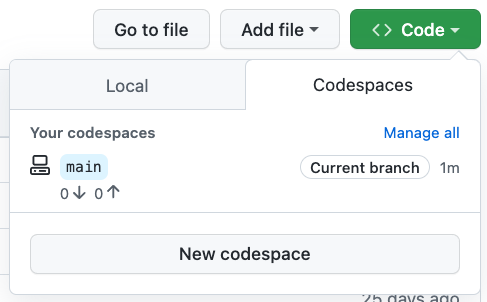
Today, the ability to prebuild codespaces is entering public beta. Prebuilding a codespace enables fast environment creation times, regardless of the size or complexity of your repositories. A prebuilt codespace will serve as a “ready-to-go” template where your source code, editor extensions, project dependencies, commands, and configurations have already been downloaded, installed, and applied so that you don’t have to wait for these tasks to finish each time you create a new codespace.
Getting to public beta
Our primary goal with Codespaces is to provide a one-click onboarding solution that enables developers to get started on a project quickly without performing any manual setup. However, because a codespace needs to clone your repository and (optionally) build a custom Dockerfile, install project dependencies and editor extensions, initialize scripts, and so on in order to bootstrap the development environment, there can be significant variability in the startup times that developers actually experience. A lot of this depends on the repository size and the complexity of a configuration.
Prebuilds were a huge part of how we meaningfully reduced the time-to-bootstrap in Codespaces for our core GitHub.com codebase. With that, our next mission was to replicate this success and enable the experience for our customers. Over the past few months, we ran a private preview for prebuilds with approximately 50 organizations. Overall, we received positive feedback on the ability of prebuilds to improve productivity for teams working on complex projects. At the same time, we also received a ton of valuable feedback around the configuration and management of prebuilds, and we’re excited to share those improvements with you today:
You can now identify and quickly get started with a fast create experience by selecting machine types that have a “prebuild ready” tag.
A seamless configuration experience helps repository admins easily set up and manage prebuild configurations for different branches and regions.
To reduce the burden on repository admins around managing Action version updates for each prebuilt branch, we introduced support for GitHub Actions workflows that will be managed by the Codespaces service.
Prebuild configurations are now built on GitHub Actions virtual machines. This enables faster prebuild template creations for each push made to your repository, and also provides repository admins with access to a rich set of logs to help with efficient debugging in case failures occur.
Our goal is to keep iterating on this experience based on the feedback captured during public beta and to continue our mission of enabling a seamless developer onboarding experience.
So how do prebuilds work?
During public beta, repository admins will be able to create prebuild configurations for specific branches and region(s) in their repository.
Prebuild configurations will automatically trigger an associated GitHub Actions workflow, managed by the Codespaces service, that will take care of prebuilding the devcontainer configuration and any subsequent commits for that branch. Associated prebuild templates will be stored in blob storage for each of the selected regions.
Each workflow will provide a rich set of logs to help with debugging in case failures occur.
Every time you request a prebuilt codespace, the service will fetch a prebuilt template and attach it to an existing virtual machine, thus significantly reducing your codespace creation time. To request changes to the prebuild configuration for your branch as per your needs, you can always update its associated devcontainer configuration with a pull request, specifically using the onCreateCommand or updateContentCommand lifecycle scripts.
How to get started
Prebuilds are available to try in public beta for all organizations that are a part of GitHub Enterprise Cloud and Team plans. As an organization or repository admin, you can head over to your repository’s settings page and create prebuild configurations under the “Codespaces” tab. As a developer, you can create a prebuilt codespace by heading over to a prebuild-enabled branch in your repository and selecting a machine type that has the “prebuild ready” label on it.
In large organisations, it is a common practice to isolate the cloud resources of different verticals. Amazon Web Services (AWS) Virtual Private Cloud (VPC) is a convenient way of doing so. At Grab, while our core AWS services reside in a main VPC, a number of Grab Tech Families (TFs) have their own dedicated VPC. One such example is GrabKios. Previously known as “Kudo”, GrabKios was acquired by Grab in 2017 and has always been residing in its own AWS account and dedicated VPC.
In this article, we explore how we exposed an Apache Kafka cluster across multiple Availability Zones (AZs) in Grab’s main VPC, to producers and consumers residing in the GrabKios VPC, via a VPC Endpoint Service. This design is part of Coban unified stream processing platform at Grab.
There are several ways of enabling communication between applications across distinct VPCs; VPC peering is the most straightforward and affordable option. However, it potentially exposes the entire VPC networks to each other, needlessly increasing the attack surface.
Security has always been one of Grab’s top concerns and with Grab’s increasing growth, there is a need to deprecate VPC peering and shift to a method of only exposing services that require remote access. The AWS VPC Endpoint Service allows us to do exactly that for TCP/IPv4 communications within a single AWS region.
Setting up a VPC Endpoint Service compared to VPC peering is already relatively complex. On top of that, we need to expose an Apache Kafka cluster via such an endpoint, which comes with an extra challenge. Apache Kafka requires clients, called producers and consumers, to be able to deterministically establish a TCP connection to all brokers forming the cluster, not just any one of them.
Last but not least, we need a design that optimises performance and cost by limiting data transfer across AZs.
Note: All variable names, port numbers and other details used in this article are only used as examples.
Architecture overview
As shown in this diagram, the Kafka cluster resides in the service provider VPC (Grab’s main VPC) while local Kafka producers and consumers reside in the service consumer VPC (GrabKios VPC).
In Grab’s main VPC, we created a Network Load Balancer (NLB) and set it up across all three AZs, enabling cross-zone load balancing. We then created a VPC Endpoint Service associated with that NLB.
Next, we created a VPC Endpoint Network Interface in the GrabKios VPC, also set up across all three AZs, and attached it to the remote VPC endpoint service in Grab’s main VPC. Apart from this, we also created a Route 53 Private Hosted Zone .grab and a CNAME record kafka.grab that points to the VPC Endpoint Network Interface hostname.
Lastly, we configured producers and consumers to use kafka.grab:10000 as their Kafka bootstrap server endpoint, 10000/tcp being an arbitrary port of our choosing. We will explain the significance of these in later sections.
Network Load Balancer setup
On the NLB in Grab’s main VPC, we set up the corresponding bootstrap listener on port 10000/tcp, associated with a target group containing all of the Kafka brokers forming the cluster. But this listener alone is not enough.
As mentioned earlier, Apache Kafka requires producers and consumers to be able to deterministically establish a TCP connection to all brokers. That’s why we created one listener for every broker in the cluster, incrementing the TCP port number for each new listener, so each broker endpoint would have the same name but with different port numbers, e.g. kafka.grab:10001 and kafka.grab:10002.
We then associated each listener with a dedicated target group containing only the targeted Kafka broker, so that remote producers and consumers could differentiate between the brokers by their TCP port number.
The following listeners and associated target groups were set up on the NLB:
In the Kafka brokers’ Security Group (SG), we added an ingress SG rule allowing 9094/tcp traffic from each of the three private IP addresses of the NLB. As mentioned earlier, the NLB was set up across all three AZs, with each having its own private IP address.
On the GrabKios VPC (consumer side), we created a new SG and attached it to the VPC Endpoint Network Interface. We also added ingress rules to allow all producers and consumers to connect to tcp/10000-10003.
Kafka setup
Kafka brokers typically come with a listener on port 9092/tcp, advertising the brokers by their private IP addresses. We kept that default listener so that local producers and consumers in Grab’s main VPC could still connect directly.
$ kcat -L -b 10.0.0.1:9092
 3 brokers:
 broker 101 at 10.0.0.1:9092 (controller)
 broker 201 at 10.0.0.2:9092
 broker 301 at 10.0.0.3:9092
... truncated output ...
We also configured all brokers with an additional listener on port 9094/tcp that advertises the brokers by:
Their shared private name kafka.grab.
Their distinct TCP ports previously set up on the NLB’s dedicated listeners.
$ kcat -L -b 10.0.0.1:9094
 3 brokers:
 broker 101 at kafka.grab:10001 (controller)
 broker 201 at kafka.grab:10002
 broker 301 at kafka.grab:10003
... truncated output ...
Note that there is a difference in how the broker’s endpoints are advertised in the two outputs above. The latter enables connection to any particular broker from the GrabKios VPC via the VPC Endpoint Service.
It would definitely be possible to advertise the brokers directly with the remote VPC Endpoint Interface hostname instead of kafka.grab, but relying on such a private name presents at least two advantages.
First, it decouples the Kafka deployment in the service provider VPC from the infrastructure deployment in the service consumer VPC. Second, it makes the Kafka cluster easier to expose to other remote VPCs, should we need it in the future.
Limiting data transfer across Availability Zones
At this stage of the setup, our Kafka cluster is fully reachable from producers and consumers in the GrabKios VPC. Yet, the design is not optimal.
When a producer or a consumer in the GrabKios VPC needs to connect to a particular broker, it uses its individual endpoint made up of the shared name kafka.grab and the broker’s dedicated TCP port.
The shared name arbitrarily resolves into one of the three IP addresses of the VPC Endpoint Network Interface, one for each AZ.
Hence, there is a fair chance that the obtained IP address is neither in the client’s AZ nor in that of the target Kafka broker. The probability of this happening can be as high as 2/3 when both client and broker reside in the same AZ and 1/3 when they do not.
While that is of little concern for the initial bootstrap connection, it becomes a serious drawback for actual data transfer, impacting the performance and incurring unnecessary data transfer cost.
For this reason, we created three additional CNAME records in the Private Hosted Zone in the GrabKios VPC, one for each AZ, with each pointing to the VPC Endpoint Network Interface zonal hostname in the corresponding AZ:
kafka-az1.grab
kafka-az2.grab
kafka-az3.grab
Note that we used az1, az2, az3 instead of the typical AWS 1a, 1b, 1c suffixes, because the latter’s mapping is not consistent across AWS accounts.
We also reconfigured each Kafka broker in Grab’s main VPC by setting their 9094/tcp listener to advertise brokers by their new zonal private names.
$ kcat -L -b 10.0.0.1:9094
 3 brokers:
 broker 101 at kafka-az1.grab:10001 (controller)
 broker 201 at kafka-az2.grab:10002
 broker 301 at kafka-az3.grab:10003
... truncated output ...
Our private zonal names are shared by all brokers in the same AZ while TCP ports remain distinct for each broker. However, this is not clearly shown in the output above because our cluster only counts three brokers, one in each AZ.
The previous common name kafka.grab remains in the GrabKios VPC’s Private Hosted Zone and allows connections to any broker via an arbitrary, likely non-optimal route. GrabKios VPC producers and consumers still use that highly-available endpoint to initiate bootstrap connections to the cluster.
Future improvements
For this setup, scalability is our main challenge. If we add a new broker to this Kafka cluster, we would need to:
Assign a new TCP port number to it.
Set up a new dedicated listener on that TCP port on the NLB.
Configure the newly spun up Kafka broker to advertise its service with the same TCP port number and the private zonal name corresponding to its AZ.
Add the new broker to the target group of the bootstrap listener on the NLB.
Update the network SG rules on the service consumer side to allow connections to the newly allocated TCP port.
We rely on Terraform to dynamically deploy all AWS infrastructure and on Jenkins and Ansible to deploy and configure Apache Kafka. There is limited overhead but there are still a few manual actions due to a lack of integration. These include transferring newly allocated TCP ports and their corresponding EC2 instances’ IP addresses to our Ansible inventory, commit them to our codebase and trigger a Jenkins job deploying the new Kafka broker.
Another concern of this setup is that it is only applicable for AWS. As we are aiming to be multi-cloud, we may need to port it to Microsoft Azure and leverage the Azure Private Link service.
In both cases, running Kafka on Kubernetes with the Strimzi operator would be helpful in addressing the scalability challenge and reducing our adherence to one particular cloud provider. We will explain how this solution has helped us address these challenges in a future article.
Special thanks to David Virgil Naranjo whose blog post inspired this work.
Join us
Grab is a leading superapp in Southeast Asia, providing everyday services that matter to consumers. More than just a ride-hailing and food delivery app, Grab offers a wide range of on-demand services in the region, including mobility, food, package and grocery delivery services, mobile payments, and financial services across over 400 cities in eight countries.
Powered by technology and driven by heart, our mission is to drive Southeast Asia forward by creating economic empowerment for everyone. If this mission speaks to you, join our team today!
GitHub code scanning now uses machine learning (ML) to alert developers to potential security vulnerabilities in their code.
If you want to set up your repositories to surface more alerts using our new ML technology, get started here. Read on for a behind-the-scenes peek into the ML framework powering this new technology!
Detecting vulnerable code
Code security vulnerabilities can allow malicious actors to manipulate software into behaving in unintended and harmful ways. The best way to prevent such attacks is to detect and fix vulnerable code before it can be exploited. GitHub’s code scanning capabilities leverage the CodeQL analysis engine to find security vulnerabilities in source code and surface alerts in pull requests – before the vulnerable code gets merged and released.
To detect vulnerabilities in a repository, the CodeQL engine first builds a database that encodes a special relational representation of the code. On that database we can then execute a series of CodeQL queries, each of which is designed to find a particular type of security problem.
Many vulnerabilities are caused by a single repeating pattern: untrusted user data is not sanitized and is subsequently accidentally used in an unsafe way. For example, SQL injection is caused by using untrusted user data in a SQL query, and cross-site scripting occurs as a result of untrusted user data being written to a web page. To detect situations in which unsafe user data ends up in a dangerous place, CodeQL queries encapsulate knowledge of a large number of potential sources of user data (for example, web frameworks), as well as potentially risky sinks (such as libraries for executing SQL queries). Members of the security community, alongside security experts at GitHub, continually expand and improve these queries to model additional common libraries and known patterns. Manual modeling, however, can be time-consuming, and there will always be a long tail of less-common libraries and private code that we won’t be able to model manually. This is where machine learning comes in.
We use examples surfaced by the manual models to train deep learning neural networks that can determine whether a code snippet comprises a potentially risky sink.
As a result, we can uncover security vulnerabilities even when they arise from the use of a library we have never seen before. For example, we can detect SQL injection vulnerabilities in the context of lesser-known or closed-source database abstraction libraries.
ML-powered queries generate alerts that are marked with the “Experimental” label
Building a training set
We need to train ML models to recognize vulnerable code. While we have experimented some with unsupervised learning, unsurprisingly we found that supervised learning works better. But it comes at a cost! Asking code security experts to manually label millions of code snippets as safe or vulnerable is clearly untenable. So where do we get the data?
The manually written CodeQL queries already embody the expertise of the many security experts who wrote and refined them. We leverage these manual queries as ground-truth oracles, to label examples we then use to train our models. Each sink detected by such a query serves as a positive example in the training set. Since the vast majority of code snippets do not contain vulnerabilities, snippets not detected by the manual models can be regarded as negative examples. We make up for the inherent noise in this inferred labeling with volume. We extract tens of millions of snippets from over a hundred thousand public repositories, run the CodeQL queries on them, and label each as a positive or negative example for each query. This becomes the training set for a machine learning model that can classify code snippets as vulnerable or not.
Of course, we don’t want to train a model that will simply reproduce the manual modeling; we want to train a model that will predict new vulnerabilities that weren’t captured by manual modeling. In effect, we want the ML algorithm to improve on the current version of the manual query in much the same way that the current version improves on older, less-comprehensive versions. To see if we can do this, we actually construct all our training data from an older version of the query that detects fewer vulnerabilities. We then apply the trained model to new repositories it wasn’t trained on. We measure how well we recover the alerts detected by the latest manual query but missed by the older version of the query. This allows us to simulate the ability of a model trained with the current version of the query to recover alerts missed by this current manual model.
Features and modeling
Given a large training set of code snippets labeled as positive or negative examples for each query, we extract features for each snippet and train a deep learning model to classify new examples.
Rather than treating each code snippet simply as a string of words or characters and applying standard natural language processing (NLP) techniques naively to classify these strings, we leverage the power of CodeQL to access a wealth of information about the underlying source code. We use this information to produce a rich set of highly informative features for each code snippet.
One of the main advantages of deep learning models is their ability to combine information from a large set of features to create higher-level features and discover patterns that aren’t obvious to humans. In partnership with security and programming-language experts at GitHub, we use CodeQL to extract the information an expert might examine to inform a decision, such as the entire enclosing function body for a snippet that sits within a function, or the access path and API name. We don’t have to limit ourselves to features a human would find informative, however. We can include features whose usefulness is unknown, or features that can be useful in some instances but not all, such as the argument index for a code snippet that’s an argument to a function. Such features may contain patterns that aren’t apparent to humans, but that the neural network can detect. We therefore let the machine learning model decide whether or how to use all these features, and how to combine them to make the best decision for each snippet.
Once we’ve extracted a rich set of potentially interesting features for each example, we tokenize and sub-tokenize them as is commonly done in NLP applications, with some modifications to capture characteristics specific to code syntax. We generate a vocabulary from the training data and feed lists of indices into the vocabulary into a fairly simple deep learning classifier, with a few layers of feature-by-feature processing followed by concatenation across features and a few layers of combined processing. The output is the probability that the current sample is a vulnerability for each query type.
Due to the scale of our offline data labeling, feature extraction, and training pipelines, we leverage cloud compute, including GPUs for model training. At inference time, however, no GPU is needed.
Inference on a repository
Once we have our trained machine learning model, we use it to classify new code snippets and detect likely vulnerabilities for each query. When ML-generated alerts are enabled by repository owners, CodeQL computes the source code features for the code snippets in that codebase and feeds them into the classifier model. The framework gets back the probability that a given code snippet represents a vulnerability, and uses this probability to surface likely new alerts.
The full process runs on the same standard GitHub Action runners that are used by code scanning more generally, and it’s transparent to the user other than some increased runtime on large repositories. When the code scanning is complete, users can see the ML-generated alerts along with the alerts surfaced by the manual queries, with the “Experimental” label allowing them to filter ML-generated alerts in or out.
Does it work?
When evaluating ML-generated alerts, we consider only new alerts that were not flagged by the manual queries. True positives are the correct alerts that were missed by the manual queries; false positives are the incorrect new alerts generated by the ML model.
To measure metrics at scale, we use the experimental setup described above, in which the labels in the training set are determined using an older version of each manual query. We then test the model on repositories that were not included in the training set, and we measure its ability to recover the alerts detected by the current manual query but missed by the older one. Our metrics vary by query, but on average we measure a recall of approximately 80% with a precision of approximately 60%.
We’re currently extending ML-generated alerts to more JavaScript and Typescript security queries, as well as working to improve both their performance and their runtime. Our future plans include expansion to more programming languages, as well as generalizations that will allow us to capture even more vulnerabilities.
Run the “Experimental” queries if you want to uncover more potential security vulnerabilities in your codebase. The more the community engages with our alerts and provides feedback, the better we can make our algorithms, so please consider giving them a try!
A picture tells a thousand words, but up until now the only way to include pictures and diagrams in your Markdown files on GitHub has been to embed an image. We added support for embedding SVGs recently, but sometimes you want to keep your diagrams up to date with your docs and create something as easily as doing ASCII art, but a lot prettier.
Enter Mermaid
Mermaid is a JavaScript based diagramming and charting tool that takes Markdown-inspired text definitions and creates diagrams dynamically in the browser. Maintained by Knut Sveidqvist, it supports a bunch of different common diagram types for software projects, including flowcharts, UML, Git graphs, user journey diagrams, and even the dreaded Gantt chart.
Working with Knut and also the wider community at CommonMark, we’ve rolled out a change that will allow you to create graphs inline using Mermaid syntax, for example:
The raw code block above will appear as this diagram in the rendered Markdown:
How it works
When we encounter code blocks marked as mermaid, we generate an iframe that takes the raw Mermaid syntax and passes it to Mermaid.js, turning that code into a diagram in your local browser.
We achieve this through a two-stage process—GitHub’s HTML pipeline and Viewscreen, our internal file rendering service.
First, we add a filter to the HTML pipeline that looks for raw pre tags with the mermaid language designation and substitutes it with a template that works progressively, such that clients requesting content with embedded Mermaid in a non-JavaScript environment (such as an API request) will see the original Markdown code.
Next, assuming the content is viewed in a JavaScript-enabled environment, we inject an iframe into the page, pointing the src attribute to the Viewscreen service. This has several advantages:
It offloads the library to an external service, keeping the JavaScript payload we need to serve from Rails smaller.
Rendering the charts asynchronously helps eliminate the overhead of potentially rendering several charts before sending the compiled ERB view to the client.
User-supplied content is locked away in an iframe, where it has less potential to cause mischief on the GitHub page that the chart is loaded into.
The net result is fast, easily editable, and vector-based diagrams right in your documentation where you need them.
Mermaid has been getting increasingly popular with developers and has a rich community of contributors led by the maintainer Knut Sveidqvist. We are very grateful for Knut’s support in bringing this feature to everyone on GitHub. If you’d like to learn more about the Mermaid syntax, head over to the Mermaid website or check out Knut’s first official Mermaid book.
GrabAds is a service that provides businesses with an opportunity to market their products to Grab’s consumer base. During the pandemic, as the demand for food delivery grew, we realised that ads could be a service we offer to our small restaurant merchant-partners to expand their reach. This would allow them to not only mitigate the loss of in-person traffic but also grow by attracting more customers.
Many of these small merchant-partners had no experience with digital advertising and we provided an easy-to-use, scalable option that could match their business size. On the other side of the equation, our large network of merchant-partners provided consumers with more choices. For hungry consumers stuck at home, personalised ads and promotions helped them satisfy their cravings, thus fulfilling their intent of opening the Grab app in the first place!
Why build our own ad server?
Building an ad server is an ambitious undertaking and one might rightfully ask why we should invest the time and effort to build a technically complex distributed system when there are several reasonable off-the-shelf solutions available.
The answer is we didn’t, at least not at first. We used one of these off-the-shelf solutions to move fast and build a minimally viable product (MVP). The result of this experiment was a resounding success; we were providing clear value to our merchant-partners, our consumers and Grab’s overall business.
However, to take things to the next level meant scaling the ads business up exponentially. Apart from being one of the few companies with the user engagement to support an ads business at scale, we also have an ecosystem that combines our network of merchant-partners, an understanding of our consumers’ interactions across multiple services in the Grab superapp, and a payments solution, GrabPay, to close the loop. Furthermore, given the hyperlocal nature of our business, the in-app user experience is highly customised by location. In order to integrate seamlessly with this ecosystem, scale as Grab’s overall business grows and handle personalisation using machine learning (ML), we needed an in-house solution.
What we built
We designed and built a set of microservices, streams and pipelines which orchestrated the core ad serving functionality, as shown below.
Targeting – This is the first step in the ad serving flow. We fetch a set of candidate ads specifically targeted to the request based on keywords the user searched for, the user’s location, the time of day, and the data we have about the user’s preferences or other characteristics. We chose ElasticSearch as the data store for our ads repository as it allows us to query based on a disparate set of targeting criteria.
Capping – In this step, we filter out candidate ads which have exceeded various caps. This includes cases where an advertising campaign has already reached its budget goal, as well as custom requirements about the frequency an ad is allowed to be shown to the same user. In order to make this decision, we need to know how much budget has already been spent and how many times an ad has already been shown. We chose ScyllaDB to store these “stats”, which is scalable, low-cost and can handle the large read and write requirements of this process (more on how this data gets written to ScyllaDB in the Tracking step).
Pacing – In this step, we alter the probability that a matching ad candidate can be served, based on a specific campaign goal. For example, in some cases, it is desirable for an ad to be shown evenly throughout the day instead of exhausting the entire ad budget as soon as possible. Similar to Capping, we require access to information on how many times an ad has already been served and use the same ScyllaDB stats store for this.
Scoring – In this step, we score each ad. There are a number of factors that can be used to calculate this score including predicted clickthrough rate (pCTR), predicted conversion rate (pCVR) and other heuristics that represent how relevant an ad is for a given user.
Ranking – This is where we compare the scored candidate ads with each other and make the final decision on which candidate ads should be served. This can be done in several ways such as running a lottery or performing an auction. Having our own ad server allows us to customise the ranking algorithm in countless ways, including incorporating ML predictions for user behaviour. The team has a ton of exciting ideas on how to optimise this step and now that we have our own stack, we’re ready to execute on those ideas.
Pricing – After choosing the winning ads, the final step before actually returning those ads in the API response is to determine what price we will charge the advertiser. In an auction, this is called the clearing price and can be thought of as the minimum bid price required to outbid all the other candidate ads. Depending on how the ad campaign is set up, the advertiser will pay this price if the ad is seen (i.e. an impression occurs), if the ad is clicked, or if the ad results in a purchase.
Tracking – Here, we close the feedback loop and track what users do when they are shown an ad. This can include viewing an ad and ignoring it, watching a video ad, clicking on an ad, and more. The best outcome is for the ad to trigger a purchase on the Grab app. For example, placing a GrabFood order with a merchant-partner; providing that merchant-partner with a new consumer. We track these events using a series of API calls, Kafka streams and data pipelines. The data ultimately ends up in our ScyllaDB stats store and can then be used by the Capping and Pacing steps above.
Principles
In addition to all the usual distributed systems best practices, there are a few key principles that we focused on when building our system.
Latency – Latency is important for ads. If the user scrolls faster than an ad can load, the ad won’t be seen. The longer an ad remains on the screen, the more likely the user will notice it, have their interest piqued and click on it. As such, we set strict limits on the latency of the ad serving flow. We spent a large amount of effort tuning ElasticSearch so that it could return targeted ads in the shortest amount of time possible. We parallelised parts of the serving flow wherever possible and we made sure to A/B test all changes both for business impact and to ensure they did not increase our API latency.
Graceful fallbacks – We need user-specific information to make personalised decisions about which ads to show to a given user. This data could come in the form of segmentation of our users, attributes of a single user or scores derived from ML models. All of these require the ad server to make dependency calls that could add latency to the serving flow. We followed the principle of setting strict timeouts and having graceful fallbacks when we can’t fetch the data needed to return the most optimal result. This could be due to network failures or dependencies operating slower than usual. It’s often better to return a non-personalised result than no result at all.
Global optimisation – Predicting supply (the amount of users viewing the app) and demand (the amount of advertisers wanting to show ads to those users) is difficult. As a superapp, we support multiple types of ads on various screens. For example, we have image ads, video ads, search ads, and rewarded ads. These ads could be shown on the home screen, when booking a ride, or when searching for food delivery. We intentionally decided to have a single ad server supporting all of these scenarios. This allows us to optimise across all users and app locations. This also ensures that engineering improvements we make in one place translate everywhere where ads or promoted content are shown.
What’s next?
Grab’s ads business is just getting started. As the number of users and use cases grow, ads will become a more important part of the mix. We can help our merchant-partners grow their own businesses while giving our users more options and a better experience.
Some of the big challenges ahead are:
Optimising our real-time ad decisions, including exciting work on using ML for more personalised results. There are many factors that can be considered in ad personalisation such as past purchase history, the user’s location and in-app browsing behaviour. Another area of optimisation is improving our auction strategy to ensure we have the most efficient ad marketplace possible.
Expanding the types of ads we support, including experimenting with new types of content, finding the best way to add value as Grab expands its breadth of services.
Scaling our services so that we can match Grab’s velocity and handle growth while maintaining low latency and high reliability.
Join us
Grab is a leading superapp in Southeast Asia, providing everyday services that matter to consumers. More than just a ride-hailing and food delivery app, Grab offers a wide range of on-demand services in the region, including mobility, food, package and grocery delivery services, mobile payments, and financial services across over 400 cities in eight countries.
Powered by technology and driven by heart, our mission is to drive Southeast Asia forward by creating economic empowerment for everyone. If this mission speaks to you, join our team today!
In January, we experienced no incidents resulting in service downtime to our core services. However, we do want to acknowledge an incident in February that we are continuing to investigate.
February 2 19:12 UTC (lasting 26 minutes)
Our service monitors detected a high rate of errors for issues, pull requests, GitHub Codespaces, and GitHub Actions services. We have mitigated the incident and are confident it has been fully resolved.
Due to the recency of this incident, we are still investigating the contributing factors and will provide a more detailed update in next month’s report.
We recently added beta support for Ruby to the CodeQL engine that powers GitHub code scanning, as part of our efforts to make it easier for developers to build and ship secure code. Ruby support is particularly exciting for us, since GitHub itself is a Ruby on Rails app. Any improvements we or the community make to CodeQL’s vulnerability detection will help secure our own code, in addition to helping Ruby’s open source ecosystem.
CodeQL’s static analysis works by running queries over a database representation of a program. The following diagram gives a high-level overview of the process:
While there’s plenty I’d love to tell you about how we write queries, and about our rich set of analysis libraries, I’m going to focus in this post on how we build those databases: how we’ve typically done it for other languages and how we did things a little differently for Ruby.
Introducing the extractor
If you want to be able to create databases for a new language in CodeQL, you need to write an extractor. An extractor is a tool that:
parses the source code to obtain a parse tree,
converts that parse tree into a relational form, and
writes those relations (database tables) to disk.
You also need to define a schema for the database produced by your extractor. The schema specifies the names of tables in the database and the names and types of columns in each table.
Let’s visit parse trees, parsers, and database schemas in more detail.
Parse trees
Source code is just text. If you’re writing a compiler, performing static analysis, or even just doing syntax highlighting, you want to convert that text to a structure that is easier to work with. The structure we use is a parse tree, also known as a concrete syntax tree.
Here’s a friendly little Ruby program that prints a couple of greetings:
puts("Hello", "Ahoy")
The program contains three expressions: the string literals "Hello" and "Ahoy" and a call to a method named puts. I could draw a minimal parse tree for the program like this:
Compilers and static analysis tools like CodeQL often convert the parse tree into a simpler format known as an abstract syntax tree (AST), so-called because it abstracts away some of the syntactic details that do not affect the meaning of the program, such as comments, whitespace, and parentheses. If I wanted – and if I assume that puts is a method built into the language – I could write a simple interpreter that executes the program by walking the AST.
For CodeQL, the Ruby extractor stores the parse tree in the database, since those syntactic details can sometimes be useful. We then provide a query library to transform this into an AST, and most of our queries and query libraries build on top of that transformed AST, either directly or after applying further transformations (such as the construction of a data-flow graph).
Choosing a parser
For each language we’ve supported so far, we’ve used a different parser, choosing the one that gives the best performance and compatibility across all the codebases we want to analyze. For example, our C# extractor parses C# source code using Microsoft’s open source Roslyn compiler, while our JavaScript extractor uses a parser that was derived from the Acorn project.
For Ruby, we decided to use tree-sitter and its Ruby parser. Tree-sitter is a parser framework developed by our friends in GitHub’s Semantic Code Team and is the technology underlying the syntax highlighting and code navigation (jump-to-definition) features on GitHub.com.
Tree-sitter is fast, has excellent error recovery, and provides bindings for several languages (we chose to use the Rust bindings, which are particularly pleasant). It has parsers not only for Ruby, but for most other popular languages, and provides machine-readable descriptions of each language’s grammar. These opened up some exciting possiblities for us, which I’ll describe later.
In practice, the parse tree produced by tree-sitter for our example program is a little more complicated than the diagram above (for one thing, string literal nodes have child nodes in order to support string interpolation). If you’re curious, you can go to the tree-sitter playground, select Ruby from the dropdown, and try it for yourself.
Handling ambiguity
Ruby has a flexible syntax that delights (most of) the people who program in it. The word ‘elegant’ gets thrown around a lot, and Ruby programs often read more like English prose than code. However, this elegance comes at a significant cost: the language is ambiguous in several places, and dealing with it in a parser creates a lot of complexity.
Ruby is simple in appearance, but is very complex inside, just like our human body.
– Yukihiro 'Matz' Matsumoto, Ruby's creator
Matz’s Ruby Interpreter (MRI) is the canonical implementation of the Ruby language, and its parser is implemented in the file parse.y (from which Bison generates the actual parser code). That file is currently 14,000 lines long, which should give you a sense of the complexity involved in parsing Ruby.
One interesting example of Ruby’s ambiguity occurs when parsing an unadorned identifier like foo. If it had parentheses – foo() – we could parse it unambiguously as a method call, but parentheses are optional in Ruby. Is foo a method call with zero arguments, or is it a variable reference? Well, that ultimately depends on whether a variable named foo is in scope. If so, it’s a variable reference; otherwise, we can assume it’s a call to a method named foo.
What type of parse-tree node should the parser return in this case? The parser does not track which variables are in scope, so it cannot decide. The way tree-sitter and the extractor handle this is to emit an identifier node rather than a call node. It’s only later, as we evaluate queries, that our AST library builds a control-flow graph of the program and uses that to decide whether the node is a method call or a variable reference.
Representing a parse tree in a relational database
While the parse trees produced by most parser libraries typically represent nodes and edges in the tree as objects and pointers, CodeQL uses a relational database. Going back to the simple diagram above, I can attempt to convert it to relational form. To do that, I should first define a schema (in a simplified version of CodeQL’s schema syntax):
The expressions table has a row for each expression in the program. Each one is given a unique id, a primary key that I can use to reference the expression from other tables. The kind column defines what kind of expression it is. I can decide that a value of 1 means the expression is a method call, 2 means it’s a string literal, and so on.
The calls table has a row for each method call, and it allows me to specify data that is specific to call expressions. The first column is a foreign key, i.e. the id of the corresponding entry in the expressions table, while the second column specifies the name of the method. You might have expected that I’d add columns for the call’s arguments, but calls can take any number of arguments, so I wouldn’t know how many columns to add. Instead, I put them in a separate call_arguments table.
The call_arguments table, therefore, has one row per argument in the program. It has three columns: one that’s a reference to the call expression, another that’s a reference to an argument, and a third that specifies the index, or number, of that argument.
Finally, the string_literals table lets me associate the literal text value with the corresponding entry in the expressions table.
Populating our small database
Now that I’ve defined my schema, I’m going to manually populate a matching database with rows for my little greeting program:
expressions
id
kind
100
1 (call)
101
2 (string literal)
102
2 (string literal)
calls
expr_id
name
100
“puts”
call_arguments
call_id
arg_id
arg_index
100
101
0
100
102
1
string_literals
expr_id
val
101
“Hello”
102
“Ahoy”
Suppose this were a SQL database, and I wanted to write a query to find all the expressions that are arguments in calls to the puts method. It might look like this:
SELECT call_arguments.arg_id
FROM call_arguments
INNER JOIN calls ON calls.expr_id = call_arguments.call_id
WHERE calls.name = "puts";
In practice, we don’t use SQL. Instead, CodeQL queries are written in the QL language and evaluated using our custom database engine. QL is an object-oriented, declarative logic-programming language that is superficially similar to SQL but based on Datalog. Here’s what the same query might look like in QL:
from MethodCall call, Expr arg
where
  call.getMethodName() = "puts" and
  arg = call.getAnArgument()
select arg
MethodCall and Expr are classes that wrap the database tables, providing a high-level, object-oriented interface, with helpful predicates like getMethodName() and getAnArgument().
Language-specific schemas
The toy database schema I defined might look as though it could be reused for just about every programming language that has string literals and method calls. However, in practice, I’d need to extend it to support some features that are unique to Ruby, such as the optional blocks that can be passed with every method call.
Every language has these unique quirks, so each one GitHub supports has its own schema, perfectly tuned to match that language’s syntax. Whereas my toy schema had only two kinds of expression, our JavaScript and C/C++ schemas, for example, both define over 100 kinds of expression. Those schemas were written manually, being refined and expanded over the years as we made improvements and added support for new language features.
In contrast, one of the major differences in how we approached Ruby is that we decided to generate the database schema automatically. I mentioned earlier that tree-sitter provides a machine-readable description of its grammar. This is a file called node-types.json, and it provides information about all the nodes tree-sitter can return after parsing a Ruby program. It defines, for example, a type of node named binary, representing binary operation expressions, with fields named left, operator, and right, each with their own type information. It turns out this is exactly the kind of information we want in our database schema, so we built a tool to read node-types.json and spit out a CodeQL database schema.
I’ve talked about how the parser gives us a parse tree, and how we could represent that same tree in a database. That’s really the main job of an extractor – massaging the parse tree into a relational database format. How easy or difficult that is depends a lot on how similar those two structures look. For some languages, we defined our database schema to closely match the structure (and naming scheme) of the tree produced by the parser. That is, there’s a high level of correspondence between the parser’s node names and the database’s table names. For those languages, an extractor’s job is fairly simple. For other languages, where we perhaps decided that the tree produced by the parser didn’t map nicely to our ideal database schema, we have to do more work to convert from one to the other.
For Ruby, where we wrote a schema-generator to automatically translate tree-sitter’s description of its node types, our extractor’s job is quite simple: when tree-sitter parses the program and gives us those tree nodes, we can perform the same translations and automatically produce a database that conforms to the schema.
Language independence
This extraction process is not only straightforward, it’s also completely language-agnostic. That is, the process is entirely mechanical and works for any tree-sitter grammar. Our schema-generator and extractor know nothing about Ruby or its syntax – they simply know how to translate tree-sitter’s node-types.json. Since tree-sitter has parsers for dozens of languages, and they all have corresponding node-types.json files, we have effectively written a pair of tools that could produce CodeQL databases for any of them.
One early benefit of this approach came when we realized that, to provide comprehensive analysis of Ruby on Rails applications, we’d also need to parse the ERB templates used to render Rails views. ERB is a distinct language that needs to be parsed separately and extracted into our database. Thankfully, tree-sitter has an existing ERB parser, so we simply had to point our tooling at that node-types.json file as well, and suddenly we had a schema-generator and extractor that could handle both Ruby and ERB.
As an aside, the ERB language is quite simple, mostly consisting of tags that differentiate between the parts of the template that are text and the parts that are Ruby code. The ERB parser only cares about those tags and doesn’t parse the Ruby code itself. This is because tree-sitter provides an elegant feature that will return a series of byte offsets delimiting the parts that are Ruby code, which we can then pass on to the Ruby parser. So, when we extract an ERB file, we parse and extract the ERB parse tree first, and then perform a second pass that parses and extracts the Ruby parse tree, ignoring the text parts of the template file.
Of course, this automated approach to extraction does come with some tradeoffs, since it involves deferring some work from the extraction stage to the analysis stage. Our QL AST library, for example, has to do more work to transform the parse tree into a user-friendly AST representation, compared with some languages where the AST classes are thin wrappers over database tables. And if we look at our existing extractor for C#, for example, we see that it gets type information from the Roslyn compiler frontend, and stores it in the database. Our language-independent tooling, meanwhile, does not attempt any kind of type analysis, so if we wanted to use it on a static language, we’d have to implement that type analysis ourselves in QL.
Nonetheless, we are excited about the possibilities this language-independent tooling opens up as we look to expand CodeQL analysis to cover more languages in the future, especially for dynamic languages. There’s a lot more to analyzing a language than producing a database, but getting that part working with little to no effort should be a major time-saver.
github/github: so good, they named it twice
github/github is the Ruby on Rails application that powers GitHub.com, and it’s rather large. I’ve heard it said that it’s one of the largest Rails apps in the world. That means it’s an excellent stress test for our Ruby extractor.
It was actually the second Ruby program we ever extracted (the first was “Hello, World!”).
Of course, extraction wasn’t quite perfect. We observed a number of parser errors that we fixed upstream in the tree-sitter-ruby project, so our work not only resulted in improved Ruby code-viewing on GitHub.com, but also improvements in the other projects that use tree-sitter, such as Neovim’s syntax highlighting.
It was also a useful benchmark in our goal of making extraction as fast as possible. CodeQL can’t start doing the valuable work of analyzing for vulnerabilities until the code has been extracted and a database produced, so we wanted to make this as fast as possible. It certainly helps that tree-sitter itself is fast, and that our automatic translation of tree-sitter’s parse tree is simple.
The biggest speedup – and where our choice to implement the extractor in Rust really helped – was in implementing multi-threaded extraction. With the design we chose for the Ruby extractor, the work it performs on each source file is completely independent of any other source file. That makes extraction an embarrassingly parallel problem, and using the Rayon library meant we barely had to change any code at all to take advantage of that. We simply changed a for loop to use a Rayon parallel-iterator, and it handled the rest. Suddenly extraction got eight times faster on my eight-core laptop.
CodeQL now runs on every pull request against github/github, using a 32-core Actions runner, where Ruby extraction takes just 15 seconds. The core engine still has to perform ‘database finalization’ after the extractor finishes, and this takes a little longer (it parallelizes, but not “embarrassingly”), but we are extremely pleased with the extractor’s performance given the size of the github/github codebase, and given our experiences with extracting other languages.
We should be in a good place to accommodate all our users’ Ruby codebases, large and small.
Try it out
I hope you’ve enjoyed this dive into the technical details of extracting CodeQL databases. If you’d like to try CodeQL on your Ruby projects, please refer to the blog post announcing the Ruby public beta, which contains several handy links to help you get started.
By Karen Casella, Director of Engineering, Access & Identity Management
Have you ever experienced one of the following scenarios while looking for your next role?
You study and practice coding interview problems for hours/days/weeks/months, only to be asked to merge two sorted lists.
You apply for multiple roles at the same company and proceed through the interview process with each hiring team separately, despite the fact that there is tremendous overlap in the roles.
You go through the interview process, do really well, get really excited about the company and the people you meet, and in the end, you are “matched” to a role that does not excite you, working with a manager and team you have not even met during the interview process.
Interviewing can be a daunting endeavor and how companies, and teams, approach the process varies greatly. We hope that by demystifying the process, you will feel more informed and confident about your interview experience.
Backend Engineering Interview Loop
When you apply for a backend engineering role at Netflix, or if one of our recruiters or hiring managers find your LinkedIn profile interesting, a recruiter or hiring manager reviews your technical background and experience to see if your experience is aligned with our requirements. If so, we invite you to begin the interview process.
Most backend engineering teams follow a process very similar to what is shown below. While this is a relatively stream-lined process, it is not as efficient if a candidate is interested in or qualified for multiple roles within the organization.
Following is a brief description of each of these stages.
Recruiter Phone Screen: A member of our talent team contacts you to explain the process and to assess high-level qualifications . The recruiter also reviews the relevant open roles to see if you have a strong affinity for one or another. If your interests and experience align well with one or more of the roles, they schedule a phone screen with one of the hiring managers.
Manager Phone Screen: The purpose of this discussion is to get a sense for your technical background, your approach to problem solving, and how you work. It’s also a great opportunity for you to learn more about the available roles, the technical challenges the teams are facing and what it’s like to work on a backend engineering team at Netflix.
Technical Screen: The final screen before on-site interviews is used to assess your technical skills and match for the team. For many roles, you will be given a choice between a take-home coding exercise or a one-hour discussion with one of the engineers from the team. The problems you are asked to solve are related to the work of the team.
Round 1 Interviews: If you are invited on-site, the first round interview is with four or five people for 45 minutes each. The interview panel consists of two or three engineers, a hiring manager and a recruiter. The engineers assess your technical skills by asking you to solve various design and coding problems. These questions reflect actual challenges that our teams face.
Round 2 Interviews: You meet with two or three additional people, for 45 minutes each. The interview panel comprises an engineering director, a partner engineer or manager, and another engineering leader. The focus of this round is to assess how well you partner with other teams and your non-technical skills.
Decision & Offer: After round 2, we review the feedback and decide whether or not we will be offering you a role. If so, you will work with the recruiter to discuss compensation expectations, answer any questions that remain for you, and discuss a start date with your new team.
Enter Centralized Hiring
Some Netflix backend engineering teams, seeking stunning colleagues with similar backgrounds and talents, are joining forces and adopting a centralized hiring model. Centralized hiring is an approach of making multiple hiring decisions through one unified hiring process across multiple teams with shared needs in skill, function and experience level.
The interview approach does not vary much from what is shown above, with one big exception: there are several potential “pivot points” where you and / or Netflix may decide to focus on a particular role based on your experience and preference. At each stage of the process, we consider your preference and skills and may focus your remaining interviews with a specific team if we both consider it a strong match. It’s important to note that, even though your experience may not be an exact match for one team, you might be more closely aligned with another team. In that case, we would pivot you to another team rather than disqualify you from the process.
Interview Tips
Interviewing can be intimidating and stressful! Being prepared can help you minimize stress and anxiety. Following are a few quick tips to help you prepare:
Review your profile and make connections between your experience and the job description.
Think about your past work experiences and prepare some examples of when you achieved something amazing, or had some tough challenges.
We recommend against interview coding practice puzzle-type exercises, as we don’t ask those types of questions. If you want to practice, focus on medium-difficulty real-world problems you might encounter in a software engineering role.
Be sure to have questions prepared to ask the interviewers. This is a conversation, not an inquisition!
We are here to accommodate any accessibility needs you may have, to ensure that you’re set up for success during your interview. Let us know if you need any assistive technology or other accommodations ahead of time, and we’ll be sure to work with you to get it set up.
We want to see you at your best — we are not trying to trick you or trip you up! Try to relax, remember to breathe, and be honest and curious. Remember, this is not just about whether Netflix thinks you are a fit for the role, it’s about you deciding that Netflix and the role are right for you!
Yes, We Are Hiring!
Several of our backend engineering teams are searching for our next stunning colleagues. Some of the areas for which we are actively seeking backend engineers include Streaming & Gaming Technologies, Product Innovation, Infrastructure, and Studio Technologies. If any of the high-level descriptions below are of interest to you and seem like a good match for your experience and career goals, we’d like to hear from you! Simply click on the job description link and submit your application through our jobs site.
You are a distributed systems engineer working on product backend systems that support streaming video and/or mobile & cloud games.
You’re passionate about resilience, scalability, availability, and observability. Passion for large data sets, APIs, access & identity management, or delivering backend systems that enable mobile and cloud gaming is a big plus.
Your work centers around architecting, building and operating fault-tolerant distributed systems at massive scale.
You are a distributed systems engineer working on core backend services that support our user journeys in signup, subscription, search, personalization and messaging.
You’re passionate about working at the intersection of business, product and technology at large scale.
Your work centers around building fault-tolerant backend systems and services that make a direct impact on users and the business.
You are a software engineer that builds products and services used by creative partners across the studio and external productions to produce and manage all of Netflix global content. Our products enable the entire workflow of content acquisition, production, promotion and financing from script to screen. We create innovative solutions that develop and manage entertainment at scale while helping entertain the world as members find joy in the shows and movies they love.
You’re passionate about innovation, scalability, functionality, shipping high-value features quickly and are committed to delivering exceptional backend systems for our consumers. You’re humble, curious, and looking to deliver results with other stunning colleagues.
Your work centers around building products and services targeting creative partners producing/managing global content.
Conclusion
Netflix has a Freedom & Responsibility culture in which every Netflix employee has the freedom to do their best work and the responsibility to achieve excellence. We value strong judgment, communication, impact, curiosity, innovation, courage, passion, integrity, selflessness, inclusion, and diversity. For more information on the culture, see http://jobs.netflix.com/culture.
Karen Casella is the Director of Engineering for Access & Identity Management technologies for Netflix streaming and gaming products. Connect with Karen on LinkedIn or Twitter.
The open source Git project just released Git 2.35, with features and bug fixes from over 93 contributors, 35 of them new. We last caught up with you on the latest in Git back when 2.34 was released. To celebrate this most recent release, here’s GitHub’s look at some of the most interesting features and changes introduced since last time.
When working on a complicated change, it can be useful to temporarily discard parts of your work in order to deal with them separately. To do this, we use the git stash tool, which stores away any changes to files tracked in your Git repository.
Using git stash this way makes it really easy to store all accumulated changes for later use. But what if you only want to store part of your changes in the stash? You could use git stash -p and interactively select hunks to stash or keep. But what if you already did that via an earlier git add -p? Perhaps when you started, you thought you were ready to commit something, but by the time you finished staging everything, you realized that you actually needed to stash it all away and work on something else.
git stash‘s new --staged mode makes it easy to stash away what you already have in the staging area, and nothing else. You can think of it like git commit (which only writes staged changes), but instead of creating a new commit, it writes a new entry to the stash. Then, when you’re ready, you can recover your changes (with git stash pop) and keep working.
git log has a rich set of --format options that you can use to customize the output of git log. These can be handy when sprucing up your terminal, but they are especially useful for making it easier to script around the output of git log.
In our blog post covering Git 2.33, we talked about a new --format specifier called %(describe). This made it possible to include the output of git describe alongside the output of git log. When it was first released, you could pass additional options down through the %(describe) specifier, like matching or excluding certain tags by writing --format=%(describe:match=<foo>,exclude=<bar>).
In 2.35, Git includes a couple of new ways to tweak the output of git describe. You can now control whether to use lightweight tags, and how many hexadecimal characters to use when abbreviating an object identifier.
You can try these out with %(describe:tags=<bool>) and %(describe:abbrev=<n>), respectively. Here’s a goofy example that gives me the git describe output for the last 8 commits in my copy of git.git, using only non-release-candidate tags, and uses 13 characters to abbreviate their hashes:
In our last post, we talked about SSH signing: a new feature in Git that allows you to use the SSH key you likely already have in order to sign certain kinds of objects in Git.
This release includes a couple of new additions to SSH signing. Suppose you use SSH keys to sign objects in a project you work on. To track which SSH keys you trust, you use the allowed signers file to store the identities and public keys of signers you trust.
Now suppose that one of your collaborators rotates their key. What do you do? You could update their entry in the allowed signers file to point at their new key, but that would make it impossible to validate objects signed with the older key. You could store both keys, but that would mean that you would accept new objects signed with the old key.
Git 2.35 lets you take advantage of OpenSSH’s valid-before and valid-after directives by making sure that the object you’re verifying was signed using a signature that was valid when it was created. This allows individuals to rotate their SSH keys by keeping track of when each key was valid without invalidating any objects previously signed using an older key.
Git 2.35 also supports new key types in the user.signingKey configuration when you include the key verbatim (instead of storing the path of a file that contains the signing key). Previously, the rule for interpreting user.signingKey was to treat its value as a literal SSH key if it began with “ssh-“, and to treat it as filepath otherwise. You can now specify literal SSH keys with keytypes that don’t begin with “ssh-” (like ECDSA keys).
If you’ve ever dealt with a merge conflict, you know that accurately resolving conflicts takes some careful thinking. You may not have heard of Git’s merge.conflictStyle setting, which makes resolving conflicts just a little bit easier.
The default value for this configuration is “merge”, which produces the merge conflict markers that you are likely familiar with. But there is a different mode, “diff3”, which shows the merge base in addition to the changes on either side.
Git 2.35 introduces a new mode, “zdiff3”, which zealously moves any lines in common at the beginning or end of a conflict outside of the conflicted area, which makes the conflict you have to resolve a little bit smaller.
For example, say I have a list with a placeholder comment, and I merge two branches that each add different content to fill in the placeholder. The usual merge conflict might look something like this:
1,
foo,
bar,
<<<<<<< HEAD
=======
quux,
woot,
>>>>>>> side
baz,
3,
Trying again with diff3-style conflict markers shows me the merge base (revealing a comment that I didn’t know was previously there) along with the full contents of either side, like so:
1,
<<<<<<< HEAD
foo,
bar,
baz,
||||||| 60c6bd0
# add more here
=======
foo,
bar,
quux,
woot,
baz,
>>>>>>> side
3,
The above gives us more detail, but notice that both sides add “foo” and, “bar” at the beginning and “baz” at the end. Trying one last time with zdiff3-style conflict markers moves the “foo” and “bar” outside of the conflicted region altogether. The result is both more accurate (since it includes the merge base) and more concise (since it handles redundant parts of the conflict for us).
1,
foo,
bar,
<<<<<<< HEAD
||||||| 60c6bd0
# add more here
=======
quux,
woot,
>>>>>>> side
baz,
3,
You may (or may not!) know that Git supports a handful of different algorithms for generating a diff. The usual algorithm (and the one you are likely already familiar with) is the Myers diff algorithm. Another is the --patience diff algorithm and its cousin --histogram. These can often lead to more human-readable diffs (for example, by avoiding a common issue where adding a new function starts the diff by adding a closing brace to the function immediately preceding the new one).
In Git 2.35, --histogram got a nice performance boost, which should make it faster in many cases. The details are too complicated to include in full here, but you can check out the reference below and see all of the improvements and juicy performance numbers.
If you’re a fan of performance improvements (and diff options!), here’s another one you might like. You may have heard of git diff‘s --color-moved option (if you haven’t, we talked about it back in our Highlights from Git 2.17). You may not have heard of the related --color-moved-ws, which controls how whitespace is or isn’t ignored when colorizing diffs. You can think of it like the other space-ignoring options (like --ignore-space-at-eol, --ignore-space-change, or --ignore-all-space), but specifically for when you’re running diff in the --color-moved mode.
Like the above, Git 2.35 also includes a variety of performance improvement for --color-moved-ws. If you haven’t tried --color-moved yet, give it a try! If you already use it in your workflow, it should get faster just by upgrading to Git 2.35.
In case you aren’t familiar with git jump, here’s a quick refresher. git jump populates Vim’s quickfix list with the locations of merge conflicts, grep matches, or diff hunks (by running git jump merge, git jump grep, or git jump diff, respectively).
In Git 2.35, git jump merge learned how to narrow the set of merge conflicts using a pathspec. So if you’re working on resolving a big merge conflict, but you only want to work on a specific section, you can run:
$ git jump merge -- foo
to only focus on conflicts in the foo directory. Alternatively, if you want to skip conflicts in a certain directory, you can use the special negative pathspec like so:
# Skip any conflicts in the Documentation directory for now.
$ git jump merge -- ':^Documentation'
You might have heard of Git’s “clean” and “smudge” filters, which allow users to specify how to “clean” files when staging, or “smudge” them when populating the working copy. Git LFS makes extensive use of these filters to represent large files with stand-in “pointers.” Large files are converted to pointers when staging with the clean filter, and then back to large files when populating the working copy with the smudge filter.
Git has historically used the size_t and unsigned long types relatively interchangeably. This is understandable, since Git was originally written on Linux where these two types have the same width (and therefore, the same representable range of values).
But on Windows, which uses the LLP64 data model, the unsigned long type is only 4 bytes wide, whereas size_t is 8 bytes wide. Because the clean and smudge filters had previously used unsigned long, this meant that they were unable to process files larger than 4GB in size on platforms conforming to LLP64.
The effort to standardize on the correct size_t type to represent object length continues in Git 2.35, which makes it possible for filters to handle files larger than 4GB, even on LLP64 platforms like Windows1.
If you haven’t used Git in a patch-based workflow where patches are emailed back and forth, you may be unaware of the git am command, which extracts patches from a mailbox and applies them to your repository.
Previously, if you tried to git am an email which did not contain a patch, you would get dropped into a state like this:
$ git am /path/to/mailbox
Applying: [...]
Patch is empty.
When you have resolved this problem, run "git am --continue".
If you prefer to skip this patch, run "git am --skip" instead.
To restore the original branch and stop patching, run "git am --abort".
This can often happen when you save the entire contents of a patch series, including its cover letter (the customary first email in a series, which contains a description of the patches to come but does not itself contain a patch) and try to apply it.
In Git 2.35, you can specify how git am will behave should it encounter an empty commit with --empty=<stop|drop|keep>. These options instruct am to either halt applying patches entirely, drop any empty patches, or apply them as-is (creating an empty commit, but retaining the log message). If you forgot to specify an --empty behavior but tried to apply an empty patch, you can run git am --allow-empty to apply the current patch as-is and continue.
Returning readers may remember our discussion of the sparse index, a Git features that improves performance in repositories that use sparse-checkout. The aforementioned link describes the feature in detail, but the high-level gist is that it stores a compacted form of the index that grows along with the size of your checkout rather than the size of your repository.
In 2.34, the sparse index was integrated into a handful of commands, including git status, git add, and git commit. In 2.35, command support for the sparse index grew to include integrations with git reset, git diff, git blame, git fetch, git pull, and a new mode of git ls-files.
Speaking of sparse-checkout, the git sparse-checkout builtin has deprecated the git sparse-checkout init subcommand in favor of using git sparse-checkout set. All of the options that were previously available in the init subcommand are still available in the set subcommand. For example, you can enable cone-mode sparse-checkout and include the directory foo with this command:
Git stores references (such as branches and tags) in your repository in one of two ways: either “loose” as a file inside of .git/refs (like .git/refs/heads/main) or “packed” as an entry inside of the file at .git/packed_refs.
But for repositories with truly gigantic numbers of references, it can be inefficient to store them all together in a single file. The reftable proposal outlines the alternative way that JGit stores references in a block-oriented fashion. JGit has been using reftable for many years, but Git has not had its own implementation.
Reftable promises to improve reading and writing performance for repositories with a large number of references. Work has been underway for quite some time to bring an implementation of reftable to Git, and Git 2.35 comes with an initial import of the reftable backend. This new backend isn’t yet integrated with the refs, so you can’t start using reftable just yet, but we’ll keep you posted about any new developments in the future.
That’s just a sample of changes from the latest release. For more, check out the release notes for 2.35, or any previous version in the Git repository.
Note that these patches shipped to Git for Windows via its 2.34 release, so technically this is old news! But we’ll still mention it anyway. ↩
In recent years, Identity and Access Management has gained importance within technology industries as attackers continue to target large corporations in order to gain access to private data and services. To address this issue, the Grab Identity team has been using a 6-digit PIN to authenticate a user during a sensitive transaction such as accessing a GrabPay Wallet. We also use SMS one-time passwords (OTPs) to log a user into the application.
We look at existing mechanisms that Grab uses to authenticate its users and how biometric authentication helps strengthen application security and save costs. We also look at the various technical decisions taken to ensure the robustness of this feature as well as some key learnings.
Introduction
The mechanisms we use to authenticate our users have evolved as the Grab Identity team consistently refines our approach. Over the years, we have observed several things:
OTP and Personal Identification Number (PIN) are susceptible to hacking and social engineering.
These methods have high user friction (e.g. delay or failure to receive SMS, need to launch Facebook/Google).
Shared/rented driver accounts cause safety concerns for passengers and increases potential for fraud.
High OTP costs at $0.03/SMS.
Social engineering efforts have gotten more advanced – attackers could pretend to be your friends and ask for your OTP or even post phishing advertisements that prompt for your personal information.
With more sophisticated social engineering attacks on the rise, we need solutions that can continue to protect our users and Grab in the long run.
Background
When we looked into developing solutions for these problems, which was mainly about cost and security, we went back to basics and looked at what a secure system meant.
Knowledge Factor: Something that you know (password, PIN, some other data)
Possession Factor: Something physical that you have (device, keycards)
Inherent Factor: Something that you are (face ID, fingerprint, voice)
We then compared the various authentication mechanisms that the Grab app currently uses, as shown in the following table:
Authentication factor
1. Something that you know
2. Something physical that you have
3. Something that you are
OTP
✔️
✔️
Social
✔️
PIN
✔️
Biometrics
✔️
✔️
With methods based on the knowledge and possession factors, it is still possible for attackers to get users to reveal sensitive account information. On the other hand, biometrics are something you are born with and that makes it more complex to mimic. Hence, we have added biometrics as an additional layer to enhance Grab’s existing authentication methods and build a more secure platform for our users.
Solution
Biometric authentication powered by device biometrics provides a robust platform to enhance trust. This is because modern phones provide a few key features that allow client server trust to be established:
Biometric sensor (fingerprint or face ID).
Advent of devices with secure enclaves.
A secure enclave, being a part of the device, is separate from the main operating system (OS) at the kernel level. The enclave is used to store private keys that can be unlocked only by the biometrics on the device.
Any changes to device security such as changing a PIN or adding another fingerprint will invalidate all prior access to this secure enclave. This means that when we enroll a user in biometrics this way, we can be sure that any payload from said device that matches the public part of said private key is authorised by the user that created it.
Architecture details
The important part of the approach lies in the enrollment flow. The process is quite simple and can be described in the following steps:
Create an elevated public/private key pair that requires users authentication.
Ask users to authenticate in order to prove they are the device holders.
Sign payload with confirmed unlocked private key and send public key to finish enrolling.
Store returned reference id in the encrypted shared preferences/keychain.
Implementation
The key implementation details is as follows:
Grab’s HellfireSDK confirms if the device is not rooted.
Uses SHA512withECDSA for hashing algorithm.
Encrypted shared preferences/keychain to store data.
Secure enclave to store private keys.
These key technologies allow us to create trust between devices and services. The raw biometric data stays within the device and instead sends an encrypted signature of biometry data to Grab for verification purposes.
Impact
Biometric login aims to resolve the many problems highlighted earlier in this article such as reducing user friction and saving SMS OTP costs.
We are still experimenting with this feature so we do not have insights on business impact yet. However, from early experiment runs, we estimate over 90% adoption rate and a success rate of nearly 90% for biometric logins.
Learnings/Conclusion
As methods of executing identity theft or social engineering get more creative, simply using passwords and PINs is not enough. Grab, and many other organisations, are realising that it’s important to augment existing security measures with methods that are inherent and unique to users.
By using biometrics as an added layer of security in a multi-factor authentication strategy, we can keep our users safe and decrease the probability of successful attacks. Not only do we ensure that the user is a legitimate entity, we also ensure that we protect their privacy by ensuring that the biometric data remains on the user’s device.
What’s next?
IdentitySDK – this feature will be moved into an SDK so other teams integrate it via plug and play.
Standalone biometrics – biometric authentication is currently tightly coupled with PIN i.e. biometric authentication happens in place of PIN if biometric authentication is set up. Therefore, users would never see both PIN and biometric in the same session, which limits our robustness in terms of multi-factor authentication.
Integration with DAX and beyond – We plan to enable this feature for all teams who need to use biometric authentication.
Join us
Grab is a leading superapp in Southeast Asia, providing everyday services that matter to consumers. More than just a ride-hailing and food delivery app, Grab offers a wide range of on-demand services in the region, including mobility, food, package and grocery delivery services, mobile payments, and financial services across over 400 cities in eight countries.
Powered by technology and driven by heart, our mission is to drive Southeast Asia forward by creating economic empowerment for everyone. If this mission speaks to you, join our team today!
Every week, the GitHub Mobile team updates the GitHub Mobile apps on both iOS and Android with new features, bug fixes and improvements. Shipping a mobile app is not an easy task. Before a build goes out to our users’ hands, we must make sure the end result is properly built, all written tests are passed, and any critical issues are captured by testing. Also, we compose release notes with changes since our last update. All of these tasks can be quite time-consuming.
Since we’re a small team, repeating this release process every week would mean less time spent writing code or building new features. In order to focus on product development, we use a number of tools to automate the release process. In this post, I’ll share how we automate the build release process by using the iOS pipeline as an example.
A release candidate build is ready to go out to our beta users when these criteria are met:
A branch is created for addressing any hot fixes needed for the release candidate
The build is generated with a proper version number and uploaded to TestFlight
All unit and snapshot tests have passed
An issue is created to track the release process
Release notes are ready
GitHub provides great tools for continuous integration and delivery. We primarily use GitHub Actions to automate most of the steps to meet our criteria, plus some additional tools like fastlane.
Workflow visualized on GitHub.comSteps to release a build. The icon on the top right of each step indicates if the step is executed by an action or a human engineer.
The figure above illustrates the entire process of making a build ready to ship. The gray steps are automated by GitHub Actions, while the blue steps are manually processed by our team. As you can see in the figure, most of the steps are automated. Only the final steps, like merging release-related changes or finalizing an app submission, require human interactions. We manually write release notes because humans are still better than machines at writing prose, but the materials are prepared by the automation, so the writing itself is not very time-consuming.
Let’s dive into some of the details.
Build and release
First, my team needs to generate an app binary for any given build. We define a job, which contains multiple steps for generating a build, going through the test cases, archiving, and uploading to TestFlight. We create a dedicated branch for each version we ship, so that we can go back and cherry-pick any changes we want to include. GitHub Actions has a great community support, and there are tons of open source actions we can use. For example, the peterjgrainger/action-create-branch action makes it easy to create a new release branch.
Once the branch has been created, we run fastlane to build, test, archive, and upload. In order to code-sign the binary and upload it to TestFlight, our action will need certificates and credentials to run these secure and authenticated commands. Those credentials are stored in GitHub Secrets, and they can be easily passed into an action without revealing them to would-be attackers.
Issue creation
Once a build is created and uploaded to TestFlight, we kick off another job. This one creates a GitHub issue to track any paperwork or manual processes needed in order to distribute the build. The issue serves as a playbook containing all steps to get the build out to our users including verification of release marketing materials, pre-launch manual tests, and even sharing the status with the team. By following this playbook, a release captain does not need to remember the steps, and any new folks can become a release captain with little training. The issue creation is easily done with GitHub CLI by adding a shell command in the GitHub Actions workflow YAML file, such as gh issue create -t {title} -b {body} -a {assignees} -l {labels}. Also, there are a number of open source actions like JasonEtco/create-an-issue, which makes it easy to create an issue with a template.
We manage the release engineer rotation with PagerDuty. In order to fetch the next release engineer via PagerDuty API, we also utilize open source actions, such as JamesIves/fetch-api-data-action. The release captain is then assigned to the issue so that we all know who is responsible for the release.
A sneak peak of a release tracking issue. Each step is described with a lot of details, so that one can just follow the instruction.
Release notes
With another parallel job, we prepare materials to compose release notes. Using fastlane, we collect all commits that have been pushed since the last release (alternatively, you can try another automation recently added to GitHub). The change logs are raw records of all commits and pull requests, meaning that this text alone is not suitable for release notes for our users. Thus, we create a text file with those raw change logs in our repo, and open a pull request where we can compose customer-friendly release notes. Opening a pull request is pretty easy with GitHub CLI. Adding a shell command, gh pr create -t {title} -b {body} -a {assignees}, -r {reviewers} -l {labels}, will automatically create a pull request as part of the job. An open source action such as peter-evans/create-pull-request is also useful to open a pull request.
We retrieve the next release engineer (the same way we retrieve one when creating an issue) and assign the engineer to the pull request. Once the engineer has finished writing customer-friendly release notes and another teammate has reviewed the change logs, we merge the pull request to store it in our repository.
Version number management
We have another parallel job for managing the build version numbers. Once a release candidate is created, we bump the version number in main so that everyone can begin with the next ship cycle. To prevent any errors, we do not push any code changes into main directly. Instead, a pull request to increment the version number update is opened by an action. The version update is done with small Bash and Ruby scripts, and the pull request is created via the same method we use for release notes.
Timeline for a build release. Once a build is created by the actions, it goes out to the public after a week of beta testing.
The figure above illustrates a timeline for a build release. The four jobs described, along with all of their steps, are defined in one single YAML file that defines a GitHub Actions workflow. The workflow is kicked off every Saturday morning so that the release engineer has all the materials when Monday rolls around. On Monday morning, the engineer ticks off all the steps described in the issue created by the workflow, sending the build out to our TestFlight beta users and then finally submitting to the build for App Store review. During the week, we monitor how beta testing is going. If we find a critical issue from the build, we fix it in main, cherry-pick the fix into the release branch, and upload another build. We have another GitHub Actions workflow that automates this additional build process, which is triggered whenever we push a code change into the release branch.
If the beta metrics for the week look good, with no crashes or regressions, we finally release the build on the App Store, a week after it began beta testing. In this way, our customers get solid GitHub Mobile updates every week.
Conclusion
In this post, I described how we ship GitHub Mobile apps every week with build release pipelines implemented using GitHub Actions. The community support for GitHub Actions is amazing, and there are so many powerful open source actions that you can use right away. If you want to have your own custom action and workflow, it is also quite easy to create one and re-use it across repositories or projects. With our release pipeline greatly improved by the automations powered by GitHub Actions, we have more time and focus for product development and spend less time waiting for Xcode to compile. By automating our release process and running it via GitHub Actions and GitHub Issues, it’s a lot easier to get new teammates onboarded as release engineers and shipping their new features to the App Store every week.
I hope this post helps people who wants to build solid CI/CD pipelines with GitHub tools. To learn more about automating your release process with GitHub Actions, check out the following resources:
Technical interviews are the worst. Getting meaningful signal from candidates without wasting their time is notoriously hard. Thankfully, the industry has come a long way from brainteaser-style questions and interviews requiring candidates to balance a binary tree with dry erase markers in front of a group of strangers. There are more valuable ways to spend time today, and in this post, I’ll share how our team at GitHub adopted Codespaces to streamline the interview process.
Technical interviews: looking back
My team at GitHub found itself in hiring mode in early 2021. Most of the work we do is in Rails, and we opted to leverage an existing exercise for our technical screen. We asked candidates to make some API improvements to a simple Rails application. It’s been around for many years and has had most of its sharp edges sanded smooth. There is some CI magic to get us started in evaluating a new submission. We perform a manual evaluation using a rubric that is far from perfect but at least well-understood. So we deployed it and started looking through the submissions, a task we expected to be routine.
Despite all the deliberately straightforward decisions to this point, we had some surprises right away. It turned out this exercise hadn’t been touched in a couple of years and was running outdated versions of Ruby and Rails. For some candidates, the experienced engineers already writing Rails apps for a living, this wasn’t much of an obstacle. But a significant number of candidates were bogged down just getting their local development environment up and running. A team looking only for senior engineers might even do something like this deliberately, but that wasn’t true for my team. The goal of the exercise was to mirror the job, and this wasn’t it. Flailing for half your alotted time on environment set-up issues tells us virtually nothing about how successful candidates would be at the technical work we do.
Enter Codespaces
We immediately did the obvious work of updating Ruby, Rails, and all of the app’s dependencies. This was necessary but felt insufficient. How could we prevent a future team from making the same mistake? How could we help other growing teams (or even future us) fall into the proverbial pit of success? It was around this time that the Codespaces Computer Club started gaining traction internally. I don’t tend to be the first person to jump into a newfangled cloud-based dev environment. Many years have gone into this .vimrc and I like it just how it is, thank you very much. Don’t move my cheese, particuarly not to The Cloud. But even I had to admit that Codespaces is an excellent tool, aimed squarely at solving these kinds of problems, and we gave it a look.
So what is Codespaces? In short: a cloud-based development environment. Built atop Visual Studio Code’s Remote Containers, Codespaces allow you to spin up a remote development environment directly from a GitHub repository. The Visual Studio Code web interface is instantly available, as is Visual Studio Code on the desktop. Dotfiles and ssh are supported, so the terminal-oriented folks () need not abandon their precious .vimrc!
The containerized development environmentment is perfectly predictable, frozen in time like Han Solo in Carbonite. We can prebuild all of the dependencies, and they remain at that version for as long as the codespace configuration is unchanged. This removes an entire class of meaningless problems from the candidate’s experience. Experienced developers who have a finely tuned local environment can still use it; enabling Codespaces has no impact on the ability to do it locally. Clone the repository and do your thing. But the experience of being quickly dropped into a development environment that’s perfectly tuned for the task at hand is pretty cool!
Returning signal
Dropping the candidate into a finely honed environment, suited to the task at hand, has myriad benefits. It eliminates the random starting point, leveling the playing field for candidates of varying backgrounds all over the world. No assumptions need be made about the hardware or software they have access to. With internet access and a browser, you have everything you need!
The advantages extend to pairing exercises, too. There’s good reason for a candidate to have anxiety pairing in an interviewing context. Perhaps the best way to fray nerves is to start with a broken dev environment. Maybe the candidate is using a work machine, and the app they maintain at work is on an older version of Rails. Maybe this is a personal machine, but their bird watching hobby yields terabytes of video and bundle install just ran out of disk space. Even if it’s a quick fix, a nervous candidate isn’t performing at the level they would in their normal work. Working in a codespace lets us virtually eliminate this pitfall and focus on the pairing task, yielding higher signal about the skills we really intend to measure.
This has turned out to be a terrific improvement in our hiring process, appreciated by both candidates and interviewers. Visual Studio Code has great tooling for adding Codespaces support to an existing project, and you can probably have something that works in a single afternoon. Check it out!
We recently launched a technology preview for the next-generation code search we have been building. If you haven’t signed up already, go ahead and do it now!
We want to share more about our work on code exploration, navigation, search, and developer productivity. Recently, we substantially improved the precision of our code navigation for Python, and open-sourced the tools we developed for this. The stack graph formalism we developed will form the basis for precise code navigation support for more languages, and will even allow us to empower language communities to build and improve support for their own languages, similarly to how we accept contributions to github/linguist to expand GitHub’s syntax highlighting capabilities.
This blog post is part of the same series, and tells the story of why we built a new search engine optimized for code over the past 18 months. What challenges did we set ourselves? What is the historical context, and why could we not continue to build on off-the-shelf solutions? Read on to find out.
What’s our goal?
We set out to provide an experience that could become an integral part of every developer’s workflow. This has imposed hard constraints on the features, performance, and scalability of the system we’re building. In particular:
Searching code is different: many standard techniques (like stemming and tokenization) are at odds with the kind of searches we want to support for source code. Identifier names and punctuation matter. We need to be able to match substrings, not just whole “words”. Specialized queries can require wildcards or even regular expressions. In addition, scoring heuristics tuned for natural language and web pages do not work well for source code.
The scale of the corpus size: GitHub hosts over 200 million repositories, with over 61 million repositories created in the past year. We aim to support global queries across all of them, now and in the foreseeable future.
The rate of change: over 170 million pull requests were merged in the past year, and this does not even account for code pushed directly to a branch. We would like our index to reflect the updated state of a repository within a few minutes of a push event.
Search performance and latency: developers want their tools to be blazingly fast, and if we want to become part of every developer’s workflow we have to satisfy that expectation. Despite the scale of our index, we want p95 query times to be (well) under a second. Most user queries, or queries scoped to a set of repositories or organizations, should be much faster than that.
Over the years, GitHub has leveraged several off-the-shelf solutions, but as the requirements evolved over time, and the scale problem became ever more daunting, we became convinced that we had to build a bespoke search engine for code to achieve our objectives.
The early years
In the beginning, GitHub announced support for code search, as you might expect from a website with the tagline of “Social Code Hosting.” And all was well.
Except… you might note the disclaimer “GitHub Public Code Search.” This first iteration of global search worked by indexing all public documents into a Solr instance, which determined the results you got. While this nicely side-steps visibility and authorization concerns (everything is public!), not allowing private repositories to be searched would be a major functionality gap. The solution?
The repository page showed a “Search source code” field. For public repos, this was still backed by the Solr index, scoped to the active repository. For private repos, it shelled out to git grep.
Quite soon after shipping this, the then-in-beta Google Code Search began crawling public repositories on GitHub too, thus giving developers an alternative way of searching them. (Ultimately, Google Code Search was discontinued a few years later, though Russ Cox’s excellent blog post on how it worked remains a great source of inspiration for successor projects.)
Unfortunately, the different search experience for public and private repositories proved pretty confusing in practice. In addition, while git grep is a widely understood gold standard for how to search the contents of a Git repository, it operates without a dedicated index and hence works by scanning each document—taking time proportional to the size of the repository. This could lead to resource exhaustion on the Git hosts, and to an unresponsive web page, making it necessary to introduce timeouts. Large private repositories remained unsearchable.
Scaling with Elasticsearch
By 2010, the search landscape was seeing considerable upheaval. Solr joined Lucene as a subproject, and Elasticsearch sprang up as a great way of building and scaling on top of Lucene. While Elasticsearch wouldn’t hit a 1.0.0 release until February 2014, GitHub started experimenting with adopting it in 2011. An initial tentative experiment that indexed gists into Elasticsearch to make them searchable showed great promise, and before long it was clear that this was the future for all search on GitHub, including code search.
Indeed in early 2013, just as Google Code Search was winding down, GitHub launched a whole new code search backed by an Elasticsearch cluster, consolidating the search experience for public and private repositories and updating the design. The search index covered almost five million repositories at launch.
The scale of operations was definitely challenging, and within days or weeks of the launch GitHub experienced its first code search outages. The postmortem blog post is quite interesting on several levels, and it gives a glimpse of the cluster size (26 storage nodes with 2 TB of SSD storage each), utilization (67% of storage used), environment (Elasticsearch 0.19.9 and 0.20.2, Java 6 and 7), and indexing complexity (several months to backfill all repository data). Severalbugs in Elasticsearch were identified and fixed, allowing GitHub to resume operations on the code search service.
In November 2013, Elasticsearch published a case study on GitHub’s code search cluster, again including some interesting data on scale. By that point, GitHub was indexing eight million repositories and responding to 5 search requests per second on average.
In general, our experience working with Elasticsearch has been truly excellent. It powers all kinds of search on GitHub.com, doing an excellent job throughout. The code search index is by far the largest cluster we operate , and it has grown in scale by another 20-40x since the case study (to 162 nodes, comprising 5184 vCPUs, 40TB of RAM, and 1.25PB of backing storage, supporting a query load of 200 requests per second on average and indexing over 53 billion source files). It is a testament to the capabilities of Elasticsearch that we have got this far with essentially an off-the-shelf search engine.
My code is not a novel
Elasticsearch excelled at most search workloads, but almost immediately some wrinkles and friction started cropping up in connection with code search. Perhaps the most widelyobserved is this comment from the code search documentation:
You can’t use the following wildcard characters as part of your search query: . , : ; / \ ` ' " = * ! ? # $ & + ^ | ~ < > ( ) { } [ ] @. The search will simply ignore these symbols.
Source code is not like normal text, and those “punctuation” characters actually matter. So why are they ignored by GitHub’s production code search? It comes down to how our ingest pipeline for Elasticsearch is configured.
Click here to read the full details
When documents are added to an Elasticsearch index, they are passed through a process called text analysis, which converts unstructured text into a structured format optimized for search. Commonly, text analysis is configured to normalize away details that don’t matter to search (for example, case folding the document to provide case-insensitive matches, or compressing runs of whitespace into one, or stemming words so that searching for “ingestion” also finds “ingest pipeline”). Ultimately, it performs tokenization, splitting the normalized input document into a list of tokens whose occurrence should be indexed.
Many features and defaults available to text analysis are geared towards indexing natural-language text. To create an index for source code, we defined a custom text analyzer, applying a carefully selected set of normalizations (for example, case-folding and compressing whitespace make sense, but stemming does not). Then, we configured a custom pattern tokenizer, splitting the document using the following regular expression: %q_[.,:;/\\\\`'"=*!@?#$&+^|~<>(){}\[\]\s]_. If you look closely, you’ll recognise the list of characters that are ignored in your query string!
The tokens resulting from this split then undergo a final round of splitting, extracting word parts delimited in CamelCase and snake_case as additional tokens to make them searchable. To illustrate, suppose we are ingesting a document containing this declaration: pub fn pthread_getname_np(tid: ::pthread_t, name: *mut ::c_char, len: ::size_t) -> ::c_int;. Our text analysis phase would pass the following list of tokens to Elasticsearch to index: pub fn pthread_getname_np pthread getname np tid pthread_t pthread t name mut c_char c char len size_t size t c_int c int. The special characters simply do not figure in the index; instead, the focus is on words recovered from identifiers and keywords.
Designing a text analyzer is tricky, and involves hard trade-offs between index size and performance on the one hand, and the types of queries that can be answered on the other. The approach described above was the result of careful experimentation with different strategies, and represented a good compromise that has allowed us to launch and evolve code search for almost a decade.
Another consideration for source code is substring matching. Suppose that I want to find out how to get the name of a thread in Rust, and I vaguely remember the function is called something like thread_getname. Searching for thread_getname org:rust-lang will give no results on our Elasticsearch index; meanwhile, if I cloned rust-lang/libc locally and used git grep, I would instantly find pthread_getname_np. More generally, power users reach for regular expression searches almost immediately.
The earliest internal discussions of this that I can find date to October 2012, more than a year before the public release of Elasticsearch-based code search. We considered various ways of refining the Elasticsearch tokenization (in fact, we turn pthread_getname_np into the tokens pthread, getname, np, and pthread_getname_np—if I had searched for pthread getname rather than thread_getname, I would have found the definition of pthread_getname_np). We also evaluated trigram tokenization as described by Russ Cox. Our conclusion was summarized by a GitHub employee as follows:
The trigram tokenization strategy is very powerful. It will yield wonderful search results at the cost of search time and index size. This is the approach I would like to take, but there is work to be done to ensure we can scale the ElasticSearch cluster to meet the needs of this strategy.
Given the initial scale of the Elasticsearch cluster mentioned above, it wasn’t viable to substantially increase storage and CPU requirements at the time, and so we launched with a best-effort tokenization tuned for code identifiers.
Over the years, we kept coming back to this discussion. One promising idea for supporting special characters, inspired by some conversations with Elasticsearch experts at Elasticon 2016, was to use a Lucene tokenizer pattern that split code on runs of whitespace, but also on transitions from word characters to non-word characters (crucially, using lookahead/lookbehind assertions, without consuming any characters in this case; this would create a token for each special character). This would allow a search for ”answer >= 42” to find the source text answer >= 42 (disregarding whitespace, but including the comparison). Experiments showed this approach took 43-100% longer to index code, and produced an index that was 18-28% larger than the baseline. Query performance also suffered: at best, it was as fast as the baseline, but some queries (especially those that used special characters, or otherwise split into many tokens) were up to 4x slower. In the end, a typical query slowdown of 2.1x seemed like too high a price to pay.
By 2019, we had made significant investments in scaling our Elasticsearch cluster simply to keep up with the organic growth of the underlying code corpus. This gave us some performance headroom, and at GitHub Universe 2019 we felt confident enough to announce an “exact-match search” beta, which essentially followed the ideas above and was available for allow-listed repositories and organizations. We projected around a 1.3x increase in Elasticsearch resource usage for this index. The experience from the limited beta was very illuminating, but it proved too difficult to balance the additional resource requirements with ongoing growth of the index. In addition, even after the tokenization improvements, there were still numerous unsupported use cases (like substring searches and regular expressions) that we saw no path towards. Ultimately, exact-match search was sunset in just over half a year.
Project Blackbird
Actually, a major factor in pausing investment in exact-match search was a very promising research prototype search engine, internally code-named Blackbird. The project had been kicked off in early 2020, with the goal of determining which technologies would enable us to offer code search features at GitHub scale, and it showed a path forward that has led to the technology preview we launched last week.
Let’s recall our ambitious objectives: comprehensively index all source code on GitHub, support incremental indexing and document deletion, and provide lightning-fast exact-match and regex searches (specifically, a p95 of under a second for global queries, with correspondingly lower targets for org-scoped and repo-scoped searches). Do all this without using substantially more resources than the existing Elasticsearch cluster. Integrate other sources of rich code intelligence information available on GitHub. Easy, right?
We found that no off-the-shelf code indexing solution could satisfy those requirements. Russ Cox’s trigram index for code search only stores document IDs rather than positions in the posting lists; while that makes it very space-efficient, performance degrades rapidly with a large corpus size. Several successor projects augment the posting lists with position information or other data; this comes at a large storage and RAM cost (Zoekt reports a typical index size of 3.5x corpus size) that makes it too expensive at our scale. The sharding strategy is also crucial, as it determines how evenly distributed the load is. And any significant per-repo overhead becomes prohibitive when considering scaling the index to all repositories on GitHub.
In the end, Blackbird convinced us to go all-in on building a custom search engine for code. Written in Rust, it creates and incrementally maintains a code search index sharded by Git blob object ID; this gives us substantial storage savings via deduplication and guarantees a uniform load distribution across shards (something that classic approaches sharding by repo or org, like our existing Elasticsearch cluster, lack). It supports regular expression searches over document content and can capture additional metadata—for example, it also maintains an index of symbol definitions. It meets our performance goals: while it’s always possible to come up with a pathological search that misses the index, it’s exceptionally fast for “real” searches. The index is also extremely compact, weighing in at about ⅔ of the (deduplicated) corpus size.
One crucial realization was that if we want to index all code on GitHub into a single index, result scoring and ranking are absolutely critical; you really need to find useful documents first. Blackbird implements a number of heuristics, some code-specific (ranking up definitions and penalizing test code), and others general-purpose (ranking up complete matches and penalizing partial matches, so that when searching for thread an identifier called thread will rank above thread_id, which will rank above pthread_getname_np). Of course, the repository in which a match occurs also influences ranking. We want to show results from popular open-source repositories before a random match in a long-forgotten repository created as a test.
All of this is very much a work in progress. We are continuously tuning our scoring and ranking heuristics, optimizing the index and query process, and iterating on the query language. We have a long list of features to add. But we want to get what we have today into the hands of users, so that your feedback can shape our priorities.
We have more to share about the work we’re doing to enhance developer productivity at GitHub, so stay tuned.
The shoulders of giants
Modern software development is about collaboration and about leveraging the power of open source. Our new code search is no different. We wouldn’t have gotten anywhere close to its current state without the excellent work of tens of thousands of open source contributors and maintainers who built the tools we use, the libraries we depend on, and whose insightful ideas we could adopt and develop. A small selection of shout-outs and thank-yous:
The communities of the languages and frameworks we build on: Rust, Go, and React. Thanks for enabling us to move fast.
@BurntSushi: we are inspired by Andrew’s prolific output, and his work on the regex and aho-corasick crates in particular has been invaluable to us.
@lemire’s work on fast bit packing is integral to our design, and we drew a lot of inspiration from his optimization work more broadly (especially regarding the use of SIMD). Check out his blog for more.
Enry and Tree-sitter, which power Blackbird’s language detection and symbol extraction, respectively.
Today, we announced the general availability of precise code navigation for all public and private Python repositories on GitHub.com. Precise code navigation is powered by stack graphs, a new open source framework we’ve created that lets you define the name binding rules for a programming language using a declarative, domain-specific language (DSL). With stack graphs, we can generate code navigation data for a repository without requiring any configuration from the repository owner, and without tapping into a build process or other CI job. In this post, I’ll dig into how stack graphs work, and how they achieve these results.
(This post is a condensed version of a talk that I gave at Strange Loop in October 2021. Please check out the video of that talk if you’d like to learn even more!)
What is code navigation?
Code navigation is a family of features that let you explore the relationships in your code and its dependencies at a deep level. The most basic code navigation features are “jump to definition” and “find all references.” Both build on the fact that names are pervasive in the code that we write. Programming languages let us define things — functions, classes, modules, methods, variables, and more. Those things have names so that we can refer back to them in other parts of our code.
A picture (even a simple one) is worth a thousand words:
In this Python module, the reference to broil at the end of the file refers to the function definition earlier in the file. (Throughout this post, I’ll highlight definitions in red and references in blue.)
Our goal, then, is to collect information about the lists of definitions and references, and to be able to determine which definitions each reference maps to, for all of the code hosted on GitHub.
Why is this hard?
In the above example, the definition and reference were close to each other, and it was easy to visually see the relationship between them. But it won’t always be that easy!
For instance, what if there are multiple definitions with the same name? In Python, names can shadow each other, which means that the broil reference should refer to the latter of the two definitions.
But these rules are language-specific! In Rust, top-level definitions are not allowed to shadow each other, but local variables are. So, this transliteration of my example from Python to Rust is an error according to the Rust language spec. If we were writing a Rust compiler, we would want to surface this error for the programmer to fix. But what about for an exploration feature like code navigation? We might want to show some result even for erroneous code. We’re only human, after all!
Up to now, I’ve only shown you examples consisting of a single file. But when was the last time you worked on a software project consisting of a single file? It’s much more likely that your code will be split across multiple files, multiple packages, and multiple repositories. Programming languages give us the ability to refer to definitions that might be quite far away. But as you might expect, the rules for how you refer to things in other files are different for different languages.
In the above example, I’ve split everything up into three files living in two separate packages or repositories. (I’m using emoji to represent the package names.) In Python, import statements let us refer to names defined in other modules, and the name of a module is determined by the name of the file containing its code. Together, this lets us see that the broil reference in chef.py in the “chef” package refers to the broil definition in stove.py in the “frying pan” package.
Code changes and evolves over time. What happens when one of your dependencies changes the implementation of a function that you’re calling? Here, the maintainers of the “frying pan” package have added some logging to the broil function. As a result, the broil reference in chef.py now refers to a different definition. Insidiously, it was an intermediate file that changed — not the file containing the reference, nor the file containing the original definition! If we’re not careful, we’ll have to reanalyze every file in the repository, and in all its dependencies, whenever any file changes! This makes the amount of work we must do quadratic in the number of changed files, rather than linear, which is especially problematic at GitHub’s scale.
Our last difficulty is one of scale. As mentioned above, we want to provide this feature for all of the code hosted on GitHub. Moreover, we don’t want to require any manual configuration on the part of each repository owner. You shouldn’t have to figure out how to produce code navigation data for your language and project, or have to configure a CI build to generate that data. Code navigation should Just Work.
At GitHub’s scale, this poses two problems. The first is the sheer amount of code that comes in every minute of every day. In each commit that we receive, it’s very likely that only a small number of files have been modified. We must be able to rely on incremental processing and storage, reusing the results that we’ve already calculated and saved for the files that haven’t changed.
The second challenge is the number of programming languages that we need to (eventually) support. GitHub hosts code written in every programming language imaginable. Git itself doesn’t care what language you use for your project — to Git, everything is just bytes. But for a feature like code navigation, where the name binding rules are different for each language, we must know how to parse and interpret the content of those files. To support this at scale, it must be as easy as possible for GitHub engineers and external language communities to describe the name binding rules for a language.
To summarize:
Different languages have different name binding rules.
Some of those rules can be quite complex.
The result might depend on intermediate files.
We don’t want to require manual per-repository configuration.
We need incremental processing to handle our scale.
Stack graphs
After examining the problem space, we created stack graphs to tackle these challenges, based on the scope graphs framework from Eelco Visser’s research group at TU Delft. Below I’ll discuss what stack graphs are and how they work.
Because we must rely on incremental results, it’s important that at index time (that is, when we receive pushes containing new commits), we look at each file completely in isolation. Our goal is to extract “facts” about each file that describe the definitions and references in the file, and all possible things that each reference could resolve to.
For instance, consider this example:
Our final result must be able to encode the fact that the broil reference and definition live in different files. But to be incremental, our analysis must look at each file separately. I’m going to step into each file to show you what information GitHub can extract in isolation.
Looking first at stove.py, we can see that it contains a definition of broil. From the name of the file, we know that this definition lives in a module called stove, giving a fully qualified name of stove.broil. We can create a graph structure representing this fact (along with information about the other symbols in the file). Each definition (including the module itself) gets a red, double-bordered definition node. The other nodes, and the pattern of how we’ve connected these nodes with edges, define the scoping and shadowing rules for these symbols. For other programming languages, which don’t implement the same shadowing behavior as Python, we’d use a different pattern of edges to connect everything.
We can do the same thing for kitchen.py. The broil reference is represented by a blue, single-bordered reference node. The import statement also appears in the graph, as a gadget of nodes involving the broil and stove symbols.
Because we are looking at this file in isolation, we don’t yet know what the broil reference resolves to. The import statement means that it might resolve to stove.broil, defined in some other file — but that depends on whether there is a file defining that symbol. This example does in fact contain such a file (we just looked at it!), but we must ignore that while extracting incremental facts about kitchen.py.
At query time, however, we’re able to bring together the data from all files in the commit that you’re looking at. We can load the graphs for each of the files, producing a single “merged” graph for the entire commit:
Within this merged graph, every valid name binding is represented by a path from a reference node to a definition node.
However, not every path in the graph represents a valid name binding! For instance, looking only at the graph structure, there are perfectly fine paths from the broil reference node to the saute and bake definition nodes. To rule out those paths, we also maintain a symbol stack while searching for paths. Each blue node pushes a symbol onto the stack, and each red node pops a symbol from the stack. Importantly, we are not allowed to move into a “pop” node if its symbol does not match the top of the stack.
We’ve shown the contents of the symbol stack at a handful of places in the path that’s highlighted above. Most importantly, when we reach the portion of the graph containing the saute, broil, and bake definition nodes, the symbol stack contains ⟨broil⟩, ensuring that the only valid path that we discover is the one that ends at the broil definition.
We can also use different graph structures to handle my other examples. For example:
In this graph, we annotate some of the graph edges with a precedence value. Paths that include edges with a higher precedence value are preferred over those with lower precedences. This lets us correctly handle Python’s shadowing behavior.
For other programming languages, which don’t implement the same shadowing behavior as Python, we’d use a different pattern of edges to connect everything. For instance, the stack graph for my Rust example from earlier would be:
To model Rust’s rule that top-level definitions with the same name are conflicts, we have a single node that all definitions hang off of. We can use precedences to choose whether to show all conflicting definitions (by giving them all the same precedence value), or just the first one (by assigning precedences sequentially).
With a stack graph available to us, we can implement “jump to definition:”
The user clicks on a reference.
We load in the stack graphs for each file in the commit, and merge them
together.
We perform a path-finding search starting from the reference node
corresponding to the symbol that the user clicked on, considering
symbol stacks and precedences to ensure that we don’t create any invalid
paths.
Any valid paths that we find represent the definitions that the reference
refers to. We display those in a hover card.
Creating stack graphs using Tree-sitter
I’ve described how to use stack graphs to perform code navigation lookups, but I haven’t mentioned how to create stack graphs from the source code that you push to GitHub.
For that, we turned to Tree-sitter, an open source parsing framework. The Tree-sitter community has already written parsers for a wide variety of programming languages, and we already use Tree-sitter in many places across GitHub. This makes it a natural choice to build stack graphs on.
Tree-sitter’s parsers already let us efficiently parse the code that our users upload. For instance, the Tree-sitter parser for Python produces a concrete syntax tree (CST) for our stove.py example file:
This query would locate all three of our example method definitions, annotating each definition as a whole with a @function label and the name of each method with a @name label.
As part of developing stack graphs, we’ve added a new graph construction language to Tree-sitter, which lets you construct arbitrary graph structures (including but not limited to stack graphs) from parsed CSTs. You use stanzas to define the gadget of graph nodes and edges that should be created for each occurrence of a Tree-sitter query, and how the newly created nodes and edges should connect to graph content that you’ve already created elsewhere. For instance, the following snippet would create the stack graph definition node for my example Python method definitions:
This approach lets us create stack graphs incrementally for each source file that we receive, while only having to analyze the source code content, and without having to invoke any language-specific tooling or build systems. (The only language-specific part is the set of graph construction rules for that language!)
But wait, there’s more!
This post is already quite long, and I’ve only scratched the surface. You might be wondering:
Performing a full path-finding search for every “jump to definition” query seems wasteful. Can we precalculate more information at index time while still being incremental?
All the examples we’ve shown are pretty trivial. Can we handle more complex examples?
For instance, how about the following Python file, where we need to use dataflow to trace what particular value was passed in as a parameter to passthrough to correctly resolve the reference to one on the final line?
def passthrough(x):
  return x

class A:
  one = 1

passthrough(A).one
Or the following Java file, where we have to trace inheritance and generic type parameters to see that the reference to length should resolve to String.length from the Java standard library?
import java.util.HashMap;

class MyMap extends HashMap<String, String> {
  int firstLength() {
      return this.entrySet().iterator().next().getKey().length();
  }
}
To dig even deeper and learn more, I encourage you to check out my Strange Loop talk and the stack-graphs crate: our open source Rust implementation of these ideas. And in the meantime, keep navigating!
The collective thoughts of the interwebz
Manage Consent
To provide the best experiences, we use technologies like cookies to store and/or access device information. Consenting to these technologies will allow us to process data such as browsing behavior or unique IDs on this site. Not consenting or withdrawing consent, may adversely affect certain features and functions.
Functional
Always active
The technical storage or access is strictly necessary for the legitimate purpose of enabling the use of a specific service explicitly requested by the subscriber or user, or for the sole purpose of carrying out the transmission of a communication over an electronic communications network.
Preferences
The technical storage or access is necessary for the legitimate purpose of storing preferences that are not requested by the subscriber or user.
Statistics
The technical storage or access that is used exclusively for statistical purposes.The technical storage or access that is used exclusively for anonymous statistical purposes. Without a subpoena, voluntary compliance on the part of your Internet Service Provider, or additional records from a third party, information stored or retrieved for this purpose alone cannot usually be used to identify you.
Marketing
The technical storage or access is required to create user profiles to send advertising, or to track the user on a website or across several websites for similar marketing purposes.
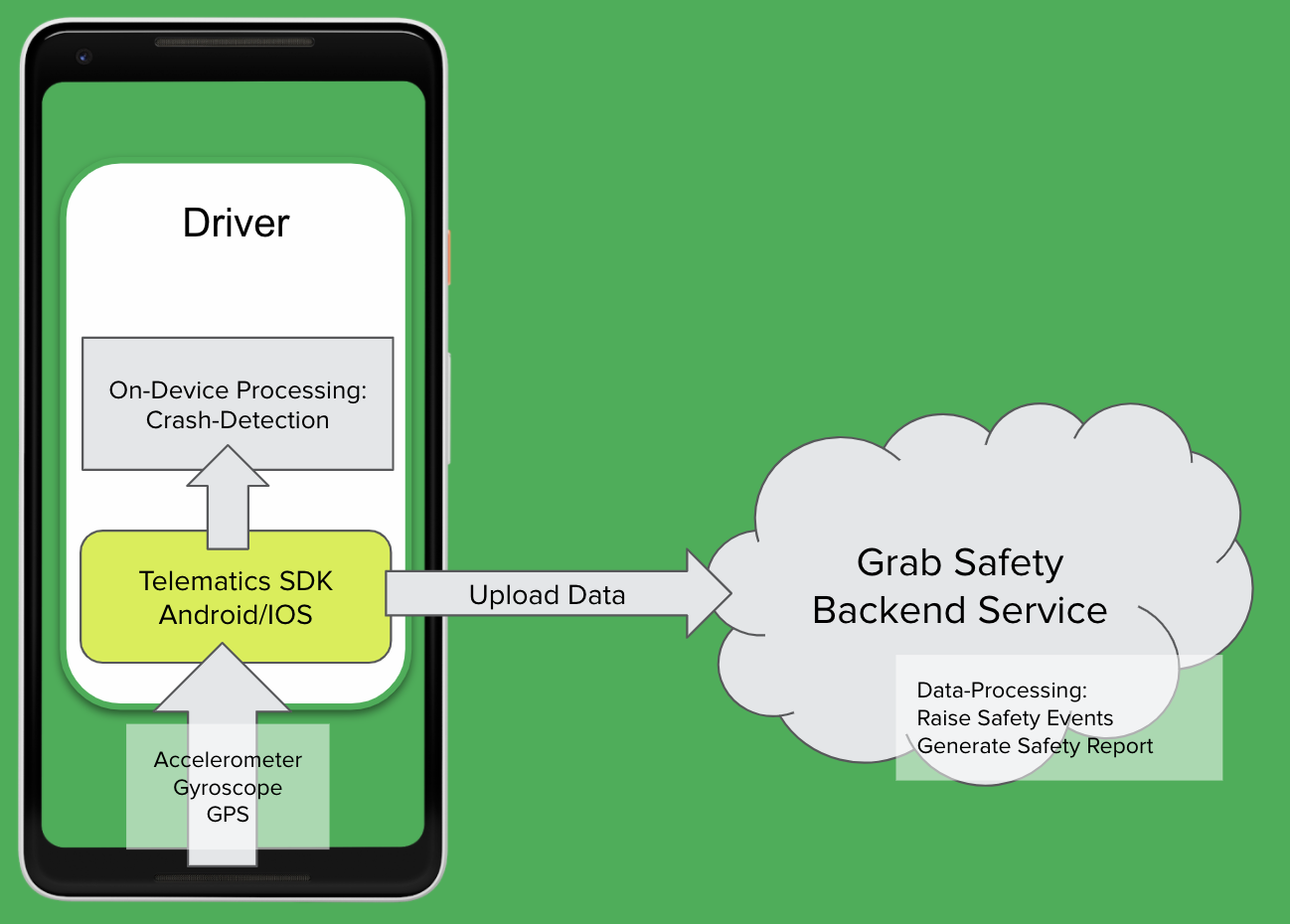
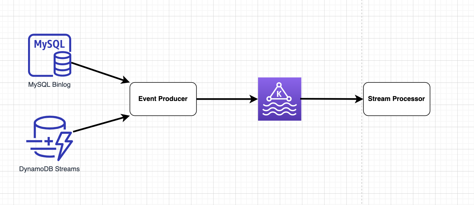
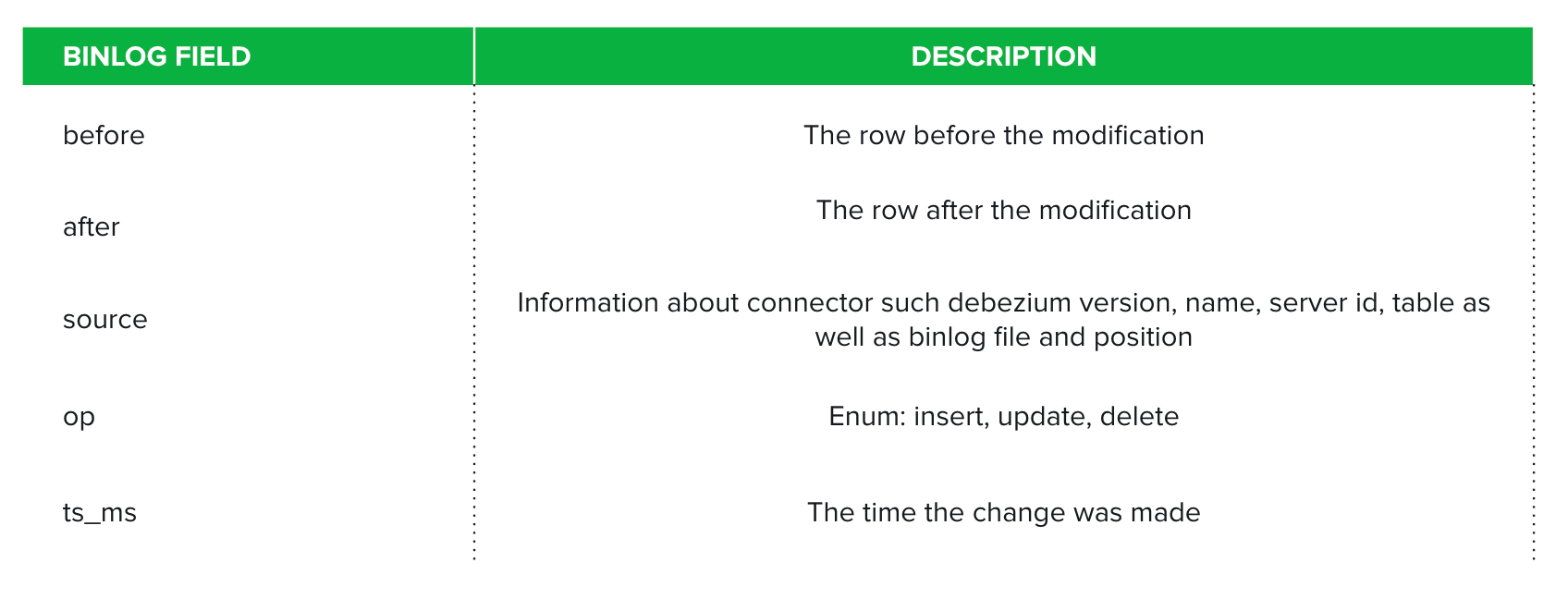
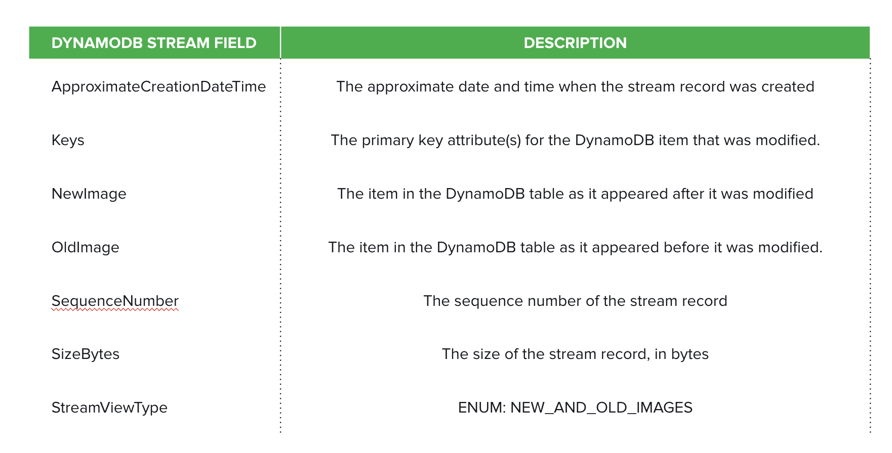
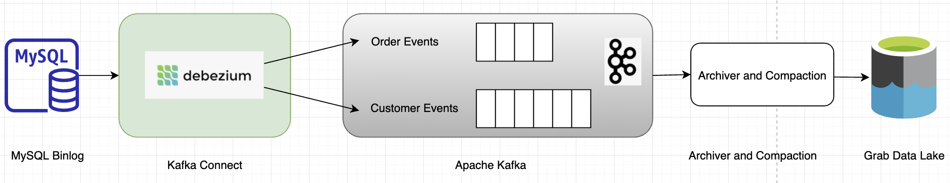
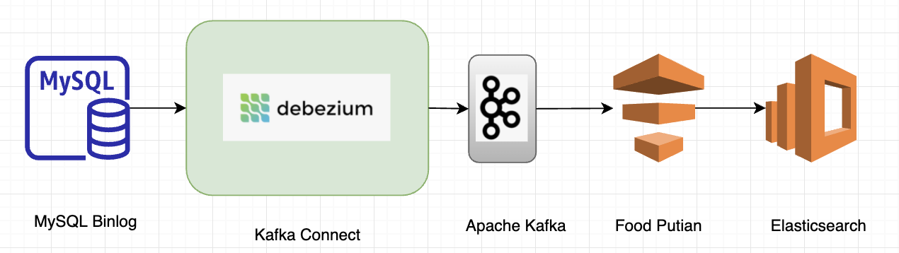
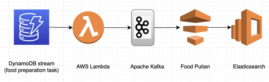
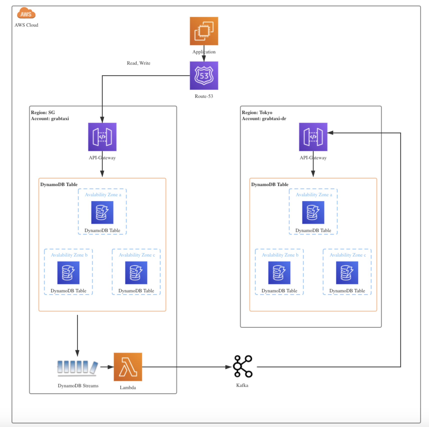
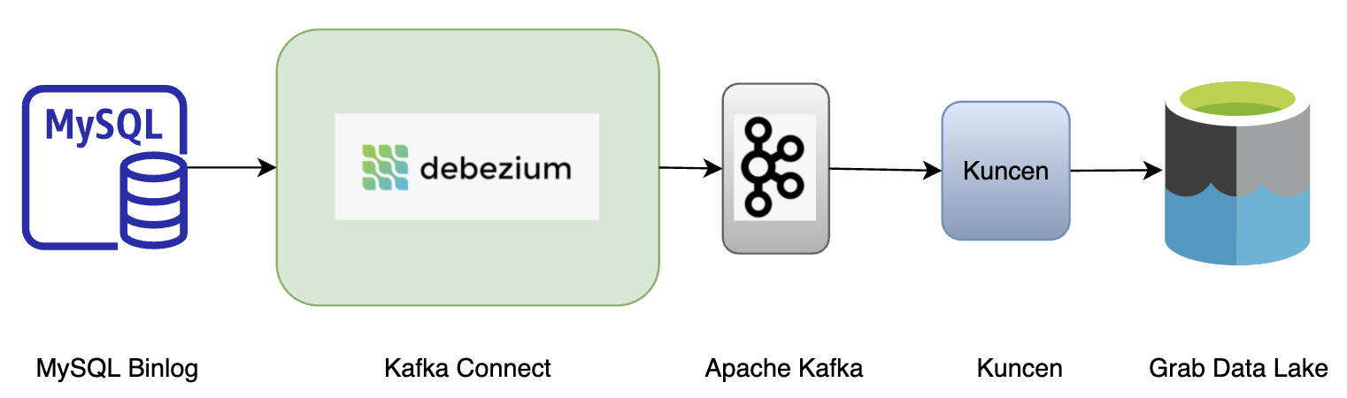

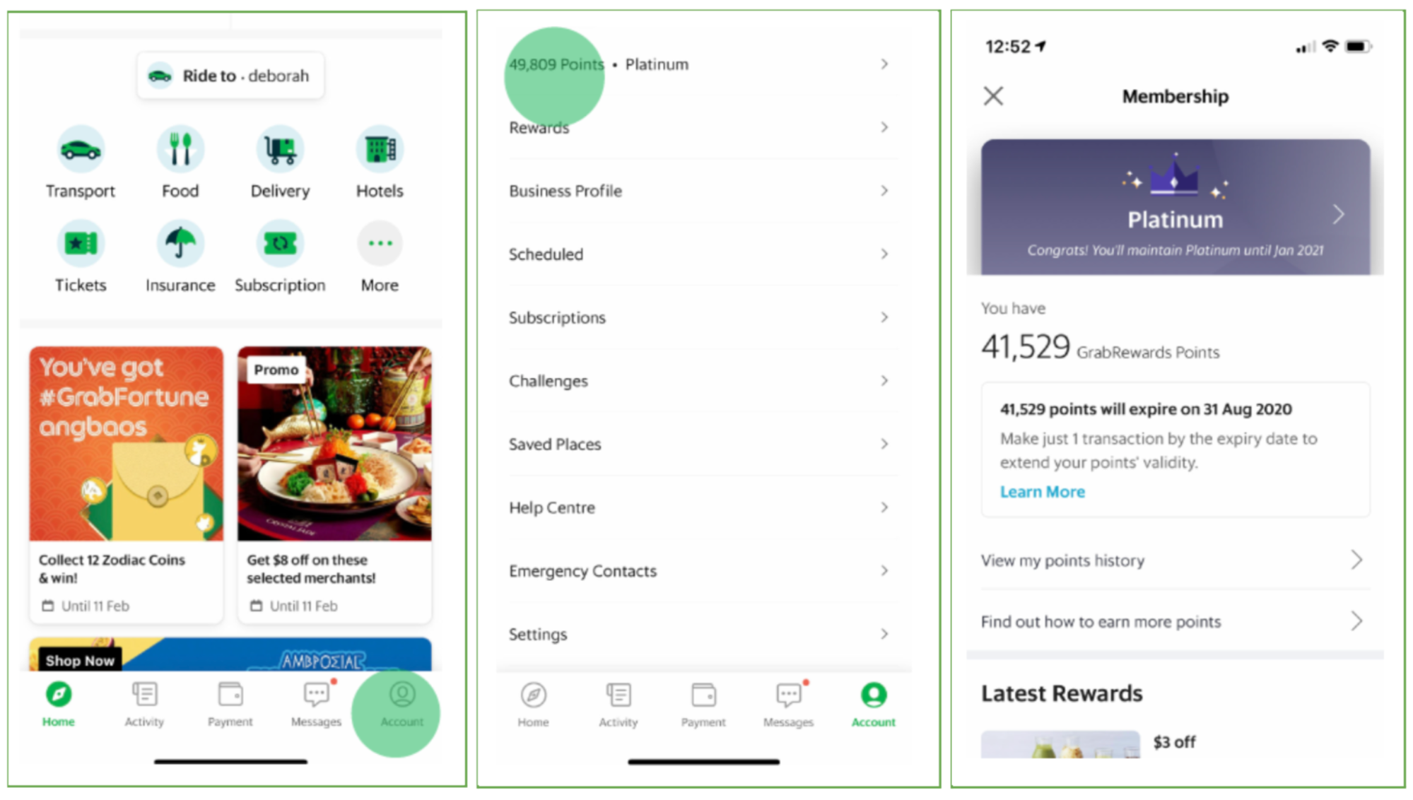
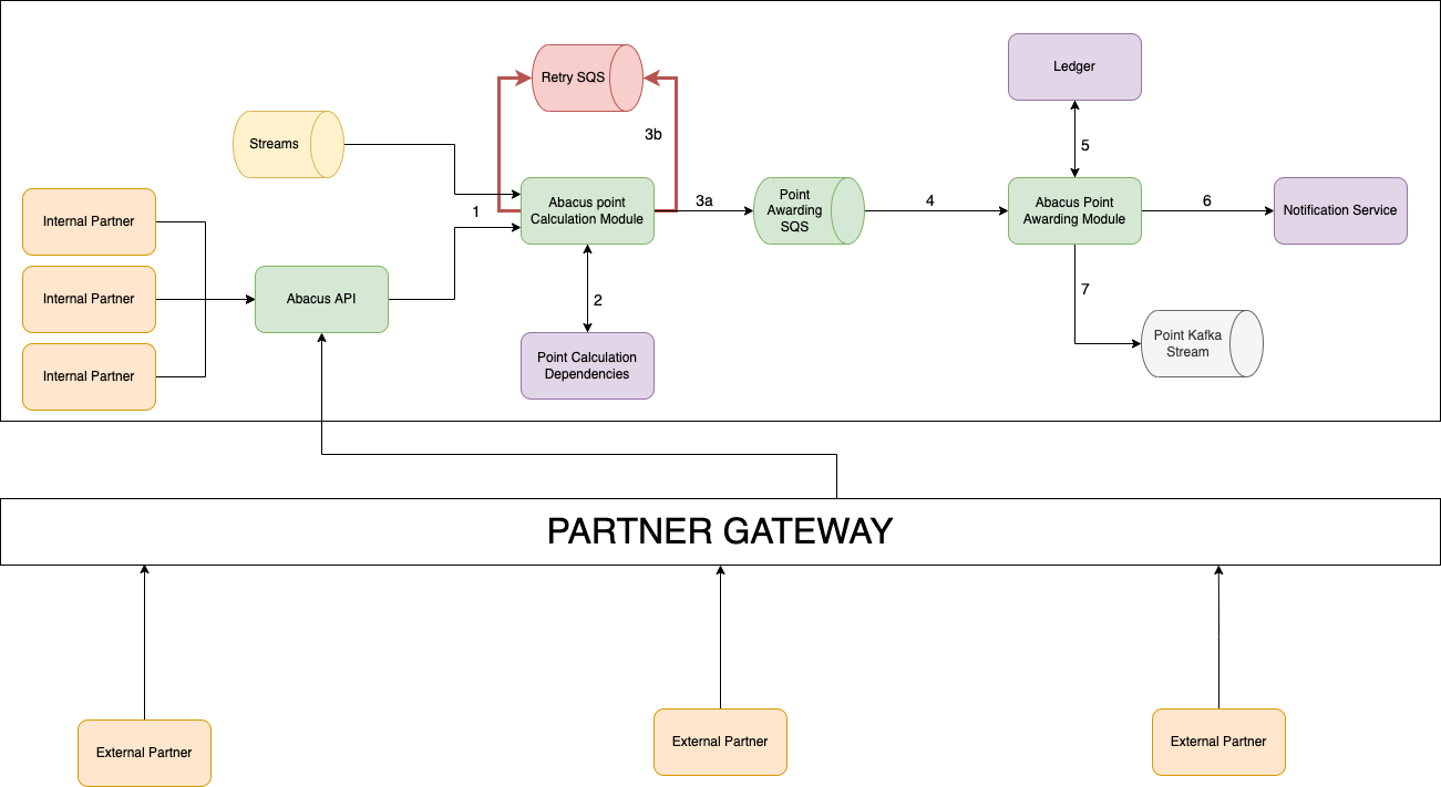
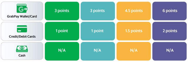
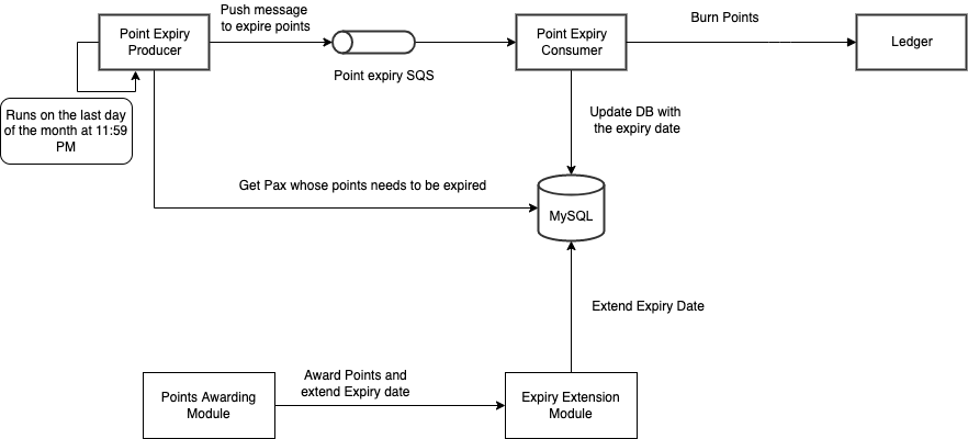

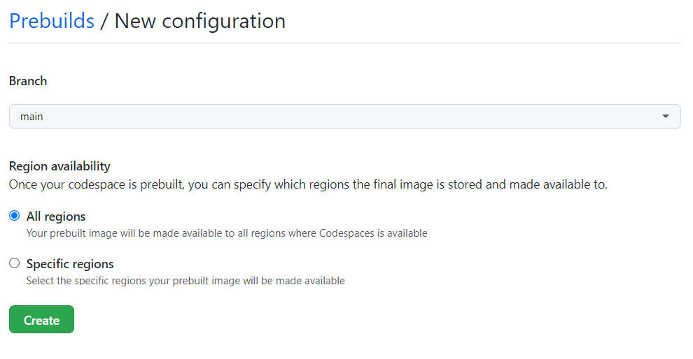
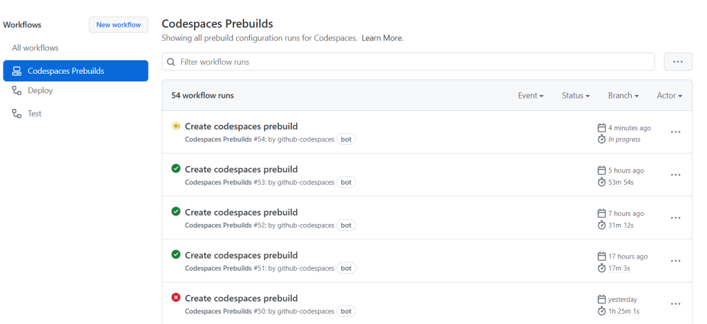
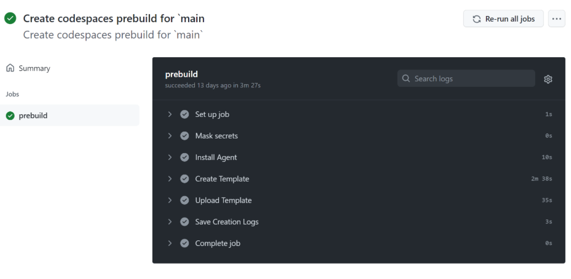
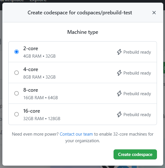
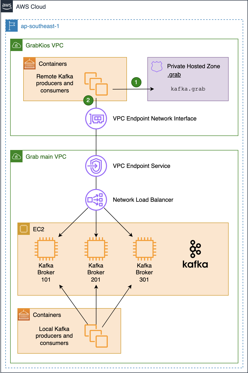
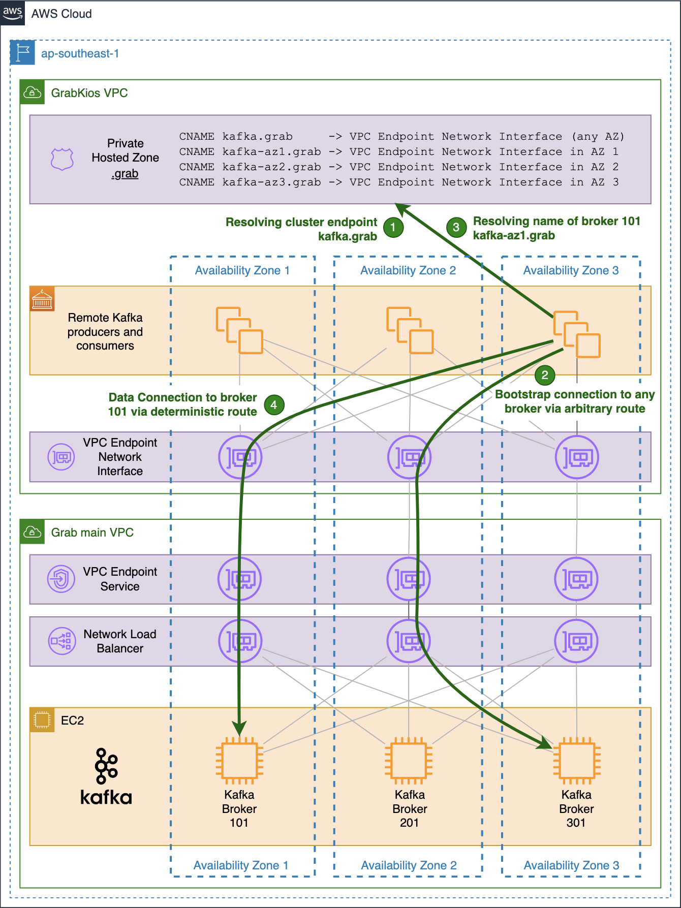
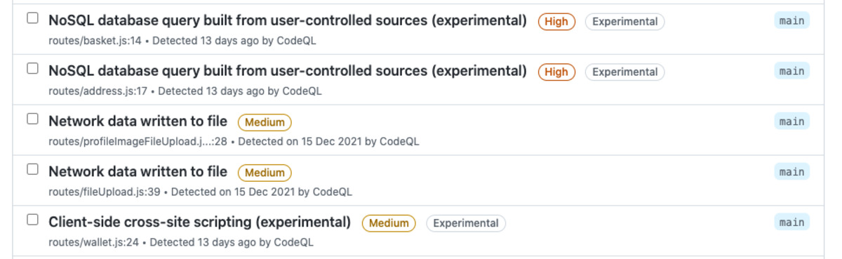
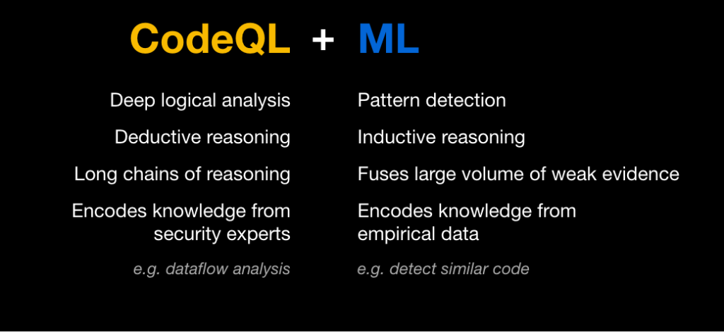


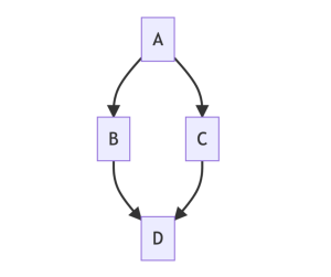
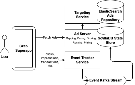
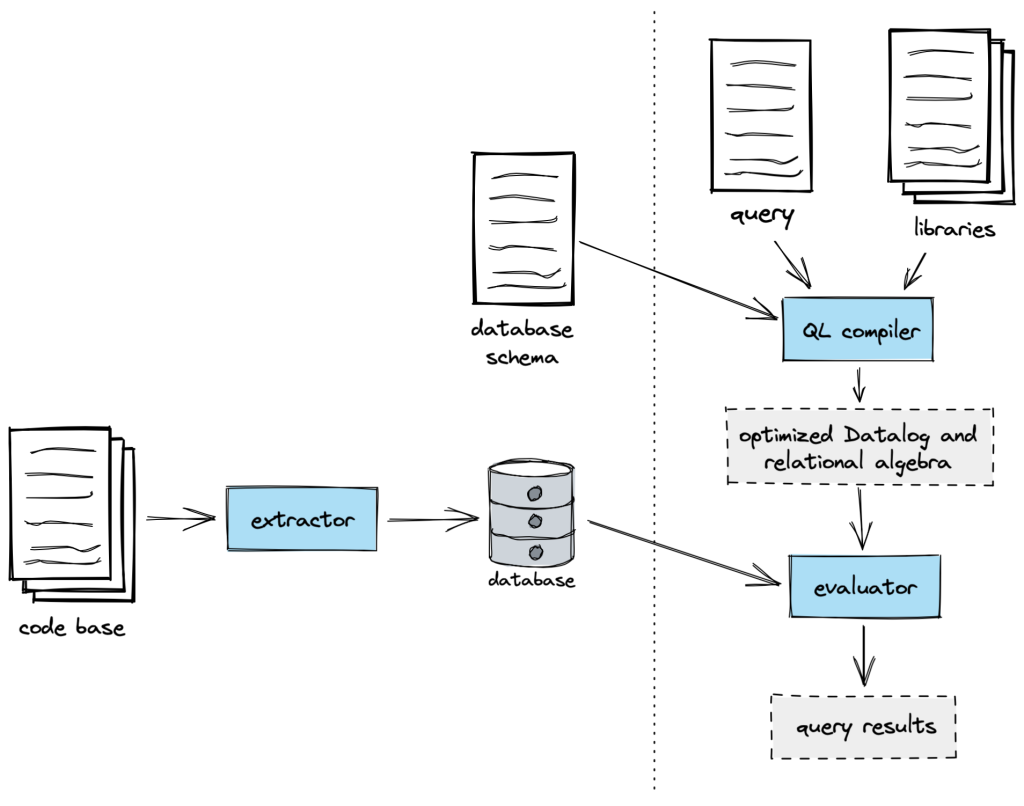
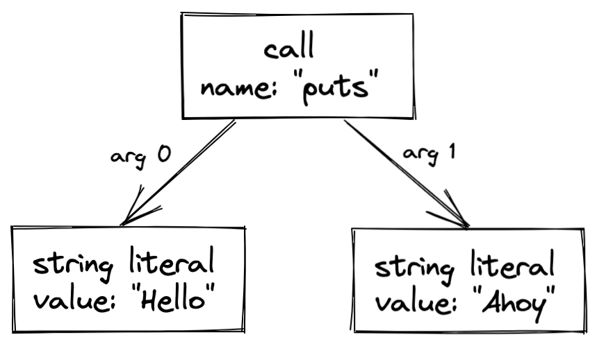

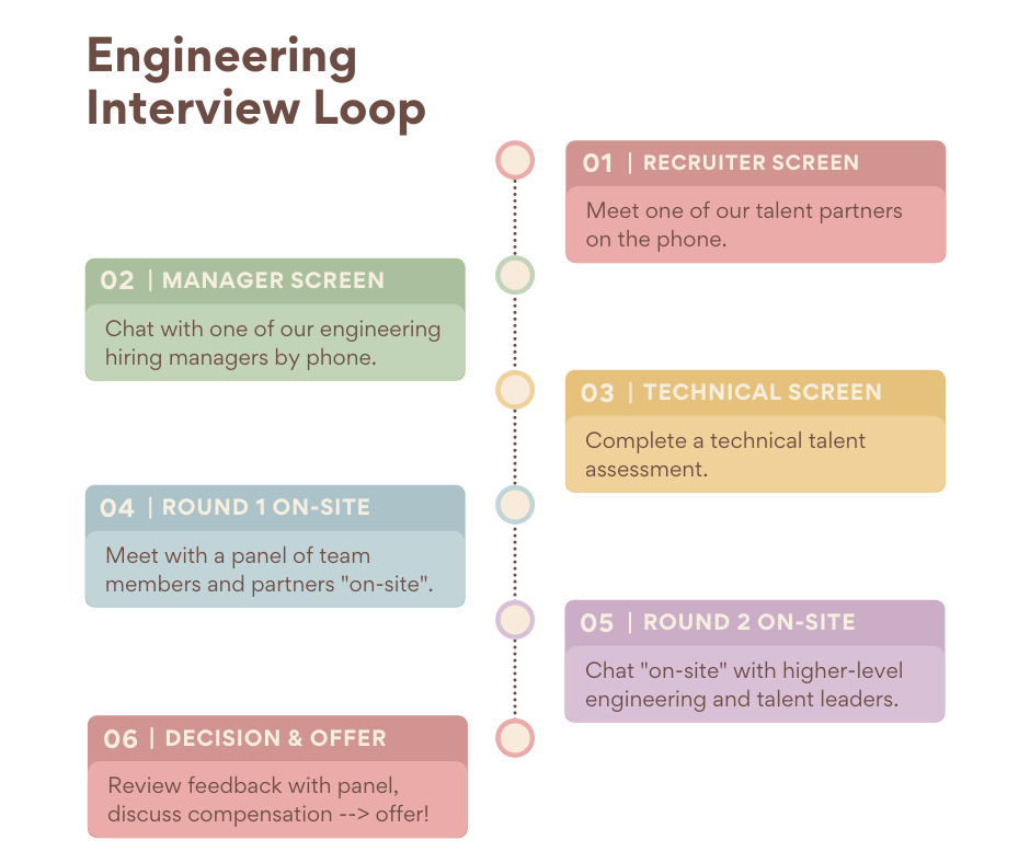


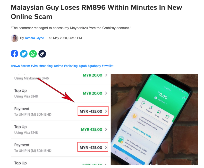
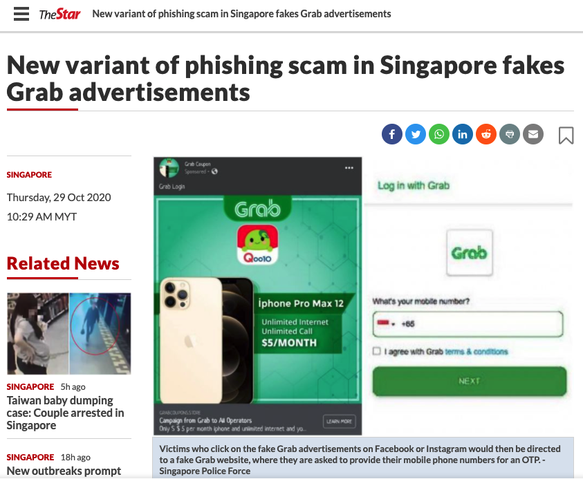
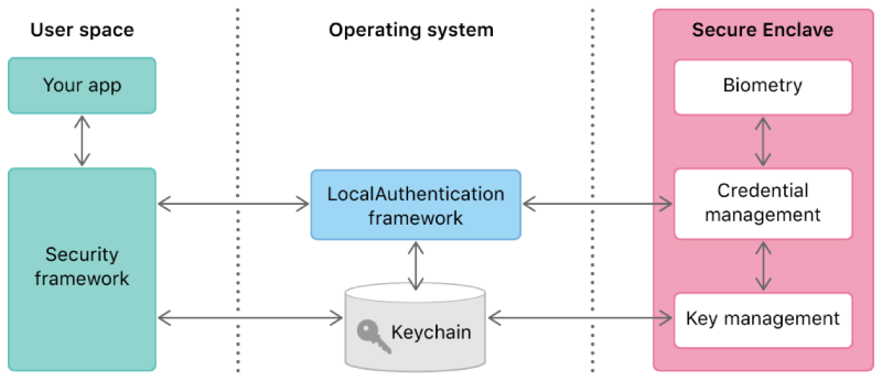
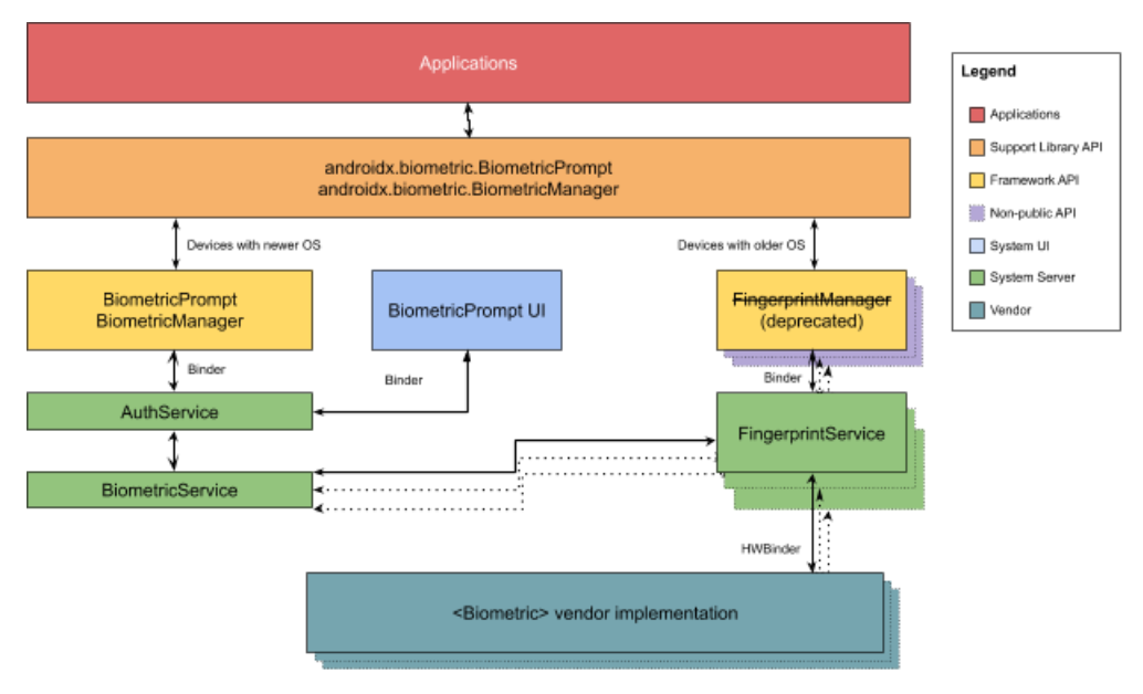
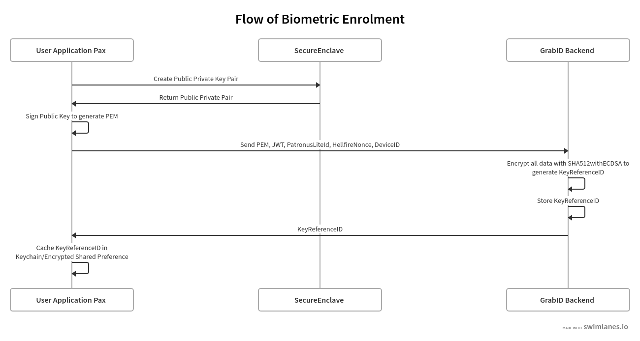


 Conclusion
 ) need not abandon their precious