In April, we experienced three distinct incidents resulting in significant impact and degraded state of availability for Codespaces and GitHub Packages.
April 01 7:07 UTC (lasting 5 hours and 32 minutes)
Our alerting detected an increase in failures to create new Codespaces and start existing stopped Codespaces in the US West region. We immediately updated the GitHub status page and began to investigate.
Upon further investigation, we determined that some secrets that are used by the Codespaces service had expired. Codespaces maintains warm pools of resources to protect our users from intermittent failures in our dependent services. However, in the US West region, those pools were empty of resources due to the expired secret. In this case, we didn’t have an early enough warning on pools reaching low thresholds and didn’t have time to react until we ran out of capacity. As we worked to mitigate the incident, the pools in other regions also emptied due to the expired secret, and those regions began to see failures as well.
A limited number of GitHub engineers had access to rotate the secret, and communication issues delayed the start of the secret refresh process. The expired secret was eventually refreshed and rolled out to all regions, and the service was returned to full operation.
To prevent this failure pattern in the future, we now verify resources that expire and have monitors in place that alert well in advance if pool resources are not being maintained. We’ve also added monitors to notify us earlier when we approach resource exhaustion limits. In addition, we’ve initiated migrating the service to use a mechanism that doesn’t rely on secrets or the need to rotate credentials.
April 14 20:35 UTC (lasting 4 hours and 53 minutes)
We are still investigating the contributing factors and will provide a more detailed update in the May Availability Report, which will be published the first Wednesday of June. We will also share more about our efforts to minimize the impact of future incidents.
April 25 8:59 UTC (lasting 5 hours and 8 minutes)
During this incident, our alerting systems detected increased CPU utilization on one of the GitHub Packages Registry databases, which started approximately one hour before any customer impact occurred. The threshold for this alert was relatively low, and it was not a paging alert, so we did not immediately investigate. CPU continued to rise on the database causing the Package Registry to start responding to requests with internal server errors, eventually causing customer impact. This increased activity was due to a high volume of the “Create Manifest” command used in an unexpected manner.
The throttling criteria configured at the database level wasn’t enough to limit the above command, and this caused an outage for anyone using the GitHub Packages Registry. Users were unable to push or pull packages, as well as being unable to access the packages UI or the repository landing page.
After investigating, we determined there was a performance bug related to the high volume of “Create Manifest” commands. In order to limit impact and restore normal operation, we blocked the activity causing this problem. We are actively following up on this issue by improving the rate limiting in packages and fixing the performance problem that was uncovered. We’ve also modified database alerting thresholds and severity so we get alerted to unexpected issues more quickly (rather than after customer impact).
During this incident, we also discovered that the repository home page has a hard dependency on the packages infrastructure. When the package registry is down, the home pages for repositories that list packages also fail to load. We decoupled the package listing from the repository home page, but that required manual intervention during the outage. We are working on a fix that loosely binds the packages listing, so if it fails, it does not take down the repository home pages for repositories that list packages.
In summary
We will continue to keep you updated on the progress and investments we’re making to ensure the reliability of our services. Please follow our status page for real-time updates. To learn more about what we’re working on, check out the GitHub Engineering Blog.
The Docs-as-Code concept has been gaining traction in the past few years as more tech companies start implementing this approach. One of the most widely-known examples is Spotify, that uses Docs-as-Code to publish documentation in an internal developer portal.
Since the start of 2021, Grab has also adopted a Docs-as-Code approach to improve our technical documentation. Before we talk about how this is done at Grab, let’s explain what this concept really means.
What is Docs-as-Code?
Docs-as-Code is a mindset of creating and maintaining technical documentation. The goal is to empower engineers to write technical documentation frequently and keep it up to date by integrating with their tools and processes.
This means that technical documentation is placed in the same repository as the code, making it easier for engineers to write and update. Next, we’ll go through the motivations behind this initiative.
Why embark on this journey?
After speaking to Grab engineers, we found that some of their biggest challenges are around finding and writing documentation. Like many other companies on the same journey, Grab is rather big and our engineers are split into many different teams. Within each team, technical documentation can be stored on different platforms and in different formats, e.g. Google drive documents, text files, etc. This makes it hard to find relevant information, especially if you are trying to find another team’s documentation.
On top of that, we realised that the documentation process is disconnected from an engineer’s everyday activities, making technical documentation an awkward afterthought. This means that even if people could find the information, there was a good chance that it would not be up to date.
To address these issues, we need a centralised platform, a single source of truth, so that people can find and discover technical documentation easily. But first, we need to change how we write technical documentation. This is where Docs-as-Code comes in.
How does Docs-as-Code solve the problem?
With Docs-as-Code, technical documentation is:
Written in plaintext.
Editable in a code editor.
Stored in the same repository as the source code so it’s easier to update docs whenever a code change is committed.
Published on a central platform.
The idea is to consolidate all technical documentation on a central platform, making it easier to discover and find content by using an easy-to-navigate information architecture and targeted search.
How is Grab embracing Docs-as-Code?
We’ve developed an internal developer portal that simplifies the process of writing, reviewing and publishing technical documentation.
Here’s a brief overview of the process:
Create a dedicated docs folder in a Git repository.
Push Markdown files into the docs folder.
Configure the developer portal to publish docs from the respective code repository.
The latest version of the documentation will automatically be built and published in the developer portal.
Simplified documentation process
This way, technical documentation is closer to the source code and integrated into the code development process. Writing and updating technical documentation becomes part of writing code, and this encourages engineers to keep documentation updated.
Measuring success
Whenever there’s a change throughout big organisations like Grab, it can be tough to implement. But thankfully, our engineers recognised the importance of improving documentation and making it easier to maintain or update.
We surveyed our users and here’s what some have said about our Docs-as-Code initiative:
“[W]ith the doc and source code in one place, test backend engineers can now make doc changes via standard code review process and re-use the same content for CLI helper message and documentation.” – Kang Yaw Ong, Test Automation – Engineering Manager
“[Docs-as-Code] is a great initiative, as it keeps documentation in line and up-to-date with the development of a project. Managing documentation using a version control system and the same tools to handle merges and conflicts reduces overhead and friction in an engineer’s workflow.” – Eugene Chiang, Foundations – Engineering Manager
Progress and future optimisations
Since we first started the Docs-as-Code initiative in Grab, we’ve made a lot of progress in terms of adoption – approximately 80% of Grab services will have their technical documentation on the internal portal by April 2022.
We’ve also improved overall user experience by enhancing stability and performance, improving navigation and content formatting, and enabling feedback. But it doesn’t stop there; we are continuously improving the internal portal and providing more features for our engineers.
Apart from technical documentation, we are also applying the Docs-as-Code approach to our technical training content. This means moving both self-paced and workshop training content to a centralised repository and providing engineers a single platform for all their learning needs.
Special thanks to the Tech Learning – Documentation team for their contributions to this blog post.
We are hiring!
We are looking for more technical content developers to join the team. If you’re keen on joining our Docs-as-Code journey and improving developer experience, check out our open listings in Singapore and Malaysia.
Join us in driving this initiative forward and making documentation more approachable for everyone!
Join us
Grab is the leading superapp platform in Southeast Asia, providing everyday services that matter to consumers. More than just a ride-hailing and food delivery app, Grab offers a wide range of on-demand services in the region, including mobility, food, package and grocery delivery services, mobile payments, and financial services across 428 cities in eight countries.
Powered by technology and driven by heart, our mission is to drive Southeast Asia forward by creating economic empowerment for everyone. If this mission speaks to you, join our team today!
This is the second and final post in a series describing friendly forks and alternative strategies for managing them. Make sure to check out Being friendly: friendly forks 101 for general information on friendly forks and background on the three forks on which we center this post’s discussion.
In the first post in this series, we discussed what friendly forks are and learned about three GitHub-managed friendly forks of git/git, git-for-windows/git, microsoft/git, and github/git. In this post, we deep dive into the management strategies we employ for each of these forks and provide scenarios to help you select the appropriate management strategy for your own friendly fork.
The importance of friendly fork management
While the basics of friendly forks could make for mildly interesting cocktail party conversation , it takes a deeper understanding to successfully manage a fork once you have it. Management (or lack thereof) can make or break friendly forks for the following reasons:
Contributions taken by the upstream project are also generally valuable to the fork.
The number of changes to the upstream project since the last merge is correlated with the difficulty of merging those changes into the fork.
When security patches are pushed upstream, it is critical to be able to easily apply them (without other conflicts getting in the way).
Although there is no one-size-fits-all approach to friendly fork management, our goal for the remainder of this post is to provide a solid starting point for your management journey that will help your friendly fork remain securely in the friend zone.
Our management strategies
We employ a different management strategy for each of the forks discussed in the previous post based on that fork’s unique needs. These strategies are illustrated in the graphic below.
If the above image makes you feel slightly dizzy, don’t worry! We know it’s a lot, so we’re going to break it down into detailed descriptions of how each fork works. Take a deep breath, and prepare to dive in.
git-for-windows/git
Git for Windows uses a custom merging rebase strategy to take changes from upstream. A merging rebase is just what it sounds like-a combination of a merge and a rebase. Merging rebases are executed at a predictable cadence that follows the git/git release cycle.
When it is time for a new release, git/git creates a series of release candidate tags (typically rc0, rc1, rc2, and final) on its default branch. As soon as each new candidate is released, we execute a merging rebase of the main branch on top of it. The merge portion comes first, with this command:
$ git merge -s ours -m "Start the merging-rebase to <version>" HEAD@{1}
This creates what we call a “fake merge” since it uses the “ours” strategy to discard all the changes from main. While this may seem odd, it actually provides the benefits of a clean slate for rebasing and the ability to fast forward from previous states of the branch.
After the merge is complete, the rebase commences. This portion of the process helps us resolve merge conflicts that occur when upstream changes conflict with changes that have been made in git-for-windows/git. One type of conflict in particular is worth discussing in more depth: commits that have been added to git-for-windows/git and subsequently upstreamed.
When these commits are submitted upstream, the community supporting git/git usually requests changes before they are accepted. Additionally, since git/git only accepts patches sent via mailing list (instead of pull requests), commit IDs inevitably change when applied upstream. This means there will be conflicts when git-for-windows/git is rebased on top of a new release. Running the following command helps us identify commits that have been upstreamed when we encounter conflicts:
This command compares the differences between the below ranges of commits, dropping any that are not in the first specified range:
From the commit before the commit you are checking to the commit you are checking (this will only contain the commit you are checking).
The upstream commits that are not in the commit history of <commit>.
If there is a matching commit in upstream, it will be shown in the command’s output. In this case, we use git rebase --skip to bypass the commit (and implicitly accept the upstream version).
Because git-for-windows/git begins its merging rebase immediately after the creation of each release candidate, we classify it as proactive-it ensures all new git/git features are integrated and released as soon as possible. The merging rebase is generally executed for each release candidate by one developer, but is reviewed by multiple other developers with the help of range-diff comparisons. You can find an example of such a review here. When complete, the changes are pushed directly to the main branch, and a new release is created.
microsoft/git
Like git-for-windows/git, microsoft/git is proactive, executing rebases immediately following the creation of each new git/git release candidate. It also uses the same strategies for identifying commits that have made it upstream. However, there are a few key differences between the git-for-windows/git approach and the microsoft/git approach. These are:
Since microsoft/git is a fork of git-for-windows/git, it does not take commits directly from git/git. Instead, we wait for the git-for-windows/git merging rebase to complete for each candidate then rebase on top of the resulting tag.
Instead of repeatedly rebasing a designated main branch, we cut a brand new branch for each version with the naming scheme vfs-2.X.Y (see the current default as an example). This branch is based off the initial git-for-windows/git release candidate tag and is updated with the rebase for each new release candidate. We based this strategy on release branches in Azure DevOps to make hotfixing easier and to clarify which commits are released with each new version.
Once the rebases are complete, we designate vfs-2.X.Y, as the new default branch, and create a new release.
github/git
github/git integrates new git/git releases using a traditional merge strategy. It is cautious in its cadence for taking releases; for this fork, we prefer to allow new features to “simmer” for some time before integration. This means that github/git is typically one or two versions behind the latest release of git/git.
To ensure merges are high-quality and accurate, the merge of a new git/git version is carried out by at least two developers in parallel. For commits that began in github/git and subsequently made it upstream, we generally accept the upstream version when resolving resulting conflicts. Occasionally, however, there are reasons to take the github/git version (or, some parts of both versions). It is up to the developers executing the merge to decide the correct strategy for a particular commit. When each merge is complete, the trees at the tip of each merge are compared, and the different approaches to conflict resolution are reviewed. The outcome of this review is merged and deployed as a new release.
Note that there are tradeoffs to the decision to use a traditional merge strategy to manage this fork. Merging is more straightforward than rebasing or rebase merging. However, merges in github/git can become somewhat tricky when it has drifted far from upstream or when a sweeping change in upstream affects many parts of its custom code. Additionally, this strategy requires all commits to be preserved (as opposed to git-for-windows/git and microsoft/git, which use the autosquash feature of the rebase command to remove squash and fixup commits), which means more commits are involved in github/git merges.
Comparison
Below is a side-by-side summary of the key similarities and differences in the management strategies discussed above.
Fork
Management Strategy
# of developers executing
Proactive or cautious
Long-running main branch
Integrates release candidates
git-for-windows/git
merging rebase
1
Proactive
Yes
Yes
microsoft/git
merging rebase
1
Proactive
No
Yes
github/git
merge
>=2
Cautious
Yes
No
As shown in the table, git-for-windows/git and microsoft/git have a lot in common. They are both proactive, executed by one developer, and use a form of rebase to integrate new releases (and release candidates). github/git is a bit different in its choice of a merge management strategy, the number of developers that simultaneously execute this strategy, and its cautious approach to integrating new releases (and in that release candidates are not considered).
As lovely as the above table is, you may still be scratching your head, wondering which strategy is right for you or your organization. Never fear! Our final section provides a series of scenarios with the goal of making this decision easier for you.
Finding your perfect match
Well done! You’ve successfully made it through our deep dive into three alternatives for friendly fork management.
However, now comes the really important part! It’s time to take a good look at each of the above strategies to understand which one is the best fit for you. We’ve organized this section as a series of scenarios to help you frame the above in the context of your own needs. Keep reading if you’re ready to choose your own friendly fork adventure!
Scenario 1: You have many contributors working simultaneously.
Constantly creating new default branches can leave developers with open pull requests in a bad state; obviously, this is particularly problematic when there’s a healthy amount of active development in your repository. Consider a merge or merging rebase strategy to avoid changing default branches and requiring your developers to constantly rebase.
Scenario 2: You need to support multiple versions with security releases or other bug fixes.
Consider the rebase model to have an easy story for cherry-picking fixes to supported versions.
Note: it is also possible to cherry-pick features from upstream with a merge-based workflow. However, if you later merge the commits containing the cherry-picked features, you may have to resolve some trivial conflicts depending on your merge strategy.
Scenario 3: You don’t (or do!) want to take new features immediately.
You can apply a cautious or proactive approach to any of the above strategies. Work with your team/management to find a cadence everyone is comfortable with and stick to it.
Scenario 4: You’re new to the fork game and want to keep it simple.
If this is your (or, your team’s) first time managing a fork and/or you’re just learning your way around Git, the merge strategy may be the most straightforward place for you to start.
Still not sure which strategy to use? Consider getting in touch with the maintainers of one of the friendly forks listed above (for example, via the appropriate mailing list(s) or a GitHub discussion) to get input from the experts!
Wrapping up
A friendly fork can help accelerate development and increase developer productivity and satisfaction. Additionally, managing a friendly fork carefully to stay in the friend zone can lead to successful collaboration between different communities and improved project quality for all parties involved. We hope this series has helped you understand whether a friendly fork is right for you or your organization and, if so, empowered you to create and begin managing your friendly fork successfully.
We’re proud to announce the availability of search-based code navigation for the Elixir programming language. Yet this is more than just new functionality. It’s the first example of a language community writing and submitting their own code for search-based code navigation.
Since GitHub introduced code navigation, we’ve received enthusiastic feedback from users. However, we hear one question over and over again: “When will my favorite language be supported?” We believe that every programming language deserves best-in-class support in GitHub. However, GitHub hosts code written in thousands of different programming languages, and we at GitHub can commit to supporting only a small subset of these languages ourselves. To this end, we’ve been working hard to empower language communities to integrate with our code navigation systems. After all, nobody understands a programming language better than the people who build it!
Community contributions welcome!
Would you like to develop and contribute search-based code navigation for a language? If a Tree-sitter grammar tool exists for your language, you can do so using Tree-sitter’s tree query language. This language describes how our code navigation systems scan through syntax trees and how to extract the important parts of a declaration or reference. This process is known as tagging, and it’s integrated with the tree-sitter command-line tool so that you can run and test tag queries locally. When a user pushes new commits or creates a pull request, the GitHub code navigation systems use tag queries to extract jump-to-definition and find-all-references information. Note: If you’re interested in how search-based code navigation works, you can read a technical report that describes the architecture and evolution of GitHub’s implementation of code navigation.
How do I get started?
Complete documentation, including how to write unit tests for your tags queries, can be found here. For examples of tag queries, you can check out the Elixir tags implementation, or those written for Python or Ruby. Once you’ve implemented tag queries for a language, have written unit tests, and are satisfied with the output from tree-sitter tags, you can submit a request on the Code Search and Navigation Feedback discussion page in the GitHub Discussions page in the GitHub feedback repository. The Code Navigation team will add this to their roadmap. When we’re confident in the quality of yielded tags and the load on the back-end systems that handle code navigation, we can enable it in testing for a subset of contributors, eventually rolling it out to all GitHub users, on both private and public repositories.
Please note that search-based code navigation is distinct from GitHub code search. Code search provides a view across all of the corpus of code on GitHub, whereas search-based code navigation is a part of the experience of reading code within a single repository. Search-based code navigation is also distinct from our support for precise code navigation. However, we hope to empower language communities to inform and contribute to the development of and support for these and other features in the future.
We’re committed to working with language maintainers and contributors to keep these rules as useful and up-to-date as possible. Whether you’re a longtime language contributor or someone seeking to enter the community for the first time, we encourage you to take a look at adding support for search-based code navigation, and join the community on the GiHub Discussions Page.
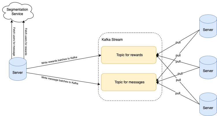
As a leading superapp in Southeast Asia, Grab serves millions of consumers daily. This naturally makes us a target for fraudsters and to enhance our defences, the Integrity team at Grab has launched several hyper-scaled services, such as the Griffin real-time rule engine and Advanced Feature Engineering. These systems enable data scientists and risk analysts to develop real-time scoring, and take fraudsters out of our ecosystems.
Apart from individual fraudsters, we have also observed the fast evolution of the dark side over time. We have had to evolve our defences to deal with professional syndicates that use advanced equipment such as device farms and GPS spoofing apps to perform fraud at scale. These professional fraudsters are able to camouflage themselves as normal users, making it significantly harder to identify them with rule-based detection.
Since 2020, Grab’s Integrity team has been advancing fraud detection with more sophisticated techniques and experimenting with a range of graph network technologies such as graph visualisations, graph neural networks and graph analytics. We’ve seen a lot of progress in this journey and will be sharing some key learnings that might help other teams who are facing similar issues.
What are Graph-based Prediction Platforms?
“You can fool some of the people all of the time, and all of the people some of the time, but you cannot fool all of the people all of the time.” – Abraham Lincoln
A Graph-based Prediction Platform connects multiple entities through one or more common features. When such entities are viewed as a macro graph network, we uncover new patterns that are otherwise unseen to the naked eye. For example, when investigating if two users are sharing IP addresses or devices, we might not be able to tell if they are fraudulent or just family members sharing a device.
However, if we use a graph system and look at all users sharing this device or IP address, it could show us if these two users are part of a much larger syndicate network in a device farming operation. In operations like these, we may see up to hundreds of other fake accounts that were specifically created for promo and payment fraud. With graphs, we can identify fraudulent activity more easily.
Grab’s Graph-based Prediction Platform
Leveraging the power of graphs, the team has primarily built two types of systems:
Graph Database Platform: An ultra-scalable storage system with over one billion nodes that powers:
Graph Visualisation: Risk specialists and data analysts can review user connections real-time and are able to quickly capture new fraud patterns with over 10 dimensions of features (see Fig 1).
Fig 1: Graph visualisation
Network-based feature system: A configurable system for engineers to adjust machine learning features based on network connectivity, e.g. number of hops between two users, numbers of shared devices between two IP addresses.
Graph-based Machine Learning: Unlike traditional fraud detection models, Graph Neural Networks (GNN) are able to utilise the structural correlations on the graph and act as a sustainable foundation to combat many different kinds of fraud. The data science team has built large-scale GNN models for scenarios like anti-money laundering and fraud detection.
Fig 2 shows a Money Laundering Network where hundreds of accounts coordinate the placement of funds, layering the illicit monies through a complex web of transactions making funds hard to trace, and consolidate funds into spending accounts.
Fig 2: Money Laundering Network
What’s next?
In the next article of our Graph Network blog series, we will dive deeper into how we develop the graph infrastructure and database using AWS Neptune. Stay tuned for the next part.
Join us
Grab is the leading superapp platform in Southeast Asia, providing everyday services that matter to consumers. More than just a ride-hailing and food delivery app, Grab offers a wide range of on-demand services in the region, including mobility, food, package and grocery delivery services, mobile payments, and financial services across 428 cities in eight countries.
Powered by technology and driven by heart, our mission is to drive Southeast Asia forward by creating economic empowerment for everyone. If this mission speaks to you, join our team today!
This is the first post in a two-part series describing friendly forks and alternative strategies for managing them. Stay tuned for part two coming in May!
This post covers what a friendly fork is, why they are beneficial, and how they differ from a divergent fork. We’ll also look at some examples from the wild and provide details on three of our favorite friendly forks of the git/git repository.
To fork or not to fork
Most developers are familiar with the concept of working with source code in repositories. However, what should you do when you want to make one or more major changes to a repository that you do not own? Two options are to submit feature requests or to contribute the features you need yourself. This is a very common approach in open source software, and, when it goes well, it can lead to productive collaboration and useful results for all parties.
But what if the proposed features are not accepted into the repository? What if they were never intended to be contributed back to the original project? If you (or your company) have a strong need for these features, creating a friendly fork of the repository could be the right choice.
What is a friendly fork?
A friendly fork is a long-lived fork that complements its upstream repository (i.e., the repository from which it was forked) with customizations targeted to a subset of users. Typically, features from the friendly fork are contributed back to the upstream repository through a process known as upstreaming. If that is the case, developers working in the friendly fork sustain relationships with the maintainers of the upstream repository (this is the friend zone we’re so fond of!) to facilitate this flow of features and to improve the software for both user bases. It is also possible, however, for a friendly fork to simply take regular updates from its upstream repository with no maintainer interaction. Friendly forks may or may not eventually re-merge with the upstream repository.
Below are some examples of existing friendly forks of the git/git repository (which are maintained by folks at GitHub) and their purposes.
git-for-windows/git: hosts Windows-specific features of Git. It also sometimes receives early features which are subsequently upstreamed into git/git.
microsoft/git: focuses on features to support monorepos, some of which are subsequently upstreamed into git/git.
github/git: powers GitHub’s backend. It includes GitHub-specific changes, like extra instrumentation specific to GitHub’s infrastructure, but also serves as a staging ground for new features before they are submitted upstream.
git/git is definitely not the only repository with friendly forks. Examples of friendly forks created from other repos include:
MSYS2: a fork of Cygwin that provides an environment for building, installing, and running native Windows software.
CentOS: a fork of Red Hat Enterprise Linux (RHEL) created in 2004 to offer a RHEL-like experience for the community. (Interestingly, Red Hat now owns the CentOS trademarks).
It is important to note that not all forks can be considered friendly. There are also divergent forks, which are typically created due to insurmountable disagreements in a community caused by disparate goals or personality conflicts. Divergent forks often become so different from their upstream repositories that sharing code becomes difficult, if not impossible. While it is good to know that divergent forks are a thing you may encounter in the wild, we emphatically believe in the power of the friend zone and will center our focus for the rest of this series on getting and keeping forks there.
A tale of three forks
Three of the friendly fork examples provided above are based off of git/git, git-for-windows/git, microsoft/git, and github/git. Each of these forks has a unique history that contributes to the strategy used to maintain it. We will dedicate the remainder of this post to describing the history and purpose of each fork.
git-for-windows/git
git-for-windows/git is the oldest of our forks for discussion. It was created in 2007 to provide the required adjustments to Git for it to run on Windows. While it may seem odd that Windows-specific features weren’t just added to the git/git repository, forking was deemed necessary because the git/git project was (and, still is) run by experts in the Unix systems domain. And Windows, of course, falls outside the scope of that expertise.
Although this fork was originally intended to be short-lived, it soon became clear that Windows support would be an ongoing community need that would require a permanent fork. Thus, development in git-for-windows/git continues in earnest today.
Because it was created to give Windows users the option of using Git for version control, the main purposes of git-for-windows/git are:
Provide a seamless, pain-free experience for Windows users.
Separation of concerns (in other words, Windows-specific and Unix-specific features are contributed in different repositories, while shared features can easily flow between the repositories).
As with each fork we discuss in this post, there are some use cases for which it makes sense for new features to be contributed to the fork before they are added upstream. FS Monitor is an example of this in which the Request for Comments went to the git/git mailing list, but early implementations of the feature were merged into git-for-windows/git for rapid testing.
microsoft/git
microsoft/git began as a private fork of git-for-windows/git, with the initial purpose of supporting Microsoft-internal products. However, it was open-sourced in 2017, and, as a result, its goals today are much more general and community-oriented:
Facilitate easy dogfooding/quick releases of new features for GitHub’s monorepo customers.
As with git-for-windows/git, determine which of these features make sense to contribute back upstream and submit/monitor them on the mailing list.
An example feature that was introduced to microsoft/git prior to upstreaming is the sparse index. This was done to speedily get this new feature into the hands of monorepo customers who needed it most. After that was done, the feature was gradually introduced and refined upstream.
github/git
github/git, our final fork for discussion, actually did not begin as a fork. In the early days of GitHub, we carried a handful of changes on top of new Git releases. Because there were only a few, we stored them as *.patch files that got applied on top of each new release before deployment. Over time, however, our custom changes became both more numerous and more applicable to being contributed to git/git. It became clear that a full-fledged fork would be beneficial to improve management, workflows, and our ability to contribute back to upstream. Thus, in 2012, the official github/git fork was born.
Note that github/git differs from the above forks in that it is a private friendly fork, while the other two are public. Private friendly forks can be very beneficial to organizations. For example, they can be an excellent testing ground for new features, as they allow you to be confident code has been battle-tested internally and works before submitting publicly upstream. They can also be less beholden to the upstream release cadence, which helps ensure stability for the product.
To this day, this fork serves the same purpose of powering GitHub’s infrastructure. It fulfills our need to support features specialized to this infrastructure and is also used as a “staging ground” for new features before submitting them to the open source git/git repository. Specific examples of the latter use include bitmaps and multi-pack bitmaps.
That’s all for now!
In this post, we’ve discussed what a friendly fork is and how friendly forks differ from divergent forks. We’ve learned about three different friendly forks of the git/git repository and their purposes for existing. Thanks for sticking with us this far, and be sure to keep your peeled for our second post in the “friend zone” series, in which we’ll talk about how these forks are managed and how you can adapt their strategies to your very own friendly fork!
At GitHub, we relentlessly pursue performance. Join me now for the tale of how we dropped a P99 time by 95% on code that runs for every single Git push operation.
Every time you push to GitHub, we run a set of checks to validate your push before accepting it. If you ever tried to push an object larger than 100MB, you are already familiar with them, as these pre-receive hooks contain that logic. Similarly, they do other checks, such as verifying that LFS objects have been successfully uploaded. These hooks help keep our servers healthy and improve the user experience.
We recently rewrote these hooks from their original Ruby implementation into Go. This rewrite was something we had in mind for a while, but what really sold us on the effort was the potential performance improvement.
Today, we’ll talk about the history of these hooks, how we discovered that the performance was problematic, and how we went about safely replacing them.
How did we get here?
We created the first hook in 2013 to warn users that a repository was renamed. The only action was a database check for a previous name and to send a warning to the user to update their remote URL. At the time, almost all of GitHub was part of one Ruby on Rails application, so it was the logical choice for hooks as well. As time passed, more and more functionality was added to the hooks, requiring additional configuration, exception reporting, and logging.
This meant that hooks imported the same dependencies as the Ruby application. Over time, the number of dependencies, and therefore startup time, only increased. In a Rails application, these dependencies are loaded only once at startup time, and then each request has them available, making the startup time not important for the user experience. However, these hooks are run as subprocesses underneath the Git executable, so they are loaded for each request, making the startup time critical to performance. When we investigated, loading these dependencies took a rather long time. Hooks took about 880 milliseconds to execute on average, and almost all of that time was spent loading dependencies. In addition, there are two sets of hooks: one with the new data under quarantine and a second set once the data is available in the repository. Especially with this double execution, this startup time significantly affects each push. An empty push could take more than two seconds, which was unacceptable.
Why rewrite?
Since the performance issues were related to startup time, we had a few options. We could reduce the number of dependencies, we could change the architecture so that hooks only started up once, or we could rewrite the hooks to run independently of the monolith. Rewrites and changing the architecture carry risk, so we tried the simplest alternative first.
Loading fewer dependencies while staying within the Rails monolith proved quite tricky. There were a lot of dependencies (more than 450 gems leading to over 1,000 require calls), and they were all quite tangled up in the app’s configuration, because they were not designed to be used outside of the GitHub Rails monolith. However, careful use of the debugger and strace revealed a few outliers that we could avoid loading when running the hooks. This removal dropped 350-400 milliseconds from the startup time.
While this was already a decent improvement for a small tweak, the startup time was still quite slow, and we weren’t satisfied yet. Additionally, new dependencies are frequently added to the Rails application, which means that the startup time would creep up again over time even if our hook code did not change.
How did we rewrite?
We could not ignore the configuration from the Rails app as that is how we know how to connect to the database, send stats, etc. Some of that could be duplicated at the risk of having two parallel configuration paths that would almost certainly end up diverging.
To pass configuration along that only the app knows about, we were able to use an existing mechanism, which was already in use to pass along information, such as the name of a repository and whether it is over its quota. This comes alongside other information necessary to perform updates so it gets called for every push, and adding some more data there adds very little overhead. We identified the information necessary to perform the checks and added this information.
For the past few years, the Git Systems Team has been extracting more and more of our service code from the Rails monolith and rewriting it as a dedicated service written in Go. Based on this experience with Go, and given what we learned about the Ruby hooks, moving the hooks into this Go service seemed like a natural fit as well. Just extracting the hooks to run independently of the Rails apps would have removed most of the boot time, but Go gives us the last few milliseconds and lets us make them part of the service in which the backend code increasingly lives. We expected such a significant rewrite to be worth the risk, because afterwards the hooks should be much faster.
Further, as we commonly do for high-impact changes, we put these rewritten hooks behind a feature flag. This gave us the ability to enable them for individual repositories or groups of them. We started with a few internal GitHub repositories to confirm the effect in production.
The results were so impressive that we had to double check that the hooks were still running. It was hard to distinguish between really fast hooks and completely disabled hooks. The median time was now 10ms, compared to roughly 880ms when we started the project. This made pushes noticeably faster for everyone. We even got unprompted questions about whether pushing had become faster after someone noticed it on their own.
Lessons learned
This is a project we had in mind for a long time. We had wanted to rewrite these hooks outside of the monolith to separate our area of responsibility better. However, merely having a better architecture often isn’t enough to make something a business priority. By tying the change to its impact on users we could prioritize this work. We came away with the dual benefits of a much better user experience and an architectural improvement.
This change has now been live on github.com for a couple of months, and has been shipped in GHES 3.4, so everyone now saves some time pushing to their GitHub repositories.
Today, we’re releasing exciting improvements that will streamline your Codespaces experience when working with multi-repository projects and monorepos. Codespaces are instant cloud-powered development environments that aim at maximizing your productivity by eliminating set-up times regardless of the type, size, and complexity of your projects.
With our initial release, we wanted to address the most common type of projects hosted on GitHub: cloud-native applications housed in a singular repository. As organization adoption began to scale, we quickly realized we needed to support additional types of projects that required extensive workarounds. With this latest update, we’re excited to release improved support for multi-repository and monorepo projects.
Codespaces configuration for microservices
Many of you told us that you often work with a number of interwoven repositories for your projects. Maybe there is a billing service, an event service, an authorization service, and they’re all dependent on each other. When developing a feature that spans many of these services, you might want to clone and interact with each repository within your codespace.
With this scenario in mind, we have added the ability for users to configure which permissions their codespace should have on creation. This means that users will no longer have to set up a personal access token inside of their codespace to clone or create pull requests for other repositories.
Even better, you can now specify these repository permissions in your devcontainer.json under the customizations.codespaces.repositories key so that every developer is prompted for the right set of permissions while working on the project.
In the future, we plan to make it even simpler to work with microservices in Codespaces by automatically cloning across multiple services and allowing you to configure how your environment is initialized to run each repository.
Codespaces configuration for monorepos
If you are part of a larger organization and have many teams working in one repository, you may have wished there was an easy way to have a different codespace configuration for each team. We heard you loud and clear and are happy to announce that Codespaces now supports multiple devcontainer.json files inside of your .devcontainer directory, as long as they follow the pattern of .devcontainer/${DIR}/devcontainer.json. If multiple configurations exist, users will be able to select their specific configuration at the time of codespace creation, allowing you to better customize your codespaces to fit the specific needs of your teams.
For example, imagine your docs team works primarily in a few directories and just needs a lightweight configuration to update Markdown files. You could have a devcontainer.json that looks like the following:
This devcontainer.json runs an “onCreateCommand” script specific to setting up the environment for the Docs Team. The script in this scenario uses the permissions granted to “my_org/docs_linter” to pull in a linter repository, which is a useful tool when writing and editing documentation.
Advanced create
As we grow to handle more diverse project types and scenarios, we also want to ensure that we continue to provide the ease of environment creations through simple one-click experiences that don’t require you to spend undue time understanding various configuration options.
However, if you need more flexibility, we’ve created a new advanced create flow for Codespaces that allows you to select various options, such as branch, region, machine type, and dev container configuration while creating your codespace.
If you want to skip the advanced creation flow, you can easily just select “Create codespace on <branch name>,” and it will create a codespace with the default configuration.
How to get started?
We believe that these three new features will allow for larger organizations to have a smoother experience as they onboard and scale with Codespaces. Repository administrators can create multiple devcontainers, each with permission sets, setup scripts, and a codespace configuration specific for certain teams. And, developers will be able to select the ideal devcontainer, machine type, and region during codespace creation with the advanced creation flow as needed. There’s something for everyone with Codespaces!
Here are some helpful links to help you get started!
Congratulations! You’ve discovered a security bug in your own code before anyone has exploited it. It’s a big relief. You’ve created a CodeQL query to find other places where this happens and ensure this will never happen again, and you’ve deployed your new query to be run on every pull request in your repo to prevent similar mistakes from ever being made again.
What’s the best way to share this knowledge with the community to help protect the open source ecosystem by making sure that the same vulnerability is never introduced into anyone’s codebase, ever?
The short answer: produce a CodeQL pack containing your queries, and publish them to GitHub. CodeQL packaging is a beta feature in the CodeQL ecosystem. With CodeQL packaging, your expertise is documented, concise, executable, and easily shareable.
This is the first post of a two-part series on CodeQL packaging. In this post, we show how to use CodeQL packs to share security expertise. In the next post, we will discuss some of our implementation and design decisions.
The purpose of this query is to detect executables that are potentially vulnerable to Windows binary planting, an exploit where an attacker could inject a malicious executable into a pull request. This query is meant to be evaluated on JavaScript code that is run inside of a GitHub Action. It matches all arguments to calls to the ToolRunner (a GitHub Action API) where the argument has not been sanitized (that is, ensured to be safe) by having been wrapped in a call to safeWhich. The implementation details of this query are not relevant to this post, but you can explore this query and other domain-specific queries like it in the repository.
This query is currently protecting us on every pull request, but in its current form, it is not easily available for others to use. Even though this vulnerability is relatively difficult to attack, the surface area is large, and it could affect any GitHub Action running on Windows in public repositories that accept pull requests. You could write a stern blog post on the dangers of invoking unqualified Windows executables in untrusted pull requests (maybe you’re even reading such a post right now!), but your impact will be much higher if you could share the query to help anyone find the bug in their code. This is where CodeQL packaging comes in. Using CodeQL packaging, not only can developers easily learn about the binary planting pattern, but they can also automatically apply the pattern to find the bug in their own code.
Sharing queries through CodeQL packs
If you think that your query is general purpose and applicable to all repositories in all situations, then it is best to contribute it to our open source CodeQL query repository (and collect a bounty in the process!). That way, your query will be run on every pull request on every repository that has GitHub code scanning enabled.
However, many (if not most) queries are domain specific and not applicable to all repositories. For example, this particular binary planting query is only applicable to GitHub Actions implemented in JavaScript. The best way to share such queries query is by creating a CodeQL pack and publishing it to the CodeQL package registry to make it available to the world. Once published, CodeQL packs are easily shared with others and executed in their CI/CD pipeline.
There are two kinds of CodeQL packs:
Query packs, which contain a set of pre-compiled queries that can be easily evaluated on a CodeQL database.
Library packs, which contain CodeQL libraries (*.qll files), but do not contain any runnable queries. Library packs are meant to be used as building blocks to produce other query packs or library packs.
In the rest of this post, we will show you how to create, share, and consume a CodeQL query pack. Library packs will be introduced in a future blog post.
To create a CodeQL pack, you’ll need to make sure that you’ve installed and set up the CodeQL CLI. You can follow the instructions here.
The next step is to create a qlpack.yml file. This file declares the CodeQL pack and information about it. Any *.ql files in the same directory (or sub-directory) as a qlpack.yml file are considered part of the package. In this case, you can place binary-planting.ql next to the qlpack.yml file.
All CodeQL packs must have a name property. If they are going to be published to the CodeQL registry, then they must have a scope as part of the name. The scope is the part of the package name before the slash (in this example: aeisenberg). It should be the username or organization on github.com that will own this package. Anyone publishing a package must have the proper privileges to do so for that scope. The name part of the package name must be unique within the scope. Additionally, a version, following standard semver rules, is required for publishing.
The dependencies block lists all of the dependencies of this package and their compatible version ranges. Each dependency is referenced as the scope/name of a CodeQL library pack, and each library pack may in turn depend on other library packs declared in their qlpack.yml files. Each query pack must (transitively) depend on exactly one of the core language packs (for example, JavaScript, C#, Ruby, etc.), which determines the language your query can analyze.
In this query pack, the standard JavaScript libraries, codeql/javascript-all, is the only dependency and the semver range ~0.0.10 means any version >= 0.0.10 and < 0.1.0 suffices.
With the qlpack.yml defined, you can now install all of your declared dependencies. Run the codeql pack install command in the root directory of the CodeQL pack:
After making any changes to the query, you can then publish the query to the GitHub registry. You do this by running the codeql pack publish command in the root of the CodeQL pack.
Here is the output of the command:
$ codeql pack publish
Running on packs: aeisenberg/codeql-actions-queries.
Bundling and then publishing qlpack located at '/Users/andrew.eisenberg/git-repos/codeql-actions-queries'.
Bundled qlpack created at '/var/folders/41/kxmfbgxj40dd2l_x63x9fw7c0000gn/T/codeql-docker17755193287422157173/.Docker Package Manager/codeql-actions-queries.1.0.1.tgz'.
Packaging> Package 'aeisenberg/codeql-actions-queries' will be published to registry 'https://ghcr.io/v2/' as 'aeisenberg/codeql-actions-queries'.
Packaging> Package 'aeisenberg/[email protected]' will be published locally to /Users/andrew.eisenberg/.codeql/packages/aeisenberg/codeql-actions-queries/1.0.1
Publish successful.
You have successfully published your first CodeQL pack! It is now available in the registry on GitHub.com for anyone else to run using the CodeQL CLI. You can view your newly-published package on github.com:
At the time of this writing, packages are initially uploaded as private packages. If you want to make it public, you must explicitly change the permissions. To do this, go to the package page, click on package settings, then scroll down to the Danger Zone:
And click Change visibility.
Running queries from CodeQL packs using the CodeQL CLI
Running the queries in a CodeQL pack is simple using the CodeQL CLI. If you already have a database created, just call the codeql database analyze command with the --download option, passing a reference to the package you want to use in your analysis:
The --download option asks CodeQL to download any CodeQL packs that aren’t already available. The ^1.0,0 is optional and specifies that you want to run the latest version of the package that is compatible with ^1.0.1. If no version range is specified, then the latest version is always used. You can also pass a list of packages to evaluate. The CodeQL CLI will download and cache each specified package and then run all queries in their default query suite.
To run a subset of queries in a pack, add a : and a path after it:
Everything after the : is interpreted as a path relative to the root of the pack, and you can specify a single query, a query directory, or a query suite (.qls file).
Evaluating CodeQL packs from code scanning
Run the queries from your CodeQL pack in GitHub code scanning is easy! In your code scanning workflow, in the github/codeql-action/init step, add packs entry to list the packs you want to run:
Note that specifying a path after a colon is not yet supported in the codeql-action, so using this approach, you can only run the default query suite of a pack in this manner.
Conclusion
We’ve shown how easy it is to share your CodeQL queries with the world using two CLI commands: the first resolves and retrieves your dependencies and the second compiles, bundles, and publishes your package.
To recap:
Publishing a CodeQL query pack consists of:
Create the qlpack.yml file.
Run codeql pack install to download dependencies.
Write and test your queries.
Run codeql pack publish to share your package in GHCR.
Using a CodeQL query pack from GHCR on the command line consists of:
Using a CodeQL query pack from GHCR in code-scanning consists of:
Adding a config-file input to the github/codeql-action/init action
Adding a packs block in the config file
The CodeQL Team has already published all of our standard queries as query packs, and all of our core libraries as library packs. Any pack named {*}-queries is a query pack and contains queries that can be used to scan your code. Any pack named {*}-all is a library pack and contains CodeQL libraries (*.qll files) that can be used as the building blocks for your queries. When you are creating your own query packs, you should be adding as a dependency the library pack for the language that your query will scan.
If you are interested in understanding more about how we’ve implemented packaging and some of our design decisions, please check out our second post in this series. Also, if you are interested in learning more or contributing to CodeQL, get involved with the Security Lab.
Sharing your security expertise has never been easier!
This article illustrates how the Cauldron Machine Learning (ML) Platform team uses GitLab parent-child pipelines to dynamically generate GitLab CI files to solve several limitations of GitLab for large repositories, namely:
Limitations to the number of includes (100 by default).
Simplifying the GitLab CI file from 1800 lines to 50 lines.
Reducing the need for nested gitlab-ci yml files.
Introduction
Cauldron is the Machine Learning (ML) Platform team at Grab. The Cauldron team provides tools for ML practitioners to manage the end to end lifecycle of ML models, from training to deployment. GitLab and its tooling are an integral part of our stack, for continuous delivery of machine learning.
One of our core products is MerLin Pipelines. Each team has a dedicated repo to maintain the code for their ML pipelines. Each pipeline has its own subfolder. We rely heavily on GitLab rules to detect specific changes to trigger deployments for the different stages of different pipelines (for example, model serving with Catwalk, and so on).
Background
Approach 1: Nested child files
Our initial approach was to rely heavily on static code generation to generate the child gitlab-ci.yml files in individual stages. See Figure 1 for an example directory structure. These nested yml files are pre-generated by our cli and committed to the repository.
Figure 1: Example directory structure with nested gitlab-ci.yml files.
Child gitlab-ci.yml files are added by using the include keyword.
Figure 2: Example root .gitlab-ci.yml file, and include clauses.
Figure 3: Example child `.gitlab-ci.yml` file for a given stage (Deploy Model) in a pipeline (pipeline 1).
As teams add more pipelines and stages, we soon hit a limitation in this approach:
There was a soft limit in the number of includes that could be in the base .gitlab-ci.yml file.
It became evident that this approach would not scale to our use-cases.
Approach 2: Dynamically generating a big CI file
Our next attempt to solve this problem was to try to inject and inline the nested child gitlab-ci.yml contents into the root gitlab-ci.yml file, so that we no longer needed to rely on the in-built GitLab “include” clause.
To achieve it, we wrote a utility that parsed a raw gitlab-ci file, walked the tree to retrieve all “included” child gitlab-ci files, and to replace the includes to generate a final big gitlab-ci.yml file.
Figure 4 illustrates the resulting file is generated from Figure 3.
Figure 4: “Fat” YAML file generated through this approach, assumes the original raw file of Figure 3.
This approach solved our issues temporarily. Unfortunately, we ended up with GitLab files that were up to 1800 lines long. There is also a soft limit to the size of gitlab-ci.yml files. It became evident that we would eventually hit the limits of this approach.
Solution
Our initial attempt at using static code generation put us partially there. We were able to pre-generate and infer the stage and pipeline names from the information available to us. Code generation was definitely needed, but upfront generation of code had some key limitations, as shown above. We needed a way to improve on this, to somehow generate GitLab stages on the fly. After some research, we stumbled upon Dynamic Child Pipelines.
Quoting the official website:
Instead of running a child pipeline from a static YAML file, you can define a job that runs your own script to generate a YAML file, which is then used to trigger a child pipeline.
This technique can be very powerful in generating pipelines targeting content that changed or to build a matrix of targets and architectures.
We were already on the right track. We just needed to combine code generation with child pipelines, to dynamically generate the necessary stages on the fly.
Architecture details
Figure 5: Flow diagram of how we use dynamic yaml generation. The user raises a merge request in a branch, and subsequently merges the branch to master.
Implementation
The user Git flow can be seen in Figure 5, where the user modifies or adds some files in their respective Git team repo. As a refresher, a typical repo structure consists of pipelines and stages (see Figure 1). We would need to extract the information necessary from the branch environment in Figure 5, and have a stage to programmatically generate the proper stages (for example, Figure 3).
In short, our requirements can be summarized as:
Detecting the files being changed in the Git branch.
Extracting the information needed from the files that have changed.
Passing this to be templated into the necessary stages.
Let’s take a very simple example, where a user is modifying a file in stage_1 in pipeline_1 in Figure 1. Our desired output would be:
Figure 6: Desired output that should be dynamically generated.
Our template would be in the form of:
Figure 7: Example template, and information needed. Let’s call it template_file.yml.
First, we need to detect the files being modified in the branch. We achieve this with native git diff commands, checking against the base of the branch to track what files are being modified in the merge request. The output (let’s call it diff.txt) would be in the form of:
M pipelines/pipeline_1/stage_1/modelserving.yaml
Figure 8: Example diff.txt generated from git diff.
We must extract the yellow and green information from the line, corresponding to pipeline_name and stage_name.
Figure 9: Information that needs to be extracted from the file.
We take a very simple approach here, by introducing a concept called stop patterns.
Stop patterns are defined as a comma separated list of variable names, and the words to stop at. The colon (:) denotes how many levels before the stop word to stop.
For example, the stop pattern:
pipeline_name:pipelines
tells the parser to look for the folder pipelines and stop before that, extracting pipeline_1 from the example above tagged to the variable name pipeline_name.
The stop pattern with two colons (::):
stage_name::pipelines
tells the parser to stop two levels before the folder pipelines, and extract stage_1 as stage_name.
Our cli tool allows the stop patterns to be comma separated, so the final command would be:
We elected to write the util in Rust due to its high performance, and its rich templating libraries (for example, Tera) and decent cli libraries (clap).
Combining all these together, we are able to extract the information needed from git diff, and use stop patterns to extract the necessary information to be passed into the template. Stop patterns are flexible enough to support different types of folder structures.
Figure 10: Example Rust code snippet for parsing the Git diff file.
When triggering pipelines in the master branch (see right side of Figure 5), the flow is the same, with a small caveat that we must retrieve the same diff.txt file from the source branch. We achieve this by using the rich GitLab API, retrieving the pipeline artifacts and using the same util above to generate the necessary GitLab steps dynamically.
Impact
After implementing this change, our biggest success was reducing one of the biggest ML pipeline Git repositories from 1800 lines to 50 lines. This approach keeps the size of the .gitlab-ci.yaml file constant at 50 lines, and ensures that it scales with however many pipelines are added.
Our users, the machine learning practitioners, also find it more productive as they no longer need to worry about GitLab yaml files.
Learnings and conclusion
With some creativity, and the flexibility of GitLab Child Pipelines, we were able to invest some engineering effort into making the configuration re-usable, adhering to DRY principles.
Grab is the leading superapp platform in Southeast Asia, providing everyday services that matter to consumers. More than just a ride-hailing and food delivery app, Grab offers a wide range of on-demand services in the region, including mobility, food, package and grocery delivery services, mobile payments, and financial services across 428 cities in eight countries.
Powered by technology and driven by heart, our mission is to drive Southeast Asia forward by creating economic empowerment for everyone. If this mission speaks to you, join our team today!
The open source Git project just released Git 2.36, with features and bug fixes from over 96 contributors, 26 of them new. We last caught up with you on the latest in Git back when 2.35 was released.
To celebrate this most recent release, here’s GitHub’s look at some of the most interesting features and changes introduced since last time.
Review merge conflict resolution with –remerge-diff
Returning readers may remember our coverage of merge ort, the from-scratch rewrite of Git’s recursive merge engine.
This release brings another new feature powered by ort, which is the --remerge-diff option. To explain what --remerge-diff is and why you might be excited about it, let’s take a step back and talk about git show.
When given a commit git show will print out that commit’s log message as well as its diff. But it has slightly different behavior when given a merge commit, especially one that had merge conflicts. If you’ve ever passed a conflicted merge to git show, you might be familiar with this output:
If you look closely, you might notice that there are actually two columns of diff markers (the + and - characters to indicate lines added and removed). These come from the output of git diff-tree -cc, which is showing us the diff between each parent and the post-image of the given commit simultaneously.
In this particular example, the conflict occurs because one side has an extra argument in the dwim_ref() call, and the other includes an updated comment to use reflect renaming a variable from sha1 to oid. The left-most markers show the latter resolution, and the right-most markers show the former.
But this output can be understandably difficult to interpret. In Git 2.36, --remerge-diff takes a different approach. Instead of showing you the diffs between the merge resolution and each parent simultaneously, --remerge-diff shows you the diff between the file with merge conflicts, and the resolution.
The above shows the output of git show with --remerge-diff on the same conflicted merge commit as before. Here, we can see the diff3-style conflicts (shown in red, since the merge commit removes the conflict markers during resolution) along with the resolution. By more clearly indicating which parts of the conflict were left as-is, we can more easily see how the given commit resolved its conflicts, instead of trying to weave-together the simultaneous diff output from git diff-tree -cc.
Reconstructing these merges is made possible using ort. The ort engine is significantly faster than its predecessor, recursive, and can reconstruct all conflicted merge in linux.git in about 3 seconds (as compared to diff-tree -cc, which takes more than 30 seconds to perform the same operation
[source]).
Give it a whirl in your Git repositories on 2.36 by running git show --remerge-diff on some merge conflicts in your history.
If you have ever looked around in your repository’s .git directory, you’ll notice a variety of files: objects, references, reflogs, packfiles, configuration, and the like. Git writes these objects to keep track of the state of your repository, creating new object files when you make new commits, update references, repack your repository, and so on.
Most likely, you haven’t had to think too hard about how these files are written and updated. If you’re curious about these details, then read on! When any application writes changes to your filesystem, those changes aren’t immediately persisted, since writing to the external storage medium is significantly slower than updating your filesystem’s in-memory caches.
Instead, changes are staged in memory and periodically flushed to disk at which point the changes are (usually, though disks and controllers can have their own write caches, too) written to the physical storage medium.
Aside from following standard best-practices (like writing new files to a temporary location and then atomically moving them into place), Git has had a somewhat limited set of configuration available to tune how and when it calls fsync, mostly limited to core.fsyncObjectFiles, which, when set, causes Git to call fsync() when creating new loose object files. (Git has had non-configurable fsync() calls scattered throughout its codebase for things like writing packfiles, the commit-graph, multi-pack index, and so on).
Git 2.36 introduces a significantly more flexible set of configuration options to tune how and when Git will explicitly fsync lots of different kinds of files, not just if it fsyncs loose objects.
At the heart of this new change are two new configuration variables: core.fsync and core.fsyncMethod. The former lets you pick a comma-separated list of which parts of Git’s internal data structures you want to be explicitly flushed after writing. The full list can be found in the documentation, but you can pick from things like pack (to fsync files in $GIT_DIR/objects/pack) or loose-object (to fsync loose objects), to reference (to fsync references in the $GIT_DIR/refs directory). There are also aggregate options like objects (which implies both loose-object and pack), along with others like derived-metadata, committed, and all.
You can also tune how Git ensures the durability of components included in your core.fsync configuration by setting the core.fsyncMethod to either fsync (which calls fsync(), or issues a special fcntl() on macOS), or writeout-only, which schedules the written data for flushing, though does not guarantee that metadata like directory entries are updated as part of the flush operation.
Most users won’t need to change these defaults. But for server operators who have many Git repositories living on hardware that may suddenly lose power, having these new knobs to tune will provide new opportunities to enhance the durability of written data.
If you haven’t seen our blog post from last week announcing the security patches for versions 2.35 and earlier, let me give you a brief recap.
Beginning in Git 2.35.2, Git changed its default behavior to prevent you from executing git commands in a repository owned by a different user than the current one. This is designed to prevent git invocations from unintentionally executing commands which the repository owner configured.
You can bypass this check by setting the new safe.directory configuration to include trusted repositories owned by other users. If you can’t upgrade immediately, our blog post outlines some steps you can take to mitigate your risk, though the safest thing you can do is upgrade to the latest version of Git.
Since publishing that blog post, the safe.directory option now interprets the value * to consider all Git repositories as safe, regardless of their owner. You can set this in your --global config to opt-out of the new behavior in situations where it makes sense.
Now that we have looked at some of the bigger features in detail, let’s turn to a handful of smaller topics from this release.
If you’ve ever spent time poking around in the internals of one of your Git repositories, you may have come across the git cat-file command. Reminiscent of cat, this command is useful for printing out the raw contents of Git objects in your repository. cat-file has a handful of other modes that go beyond just printing the contents of an object. Instead of printing out one object at a time, it can accept a stream of objects (via stdin) when passed the --batch or --batch-check command-line arguments. These two similarly-named options have slightly different outputs: --batch instructs cat-file to just print out each object’s contents, while --batch-check is used to print out information about the object itself, like its type and size1.
But what if you want to dynamically switch between the two? Before, the only way was to run two separate copies of the cat-file command in the same repository, one in --batch mode and the other in --batch-check mode. In Git 2.36, you no longer need to do this. You can instead run a single git cat-file command with the new --batch-command mode. This mode lets you ask for the type of output you want for each object. Its input looks either like contents <object>, or info <object>, which correspond to the output you’d get from --batch, or --batch-check, respectively.
For server operators who may have long-running cat-file commands intended to service multiple requests, --batch-command accepts a new flush command, which flushes the output buffer upon receipt.
Speaking of Git internals, if you’ve ever needed to script around the contents of a tree object in your repository, then there’s no doubt that git ls-tree has come in handy.
If you aren’t familiar with ls-tree, the gist is that it allows you to list the contents of a tree objects, optionally recursing through nested sub-trees. Its output looks something like this:
Previously, the customizability of ls-tree‘s output was somewhat limited. You could restrict the output to just the filenames with --name-only, print absolute paths with --full-name, or abbreviate the object IDs with --abbrev, but that was about it.
In Git 2.36, you have a lot more control about how ls-tree‘s should look. There’s a new --object-only option to complement --name-only. But if you really want to customize its output, the new --format option is your best bet. You can select from any combination and order of the each entry’s mode, type, name, and size.
Here’s a fun example of where something like this might come in handy. Let’s say you’re interested in the distribution of file-sizes of blobs in your repository. Before, to get a list of object sizes, you would have had to do either:
…showing us that we have 8 files that are between 1-10 KiB in size, 59 files between 10-100 KiB, 53 files between 100 KiB and 1 MiB, and 2 files larger than 1 MiB.
If you’ve ever tried to track down a bug using Git, then you’re familiar with the git bisect command. If you haven’t, here’s a quick primer. git bisect takes two revisions of your repository, one corresponding to a known “good” state, and another corresponding to some broken state. The idea is then to run a binary search between those two points in history to find the first commit which transitioned the good state to the broken state.
If you aren’t a frequent bisect user, you may not have heard of the git bisect run command. Instead of requiring you to classify whether each point along the search is good or bad, you can supply a script which Git will execute for you, using its exit status to classify each revision for you.
This can be useful when trying to figure out which commit broke the build, which you can do by running:
$ git bisect start <bad> <good>
$ git bisect run make
which will run make along the binary search between <bad> and <good>, outputting the first commit which broke compilation.
But what about automating more complicated tests? It can often be useful to write a one-off shell script which runs some test for you, and then hand that off to git bisect. Here, you might do something like:
$ vi test.sh
# type type type
$ git bisect run test.sh
See the problem? We forgot to mark test.sh as executable! In previous versions of Git, git bisect would incorrectly carry on the search, classifying each revision as broken. In Git 2.36, git bisect will detect that you forgot to mark the script as executable, and halt the search early.
When you run git fetch, your Git client communicates with the remote to carry out a process called negotiation to determine which objects the server needs to send to complete your request. Roughly speaking, your client and the server mutually advertise what they have at the tips of each reference, then your client lists which objects it wants, and the server sends back all objects between the requested objects and the ones you already have.
This works well because Git always expects to maintain closure over reachable objects2, meaning that if you have some reachable object in your repository, you also have all of its ancestors.
In other words, it’s fine for the Git server to omit objects you already have, since the combination of the objects it sends along with the ones you already have should be sufficient to assemble the branches and tags your client asked for.
But if your repository is corrupt, then you may need the server to send you objects which are reachable from ones you already have, in which case it isn’t good enough for the server to just send you the objects between what you have and want. In the past, getting into a situation like this may have led you to re-clone your entire repository.
Git 2.36 ships with a new option to git fetch which makes it easier to recover from certain kinds of repository corruption. By passing the new --refetch option, you can instruct git fetch to fetch all objects from the remote, regardless of which objects you already have, which is useful when the contents of your objects directory are suspect.
Over the last handful of releases, more and more commands have become compatible with the sparse index. This release is no exception, with four more Git commands joining the pack. Git 2.36 brings sparse index support to git clean, git checkout-index, git update-index, and git read-tree.
If you haven’t used these commands, there’s no need to worry: adding support to these plumbing commands is designed to lay the ground work for building a sparse index-aware git stash. In the meantime, sparse index support already exists in the commands that you are most likely already familiar with, like git status, git commit, git checkout, and more.
As an added bonus, git sparse-checkout (which is used to enable the sparse checkout feature and dictate which parts of your repository you want checked out) gained support for the command-line completion Git ships in its contrib directory.
Returning readers may remember our previous coverage on partial clones, a relatively new feature in Git which allows you to initialize your clones by downloading just some of the objects in your repository.
If you used this feature in the past with git clone‘s --recurse-submodules flag, the partial clone filter was only applied to the top-level repository, cloning all of the objects in the submodules.
This has been fixed in the latest release, where the --filter specification you use in your top-level clone is applied recursively to any submodules your repository might contain, too.
While we’re talking about partial clones, now is a good time to mention partial bundles, which are new in Git 2.36. You may not have heard of Git bundles, which is a different way of transferring around parts of your repository.
Roughly speaking, a bundle combines the data in a packfile, along with a list of references that are contained in the bundle. This allows you to capture information about the state of your repository into a single file that you can share. For example, the Git project uses bundles to share embargoed security releases with various Linux distribution maintainers. This allows us to send all of the objects which comprise a new release, along with the tags that point at them in a single file over email.
In previous releases of Git, it was impossible to prepare a filtered bundle which you could apply to a partial clone. In Git 2.36, you can now prepare filtered bundles, whose contents are unpacked as if they arrived during a partial clone3. You can’t yet initialize a new clone from a partial bundle, but you can use it to fetch objects into a bare repository:
Lastly, let’s discuss a bug fix concerning Git’s multi-pack reachability bitmaps. If you have started to use this new feature, you may have noticed a handful of new files in your .git/objects/pack directory:
$ ls .git/objects/pack/multi-pack-index*
.git/objects/pack/multi-pack-index
.git/objects/pack/multi-pack-index-33cd13fb5d4166389dbbd51cabdb04b9df882582.bitmap
.git/objects/pack/multi-pack-index-33cd13fb5d4166389dbbd51cabdb04b9df882582.rev
In order, these are: the multi-pack index (MIDX) itself, the reachability bitmap data, and the reverse-index which tells Git which bits correspond to what objects in your repository.
These are all associated back to the MIDX via the MIDX’s checksum, which is how Git knows that the three belong together. This release fixes a bug where the .rev file could fall out-of-sync with the MIDX and its bitmap, leading Git to report incorrect results when using a multi-pack bitmap. This happens when changing the object order of the MIDX without changing the set of objects tracked by the MIDX.
If your .rev file has a modification time that is significantly older than the MIDX and .bitmap, you may have been bitten by this bug4. Luckily this bug can be resolved by dropping and regenerating your bitmaps5. To prevent a MIDX bitmap and its .rev file from falling out of sync again, the contents of the .rev are now included in the MIDX itself, forcing the MIDX’s checksum to change whenever the object order changes.
You can ask for other attributes, too, like %(objectsize:disk) which shows how many bytes it takes Git to store the object on disk (which can be smaller than %(objectsize) if, for example, the object is stored as a delta against some other, similar object). ↩
This isn’t quite true, because of things like shallow and partial clones, along with grafts, but the assumption is good enough for our purposes here. What matters it that outside of scenarios where we expect to be missing objects, the only time we don’t have a reachability closure is when the repository itself is corrupt. ↩
In Git parlance, this would be a packfile from a promisor remote. ↩
This isn’t entirely fool-proof, since it’s possible way of detecting that this bug occurred, since it’s possible your bitmaps were rewritten after first falling out-of-sync. When this happens, it’s possible that the corrupt bitmaps are propagated forward when generating new bitmaps. You can use git rev-list --test-bitmap HEAD to check if your bitmaps are OK. ↩
By first running rm -f .git/objects/pack/multi-pack-index*, and then git repack -d --write-midx --write-bitmap-index. ↩
GitHub is unaffected by these vulnerabilities1. However, you should be aware of them and upgrade your local installation of Git, especially if you are using Git for Windows, or you use Git on a multi-user machine.
CVE-2022-24765
This vulnerability affects users working on multi-user machines where a malicious actor could create a .git directory in a shared location above a victim’s current working directory. On Windows, for example, an attacker could create C:\.git\config, which would cause all git invocations that occur outside of a repository to read its configured values.
Since some configuration variables (such as core.fsmonitor) cause Git to execute arbitrary commands, this can lead to arbitrary command
execution when working on a shared machine.
The most effective way to protect against this vulnerability is to upgrade to Git v2.35.2. This version changes Git’s behavior when looking for a top-level .git directory to stop when its directory traversal changes ownership from the current user. (If you wish to make an exception to this behavior, you can use the new multi-valued safe.directory configuration).
If you can’t upgrade immediately, the most effective ways to reduce your risk are the following:
Avoid running Git on multi-user machines when your current working directory is not within a trusted repository.
Note that many tools (such as the Git for Windows installation of Git Bash, posh-git, and Visual Studio) run Git commands under the hood. If you are on a multi-user machine, avoid using these tools until you have upgraded to the latest release.
Credit for finding this vulnerability goes to 俞晨东.
This vulnerability affects the Git for Windows uninstaller, which runs in the user’s temporary directory. Because the SYSTEM user account inherits the
default permissions of C:\Windows\Temp (which is world-writable), any authenticated user can place malicious .dll files which are loaded when
running the Git for Windows uninstaller when run via the SYSTEM account.
The most effective way to protect against this vulnerability is to upgrade to Git for Windows v2.35.2. If you can’t upgrade
immediately, reduce your risk with the following:
Avoid running the uninstaller until after upgrading
Override the SYSTEM user’s TMP environment variable to a directory which can only be written to by the SYSTEM user
Remove unknown .dll files from C:\Windows\Temp before running the
uninstaller
Run the uninstaller under an administrator account rather than as the SYSTEM user
Credit for finding this vulnerability goes to the Lockheed Martin Red Team.
GitHub does not run git outside of known repositories, so is not susceptible to the attack described by CVE-2022-24765. Likewise, GitHub does not use Git for Windows, and so is unaffected by CVE-2022-24767 entirely. ↩
Performance is an essential aspect of any production application, and GitHub is no exception. In the last year, we’ve been making significant investments to improve the performance of some of our most critical workflows. There’s a lot to share, but today we’re going to focus on a little-known feature of some Rack-powered web servers called rack.after_reply that saved us 30ms p50 and 50ms+ p99 on every request across the site.
The problem
First, let me talk about how we found ourselves looking at this Rack web server functionality. When diving into performance, we often look at flamegraphs that reveal where time is being spent for a given request. Eventually, we started to notice a pattern. It turned out we were spending a significant amount of time sending statsd metrics throughout a request. In fact, it could be up to 65ms per request! While telemetry enables us to improve GitHub, it doesn’t help users directly, especially when it impacts the performance of our page loads.
There’s no need to send telemetry immediately, especially if it’s expensive, so we started discussing ways to remove telemetry network calls out of the critical path. This resulted in the question, “Can we batch all of our telemetry calls and send them at once?” There’s far too much data to use a background job, so we had to look at other potential solutions. We came across Rack::Events and spiked out a proof of concept. Unfortunately, this approach caused any work performed in Rack::Events callbacks to block the response from closing. This resulted in two issues. First, users would see the browser loading indicator until the deferred code was complete. Second, this impacted our metrics since response times still included the time it took to run our deferred code.
A potential path forward
Recognizing the potential, we kept digging. Eventually, we came across a feature that seemed to do exactly what we wanted, rack.after_reply. The Puma source code describesrack.after_reply as: “A rack extension. If the app writes #call’ables to this array, we will invoke them when the request is done.” In other words, this would allow us to collect telemetry metrics during a request and flush them in a single batch after the browser received the full response, avoiding the issue of network calls slowing down response times. There was a problem though. We don’t use Puma at GitHub, we use Unicorn.
We had a clear path forward. All we needed to do was implement rack.after_reply in Unicorn. This functionality has a lot of use cases outside of sending telemetry metrics, so we contributed rack.after_reply back to Unicorn. This allowed us to write a small wrapper class around rack.after_reply, making it easier to use in the application:
class AfterResponse

  def initialize(env)

    env[“rack.after_reply”] ||= []

    env[“rack.after_reply”] << -> do

      self.call

    end

    @to_perform = []

  end

  # Calls each callable defined via #perform

  def call

    @to_perform.each do |block|

      begin

        block.call(self)

      rescue Object => e

        Rails.logger.error(e)

      end

    end

  end

  # Adds given block to the array of callables that will

  # be called after the user has received the response.

  def perform(name, &block)

    @to_perform << block

  end

end
With the hard part completed, we wrote a small wrapper around our telemetry class to buffer all of our stats data. Combining that with a middleware that performs roughly the following, users now receive responses 30ms faster P50 across all pages. P99 response times improved too, with a 50ms+ reduction across the site.
GitHub.after_response.perform do

  GitHub.statsd.flush!

end
In conclusion
There are a few drawbacks to this approach that are worth mentioning. The primary disadvantage is that a Unicorn worker executes the rack.after_reply code, making it unable to serve another HTTP request until your callables finish running. If not kept in check, this can potentially increase HTTP queueing, the time spent waiting for a web server worker to serve a request. We mitigated this by adding timeout behavior to prevent any code from running too long.
It’s a little early to talk about it, but there is progress toward making this functionality an official part of the Rack spec. A recently released gem also implements additional functionality around this feature called maybe_later that’s worth checking out.
Overall, we’re pleased with the results. Unicorn-powered applications now have a new tool at their disposal, and our customers reap the benefits of this performance enhancement!
“Authentication is hard. Hard to debug, hard to test, hard to get right.” – Me
These words were true when I wrote them back in July 2020, and they’re still true today. The goal of Git Credential Manager (GCM) is to make the task of authenticating to your remote Git repositories easy and secure, no matter where your code is stored or how you choose to work. In short, GCM wants to be Git’s universal authentication experience.
In my last blog post, I talked about the risk of proliferating “universal standards” and how introducing Git Credential Manager Core (GCM Core) would mean yet another credential helper in the wild. I’m therefore pleased to say that we’ve managed to successfully replace both GCM for Windows and GCM for Mac and Linux with the new GCM! The source code of the older projects has been archived, and they are no longer shipped with distributions like Git for Windows!
In order to celebrate and reflect this successful unification, we decided to drop the “Core” moniker from the project’s name to become simply Git Credential Manager or GCM for short.
We felt being homed under github.com/microsoft or github.com/github didn’t quite represent the ethos of GCM as an open, universal and agnostic project. All existing issues and pull requests were migrated, and we continue to welcome everyone to contribute to the project.
Interacting with HTTP remotes without the help of a credential helper like GCM is becoming more difficult with the removal of username/password authentication at GitHub and Bitbucket. Using GCM makes it easy, and with exciting developments such as using GitHub Mobile for two-factor authentication and OAuth device code flow support, we are making authentication more seamless.
Hello, Linux!
In the quest to become a universal solution for Git authentication, we’ve worked hard on getting GCM to work well on various Linux distributions, with a primary focus on Debian-based distributions.
Today we have Debian packages available to download from our GitHub releases page, as well as tarballs for other distributions (64-bit Intel only). Being built on the .NET platform means there should be a reduced effort to build and run anywhere the .NET runtime runs. Over time, we hope to expand our support matrix of distributions and CPU architectures (by adding ARM64 support, for example).
Due to the broad and varied nature of Linux distributions, it’s important that GCM offers many different credential storage options. In addition to GPG encrypted files, we added support for the Secret Service API via libsecret (also see the GNOME Keyring), which provides a similar experience to what we provide today in GCM on Windows and macOS.
Windows Subsystem for Linux
In addition to Linux distributions, we also have special support for using GCM with Windows Subsystem for Linux (WSL). Using GCM with WSL means that all your WSL installations can share Git credentials with each other and the Windows host, enabling you to easily mix and match your development environments.
You can read more about using GCM inside of your WSL installations here.
Hello, GitLab
Being universal doesn’t just mean we want to run in more places, but also that we can help more users with whatever Git hosting service they choose to use. We are very lucky to have such an engaged community that is constantly working to make GCM better for everyone.
On that note, I am thrilled to share that through a community contribution, GCM now has support for GitLab. Welcome to the family!
Look Ma, no terminals!
We love the terminal and so does GCM. However, we know that not everyone feels comfortable typing in commands and responding to prompts via the keyboard. Also, many popular tools and IDEs that offer Git integration do so by shelling out to the git executable, which means GCM may be called upon to perform authentication from a GUI app where there is no terminal(!)
GCM has always offered full graphical authentication prompts on Windows, but thanks to our adoption of the Avalonia project that provides a cross-platform .NET XAML framework, we can now present graphical prompts on macOS and Linux.
GCM continues to support terminal prompts as a first-class option for all prompts. We detect environments where there is no GUI (such as when connected over SSH without display forwarding) and instead present the equivalent text-based prompts. You can also manually disable the GUI prompts if you wish.
Securing the software supply chain
Keeping your source code secure is a critical step in maintaining trust in software, whether that be keeping commercially sensitive source code away from prying eyes or protecting against malicious actors making changes in both closed and open source projects that underpin much of the modern world.
In 2020, an extensive cyberattack was exposed that impacted parts of the US federal government as well as several major software companies. The US president’s recent executive order in response to this cyberattack brings into focus the importance of mechanisms such as multi-factor authentication, conditional access policies, and generally securing the software supply chain.
Store ALL the credentials
Git Credential Manager creates and stores credentials to access Git repositories on a host of platforms. We hold in the highest regard the need to keep your credentials and access secure. That’s why we always keep your credentials stored using industry standard encryption and storage APIs.
In addition to these existing mechanisms, we also support several alternatives across supported platforms, giving you the choice of how and where you wish to store your generated credentials (such as GPG-encrypted credential files).
GCM can now also use Git’s git-credential-cache helper that is commonly built and available in many Git distributions. This is a great option for cloud shells or ephemeral environments when you don’t want to persist credentials permanently to disk but still want to avoid a prompt for every git fetch or git push.
Modern windows authentication (experimental)
Another way to keep your credentials safe at rest is with hardware-level support through technologies like the Trusted Platform Module (TPM) or Secure Enclave. Additionally, enterprises wishing to make sure your device or credentials have not been compromised may want to enforce conditional access policies.
Integrating with these kinds of security modules or enforcing policies can be tricky and is platform-dependent. It’s often easier for applications to hand over responsibility for the credential acquisition, storage, and policy
enforcement to an authentication broker.
An authentication broker performs credential negotiation on behalf of an app, simplifying many of these problems, and often comes with the added benefit of deeper integration with operating system features such as biometrics.
I’m happy to announce that GCM has gained experimental support for brokered authentication (Windows-only at the moment)!
On Windows, the authentication broker is a component that was first introduced in Windows 10 and is known as the Web Account Manager (WAM). WAM enables apps like GCM to support modern authentication experiences such as Windows Hello and will apply conditional access policies set by your work or school.
Please note that support for the Windows broker is currently experimental and limited to authentication of Microsoft work and school accounts against Azure DevOps.
Click here to read more about GCM and WAM, including how to opt-in and current known issues.
Even more improvements
GCM has been a hive of activity in the past 18 months, with too many new features and improvements to talk about in detail! Here’s a quick rundown of additional updates since our July 2020 post:
While we’ve made a great deal of progress toward our universal experience goal, we’re not slowing down anytime soon; we’re still full steam ahead with GCM!
Our focus for the next period will be on iterating and improving our authentication broker support, providing stronger protection of credentials, and looking to increase performance and compatibility with more environments and uses.
In March, we experienced a number of incidents that resulted in significant impact and degraded state of availability to some core GitHub services. This blog post includes a detailed follow-up on a series of incidents that occurred due to degraded database stability, and a distinct incident impacting the Actions service.
Database Stability
Last month, we experienced a number of recurring incidents that impacted the availability of our services. We want to acknowledge the impact this had on our customers, and take this opportunity during our monthly report to provide additional details as a result of further investigations and share what we have learned.
Background
The underlying theme of these issues was due to resource contention in our mysql1 cluster, which impacted the performance of a large number of our services and features during periods of peak load.
Each of these incidents resulted in a degraded state of availability for write operations on our primary services (including Git, issues, and pull requests). While some read operations were not impacted, any user who performed a write operation that involved our mysql1 cluster was affected, as the database could not handle the load.
After the other services recovered, GitHub Actions queues were saturated. We enabled the queues gradually to catch up in real time, and as a result our status page noted the multi-hour outages. When Actions are delayed, it can also impact CI completion and a host of other functions.
What we learned
These incidents were characterized by a burst in load during peak hours of GitHub traffic. During these bursts, our mysql1 cluster was not able to handle the load generated by traffic on the system and we were forced to fail-over and take other mitigations, as mentioned in the previous post.
Some of these incidents were related to our efforts to improve visibility on the database, but all of them were related to the low amount of headroom we had on our primary database and thus its susceptibility to a few poorly performing queries.
Optimizing for stability
Because of this, even after we mitigated the initial causes of downtime due to poor query performance, we were still running with low headroom and decided to take a proactive approach to managing load by intentionally slowing down services during peak hours. Furthermore, we took a calculated approach to increase capacity on the database by further optimizing queries.
Rather than risk another site outage, we established lower performance alerting thresholds on the database and proactively throttled webhooks and Actions services (the two largest drivers of automated load on the system) as we approached unsafe margins of error on March 14 14:43 UTC. We understood the potential impact to our customers, but decided it would be safer to proactively limit load on the system rather than risk another outage on multiple services.
In the meantime, we implemented a series of optimizations between March 14 and March 28 that drove queries per second on this database down by over 50% and reduced our transaction volume by 70% at peak load times. Through these performance optimizations, we became more confident in our headroom, but given ongoing investigations, we did not want to chance any unwarranted impacts.
Minimizing impact to our users
After the incidents mentioned above, we took steps to make sure we would be in a position, if necessary, to shut down any services driving high peak load. This meant taking maintenance windows for three services starting on March 24. We proactively paused migrations and team synchronization during peak load due to their potential impact.
We also took maintenance windows for GitHub Actions even though we did not actually throttle any actions and no customers were impacted during these windows. We did this in order to proactively notify customers of possible disruption. While it didn’t end up being the case, we knew we would need to throttle GitHub Actions if we saw any significant database degradation during these time windows. While this may have caused uncertainty for some customers, we wanted to prepare them for any potential impact.
Next steps
Immediate changes
In addition to the improvements mentioned above, we have significantly reduced our database performance alerting thresholds so that we are not “running hot” and will be well positioned to take action before customers are impacted.
We have also accelerated work that was already in progress to continue to shard this particular cluster and apply the learnings from this incident to other clusters that already exist outside of mysql1.
Additional technical and organizational initiatives
Due to the nature of this incident, we have also dedicated a team of engineers to study our internal processes and procedures, observability, and change release processes. While we’re still actively revisiting this incident, we feel confident we have mitigated the initial issues and we have the correct alerting and processes in place to ensure this problem is not likely to occur again.
We understand that the Actions service is critical to many of our customers. With new and ongoing investments across architecture and processes, we’ll continue to bring focus specifically to Actions reliability, including more graceful degradations when other GitHub services are experiencing issues, as well as faster recovery times.
March 29 10:26 UTC (lasting 57 minutes)
During an operation to move GitHub Actions and checks data to its own dedicated, sharded database cluster, a misconfiguration on the new database cluster caused the application to encounter errors. Once we reverted our changes, we were able to recover. This incident resulted in the failure or delay of some queued jobs for a period of time. Once mitigation was initiated, jobs that were queued during the incident were run successfully after the issue was resolved.
The Actions and checks data resides in a multi-tenant database cluster. As part of our efforts to improve reliability and scale, we have been working on functionally partitioning the Actions data to its own sharded database cluster. The switch over to the new cluster involves gradually switching over reads and then switching over writes. Immediately after switching the write traffic, we noticed Actions SLOs were breached and initiated a revert back to the old database. After we reverted back to the old database, we saw an immediate improvement in availability.
Upon further investigation, we discovered that update and delete queries were processed correctly on the new cluster, but insert queries were failing because of missing permissions on the new cluster. All changes processed on the new cluster were replicated back to the old cluster before the switch back, ensuring data integrity.
We have paused any attempts for migrations until we fully investigate and apply our learnings. Furthermore, due to the risk associated with these operations, we will no longer be attempting them during peak traffic hours, which occur between 12:00 and 21:00 UTC. From a technical perspective, we’re looking to scrutinize and improve our operational workflows for these database operations. Additionally, we are going to be performing an audit of our configurations and topology across our environment, to ensure we have properly covered them in our testing strategy. As part of these efforts, we uncovered a gap where we need to extend our pre-migration checklist with a step to verify permissions more thoroughly.
In summary
Every month we share an update on GitHub’s availability, including a description of any incidents that may have occurred and an update on how we are evolving our engineering systems and practices in response. Our hope is that by increasing our transparency and sharing what we’ve learned, everyone can gain from our experiences. At GitHub, we take the trust you place in us very seriously, and we hope this is a way for you to help hold us accountable for continuously improving our operational excellence, as well as our product functionality.
To learn more about our efforts to make GitHub more resilient every day, check out the GitHub engineering blog.
Understanding your supply chain is critical to maintaining the security of your software. Dependabot already alerts you when vulnerabilities are found in your existing dependencies, but what if you add a new dependency with a vulnerability? With the dependency review action, you can proactively block pull requests that introduce dependencies with known vulnerabilities.
How it works
The GitHub Action automates finding and blocking vulnerabilities that are currently only displayed in the rich diff of a pull request. When you add the dependency review action to your repository, it will scan your pull requests for dependency changes. Then, it will check the GitHub Advisory Database to see if any of the new dependencies have existing vulnerabilities. If they do, the action will raise an error so that you can see which dependency has a vulnerability and implement the fix with the contextual intelligence provided. The action is supported by a new API endpoint that diffs the dependencies between any two revisions.
The action can be found on GitHub Marketplace and in your repository’s Actions tab under the Security heading. It is available for all public repositories, as well as private repositories that have Github Advanced Security licensed.
We’re continuously improving the experience
While we’re currently in public beta, we’ll be adding functionality for you to have more control over what causes the action to fail and can set criteria on the vulnerability severity, license type, or other factors We’re also improving how failed action runs are surfaced in the UI and increasing flexibility around when it’s executed.
If you have feedback or questions
We’re very keen to hear any and all feedback! Pop into the feedback discussion, and let us know how the new action is working for you, and how you’d like to see it grow.
Even before we officially released GitHub Actions in 2018, we were already using it to automate all kinds of things behind the scenes at GitHub. If you don’t already know, GitHub Actions brings platform-native automation and CI/CD that responds to any webhook event on GitHub (you can learn more in this article). We’ve seen some incredible GitHub Actions from open source communities and enterprise companies alike with more than 12,000 community-built actions in the GitHub Marketplace.
Now, we want to share a few ways we use GitHub Actions to build GitHub. Let’s dive in.
In short, it’s fair to say our Security Lab team is busy. And it shouldn’t surprise you to know that they’re using GitHub Actions to automate their workflows, tests, and project management processes.
One particularly interesting way our Security Lab team uses GitHub Actions is to automate a number of processes related to reporting vulnerabilities to open source projects. They also use actions to automate processes related to the CodeQL bug bounty program, but I’ll focus on the vulnerability reporting here.
Any GitHub employee who discovers a vulnerability in an open source project can report it via the Security Lab. We help them to create a vulnerability report, take care of reporting it to the project maintainer, and track the fix and the disclosure.
To start this process, we created an issue form template that GitHub employees can use to report a vulnerability:
A screenshot of an Issue template GitHub employees use to report vulnerabilities.
The issue form triggers an action that automatically generates a report template (with details such as the reporter’s name that is filled out automatically). We ask the vulnerability reporter to enter the URL of a private repository, which is where the report template will be created (as an issue), so that the details of the vulnerability can be discussed confidentially.
Every vulnerability report is assigned a unique ID, such as GHSL-2021-1001. The action generates these unique IDs automatically and adds them to the report template. We generate the unique IDs by creating empty issues in a special-purpose repository and use the issue numbers as the IDs. This is a great improvement over our previous system, which involved using a shared spreadsheet to generate GHSL IDs and introduced a lot more potential for error due to having to manually fill out the template.
For most people, reporting a vulnerability is not something that they do every day. The issue form and automatically-generated report template help to guide the reporter, so that they give the Security Lab all the information they need when they report the issue to the maintainer.
2. Automating large-scale regression testing of CodeQL implementation changes
CodeQL plays a big part in keeping the software ecosystem secure—both as a tool we use internally to bolster our own platform security and as a freely available tool for open source communities, companies, and developers to use.
If you’re not familiar, CodeQL is a semantic code analysis engine that enables developers to query code as if it were data. This makes it easier to find vulnerabilities across a codebase and create reusable queries (or leverage queries that others have developed).
The CodeQL Team at GitHub leverages a lot of automation in their day-to-day workflows. Yet one of the most interesting applications they use GitHub Actions for is large-scale regression testing of CodeQL implementation changes. In addition to recurring nightly experiments, most CodeQL pull requests also use custom experiments for investigating the CodeQL performance and output changes a merge would result in.
The typical experiment runs the standard github/codeql-action queries on a curated set of open source projects, recording performance and output metrics to perform comparisons that answers questions such as “how much faster does my optimization make the queries?” and “does my query improvement produce new security alerts?”
Let me repeat that for emphasis: They’ve built an entire regression testing system on GitHub Actions. To do this, they use two kinds of GitHub Actions workflows:
One-off, dynamically-generated workflows that run the github/codeql-action on individual open source projects. These workflows are similar to what codeql-action users would write manually, but also contain additional code that collects data for the experiments.
Periodically run workflows that generate and trigger the above workflows for any ongoing experiments and later compose the resulting data into digestible reports.
The elasticity of GitHub Actions is crucial for making the entire system work, both in terms of compute and storage. Experiments on hundreds of projects trivially parallelize to hundreds of on-demand action runners, causing even large experiments to finish quickly, while the storage of large experiment outputs is handled transparently through workflow artifacts.
Several other GitHub features are used to make the experiments accessible to the engineers through a single platform with the two most visible being:
Issues: The status of every experiment is tracked through an ordinary GitHub issue that is updated automatically by a workflow. Upon completion of the experiment, the relevant engineers are notified. This enables easy discussions of experiment outcomes, and also enables cross-referencing experiments and any associated pull requests.
Rich content: Detailed reports for the changes observed in an experiment are presented as ordinary markdown files in a GitHub repository that can easily be viewed through a browser.
And while this isn’t exactly a typical use case for GitHub Actions, it illustrates how flexible it is—and how much you can do with it. After all, most organizations have dedicated infrastructure to perform regression testing at the scale we do. At GitHub, we’re able to use our own products to solve the problem in a non-standard way.
3. Bringing CI/CD to the GitHub Mobile Team
Every week, the GitHub Mobile Team updates our mobile app with new features, bug fixes, and improvements. Additionally, GitHub Actions plays an integral role in their release process, helping to deliver release candidates to our more than 8,000 beta testers.
Our Mobile team is comparatively small compared to other teams at GitHub, so automating any number of processes is incredibly impactful. It lets them focus more on building code and new features, and removes repetitive tasks that otherwise would take hours to manually process each week.
That means they’ve thought a good deal about how to best leverage GitHub Actions to save the most amount of time possible when building and releasing GitHub Mobile updates.
This chart below shows all the steps included in building and delivering a mobile app update. The gray steps are automated, while the blue steps are manually orchestrated. The automated steps include running a shell command, creating a branch, opening a pull request, creating an issue and GitHub release, and assigning a developer.
A workflow diagram of GitHub’s release process with automated steps represented in gray and manual steps represented in green.
Another thing our team focused on was to make it possible for anyone to be a release captain. By making a computer do things that a human might have to learn or be trained on, makes it easier for any of our engineers to know what to do to get a new version of GitHub Mobile out to users.
This is a great example of CI/CD in action at GitHub. It also shows firsthand what GitHub Actions does best: automating workflows to let developers focus more on coding and less on repetitive tasks.
Of course, we also use GitHub Actions to automate a bunch of non-technical tasks, like spinning up status updates and sending automated notifications on chat applications.
After talking with some of our internal teams, I wanted to showcase some of my favorite internal examples I’ve seen of Hubbers using GitHub Actions to streamline their workflows (and have a bit of fun, too).
Share company updates to GitHub’s intranet
Our Intranet team uses GitHub Actions to add updates to our intranet whenever changes are made to a specified directory. In practice, this means that anyone at GitHub with the right permissions can share messages with the company by adding a file to a repository. This then triggers a GitHub Actions workflow that turns that file into a public-facing message that’s shared to our intranet and automatically to a Slack channel.
Create weekly reports on program status updates
At GitHub, we have technical program management teams that are responsible for making sure the trains arrive on time and things get built and shipped. Part of their job includes building out weekly status reports for visibility into development projects, including progress, anticipated timelines, and potential blockers. To speed up this process, our technical program teams use GitHub Actions to automate the compilation of all of their individual reports into an all-up program status dashboard.
Turn weekly team photos into GIFs and upload to README
Here’s a fun one for you: Our Ecosystem Applications team built a custom GitHub Actions workflow that combines team photos they take at their weekly meetings and turns it into a GIF. And if that wasn’t enough, that same workflow also automatically uploads that GIF to their team README. In the words of our Senior Engineer, Jake Wilkins, “I’m not sure when or why we started taking team photos, but when we got access to GitHub Actions it was an obvious thing to do.”
Start automating your workflows with GitHub Actions
To build a NoOps managed streaming platform in Grab, the Coban team has:
Engineered an ecosystem on top of Apache Kafka.
Successfully adopted it to production for both transactional and analytical use cases.
Made it a battle-tested industrial-standard platform.
In 2021, the Coban team embarked on a new journey (Kafka Connect) that enables and empowers Grabbers to move data in and out of Apache Kafka seamlessly and conveniently.
Kafka Connect stack in Grab
This is what Coban’s Kafka Connect stack looks like today. Multiple data sources and data sinks, such as MySQL, S3 and Azure Data Explorer, have already been supported and productionised.
The Coban team has been using Protobuf as the serialisation-deserialisation (SerDes) format in Kafka. Therefore, the role of Confluent schema registry (shown at the top of the figure) is crucial to the Kafka Connect ecosystem, as it serves as the building block for conversions such as Protobuf-to-Avro, Protobuf-to-JSON and Protobuf-to-Parquet.
What problems are we trying to solve?
Problem 1: Change Data Capture (CDC)
In a big organisation like Grab, we handle large volumes of data and changes across many services on a daily basis, so it is important for these changes to be reflected in real time.
In addition, there are other technical challenges to be addressed:
As shown in the figure below, data is written twice in the code base – once into the database (DB) and once as a message into Kafka. In order for the data in the DB and Kafka to be consistent, the two writes have to be atomic in a two-phase commit protocol (or other atomic commitment protocols), which is non-trivial and impacts availability.
Some use cases require data both before and after a change.
Problem 2: Message mirroring for disaster recovery
The Coban team has done some research on Kafka MirrorMaker, an open-source solution. While it can ensure better data consistency, it takes significant effort to adopt it onto existing Kubernetes infrastructure hosted by the Coban team and achieve high availability.
Another major challenge that the Coban team faces is offset mirroring and translation, which is a known challenge in Kafka communities. In order for Kafka consumers to seamlessly resume their work with a backup Kafka after a disaster, we need to cater for offset translation.
Data ingestion into Azure Event Hubs
Azure Event Hubs has a Kafka-compatible interface and natively supports JSON and Avro schema. The Coban team uses Protobuf as the SerDes framework, which is not supported by Azure Event Hubs. It means that conversions have to be done for message ingestion into Azure Event Hubs.
Solution
To tackle these problems, the Coban team has picked Kafka Connect because:
It is an open-source framework with a relatively big community that we can consult if we run into issues.
It has the ability to plug in transformations and custom conversion logic.
Let us see how Kafka Connect can be used to resolve the previously mentioned problems.
Kafka Connect with Debezium connectors
Debezium is a framework built for capturing data changes on top of Apache Kafka and the Kafka Connect framework. It provides a series of connectors for various databases, such as MySQL, MongoDB and Cassandra.
Here are the benefits of MySQL binlog streams:
They not only provide changes on data, but also give snapshots of data before and after a specific change.
Some producers no longer have to push a message to Kafka after writing a row to a MySQL database. With Debezium connectors, services can choose not to deal with Kafka and only handle MySQL data stores.
Architecture
In case of DB upgrades and outages
DB Data Definition Language (DDL) changes, migrations, splits and outages are common in database operations, and each operation type has a systematic resolution.
The Debezium connector has built-in features to handle DDL changes made by DB migration tools, such as pt-online-schema-change, which is used by the Grab DB Ops team.
To deal with MySQL instance changes and database splits, the Coban team leverages on the Kafka Connect framework’s ability to change the offsets of connectors. By changing the offsets, Debezium connectors can properly function after DB migrations and resume binlog synchronisation from any position in any binlog file on a MySQL instance.
The CDC project on MySQL via Debezium connectors has been greatly successful in Grab. One of the biggest examples is its adoption in the Elasticsearch optimisation carried out by GrabFood, which has been published in another blog.
MirrorMaker2 with offset translation
Kafka MirrorMaker2 (MM2), developed in and shipped together with the Apache Kafka project, is a utility to mirror messages and consumer offsets. However, in the Coban team, the MM2 stack is deployed on the Kafka Connect framework per connector because:
A few Kafka Connect clusters have already been provisioned.
Compared to launching three connectors bundled in MM2, Coban can have finer controls on MirrorSourceConnector and MirrorCheckpointConnector, and manage both of them in an infrastructure-as-code way via Hashicorp Terraform.
Success stories
Ensuring business continuity is a key priority for Grab and this includes the ability to recover from incidents quickly. In 2021H2, there was a campaign that ran across many teams to examine the readiness and robustness of various services and middlewares. Coban’s Kafka is one of these services that proved to be robust after rounds of chaos engineering. With MM2 on Kafka Connect to mirror both messages and consumer offsets, critical services and pipelines could safely be replicated and launched across AWS regions if outages occur.
Because the Coban team has proven itself as the battle-tested Kafka service provider in Grab, other teams have also requested to migrate streams from self-managed Kafka clusters to ones managed by Coban. MM2 has been used in such migrations and brought zero downtime to the streams’ producers and consumers.
Mirror to Azure Event Hubs with an in-house converter
The Analytics team runs some real time ingestion and analytics projects on Azure. To support this cross-cloud use case, the Coban team has adopted MM2 for message mirroring to Azure Event Hubs.
Typically, Event Hubs only accept JSON and Avro bytes, which is incompatible with the existing SerDes framework. The Coban team has developed a custom converter that converts bytes serialised in Protobuf to JSON bytes at runtime.
These steps explain how the converter works:
Deserialise bytes in Kafka to a Protobuf DynamicMessage according to a schema retrieved from the Confluent™ schema registry.
Perform a recursive post-order depth-first-search on each field descriptor in the DynamicMessage.
Convert every Protobuf field descriptor to a JSON node.
Serialise the root JSON node to bytes.
The converter has not been open sourced yet.
Deployment
Docker containers are the Coban team’s preferred infrastructure, especially since some production Kafka clusters are already deployed on Kubernetes. The long-term goal is to provide Kafka in a software-as-a-service (SaaS) model, which is why Kubernetes was picked. The diagram below illustrates how Kafka Connect clusters are built and deployed.
What’s next?
The Coban team is iterating on a unified control plane to manage resources like Kafka topics, clusters and Kafka Connect. In the foreseeable future, internal users should be able to provision Kafka Connect connectors via RESTful APIs and a graphical user interface (GUI).
At the same time, the Coban team is closely working with the Data Engineering team to make Kafka Connect the preferred tool in Grab for moving data in and out of external storages (S3 and Apache Hudi).
Coban is hiring!
The Coban (Real-time Data Platform) team at Grab in Singapore is hiring software and site reliability engineers at all levels as we double down on growing our platform capabilities.
Join us in building state-of-the-art, mission critical, TB/hour scale data platforms that enable thousands of engineers, data scientists, and analysts to serve millions of consumers, businesses, and partners across Southeast Asia!
Join us
Grab is a leading superapp in Southeast Asia, providing everyday services that matter to consumers. More than just a ride-hailing and food delivery app, Grab offers a wide range of on-demand services in the region, including mobility, food, package and grocery delivery services, mobile payments, and financial services across over 400 cities in eight countries.
Powered by technology and driven by heart, our mission is to drive Southeast Asia forward by creating economic empowerment for everyone. If this mission speaks to you, join our team today!
At Grab, we run large marketing campaigns every day. A typical campaign may require executing multiple actions for millions of users all at once. The actions may include sending rewards, awarding points, and sending messages. Here is what a campaign may look like: On 1st Jan 2022, send two ride rewards to all the users in the “heavy users” segment. Then, send them a congratulatory message informing them about the reward.
Years ago, Grab’s marketing team used to stay awake at midnight to manually trigger such campaigns. They would upload a file at 12 am and then wait for a long time for the campaign execution to complete. To solve this pain point and support more capabilities down this line, we developed a “batch job” service, which is part of our in-house real-time automation engine, Trident.
The following are some services we use to support Grab’s marketing teams:
Rewards: responsible for managing rewards.
Messaging: responsible for sending messages to users. For example, push notifications.
Segmentation: responsible for storing and retrieving segments of users based on certain criteria.
For simplicity, only the services above will be referenced for this article. The “batch job” service we built uses rewards and messaging services for executing actions, and uses the segmentation service for fetching users in a segment.
System requirements
Functional requirements
Apply a sequence of actions targeting a large segment of users at a scheduled time, display progress to the campaign manager and provide a final report.
For each user, the actions must be executed in sequence; the latter action can only be executed if the preceding action is successful.
Non-functional requirements
Quick execution and high turnover rate.
Definition of turnover rate: the number of scheduled jobs completed per unit time.
Maximise resource utilisation and balance server load.
For the sake of brevity, we will not cover the scheduling logic, nor the generation of the report. We will focus specifically on executing actions.
Naive approach
Let’s start thinking from the most naive solution, and improve from there to reach an optimised solution.
Here is the pseudocode of a naive action executor.
def executeActionOnSegment(segment, actions):
   for user in fetchUsersInSegment(segment):
       for action in actions:
           success := doAction(user, action)
           if not success:
               break
           recordActionResult(user, action)

def doAction(user, action):
   if action.type == "awardReward":
       rewardService.awardReward(user, action.meta)
   elif action.type == "sendMessage":
       messagingService.sendMessage(user, action.meta)
   else:
       # other action types ...
One may be able to quickly tell that the naive solution does not satisfy our non-functional requirements for the following reasons:
Execution is slow:
The programme is single-threaded.
Actions are executed for users one by one in sequence.
Each call to the rewards and messaging services will incur network trip time, which impacts time cost.
Resource utilisation is low: The actions will only be executed on one server. When we have a cluster of servers, the other servers will sit idle.
Here are our alternatives for fixing the above issues:
Actions for different users should be executed in parallel.
API calls to other services should be minimised.
Distribute the work of executing actions evenly among different servers.
Note: Actions for the same user have to be executed in sequence. For example, if a sequence of required actions are (1) award a reward, (2) send a message informing the user to use the reward, then we can only execute action (2) after action (1) is successfully done for logical reasons and to avoid user confusion.
Our approach
A message queue is a well-suited solution to distribute work among multiple servers. We selected Kafka, among numerous message services, due to its following characteristics:
High throughput: Kafka can accept reads and writes at a very high speed.
Robustness: Events in Kafka are distributedly stored with redundancy, without a need to worry about data loss.
Pull-based consumption: Consumers can consume events at their own speed. This helps to avoid overloading our servers.
When a scheduled campaign is triggered, we retrieve the users from the segment in batches; each batch comprises around 100 users. We write the batches into a Kafka stream, and all our servers consume from the stream to execute the actions for the batches. The following diagram illustrates the overall flow.
Data in Kafka is stored in partitions. The partition configuration is important to ensure that the batches are evenly distributed among servers:
Number of partitions: Ensure that the number of stream partitions is greater than or equal to the max number of servers we will have in our cluster. This is because one Kafka partition can only be consumed by one consumer. If we have more consumers than partitions, some consumers will not receive any data.
Partition key: For each batch, assign a hash value as the partition key to randomly allocate batches into different partitions.
Now that work is distributed among servers in batches, we can consider how to process each batch faster. If we follow the naive logic, for each user in the batch, we need to call the rewards or messaging service to execute the actions. This will create very high QPS (queries per second) to those services, and incur significant network round trip time.
To solve this issue, we decided to build batch endpoints in rewards and messaging services. Each batch endpoint takes in a list of user IDs and action metadata as input parameters, and returns the action result for each user, regardless of success or failure. With that, our batch processing logic looks like the following:
In the implementation of batch endpoints, we also made optimisations to reduce latency. For example, when awarding rewards, we need to write the records of a reward being given to a user in multiple database tables. If we make separate DB queries for each user in the batch, it will cause high QPS to DB and incur high network time cost. Therefore, we grouped all the users in the batch into one DB query for each table update instead.
Benchmark tests show that using the batch DB query reduced API latency by up to 85%.
Further optimisations
As more campaigns started running in the system, we came across various bottlenecks. Here are the optimisations we implemented for some major examples.
Shard stream by action type
Two widely used actions are awarding rewards and sending messages to users. We came across situations where the sending of messages was blocked because a different campaign of awarding rewards had already started. If millions of users were targeted for rewards, this could result in significant waiting time before messages are sent, ultimately leading them to become irrelevant.
We found out the API latency of awarding rewards is significantly higher than sending messages. Hence, to make sure messages are not blocked by long-running awarding jobs, we created a dedicated Kafka topic for messages. By having different Kafka topics based on the action type, we were able to run different types of campaigns in parallel.
Shard stream by country
Grab operates in multiple countries. We came across situations where a campaign of awarding rewards to a small segment of users in one country was delayed by another campaign that targeted a huge segment of users in another country. The campaigns targeting a small set of users are usually more time-sensitive.
Similar to the above solution, we added different Kafka topics for each country to enable the processing of campaigns in different countries in parallel.
Remove unnecessary waiting
We observed that in the case of chained actions, messaging actions are generally the last action in the action list. For example, after awarding a reward, a congratulatory message would be sent to the user.
We realised that it was not necessary to wait for a sending message action to complete before processing the next batch of users. Moreover, the latency of the sending messages API is lower than awarding rewards. Hence, we adjusted the sending messages API to be asynchronous, so that the task of awarding rewards to the next batch of users can start while messages are being sent to the previous batch.
Conclusion
We have architected our batch jobs system in such a way so that it can be enhanced and optimised without redoing its work. For example, although we currently obtain the list of targeted users from a segmentation service, in the future, we may obtain this list from a different source, for example, all Grab Platinum tier members.
Join us
Grab is a leading superapp in Southeast Asia, providing everyday services that matter to consumers. More than just a ride-hailing and food delivery app, Grab offers a wide range of on-demand services in the region, including mobility, food, package and grocery delivery services, mobile payments, and financial services across over 400 cities in eight countries.
Powered by technology and driven by heart, our mission is to drive Southeast Asia forward by creating economic empowerment for everyone. If this mission speaks to you, join our team today!
There are many ways to evaluate an engineering candidate’s skills. One way is to ask them to solve a problem or write some code. We have been striving for a while to make this experience better at GitHub. This blog post talks about how candidates at GitHub do the “take home” portion of their interview—a technical challenge done independently—and how we improved on that process.
We believe the technical interview should be as similar as possible to the way we work at GitHub. That means:
Writing code on GitHub and submitting a pull request.
Using your preferred editor, operating system, and tools.
Using the internet for documentation and help.
Respecting time limits.
In order to make this process seamless for candidates, we automate with a GitHub app called Interview-bot. This app uses the GitHub API and existing GitHub features.
First, candidates get to choose the programming language they’ll use to take the interview. They’ll get an email asking them to take the interview at their convenience by signing into Interview-bot.
Each interview is aimed at being similar to the day-to-day problems that we solve at GitHub. These aren’t problems to trick or test obscure knowledge. Interviews come with a clear set of instructions and a time limit. We place this time limit because we respect your time and want to ensure that we don’t bias toward candidates who have more time to invest in the solution.
The exercise is contained in a repository in a separate organization on GitHub. When the candidate signs in, we make a new repository, grab a copy of the exercise and copy the files, issues, and pull requests into the repository. This is done as a copy and not a fork or clone because we can alter the files in the process to fix things up. It also allows us to remove any Git history that might hide embarrassing clues on how to complete the exercise.
The candidate is given access to the repository, and a timer starts. They can now clone the exercise to their local machine, or use GitHub Codespaces. They are able to use whatever editor, tooling, and operating system they want. Again, we hope to make this as close as possible to how the candidate will be working in a day to day environment at GitHub.
When the candidate is satisfied with their pull request, they can submit it for review. The application will listen for the pull request via webhooks and will confirm that the pull request has been submitted.
At this point, we anonymize the pull request and copy it back to the base repository.
The pull request contains the code changes and comments from the candidate. To further reduce bias, the system anonymizes the submission (as best as it can) by removing the title. The Git commits and pull request will display Interview-bot as the author. To the reviewer, the pull request comes from Interview-bot and not the candidate.
The pull request includes automated tests and a rubric so that interviewers know how to mark it and each submission is evaluated objectively and consistently. The tests run through GitHub Actions and provide a base level for the reviewer.
For each language, we’ve got teams of engineers who review the exercise. Using GitHub’s code review team feature, an engineer at GitHub is assigned to review the code. To mark the code, we provide a clear scorecard on the pull request as a comment. This clear set of marking criteria helps limit any personal bias the interviewer might have. They’ll mark the review based on given technical criteria and apply an “Approve” or “Request changes” status to give the candidate a pass or fail, respectively.
Finally, Interview-bot tracks for changes on the pull request review and then informs the assigned staff member so they can follow up with the candidate, who hopefully moves on to the next stage of the GitHub interview process. At the start of the interview process, Interview-bot associates each candidate with an issue in an internal repository. This means that staff can track candidates and their progress all within GitHub.
Using the existing GitHub APIs and tooling, we created an interview process that mirrors as closely as possible how you’ll work at GitHub, focused on reducing bias and improving the candidate’s experience.
If you’re interested in applying at GitHub, please check out our careers page!
The collective thoughts of the interwebz
Manage Consent
To provide the best experiences, we use technologies like cookies to store and/or access device information. Consenting to these technologies will allow us to process data such as browsing behavior or unique IDs on this site. Not consenting or withdrawing consent, may adversely affect certain features and functions.
Functional
Always active
The technical storage or access is strictly necessary for the legitimate purpose of enabling the use of a specific service explicitly requested by the subscriber or user, or for the sole purpose of carrying out the transmission of a communication over an electronic communications network.
Preferences
The technical storage or access is necessary for the legitimate purpose of storing preferences that are not requested by the subscriber or user.
Statistics
The technical storage or access that is used exclusively for statistical purposes.The technical storage or access that is used exclusively for anonymous statistical purposes. Without a subpoena, voluntary compliance on the part of your Internet Service Provider, or additional records from a third party, information stored or retrieved for this purpose alone cannot usually be used to identify you.
Marketing
The technical storage or access is required to create user profiles to send advertising, or to track the user on a website or across several websites for similar marketing purposes.
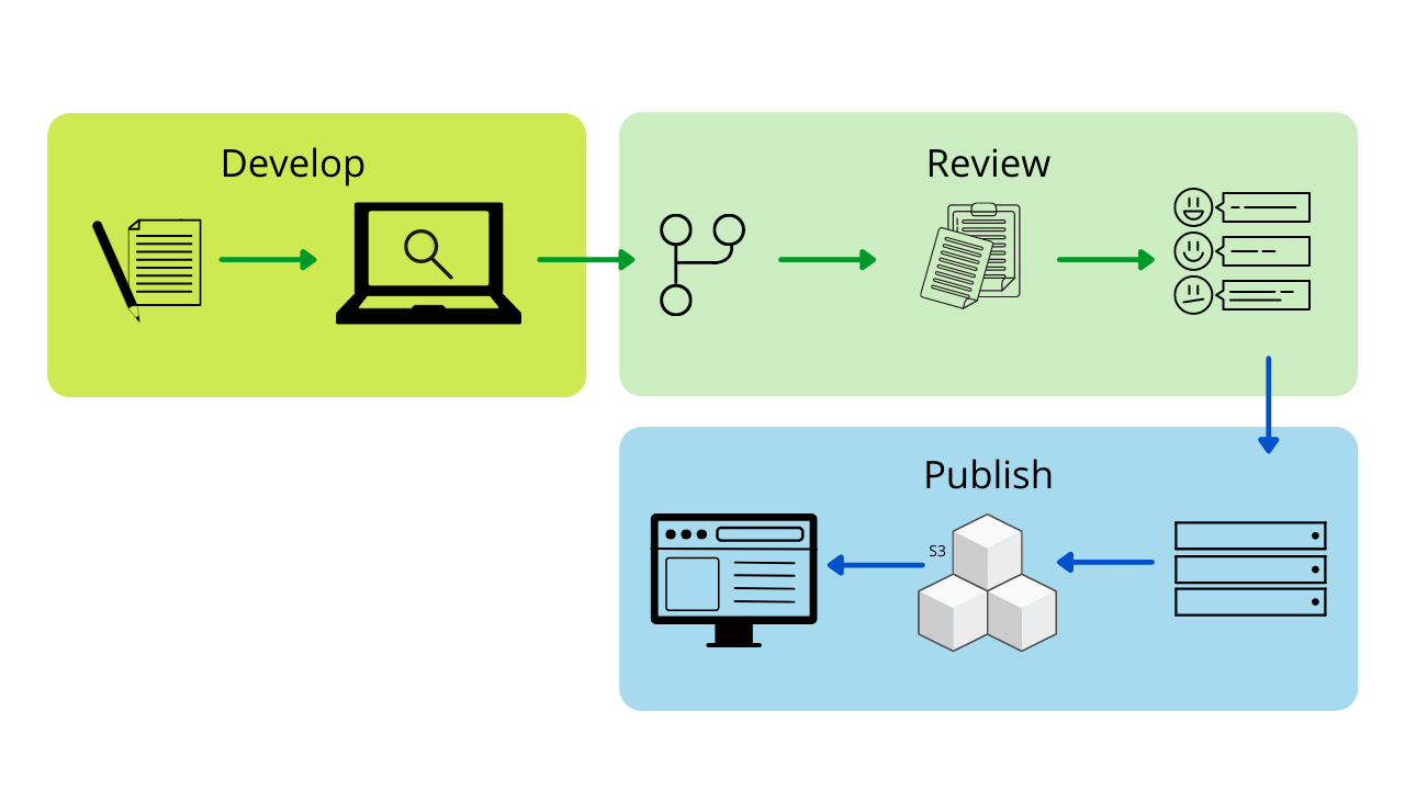
 The importance of friendly fork management
 , it takes a deeper understanding to successfully manage a fork once you have it. Management (or lack thereof) can make or break friendly forks for the following reasons:
 Our management strategies
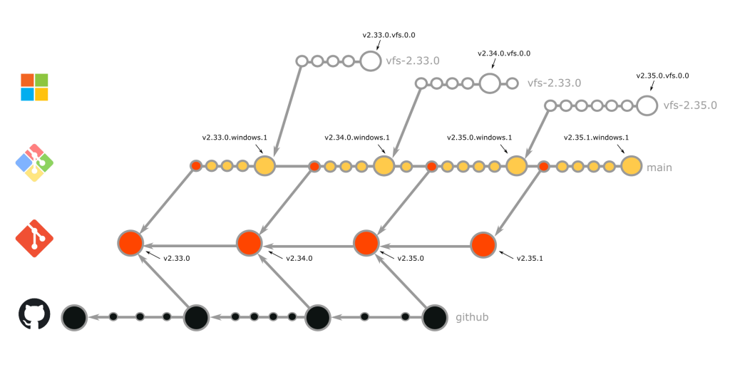
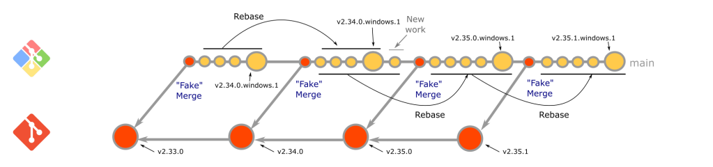
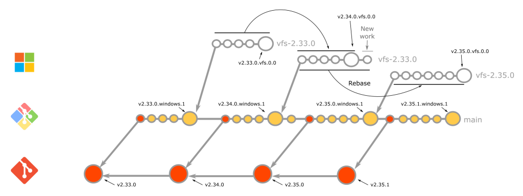
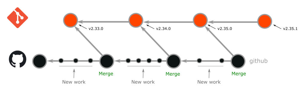
 Finding your perfect match
 Wrapping up
 To fork or not to fork
 What is a friendly fork?
 A tale of three forks
 That’s all for now!
 peeled for our second post in the “friend zone” series, in which we’ll talk about how these forks are managed and how you can adapt their strategies to your very own friendly fork!
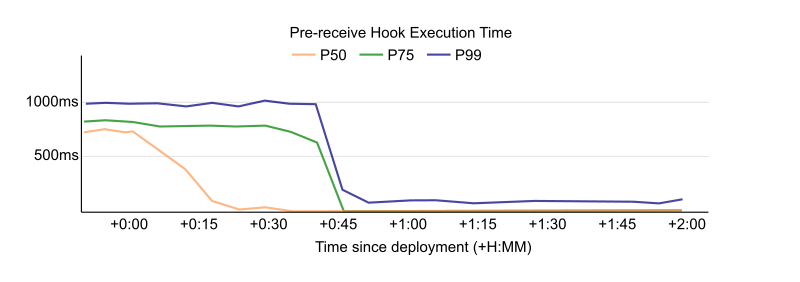
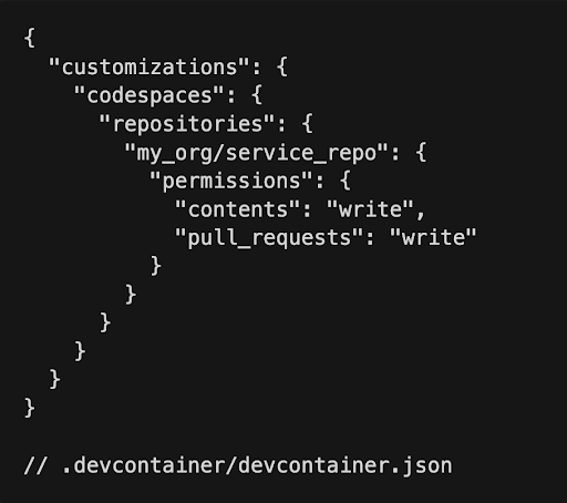
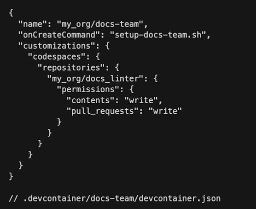

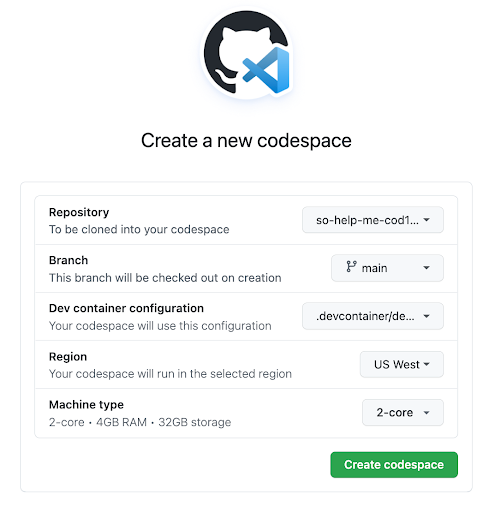


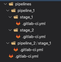
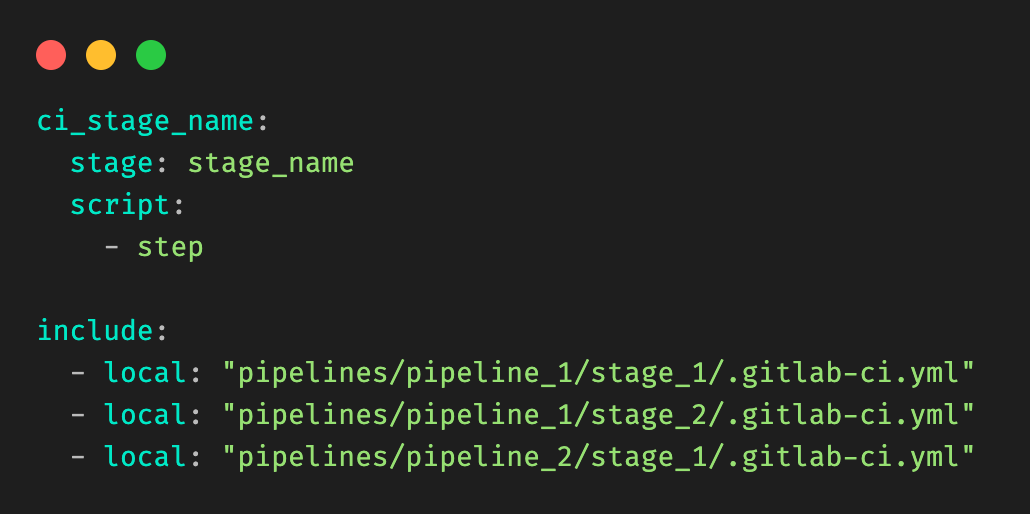
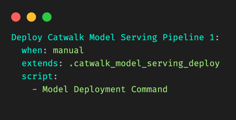
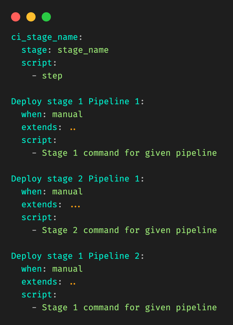
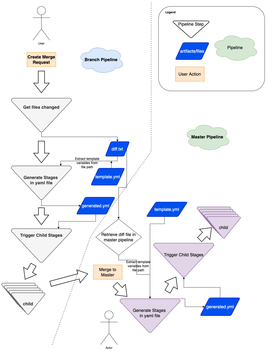
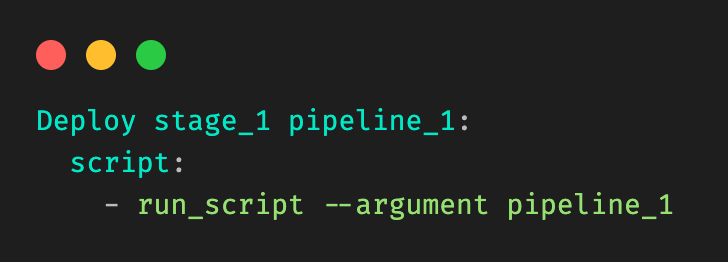
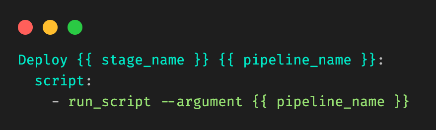

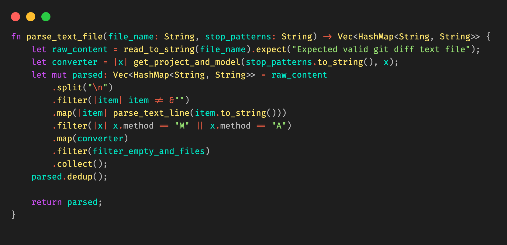
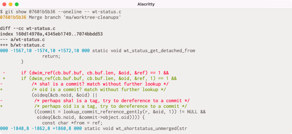
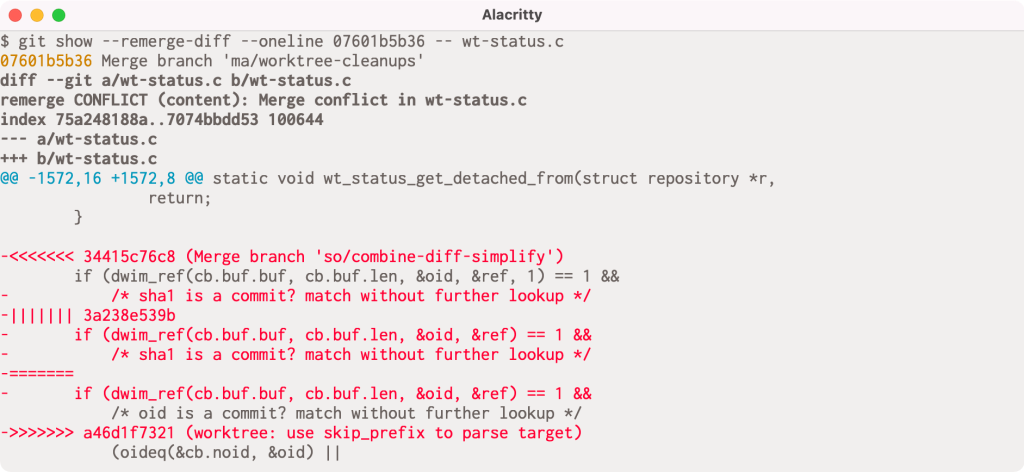

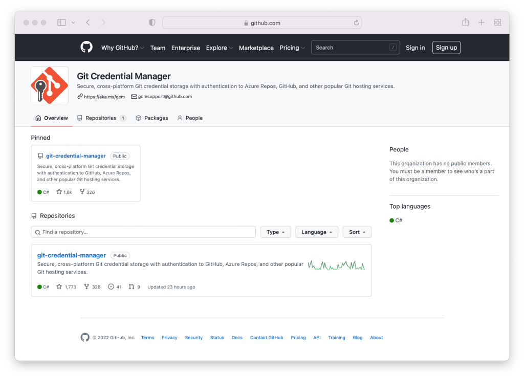

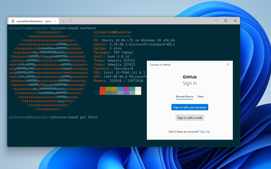
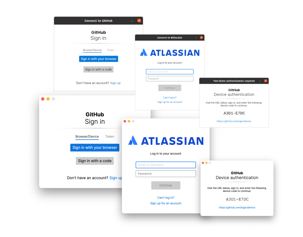

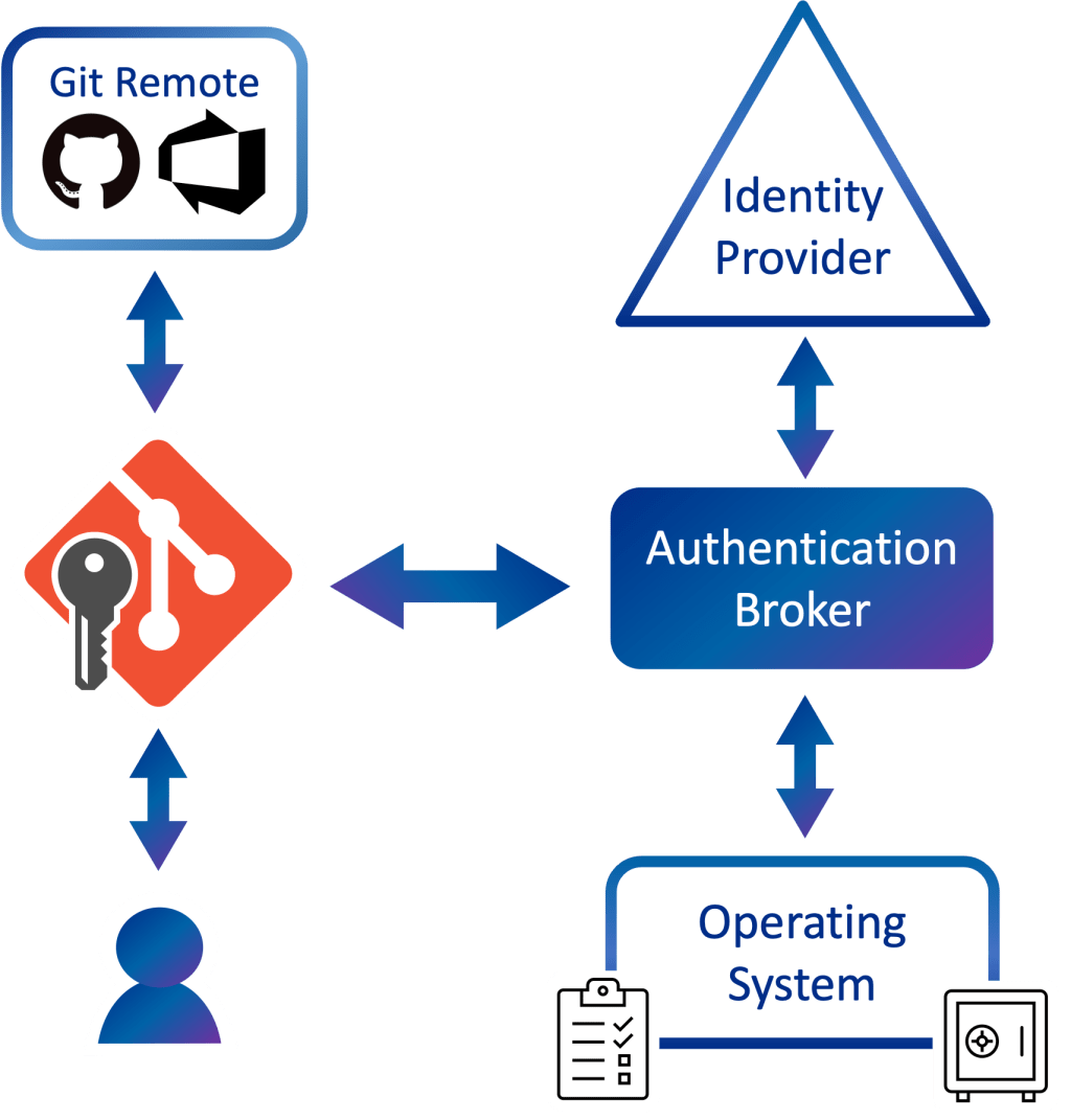

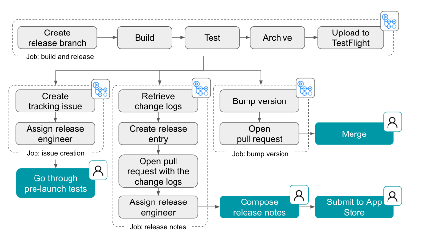
 Share company updates to GitHub’s intranet
 Create weekly reports on program status updates
 Turn weekly team photos into GIFs and upload to README