Tag Archives: news

Preview – AWS IoT RoboRunner for Building Robot Fleet Management Applications

Post Syndicated from Channy Yun original https://aws.amazon.com/blogs/aws/preview-aws-iot-roborunner-for-building-robot-fleet-management-applications/

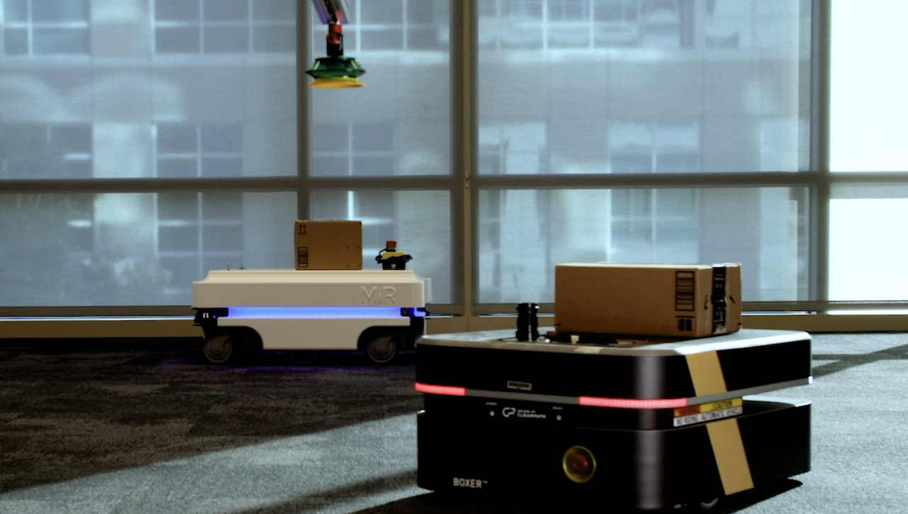
In 2018, we launched AWS RoboMaker, a cloud-based simulation service that enables robotics developers to run, scale, and automate simulation without managing any infrastructure. As we worked with robot developers and operators, we have repeatedly heard that they face challenges in operating different robot types in their automation efforts, including autonomous guided vehicles (AGV), autonomous mobile vehicles (AMR), and robotic manipulators.

Many customers choose different types of robots – often from different vendors in a single facility. Robot operator want to access the unified data required to build applications that work across a fleet of robots. However, when a new robot is added to an autonomous operation, complex and time-consuming software integration work is required to connect the robot control software to work management systems.

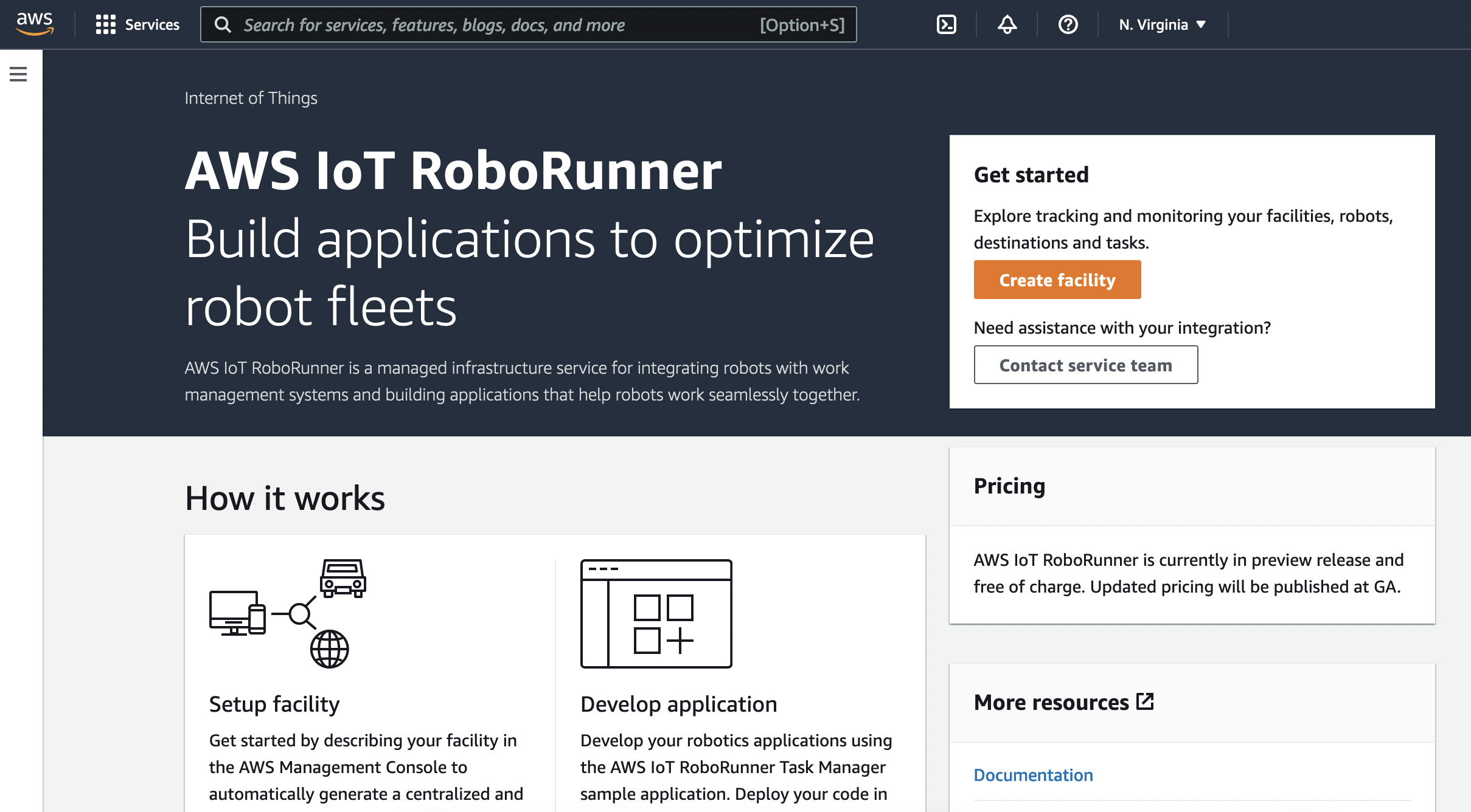
Today, we are launching a public preview of AWS IoT RoboRunner, a new robotics service that makes it easier for enterprises to build and deploy applications that help fleets of robots work seamlessly together. AWS IoT RoboRunner lets you connect your robots and work management systems, thereby enabling you to orchestrate work across your operation through a single system view.

This new service builds on the same technology used in Amazon fulfillment centers, and now we are excited to make it available to all developers to build advanced robotics applications for their businesses.

AWS IoT RoboRunner in Action
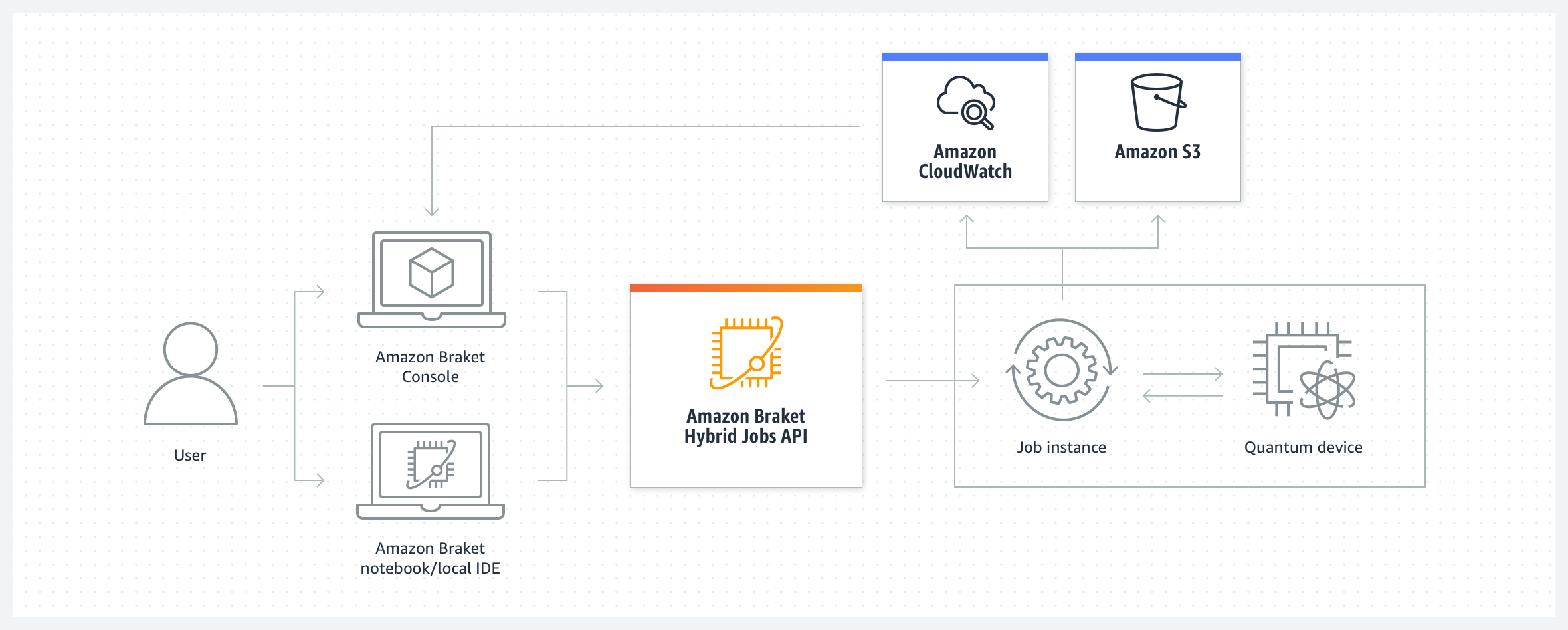
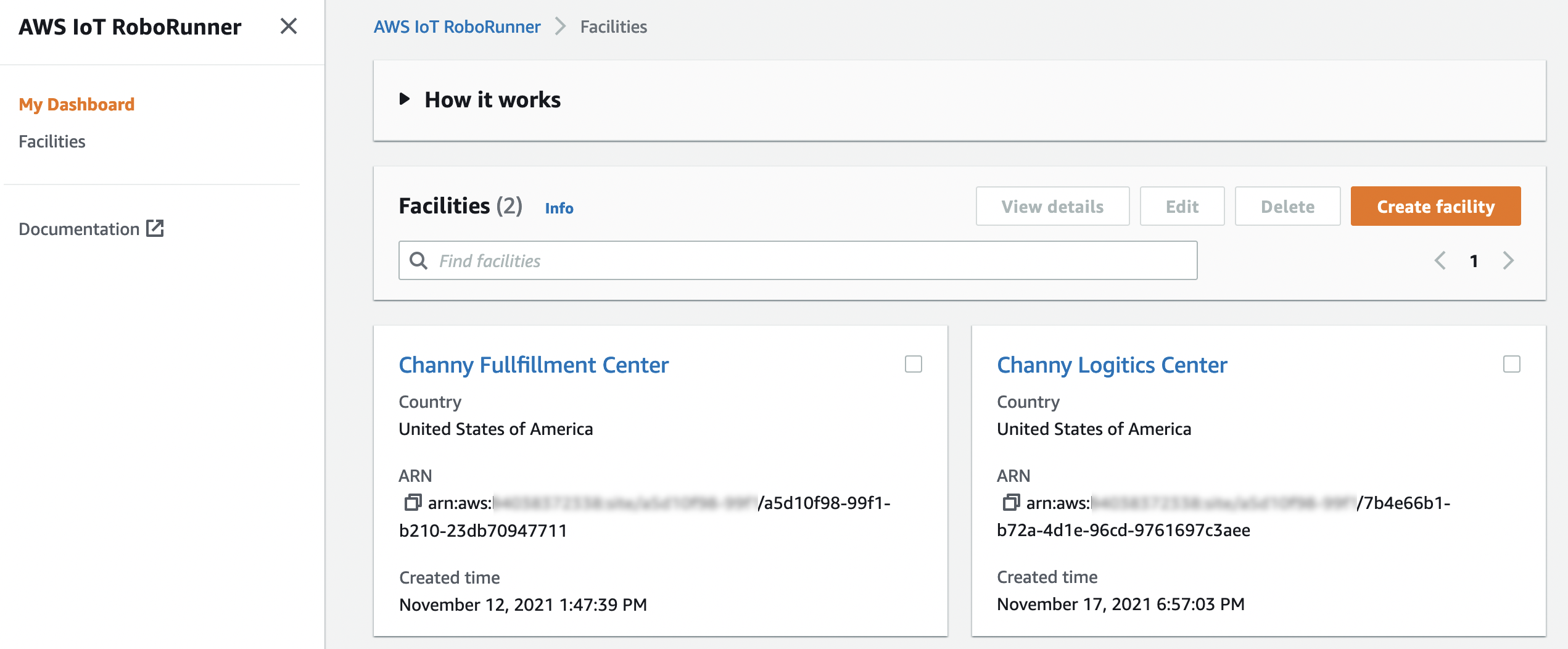
You can create a single facility (e.g., site name and location) in the AWS Management Console to get started with AWS IoT RoboRunner. Behind the scenes, AWS IoT RoboRunner automatically creates centralized repositories for storing facility, robot, destination, and task data. Then, the robots working on this site are setup as a “Fleet”, and each individual robot is setup in AWS IoT RoboRunner as a “Robot” within a fleet.

You can download the Fleet Gateway Library to develop integration codes for connecting your robots and WMS systems with AWS IoT RoboRunner to send and receive data from individual robot fleets. You can also develop the first robotics management application using the Task Manager Library and deploy Task Manager codes as an AWS Lambda function and Fleet Gateway codes on-premises as an AWS IoT Greengrass component.

To enable a single-system view of the robots, status of the systems, and progress of tasks on the same interface, AWS IoT RoboRunner provides APIs that let you build a user application. AWS IoT RoboRunner provides sample applications for allocating tasks to robot fleets so that you can get started quickly. You can customize the task allocation code with business requirements that align to your use case.

Learn more by reading Getting started with AWS IoT RoboRunner in the AWS IoT RoboRunner Developer Guide. Watch a quick introductory video about AWS IoT RoboRunner for more information.

Try Public Preview Now
AWS IoT RoboRunner is now available in public preview, and you can start using them today in the US East (N. Virginia) and Europe (Frankfrut) Regions. There will be no additional cost to use this feature during the preview period.

You can send feedback to [email protected], the AWS forum for AWS IoT, or through your usual AWS Support contacts.

— Channy

AWS Free Tier Data Transfer Expansion – 100 GB From Regions and 1 TB From Amazon CloudFront Per Month

Post Syndicated from Jeff Barr original https://aws.amazon.com/blogs/aws/aws-free-tier-data-transfer-expansion-100-gb-from-regions-and-1-tb-from-amazon-cloudfront-per-month/

The AWS Free Tier has been around since 2010 and allows you to use generous amounts of over 100 different AWS services. Some services offer free trials, others are free for the first 12 months after you sign up, and still others are always free, up to a per-service maximum. Our intent is to make it easy and cost-effective for you to gain experience with a wide variety of powerful services without having to pay any usage charges.

Free Tier Data Transfer Expansion
Today, as part of our long tradition of AWS price reductions, I am happy to share that we are expanding the Free Tier with additional data transfer out, as follows:

Data Transfer from AWS Regions to the Internet is now free for up to 100 GB of data per month (up from 1 GB per region). This includes Amazon EC2, Amazon S3, Elastic Load Balancing, and so forth. The expansion does not apply to the AWS GovCloud or AWS China Regions.

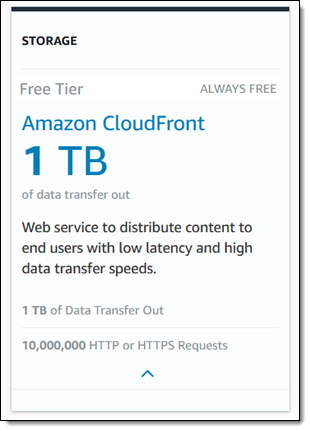
Data Transfer from Amazon CloudFront is now free for up to 1 TB of data per month (up from 50 GB), and is no longer limited to the first 12 months after signup. We are also raising the number of free HTTP and HTTPS requests from 2,000,000 to 10,000,000, and removing the 12 month limit on the 2,000,000 free CloudFront Function invocations per month. The expansion does not apply to data transfer from CloudFront PoPs in China.

This change is effective December 1, 2021 and takes effect with no effort on your part. As a result of this change, millions of AWS customers worldwide will no longer see a charge for these two categories of data transfer on their monthly AWS bill. Customers who go beyond one or both of these allocations will also see a reduction in their overall data transfer charges.

Your applications can run in any of 21 AWS Regions with a total of 69 Availability Zones (with more of both on the way), and can make use of the full range of CloudFront features (including SSL support and media streaming), and over 300 CloudFront PoPs, all connected across a dedicated network backbone. The network was designed with performance as a key driver, and is expanded continuously in order to meet the ever-growing needs of our customers. It is global, fully redundant, and built from parallel 100 GbE metro fibers linked via trans-oceanic cables across the Atlantic, Pacific, and Indian Oceans, as well as the Mediterranean, Red Sea, and South China Seas.

— Jeff;

Announcing AWS Graviton2 Support for AWS Fargate – Get up to 40% Better Price-Performance for Your Serverless Containers

Post Syndicated from Channy Yun original https://aws.amazon.com/blogs/aws/announcing-aws-graviton2-support-for-aws-fargate-get-up-to-40-better-price-performance-for-your-serverless-containers/

AWS Graviton2 processors are custom-built by AWS using 64-bit Arm Neoverse cores to deliver the best price-performance for your cloud workloads running in Amazon Elastic Compute Cloud (Amazon EC2). They provide up to 40 percent better price-performance over comparable x86-based instances for a wide variety of workloads. Many of our customers such as Intuit, SmugMug, Snap, Formula One, and Honeycomb.io use Graviton2-based instances to run their workloads for better price-performance in Amazon EC2 for their workloads and enjoy better price-performance.

Many fully-managed services including Amazon Relational Database Service (Amazon RDS), Amazon Aurora, Amazon ElastiCache, Amazon OpenSearch Service (successor of Amazon Elasticsearch Service), and Amazon EMR have extended the benefits of Graviton2 to their customers. Recently, we also extended the benefits of Graviton2 to our serverless computing customers using AWS Lambda. AWS Lambda functions powered by AWS Graviton2 offer up to 19 percent better performance at 20 percent lower cost compared to running them on x86-based instances.

Today, I am happy to announce AWS Graviton2 support for AWS Fargate with Amazon Elastic Container Service (Amazon ECS). AWS Fargate is the serverless compute engine for containers on AWS that removes the need to provision, scale, and manage servers. AWS Fargate powered by AWS Graviton2 processors delivers up to 40 percent better price-performance at 20 percent lower cost over comparable Intel x86-based Fargate for containerized applications.

With Graviton2 support for Fargate, you get the serverless benefits of Fargate, the price-performance advantages of Graviton2, and the flexibility to use a container compute processor of your choice. You can upload multi-architecture images or images that have ARM64 in your image manifest with your container registry, such as Amazon Elastic Container Registry (Amazon ECR). When orchestrated via Amazon ECS, Fargate will run these applications on Graviton2-powered compute.

Multi-architecture container images consist of two main parts: layers and a manifest. Each container image has one or more layers of file system content. The manifest specifies the groups of layers that make up the image as well as its runtime characteristics, either ARM64 and X86_64.

This allows you to have the same repository that supports multiple architectures, and the container runtime does the work of selecting which image layers to pull based on the system architecture, including ARM64. To learn more, visit Introducing multi-architecture container images for Amazon ECR.

Getting Started With Fargate powered by Graviton2 processors
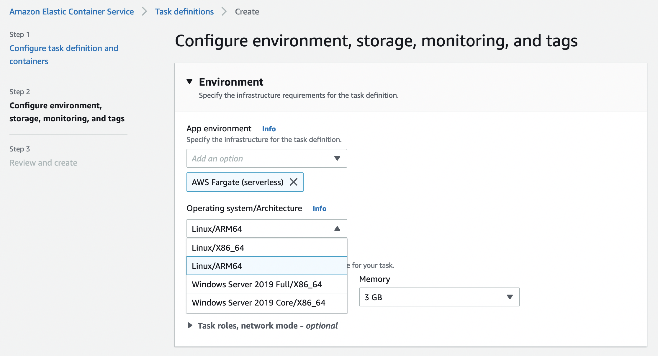
To enable Graviton2 support for Fargate, you opt in to Arm compatibility in your ECS cluster. In the ECS console, when creating a new task definition, you can simply select Linux/ARM64 in the Operating system/Architecture dropdown list.

The following is an example of a task definition containing a simple container using the Fargate launch type with an optional parameter cpuArchitecture to ARM64. (The default value is X86_64).

{
 "family": "bb-arm64",
 "networkMode": "awsvpc",
 "containerDefinitions": [
    {
        "name": "sleep",
        "image": "arm64v8/busybox",
        "cpu": 100,
        "memory": 100,
        "essential": true,
        "command": [ "echo hello" ],
        "entryPoint": [ "sh", "-c" ]
    }
 ],
 "requiresCompatibilities": [ "FARGATE" ],
 "cpu": "1 vCpu",
 "memory": "3 GB",
 "runtimePlatform": { "cpuArchitecture": "ARM64" },
 "executionRoleArn": "arn:aws:iam::1234567890:role/ecsTaskExecutionRole"
}

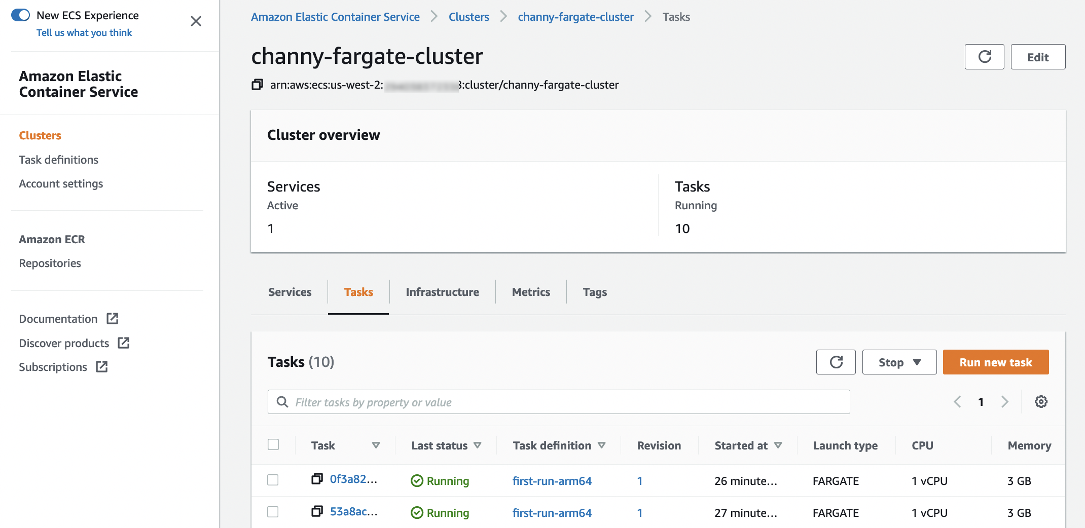
When you run your tasks with the Graviton-based compute, you can see the value of Linux/ARM64 for Operating system/Architecture in each task detail page of the ECS console.

With AWS Command-line Interface (AWS CLI), you simply find which architecture is used in your ECS cluster.

$ aws ecs describe-tasks \
    --cluster MyCluster \
    --tasks arn:aws:ecs:us-west-2:123456789012:task/MyCluster/1234567890123456789

Here is an output of CPU architecture in the response of DescribeTasks or will have it as a filter to ListTasks.

{ 
    "tasks": [
    {
        "family": "...",
        "attributes": [
            {
                "name": "ecs.cpu-architecture",
                "value": "arm64"
            }
        ]
    }]
}

Migration to Gaviton2-based Fargate Containers
You get all the same Fargate features you’re used to for your containerized applications with Intel x86-based offering. With logging, monitoring, tracing, extensible ephemeral storage by Amazon Elastic File System (Amazon EFS) file systems, and more, you can easily migrate your applications to Graviton2-based Fargate containers. You get out-of-the-box logging via Amazon CloudWatch logs and metrics via Container Insights and AWS Distro for Open Telemetry agent as a sidecar to enable traces via ServiceLens.

With Amazon ECS, you can use Amazon ECS Exec for break-glass or developer debugging scenarios. With ECS Exec, you can directly interact with containers without needing to first interact with the host container operating system, open inbound ports, or manage SSH keys. You can use ECS Exec to run commands in or get a shell to a container running on an Amazon EC2 instance or on AWS Fargate.  To learn more, see Using Amazon ECS Exec for debugging in the AWS documentation.

Once your development teams test and validate that applications are ARM64 compatible, in addition to using AWS CodeBuild that has supported Graviton for a long time, you can now run Jenkins or Gitlab runners. This will give you an end-to-end serverless experience, right from testing to building containers to running them on Fargate.

To get more support with the monitoring and logging, security, and continuous delivery on AWS Fargate, see the list of AWS Fargate Partners such as Aqua Security, Datadog, New Relic, Splunk, and Sumo Logic that have extended Fargate’s capabilities.

Available Now
AWS Graviton2 support on AWS Fargate is available in all AWS Regions where Fargate is available except Bahrain, Cape Town, China, and GovCloud regions. This feature is supported on Fargate Platform Version (PV) 1.4.0 or later. If you are not already using PV 1.4.0, see the AWS Fargate platform versions section in the AWS documentation to learn how to migrate.

You can get up to 40 percent better price-performance for Arm-compatible container-based applications. You can further reduce your costs by getting up to a 52 percent discount off on-demand pricing in exchange for a commitment of a one- or three-year term with Compute Savings Plans. For more information, see the AWS Fargate pricing page.

Give it a try, and please send us feedback either on the public AWS containers roadmap in the AWS forum for Amazon ECS, or through your usual AWS support contacts.

– Channy

AWS Cloud Adoption Framework (CAF) 3.0 is Now Available

Post Syndicated from Jeff Barr original https://aws.amazon.com/blogs/aws/aws-cloud-adoption-framework-caf-3-0-is-now-available/

The AWS Cloud Adoption Framework (AWS CAF) is designed to help you to build and then execute a comprehensive plan for your digital transformation. Taking advantage of AWS best practices and lessons learned from thousands of customer engagements, the AWS CAF will help you to identify and prioritize transformation opportunities, evaluate and improve your cloud readiness, and iteratively evolve the roadmaps that you follow to guide your transformation.

Version 3.0 Now Available
I am happy to announce the version 3.0 of the AWS CAF is now available. This version represents what we have learned since we released version 2.0, with a focus on digital transformation and an emphasis on the use of data & analytics.

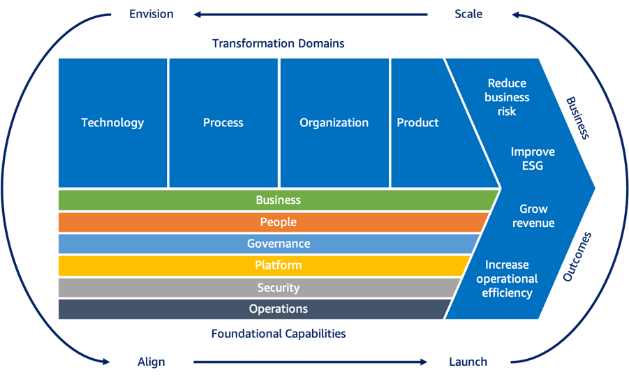
The framework starts by identifying six groups of foundational perspectives (Business, People, Governance, Platform, Security, and Operations), totaling 47 discrete capabilities, up from 31 in the previous version.

From there it identifiers four transformation domains (Technology, Process, Organization, and Product) that must participate in a successful digital transformation.

With the capabilities and the transformation domains as a base, the AWS Cloud Adoption Framework then recommends a set of four iterative and incremental cloud transformation phases:

Envision – Demonstrate how the cloud will accelerate business outcomes. This phase is delivered as a facilitator-led interactive workshop that will help you to identify transformation opportunities and create a foundation for your digital transformation.

Align – Identify capability gaps across the foundational capabilities. This phase also takes the form of a facilitator-led workshop and results in an action plan.

Launch – Build and deliver pilot initiatives in production, while demonstrating incremental business value.

Scale – Expand pilot initiatives to the desired scale while realizing the anticipated & desired business benefits.

All in all, the AWS Cloud Adoption Framework is underpinned by hundreds of AWS offerings and programs that help you achieve specific business and technical outcomes.

Getting Started with the AWS Cloud Adoption Framework
You can use the following resources to learn more and to get started:

Web Page – Visit the AWS Cloud Adoption Framework web page.

White Paper – Download and read the AWS CAF Overview.

AWS Account Team – Your AWS account team stands ready to assist you with any and all of the phases of the AWS Cloud Adoption Framework.

— Jeff;

New – Amazon EC2 R6i Memory-Optimized Instances Powered by the Latest Generation Intel Xeon Scalable Processors

Post Syndicated from Danilo Poccia original https://aws.amazon.com/blogs/aws/new-amazon-ec2-r6i-memory-optimized-instances-powered-by-the-latest-generation-intel-xeon-scalable-processors/

In August, we introduced the general-purpose Amazon EC2 M6i instances powered by the latest generation Intel Xeon Scalable processors (code-named Ice Lake) with an all-core turbo frequency of 3.5 GHz. Compute-optimized EC2 C6i instances were also made available last month.

Today, I am happy to share that we are expanding our sixth-generation x86-based offerings to include memory-optimized Amazon EC2 R6i instances.

Here’s a quick recap of the advantages of the new R6i instances compared to R5 instances:

  • A larger instance size (r6i.32xlarge) with 128 vCPUs and 1,024 GiB of memory that makes it easier and more cost-efficient to consolidate workloads and scale up applications
  • Up to 15 percent improvement in compute price/performance
  • Up to 20 percent higher memory bandwidth
  • Up to 40 Gbps for Amazon Elastic Block Store (EBS) and 50 Gbps for networking which is 2x more than R5 instances
  • Always-on memory encryption.

R6i instances are SAP Certified and are an ideal fit for memory-intensive workloads such as SQL and NoSQL databases, distributed web scale in-memory caches like Memcached and Redis, in-memory databases, and real-time big data analytics like Apache Hadoop and Apache Spark clusters.

Compared to M6i and C6i instances, the only difference is in the amount of memory that is included per vCPU. R6i instances are available in ten sizes:

Name vCPUs Memory
(GiB)
Network Bandwidth
(Gbps)
EBS Throughput
(Gbps)
r6i.large 2 16 Up to 12.5 Up to 10
r6i.xlarge 4 32 Up to 12.5 Up to 10
r6i.2xlarge 8 64 Up to 12.5 Up to 10
r6i.4xlarge 16 128 Up to 12.5 Up to 10
r6i.8xlarge 32 256 12.5 10
r6i.12xlarge 48 384 18.75 15
r6i.16xlarge 64 512 25 20
r6i.24xlarge 96 768 37.5 30
r6i.32xlarge 128 1024 50 40
r6i.metal 128 1024 50 40

Like M6i and C6i instances, these new R6i instances are built on the AWS Nitro System, which is a collection of building blocks that offloads many of the traditional virtualization functions to dedicated hardware, delivering high performance, high availability, and highly secure cloud instances.

As with all sixth generation EC2 instances, you may need to upgrade your Elastic Network Adapter (ENA) for optimal networking performance. For more information, see this article about migrating an EC2 instance to a sixth-generation instance in the AWS Knowledge Center.

R6i instances support Elastic Fabric Adapter (EFA) on r6i.32xlarge and r6i.metal instances for workloads that benefit from lower network latency, such as HPC and video processing.

Availability and Pricing
EC2 R6i instances are available today in four AWS Regions: US East (N. Virginia), US West (Oregon), US East (Ohio), Europe (Ireland). As usual with EC2, you pay for what you use. For more information, see the EC2 pricing page.

— Danilo

Scalable, Cost-Effective Disaster Recovery in the Cloud

Post Syndicated from Steve Roberts original https://aws.amazon.com/blogs/aws/scalable-cost-effective-disaster-recovery-in-the-cloud/

Should disaster strike, business continuity can require more than just periodic data backups. A full recovery that meets the business’s recovery time objectives (RTOs) must also include the infrastructure, operating systems, applications, and configurations used to process their data. The growing threats of ransomware highlight the need to be able to perform a full point-in-time recovery. For businesses affected by a ransomware attack, restoration of data from an old, possibly manual, backup will not be sufficient.

Previously, businesses have elected to provision separate, physical disaster recovery (DR) infrastructure. However, customers tell us this can be both space- and cost-prohibitive, involving capital expenditure on hardware and facilities that remain idle until called upon. The infrastructure also incurs overhead in terms of regular inspection and maintenance, typically manual, to ensure that should it ever be called upon, it’s ready and able to handle the current business load, which may have grown considerably since initial provisioning. This also makes testing difficult and expensive.

Today, I am happy to announce AWS Elastic Disaster Recovery (DRS) a fully scalable, cost-effective disaster recovery service for physical, virtual, and cloud servers, based on CloudEndure Disaster Recovery. DRS enables customers to use AWS as an elastic recovery site without needing to invest in on-premises DR infrastructure that lies idle until needed. Once enabled, DRS maintains a constant replication posture for your operating systems, applications, and databases. This helps businesses meet recovery point objectives (RPOs) of seconds, and RTOs of minutes, after disaster strikes. In cases of ransomware attacks, for example, DRS also allows recovery to a previous point in time.

DRS provides for recovery that scales as needed to match your current setup and does not need any time-consuming manual processes to maintain that readiness. It also offers the ability to perform disaster recovery readiness drills. Just as it’s important to test restoration of data from backups, being able to conduct recovery drills in a cost-effective manner without impacting ongoing replication or user activities can help give confidence that you can meet your objectives and customer expectations should you need to call on a recovery.

AWS Elastic Disaster Recovery console home

Elastic Disaster Recovery in Action
Once enabled, DRS continuously replicates block storage volumes from physical, virtual, or cloud-based servers, allowing it to support business RPOs measured in seconds. Recovery includes applications running on physical infrastructure, VMware vSphere, Microsoft Hyper-V, and cloud infrastructure to AWS. You’re able to recover all your applications and databases that run on supported Windows and Linux operating systems, with DRS orchestrating the recovery process for your servers on AWS to support an RTO measured in minutes.

Using an agent that you install on your servers, DRS securely replicates the data to a staging area subnet in a selected Region in your AWS account. The staging area subnet reduces costs to you, using affordable storage and minimal compute resources. Within the DRS console, you can recover Amazon Elastic Compute Cloud (Amazon EC2) instances in a different AWS Region if required. With DRS automating replication and recovery procedures, you can set up, test, and operate your disaster recovery capability using a single process without the need for specialized skill sets.

DRS gives you the flexibility to pay on an hourly basis, instead of needing to commit to a long-term contract or a set number of servers, a benefit over on-premises or data center recovery solutions. DRS charges hourly, on a pay-as-you-go basis. You can find specific details on pricing at the product page.

Exploring Elastic Disaster Recovery
To set up disaster recovery for my resources I first need to configure my default replication settings. As I mentioned earlier, DRS can be used with physical, virtual, and cloud servers. For this post, I’m going to use a collection of EC2 instances as my source servers for disaster recovery.

From the DRS console home, shown earlier, choosing Set default replication settings takes me to a short initialization wizard. In the wizard, I first need to select an Amazon Virtual Private Cloud (VPC) subnet that will be used for staging. This subnet does not need to be in the same VPC as my resources, but I need to select one that is not private or blocked to the world. Below, I’ve chosen a subnet from my default VPC in my Region. I can also change the instance type used for the replication instance. I chose to keep the suggested default and clicked Next to proceed.

Choosing the staging area subnet and replication instance type for DRS

I also left the default settings unchanged for the next two pages. In Volumes and security groups, the wizard suggests I use the general-purpose SSD (gp3) Amazon Elastic Block Store (EBS) storage type and to use a security group provided by DRS. On the Additional settings page I can elect to use a private IP for data replication instead of routing over the public internet, and set the snapshot retention period, which defaults to seven days. Clicking Next one final time, I arrive at the Review and create page of the wizard. Choosing Create default completes the process of configuring my default replication settings.

Finalizing default replication settings for DRS

With my replication settings finalized (I can edit them later if I wish, from the Actions menu on the Source servers console page) it’s time to set up my servers. I’m running a test fleet in EC2 that includes two Windows Server 2019 instances, and three Amazon Linux 2 instances. The DRS User Guide contains full instructions on how to obtain and set up the agent on each server type, so I won’t repeat them here. As I run and configure the agent on each of my server instances, the Source servers list automatically updates to include the new source server. The status of the initial sync, and future replication and recovery status of each source server, are summarized in this view.

Replication sync activity on servers

Selecting a hostname entry in the list takes me to a detail page. Here I can view a recovery dashboard, information on the underlying server, disk settings (including the ability to change the staging disk type from the default gp3 type selected by the initialization wizard, or whatever you choose during setup), and launch settings, shown below, that govern the recovery instance that will be created if I choose to initiate a drill or an actual recovery job.

DRS launch settings for a recovery server

Just like data backups, where established best practice is to periodically verify that the backups can actually be used to restore data, we recommend a similar best practice for disaster recovery. So, with my servers all configured and fully replicated, I decided to start a drill for a point-in-time (PIT) recovery for two of my servers. On these instances, following initial replication, I’d installed some additional software. In my scenario, perhaps this installation had gone badly wrong, or I’d fallen victim to a ransomware attack. Either way, I wanted to know and be confident that I could recover my servers if and when needed.

In the Source servers list I selected the two servers that I’d modified and from the Initiate recovery job drop-down menu, chose Initiate drill. Next, I can choose the recovery PIT I’m interested in. This view defaults to Any, meaning it lists all recovery PIT snapshots for the servers I selected. Or, I can choose to filter to All, meaning only PIT snapshots that apply to all the selected servers will be listed. Selecting All, I chose a time just after I’d completed installing additional software on the instances, and clicked Initiate drill.

Selecting a recovery point-in-time for multiple servers

I’m returned to the Source servers list, which shows status as the recovery proceeds. However, I switched to the Recovery job history view for more detail.

In-progress recovery drill

Clicking the job ID, I can drill down further to view a detail page of the source servers involved in the recovery (and can drill down further for each), as well as an overall recovery job log.

Viewing the recovery job log

Note – during a drill, or an actual recovery, if you go to the EC2 console you’ll notice one or more additional instances, started by DRS, running in your account (in addition to the replication server). These temporary instances, named AWS Elastic Disaster Recovery Conversion Server, are used to process the PIT snapshots onto the actual recovery instance(s) and will be terminated when the job is complete.

Once the recovery is complete, I can see two new instances in my EC2 environment. These are in the state matching the point-in-time recovery I selected, and are using the instance types I selected earlier in the DRS initialization wizard. I can now connect to them to verify that the recovery drill performed as expected before terminating them. Had this been a real recovery, I would have the option of terminating the original instances to replace them with the recovery versions, or handle whatever other tasks are needed to complete the disaster recovery for my business.

New instances matching my point-in-time recovery selection

Set Up Your Disaster Recovery Environment Today
AWS Elastic Disaster Recovery is generally available now in the US East (N. Virginia), US East (Ohio), US West (Oregon), Asia Pacific (Singapore), Asia Pacific (Sydney), Asia Pacific (Tokyo), Europe (Frankfurt), Europe (Ireland), and Europe (London) Regions. Review the AWS Elastic Disaster Recovery User Guide for more details on setup and operation, and get started today with DRS to eliminate idle recovery site resources, enjoy pay-as-you-go billing, and simplify your deployments to improve your disaster recovery objectives.

— Steve

Meet the latest AWS Heroes – November 2021

Post Syndicated from Ross Barich original https://aws.amazon.com/blogs/aws/meet-the-latest-aws-heroes-november-2021/

It is an exciting time of year, with AWS re:Invent right around the corner. As we reflect back on 2021, we continue to be impressed by the way AWS communities support one-another across intersecting journeys to expand technical skills. At the center of these communities are impactful leaders who go above and beyond to create educational content and facilitate peer-to-peer knowledge sharing across multiple channels. These passionate builders are called AWS Heroes, and we are humbled by the amazing activities they support on behalf of their communities. Today we are excited to introduce the latest cohort of AWS Heroes:

Juan Pan – Beijing, China

Data Hero Juan Pan (Trista) is the CTO and Co-Founder of SphereEx. She serves as an Apache ShardingSphere Project Management Committee member, as well as a mentor on various other Apache incubation projects. She was a recipient of the 2020 and 2021 “China OSCAR Open Source Pioneer” award, and frequently speaks at relevant conferences in the fields of databases & database architecture, including at AWS Summit Shanghai and AWS Dev Days. Juan loves to encourage more women to pursue careers in technology, and she regularly shares her empowering journey from open source contributor to CTO at events such as the AWS She Builds Summit.

Masanori Yamaguchi – Chiba, Japan

Community Hero Masanori Yamaguchi is a Solution Architect at KDDI Corporation. Yamaguchi joined the Japanese AWS User Group (JAWS-UG) in 2014 and has since managed 35 events including the reboot of Fin-JAWS (Financial-JAWS), and the JAWS-UG Chiba Chapter in 2019. Yamaguchi organized the 2021 JAWS-UG online event (JAWS DAYS 2021). This event was a new challenge in online events: not only delivering sessions, but also providing a place for attendees to communicate with each other and participate in AWS quizzes, games, and more. 4,000 participants from all over Japan attended the event. In recognition of these activities, he received the AWS Samurai 2020 Award.

Pamela Gotti – Milan, Italy

Community Hero Pamela Gotti is Chief Technology Officer at Credimi. She loves to design systems with clear boundaries through domain-driven design and event storming, and to bring them to life on Amazon EKS, with a mix of AWS Lambda, Amazon RDS, and Amazon S3. She has given talks about how Credimi uses AWS to implement new features, microservices communication approaches (from event-driven architecture to GraphQL), and about team organization. Since 2018 Pamela has led the tech team of SheTech, organizing events that help women build coding skills. The coding bootcamps focus on machine learning with Python, web development with JavaScript, and serverless.

Salah Elhossiny – Cairo, Egypt

Machine Learning Hero Salah Elhossiny works as an ML full stack developer, building backend and frontend solutions integrated with ML pipelines to provide intelligence for data labeling and analysis processes. Salah also builds serverless solutions on AWS integrated with ML models on Amazon SageMaker. A certified AWS ML specialist, Salah is an involved member of the AWS MENA Community, where he frequently writes summaries of AWS whitepapers to facilitate AWS certification exam preparation for fellow community members. He also enjoys writing about machine learning on Amazon SageMaker and serverless solutions.

Sheng Wu – Beijing, China

Container Hero Sheng Wu is a founding engineer at Tetrate. He serves on the world’s biggest open source foundation, The Apache Software Foundation, as a board director and mentor of the incubator. He is a regular speaker at conferences such as the AWS Summit, AWS Dev Day, QCon, KubeCon, and ApacheCon, typically sharing his expertise in observability for container-based and cloud-native environments. His articles and blogs on containers, cloud-native, and observability appear in media including The New Stack and the Apache SkyWalking Official Blog.

Takahiro Horike – Tokyo, Japan

Serverless Hero Takahiro Horike is CEO of Serverless Operations, Inc. While working in cloud computing, he participates in and contributes to the open source community, letting people know how fun and meaningful it is by speaking at AWS official events like AWS Dev Day. He also speaks at Japan AWS User Group (JAWS-UG) events. Horike has contributed to several open source projects on GitHub, including Serverless Step Functions. His nearly 40 presentations can be found on SlideShare and Speaker Deck.

Vanessa Santos – São Paulo, Brazil

Community Hero Vanessa Santos joined the AWS User Group São Paulo in 2017. Starting from a non-traditional technical background, she became recognized as an AWS Community Leader in 2019, achieving new learnings and practices through the AWS re:Invent We Power Tech Grant. Passionate about technology, Vanessa believes people can continuously learn and still be curious for more. She works with local and international AWS User Groups as an AWS UG São Paulo co-organizer, with female and black tech communities, as an MBA Lecturer, and as council volunteer for Brazilian health tech.

Vivek Raja P S – Madurai, India

Machine Learning Hero Vivek Raja works as Data Scientist at NexStem | CortexBCI Inc. He is an active speaker where he shares his learnings with AWS User Group India, at events such as AWS Community Day ANZ, and at various developer communities including the TensorFlow User Group, and Women in Data Science. He also supports AWS re:Skill with technical talks, podcasts, and open-source projects. Vivek regularly writes blogs where he shares about AWS Machine Learning and AWS DeepRacer. He is a DeepRacer enthusiast and uses it to help students learn Machine Learning by organizing regional AWS DeepRacer contests.

If you’d like to learn more about the new Heroes, or connect with a Hero near you, please visit the AWS Heroes website or browse the AWS Heroes Content Library.

— Ross;

New – EC2 Instances (G5) with NVIDIA A10G Tensor Core GPUs

Post Syndicated from Jeff Barr original https://aws.amazon.com/blogs/aws/new-ec2-instances-g5-with-nvidia-a10g-tensor-core-gpus/

Two years ago I told you about the then-new G4 instances, which featured up to eight NVIDIA T4 Tensor Core GPUs. These instances were designed to give you cost-effective GPU power for machine learning inference and graphics-intensive applications.

Today I am happy to tell you about the new G5 instances, which feature up to eight NVIDIA A10G Tensor Core GPUs. Powered by second generation AMD EPYC processors, these instances deliver up to 40% better price-performance for inferencing and graphics-intensive operations in comparison to their predecessors.

On the GPU side, the A10G GPUs deliver to to 3.3x better ML training performance, up to 3x better ML inferencing performance, and up to 3x better graphics performance, in comparison to the T4 GPUs in the G4dn instances. Each A10G GPU has 24 GB of memory, 80 RT (ray tracing) cores, 320 third-generation NVIDIA Tensor Cores, and can deliver up to 250 TOPS (Tera Operations Per Second) of compute power for your AI workloads.

Here are the specs:

Instance Name
NVIDIA A10G
Tensor Core GPUs
vCPUs Memory Local Storage EBS Bandwidth Network Bandwidth
g5.xlarge 1 4 16 GiB 250 GB Up to 3.5 Gbps Up to 10 Gbps
g5.2xlarge 1 8 32 GiB 450 GB Up to 3.5 Gbps Up to 10 Gbps
g5.4xlarge 1 16 64 GiB 600 GB 8 Gbps Up to 25 Gbps
g5.8xlarge 1 32 128 GiB 1900 GB 16 Gbps 25 Gbps
g5.12xlarge 4 48 192 GiB 3800 GB 16 Gbps 40 Gbps
g5.16xlarge 1 64 256 GiB 1900 GB 16 Gbps 25 Gbps
g5.24xlarge 4 96 384 GiB 3800 GB 19 Gbps 50 Gbps
g5.48xlarge 8 192 768 GiB 7600 GB 19 Gbps 100 Gbps

Like their predecessors, these instances are a great fit for many interesting types of workloads. Here are a few examples:

Media and Entertainment – Customers can use G5 instances to support finishing and color grading tasks, generally with the aid of high-end pro-grade tools. These tasks can also support real-time playback, aided by the plentiful amount of EBS bandwidth allocated to each instance. Customers can also use the increased ray-tracing power of G5 instances to support game development tools.

Remote Workstations – Customers in many different industries including Media and Entertainment, Gaming, Education, Architecture, Engineering and Construction want to run high-end graphical workstations in the cloud, and are looking for instances that come in a broad array of sizes.

Machine & Deep Learning – G5 instances deliver high performance and significant value for training and inferencing workloads. They also offer access to NVIDIA CuDNN, NVIDIA TensorRT, NVIDIA Triton Inference Server, and other ML/DL software from the NVIDIA NGC catalog, which have all been optimized for use with NVIDIA GPUs.

Autonomous Vehicles – Several of our customers are designing and simulating autonomous vehicles that include multiple real-time sensors. The customers make use of ray tracing to simulate sensor input in real time, and also gather data from real-world tests using tools that benefit from powerful networking and large amounts of memory.

The instances support Linux and Windows, and are compatible with a very long list of graphical and machine learning libraries including CUDA, CuDNN, CuBLAS, NVENC, TensorRT, OpenCL, DirectX, Vulkan, and OpenGL.

Available Now
The new G5 instances are available now and you can start using them today in the US East (N. Virginia), US West (Oregon), and Europe (Ireland) Regions in On-Demand, Spot, Savings Plan, and Reserved Instance form. You can also launch them in Amazon Elastic Container Service (Amazon ECS) and Amazon Elastic Kubernetes Service (EKS) clusters,

To learn more, check out the G5 Instances page.

— Jeff;

Measure and Improve Your Application Resilience with AWS Resilience Hub

Post Syndicated from Sébastien Stormacq original https://aws.amazon.com/blogs/aws/monitor-and-improve-your-application-resiliency-with-resilience-hub/

I am excited to announce the immediate availability of AWS Resilience Hub, a new AWS service designed to help you define, track, and manage the resilience of your applications.

You are building and managing resilient applications to serve your customers. Building distributed systems is hard; maintaining them in an operational state is even harder. The question is not if a system will fail, but when it will, and you want to be prepared for that.

Resilience targets are typically measured by two metrics: Recovery Time Objective (RTO), the time it takes to recover from a failure, and Recovery Point Objective (RPO), the maximum window of time in which data might be lost after an incident. Depending on your business and application, these can be measured in seconds, minutes, hours, or days.

AWS Resilience Hub lets you define your RTO and RPO objectives for each of your applications. Then it assesses your application’s configuration to ensure it meets your requirements. It provides actionable recommendations and a resilience score to help you track your application’s resiliency progress over time. Resilience Hub gives a customizable single dashboard experience, accessible through the AWS Management Console, to run assessments, execute prebuilt tests, and configure alarms to identify issues and alert the operators.

AWS Resilience Hub discovers applications deployed by AWS CloudFormation (this includes SAM and CDK applications), including cross Regions and cross account stacks. Resilience Hub also discovers applications from Resource Groups and tags or chooses from applications already defined in AWS Service Catalog AppRegistry.

The term “application” here refers not just to your application software or code; it refers to the entire infrastructure stack to host the application: networking, virtual machines, databases, and so on.

Resilience assessment and recommendations
AWS Resilience Hub’s resilience assessment utilizes best practices from the AWS Well-Architected Framework to analyze the components of your application and uncover potential resilience weaknesses caused by incomplete infrastructure setup, misconfigurations, or opportunities for additional configuration improvements. Resilience Hub provides actionable recommendations to improve the application’s resilience.

For example, Resilience Hub validates that the application’s Amazon Relational Database Service (RDS), Amazon Elastic Block Store (EBS), and Amazon Elastic File System (Amazon EFS) backup schedule is sufficient to meet the application’s RPO and RTO you defined in your resilience policy. When insufficient, it recommends improvements to meet your RPO and RTO objectives.

The resilience assessment generates code snippets that help you create recovery procedures as AWS Systems Manager documents for your applications, referred to as standard operating procedures (SOPs). In addition, Resilience Hub generates a list of recommended Amazon CloudWatch monitors and alarms to help you quickly identify any change to the application’s resilience posture once deployed.

Continuous resilience validation
After the application and SOPs have been updated to incorporate recommendations from the resilience assessment, you may use Resilience Hub to test and verify that your application meets its resilience targets before it is released into production. Resilience Hub is integrated with AWS Fault Injection Simulator (FIS), a fully managed service for running fault injection experiments on AWS. FIS provides fault injection simulations of real-world failures, such as network errors or having too many open connections to a database. Resilience Hub also provides APIs for development teams to integrate their resilience assessment and testing into their CI/CD pipelines for ongoing resilience validation. Integrating resilience validation into CI/CD pipelines helps ensure that every change to the application’s underlying infrastructure does not compromise its resilience.

Visibility
AWS Resilience Hub provides a comprehensive view of your overall application portfolio resilience status
through its dashboard. To help you track the resilience of applications, Resilience Hub aggregates and
organizes resilience events (for example, unavailable database or failed resilience validation), alerts, and insights from services like Amazon CloudWatch and AWS Fault Injection Simulator (FIS). Resilience Hub also generates a resilience score, a scale that indicates the level of implementation for recommended resilience tests, alarms and recovery SOPs. This score can be used to measure resilience improvements over time.

The intuitive dashboard sends alerts for issues, recommends remediation steps, and provides a single place to manage application resilience. For example, when a CloudWatch alarm triggers, Resilience Hub alerts you and recommends recovery procedures to deploy.

AWS Resilience Hub in Action
I developed a non-resilient application made of a single EC2 instance and an RDS database. I’d like Resilience Hub to assess this application. The CDK script to deploy this application on your AWS Account is available on my GitHub repository. Just install CDK v2 (npm install -g aws-cdk@next) and deploy the stack (cdk bootstrap && cdk deploy --all).

There are four steps when using Resilience Hub:

  • I first add the application to assess. I can start with CloudFormation stacks, AppRegistry, Resource Groups, or another existing application.
  • Second, I define my resilience policy. The policy document describes my RTO and RPO objectives for incidents that might impact either my application, my infrastructure, an entire availability zone, or an entire AWS Region.
  • Third, I run an assessment against my application. The assessment lists policy breaches, if any, and provides a set of recommendations, such as creating CloudWatch alarms, standard operating procedures documents, or fault injection experiment templates.
  • Finally, I might setup any of the recommendations made or run experiments on a regular basis to validate the application’s resilience posture.

Preparation
To start, I open my browser and navigate to the AWS Management Console. I select AWS Resilience Hub and select Add application.

Resilience hub add application

My sample app is deployed with three CloudFormation stacks: a network, a database, and an EC2 instance.  I select these three stacks and select Next on the bottom of the screen:

Resilience Hub add cloud formations tack

Resilience Hub detects the resources created by these stacks that might affect the resilience of my applications and I select the ones I want to include or exclude from the assessments and click Next. In this example, I select the NAT gateway, the database instance, and the EC2 instance.

Resilience Hub Select resources

I create a resilience policy and associate it with this application. I can choose from policy templates or create a policy from scratch. A policy includes a name and the RTO and RPO values for four types of incidents: the ones affecting my application itself, like a deployment error or a bug at code level; the ones affecting my application infrastructure, like a crash of the EC2 instance; the ones affecting an availability zone; and the ones affecting an entire region. The values are expressed in seconds, minutes,  hours, or days.

Resilience Hub Create Policy

Finally, I review my choices and select Publish.

Assessment
Once this application and its policy are published, I start the assessment by selecting Assess resiliency.

Resilience Hub Assess resiliency

Without surprise, Resilience Hub reports my resilience policy is breached.

Resilience Hub Policy breach

I select the report to get the details.  The dashboard shows how Region, availability zone, infrastructure and application-level incident expected RTO/RPO compare to my policy.

Resilience Hub Assessment dashboard

I have access to Resiliency recommendations and Operational recommendations.

In Resiliency recommendations, I see if components of my application are compliant with the resilience policy. I also discover recommendations to Optimize for availability zone RTO/RPO, Optimize for cost, or Optimize for minimal changes.

Resilience Hub Optimisation

In Operational recommendations, on the first tab, I see a list of proposed Alarms to create in CloudWatch.

Resilience Hub Alarms

The second tab lists recommended Standard operating procedures. These are Systems Manager documents I can run on my infrastructure, such as Restore from Backup.

Resilience Hub SOP

The third tab (Fault injection experiment templates) proposes experiments to run on my infrastructure to test its resilience. Experiments are run with FIS. Proposed experiments are Inject memory load or Inject process kill.

Resilience Hub - FIS

When I select Set up recommendations, Resilience Hub generates CloudFormation templates to create the alarms or to execute the SOP or experiment proposed.

Resilience Hub - Set up recommandations

The follow up screens are quite self-explanatory. Once generated, templates are available to execute in the Templates tab. I apply the template and observe how it impacts the resilience score of the application.

Resilience Hub Resilience score

The CDK script you used to deploy the sample applications also creates a highly available infrastructure for the same application. It has a load balancer, an auto scaling group, and a database cluster with two nodes. As an exercise, run the same assessment report on this application stack and compare the results.

Pricing and Availability
AWS Resilience Hub is available today in US East (Ohio), US East (N. Virginia), US West (Oregon), Asia Pacific (Singapore), Asia Pacific (Tokyo), Europe (Ireland), and Europe (Frankfurt). We will add more regions in the future.

As usual, you pay only for what you use. There are no upfront costs or minimum fees. You are charged based on the number of applications you described in Resilience Hub. You can try Resilience Hub free for 6 months, up to 3 applications. After that, Resilience Hub‘s price is $15.00 per application per month. Metering begins once you run the first resilience assessment in Resilience Hub. Remember that Resilience Hub might provision services for you, such as CloudWatch alarms, so additional charges might apply. Visit the pricing page to get the details.

Let us know your feedback and build your first resilience dashboard today.

— seb

In The Works – AWS Canada West (Calgary) Region

Post Syndicated from Jeff Barr original https://aws.amazon.com/blogs/aws/in-the-works-aws-canada-west-calgary-region/

We launched the Canada (Central) Region in 2016 and added a third Availability Zone in 2020. Since that launch, tens of thousands of AWS customers have used AWS services in Canada to accelerate innovation, increase agility, and to drive cost savings. This includes enterprises such as Air Canada, BMO Financial Group, NHL, Porter Airlines, and Lululemon, as well as startups with global reach such as Benevity, D2L, and Hootsuite. AWS is also used by Athabasca University, Humber College, the Vancouver General Hospital, and the Canada Border Services Agency, to name a few.

Hello, Calgary
I am happy to announce that we will be opening an AWS region in Calgary, Canada in late 2023 or early 2024. This three-AZ region will reduce latency for end-users in Western Canada and will also support the development of advanced, distributed solutions that span multiple AWS regions. It will also provide additional flexibility for AWS customers that need to store and process data within Canada’s borders.

As part of our commitment to running our business in the most environmentally friendly way possible, we are also investing in renewable energy projects in Canada. We currently have two projects underway, both in Alberta: an 80 MW solar farm (announced in April 2021) and a 375 MW solar farm (announced in June 2021). Together, these projects will contribute more than one million MWh to the power grid when they come online in 2022.

This region is part of a planned investment of CAD $4.3 billion over the next 15 years, including data center construction, ongoing utilities and facilities costs, and purchases of goods & services from regional businesses. Our Economic Impact Study (EIS) estimates that the spending on infrastructure and construction over the next 15 years will increase Canada’s GDP by about CAD $4.9 billion, along with direct and indirect economic benefits including nearly 1,000 new full-time equivalent jobs in Canada.

And Then There Were Nine
With this announcement we now have a total of nine regions (Australia, Canada, India, Indonesia, Israel, New Zealand, Spain, Switzerland, and the United Arab Emirates) in the works. As always, you can find the full list of operational and planned regions on the AWS Global Infrastructure page.

— Jeff;


En construction : la Région AWS Canada Ouest (Calgary)

Nous avons inauguré la Région Canada (Centre) en 2016 et ajouté une troisième Zone de disponibilité en 2020. Depuis ce lancement, des dizaines de milliers de clients d’AWS ont utilisé les services d’AWS au Canada pour accélérer l’innovation, améliorer leur agilité et réaliser des économies. Cela inclut des entreprises telles qu’Air Canada, BMO Groupe financier, la LNH, Porter Airlines et Lululemon, en plus d’entreprises en démarrage à portée mondiale telles que Benevity, D2L et Hootsuite. AWS est également utilisé par l’Université Athabasca, le Collège Humber, l’Hôpital général de Vancouver et l’Agence des services frontaliers du Canada, pour ne citer que quelques exemples.

Bonjour Calgary
Je suis heureux d’annoncer que nous allons ouvrir une Région AWS à Calgary, au Canada, à la fin de 2023 ou au début de 2024. Cette Région à trois ZD réduira la latence pour les utilisateurs finaux de l’Ouest canadien et permettra aussi de soutenir le développement de solutions avancées et distribuées couvrant plusieurs Régions AWS. De plus, elle fournira une flexibilité supplémentaire aux clients d’AWS ayant besoin de stocker et traiter des données à l’intérieur des frontières canadiennes.

Dans le cadre de notre engagement à gérer notre entreprise de la manière la plus respectueuse de l’environnement possible, nous investissons également dans des projets d’énergie renouvelable au Canada. Nous avons actuellement deux projets en cours, tous deux situés en Alberta : une ferme solaire de 80 MW (annoncée en avril 2021) et une ferme solaire de 375 MW (annoncée en juin 2021). Lorsqu’ils seront opérationnels en 2022, ces projets apporteront conjointement plus de 1 million de MWh au réseau électrique.

Cette Région fait partie d’un investissement prévu de 4,3 milliards de dollars CAD au cours des 15 prochaines années, comprenant la construction de centres de données, les dépenses opérationnelles liées aux services publics et aux installations, ainsi que les achats de biens et de services auprès d’entreprises régionales. Notre étude d’impact économique (EIE) estime que les dépenses en matière d’infrastructure et de construction au cours des 15 prochaines années augmenteront le PIB du Canada d’environ 4,9 milliards de dollars CAD, en plus des retombées économiques directes et indirectes, dont près de 1 000 nouveaux emplois équivalents temps plein au Canada.

Et en voilà une neuvième
Avec cette annonce, nous avons maintenant un total de neuf Régions en cours de réalisation (Australie, Canada, Inde, Indonésie, Israël, Nouvelle-Zélande, Espagne, Suisse et les Émirats arabes unis). Comme toujours, vous trouverez la liste complète des Régions opérationnelles et planifiées en consultant la page de l’infrastructure mondiale d’AWS.

— Jeff;

Announcing Fully Managed RStudio on Amazon SageMaker for Data Scientists

Post Syndicated from Channy Yun original https://aws.amazon.com/blogs/aws/announcing-fully-managed-rstudio-on-amazon-sagemaker-for-data-scientists/

Two years ago, we introduced Amazon SageMaker Studio, the industry’s first fully integrated development environment (IDE) for machine learning (ML). Amazon SageMaker Studio provides a single, web-based visual interface where you can perform all ML development steps, improving data science team productivity by up to 10 times

Many data scientists love the R project, an open-source ecosystem with more than 18,000 packages that is not just a programming language but is also an interactive environment for doing data science. RStudio is one of the most popular IDE among R developers for ML and data science projects. RStudio provides open-source tools for R and enterprise-ready professional software for data science teams to develop and share their work in the organization. But, building, securing, scaling and maintaining RStudio yourself is tedious and cumbersome.

Today, in collaboration with RStudio PBC, we are excited to announce the general availability of RStudio on Amazon SageMaker, the industry’s first fully managed RStudio Workbench IDE in the cloud. You can now bring your current RStudio license to easily migrate your self-managed RStudio environments to Amazon SageMaker in just a few simple steps. If you’d like to read more about this exciting collaboration, check out this blog from RStudio PBC.

With RStudio on Amazon SageMaker, administrators can have a simple experience to migrate their RStudio environments to integrate into Amazon SageMaker and bring existing RStudio licenses to manage through AWS License Manager. They can onboard both R and Python developers to the same Amazon SageMaker domain using AWS Single Sign-On (SSO) or AWS Identity and Access Management (IAM) and take it as a centralized place to configure both RStudio and Amzon SageMaker Studio.

So, data scientists have a freedom of choice between programming languages and coding interfaces to switch between RStudio and Amazon SageMaker Studio notebooks. All of their work, including code, datasets, repositories, and other artifacts are synchronized between the two environments through the underlying Amazon EFS storage.

Getting Started with RStudio on SageMaker
You now can launch the familiar RStudio Workbench with a simple click from Amazon SageMaker. Before getting started, your administrator needs to buy an appropriate license from RStudio PBC for end-users, set up your granted licenses in AWS License Manager, and create an Amazon SageMaker domain and user profile to launch RStudio on Amazon SageMaker. To learn all the administrator jobs, including managing licenses and monitoring usages, see a blog post of the setting up process, or Manage RStudio on Amazon SageMaker in the AWS documentation.

Once the required setup process is completed, you can open the RStudio Workbench from the new Launch app drop-down list in the created user list and select RStudio.

You will immediately see the RStudio Workbench home page and a list of sessions, projects, and published content on the home page. To create a new session, select the New Session button on the page, select a desired instance in the Instance Type dropdown list, and choose Start Session.

When you choose a compute instance type for a lightweight analysis that can be powered by two vCPU and four GiB memory, you can use a default ml.t3.medium instance. For a complex and large-scale ML modeling, you can choose a large instance with desired compute and memory from a wide array of ML instances available on Amazon SageMaker.

In a few minutes, your session will be ready for development in RStudio Workbench. When you launch your RStudio session, the Base R image serves as the basis of your instance. This Docker image includes R v4.0, AWS tools such as awscli, sagemaker, boto3 Python packages, and reticulate package for the interoperability between Python and R.

Managing R Packages and Publishing your Analysis
Along with the RStudio Workbench, RStudio Connect and RStudio Package Manager are the most used products of RStudio.

RStudio Connect is designed to allow data scientists to publish insights and dashboard and web applications from RStudio Workbench easily. RStudio Package Manager centrally manages the package repository for your organization so that data scientists can securely install packages faster while ensuring project reproducibility and repeatability.

Your administrator, for example, can create a repository and subscribe it to the built-in source named cran in RStudio Package Manager.

$ rspm sync --wait # Initiate a sync
$ rspm create repo --name=prod-cran --description='Access CRAN packages' # Create a repository:
$ rspm subscribe --repo=prod-cran --source=cran # Subscribe the repository to the cran source

When these steps are completed, you can use the prod-cran repository in the web interface of RStudio Package Manager.

Now, you can configure this repository to install and manage your packages in RStudio Workbench. You can also configure RStudio Connect to publish insights, dashboard and web applications from RStudio Workbench via RStudio Connect so that your collaborators can easily consume your work.

For example, you run the analysis inline to create an R Markdown that can be published to your collaborators. You can preview the slides while writing codes with the Preview button and publish it with the Publish icon in your RStudio session.

You can also publish Shiny application easy to create interactive web interfaces, or Python-based content such as Streamlit to the RStudio Connect instance.

To learn more, see Host RStudio Connect and Package Manager for ML development in RStudio on Amazon SageMaker written by my colleagues, Michael Hsieh, Chayan Panda, and Farooq Sabir on the AWS Machine Learning Blog.

Integrating training jobs with Amazon SageMaker
One of the benefits of using RStudio on Amazon SageMaker is the integration of Amazon SageMaker features. Your RStudio and Jupyter Notebook instances of Amazon SageMaker allow you to share the same Amazon EFS file system. You can import R codes written in Jupyter Notebook or use the same files in both Jupyter Notebook and RStudio without having to move your files between the two.

For example, you can run an R sample code including importing libraries, creating an Amazon SageMaker session, getting the IAM role, and importing and visualizing sample data. And then, it stores data on the S3 bucket, and triggers a training task with an XGBoost model by specifying the training container and defining an Amazon SageMaker Estimator. To learn more, see R sample codes in Amazon SageMaker.

# Import reticulate, readr and sagemaker libraries
library(reticulate)
library(readr)
sagemaker <- import('sagemaker')

# Create a sagemaker session
session <- sagemaker$Session()

# Get execution role
role_arn <- sagemaker$get_execution_role()

# Read a csv file from UCI public repository
data_file <- 'http://archive.ics.uci.edu/ml/machine-learning-databases/abalone/abalone.data'

# Copy data to a dataframe, rename columns, and show dataframe head
data_csv <- read_csv(file = data_file, col_names = FALSE, col_types = cols())
names(data_csv) <- c('sex', 'length', 'diameter', 'height', 'whole_weight', 'shucked_weight', 'viscera_weight', 'shell_weight', 'rings')
head(data_csv)

# Visualize data have height equal to 0
library(ggplot2)
options(repr.plot.width = 5, repr.plot.height = 4) 
ggplot(abalone, aes(x = height, y = rings, color = sex, alpha=0.5)) + geom_point() + geom_jitter()

# Upload data to Amazon S3 bucket
s3_train <- session$upload_data(path = data_csv,
                                bucket = my_s3_bucket, 
                                key_prefix = 'r_hello_world_demo/data')
s3_path = paste('s3://',bucket,'/r_hello_world_demo/data/abalone.csv',sep = '')

# Train a XGBoost model, specify the training containers, and define an Amazon SageMaker Estimator
container <- sagemaker$image_uris$retrieve(framework='xgboost', 
                                           region= session$boto_region_name, 
										   version='latest')							
estimator <- sagemaker$estimator$Estimator(image_uri = container,
                                           role = role_arn,
                                           train_instance_count = 1L,
                                           train_instance_type = 'ml.m5.4xlarge',
                                           train_volume_size = 30L,
                                           train_max_run = 3600L,
                                           input_mode = 'File',
                                           output_path = s3_path)

Now Available
RStudio on Amazon SageMaker is available in all AWS Regions where both Amazon SageMaker Studio and AWS License Manager are available. You can bring your own license of RStudio on Amazon SageMaker and pay for the underlying compute and storage resources within Amazon SageMaker or other AWS services, based on your usage.

To get started with RStudio on Amazon SageMaker, you can use AWS Free Tier. You can use 250 hours of ml.t3.medium instance on Amazon SageMaker Studio per month for the first two months. To learn more, see Amazon SageMaker Pricing page.

Give it a try, and please send us feedback either in the AWS forum for Amazon SageMaker or through your usual AWS support contacts.

– Channy

New – Amazon EC2 C6i Instances Powered by the Latest Generation Intel Xeon Scalable Processors

Post Syndicated from Channy Yun original https://aws.amazon.com/blogs/aws/new-amazon-ec2-c6i-instances-powered-by-the-latest-generation-intel-xeon-scalable-processors/

We recently introduced Amazon EC2 M6i instances powered by the latest generation Intel® Xeon® Scalable processors with an all-core turbo frequency of 3.5 GHz, which offer customers up to 15% improvement in price performance compared to M5 instances.

Today, I am happy to announce the availability of the new compute-optimized Amazon EC2 C6i instances, which offer up to 15% improvement in price performance for a variety of workloads, versus comparable C5 instances. These instances are ideal for running compute-intensive workloads such as batch processing, machine learning, high-end gaming, high performance computing (HPC) workloads, ad serving, and video encoding.

Compared to C5 instances using an Intel processor, this new instance type provides:

  • Up to 15% improvement in compute price performance.
  • Up to 9% higher memory bandwidth.
  • Up to 40 Gbps for Amazon Elastic Block Store (EBS) and 50 Gbps for networking.
  • Always-on memory encryption.

Like M6i, C6i instances are available in 9 sizes:

Name vCPUs Memory
(GiB)
Network Bandwidth
(Gbps)
EBS Throughput
(Gbps)
c6i.large 2 4 Up to 12.5 Up to 10
c6i.xlarge 4 8 Up to 12.5 Up to 10
c6i.2xlarge 8 16 Up to 12.5 Up to 10
c6i.4xlarge 16 32 Up to 12.5 Up to 10
c6i.8xlarge 32 64 12.5 10
c6i.12xlarge 48 96 18.75 15
c6i.16xlarge 64 128 25 20
c6i.24xlarge 96 192 37.5 30
c6i.32xlarge 128 256 50 40

The new instances are built on the AWS Nitro System, a collection of building blocks that offloads many of the traditional virtualization functions to dedicated hardware for high performance, high availability, and highly secure cloud instances.

As you should do with M6i instances, for optimal networking performance, upgrade your Elastic Network Adapter (ENA) drivers to version 3. For more information, see this article about migrating an EC2 instance to a sixth-generation instance in the AWS Knowledge Center.

C6i instances support Elastic Fabric Adapter (EFA) on the c6i.32xlarge size for workloads that can benefit from lower network latency, such as HPC and video processing.

Available Now
C6i instances are available today in four AWS Regions: US East (N. Virginia, Ohio), US West (Oregon), and EU (Ireland). As usual with EC2, you pay for what you use. For more information, see the EC2 pricing page.

To learn more, visit the EC2 C6i instance page. You can send feedback to the AWS forum for Amazon EC2 or through your usual AWS Support contacts.

— Channy

Goodbye Microsoft SQL Server, Hello Babelfish

Post Syndicated from Sébastien Stormacq original https://aws.amazon.com/blogs/aws/goodbye-microsoft-sql-server-hello-babelfish/

Many of our customers are telling us they want to move away from commercial database vendors to avoid expensive costs and burdensome licensing terms. But migrating away from commercial and legacy databases can be time-consuming and resource-intensive. When migrating your databases, you can automate the migration of your database schema and data using the AWS Schema Conversation Tool and AWS Database Migration Service. But there is always more work to do to migrate the application itself, including rewriting application code that interacts with the database. Motivation is there, but costs and risks are often limiting factors.

Today, we are making Babelfish for Aurora PostgreSQL available. Babelfish allows Amazon Aurora PostgreSQL-Compatible Edition to understand the SQL Server wire protocol. It allows you to migrate your SQL Server applications to PostgreSQL cheaper, faster, and with less risks involved with such change.

You can migrate your application in a fraction of the time that a traditional migration would require. You continue to use the existing queries and drivers your application uses today. Just point the application to an Amazon Aurora PostgreSQL database with Babelfish activated. Babelfish adds the capability to Amazon Aurora PostgreSQL to understand the SQL Server wire protocol Tabular Data Stream (TDS), as well as extending PostgreSQL to understand commonly used T-SQL commands used by SQL Server. Support for T-SQL includes elements such as the SQL dialect, static cursors, data types, triggers, stored procedures, and functions. Babelfish reduces the risk associated with database migration projects by significantly reducing the number of changes required to the application. When adopting Babelfish, you save on licensing costs of using SQL Server. Amazon Aurora provides the security, availability, and reliability of commercial databases at 1/10th the cost.

SQL Server has evolved over more than 30 years, and we do not expect to support all functionalities right away. Instead, we focused on the most common T-SQL commands and returning the correct response or an error message. For example, the MONEY datatype has different characteristics in SQL Server (with four decimals precision) and PostgreSQL (with two decimals precision). Such a subtle difference might lead to rounding errors and have a significant impact on downstream processes, such as financial reporting. In this case, and many others, Babelfish ensures the semantics of SQL Server data types and T-SQL functionality are preserved: we created a MONEY datatype that behaves as SQL Server apps would expect. When you create a table with this datatype through the Babelfish connection, you get this compatible datatype and behaviors that a SQL Server app would expect.

Create a Babelfish Cluster Using the Console
To show you how Babelfish works, let’s first connect to the console and create a new Amazon Aurora PostgreSQL cluster. The procedure is no different than for the regular Amazon Aurora database. In the RDS launch wizard, I first make sure I select an Aurora version compatible with PostgreSQL 13.4, or more recent. The updated console has additional filters to help you select the versions that are compatible with Babelfish.

Babelfish Create databaseThen, lower on the page, I select the option Turn on Babelfish.

Aurora turn on babelfish

Under Monitoring section, I also make sure I turn off Enable Enhanced monitoring. This option requires additional IAM permissions and preparation that are not relevant for this demo.

Enable Enhanced MonitoringAfter a couple of minutes, my cluster is created, it has two instances, one writer and one reader.

Babelfish cluster created

Create a Babelfish Cluster Using the CLI
Alternatively, I may use the CLI to create a cluster. I first create a parameter group to activate Babelfish (the console does it automatically):

aws rds create-db-cluster-parameter-group             \
    --db-cluster-parameter-group-name myapp-babelfish \
    --db-parameter-group-family aurora-postgresql13   \
    --description "babelfish APG 13"
aws rds modify-db-cluster-parameter-group             \
    --db-cluster-parameter-group-name myapp-babelfish \
    --parameters "ParameterName=rds.babelfish_status,ParameterValue=on,ApplyMethod=pending-reboot" \

Then I create the database cluster (when using the command below, adjust the security group id and the subnet group name) :

aws rds create-db-cluster \
    --db-cluster-identifier awsnewblog-cli-demo \
    --master-username postgres \  
    --master-user-password Passw0rd \
    --engine aurora-postgresql \
    --engine-version 13.4 \
    --vpc-security-group-ids sg-abcd1234 \
    --db-subnet-group-name default-vpc-1234abcd \
    --db-cluster-parameter-group-name myapp-babelfish
{
    "DBCluster": {
        "AllocatedStorage": 1,
        "AvailabilityZones": [
            "us-east-1c",
            "us-east-1d",
            "us-east-1a"
        ],
        "BackupRetentionPeriod": 1,
        "DBClusterIdentifier": "awsnewblog-cli-demo",
        "Status": "creating",
        ... <redacted for brevity> ...
    }
}

Once the cluster is created, I create an instance using

aws rds create-db-instance \
    --db-instance-identifier myapp-db1 \
    --db-instance-class db.r5.4xlarge \
    --db-subnet-group-name default-vpc-1234abcd \
    --db-cluster-identifier awsnewblog-cli-demo \
    --engine aurora-postgresql
{
    "DBInstance": {
        "DBInstanceIdentifier": "myapp-db1",
        "DBInstanceClass": "db.r5.4xlarge",
        "Engine": "aurora-postgresql",
        "DBInstanceStatus": "creating",
        ... <redacted for brevity> ...

Connect to the Babelfish Cluster
Once the cluster and instances are ready, I connect to the writer instance to create the database itself. I may connect to the instance using SQL Server Management Studio (SSMS) or other SQL client such as sqlcmd. The Windows client must be able to connect to the Babelfish cluster, I made sure the RDS security group authorizes connections from the Windows host.

Using SSMS on Windows, I select New Query in the toolbar, I enter the database DNS name as Server name. I select SQL Server Authentication and I enter the database Login and Password. I click on Connect.

Important: Do not connect via the SSMS Object Explorer. Be sure to connect using the query editor via the New Query button. At this time, Babelfish supports the query editor, but not the Object Explorer.

SSMS Connect to babelfish

Once connected, I check the version with select @@version statement and click the green Execute button in the toolbar. I can read the statement result on the bottom part of the screen.

Babelfish check version

Finally, I create the database on the instance with the create database demo statement.

babelfish create database

By default, Babelfish runs in single-db mode. Using this mode, you can have maximum one user database per instance. It allows to have a close mapping of schema names between SQL Server and PostgreSQL. Alternatively, you may turn on multi-db mode at cluster creation time. This allows you to create multiple user databases per instance. In PostgreSQL, user databases will be mapped to multiple schemas with the database name as a prefix.

Run an Application
For the purpose of this demo, I use a database schema provided by SQLServerTutorial.net as part of their SQL Server Tutorial to create a schema and populate it with data. The SQL script and application C# code I use in this demo are available on my GitHub repository. A big thanks to my colleague Anuja for providing me with a C# demo application.

In SQL Server Management Studio, I open the create_objects.sql script and I choose the green execute icon on the top toolbar. A confirmation message tells me the database schema is created.

babelfish create schema

I repeat the operation with the load_data.sql script to load data in the newly created tables. Data loading takes a few minutes to run.

Now the database is loaded, let’s open Anuja‘s  C# application developed to access a SQL Server database. I modify two lines of code:

  • line 12 : I type the DNS name of the Babelfish cluster I created earlier. Note that I use the DNS name of a “write” node from my cluster.
  • line 15 : I type the password I entered when I created the database cluster.

Visual Studio Code - Prepare app to connect to babelfish

And that’s it! No other modification is required on this app. This code written to query and interact with SQL Server is just working “as-is” on Aurora PostgreSQL with Babelfish.

babelfish application execution

Open Source Transparency
We decided to open-source the technology behind Babelfish to create the Babelfish for PostgreSQL open source project. It uses the permissive Apache 2.0 and PostgreSQL licenses, meaning you can modify or tweak or distribute Babelfish in whatever fashion you see fit. Over time, we are shifting Babelfish to fully open development on GitHub, so there is transparency from the start. Now, anyone, whether you are an AWS customer or not, can use Babelfish to leave behind SQL Server and quickly, easily, and cost-effectively migrate your applications to open source PostgreSQL. We believe Babelfish is going to make PostgreSQL accessible to a much wider group of customers and developers than ever before, particularly those with large numbers of complex applications originally written for SQL Server.

Availability
Babelfish for Aurora PostgreSQL is available today in all publicly available AWS Regions at no additional cost. Start your application migration today.

— seb

PS : if you wonder where the name Babelfish comes from, just remember the answer is 42. (Or you can read this slightly longer answer.)

New – Attribute-Based Instance Type Selection for EC2 Auto Scaling and EC2 Fleet

Post Syndicated from Danilo Poccia original https://aws.amazon.com/blogs/aws/new-attribute-based-instance-type-selection-for-ec2-auto-scaling-and-ec2-fleet/

The first AWS service I used, more than ten years ago, was Amazon Elastic Compute Cloud (Amazon EC2). Over time, EC2 has added a wide selection of instance types optimized to fit different use cases, with a varying combination of CPU/GPU, memory, storage, and networking capacity to give you the flexibility to choose the appropriate mix of resources for your applications.

One of the key advantages of the cloud is elasticity. With EC2 Fleet, you can synchronously request capacity across multiple instance types and purchase options, launching your instances across multiple Availability Zones, using the On-Demand, Reserved, and Spot Instances together. With EC2 Auto Scaling, you can automatically add or remove EC2 instances according to conditions you define and add advanced instance management capabilities such as warm pools, instance refresh, and health checks. With these tools, you need to manually update your configurations to benefit from the newest EC2 instances. Also, when you use EC2 Spot Instances to optimize your costs, it is important that you select multiple instance types to access the highest amount of Spot capacity. Until now, there was no easy way to build and maintain instance type configurations in a flexible way.

Today, I am happy to share that we are introducing attribute-based instance type selection (ABS), a new feature that lets you express your instance requirements as a set of attributes, such as vCPU, memory, and storage. Your requirements are translated by ABS to all matching instance types, simplifying the creation and maintenance of instance type configurations. This also allows you to automatically use newer generation instance types when they are released and access a broader range of capacity via EC2 Spot Instances. EC2 Fleet and EC2 Auto Scaling select and launch instances that fit the specified attributes, removing the need to manually pick instance types.

ABS is ideal for flexible workloads and frameworks, such as when running containers or web fleets, processing big data, and implementing continuous integration and deployment (CI/CD) tooling. When using Spot Instances, instead of picking and entering tens of instance types and sizes, you can now just use a simple attribute config to cover all of them and include new ones as they come out.

How Attribute-Based Instance Type Selection Works
With ABS, you replace the list of instance types with your instance requirements. You can specify instance requirements inside a launch template or in the EC2 Fleet or EC2 Auto Scaling requests as a launch template override.

ABS works in two steps:

  • First, ABS determines a list of instance types based on specified attributes, AWS Region, Availability Zone, and price.
  • Then, EC2 Auto Scaling or EC2 Fleet applies the selected allocation strategy to that list.

For Spot Instances, ABS supports the capacity-optimized and the lowest-price allocation strategies.

For On-Demand Instances, ABS supports the lowest-price allocation strategy. EC2 Auto Scaling or EC2 Fleet will resolve ABS attributes to a list of instance types and will launch the lowest priced instance first to fulfill the On-Demand portion of the capacity request, moving to the next lowest priced instance if needed.

By default ABS enables price protection to keep your spending under control. Price protection makes ABS avoid provisioning overly expensive instance types even if they happen to fit the attributes you selected and keeps the prices of provisioned instances within certain boundaries. With price protection enabled, ABS doesn’t select instance types whose price is above price protection thresholds. There are two separate thresholds for Spot and On-Demand instances that you can optionally customize.

Let’s see how ABS works in practice with a couple of examples.

Using Attribute-Based Instance Type Selection with EC2 Auto Scaling
I use the AWS Command Line Interface (CLI) with the --generate-cli-skeleton parameter to generate a file in YAML format with all the parameters accepted by the CreateAutoScalingGroup API.

aws autoscaling create-auto-scaling-group \
    --generate-cli-skeleton yaml-input > create-asg.yaml

In the YAML file, there is a new InstanceRequirements section that can be used to override the configuration of the launch template. These are all the attributes I can choose from with some sample values:

InstanceRequirements:
  VCpuCount:  # [REQUIRED] 
    Min: 0
    Max: 0
  MemoryMiB: # [REQUIRED] 
    Min: 0
    Max: 0
  CpuManufacturers:
  - amd
  MemoryGiBPerVCpu:
    Min: 0.0
    Max: 0.0
  ExcludedInstanceTypes:
  - ''
  InstanceGenerations:
  - previous
  SpotMaxPricePercentageOverLowestPrice: 0
  OnDemandMaxPricePercentageOverLowestPrice: 0
  BareMetal: required  #  Valid values are: included, excluded, required.
  BurstablePerformance: excluded #  Valid values are: included, excluded, required.
  RequireHibernateSupport: true
  NetworkInterfaceCount:
    Min: 0
    Max: 0
  LocalStorage: required  #  Valid values are: included, excluded, required.
  LocalStorageTypes:
  - ssd
  TotalLocalStorageGB:
    Min: 0.0
    Max: 0.0
  BaselineEbsBandwidthMbps:
    Min: 0
    Max: 0
  AcceleratorTypes:
  - inference
  AcceleratorCount:
    Min: 0
    Max: 0
  AcceleratorManufacturers:
  - amazon-web-services
  AcceleratorNames:
  - a100
  AcceleratorTotalMemoryMiB:
    Min: 0
    Max: 0

Instead of providing a list of overrides, each having an InstanceType attribute with a single instance type selected, I can now select the instance types based on my requirements. I can specify the minimum and maximum amount of vCPUs, and the range of memory. Optionally, I can ask for a minimum amount of memory per vCPUs.

There are many more attributes that I can select from. For example, I can include, exclude, or require the use of bare metal or burstable instances. I can add networking or storage requirements. If necessary, I can ask for GPU or FPGA accelerators, and so on.

In my case, I ask for instances with two to four vCPUs and at least 2048 MiB of memory. Previously, it would have taken about 40 overrides, one for each instance type that meets these requirements, but with ABS, I just have to specify three parameters in the InstanceRequirements section. This is the full configuration file I am going to use to create the Auto Scaling group:

AutoScalingGroupName: 'my-asg' # [REQUIRED] 
MixedInstancesPolicy:
  LaunchTemplate:
    LaunchTemplateSpecification:
      LaunchTemplateId: 'lt-0537239d9aef10a77'
    Overrides:
    - InstanceRequirements:
        VCpuCount: # [REQUIRED] 
          Min: 2
          Max: 4
        MemoryMiB: # [REQUIRED] 
          Min: 2048
  InstancesDistribution:
    OnDemandPercentageAboveBaseCapacity: 50
    SpotAllocationStrategy: 'capacity-optimized'
MinSize: 0 # [REQUIRED] 
MaxSize: 100 # [REQUIRED] 
DesiredCapacity: 4
VPCZoneIdentifier: 'subnet-e76a128a,subnet-e66a128b,subnet-e16a128c'

I create the Auto Scaling group passing the configuration file with the --cli-input-yaml parameter:

aws autoscaling create-auto-scaling-group \
    --cli-input-yaml file://my-create-asg.yaml

After a few minutes, four EC2 instances (corresponding to my DesiredCapacity) are running in the EC2 console. In the list, I find both C3 and C5a instances, spanning both time and CPU manufacturer.

Console screenshot.

Of those instances, 50 percent is On-Demand (based on the OnDemandPercentageAboveBaseCapacity option in the InstancesDistribution section). In the Spot Request tab of the EC2 console, I see the two requests:

Console screenshot.

As expected, all instance types follow my requirements and have size large. However, I quickly realize my application needs more compute capacity in each instance. I update the Auto Scaling group with the new requirements, asking for more vCPUs (between four and six):

aws autoscaling update-auto-scaling-group \
    --auto-scaling-group-name my-asg \
    --mixed-instances-policy '{
        "LaunchTemplate": {
            "Overrides": [
                {
                    "InstanceRequirements": {
                    "VCpuCount":{"Min": 4, "Max": 6},
                    "MemoryMiB":{"Min": 2048} }
                } ]
        } }' 

Then, I start the instance refresh of the Auto Scaling group:

aws autoscaling start-instance-refresh \
    --auto-scaling-group-name my-asg

EC2 Auto Scaling performs a rolling replacement of the instances based on the new requirements. After a few minutes, all instances have been replaced by new ones with size xlarge, and I have a mix of C5, C5a, and M3 instances running. All previous instances have been terminated.

Console screenshot.

Similar to before, two of the new instances are launched using Spot requests. The previous Spot requests have been closed.

Console screenshot.

How to Preview Matching Instances without Launching Them
To better understand how the new ABS works, I use the new EC2 GetInstanceTypesFromInstanceRequirements API. This API returns the list of instance types matching my requirements.

First, I create the YAML parameter file:

aws ec2 get-instance-types-from-instance-requirements --generate-cli-skeleton yaml-input > requirements.yaml

I edit the file with the same requirements I used to update the Auto Scaling group. This time, I also ask to use current generation instances:

ArchitectureTypes:  # [REQUIRED] 
- x86_64
VirtualizationTypes: # [REQUIRED] 
- hvm
InstanceRequirements: # [REQUIRED] 
  VCpuCount:
    Min: 4
    Max: 6
  MemoryMiB:
    Min: 2048
  InstanceGenerations:
    - current

Note that here I had to specify the type of architecture (x86_64) and virtualization (hvm). When creating the Auto Scaling group, this information was provided by the Amazon Machine Images (AMI) used by the launch template.

Now, let’s preview all the instance types selected by these requirements:

aws ec2 get-instance-types-from-instance-requirements \
    --cli-input-yaml file://requirements.yaml \
    --output table

------------------------------------------
|GetInstanceTypesFromInstanceRequirements|
+----------------------------------------+
||             InstanceTypes            ||
|+--------------------------------------+|
||             InstanceType             ||
|+--------------------------------------+|
||  c4.xlarge                           ||
||  c5.xlarge                           ||
||  c5a.xlarge                          ||
||  c5ad.xlarge                         ||
||  c5d.xlarge                          ||
||  c5n.xlarge                          ||
||  d2.xlarge                           ||
||  d3.xlarge                           ||
||  d3en.xlarge                         ||
||  g3s.xlarge                          ||
||  g4ad.xlarge                         ||
||  g4dn.xlarge                         ||
||  i3.xlarge                           ||
||  i3en.xlarge                         ||
||  inf1.xlarge                         ||
||  m4.xlarge                           ||
||  m5.xlarge                           ||
||  m5a.xlarge                          ||
||  m5ad.xlarge                         ||
||  m5d.xlarge                          ||
||  m5dn.xlarge                         ||
||  m5n.xlarge                          ||
||  m5zn.xlarge                         ||
||  m6i.xlarge                          ||
||  p2.xlarge                           ||
||  r4.xlarge                           ||
||  r5.xlarge                           ||
||  r5a.xlarge                          ||
||  r5ad.xlarge                         ||
||  r5b.xlarge                          ||
||  r5d.xlarge                          ||
||  r5dn.xlarge                         ||
||  r5n.xlarge                          ||
||  x1e.xlarge                          ||
||  z1d.xlarge                          ||
|+--------------------------------------+|

Using this new EC2 API, I can quickly test different requirements and see how they map to instance types. When new instance types are released, they are automatically added to the list if they match my requirements.

Availability and Pricing
You can use attribute-based instance type selection (ABS) with EC2 Auto Scaling and EC2 Fleet today in all public and GovCloud AWS Regions, with the exception of those based in China where we need more time. You can configure ABS using the AWS Command Line Interface (CLI), AWS SDKs, AWS Management Console, and AWS CloudFormation. There is no additional charge for using ABS; you only pay the standard EC2 pricing for the provisioned instances. For more information on price protection, see the EC2 Auto Scaling documentation.

This new feature makes it easy to use flexible instance type configurations instead of long lists of instance types. In this way, you can automatically use newer generation instance types when they are released in the Region. Also, you can easily access more capacity with your Spot requests.

Simplify your EC2 instance type configurations with attribute-based instance type selection.

— Danilo

New – EC2 Instances Powered by Gaudi Accelerators for Training Deep Learning Models

Post Syndicated from Jeff Barr original https://aws.amazon.com/blogs/aws/new-ec2-instances-powered-by-gaudi-accelerators-for-training-deep-learning-models/

There are more applications today for deep learning than ever before. Natural language processing, recommendation systems, image recognition, video recognition, and more can all benefit from high-quality, well-trained models.

The process of building such a model is iterative: construct an initial model, train it on the ground truth data, do some test inferences, refine the model and repeat. Deep learning models contain many layers (hence the name), each of which transforms outputs of the previous layer. The training process is math and processor intensive, and places demands on just about every part of the systems used for training including the GPU or other training accelerator, the network, and local or network storage. This sophistication and complexity increases training time and raises costs.

New DL1 Instances
Today I would like to tell you about our new DL1 instances. Powered by Gaudi accelerators from Habana Labs, the dl1.24xlarge instances have the following specs:

Gaudi Accelerators – Each instance is equipped with eight Gaudi accelerators, with a total of 256 GB of High Bandwidth (HBM2) accelerator memory and high-speed, RDMA-powered communication between accelerators.

System Memory – 768 GB of system memory, enough to hold very large sets of training data in memory, as often requested by our customers.

Local Storage – 4 TB of local NVMe storage, configured as four 1 TB volumes.

Processor – Intel Cascade Lake processor with 96 vCPUs.

Network – 400 Gbps of network throughput.

As you can see, we have maxed out the specs in just about every dimension, with the goal of giving you a highly capable machine learning training platform with a low cost of entry and up to 40% better price-performance than current GPU-based EC2 instances.

Gaudi Inside
The Gaudi accelerators are custom-designed for machine learning training, and have a ton of cool & interesting features & attributes:

Data Types – Support for floating point (BF16 and FP32), signed integer (INT8, INT16, and INT32), and unsigned integer (UINT8, UINT16, and UINT32) data.

Generalized Matrix Multiplier Engine (GEMM) – Specialized hardware to accelerate matrix multiplication.

Tensor Processing Cores (TPCs) – Specialized VLIW SIMD (Very Long Instruction Word / Single Instruction Multiple Data) processing units designed for ML training. The TPCs are C-programmable, although most users will use higher-level tools and frameworks.

Getting Started with DL1 Instances
The Gaudi SynapseAI Software Suite for Training will help you to build new models and to migrate existing models from popular frameworks such as PyTorch and TensorFlow:

Here are some resources to get you started:

TensorFlow User Guide – Learn how to run your TensorFlow models on Gaudi.

PyTorch User Guide – Learn how to run your PyTorch models on Gaudi.

Gaudi Model Migration Guide – Learn how to port your PyTorch or TensorFlow to Gaudi.

HabanaAI Repo – This large, active repo contains setup instructions, reference models, academic papers, and much more.

You can use the TPC Programming Tools to write, simulate, and debug code that runs directly on the TPCs, and you can use the Habana Communication Library (HCL) to build applications that harness the power of multiple accelerators. The Habana Collective Communications Library (HCCL) runs atop HCL and gives you access to collective primitives for Reduce, Broadcast, Gather, and Scatter operations.

Now Available
DL1 instances are available today in the US East (N. Virginia) and US West (Oregon) Regions in On-Demand and Spot form. You can purchase Reserved Instances and Savings plans as well.

— Jeff;

AWS Local Zones Are Now Open in Las Vegas, New York City, and Portland

Post Syndicated from Sébastien Stormacq original https://aws.amazon.com/blogs/aws/aws-local-zones-are-now-open-in-las-vegas-new-york-city-and-portland/

Today, we are opening three new AWS Local Zones in Las Vegas, New York City (located in New Jersey), and Portland metro areas. We are now at a total of 14 Local Zones in 13 cities since Jeff Barr announced the first Local Zone in Los Angeles in December 2019. These three new Local Zones join the ones in full operation in Boston, Chicago, Dallas, Denver, Houston, Kansas City, Los Angeles, Miami, Minneapolis, and Philadelphia.

Local Zones are one of the ways we bring select AWS services much closer to large populations and geographic areas where major industries come together. By having this proximity, you can deploy latency-sensitive workloads such as real-time gaming platforms, financial transaction processing, media and entertainment content creation, or ad services. Using Local Zones for migrations or hybrid strategies are two additional use cases allowing you to migrate your applications to a nearby AWS Local Zone while still meeting the low-latency requirements of hybrid deployments.

Local Zones support the deployment of workloads using Amazon Elastic Compute Cloud (Amazon EC2), Amazon Elastic Block Store (EBS), Amazon FSx for Windows File Server and Amazon FSx for Lustre, Elastic Load Balancing, Amazon Relational Database Service (RDS), and Amazon Virtual Private Cloud (VPC). Local Zones provide a high-bandwidth, secure connection between local workloads and those running in the parent AWS Region, while offering the full range of services found in a Region through the same APIs, console and tool sets. This page lists the exact AWS services and features available in each Local Zone.

Local Zones are easy to use and can be enabled in only three clicks! This article will help you learn how to provision infrastructure in a Local Zone, which is very similar to creating infrastructure in an Availability Zone. Once enabled, Local Zones appear as additional Availability Zones in your AWS Management Console or AWS Command Line Interface (CLI).

Local Zones in Action
Examples of workloads that our customers run in Local Zones include:

Dish Wireless is building the US-telecom’s first cloud-native 5G network. They are unleashing 5G connectivity with better speed, better security, and better latency. DISH is leveraging AWS Regions, AWS Local Zones, and AWS Outposts to extend AWS infrastructure and services to wherever they – or their customers – need it.

Integral Ad Science (IAS) is a global leader in digital media quality. Every millisecond counts when it comes to delivering actionable insights for its advertiser and publisher customers. Leveraging AWS Regions and AWS Local Zones, IAS ensures rapid response times in milliseconds when analyzing data and delivering insights.

Esports Engine (a Vindex company) is a turnkey esports solutions company working with gaming publishers, rights holders, brands, and teams to provide production, broadcast, tournament, and program design. Their graphic-intensive streaming content is live-fed from the locations where the games are recorded and then broadcast from the studios to viewers. AWS Local Zones replace their previous on-premises data centers to reduce the need for support for the physical data center buildings.

Proof Trading is a financial services company looking forward to taking advantage of AWS Local Zones to bring trading workloads closer to the major trading venues located in Chicago and New Jersey. Our industry blog has a detailed article that provides more context on trading-related workloads.

Ubitus is a cloud gaming technology leader. They deploy latency-sensitive game servers all over the world to be closer to gamers. An important part of having a great gaming experience is to have consistent low-latency game plays. AWS Local Zones are a game changer for them. Now, they can easily deploy and test clusters of game servers in many cities across the US, ensuring that more customers get a consistent experience regardless of where they are located.

What’s Next?
In 2019 when we launched our first Local Zone at AWS re:Invent 2019, we said we were just getting started. In addition to today’s announcement, we are working on opening three additional Local Zones in Atlanta, Phoenix, and Seattle by the end of the year, and we keep expanding. If you would like to express your interest in a particular location, please let us know by filling out the AWS Local Zones Interest form.

We are also listening to your feedback on additional services that we should add to Local Zones, such as more EC2 instance types to give you even more flexibility.

Build and deploy your workload on a Local Zone today.

— seb

Amazon RDS Custom for Oracle – New Control Capabilities in Database Environment

Post Syndicated from Channy Yun original https://aws.amazon.com/blogs/aws/amazon-rds-custom-for-oracle-new-control-capabilities-in-database-environment/

Managing databases in self-managed environments such as on premises or Amazon Elastic Compute Cloud (Amazon EC2) requires customers to spend time and resources doing database administration tasks such as provisioning, scaling, patching, backups, and configuring for high availability. So, hundreds of thousands of AWS customers use Amazon Relational Database Service (Amazon RDS) because it automates these undifferentiated administration tasks.

However, there are some legacy and packaged applications that require customers to make specialized customizations to the underlying database and the operating system (OS), such as Oracle industry specialized applications for healthcare and life sciences, telecom, retail, banking, and hospitality. Customers with these specific customization requirements cannot get the benefits of a fully managed database service like Amazon RDS, and they end up deploying their databases on premises or on EC2 instances.

Today, I am happy to announce the general availability of Amazon RDS Custom for Oracle, new capabilities that enable database administrators to access and customize the database environment and operating system. With RDS Custom for Oracle, you can now access and customize your database server host and operating system, for example by applying special patches and changing the database software settings to support third-party applications that require privileged access.

You can easily move your existing self-managed database for these applications to Amazon RDS and automate time-consuming database management tasks, such as software installation, patching, and backups. Here is a simple comparison of features and responsibilities between Amazon EC2, RDS Custom for Oracle, and RDS.

Features and Responsibilities Amazon EC2 RDS Custom for Oracle Amazon RDS
Application optimization Customer Customer Customer
Scaling/high availability Customer Shared AWS
DB backups Customer Shared AWS
DB software maintenance Customer Shared AWS
OS maintenance Customer Shared AWS
Server maintenance AWS AWS AWS

The shared responsibility model of RDS Custom for Oracle gives you more control than in RDS, but also more responsibility, similar to EC2. So, if you need deep control of your database environment where you take responsibility for changes that you make and want to offload common administration tasks to AWS, RDS Custom for Oracle is the recommended deployment option over self-managing databases on EC2.

Getting Started with Amazon RDS Custom for Oracle
To get started with RDS Custom for Oracle, you create a custom engine version (CEV), the database installation files of supported Oracle database versions and upload the CEV to Amazon Simple Storage Service (Amazon S3). This launch includes Oracle Enterprise Edition allowing Oracle customers to use their own licensed software with bring your own license (BYOL).

Then with just a few clicks in the AWS Management Console, you can deploy an Oracle database instance in minutes. Then, you can connect to it using SSH or AWS Systems Manager.

Before creating and connecting your DB instance, make sure that you meet some prerequisites such as configuring the AWS Identity and Access Management (IAM) role and Amazon Virtual Private Cloud (VPC) using the pre-created AWS CloudFormation template in the Amazon RDS User Guide.

A symmetric AWS Key Management Service (KMS) key is required for RDS Custom for Oracle. If you don’t have an existing symmetric KMS key in your account, create a KMS key by following the instructions in Creating keys in the AWS KMS Developer Guide.

The Oracle Database installation files and patches are hosted on Oracle Software Delivery Cloud. If you want to create a CEV, search and download your preferred version under the Linux x86/64 platform and upload it to Amazon S3.

$ aws s3 cp install-or-patch-file.zip \ s3://my-oracle-db-files

To create CEV for creating a DB instance, you need a CEV manifest, a JSON document that describes installation .zip files stored in Amazon S3. RDS Custom for Oracle will apply the patches in the order in which they are listed when creating the instance by using this CEV.

{
    "mediaImportTemplateVersion": "2020-08-14",
    "databaseInstallationFileNames": [
        "V982063-01.zip"
    ],
    "opatchFileNames": [
        "p6880880_190000_Linux-x86-64.zip"
    ],
    "psuRuPatchFileNames": [
        "p32126828_190000_Linux-x86-64.zip"
    ],
    "otherPatchFileNames": [
        "p29213893_1910000DBRU_Generic.zip",
        "p29782284_1910000DBRU_Generic.zip",
        "p28730253_190000_Linux-x86-64.zip",
        "p29374604_1910000DBRU_Linux-x86-64.zip",
        "p28852325_190000_Linux-x86-64.zip",
        "p29997937_190000_Linux-x86-64.zip",
        "p31335037_190000_Linux-x86-64.zip",
        "p31335142_190000_Generic.zip"
] }

To create a CEV in the AWS Management Console, choose Create custom engine version in the Custom engine version menu.

You can set Engine type to Oracle, choose your preferred database edition and version, and enter CEV manifest, the location of the S3 bucket that you specified. Then, choose Create custom engine version. Creation takes approximately two hours.

To create your DB instance with the prepared CEV, choose Create database in the Databases menu. When you choose a database creation method, select Standard create. You can set Engine options to Oracle and choose Amazon RDS Custom in the database management type.

In Settings, enter a unique name for the DB instance identifier and your master username and password. By default, the new instance uses an automatically generated password for the master user. To learn more in the remaining setting, see Settings for DB instances in the Amazon RDS User Guide. Choose Create database.

Alternatively, you can create a CEV by running create-custom-db-engine-version command in the AWS Command Line Interface (AWS CLI).

$ aws rds create-db-instances \
      --engine my-oracle-ee \
      --db-instance-identifier my-oracle-instance \ 
      --engine-version 19.my_cev1 \ 
      --allocated-storage 250 \ 
      --db-instance-class db.m5.xlarge \ 
      --db-subnet-group mydbsubnetgroup \ 
      --master-username masterawsuser \ 
      --master-user-password masteruserpassword \ 
      --backup-retention-period 3 \ 
      --no-multi-az \ 
              --port 8200 \
      --license-model bring-your-own-license \
      --kms-key-id my-kms-key

After you create your DB instance, you can connect to this instance using an SSH client. The procedure is the same as for connecting to an Amazon EC2 instance. To connect to the DB instance, you need the key pair associated with the instance. RDS Custom for Oracle creates the key pair on your behalf. The pair name uses the prefix do-not-delete-ssh-privatekey-db-. AWS Secrets Manager stores your private key as a secret.

For more information, see Connecting to your Linux instance using SSH in the Amazon EC2 User Guide.

You can also connect to it using AWS Systems Manager Session Manager, a capability that lets you manage EC2 instances through a browser-based shell. To learn more, see Connecting to your RDS Custom DB instance using SSH and AWS Systems Manager in the Amazon RDS User Guide.

Things to Know
Here are a couple of things to keep in mind about managing your DB instance:

High Availability (HA): To configure replication between DB instances in different Availability Zones to be resilient to Availability Zone failures, you can create read replicas for RDS Custom for Oracle DB instances. Read replica creation is similar to Amazon RDS, but with some differences. Not all options are supported when creating RDS Custom read replicas. To learn how to configure HA, see Working with RDS Custom for Oracle read replicas in the AWS Documentation.

Backup and Recovery: Like Amazon RDS, RDS Custom for Oracle creates and saves automated backups during the backup window of your DB instance. You can also back up your DB instance manually. The procedure is identical to taking a snapshot of an Amazon RDS DB instance. The first snapshot contains the data for the full DB instance just like in Amazon RDS. RDS Custom also includes a snapshot of the OS image, and the EBS volume that contains the database software. Subsequent snapshots are incremental. With backup retention enabled, RDS Custom also uploads transaction logs into an S3 bucket in your account to be used with the RDS point-in-time recovery feature. Restore DB snapshots, or restore DB instances to a specific point in time using either the AWS Management Console or the AWS CLI. To learn more, see Backing up and restoring an Amazon RDS Custom for Oracle DB instance in the Amazon RDS User Guide.

Monitoring and Logging: RDS Custom for Oracle provides a monitoring service called the support perimeter. This service ensures that your DB instance uses a supported AWS infrastructure, operating system, and database. Also, all changes and customizations to the underlying operating system are automatically logged for audit purposes using Systems Manager and AWS CloudTrail. To learn more, see Troubleshooting an Amazon RDS Custom for DB instance in the Amazon RDS User Guide.

Now Available
Amazon RDS Custom for Oracle is now available in US East (N. Virginia), US East (Ohio), US West (Oregon), EU (Frankfurt), EU (Ireland), EU (Stockholm), Asia Pacific (Singapore), Asia Pacific (Sydney), and Asia Pacific (Tokyo) regions.

To learn more, take a look at the product page and documentations of Amazon RDS Custom for Oracle. Please send us feedback either in the AWS forum for Amazon RDS or through your usual AWS support contacts.

– Channy

New Strategy Recommendations Service Helps Streamline AWS Cloud Migration and Modernization

Post Syndicated from Steve Roberts original https://aws.amazon.com/blogs/aws/new-strategy-recommendations-service-helps-streamline-aws-cloud-migration-and-modernization/

Determining viable strategies for successful application migration and modernization to the cloud takes time. It can also require significant effort, depending on the size and complexity of the application portfolio to analyze. To date, the analysis process has been largely manual and nonstandard in nature, making it difficult to apply at scale on large portfolios. Limited time to make decisions, a lack of domain knowledge and cloud expertise, and low awareness of the available modernization tools and services can compound the effort and complexity.

Today, I’m pleased to announce AWS Migration Hub Strategy Recommendations to help automate the analysis of your application portfolios. Strategy Recommendations analyzes your running applications to determine runtime environments and process dependencies, optionally analyzes source code and databases, and more. The data collected from analysis is assessed against a set of business objectives that you prioritize, such as license cost reduction, speed of migration, reducing operational overhead from using managed services, or modernizing infrastructure using cloud-native technologies. Then, it produces recommendations of viable paths to migrate and modernize your applications.

Any given application could have multiple paths for migration and modernization, including rehosting, replatforming, or refactoring. You’ll get recommendations on all viable paths, and you can elect to override the recommendations as you see fit. Everyone can use Strategy Recommendations, regardless of experience, to lower the effort and time required and complexity involved in assessing application portfolios, whether they’re on premises awaiting migration or already in the AWS Cloud pending further modernization.

Taking as an example a typical N-tier application, an ASP.NET web application with a Microsoft SQL Server database, Strategy Recommendations helps you analyze the various components such as the servers hosting the web front end, the backend servers, and the database itself to determine viable paths and tools you can use to migrate and modernize onto the AWS Cloud. For instance, if your goal is to reduce licensing costs for the application, Strategy Recommendations may recommend you to refactor your application to .NET on Linux using the Porting Assistant for .NET.

Registering your Application Servers for Strategy Recommendations
Registration of the servers hosting your application portfolio with AWS Application Discovery Service is a prerequisite for Strategy Recommendations. The servers to register can be running on-premises as physical servers or virtual machines (VMs), or they can be Amazon Elastic Compute Cloud (Amazon EC2) instances for applications you’ve already migrated with a “lift-and-shift” process. You can find details on the different options for registering your application servers in the AWS Application Discovery Service User Guide.

Automated Data Collection for Analysis
With your servers registered in AWS Application Discovery Service, you can set up automated collection of the process level analysis of your application portfolio using an agentless data collector provided by Strategy Recommendations. The agentless collector can be downloaded as an Open Virtualization Appliance (OVA) for VMWare vCenter environments. If you’ve already migrated some or all of your applications to EC2, there’s also an EC2 Amazon Machine Image (AMI), which includes the collector, to help further analyze these applications for modernization opportunities.

If you don’t want, or cannot use, automated collection methods, or you’ve already collected this data using another tool or service, then you can instead manually import the data for analysis. However, the recommendations you obtain for manually imported data won’t be as in-depth as those originating from automated data collection. One additional benefit of automated collection is that it’s much easier to refresh the data as you progress, too.

Application and process discovery on your servers is language-agnostic. For .NET and Java applications in GitHub and GitHub Enterprise repositories and Microsoft SQL Server databases, you can optionally include detection of cloud anti-patterns. It’s important to note that if you elect to have source code or database analysis performed, no actual code or data is uploaded to Strategy Recommendations; only the results of the analysis are sent. By the way, if you elect to manually import your data for analysis, the option to perform deeper source code and database analysis is not supported.

Analyzing your Application Portfolio
Full details on how to set up automated data collection, the analysis options, and other important prerequisites can be found in the Strategy Recommendations User Guide, so I won’t go into further detail here. Instead, I want to look at how you can start analyzing an application portfolio that’s already been migrated to EC2, with an intent to modernize further, using the agentless collector. As mentioned earlier, Strategy Recommendations supports analysis of application portfolios hosted on physical on-premises servers or virtual machines, or (as shown in this post) on EC2 instances.

To start collection of data for analysis, I need to follow a small number of steps:

  1. Start and configure the Strategy Recommendations agentless collector, using either the downloadable OVA or the provided EC2 AMI.
  2. Configure each of the Windows and Linux instances hosting my applications to allow access from the collector.
  3. Configure my initial business priorities and other application and database preferences to get my initial recommendations. I can fine-tune these options later.

My first stop is at the Migration Hub console, where I click Strategy in the navigation panel to take me to the Get started page. On clicking any of the Download data collector, Download import template, or Get recommendations buttons, I’m first asked to agree to the creation of a service-linked role, granting Strategy Recommendations the necessary permissions to access other services on my behalf. Once I agree, I start at the Configure data sources page of a short wizard. Here, I can view a list of any previously registered collectors. I can also download the OVA version of the data collector and an import template for any application data I want to import manually, outside of automated collection.

Initial data source configuration page

I’m going to use the EC2 AMI-based collector so, before proceeding with this wizard, I open the EC2 console in a new browser tab to launch it. To find the image for the Strategy Recommendations data collector I can either go to the AMIs page, select Public images, and filter by owner 703163444405, or, from the Launch Instances wizard, enter the name AWSMHubApplicationDataCollector in the Search field. Once I’ve found the image, I proceed through the launch wizard as I would for any other AMI.

Configuration of the collector is a simple process, and I’m guided using a series of questions. As I mentioned earlier, full information is in the user guide that I linked to, so I won’t go into every detail here. To start the configuration process, I first use SSH to connect to my collector instance and then run a Docker container, using the command docker exec -it application-data-collector bash. In the running container, I start the configuration Q&A with the command collector setup. During the process, you’re asked to supply data for the following items of information:

  1. Usage agreement and confirmation that all required roles have been set up, followed by a set of AWS access and secret keys.
  2. For on-premises Windows application servers that are not managed by vCenter, or EC2 Windows instances, I need to provide a user ID and password that will allow the collector to connect to my servers using WinRM.
  3. If I have any Linux application servers, I can choose whether the collector connects using SSH or certificate-based authentication.
  4. Finally, I can configure source code analysis for .NET and Java applications in repositories on GitHub or GitHub Enterprise. These require a Git username and personal access token (PAT). I can also configure additional, deeper, source code analysis for C# applications. This does, however, require a separate server running Windows, on which I’ve installed the Porting Assistant for .NET.

Once I have completed these steps, my data collector is registered and ready to start inspecting my servers. Back on the Strategy Recommendations Configure data sources page, I refresh the page and can now see my collector listed.

Registered data collector

The second step is to enable access from the collector to my application servers, details for which can be found in the Step 4: Set up the Strategy Recommendations collector topic of the user guide. For my Windows Server, I used RDP to connect and then downloaded and ran two PowerShell scripts from links provided in the guide to configure WinRM. For larger server fleets, you might consider using AWS Systems Manager Automation to perform this task. For my Linux servers, having chosen to use SSH authentication for the collector, I needed to copy public key material generated during collector configuration process to each server.

At this point, the servers to be analyzed are known to AWS Application Discovery Service, the Strategy Recommendations data collector is configured, and each server is configured to allow access from the collector. It’s now time for my third and final step; namely, to set my business and other priorities for the analysis and let the service get to work to generate my recommendations.

Back in the Get started page in Strategy Recommendations, since my collector is registered and I have no manual application data to import, I just choose Next. This takes me to the Specify Preferences page, where I set my business priorities and other preferences. I can revise these and reanalyze at any time, but for now, I use drag and drop to set License cost reduction, Modernizing infrastructure using cloud-native technologies, and Reduce operational overhead with managed services as my highest priorities. I leave the remaining options, for application and database preferences, unchanged.

Configuring my business priorities and other settings for the analysis recommendations

Choosing Next, I reach the Review page, summarizing my choices, then choose Start data analysis. One item of note, the analysis runs against all servers that you’ve configured in Application Discovery Service, so you may see more servers being processed than you imported in the earlier step (servers not configured to allow access by the collector show up in results with a collection status of “data collection failed”).

With analysis complete, my recommendations are summarized (no anti-pattern analysis has been run yet).

Initial recommendations from server analysis

One of my servers is running Windows and hosts an older version of nopCommerce, originally a .NET Framework-based application, and a related SQL Server database. As my highest business priority was license cost reduction, I start my inspection at that server. The recommendations available so far are based on inspection of just the server itself. Analysis of the source code and components comprising the application may likely influence those recommendations, so I request further analysis of the application source code by drilling down to the server and application of interest.

Adding source code analysis for the server application

Code analysis creates a JSON-format report file in Amazon Simple Storage Service (Amazon S3), which when I open it, shows anti-patterns such as accessing log files using Windows file system paths instead of a cloud-based service such as Amazon CloudWatch, fixed IP addresses, a server-specific database connection, and more.

Following code analysis, the suggested recommendations update slightly from those based on just inspection of the servers. One application component that was originally recommended for a replatforming approach is now a candidate for refactoring.

Revised recommendations

Returning to my server of interest, clicking the Strategy options tab shows me the recommendations. The results of the code analysis have played a part in the weightings, along with my business priorities. The image below shows the initial recommendations, which are based on just analysis of the server itself.

The initial recommendations

Below are the revised recommendations for the server, following source code analysis.

Revised recommendations following source code analysis

The recommendations for the server also include replatforming the application’s SQL Server database to MySQL on Amazon Relational Database Service (RDS). This is suggested because in my priorities, I requested consideration of managed services. Before following this recommendation I may want to perform an additional anti-pattern analysis of the database, which I can do after creating a secret in AWS Secrets Manager to hold the database credentials (check the user guide topic on database analysis for more details). Analysis of databases, which is currently only available for SQL Server, identifies migration incompatibilities such as unsupported data types.

In the screenshots, you’ll notice additional viable paths for migration and modernization. This applies to both servers and application components. I can choose a viable path over the recommended strategy if I so want by selecting the viable strategy option and clicking Set preferred. In the screenshot below, for the nopCommerce application component, I’ve chosen to prefer the replatform route to containers for the application, using AWS App2Container. And of course, I can always rewind to the start and adjust my business priorities and other options and reanalyze my data.

Setting a preferred approach for a recommendation

Taking the initial recommendations, then using code and database analysis, or revising your priorities for analysis and the suggested recommendations, provides scope to experiment with multiple “what if” options to discover the optimal strategy for migrating and modernizing application portfolios to the cloud. Once that optimal strategy is determined, you can communicate it to downstream teams to begin the migration and modernization process for your application portfolio.

Get Recommendations for Migration and Modernization Today
You can get started analyzing your servers and application portfolios today with AWS Migration Hub Strategy Recommendations, at no extra charge, in the US East (N. Virginia), US West (Oregon), Asia Pacific (Sydney), Asia Pacific (Tokyo), Europe (Frankfurt), Europe (Ireland), and Europe (London) Regions. You can, of course, deploy the applications you choose to migrate and modernize based on recommendations from the tool to all Regions. As I noted earlier, you can find more details on prerequisites, getting started with the collector, and working with recommendations in the user guide.

— Steve

Computer Vision at the Edge with AWS Panorama

Post Syndicated from Sébastien Stormacq original https://aws.amazon.com/blogs/aws/computer-vision-at-the-edge-with-aws-panorama/

Today, the AWS Panorama Appliance is generally available to all of you. The AWS Panorama Appliance is a computer vision (CV) appliance designed to be deployed on your network to analyze images provided by your on-premises cameras.

AWS Panorama Appliance

Every week, I read about new and innovative use cases for computer vision. Some customers are using CV to verify pallet trucks are parked in designated areas to ensure worker safety in warehouses, some are analyzing customer walking flows in retail stores to optimize space and product placement, and some are using it to recognize cats and mice, just to name a few.

AWS customers agree the cloud is the most convenient place to train computer vision models thanks to its virtually infinite access to storage and compute resources. In the cloud, data scientists have access to powerful tools such as Amazon SageMaker and a wide variety of compute resources and frameworks.

However, when it’s time to analyze images from one or multiple video feeds, many of you are telling us the cloud is not the place where you want to run such workloads. There are a number of reasons for that: sometimes the facilities where the images are captured do not have enough bandwidth to send video feeds to the cloud, some use cases require very low latency, or some just want to keep their images on premises and not send them for analysis outside of their network.

At re:Invent 2020, we announced the AWS Panorama Appliance and SDK to address these requirements.

AWS Panorama is a machine learning appliance and software development kit (SDK) that allows you to bring computer vision to on-premises cameras to make predictions locally with high accuracy and low latency. With the AWS Panorama Appliance, you can automate tasks that have traditionally required human inspection to improve visibility into potential issues. For example, you can use AWS Panorama Appliance to evaluate manufacturing quality, identify bottlenecks in industrial processes, and monitor workplace security even in environments with limited or no internet connectivity. The software development kit allows camera manufacturers to bring equivalent capabilities directly inside their IP camera.

As usual on this blog, I would like to walk you through the development and deployment of a computer vision application for the AWS Panorama Appliance. The demo application from this blog uses a machine learning model to recognise objects in frames of video from a network camera. The application loads a model onto the AWS Panorama Appliance, gets images from a camera, and runs those images through the model. The application then overlays the results on top of the original video and outputs it to a connected display. The application uses libraries provided by AWS Panorama to interact with input and output video streams and the model, no low level programming is required.

Let’s first define a few concepts. I borrowed the following definitions from the AWS Panorama documentation page.

Concepts
The AWS Panorama Appliance is the hardware that runs your applications. You use the AWS Panorama console or AWS SDKs to register an appliance, update its software, and deploy applications to it. The software that runs on the appliance discovers and connects to camera streams, sends frames of video to your application, and optionally displays video output on an attached display.

The appliance is an edge device. Instead of sending images to the AWS Cloud for processing, it runs applications locally on optimized hardware. This enables you to analyze video in real time and process the results with limited connectivity. The appliance only requires an internet connection to report its status, upload logs, and get software updates and deployments.

An application comprises multiple components called nodes, which represent cameras, models, code, or global variables. A node can be configuration only (inputs and outputs), or include artifacts (models and code). Application nodes are bundled in node packages that you upload to an S3 access point, where the AWS Panorama Appliance can access them. An application manifest is a configuration file that defines connections between the nodes.

A computer vision model is a machine learning network that is trained to process images. Computer vision models can perform various tasks such as classification, detection, segmentation, and tracking. A computer vision model takes an image as input and outputs information about the image or objects in the image.

AWS Panorama supports models built with Apache MXNet, DarkNet, GluonCV, Keras, ONNX, PyTorch, TensorFlow, and TensorFlow Lite. You can build models with Amazon SageMaker and import them from an Amazon Simple Storage Service (Amazon S3) bucket.

AWS Panorama Context

Now that we grasp the concepts, let’s get our hands on.

Unboxing Your AWS Panorama Appliance
In the box the service team sent me, I found the appliance itself (no surprise!), a power cord and two ethernet cables. The box also contains a USB key to initially configure the appliance. The device is designed to work in industrial environments. It has two ethernet ports next to the power connector on the back. On the front, protected behind a sliding door, I found a SD card reader, one HDMI connector and two USB ports. There is also a power button and a reset button to reinitialise the device to its factory state.

AWS Panorama Appliance Front Side AWS Panorama Appliance Back Side AWS Panorama USB key

Configuring Your Appliance
I first configured it for my network (cable + DHCP, but it also supports static IP configuration) and registered it to securely connect back to my AWS Account. To do so, I navigated to the AWS Management Console, entered my network configuration details. It generated a set of configuration files and certificates. I copied them to the appliance using the provided USB key. My colleague Martin Beeby shared screenshots of this process. The team slightly modified the screens based on the feedback they received during the preview, but I don’t think it is worth going through the step-by-step process again. Tip from the field: be sure to use the USB key provided in the box, it is correctly formatted and automatically recognised by the appliance (my own USB key was not recognized properly).

I then downloaded a sample application from the Panorama GitHub repository and tried it with the Test Utility for Panorama, also available on this GitHub (the test utility is an EC2 instance configured to act as a simulator). The Test Utility for Panorama uses Jupyter notebooks to quickly experiment with sample applications or your code before deploying it to the appliance. It also lists commands allowing you to deploy your applications to the appliance programmatically.

Panorama Command Line
The Panorama command line simplifies the operations to create a project, import assets, package it, and deploy it to the AWS Panorama Appliance. You can follow these instructions to download and install the Panorama command line.

When receiving an application developed by someone else, like the sample application, I have to replace AWS account IDs in all application files and directory names. I do this with one single command:

panorama-cli import-application

Application Structure
A Panorama application structure looks as follows:

├── assets
├── graphs
│   └── example_project
│       └── graph.json
└── packages
    ├── accountXYZ-model-1.0
    │   ├── descriptor.json
    │   └── package.json
    └── accountXYZ-sample-app-1.0
        ├── Dockerfile
        ├── descriptor.json
        ├── package.json
        └── src
            └── app.py

  • graph.json lists all the packages and nodes in this application. Nodes are the way to define an application in Panorama.
  • in each package package.json has details about the package and the assets it uses.
  • model package model has a descriptor.json which contains the metadata required for compiling the model.
  • container packagesample-app package contains the application code in the src directory and a Dockerfile to build the container. descriptor.json has details about which command and file to use when the container is launched.
  • assets directory is where all the assets reside, such as packaged code and compiled models. You should not make any changes in this directory.

Note that package names are prefixed with your account number.

When my application is ready, I build the container (I am using a Linux machine with Docker Engine and Docker CLI to avoid using Docker Desktop for macOS or Windows.)

$ panorama-cli build-container                               \
               --container-asset-name {container_asset_name} \ 
               --package-path packages/{account_id}-{package_name}-1.0 

A Note About the Cameras
AWS Panorama Appliance has a concept of “abstract cameras”. Abstract camera sources are placeholders that can be mapped to actual camera devices during application deployment. The Test Utility for Panorama allows you to map abstract cameras to video files for easy, repeatable tests.

Adding a ML Model
The AWS Panorama Appliance supports multiple ML Model frameworks. Models may be trained on Amazon SageMaker or any other solution of your choice. I downloaded my ML model from S3 and import it to my project:

panorama-cli add-raw-model                                                 \
    --model-asset-name {asset_name}                                        \
    --model-s3-uri s3://{S3_BUCKET}/{project_name}/{ML_MODEL_FNAME}.tar.gz \
    --descriptor-path {descriptor_path}                                    \
    --packages-path {package_path}

Behind the scenes, ML Models are compiled to optimise them to the Nvidia Accelerated Linux Arm64 architecture of the AWS Panorama Appliance.

Package the Application
Now that I have a ML model and my application code packaged in a container, I am ready to package my application assets for AWS Panorama Appliance:

panorama-cli package-application

This command uploads all my application assets to the AWS cloud account along with all the manifests.

Deploy the Application
Finally I deploy the application to the AWS Panorama Appliance. A deployment copies the application and its configuration, like camera stream selection, from the AWS cloud to my on-premise AWS Panorama Appliance. I may deploy my application programmatically using Python code (and the Boto3 SDK you might know already):


client = boto3.client('panorama')
client.create_application_instance(
    Name="AWS News Blog Sample Application",
    Description="An object detection app",
    ManifestPayload={
       'PayloadData': manifest         # <== this is the graph.json file content 
    },
    RuntimeRoleArn=role,               # <== this is a role that gives my app permissions to use AWS Services such as Cloudwatch
    DefaultRuntimeContextDevice=device # <== this is my device name 
)

Alternatively, I may use the AWS Management Console:

On Deployed applications, I select Deploy application.

AWS Panorama - Start the deployment

I copy and paste the content of graphs/<project name>/graph.json to the console and select Next.

AWS Panorama - Copy Graph JSON

I give my application a name and an optional description. I select Proceed to deploy.

AWS Panoram Deploy - Application Name

The next steps are

  • declare an IAM role to give permissions to my application to use AWS Service. The minimal permissions set allows to call the PuMetricData API on CloudWatch.
  • select the AWS Panorama Appliance I want to deploy to
  • map the abstract cameras defined in the application descriptors.json to physical cameras known by the AWS Panorama Appliance
  • fill in any application-specific inputs, such as acceptable threshold value, log level etc.

An example IAM policy is

AWSTemplateFormatVersion: '2010-09-09'
Description: Resources for an AWS Panorama application.
Resources:
  runtimeRole:
    Type: AWS::IAM::Role
    Properties:
      AssumeRolePolicyDocument:
        Version: "2012-10-17"
        Statement:
          -
            Effect: Allow
            Principal:
              Service:
                - panorama.amazonaws.com
            Action:
              - sts:AssumeRole
      Policies:
        - PolicyName: cloudwatch-putmetrics
          PolicyDocument:
            Version: 2012-10-17
            Statement:
              - Effect: Allow
                Action: 'cloudwatch:PutMetricData'
                Resource: '*'
      Path: /service-role/

These six screenhots capture this process:

AWS Panorama - Deploy 2 AWS Panorama - Deploy 1 AWS Panorama - Deploy 3
AWS Panorama - Deploy 4 AWS Panorama - Deploy 5 AWS Panorama - Deploy 5

The deployment takes 15-30 minutes depending on the size of your code and your ML models, and the appliance available bandwidth. Eventually, the status turn green to “Running”.

AWS Panorama - Deployment Completed

Once the application is deployed to your AWS Panorama Appliance it begins to run, continuously analyzing video and generating highly accurate predictions locally within milliseconds. I connect an HDMI cable to the AWS Panorama Appliance to monitor the output, and I can see:

AWS Panorama HDMI output

Should anything goes wrong during the deployment or during the life of the application, I have access to the logs on Amazon CloudWatch. There are two log streams created, one for the AWS Panorama Appliance itself and one for the application.

AWS Panorama Appliance log AWS Panorama application log

Pricing and Availability
The AWS Panorama Appliance is available to purchase at AWS Elemental order page in the AWS Console. You can place orders from the United States, Canada, the United Kingdom, and the European Union. There is a one-time charge of $4,000 for the appliance itself.

There is a usage charge of $8.33 / month / camera feed.

AWS Panorama stores versioned copies of all assets deployed to the AWS Panorama Appliance (including ML models and business logic) in the cloud. You are charged $0.10 per-GB, per-month for this storage.

You may incur additional charges if the business logic deployed to your AWS Panorama Appliance uses other AWS services. For example, if your business logic uploads ML predictions to S3 for offline analysis, you will be billed separately by S3 for any storage charges incurred.

The AWS Panorama Appliance can be installed anywhere. The appliance connects back to the AWS Panorama service in the AWS cloud in one of the following AWS Region : US East (N. Virginia), US West (Oregon), Canada (Central), or Europe (Ireland).

Go and build your first computer vision model today.

— seb

New – AWS Data Exchange for Amazon Redshift

Post Syndicated from Jeff Barr original https://aws.amazon.com/blogs/aws/new-aws-data-exchange-for-amazon-redshift/

Back in 2019 I told you about AWS Data Exchange and showed you how to Find, Subscribe To, and Use Data Products. Today, you can choose from over 3600 data products in ten categories:

In my introductory post I showed you how could subscribe to data products and then download the data sets into an Amazon Simple Storage Service (Amazon S3) bucket. I then suggested various options for further processing, including AWS Lambda functions, a AWS Glue crawler, or an Amazon Athena query.

Today we are making it even easier for you to find, subscribe to, and use third-party data with the introduction of AWS Data Exchange for Amazon Redshift. As a subscriber, you can directly use data from providers without any further processing, and no need for an Extract Transform Load (ETL) process. Because you don’t have to do any processing, the data is always current and can be used directly in your Amazon Redshift queries. AWS Data Exchange for Amazon Redshift takes care of managing all entitlements and payments for you, with all charges billed to your AWS account.

As a provider, you now have a new way to license your data and make it available to your customers.

As I was writing this post, it was cool to realize just how many existing aspects of Redshift, and Data Exchange played central roles. Because Redshift has a clean separation of storage and compute, along with built-in data sharing features, the data provider allocates and pays for storage, and the data subscriber does the same for compute. The provider does not need to scale their cluster in proportion to the size of their subscriber base, and can focus on acquiring and providing data.

Let’s take a look at this feature from two vantage points: subscribing to a data product, and publishing a data product.

AWS Data Exchange for Amazon Redshift – Subscribing to a Data Product
As a data subscriber I can browse through the AWS Data Exchange catalog and find data products that are relevant to my business, and subscribe to them.

Data providers can also create private offers and extend them to me for access via the AWS Data Exchange Console. I click My product offers, and review the offers that have been extended to me. I click on Continue to subscribe to proceed:

Then I complete my subscription by reviewing the offer and the subscription terms, noting the data sets that I will get, and clicking Subscribe:

Once the subscription is completed, I am notified and can move forward:

From the Redshift Console, I click Datashares, select From other accounts, and I can see the subscribed data set:

Next, I associate it with one or more of my Redshift clusters by creating a database that points to the subscribed datashare, and use the tables, views, and stored procedures to power my Redshift queries and my applications.

AWS Data Exchange for Amazon Redshift – Publishing a Data Product
As a data provider I can include Redshift tables, views, schemas and user-defined functions in my AWS Data Exchange product. To keep things simple, I’ll create a product that includes just one Redshift table.

I use the spiffy new Redshift Query Editor V2 to create a table that maps US area codes to a city and a state:

Then I examine the list of existing datashares for my Redshift cluster, and click Create datashare to make a new one:

Next, I go through the usual process for creating a datashare. I select AWS Data Exchange datashare, assign a name (area_code_reference), pick the database within the cluster, and make the datashare accessible to publicly accessible clusters:

Then I scroll down and click Add to move forward:

I choose my schema (public), opt to include only tables and views in my datashare, and then add the area_codes table:

At this point I can click Add to wrap up, or Add and repeat to make a more complex product that contains additional objects.

I confirm that the datashare contains the table, and click Create datashare to move forward:

Now I am ready to start publishing my data! I visit the AWS Data Exchange Console, expand the navigation on the left, and click Owned data sets:

I review the Data set creation steps, and click Create data set to proceed:

I select Amazon Redshift datashare, give my data set a name (United States Area Codes), enter a description, and click Create data set to proceed:

I create a revision called v1:

I select my datashare and click Add datashare(s):

Then I finalize the revision:

I showed you how to create a datashare and a dataset, and to publish a product using the console. If you are publishing multiple products and/or making regular revisions, you can automate all of these steps using the AWS Command Line Interface (CLI) and the Amazon Data Exchange APIs.

Initial Data Products
Multiple data providers are working to make their data products available to you through AWS Data Exchange for Amazon Redshift. Here are some of the initial offerings and the official descriptions:

  • FactSet Supply Chain Relationships – FactSet Revere Supply Chain Relationships data is built to expose business relationship interconnections among companies globally. This feed provides access to the complex networks of companies’ key customers, suppliers, competitors, and strategic partners, collected from annual filings, investor presentations, and press releases.
  • Foursquare Places 2021: New York City Sample – This trial dataset contains Foursquare’ss integrated Places (POI) database for New York City, accessible as a Redshift Data Share. Instantly load Foursquare’s Places data in to a Redshift table for further processing and analysis. Foursquare data is privacy-compliant, uniquely sourced, and trusted by top enterprises like Uber, Samsung, and Apple.
  • Mathematica Medicare Pilot Dataset – Aggregate Medicare HCC counts and prevalence by state, county, payer, and filtered to the diabetic population from 2017 to 2019.
  • COVID-19 Vaccination in Canada – This listing contains sample datasets for COVID-19 Vaccination in Canada data.
  • Revelio Labs Workforce Composition and Trends Data (Trial data) – Understand the workforce composition and trends of any company.
  • Facteus – US Card Consumer Payment – CPG Backtest – Historical sample from panel of SKU-level transaction detail from cash and card transactions across hundreds of Consumer-Packaged Goods sold at over 9,000 urban convenience stores and bodegas across the U.S.
  • Decadata Argo Supply Chain Trial Data – Supply chain data for CPG firms delivering products to US Grocery Retailers.

— Jeff;