Grab Experiment Decision Engine – a Unified Toolkit for Experimentation

Post Syndicated from Grab Tech original https://engineering.grab.com/grabx-decision-engine

Introduction

This article introduces the GrabX Decision Engine, an internal open-source package that offers a comprehensive framework for designing and analysing experiments conducted on online experiment platforms. The package encompasses a wide range of functionalities, including a pre-experiment advisor, a post-experiment analysis toolbox, and other advanced tools. In this article, we explore the motivation behind the development of these functionalities, their integration into the unique ecosystem of Grab’s multi-sided marketplace, and how these solutions strengthen the culture and calibre of experimentation at Grab.

Background

Today, Grab’s Experimentation (GrabX) platform orchestrates the testing of thousands of experimental variants each week. As the platform continues to expand and manage a growing volume of experiments, the need for dependable, scalable, and trustworthy experimentation tools becomes increasingly critical for data-driven and evidence-based
decision-making.

In our previous article, we presented the Automated Experiment Analysis application, a tool designed to automate data pipelines for analyses. However, during the development of this application for Grab’s experimenter community, we noticed a prevailing trend: experiments were predominantly analysed on a one-by-one, manual basis. While such a federated approach may be needed in a few cases, it presents numerous challenges at
the organisational level:

  • Lack of a contextual toolkit: GrabX facilitates executing a diverse range of experimentation designs, catering to the varied needs and contexts of different tech teams across the organisation. However, experimenters may often rely on generic online tools for experiment configurations (e.g. sample size calculations), which were not specifically designed to cater to the nuances of GrabX experiments or the recommended evaluation method, given the design. This is exacerbated by the fact
    that most online tutorials or courses on experimental design do not typically address the nuances of multi-sided marketplaces, and cannot consider the nature or constraints of specific experiments.
  • Lack of standards: In this federated model, the absence of standardised and vetted practices can lead to reliability issues. In some cases, these can include poorly designed experiments, inappropriate evaluation methods, suboptimal testing choices, and unreliable inferences, all of which are difficult to monitor and rectify.
  • Lack of scalability and efficiency: Experimenters, coming from varied backgrounds and possessing distinct skill sets, may adopt significantly different approaches to experimentation and inference. This diversity, while valuable, often impedes the transferability and sharing of methods, hindering a cohesive and scalable experimentation framework. Additionally, this variance in methods can extend the lifecycle of experiment analysis, as disagreements over approaches may give rise to
    repeated requests for review or modification.

Solution

To address these challenges, we developed the GrabX Decision Engine, a Python package open-sourced internally across all of Grab’s development platforms. Its central objective is to institutionalise best practices in experiment efficiency and analytics, thereby ensuring the derivation of precise and reliable conclusions from each experiment.

In particular, this unified toolkit significantly enhances our end-to-end experimentation processes by:

  • Ensuring compatibility with GrabX and Automated Experiment Analysis: The package is fully integrated with the Automated Experiment Analysis app, and provides analytics and test results tailored to the designs supported by GrabX. The outcomes can be further used for other downstream jobs, e.g. market modelling, simulation-based calibrations, or auto-adaptive configuration tuning.
  • Standardising experiment analytics: By providing a unified framework, the package ensures that the rationale behind experiment design and the interpretation of analysis results adhere to a company-wide standard, promoting consistency and ease of review across different teams.
  • Enhancing collaboration and quality: As an open-source package, it not only fosters a collaborative culture but also upholds quality through peer reviews. It invites users to tap into a rich pool of features while encouraging contributions that refine and expand the toolkit’s capabilities.

The package is designed for everyone involved in the experimentation process, with data scientists and product analysts being the primary users. Referred to as experimenters in this article, these key stakeholders can not only leverage the existing capabilities of the package to support their projects, but can also contribute their own innovations. Eventually, the experiment results and insights generated from the package via the Automated Experiment Analysis app have an even wider reach to stakeholders across all functions.

In the following section, we go deeper into the key functionalities of the package.

Feature details

The package comprises three key components:

  • An experimentation trusted advisor
  • A comprehensive post-experiment analysis toolbox
  • Advanced tools

These have been built taking into account the type of experiments we typically run at Grab. To understand their functionality, it’s useful to first discuss the key experimental designs supported by GrabX.

A note on experimental designs

While there is a wide variety of specific experimental designs implemented, they can be bucketed into two main categories: a between-subject design and a within-subject design.

In a between-subject design, participants — like our app users, driver-partners, and merchant-partners — are split into experimental groups, and each group gets exposed to a distinct condition throughout the experiment. One challenge in this design is that each participant may provide multiple observations to our experimental analysis sample, causing a high within-subject correlation among observations and deviations between the randomisation and session unit. This can affect the accuracy of
pre-experiment power analysis, and post-experiment inference, since it necessitates adjustments, e.g. clustering of standard errors when conducting hypothesis testing.

Conversely, a within-subject design involves every participant experiencing all conditions. Marketplace-level switchback experiments are a common GrabX use case, where a timeslice becomes the experimental unit. This design not only faces the aforementioned challenges, but also creates other complications that need to be accounted for, such as spillover effects across timeslices.

Designing and analysing the results of both experimental approaches requires careful nuanced statistical tools. Ensuring proper duration, sample size, controlling for confounders, and addressing potential biases are important considerations to enhance the validity of the results.

Trusted Advisor

The first key component of the Decision Engine is the Trusted Advisor, which provides a recommendation to the experimenter on key experiment attributes to be considered when preparing the experiment. This is dependent on the design; at a minimum, the experimenter needs to define whether the experiment design is between- or within-subject.

The between-subject design: We strongly recommend that experimenters utilise the “Trusted Advisor” feature in the Decision Engine for estimating their required sample size. This is designed to account for the multiple observations per user the experiment is expected to generate and adjusts for the presence of clustered errors (Moffatt, 2020; List, Sadoff, & Wagner, 2011). This feature allows users to input their data, either as a PySpark or Pandas dataframe. Alternatively, a function is
provided to extract summary statistics from their data, which can then be inputted into the Trusted Advisor. Obtaining the data beforehand is actually not mandatory; users have the option to directly query the recommended sample size based on common metrics derived from a regular data pipeline job. These functionalities are illustrated in the flowchart below.

Trusted Advisor functionalities

Furthermore, the Trusted Advisor feature can identify the underlying characteristics of the data, whether it’s passed directly, or queried from our common metrics database. This enables it to determine the appropriate power analysis for the experiment, without further guidance. For instance, it can detect if the target metric is a binary decision variable, and will adapt the power analysis to the correct context.

The within-subject design: In this case, we instead provide a best practices guideline to follow. Through our experience supporting various Tech Families running switchback experiments, we have observed various challenges highly dependent on the use case. This makes it difficult to create a one-size-fits-all solution.

For instance, an important factor affecting the final sample size requirement is how frequently treatments switch, which is also tied to what data granularity is appropriate to use in the post-experiment analysis. These considerations are dependent on, among other factors, how quickly a given treatment is expected to cause an effect. Some treatments may take effect relatively quickly (near-instantly, e.g. if applied to price checks), while others may take significantly longer (e.g. 15-30 minutes because they may require a trip to be completed). This has further consequences, e.g. autocorrelation between observations within a treatment window, spillover effects between different treatment windows, requirements for cool-down windows when treatments switch, etc.

Another issue we have identified from analysing the history of experiments on our platform is that a significant portion is prone to issues related to sample ratio mismatch (SRM). We therefore also heavily emphasise the post-experiment analysis corrections and robustness checks that are needed in switchback experiments, and do not simply rely on pre-experiment guidance such as power analysis.

Post-experiment analysis

Upon completion of the experiment, a comprehensive toolbox for post-experiment analysis is available. This toolbox consists of a wide range of statistical tests, ranging from normality tests to non-parametric and parametric tests. Here is an overview of the different types of tests included in the toolbox for different experiment setups:

Tests supported by the post-experiment analysis component

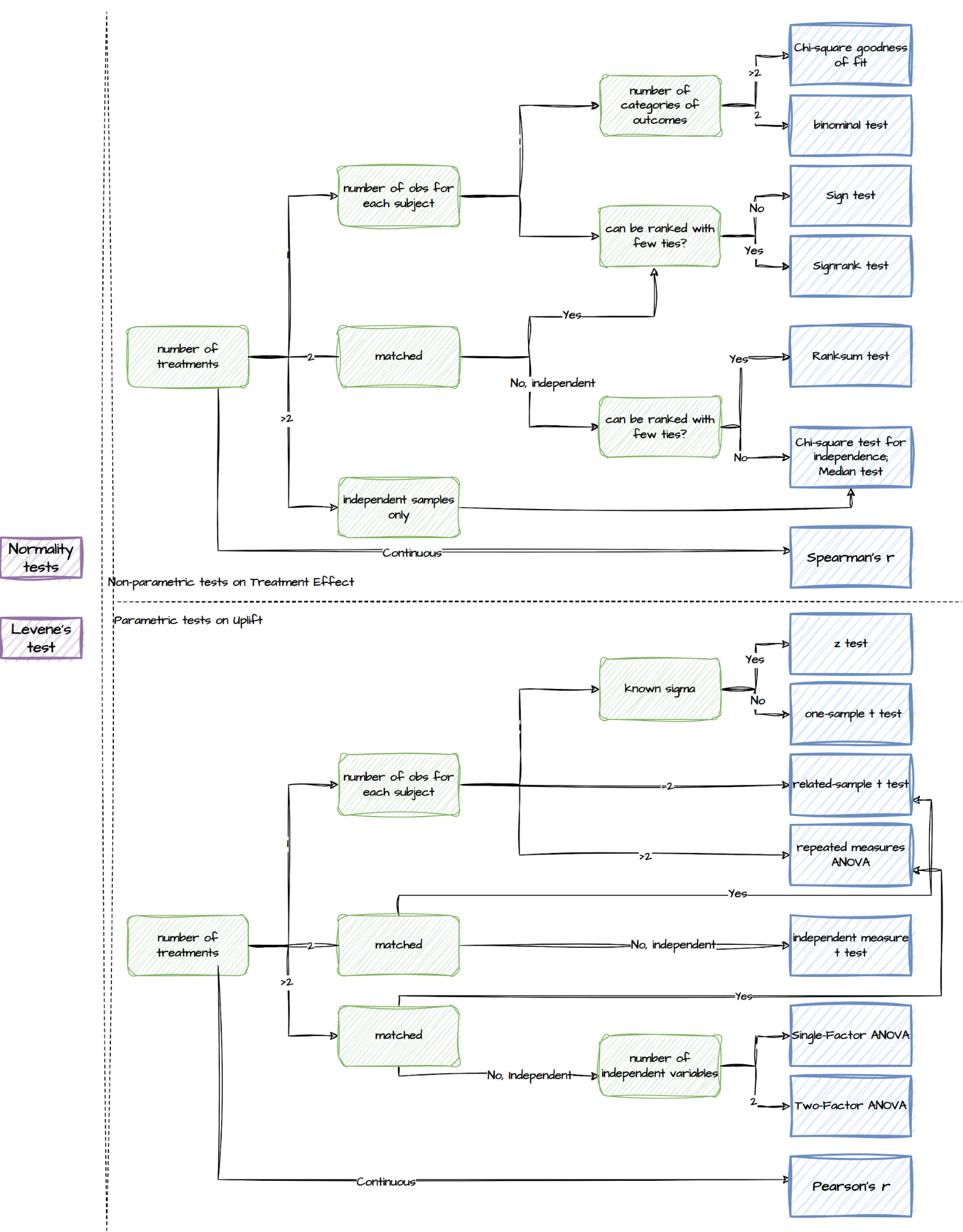
Though we make all the relevant tests available, the package sets a default list of output. With just two lines of code specifying the desired experiment design, experimenters can easily retrieve the recommended results, as summarised in the following table.

Types Details
Basic statistics The mean, variance, and sample size of Treatment and Control
Uplift tests Welch’s t-test;
Non-parametric tests, such as Wilcoxon signed-rank test and Mann-Whitney U Test
Misc tests Normality tests such as the Shapiro-Wilk test, Anderson-Darling test, and Kolmogorov-Smirnov test;
Levene test which assesses the equality of variances between groups
Regression models A standard OLS/Logit model to estimate the treatment uplift;
Recommended regression models
Warning Provides a warning or notification related to the statistical analysis or results, for example:
– Lack of variation in the variables
– Sample size is too small
– Too few randomisation units which will lead to under-estimated standard errors

Besides reporting relevant statistical test results, we adopt regression models to leverage their flexibility in controlling for confounders, fixed effects and heteroskedasticity, as is commonly observed in our experiments. As mentioned in the section “A note on experimental design”, each approach has different implications on the achieved randomisation, and hence requires its own customised regression models.

Between-subject design: the observations are not independent and identically distributed (i.i.d) but clustered due to repeated observations of the same experimental units. Therefore, we set the default clustering level at the participant level in our regression models, considering that most of our between-subject experiments only take a small portion of the population (Abadie et al., 2022).

Within-subject design: this has further challenges, including spillover effects and randomisation imbalances. As a result, they often require better control of confounding factors. We adopt panel data methods and impose time fixed effects, with no option to remove them. Though users have the flexibility to define these themselves, we use hourly fixed effects as our default as we have found that these match the typical seasonality we observe in marketplace metrics. Similar to between-subject
designs, we use standard error corrections for clustered errors, and small number of clusters, as the default. Our API is flexible for users to include further controls, as well as further fixed effects to adapt the estimator to geo-timeslice designs.

Advanced tools

Apart from the pre-experiment Trusted Advisor and the post-experiment Analysis Toolbox, we have enriched this package by providing more advanced tools. Some of them are set as a default feature in the previous two components, while others are ad-hoc capabilities which the users can utilise via calling the functions directly.

Variance reduction

We bring in multiple methods to reduce variance and improve the power and sensitivity of experiments:

  • Stratified sampling: recognised for reducing variance during assignment
  • Post stratification: a post-assignment variance reduction technique
  • CUPED: utilises ANCOVA to decrease variances
  • MLRATE: an extension of CUPED that allows for the use of non-linear / machine learning models

These approaches offer valuable ways to mitigate variance and improve the overall effectiveness of experiments. The experimenters can directly access these ad hoc capabilities via the package.

Multiple comparisons problem

A multiple comparisons problem occurs when multiple hypotheses are simultaneously tested, leading to a higher likelihood of false positives. To address this, we implement various statistical correction techniques in this package, as illustrated below.

Statistical correction techniques

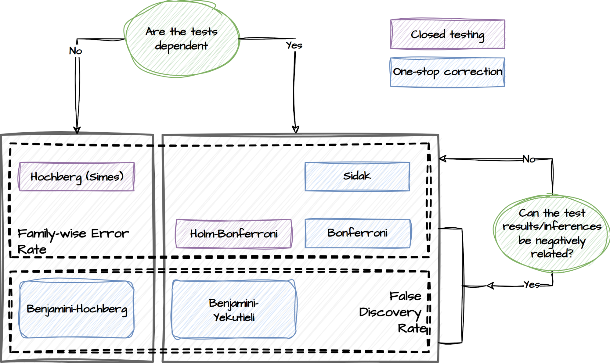
Experimenters can specify if they have concerns about the dependency of the tests and whether the test results are expected to be negatively related. This capability will adopt the following procedures and choose the relevant tests to mitigate the risk of false positives accordingly:

  • False Discovery Rate (FDR) procedures, which control the expected rate of false discoveries.
  • Family-wise Error Rate (FWER) procedures, which control the probability of making at least one false discovery within a set of related tests referred to as a family.

Multiple treatments and unequal treatment sizes

We developed a capability to deal with experiments where there are multiple treatments. This capability employs a conservative approach to ensure that the size reaches a minimum level where any pairwise comparison between the control and treatment groups has a sufficient sample size.

Heterogeneous treatment effects

Heterogeneous treatment effects refer to a situation where the treatment effect varies across different groups or subpopulations within a larger population. For instance, it may be of interest to examine treatment effects specifically on rainy days compared to non-rainy days. We have incorporated this functionality into the tests for both experiment designs. By enabling this feature, we facilitate a more nuanced analysis that accounts for potential variations in treatment effects based on different factors or contexts.

Maintenance and support

The package is available across all internal DS/Machine Learning platforms and individual local development environments within Grab. Its source code is openly accessible to all developers within Grab and its release adheres to a semantic release standard.

In addition to the technical maintenance efforts, we have introduced a dedicated committee and a workspace to address issues that may extend beyond the scope of the package’s current capabilities.

Experiment Council

Within Grab, there is a dedicated committee known as the ‘Experiment Council’. This committee includes data scientists, analysts, and economists from various functions. One of their responsibilities is to collaborate to enhance and maintain the package, as well as guide users in effectively utilising its functionalities. The Experiment Council plays a crucial role in enhancing the overall operational excellence of conducting experiments and deriving meaningful insights from them.

GrabCausal Methodology Bank

Experimenters frequently encounter challenges regarding the feasibility of conducting experiments for causal problems. To address this concern, we have introduced an alternative workspace called GrabCausal Methodology Bank. Similar to the internal open-source nature of this project, the GrabCausal Methodology bank is open to contributions from all users within Grab. It provides a collaborative space where users can readily share their code, case studies, guidelines, and suggestions related to
causal methodologies. By fostering an open and inclusive environment, this workspace encourages knowledge sharing and promotes the advancement of causal research methods.

The workspace functions as a platform, which now exhibits a wide range of commonly used methods, including Diff-in-Diff, Event studies, Regression Discontinuity Designs (RDD), Instrumental Variables (IV), Bayesian structural time series, and Bunching. Additionally, we are dedicated to incorporating more, such as Synthetic control, Double ML (Chernozhukov et al. 2018), DAG discovery/validation, etc., to further enhance our offerings in this space.

Learnings

Over the past few years, we have invested in developing and expanding this package. Our initial motivation was humble yet motivating – to contribute to improving the quality of experimentation at Grab, helping it develop from its initial start-up modus operandi to a more consolidated, rigorous, and guided approach.

Throughout this journey, we have learned that prioritisation holds the utmost significance in open-source projects of this nature; the majority of user demands can be met through relatively small yet pivotal efforts. By focusing on these core capabilities, we avoid spreading resources too thinly across all areas at the initial stage of planning and development.

Meanwhile, we acknowledge that there is still a significant journey ahead. While the package now focuses solely on individual experiments, an inherent challenge in online-controlled experimentation platforms is the interference between experiments (Gupta, et al, 2019). A recent development in the field is to embrace simultaneous tests (Microsoft, Google, Spotify and booking.com and Optimizely), and to carefully consider the tradeoff between accuracy and velocity.

The key to overcoming this challenge will be a close collaboration between the community of experimenters, the teams developing this unified toolkit, and the GrabX platform engineers. In particular, the platform developers will continue to enrich the experimentation SDK by providing diverse assignment strategies, sampling mechanisms, and user interfaces to manage potential inference risks better. Simultaneously, the community of experimenters can coordinate among themselves effectively to
avoid severe interference, which will also be monitored by GrabX. Last but not least, the development of this unified toolkit will also focus on monitoring, evaluating, and managing inter-experiment interference.

In addition, we are committed to keeping this package in sync with industry advancements. Many existing tools in this package, despite being labelled as “advanced” in the earlier discussions, are still relatively simplified. For instance,

  • Incorporating standard errors clustering based on the diverse assignment and sampling strategies requires attention (Abadie, et al, 2023).
  • Sequential testing will play a vital role in detecting uplifts earlier and safely, avoiding p-hacking. One recent innovation is the “always valid inference” (Johari, et al., 2022)
  • The advancements in investigating heterogeneous effects, such as Causal Forest (Athey and Wager, 2019), have extended beyond linear approaches, now incorporating nonlinear and more granular analyses.
  • Estimating the long-term treatment effects observed from short-term follow-ups is also a long-term objective, and one approach is using a Surrogate Index (Athey, et al 2019).
  • Continuous effort is required to stay updated and informed about the latest advancements in statistical testing methodologies, to ensure accuracy and effectiveness.

This article marks the beginning of our journey towards automating the experimentation and product decision-making process among the data scientist community. We are excited about the prospect of expanding the toolkit further in these directions. Stay tuned for more updates and posts.

References

  • Abadie, Alberto, et al. “When should you adjust standard errors for clustering?.” The Quarterly Journal of Economics 138.1 (2023): 1-35.

  • Athey, Susan, et al. “The surrogate index: Combining short-term proxies to estimate long-term treatment effects more rapidly and precisely.” No. w26463. National Bureau of Economic Research, 2019.

  • Athey, Susan, and Stefan Wager. “Estimating treatment effects with causal forests: An application.” Observational studies 5.2 (2019): 37-51.

  • Chernozhukov, Victor, et al. “Double/debiased machine learning for treatment and structural parameters.” (2018): C1-C68.

  • Facure, Matheus. Causal Inference in Python. O’Reilly Media, Inc., 2023.

  • Gupta, Somit, et al. “Top challenges from the first practical online controlled experiments summit.” ACM SIGKDD Explorations Newsletter 21.1 (2019): 20-35.

  • Huntington-Klein, Nick. The Effect: An Introduction to Research Design and Causality. CRC Press, 2021.

  • Imbens, Guido W. and Donald B. Rubin. Causal Inference for Statistics, Social, and Biomedical Sciences: An Introduction. Cambridge University Press, 2015.

  • Johari, Ramesh, et al. “Always valid inference: Continuous monitoring of a/b tests.” Operations Research 70.3 (2022): 1806-1821.

  • List, John A., Sally Sadoff, and Mathis Wagner. “So you want to run an experiment, now what? Some simple rules of thumb for optimal experimental design.” Experimental Economics 14 (2011): 439-457.

  • Moffatt, Peter. Experimetrics: Econometrics for Experimental Economics. Bloomsbury Publishing, 2020.

Join us

Grab is the leading superapp platform in Southeast Asia, providing everyday services that matter to consumers. More than just a ride-hailing and food delivery app, Grab offers a wide range of on-demand services in the region, including mobility, food, package and grocery delivery services, mobile payments, and financial services across 428 cities in eight countries.

Powered by technology and driven by heart, our mission is to drive Southeast Asia forward by creating economic empowerment for everyone. If this mission speaks to you, join our team today!

Total eclipse of the Internet: Traffic impacts in Mexico, the US, and Canada

Post Syndicated from João Tomé original https://blog.cloudflare.com/total-eclipse-internet-traffic-impacts-mexico-us-canada


A photo of the eclipse taken by Bryton Herdes, a member of our Network team, in Southern Illinois.

There are events that unite people, like a total solar eclipse, reminding us, humans living on planet Earth, of our shared dependence on the sun. Excitement was obvious in Mexico, several US states, and Canada during the total solar eclipse that occurred on April 8, 2024. Dubbed the Great North American Eclipse, millions gathered outdoors to witness the Moon pass between Earth and the Sun, casting darkness over fortunate states. Amidst the typical gesture of putting the eclipse glasses on and taking them off, depending on if people were looking at the sky during the total eclipse, or before or after, what happened to Internet traffic?

Cloudflare’s data shows a clear impact on Internet traffic from Mexico to Canada, following the path of totality. The eclipse occurred between 15:42 UTC and 20:52 UTC, moving from south to north, as seen in this NASA image of the path and percentage of darkness of the eclipse.

Looking at the United States in aggregate terms, bytes delivered traffic dropped by 8%, and request traffic by 12% as compared to the previous week at 19:00 UTC (14:00 Eastern, 12:00 Pacific).

Bytes delivered percentage change (-8% at 19:00 UTC)

HTTP requests percentage change (-12% at 19:00 UTC)

The state-level perspective in terms of traffic drop at the time of the eclipse, as compared to the previous week, is much more revealing. Here’s a summary of the US states’ traffic changes. We can almost trace the path of the eclipse, as shown in the previous NASA image.

From our data, Vermont, Arkansas, Indiana, Maine, New Hampshire, and Ohio experienced traffic drops of 40% or more around the time of the eclipse. These states were all in the path of totality, which was not the case for several others.

In the next table, we provide a detailed breakdown of the same perspective shown on the US map ordered by drop in traffic. In all of these charts, we’re using UTC as the time. We include the time of the biggest traffic drop compared to the previous week, at a 5-minute granularity, and also the percentage of drop compared to the previous week. States where it was possible to see at least part of the total eclipse are highlighted in bold. At the bottom are those with no clear difference.

The US: traffic change at time of the eclipse

State

Time of drop (UTC)

Local time

% of drop

Vermont

19:25

15:25

-60%

Arkansas

18:50

13:50

-54%

Indiana

19:05

15:05

-50%

Maine

19:30

15:30

-48%

New Hampshire

19:20

15:20

-40%

Ohio

19:10

15:10

-40%

Kentucky

19:05

14:05

-33%

Massachusetts

19:25

15:25

-33%

Michigan

19:15

15:15

-32%

Kansas

18:50

13:50

-31%

Missouri

18:55

13:55

-31%

Connecticut

19:20

15:20

-29%

Maryland

19:15

15:15

-29%

New York

19:25

15:25

-29%

Oklahoma

18:45

13:45

-29%

Rhode Island

19:25

15:25

-29%

New Jersey

19:20

15:20

-28%

Arizona

18:15

11:15

-27%

Illinois

19:05

14:05

-26%

Pennsylvania

19:15

15:15

-26%

West Virginia

19:15

15:15

-24%

Wisconsin

19:05

14:05

-22%

Wyoming

18:20

12:20

-19%

Alaska

20:15

12:15

-18%

Delaware

19:20

15:20

-18%

District of Columbia

19:15

15:15

-16%

New Mexico

18:25

12:25

-16%

Oregon

18:15

11:15

-16%

Nebraska

18:50

13:50/12:50

-15%

Texas

18:45

13:45

-15%

Colorado

18:25

12:25

-14%

Virginia

18:20

14:20

-14%

Alabama

19:00

14:00

-13%

Tennessee

19:00

15:00/14:00

-13%

Iowa

18:15

13:15

-12%

Nevada

18:10

11:10

-12%

Georgia

19:05

15:05

-11%

North Carolina

19:10

15:10

-10%

California

18:15

11:15

-9%

Florida

18:15

14:15

-7%

Utah

18:15

12:15

-5%

Montana

18:25

12:25

-4%

South Carolina

19:00

15:00

-4%

Hawaii

Louisiana

Minnesota

Mississippi

North Dakota

Idaho

South Dakota

Washington

Visualized, here’s what Vermont’s 60% drop looks like:

And here’s what the traffic drops in Arkansas, Maine, and Indiana look like:

In terms of states with larger populations, New York took the lead:

Mexico got the eclipse first

Before the eclipse became visible in the US, Mexico experienced it first. States within the eclipse zone, such as Coahuila, Durango, and Sinaloa, experienced noticeable drops in traffic. Even Mexico City, located further south, was affected.

Mexico: traffic change at time of the eclipse

State

Time of drop (UTC)

Local time

% of drop

Durango

18:15

12:15

-57%

Coahuila

18:15

12:15

-43%

Sinaloa

18:10

11:10

-34%

Mexico City

18:10

12:10

-22%

Here’s the Durango and Coahuila state perspectives:

Canada at last: an island stopped to see the eclipse

After Mexico and the US, Canada was next in the path of the eclipse. Prince Edward Island experienced the most significant impact in Canada. This region, with a population of less than 200,000, is one of eastern Canada’s maritime provinces, situated off New Brunswick and Nova Scotia in the Gulf of St. Lawrence. Next came New Brunswick and Newfoundland and Labrador.

Canada: traffic change at time of the eclipse

State

Time of drop (UTC)

Local time

% of drop

Prince Edward Island

19:35

16:35

-48%

New Brunswick

19:30

16:30

-40%

Newfoundland and Labrador

19:40

16:10

-32%

Nova Scotia

19:35

16:35

-27%

Quebec

19:25

15:25

-27%

Ontario

19:15

15:15

-21%

Conclusion: Internet is a human’s game

As we’ve observed during previous occasions, human and nature-related events significantly impact Internet traffic. This includes Black Friday/Cyber Week, Easter, Ramadan celebrations, the coronation of King Charles II, the recent undersea cable failure in Africa, which affected 13 countries, and now, this total eclipse.

This was the last total solar eclipse visible in the contiguous United States until August 23, 2044, with the next eclipse of similar breadth projected for August 12, 2045.

For this and other trends, visit Cloudflare Radar and follow us on social media at @CloudflareRadar (X), cloudflare.social/@radar (Mastodon), and radar.cloudflare.com (Bluesky).

Amazon DataZone announces integration with AWS Lake Formation hybrid access mode for the AWS Glue Data Catalog

Post Syndicated from Utkarsh Mittal original https://aws.amazon.com/blogs/big-data/amazon-datazone-announces-integration-with-aws-lake-formation-hybrid-access-mode-for-the-aws-glue-data-catalog/

Last week, we announced the general availability of the integration between Amazon DataZone and AWS Lake Formation hybrid access mode. In this post, we share how this new feature helps you simplify the way you use Amazon DataZone to enable secure and governed sharing of your data in the AWS Glue Data Catalog. We also delve into how data producers can share their AWS Glue tables through Amazon DataZone without needing to register them in Lake Formation first.

Overview of the Amazon DataZone integration with Lake Formation hybrid access mode

Amazon DataZone is a fully managed data management service to catalog, discover, analyze, share, and govern data between data producers and consumers in your organization. With Amazon DataZone, data producers populate the business data catalog with data assets from data sources such as the AWS Glue Data Catalog and Amazon Redshift. They also enrich their assets with business context to make it straightforward for data consumers to understand. After the data is available in the catalog, data consumers such as analysts and data scientists can search and access this data by requesting subscriptions. When the request is approved, Amazon DataZone can automatically provision access to the data by managing permissions in Lake Formation or Amazon Redshift so that the data consumer can start querying the data using tools such as Amazon Athena or Amazon Redshift.

To manage the access to data in the AWS Glue Data Catalog, Amazon DataZone uses Lake Formation. Previously, if you wanted to use Amazon DataZone for managing access to your data in the AWS Glue Data Catalog, you had to onboard your data to Lake Formation first. Now, the integration of Amazon DataZone and Lake Formation hybrid access mode simplifies how you can get started with your Amazon DataZone journey by removing the need to onboard your data to Lake Formation first.

Lake Formation hybrid access mode allows you to start managing permissions on your AWS Glue databases and tables through Lake Formation, while continuing to maintain any existing AWS Identity and Access Management (IAM) permissions on these tables and databases. Lake Formation hybrid access mode supports two permission pathways to the same Data Catalog databases and tables:

  • In the first pathway, Lake Formation allows you to select specific principals (opt-in principals) and grant them Lake Formation permissions to access databases and tables by opting in
  • The second pathway allows all other principals (that are not added as opt-in principals) to access these resources through the IAM principal policies for Amazon Simple Storage Service (Amazon S3) and AWS Glue actions

With the integration between Amazon DataZone and Lake Formation hybrid access mode, if you have tables in the AWS Glue Data Catalog that are managed through IAM-based policies, you can publish these tables directly to Amazon DataZone, without registering them in Lake Formation. Amazon DataZone registers the location of these tables in Lake Formation using hybrid access mode, which allows managing permissions on AWS Glue tables through Lake Formation, while continuing to maintain any existing IAM permissions.

Amazon DataZone enables you to publish any type of asset in the business data catalog. For some of these assets, Amazon DataZone can automatically manage access grants. These assets are called managed assets, and include Lake Formation-managed Data Catalog tables and Amazon Redshift tables and views. Prior to this integration, you had to complete the following steps before Amazon DataZone could treat the published Data Catalog table as a managed asset:

  1. Identity the Amazon S3 location associated with Data Catalog table.
  2. Register the Amazon S3 location with Lake Formation in hybrid access mode using a role with appropriate permissions.
  3. Publish the table metadata to the Amazon DataZone business data catalog.

The following diagram illustrates this workflow.

With the Amazon DataZone’s integration with Lake Formation hybrid access mode, you can simply publish your AWS Glue tables to Amazon DataZone without having to worry about registering the Amazon S3 location or adding an opt-in principal in Lake Formation by delegating these steps to Amazon DataZone. The administrator of an AWS account can enable the data location registration setting under the DefaultDataLake blueprint on the Amazon DataZone console. Now, a data owner or publisher can publish their AWS Glue table (managed through IAM permissions) to Amazon DataZone without the extra setup steps. When a data consumer subscribes to this table, Amazon DataZone registers the Amazon S3 locations of the table in hybrid access mode, adds the data consumer’s IAM role as an opt-in principal, and grants access to the same IAM role by managing permissions on the table through Lake Formation. This makes sure that IAM permissions on the table can coexist with newly granted Lake Formation permissions, without disrupting any existing workflows. The following diagram illustrates this workflow.

Solution overview

To demonstrate this new capability, we use a sample customer scenario where the finance team wants to access data owned by the sales team for financial analysis and reporting. The sales team has a pipeline that creates a dataset containing valuable information about ticket sales, popular events, venues, and seasons. We call it the tickit dataset. The sales team stores this dataset in Amazon S3 and registers it in a database in the Data Catalog. The access to this table is currently managed through IAM-based permissions. However, the sales team wants to publish this table to Amazon DataZone to facilitate secure and governed data sharing with the finance team.

The steps to configure this solution are as follows:

  1. The Amazon DataZone administrator enables the data lake location registration setting in Amazon DataZone to automatically register the Amazon S3 location of the AWS Glue tables in Lake Formation hybrid access mode.
  2. After the hybrid access mode integration is enabled in Amazon DataZone, the finance team requests a subscription to the sales data asset. The asset shows up as a managed asset, which means Amazon DataZone can manage access to this asset even if the Amazon S3 location of this asset isn’t registered in Lake Formation.
  3. The sales team is notified of a subscription request raised by the finance team. They review and approve the access request. After the request is approved, Amazon DataZone fulfills the subscription request by managing permissions in the Lake Formation. It registers the Amazon S3 location of the subscribed table in Lake Formation hybrid mode.
  4. The finance team gains access to the sales dataset required for their financial reports. They can go to their DataZone environment and start running queries using Athena against their subscribed dataset.

Prerequisites

To follow the steps in this post, you need an AWS account. If you don’t have an account, you can create one. In addition, you must have the following resources configured in your account:

  • An S3 bucket
  • An AWS Glue database and crawler
  • IAM roles for different personas and services
  • An Amazon DataZone domain and project
  • An Amazon DataZone environment profile and environment
  • An Amazon DataZone data source

If you don’t have these resources already configured, you can create them by deploying the following AWS CloudFormation stack:

  1. Choose Launch Stack to deploy a CloudFormation template.
  2. Complete the steps to deploy the template and leave all settings as default.
  3. Select I acknowledge that AWS CloudFormation might create IAM resources, then choose Submit.

After the CloudFormation deployment is complete, you can log in to the Amazon DataZone portal and manually trigger a data source run. This pulls any new or modified metadata from the source and updates the associated assets in the inventory. This data source has been configured to automatically publish the data assets to the catalog.

  1. On the Amazon DataZone console, choose View domains.

You should be logged in using the same role that is used to deploy CloudFormation and verify that you are in the same AWS Region.

  1. Find the domain blog_dz_domain, then choose Open data portal.
  2. Choose Browse all projects and choose Sales producer project.
  3. On the Data tab, choose Data sources in the navigation pane.
  4. Locate and choose the data source that you want to run.

This opens the data source details page.

  1. Choose the options menu (three vertical dots) next to tickit_datasource and choose Run.

The data source status changes to Running as Amazon DataZone updates the asset metadata.

Enable hybrid mode integration in Amazon DataZone

In this step, the Amazon DataZone administrator goes through the process of enabling the Amazon DataZone integration with Lake Formation hybrid access mode. Complete the following steps:

  1. On a separate browser tab, open the Amazon DataZone console.

Verify that you are in the same Region where you deployed the CloudFormation template.

  1. Choose View domains.
  2. Choose the domain created by AWS CloudFormation, blog_dz_domain.
  3. Scroll down on the domain details page and choose the Blueprints tab.

A blueprint defines what AWS tools and services can be used with the data assets published in Amazon DataZone. The DefaultDataLake blueprint is enabled as part of the CloudFormation stack deployment. This blueprint enables you to create and query AWS Glue tables using Athena. For the steps to enable this in your own deployments, refer to Enable built-in blueprints in the AWS account that owns the Amazon DataZone domain.

  1. Choose the DefaultDataLake blueprint.
  2. On the Provisioning tab, choose Edit.
  3. Select Enable Amazon DataZone to register S3 locations using AWS Lake Formation hybrid access mode.

You have the option of excluding specific Amazon S3 locations if you don’t want Amazon DataZone to automatically register them to Lake Formation hybrid access mode.

  1. Choose Save changes.

Request access

In this step, you log in to Amazon DataZone as the finance team, search for the sales data asset, and subscribe to it. Complete the following steps:

  1. Return to your Amazon DataZone data portal browser tab.
  2. Switch to the finance consumer project by choosing the dropdown menu next to the project name and choosing Finance consumer project.

From this step onwards, you take on the persona of a finance user looking to subscribe to a data asset published in the previous step.

  1. In the search bar, search for and choose the sales data asset.
  2. Choose Subscribe.

The asset shows up as managed asset. This means that Amazon DataZone can grant access to this data asset to the finance team’s project by managing the permissions in Lake Formation.

  1. Enter a reason for the access request and choose Subscribe.

Approve access request

The sales team gets a notification that an access request from the finance team is submitted. To approve the request, complete the following steps:

  1. Choose the dropdown menu next to the project name and choose Sales producer project.

You now assume the persona of the sales team, who are the owners and stewards of the sales data assets.

  1. Choose the notification icon at the top-right corner of the DataZone portal.
  2. Choose the Subscription Request Created task.
  3. Grant access to the sales data asset to the finance team and choose Approve.

Analyze the data

The finance team has now been granted access to the sales data, and this dataset has been to their Amazon DataZone environment. They can access the environment and query the sales dataset with Athena, along with any other datasets they currently own. Complete the following steps:

  1. On the dropdown menu, choose Finance consumer project.

On the right pane of the project overview screen, you can find a list of active environments available for use.

  1. Choose the Amazon DataZone environment finance_dz_environment.
  2. In the navigation pane, under Data assets, choose Subscribed.
  3. Verify that your environment now has access to the sales data.

It may take a few minutes for the data asset to be automatically added to your environment.

  1. Choose the new tab icon for Query data.

A new tab opens with the Athena query editor.

  1. For Database, choose finance_consumer_db_tickitdb-<suffix>.

This database will contain your subscribed data assets.

  1. Generate a preview of the sales table by choosing the options menu (three vertical dots) and choosing Preview table.

Clean up

To clean up your resources, complete the following steps:

  1. Switch back to the administrator role you used to deploy the CloudFormation stack.
  2. On the Amazon DataZone console, delete the projects used in this post. This will delete most project-related objects like data assets and environments.
  3. On the AWS CloudFormation console, delete the stack you deployed in the beginning of this post.
  4. On the Amazon S3 console, delete the S3 buckets containing the tickit dataset.
  5. On the Lake Formation console, delete the Lake Formation admins registered by Amazon DataZone.
  6. On the Lake Formation console, delete tables and databases created by Amazon DataZone.

Conclusion

In this post, we discussed how the integration between Amazon DataZone and Lake Formation hybrid access mode simplifies the process to start using Amazon DataZone for end-to-end governance of your data in the AWS Glue Data Catalog. This integration helps you bypass the manual steps of onboarding to Lake Formation before you can start using Amazon DataZone.

For more information on how to get started with Amazon DataZone, refer to the Getting started guide. Check out the YouTube playlist for some of the latest demos of Amazon DataZone and short descriptions of the capabilities available. For more information about Amazon DataZone, see How Amazon DataZone helps customers find value in oceans of data.


About the Authors

Utkarsh Mittal is a Senior Technical Product Manager for Amazon DataZone at AWS. He is passionate about building innovative products that simplify customers’ end-to-end analytics journeys. Outside of the tech world, Utkarsh loves to play music, with drums being his latest endeavor.

Praveen Kumar is a Principal Analytics Solution Architect at AWS with expertise in designing, building, and implementing modern data and analytics platforms using cloud-centered services. His areas of interests are serverless technology, modern cloud data warehouses, streaming, and generative AI applications.

Paul Villena is a Senior Analytics Solutions Architect in AWS with expertise in building modern data and analytics solutions to drive business value. He works with customers to help them harness the power of the cloud. His areas of interests are infrastructure as code, serverless technologies, and coding in Python

How to Send SMS Using a Sender ID with Amazon Pinpoint

Post Syndicated from Tyler Holmes original https://aws.amazon.com/blogs/messaging-and-targeting/how-to-send-sms-using-a-sender-id-with-amazon-pinpoint/

Amazon Pinpoint enables you to send text messages (SMS) to recipients in over 240 regions and countries around the world. Pinpoint supports all types of origination identities including Long Codes, 10DLC (US only), Toll-Free (US only), Short Codes, and Sender IDs.
NOTE: Certain subtypes of Origination Identities (OIDs), such as Free to End User (FTEU) Short Codes might not be supported

Unlike other origination identities, a Sender ID can include letters, enabling your recipients to receive SMS from “EXAMPLECO” rather than a random string of numbers or phone number. A Sender ID can help to create trust and brand awareness with your recipients which can increase your deliverability and conversion rates by improving customer interaction with your messages. In this blog we will discuss countries that allow the use of Sender IDs, the types of Sender IDs that Pinpoint supports, how to configure Pinpoint to use a Sender ID, and best practices for sending SMS with a Sender ID. Refer to this blog post for guidance planning a multi-country rollout of SMS.

What is a Sender ID?

A sender ID is an alphanumeric name that identifies the sender of an SMS message. When you send an SMS message using a sender ID, and the recipient is in an area where sender ID is supported, your sender ID appears on the recipient’s device instead of a phone number, for example, they will see AMAZON instead of a phone number such as “1-206-555-1234”. Sender IDs support a default throughput of 10 messages per second (MPS), which can be raised in certain situations. This MPS is calculated at the country level. As an example, a customer can send 10 MPS with “SENDERX” to Australia (AU) and 10 MPS with “SENDERX” to Germany (DE).

The first step in deciding whether to use a Sender ID is finding out whether the use of a Sender ID is supported by the country(ies) you want to send to. This table lists all of the destinations that Pinpoint can send SMS to and the Origination Identities that they support. Many countries support multiple origination identities so it’s important to know the differences between them. The two main considerations when deciding what originator to use is throughput and whether it can support a two-way use case.

Amazon Pinpoint supports three types of Sender IDs detailed below. Your selection is dependent on the destination country for your messages, consult this table that lists all of the destinations that Pinpoint can send SMS to.

Dynamic Sender ID – A dynamic sender ID allows you to select a 3-11 character alphanumeric string to use as your originator when sending SMS. We suggest using something short that outlines your brand and use case like “[Company]OTP.” Dynamic sender IDs vary slightly by country and we recommended senders review the specific requirements for the countries they plan to send to. Pay special attention to any notes in the registration section. If the country(ies) you want to send to require registration, read on to the next type of Sender ID.

Registered Sender ID – A registered SenderID generally follows the same formatting requirements as a Dynamic Sender ID, alowing you to select a 3-11 character alphanumeric string to use, but has the added step of completing a registration specific to the country you want to use a Sender ID for. Each country will require slightly different information to register, may require specific forms, as well as a potential registration fee. Use this list of supported countries to see what countries support Sender ID as well as which ones require registration.

Generic, or “Shared” Sender ID – In countries where it is supported, when you do not specify a dynamic Sender ID, or you have not set a Default Sender ID in Pinpoint, the service may allow traffic over a Generic or Shared SenderID like NOTICE. Depending on the country, traffic could also be delivered using a service or carrier specific long or short code. When using the shared route your messages will be delivered alongside others also sending in this manner.

As mentioned, Sender IDs support 10 MPS, so if you do not need higher throughput than this may be a good option. However, one of the key differences of using a Sender ID to send SMS is that they do not support two-way use cases, meaning they cannot receive SMS back from your recipients.

IMPORTANT: If you use a sender ID you must provide your recipients with alternative ways to opt-out of your communications as they cannot text back any of the standard opt-out keywords or any custom opt-in keywords you may have configured. Common ways to offer your recipients an alternative way of opting out or changing their communication preferences include web forms or an app preference center.

How to Configure a Sender ID

The country(ies) you plan on sending to using a Sender ID will determine the configuration you will need to complete to be able to use them. We will walk through the configuration of each of the three types of Sender IDs below.

Step 1 – Request a Sender ID(Dependent on Country, Consult this List)

Some countries require a registration process. Each process, dependent on the country can be unique so it is required that a case be opened to complete this process. The countries requiring Sender ID registration are noted in the following list.
When you request a Sender ID, we provide you with an estimate of how long the request will take to complete. This estimate is based on the completion times that we’ve seen from other customers.

NOTE: This time is not an SLA. It is recommended that you check the case regularly and make sure that nothing else is required to complete your registration. If your registration requires edits it will extend this process each time it requires edits. If your registration passes over the estimated time it is recommended that you reply to the case.

Because each country has its own process, completion times for registration vary by destination country. For example, Sender ID registration in India can be completed in one week or less, whereas it can take six weeks or more in Vietnam. These requests can’t be expedited, because they involve the carriers themselves making changes to the ways that their networks are configured and certify the use case onto their network. We suggest that you start your registration process early so that you can start sending messages as soon as you launch your product or service.

IMPORTANT: Make sure that you are checking on your case often as support may need more details to complete your registration and any delay extends the expected timeline for procuring your Sender ID

Generic Sender ID – In countries that support a Generic or Shared ID like NOTICE there is no requirement to register or configure prior to sending we will review how to send with this type of Sender ID in Step 2.

Dynamic Sender ID – A Dynamic Sender ID can be requested via the API or in the console, complete the following steps to configure these Sender IDs in the console.
NOTE: If you are using the API to send it is not required that you request a Sender ID for every country that you intend on sending to. However, it is recommended, because the request process will alert you to any Sender IDs that require registration so you do not attempt to send to countries that you cannot deliver successfully to. All countries requiring registration for Sender IDs can be found here.

  1. Navigate to the SMS Console
    1. Make sure you are in the region you plan on using to send SMS out of as each region needs to be configured independently and any registrations also need to be made in the account and region in which you will be sending from
  2. Select “Sender IDs” from the left rail
    1. Click on “Request Originator”
    2. Choose a country from the drop down that supports Sender ID
    3. Choose “SMS”
      1. Leave “Voice” unchecked if it is an option.
        NOTE: If you choose Voice than you will not be able to select a Sender ID in the next step
      2. Select your estimated SMS volume
      3. Choose whether your company is local or international in relation to the country you are wanting to configure. Some countries, like India, require proof of residency to access local pricing so select accordingly.
      4. Select “No” for two-way messaging or you will not be able to select a Sender ID in the next step
    4. Click next and choose “Sender ID” and provide your preferred Sender ID.
      NOTE: Refer to the following criteria when selecting your Sender ID for configuration (some countries may override these)

      1. Numeric-only Sender IDs are not supported
      2. No special characters except for dashes ( – )
      3. No spaces
      4. Valid characters: a-z, A-Z, 0-9
      5. Minimum of 3 characters
      6. Maximum of 11 characters. NOTE: India is exactly 6 Characters
      7. Must match your company branding and SMS service or use case.
        1. For example, you wouldn’t be able to choose “OTP” or “2FA” even though you might be using SMS for that type of a use case. You could however use “ANYCO-OTP” if your company name was “Any Co.” since it complies with all above criteria.


NOTE: If the console instructs you to open a case as seen below than your Sender ID likely requires some form of registration. Read on to configure a Registered Sender ID.

Registered Sender ID – A registered sender ID follows the same criteria above for a Dynamic Sender ID, although some countries may have minor criteria changes or formatting restrictions. Follow the directions here to complete this process, AWS support will provide the correct forms needed for the country that you are registering. Each Registered Sender ID will need a separate case per country. Follow the link to the “AWS Support Center” and follow these instructions when creating your case

Step 2 – How to Send SMS with a Sender ID

Sender IDs can be used via three different mechanisms

Option 1 – Using the V2 SMS and Voice API and “SendTextMessage
This is the preferred method of sending and this set of APIs is where all new functionality will be built on.

  1. SendTextMessage has many options for configurability but the only required parameters are the following:
    1. DestinationPhoneNumber
    2. MessageBody
  2. “OriginationIdentity” is optional, but it’s important to know what the outcome is dependent on how you use this parameter:
    1. Explicitly stating your SenderId
      1. Use this option if you want to ONLY send with a Sender ID. Setting this has the effect of only sending to recipients in countries that accept SenderIDs and rejecting any recipients whose country does not support Sender IDs. The US for example cannot be sent to with a Sender ID
    2. Explicitly stating your SenderIdArn
      1. Same effect as “SenderID” above
    3. Leaving OriginationIdentity Blank
      1. If left blank Pinpoint will select the right originator based on what you have available in your account in order of decreasing throughput, from a Short Code, 10DLC (US Only), Long Code, Sender ID, or Toll-Free (US Only), depending on what you have available.
        1. Keep in mind that sending this way opens you up to sending to countries you may not have originators for. If you would like to make sure that you are only sending to countries that you have originators for then you need to use Pools.
    4. Explicitly stating a PoolId
      1. A pool is a collection of Origination Identities that can include both phone numbers and Sender IDs. Use this option if you are sending to multiple country codes and want to make sure that you send to them with the originator that their respective country supports.
        1. NOTE: There are various configurations that can be set on a pool. Refer to the documentation here
          1. Make sure to pay particular attention to “Shared Routes” because in some countries, Amazon Pinpoint SMS maintains a pool of shared origination identities. When you activate shared routes, Amazon Pinpoint SMS makes an effort to deliver your message using one of the shared identities. The origination identity could be a sender ID, long code, or short code and could vary within each country. Turn this feature off if you ONLY want to send to countries for which you have an originator.
          2. Make sure to read this blogpost on Pools and Opt – Outs here
    5. Explicitly stating a PoolArn
      1. Same effect as “PoolId” above

Option 2 – Using a journey or a Campaign

  1. If you do not select an “Origination Phone Number” or a Sender ID Pinpoint will select the correct originator based on the country code being attempted to send to and the originators available in your account.
    1. Pinpoint will attempt to send, in order of decreasing throughput, from a Short Code, 10DLC (US Only), Long Code, Sender ID, or Toll-Free (US Only), depending on what you have available. For example, if you want to send from a Sender ID to Germany (DE), but you have a Short Code configured for Germany (DE) as well, the default function is for Pinpoint to send from that Short Code. If you want to override this functionality you must specify a Sender ID to send from.
      1. NOTE: If you are sending to India on local routes you must fill out the “Entity ID and Template ID that you received when you registered your template with the Telecom Regulatory Authority of India (TRAI)
    2. You can set a default Sender ID for your Project in the SMS settings as seen below.
      NOTE: Anything you configure at the Campaign or Journey level overrides this project level setting

Option 3 – Using Messages in the Pinpoint API

  1. Using “Messages“ is the second option for sending via the API. This action allows for multi-channel(SMS, email, push, etc) bulkified sending but is not recommended to standardize on for SMS sending.
    1. NOTE: Using the V2 SMS and Voice API and “SendTextMessage” detailed in Option 1 above is the preferred method of sending SMS via the API and is where new features and functionality will be released. It is recommended that you migrate SMS sending to this set of APIs.

Conclusion:
In this post you learned about Sender IDs and how they can be used in your SMS program. A Sender ID can be a great option for getting your SMS program up and running quickly since they can be free, many countries do not require registration, and you can use the same Sender ID for lots of different countries, which can improve your branding and engagement. Keep in mind that one of the big differences in using a Sender ID vs. a short code or long code is that they don’t support 2-way communication. Common ways to offer your recipients an alternative way of opting out or changing their communication preferences include web forms or an app preference center.

A few resources to help you plan for your SMS program:
Use this spreadsheet to plan for the countries you need to send to Global SMS Planning Sheet
The V2 API for SMS and Voice has many more useful actions not possible with the V1 API so we encourage you to explore how it can further help you simplify and automate your applications.
If you are needing to use pools to access the “shared pools” setting read this blog to review how to configure them
Confirm the origination IDs you will need here
Check out the support tiers comparison here

AWS Weekly Roundup: Amazon EC2 G6 instances, Mistral Large on Amazon Bedrock, AWS Deadline Cloud, and more (April 8, 2024)

Post Syndicated from Donnie Prakoso original https://aws.amazon.com/blogs/aws/aws-weekly-roundup-mistral-large-aws-clean-rooms-ml-aws-deadline-cloud-and-more-april-8-2024/

We’re just two days away from AWS Summit Sydney (April 10–11) and a month away from the AWS Summit season in Southeast Asia, starting with the AWS Summit Singapore (May 7) and the AWS Summit Bangkok (May 30). If you happen to be in Sydney, Singapore, or Bangkok around those dates, please join us.

Last Week’s Launches
If you haven’t read last week’s Weekly Roundup yet, Channy wrote about the AWS Chips Taste Test, a new initiative from Jeff Barr as part of April’ Fools Day.

Here are some launches that caught my attention last week:

New Amazon EC2 G6 instances — We announced the general availability of Amazon EC2 G6 instances powered by NVIDIA L4 Tensor Core GPUs. G6 instances can be used for a wide range of graphics-intensive and machine learning use cases. G6 instances deliver up to 2x higher performance for deep learning inference and graphics workloads compared to Amazon EC2 G4dn instances. To learn more, visit the Amazon EC2 G6 instance page.

Mistral Large is now available in Amazon Bedrock — Veliswa wrote about the availability of the Mistral Large foundation model, as part of the Amazon Bedrock service. You can use Mistral Large to handle complex tasks that require substantial reasoning capabilities. In addition, Amazon Bedrock is now available in the Paris AWS Region.

Amazon Aurora zero-ETL integration with Amazon Redshift now in additional Regions — Zero-ETL integration announcements were my favourite launches last year. This Zero-ETL integration simplifies the process of transferring data between the two services, allowing customers to move data between Amazon Aurora and Amazon Redshift without the need for manual Extract, Transform, and Load (ETL) processes. With this announcement, Zero-ETL integrations between Amazon Aurora and Amazon Redshift is now supported in 11 additional Regions.

Announcing AWS Deadline Cloud — If you’re working in films, TV shows, commercials, games, and industrial design and handling complex rendering management for teams creating 2D and 3D visual assets, then you’ll be excited about AWS Deadline Cloud. This new managed service simplifies the deployment and management of render farms for media and entertainment workloads.

AWS Clean Rooms ML is Now Generally Available — Last year, I wrote about the preview of AWS Clean Rooms ML. In that post, I elaborated a new capability of AWS Clean Rooms that helps you and your partners apply machine learning (ML) models on your collective data without copying or sharing raw data with each other. Now, AWS Clean Rooms ML is available for you to use.

Knowledge Bases for Amazon Bedrock now supports private network policies for OpenSearch Serverless — Here’s exciting news for you who are building with Amazon Bedrock. Now, you can implement Retrieval-Augmented Generation (RAG) with Knowledge Bases for Amazon Bedrock using Amazon OpenSearch Serverless (OSS) collections that have a private network policy.

Amazon EKS extended support for Kubernetes versions now generally available — If you’re running Kubernetes version 1.21 and higher, with this Extended Support for Kubernetes, you can stay up-to-date with the latest Kubernetes features and security improvements on Amazon EKS.

AWS Lambda Adds Support for Ruby 3.3 — Coding in Ruby? Now, AWS Lambda supports Ruby 3.3 as its runtime. This update allows you to take advantage of the latest features and improvements in the Ruby language.

Amazon EventBridge Console Enhancements — The Amazon EventBridge console has been updated with new features and improvements, making it easier for you to manage your event-driven applications with a better user experience.

Private Access to the AWS Management Console in Commercial Regions — If you need to restrict access to personal AWS accounts from the company network, you can use AWS Management Console Private Access. With this launch, you can use AWS Management Console Private Access in all commercial AWS Regions.

From community.aws 
The community.aws is a home for us, builders, to share our learnings with building on AWS. Here’s my Top 3 posts from last week:

Other AWS News 
Here are some additional news items, open-source projects, and Twitch shows that you might find interesting:

Build On Generative AI – Join Tiffany and Darko to learn more about generative AI, see their demos and discuss different aspects of generative AI with the guest speakers. Streaming every Monday on Twitch, 9:00 AM US PT.

AWS open source news and updates – If you’re looking for various open-source projects and tools from the AWS community, please read the AWS open-source newsletter maintained by my colleague, Ricardo.

Upcoming AWS events
Check your calendars and sign up for these AWS events:

AWS Summits – Join free online and in-person events that bring the cloud computing community together to connect, collaborate, and learn about AWS. Register in your nearest city: Amsterdam (April 9), Sydney (April 10–11), London (April 24), Singapore (May 7), Berlin (May 15–16), Seoul (May 16–17), Hong Kong (May 22), Milan (May 23), Dubai (May 29), Thailand (May 30), Stockholm (June 4), and Madrid (June 5).

AWS re:Inforce – Explore cloud security in the age of generative AI at AWS re:Inforce, June 10–12 in Pennsylvania for two-and-a-half days of immersive cloud security learning designed to help drive your business initiatives.

AWS Community Days – Join community-led conferences that feature technical discussions, workshops, and hands-on labs led by expert AWS users and industry leaders from around the world: Poland (April 11), Bay Area (April 12), Kenya (April 20), and Turkey (May 18).

You can browse all upcoming in-person and virtual events.

That’s all for this week. Check back next Monday for another Weekly Roundup!

— Donnie

This post is part of our Weekly Roundup series. Check back each week for a quick roundup of interesting news and announcements from AWS!

Introducing Jpegli: A New JPEG Coding Library (Google Open Source Blog)

Post Syndicated from corbet original https://lwn.net/Articles/969027/

The Google Open Source Blog is carrying an
announcement
for a new JPEG library called “Jpegli”. There are a
number of advantages claimed, including:

Jpegli can be encoded with 10+ bits per component. Traditional JPEG
coding solutions offer only 8 bit per component dynamics causing
visible banding artifacts in slow gradients. Jpegli’s 10+ bits
coding happens in the original 8-bit formalism and the resulting
images are fully interoperable with 8-bit viewers. 10+ bit dynamics
are available as an API extension and application code changes are
needed to benefit from it.

The library is BSD-licensed.

[$] The PostgreSQL community debates ALTER SYSTEM

Post Syndicated from corbet original https://lwn.net/Articles/968300/

Sometimes the smallest patches create the biggest discussions. A case in
point would be the process by which the PostgreSQL community — not a group
normally prone to extended, strongly worded megathreads — resolved the question of
whether to merge a brief patch adding a new configuration parameter.
Sometimes, a proposal that looks like a security patch is not, in
fact, intended to be a security patch, but getting that point across can be
difficult.

GNU Stow 2.4.0 released

Post Syndicated from jzb original https://lwn.net/Articles/969003/

Version 2.4.0 of the GNU Stow symbolic-link manager has been released.
This marks the first release for
GNU Stow since 2019. Maintainer
Adam Spires wrote:

I would like to sincerely apologise to all Stow users for this
incredibly overdue release, the cadence of which is perhaps vaguely
reminiscent of releases by the great Donald Knuth, except with none of
the grace and deliberate planning.

Spires notes that this release “makes considerable efforts to make the
internals more understandable and easy to maintain
“, and has put out a
call
for a co-maintainer.

Security updates for Monday

Post Syndicated from jzb original https://lwn.net/Articles/968999/

Security updates have been issued by Debian (jetty9, libcaca, libgd2, tomcat9, and util-linux), Fedora (chromium, micropython, and upx), Mageia (chromium-browser-stable, dav1d, libreswan, libvirt, nodejs, texlive-20220321, and util-linux), Red Hat (less, nodejs:20, and varnish), Slackware (tigervnc), and SUSE (buildah, c-ares, cdi-apiserver-container, cdi-cloner-container, cdi- controller-container, cdi-importer-container, cdi-operator-container, cdi- uploadproxy-container, cdi-uploadserver-container, cont, curl, expat, go1.21, go1.22, guava, helm, indent, krb5, kubevirt, virt-api-container, virt-controller-container, virt-exportproxy-container, virt-exportserver-container, virt-handler-container, virt-launcher-container, virt-libguestfs-t, libcares2, libvirt, ncurses, nghttp2, podman, postfix, python-Django, python-Pillow, python310, qemu, rubygem-rack, thunderbird, ucode-intel, and xen).

Kernel prepatch 6.9-rc3

Post Syndicated from corbet original https://lwn.net/Articles/968937/

The 6.9-rc3 kernel prepatch is out for
testing.

Ok, so this rc3 looks a bit different than the usual ones, because
there’s a large series to bcachefs to do filesystem repair after
corruption. Not normally something we’d see in an rc kernel, but
hey, if you had a corrupted bcachefs filesystem you’d probably want
this, and if you thought bcachefs was stable already, I have a
bridge to sell you. Special deal only for you, real cheap.

Major data center power failure (again): Cloudflare Code Orange tested

Post Syndicated from Matthew Prince original https://blog.cloudflare.com/major-data-center-power-failure-again-cloudflare-code-orange-tested


Here’s a post we never thought we’d need to write: less than five months after one of our major data centers lost power, it happened again to the exact same data center. That sucks and, if you’re thinking “why do they keep using this facility??,” I don’t blame you. We’re thinking the same thing. But, here’s the thing, while a lot may not have changed at the data center, a lot changed over those five months at Cloudflare. So, while five months ago a major data center going offline was really painful, this time it was much less so.

This is a little bit about how a high availability data center lost power for the second time in five months. But, more so, it’s the story of how our team worked to ensure that even if one of our critical data centers lost power it wouldn’t impact our customers.

On November 2, 2023, one of our critical facilities in the Portland, Oregon region lost power for an extended period of time. It happened because of a cascading series of faults that appears to have been caused by maintenance by the electrical grid provider, climaxing with a ground fault at the facility, and was made worse by a series of unfortunate incidents that prevented the facility from getting back online in a timely fashion.

If you want to read all the gory details, they’re available here.

It’s painful whenever a data center has a complete loss of power, but it’s something that we were supposed to expect. Unfortunately, in spite of that expectation, we hadn’t enforced a number of requirements on our products that would ensure they continued running in spite of a major failure.

That was a mistake we were never going to allow to happen again.

Code Orange

The incident was painful enough that we declared what we called Code Orange. We borrowed the idea from Google which, when they have an existential threat to their business, reportedly declares a Code Yellow or Code Red. Our logo is orange, so we altered the formula a bit.

Our conception of Code Orange was that the person who led the incident, in this case our SVP of Technical Operations, Jeremy Hartman, would be empowered to charge any engineer on our team to work on what he deemed the highest priority project. (Unless we declared a Code Red, which we actually ended up doing due to a hacking incident, and which would then take even higher priority. If you’re interested, you can read more about that here.)

After getting through the immediate incident, Jeremy quickly triaged the most important work that needed to be done in order to ensure we’d be highly available even in the case of another catastrophic failure of a major data center facility. And the team got to work.

How’d we do?

We didn’t expect such an extensive real-world test so quickly, but the universe works in mysterious ways. On Tuesday, March 26, 2024, — just shy of five months after the initial incident — the same facility had another major power outage. Below, we’ll get into what caused the outage this time, but what is most important is that it provided a perfect test for the work our team had done under Code Orange. So, what were the results?

First, let’s revisit what functions the Portland data centers at Cloudflare provide. As described in the November 2, 2023, post, the control plane of Cloudflare primarily consists of the customer-facing interface for all of our services including our website and API. Additionally, the underlying services that provide the Analytics and Logging pipelines are primarily served from these facilities.

Just like in November 2023, we were alerted immediately that we had lost connectivity to our PDX01 data center. Unlike in November, we very quickly knew with certainty that we had once again lost all power, putting us in the exact same situation as five months prior. We also knew, based on a successful internal cut test in February, how our systems should react. We had spent months preparing, updating countless systems and activating huge amounts of network and server capacity, culminating with a test to prove the work was having the intended effect, which in this case was an automatic failover to the redundant facilities.

Our Control Plane consists of hundreds of internal services, and the expectation is that when we lose one of the three critical data centers in Portland, these services continue to operate normally in the remaining two facilities, and we continue to operate primarily in Portland. We have the capability to fail over to our European data centers in case our Portland centers are completely unavailable. However, that is a secondary option, and not something we pursue immediately.

On March 26, 2024, at 14:58 UTC, PDX01 lost power and our systems began to react. By 15:05 UTC, our APIs and Dashboards were operating normally, all without human intervention. Our primary focus over the past few months has been to make sure that our customers would still be able to configure and operate their Cloudflare services in case of a similar outage. There were a few specific services that required human intervention and therefore took a bit longer to recover, however the primary interface mechanism was operating as expected.

To put a finer point on this, during the November 2, 2023, incident the following services had at least six hours of control plane downtime, with several of them functionally degraded for days.

API and Dashboard
Zero Trust
Magic Transit
SSL
SSL for SaaS
Workers
KV
Waiting Room
Load Balancing
Zero Trust Gateway
Access
Pages
Stream
Images

During the March 26, 2024, incident, all of these services were up and running within minutes of the power failure, and many of them did not experience any impact at all during the failover.

The data plane, which handles the traffic that Cloudflare customers pass through our 300+ data centers, was not impacted.

Our Analytics platform, which provides a view into customer traffic, was impacted and wasn’t fully restored until later that day. This was expected behavior as the Analytics platform is reliant on the PDX01 data center. Just like the Control Plane work, we began building new Analytics capacity immediately after the November 2, 2023, incident. However, the scale of the work requires that it will take a bit more time to complete. We have been working as fast as we can to remove this dependency, and we expect to complete this work in the near future.

Once we had validated the functionality of our Control Plane services, we were faced yet again with the cold start of a very large data center. This activity took roughly 72 hours in November 2023, but this time around we were able to complete this in roughly 10 hours. There is still work to be done to make that even faster in the future, and we will continue to refine our procedures in case we have a similar incident in the future.

How did we get here?

As mentioned above, the power outage event from last November led us to introduce Code Orange, a process where we shift most or all engineering resources to addressing the issue at hand when there’s a significant event or crisis. Over the past five months, we shifted all non-critical engineering functions to focusing on ensuring high reliability of our control plane.

Teams across our engineering departments rallied to ensure our systems would be more resilient in the face of a similar failure in the future. Though the March 26, 2024, incident was unexpected, it was something we’d been preparing for.

The most obvious difference is the speed at which the control plane and APIs regained service. Without human intervention, the ability to log in and make changes to Cloudflare configuration was possible seven minutes after PDX01 was lost. This is due to our efforts to move all of our configuration databases to a Highly Available (HA) topology, and pre-provision enough capacity that we could absorb the capacity loss. More than 100 databases across over 20 different database clusters simultaneously failed out of the affected facility and restored service automatically. This was actually the culmination of over a year’s worth of work, and we make sure we prove our ability to failover properly with weekly tests.

Another significant improvement is the updates to our Logpush infrastructure. In November 2023, the loss of the PDX01 datacenter meant that we were unable to push logs to our customers. During Code Orange, we invested in making the Logpush infrastructure HA in Portland, and additionally created an active failover option in Amsterdam. Logpush took advantage of our massively expanded Kubernetes cluster that spans all of our Portland facilities and provides a seamless way for service owners to deploy HA compliant services that have resiliency baked in. In fact, during our February chaos exercise, we found a flaw in our Portland HA deployment, but customers were not impacted because the Amsterdam Logpush infrastructure took over successfully. During this event, we saw that the fixes we’d made since then worked, and we were able to push logs from the Portland region.

A number of other improvements in our Stream and Zero Trust products resulted in little to no impact to their operation. Our Stream products, which use a lot of compute resources to transcode videos, were able to seamlessly hand off to our Amsterdam facility to continue operations. Teams were given specific availability targets for the services and were provided several options to achieve those targets. Stream is a good example of a service that chose a different resiliency architecture but was able to seamlessly deliver their service during this outage. Zero Trust, which was also impacted in November 2023, has since moved the vast majority of its functionally to our hundreds of data centers, which kept working seamlessly throughout this event. Ultimately this is the strategy we are pushing all Cloudflare products to adopt as our 300+ data centers provide the highest level of availability possible.

What happened to the power in the data center?

On March 26, 2024, at 14:58 UTC, PDX01 experienced a total loss of power to Cloudflare’s physical infrastructure following a reportedly simultaneous failure of four Flexential-owned and operated switchboards serving all of Cloudflare’s cages. This meant both primary and redundant power paths were deactivated across the entire environment. During the Flexential investigation, engineers focused on a set of equipment known as Circuit Switch Boards, or CSBs. CSBs are likened to an electrical panel board, consisting of a main input circuit breaker and series of smaller output breakers. Flexential engineers reported that infrastructure upstream of the CSBs (power feed, generator, UPS & PDU/transformer) was not impacted and continued to act normally. Similarly, infrastructure downstream from the CSBs such as Remote Power Panels and connected switchgear was not impacted – thus implying the outage was isolated to the CSBs themselves.

Initial assessment of the root cause of Flexential’s CSB failures points to incorrectly set breaker coordination settings within the four CSBs as one contributing factor. Trip settings which are too restrictive can result in overly sensitive overcurrent protection and the potential nuisance tripping of devices. In our case, Flexential’s breaker settings within the four CSBs were reportedly too low in relation to the downstream provisioned power capacities. When one or more of these breakers tripped, a cascading failure of the remaining active CSB boards resulted, thus causing a total loss of power serving Cloudflare’s cage and others on the shared infrastructure. During the triage of the incident, we were told that the Flexential facilities team noticed the incorrect trip settings, reset the CSBs and adjusted them to the expected values, enabling our team to power up our servers in a staged and controlled fashion. We do not know when these settings were established – typically, these would be set/adjusted as part of a data center commissioning process and/or breaker coordination study before customer critical loads are installed.

What’s next?

Our top priority is completing the resilience program for our Analytics platform. Analytics aren’t simply pretty charts in a dashboard. When you want to check the status of attacks, activities a firewall is blocking, or even the status of Cloudflare Tunnels – you need analytics. We have evidence that the resiliency pattern we are adopting works as expected, so this remains our primary focus, and we will progress as quickly as possible.

There were some services that still required manual intervention to properly recover, and we have collected data and action items for each of them to ensure that further manual action is not required. We will continue to use production cut tests to prove all of these changes and enhancements provide the resiliency that our customers expect.

We will continue to work with Flexential on follow-up activities to expand our understanding of their operational and review procedures to the greatest extent possible. While this incident was limited to a single facility, we will turn this exercise into a process that ensures we have a similar view into all of our critical data center facilities.

Once again, we are very sorry for the impact to our customers, particularly those that rely on the Analytics engine who were unable to access that product feature during the incident. Our work over the past four months has yielded the results that we expected, and we will stay absolutely focused on completing the remaining body of work.

Developer Week 2024 wrap-up

Post Syndicated from Phillip Jones original https://blog.cloudflare.com/developer-week-2024-wrap-up


Developer Week 2024 has officially come to a close. Each day last week, we shipped new products and functionality geared towards giving developers the components they need to build full-stack applications on Cloudflare.

Even though Developer Week is now over, we are continuing to innovate with the over two million developers who build on our platform. Building a platform is only as exciting as seeing what developers build on it. Before we dive into a recap of the announcements, to send off the week, we wanted to share how a couple of companies are using Cloudflare to power their applications:

We have been using Workers for image delivery using R2 and have been able to maintain stable operations for a year after implementation. The speed of deployment and the flexibility of detailed configurations have greatly reduced the time and effort required for traditional server management. In particular, we have seen a noticeable cost savings and are deeply appreciative of the support we have received from Cloudflare Workers.
FAN Communications

Milkshake helps creators, influencers, and business owners create engaging web pages directly from their phone, to simply and creatively promote their projects and passions. Cloudflare has helped us migrate data quickly and affordably with R2. We use Workers as a routing layer between our users’ websites and their images and assets, and to build a personalized analytics offering affordably. Cloudflare’s innovations have consistently allowed us to run infrastructure at a fraction of the cost of other developer platforms and we have been eagerly awaiting updates to D1 and Queues to sustainably scale Milkshake as the product continues to grow.
Milkshake

In case you missed anything, here’s a quick recap of the announcements and in-depth technical explorations that went out last week:

Summary of announcements

Monday

Announcement Summary
Making state easy with D1 GA, Hyperdrive, Queues and Workers Analytics Engine updates A core part of any full-stack application is storing and persisting data! We kicked off the week with announcements that help developers build stateful applications on top of Cloudflare, including making D1, Cloudflare’s SQL database and Hyperdrive, our database accelerating service, generally available.
Building D1: a Global Database D1, Cloudflare’s SQL database, is now generally available. With new support for 10GB databases, data export, and enhanced query debugging, we empower developers to build production-ready applications with D1 to meet all their relational SQL needs. To support Workers in global applications, we’re sharing a sneak peek of our design and API for D1 global read replication to demonstrate how developers scale their workloads with D1.
Why Workers environment variables contain live objects Bindings don’t just reduce boilerplate. They are a core design feature of the Workers platform which simultaneously improve developer experience and application security in several ways. Usually these two goals are in opposition to each other, but bindings elegantly solve for both at the same time.

Tuesday

Announcement Summary
Leveling up Workers AI: General Availability and more new capabilities We made a series of AI-related announcements, including Workers AI, Cloudflare’s inference platform becoming GA, support for fine-tuned models with LoRAs, one-click deploys from HuggingFace, Python support for Cloudflare Workers, and more.
Running fine-tuned models on Workers AI with LoRAs Workers AI now supports fine-tuned models using LoRAs. But what is a LoRA and how does it work? In this post, we dive into fine-tuning, LoRAs and even some math to share the details of how it all works under the hood.
Bringing Python to Workers using Pyodide and WebAssembly We introduced Python support for Cloudflare Workers, now in open beta. We’ve revamped our systems to support Python, from the Workers runtime itself to the way Workers are deployed to Cloudflare’s network. Learn about a Python Worker’s lifecycle, Pyodide, dynamic linking, and memory snapshots in this post.

Wednesday

Announcement Summary
R2 adds event notifications, support for migrations from Google Cloud Storage, and an infrequent access storage tier We announced three new features for Cloudflare R2: event notifications, support for migrations from Google Cloud Storage, and an infrequent access storage tier.
Data Anywhere with Pipelines, Event Notifications, and Workflows We’re making it easier to build scalable, reliable, data-driven applications on top of our global network, and so we announced a new Event Notifications framework; our take on durable execution, Workflows; and an upcoming streaming ingestion service, Pipelines.
Improving Cloudflare Workers and D1 developer experience with Prisma ORM Together, Cloudflare and Prisma make it easier than ever to deploy globally available apps with a focus on developer experience. To further that goal, Prisma ORM now natively supports Cloudflare Workers and D1 in Preview. With version 5.12.0 of Prisma ORM you can now interact with your data stored in D1 from your Cloudflare Workers with the convenience of the Prisma Client API. Learn more and try it out now.
How Picsart leverages Cloudflare’s Developer Platform to build globally performant services Picsart, one of the world’s largest digital creation platforms, encountered performance challenges in catering to its global audience. Adopting Cloudflare’s global-by-default Developer Platform emerged as the optimal solution, empowering Picsart to enhance performance and scalability substantially.

Thursday

Announcement Summary
Announcing Pages support for monorepos, wrangler.toml, database integrations and more! We launched four improvements to Pages that bring functionality previously restricted to Workers, with the goal of unifying the development experience between the two. Support for monorepos, wrangler.toml, new additions to Next.js support and database integrations!
New tools for production safety — Gradual Deployments, Stack Traces, Rate Limiting, and API SDKs Production readiness isn’t just about scale and reliability of the services you build with. We announced five updates that put more power in your hands – Gradual Deployments, Source mapped stack traces in Tail Workers, a new Rate Limiting API, brand-new API SDKs, and updates to Durable Objects – each built with mission-critical production services in mind.
What’s new with Cloudflare Media: updates for Calls, Stream, and Images With Cloudflare Calls in open beta, you can build real-time, serverless video and audio applications. Cloudflare Stream lets your viewers instantly clip from ongoing streams. Finally, Cloudflare Images now supports automatic face cropping and has an upload widget that lets you easily integrate into your application.
Cloudflare Calls: millions of cascading trees all the way down Cloudflare Calls is a serverless SFU and TURN service running at Cloudflare’s edge. It’s now in open beta and costs $0.05/ real-time GB. It’s 100% anycast WebRTC.

Friday

Announcement Summary
Browser Rendering API GA, rolling out Cloudflare Snippets, SWR, and bringing Workers for Platforms to all users Browser Rendering API is now available to all paid Workers customers with improved session management.
Cloudflare acquires Baselime to expand serverless application observability capabilities We announced that Cloudflare has acquired Baselime, a serverless observability company.
Cloudflare acquires PartyKit to allow developers to build real-time multi-user applications We announced that PartyKit, a trailblazer in enabling developers to craft ambitious real-time, collaborative, multiplayer applications, is now a part of Cloudflare. This acquisition marks a significant milestone in our journey to redefine the boundaries of serverless computing, making it more dynamic, interactive, and, importantly, stateful.
Blazing fast development with full-stack frameworks and Cloudflare Full-stack web development with Cloudflare is now faster and easier! You can now use your framework’s development server while accessing D1 databases, R2 object stores, AI models, and more. Iterate locally in milliseconds to build sophisticated web apps that run on Cloudflare. Let’s dev together!
We’ve added JavaScript-native RPC to Cloudflare Workers Cloudflare Workers now features a built-in RPC (Remote Procedure Call) system for use in Worker-to-Worker and Worker-to-Durable Object communication, with absolutely minimal boilerplate. We’ve designed an RPC system so expressive that calling a remote service can feel like using a library.
Community Update: empowering startups building on Cloudflare and creating an inclusive community We closed out Developer Week by sharing updates on our Workers Launchpad program, our latest Developer Challenge, and the work we’re doing to ensure our community spaces – like our Discord and Community forums – are safe and inclusive for all developers.

Continue the conversation

Thank you for being a part of Developer Week! Want to continue the conversation and share what you’re building? Join us on Discord. To get started building on Workers, check out our developer documentation.