Version
102 of the Thunderbird email client has been released.
It features refreshed icons, color folders, and quality-of-life
upgrades like the redesigned message header. It ushers in a brand
new Address Book to bring you closer than ever to the people you
communicate with. Plus useful new tools to help you manage your
data, navigate the app faster, and boost your productivity. We’re
even bringing Matrix to the party.
Security updates have been issued by Debian (blender, libsndfile, and maven-shared-utils), Fedora (openssl), Red Hat (389-ds-base, kernel, kernel-rt, kpatch-patch, and python-virtualenv), Scientific Linux (389-ds-base, kernel, python, and python-virtualenv), and Slackware (curl, mozilla, and openssl).
We often hear from customers about their challenges architecting Jenkins for scale and high availability (HA). Jenkins was originally built as a continuous integration (CI) system to test software before it was committed to a repository. Since its beginning, Jenkins has grown out of necessity versus grand master plan. Developers who extended Jenkins favored speed of creating functionality over performance or scalability of the entire system. This is not to say that it’s impossible to scale Jenkins, it’s only mentioned here to highlight the challenges and technical debt that has accumulated because of the prioritization of features versus developing towards a specific architecture. In this post, we discuss these challenges and our proposed solution.
Challenges with Jenkins at scale and HA
Business and customer demand are forcing organizations to increase the speed and agility at which they release features and functionality. As organizations make this transition, the usage of continuous integration and continuous delivery (CI/CD) increases, which drives the need to scale Jenkins. Overlay this with an organization that commits hundreds of changes per day and works around the clock, with developers dispersed globally, and you end up with an operational situation where there is no room for downtime. To mitigate the risk of impacting an organization’s ability to release when they need it, developers require a system that not only scales but is also highly available.
The ability to scale Jenkins and provide HA comes down to two problems. One is the ability to scale compute to handle additional jobs, and the second is storage. To scale compute, we typically do it in one of two ways, horizontally or vertically. Horizontally means we scale Jenkins to add additional compute nodes. Scaling vertically means we scale Jenkins by adding more resources to the compute node.
Let’s start with the storage problem. Jenkins is designed around the local file system. Anyone who has spent time around Jenkins is aware that logs, cloned repos, plugins, and build artifacts are stored into JENKINS_HOME. Local file systems, while good for single-server designs, tend to be a challenge when HA comes into the picture. In on-premises designs, administrators have often used Network File System (NFS) and Storage Area Networks (SAN) to achieve some scale and resiliency. This type of design comes with a trade-off of performance and doesn’t provide the true HA and inherent disaster recovery (DR) required to meet the demands of the business.
Because of the local file system constraint, there are two native families of storage available in AWS: Amazon Elastic Block Store (Amazon EBS) and Amazon Elastic File System (Amazon EFS). Amazon EBS is great for a single-server design in a single Availability Zone. The challenge is trying to scale a single-server design to support HA. Because of the requirement to assign an EBS volume to a specific Availability Zone, you can’t automatically transition the EBS volume to another Availability Zone and attach it to a Jenkins instance. If you don’t mind having an impact on Recovery Time Objective (RTO) and Recovery Point Objective (RPO), a solution using Amazon EBS snapshots copied to additional Availability Zones might work. Although EBS snapshot copy is possible, it’s not a recommended solution because it doesn’t scale and has complexities in building and maintaining this type of solution.
Amazon EFS as an alternative has worked well for customers that don’t have high usage patterns of Jenkins. All Jenkins instances within the Region can access the Amazon EFS file system and data durably stored in multiple Availability Zones. If a single Availability Zone experiences an outage, the Jenkins file system is still accessible from other Availability Zones providing HA for the storage layer. This solution is not recommended for high-usage systems due to the way that Jenkins reads and writes data. Jenkins’s access pattern is skewed towards writing data such as logs, cloned repos, and building artifacts versus reading data. Amazon EFS, on the other hand, is designed for workloads that read more than they write. On high-usage workloads, customers have experienced Jenkins build slowness and Jenkins page load latency. This is why Amazon EFS isn’t recommended for high-usage Jenkins systems.
Solution for Jenkins at scale and HA
Solving the compute problem is relatively straightforward by using Amazon Elastic Kubernetes Service (Amazon EKS). In the context of Jenkins, an organization would run Jenkins in an Amazon EKS cluster that spans multiple Availability Zones, as shown in the following diagram.
Figure 1 –Jenkins deployment in Amazon EKS with multiple availability zones.
Jenkins Controller and Agent would run in an Availability Zone as a Kubernetes pod. Amazon EKS is designed around Desired State Configuration (DSC), which means that it continuously make sure that the running environment matches the configuration that has been applied to Amazon EKS. In practice, when Amazon EKS is told that you want a single pod of Jenkins running, it monitors and makes sure that pod is always running. If an Availability Zone is unavailable, Amazon EKS launches a new node in another Availability Zone and deploys all pods to meet any necessary constraints defined in Amazon EKS. With this option, we still need to have the data in other Availability Zones, which we cover later in this post.
The only option of scaling Jenkins controllers is vertical. Scaling Jenkins horizontally could lead to an undesirable state because the system wasn’t designed to have multiple instances of Jenkins attached to the same storage layer. There is no exclusive file locking mechanism to ensure data consistency. For organizations that have exhausted the limits with vertical scaling, the recommendation is to run multiple independent Jenkins controllers and separate them per team or group. Vertical scaling of Jenkins is simpler in Amazon EKS. Node sizes and container memory are controlled by configuration. Increasing memory size is as simple as changing a container’s memory setting. Due to the ease of changing configuration, it’s best to start with a lower memory setting, monitor performance, and increase as necessary. You want to find a good balance between price and performance.
For Jenkins agents, there are many options to scale the compute. In the context of scale and HA, the best options are to use AWS CodeBuild, AWS Fargate for Amazon EKS, or Amazon EKS managed node groups. With CodeBuild, you don’t need to provision, manage, or scale your build servers. CodeBuild scales continuously and processes multiple builds concurrently. You can use the Jenkins plugin for CodeBuild to integrate CodeBuild with Jenkins. Fargate is a good option but has some challenges if you’re trying to build container images within a container due to permissions necessary that aren’t exposed in Fargate. For additional information on how to overcome this challenge with Jenkins, refer to How to build container images with Amazon EKS on Fargate.
Now let’s look at the storage layer and see how LINBIT is helping organizations solve this problem with LINSTOR. LINBIT’s LINSTOR is an open-source management tool designed to manage block storage devices. Its primary use case is to provide Linux block storage for Kubernetes and other public and private cloud platforms. LINBIT also provides enterprise subscription for LINSTOR, which include technical support with SLA.
The following diagram illustrates a LINSTOR storage solution running on Amazon EKS using multiple Availability Zones and Amazon Simple Storage Service (Amazon S3) for snapshots.
Figure 2. LINSTOR storage solution running on Amazon EKS using multiple availability zones and S3 for snapshot.
LINSTOR is composed of a control plane and a data plane. The control plane consists of a set of containers deployed into Amazon EKS and is responsible for managing the data plane. The data plane consists of a collection of open-source block storage software, most importantly LINBIT’s Distributed Replicated Storage System (DRBD) software. DRBD is responsible for provisioning and synchronously replicating storage between Amazon EKS worker instances in different Availability Zones.
LINSTOR is deployed via Helm into Amazon EKS, and the LINSTOR cluster is initialized by the LINSTOR Operator. Once deployed, LINSTOR volumes and volume snapshots are managed via Kubernetes Storage Classes and Snapshot Classes in a Kubernetes native fashion. LINSTOR volumes are backed by LINSTOR objects known as storage pools, which are composed of one or more EBS volumes attached to each Amazon EKS worker instance.
LINSTOR volumes layer DRBD on top of the worker’s attached EBS volume to enable synchronous replication between peers in the Amazon EKS cluster. This ensures that you have an identical copy of your persistent volume on the EBS volumes in each Availability Zone. In the event of an Availability Zone outage or planned migration, Amazon EKS moves the Jenkins deployment to another Availability Zone where the persistent volume copy is available. In terms of scaling, LINBIT DRDB supports up to 32 replicas per volume, with a maximum size of 1 PiB per volume. LINSTOR node itself can scale beyond hundreds of nodes, as shown in this case study.
LINSTOR also provides an HA Controller component in its control plane to speed up failover times during outages. LINSTOR’s HA Controller looks for pods with a specific label, and if LINSTOR’s persistent volumes replication network becomes interrupted (like during an Availability Zone outage), LINSTOR reschedules the pod sooner than the default Kubernetes pod-eviction-timeout.
LINBIT provides a detailed full installation for Jenkins HA in AWS. A sample of LINSTOR’s helm values supporting these features is as follows:
To protect against entire AWS Region outages and provide disaster recovery, LINSTOR takes volume snapshots and replicates it cross-Region using Amazon S3. LINSTOR requires read and write access to the target S3 bucket using AWS credentials provided as Kubernetes secrets:
The target S3 bucket is referenced as a snapshot shipping target using a LINSTOR S3 VolumeSnapshotClass. The following example shows a VolumeSnapshotClass referencing the S3 bucket’s secret and additional configuration for the target S3 bucket:
Jenkins deployment persistent volume claim (PVC) is stored as a snapshot in Amazon S3 by using a standard Kubernetes volumeSnapshot definition with LINSTOR’s snapshot class for Amazon S3:
In this post, we explained the challenges to scale Jenkins for HA and DR. We also reviewed Jenkins storage architecture with Amazon EBS and Amazon EFS and where to apply these. We demonstrated how you can use Amazon EKS to scale Jenkins compute for HA and how AWS partner solutions such as LINBIT LINSTOR can help scale Jenkins storage for HA and DR. Combining both solutions can help organizations maintain their ability to deploy software with speed and agility. We hope you found this post useful as you think through building your CI/CD infrastructure in AWS. To learn more about running Jenkins in Amazon EKS, check out Orchestrate Jenkins Workloads using Dynamic Pod Autoscaling with Amazon EKS. To find out more information about LINBIT’s LINSTOR, check the Jenkins technical guide.
On May 19, 2021, a Microsoft blog post announced that “The future of Internet Explorer on Windows 10 is in Microsoft Edge” and that “the Internet Explorer 11 desktop application will be retired and go out of support on June 15, 2022, for certain versions of Windows 10.” According to an associated FAQ page, those “certain versions” include Windows 10 client SKUs and Windows 10 IoT. According to data from Statcounter, Windows 10 currently accounts for over 70% of desktop Windows market share on a global basis, so this “retirement” impacts a significant number of Windows systems around the world.
As the retirement date for Internet Explorer 11 has recently passed, we wanted to explore several related usage trends:
Is there a visible indication that use is declining in preparation for its retirement?
Where is Internet Explorer 11 still in the heaviest use?
How does the use of Internet Explorer 11 compare to previous versions?
How much Internet Explorer traffic is “likely human” vs. “likely automated”?
How do Internet Explorer usage patterns compare with those of Microsoft Edge, its replacement?
The long goodbye
Publicly released in January 2020, and automatically rolled out to Windows users starting in June 2020, Chromium-based Microsoft Edge has become the default browser for the Windows platform, intended to replace Internet Explorer. Given the two-year runway, and Microsoft’s May 2021 announcement, we would expect to see Internet Explorer traffic decline over time as users shift to Edge.
Looking at global request traffic to Cloudflare from Internet Explorer versions between January 1 and June 20, 2022, we see in the graph below that peak request volume for Internet Explorer 11 has declined by approximately one-third over that period. The clear weekly usage pattern suggests higher usage in the workplace than at home, and the nominal decline in traffic year-to-date suggests that businesses are not rushing to replace Internet Explorer with Microsoft Edge. However, we expect traffic from Internet Explorer 11 to drop more aggressively as Microsoft rolls out a two-phase plan to redirect users to Microsoft Edge, and then ultimately disable Internet Explorer. Having said that, we do not expect Internet Explorer 11 traffic to ever fully disappear for several reasons, including Microsoft Edge’s “IE Mode” representing itself as Internet Explorer 11, the ongoing usage of Internet Explorer 11 on Windows 8.1 and Windows 7 (which were out of scope for the retirement announcement), and automated (bot) traffic masquerading as Internet Explorer 11.
It is also apparent in the graph above that traffic from earlier versions of Internet Explorer has never fully disappeared. (In fact, we still see several million requests each day from clients purporting to be Internet Explorer 2, which was released in November 1995 — over a quarter-century ago.) After version 11, Internet Explorer 7, first released in October 2006 and last updated in May 2009, generates the next largest volume of requests. Traffic trends for this version have remained relatively consistent. Internet Explorer 9 was the next largest traffic generator through late May, when Internet Explorer 6 seemed to stage a comeback. (Internet Explorer 7 saw a slight bump in traffic at that time as well.)
Where is Internet Explorer 11 used?
Perhaps unsurprisingly, the United States has accounted for the largest volume of Internet Explorer 11 requests year-to-date. Similar to the global observation above, daily peak request traffic has declined by approximately one-third. With request volume approximately one-fourth that seen in the United States, Japan ostensibly has the next largest Internet Explorer 11 user base. (And published reports note that Internet Explorer’s retirement is likely to cause Japan headaches ‘for months’” because local businesses and government agencies didn’t take action in the months ahead of the event.)
However, unusual shifts in Brazil’s request volume, seen in the graph above, are particularly surprising. For several weeks in January, Internet Explorer 11 traffic from the country appears to quadruple, with the same behavior seen from early May through mid-June, as well as a significant spike in March. Classifying the request traffic by bot score, as shown in the graph below, makes it clear that the observed increases are the result of automated (bot) traffic presenting itself as coming from Internet Explorer 11.
Further, analyzing this traffic to see what percentage of requests were mitigated by Cloudflare’s Web Application Firewall, we find that the times when the mitigation percentage increased, as shown in the graph below, align very closely with the periods where we observed the higher levels of automated (bot) traffic. This suggests that the spikes in Internet Explorer 11 traffic coming from Brazil that were seen over the last six months were from a botnet presenting itself as that version of the browser.
Bot or not
Building on the Brazil analysis, breaking out the traffic for each version by associated bot score can help us better understand the residual traffic from long-deprecated versions of Internet Explorer shown above. For requests with a bot score that characterizes the traffic as “likely human”, the graph below shows clear weekly traffic patterns for versions 11 and 7, suggesting that the traffic is primarily driven by systems primarily in use on weekdays, likely by business users. For Internet Explorer 7, that traffic pattern becomes more evident starting in mid-February, after a significant decline in associated request volume.
Interestingly, that decline in “likely human” Internet Explorer 7 request volume aligns with an increase in “likely automated” (bot) request volume for that version, visible in the graph below. Given that the “likely human” traffic didn’t appear to migrate to another version of Internet Explorer, the shift may be related to improvements to the machine learning model that powers bot detection that were rolled out in the January/February time frame. It is also interesting to note that “likely automated” request volume for both Internet Explorer 11 and 7 has been extremely similar since mid-March. It is not immediately clear why this is the case.
We can also use this data to understand what percentage of the traffic from a given version of Internet Explorer is likely to be automated (coming from bots). The graph below highlights the ratios for Internet Explorer 11 and 7. For version 11, we can see that the percentage has grown from around 60% at the start of 2022 to around 80% in June. For version 7, it starts the year in the 40% range, and more than doubles to over 80% in February and remains consistent at that level.
However, when we look at firewall mitigated traffic percentages, we don’t see the same clear alignment of trends as was visible for Brazil, as discussed above. In addition, only a fraction of the “likely automated” traffic was mitigated, suggesting that the automated traffic is split between being generated by bots and other non-malicious tools, such as performance testing.
Internet Explorer versions 6 & 9 were also discussed above, with respect to driving the largest volume of requests. However, when we examine the “likely automated” request ratios for these two browsers, we find that most of their traffic appears to be bot-driven. Internet Explorer 6 started 2022 at around 80%, growing to 95% in June. In contrast, Internet Explorer 9 starts the year around 90%, drops to 60% at the end of January, and then gradually increases back to the 75-80% range.
As Internet Explorer 6’s “likely automated” traffic has increased, the fraction of it that was mitigated has increased as well. The small bumps visible in the graph above align with the larger spikes in the graph below, potentially due to brief bursts of bot activity. In contrast, mitigated Internet Explorer 9 traffic has remained relatively consistent, even as its automated request percentage dropped and then gradually increased.
For the oldest, long-deprecated versions of Internet Explorer, automated traffic frequently comprises more than 80% of request volume, reaching 100% on multiple days year-to-date. Mitigated traffic generally amounted to under 30% of request volume, although Internet Explorer 2 frequently increased to the 50% range, spiking as high as 90%.
Edging into the future
As Microsoft stated, “the future of Internet Explorer on Windows 10 is in Microsoft Edge.” Given that, we wanted to understand the usage patterns of Microsoft Edge. Similar to the analysis above, we looked at request volumes for the last ten versions of the browser year-to-date. The graph below clearly illustrates strong enterprise usage of edge, with weekday peaks, and lower traffic on the weekends. In addition, the four-week major release cycle cadence is clearly evident, with a long tail of usage extending across eight weeks due to enterprise customers who need an extended timeline to manage updates.
Having said that, in analyzing the split by bot score for these Edge versions, we note that only around 80% of requests are classified as “likely human” for about eight weeks after a given version is released, after which it gradually tapers to around 60%. The balance is classified as “likely automated”, suggesting that those who develop bots and other automated processes recognize the value in presenting their user agents as the latest version of Microsoft’s web browser. For Edge, there does not appear to be any meaningful correlation between firewall mitigated traffic percentages and “likely automated” traffic percentages or the traffic cycles visible in the graph above.
Conclusion
Analyzing traffic trends from deprecated versions of Internet Explorer brought to mind the “I’m not dead yet” scene from Monty Python and the Holy Grail with these older versions of the browser claiming to still be alive, at least from a traffic perspective. However, categorizing this traffic to better understand the associated bot/human split showed that the majority of Internet Explorer traffic seen by Cloudflare, including for Internet Explorer 11, is apparently not coming from actual browser clients installed on user systems, but rather from bots and other automated processes. For the automated traffic, analysis of firewall mitigation activity shows that the percentage likely coming from malicious bots varies by version.
As Microsoft executes its planned two-phase approach for actively moving users off of Internet Explorer, it will be interesting to see how both request volumes and bot/human splits for the browser change over time – check back later this year for an updated analysis.
Linux Security Modules (LSM) is a hook-based framework for implementing security policies and Mandatory Access Control in the Linux kernel. Until recently users looking to implement a security policy had just two options. Configure an existing LSM module such as AppArmor or SELinux, or write a custom kernel module.
Linux 5.7 introduced a third way: LSM extended Berkeley Packet Filters (eBPF) (LSM BPF for short). LSM BPF allows developers to write granular policies without configuration or loading a kernel module. LSM BPF programs are verified on load, and then executed when an LSM hook is reached in a call path.
Let’s solve a real-world problem
Modern operating systems provide facilities allowing “partitioning” of kernel resources. For example FreeBSD has “jails”, Solaris has “zones”. Linux is different – it provides a set of seemingly independent facilities each allowing isolation of a specific resource. These are called “namespaces” and have been growing in the kernel for years. They are the base of popular tools like Docker, lxc or firejail. Many of the namespaces are uncontroversial, like the UTS namespace which allows the host system to hide its hostname and time. Others are complex but straightforward – NET and NS (mount) namespaces are known to be hard to wrap your head around. Finally, there is this very special very curious USER namespace.
USER namespace is special, since it allows the owner to operate as “root” inside it. How it works is beyond the scope of this blog post, however, suffice to say it’s a foundation to having tools like Docker to not operate as true root, and things like rootless containers.
Due to its nature, allowing unpriviledged users access to USER namespace always carried a great security risk. One such risk is privilege escalation.
Privilege escalation is a common attack surface for operating systems. One way users may gain privilege is by mapping their namespace to the root namespace via the unshare syscall and specifying the CLONE_NEWUSER flag. This tells unshare to create a new user namespace with full permissions, and maps the new user and group ID to the previous namespace. You can use the unshare(1) program to map root to our original namespace:
$ id
uid=1000(fred) gid=1000(fred) groups=1000(fred) …
$ unshare -rU
# id
uid=0(root) gid=0(root) groups=0(root),65534(nogroup)
# cat /proc/self/uid_map
         0       1000          1
In most cases using unshare is harmless, and is intended to run with lower privileges. However, this syscall has been known to be used to escalate privileges.
Syscalls clone and clone3 are worth looking into as they also have the ability to CLONE_NEWUSER. However, for this post we’re going to focus on unshare.
Since upstreaming code that restricts USER namespace seem to not be an option, we decided to use LSM BPF to circumvent these issues. This requires no modifications to the kernel and allows us to express complex rules guarding the access.
Track down an appropriate hook candidate
First, let us track down the syscall we’re targeting. We can find the prototype in the include/linux/syscalls.h file. From there, it’s not as obvious to track down, but the line:
/* kernel/fork.c */
Gives us a clue of where to look next in kernel/fork.c. There a call to ksys_unshare() is made. Digging through that function, we find a call to unshare_userns(). This looks promising.
Up to this point, we’ve identified the syscall implementation, but the next question to ask is what hooks are available for us to use? Because we know from the man-pages that unshare is used to mutate tasks, we look at the task-based hooks in include/linux/lsm_hooks.h. Back in the function unshare_userns()we saw a call to prepare_creds(). This looks very familiar to the cred_prepare hook. To verify we have our match via prepare_creds(), we see a call to the security hook security_prepare_creds()which ultimately calls the hook:
Without going much further down this rabbithole, we know this is a good hook to use because prepare_creds() is called right before create_user_ns() in unshare_userns() which is the operation we’re trying to block.
LSM BPF solution
We’re going to compile with the eBPF compile once-run everywhere (CO-RE) approach. This allows us to compile on one architecture and load on another. But we’re going to target x86_64 specifically. LSM BPF for ARM64 is still in development, and the following code will not run on that architecture. Watch the BPF mailing list to follow the progress.
This solution was tested on kernel versions >= 5.15 configured with the following:
Next we set up our necessary structures for CO-RE relocation in the following way:
deny_unshare.bpf.c:
…

typedef unsigned int gfp_t;

struct pt_regs {
	long unsigned int di;
	long unsigned int orig_ax;
} __attribute__((preserve_access_index));

typedef struct kernel_cap_struct {
	__u32 cap[_LINUX_CAPABILITY_U32S_3];
} __attribute__((preserve_access_index)) kernel_cap_t;

struct cred {
	kernel_cap_t cap_effective;
} __attribute__((preserve_access_index));

struct task_struct {
    unsigned int flags;
    const struct cred *cred;
} __attribute__((preserve_access_index));

char LICENSE[] SEC("license") = "GPL";

…
We don’t need to fully-flesh out the structs; we just need the absolute minimum information a program needs to function. CO-RE will do whatever is necessary to perform the relocations for your kernel. This makes writing the LSM BPF programs easy!
deny_unshare.bpf.c:
SEC("lsm/cred_prepare")
int BPF_PROG(handle_cred_prepare, struct cred *new, const struct cred *old,
             gfp_t gfp, int ret)
{
    struct pt_regs *regs;
    struct task_struct *task;
    kernel_cap_t caps;
    int syscall;
    unsigned long flags;

    // If previous hooks already denied, go ahead and deny this one
    if (ret) {
        return ret;
    }

    task = bpf_get_current_task_btf();
    regs = (struct pt_regs *) bpf_task_pt_regs(task);
    // In x86_64 orig_ax has the syscall interrupt stored here
    syscall = regs->orig_ax;
    caps = task->cred->cap_effective;

    // Only process UNSHARE syscall, ignore all others
    if (syscall != UNSHARE_SYSCALL) {
        return 0;
    }

    // PT_REGS_PARM1_CORE pulls the first parameter passed into the unshare syscall
    flags = PT_REGS_PARM1_CORE(regs);

    // Ignore any unshare that does not have CLONE_NEWUSER
    if (!(flags & CLONE_NEWUSER)) {
        return 0;
    }

    // Allow tasks with CAP_SYS_ADMIN to unshare (already root)
    if (caps.cap[CAP_TO_INDEX(CAP_SYS_ADMIN)] & CAP_TO_MASK(CAP_SYS_ADMIN)) {
        return 0;
    }

    return -EPERM;
}
Creating the program is the first step, the second is loading and attaching the program to our desired hook. There are several ways to do this: Cilium ebpf project, Rust bindings, and several others on the ebpf.io project landscape page. We’re going to use native libbpf.
deny_unshare.c:
#include <bpf/libbpf.h>
#include <unistd.h>
#include "deny_unshare.skel.h"

static int libbpf_print_fn(enum libbpf_print_level level, const char *format, va_list args)
{
    return vfprintf(stderr, format, args);
}

int main(int argc, char *argv[])
{
    struct deny_unshare_bpf *skel;
    int err;

    libbpf_set_strict_mode(LIBBPF_STRICT_ALL);
    libbpf_set_print(libbpf_print_fn);

    // Loads and verifies the BPF program
    skel = deny_unshare_bpf__open_and_load();
    if (!skel) {
        fprintf(stderr, "failed to load and verify BPF skeleton\n");
        goto cleanup;
    }

    // Attaches the loaded BPF program to the LSM hook
    err = deny_unshare_bpf__attach(skel);
    if (err) {
        fprintf(stderr, "failed to attach BPF skeleton\n");
        goto cleanup;
    }

    printf("LSM loaded! ctrl+c to exit.\n");

    // The BPF link is not pinned, therefore exiting will remove program
    for (;;) {
        fprintf(stderr, ".");
        sleep(1);
    }

cleanup:
    deny_unshare_bpf__destroy(skel);
    return err;
}
Lastly, to compile, we use the following Makefile:
Makefile:
CLANG ?= clang-13
LLVM_STRIP ?= llvm-strip-13
ARCH := x86
INCLUDES := -I/usr/include -I/usr/include/x86_64-linux-gnu
LIBS_DIR := -L/usr/lib/lib64 -L/usr/lib/x86_64-linux-gnu
LIBS := -lbpf -lelf

.PHONY: all clean run

all: deny_unshare.skel.h deny_unshare.bpf.o deny_unshare

run: all
	sudo ./deny_unshare

clean:
	rm -f *.o
	rm -f deny_unshare.skel.h

#
# BPF is kernel code. We need to pass -D__KERNEL__ to refer to fields present
# in the kernel version of pt_regs struct. uAPI version of pt_regs (from ptrace)
# has different field naming.
# See: https://git.kernel.org/pub/scm/linux/kernel/git/torvalds/linux.git/commit/?id=fd56e0058412fb542db0e9556f425747cf3f8366
#
deny_unshare.bpf.o: deny_unshare.bpf.c
	$(CLANG) -g -O2 -Wall -target bpf -D__KERNEL__ -D__TARGET_ARCH_$(ARCH) $(INCLUDES) -c $< -o $@
	$(LLVM_STRIP) -g $@ # Removes debug information

deny_unshare.skel.h: deny_unshare.bpf.o
	sudo bpftool gen skeleton $< > $@

deny_unshare: deny_unshare.c deny_unshare.skel.h
	$(CC) -g -Wall -c $< -o [email protected]
	$(CC) -g -o $@ $(LIBS_DIR) [email protected] $(LIBS)

.DELETE_ON_ERROR:
Result
In a new terminal window run:
$ make run
…
LSM loaded! ctrl+c to exit.
In another terminal window, we’re successfully blocked!
$ sudo su
# cd /sys/kernel/debug/tracing
# echo 1 > events/syscalls/sys_enter_unshare/enable ; echo 1 > events/syscalls/sys_exit_unshare/enable
At this point, we’re enabling tracing for the syscall enter and exit for unshare specifically. Now we set the time-resolution of our enter/exit calls to count CPU cycles:
unshare-92014 used 63294 cycles. unshare-92019 used 70138 cycles.
We have a 6,844 (~10%) cycle penalty between the two measurements. Not bad!
These numbers are for a single syscall, and add up the more frequently the code is called. Unshare is typically called at task creation, and not repeatedly during normal execution of a program. Careful consideration and measurement is needed for your use case.
Outro
We learned a bit about what LSM BPF is, how unshare is used to map a user to root, and how to solve a real-world problem by implementing a solution in eBPF. Tracking down the appropriate hook is not an easy task, and requires a bit of playing and a lot of kernel code. Fortunately, that’s the hard part. Because a policy is written in C, we can granularly tweak the policy to our problem. This means one may extend this policy with an allow-list to allow certain programs or users to continue to use an unprivileged unshare. Finally, we looked at the performance impact of this program, and saw the overhead is worth blocking the attack vector.
“Cannot allocate memory” is not a clear error message for denying permissions. We proposed a patch to propagate error codes from the cred_prepare hook up the call stack. Ultimately we came to the conclusion that a new hook is better suited to this problem. Stay tuned!
Someone hacked the Ecuadorian embassy in Moscow and found a document related to Ecuador’s 2013 efforts to bring Edward Snowden there. If you remember, Snowden was traveling from Hong Kong to somewhere when the US revoked his passport, stranding him in Russia. In the document, Ecuador asks Russia to provide Snowden with safe passage to come to Ecuador.
It’s hard to believe this all happened almost ten years ago.
Version 9.0 of the Vim text
editor has been released. The biggest change would appear to be the
addition of the “Vim9 Script” language for editor customization:
The main goal of Vim9 script is to drastically improve
performance. This is accomplished by compiling commands into
instructions that can be efficiently executed. An increase in
execution speed of 10 to 100 times can be expected.
A secondary goal is to avoid Vim-specific constructs and get closer
to commonly used programming languages, such as JavaScript,
TypeScript and Java.
In something of an Open Source Summit tradition, Linus Torvalds and Dirk
Hohndel sit down for a discussion on various topics related to open source
and, of course, the Linux kernel. Open
Source Summit North America (OSSNA) 2022 in Austin, Texas was no
exception, as they reprised their keynote on the first day of the
conference. The headline-grabbing part of the chat was Torvalds’s
declaration that Rust for
Linux might get merged as soon as the next merge
window, which opens in just a few weeks, but there was plenty more of interest there.
Welcome to the second installment in our series looking at the latest ransomware research from Rapid7. Two weeks ago, we launched “Pain Points: Ransomware Data Disclosure Trends”, our first-of-its-kind look into the practice of double extortion, what kinds of data get disclosed, and how the ransomware “market” has shifted in the two years since double extortion became a particularly nasty evolution to the practice.
Today, we’re going to talk a little more about the healthcare and pharmaceutical industry data and analysis from the report, highlighting how these two industries differ from some of the other hardest-hit industries and how they relate to each other (or don’t in some cases).
But first, let’s recap what “Pain Points” is actually analyzing. Rapid7’s threat intelligence platform (TIP) scans the clear, deep, and dark web for data on threats and operationalizes that data automatically with our Threat Command product. This means we have at our disposal large amounts of data pertaining to ransomware double extortion that we were able to analyze to determine some interesting trends like never before. Check out the full paper for more detail, and view some well redacted real-world examples of data breaches while you’re at it.
For healthcare and pharma, the risks are heightened
When it comes to the healthcare and pharmaceutical industries, there are some notable similarities that set them apart from other verticals. For instance, internal finance and accounting files showed up most often in initial ransomware data disclosures for healthcare and pharma than for any other industry (71%), including financial services (where you would think financial information would be the most common).
After that, customer and patient data showed up more than 58% of the time — still very high, indicating that ransomware attackers value these data from these industries in particular. This is likely due to the relative amount of damage (legal and regulatory) these kinds of disclosures could have on such a highly regulated field (particularly healthcare).
All eyes on IP and patient data
Where the healthcare and pharmaceutical differed were in the prevalence of intellectual property (IP) disclosures. The healthcare industry focuses mostly on patients, so it makes sense that one of their biggest data disclosure areas would be personal information. But the pharma industry focuses much more on research and development than it does on the personal information of people. In pharma-related disclosures, IP made up 43% of all disclosures. Again, the predilection on the part of ransomware attackers to “hit ’em where it hurts the most” is on full display here.
Finally, different ransomware groups favor different types of data disclosures, as our data indicated. When it comes to the data most often disclosed from healthcare and pharma victims, REvil and Cl0p were the only who did it (10% and 20% respectively). For customer and patient data, REvil took the top spot with 55% of disclosures, with Darkside behind them at 50%. Conti and Cl0p followed with 42% and 40%, respectively.
So there you have it: When it comes to the healthcare and pharmaceutical industries, financial data, customer data, and intellectual property are the most frequently used data to impose double extortion on ransomware victims.
Ready to dive further into the data? Check out the full report.
At Amazon Web Services (AWS), we continuously innovate to deliver you a cloud computing environment that works to help meet the requirements of the most security-sensitive organizations. To respond to evolving technology and regulatory standards for Transport Layer Security (TLS), we will be updating the TLS configuration for all AWS service API endpoints to a minimum of version TLS 1.2. This update means you will no longer be able to use TLS versions 1.0 and 1.1 with all AWS APIs in all AWS Regions by June 28, 2023. In this post, we will tell you how to check your TLS version, and what to do to prepare.
We have continued AWS support for TLS versions 1.0 and 1.1 to maintain backward compatibility for customers that have older or difficult to update clients, such as embedded devices. Furthermore, we have active mitigations in place that help protect your data for the issues identified in these older versions. Now is the right time to retire TLS 1.0 and 1.1, because increasing numbers of customers have requested this change to help simplify part of their regulatory compliance, and there are fewer and fewer customers using these older versions.
If you are one of the more than 95% of AWS customers who are already using TLS 1.2 or later, you will not be impacted by this change. You are almost certainly already using TLS 1.2 or later if your client software application was built after 2014 using an AWS Software Development Kit (AWS SDK), AWS Command Line Interface (AWS CLI), Java Development Kit (JDK) 8 or later, or another modern development environment. If you are using earlier application versions, or have not updated your development environment since before 2014, you will likely need to update.
If you are one of the customers still using TLS 1.0 or 1.1, then you must update your client software to use TLS 1.2 or later to maintain your ability to connect. It is important to understand that you already have control over the TLS version used when connecting. When connecting to AWS API endpoints, your client software negotiates its preferred TLS version, and AWS uses the highest mutually agreed upon version.
To minimize the availability impact of requiring TLS 1.2, AWS is rolling out the changes on an endpoint-by-endpoint basis over the next year, starting now and ending in June 2023. Before making these potentially breaking changes, we monitor for connections that are still using TLS 1.0 or TLS 1.1. If you are one of the AWS customers who may be impacted, we will notify you on your AWS Health Dashboard, and by email. After June 28, 2023, AWS will update our API endpoint configuration to remove TLS 1.0 and TLS 1.1, even if you still have connections using these versions.
What should you do to prepare for this update?
To minimize your risk, you can self-identify if you have any connections using TLS 1.0 or 1.1. If you find any connections using TLS 1.0 or 1.1, you should update your client software to use TLS 1.2 or later.
AWS CloudTrail records are especially useful to identify if you are using the outdated TLS versions. You can now search for the TLS version used for your connections by using the recently added tlsDetails field. The tlsDetails structure in each CloudTrail record contains the TLS version, cipher suite, and the fully qualified domain name (FQDN, also known as the URL) field used for the API call. You can then use the data in the records to help you pinpoint your client software that is responsible for the TLS 1.0 or 1.1 call, and update it accordingly. Nearly half of AWS services currently provide the TLS information in the CloudTrail tlsDetails field, and we are continuing to roll this out for the remaining services in the coming months.
We recommend you use one of the following options for running your CloudTrail TLS queries:
Amazon CloudWatch Log Insights: There are two built-in CloudWatch Log Insights sample CloudTrail TLS queries that you can use, as shown in Figure 1.
Figure 1: Available sample TLS queries for CloudWatch Log Insights
Amazon Athena: You can query AWS CloudTrail logs in Amazon Athena, and we will be adding support for querying the TLS values in your CloudTrail logs in the coming months. Look for updates and announcements about this in future AWS Security Blog posts.
In addition to using CloudTrail data, you can also identify the TLS version used by your connections by performing code, network, or log analysis as described in the blog post TLS 1.2 will be required for all AWS FIPS endpoints. Note that while this post refers to the FIPS API endpoints, the information about querying for TLS versions is applicable to all API endpoints.
Will I be notified if I am using TLS 1.0 or TLS 1.1?
If we detect that you are using TLS 1.0 or 1.1, you will be notified on your AWS Health Dashboard, and you will receive email notifications. However, you will not receive a notification for connections you make anonymously to AWS shared resources, such as a public Amazon Simple Storage Service (Amazon S3) bucket, because we cannot identify anonymous connections. Furthermore, while we will make every effort to identify and notify every customer, there is a possibility that we may not detect infrequent connections, such as those that occur less than monthly.
How do I update my client to use TLS 1.2 or TLS 1.3?
If you are using an AWS Software Developer Kit (AWS SDK) or the AWS Command Line Interface (AWS CLI), follow the detailed guidance about how to examine your client software code and properly configure the TLS version used in the blog post TLS 1.2 to become the minimum for FIPS endpoints.
We encourage you to be proactive in order to avoid an impact to availability. Also, we recommend that you test configuration changes in a staging environment before you introduce them into production workloads.
What is the most common use of TLS 1.0 or TLS 1.1?
The most common use of TLS 1.0 or 1.1 are .NET Framework versions earlier than 4.6.2. If you use the .NET Framework, please confirm you are using version 4.6.2 or later. For information about how to update and configure the .NET Framework to support TLS 1.2, see How to enable TLS 1.2 on clients in the .NET Configuration Manager documentation.
What is Transport Layer Security (TLS)?
Transport Layer Security (TLS) is a cryptographic protocol that secures internet communications. Your client software can be set to use TLS version 1.0, 1.1, 1.2, or 1.3, or a subset of these, when connecting to service endpoints. You should ensure that your client software supports TLS 1.2 or later.
Is there more assistance available to help verify or update my client software?
If you have any questions or issues, you can start a new thread on the AWS re:Post community, or you can contact AWS Support or your Technical Account Manager (TAM).
Additionally, you can use AWS IQ to find, securely collaborate with, and pay AWS certified third-party experts for on-demand assistance to update your TLS client components. To find out how to submit a request, get responses from experts, and choose the expert with the right skills and experience, see the AWS IQ page. Sign in to the AWS Management Console and select Get Started with AWS IQ to start a request.
What if I can’t update my client software?
If you are unable to update to use TLS 1.2 or TLS 1.3, contact AWS Support or your Technical Account Manager (TAM) so that we can work with you to identify the best solution.
If you have feedback about this post, submit comments in the Comments section below.
Want more AWS Security how-to content, news, and feature announcements? Follow us on Twitter.
In this post, we will walk through using AWS Services, such as, Amazon Kinesis Firehose, Amazon Athena and Amazon QuickSight to monitor Amazon SES email sending events with the granularity and level of detail required to get insights from your customers engage with the emails you send.
Nowadays, email Marketers rely on internal applications to create their campaigns or any communications requirements, such us newsletters or promotional content. From those activities, they need to collect as much information as possible to analyze and improve their pipeline to get better interaction with the customers. Data such us bounces, rejections, success reception, delivery delays, complaints or open rate can be a powerful tool to understand the customers. Usually applications work with high-level data points without detailed logging or granular information that could help improve even better the effectiveness of their campaigns.
Amazon Simple Email Service (SES) is a smart tool for companies that wants a cost-effective, flexible, and scalable email service solution to easily integrate with their own products. Amazon SES provides methods to control your sending activity with built-in integration with Amazon CloudWatch Metrics and also provides a mechanism to collect the email sending events data.
In this post, we propose an architecture and step-by-step guide to track your email sending activities at a granular level, where you can configure several types of email sending events, including sends, deliveries, opens, clicks, bounces, complaints, rejections, rendering failures, and delivery delays. We will use the configuration set feature of Amazon SES to send detailed logging to our analytics services to store, query and create dashboards for a detailed view.
Overview of solution
This architecture uses Amazon SES built-in features and AWS analytics services to provide a quick and cost-effective solution to address your mail tracking requirements. The following services will be implemented or configured:
The following diagram shows the architecture of the solution:
Figure 1. Serverless Architecture to Analyze Amazon SES events
The flow of the events starts when a customer uses Amazon SES to send an email. Each of those send events will be capture by the configuration set feature and forward the events to a Kinesis Firehose delivery stream to buffer and store those events on an Amazon S3 bucket.
After storing the events, it will be required to create a database and table schema and store it on AWS Glue Data Catalog in order for Amazon Athena to be able to properly query those events on S3. Finally, we will use Amazon QuickSight to create interactive dashboard to search and visualize all your sending activity with an email level of detailed.
Prerequisites
For this walkthrough, you should have the following prerequisites:
Appropriate Identity and Access Management permissions to configure Amazon S3, Amazon Athena, AWS Glue Data Catalog, Amazon Kinesis Firehose and Amazon Quicksight.
A Quicksight instance created with an Author user
Walkthrough
Step 1: Use AWS CloudFormation to deploy some additional prerequisites
You can get started with our sample AWS CloudFormation template that includes some prerequisites. This template creates an Amazon S3 Bucket, an IAM role needed to access from Amazon SES to Amazon Kinesis Data Firehose.
To download the CloudFormation template, run one of the following commands, depending on your operating system:
After the template finishes creating resources, you see the IAM Service role and the Delivery Stream on the stack Outputs tab. You are going to use these resources in the following steps.
Figure 2. CloudFormation template outputs
Step 2: Creating a configuration set in SES and setting the default configuration set for a verified identity
SES can track the number of send, delivery, open, click, bounce, and complaint events for each email you send. You can use event publishing to send information about these events to other AWS service. In this case we are going to send the events to Kinesis Firehose. To do this, a configuration set is required.
To create a configuration set, complete the following steps:
On the AWS Console, choose the Amazon Simple Email Service.
Choose Configuration sets.
Click on Create set.
Figure 3. Amazon SES Create Configuration Set
Set a Configuration set name.
Leave the other configurations by default.
Figure 4. Configuration Set Name
Once the configuration set is created, select Event destinations
Figure 5. Configuration set created successfully
Click on Add destination
Select the event types you would like to analyze and then click on next.
Figure 6. Sending Events to analyze
Select Amazon Kinesis Data Firehose as the destination, choose the delivery stream and the IAM role created previously, click on next and in the review page, click on Add destination.
Figure 7. Destination for Amazon SES sending events
Once you have created the configuration set and added the event destination, you can define the Default configuration set for the verified identity (domain or email address). In the SES console, choose Verified identities.
Figure 8 Amazon SES Verified Identity
Choose the verified identity from which you want to collect events and select Configuration set. Click on Edit.
Figure 9. Edit Configuration Set for Verified Identity
Click on the checkbox Assign a default configuration set and choose the configuration set created previously.
Figure 10. Assign default configuration set
Once you have completed the previous steps, your events will be sent to Amazon S3. Due to the buffer’s configuration on the Kinesis Delivery Stream, the data will be loaded every 5 minutes or every 5 MiB to Amazon S3. You can check the structure created on the bucket and see json logs with SES events data.
Figure 11. Amazon S3 bucket structure
Step 3: Using Amazon Athena to query the SES event logs
Amazon SES publishes email sending event records to Amazon Kinesis Data Firehose in JSON format. The top-level JSON object contains an eventType string, a mail object, and either a Bounce, Complaint, Delivery, Send, Reject, Open, Click, Rendering Failure, or DeliveryDelay object, depending on the type of event.
In order to simplify the analysis of email sending events, create the sesmaster table by running the following script in Amazon Athena. Don’t forget to change the location in the following script with your own bucket containing the data of email sending events.
We have leveraged the support for JSON arrays and maps and the support for nested data structures. Those features ease the process of preparation and visualization of data.
In the sesmaster table, the following mappings were applied to avoid errors due to name of JSON fields containing colons.
Once the sesmaster table is ready, it is a good strategy to create curated views of its data. The first view called vwSESMaster contains all the records of email sending events and all the fields which are unique on each event. Create the vwSESMaster view by running the following script in Amazon Athena.
CREATE OR REPLACE VIEW vwSESMaster AS
SELECT
eventtype as eventtype
, mail.messageId as mailmessageid
, mail.timestamp as mailtimestamp
, mail.source as mailsource
, mail.sendingAccountId as mailsendingAccountId
, mail.commonHeaders.subject as mailsubject
, mail.tags.ses_configurationset as mailses_configurationset
, mail.tags.ses_source_ip as mailses_source_ip
, mail.tags.ses_from_domain as mailses_from_domain
, mail.tags.ses_outgoing_ip as mailses_outgoing_ip
, delivery.processingtimemillis as deliveryprocessingtimemillis
, delivery.reportingmta as deliveryreportingmta
, delivery.smtpresponse as deliverysmtpresponse
, delivery.timestamp as deliverytimestamp
, delivery.recipients[1] as deliveryrecipient
, open.ipaddress as openipaddress
, open.timestamp as opentimestamp
, open.userAgent as openuseragent
, bounce.bounceType as bouncebounceType
, bounce.bouncesubtype as bouncebouncesubtype
, bounce.feedbackid as bouncefeedbackid
, bounce.timestamp as bouncetimestamp
, bounce.reportingMTA as bouncereportingmta
, click.ipAddress as clickipaddress
, click.timestamp as clicktimestamp
, click.userAgent as clickuseragent
, click.link as clicklink
, complaint.timestamp as complainttimestamp
, complaint.userAgent as complaintuseragent
, complaint.complaintFeedbackType as complaintcomplaintfeedbacktype
, complaint.arrivalDate as complaintarrivaldate
, reject.reason as rejectreason
FROM
sesmaster
The sesmaster table contains some fields which are represented by nested arrays, so it is necessary to flatten them into multiples rows. Following you can see the event types and the fields which need to be flatten.
Event type SEND: field mail.commonHeaders
Event type BOUNCE: field bounce.bouncedrecipients
Event type COMPLAINT: field complaint.complainedrecipients
To flatten those arrays into multiple rows, we used the CROSS JOIN in conjunction with the UNNEST operator using the following strategy for all the three events:
Create a temporal view with the mail.messageID and the field to be flattened.
Create another temporal view with the array flattened into multiple rows.
Create the final view joining the sesmaster table with the second temporal view by event type and mail.messageID.
To create those views, follow the next steps.
Run the following scripts in Amazon Athena to flat the mail.commonHeaders array in the SEND event type
CREATE OR REPLACE VIEW vwSendMailTmpSendTo AS
SELECT
mail.messageId as messageid
, mail.commonHeaders.to as recipients
FROM
sesmaster
WHERE
eventtype='Send'
CREATE OR REPLACE VIEW vwsendmailrecipients AS
SELECT
messageid
, recipient
FROM
("vwSendMailTmpSendTo"
CROSS JOIN UNNEST(recipients) t (recipient))
CREATE OR REPLACE VIEW vwSentMails AS
SELECT
eventtype as eventtype
, mail.messageId as mailmessageid
, mail.timestamp as mailtimestamp
, mail.source as mailsource
, mail.sendingAccountId as mailsendingAccountId
, mail.commonHeaders.subject as mailsubject
, mail.tags.ses_configurationset as mailses_configurationset
, mail.tags.ses_source_ip as mailses_source_ip
, mail.tags.ses_from_domain as mailses_from_domain
, mail.tags.ses_outgoing_ip as mailses_outgoing_ip
, dest.recipient as mailto
FROM
sesmaster as sm
,vwsendmailrecipients as dest
WHERE
sm.eventtype = 'Send'
and sm.mail.messageid = dest.messageid
Run the following scripts in Amazon Athena to flat the bounce.bouncedrecipients array in the BOUNCE event type
CREATE OR REPLACE VIEW vwbouncemailtmprecipients AS
SELECT
mail.messageId as messageid
, bounce.bouncedrecipients
FROM
sesmaster
WHERE (eventtype = 'Bounce')
CREATE OR REPLACE VIEW vwbouncemailrecipients AS
SELECT
messageid
, recipient.action
, recipient.diagnosticcode
, recipient.emailaddress
FROM
(vwbouncemailtmprecipients
CROSS JOIN UNNEST(bouncedrecipients) t (recipient))
CREATE OR REPLACE VIEW vwBouncedMails AS
SELECT
eventtype as eventtype
, mail.messageId as mailmessageid
, mail.timestamp as mailtimestamp
, mail.source as mailsource
, mail.sendingAccountId as mailsendingAccountId
, mail.commonHeaders.subject as mailsubject
, mail.tags.ses_configurationset as mailses_configurationset
, mail.tags.ses_source_ip as mailses_source_ip
, mail.tags.ses_from_domain as mailses_from_domain
, mail.tags.ses_outgoing_ip as mailses_outgoing_ip
, bounce.bounceType as bouncebounceType
, bounce.bouncesubtype as bouncebouncesubtype
, bounce.feedbackid as bouncefeedbackid
, bounce.timestamp as bouncetimestamp
, bounce.reportingMTA as bouncereportingmta
, bd.action as bounceaction
, bd.diagnosticcode as bouncediagnosticcode
, bd.emailaddress as bounceemailaddress
FROM
sesmaster as sm
,vwbouncemailrecipients as bd
WHERE
sm.eventtype = 'Bounce'
and sm.mail.messageid = bd.messageid
Run the following scripts in Amazon Athena to flat the complaint.complainedrecipients array in the COMPLAINT event type
CREATE OR REPLACE VIEW vwcomplainttmprecipients AS
SELECT
mail.messageId as messageid
, complaint.complainedrecipients
FROM
sesmaster
WHERE (eventtype = 'Complaint')
CREATE OR REPLACE VIEW vwcomplainedrecipients AS
SELECT
messageid
, recipient.emailaddress
FROM
(vwcomplainttmprecipients
CROSS JOIN UNNEST(complainedrecipients) t (recipient))
At the end we have one table and four views which can be used in Amazon QuickSight to analyze email sending events:
Table sesmaster
View vwSESMaster
View vwSentMails
View vwBouncedMails
View vwComplainedemails
Step 4: Analyze and visualize data with Amazon QuickSight
In this blog post, we use Amazon QuickSight to analyze and to visualize email sending events from the sesmaster and the four curated views created previously. Amazon QuickSight can directly access data through Athena. Its pay-per-session pricing enables you to put analytical insights into the hands of everyone in your organization.
Let’s set this up together. We first need to select our table and our views to create new data sources in Athena and then we use these data sources to populate the visualization. We are creating just an example of visualization. Feel free to create your own visualization based on your information needs.
Before we can use the data in Amazon QuickSight, we need to first grant access to the underlying S3 bucket. If you haven’t done so already for other analyses, see our documentation on how to do so.
On the Amazon QuickSight home page, choose Datasets from the menu on the left side, then choose New dataset from the upper-right corner, set and pick Athena as data source. In the following dialog box, give the data source a descriptive name and choose Create data source.
Figure 12. Create New Athena Data Source
In the following dialog box, select the Catalog and the Database containing your sesmaster and curated views. Let’s select the sesmaster table in order to create some basic Key Performance Indicators. Select the table sesmaster and click on the Select
Figure 13. Select Sesmaster Table
Our sesmaster table now is a data source for Amazon QuickSight and we can turn to visualizing the data.
Figure 14. QuickSight Visualize Data
You can see the list fields on the left. The canvas on the right is still empty. Before we populate it with data, let’s select Key Performance Indicator from the available visual types.
Figure 15. QuickSight Visual Types
To populate the graph, drag and drop the fields from the field list on the left onto their respective destinations. In our case, we put the field send onto the value well and use count as aggregation.
Figure 16. Add Send field to visualization
Add another visual from the left-upper side and select Key Performance Indicator as visual type.
Figure 17. Add a new visual
Figure 18. Key Performance Indicator Visual Type
Put the field Delivery onto the value well and use count as aggregation.
Figure 19. Add Delivery Field to visualization
Repeat the same procedure, (steps 1 to 4) to count the number of Open, Click, Bounce, Complaint and Reject Events. At the end, you should see something similar to the following visualization. After resizing and rearranging the visuals, you should get an analysis like the shown in the image below.
Figure 20. Preview of Key Performance Indicators
Let´s add another dataset by clicking the pencil on the right of the current Dataset.
Figure 21. Add a New Dataset
On the following dialog box, select Add Dataset.
Figure 22. Add a New Dataset
Select the view called vwsesmaster and click Select.
Figure 23. Add vwsesmaster dataset
Now you can see all the available fields of the vwsesmaster view.
Figure 24. New fields from vwsesmaster dataset
Let’s create a new visual and select the Table visual type.
Figure 25. QuickSight Visual Types
Drag and drop the fields from the field list on the left onto their respective destinations. In our case, we put the fields eventtype, mailmessageid, and mailsubject onto the Group By well, but you can add as many fields as you need.
Figure 26. Add eventtype, mailmessageid and mailsubject fields
Now let’s create a filter for this visual in order to filter by type of event. Be sure you select the table and then click on Filter on the left menu.
Figure 27. Add a Filter
Click on Create One and select the field eventtype on the popup window. Now select the eventtype filter to see the following options.
Figure 28. Create eventtype filter
Click on the dots on the right of the eventtype filter and select Add to Sheet.
Figure 29. Add filter to sheet
Leave all the default values, scroll down and select Apply
Figure 30. Apply filters with default values
Now you can filter the vwsesmaster view by eventtype.
Figure 31. Filter vwsesmasterview by eventtype
You can continue customizing your visualization with all the available data in the sesmaster table, the vwsesmaster view and even add more datasets to include data from the vwSentMails, vwBouncedMails, and vwComplainedemails views. Below, you can see some other visualizations created from those views.
Figure 32. Final visualization 1
Figure 33. Final visualization 2
Figure 34. Final visualization 3
Clean up
To avoid ongoing charges, clean up the resources you created as part of this post:
Delete the visualizations created in Amazon Quicksight.
Unsubscribe from Amazon QuickSight if you are not using it for other projects.
Delete the views and tables created in Amazon Athena.
Delete the Amazon SES configuration set.
Delete the Amazon SES events stored in S3.
Delete the CloudFormation stack in order to delete the Amazon Kinesis Delivery Stream.
Conclusion
In this blog we showed how you can use AWS native services and features to quickly create an email tracking solution based on Amazon SES events to have a more detailed view on your sending activities. This solution uses a full serverless architecture without having to manage the underlying infrastructure and giving you the flexibility to use the solution for small, medium or intense Amazon SES usage, without having to take care of any servers.
We showed you some samples of dashboards and analysis that can be built for most of customers requirements, but of course you can evolve this solution and customize it according to your needs, adding or removing charts, filters or events to the dashboard. Please refer to the following documentation for the available Amazon SES Events, their structure and also how to create analysis and dashboards on Amazon QuickSight:
From a performance and cost efficiency perspective there are still several configurations that can be done to improve the solution, for example using a columnar file formant like parquet, compressing with snappy or setting your S3 partition strategy according to your email sending usage. Another improvement could be importing data into SPICE to read data in Amazon Quicksight. Using SPICE results in the data being loaded from Athena only once, until it is either manually refreshed or automatically refreshed using a schedule.
You can use this walkthrough to configure your first SES dashboard and start visualizing events detail. You can adjust the services described in this blog according to your company requirements.
About the authors
Oscar Mendoza is a Solutions Architect at AWS based in Bogotá, Colombia. Oscar works with our customers to provide guidance in architectural best practices and to build Well Architected solutions on the AWS platform. He enjoys spending time with his family and his dog and playing music.
Luis Eduardo Torres is a Solutions Architect at AWS based in Bogotá, Colombia. He helps companies to build their business using the AWS cloud platform. He has a great interest in Analytics and has been leading the Analytics track of AWS Podcast in Spanish.
Santiago Benavídez is a Solutions Architect at AWS based in Buenos Aires, Argentina, with more than 13 years of experience in IT, currently helping DNB/ISV customers to achieve their business goals using the breadth and depth of AWS services, designing highly available, resilient and cost-effective architectures.
As the most widely used cloud data warehouse, Amazon Redshift makes it simple and cost-effective to analyze your data using standard SQL and your existing ETL (extract, transform, and load), business intelligence (BI), and reporting tools. Tens of thousands of customers use Amazon Redshift to analyze exabytes of data per day and power analytics workloads such as BI, predictive analytics, and real-time streaming analytics without having to manage the data warehouse infrastructure. It natively integrates with other AWS services, facilitating the process of building enterprise-grade analytics applications in a manner that is not only cost-effective, but also avoids point solutions.
We are continuously innovating and releasing new features of Amazon Redshift, enabling the implementation of a wide range of data use cases and meeting requirements with performance and scale. For example, Amazon Redshift Serverless allows you to run and scale analytics workloads without having to provision and manage data warehouse clusters. Other features that help power analytics at scale with Amazon Redshift include automatic concurrency scaling for read and write queries, automatic workload management (WLM) for concurrency scaling, automatic table optimization, the new RA3 instances with managed storage to scale cloud data warehouses and reduce costs, cross-Region data sharing, data exchange, and the SUPER data type to store semi-structured data or documents as values. For the latest feature releases for Amazon Redshift, see Amazon Redshift What’s New. In addition to improving performance and scale, you can also gain up to three times better price performance with Amazon Redshift than other cloud data warehouses.
To take advantage of the performance, security, and scale of Amazon Redshift, customers are looking to migrate their data from their existing cloud warehouse in a way that is both cost optimized and performant. This post describes how to migrate a large volume of data from Snowflake to Amazon Redshift using AWS Glue Python shell in a manner that meets both these goals.
AWS Glue is serverless data integration service that makes it easy to discover, prepare, and combine data for analytics, machine learning (ML), and application development. AWS Glue provides all the capabilities needed for data integration, allowing you to analyze your data in minutes instead of weeks or months. AWS Glue supports the ability to use a Python shell job to run Python scripts as a shell, enabling you to author ETL processes in a familiar language. In addition, AWS Glue allows you to manage ETL jobs using AWS Glue workflows, Amazon Managed Workflows for Apache Airflow (Amazon MWAA), and AWS Step Functions, automating and facilitating the orchestration of ETL steps.
Solution overview
The following architecture shows how an AWS Glue Python shell job migrates the data from Snowflake to Amazon Redshift in this solution.
The solution is comprised of two stages:
Extract – The first part of the solution extracts data from Snowflake into an Amazon Simple Storage Service (Amazon S3) data lake
Load – The second part of the solution reads the data from the same S3 bucket and loads it into Amazon Redshift
For both stages, we connect the AWS Glue Python shell jobs to Snowflake and Amazon Redshift using database connectors for Python. The first AWS Glue Python shell job reads a SQL file from an S3 bucket to run the relevant COPY commands on the Snowflake database using Snowflake compute capacity and parallelism to migrate the data to Amazon S3. When this is complete, the second AWS Glue Python shell job reads another SQL file, and runs the corresponding COPY commands on the Amazon Redshift database using Redshift compute capacity and parallelism to load the data from the same S3 bucket.
Both jobs are orchestrated using AWS Glue workflows, as shown in the following screenshot. The workflow pushes data processing logic down to the respective data warehouses by running COPY commands on the databases themselves, minimizing the processing capacity required by AWS Glue to just the resources needed to run the Python scripts. The COPY commands load data in parallel both to and from Amazon S3, providing one of the fastest and most scalable mechanisms to transfer data from Snowflake to Amazon Redshift.
Because all heavy lifting around data processing is pushed down to the data warehouses, this solution is designed to provide a cost-optimized and highly performant mechanism to migrate a large volume of data from Snowflake to Amazon Redshift with ease.
The entire solution is packaged in an AWS CloudFormation template for simplicity of deployment and automatic provisioning of most of the required resources and permissions.
The high-level steps to implement the solution are as follows:
Generate the Snowflake SQL file.
Deploy the CloudFormation template to provision the required resources and permissions.
Provide Snowflake access to newly created S3 bucket.
Run the AWS Glue workflow to migrate the data.
Prerequisites
Before you get started, you can optionally build the latest version of the Snowflake Connector for Python package locally and generate the wheel (.whl) package. For instructions, refer to How to build.
If you don’t provide the latest version of the package, the CloudFormation template uses a pre-built .whl file that may not be on the most current version of Snowflake Connector for Python.
By default, the CloudFormation template migrates data from all tables in the TPCH_SF1 schema of the SNOWFLAKE_SAMPLE_DATA database, which is a sample dataset provided by Snowflake when an account is created. The following stored procedure is used to dynamically generate the Snowflake COPY commands required to migrate the dataset to Amazon S3. It accepts the database name, schema name, and stage name as the parameters.
CREATE OR REPLACE PROCEDURE generate_copy(db_name VARCHAR, schema_name VARCHAR, stage_name VARCHAR)
   returns varchar not null
   language javascript
   as
   $$
var return_value = "";
var sql_query = "select table_catalog, table_schema, lower(table_name) as table_name from " + DB_NAME + ".information_schema.tables where table_schema = '" + SCHEMA_NAME + "'" ;
   var sql_statement = snowflake.createStatement(
          {
          sqlText: sql_query
          }
       );
/* Creates result set */
var result_scan = sql_statement.execute();
while (result_scan.next())  {
       return_value += "\n";
       return_value += "COPY INTO @"
       return_value += STAGE_NAME
       return_value += "/"
       return_value += result_scan.getColumnValue(3);
       return_value += "/"
       return_value += "\n";
       return_value += "FROM ";
       return_value += result_scan.getColumnValue(1);
       return_value += "." + result_scan.getColumnValue(2);
       return_value += "." + result_scan.getColumnValue(3);
       return_value += "\n";
       return_value += "FILE_FORMAT = (TYPE = CSV FIELD_DELIMITER = '|' COMPRESSION = GZIP)";
       return_value += "\n";
       return_value += "OVERWRITE = TRUE;"
       return_value += "\n";
       }
return return_value;
$$
;
Deploy the required resources and permissions using AWS CloudFormation
You can use the provided CloudFormation template to deploy this solution. This template automatically provisions an Amazon Redshift cluster with your desired configuration in a private subnet, maintaining a high standard of security.
Select your desired Region, preferably the same Region where your Snowflake instance is provisioned.
Choose Launch Stack:
Choose Next.
For Stack name, enter a meaningful name for the stack, for example, blog-resources.
The Parameters section is divided into two subsections: Source Snowflake Infrastructure and Target Redshift Configuration.
For Snowflake Unload SQL Script, it defaults to S3 location (URI) of a SQL file which migrates the sample data in the TPCH_SF1 schema of the SNOWFLAKE_SAMPLE_DATA database.
For Data S3 Bucket, enter a prefix for the name of the S3 bucket that is automatically provisioned to stage the Snowflake data, for example, sf-migrated-data.
For Snowflake Driver, if applicable, enter the S3 location (URI) of the .whl package built earlier as a prerequisite. By default, it uses a pre-built .whl file.
For Snowflake Account Name, enter your Snowflake account name.
You can use the following query in Snowflake to return your Snowflake account name:
SELECT CURRENT_ACCOUNT();
For Snowflake Username, enter your user name to connect to the Snowflake account.
For Snowflake Password, enter the password for the preceding user.
For Snowflake Warehouse Name, enter the warehouse name for running the SQL queries.
Make sure the aforementioned user has access to the warehouse.
For Snowflake Database Name, enter the database name. The default is SNOWFLAKE_SAMPLE_DATA.
For Snowflake Schema Name, enter schema name. The default is TPCH_SF1.
For VPC CIDR Block, enter the desired CIDR block of Redshift cluster. The default is 10.0.0.0/16.
For Subnet 1 CIDR Block, enter the CIDR block of the first subnet. The default is 10.0.0.0/24.
For Subnet 2 CIDR Block, enter the CIDR block of the first subnet. The default is 10.0.1.0/24.
For Redshift Load SQL Script, it defaults to S3 location (URI) of a SQL file which migrates the sample data in S3 to Redshift.
The following database view in Redshift is used to dynamically generate Redshift COPY commands required to migrate the dataset from Amazon S3. It accepts the schema name as the filter criteria.
CREATE OR REPLACE VIEW v_generate_copy
AS
SELECT
    schemaname ,
    tablename  ,
    seq        ,
    ddl
FROM
    (
        SELECT
            table_id   ,
            schemaname ,
            tablename  ,
            seq        ,
            ddl
        FROM
            (
                --COPY TABLE
                SELECT
                    c.oid::bigint  as table_id   ,
                    n.nspname      AS schemaname ,
                    c.relname      AS tablename  ,
                    0              AS seq        ,
                    'COPY ' + n.nspname + '.' + c.relname + ' FROM ' AS ddl
                FROM
                    pg_namespace AS n
                INNER JOIN
                    pg_class AS c
                ON
                    n.oid = c.relnamespace
                WHERE
                    c.relkind = 'r'
                --COPY TABLE continued
                UNION
                SELECT
                    c.oid::bigint as table_id   ,
                    n.nspname     AS schemaname ,
                    c.relname     AS tablename  ,
                    2             AS seq        ,
                    '''${' + '2}' + c.relname + '/'' iam_role ''${' + '1}'' gzip delimiter ''|'' EMPTYASNULL REGION ''us-east-1''' AS ddl
                FROM
                    pg_namespace AS n
                INNER JOIN
                    pg_class AS c
                ON
                    n.oid = c.relnamespace
                WHERE
                    c.relkind = 'r'
                --END SEMICOLON
                UNION
                SELECT
                    c.oid::bigint as table_id  ,
                    n.nspname     AS schemaname,
                    c.relname     AS tablename ,
                    600000005     AS seq       ,
                    ';'           AS ddl
                FROM
                    pg_namespace AS n
                INNER JOIN
                    pg_class AS c
                ON
                    n.oid = c.relnamespace
                WHERE
                    c.relkind = 'r'
             )
        ORDER BY
            table_id  ,
            schemaname,
            tablename ,
            seq
    );

SELECT ddl
FROM v_generate_copy
WHERE schemaname = 'tpch_sf1';
For Redshift Database Name, enter your desired database name, for example, dev.
For Number of Redshift Nodes, enter the desired compute nodes, for example, 2.
For Redshift Node Type, choose the desired node type, for example, ra3.4xlarge.
For Redshift Password, enter your desired password with the following constraints: it must be 8–64 characters in length, and contain at least one uppercase letter, one lowercase letter, and one number.
For Redshift Port, enter the Amazon Redshift port number to connect to. The default port is 5439.
Choose Next.
Review and choose Create stack.
It takes around 5 minutes for the template to finish creating all resources and permissions. Most of the resources have the prefix of the stack name you specified for easy identification of the resources later. For more details on the deployed resources, see the appendix at the end of this post.
Create an IAM role and external Amazon S3 stage for Snowflake access to the data S3 bucket
In order for Snowflake to access the TargetDataS3Bucket created earlier by CloudFormation template, you must create an AWS Identity and Access Management (IAM) role and external Amazon S3 stage for Snowflake access to the S3 bucket. For instructions, refer to Configuring Secure Access to Amazon S3.
When you create an external stage in Snowflake, use the value for TargetDataS3Bucket on the Outputs tab of your deployed CloudFormation stack for the Amazon S3 URL of your stage.
Make sure to name the external stage unload_to_s3 if you’re migrating the sample data using the default scripts provided in the CloudFormation template.
CREATE SCHEMA TPCH_SF1;
SET SEARCH_PATH to TPCH_SF1;
CREATE TABLE customer (
  c_custkey int8 not null ,
  c_name varchar(25) not null,
  c_address varchar(40) not null,
  c_nationkey int4 not null,
  c_phone char(15) not null,
  c_acctbal numeric(12,2) not null,
  c_mktsegment char(10) not null,
  c_comment varchar(117) not null,
  Primary Key(C_CUSTKEY)
) ;

CREATE TABLE lineitem (
  l_orderkey int8 not null ,
  l_partkey int8 not null,
  l_suppkey int4 not null,
  l_linenumber int4 not null,
  l_quantity numeric(12,2) not null,
  l_extendedprice numeric(12,2) not null,
  l_discount numeric(12,2) not null,
  l_tax numeric(12,2) not null,
  l_returnflag char(1) not null,
  l_linestatus char(1) not null,
  l_shipdate date not null ,
  l_commitdate date not null,
  l_receiptdate date not null,
  l_shipinstruct char(25) not null,
  l_shipmode char(10) not null,
  l_comment varchar(44) not null,
  Primary Key(L_ORDERKEY, L_LINENUMBER)
)  ;

CREATE TABLE nation (
  n_nationkey int4 not null,
  n_name char(25) not null ,
  n_regionkey int4 not null,
  n_comment varchar(152) not null,
  Primary Key(N_NATIONKEY)
) ;

CREATE TABLE orders (
  o_orderkey int8 not null,
  o_custkey int8 not null,
  o_orderstatus char(1) not null,
  o_totalprice numeric(12,2) not null,
  o_orderdate date not null,
  o_orderpriority char(15) not null,
  o_clerk char(15) not null,
  o_shippriority int4 not null,
  o_comment varchar(79) not null,
  Primary Key(O_ORDERKEY)
) ;

CREATE TABLE part (
  p_partkey int8 not null ,
  p_name varchar(55) not null,
  p_mfgr char(25) not null,
  p_brand char(10) not null,
  p_type varchar(25) not null,
  p_size int4 not null,
  p_container char(10) not null,
  p_retailprice numeric(12,2) not null,
  p_comment varchar(23) not null,
  PRIMARY KEY (P_PARTKEY)
) ;

CREATE TABLE partsupp (
  ps_partkey int8 not null,
  ps_suppkey int4 not null,
  ps_availqty int4 not null,
  ps_supplycost numeric(12,2) not null,
  ps_comment varchar(199) not null,
  Primary Key(PS_PARTKEY, PS_SUPPKEY)
) ;

CREATE TABLE region (
  r_regionkey int4 not null,
  r_name char(25) not null ,
  r_comment varchar(152) not null,
  Primary Key(R_REGIONKEY)
) ;

CREATE TABLE supplier (
  s_suppkey int4 not null,
  s_name char(25) not null,
  s_address varchar(40) not null,
  s_nationkey int4 not null,
  s_phone char(15) not null,
  s_acctbal numeric(12,2) not null,
  s_comment varchar(101) not null,
  Primary Key(S_SUPPKEY)
);
Run an AWS Glue workflow for data migration
When you’re ready to start the data migration, complete the following steps:
On the AWS Glue console, choose Workflows in the navigation pane.
Select the workflow to run (<stack name>–snowflake-to-redshift-migration).
On the Actions menu, choose Run.
To check the status of the workflow, choose the workflow and on the History tab, select the Run ID and choose View run details.
When the workflow is complete, navigate to the Amazon Redshift console and launch the Amazon Redshift query editor v2 to verify the successful migration of data.
Run the following query in Amazon Redshift to get row counts of all tables migrated from Snowflake to Amazon Redshift. Make sure to adjust the table_schema value accordingly if you’re not migrating the sample data.
SELECT tab.table_schema,
       tab.table_name,
       nvl(tinf.tbl_rows,0) tbl_rows,
       nvl(tinf.size,0) size
FROM svv_tables tab
LEFT JOIN svv_table_info tinf
          on tab.table_schema = tinf.schema
          and tab.table_name = tinf.”table”
WHERE tab.table_type = 'BASE TABLE'
      and tab.table_schema in ('tpch_sf1')
ORDER BY tbl_rows;
Run the following query in Snowflake to compare and validate the data:
USE DATABASE snowflake_sample_data;
SELECT  TABLE_CATALOG,
        TABLE_SCHEMA,
        TABLE_NAME,
        ROW_COUNT,
        BYTES AS SIZE,
        COMMENT
FROM INFORMATION_SCHEMA.TABLES
WHERE TABLE_SCHEMA = 'TPCH_SF1'
ORDER BY ROW_COUNT;
Clean up
To avoid incurring future charges, delete the resources you created as part of the CloudFormation stack by navigating to the AWS CloudFormation console, selecting the stack blog-resources, and choosing Delete.
Conclusion
In this post, we discussed how to perform an efficient, fast, and cost-effective migration from Snowflake to Amazon Redshift. Migrations from one data warehouse environment to another can typically be very time-consuming and resource-intensive; this solution uses the power of cloud-based compute by pushing down the processing to the respective warehouses. Orchestrating this migration with the AWS Glue Python shell provides additional cost optimization.
With this solution, you can facilitate your migration from Snowflake to Amazon Redshift. If you’re interested in further exploring the potential of using Amazon Redshift, please reach out to your AWS Account Team for a proof of concept.
Appendix: Resources deployed by AWS CloudFormation
The CloudFormation stack deploys the following resources in your AWS account:
Amazon S3 bucket – This is referenced as TargetDataS3Bucket on the Outputs tab of the CloudFormation stack. This bucket holds the data being migrated from Snowflake to Amazon Redshift.
AWS Secrets Manager secrets – Two secrets in AWS Secrets Manager store credentials for Snowflake and Amazon Redshift.
VPC endpoints – The two VPC endpoints are deployed to establish a private connection from VPC resources like AWS Glue to services that run outside of the VPC, such as Secrets Manager and Amazon S3.
IAM roles – IAM roles for AWS Glue, Lambda, and Amazon Redshift. If the CloudFormation template is to be deployed in a production environment, you need to adjust the IAM policies so they’re not as permissive as presented in this post (which were set for simplicity and demonstration). Particularly, AWS Glue and Amazon Redshift don’t require all the actions granted in the *FullAccess policies, which would be considered overly permissive.
Amazon Redshift cluster – An Amazon Redshift cluster is created in a private subnet, which isn’t publicly accessible.
AWS Glue connection – The connection for Amazon Redshift makes sure that the AWS Glue job runs within the same VPC as Amazon Redshift. This also ensures that AWS Glue can access the Amazon Redshift cluster in a private subnet.
AWS Glue jobs – Two AWS Glue Python shell jobs are created:
<stack name>-glue-snowflake-unload – The first job runs the SQL scripts in Snowflake to copy data from the source database to Amazon S3. The Python script is available in S3. The Snowflake job accepts two parameters:
SQLSCRIPT – The Amazon S3 location of the SQL script to run in Snowflake to migrate data to Amazon S3. This is referenced as the Snowflake Unload SQL Script parameter in the input section of the CloudFormation template.
SECRET – The Secrets Manager ARN that stores Snowflake connection details.
<stack name>-glue-redshift-load – The second job runs another SQL script in Amazon Redshift to copy data from Amazon S3 to the target Amazon Redshift database. The Python script link is available in S3. The Amazon Redshift job accepts three parameters:
SQLSCRIPT – The Amazon S3 location of the SQL script to run in Amazon Redshift to migrate data from Amazon S3. If you provide custom SQL script to migrate the Snowflake data to Amazon S3 (as mentioned in the prerequisites), the file location is referenced as LoadFileLocation on the Outputs tab of the CloudFormation stack.
SECRET – The Secrets Manager ARN that stores Amazon Redshift connection details.
PARAMS – This includes any additional parameters required for the SQL script, including the Amazon Redshift IAM role used in the COPY commands and the S3 bucket staging the Snowflake data. Multiple parameter values can be provided separated by a comma.
AWS Glue workflow – The orchestration of Snowflake and Amazon Redshift AWS Glue Python shell jobs is managed via an AWS Glue workflow. The workflow <stack name>–snowflake-to-redshift-migration runs later for actual migration of data.
About the Authors
Raks Khare is an Analytics Specialist Solutions Architect at AWS based out of Pennsylvania. He helps customers architect data analytics solutions at scale on the AWS platform.
Julia Beck is an Analytics Specialist Solutions Architect at AWS. She supports customers in validating analytics solutions by architecting proof of concept workloads designed to meet their specific needs.
Amazon EMR is a cloud big data platform for running large-scale distributed data processing jobs, interactive SQL queries, and machine learning (ML) applications using open-source analytics frameworks such as Apache Spark, Apache Hive, and Presto. Amazon EMR launches all nodes for a given cluster in the same Amazon Elastic Compute Cloud (Amazon EC2) Availability Zone to improve performance. During an Availability Zone failure or due to any unexpected interruption, Amazon EMR may not be accessible, and we need a disaster recovery (DR) strategy to mitigate this problem.
Part of architecting a resilient, highly available Amazon EMR solution is the consideration that failures do occur. These unexpected interruptions can be caused by natural disasters, technical failures, and human interactions resulting in an Availability Zone outage. The EMR cluster could also become unreachable due to failure of critical services running on the EMR master node, network issues, or other issues.
In this post, we show you how to architect your Amazon EMR environment for disaster recovery to maintain business continuity with minimum Recovery Time Objective (RTO) during Availability Zone failure or when your EMR cluster is inoperable.
Although various disaster recovery strategies are available in the cloud, we discuss active-active and active-passive DR strategies for Amazon EMR in this post. We focus on a use case for Spark batch workloads where persistent storage is decoupled from Amazon EMR and the EMR cluster is running with a single master node. If the EMR cluster is used for persistent storage, it requires an additional strategy to replicate data from the EMR cluster, which we will cover in subsequent posts.
The following diagram illustrates the solution architecture.
Customers often use Amazon MWAA to submit Spark jobs to an EMR cluster using an Apache Livy REST interface. We can configure Apache Livy to use a Network Load Balancer hostname instead of an Amazon EMR master hostname, so that we don’t need to update Livy connections from Amazon MWAA whenever a new cluster is created or stopped. You can register Network Load Balancer target groups with multiple EMR cluster master nodes for an active-active setup. In the case of an active-passive setup, we can create a new EMR cluster when a failure is detected and register the new EMR master with the Network Load Balancer target group. The Network Load Balancer automatically performs health checks and distributes requests to healthy targets. With this solution, we can maintain business continuity when an EMR cluster isn’t reachable due to Availability Zone failure or when the cluster is unhealthy due to any other reason.
Active-active DR strategy
An active-active DR setup focuses on running two EMR clusters with identical configuration in two different Availability Zones. To reduce the running costs of two active EMR clusters, we can launch both clusters with minimum capacity, and managed scaling automatically scales the cluster based on the workload. EMR managed scaling only launches instances when there is demand for resources and stops the unneeded instances when the work is finished. With this strategy, we can reduce our recovery time to near zero with optimal cost. This active-active DR strategy is suitable when businesses want to have near-zero downtime with automatic failover for your analytics workloads.
In the following section, we walk through the steps to implement the solution and provide references to related resources that provide more detailed guidance.
Create EMR clusters
We create two EMR clusters in different Availability Zones within the same Region of your choice. Use the following AWS Command Line Interface (AWS CLI) command and modify or add required configurations as per your needs:
We can create the cluster with EMR managed scaling, which lets you automatically increase or decrease the number of instances or units in your cluster based on workload. Amazon EMR continuously evaluates cluster metrics to make scaling decisions that optimize your clusters for cost and speed.
Create a target group (emr-livy-dr) and register both EMR clusters’ master IP addresses in the target group.
Create an internal Network Load Balancer in the same VPC or Region as your EMR clusters, and choose two different Availability Zones and select the private subnets. These subnets don’t need to be in the same subnets as the EMR clusters, but the clusters must allow the traffic from the Network Load Balancer, which is discussed in next steps.
Create a TCP listener on port 8998 (the default EMR cluster Livy port) to forward requests to the target group you created.
Enable cross-zone load balancing to distribute traffic across the registered targets in all enabled Availability Zones.
Modify the EMR clusters’ master security groups to allow the Network Load Balancer’s private IP addresses to access port 8998.
When the target groups become healthy, the Network Load Balancer forwards requests to registered targets when it receives requests on Livy port 8998.
Get the DNS name of the Network Load Balancer.
We can also use an Amazon Route 53alias record to use our own domain name to route traffic to the Network Load Balancer DNS name. We use this DNS name in our Amazon MWAA Livy connection.
This installs LivyOperator, which we use in our DAG code.
Make sure the execution role you’re using with Amazon MWAA has proper access to EMR clusters and other required services.
Update the Amazon MWAA Livy connection (livy_default) host with the Network Load Balancer hostname you created.
Create a new Livy connection ID if it’s not already available.
Use the following sample DAG to submit a sample Spark application using LivyOperator. We assign the livy_default connection to the livy_conn_id in the DAG code.
Enable the DAG and verify if the Spark application is successful on one of the EMR clusters.
from datetime import timedelta, datetime
from airflow.utils.dates import days_ago
from airflow import DAG
from airflow.providers.apache.livy.operators.livy import LivyOperator

default_args = {
    'owner': 'airflow',
    "retries": 1,
    "retry_delay": timedelta(minutes=5),
}

dag_name = "livy_spark_dag"
# Replace S3 bucket name
# You can use sample spark jar from EMR cluster master node
# /usr/lib/spark/examples/jars/spark-examples.jar
s3_bucket = "artifacts-bucket"
jar_location = "s3://{}/spark-examples.jar".format(s3_bucket)

dag = DAG(
    dag_id = dag_name,
    default_args=default_args,
    schedule_interval='@once',
    start_date = days_ago(1),
    catchup=False,
    tags=['emr', 'spark', 'livy']
)

livy_spark = LivyOperator(
    file=jar_location,
    class_name="org.apache.spark.examples.SparkPi",
    driver_memory="1g",
    driver_cores=1,
    executor_memory="1g",
    executor_cores=2,
    num_executors=1,
    task_id="livy_spark",
    conf={
    "spark.submit.deployMode": "cluster",
    "spark.app.name": dag_name
    },
    livy_conn_id="livy_default",
    dag=dag,
)

livy_spark
Test the DR plan
We can test our DR plan by creating scenarios that could be caused by real disasters. Perform the following steps to validate if our DR strategy works automatically during a disaster:
Run the sample DAG multiple times and verify if Spark applications are randomly submitted to the registered EMR clusters.
Stop one of the clusters and verify if jobs are automatically submitted to the other cluster in a different Availability Zone without any issues.
Active-passive DR strategy
Although the active-active DR strategy has benefits of maintaining near-zero recovery time, it’s complex to maintain two environments because both environments require patching and constant monitoring. In cases where Recovery Time Objective (RTO) and Recovery Point Objective (RPO) aren’t critical for your workloads, we can adopt an active-passive strategy. This approach offers a more economical and operationally less complex approach.
In this approach, we use a single EMR cluster as an active cluster and in case of disaster (due to Availability Zone failures or any other reason the EMR cluster is unhealthy), we launch a second EMR cluster in a different Availability Zone and redirect all our workloads to the newly launched cluster. End-users may notice some delay because launching a second EMR cluster takes time.
The high-level architecture of the active-passive DR solution is shown in the following diagram.
Complete the following steps to implement this solution:
Create an EMR cluster in a single Availability Zone.
Create target groups and register the EMR cluster master node IP address. Create target group for Resource Manager(8088), Name Node(9870) and Livy(8998) services. Change the port numbers if services are running on different ports.
Create a Network Load Balancer and add TCP listeners and forward requests to the respective target groups.
Create an Amazon MWAA environment with proper access to the EMR cluster in the same Region.
Edit the Amazon MWAA Livy connection to use the Network Load Balancer DNS name.
Use the updated Livy connection in Amazon MWAA DAGs to submit Spark applications.
Validate if we can successfully submit Spark applications via Livy to the EMR cluster.
Set up a DAG on Amazon MWAA or similar scheduling tool that continuously monitors the existing EMR cluster health.
Monitor the following key services running on the Amazon EMR master host using REST APIs or commands provided by each service. Add more health checks as required.
If the health check process detects a failure of the first EMR cluster, create a new EMR cluster in a different Availability Zone.
Automatically register the newly created EMR cluster master IP address to the Network Load Balancer target groups.
When the Network Load Balancer health checks are successful with the new EMR cluster master IP, delete the unhealthy EMR cluster master IP address from the target group and stop the old EMR cluster.
Validate the DR plan.
Follow the steps mentioned in the active-active DR strategy to create the following resources:
Amazon EMR
Amazon MWAA
Network Load Balancer
The following sample script provides the functionality described in this section. Use this as reference and modify it accordingly to fit your use case.
#!/bin/bash

usage() {
	cat <<EOF
   Usage: ./dr_health_check.sh j-2NPQWXK1U4E6G

   This script takes current EMR cluster id as argument and monitors the cluster health and
   creates new EMR cluster in different AZ if existing cluster is unhealthy/unreachable

EOF
	exit 1
}

[[ $# -lt 1 ]] && {
	echo Specify cluster id as argument to the script
	usage
}

#Set NLB DNS name and region
hostname="emr-ap-ae4ffe5g23fd9245.elb.us-west-2.amazonaws.com"
region="us-west-2"
cluster_id=$1
cluster_status=""

export AWS_DEFAULT_REGION=$region

#Depending on the use case perform below health checks for more than one time in a loop and if cluster state is still unhealthy then only perform remaining steps
#Ports and SSL properties for curl command may differ depending on how services are set up
rm_state=$(curl -s --connect-timeout 5 --max-time 10 http://$hostname:8088/ws/v1/cluster | jq -r .clusterInfo.state)
if [[ $? -ne 0 || "$rm_state" != "STARTED" ]]; then
	echo "ResourceManager port not reachable or service not running"
	cluster_status="unhealthy"
fi

nn_state=$(curl -s --connect-timeout 5 --max-time 10 http://$hostname:9870/jmx?qry=Hadoop:service=NameNode,name=NameNodeStatus | jq -r .beans[0].State)
if [[ $? -ne 0 || "$nn_state" != "active" ]]; then
	echo "NameNode port not reachable or service not running"
	cluster_status="unhealthy"
fi

livy_state=$(curl -s --connect-timeout 5 --max-time 10 http://$hostname:8998/sessions)
if [[ $? -ne 0 ]]; then
	echo "Livy port not reachable"
	cluster_status="unhealthy"
fi

cluster_name=$(aws emr describe-cluster --cluster-id $cluster_id | jq -r ".Cluster.Name")

update_target_groups() {
	new_master_ip=$1
	current_master_ip=$2
	current_az=$3

	nlb_arn=$(aws elbv2 describe-load-balancers --query "LoadBalancers[?DNSName==\`$hostname\`].[LoadBalancerArn]" --output text)
	target_groups=$(aws elbv2 describe-target-groups --load-balancer-arn $nlb_arn --query "TargetGroups[*].TargetGroupArn" --output text)
	IFS=" " read -a tg_array <<<$target_groups
	for tg in "${tg_array[@]}"; do
		echo "Registering new EMR master IP with target group $tg"
		aws elbv2 register-targets --target-group-arn $tg --targets Id=$new_master_ip,AvailabilityZone=all

		echo "De-registering old/unhealthy EMR master IP from target group $tg"
		aws elbv2 deregister-targets --target-group-arn $tg --targets Id=$current_master_ip,AvailabilityZone=all
	done
}

if [[ $cluster_status == "unhealthy" ]]; then
	echo "Cluster status is $cluster_status, creating new EMR cluster"
	current_az=$(aws emr describe-cluster --cluster-id $cluster_id | jq -r ".Cluster.Ec2InstanceAttributes.Ec2AvailabilityZone")
	new_az=$(aws ec2 describe-availability-zones --output json --filters "Name=region-name,Values=$region" --query "AvailabilityZones[?ZoneName!=\`$current_az\`].ZoneName|[0]" --output=text)
	current_master_ip=$(aws emr list-instances --cluster-id $cluster_id --instance-group-types MASTER --query "Instances[*].PrivateIpAddress" --output text)
	echo "Current/unhealthy cluster id $cluster_id, cluster name $cluster_name,AZ $current_az, Master private ip $current_master_ip"

	echo "Creating new EMR cluster in $new_az"
	emr_op=$(aws emr create-cluster \
		--name "$cluster_name-$new_az" \
		--release-label emr-6.4.0 \
		--applications Name=Spark Name=Livy \
		--ec2-attributes "AvailabilityZone=$new_az" \
		--instance-groups InstanceGroupType=MASTER,InstanceCount=1,InstanceType=m4.large InstanceGroupType=CORE,InstanceCount=1,InstanceType=m4.large \
		--use-default-role \
		--region $region)

	new_cluster_id=$(echo $emr_op | jq -r ".ClusterId")

	#wait for cluster provisioning to get master ip address
	sleep 2m

	new_master_ip=$(aws emr list-instances --cluster-id $new_cluster_id --instance-group-types MASTER --query "Instances[*].PrivateIpAddress" --output text)
	echo "New EMR cluster id $new_cluster_id and Master node IP $new_master_ip"

	echo "Terminating unhealthy cluster $cluster_id/$cluster_name in $current_az"
	aws emr modify-cluster-attributes --cluster-id $cluster_id --no-termination-protected
	aws emr terminate-clusters --cluster-ids $cluster_id

	echo "Register new EMR master IP address with NLB target groups and de-register unhealthy EMR master"
	update_target_groups $new_master_ip $current_master_ip $current_az
else
	echo "Current cluster $cluster_id/$cluster_name is healthy"
fi
Summary
In this post, we shared some solutions and considerations to improve DR implementation using Amazon EMR on Amazon EC2, Network Load Balancer, and Amazon MWAA. Based on your use case, you can determine the type of DR strategy you want to deploy. We have provided the steps required to create the necessary environments and set up a successful DR strategy.
For more details about the systems and processes described in this post, refer to the following:
Bharat Gamini is a Data Architect focused on Big Data & Analytics at Amazon Web Services. He helps customers architect and build highly scalable, robust and secure cloud-based analytical solutions on AWS.
The ruby-mysql Ruby gem prior to version 2.10.0 maintained by Tomita Masahiro is vulnerable to an instance of CWE-610: Externally Controlled Reference to a Resource in Another Sphere, wherein a malicious MySQL server can request local file content from a client without explicit authorization from the user. The initial CVSSv3 estimate for this issue is 6.5. Note that this issue does not affect the much more popular mysql2 gem. This issue was fixed in ruby-mysql 2.10.0 on October 23, 2021, and users of ruby-mysql are urged to update.
Product description
The ruby-mysql Ruby gem is an implementation of a MySQL client. While it is far less popular than the mysql2 gem, it serves a particular niche audience of users that desire a pure Ruby implementation of MySQL client functionality without linking to an external library (as mysql2 does).
Credit
This issue was reported to Rapid7 by Hans-Martin Münch of MOGWAI LABS GmbH, initially as a Metasploit issue, and is being disclosed in accordance with Rapid7’s vulnerability disclosure policy after coordination with the upstream maintainer of this library, as well as JPCERT/CC and CERT/CC.
Exploitation
A malicious actor can read arbitrary files from a client that uses ruby-mysql to communicate to a rogue MySQL server and issue database queries. In these cases, the server has the option to create a database reply using the LOAD DATA LOCAL statement, which instructs the client to provide additional data from a local file readable by the client (and not a “local” file on the server). The easiest way to demonstrate this issue is to run an instance of Rogue-MySql-Server by Gifts and perform any database query using the vulnerable version of the mysql gem.
Note that this behavior is a defined and expected option for servers and is described in the documentation, quoted below:
Because LOAD DATA LOCAL is an SQL statement, parsing occurs on the server side, and transfer of the file from the client host to the server host is initiated by the MySQL server, which tells the client the file named in the statement. In theory, a patched server could tell the client program to transfer a file of the server’s choosing rather than the file named in the statement. Such a server could access any file on the client host to which the client user has read access. (A patched server could in fact reply with a file-transfer request to any statement, not just LOAD DATA LOCAL, so a more fundamental issue is that clients should not connect to untrusted servers.) [emphasis added]
So, the vulnerability is not so much a MySQL server or protocol issue, but a vulnerability in a client that does not at least provide an option to disable LOAD DATA LOCAL queries; this is the situation with version 2.9.14 and earlier versions of ruby-mysql.
There is also prior work on this type of issue, and interested readers should refer to Knownsec 404 Team‘s article describing the issue for a thorough understanding of the dangers of LOAD DATA LOCAL and untrusted MySQL servers.
Impact
As stated, this issue only affects Ruby-based MySQL clients that connect to malicious MySQL servers. The vast majority of clients already know who they’re connecting to, and while an attacker could poison DNS records or otherwise intercede in network traffic to capture unwitting clients, such network shenanigans will be foiled by routine security controls like SSL certificates. The true risk is posed only to those people who connect to random and unknown MySQL servers in unfamiliar environments.
In other words, penetration testers and other opportunistic MySQL attackers are most at risk from this kind of vulnerability. CVE-2021-3779 fits squarely in the category of “hacking the hackers,” where an aggressive honeypot is designed to lie in wait for wandering MySQL scanners and attackers and steal data local to those connecting clients.
This is the reason why Hans-Martin Münch of MOGWAI LABS GmbH first brought this to Rapid7’s attention as an issue in Metasploit. While Metasploit users are indeed the most at risk to falling victim to an exploit for this vulnerability, the underlying issue was quickly identified as one in the shared open-source library code that Metasploit depends on for managing MySQL connections to remote servers. (One such example is the MySQL hashdump auxiliary module.)
Remediation
Users who implement ruby-mysql should update their packaged gem with the latest version of ruby-mysql, as it has been fixed in version 2.10.0. The current version (as of this writing) is 3.0.0 and was released in November of 2021.
Users unable to update can patch around the issue by ensuring that CLIENT_LOCAL_FILES is disallowed by the client, similarly to how Metasploit Framework initially remediated this issue while waiting on a fix from the upstream maintainer.
Disclosure timeline
The astute reader will note a significant gap of several months between the fix release and this disclosure. This was a failure on my, Tod Beardsley’s, part, since I was handling this issue.
For the record, there was no intention to bury this vulnerability — after all, we communicated it to the Tomita (the maintainer), RubyGems (who pointed us in the direction of Rubysec, thanks André), CERT/CC, and JPCERT/CC, so hopefully the intention to disclose in a timely manner was and is obvious.
But a confluence of family tragedies and home-office technical disasters conspired with the usual complications of a multi-stakeholder, multi-continent effort to coordinate disclosure in open-source library code.
I am also acutely aware of the irony of this delay in light of my recent post on silent patches, and I offer apologies for that delay. I am committed to being better with backups, both of the data and human varieties.
Note that all dates are local to the United States (some dates may differ in Japan and Germany depending on the time of day).
August, 2021: Issue discovered by Hans-Martin Münch of MOGWAI LABS GmbH.
Thu, Sep 2, 2021: Issue reported to Rapid7’s security contact as a Metasploit issue, #9286.
Tue, Sep 7, 2021: Rapid7 validated the issue, reserved CVE-2021-3779, and contacted the vulnerable gem maintainer, Tomita Masahiro.
Tue, Sep 8, 2021: Notified CERT/CC and RubyGems for disclosure coordination, as the gem appeared to be abandoned by the maintainer given no updates in several years.
Tue, Sep 9, 2021: Notified JPCERT/CC through VINCE on CERT/CC’s advice, as VU#541053.
Thu, Sep 10, 2021: JPCERT/CC acknowledged the issue and attempted to contact the gem maintainer.
Mon, Oct 18, 2021: Maintainer responded to JPCERT/CC, acknowledging the issue.
Fri, Oct 22, 2021: Fixed version 2.10.0 released, Rapid7 notified Hans-Martin of the fix.
Wed, Feb 16, 2022: CERT/CC asks for an update on the issue, Rapid7 communicates the fix to CERT/CC and JPCERT/CC.
Tue, Jun 6, 2022: CERT/CC asks for an update, Rapid7 commits to sharing disclosure documentation.
Tue, Jun 14, 2022: Rapid7 shares disclosure details with CERT/CC and Hans-Martin, and asks JPCERT/CC to communicate this document to Tomita.
Tue, June 28, 2022: This public disclosure
NEVER MISS A BLOG
Get the latest stories, expertise, and news about security today.
With our online courses programme, launched in 2017, we made it our mission to provide computing educators with the best possible free training we can design. Five years on, here are some of the key stats about the courses’ impact:
We’ve produced and launched 35 free online courses
We’ve created over 650 educational course videos
More than 234,000 learners have participated in the courses
Designed and created in-house, each and every course is a real cross-team effort that involves a lot of careful planning and a number of different stages. Here we’re taking you behind the scenes to show you how we make our courses, introduce you to the people involved, and explain how we ensure our courses are of high quality.
But first, here’s some quick answers to questions you may have:
Our free online courses — key questions answered
What are the courses?
They are online training courses to help you learn about computing and computing education. The courses are hosted on the FutureLearn website. They are asynchronous, meaning you can take them whenever and wherever you want.
Are the courses free?
Yes! All our courses are free when you sign up for time-limited access, which gives you full access to the learning materials for the complete course duration. FutureLearn also has a paid-for ‘unlimited’ option, where you receive a certificate for each course you take.
Are the courses right for me?
They are aimed at educators, particularly classroom teachers, but they are also beneficial to anyone who wants to learn more about computing.
How long does a course take?
To help you structure your learning, our courses are divided into three or four weeks, but it’s up to you how quickly you work through them. You can complete a course in one afternoon, or spread your learning out and study for 30 minutes a day over three or four weeks. This flexibility makes it easy to fit a course into a busy schedule.
What goes into creating an engaging online course?
Creating our online courses is a team effort involving writers, videographers, illustrators, animators, copy editors, presenters, and subject matter experts working together over months of production. The entire process is guided by our online course producers, Martin O’Hanlon, Ross Exton, and Michael Conterio, who know a thing or two about creating high-quality learning experiences. We spoke to them about what it takes to create an engaging course.
The educators at the Raspberry Pi Foundation. On screen: Ross Exton. Left to right in person: Michael Conterio, Martin O’Hanlon.
Hi guys. You’ve created courses on a wide range of computing subjects. How do you decide what the focus of your next course is going to be?
Martin: We are driven by the needs of teachers. “What are teachers telling us they want to learn? Or what are the gaps in the curriculum where our learners need additional support?”
For example, our Introduction to Machine Learning and AI course was introduced as a result of feedback from teachers that while the subject wasn’t necessarily on the curriculum, they felt underprepared to answer questions from students or provide context when teaching other topics.
How do you then go about planning it out and turning that plan into an actual course structure?
Michael: Working with the course authors, we’ll generally agree on the big topics we want to cover or questions that we want to answer. We’ll often also have individual elements that we want to fit in somewhere, for example an activity involving making a learning resource more accessible. From there it’s a case of taking the bigger topics and working out how we can split them up into smaller chunks, until we get down to individual learning activities.
Ross: But then we’ll end up shuffling things around until we are happy — not only that we’ve got everything that we wanted to cover, but that the overall structure makes sense. We often talk about the ‘narrative’ of a course.
What is your approach to pedagogy in online courses?
Martin: At the Raspberry Pi Foundation we have a set of 12 pedagogy principles that we use through our learning resources (including online courses). We take particular care to lead with concepts, model processes, and activities; add variety for our learners; and include opportunities to create projects.
Learn more about the 12 principles in the free special edition of Hello World, The Big book of Computing Pedagogy, downloadable in PDF format.
Can you tell us about some of the pitfalls with course writing that you’ve learned along the way?
Michael: Because the learner is not present, you have to be incredibly precise with instructions as you can’t help learners directly as they are working through the content. And even if you think something is obvious, it’s easy for learners to accidentally miss an instruction, so it’s generally good to try to keep them together rather than spread out.
Martin: Luckily, it is often possible to tell from comments that learners have shared when something is hard to understand so we can improve future runs of the course.
How important is the media you add to the courses, like animations and videos? What is the process for creating this type of content?
Ross: It’s essential! It brings the abstract concepts of computing to life. The media in our courses helps our learners to visualise the ideas we’re presenting in ways that are engaging and relatable.
As we’re writing the course, we capture every creative idea that will best support our learners in gaining the knowledge and skills that they need. From ‘how-to’ guides with live coding, to physical computing demonstrations, or animations of robots, we think carefully about each image and video and how we’re not just tellingthe learner something, but showingthem.
We then work with a brilliantly talented team of illustrators, animators, videographers, and presenters to create all of that media.
And… action! We film all the video content for courses in-house, working closely with the educators who present the content.
There are lots of opportunities for social learning within the courses. Can you explain more about its importance and how we integrate it?
Ross: Social learning is a really important part of our online courses experience. Over the past year we have made significant investment to make it easier for participants to share programs they’ve written as part of their learning, for example, and for facilitators to provide support.
Martin: It is important people have the opportunity to share their learning with others. This is something often lost when taking an online course and it can feel like you are ‘on your own’.
In the Raspberry Pi Foundation’s online courses learners are given the opportunity to ask questions, share what they have created, and provide their own insight in the comments. Educators from the Foundation facilitate the courses — responding to comments and providing advice is a big part of what they do.
Thank you Martin, Michael, and Ross.
What new online course would you like us to create? Tell us in the comments below.
To provide the best experiences, we use technologies like cookies to store and/or access device information. Consenting to these technologies will allow us to process data such as browsing behavior or unique IDs on this site. Not consenting or withdrawing consent, may adversely affect certain features and functions.
Functional
Always active
The technical storage or access is strictly necessary for the legitimate purpose of enabling the use of a specific service explicitly requested by the subscriber or user, or for the sole purpose of carrying out the transmission of a communication over an electronic communications network.
Preferences
The technical storage or access is necessary for the legitimate purpose of storing preferences that are not requested by the subscriber or user.
Statistics
The technical storage or access that is used exclusively for statistical purposes.The technical storage or access that is used exclusively for anonymous statistical purposes. Without a subpoena, voluntary compliance on the part of your Internet Service Provider, or additional records from a third party, information stored or retrieved for this purpose alone cannot usually be used to identify you.
Marketing
The technical storage or access is required to create user profiles to send advertising, or to track the user on a website or across several websites for similar marketing purposes.


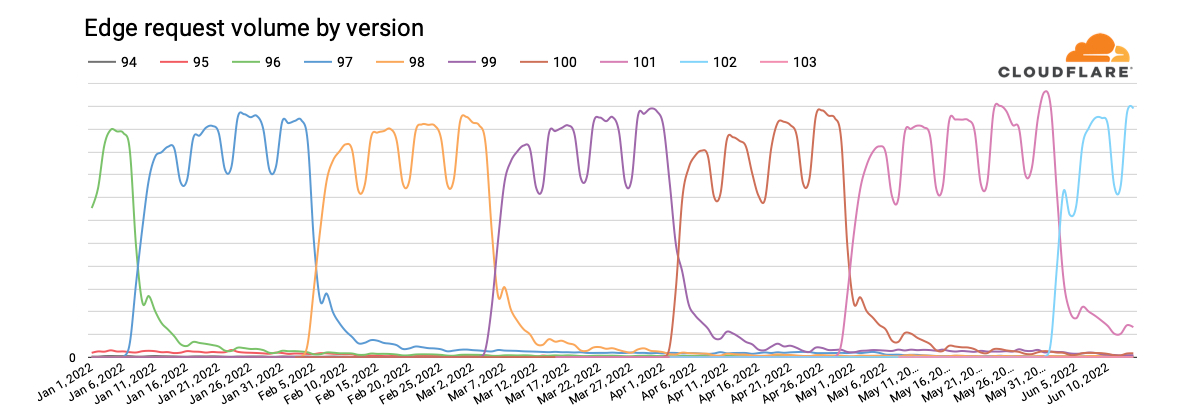
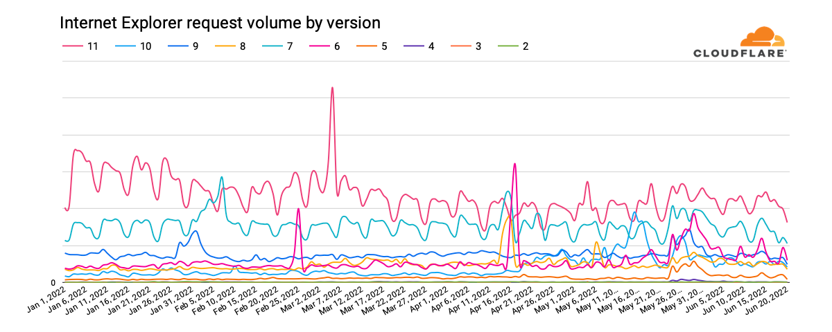
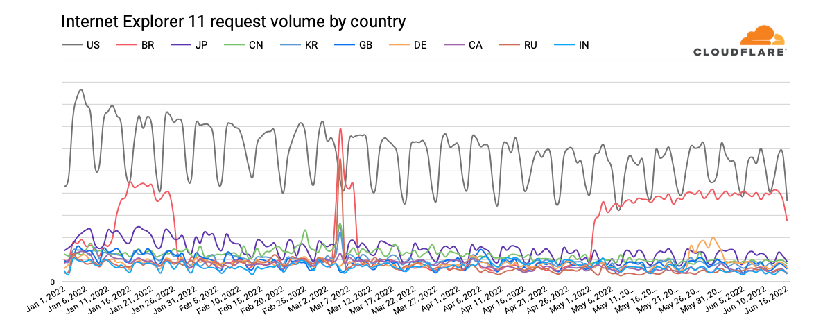
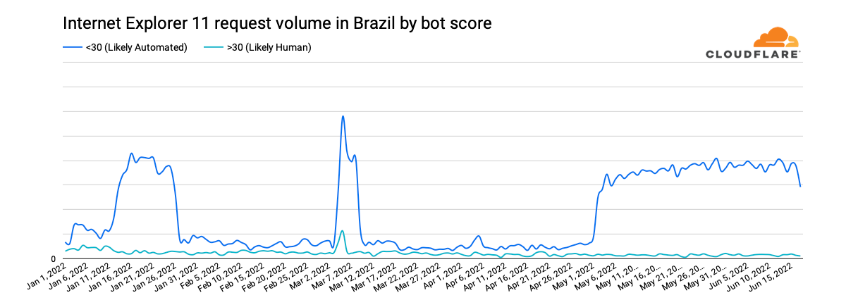
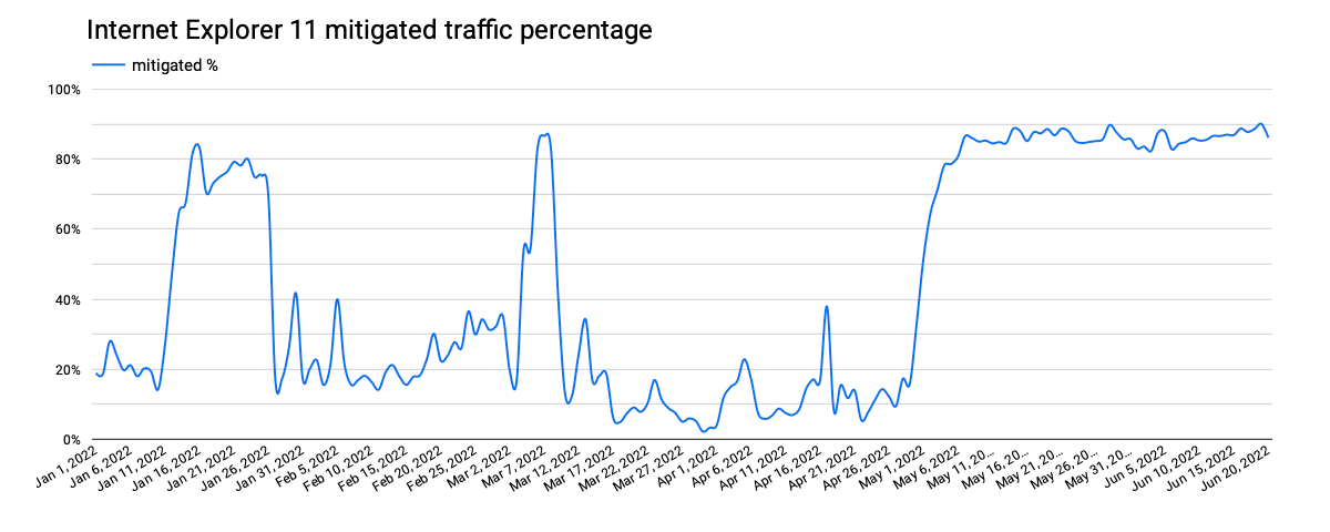
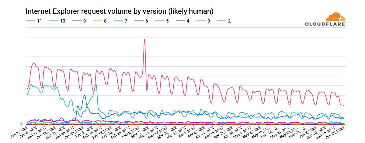
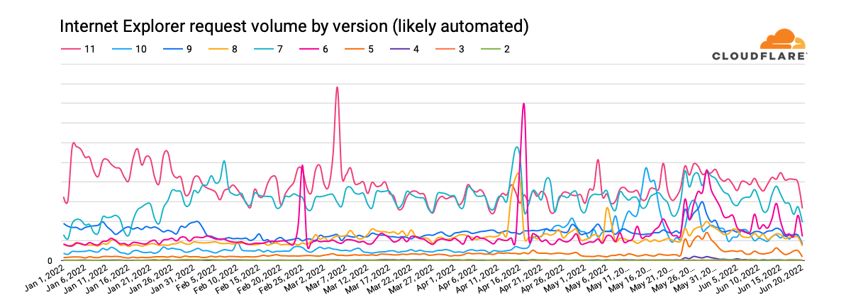
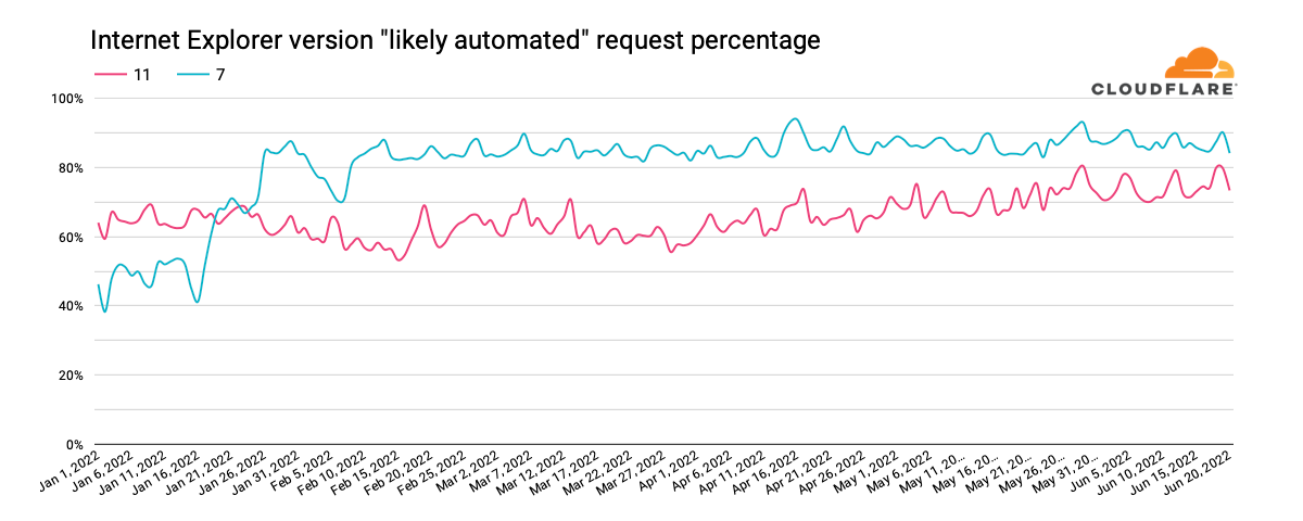
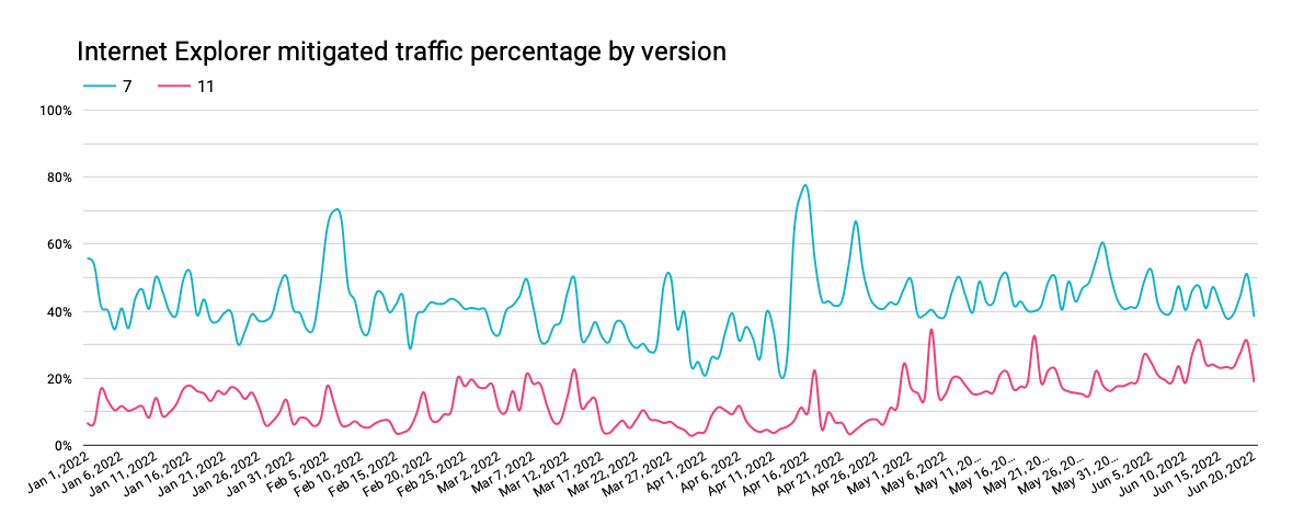
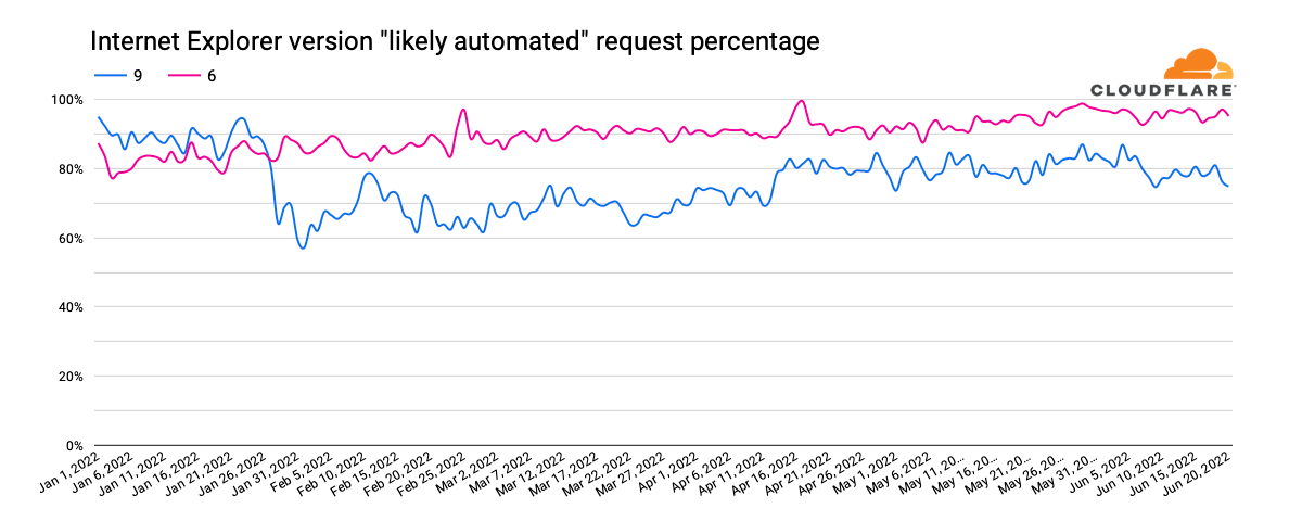
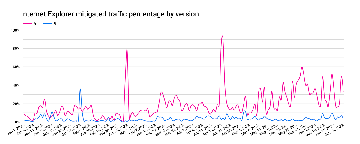


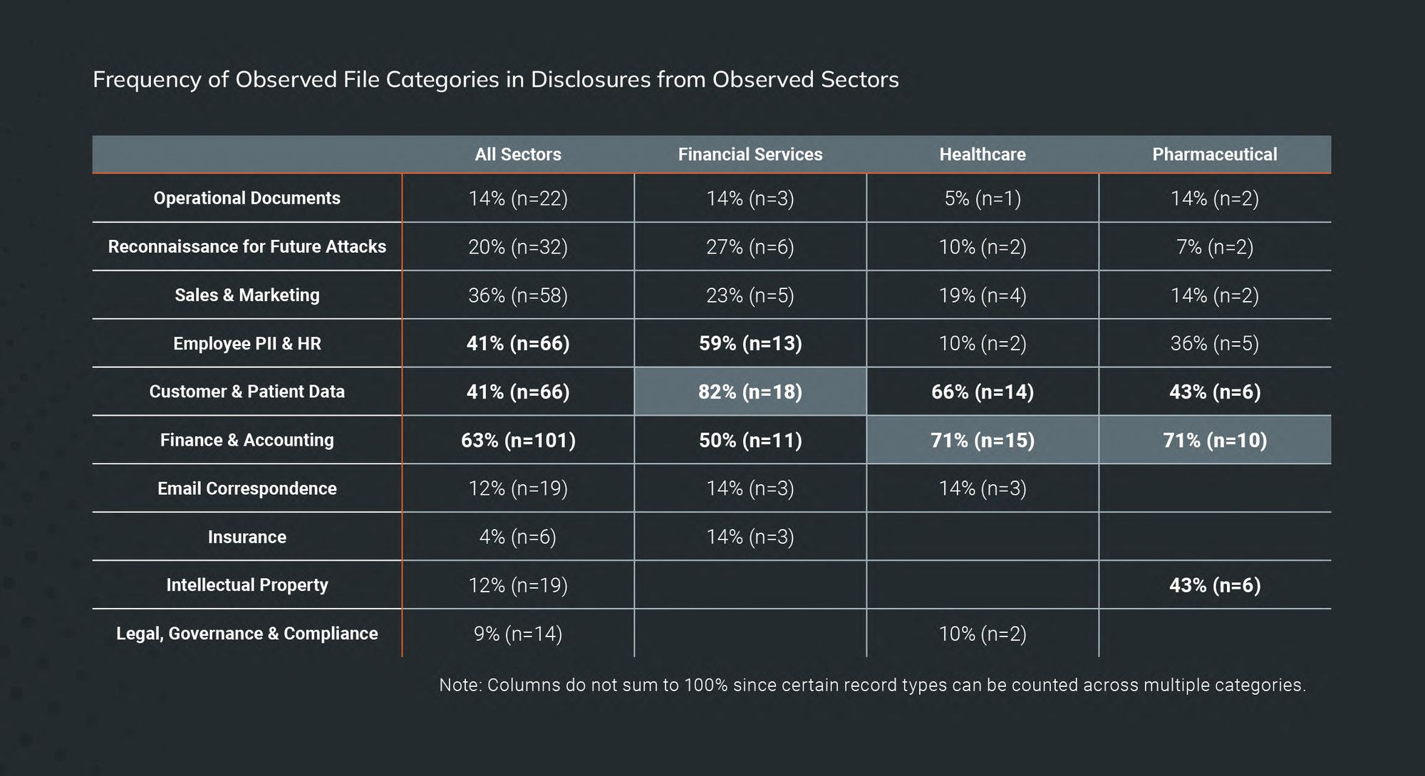


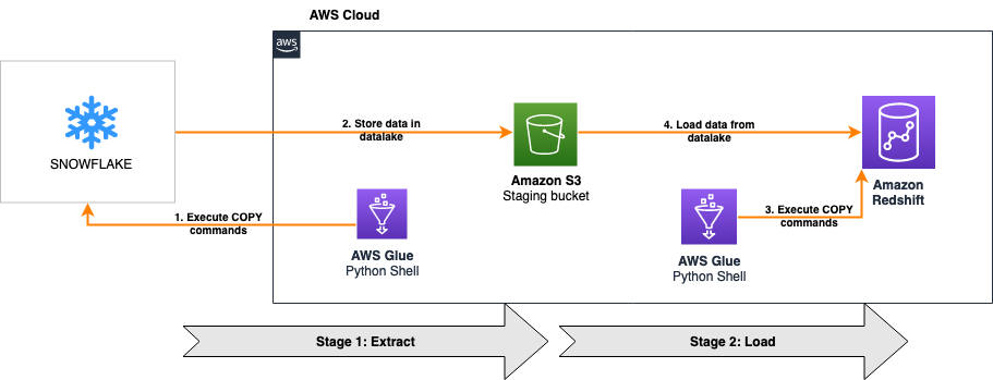


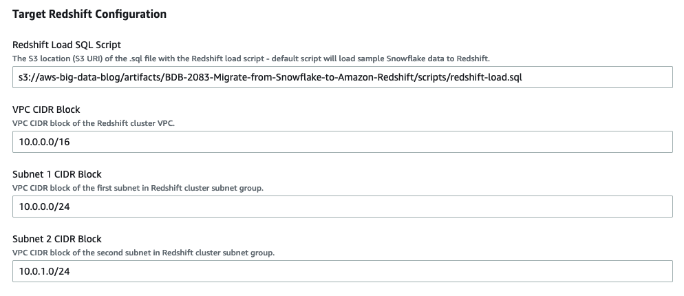

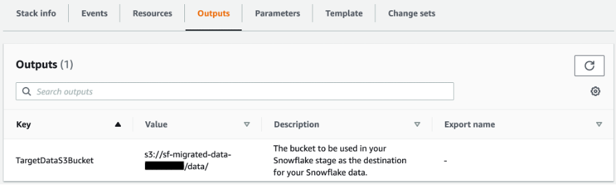

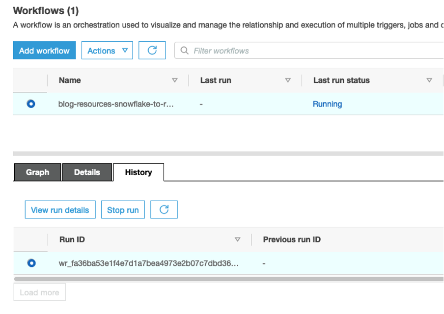


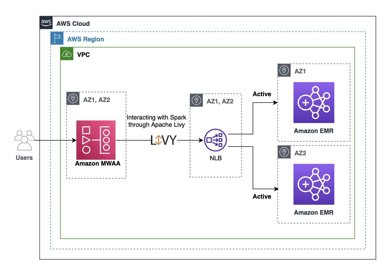
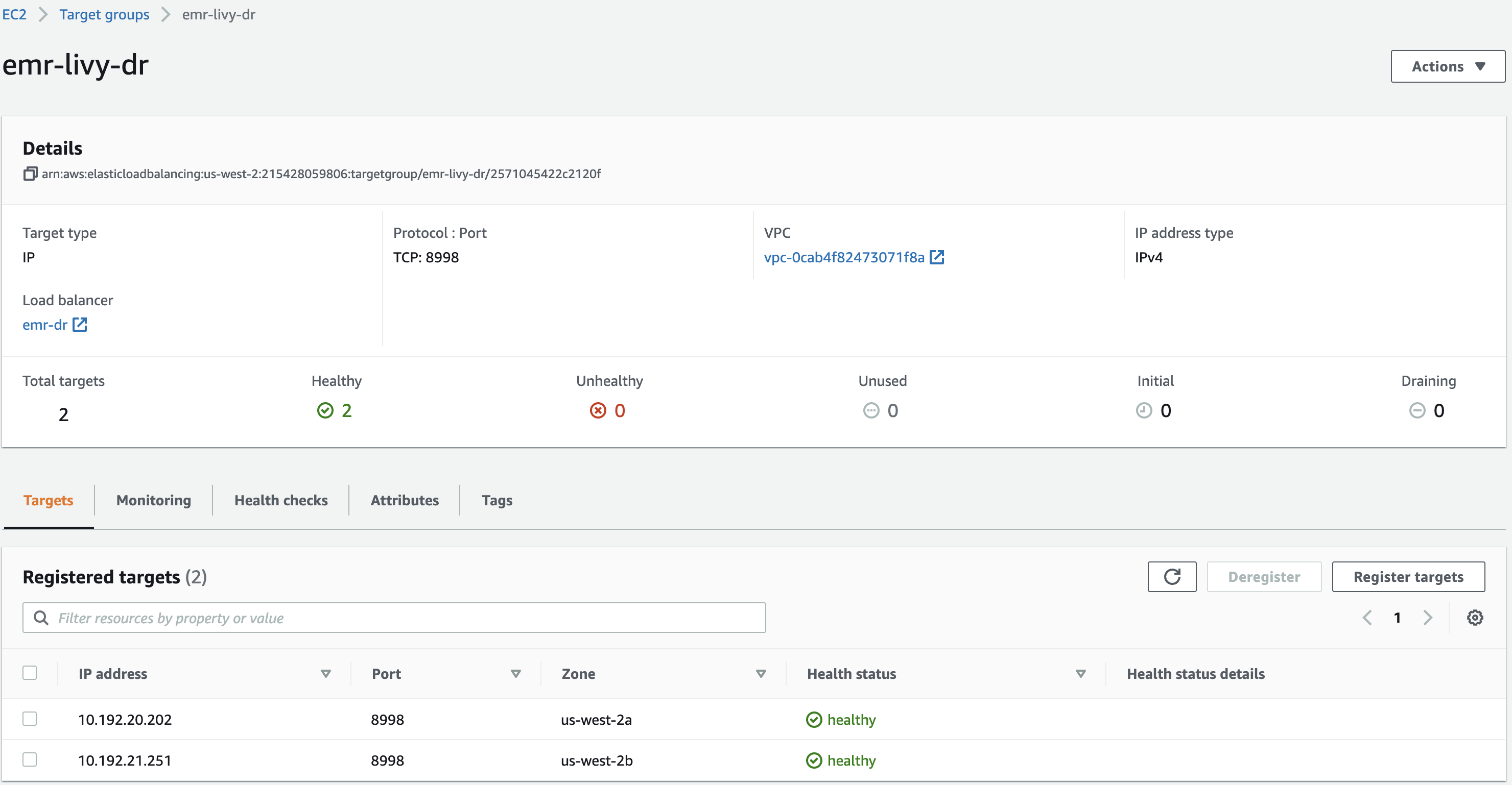
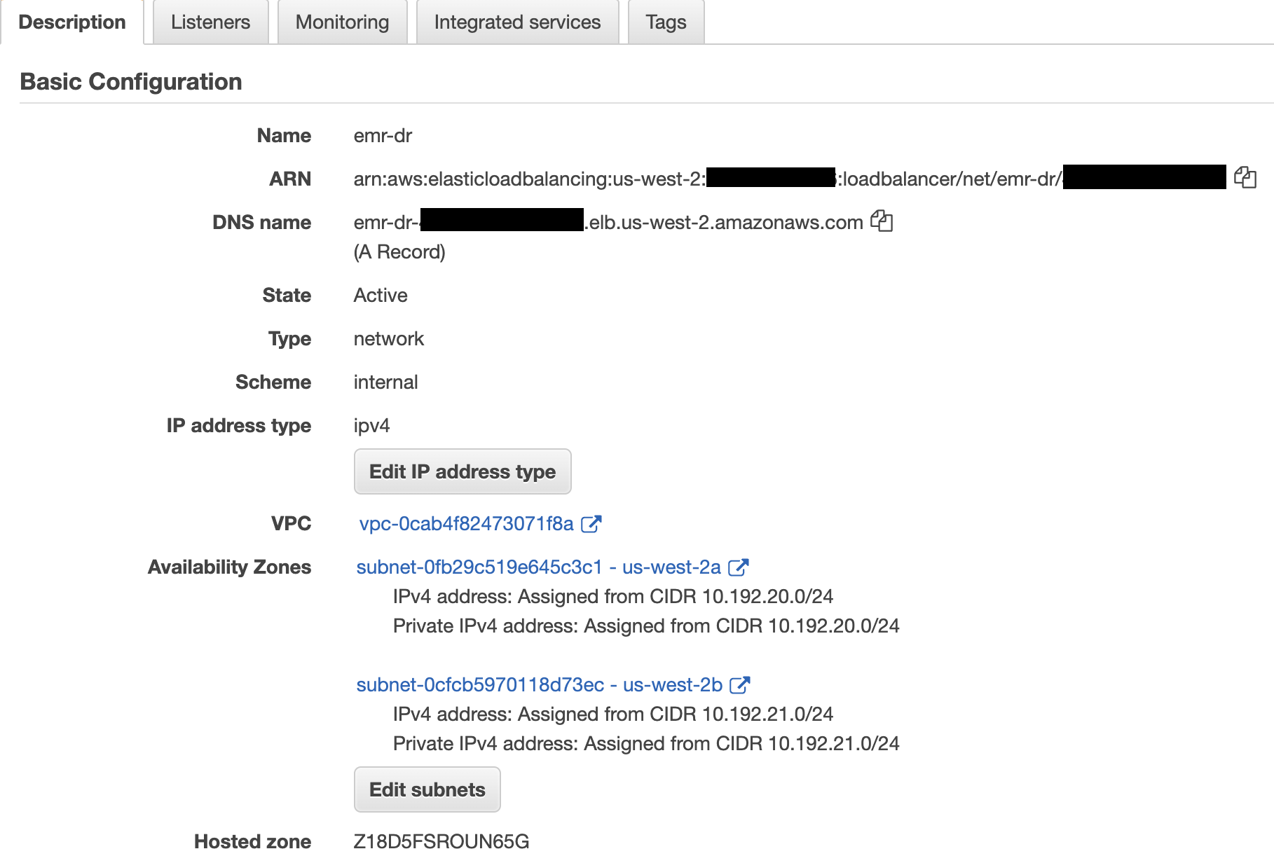

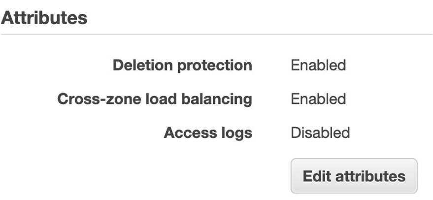
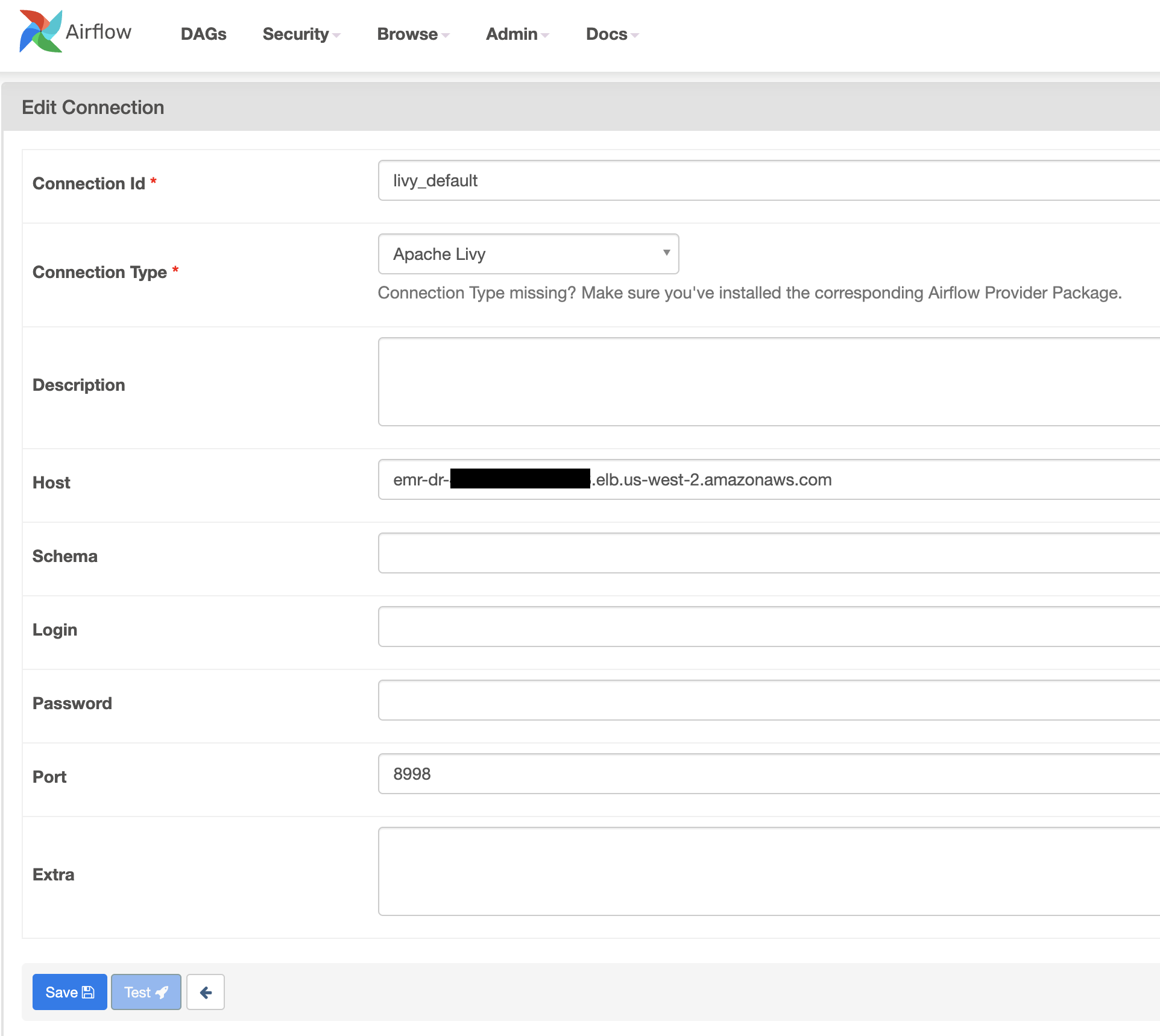

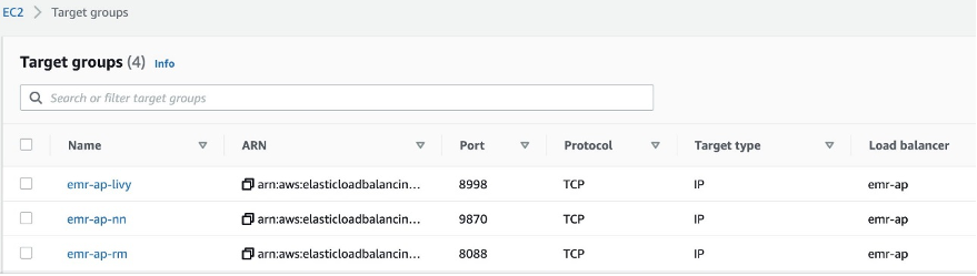
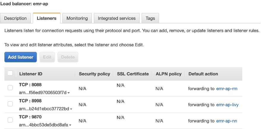
 Bharat Gamini is a Data Architect focused on Big Data & Analytics at Amazon Web Services. He helps customers architect and build highly scalable, robust and secure cloud-based analytical solutions on AWS.